Embed Size (px)
Citation preview

Final
May 2016
University Transportation Research Center - Region 2
ReportPerforming Organization: Manhattan College
Analysis of Curved WeatheringSteel Box Girder Bridges in Fire
Sponsor:University Transportation Research Center - Region 2

University Transportation Research Center - Region 2
The Region 2 University Transportation Research Center (UTRC) is one of ten original University Transportation Centers established in 1987 by the U.S. Congress. These Centers were established with the recognition that transportation plays a key role in the nation's economy and the quality of life of its citizens. University faculty members provide a critical link in resolving our national and regional transportation problems while training the professionals who address our transpor-tation systems and their customers on a daily basis.
The UTRC was established in order to support research, education and the transfer of technology in the �ield of transportation. The theme of the Center is "Planning and Managing Regional Transportation Systems in a Changing World." Presently, under the direction of Dr. Camille Kamga, the UTRC represents USDOT Region II, including New York, New Jersey, Puerto Rico and the U.S. Virgin Islands. Functioning as a consortium of twelve major Universities throughout the region, UTRC is located at the CUNY Institute for Transportation Systems at The City College of New York, the lead institution of the consortium. The Center, through its consortium, an Agency-Industry Council and its Director and Staff, supports research, education, and technology transfer under its theme. UTRC’s three main goals are:
Research
The research program objectives are (1) to develop a theme based transportation research program that is responsive to the needs of regional transportation organizations and stakehold-ers, and (2) to conduct that program in cooperation with the partners. The program includes both studies that are identi�ied with research partners of projects targeted to the theme, and targeted, short-term projects. The program develops competitive proposals, which are evaluated to insure the mostresponsive UTRC team conducts the work. The research program is responsive to the UTRC theme: “Planning and Managing Regional Transportation Systems in a Changing World.” The complex transportation system of transit and infrastructure, and the rapidly changing environ-ment impacts the nation’s largest city and metropolitan area. The New York/New Jersey Metropolitan has over 19 million people, 600,000 businesses and 9 million workers. The Region’s intermodal and multimodal systems must serve all customers and stakeholders within the region and globally.Under the current grant, the new research projects and the ongoing research projects concentrate the program efforts on the categories of Transportation Systems Performance and Information Infrastructure to provide needed services to the New Jersey Department of Transpor-tation, New York City Department of Transportation, New York Metropolitan Transportation Council , New York State Department of Transportation, and the New York State Energy and Research Development Authorityand others, all while enhancing the center’s theme.
Education and Workforce Development
The modern professional must combine the technical skills of engineering and planning with knowledge of economics, environmental science, management, �inance, and law as well as negotiation skills, psychology and sociology. And, she/he must be computer literate, wired to the web, and knowledgeable about advances in information technology. UTRC’s education and training efforts provide a multidisciplinary program of course work and experiential learning to train students and provide advanced training or retraining of practitioners to plan and manage regional transportation systems. UTRC must meet the need to educate the undergraduate and graduate student with a foundation of transportation fundamentals that allows for solving complex problems in a world much more dynamic than even a decade ago. Simultaneously, the demand for continuing education is growing – either because of professional license requirements or because the workplace demands it – and provides the opportunity to combine State of Practice education with tailored ways of delivering content.
Technology Transfer
UTRC’s Technology Transfer Program goes beyond what might be considered “traditional” technology transfer activities. Its main objectives are (1) to increase the awareness and level of information concerning transportation issues facing Region 2; (2) to improve the knowledge base and approach to problem solving of the region’s transportation workforce, from those operating the systems to those at the most senior level of managing the system; and by doing so, to improve the overall professional capability of the transportation workforce; (3) to stimulate discussion and debate concerning the integration of new technologies into our culture, our work and our transportation systems; (4) to provide the more traditional but extremely important job of disseminating research and project reports, studies, analysis and use of tools to the education, research and practicing community both nationally and internationally; and (5) to provide unbiased information and testimony to decision-makers concerning regional transportation issues consistent with the UTRC theme.
Project No(s): UTRC/RF Grant No: 49198-28-26
Project Date: May 2016
Project Title: Analysis of Curved Weathering Steel Box Girder Bridges in Fire
Project’s Website: http://www.utrc2.org/research/projects/analysis-curved-weathering-steel-box Principal Investigator(s): Dr. Reeves WhitneyVisiting InstructorManhattan CollegeRiverdale, NY 10471Tel: (718) 862-7174Email: [email protected]
Co Author(s): Nicole Leo BraxtanAssistant ProfessorManhattan [email protected]
Qian WangAssistant Professor Manhattan [email protected]
Gregory Koch
Performing Organization: Manhattan College
Sponsor(s):)University Transportation Research Center (UTRC)
To request a hard copy of our �inal reports, please send us an email at [email protected]
Mailing Address:
University Transportation Reserch CenterThe City College of New YorkMarshak Hall, Suite 910160 Convent AvenueNew York, NY 10031Tel: 212-650-8051Fax: 212-650-8374Web: www.utrc2.org

Board of Directors
The UTRC Board of Directors consists of one or two members from each Consortium school (each school receives two votes regardless of the number of representatives on the board). The Center Director is an ex-of icio member of the Board and The Center management team serves as staff to the Board.
City University of New York Dr. Hongmian Gong - Geography/Hunter College Dr. Neville A. Parker - Civil Engineering/CCNY
Clarkson University Dr. Kerop D. Janoyan - Civil Engineering
Columbia University Dr. Raimondo Betti - Civil Engineering Dr. Elliott Sclar - Urban and Regional Planning
Cornell University Dr. Huaizhu (Oliver) Gao - Civil Engineering
Hofstra University Dr. Jean-Paul Rodrigue - Global Studies and Geography
Manhattan College Dr. Anirban De - Civil & Environmental Engineering Dr. Matthew Volovski - Civil & Environmental Engineering
New Jersey Institute of Technology Dr. Steven I-Jy Chien - Civil Engineering Dr. Joyoung Lee - Civil & Environmental Engineering
New York University Dr. Mitchell L. Moss - Urban Policy and Planning Dr. Rae Zimmerman - Planning and Public Administration
Polytechnic Institute of NYU Dr. Kaan Ozbay - Civil Engineering Dr. John C. Falcocchio - Civil Engineering Dr. Elena Prassas - Civil Engineering
Rensselaer Polytechnic Institute Dr. José Holguín-Veras - Civil Engineering Dr. William "Al" Wallace - Systems Engineering
Rochester Institute of Technology Dr. James Winebrake - Science, Technology and Society/Public Policy Dr. J. Scott Hawker - Software Engineering
Rowan University Dr. Yusuf Mehta - Civil Engineering Dr. Beena Sukumaran - Civil Engineering
State University of New York Michael M. Fancher - Nanoscience Dr. Catherine T. Lawson - City & Regional Planning Dr. Adel W. Sadek - Transportation Systems Engineering Dr. Shmuel Yahalom - Economics
Stevens Institute of Technology Dr. Sophia Hassiotis - Civil Engineering Dr. Thomas H. Wakeman III - Civil Engineering
Syracuse University Dr. Riyad S. Aboutaha - Civil Engineering Dr. O. Sam Salem - Construction Engineering and Management
The College of New Jersey Dr. Thomas M. Brennan Jr - Civil Engineering
University of Puerto Rico - Mayagüez Dr. Ismael Pagán-Trinidad - Civil Engineering Dr. Didier M. Valdés-Díaz - Civil Engineering
UTRC Consortium Universities
The following universities/colleges are members of the UTRC consor-tium.
City University of New York (CUNY)Clarkson University (Clarkson)Columbia University (Columbia)Cornell University (Cornell)Hofstra University (Hofstra)Manhattan College (MC)New Jersey Institute of Technology (NJIT)New York Institute of Technology (NYIT)New York University (NYU)Rensselaer Polytechnic Institute (RPI)Rochester Institute of Technology (RIT)Rowan University (Rowan)State University of New York (SUNY)Stevens Institute of Technology (Stevens)Syracuse University (SU)The College of New Jersey (TCNJ)University of Puerto Rico - Mayagüez (UPRM)
UTRC Key Staff
Dr. Camille Kamga: Director, Assistant Professor of Civil Engineering
Dr. Robert E. Paaswell: Director Emeritus of UTRC and Distinguished Professor of Civil Engineering, The City College of New York
Herbert Levinson: UTRC Icon Mentor, Transportation Consultant and Professor Emeritus of Transportation
Dr. Ellen Thorson: Senior Research Fellow, University Transportation Research Center
Penny Eickemeyer: Associate Director for Research, UTRC
Dr. Alison Conway: Associate Director for Education
Nadia Aslam: Assistant Director for Technology Transfer
Nathalie Martinez: Research Associate/Budget Analyst
Tierra Fisher: Of ice Assistant
Bahman Moghimi: Research Assistant; Ph.D. Student, Transportation Program
Wei Hao: Research Fellow
Andriy Blagay: Graphic Intern
Membership as of January 2016

TECHNICAL REPORT STANDARD TITLE PAGE
1. Report No. 2.Government Accession No. 3. Recipient’s Catalog No.
4. Title and Subtitle 5. Report Date 5/31/2016 Analysis of Curved Weathering Steel Box Girder Bridges in Fire
6. Performing Organization Code
7. Author(s) 8. Performing Organization Report No. Reeves Whitney, Nicole Leo Braxtan, Qian Wang, Gregory Koch
9. Performing Organization Name and Address 10. Work Unit No. Department of Civil and Environmental Engineering Manhattan College 4513 Manhattan College Parkway Bronx, NY 10471
11. Contract or Grant No.
49198-28-26
12. Sponsoring Agency Name and Address 13. Type of Report and Period Covered University Transportation Research Center Marshak Hall – Science Building, Suite 910 The City College of New York 138th Street & Convent Avenue, New York, NY 10031
14. Sponsoring Agency Code
15. Supplementary Notes
16. Abstract Box girder bridges are becoming more common because of their ease of construction, pleasing aesthetics, and serviceability. Projects with curved configuration and long spans can especially benefit from these advantages. However, the industry lacks a wide range of research on multi-span steel box girder cross-sections and their response to fire events. In addition, steel box girders are commonly constructed from weathering steel, which has little available research into their performance in fire. This paper will discuss the current literature, challenges, and available verification studies for this particular combination of cross section and material properties. Results show large deflections in the steel box girder as the temperature of the steel increases over the duration of the fire. Temperatures of the steel tub increase rapidly due to the low weight-to-heated perimeter ratio of the thin members. The concrete slab does not exhibit significant increase in temperature from the fire below. Furthermore, forces that act on the individual members of the bridge are greatly affected by the location of the fire.
17. Key Words 18. Distribution Statement Steel box girder, composite bridges, fire, thermal analysis, finite element
19. Security Classif (of this report) 20. Security Classif. (of this page) 21. No of Pages 22. Price
Unclassified Unclassified
Form DOT F 1700.7 (8-69)

i
Disclaimer
The contents of this report reflect the views of the authors, who are responsible for the facts and the accuracy of the information presented herein. The contents do not necessarily reflect the official views or policies of the UTRC, or the Federal Highway Administration. This report does not constitute a standard, specification or regulation. This document is disseminated under the sponsorship of the Department of Transportation, University Transportation Centers Program, in the interest of information exchange. The U.S. Government assume no liability for the contents or use thereof.

ii
Contents 1 Introduction ............................................................................................................................. 1
1.1 Goals and Objectives ........................................................................................................ 1
2 Background research activites/framework .............................................................................. 2
2.1 Literature Review ............................................................................................................. 2
2.2 Fire Properties .................................................................................................................. 3
2.2.1 Hydrocarbon Fire ...................................................................................................... 3
2.2.2 Heat Transfer ............................................................................................................ 4
2.2.3 Distance Dependent Fire Intensity ............................................................................ 6
2.3 Steel Properties ................................................................................................................. 6
2.3.1 Steel Thermal Properties ........................................................................................... 6
2.3.2 Steel Structural Properties......................................................................................... 7
2.4 Concrete Properties .......................................................................................................... 9
2.4.1 Concrete Thermal Properties .................................................................................... 9
2.4.2 Concrete Structural Properties ................................................................................ 10
2.4.3 Cast Iron Model Applied to Reinforced Concrete .................................................. 11
2.5 Finite Element Modeling ................................................................................................ 12
2.5.1 Hardware/Software ................................................................................................. 12
2.5.2 Elements .................................................................................................................. 12
2.6 Model validation ............................................................................................................ 14
2.6.1 Case Study .............................................................................................................. 14
2.6.2 Model Parameters ................................................................................................... 15
3 Straight Box Girder ............................................................................................................... 20
3.1 Geometry ........................................................................................................................ 20
3.1.1 Cross Section .......................................................................................................... 20
3.1.2 Elevation ................................................................................................................. 21
3.1.3 Internal Bracing ...................................................................................................... 21
3.2 Finite Element Model ..................................................................................................... 22
3.3 Fire Scenarios and Thermal Boundary Conditions ........................................................ 22
3.4 Structural Boundary Conditions ..................................................................................... 25
3.5 AASHTO Design Requirements .................................................................................... 25
3.5.1 Shear Resistance ..................................................................................................... 25
3.5.2 Moment Capacity .................................................................................................... 27
3.6 Heat Transfer Results ..................................................................................................... 28

iii
3.7 Structural Results ........................................................................................................... 29
3.8 End Restraint Investigation ............................................................................................ 35
4 Curved Box Girder ................................................................................................................ 37
4.1 Geometry ........................................................................................................................ 37
4.1.1 Cross Section .......................................................................................................... 37
4.1.2 Elevation ................................................................................................................. 38
4.1.3 Framing ................................................................................................................... 39
4.2 Finite Element Model ..................................................................................................... 39
4.3 Fire Scenario and Location ............................................................................................ 39
4.4 Support Conditions ......................................................................................................... 41
4.5 Heat Transfer Results ..................................................................................................... 41
4.6 Structural Results ........................................................................................................... 43
4.7 End Restraint Investigation ............................................................................................ 47
5 Conclusion ............................................................................................................................ 50
6 Future Works ........................................................................................................................ 50
7 Acknowledgements ............................................................................................................... 51
References ..................................................................................................................................... 51

iv
Table of Figures
Figure 1 - Temperature of fire with respect to time ........................................................................ 4
Figure 2 - Thermal loading fire properties: reduction factor with respect to distance. .................. 6 Figure 3 -Temperature dependent thermal properties of weathering steel and traditional steel: (a)
conductivity; (b) specific heat; and (c) thermal expansion. ........................................... 7 Figure 4 - Temperature dependent stress-strain curves for weathering steel. ................................. 8 Figure 5 - Temperature dependent stress-strain curves for traditional steel. .................................. 8
Figure 6 - Temperature dependent material properties of weathering steel and traditional steel:
(a) yield strength; (b) Young’s Modulus ........................................................................ 9 Figure 7 - Temperature dependent thermal properties of siliceous and calcareous concrete: (a)
conductivity; (b) specific heat. ....................................................................................... 9 Figure 8 - Temperature dependent stress-strain curves of siliceous concrete. ............................. 10
Figure 9 - Temperature dependent stress-strain curves of calcareous concrete. ........................... 10 Figure 10 - Temperature dependent compressive strength of siliceous and calcareous concrete 11
Figure 11 - Cast iron stress-strain relationship model applied to concrete ................................... 11 Figure 12 - Basic Element Types .................................................................................................. 12
Figure 13 – Conventional versus continuum shell models ........................................................... 13 Figure 14 - Cross section of composite beam ............................................................................... 15 Figure 15 - Elevation view of beam showing fire application area, supports, and loading points 15
Figure 16 - Cross section of beam showing thermal boundary conditions ................................... 16 Figure 17 - Cross section of beam and slab showing locations used for temperature analysis17
Figure 18 - Comparison of Abaqus data and laboratory test for temperature data. ...................... 18 Figure 19 - Comparison of Abaqus data and laboratory test.. ...................................................... 19 Figure 20 - Cross section of straight box girder bridge Abaqus model. ....................................... 20
Figure 21 - Full straight box girder bridge model......................................................................... 20
Figure 22 - Cross sectional dimensions of the straight steel box girder bridge ............................ 21 Figure 23 - Elevation view of the straight box girder bridge showing plate thickness. ............... 21 Figure 24 - Framing plan of the straight bridge showing view of all bracing members............... 22
Figure 25 - Midspan fire location of the straight bridge with fire reduction curve ...................... 23 Figure 26 - Pier fire location of the straight bridge with fire reduction curve .............................. 23 Figure 27 - Convection and emissivity values used in the thermal model ................................... 24
Figure 28- Support conditions of the straight box girder bridge .................................................. 25 Figure 29 – Plastic analysis with stress block in the flange .......................................................... 27 Figure 30 - Cross section of the straight box girder bridge showing node locations.................... 29 Figure 31 - Comparison of element temperatures versus time of the straight bridge. .................. 29 Figure 32 - Temperature of the line element directly over the full strength fire .......................... 30
Figure 33 - Comparison of maximum bridge deflection of the straight box girder bridge. ......... 30 Figure 34 - Deflected shape and Mises stress of the straight box girder bridge corresponding to
fire location 1. ............................................................................................................... 32 Figure 35 - Deflected shape and Mises stress of the straight box girder bridge corresponding to
fire location 2. ............................................................................................................... 32 Figure 36 – Final step of analysis corresponding to fire location 2. ............................................. 33 Figure 37 - Final step of analysis corresponding to fire location 1. ............................................. 33 Figure 38 - Maximum deflection at point D2 compared to the shear demand/capacity ratio. ..... 34 Figure 39 - Maximum deflection at point D1 compared to the moment demand/capacity ratio. . 34

v
Figure 40 - Support conditions of the straight box girder bridge with additional end restraint. .. 35
Figure 41 - Vertical deflection of the straight steel box girder bridge. ......................................... 36 Figure 42 – Cross sectional dimensions of the curved steel box girder bridge ............................ 37 Figure 43 – Cross section of curved box girder bridge Abaqus model. ....................................... 37
Figure 44 –Full curved box girder bridge model. ......................................................................... 38 Figure 45 - Elevation view of the curved box girder bridge ......................................................... 38 Figure 46 - Plan view of the curved box girder bridge showing framing. .................................... 39 Figure 47 - Midspan fire location of curved bridge with fire reduction curve. ............................ 40 Figure 48 - Pier fire location of curved bridge with fire reduction curve. .................................... 40
Figure 49 - Support conditions of the curved box girder bridge................................................... 41 Figure 50 - Cross section of the curved box girder bridge showing node locations. ................... 42 Figure 51 - Element temperatures verses time of the curved box girder bridge ........................... 42 Figure 52 - Comparison of maximum deflection of the curved box girder bridge. ...................... 44
Figure 53 - Deflected shape and Mises stress of the curved box girder bridge corresponding to
fire location 2. ............................................................................................................... 45
Figure 54 - Deflected shape and Mises stress of the curved box girder bridge corresponding to
fire location 1. ............................................................................................................... 45
Figure 55 - Final step of analysis corresponding to fire location 2. ............................................. 46 Figure 56 - Final step of analysis corresponding to fire location 1. ............................................. 46 Figure 57 - Maximum deflection at point D2 compared to the shear demand/capacity ratio ...... 46
Figure 58 - Maximum deflection at point D1 compared to the moment demand/capacity ratio .. 47 Figure 59 - Adjusted support conditions of the curved box girder bridge with addition end
restraint. ........................................................................................................................ 48 Figure 60 - Vertical deflection of the curved box girder bridge with two different support
conditions. .................................................................................................................... 48
Figure 61 - Horizontal deflection of the curved box girder bridge ............................................... 49

1
1 INTRODUCTION
Bridge fires can present a severe hazard to the transportation infrastructure system. In fact,
a nationwide survey by the New York State Department of Transportation (NYSDOT) has shown
that fires have collapsed approximately three times as many bridges as earthquakes (Garlock et al.
2013). Bridge fires are often intense as they may be fueled by gasoline from vehicles that have
crashed in the vicinity of the bridge. Additionally, code recommendations and guidelines for fire
protection of bridges are lax. Large fuel loads and a lack of code requirements for fire protection
of bridges have left bridges quite vulnerable to fire, particularly unprotected steel bridges, which
was established in recent research (Labbouz 2014). The research focus has mainly been on
traditional carbon steels at elevated temperatures and bridges of simple geometry such as plate
girders. It is therefore necessary to expand on this research to include additional materials such as
weathering steel and additional bridge geometries such as curved box girders.
Weathering steel has been widely used by State DOTs for construction of steel bridges
because of the maintenance cost savings. New York State DOT’s preferred structural steel for
bridge girders is weathering steel, and it was reported that they owned more than 1200 weathering
steel bridges in 2000 (Labbouz 2014). Weathering steel forms a protective layer of rust (patina)
to prevent corrosion of the steel and only recently have the mechanical properties of weathering
steel at elevated temperatures been determined (Cor-Ten 2014, Labbouz 2014). The determination
of these properties allows for discussion of the behavior of weathering steels in fire.
1.1 Goals and Objectives
The goal of this work is to determine critical parameters for curved steel box girders
exposed to fire. This goal will be evaluated through a series of objectives which consider both
thermal and structural consequences for weathering steel box girders subject to fire loading.
The objectives of the proposed work include: (1) determine critical location for fire in steel
box girders; (2) determine critical temperature history and fire intensity for steel box girders; and
(3) determine the reduction in bending moment and shear capacity – and thus load-carrying
capacity – of steel box girders exposed to fire.
To complete these objectives, this research was conducted using three major tasks in order
to build knowledge of the task at hand. Task one consisted of finite element modeling and
validation of fire effects on steel structures. This was carried out by comparing published
laboratory test results (Wainman et al. 1987) with a computer model of a steel beam with a concrete
slab. The second task involved the modeling and analysis of a straight box girder bridge. This
leads into the third task which entailed the study of a curved box girder. Each of these steps will
be explained in detail along with the resulting data from each task.
2
2 BACKGROUND RESEARCH ACTIVITES/FRAMEWORK
2.1 Literature Review
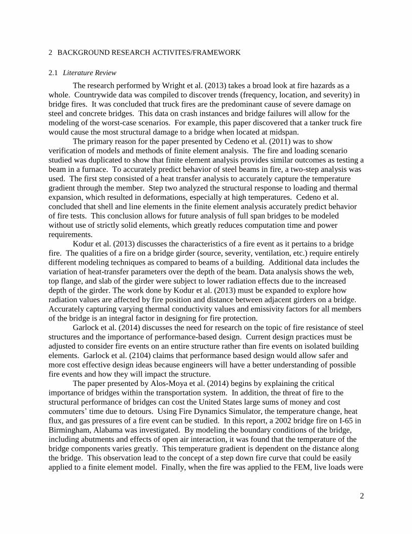
The research performed by Wright et al. (2013) takes a broad look at fire hazards as a
whole. Countrywide data was compiled to discover trends (frequency, location, and severity) in
bridge fires. It was concluded that truck fires are the predominant cause of severe damage on
steel and concrete bridges. This data on crash instances and bridge failures will allow for the
modeling of the worst-case scenarios. For example, this paper discovered that a tanker truck fire
would cause the most structural damage to a bridge when located at midspan.
The primary reason for the paper presented by Cedeno et al. (2011) was to show
verification of models and methods of finite element analysis. The fire and loading scenario
studied was duplicated to show that finite element analysis provides similar outcomes as testing a
beam in a furnace. To accurately predict behavior of steel beams in fire, a two-step analysis was
used. The first step consisted of a heat transfer analysis to accurately capture the temperature
gradient through the member. Step two analyzed the structural response to loading and thermal
expansion, which resulted in deformations, especially at high temperatures. Cedeno et al.
concluded that shell and line elements in the finite element analysis accurately predict behavior
of fire tests. This conclusion allows for future analysis of full span bridges to be modeled
without use of strictly solid elements, which greatly reduces computation time and power
requirements.
Kodur et al. (2013) discusses the characteristics of a fire event as it pertains to a bridge
fire. The qualities of a fire on a bridge girder (source, severity, ventilation, etc.) require entirely
different modeling techniques as compared to beams of a building. Additional data includes the
variation of heat-transfer parameters over the depth of the beam. Data analysis shows the web,
top flange, and slab of the girder were subject to lower radiation effects due to the increased
depth of the girder. The work done by Kodur et al. (2013) must be expanded to explore how
radiation values are affected by fire position and distance between adjacent girders on a bridge.
Accurately capturing varying thermal conductivity values and emissivity factors for all members
of the bridge is an integral factor in designing for fire protection.
Garlock et al. (2014) discusses the need for research on the topic of fire resistance of steel
structures and the importance of performance-based design. Current design practices must be
adjusted to consider fire events on an entire structure rather than fire events on isolated building
elements. Garlock et al. (2104) claims that performance based design would allow safer and
more cost effective design ideas because engineers will have a better understanding of possible
fire events and how they will impact the structure.
The paper presented by Alos-Moya et al. (2014) begins by explaining the critical
importance of bridges within the transportation system. In addition, the threat of fire to the
structural performance of bridges can cost the United States large sums of money and cost
commuters’ time due to detours. Using Fire Dynamics Simulator, the temperature change, heat
flux, and gas pressures of a fire event can be studied. In this report, a 2002 bridge fire on I-65 in
Birmingham, Alabama was investigated. By modeling the boundary conditions of the bridge,
including abutments and effects of open air interaction, it was found that the temperature of the
bridge components varies greatly. This temperature gradient is dependent on the distance along
the bridge. This observation lead to the concept of a step down fire curve that could be easily
applied to a finite element model. Finally, when the fire was applied to the FEM, live loads were
3
applied along the bridge span. It was found that live load has a very small effect on the response
of the bridge during a fire event.
The research performed by Xu (2015) investigates the effects of fire on orthotropic steel
deck bridges. In addition, the effect on cable supported bridges are modeled. One main topic is
the effect of the vertical distance that the fire occurs below the bridge. Also, fires that occur on
top of the bridge are investigated. Additional parameters include power of fire, steel strength,
and axial load applied to the bridge members. Finally, a case study is performed to analyze the
fire that occurred in 2013 under the Ed Koch Queensboro Bridge.
Labboz (2014) investigates the strength and other properties of weathering steel at
elevated temperatures. Weathering steel elements are exposed to high temperatures and tested to
determine the effect of fire on this material. Using multiple samples, temperatures, and cooling
methods, a full range of strength reduction factors are found for increasing temperatures. These
results are used in a Finite Element Model. A case study is then performed on an I-195 bridge
fire to further investigate the materials used in this bridge.
In the research done by Baskar et al. (2002), steel-concrete composite girders were
analyzed using finite element modeling. One very important part of this modeling was the analysis
of the tensile behavior of the concrete slab that rests on top of the steel beam. This becomes a
difficult task in models in which many cracks occur because cracks effect the calculations using a
damaged elasticity model. Baskar et al. modeled the concrete using three material models. The
first was using the concrete model in which the concrete will crack at a certain ultimate tensile
stress. After this point, the concrete softens linearly to the point in which it can no longer hold any
load. The second model uses the Cast Iron model. Using this model, once the ultimate tensile
stress is reached, the stress strain plot flattens out resulting in a constant stress as strain increases.
The final material model used is the Elastic-Plastic model. Using this definition, concrete is
assumed to behave the same in both tension and compression. The authors draw the conclusion
that using the Cast Iron model allows the FEM to predict an ultimate load that is closer the
experimental value.
2.2 Fire Properties
2.2.1 Hydrocarbon Fire
Fires vary in intensity based on given fuel sources and ventilation factors. Additionally,
effects of the fire on a structure will vary based on geometry of the structure and proximity to the
fire. The research described in this report assumed that a hydrocarbon fueled fire occurred
directly below the bridge.
Eurocode I (CEN 2002) documents three possible fire scenarios: standard temperature-
time, external fire, and hydrocarbon curves. To simulate a worst case scenario, the hydrocarbon
fire was chosen to represent an event in which a tanker truck carrying gasoline ignited under a
bridge. The hydrocarbon fire curve equation is shown in Eq. (1).
Ѳ𝑔 = 1080 ∗ (1 − 0.325𝑒−0.167𝑡 − 0.675𝑒−2.5𝑡) + 20 ( 1)
𝑤ℎ𝑒𝑟𝑒: Ѳ𝑔 = 𝑔𝑎𝑠 𝑡𝑒𝑚𝑝𝑒𝑟𝑎𝑡𝑢𝑟𝑒 𝑖𝑛 𝑡ℎ𝑒 𝑓𝑖𝑟𝑒 𝑐𝑜𝑚𝑝𝑎𝑟𝑡𝑚𝑒𝑛𝑡
𝑡 = 𝑡𝑖𝑚𝑒

4
Equation 1 shows that the gas temperature will range from 20 °C to 1100 °C. Figure 1 shows the
gas temperature versus time. It can be seen that at 20 minutes, the temperature is approximately
at the maximum of 1100 °C.
Figure 1- Temperature of fire with respect to time
2.2.2 Heat Transfer
Heat is transferred from the fire (gas temperature) to the bridge elements through the three
basic mechanisms of heat transfer: convection, conduction, and radiation. The basic governing
equations for the three mechanisms are discussed in the following sections. Additional theory
can be found by referring to various texts on the subject, such as Bergman et al. (2011).
2.2.2.1 Conduction
Conduction is the transfer of heat through a solid. This will occur within the bridge itself
when heat is transferred between adjacent points of the bridge. Conduction can be described by
Fourier’s Law shown in Eq. (2) (Bergman et al. 2011).
𝑞𝑐𝑜𝑛𝑑 = −𝑘𝑑𝑇
𝑑𝑥 ( 2)
𝑤ℎ𝑒𝑟𝑒:
𝑞𝑐𝑜𝑛𝑑 = 𝑐𝑜𝑛𝑑𝑢𝑐𝑡𝑖𝑜𝑛 ℎ𝑒𝑎𝑡 𝑓𝑙𝑢𝑥,𝑊
𝑚2
𝑘 = 𝑡ℎ𝑒𝑟𝑚𝑎𝑙 𝑐𝑜𝑛𝑑𝑢𝑐𝑡𝑖𝑣𝑖𝑡𝑦,𝑤
𝑚 ∗ 𝐾
𝑑𝑇
𝑑𝑥= 𝑡𝑒𝑚𝑝𝑒𝑟𝑎𝑡𝑢𝑟𝑒 𝑔𝑟𝑎𝑑𝑖𝑒𝑛𝑡
0
200
400
600
800
1000
1200
0 20 40 60
Tem
per
atu
re, °C
Time, min

5
As Eq. (2) shows, a higher thermal conductivity will result in a faster rate of heat transfer. The
thermal conductivity of a material is temperature dependent and will be defined for each material
in sections 2.3.1 and 2.4.1 of this paper.
2.2.2.2 Convection
Convection is the transfer of heat between moving fluids, in this case air at elevated fire
temperatures, to a solid surface (the bridge); natural convection causes hot gases to rise.
Convection is described by Newton’s Law of Cooling in Eq. (3) (Bergman et al. 2011).
𝑞𝑐𝑜𝑛𝑣 = ℎ(𝑇𝑓 − 𝑇𝑠) ( 3)
𝑤ℎ𝑒𝑟𝑒:
𝑞𝑐𝑜𝑛𝑣 = 𝑐𝑜𝑛𝑣𝑒𝑐𝑡𝑖𝑜𝑛 ℎ𝑒𝑎𝑡 𝑓𝑙𝑢𝑥,𝑊
𝑚2
ℎ = 𝑐𝑜𝑛𝑣𝑒𝑐𝑡𝑖𝑜𝑛 𝑐𝑜𝑒𝑓𝑓𝑖𝑐𝑖𝑒𝑛𝑡,𝑤
𝑚 ∗ 𝐾
𝑇𝑓 = 𝑡𝑒𝑚𝑝𝑒𝑟𝑎𝑡𝑢𝑟𝑒 𝑜𝑓 𝑡ℎ𝑒 𝑓𝑙𝑢𝑖𝑑, 𝐾
𝑇𝑠 = 𝑡𝑒𝑚𝑝𝑒𝑟𝑎𝑡𝑢𝑟𝑒 𝑜𝑓 𝑡ℎ𝑒 𝑠𝑢𝑟𝑓𝑎𝑐𝑒, 𝐾
It can be seen in Eq. (3) that temperature large temperature difference between the air and the
surface causes a greater heat flux due to convection.
2.2.2.3 Radiation
Radiation heat transfer is defined as the energy transfer of electromagnetic waves
between two bodies. In the case of a fire, the fire itself is considered a body and the structure is
the second body. The effects of radiation are shown in Eq. (4) (Bergman et al. 2011).
𝑞𝑟𝑎𝑑 = 𝜀𝑠𝜀𝑡𝜎(𝑇𝑠4 − 𝑇𝑢
4) ( 4) 𝑤ℎ𝑒𝑟𝑒:
𝑞𝑟𝑎𝑑 = 𝑟𝑎𝑑𝑖𝑎𝑡𝑖𝑜𝑛 ℎ𝑒𝑎𝑡 𝑓𝑙𝑢𝑥,𝑊
𝑚2
𝜀𝑠 = 𝑒𝑚𝑖𝑠𝑠𝑖𝑣𝑖𝑡𝑦 𝑜𝑓 𝑡ℎ𝑒 𝑠𝑢𝑟𝑓𝑎𝑐𝑒 𝜀𝑡 = 𝑒𝑚𝑖𝑠𝑠𝑖𝑣𝑖𝑡𝑦 𝑜𝑓 𝑡ℎ𝑒 𝑓𝑖𝑟𝑒
𝜎 = 𝑆𝑡𝑒𝑓𝑎𝑛 − 𝐵𝑜𝑙𝑡𝑧𝑚𝑎𝑛 𝑐𝑜𝑛𝑠𝑡𝑛𝑎𝑡, 5.67𝑒 − 08𝑊
𝑚2 ∗ 𝐾4
𝑇𝑠 = 𝑡𝑒𝑚𝑝𝑒𝑟𝑎𝑡𝑢𝑟𝑒 𝑜𝑓 𝑡ℎ𝑒 𝑠𝑢𝑟𝑓𝑎𝑐𝑒, 𝐾 𝑇𝑢 = 𝑡𝑒𝑚𝑝𝑒𝑟𝑎𝑡𝑢𝑟𝑒 𝑜𝑓 𝑡ℎ𝑒 𝑠𝑢𝑟𝑟𝑜𝑢𝑛𝑑𝑖𝑛𝑔𝑛𝑛𝑠, 𝐾
6
Radiative heat transfer is highly nonlinear as it is based on temperature to the fourth power. This
causes large changes in temperature of the surface when there is a large temperature difference
between the surface and surroundings.
The total heat flux on a system is found by adding Eq. (2), (3), and (4) as shown in the
total heat flux equation, Eq. (5).
𝑞𝑡𝑜𝑡𝑎𝑙 = 𝑞𝑐𝑜𝑛𝑑 + 𝑞𝑐𝑜𝑛𝑣 + 𝑞𝑟𝑎𝑑 ( 5)
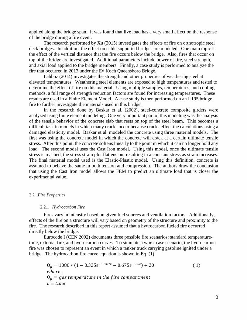
2.2.3 Distance Dependent Fire Intensity
Due to the long span of the bridge, a model was created to represent the relationship
between fire intensity and longitudinal distance from the fire. A fire gradient created by Alos-
Moya et al. (2014) was adapted for application to a steel box girder. The hydrocarbon fire was
sectioned into five meter segments that decreased in temperature as the longitudinal distance
from the center of fire increased. Figure 2 shows the time dependent hydrocarbon fire curve
along with the distance dependent reduction factors for the fire gradient. The hydrocarbon fire
gradient used in this paper is based on a vertical clearance of five meters from the bottom of the
steel box girder to the roadway below (Alos-Moya et al. 2014).
Figure 2 - Thermal loading fire properties: reduction factor with respect to distance.
2.3 Steel Properties
2.3.1 Steel Thermal Properties
Thermal properties of weathering steel can be seen in Figure 3 (Cor-Ten 2014). For
comparison, properties of traditional (non-weathering) steel are also shown based on Eurocode-3
(CEN 2005). Referenced data for weathering steel was only given up to 600 oC. For
conductivity, data was extrapolated and then compared to Eurocode-3 data for steel (CEN 2005).
For specific heat, referenced data was shown to closely follow Eurocode-3 up to 600 oC, thus
Eurocode data was used. The thermal properties for weathering and traditional steel are similar
0
0.1
0.2
0.3
0.4
0.5
0.6
0.7
0.8
0.9
1
0 10 20 30 40 50
Tem
per
ature
Red
uct
ion F
acto
r
Distance from Center of Fire (m)
Reduction Curve
5m Step Increments

7
and thus thermal performance (i.e. resulting temperature distribution in fire) is expected to be
similar.
(a) (b)
(c)
Figure 3-Temperature dependent thermal properties of weathering steel and traditional steel: (a)
conductivity; (b) specific heat; and (c) thermal expansion.
2.3.2 Steel Structural Properties
Structural properties of weathering steel follow data developed by Labbouz (2014) for
elevated temperatures. The stress-stain relationships for weathering steel can be seen in Figure
4. For comparison, the stress-strain relationships for traditional steel are also shown in Figure 5.
The greatest difference for the structural properties of weathering steel as compared to traditional
steel is that traditional steel maintains yield strength up to 400oC while weathering steel begins to
lose strength immediately beyond room temperature.
20
30
40
50
60
70
0 500 1000
Co
nd
uct
ivit
y (
W/m
-K)
Temperature (oC)
Weathering Steel Data
Extrapolated Data
EC-3 Steel Data
0
500
1000
1500
2000
2500
0 500 1000 1500
Sp
ecif
ic H
eat
(J/
kg
-K)
Temperature (oC)
Weathering
Steel Data
EC-3 Steel
Data
0.008
0.01
0.012
0.014
0.016
0.018
0 500 1000 1500
Ther
mal
Exp
ansi
on
(mm
/m/0
C)
Temperature (0C)
Weathering Steel Data
EC-3 Steel Data

8
Figure 4 - Temperature dependent stress-strain curves for weathering steel.
Figure 5- Temperature dependent stress-strain curves for traditional steel.
Figure 6(a) shows the reduction in yield strength and Young’s modulus with respect to
temperature for both weathering and traditional steel. Weathering steel begins to lose yield
strength at a faster rate than traditional steel, but they approach the same values around 800
degrees Celsius. Figure 6(b) shows a similar relationship with the Young’s modulus for both
materials, however, the modulus for traditional steel drops below that of weathering steel around
600 degrees Celsius.
0
50
100
150
200
250
300
350
400
450
0.00 0.05 0.10 0.15 0.20 0.25
Str
ess
(MP
a)
Strain
20 °C
200 °C
400 °C
500 °C
600 °C
700 °C
800 °C
1000 °C
0
50
100
150
200
250
300
350
400
450
0.00 0.05 0.10 0.15 0.20 0.25
Str
ess
(MP
a)
Strain
20 °C
200 °C
400 °C
500 °C
600 °C
700 °C
800 °C
1000 °C

9
(a) (b)
Figure 6- Temperature dependent material properties of weathering steel and traditional steel: (a)
yield strength; (b) Young’s Modulus
2.4 Concrete Properties
2.4.1 Concrete Thermal Properties
The thermal properties for concrete were referenced from Eurocode-2 and shown in
Figure 7. Conductivity varies between siliceous and calcareous concrete as seen in part (a) of the
figure, while specific heat is the same for both siliceous and calcareous concrete as shown in part
(b) of the figure. The thermal expansion for siliceous and calcareous concrete is 1.8x10⁻⁵
mm/mm/oC and 1.2x10⁻⁵ mm/mm/oC, respectively (CEN 2004). The difference between the two
types of concrete is the composition of the aggregate used in the mix. Siliceous concrete is silica
based while calcareous concrete is calcium based.
Siliceous concrete was chosen for this research. If calcareous concrete was instead
chosen, the slab would act as a greater heat sink and lead to slightly lower temperatures in the
steel and concrete.
(a) (b)
Figure 7- Temperature dependent thermal properties of siliceous and calcareous concrete: (a)
conductivity; (b) specific heat.
0
500
1000
1500
0 500 1000 1500
Sp
ecif
ic H
eat
(J/k
g-K
)
Temperature (oC)
0
0.5
1
1.5
2
2.5
0 500 1000 1500
Co
nd
uct
ivit
y (
W/m
-K)
Temperature (oC)
Siliceous Concrete
Calcareous Concrete
0
0.2
0.4
0.6
0.8
1
0 300 600 900 1200
Red
uct
ion F
acto
r
Temperature (°C)
Weathering Steel
Traditional Steel
0
0.2
0.4
0.6
0.8
1
0 300 600 900 1200
Red
uct
ion F
acto
r
Temperature (°C)
Weathering Steel
Traditional Steel
Siliceous and
Calcareous Concrete

10
2.4.2 Concrete Structural Properties
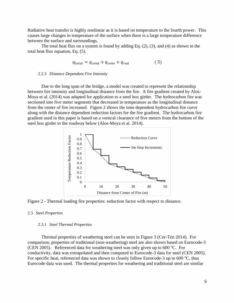
Stress-strain relationships for siliceous and carbonate concrete are shown in Figure 8 and
Figure 9, respectively (CEN 2004). Siliceous concrete was chosen for this research and has a
more rapid loss of strength at elevated temperatures. The direct comparison of reduction in
compression strength can be seen in Figure 10. In addition, Figure 8 and Figure 9 show a linear
relationship between stress and strain up to a level of 0.4 f’c for each temperature level shown. In
Figure 10, the temperature dependent compressive strength reduction is shown for both siliceous
and calcareous concrete.
Figure 8- Temperature dependent stress-strain curves of siliceous concrete.
Figure 9- Temperature dependent stress-strain curves of calcareous concrete.
0
5
10
15
20
25
30
35
0 0.01 0.02 0.03 0.04 0.05
Str
ess
(MP
a)
Strain
20 °C
200 °C
400 °C
600 °C
800 °C
1000 °C
0
5
10
15
20
25
30
35
0 0.01 0.02 0.03 0.04 0.05
Str
ess
(MP
a)
Strain
20 °C
200 °C
400 °C
600 °C
800 °C
1000 °C
11
Figure 10 - Temperature dependent compressive strength of siliceous and calcareous concrete
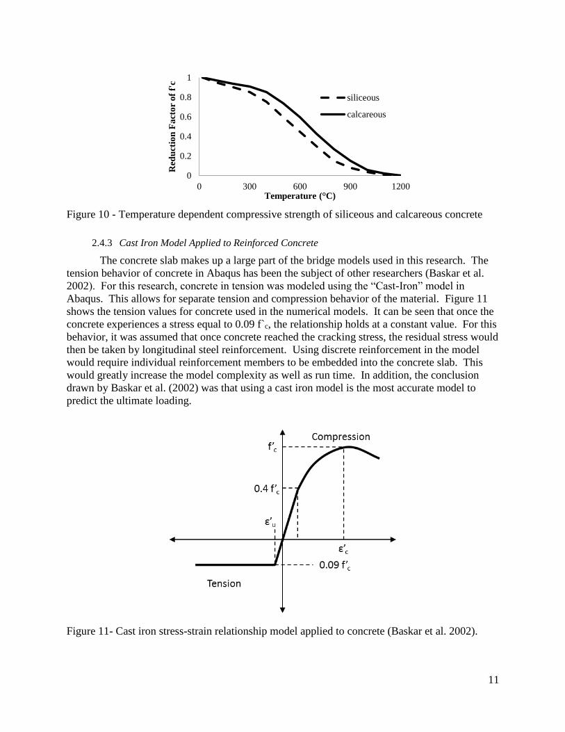
2.4.3 Cast Iron Model Applied to Reinforced Concrete
The concrete slab makes up a large part of the bridge models used in this research. The
tension behavior of concrete in Abaqus has been the subject of other researchers (Baskar et al.
2002). For this research, concrete in tension was modeled using the “Cast-Iron” model in
Abaqus. This allows for separate tension and compression behavior of the material. Figure 11
shows the tension values for concrete used in the numerical models. It can be seen that once the
concrete experiences a stress equal to 0.09 f`c, the relationship holds at a constant value. For this
behavior, it was assumed that once concrete reached the cracking stress, the residual stress would
then be taken by longitudinal steel reinforcement. Using discrete reinforcement in the model
would require individual reinforcement members to be embedded into the concrete slab. This
would greatly increase the model complexity as well as run time. In addition, the conclusion
drawn by Baskar et al. (2002) was that using a cast iron model is the most accurate model to
predict the ultimate loading.
Figure 11- Cast iron stress-strain relationship model applied to concrete (Baskar et al. 2002).
0
0.2
0.4
0.6
0.8
1
0 300 600 900 1200
Red
uct
ion
Fa
cto
r o
f f'
c
Temperature (°C)
siliceous
calcareous

12
2.5 Finite Element Modeling
2.5.1 Hardware/Software
A model of this magnitude and element count requires a high level of computing power
to complete the analysis. The research team is equipped with state-of-art computer hardware and
software. These include a 10-Core Intel Xeon E5-2687W v3 (20 Threads, 25MB Cache, 3.1GHz
Base, 3.5 GHz Turbo) Workstation with 64 GB of 2133MHz DDR4 RAM.
2.5.2 Elements
The 3D models were created using shell elements for the steel tub members and solid
elements for the slab. Shell elements were used to reduce the computational effort which is
important when modeling large, geometrically complex structures through nonlinear analysis.
The bracing used in the model was created using line elements. The shell elements used in the
thermal and structural models are DS4 and S4R. The solid elements used in the thermal and
structural models are 8-noded continuum elements DC3D8 and C3D8R, respectively. The line
elements used for heat transfer were DC1D2. In the structural model, both beam (B31) and truss
(T3D2) elements were used. Figure 12 illustrates the four basic element types that were used in
the Abaqus models.
Figure 12- Basic Element Types (Dassault Systèmes 2013)
2.5.2.1 Heat Transfer Elements
First a thermal model is constructed for the heat transfer analysis. Heat transfer elements
are restricted from all movement and they only consider temperature degrees of freedom.
Material properties assigned to each element includes thermal conductivity, specific heat, and
density.
DS4 – four node, quadrilateral heat transfer shell elements. This element only has degrees of
freedom as defined by the thickness of the element. In this research, shell elements were
given five points along the thickness to define a temperature gradient.
DC3D8 – eight node, linear, solid, diffuse heat transfer elements. This element has one
temperature degree of freedom. This element already is in three dimensions, therefore a
gradient will be shown between nodes.
DC1D2 – two dimensional link elements. Each node is allowed one temperature degree of
freedom (Dassault Systèmes 2013).
13
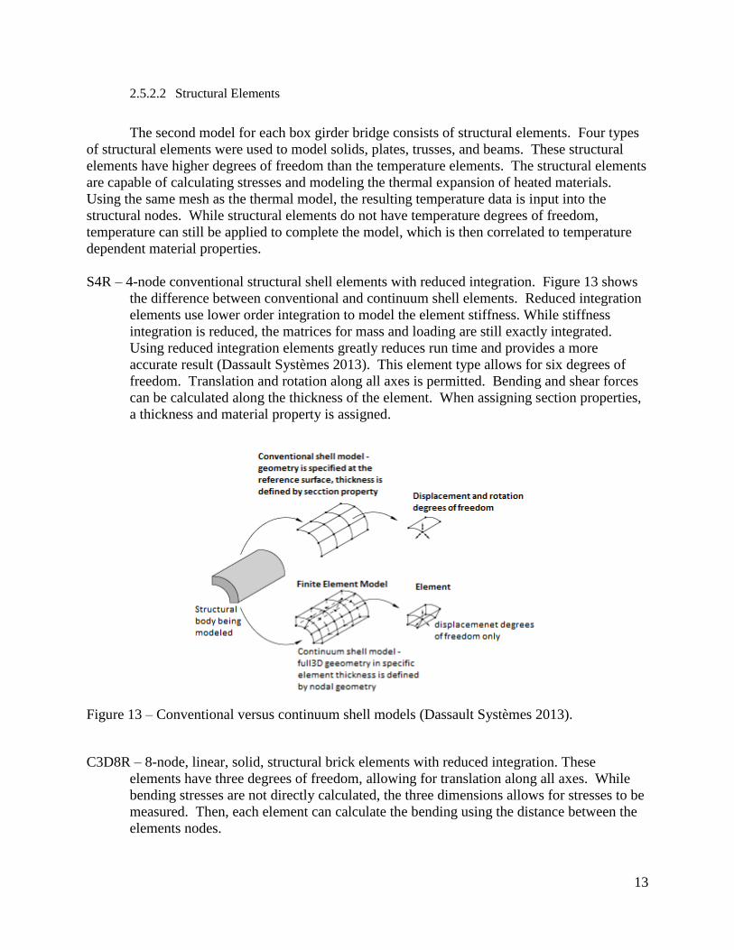
2.5.2.2 Structural Elements
The second model for each box girder bridge consists of structural elements. Four types
of structural elements were used to model solids, plates, trusses, and beams. These structural
elements have higher degrees of freedom than the temperature elements. The structural elements
are capable of calculating stresses and modeling the thermal expansion of heated materials.
Using the same mesh as the thermal model, the resulting temperature data is input into the
structural nodes. While structural elements do not have temperature degrees of freedom,
temperature can still be applied to complete the model, which is then correlated to temperature
dependent material properties.
S4R – 4-node conventional structural shell elements with reduced integration. Figure 13 shows
the difference between conventional and continuum shell elements. Reduced integration
elements use lower order integration to model the element stiffness. While stiffness
integration is reduced, the matrices for mass and loading are still exactly integrated.
Using reduced integration elements greatly reduces run time and provides a more
accurate result (Dassault Systèmes 2013). This element type allows for six degrees of
freedom. Translation and rotation along all axes is permitted. Bending and shear forces
can be calculated along the thickness of the element. When assigning section properties,
a thickness and material property is assigned.
Figure 13 – Conventional versus continuum shell models (Dassault Systèmes 2013).
C3D8R – 8-node, linear, solid, structural brick elements with reduced integration. These
elements have three degrees of freedom, allowing for translation along all axes. While
bending stresses are not directly calculated, the three dimensions allows for stresses to be
measured. Then, each element can calculate the bending using the distance between the
elements nodes.

14
T3D2 – a three dimensional, two node, linear truss element. This element has three degrees of
freedom, allowing for translation along all three axes. Truss elements are used to
approximate elements that only carry axial load. This element cannot carry shear forces
or bending moments. Trusses are created by assigning a cross sectional area and a
material type.
B31 – a three dimensional, two node, linear beam element. This element has six degrees of
freedom allowing for translation and rotation along all three axes. This line element is
used to approximate a three dimensional beam or column member. Each beam is
assigned a cross section and material type. A beam element is capable of three
deformations including axial stretch, bending, and torsion. According to the beam theory
used by Abaqus, the cross section of the beam will remain constant along the length. In
other words, a cross sectional plane will remain the same for the entire beam. This
neglects warping and transverse strains of the cross section (Dassault Systèmes 2013).
2.6 Model validation
2.6.1 Case Study
The finite element modeling procedures were validated against existing test data to
ensure accurate results. An Abaqus model was created to replicate a steel beam and concrete
slab that was subject to increased temperatures. The test, conducted by Wainman et al. (1987),
consisted of heating the beam in a furnace while four point loads were applied at different
locations along the span. The beam had a span of 4.53 m and the dimensions of the concrete and
steel used are shown below. Figure 14 shows a cross section of the beam.
Concrete Slab:
Concrete Quality: CP110:Part1: Grade 30:1972
Width = 635 mm
Depth = 135 mm
Steel Beam:
Steel Quality: BS4360: Grade 43A:1979
Width = 146 mm
Depth = 257 mm
Flange thickness = 12.45 mm
Web thickness = 7.08 mm

15
Figure 14- Cross section of composite beam
Hydraulic jacks applied 32.5 kN to four points located at 1/8, 3/8, 5/8, and 7/8 span.
These loads were applied to the top of the concrete slab before the heating of the specimen.
Once the loads were applied, the beam was subject to increased temperatures. According to the
literature, the exposed length of the beam was 4 meters. Figure 15 shows the arrangement of the
load and supports. The top of the furnace was closed by the concrete slab, therefore, only the
bottom side of the concrete was exposed to direct temperature change. During the test,
temperatures of the beam, the furnace gas, and the midspan deflection were recorded.
Figure 15- Elevation view of beam showing fire application area, supports, and loading points
2.6.2 Model Parameters
2.6.2.1 Thermal Model
To obtain accurate results of the bridge model, the simulation was carried out using
sequential thermal and structural finite element analyses. First a transient, non-linear heat
transfer analysis was performed. Appropriate thermal boundary conditions (radiation and
convection) were applied to the beam in order to obtain a temperature history of the members.
Figure 16 shows the cross section of the beam along with the applied thermal boundary

16
conditions. Radiation boundary conditions require the definition of the emissivity of each fire
exposed surface. The emissivity of the beam surfaces decreases with distance from the source of
the furnace fire. In addition to emissivity, a convection coefficient of 25 W/m2K was used to
replicate the standard fire curve as defined by Eurocode-1 (CEN 2002). This coefficient is used
because the beam is heated in a furnace as opposed to being an open fire scenario.
In order to confirm the validity of the thermal boundary conditions, a two dimensional
model was used to compare the FEM results to the experimental data. A two dimensional model
is beneficial due to the inexpensive nature of the model due to a much lower number of nodes as
compared to the three dimensional model. Once adequate testing was completed, the thermal
boundary conditions were applied to the three dimensional beam. Table 1 shows the resulting
temperatures of the experimental data along with the two dimensional model. Similar
temperatures confirm the initial modeling of the system. Due to the short span of the beam, the
temperature reduction due to horizontal distance from the fire was not used in this modeling.
Figure 16- Cross section of beam showing thermal boundary conditions
Table 1 - Resulting temperatures from Abaqus models and physical model.
Temperatures were recorded at several points on each member of the beam. Figure 17
shows the points on the cross section that were used in analysis. On the top and bottom flange,
temperature was recorded from the bottom face of each flange at the quarter points. For the web,
5 equally spaced points over the web depth were used in the data analysis.
Temperature at 50 Minutes (°C)
Experimental 2-D Abaqus 3-D Abaqus
Top Flange 606 586 (-3.3%) 583 (-3.8%)
Web 749 802 (+7.1%) 813 (+8.5%)
Bottom
Flange 762 812 (+6.6%) 802 (+5.2%)
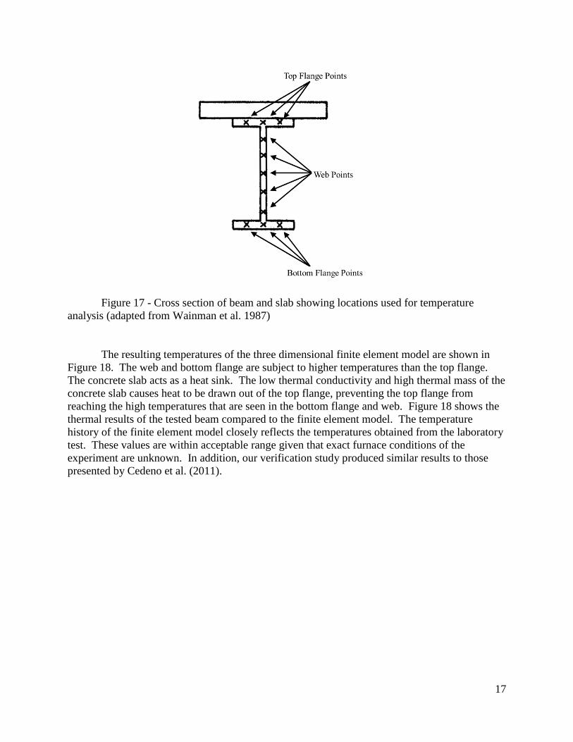
17
Figure 17 - Cross section of beam and slab showing locations used for temperature
analysis (adapted from Wainman et al. 1987)
The resulting temperatures of the three dimensional finite element model are shown in
Figure 18. The web and bottom flange are subject to higher temperatures than the top flange.
The concrete slab acts as a heat sink. The low thermal conductivity and high thermal mass of the
concrete slab causes heat to be drawn out of the top flange, preventing the top flange from
reaching the high temperatures that are seen in the bottom flange and web. Figure 18 shows the
thermal results of the tested beam compared to the finite element model. The temperature
history of the finite element model closely reflects the temperatures obtained from the laboratory
test. These values are within acceptable range given that exact furnace conditions of the
experiment are unknown. In addition, our verification study produced similar results to those
presented by Cedeno et al. (2011).

18
Figure 18 - Comparison of Abaqus data and laboratory test for temperature data.
2.6.2.2 Structural Model
The temperature results output from the thermal analysis are input into a structural model that
will capture the deformation of the beam due to the thermal load. Structural boundary conditions
were set to create a simple span condition. Loading was broken into three steps: (1) self-weight;
(2) point loads; and (3) temperatures. After the self-weight was applied to the model, four 32.5
kN concentrated dead loads were applied, centered around the midpoint of the beam and spaced
at equal intervals along the span length. Finally, the temperatures determined in the heat transfer
model were applied to the structural model. Resulting deflection can be seen in Figure 19 as well
as comparison between the finite element model and the lab test.
0
100
200
300
400
500
600
700
800
900
0 5 10 15 20 25 30 35 40 45
Tem
per
atu
re (
°C)
Time (min)
Mean Furnace Gas
Top Flange-FEM
Web-FEM
Bottom Flange-FEM
Top Flange-Experimental
Web-Experimental
Bottom Flange-Experimental

19
Figure 19 - (a) Comparison of Abaqus data and laboratory test. (b) Abaqus model showing
undeformed steel beam with a concrete slab. (c) Abaqus model showing deflection of a steel
beam with a concrete slab when exposed to fire and loading.
-300
-200
-100
0
0 10 20 30 40
Mid
span
d D
efle
ctio
n (
mm
)
Time (min)
Abaqus Data
Experiment Data
(a)
(b)
(c)

20
3 STRAIGHT BOX GIRDER
3.1 Geometry
3.1.1 Cross Section
During this project, a multi-span, straight steel box girder bridge is subject to sequential
thermal and structural finite element analyses. Dimensions of the bridge follow the U.S.
Department of Transportation FHA Steel Bridge Design Handbook (FHWA 2012a). Figure 20
shows a section of the Abaqus bridge model including transverse web stiffeners. The steel has a
total cross section area of 0.288 square meters. The slab has an approximate cross sectional area
of 1.5 square meters. The cross sectional dimensions of the bridge can be seen in Figure 22.
The entire model can be seen in Figure 21 In order to limit model size, only a single box girder
section is considered.
Figure 20 - Cross section of straight box girder bridge Abaqus model.
Figure 21 - Full straight box girder bridge model.

21
Figure 22 - Cross sectional dimensions of the straight steel box girder bridge (FHWA 2012a).
Elevation
Figure 23 shows an elevation view of the bridge that indicates the plate thicknesses along
the bridge span. Thickness of flange plates increase closer to the bridge pier. The web is
constant along the length of the bridge. The bridge has a total length of 198.12 meters with two
symmetrical interior piers. The two outer spans each measure 57.15 meters and the middle span
measures 83.82 meters in length. The stiffeners used in this model were made from weathering
steel that was 0.222 m wide and 0.019 m thick.
Figure 23 - Elevation view of the straight box girder bridge showing plate thickness and location.
Intermediate web transverse stiffeners are not shown for clarity (FHWA 2012a).
3.1.2 Internal Bracing
In addition to the steel tub and concrete slab, the bridge model included many bracing
elements. Figure 24 shows the plan view of the internal bracing for the bridge. The bracing is
composed of angle (L) members with a thickness of .0095 m and each side of the L being 0.127
m in length (L0.127x0.127x0.0095). The bracing was attached to the cross-section of the bridge
at the stiffeners.

22
Figure 24 - Framing plan of the straight bridge showing view of all bracing members (FHWA
2012a).
3.2 Finite Element Model
The bridge model was constructed using multiple element types. The concrete slab was
modeled using 20,740 solid (C3D8R) elements and the steel tub was made of 13,381 shell (S4R)
elements. In addition, 90 truss (T3D2) and 540 beam (B31) elements were used to model the
bracing. The use of shell elements was implemented to reduce the overall run time but still
maintain a high level of accuracy. The line elements that spanned the bridge horizontally and
perpendicular to the bridge span were beam elements. Beams were used to allow additional
cross members to be attached and allow bending. Diagonal cross bracing and vertical bracing
was made of truss elements. These truss elements are able to free rotate at each end but may
only resist axial forces. Once constructed, the model contained a total of 48,751 nodes.
3.3 Fire Scenarios and Thermal Boundary Conditions
Hydrocarbon fires are considered for this research. Two fire locations have been
modeled in this research. The first fire is located in the center of the middle span. Fire location
1 represents the farthest distance from any of the bridge piers. Figure 25 shows the fire location
and fire reduction curve associated with the midspan fire. Fire location 2 corresponds to the area
adjacent to an inner pier. This fire location represents the closest the fire can be to a support.
Figure 26 shows the pier fire location along with the fire reduction curve.
In initial testing, a two hour fire was used on the box girder bridge model. However, a
two hour fire was not required to reach the full model runtime of the bridge model. In order to
greatly reduce computation time, 30 minutes of fire was modeled in the straight bridge model as
failure occurs much sooner than two hours. In the event of the structural model running the full
30 minutes of fire, this time would have been extended. However, it will be shown that 30
minutes of fire was adequate for this model.

23
Figure 25 - Midspan fire location of the straight bridge with fire reduction curve
Figure 26 - Pier fire location of the straight bridge with fire reduction curve

24
The plate thicknesses shown in Figure 23 indicate that the bottom flange of the bridge at
fire location 2 is much thicker than the bottom flange at fire location 1. This is important
because a member with a larger thickness will have a larger weight-to-heated perimeter (W/D)
ratio. Members with larger weight-to-heated perimeter ratios will inherently have a greater
resistance to temperature increase due to fire. A larger weight of the member will slow the heat
transfer within the member as greater energy is required to raise the temperature. Additionally,
a smaller heated perimeter implies less surface area exposed to the fire and thus less heat
entering into the member. Therefore, the bottom flange at fire location 2 is expected to change
temperature at a slower rate than the bottom flange at fire location 1.
Figure 27 shows the thermal boundary conditions applied in the heat transfer model –
convection and radiation. According to Eurocode, the convection coefficient for a hydrocarbon
fire is taken to be 50 W/m2K for the fire exposed surfaces. A convection coefficient of 9 W/m2K
is applied to the non-exposed surfaces to account for heat loss from the top of the bridge section
into the ambient air above the bridge that is not affected by the fire. For the radiative thermal
boundary condition, the resultant emissivity between the fire surface and the bridge surface is
defined. The emissivity of the fire is taken as 1.0 (CEN 2002). Due to the large depth of the
cross section of the bridge, the emissivity value will decrease with vertical distance from the fire.
The emissivity of the bottom flange, web, top flange and slab are 0.7, 0.5, 0.3, and 0.3
respectively based on recommendations from Kodur et al. (2013).
Figure 27 - Convection and emissivity values used in the thermal model

25
3.4 Structural Boundary Conditions
Figure 28 shows the support conditions for the straight box girder bridge in all three
directions. Rollers are placed at support A, C, and D. These allow for movement in the x-axis,
and restricts movement in the y-axis and z-axis. Also, rotation is restricted about the y-axis and
x-axis, allowing only for moment about the z-axis. A pin is used at support B. At this support,
no translational movement is allowed. Moment is allowed about the z-axis and restricted about
the y-axis and x-axis.
Figure 28- Support conditions of the straight box girder bridge with arrows showing free
displacement.
3.5 AASHTO Design Requirements
3.5.1 Shear Resistance
Section 6.10.9 of the AASHTO Bridge Design Specifications outlines the strength limit
state of web panels. This section includes straight, curved, stiffened, and unstiffened panels. For
all panels, the general equation for shear resistance, shown in Eq. (6), must be satisfied. It
should be noted that Section 6.10.9 is for I-sections. However, Section 6.11.9 states that that
Section 6.10.9 should be used for web shear resistance of tub sections.
𝑉𝑢 ≤ 𝜑𝑣𝑉𝑛 (6) 𝑤ℎ𝑒𝑟𝑒: 𝜑𝑣 = 𝑟𝑒𝑠𝑖𝑠𝑡𝑎𝑛𝑐𝑒 𝑓𝑎𝑐𝑡𝑜𝑟 𝑉𝑛 = 𝑛𝑜𝑚𝑖𝑛𝑎𝑙 𝑠ℎ𝑒𝑎𝑟 𝑟𝑒𝑠𝑖𝑠𝑡𝑎𝑛𝑐𝑒 𝑉𝑢 = 𝑠ℎ𝑒𝑎𝑟 𝑖𝑛 𝑤𝑒𝑏

26
The nominal shear resistance of an interior stiffened web panel is shown in Eq. (7).
𝑉𝑛 = 𝑉𝑝
[
𝐶 +0.87 (1 − 𝐶)
√1 + (𝑑0
𝐷 )2
]
(7)
𝑤ℎ𝑒𝑟𝑒: 𝑑0 = 𝑡𝑟𝑎𝑛𝑠𝑣𝑒𝑟𝑠𝑒 𝑠𝑡𝑖𝑓𝑓𝑒𝑛𝑒𝑟 𝑠𝑝𝑎𝑐𝑖𝑛𝑔 𝑉𝑝 = 𝑝𝑙𝑎𝑠𝑡𝑖𝑐 𝑠ℎ𝑒𝑎𝑟 𝑓𝑜𝑟𝑐𝑒
𝐶 = 𝑟𝑎𝑡𝑖𝑜 𝑜𝑓 𝑡ℎ𝑒 𝑠ℎ𝑒𝑎𝑟 − 𝑏𝑢𝑐𝑘𝑙𝑖𝑛𝑔 𝑟𝑒𝑠𝑖𝑠𝑡𝑎𝑛𝑐𝑒 𝑡𝑜 𝑠ℎ𝑒𝑎𝑟 𝑦𝑖𝑒𝑙𝑑 𝑠𝑡𝑟𝑒𝑛𝑔𝑡ℎ
And the plastic shear force is found using Eq. (8).
𝑉𝑝 = 0.58𝐹𝑦𝑤𝐷𝑡𝑤 (8)
𝑤ℎ𝑒𝑟𝑒: 𝐹𝑦𝑤 = 𝑠𝑡𝑒𝑒𝑙 𝑦𝑖𝑒𝑙𝑑 𝑠𝑡𝑟𝑒𝑛𝑔𝑡ℎ
𝐷 = 𝑑𝑒𝑝𝑡ℎ 𝑜𝑓 𝑤𝑒𝑏 𝑡𝑤 = 𝑡ℎ𝑖𝑐𝑘𝑛𝑒𝑠𝑠 𝑜𝑓 𝑤𝑒𝑏
The ratio of the shear buckling resistance to the shear yield strength is determined by the Eq. (9)
through Eq. (11).
𝐼𝑓 𝐷
𝑡𝑤≤ 1.12√
𝐸𝑘
𝐹𝑦𝑤, 𝑡ℎ𝑒𝑛
𝐶 = 1.0 (9)
𝐼𝑓 1.12√𝐸𝑘
𝐹𝑦𝑤<
𝐷
𝑡𝑤≤ 1.40√
𝐸𝑘
𝐹𝑦𝑤, 𝑡ℎ𝑒𝑛
𝐶 =1.12
𝐷𝑡𝑤
√𝐸𝑘
𝐹𝑦𝑤 (10)
𝐼𝑓 𝐷
𝑡𝑤> 1.40√
𝐸𝑘
𝐹𝑦𝑤, 𝑡ℎ𝑒𝑛
𝐶 =1.57
(𝐷𝑡𝑤
)2 (
𝐸𝑘
𝐹𝑦𝑤) (11)
𝑤ℎ𝑒𝑟𝑒: 𝑘 = 𝑠ℎ𝑒𝑎𝑟 𝑏𝑢𝑐𝑘𝑙𝑖𝑛𝑔 𝑐𝑜𝑒𝑓𝑓𝑖𝑐𝑖𝑒𝑛𝑡

27
Eq. (12) shows the calculation for the shear buckling coefficient.
𝑘 = 5 + 5
(𝑑0
𝐷 )2 (12)
3.5.2 Moment Capacity
When investigating the moment capacity of the box girder bridges, the bridge cross
section can be analyzed in the same fashion as other composite cross-sections by using plastic
analysis. Figure 29 shows a cross section of the box girder showing associated tension and
compression forces that are produced in positive bending at the fully plastic condition.
Figure 29 – Plastic analysis with stress block in the flange
Members located above the neutral axis will be in compression while members below the
neutral axis will be in tension when positive bending is present. To achieve equilibrium, the
tension and compression forces must balance. By setting each equation equal, we can solve for
a, which is the depth of the compression stress block. Eq. 13 shows this resulting formula, for
the case when a≤tf.
𝑎(𝑇) = ∑𝑇𝑒𝑛𝑠𝑖𝑙𝑒 𝐹𝑜𝑟𝑐𝑒𝑠
0.85𝑓′𝑐(𝑇)𝑏𝑒𝑓𝑓
(13)
The temperature dependent yield strength, Fy(T), is found from Figures 4 and 5 while the
temperature dependent concrete compressive strength, f’c(T), is found from Figure 8 and 9.
Therefore, a becomes temperature (and therefore time) dependent, and denoted as a(T).
The stress block may extend down to within the slab, the top flange, or in the web,
depending on the properties of the cross-section. Assuming that it is within the concrete slab
before heating, as shown on Figure 28, an increase in temperature will affect the location. It was

28
previously established in Figure 4 that the strength of weathering steel is reduced with an
increase in temperature. Therefore, if the yield strength of the steel in Figure 28 is reduced, a
will also be reduced. It should be noted that the compression strength of the concrete is also
reduced with increased temperature, but the distance of the slab from the fire is much greater
than the steel components of the box girder. As a result, the slab remains considerably cooler
and reduces strength at a lower rate. As the term a decreases, the neutral axis of the system
moves upward into the concrete slab. This results in a lower amount of concrete in compression
which further results in a lower moment capacity. As time progresses, the moment capacity of
the bridge continues to decreases and the moment demand remains the same.
A simplified model, considering the tensile yield stress of the bottom flange has also been
considered. The moment capacity is calculated from the traditional beam bending stress
equation, assuming the bottom flange (closest to the fire) tensile stress controls. Eq. 14
illustrates the moment capacity as a function of temperature:
𝑀(𝑇) = 𝐹𝑦(𝑇) ∗ 𝑆𝑥−𝑏𝑓 (14)
Where Sx-bf indicates the elastic section modulus with respect to the bottom flange.
3.6 Heat Transfer Results
First, the heat transfer analysis was performed on the box girder bridge. Maximum
temperature histories were recorded at four locations shown in Figure 30. One node was selected
from the center of the heated face of the bottom flange, web, top flange, and exposed slab. Due
to the fire gradient, only one node is needed because each element has the same surface
temperature history in each gradation. Figure 31 shows a plot of element temperatures versus
time for both fire locations. At the central location, the bottom flange had a thickness of 0.0143
meters. This flange thickness is the lowest of all steel elements. Moreover, the cross section at
this location has the lowest weight-to-heated perimeter ratio. The bottom flange temperature of
fire location 2 is lower than that of the fire location 1. This is because the bottom flange
thickness is 0.0413 meters, almost three times the thickness of the bottom flange plate at
midspan of the bridge. The bridge cross section at fire location 2 also corresponds to the highest
weight-to-heated perimeter ratio of all of the cross-sections. This is because the sizes of the top
and bottom flange plates are each at their maximum at the bridge pier location.
In addition to the temperatures in the shell elements, Figure 32 shows the temperature of
the center node of the interior bracing line element. This represents the line element directly
over the full strength fire. This figure shows that the interior line elements remain at a low
temperature and will not see the effect of reduced strength due to increased temperature.
Therefore, the line elements have been removed from the thermal model and there is no
temperature change in the structural model. This allows for a savings in model run time.
29
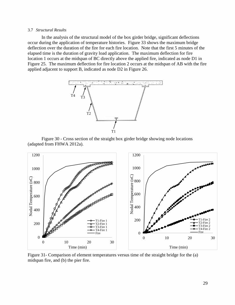
3.7 Structural Results
In the analysis of the structural model of the box girder bridge, significant deflections
occur during the application of temperature histories. Figure 33 shows the maximum bridge
deflection over the duration of the fire for each fire location. Note that the first 5 minutes of the
elapsed time is the duration of gravity load application. The maximum deflection for fire
location 1 occurs at the midspan of BC directly above the applied fire, indicated as node D1 in
Figure 25. The maximum deflection for fire location 2 occurs at the midspan of AB with the fire
applied adjacent to support B, indicated as node D2 in Figure 26.
Figure 30 - Cross section of the straight box girder bridge showing node locations
(adapted from FHWA 2012a).
Figure 31- Comparison of element temperatures versus time of the straight bridge for the (a)
midspan fire, and (b) the pier fire.
T1
T2
T3T4
0
200
400
600
800
1000
1200
0 10 20 30
Nodal
Tem
per
ature
(oC
)
Time (min)
T1-Fire 1T2-Fire 1T3-Fire 1T4-Fire 1Fire 0
200
400
600
800
1000
1200
0 10 20 30
Nodal
Tem
per
ature
(oC
)
Time (min)
T1-Fire 2T2-Fire 2T3-Fire 2T4-Fire 2Fire

30
As expected, maximum deflection for fire location 1 (at node D1 at midspan of BC) was much
larger than the maximum deflection for fire location 2 (at node D2 at midspan AB) due to
proximity of the fire to the bridge support in fire location 2. Deflection at node D1 due to fire
location 2 and node D2 due to fire location 1 are minimal as the fire is applied at a distance away
from the D1 and D2, respectively, on different spans. Figure 35 and Figure 35 show the
amplified deflected shape for each fire location, from the Abaqus model.
Figure 32- Temperature of the line element directly over the full strength fire
Figure 33- Comparison of maximum bridge deflection of the straight box girder bridge.
-0.6
-0.5
-0.4
-0.3
-0.2
-0.1
0
0 5 10 15 20
Ver
tica
l D
efle
ctio
n (
m)
Elapsed Time (min)
Fire Location 1
Fire Location 2
5 min
0
5
10
15
20
25
0 20 40 60 80 100 120 140
Nodal
Tem
per
atu
re (
oC
)
Time (min)

31
For fire location 2, the Abaqus model runs for 17.1 minutes. Maximum deflection occurs
at approximately the mid-point of the Span A-B (Figure 25). Minimal vertical deflection is seen
at the location of the fire because the boundary conditions prevent movement in the vertical
direction. However, shear demand is greatest directly adjacent to the support at node D2.
Figure 38 shows maximum deflection for node D2 for fire location 2 over the duration of
the fire along with the ratio of the shear demand of the girder to the nominal shear capacity of the
section at that location. Nominal shear capacity of the section was calculated based on
AASHTO Bridge Design Specifications (2012) with adjustments made to account for
temperature dependent (reduced) steel yield strength and elastic modulus based on the average
temperature in the web of the girder over the duration of the fire. Eq. 8 shows that yield strength
of steel determines the shear resistance. As yield strength decrease with time, shear resistance
also decreases. Shear demand was calculated based on dead load only to be 1700 kN at location
D2. The shear demand reaches the shear capacity of the girder at approximately 17 minutes into
the fire, correlating precisely to the 17.1 minutes that the Abaqus model was able to run.
Therefore, it is the authors’ conclusion that for the box girder presented in this paper when the
fire is applied adjacent to the support (fire location 2) the bridge failed at 17.1 minutes into the
fire due to shear buckling of the web. Figure 36 shows a section above fire location 2. The
stresses in the web are much lower than surrounding members due to the increase in temperature.
For fire location 1, deflection increases rapidly once the temperature histories are applied.
The maximum global deflection occurs at the same location as the fire. Maximum displacement
occurs at 11.1 minutes. Web shear failure is not the mode of failure in this instance. This is
because the shear demand at the mid span is much lower (near zero) than at fire location 2. Also,
web temperatures are the same so there is not a difference in shear capacity. However, the
deflection at location D1, there is a buildup of stresses in the bottom flange. At this location, the
moment will be at its maximum due to dead load only. In addition, the stresses due to the
moment will be greatest along the bottom most member of the bridge. Moment demand at mid
span for fire location 1 was calculated to be 15473 kN-m. Figure 37 shows a section above fire
location 1. The underside of the bridge is picutred to show that the bottom flange of the bridge
can no longer hold significant stress due to the loss of strength in high temperature.
Figure 39 shows maximum deflection for node D1 for fire location 1 over the duration of
the fire along with the ratio of the moment demand (due to dead load only) of the girder at that
location to the nominal moment capacity of the section. The moment capacity is based on
tension flange yielding calculated using reduced yield strength based on the average temperature
of the bottom flange over the duration of the fire. Similarly to yield strength, the moment
resistance of the bridge is reduced as yield strength of the bottom flange decreases as shown in
section 3.5.2. Maximum displacement occurs at 11.1 minutes and the demand to capacity ratio
reaches 1 at 12.9 minutes, using the simplified capacity calculation. Using the full plastic
analysis, the demand to capacity ratio reaches 1 at approximately 15 minutes. This provides a
larger discrepancy from the run time of the Abaqus model. The authors believe there are some
additional local effects that need to be considered to account for this difference.

32
Figure 34 - Deflected shape and Mises stress of the straight box girder bridge corresponding to
fire location 1.
Figure 35 - Deflected shape and Mises stress of the straight box girder bridge corresponding to
fire location 2.

33
Figure 36 – Final step of analysis corresponding to fire location 2.
Figure 37 - Final step of analysis corresponding to fire location 1.
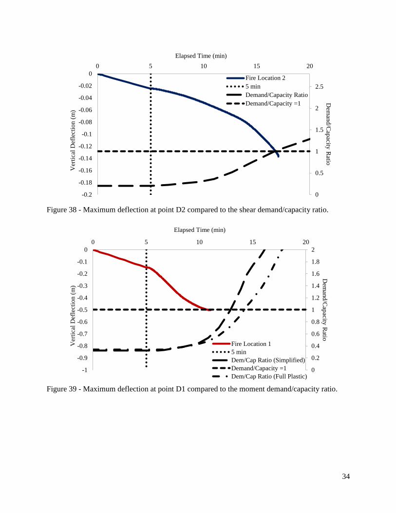
34
Figure 38 - Maximum deflection at point D2 compared to the shear demand/capacity ratio.
Figure 39 - Maximum deflection at point D1 compared to the moment demand/capacity ratio.
0
0.2
0.4
0.6
0.8
1
1.2
1.4
1.6
1.8
2
-1
-0.9
-0.8
-0.7
-0.6
-0.5
-0.4
-0.3
-0.2
-0.1
0
0 5 10 15 20
Dem
and
/Cap
acity R
atioV
erti
cal
Def
lect
ion (
m)
Elapsed Time (min)
Fire Location 1
5 min
Dem/Cap Ratio (Simplified)
Demand/Capacity =1
Dem/Cap Ratio (Full Plastic)
0
0.5
1
1.5
2
2.5
-0.2
-0.18
-0.16
-0.14
-0.12
-0.1
-0.08
-0.06
-0.04
-0.02
0
0 5 10 15 20D
eman
d/C
apacity
Ratio
Ver
tica
l D
efle
ctio
n (
m)
Elapsed Time (min)
Fire Location 2
5 min
Demand/Capacity Ratio
Demand/Capacity =1

35
3.8 End Restraint Investigation
In addition to the model explained above, an investigation was performed using different
end conditions in order to analyze the effect of end restraints. Figure 40 shows the alteration of
support conditions. The bridge abutment support D was made a pin support allowing only for
rotation in the x-y plane.
Figure 41 shows the deflection of both fire locations 1 and 2 with each support condition.
It can be seen that for fire location 1 (midspan) the effect of the end restraint was minimal. The
suffix “ER” in the figure indicates the model with the additional end restraint at D. The model
with additional end restraint ran for 9.75 minutes with a total deflection of 0.5 m. This is
approximately a 1.5 minute difference in run time with the final deflection being equal.
For the pier fire case, Figure 41 shows the end restraint condition alters the results of the
structural model. The maximum deflection of 0.28 m is reached after a total run time of 23.25
minutes. This deflection is 0.14 m larger and the model runs 6.1 minutes longer than then model
without the additional end restraint condition.
Table 2 shows a summary of the resulting data for the two fire locations applied to the
straight box girder bridge.
Figure 40 - Support conditions of the straight box girder bridge with additional end restraint.

36
Figure 41 - Vertical deflection of the straight steel box girder bridge with two different support
conditions.
Table 2 - Resulting deflection data for the straight box girder bridge different end restraint
conditions
Run Time (min) Max Deflection (m)
Fire location 1:
Mid Span Fire
Original End Restraint 11.1 0.5
Modified End Restraint 9.75 0.5
Fire location 2:
Pier Fire
Original End Restraint 17.1 0.14
Modified End Restraint 23.25 0.28
-1
-0.9
-0.8
-0.7
-0.6
-0.5
-0.4
-0.3
-0.2
-0.1
0
0 5 10 15 20 25
Ver
tica
l D
efle
ctio
n (
m)
Elapsed Time (min)
Fire Location 1
Fire Location 1 ER
Fire Location 2
Fire Location 2 ER
5 min

37
4 CURVED BOX GIRDER
4.1 Geometry
4.1.1 Cross Section
Dimensions of the curved bridge follow the U.S. Department of Transportation FHA
Steel Bridge Design Handbook (FHWA 2012b). The cross sectional geometry of the bridge is
similar to the straight model shown in section 3 of this report. Figure 42 shows one section of
the bridge that is located over one of the interior bridge supports. The steel has a total cross
section area of 0.218 square meters. The slab has an approximate cross sectional area of 1.5
square meters. Figure 43 shows a cross section cut of the finite element model and Figure 44
shows the full model.
Figure 42 – Cross sectional dimensions of the curved steel box girder bridge (FHWA 2012b).
Figure 43 – - Cross section of curved box girder bridge Abaqus model.

38
Figure 44 –Full curved box girder bridge model.
4.1.2 Elevation
Figure 45 shows an elevation view of the bridge that indicates plate thickness along the
bridge span. Thickness of flange plates increase closer to the bridge pier. The web is constant
along the length of the bridge. The bridge has a total length of 161.54 meters with two
symmetrical interior piers. The two outer spans each measure 48.77 meters and the middle span
measures 64.01 meters in length.
Figure 45-Elevation view of the curved box girder bridge showing plate thickness and location
(FHWA 2012b).

39
4.1.3 Framing
Figure 46 shows the plan view of the framing of the curved box girder bridge. The radius
of the bridge is 216.79 meters.
Figure 46 - Plan view of the curved box girder bridge showing framing.
4.2 Finite Element Model
The curved bridge model was constructed using multiple element types. The concrete
slab was modeled using 14,996 solid (C3D8R) elements and the steel tub was made of 10,254
shell (S4R) elements. In addition, 70 truss (T3D2) and 210 beam (B31) elements were used to
model the bracing. The use of shell elements was implemented to reduce the overall run time but
still maintain a high level of accuracy. The line elements that spanned the bridge horizontally
and perpendicular to the bridge span were beam elements. Beams were used to allow additional
cross members to be attached and allow bending. Diagonal cross bracing and vertical bracing
was made of truss elements. Once constructed, the model contained a total of 34,559 nodes.
The difference in node count from the straight model is a combination of the smaller cross
sectional area and shorter length. The curved bridge model is approximately 30 meters shorter
and has a cross sectional area that is 0.067 square meters less than the straight model.
4.3 Fire Scenario and Location
The same fire curve used in the straight box girder was used in the curved model. This
curve can be seen in section 2 of this report. As with the straight box model, a two hour fire was
not required to reach the full model runtime of the curved bridge. In the event of the structural
model running the full 30 minutes of fire, this time would have been extended. However, it will
be shown that 30 minutes of fire was adequate for this model.

40
Figure 47- Midspan fire location of curved bridge with fire reduction curve.
Figure 48 - Pier fire location of curved bridge with fire reduction curve.
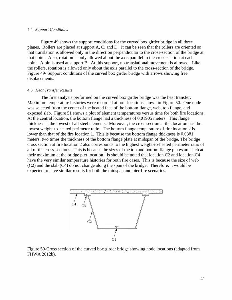
41
4.4 Support Conditions
Figure 49 shows the support conditions for the curved box girder bridge in all three
planes. Rollers are placed at support A, C, and D. It can be seen that the rollers are oriented so
that translation is allowed only in the direction perpendicular to the cross-section of the bridge at
that point. Also, rotation is only allowed about the axis parallel to the cross-section at each
point. A pin is used at support B. At this support, no translational movement is allowed. Like
the rollers, rotation is allowed only about the axis parallel to the cross-section of the bridge.
Figure 49- Support conditions of the curved box girder bridge with arrows showing free
displacements.
4.5 Heat Transfer Results
The first analysis performed on the curved box girder bridge was the heat transfer.
Maximum temperature histories were recorded at four locations shown in Figure 50. One node
was selected from the center of the heated face of the bottom flange, web, top flange, and
exposed slab. Figure 51 shows a plot of element temperatures versus time for both fire locations.
At the central location, the bottom flange had a thickness of 0.01905 meters. This flange
thickness is the lowest of all steel elements. Moreover, the cross section at this location has the
lowest weight-to-heated perimeter ratio. The bottom flange temperature of fire location 2 is
lower than that of the fire location 1. This is because the bottom flange thickness is 0.0381
meters, two times the thickness of the bottom flange plate at midspan of the bridge. The bridge
cross section at fire location 2 also corresponds to the highest weight-to-heated perimeter ratio of
all of the cross-sections. This is because the sizes of the top and bottom flange plates are each at
their maximum at the bridge pier location. Is should be noted that location C2 and location C4
have the very similar temperature histories for both fire cases. This is because the size of web
(C2) and the slab (C4) do not change along the span of the bridge. Therefore, it would be
expected to have similar results for both the midspan and pier fire scenarios.
Figure 50-Cross section of the curved box girder bridge showing node locations (adapted from
FHWA 2012b).

42
(a) (b)
Figure 51- Element temperatures verses time of the curved box girder bridge for the (a) midspan
fire, and (b) the pier fire.
4.6 Structural Results
In the analysis of the structural model of the curved box girder bridge, the results have
several similarities to the results of the straight box girder bridge. The maximum vertical
deflection resulting from the two fire applications can be seen in Figure 52. As with the straight
box girder bridge, the first 5 minutes of the elapsed time is the duration of gravity load
application. The maximum deflection for fire location 1 occurs at the midspan of BC directly
above the applied fire, indicated as node D1 in Figure 25. The maximum deflection for fire
location 2 occurs at the midspan of AB with the fire applied adjacent to support B, indicated as
node D2 in Figure 48. Figure 53 and Figure 54 illustrate the final deflected shape of each bridge
model. Note that vertical deflections are exaggerated for clarity.
When the pier fire is applied to the curved bridge, the Abaqus model runs for 18.25
minutes. In this scenario, maximum deflection occurs at a distance away from the fire which is
shown in Figure 48. Minimal vertical deflection is seen at the location of the fire because of the
proximity to the support which prevents deflection. The deflection that is observed in this case
produces the greatest shear demand directly adjacent to the support at location D2.
In Figure 57, the deflection of the bridge is compared to the ratio of the shear demand to
nominal shear capacity. Shear capacity is calculated at the location of maximum shear. The
0
200
400
600
800
1000
1200
0 10 20 30
No
dal
Tem
per
atu
re (
°C)
Time (min)
C1-Fire 1
C2-Fire 1
C3-Fire 1
C4-Fire 1
Fire
0
200
400
600
800
1000
1200
0 10 20 30N
od
al T
emp
erat
ure
(°C
)Time (min)
C1-Fire 2C2-Fire 2C3-Fire 2C4-Fire 2Fire

43
shear capacity is adjusted based on the decrease in yield strength of the steel. In section 3.5.1 the
AASHTO Bridge Design Specification for shear capacity are shown. The shear demand at this
location was found to be 1380 kN due to gravity load. Shear capacity becomes equal to shear
demand at approximately 16.5 minutes. This is compared to an Abaqus model run time of 18.25
minutes. Therefore, the model runs slightly longer than would be predicted by the demand to
capacity ratio. However, it can be seen that once the demand to capacity ratio exceeds one, the
deflection rapidly decreases until the model ends. Figure 55 shows a section above fire location
1. The stresses in the web are much lower than surrounding members due to the increase in
temperature.
The maximum deflection for the midspan fire (location 1) resulted in a larger deflection
then the fire adjacent to the bridge pier (location 2). As with the straight model, this is due to the
proximity of fire location 2 to the support of the bridge. Deflection at node D1 due to fire
location 2 and node D2 due to fire location 1 are minimal as the fire is applied at a distance away
from the D1 and D2, respectively, on different spans.
The bridge model that represents fire location 1 has a sudden increase in deflection once
the fire is applied. The maximum deflection occurs at the same location as the application of
fire. At this location, the positive moment demand is the largest. Maximum deflection occurs at
9.5 minutes of runtime. The final deflection of the bridge is 0.29 m.
Figure 58 shows a plot of vertical deflection of the bridge along with the ratio of moment
demand to nominal moment capacity. As explained in section 3.5.2, as the bottom flange
temperature increases, the yield strength of the steel is reduced resulting in a reduced moment
capacity. The moment demand at this location was found to be 6593 kN-m. Using the
simplified moment capacity calculation, the demand to capacity ratio exceeds 1 at approximately
17 minutes. The ratio between demand and capacity exceeds 1 at approximately 11.5 minutes
according to the full plastic moment capacity calculations. This is two minutes longer than the
model run time and shows that using the full plastic analysis in this case, produces more
favorable results of correlation with model run time. Figure 56 shows a section above fire
location 1. The underside of the bridge is picutred to show that the bottom flange of the bridge
can no longer hold significant stress due to the loss of strength in high temperature.
-0.3
-0.25
-0.2
-0.15
-0.1
-0.05
0
0 5 10 15 20
Ver
tica
l D
efle
ctio
n (
m)
Elapsed Time (min)
Fire Location 1
Fire Location 2
5 min

44
Figure 52-Comparison of maximum deflection of the curved box girder bridge.
Figure 53- Deflected shape and Mises stress of the curved box girder bridge corresponding to
fire location 2.
Figure 54 - Deflected shape and Mises stress of the curved box girder bridge corresponding to
fire location 1.

45
Figure 55 - Final step of analysis corresponding to fire location 2.
Figure 56- Final step of analysis corresponding to fire location 1.
Figure 57- Maximum deflection at point D2 compared to the shear demand/capacity ratio
0
0.5
1
1.5
2
2.5
3
-0.29
-0.25
-0.21
-0.17
-0.13
-0.09
-0.05
-0.01
0 2 4 6 8 10 12 14 16 18 20 22 24
Dem
and
/Cap
acity R
atioVer
tica
l D
efle
ctio
n (
m)
Elapsed Time (min)
Fire Location 2
5 min
Demand/Capacity Ratio
Demand/Capacity = 1

46
Figure 58 - Maximum deflection at point D1 compared to the moment demand/capacity ratio
4.7 End Restraint Investigation
As with the straight box girder, support conditions were modified to observe any change
to the results that would occur by adding additional end restraints. Figure 59 shows the support
conditions that were used to compare to the support conditions mentioned earlier in this section.
In the additional end restraint model (“ER”), point D is no longer free tangentially, but instead
resists displacement.
Figure 60 shows the results of both support condition models related to the two fire
location scenarios. For fire location 1 with end restraint, the model reaches a maximum
deflection of 0.28 m at a final time of 9.25 minutes. This represents a 15 second shorter run time
and a .01 m difference in vertical deflection compared to the model without end restraints.
For fire location 2, it can be seen that the Abaqus model runs for the same amount of time with a
difference in deflection of 0.01 m. Table 3 shows a summary of the resulting data for each
restraint condition. Comparing the results for the straight and curved box girder illustrates that
the additional restraint at D is more critical to the performance of the straight alignment. The
stability provided by the additional restraint is beneficial, as it allows for a longer runtime before
failure.
0
0.5
1
1.5
2
2.5
-0.5
-0.45
-0.4
-0.35
-0.3
-0.25
-0.2
-0.15
-0.1
-0.05
0
0 2 4 6 8 10 12 14 16 18
Dem
and
/Cap
acity R
atioVer
tica
l D
efle
ctio
n (
m)
Elapsed Time (min)
Fire Location 1
5 mins
Dem/Cap Ratio (Simplified)
Demand/Capacity = 1
Dem/Cap Ratio (Full Plastic)
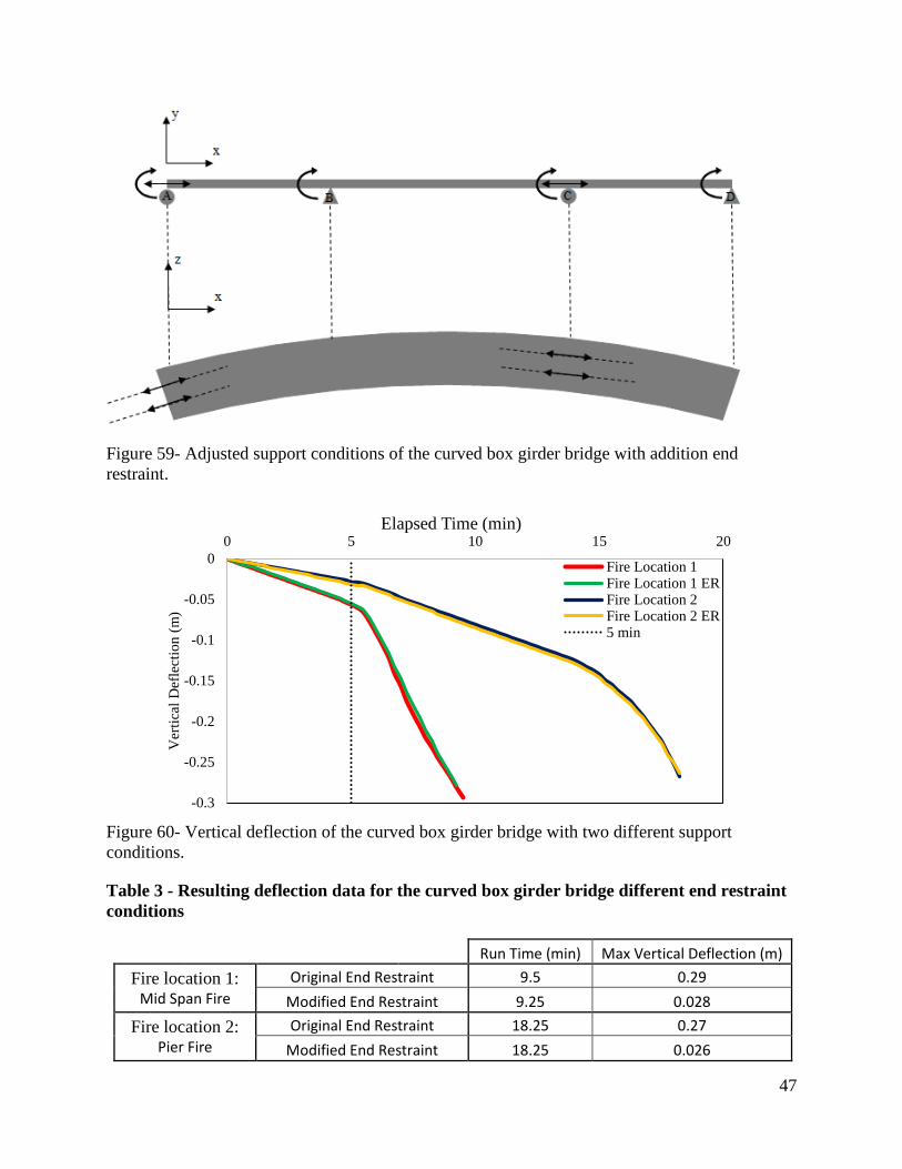
47
Figure 59- Adjusted support conditions of the curved box girder bridge with addition end
restraint.
Figure 60- Vertical deflection of the curved box girder bridge with two different support
conditions.
Table 3 - Resulting deflection data for the curved box girder bridge different end restraint
conditions
Run Time (min) Max Vertical Deflection (m)
Fire location 1: Mid Span Fire
Original End Restraint 9.5 0.29
Modified End Restraint 9.25 0.028
Fire location 2: Pier Fire
Original End Restraint 18.25 0.27
Modified End Restraint 18.25 0.026
-0.3
-0.25
-0.2
-0.15
-0.1
-0.05
0
0 5 10 15 20
Ver
tica
l D
efle
ctio
n (
m)
Elapsed Time (min)
Fire Location 1Fire Location 1 ERFire Location 2Fire Location 2 ER5 min

48
In addition to the analysis of the vertical deflection of the different end restraint cases, the
radial deflection was observed to determine the results for the curved geometry. Figure 61
shows the radial deflections of both end restraint cases for each fire event. Deflections are
plotted for both the slab and bottom flange to show relative movement of the top and bottom of
the bridge section. As with the vertical deflection plots, the deflection for the midspan and pier
fire were calculated at points D1 and D2 shown in Figure 47 and Figure 48, respectively.
Negative deflection represents movement towards the center of curvature of the bridge.
For fire location 1, the original end restrain condition results in negative horizontal
deflection with differential deflection between the flange and slab. When the end restraint
condition is changed, the deflection is outward from the center of the bridge. However, it can be
seen that the horizontal deflection of the slab and flange occur at the same rate.
For fire location 2, Figure 61 shows that there is differential displacement between the
flange and slab for both restraint cases. The bottom flange deflects in the positive direction
while the slab deflects in the negative direction. The addition of the end restraint causes the
differential deflection to be reduced by 14mm at the end of the analysis.
Figure 61- Horizontal deflection of the curved box girder bridge
-0.02
-0.01
0
0.01
0.02
0.03
0.04
0.05
0 5 10 15 20
Hori
zonta
l D
efle
ctio
n (
m)
Elapsed Time (min)
Fire Location 1 Bottom
Fire Location 1 Bottom ER
Fire Location 1 Slab
Fire Location 1 Slab ER
Fire Location 2 Bottom
Fire Location 2 Bottom ER
Fire Location 2 Slab
Fire Location 2 Slab ER

49
5 CONCLUSION
Investigation of the response of bridges in fire is important to the future of the
transportation infrastructure. Current research begins to investigate many subjects regarding
structures subject to fire temperatures. However, prior research has not been performed on the
thermal response of steel box girder bridges to fire.
Upon completion of the two fire cases shown above on two different bridge geometries, it
is clear that fires beneath box girder bridges pose a significant risk to the integrity of the
structure. By testing two extremes, significant differences can be seen in the behavior depending
on the location of the fire in relation to the bridge supports. A midspan fire causes large
deformations and increased stresses in the bottom flange. A fire near the bridge pier causes
increased shear stress in the web of the girder and increased stress in the concrete slab.
For the box girder studied in this research and a fire location adjacent to the support, the
box girder fails due to web shear buckling. Both the straight and curved box girder exhibit the
same failure mode for this fire location. The AASHTO shear capacity equation predicts the
failure time of the Abaqus model reasonably well, when the reduced yield strength and modulus
values are utilized. For this fire location, the straight box girder model is more accruately
predicted using the AASHTO shear capacity equation than the curved box model.
For the fire location at the center of the bridge, the box girder fails due to moment
capacity. Both the straight and curved box girder alignments exhibit the same failure mode for
this fire location. The AASHTO composite section moment capacity (plastic analysis)
procedures provide a reasonable estimate of the failure time. The moment capacity calculation
considering a simplified tension flange yielding model is more accurate for the straight box
girder than the curved. Using this method, the curved box girder is more acuratly predicted by
the full plastic analysis model than the straight box girder.
In addition to the two fire conditions, the two bridge alignments were analized. With an
equivelent fire scenario and similar cross sectional geometries, the curved girder resulted in
lower vertical deflection compared to the straight girder. While deflections were larger in the
straight girder, model run times where similar for both fire scenarios. The pier fire has
consistently longer run times than the mid-span fire. The failure times seen in both alignments
indicate that a mid-span fire is the critical fire location for both.
6 FUTURE WORKS
Future work is suggested in the following areas:
1. The interior thermal boundary condition of the tub girder was not thoroughly
investigated. Thermal effects of cavity conditions must be explored to increase the accuracy of
temperature histories during long term fire exposure.
2. The effects of the bridge restraint should be further investigated. Based on the results
for the straight girder, additional stability can be obtained by resisting additional axial forces at
the supports. This may become and effective means of increasing bridge performance in fire.

50
3. Additional curvatures should be investigated to illustrate the difference between
straight, moderate or severe curvatures. The curved box girder considered in this research can be
considered a low to moderate curvature.
4. Application of the AASHTO shear and moment capacity equations, considering
temperature dependent material properties, should be investigated on additional bridge
structures. This research has shown it to be an effective predictor of the bridge failure time,
compared to the 3-D Abaqus model. Analysis effort can be reduced for application in design
practice if it can be shown that this procedure provides universal results.
7 ACKNOWLEDGEMENTS
The research presented in this paper was supported by the University Transportation Research
Center (UTRC) through Grant #49198-28-26.
REFERENCES
[1] AASHTO. (2012). LRFD Bridge Design Specifications, AASHTO, Washington, DC.
[2] Alos-Moya, J., Paya-Zafortezo, I., Garlock, M.E.M., Loma-Ossorio, E., Schiffner, D.,
and Hospitaler, A. (2014). “Analysis of a Bridge Failure Due to Fire Using
Computational Fluid Dynamics and Finite Element Models.” Engineering Structures,
68, 96-110.
[3] Baskar, K., Shanmugam, N. E., & Thevendran, V. (2002). Finite-element analysis of
steel-concrete composite plate girder. Journal of Structural Engineering, 128(9),
1158-1168.
[4] Bergman, T. L., Adrienne, S. L., Incropera, F. P., DeWitt, D. P. (2011).
Fundamentals of Heat and Mass Transfer, 7th edition, Wiley, Hoboken, NJ.
[5] Cedeno, G., Varma, A., and Gore, J. (2011) Predicting the Standard Fire Behavior of
Composite Steel Beams. Composite Construction in Steel and Concrete VI: pp. 642-
656.
[6] Cor-Ten™ Product Literature (2014), Nippon Steel & Sumitomo Metal Corporation.
http://www.nssmc.com/product/catalog_download/pdf/A006en.pdf
[7] Dassault Systèmes. (2013). “Abaqus 6.13 Online Documentation”. Vélizy-
Villacoublay, France.
[8] European Committee for Standardization (CEN). (2002). “Actions on structures. Part
1.2: General action—Action on structures exposed to fire.” Eurocode 1, Brussels,
Belgium.

51
[9] European Committee for Standardization (CEN). (2004). “Design of concrete
structures. Part 1.2: General rules—Structural fire design.” Eurocode 2, Brussels,
Belgium.
[10] European Committee for Standardization (CEN). (2005). “Design of steel structures.
Part 1.2: General rules—Structural fire design.” Eurocode 3, Brussels, Belgium
[11] FHWA. (2012a). Design Example 4: Three-Span Continuous Straight Composite
Steel Tub Girder Bridge. Steel Bridge Design Handbook. Publication No, FHWA-IF-
12-052 – Vol. 24, Washington D.C.
[12] FHWA. (2012b). Design Example 5: Three-Span Continuous Curved Composite
Steel Tub Girder Bridge. Steel Bridge Design Handbook. Publication No, FHWA-IF-
12-052 – Vol. 25, Washington D.C.
[13] Garlock M., Glaasman J., and Labbouz S. (2013) “Elevated Temperature Properties
of A588 Weathering Steel.” CAIT – Rutgers, Report CAIT-UTC-021
[14] Garlock, M., Kruppa, J., Li, G-Q., and Xhao, B. (2014) “White Paper – Fire Behavior
of Steel Structures.” NIST. September 18, 2014.
[15] Kodur, V., Aziz, E., and Dwaikat, M. (2013). ”Evaluating Fire Resistance of Steel
Girders in Bridges.” J. Bridge Eng., 18(7), 633–643.
[16] Kruppa, J. and Zhao, B. Fire Resistance of Composite Beams to Eurocode 4 Part 1.2.
J. Construct. Steel Res. 1995; 33:51-69.
[17] Labbouz, S. (2014). Evaluating weathering steel properties at elevated temperatures:
The I-195 bridge fire case study.
[18] McMahon, B, McFadden, R., Weathering Steel, New York State DOT Region 4
Presentation slides, Section 2.4, 2004.
[19] Wainman, D.E., and Kirby, B.R. (1987). “Compendium of UK Standard Fire Test
Data, Unprotected Structural Steel – 1,” British Steel Corporation Ref. No.
RS/RSC/S10328/1/98/B, Swinden Laboratories, Rotherdam.
[20] Wright, W., Lattimer, B., Woodworth, M., Nahid, M., and Sotelino, E. (2013).
“Highway Bridge Fire Hazard Assesment, Draft Final Report.” Virginia Polytechnic
Institute and State University. TRB Project No. 12-85. Blacksburg, VA.

Univ
ersi
ty T
rans
port
atio
n Re
sear
ch C
ente
r - R
egio
n 2
Fund
ed b
y the
U.S.
Dep
artm
ent o
f Tra
nspo
rtat
ion
Region 2 - University Transportation Research Center
The City College of New YorkMarshak Hall, Suite 910
160 Convent AvenueNew York, NY 10031Tel: (212) 650-8050Fax: (212) 650-8374
Website: www.utrc2.org