Embed Size (px)
Citation preview

Technical Report Documentation Page
1. Reporl No. 2. Government Accession No. 3. Ree'p,enl·s Calalog No.
FHWA/rx-92+360-l
4. Tille and Sublitle
COMPUTER PROGRAM FOR THE ANALYSIS OF CURVED STEEL GIRDER BRIDGES
. 5. Reporl Dare
June 1991 6. Performing Organi zol,on Code
1--:;;---:---:-:-----------------------------1 8. P edormi ng Organ, zali on Reporl No. 7. Aulhor'.)
Kristopher H. Hahn and C. Philip Johnson 9. Performing Organi zotion Nome and Address
Center for Transportation Research The University of Texas at Austin Austin, Texas 78712-1075
Research Report 360-1
10. Work Unil No. (TRAIS)
11. Conlrac:1 or Gronl No.
Research Study 3-5-85-360 13. Type of Reporl and Period Covered
~~~------------~~----------------------------~ 12. Sponsoring Agenc:y Nome ond Address
Texas Department of Transportation (formerly State Department of Highways and Public Transportation)
P. O. Box 5051
Interim
14. Sponsoring Agenc:y Code
Austin, Texas 78763-5051 15. Supplementary Notes
Study conducted in cooperation with the U. S. Department of Transportation, Federal Highway Administration
Research Study Title: "Analysis of Curved Steel Girder Units" 16. Ab.trac:t
The Kurv87 computer program was developed to provide an easy-to-use analysis tool for curved as well as straight steel girder bridges. The philosophy behind this objective was to set certain limitations to balance the goals of an easy-touse program and one which is applicable to many bridge geometries. The program easily handles the following types of bridge problems: (1) erection procedure in which multiple stajes and differing boundary conditions can be superimposed on each other; (2) S-curved bridges with intermittent straight segments; (3) support settlements and specified support stiffnesses; (4) multiple truck or lane loadings; (5) slight exterior support skew and severe or slight interior support skew; (6) dead loads superimposed on live loads; (7) orthotropic slab properties over n~g8tive moment regions; and (8) three diaphragm configurations with or without bottom lateral bracing.
The program also provides the capacity to add segments of the bridge, which do not correspond to the data generator requirements, between data generated ones so that most any bridge can be analyzed on varying degrees of input difficulty.
A parameter study was done to study the accuracy of the V-load method and to study curved girder behavior.
17. Key Word.
computer program, analysis, curved steel girder bridges, straight steel girder bridges, erection procedure, loads, stiffnesses, skew, diaphragms
18. Di.tribution Stoteln""
No restrictions. This document is available to the public through the National Technical Information Service, Springfield, Virginia 22161.
19. Security Cla .. i f. (of thi. report) 20. Security Cla .. if. (of thi. page) 21. No. of Page. 22. P ri ce
Unc lass if ied Unclassified 178
Form DOT F 1700.7 (8-72) Reproduc:tion of c:ompleted page authorized
I I I I

COMPUTER PROGRAM FOR THE ANALYSIS OF CURVED STEEL GIRDER BRIDGES
by
Kristopher H. Hahn C. Philip Johnson
Research Report Number 360-1
Analysis of Curved Steel Girder Units
Research Project 3-5-85-360
conducted for
Texas State Department of Highways and Public Transportation
in cooperation with the U. S. Department of Transportation
Federal Highway Administration
by the
CENTER FOR TRANSPORTATION RESEARCH BUREAU OF ENGINEERING RESEARCH
THE UNIVERSITY OF TEXAS AT AUSTIN
June 1991

NOT INTENDED FOR CONSTRUCTION, PERMIT, OR BIDDING PURPOSES
C. P. Johnson (Texas No. 49162)
Research Supervisor
The contents of this report reflect the views of the authors, who are responsible for the facts and the accuracy of the data presented herein. The contents do not necessarily reflect the official views or policies of the Federal Highway Administration. This report does not constitute a standard, specification, or regulation.
ii

ABSTRACT
The Kurv87 computer program was developed to provide an easy to use analysis tool for curved as
well as straight steel girder bridges. The philosophy behind this objective was to set certain limitations to
balance the goals of an easy to use program and one which is applicable to many bridge geometries. The
program easily handles the following types of bridge problems:
1) Erection procedure in which multiple stages and differing boundary conditions can be super-
imposed on each other.
2) S curved bridges with intermittent straight segments.
3) Support settlements and specified support stiffnesses ..
4) Multiple truck or lane loadings.
5) Slight exterior support skew and severe or slight interior support skew.
6) Dead loads superimposed on live loads.
7) Orthotropic slab properties over negative moment regions.
8) Three diaphragm configurations with or without bottom lateral bracing.
The program also provides the capacity to add segments of the bridge, which do not correspond to the
data· generator requirements, between data generated ones so that most any bridge can be analyzed on varying
degrees of input difficulty.
A parameter study was done to study the accuracy of the V-load method and to study curved girder
behavior. The examination of some of the results revealed:
1) When the radius decreases, the load transfer from the inner to the outer girder increases.
2) The diaphragm spacing had a profound effect on the warping stresses but much less of an
influence on the bending stresses.
3) The V-load method was very good for predicting dead load stresses on noncomposite sections but
it was not nearly as good at predicting live load stresses on composite sections since it ignored
the stiffness of the slab.
4) The effect of the bottom lateral bracing was not seen to be too significant in the bridge studied
even though a little less rotation was evident. The influence of the braces probably would be
more evident for a bridge with a sharper degree of curvature.
iii

j
j
j
j
j
j
j
j
j
j
j
j
j
j
j
j
j
j
j
j
j
j
j
j
j
j
j
j
j
j
j
j
j
j
j
j
j
j
j
j
j
j
j
j
j
j

TABLE OF CONTENTS
ABSTRACT ............................................................................................................................................................................................................. III
CHAPTER 1. IN1RODUCTION 1.1 Background............................................................................................................................................................................................ 1
1.1.1 Cwved Girder Behavior...................................................................................................................................................... 1 1.12 Current Curved Girder Analysis Procedures............................................................................................................. 6
12 Outline of Present Research.......................................................................................................................................................... 7
12.1 Objectives and Purpose...................................................................................................................................................... 7 12.2 Analysis Procedure............................................................................................................................................................... 7
1.3 Outline of Chapters ............................................................................................................................................................................ 7
CHAPTER 2. COMPUTER PROGRAM 2.1 General Considerations .................................................................................................................................................................... '9 2.2 Background............................................................................................................................................................................................ 9 2.3 Data Generator ..................................................................................................................................................................................... 11
2.3.1 Nodal Coordinates................................................................................................................................................................. 11 2.3.2 ElernentNodeNurnbers. ..................................................................................................................................................... 14 2.3.3 Autonlatic Mesh Size.......................................................................................................................................................... 19 2.3.4 Loads ........................................................................................................................................................................................... 19 2.3.5 Changing Substructure Values ........................................................................................................................................ 19 2.3.6 Custom Substructures .......................................................................................................................................................... 19 2.3.7 Master Nodes........................................................................................................................................................................... 19 2.3.8 Boundary Conditions............................................................................................................................................................ 19 2.3.9 Summing Load Cac;es .......................................................................................................................................................... 20 2.3.10 Erection Stages ....................................................................................................................................................................... 20 2.3.11 Substructure Types. ............................................................................................................................................................... 20
2.4 Input Documentation ......................................................................................................................................................................... 22 2.4.1 Initial Data for Progmrn...................................................................................................................................................... 22 2.4.2 IROUTE = I ............................................................................................................................................................................. 25 2.4.3 IROUTE = 2 ............................................................................................................................................................................. 38 2.4.4 IROUTE = 3 ............................................................................................................................................................................. 41 2.4.5 IROUTE = 4 ............................................................................................................................................................................. 43 2.4.6 IROUTE = 5 ............................................................................................................................................................................. 46
2.5 Additional Remarks ........................................................................................................................................................................... 55 2.5.1 Cannol Cards. .......••••••....•.........•.....•.......•..................................••..............•..•••..••.................•......................................••.......... 55 2.5.2 Support Conditions. ............................................................................................................................................................... 55 2.5.3 Erection Pl:ocess. .................................................................................................................................................................... 56 2.5.4 Bridge Geornetry .................................................................................................................................................................... 56 2.5.5 Girder ........................................................................................................................................................................................... 57 2.5.6 Diaphragm ................................................................................................................................................................................. 57 2.5.7 Bottom Horizontal Braces. ................................................................................................................................................ 57 2.5.8 Material Properties ............................................................................................................................................................... 57 2.5.9 Slab Loads ................................................................................................................................................................................ 58 2.5.10 Truck Loads. ............................................................................................................................................................................. 58
v

2.5.11 Lane Loads ............................................................................................................................................................................... 59
2.5.12 Additional Lc:nls .................................................................................................................................................................... 59
2.5.13 !route = 2 ................................................................................................................................................................................... 59
2.5.14 !route = 3 ................................................................................................................................................................................... 60
2.5.15 !route = 4 ................................................................................................................................................................................... 60
2.5.16 !route = 5 ................................................................................................................................................................................... 60
2.6 Remarks in General ........................................................................................................................................................................... 61
2.7 Suggestions for the Approach to the Solution ....................................................................................................................... 62
CHAPTER 3. OUTPUT INfERPRET AnON
3.1 Introduction ............................................................................................................................................................................................ 65
32 GENPUZ .................................................................................................................................................................................................. 65
3.2.1 GENPUZControlCards ...................................................................................................................................................... 65
322 GENPUZ Erection Output ................................................................................................................................................. 65
32.3 GENPUZ Input Echo for Iroute = 1 to 4 ...................................................................................................................... 65
32.4 Nodal Coordinates ................................................................................................................................................................. 66
32.5 Element Material Properties ............................................................................................................................................ 66
32.6 ElernentNodeNumbers. ..................................................................................................................................................... 66
32.7 Aspect Ratio ............................................................................................................................................................................ 67
3.2.8 Master Node Information ................................................................................................................................................... 67
32.9 Superimposed Loads ............................................................................................................................................................ 67
3.2.10 GENPUZ Input Echo for Iroute = 5 ............................................................................................................................... 67
3.2.11 Substructure Assemblage Information ......................................................................................................................... 67
3.3 Pl]ZFg3 .................................................................................................................................................................................................... 68
3.3.1 Echo Print of Master Nodes .............................................................................................................................................. 68
3.32 Storage Requirements ......................................................................................................................................................... 68
3.3.3 Cornputarion Effort in Reduce ......................................................................................................................................... 68
3.3.4 Deflections by Master Nodes. .......................................................................................................................................... 68
3.3.5 Check Print for Isub and Jsub .......................................................................................................................................... 68
3.3.6 Deflection by Element ........................................................................................................................................................ 69
3.3.7 Solution TIITle .......................................•.•......................•.•....................................................................................................... 69
3.4 RECPlJZ. ................................................................................................................................................................................................. 69
3.4.1 Stresses ....................................................................................................................................................................................... 69
3.5 Output Swnrnary .................................................................................................................................................................................. 70
CHAPTER 4. EXAMPLE PROGRAMS
4.1 Introduction ............................................................................................................................................................................................ 73
42 Example 1 ............................................................................................................................................................................................... 73
42.1 Dead Load for Example 1 .................................................................................................................................................. 76
422 TIUCkLoadforExample 1 ................................................................................................................................................. 76
4.3 Example 2 ............................................................................................................................................................................................... 76
4.3.1 Dead Load for Example 2 .................................................................................................................................................. 78
4.4 Example 3 ............................................................................................................................................................................................... 80
4.4.1 Dead Load for Example 3.................................................................................................................................................. 80
4.5 Example 4 ............................................................................................................................................................................................... 82
4.5.1 Dead Load for Example 4.................................................................................................................................................. 82
vi

4.6 ExampleS ...................................................... : ........................................................................................................................................ 88
4.6.1 DeadLooclforExarnple5 .................................................................................................................................................. 94
4.6.2 Truck Load for Example 5 ................................................................................................................................................. 94
4.6.3 Lane Load for Example 5 .................................................................................................................................................. 96
4.7 Example 6 ............................................................................................................................................................................................... 96
4.8 Example Summary ............................................................................................................................................................................. 96
CHAPTER 5. PARAMETER STUDY AND PROGRAM VERIFICATION
5.1 Introduction ............................................................................................................................................................................................ 99
5.2 Parameter Study on a Simple Span Curved Bridge ........................................................................................................... 99
5.3 Parameter Study on a Three-Span Curved Bridge .............................................................................................................. 101
5.4 KURV87 COillparison with Two Other Models ..................................................................................................................... 109
5.5 Summary ................................................................................................................................................................................................. 112
CHAPTER 6. CONCLUSIONS AND RECOMMENDATIONS
6.1 Conclusions. ........................................................................................................................................................................................... 113
6.2 Recommendations for Future Research ................................................................................................................................... 114
APPENDIX A CHANGING THE COMPUTER PROGRAM ........................................................................................................... 115
APPENDIX B COMPUTER PROGRAMLISTINF OF INPUT FILES FOR EXAMPLES IN CHAPTER 4 ............ 117
APPENDIX C GRAPHICAL DISPLAY OF INPUT DOCUMENTATION ................................................................................ 155
BffiUOGRAPHY ....................................................................................................................................................................................................... 169
VII

CHAPTER 1. INTRODUCTION
1.1 BACKGROUND
Expanding existing roads or interchanges presents the 'designer with many problems. First, there is
generally much less right of way for a new bridge. Second. the two places that need to be connected are
probably not alligned and must be connected with a curved bridge. Also, the new roadway probably passes
over an existing road which puts great constraints on the additional road substructures. For these reasons, the
choice of curved girders is the only feasible solution to a complex problem.
Curved girders offer several advantages over straight girders. Curved girders allow the use of longer
spans which eliminate some of the substructure. This allows the designer to meet space restrictions below
existing roadways. Curved girders also can be designed as continuous composite girders which results in a
stiffer structure, fewer expansion details, and greater vertical clearance because of shallower girders. Curved
girders are also aesthetically more pleasing than a series of straight girders along the chord of a roadway.
Since the transverse spacing of the girders is constant relative to the edges of the road, more uniform and
simpler details are possible for curved girder bridges.
The designer should be aware of disadvantages in using curved girders. Curved girder fabrication
costs are generally higher than those for a straight girder. Depending on the curvature, the curved girder
segments must be transported in smaller pieces which increases both the shipping and erection costs.
Analyzing curved girders during the erection stages and the service life is also more complicated than for
straight bridges.
Curved girder analysis must generally be done on the computer. There exists approximate methods
such as the V -Load method to determine a rough design of the bridge. These approximate methods use many
simplifications and are usually good only for a narrow range of bridges. The computer must be used to check
the fInal design but the preparation of the input data for a more general program may be very tedious and time
consuming. There is a need, therefore, for an analysis tool in which designs for a wide variety of bridges can
easily be modified while accuracy is maintained, and yet be relatively easy to use.
1.1.1 Curved Girder Bebavior The analysis of curved girders is more complex than that of straight ones. A simplified explanation of
some of the differences in behavior follows. This explanation generally follows the reasoning behind the V
load method.
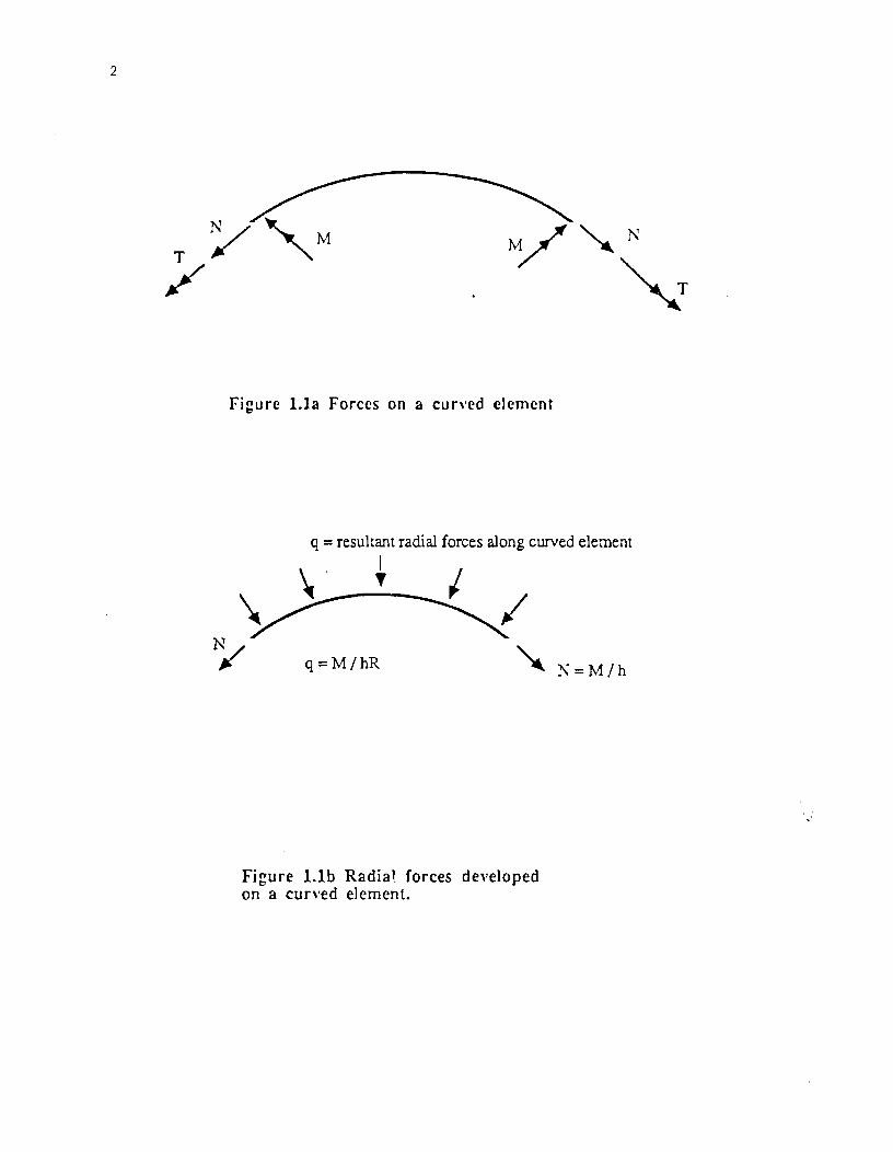
A single curved girder has forces acting on it which causes torsional loading on the girder as shown in
Figure 1.1a. Assuming that the flanges resist the full moment, the longitudinal force in the flange at any point
is equal to the vertical bending moment on a transverse section "M" in the girder at that point divided by the
centerline distance "h" between flanges. Because of the girder curvature, these axial forces are not collinear
along any given segment of the flange. Thus, to maintain equilibrium, radial forces must be developed along
the girder as shown in Figure LIb. The radial component of the flange force is directed outward when the
flange is in compression and inward when the flange is in tension. The radial forces are in opposite directions
as shown in Figure 1.2. It is the moment of these radial forces times the depth "h" which causes the twisting of
the girder about its longitudinal axis. Thus, the radial forces cause lateral bending of the girder flanges and
this results in the development of warping stresses.
1
2
Figure 1.1a Forces on a curved clement
q = resultant radial forces along curved element
\ . • I
q = M/hR
Figure 1.Ib Radia~ forces developed on a curved element.
N=M/h

3
In a curved girder, the bending and torsional moments are coupled; physically, this means that the
bending moments are influenced by the torsional moments along a girder and vice versa as shown in Figure
1.1a. A free body cross-section is shown in Figure 1.2. The horizontal forces are the previously described
radial forces. The in-plane and torsional moments vary along the girder length and since they are interrelated,
they cannot be solved directly. Unless the radius of curvature is sharp, the effect of the radial forces is much
higher than the effect of the torsional momenl
The addition of cross-frames to multi-girder systems greatly alter the physical behavior of the bridge.
A simple example of a two girder system is shown in Figure 1.3. and will help in the explanation. The
diaphragms introduce concentrated torsional moments which are a function of the diaphragm and girder
stiffness. In this simplified explanation, the diaphragms act as a concentrated reaction point for the radial
forces developed because of the curvature as shown in Figure 1.4. The approximate value would be "q" times
the length between diaphragms. Equal and opposite forces are thus developed at each cross-frame. To
maintain equilibrium of the cross-frame, vertical shear forces must be developed at each end of the cross
frame as a result of the cross-frame rigidity. These shear forces then react on the girders and either increase or
decrease the load on the girder as shown in Figure 1.5. The net effect of a braced, curved girder system is that
a portion of the load is generally shifted from the inner to the outer girders.
The V -Load method uses this simplification to analyze curved bridges. First the girders are
straightened out and the ordinary bending moments are determined at diaphragm locations. The second step
is to apply fictional V -Loads to each girder to account for the shift in load from the inner and outer girders.
It is useful to discuss in a general way the effect of certain bridge parameters on the behavior of a
curved bridge. As might be assumed, the shift of the load from the inner to outer girders increases as the
radius decreases. The shift of the load from the inner to outer girder decreases as the bridge becomes
torsionally stiffer. The things that increase the torsional stiffness of the bridge the most are the concrete slab,
the diaphragm spacing and the diaphragm configuration. The concrete slab is very stiff compared to the steel
framing and keeps the load transfer low. The main function of the diaphragm is to provide stiffness with a
closed section during construction. Thus, closer spacing and proper configuration of the braces is needed
during the erection stage. After the slab is placed, the diaphragms are still primary members but fewer are
needed since the slab stiffness is so large.
Perhaps the most critical time of a curved bridge is the construction phase. During the construction of
curved girders, the geometry and boundary conditions of the structure are changed at various stages of erection
changing from girder units with cross-frames to a complete bridge with a composite deck. Due to the geometry
of curved girders, they must generally be shipped in smaller lengths. This increases the amount of field
erection. Generally, the girders are erected in pairs and many times this involves cantilevering pieces. The
deflections and stresses at this stage must be determined since it may be the most critical time for the bridge.
After subsequent girders and diaphragms are added, the bridge becomes much stiffer and less critical. Once
the slab is provided, the behavior of the bridge is better since the slab provides a lot of stiffness. As a
designer, it would be useful to try different erection schemes to determine the best construction process. In
this way, the need for falsework or alternate erection schemes can be determined. What the designer actually
needs is an easy way to analyze the construction process as weU as the service life of the bridge.

4
H ....
H
Figure 1.2 Forces produced on :l single curved girder
d/2 dI2
H = MdJhR
h
Figure 1.3 Diaphragms for :l curved bridge
Y ~
M h
Figure 1.4 Diaphragm reaction on a curved flange

5
Girder 1 Girder 2
Figure 1.5a Diaphragm cross-section
~ H ~--..,...--
_ .... _- .04- H -4- -_ ..... _-
Figure 1.5b Additional loads due to girder curvature

6
1.1.2 Current Curved Girder Analysis Procedures
There are many different methods to analyze curved girders. Most of these methods involve the
computer since the analysis of even a simple curved girder by hand gets eXl1'emely complicated. In general,
these methods are categorized as follows:
1. Static Method - U.S. Steel (4)·
2. Computer Matrix Grid Method (8,9)
a) Three OOF
b) Five OOF
3. Space Frame Grid Method (8)
4. Finite Element Method (8)
5. Finite Difference Method (10,11,12,13)
• Number in parenthesis denotes items in References.
The first method is often called the "V -Load" method and generally follows the simplified explanation
for curved girder behavior in section 1.1.1. The V-load method allows for the direct determination of the
forces in the longitudinal girders and diaphragms by making certain assumptions relative to load or force
distribution. The V -load procedure is simple to use and is easily adapted to a personal computer for more
complicated cases. Recently, finite element analyses have been done to verifly the V-Load method for a
wider range of bridges. (4) Many practicing engineers use the V-Load method for approximate designs
because of its ease in use and then make fmal design checks with computer models.
The second method to be utilized consists of a computer oriented mattix method, which may consist
of three degrees of freedom or five degrees of freedom (3). The three DOF grid accounts for torsional effects,
but exclude warping. The five DOF gird , contains warping in the top and bottom flanges, thus increasing the
degrees of freedom by two.
The third method to be utilized is the space frame gird method with six OOF at each node (3). The
method models the girder flanges as beams and the webs as a series of cross and vertical elements. The
modeling of the girders in this manner include warping influences by summing the effects of axial loads and
vertical bending moments on the flanges.
The finite element method idealizes the bridge as a series of plate and beam elements with six DOF
at each node. Many times the preparation of the data and solution time can be excessive for large problems
even though the answers obtained are quite good.
The finite difference procedure permits direct solution of the differential curved girder equation. The
solution of the differential equations can also be solved by a rigorous closed-fonn technique or a Fourier series
method. Each of these three methods to solve the differential equation has its advantages and disadvantages
depending on the boundary conditions, number of girders and loadings. In all these methods, the solution of
the basic Vlasov (7) curved girder differential equations are utilized. Design aids and computer programs have
been developed for the finite difference method so that it is much easier to use.
The ideal analysis tool should be easy to use, accurate for a wide range of possibilities and be
relatively inexpensive to use. This research program was actually done in two separate parts by combining the
first and fourth methods.

7
1.2 OUTUNE OF PRESENT RESEARCH
1be research into the development of a curved girder analysis tool has been done in two parts. The
fIrst part developed a computer program for the V - Load method in which an approximate design could be
detennined The second part. which is the basis of this thesis, involved adapting an exitsting fmite element
program to analyze curved steel girder bridges.
1.2.1 Objectives and Purpose
The objective of this research was to develop an easy to use analysis tool for curved as well as
straight steel bridges. In addition, this research was to develop an easy to use analysis procedure of the
erection process. The philosophy behind this objective was to set certain limitations to balance the goals of an
easy to use program and one which is applicable to many bridge geometries.
The purpose of the research was to provide the designer with a new computer program design tool.
This new design tool will allow the structural design and analysis of curved girder bridges to be more effIcient
and accurate than presently possible. The benefit will be a reduction in engingeering time and prevention of
unforeseen construction problems.
1.2.2· Analysis Procedure
The main thrust of this research was to develop a pre-processor and a post-processor for existing fmite
element programs. The programs that were already developed were GENPUZ, PUZF83 and RECPUZ. The
programs utilize one and two dimensional fmite elements in a three-dimensional global assemblage with six
degrees of freedom (DOF) at each nodal point The two-dimensional elements have been used extensively
and have been reported in previous CFHR reports from projects 23 and 155.
The novel feature of the computer program developed in this project is that of substructuring. Using
the substructuring approach, bridge sections with identical properties that appear in sequence can be treated
very effectively since only the first section in the sequence has to be dealt with. The computer program
recognizes repeated substructures in both the stiffness calculations and the stress recovery. This, of course,
results in savings of both human and computer resources.
The goal of this project was to tailor simplifIed inputs to this concept of substructuring for curved steel
girder bridges. The individual substructure geometries and loadings are specifIed for the GENPUZ program.
GENPUZ is executed prior to PUZF83. GENPUZ prepares disk fIles containing element stiffnesses and node
numbers which are used in PUZF83. Infonnation on the global assemblage of the substructures as well as
boundary conditions are also specifIed for PUZF83. PUZF83 is a single level substructuring package which
computes nodal displacements. RECPUZ is done last and it is the stress recovery program. The program was
written in FORTRAN on the Cyber 750/170 of The University of Texas at Austin computational facilities. The
computer program was subsequently adapted to the SDHPf computer facilities.
13 OUTUNE OF CHAPI'ERS
Chapter 2 describes the background for the computer program and the documentation for the program.
Figures and small examples are also used to help the user understand the program quicker and easier.
Chapter 3 describes the output of the program. The user is given the background on the output and
help in discovering errors in data preparation.
Chapter 4 describes six example problems that demonstrate the ease and versatility of the program.

8
Chapter 5 describes the comparison of this program to other methods of analysis along with a
parameter study for different curved bridge geometries. The main purpose of this chapter is to demonstrate that
the program has been verified by other programs so that the user may be confident in the solutions obtained.
Also, the parameter investigation was used to study curved bridge behavior and to check both the fmite
element and V -load programs.
Chapter 6 presents conclusions and recommendations for other computer analysis programs.
CHAPTER 2. COMPUTER PROGRAM
21 GENERAL CONSIDERATIONS
The analysis of the bridge uses one- and two-dimensional finite elements in a three-dimensional grid. The
use of the program requires a respectable level of competence in finite element analysis on the part of the user. The
data genezator takes simplified input and creates ftnite element meshes, loads them and determines the deflection
and stresses. The user must decide how to best model the bridge so that these results are meaningful. Toward this
end, this chapter describes how the data generator takes the simplified input and models the bridge. The sections
that follow also discuss limitations and assumptions of the program with helpful suggestions on arranging the
input data.
2.2 BACKGROUND
To perform an analysis, the bridge must be divided into substructures. A substructure can be thought of as
a building block for a part of the structure. In this way, a wide variety of structural combinations are possible
through different arrangements of these blocks. An example of this concept of substructuring might clarify
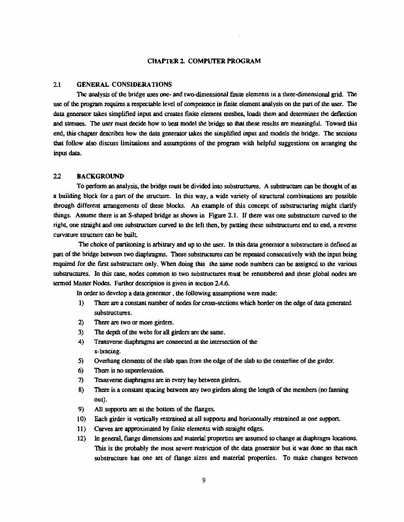
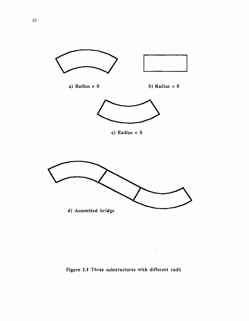
things. Assume there is an S-sbaped bridge as shown in Figure 2.1. If there was one substructure curved to the
right, one straight and one substructure curved to the left then, by putting these substructures end to end, a reverse
curvature structure can be buill
The choice of partitoning is arbitrary and up to the user. In this data generator a substructure is defmed as
part of the bridge between two diaphragms. These substructures can be repeated consecutively with the input being
required for the flfSt substructure only. When doing this the same node numbers can be assigned to the various
substrucbJres. In this case, nodes common to two substructures must be renumbered and these global nodes are
termed Master Nodes. Further description is given in section 2.4.6.
In order to develop a data generator, the following assumptions were made:
1) There are a constant number of nodes for cross-sections which border on the edge of data generated
substructures.
2) There are two or more girders.
3) The depth of the webs for all girders are the same.
4) Transverse diaphragms are connected at the intersection of the
x-bracing.
S) Overhang elements of the slab span from the edge of the slab to the centerline of the girder.
6) There is no superelevation.
7) Transverse diaphragms are in every bay between girders.
8) There is a constant spacing between any two girders along the length of the members (no fanning
out).
9) All supports are at the bottom of the flanges.
10) Each girder is vertically restrained at all supports and horizontally restrained at one support.
11) Curves are approximated by fmite elements with straight edges.
12) In general, flange dimensions and material properties are assumed to change at diaphragm locations.
This is the probably the most severe restriction of the data generator but it was done so that each
substructure has one set of flange sizes and material properties. To make changes between
9
10
a) Radius> 0 b) Radius = 0
c) Radius < 0
d) Assembled bridge
Figure 2.1 Three substructures with different radii

11
diaphragms, a substructure with diaphragms with zero physical properties can be added between the
actual diaphragms. Also, the diaphragm spacing can be altered so that it coincides with the change
in properties.
23 DATA GENERATOR
The bridge is modeled with one- and two-dimensional finite elements in a three-dimensional grid. A
typical partial model is shown in Figure 2.2. The concrete slab is modeled as a two-dimensional plate element and
is connected to the beam by rigid links. The rigid link is a beam element and goes from the center of the top flange
to the center of the conaete slab. The lOp flange is modeled as a beam element which is connected to the web and
the rigid link. The steel web spans between the top and bottom flange and is modeled as a plate element The
bottom flange is also modeled as a beam element and is connected to the web. The diaphragms are modeled as beam
elements and are connected to the top and bottom flanges. This modeling is common and results have been quite
good (6).
Two-dimensional plate elements are used for the concrete slab and the steel web. These plate elements can
be either quadrilateral or triangular elements. A typical quadrilatetal plate element is shown in Figure 2.3b. The
x-axis bisects side il andjk with the direction going from node i to node j. The y-axis is placed przpendicular to the
x-axis with the direction going from node j to node k. The z-axis completes a right hand coordinate system and
projects upward from the top of the element as shown in Figure 2.3b. A typical triangular plate element is shown
in Figure 2.3a. The x-axis is along line ij going from node i to node j. The y-axis and z-axis are then placed in a right
hand coordinate system with the z-axis pointing upward. The plate elements were originally developed as shell
elements with both membrane and bending stiffnesses. The plate elements have been used and described extensivly
in previous CFHR reports from projects 23 and 155. A constant thickness and orthotropic properties have been
assumed for the plate element. A plate element with orthotropic properties is especially convenient for the
concrete slab in the negative moment region and for the wet slab load in the dead load case since the elastic modulii
can be set to different values in the transverse and the longiwdinal directions.
One-dimensional beam elements are used for the diaphragms, flanges and rigid links. A typical beam
element is shown in Figure 2.3c. The x-axis goes from node i to node j. The y-axis is in the horizontal plane and the
z-axis is in the vertical plane for horizontal beams. These beam elements have axial, bending and torsional
stiffnesses. It may be assumed that the diaphragm is an axial element in a truss, in which case, the bending and the
torsional stiffnesses can be set equal to zero. The flange elements are assumed to be rectangular and the bending and
torsional stiffnesses are internally calclulated from the flange dimensions. The properties of the rigid link are
internally set in the program and have been set so that it would act as a shear stud and undergo little, if any,
deformations.
23.1 Nodal Coordinates
From the input for one substructure, the data generator determines the nodal coordinates, the element
node numbers and element properties required by the analysis program. As stated earlier, the substructure is
assumed to be bounded by diaphragms on each end. The data genezator numbers the nodes of the substructure from
left to right The local axis is placed on the left edge of the substructure at the same level as the bottom flange. If
the substructure is straight, the axis is placed at the midpoint between the first and last girder. If the substructure
is curved then cylindrical coordinates are used and the axis is located at a the point of origin of the reference line.

12
Quadrilateral Plate Elements
Flang/ Beam Elemen
"" Diaphragm Beam Elements
Figure 2.2 Substructure model
Quadrilateral Plate Elements

y
y
k
a) Triangular element
Nodes = 3 Ntri = 1
1
Nodes = 2
1 c) Beam element
k
i
b) Quadrilateral element
Nodes = 4 tIii = 4
Figure 2.3 Finite elements
13
j

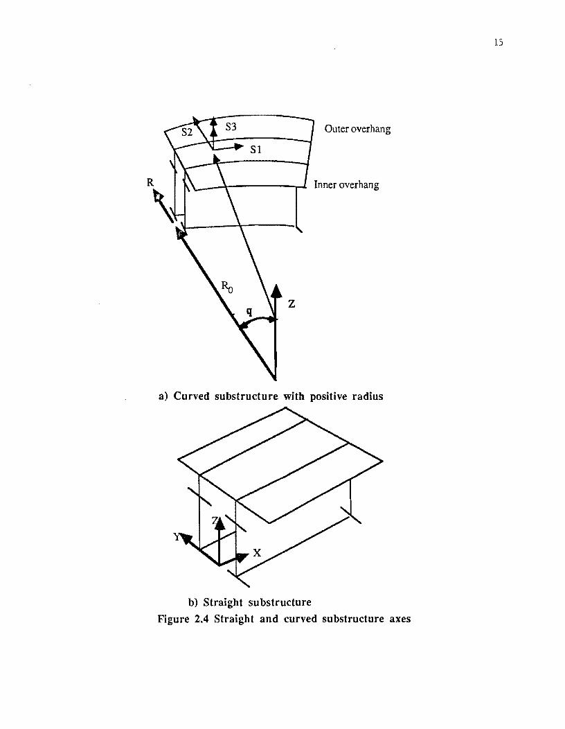
14
The locations of the axes are shown in Figures 2.4a and 2.4b. A positive radius of curvature is one in which the
substructure curves to the right and a negative radius of curvature is one in which the substructure curves to the
left As an example, the curvature shown in Figure 2.4a is positive.
An example of the node numbering process will help clarify things as shown in Figure 2.5. The data
genera1m' builds from left to right starting with the slab nodes. The outside overhang node is numbered fIrSt and is
placed at the mid-depth of the concrete slab. All the concrete slab nodes are place at the same vertical distance
equal to h2. The value h2 equals half the average bottom flange thickness plus the web depth plus the average top
flange thickness plus the soffit plus half the concrete thickness as shown in Figure 2.6a. The data generator then
moves down and determines the top flange nodes placed at a vertical distance hI. The value hi equals half the
average bottom flange thiclrness plus the web depth plus half the average top flange thickness as shown in Figure
26a. The bottom nodes are place at the mid-depth of the bottom flange. The average bottom flange and avenge
top flange thicknesses were input so that the vertical placement of the nodes is constant for the entire bridge. This
was a simplification that was done so that betu7 advantage could be taken of repeated substructures. When flanges
change dimensions, the vertical location of the node does not change but the new properties are centered on the node
as shown in Figure 2.6b. Also, the girder spacings do not change relative to each other but the girder spacings do
not h3ve to equal each other.
Three types of diaphragm bracings can be used with this data generator and they are the K-brace (Figure
2.7c), the X-brace with a top horizontal member (Figure 2.7a), and the X-brace without a top horizontal member
(Figure 2.7b). The node for the K-bracing is placed at hl(Fig. 2.7c) and at half of hi for the X-bracing as shown in
Figures 2.7a and 2.7b. A node was place at the intersection of the X-brace so that all brace configurations would
require the same number of nodes.
The next ttansverse row of nodes are placed at the location equal to the diaphragm spacing divided by the
number of divisions between diaphragms. An example of this is section B-B of Figure 2.5. The diaphragms are
added on the end and this is shown in section C-C of Figure 2.5.
23.2 Element Node Numbers
The element node numbers are determined after the nodal coordinates have been established as shown in
Fig. 2.7. The top nodes of the diaphragm on the left of the substructure between the first and second girders are
numbered first The exact numbering sequence is dependant on the type of diaphragm used as shown in Figure 2.7.
After the diaphragms are numbered, the nodes for a rigid link between the top flange and the concrete slab are
determined. The slab element is numbered counter-clockwise as viewed from above starting with node two. In this
way, the local x-axis and y-axis are generally in the same direction as the global axis. The slab elements are then
numbered next from left to right After the slab, the top flanges of the girders are numbered from left to right
The node numbers for the web elements are determined next with node i equal to the first bottom flange node. The
nodes of the bottom flanges are then numbered from left to right The process is repeated for each division between
the diaphragms. The diaphragms are only added at the end of each substructure. The element node numbers fm the
bottom horizontal bracing are determined last and the bottom brace sequence is in the same order which they were
input The physical properties of the elements are determined at the same time as the node numbers.
15
Outer overhang
Inner overhang
z
a) Curved substructure with positive radius
b) Straight substructure
Figure 2.4 Straight and curved substructure axes

16
20 21 22 23 24 C C
I ,~ I 'Spacing of
12 13 :14 15 B B 11 Diaphragms
,~ (Sdia) Sdia/2
AU= 4~A 'r "
2 3
Plan View Reference line
1 2 3 4 5
6 7 -------,.--
h2
Reference line Dgir2
Section A·A
11 12 13 14 15 20 21 22 23 24
16 17 25 26
18 19 27 28
Section B·B Section C • C
Figure 2.5 Element node numbering.

Te
(Average top fhmge thickness)
Tftavg
Girdwd
(Web depth)
(Average bottom flange thickness)
Tfbavg T Figure 2.6a Node location.
"" ft A "" • .... ... A"""AAA'"
A A A ...... A .. "., .. ...
.... A "" " A ... "'" <lit. A
Te/2 + Soff + Tftavg!2
hI = Tfbavg12 + Girdwd + Tftavg12
" ....... A " A A ... A A
~ ....... .
f-~-~-~-~--~-~-~-~-~-~-~-~-~-~~--~-~-~-~-~-~-~-~-~-~-~-~-~- --r
h2
hI h2
Figure 2.6b Model with change in flange dimension.
17

18
a ) X- brace with top horizontal brace Ibrace = 1
6~ ~tv d) Rigid links
11
k J
CD 1 i
1
6 1
12
k
1
2
® 1
8
g) \Yeb
b ) X- brace without top horizontal brace Ibrace = 2
j 16 17
2
1 6 7 i
f) Top flanges
13 14
J k J k
® ® 1 1 i I
3 4
e) Slab
16 7 k 1
8
® j
18 9 i
Figure 2.7 Element nodes
j
1
b)
9 c) K - brace
Ibrace = 3
18 19 j
1
8 9 i
Bottom flanges
15
J
® i
5
17 k
i 19

19
233 Automatic Mesb Size The program has the capability to detennine a fll'St approximation for the refmement of the mesh. The
coarseness of the mesh is done with the idea to keep the elements as square as possible. Since the web only has one
plate element in the vertical direction, the program sets the size of the rest of the plate elements as close as
possible to the web depth. This routine should be used with a cautious eye since the coarseness of the mesh is only
done once for the bridge. If the diaphragm spacings change much then the size of the mesh may not be the most
economical and worse yet the answers may not be reliable. The aspect ratio of the quadrilateral plate elements are
given so that any problems can be detected.
23.4 Loads All loads are placed as equivalent concentrated loads at the nodes. Dead loads due to surface loads on the
concrete slab are superimposed on the concrete slab elements as an increase in density. Edge loads on the overhang
are smeared over the overhang eJements as an increase in density of the overhang elements. Live loads due to bUck
loading or lane loading are also superimposed on the nodes of the concrete slab elements. In addition, it is possible
to add more loads from input data by hand onto the bridge. This would represent loadings not covered by the data
generator such as wind loads and braking loads.
235 Changing Substructure Values A new substructure needs to be defmed if there is any difference between the previous substructure. For
example, a new substructure is needed if the flange dimensions change. The only additional input required are the
values that change from the previous subsbUCture. When this update is done, the number of repeated substructures
of this same type must always be included. The data generator then generates the substructure again. Also,
changing loads between substructures do not require a new substructure.
23.6 Custom Substructures If a part of the geometry of the bridge does not Jend itself to the data generator routine then the user must
input that substructure by hand. This input follows the documentation for section 2.4.6. Mter all the data are
included, then this custom substructure can be placed as the next subsbUcture in the bridge. The bridge can thus
contain a mixture of custom and data-generated substructures.
23.7 Master Nodes The arrangement of the substructures to fonn the entire bridge is done with master nodes. These master
nodes are at the intersection of all substructures and at each end of the bridge. In a simplified sense, the master
nodes are the global numbering of all the diaphragms. The local nodes of each substructure must be renumbered to
match these master nodes. The data generator does all of this automatically but the user must understand the
concept of master nodes in order to interpret the output
23.8 Boundary Conditions The boundary conditions may be imposed on either the master nodes or the internal nodes of a
substructure. In most cases, master nodes are used because the boundary conditions are imposed at diaphragm
locations. When the support is between diaphragms, then the boundary conditions must correspond to the local
nodes for that substructure. The most common occurrence would be if the support is skewed.

20
The data generator has the capability to handle two kinds of substructures which have skewed suppons.
The distinction is made between a slight and a severe skew. A slight skew is one in which the mesh is slightly
distorted to accomodate the support skew as shown in Figures 2.8 and 2.18. The suppons can be at the diaphragms
in which case the diaphragms follow the support line and the master nodes are used. The support can be placed
between the diaphragms in which case local nodes are used. Usually diaphragms are required at support locations but this modeling allows radial supports when the support is only slightly skewed. The slight skew substructrue
(IROUTE=3) is most versatile in that it can be used at both end and interior locations as shown in Figure 2.8b with
litttle additional inpUL Also, the skewed substructure can be used without support conditions which may be
useful next to skewed supports.
A severe skew is one in which the diaphragms intersect at the point where the girders are supported as shown in Figure 2.8c. 1be diaphragms still bound a single substructure but the suppons can span one or more
substructures as shown in Figure 2.19. Because of the difficulty in creating a general data gent'J'ator for a severely
skewed end support, the severely skewed substructure (IROUlE =4) only applies to interior suppons. If the
support conditions do not correspond to these categories then the boundary conditions must be input by hand. See
the respective sections for further clarification.
1be data generator allows the user to specifiy many things pertaining to the support conditions. All
supports are vertically restrained but the user can specify which support is horizontally restrained. In addition,
the user can input vertical support spring stiffnesses or intitial vertical displacements for any and all supports.
This is especially useful if different elastomeric pads are used or a support undergoes settiemenL
23.9 Summing Load Cases
1be program has the capability to sum stresses for different load cases. In this way, it is convenient to run
the dead load case and then run the live load for the worst case loading. The stresses for the dead load and live load
can then be summed up with the stresses for the latest run printed out alongside the total stresses.
2.3.10 Erection Stages
The erection procedure can be approximated by making separate computer runs for each stage. Each
erection stage is input with the girders and the length to be erected. The program then uses the density and the
elastic modulus to model the bridge with the stiffness of alJ the previous stages but only the load of the last
stage. Superposition is then valid to sum up the stresses for the erection procedure in the same way different load
cases are summed.
2.3.11 Substructure Types
Th€2'e are thus five possible types of substructures which can be used in this program. They are: 1) An initial mesh-generated substructure in which all the data to generate the mesh is inpUL When
substructure 3 or 4 is the first data generated substructure then all the data for the bridge also needs
to be inpUL
2) An update of some previously specified value of a mesh-generated substructure.
3) A substructure with a slightly skewed mesh. This substructure mayor may not have supports. If it
has supports then the supports are possible either at diaphragm locations or at the interior of the
substructure.

1
1
Iroute = 5 ,
,
1
Figure
2 3 4 5
2 \ 4 5 , ~
\
Iroute = 4 , 2 "'~ ..... -..... 4 5
-, \
2 3 4 5
\
6
a) Radial supports Span 1 = 3 Substructures Span 2 = 2 Substructures
b) Slight skew of 3 supports.
,
Span 1 = 3 Su bstructures Span 2 = 2 Substructrues Substructures 1,3 and 5 are generated with Iroute = 3.
c) Severe skew of supports. Span 1 = 4 subst. Span 2 = 3 subst.
Iroute = 5 ,
d) Strange interior skew. Span 1 = 5 substructures Su bstructure 3 must be input with Iroute = S.
2.8 Number of substructure per span.
21

22
4) A substructure with the ability to handle severely skewed supports. This substructure may have
supports at both diaphragm and interior node locations but it is only good for interior supports of
the txidge.
5) A custom substructure that does not lend itself to any of the data generated substructures.
2.4 INPUT DOCUMENTATION
This section describes the input required for GENPUZ, PUZF83 AND RECPUZ. These programs
combine to form KURV87. The variable corresponding to the five types of subsbUctures is called IROlITE. The
documentation will show how to prepare the data files for all of these types of substructures. Further
explanations are found in sections 2.5, 2.6 and 2.7. Appendix C includes the input in tabular form for easy
reference. The labels in paranthesis are the same ones used in the program and help clarify explanations in other
parts of this documentaion. In the description of the input data the following abbreviations apply:
A = Alphanumeric
F = Floating point number (must be typed with a decimal point).
I = Integer value (must be packed to the right of the field).
2.4.1 Initial Data for Program
A) CONTROL CARDS
LINE COLS. TYPE
1
2
3
1-~
1-~
1- 5 6-10
A
A
I
I
11- 15 I
16- 20 I
21- 25 I
Labeling information for this computer run.
Labeling information for this computer run.
Number of different types of substructures. 196 Maximum (Nogp)
Plotting option. (Ipl)
= 1 , to execute plots in XY and yz plane for each substructure.
= 2 ,to also execute plots of concrete slab stresses by nodes.
Output print option. (Idef)
= 0 , for minimum output display. This outputs only stresses and the
minimum echoing of input data.
= 1 , for additional output display. This outputs deflections by master nodes
and more echoing of check prints.
= 2 , for maximum output display. This outputs deflections by both element
and master node with more check prints. For large problems, there can be a
lot of elements and this output will be quite voluminous.
Load case of this computer run. Also used as erection stage. (Jrec)
Number of steel erection stages to be inpUL (lrec) This number will be
different than the current erection stage if concrete stages are to be
superimposed on the steel stages.

23
LINE COLS. TYPE
26 - 30 I Summation of stresses with previous load case. (lrcsum)
= 0 , no stress summation.
31- 35 I
36-40 I
41-45 I
= 1 , if the stresses of this run are to be added to the last run which Ircswn
equaled one. This is used to add dead load to live load and for summation of
erection stage stresses.
Number of prescribed support displacements or spring constants to be input
(Nospg) Suppon settlements and springsapply to the vertical direction only.
Automatic mesh size determination. (Kgen)
= 0 , number of mesh divisions to be input by user.
= 1 ,program internally generates size of mesh.
Composite or noncomposite girder. (Koolp) This choice makes the rigid link
a truss element and sets all concrete slab stresses equal to zero.
= 0 , Girder is composite.
= 1 ,Girder is noncomposite.
B) SUPPORTCONDnnONS
The support conditions are specified by the number of spans and the number of substructures per
span. For further information see Section 2.5.2 and Figure 2.8.
LINE COLS. TYPE
1 1- 5 6-10
I
I
11- 15 I
16- 20 I
Number of spans. 10 maximum (Nspan)
Number of substtuctures until the suppon is pinned. (Nfix)
= 0 , if bottom of girders at the first diaphragm are pinned.
>= 0 , if bottom of girders at the first diaphragm are on rollers.
<= 0 , if bottom of girders at the fU'St diaphragm are not supponed.
Number of substructures for flfSt span. (Nsubbc) For substtuctures with
skewed supports, count the number of substructures in a span until the next
substructure is not supponed. An example is shown in Figure 2.8.
Number of substtuctures for the second span. Input the number of
substtuctures for each span in "15" format until all spans are input
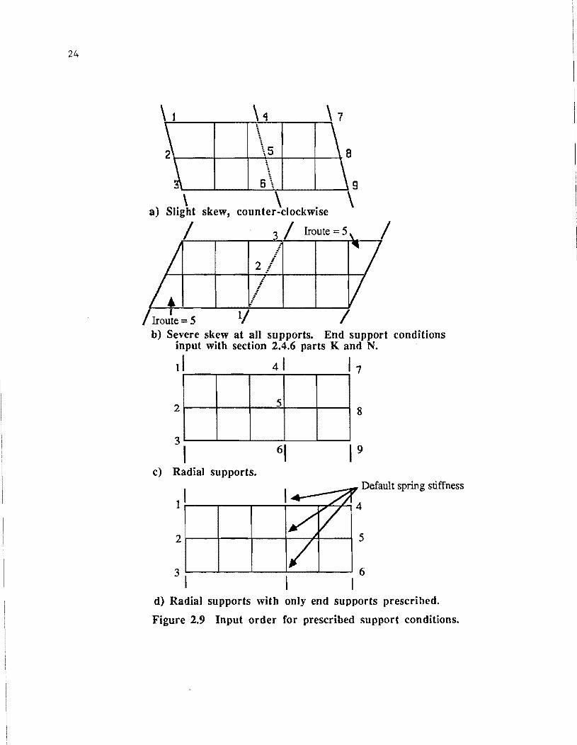
C) PRESCRIBED SUPPORT CONDnnONS
The number of lines for input should equal the number of suppon displacements or
spring stiffnesses specified in the control cards (Nospg). The suppon restraints
must be input in the order that they are encountered when numbered from left to
righL Thus, they shall be input in increasing order relating to the master nodes.
When the support is in the interior of a substtucture then the input should follow all
the input to the left of the interior support. A couple of examples of the proper order of
input are shown in Figure 2.9. Also, if one girder at a suppon has the input for
reslnlints then all the girders at that suppon must have boundary conditions input
24
skew, \ .
counter-clockwise
2/ I
: :
:
/ Iroute = 5 1/ b) Severe skew at a1l supports. End support conditions
input with section 2.4.6 parts K and N.
11 41 I 7
5 2r----+---+--=f----+---IS
3~--~--~--~--~--~
1 61 1 9 c) Radial supports.
Default spring stiffness
11~~---~---~---~~~~~
21----I----I-----1---.A-------I5
3 ~-~-~----~--~-~ 6 I I
d) Radial supports with only end supports prescribed.
Figure 2.9 Input order for prescribed support conditions.

25
LINE COLS. TYPE
1
LINE
1
1- 5 I
6-10 I
11-20 F
Numbc7 of subsbUCtureS until a support. (Jspg) This number should correspond to the
total number of substructures going from left to right.
Displacement or spring index. (Kspg)
= 2 , for input corresponding to a prescribed displacement.
= 3 , for input corresponding to a spring stiffness.
Displacement or spring value. (V spg)
= dispJacement specified. Positive upward. - inches -... = sping stiffness specified. - kips / inch -
D) ERECTION PROCEDURE (one line for each stage)
COLS.
1 -10
11-20
21- 30
31-40
TYPE
F
F
F
F
Starting girder for erection stage. (Kgrst)
Ending girder for erection stage. (Kgren)
Starting substructure for erection stage.(Ksbst)
Ending substructure for erection stage. (Ksben)
IT just the diaphragms are added between two girders then the first two entties must be
input as the negative of the girder numbers. The starting subsbUCture must start with
zero at the beginning of a bridge. If only one substructure is added, then the last two
entties must be the same value. See the example of a four-girder bridge as shown in
Figure 2.10.
2.4.2 IROUTE = 1
This choice generates the first data-generated subsbUCture based upon the initial bridge data. This choice
should be done only once. Subsequent changes should be done with IROUIE = 2 so that values that do not change
from one substructure to the next do not have to be input again. If the intiaJ mesh is for a skewed support. i.e.,
IROUIE = 3, or = 4, then this input must come rust and the input required for either IROUIE = 3 or IROUIE = 4
should immediately follow.
A) SUBSTRUCTURE INDEX
LINE COLS. lYPE
1 1-5 I = 1 , Type of substructure. (Iroute)
B)BREDGEGEOMETRY
LINE COLS. lYPE
1 1- 5
6-10
I Number of times this same subsbUCture is repeated consecutively. 16 Maximum. (Nv)
I Number of mesh divisions between girders. 10 Maximum. (ldivt)

26
Substructure No. 1 2 3 4 8 9 5 6 7
---- ... ----. 10\
1 , , , . , , , , 2 , , , , , , , , , , , I , , , , , , , , , , , , , , , , , , , '- - - - 04 - - - - I-
, ---- .. ----'---- - - - - + - - - - '- - - - -' , , I --- -,- --- I , ' , I
I , , I I I , , , , I I , , , , I , I , , , ,
L ____ ~ ___ J ____ ~ ____ - - - -' - - - - .& - - - -
____ , ____ oJ ____ , 4
3
a) Stage one It
Girder No.
, , , ,
Stage no. Starting Sub. Ending Sub. Starting Girder Ending Girder 10812
1 2 10 \ 1 3 4 5 6 7 8 9 ----,- ----. , , , , , I
, I , I , , I
, , , I , I , , , , I
, I , , , , , , I , I I , I ----04----'
I , I , I , I ,
---------
b) Stage two
Stage no.
1
Starting Sub. Ending Sub. Starting Girder Ending Girder
o 8 1 2 2 o 8 3 4
Figure 2.10a,b Erection stage example
2
3
4

---- .. ----.
Substructure No. 1 2 3 4 5 9 10\
1 6 7 8
I I I I I I 1 1 2 1 1 1 I 1 1
- - - - 1- ____ I 3 1 1 1 1 1 1 I 1 ----.1 ____ 1 4
c) Stage three It
Girder No.
Stage no. 1
Starting Sub. Ending Sub. Starting Girder Ending Girder o 8 1 2
2 o 8 3 4 3 o 8 -2 -3
1 2 3 4 5 6 7 8 9
d) Stage four
101
Stage no. 1
Starting Sub. o
Ending Sub. Starting Girder Ending Girder 8 1 2
2 o 8 3 4 3 o 8 -2 -3 4 9 10 1 4
Figure 2.10c,d Erection stage example
1
2
3
4
27

28
LINE COLS. TYPE
2
11- 15 I Number of mesh divisions between diaphragms. 10 Maximum. (ldivl)
ldivt and ldivl are not needed if mesh size is automatically determined.
16 - 20 I Number of girders. 10 maximum. (Ngir)
1-10 F Reference radius of bridge. -feet- See Fig. 2.4b. (Rref)
= 0, For a straight substructure.
>= 0, For a substructure that curves right
<= 0, For a substructure that curves left
11 - 20 F Thickness of concrete slab. -in- (Tc)
21- 30 F Inside overhang of concrete slab. -ft- (Ovin)
31 - 40 F Outside overhang of concrete slab. -ft- (OvOUl)
41 - 50 F Reference line spacing of diaphragms. Reference line arc length between diaphragms for
curved substructures. -ft- (Sdia)
C) GIRDER INFORMA nON
LINE COLS. TYPE
1 1 - 10 F Distance from reference line to girders. (Rgir) Input all distances of girders in ascending
71-80 F
2 1-10 F
11-20 F
21-30 F
31-40 F
41-50 F
3 1-10 F
11-20 F
21-30 F
31-40 F
order of girder numbers in "FlO" field length. Use more than one line if required. -ft-
" "
Distance from reference line to girder.
Web depth. -in- (Girdwd)
Not including flange thicknesses.
Web thickness. -in- (Tw)
Average top flange thickness for entire structure. -in- (Tftavg)
Average bottom flange thickenss for entire structure. - in- (Tfbavg)
Distance from top of the flange to bottom of the concrete slab. Assumed constant -in
(Soff)
Input the following for each girder.
Thickness of top flange. -in- (Tft)
Width of top flange. -in- (Bft)
Thickness of bottom flange. -in- (Tfb)
Width of bottom flange. -in- (Bfb)
D) DIAPHRAGM INFORMA nON
LINE COLS. TYPE
1 1 - 5 I Diaphragm bracing configuration for beginning of substructure. (lbrace(I»
= I, For X-bracing with top horizontal member.

LINE COLS. TYPE
2
6 -10
11-15
16-20
1- 10
11-20
21-30
31-40 41-45
I
I
I
F
F F
F
I
46-50 I
51- 55 I
56-60 I
61- 65 I
66-70 I
= 2, For X-bracing without top horizontal member.
= 3, Fey K-~ing.
Diaphragm bracing configuration for end of substructure. As above. (Ibrace(2) )
Number of different types of diaphragm bracing members. (Ndifbr)
Number of bottom horizontal braces. (Ibrbot)
All assumed to have the same properties.
Half the area of the diagonal diaphragm brace -in2- (Adia)
Half the moment of inertia for the 1nce about the horizontal axis. -in4- (Diy)
Half the moment of ioeJtia for the brace about the vertical axis. -in4- (Diz)
Half the torsional moment of ineztia. -i04- (I'orj)
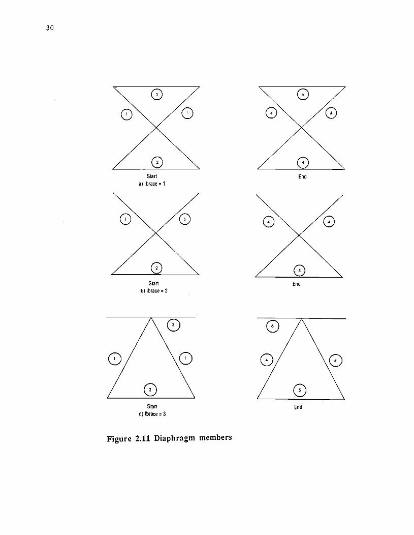
Description index for locating the properties of the diaphragms. (Thr) See Figure 2.11
for further information.
The number corresponds to the foUowing description:
= I, For diagonal member of beginning brace. = 2, For bottom member of beginning brace.
= 3, Fey lOp member of beginning brace.
= 4, For diagonal member of ending brace.
= 5, Fey bouom member of ending brace.
= 6, For top member of ending brace.
Description index for second brace member
Description index for third brace member
Description index for fourth brace member Description index for fifth brace member
Description index for sixth brace member.
29
E) BOTIOM HORIZONTAL LAlERAL BRACING INFORMA nON
LINE COLS. TYPE 1- 10 F
11-20 F
21-30 F
31-40 F
2 1- 5 I
6-10 I
Full area of diaphragm for bouom horizontal bracing. -in2- (Adia(7»
Full moment of inertia for bouom horizontal bracing about the horizontal axis. -in4-
(Diy(7»
Full moment of inertia for bottom horizontal bracing about the vertical axis. -in4-(Diz(7»
FuU torsional moment of inertia for bouom horizontal bracing. -in4- (I'orj(7»
Girder number in which the brace starts. (Ngsbot)
Girder number in which the brace ends. (Ngebot)
This must be input for each bouom brace. The start of the substructure is the cross
section in which the node numbering begins. See Figure 2.12 for further information.
30
o
Start End a) Ibrace = 1
Start End b) Ibrace = 2
Start End c) Ibrace = 3
Figure 2.11 Diaphragm members

31
Girder 1 Girder 2
Girder 1 Girder 2
Figure 2.12 Horizontal lateral bracing

32
F) MATERIAL PROPERTIES
LINE COLS. TYPE
1
2
1-10 F
11-20 F
21-30 F
31-40 F
1-10 F
11-20 F 21-30 F
Modulus of elasticity for concrete in the x-axis direction. -ksi- (Ec(1»
Modulus of elasticity for concrete in the y-axis direction. -ksi- (Ec(2»
Poisson's ratio for concrete for a stress in the x-axis direction. (poise)
Denstity of concrete. -kcf- (Dense)
Modulus of elasticity for steel Assumed the same in both directions
-ksi- (Est)
Poissons's ratio for steel. (poisst)
Density of steel. -kef- (Densst)
G) SLAB LOAD INFORMATION
LINE COLS. TYPE
1 1-10 F
11-20 F 21-30 F
31-40 F
Negative is downward.
Curb load of outside overhang. -k I ft- (Curbld(l»
Curb load of inside overhang. -k I ft- (Curbld(2»
Superimposed surface load on concrete slab. -ksf- (Surfld)
Live load index. (Zlivld)
= 0.0, For no live load.
= 1.0, For truck loading.
= 2.0, For lane loading.
H) mUCK LOAD INFORMATION
See Figures 2.13 and 2.14 for further description.
LINE COLS. TYPE
1
2
1-5
1-8 9-10
I Number of Trucks. (Ntruck)
A Truck name.
I Repetition index. (Ibid) This value is used if the truck input directly preceding this one
is the exact same.
= 0, If Ibis is a new uuck geometry.
11-20 F = I, If the geometry of this truck was input immediately preceding this uuck.
Load impact factor. (Dlf)
21- 30 F
31-40 F
Longitudinal location of centroid of truck from the reference line of the bridge. -ft(Xpos)
Transverse location of centroid of truck from the reference line of the bridge. -ft(Ypos)

locolAxis -~ 41'- ~ t .. + ~ ~ ~
• Global longitudinal coordinate I Globaltronsvel'$e coordinate lLe. the longitudinal distance li.e. the tronsveue di'llance of the centroid of the lane lood of the centroid of the lane from the reference line.} load from the reference line.,
Beginning of Bridge
a) Truck placement on a straight bridge.
Global long. co-ord (arc length)
--Reference radius
b) Truck placement on a curved bridge
Figure 2.13 Global truck positioning
Transverse distance from reference line to centroid
33

34
I~ -14 ' 14 ' 1
c::::::=:) c::::::=:)
i~:. 16k 16k 4k
-t-c::::::=:) c=::J c::::=>
16k 16k 4k
a) Truck example Load Local transverse Local longitudinal
(lcips) location (ft) lcx:ation (ft)
4 3.0 14.0 4 - 3.0 14.0 16 3.0 0.0 16 -3.0 0.0 16 3.0 -14.0 16 -3.0 -14.0
I: plk
pxlk ~ 1
Area 4 Area 3
xl pI = P x Area31 Areatot p2 = P x Area41 Areatot p3 = P x Area 11 Areatot p4 = P x Area21 Areatot
Area 1 pxlk = pxl x plk l(pxl +px2)
i pxij = pxl x pij l(px 1 +px2) I: prij ~ ~ pij
b) Wheel load allocation to nodes
Figure 2.14 Truck loads

LINE COLS. TYPE
41-50 F
52-55 A
3 1-5 I
4 1-10 F
11-20 F
21- 30 F
35
Radius of curve to the reference line of the bridge at the position of the centroid of the
truck. -ft- (Radtr)
Direction of truck. (Idir)
= Forw, For a truck going from left to right
= Back, For a truck going from right to lefL
The next lines are needed if Ibid = O. Positive is downward.
Number of wheels. (Nwheel)
Wheel load. -kips- (Tdd)
Local transverse location of wheel. -ft- (Centtt)
Local longitudinal location of wheel. -ft- (Centlg)
I) LANE LOAD INFORMA nON
LINE COLS. TYPE
1 1- 5 I
2 1- 8 A
11-20 F
21-30 F
31-40 F
41-50 F
3 1-5 I
6-15 F
4 1-10 F
11-20 F
21- 30 F
5 1-10 F
11-20 F
21- 30 F
31-40 F
Number of lane loads. 10 Maximum. (Nlanld)
Name of lane load.
Load impact factor. (Dlf)
Longitudinal distance of the centroid of the lane load from the reference line of the
bridge. (Xpos) -ft-
Transverse distance of the centroid of the lane load from the reference line of the bridge.
(Ypos) -ft-
Radius of cmve to the reference line of bridge during length of lane load. (RadIn) -ft
If the curvature of the bridge changes in the lane load then two lane loads must be input
corresponding to the respective radii.
Number of concentrated loads. (Nconld)
Uniform lane load. This should be the same for all lane loads. Positive up -ksf- (Wdist)
Concentrated load. Negative down. (Tdd) -kips
Local transverse location of load. (Centtt) - feet
Local longitudinal location of load. (Centlg) -feet-
Transverse location of upper left comer of the lane load. -ft
Longitudinal location of upper left comer of the lane load. -ft
Transverse location of lower right comer of the lane load. -ft
Longitudinal location of lower right comer of the lane load. -ft-

36
LocolAxis _
~ I + J I
- -I f
Globallongiludinal co-ordinole I Globoltronsverse co-ordinole (i.e. the longitudinol dislance fl.e. the transverse dislonce of the centroid of the lone load of the centroid of the lone From the reference line.] load from the reference line.'
8eginning of Bridge
a) Lane load placement on a straight bridge.
Global long. co-ord (arc length)
Reference radius
Transverse distance from reference line to centroid
b} Lane load placement on a curved bridge.
Figure 2.15 Global lane load positioning
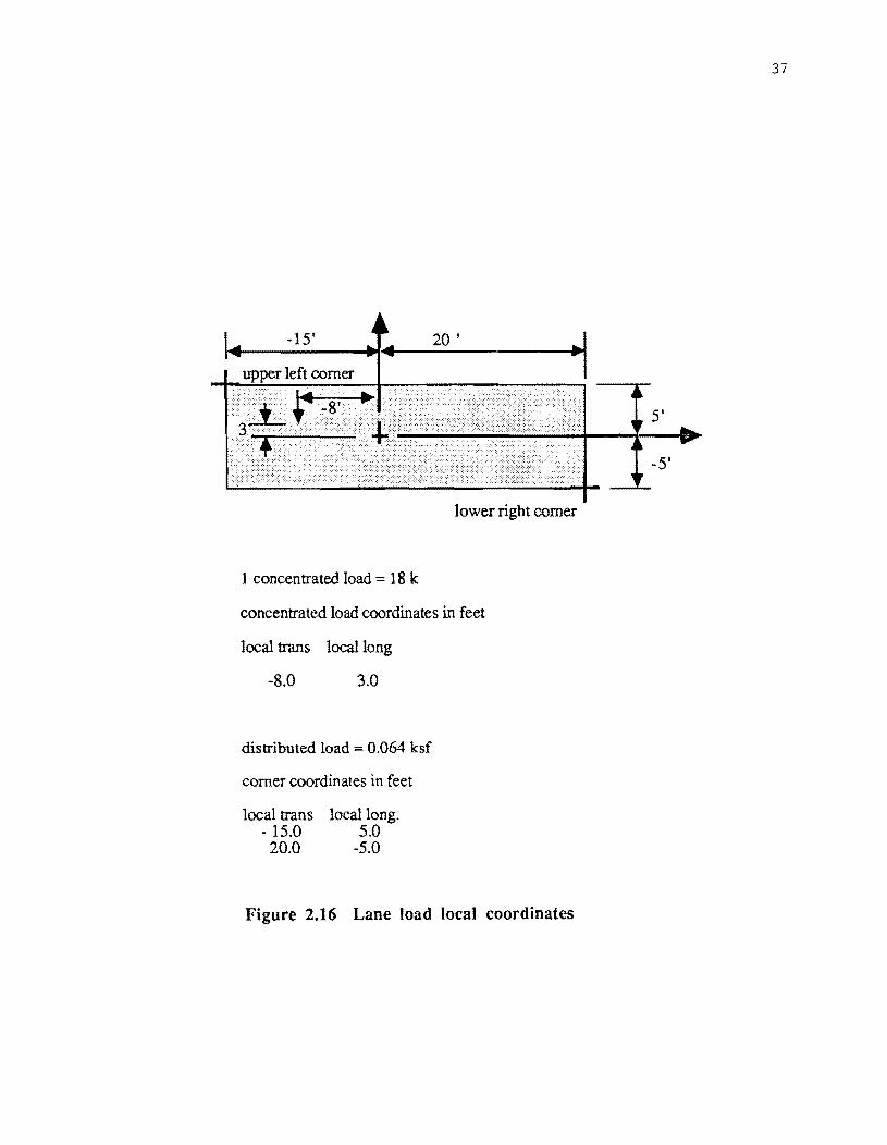
37
lower right comer
1 concentrated load = 18 k
concentrated load coordinates in feet
local trans local long
-8.0 3.0
distributed load = 0.064 ksf
corner coordinates in feet
local trans local long. - 15.0 5.0 20.0 -5.0
Figure 2.16 Lane load local coordinates

38
1) ADDmONAL LOADS
LINE COLS. TYPE
1 1-5 I
6-10 I
11- 15 I
21- 30 F
31-40 F
41- 50 F
51-60 F
2.43 IROurE = 2
Loads are input by elements. Each line of data is superimposed on loads that may exist
for that member. End this section by placing a zero in column one. Signs of additional
loads should follow element axis as shown in Fig. 2.3a, band c.
DOF of forces for this element (i.e., 1 - 6) (Idof)
Substructure where this element is located. (Jsubld)
Element number. (Kelno)
Force at node I of this elemenL (P(1»
Force at node J of this elemenl (P(2»
Force at node K of this elemenl (P(3»
Force at node L of this element (P(4»
This option is used to update a previously specified parameter. The parameters that can be changed are
shown in the following lisl Each parameter is assigned a number (Nalt). To change the value of a parameter,
simply specify the parameter to be changed and the conesponding new value.
A) SUBSTRUCfURE INDEX
LINE COLS. TYPE
1 1- 5 I = 2 , Type of substructure. (Iroute)
B) NUMBER OF VALUES TO BE CHANGED
LINE COLS. TYPE
1 1- 5 I Number of values to be changed. (Noval)
C) UPDATE OF VALUES
LINE COLS. TYPE
1 1 - 5 I Parameter number specifying the parameter to be changed. (Nalt)
6-15 F New value of parameter. (Value) Input the number as the same type as input for
IROUTE = 1. i.e. integer or real.
Nalt = 1, Number of repeated substructures. (Nv)
= 2. Number of divisions along the girdez. (Idivl)
= 3. Radius of reference line of bridge. -Ct- (Rref)
= 4 • Spacing of diaphragms. -Ct- (Sdia)
= 5. Thickness of the web. -in- (Girdwd)
= 6. Diaphragm bracing configuration and properties.

39
Additional input is required and the second space in line two should be left blank.
The following input is required for new diaphragms.
LINE COLS. TYPE
1
1
LINE
1
1 - 5 I
6-10 I
11-15 I
Diaphragm bracing configuration for the beginning of the SUbSbUCbJre.
(Ibrace(1) )
= I, For X-bracing with top horizontal member.
= 2, For X-bracing without top horizontal member.
= 3, Foc K-Incing.
Diaphragm bracing configuration for end of SUbsbUCture. As above. (lbrace(2) )
Numbez of different types of diaphragm bracing members. (Ndifbr)
The following should be input for each different brace. 1-10 F Half the area of the diaphragm. -in2- (Adia)
11-20 F
21-30 F
31-40 F 41-45 I
Half the moment of inertia for the brace about the horizontal axis. -in4- (Diy)
Half the moment of inertia for the brace about thevertical axis. -in4- (Diz)
Half the torsional moment of inertia. -i04- (forj)
Description index for locating the properties of the diaphragms. (lbr)
The numbez corresponds to the following description:
= I, For diagonal member of beginning brace.
= 2, For bottom member of beginning brace.
= 3, Foc top membez of beginning brace.
= 4, For diagonal member of ending brace.
= 5, Foc bouom membez of ending brace.
= 6, For lop member of ending brace.
46-50 I Description index for second brace member
51-55 I Description index for third brace member
56-60 I Description index for fourth brace membez
61-65 I Description index for mth brace member
66-70 I Description index for sixth brace membez.
Nalt = 7 ,Bouom horizontal bracing. New values for the dimensions of the braces should be
input as the following:
COLS. TYPE
1- 10 F Full area of diaphragm for bottom horizontal bracing. -in2- (Adia)
11-20 F Full moment of inertia for bottom horizontal bracing about the horizontal axis. -in4-(Diy)
21-30 F Full moment of inertia for bottom horizontal bracing about the vertical axis. -in4-(Diz)

40
LINE COiS. TYPE
1
1
31-40 F Full torsional moment of inenia for bouom horizontal bracing. (TOIj)
1- 5 6-10
1-10
11-20
21-30
31·40
Nalt = 8 • Number of bottom braces in a aoss-section. This number can be input as zero and
no bouom bmces will be added.
I
I
= 9 • Bottom bracing geomeuy. The following lines must be input for each boUDm
brace. The second value in d1is row sbou1d be zero.
Girder number in which the brace starts. (Ngsbot)
Girder number in which the brace ends. (Ngebot)
This must be input for each bouom brace. The start of the substructure is the cross
section where the node numbering begins.
Nalt = 10. Flange dimensions. The following must be input for each girder. The second
value in this row should be zero.
F Thickness of top flange. ·in- (Tft)
F Width of top flange. -in- (Bft)
F Thickness ofbouom flange. -in- (rfb)
F Width of bouom flange. -in- (Bfb)
Nail = 11. Modulus of elasticity of concrete in the x-axis direction.
-ksi- (&(1)))
= 12 , Modulus of elasticity of concrete in the y-zxis direction.
-ksi- (&(2»
= 13, Poisson's ratio for concrete due to stress in the x-axis direction. (poise)
= 14, Density of concrete. -kcf- (Dense)
= 15, Modulus of elasticity of steel. -ksi- (Est)
= 16. Poisson's ratio for steel. (Poisst)
= 17. Density of steel. -kef- (Densst)
= 18. Curb load of outside overhang. -k/ft- (Curbld(l»
= 19, Curb load of inside overllang. -k/ft-(Curbld(2»
= 20. Surface slab load. -ksf- (Surfld)
There are several values of Nall that may be entered on this line. For values of Nalt of 1-5, 8, and 11-20,
only a single entry for the corresponding value (columns 6-15) is required, thus requiring a single line of
input to change a value. If all values of Nalt are of this type. for example, then Novallines of input are
required. For other values of Nalt (i.e., 6,7.9, and 10), more than one line is required to make a change. In
this case, Nalt is entered as for the other cases in columns 1-5 and then values must be entered on additional
lines that follow. For Nalt of 6, two additional lines are required, while for Nalt of 7, 9, and 10, one
additional line is required. When additional lines are required. the second entry (columns 6-15) on the line
containing Nalt should be left blank. In what follows, the various values of Nalt that can be entered are
described and the corresponding values that must be entered are given. Mter the Noval changes are made,
additional loads may be entered, as described in Part D that follows. The entry of additional loads is
terminated by placing a zero in column one and thus does not require an Nalt value.

LINE
2.4.4
41
D) ADDmONAL LOADS
COLS. TYPE
1-5 I
6-10 I
11-15 I
21- 30 F
31-40 F
41-50 F
51-60 F
mourE =3
Loads are input by elements. Each line of data is superimposed on loads that may exist
for that member.End this section by placing a zero in column one. Signs of additional
loads should follow element axis as shown in Fig. 2.3a, b and c.
OOF of forces for this element (i.e., 1 - 6) (Ido£)
Substructure where this element is located. (Jsubld) ..
Element number. (Kelno)
Force at node I of this element. (P(1»
Force at node J of this e1emenL (P(2»
Force at node K of this elemenL (P(3»
Force at node L of this elemenL (P(4»
This choice of substructure is used for a slight skew of a support. The distinciton is made between a slight
skew and a severe skew as shown in Figure 2.8. It is up to the judgment of the user but the category used in this program is that a slight skew is one which the finite element mesh is slightly skewed to accomodate the supports.
A severe skew is one in which the mesh is not distorted. A general quantitative deflnition is that a slight skew is
less than about 20 degrees.
This type of substructure is a very convenient one to represent a slightly skewed mesh with or without
supports but it requires some modeling of flnite elements. Either the end diaphragm or interior nodes can be
skewed and supported. The distance along the reference line and skew angle of the transverse row of nodes is input
by the user. In this way, the user custom flts the mesh to a slight skew. If the interior nodes are supported then
there are no diaphragms over the support The diaphragms follow the sides of the substructure. This has its
advantages in that radial diaphragms are possible with slightly skewed supports. The input for IROrnE = 1 or
IROUTE = 2 up to the point of additional loads must immediately precede the following lines.
A) SUBSTRUCTURE INDEX
LINE COLS. TYPE
1-5 I = 3 , Type of substructure. (Iroute)
B) INPUT DATA FOR EITHER SECTIONS 2.4.2 OR 2.4.3
Any additional loads still must be input at the end of this section.
C) SLIGHT SKEW SUPPORT PLACEMENT
LINE COLS. TYPE
1 1- 5 I Number of nodes along the bottom of the girder until it is supported. (Nsbc) Assumed
the same for all girders.
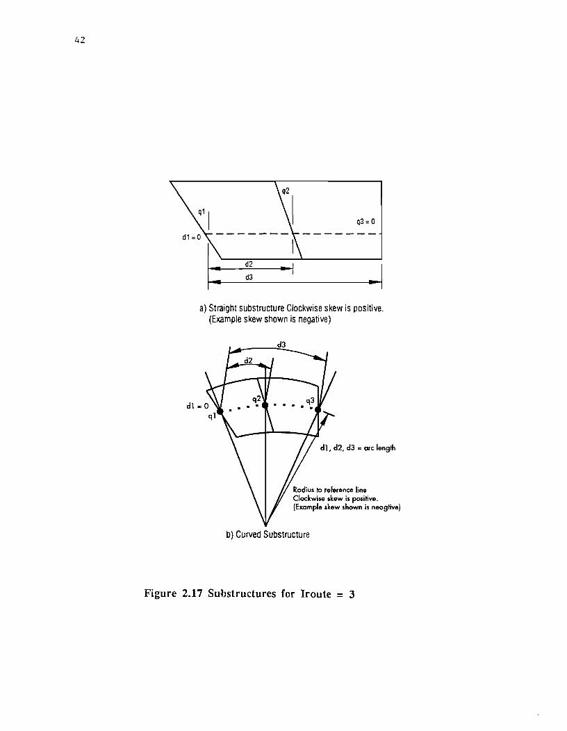
42
q3 = 0
I~ d2
d3 ~I a) Straight substructure Clockwise skew is positive.
(Example skew shown is negative)
dl, d2, d3 = orc lenglh
Rodius to reference line Clockwise skew is posi~ve. (Exomple skew shown is neog~ve)
b) Curved Substructure
Figure 2.17 Substructures for Iroute 3

43
D) SLIGHT SKEW MESH GEOMETRY
The following is input for each transverse rows of nodes at the bottom flange
locations.Caution should be shown if the mesh size was automatically determined. For
further infonnation see Figure 2.17.
LINE COLS. TYPE
1
LINE 1
24.5
1- 10
11-20
F Reference line distance until transverse row of nodes:'-ft- (Dsks)
F Skew angle of interior row of nodes. Positive is measured as clockwise. The angle is
measured from the radius through the node. -degrees- (Dslce)
E) ADDmONAL LOADS
COLS. TYPE
1-5 I
6-10 I
11-15 I
21-30 F
31-40 F
41-50 F
51-60 F
IROUTE=4
Loads are input by elements. Each line of data is superimposed on loads that may exist
for that member. End this section by placing a zero in column one. Signs of additional
loads should follow element axis as shown in Fig. 2.3a, b and c.
OOF of forces for this element (i.e., 1 - 6) (Idof)
Substructure where this element is located. (Jsubld)
Element number. (Kelno)
Force at node I of this elemenL (P(1»
Force at node J of this elemenL (P(2»
Force at node K of this elemenL (P(3»
Force at node L of this elemenL (P(4»
This choice of substructure is used for severly skewed supports. Unlike the slight skew of supports, the
mesh for this substructure is not distorted. The assumptions are made that the diaphragms are intersected at
support locations over the girders. This assumption allows for many configurations for a skewed support as
shown in Figures 2.8, 2.9 and 2.19. Depending on the arrangement of the diaphragms, the supports can be located at
the ends of the substructure or at interior nodes as well. The assumption is still made that a substructure is defined
as the pan between two diaphragms. When there are many diaphragms between the first and last support, this type
of substructure must be used until all girders are supported. As for IROUTE = 3, the data for either IROU1E = 1
or IROUIE = 2 up to the data on additional loads must immediately precede the following inpUL
A) SUBSTRUCTURE INDEX
LINE COLS. TYPE
1 1- 5 I = 4 , Type of substructure. (Iroute)
B) INPUT DATA FOR EITHER SECTIONS 2.4.2 OR 2.43
Any additional loads still must be input at the end of this section.

44
\ \ \
\ \ \ a) Slight skew bridge with non-radial diaphragms
and diaphragm over interior support
\ \ \ "" \
\.
\ \ \ \
b) Slight skew bridge with interior radial diaphragms and no diaphragm over interior support
End/" diaphragm
c) End support slightly skewed end diaphragms not radial
Figure 2.18 Examples of Iroute = 3

"" Girder 1
Girder 2
Girder 3
Girder 4
a) One substructure for severely skewed support "'"
"'" Girder 1
Girder 2
Girder 3
Girder 4
b) Two substructures for severely skewed supports"'"
Figure 2.19 Example for Iroute = 4
45

46
C) SEVERE SKEW SUPPORT PLACEMENT
LINE COLS. TYPE
1 1- 5 I
6-10 I
Girder number which is supported along the starting diaphragm.(Nge)
Girdf'J' number which is supported along the ending diaphragm. (Ngs)
D) ADDmONAL LOADS
LINE COLS. TYPE 1 1-5 I
6-10 I
11-15 I
21- 30 F 31-40 F
41-50 F
51-60 F
2.4.6 IROUfE=S·
Loads are input by elements. Each line of daIa is superimposed on loads that may exist
for that member. End this section by placing a zero in column one. Signs of additional
loads should follow element axis as shown in Fig. 2.3a, b and c.
DOF of forces for this element (Le .• 1 - 6) (Idof)
SubstruClUre where this element is loca1ed. (Jsubld)
Element number. (Kelno)
Force at node I of this element (P(I))
Force at node J of this element (P(2))
Force at node K of this element (P(3))
Force at node L of this element (P(4))
This substrut:ture is 'used when the geometry of the 'bridge does not lend itself to one of the previously
specified substructures. This substtucture is then placed after the previous substructure and all renumbering of the master nodes is done automatically. Care must be taken in numbering the nodes. Any nodes which bordf'J' on a
substructure that is generated must be numbered consecutively from lowest to highest Also, all nodes specified
must have elements connected to them. All live loads due to trucks or lanes must be input for this substructure.
A) SUBS1RUCfURE INDEX
LINE COLS. TYPE
1 1- 5 I = 5 • Type of substructure. (lroute)
B) CONTROL CARDS FOR TInS SUBS1RUCTURE
LINE COLS. TYPE
1 1 - 5
6 -10
I
I
11 -15 I
16- 25 F
Number of elements for this substructure. 200 maximum. (Noel)
Number of points for this substructure. 162 maximum. (Nopt)
Number of times this substructure is repeated consecutively. 16 Maximum. (Nv)
Reference radius. -ft- See Figures 2.4, 2.20, and 2.21.
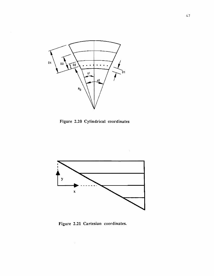
47
Figure 2.20 Cylindrical coordinates
L:------.~ x
Figure 2.21 Cartesian coordinates.

48
LINE
1
C) ELEMENT NODE NUMBERS FOR TIllS SUBSTRUCTURE
COLS.
1 - 5
6 -10
11-15
16-20
TYPE
I
I
I
I
One line per element is required for this inpuL Element node numbers should be
numbered counter-clockwise as shown in Figures 2.3a, 2.3b and 2.3c. For elements with
less than four nodes, leave the remaining node numbers blank.
Element nodal point I
Element nodal point J
Element nodal point K
Element nodal point L
D) CYLINDRICAL COORDINATES
Used if the Reference radius input above is larger than zero. One line per point is
required as described below. If the reference radius is input as zero, skip this section. See
Figures 2.4b and 2.20 for further information.
LINE COLS. TYPE
1
LINE
1
1 - 5 I
11-20 F
21- 30 F
31-40. F
Point number.
Distance, D , form Reference circle. -Ct
Angle in degrees, A, from Y-axis.
Distance, Z , from X-Y plane.
E) CARTESIAN COORDINATES
COLS.
1- 5
11-20
21- 30
31-40
41-45
46-50
51- 55
56-60
61-65
66-70
TYPE
I
F
F
F
F
F
F
F
F
F
Used if the Reference radius is input as zero. One line per point is required as described
below. See Figures 2.4a and 2.21 for further information.
Point number.
Cartesian X- coordinate. -ft
Cartesian Y - coordinate. -ft
Cartesian Z- coordinate. -Ct-
Component in X- direction of unit vector S1 •
Component in Y - direction of unit vector S1 ••
Component in Z- direction of unit vector S1 . ••
Component in X- direction of unit vector S2 . ••
Component in Y - direction of unit vector S2. •
Component in Z- direction of unit vector S2 ••
• is usually input as 1.0
.. is usually input as 0.0
NOTE: S1 and S2 are surface coordinates and are described in detail in CFHR Report
23 - 3F and have the same meaning here.

LINE
1
LINE 1
LINE
1
49
F) ELEMENT TYPES AND MATERIAL PROPERTIES
Web Elements
COLS. TYPE 1-5 I
6-10 I
11-15 I
16-20 I
21-30 F
31-40 F
41-50 F
51-60 F
61-70 F
Slab Elements
COLS. TYPE 1-5 I
6-10 I
11- 15 I
16-20 I
21-30 F
31-40 F
41-50 F 51-60 F
61-70 F
Beam Elements
COLS. TYPE 1- 5 I
16-20 I
21-30 F
The plate element can be either a triangle or a quadrilateral with the correct input for
nodes and triangles. The distinction is made between a flange and a beam element for
ease of input and output only. The flange element is assumed rectangular and the inertias
are calculaled from the thickness and width. The output for the flange elements are in
terms of sttesses and the output for the beam elements are in terms of forces. One line
per element is required as described below. Use the same order of elements numbered in
section 2.4.6, part C.
Number of nodes per element.
Number of sub triangles of quadriJatelal.
= 0, if CLST is used for membrane stiffness.
= 1, if QM5 is used for membrane stiffness.
= 0, type of plate element.
Modulus of elasticity in x-axis direction. -ksi-
Modulus of elasticity in y-axis direction. -ksi-
Thickness of element -in-Poisson's ratio for sttess in x-axis direction.
Element unit weight -kef-
This should be input as negative for dead loads.
Number of nodes per element.
Number of sub triangles of quadriJateral.
= 0, if CLST is used for membrane stiffness. = I, if QM5 is used for membrane stiffness.
= 1. type of plate element Modulus of elasticity in x-axis direction. -ksi-
Modulus of elasticity in y-axis direction. -ksi-
Thickness of element -in-
Poisson's ratio for stress in x-axis direction.
Element writ weight -kef-
This should be input as negative for dead loads.
= 2. Number of nodes per element.
= O. Type of beam element Modulus of elasticity. -ksi-

50
LINE COLS. TYPE
31-40 F
41- SO F
51- 60 F
61-70 F
71- 80 F
Flange Elements
LINE COLS. TYPE
1 1- 5 I 16- 20 I
21-30 F
31-40 F
41-50 F
51- 60 F
61-70 F
71-80 F
Cross-sectional area. in2-Shear Modulus multiplied by torsional moment of inertia. -k in2- (Gn
Element unit weight. - k I ft -This should be input as negative for dead loads.
Inertia -Y. -in4-Inertia -z. -in4-
= 2. Number of nodes per element
= 1. Type of beam element
Modulus of elasticity. -ksi
Cross-sectional area. -in2-
Shear Modulus multiplied by torsional moment of inertia. -k in2_ (Gn
Element unit weight- k I ft - This should be input as negative for dead loads.
Thickness of flange. -in
Width of flange. -in-
Rigid Link Elements
LINE COLS. TYPE 1 1 -5
16-20
I
I
= 2. Number of nodes per element
= 2. Type of beam element
All the remaining properties are intemally set in the program. The rigid lin1c: connects
the top flange to the concrete slab and functions as a shear stud
G) NUMBER OF ELEMENTS BELONGING TO EACH SUBSlRUCTURE
L1NE COLS. TYPE 1 1- 5
6 -10
I
I
76- 80 I
Number of elements for substructure 1.
Number of master nodes for substructure 2.
Number of master nodes for substructure 16.
The fll'St value should be the number of elements and all additional values should be the
ne~ve of the number of master nodes for the element See section 2.5.16 and examples
in Chapter 4 for further information.
H) CON1ROL CARDS FOR TIllS SUBSTRUCTIJRE
LINE COLS. TYPE 1 1- 5 I Number of master nodes for this substrucwre.
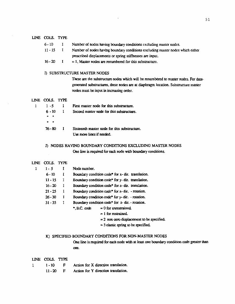
LINE COLS. TYPE
6 - 10 Number of nodes having boundary conditions excluding master nodes.
11 - 15 I
16 - 20 I
Number of nodes having boundary conditions excluding master nodes which either
prescribed displacements or spring stiffnesses are input.
= 1. Master nodes are renumbered for this substructure.
n SUBSTRUCTURE MASTER NODES
These are the substructure nodes which will be renumbered to master nodes. For data
generated substructures. these nodes are at diaphragm location. Substructure master
nodes must be input in increasing order.
LINE COLS. TYPE
1
LINE
1
1 -5 6 -10 .. ..
I
I
76- 80 I
First master node for this substructure.
Second master node for this substtuctllre.
Sixteenth master node for this substructure.
Use more lines if needed.
J) NODES HAVING BOUNDARY CONDmONS EXCLUDING MASTER NODES
One line is required for each node with boundary conditions.
COLS.
1- 5
6-10
11-15
16-20
21-25
26-30 31- 35
TYPE
I
I
I
I
I
I
I
Node number.
Boundary condition code· for x- dir. translation.
Boundary condition code· for y- dir. translation.
Boundary condition code· for z- dir. translation.
BOlDldary condition code· for x- dir. - rotation.
Boundary condition code· for y- dir. - rotation.
Boundary condition code· for z- dir. - rotation.
• • B.C. code = 0 for unrestrained.
= 1 for restrained.
= 2 non-zero displacement to be specified.
= 3 elastic spring to be specified.
Ie) SPECIFIED BOUNDARY CONDmONS FOR NON-MASTER NODES
51
One line is required for each node with at least one boundary condition code greater than
one.
LINE COLS. TYPE
1 1 - 10 F Action for X direction translation.
11-20 F Action for Y direction translation.

52
LINE
LINE
1
LINE
1
LINE
1
COIS. TYPE 21- 20 F Action for Z direction translation.
31-40 F Action for X direction rotation.
41-50 F Action for Y direction rotation.
51-60 F Action for Z direction rotation.
L) INPUT REQUIRED FOR DATA GENERATOR PROGRAM
COIS. 1- 5
6-10
11-15
16-25
TYPE
I
I
I
F
Number of nodes for a data-generated cross-section at,a diaphragm location. (Nxnd)
Number of master nodes wilh boundary conditions for this substructure. (Nbc5)
Number of master nodes wilh prescribed displacements or suppon springs. (Lpgo5)
Reference line length for substructure. -ft- Used in global placement of truck and lane
loads. (Dcent5)
M) BOUNDARY CONDmONS FOR MASTER NODES FOR THIS SUBSTRUCTIJRE
COIS.
1· 5
6-10
11·15
16-20 21-25
26-30
31- 35
TYPE I
I
I
I
I
I
I
Master node number. This node number is lhe local node which will be renumbered to
the correct master node.
Boundary condition code* for x- dir. translation.
Boundary conditioo code* for y- dir. ttanslation.
Boundary condition code* for z- dir. translation.
Boundary condition code* for x- dir. - rotation.
Boundary condition code* for y- dir. - rotation.
BolUldary condition code* for z- dir. - rotation.
"'. B.C. code = 0 for unn:suained.
= 1 for restrained.
= 2 non-zero displacement to be specified.
= 3 elastic spring to be specified.
N) SPECIFIED BOUNDARY CONDmONS FOR MASTER NODES
One line is required for each node wilh at least one boundary condition code greater than
one.
COLS. TYPE
1-10 F Action for X direction ttans1ation.
11-20 F Action for Y direction transJation.
21-20 F Action for Z direction translation.
31-40 F Action for X direction rotation.
41-50 F Action for Y direction rotation.
51-60 F Action for Z direction rotation.

LINE
1
53
0) ADDmONAL LOADS
COLS. TYPE
1-5 I
6-10 I
11-15 I
21-30 F 31-40 F 41-50 F
51-60 F
Loads are input by elements. Each line of data is superimposed on loads that may exist
for that member. End this section by placing a zero in column one. Signs of additional
loads should follow element axis as shown in Fig. 2.3a. b and c.
DOF of forces for this element (i.e., 1 - 6) (Idof)
Substructure where this element is located. Osubld)
Element number. (Kelno)
Force at node I of this element. (P(I» Force at node J of this element (P(2»
Force at node K of this element (P(3»
Force at node L of this element (P(4»
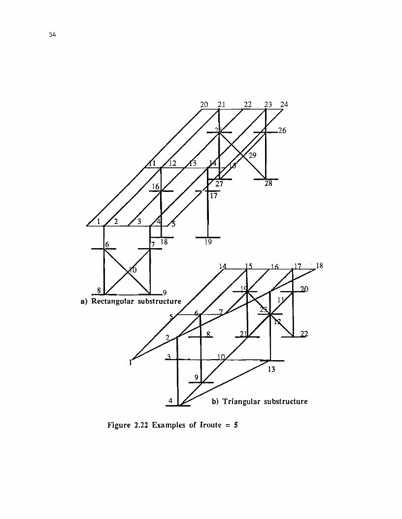
54
20 21 22 23 24
a) Rectangular substructure
1
b) Triangular substructure
Figure 2.22 Examples of Iroute = S

55
2.5 ADDITIONAL REMARKS
The following commentary should be used along with the documentation to aid in the preparation of
the input data. The examples in Chapter 4 can also help in understanding the documentation.
2.5.1 Control cards
The data generator automatically adds the half-diaphragms on the end of the bridge if the end
substructures are not input by hand. (Iroute = 5). The number of type of substructures (Nogp) is automatically
incremented and two new substructures are defined. The counting of the number of substructures for the support conditions and the erection process must not take these substructures into account. The number of
substructures between supports and for erection purposes should consider only the type of substructures that are
between diaphragms inclusive. For further clarification see Figure 2.8 and examples in chapter four.
The plotting routine (Ipl) will plot all the elements as viewed in both the XY and YZ planes. The
node numbering will be only for the first diaphragm cross-section in the YZ plane and the slab nodes in the XY
plane. This was done to avoid congestion on the plot. The plots of the concrete slab stresses by slab node are
also available if IPL equals 2. This is useful for a visual description of the slab stresses as well as the fact that
the slab stresses are only printed out at the midpoint of the slab elements.
The check prints (IdeO option outputs information that is mostly relative to the data generator and
related programs. The most important option is how deflections should be printed.: i.e., Idef = 0,1 or 2. If Idef
= 1 then deflections are printed out by master node. In most all cases this is at diaphragm locations. If Idef = 2 then deflections are also printed out by element. For large jobs there are a lot of elements and the output of
deflections will entail a lot more output. Many times the deflections by master nodes may be sufficient. If
there are any supports for local nodes as opposed to master nodes, then Idef needs to be set equal to 2 to
determine these reaactions.
The size of the mesh can be automatically generated. This should be used with caution since the
program may not generate a good mesh in all cases. Since the web depth is fixed, the mesh generator
determines the number of divisions along the reference line that will most likely give a square web element.
Knowing the longitudinal size of the elements, the mesh generator determines the number of transverse
divisions so that the concrete slab elements are most nearly square. The mesh generator is done only once for
the bridge so, for best results, the spacing of the diaphragms should not change too much longitudinally across
the bridge. Also for a better mesh size, the reference line should be located between the first and last girder of
the bridge. It may be recommended that the automatic mesh size generator be used in preliminary designs and
the user should determine the mesh size for the final computer runs.
2.5.2 Support Conditions
A couple of examples of the number of substructures per span are shown in Figure 2.8. A cantilever is
counted as a span. For supports done with IROUTE = 5, do D..Q1 count that support as dividing a span. If all
supports are input with IROUTE = 5, Then input a 1 for Nspan and a number greater than the total number of
substructures for Nsubbc. The number of substructures per span are used as a counting procedure to place the
supports in the data generator. When the supports are not generated then this special input is needed.
For data-generated substructures, the boundary conditions are internally set in the program. Only one
support is restrained in the horizontal planes. All other supports are supported in the vertical direction only.
The default support stiffness is 1.0 x 10 50 kips / inch. Other vertical support stiffnesses and initial

56
displacements can be input for each support. In this way, the effect of support settlements, rotations and
different spring stiffnesses can easily be analyzed. Support rotations can be analyzed assuming a linear
displacement for vertical displacements for the girders. The choice of boundary conditions for Iroute = 5 is up
to the user. Spring stiffnesses and displacements can also be input for all these supports.
2.5.3 Erection process The erection program uses superpostion to add up stresses for the construction stages. The old stresses
are written onto tapes and the option is given to add new stresses to the old stresses (Ircsum). The assumption
was made that during construction, the steel girders being placed already have the diaphragms and the bouom
bracing attached between them. Diaphragms and bottom bracing can be attached between two girders in later
stages by using the negative number of the girders to which they are being attached. The diaphragms and the
bottom bracing are assumed to be attached during the same stage however.
The erection of the bridge is actually done by analyzing the same bridge geometry but modifying the
material properties. Initially, the steel modulus is set equal to a small number and the density of the steel is
set equal to zero for girders not yet erected. At the erection of the girder, both the density and the elastic
modulus are set equal to the proper value. All subsequent erection stages have the correct modulus but the
denstiy of that girder is zero. Thus the theory of superposition of loads is ensured. The placement of the
concrete must be done by hand in the same manner. This was done so that full flexibility can be
accomplished in analyzing the construction process. The user can set the elastic modulus of concrete equal to
different values as the concrete cures and new pours are made on the bridge. However, the load of the
concrete should only be included in one stage. The erection process prints the sum of the stresses along with
the new stage stresses. The program does not use second order analysis by connecting a new girder to the
deformed shape of a previously erected girder. The load is placed on the bridge after the erection is finished.
It is thus assumed that a continuous connection occurs before the load is placed. The user should be
cautioned that the crictical point of loading may occur when the connection is pinned and pinning a
connection is not possible with this program.
The same procedure for adding erection stresses can be used to sum the stresses due to different
loadings with the only difference being that no erection stages are input (Irec = 0). In this way, dead load and
live load stresses can be summed by the computer. Load factors for the live load can be input and load factors
for the dead load can be taken account of with the proper densities.
2.5.4 Bridge Geometry IT the mesh size generator is not used, then the number of divisions between girders and diaphragms is
up to the user. Care should be taken in keeping the aspect ratio of the web element around 2.0. The aspect
ratio of the overhang element can probably be around 4.0 since it has much less structural importance. The
program calculates the aspect ratios of all four node plate elements and prints out the maximum and the
average aspect ratios. The aspect ratio for any element probably should not exceed 5.0 and the average aspect
ratio of all the plate elements probably should not exceed 4.0. Since there are no nodes between the flanges
for the web element, the aspect ratio might be most critical for this elemenL The number of divisions should
be decided upon considering both aspect ratio and computer solution time.
The reference radius is arbitrarily input by the user. A positive radius is dermed as one which curves
to the right as one goes from left to right on the bridge. A negative radius curves to the left. A straight

57
substructure is dermed as having a zero radius even though the radius is actually infinite. The spacing of the
diaphragms are dermed along this reference line. The thickness of the concrete is assumed constant for the
bridge. Wearing surface should be input as a surface load. 1be outer overhang is the one next to girder one as
shown in Figure 2.4b.
2.5.5 Girder The location of the girders is done with respect to the reference line. Girder one is input first and each
girder is input in increasing order. Girder one is dermed as the girder having the largest radius. For straight
substructures, girder one is on the left as one goes from left to right on the bridge. The web depth is assumed
constant for all girders at all locations. The web thicknesses can be changed at different substructures but the
web is assumed within a substructure. Average lOp and bottom flange thicknesses are input to set the location
of the flanges for the structure and does DOl have anything to do with structural element thicknesses or
properties. The properties of the beam elements are lumped at these locations as shown in Figure 2.6. This
allows much easier input and much better advantage can be taken of repeated substructures.
2.5.6 Diaphragm Three types of diaphragms are provided for by the data generator as shown in Figure 2.11. The bracing
configuration can be different at each end of the substructure by changing the bracing index. A substructure
can have K-bracing at the start and X-bracing at the end of the substructure. Only the number of different
types of bracing members have to be inpuL The properties of each member are then inpuL Half the area,
inertias and torsional moment of inertias are used so that the sum of these properties will be correct when the
next substructure is placed adjoining it A slight drawback to this system is the erection sequence when the
next diaphragms are not added. In this case, the stiffness of the brace at the free end is only half of its full
value. A description index is used to detennine the location of the properties of the diaphragm members. The
diagonals are 1 and 4, bottom horizontals are 2 and 5 and top horizontals are 3 and 6 as shown in Figure 2.11.
2.5.7 Bottom HorizontaJ Braces
The bottom braces are connected in between the bottom flanges at diaphragm locations. These braces
are all assumed to be the same type of member. The full properties are input since these braces are not
adjoining another substructure. The braces can be can be arranged in X-bracing or single bracing may be
different between any two girders as shown in Figure 2.12. If the bracing configuration changes from one
substructure to the next , then a new substructure type needs to be dermed. The user could make the choice of
modeling the bracing as X -bracing and then only one substructure type needs to be dermed.
2.5.8 Material Properties The material properties for concrete and steel apply to all the respective elements in the substructure.
All concrete elements in the substructure have the same moduli, poisson's ratios and density. The web,
flange, and beam elements also have the same properties. The properties of the rigid link are internally seL
The densities of the elements must be input as a positive value for gravity loads. The program then switches
the sign to match the global sign convention.
The slab can be modeled with orthottopic elements if different elastic moduli are used for the two
directions. Since the x-direction parallels the side ij in quadrilateral elements and this side is mostly tangent
58
to the radius, the elastic modulus in the x-direction corresponds closely to longitudinal bending. A different
elastic modulus can be input in a perpendicular direction to side ij. One poisson ratio is input corresponding to
the transverse displacement due to a stress in the x-direction. The poisson ratio in the other direction is
internally calcluated based on elasticity equations. Also, the shear modulus is internally calculated based on
approximations for an orthotropic material (5). The equation of the shear modulus for an orthotropic material
was taken as the following:
(1- V 21 X V 12) x 2 G=
1
(EIXE2)2" -V21 xE2
The most common application of orthotropic plates is over negative moment regions. Also, orthotropic
plates can be used for the slab load on the bare girder for dead load case one. When the longitudinal concrete
is considered ineffective, as in negative moment regions, the slab load is still carried transversely to the
girders as a one-way slab. Thus, the elastic modulus in the x-direction can be set equal to a small number and
the modulus in the transverse direction can be set equal to the correct value. Since the poisson's ratio loses
meaning in one-way action as with the case with very different elastic moduli, it is suggested the the poisson's
ratio be set equal to zero for these cases.
2.5.9 Slab Loads
Different curb loads are possible for the inside and outside curbs. The curb loads are smeared on the
respective overhang elements as an increase in density of the concrete slab. The curb load should include all
loading expected on the overhang such as curbs, sidewalks, railings or pedestrians. The surface load is applied
throughout the concrete elements as an increase in density. No patterned surface load is possible for one
substructure, but it is possible to change the surface load on a new substructure type. Negative loads are
downward.
2.5.10 Truck Loads
The input for the truck loading is very convenient. The global centroid location of the truck is
specified along with an impact factor, name and direction. The location of the wheels are referenced from the
centroid of the truck as shown in Figures 2.13 and 2.14. If the same truck is placed at a different location in
the bridge, then only the global location needs to be specified again. The same local wheel locations are used
if the variable IBID is set equal to one. It is thus advantageous to place all alike trucks in order so that the
least amount of input is required.
The reference line of the bridge at the truck reference point should be the same number as the
reference radius for that substructure. This number can be positive, zero or negative. The truck is assumed to
be straight going around a curve so that the wheel will not be exactly the same distance off the reference arc.
If the radius changes in the middle of the truck, then two trucks must be input with the input for each wheel
load for the respective radii. This does not apply to the end of the bridge in which any wheels off the end of
the bridge are ignored. The program also ignores wheels off the side of the bridge. In this case, the program
prints out a warning statement and the number of wheels off the side of the bridge.
If a truck is placed on a substructure that is input by hand (Iroute=5), then these wheel loads must
also be input by hand. The program determines the load to each node with the areas of each quadrilateral as
shown in Figure 2.14b. This loading is applied in a way general enough to be used for skewed meshes which
are in a curve. Because upward loads are positive, all truckloads must be entered as negative.

59
2.5.11 Lane loads
The lane loading is input in much the same way as the truck loads. The lanes are assumed to follow
the radius at the centroid. If the radius changes in between the lane load, then two lane loads must be input.
The concentrated loads are applied at a single point much the same way as a wheel load. The user must define
an equivalent concentrated load if a concentrated live load is desired. Only the upper left and lower right
comers are input for the lane loads. The program divides the distributed loads into many concentrated loads
and places these loads on the respective elements in much the same way the truck loads are placed. For lane
loads over skewed meshes or end supports the lane load should be place over the entire area desired and the
program will disregard any lane loads not over elements. Negative lane loads are downward.
2.5.12 Additional Loads
Any loading can be superimposed on any element by using this input. The degree of freedom for the
forces correspond to the local axis of orientation of the element. This is not the global degree of freedom of
the substructure. Thus, if there is a wind load on the web then the loads would be in the z - direction on the
element and DOF = 3. If there is more than one loading DOF on the element then a line for each DOF must
be input. As an example, if there are vertical loads and two moments then three lines of input are needed.
The user inputs the substructure where the element is located. The substructure number corresponds to
the repeated substructure number. If there is a load on the third substructure out of five repeated substructures
then the substructure where this element is located is three. This is independent of where these substructures
are in relation to the bridge.
2.5.13 Iroute = 2
This section is used so that only the changes from previous substructures need to be input. There is a
number corresponding to each parameter that can be changed. Thus, to change a value, input the number
corresponding to the parameter to be changed and the new value.
Many geometric parameters can not be changed since a constant cross-section is assumed for node
locations. An exception to this is the diaphragm configuration. It is possible to put K-bracing on one end of
the substructure and X-braCing on the other end. If this is desired then a new substructure needs to be defined
for the subsequent substructure. The reason is that the X-bracing and the K-bracing will not match when these
two substructures are adjoined together.
The automatic determination of the mesh size is only done once for the bridge. If the spacing of the
diaphragms change significantly then the number of divisions between diaphragms may need to be changed.
When any material properties are changed, all alike elements are affected. Additional loads are also possible
per section 2.5.2 part J.

60
2.5.14 lroute = 3 The slight skew substructure can be used with or without supports. If there are no supports then the
number of transverse rows until the girders are supported (Nsbc) should be input as zero. A few examples of
the use of a slight skew substructure are shown in Figure 2.18. The most common use would be a slight skew
at an end support in which the girders at the end are supported. Also, a common use would be at an interior
support in which the diaphragms are eithez radial or skewed with the suppon. It is possible to have a skewed
mesh for a curved substructure. In this case the degree of skew is measured from the radial line at the
reference line as shown in Figure 2.17. All girders are assumed to be supported between diaphragms. If lhis is
not the case, then either Iroute=4 or Iroute::: 5 must be used. Additional loads are also possible on slight skew
of substructures.
2.5.15 lroute = 4 A severe skew has been assumed to go from one girder to another at diaphragm locations as shown in
Figure 2.19. This may be quite a severe restriction but it was done in order to ensure a propel' generated mesh.
This assumption still allows quite a bit of flexibility as shown in Figures 2.19. If there are diaphragms between
the fust and last girder supports then Iroute = 4 must be called again for this second substructure. This type of
substructure must be repeatedly used until all girders are supported. See the examples in Chapter 4 for f~er
information. Additional loads are also possible for this substructure.
2.5.16 lroute = 5 This type of substructure is used when the geometry of the bridge does not lend itself to one of the
previously specified substructures. Two examples may be the best to present this section as shown in Figures
2.20 and 2.21. The fust example is a curved substructure and the second is a triangular substructure.
Cylindrical coordinates are used for Figure 2.20 and cartesian coordinates are used for the straight triangular
substructure. The node numbering should be consecutive when bordering a data-generated substructure as in
Figure 2.22. The nodal coordinates must match exactly in the x-axis and z-axis when it borders on a data
generated substructure. The user could run a trial data-generated substructure to determine these coordinates.
Five different elements can be input The web and slab elements can be either quadrilaterals or
triangles. If the element is a triangle it has three nodes and one subtriangle. If it is a quadrilateral, it has four
nodes and four sub triangles as shown in Figure 2.3. The distinction is made between a web and slab elements
for ease of input and output only. The program also offers two membrane stiffness elements. The QM5 should
be used for quadrilateral elements when the mesh is mostly regular. The CLST should be used if the element is
sevezely distorted or is a triangular element In most cases the QM5 is preferred for quadrilateral elements and
the CLST for triangular elements.
The distinction is also made between a rigid link, beam element and flange element for ease of input
and output only. The beam elements are used for the diaphragms and the output is in forces. The diaphragm
can be made a truss if the inertias and torsional rigidity are set equal to a small number or zero. The flange
elements are assumed to be rectangular with the physical properties internally determined. The output for the
flange elements is in stresses. The rigid link has the properties internally set in the program and the output for
them is in forces.
The input in part G for the number of elements belonging to each substructure is most important for
repeated substructures. If there is only one substructure then only the numbel' of elements for the substructure
61
must be input. The master nodes are global nodes and they describe how the substructures fit together. The
data-generated substructure uses the nodes at diaphragm location for master nodes. The master nodes in
Figure 2.22a could be 1-10 and 20-29. The master nodes in Figure 2.22b could be 1-4, 7, 10-13, and 14-23. For
repeated substructures, the second through the rest of the entries in line six (see Appendix, Sec. 2.4.6, Part G)
should be the negative number of the number of master nodes. For example, if there where three repeated
substructures as in Figure 2.22a then the input would be 34, -20, -20 since there are 34 elements and 20 master
nodes. The substructure in Figure 2.22b can not be repeated.
The control cards describe in more detail the master nodes for the program. The nodes that have
boundary conditions that are not master nodes are used if there is an interior support. If the substructure in
Figure 2.22a is supported in the middle at nodes 18 and 19 then the number of nodes having boundary
conditions that are not master nodes is two since nodes 18 and 19 are not master nodes. The boundary
conditions for each non-master node must be input in part J. The number of nodes which are not master nodes
that have prescribed boundary conditions (Lpgi5) must equal the number of nodes which have boundary
condition codes greater than one in part J.
Additional input is required for the data-generated program. The number of nodes for a data-generated
cross-section is assumed constant and it would be 10 for both Figure 2.22a and 2.22b since they both have 10
noo.es at a diaphragm location bordering a data generated substructure. The number of master nodes with
boundary conditions must also be input along with the restraints. The number of master nodes with prescribed
bondary conditions (Lpg05) must also equal the number of nodes which have boundary condition codes greater
than one in part M. The reference line length should be the arc length along the reference line. This is used
for global placement of the truck and lane loads. All live loads must be input in the section for additional
loads. This applies to both truck and lane loads. Thus, if a truck is half on and half off a substructure as in
Figure 2.22 then the wheel loads must be resolved to nodal loads on the respective elements. Also, only the
wheel loads on the data generated substructure must be input. Again, all loads should have the signs
corresponding to the element coordinate system.
2.6 REMARKS IN GENERAL
This program actually was developed in three parts with the most of the work being done on pre- and
post- processors. Many things had to be adapted to the existing program. One of the things that was used was
master nodes. The master nodes in a general sense describe how the substructures fit together. In addition to
those master nodes, any nodes can be master nodes such as the nodes on the ends of the bridge. The master
nodes must be known for a substructure since the output of deflections is first output by master nodes and then
by elements. The way the program determines which local node is a master node is through renumbering. The
program automatically renumbers the respective local nodes to master nodes and outputs the renumbering
scheme.
Many assumptions as to the size of problems to be solved were made. If problems are larger than the
stated maximums then some guidelines to changing dimension statements are given in Appendix A.

62
2.7 SUGGESTIONS FOR THE APPROACH TO THE SOLUTION The approach to this program was to apply easy input to a rather complex problem while still
remaining flexible enough to handle many bridge types. Along this line, general guidelines in modeling are
described below.
1) Determine a preliminary design with approxilJl8le methods such as the V -load, similiar bridges
ele ..
2) Determine the number of substructures for each span. A subslrUcture is defmed as the part of the
bridge between two diaphragms as shown in Figure 2.2 .
3) Determine the number of different types of substructures. This is done by looting at changes in
flange dimensions, radii , diaphragm members and configuration, diaphragm spacing and
material properties of concrete and steel ele ..
4) Of these types of SubslrUctures, determine which can be generated by the data generator. It is to
the users advantage that as many substructures as possible be generated by the data generator.
Since this is the case, approximations in modeling might prove extremely helpful. Four of the
major approximations are in the flange dimensions, radius changes, concrete modulus and
diaphragm spacing. The flanges are assumed to change at diaphragm locations. This is almost
always not the case. The user must decide whether to continue or change a flange from one
diaphragm to the next. An alternative is to change the diaphragm spacing to coincide with
change in the flanges. The radius is also assumed to change at diaphragm locations. Since there
is generally not a sharp change in the radius, this assumption is not seen to be too critical.
The place where the concrete is ineffective, such as in negative moment regions, must also coincide with a
diaphragm. No reinforcement bars are included in the slab. Over negative supports the concrete modulus
can be set equal to the following equation:
E' = (Area of rehar X E concrete 2)/(Area of concrete X E steel)
The user can run a fully composite bridge and determine the area of concrete in tension. The user can then
set the concrete modulus in the appropriate places.
5) Determine how many alike substructures are repeated consecutively. It is also to the user's
advantage to repeat as many substructures consecutively for ease of input. The same
assumptions that apply in item 4 (above) can apply here.
6) Determine the refmement of the slab mesh. As a first approximation, one can take the spacing
of the diaphragms and divided it by the web depth. The number of longitudinal divisions is this
whole number. TIle number of transverse divisions between girders is the girder spacing divided
by the longitudinal division increment The idea is to get a more or less square mesh. Since the
web depth is fIXed, the slab elements size should be reasonably close to the web depth. The
difference should be less than about 2.5 to 1.0 and preferably less than 1.5 to 1.0.
7) Determine the physical parameters for each subslructure type as needed per the documentation.
8) Draw a sketch of the bridge layout and substructure types.
9) If some subslrUctures need to be input by hand then layout the nodal coordinates and the element
types. Determine the data needed per documentation for section 2.4.6.

63
10) Determine live loads. The location of the live loads for maximum effect could be roughly
determined with approximate methods such as influence lines or by the V-load method of Ref 14.
11) Run the dead load case with the longitudinal elastic modulus of concrete equal to a small
number. This simulatates the bare steel while still· getting the correct slab load to the girders. If
it is desired to sum subsequent load cases set Jrec and Ircsum equal to one.
12) Run the live load case with the appropriate concrete elastic modulus. If it is desired to sum the live load case with the previous dead load case then set Jrec equal to two and Ircsum equal to
one.
The solution time and cost will increase with an increase in the total number of elements. For
preliminary analysis, a coarser mesh and more approximations can be made. As the solution is fmalized, it
may be necessary to refine the mesh.


CHAPTER 3. OUTPUT INTERPRET A TION
3.1 INTRODUCTION
The output is described in this chapter from the input given in Chapter 2 This program was originally
developed as three separate programs GENPUZ, PUZF83 and RECPUZ. There are many check prints to
ensure that the correct infonnation is transferred between programs. In addition, there are many parameters
that are internally generated which are also check printed.
Two parameters that control the amount of output are IPL and IDEF. IPL equals one if plots of the XY
and yz cross-sections are desired. IPL equals two if a plot of concrete slab stresses in additon to the cross
section plots are desired. IDEF is used to echo the degree of output. If IDEF equals zero then only the
minimum of output is shown. This basically includes echo prints of input data and element stresses. No
deflections are output. If IDEF equals one then deflections by mastel" node and elements are output along with
echo prints of input data. If IDEF equals two then deflections and the maximum number of check prints are
output.
3.2 GENPUZ
The GENPUZ program reads in all the data and determines the element stiffnesses and load arrays. It
does this completely for each type of substructure.
3.2.1 GENPUZ Control Cards
The first output is two lines of labeling information for this run. This is followed with an echo print of
the data for the control cards in part A, line 3. The number of groups before half-diaphragms are added refers
to the number of groups or types of substructures input. This need not be the final number since the program
internally generates the half-diaphragms on the end of the bridge if required. NDOF at each joint has been
internally set equal to six. IGLB and IROT are variables used in PUZF83 and are internally set. The plotting
option (IPL) and output print option (lDEF) have been described above. The superpostion of stresses are used
in the construction stage or in different load cases if the stresses from the current computer run are to be
superimposed on the previous computer run. The rest of the check print should be the same as the data for the
control cards in Section 2.4.1. part A.
3.2.2 GENPUZ Erection Output
This section is output if the erection stage (Jrec) is greater than zero. Each steel stage number, along
with the starting and ending girder, and the starting and ending substructure, is output. This should be exactly
as input in Chapter 2.
3.23 GENPUZ Input Echo for Iroute = 1 to 4
The rust output is for the substructure type. (Iroute) The support conditions are only output once and
correspond to the input in Chapter 2. The substructure type value is renumbered if the half-diaphragms are
added on the end of the bridge. Thus, if the half-diaphragms are added on the end of the bridge, then the first
substructure type is the half-diaphragm. The second substructure type is the original number one substructure.
The bridge geometry, girder, and flange information should all be output the same as the input for Chapter 2.
65

66
The diaphragm member and the bracing index numbers should correspond to Figures 2.8a, b, and c. The
inertia-y and inertia-z should correspond to the local member axis as shown in Figure 2.3c.
The material properties and the slab loads should also correspond to the input for Chapter 2. The curb
load should be for the correct inside or outside overhang. The density and slab loads should be positive if
downward.
The truck location and direction is output for each truck centroid. The local distance from this
centroid is then output for each wheel. If IDEF equals one then the generated global location of the
concentrated loads are output. The load should be positive if downward. The truck is assumed straight going
around a curve so that the relative transverse distances and longitudinal distances are not the same in the
global coordinates. The global transverse location is the distance from the reference line if the substructure is
straight or the radius of the curve at the load if the substructure is curved. The global longitudinal location is
the length along the reference line as shown in Figure 2.10.
The lane load location is output for each centroid. The local distances are then output relative to the
centroid. If IDEF equals one then the global locations of the concentrated loads are output. The global
transverse location is the distance from the reference line if the substructure is straight or the radius of the
curve at the load if the substructure is curved. The global longitudinal location is the length along the
reference line. The upper left and lower right corners are also ouput for the distributed load. A negative load
is downward.
3.2.4 Nodal Coordinates
The nodal coordinates are output in either cylindrical or cartesian coordinates depending on the
substructure geometry. If IDEF equals two, then three values are output that are important to the program.
These numbers are counters for the number of nodes at specific points at a cross-section. They are used in the
bookkeeping process to determine element nodes, master nodes and support conditions.
3.2.5 Element Material Properties
The program generates the element material properties along with the node numbers. Each type of
element is output along with the calculated material properties. The beam elements should have the same
values as input in Chapter II except the density which is in units of kips per inch. The density of the web and
slab elements are in units of kips per inch cubed. The elastic moduli for the web is assumed to be the same in
both directions while different elastic moduli for the slab can be input. Only one poisson ratio is printed out
in the interest of space but the poisson ratio in the y-axis direction is calculated based on elasticity equations.
The area, GJ, Iy and Iz of the flange elements are all calculated based on a rectangular plate with the axis as
shown if Figure 2.3.c. The density is in units of kips per inch. The stud properties have been internally set
with no density.
3.2.6 Element Node Numbers
The element node numbers should correspond with the nodal coordinates, the element type, and the
element material properties. The number of elements, nodes, and repeated substructures are then output as a
check.

67
32.7 Aspect Ratio TIle aspect ratio of the plate elements are calculated for the user's information only. Error statements
are printed if the maximum aspect ratio exceeds five or the average aspect ratio exceeds four. These values
are set to ensure that the fmite elements give valid answers. If the aspect ratio is too large, then the user must
redefme a mesh.
32.8 Master Node Information
The master nodes for a data-generated substructure have been defined as the nodes at diaphragm
cross-sections. Thus the master nodes correspond to the beginning and ending of the substructure. TIle number
of master nodes should be twice the number of nodes for a cross-section with diaphragms. The number of
nodes having boundary conditions, excluding master nodes, may be greater than zero for substructure types for
Iroute = 3 and 4. TIlese nodes that have boundary conditions may be in the interior of the substructure and are
not master nodes. If IDEF equals two then a check print is made if the nodes are renumbered. If interior nodes
have boundary conditions then the local node and the boundary conditions are printed.
The substructure local nodes are renumbered to master nodes. The master nodes are used by the
program to put the substructures together into a bridge. The user should be aware that master nodes are used
and that the deflections are printed out by master nodes as well as element nodes.
32.9 Superimposed Loads
All superimposed loads due to truck, lane or any additional loads are printed OUL The substructure
number corresponds to the repeated substructure number and not the number of substructures in the bridge. The
OOF and the local node number corresponds to the local element axis. Local node 1 corresponds to node i for
example. The load direction also corresponds to the local axis as shown in Figure 2.3a, b, and c. All slab
loads are negative downward.
32.10 GENPUZ Input Echo for Iroute = 5 Much of the output is the same for a substructructure input by hand and a data-generated one. There
is, of course, more input required and this is echoed in the program for daIa verification.
The number of elements belonging to the substructure are output if IDEF equals two. This data is part
of a larger array which is output at the completion of GENPUZ. The number of master nodes for this
substructure and the number of nodes having boundary conditions excluding master nodes should be as input in
part H for Iroute = S. The substructure nodes chosen to be master nodes should be renumbered and the new
master nodes should be shown. All the rest of the input as per partS I through 0 for Iroute = 5 should be
output exactly as inpUL
3.2.11 Substructure Assemblage Information The substructure assemblage information echos input that is required for the main solver PUZF83.
The fIrst five items output if IDEF = 2 are preset values in the program corresponding to the maximum size of
arrays possible for solution. The number of master nodes with boundary conditions should be for the entire
bridge. If IDEF = 2 then an echo of the print options is given. The fust five values are check prints for
PUZF83 and they should be preset equal to zero. The value of IPE should be the same as IDEF. The

68
maximum number of master nodes, the total number of elements, and the total number of substructures
correspond to the entire bridge.
The number of elements per substructure follows the description if part G for Iroute = 5. If the number
is positive then this should be the number of elements for that substructure. If the number is negative then the
number should be the number of master nodes for the substructure. The boundary restraints are internally set
and should correspond to the entire bridge.
3.3 PUZF83
PUZF83 is the main solver of the program and detennines the nodal displacements. The first data
listed for PUZF83 should be the same as the substructure assemblage infonnation at the end of GENPUZ. The
data are written on a tape and this is a check print to make sure that the data were passed correctly.
3.3.1 Echo Print of Master Nodes
The next output if IDEF equals two is a check print on the number of substructures. This is then
followed by the number of elements per substructure (lsub) as described in GENPUZ. The rest of the output for
this section is verification that data was read correctly by PUZF83. The main thing that the user should check
is that the nodes are renumbered to the correct master nodes and the boundary conditions are correct.
3.3.2 Storage Requirements
The storage required is shown for the user's infonnation on solution size. The user should look at
these numbers and make sure that they are less than the values set in section 3.3. Also, the user can get an
idea of the size of the problem that is trying to be solved.
3.3.3 Computation Effort in Reduce
This section is printed out if IDEF equals two. This section shows how efficiently the buffer size is
used in processing the solution.
3.3.4 Deflections by Master Nodes
The Deflections are output by master node if IDEF is greater than or equal to one. The deflections are
printed out starting with the last substructure and working backward. The deflections are printed out in
increasing order starting with the lowest master node number for that substructure. The renumbering
infonnation in section 3.2.8 should be used for ease of interpretation. The reactions can be detennined with the
boundary condition infonnation in section 3.2.9. The default spring constant of 1.0 x 1050 was used at all
supports where prescribed displacents or springs were not input. Thus, to get the reactions, find the vertical
deflection at the master node which is supported and multiply by the spring constant. The reaction is then in
kips.
3.3.5 Check Print for Isub and Jsub
This check print is done if IDEF equals two. Isub should be the same as in section 3.3.1. The positive
numbers of Jsub should be the number of repeated substructures for each substructure type. The negative

69
numbers should be the number of elements for the substructure. The output for Jsub is in reverse order of the
substructures.
33.6 Deftection by Element
The deflections by element are output if IDEF is greater than or equal to two. The deflections are
output by all alike elements for each repeated substructure. For example, it is easy to tell the variation of the
deflection of the boUom flange for one substructure type as that substructure is repeated across the span since
the deflections are printed out all in order. The output across the row are printed out the same as for the master
nodes, i.e. x, y, z, rot-x, rot-y, and rot-z. The first line of deflections correspond to node i, the second line
corresponds to node j and so on. The axis of orientation at the node is in the direction of the surface
coordinates for that elemenL
33.7 Solution Time
The solution time should be used by the user in much the same way as the storage required. The user
can determine how to cut down on the solution time by keeping track of the time in various modeling schemes.
3.4 RECPUZ
Recpuz determines the stresses in the elements. The first output should be the number of groups of
substructures. If this is a construction sequence, and stresses are to be superimposed, then the disk fIle
number of the current stresses and the disk ftle used for superimposed stresses are printed ouL These disk ftles
should alternate with each load stage. The user has the option of plotting the concrete slab stresses at each
node if IPL was set equal to 2.
3.4.1 Stresses
The output of the stresses are broken up into five groups for ease of interpretation. The output of
stresses and forces for all the elements are with respect to the local member axis as shown in Figure 2.380 b,
and c. The forces are printed out for the rigid link and the diaphragm beam elements. The user can resolve
these forces into stresses with the respective element properties. The stresses for the flange elements are
printed out based on a rectangular section. The sigma x -YY and sigma x -ZZ are the strong axis and weak
axis bending stresses relative to the center of the flange as shown in Figure 3.1. The torque is only relative to
the nodes of the member and not to the entire girder as a whole. The stresses at the midpoint of the web and
slab elements are output for the top and bottom of the elemenL The user is cautioned that these stresses are
at the midpoint and not at each node. The slab stresses at each node can be output if Idef equals two. These
stresses are the same as the ones plotted.
The summation of the load case stresses or forces are printed out directly below the stresses or forces
of the current erection stage. This is indicated with the word "sum" next to the element number.
The plot of stresses are the average stresses at each node for each substructure. The stresses at the
borders of two substructures may not be exactly the same due to this averaging. It is up to the user to average
these stresses.

70
3.5 OUTPUT SUMMARY
The bridge geometry, loadings. and material properties are determined and output in the rust pan of
the program. Deflections by master node and by element are then output for the bridge, if desired. The
stresses by element are then given along with summation of stresses from the different load stages. Plots of
each substructure type in the XY and yz cross-section are available along with plots of the average slab
stresses. All the output is given in a space that is able to be trimmed to a neat 8-112 by 11 paper size.

M· ....... )'1
Figure 3.1a Beam element axes orientation
nodek
node 1 nodei
Figure 3.1b Plate element axis orientation
71
nodej


CHAPTER 4. EXAMPLE PROBLEMS
4.1 INTRODUCTION
Six example problems will be described in this chapter to demonstrate both the input procedure and
the versatility of the program. They are:
1) Simple span, two-girder curved bridge with a radius of 500 feet.
This example will be shown for both a dead load noncomposite case and a truck load case.
2) Three-span, four-girder curved bridge with a radius of 1,145.9 feeL
3) Two-span, three-girder straight bridge with severely skewed interior supports and radial end
supports.
4) Two-span, three-girder straight bridge with all supports severely skewed.
5) Two-span, four-girder curved bridge with all supports slightly skewed. The radius and diaphragm
spacing also changes for the bridge. This example will be shown for a dead load noncomposite
case, a two truckload case and a two lane load case.
6) Two-span, four-girder curved bridge with reverse curvature and all supports slightly skewed. This
example will be shown for a dead load noncomposite case, a two-truck load case and a two-lane
load case.
4.2 EXAMPLE 1
The first example is a simple span, two girder bridge with a radius of 500 feeL This problem is
probably one of the easiest ones for this program and it is also part of the example problems used to test the V
load and finite element programs. Cross-section and plan views are shown in Figure 4.1.
Two load cases are to be run for example 1.
Run dead load of concrete and steel for a noncomposite geometry.
Run live load of an HS20 - 44 truck going forward with the middle wheels at 54 feet from the left end of the
road as shown in Figure 4.2. The following is given for the example:
Centerline span length = 100 feeL
Centerline radius = 500 feeL
Diaphragm spacing = 20 feeL
Concrete slab thickness = 7.5 inches.
Slab overhang = 3.0 feet each side.
Girder spacing = 6 feet.
Top flange = 0.5 x 10.0 inches.
Bottom flange = 0.875 x 10.0 inches.
Web = 50.0 x 0.375 inches.
X- bracing with top horizontal member.
Area of diagonal diaphragm braces = 2.860 in2.
Area of horizontal diaphragm braces = 5.18 in2.
Elastic modulus of steel = 29,000 ksi.
73

74
Reference radius = 500 ft
-,-a) Plan view of Example 1
3' 3 ' 3'
50.0 x 0.375
0.875 x 10.0
A = 2.86 b) Section A.A of Example 1
Figure 4.1 Example 1

1-- -14 ft
c::::::J 16 k --
c::::::J 16k
a) Truck example
Global long. co-ord = 54 ft (arc lenglb)
.. t .. 14 ft "'1
c::::::J ~ 16k 4k 3 ft
+ -3 ft
c::::::J 16 k 4k
Reference radius = 500 ft
b) Truck placement for Example 1
Figure 4.2 Live load for Example 1
75

76
Elastic modulus of concrete = 3,625 hi.
Density of Concrete = 0.150 k / ft3.
Density of Steel = 0.490 k / ft3. Poisson ratio for concrete = 0.17.
Poisson ratio for steel = 0.30.
42.1 Dead Load for Example 1 The following is a guide for preparing the data for example 1. A listing of the input is given in
Appendix B. The first two lines are description lines for this program run. For the control cards, the number of
groups equals one since the bridge has a constant cross-section. This number will automatically be increased
to three when the half-diaphragm substructures are added at each end of the bridge. IDEF should be set equal
to 1 if a print-out of deflections by master nodes is desired. The next thing that is considered is that the run is
for the dead load and these stresses will be superimposed on the live load stresses. Since this is the first load
case, JREC should equal I. Also, since the live load stresses are going to be added to the dead load stresses
in a future run, IRCSUM should equal 1. IRCSUM tells the program to store the stresses on a disk me and to
read any old stresses. Load factors for the dead load can be taken into account with the material densities
but for this simple case the live and dead load factors equal 1.0 .
Since there is one lOO-foot span, and the diaphragm spacing equals 20 feet, then there are five
substructures for the span. The horizontal support restraints can be applied to either the fIrSt or last support. In
this case, the horizontal restraints are applied at the first support and NFIX equals zero. The rest of the data is
easily input Remember, the diaphragm properties must be divided by two since they are adjacent to other
substructures. Also, since this is a noncomposite section, KOMP should equal 1 and the concrete modulus
must be set equal to a small number like 1.0 hi. KOMP sets the concrete slab stresses equal to zero and
makes the rigid link a truss element so the studs are less effective.
422 Truck Load For Example 1 The live load must be run after the dead load run. To run the live load, set JREC equal to 2. To make
the bridge composite set KOMP equal to zero and set the concrete modulus equal to the proper value. Also,
the density of the steel and concrete needs to be set equal to zeco so that the proper stresses are superimosed.
To signify that a truck is to be input, set ZLIVLD equal to 1.0. Input the correct geometry of the truck as
shown in Figure 4.2. The location of the truck centroid is arbitrary but is usually easier if it is placed at the
truck centerline.
The live load is run and the sum of the stresses is printed out below the stresses due to the truck only.
If any error OCClU'S, increase IDEF equal to two and check the global placement of the concentrated loads.
Remember, the truck is assumed to be straight when going around a ClU'Ve.
43 EXAMPLE 2
The bridge for example 2 is shown in Figure 4.3 and Figure 4.4 and represents an example of a
highway bridge sent from the Houston Bridge Division. This three span, four girder bridge example was used
because two other computer programs have been run on the bridge and the results could be verified. Also, the
bridge is quite simple in geometry but still represents a typical design case. A listing of the input data is given

77
5 degree curve \ 12 bays @ 15.3929 ' 7 bays @ 15.3929 I
Figure 4.3 Plan view of Example 2
symmetrical
18 x 1 18 x 3 18 xI t
72 x 9/16
18x1.5 18x2 18 x 1.5 18 x 3 18 x 1.5 18 x 2 I
I . 3 bay.sl 4 bays 1 3 bays I 4 bays 13 bays 12 bays!
-'4 .-4 .... .·4 •. '4 1It·4 "'1
Figure 4.3b Elevation view of typical girder for Example 2
Area = 3.05 in2
Figure 4.4 Cross-section of Example 2
78
in Appendix B. Run the dead load due to concrete and steel for a noncomposite geometry since the procedure
for live load placement is similar to example 1. The following is given for Example 2:
Centerline span lengths = 185.15,210.0 and 185.15 feel
Centerline radius = 1,145.9156 feel (5 degree curve)
Diaphragm spacing = 15.3929 feel
Concrete slab thickness = 8.0 inches.
Slab overhang = 3.0 feet each side.
Girder spacing = 8 feet.
Area of diagonal braces of diaphragms = 3.05 in2.
Area of horizontal flange braces = 3.05 in2.
Area of diagonal bottom lateral brace = 2.81 in2
Elastic modulus of steel = 29,000 ksi.
Elastic modulus of concrete = 1.0 ksi. (noncomposite)
Density of Concrete = 0.150 k I f13.
Density of Steel = 0.490 k I ft3. Poisson ratio for concrete = 0.17.
Poisson ratio for steel = 0.30.
43.1 DEAD LOAD FOR EXAMPLE 2
This example is not much different than the frrst example except for two things. First, the flange
dimensions change. This means a new substructure needs to be defmed whenever the flanges change. Since
the flanges change 11 times, there are 11 groups of substructures. Since the flange dimension changes, an
average top and bottom flange thickness needs to be input for the vertical placement of the nodes. It is up to
the user to decide what an appropriate average should be. For this example, the average top and bottom
flange thicknesses were set equal to zero so the nodes would be placed on top and bottom of the 6 foot web.
The second difference is the presence of bottom flange diagonal braces. The program does not easily handle
braces which switch back and forth since a new substructure needs to be defmed everytirne this happens. An
easy way to model it would be to put x-bracing in each bay with half the area as shown in Figure 4.5b. In this
way the bracing configuration needs to be input only once and the stiffness and the dead weight is almost the
same. This method should not be used for fatigue loading since the stresses in the braces are probably not the
ones the model describes. Another way to model them is shown in Figure 4.5c in which the bracing direction
changes when a new substructure needs to be defmed anyway. The bracing can then go in one direction and
then switch near the inflection poinl
When the flanges change, the substructure geometry needs to be updated and the data from section
2.4.3 needs to be used. The two values that need to be changed are the number of repeated substructures (NY)
and the new flange dimensions. After each substructure is input, a zero is placed in column one to signify no
additional loads are placed on this substructure.

a) Designed braces for most economical results (A new substructure is defined for each bay)
b) Alternative X-bracing (Each bay has the same bracing configuration)
c) Alternative bracing scheme (Change bracing configuration when flanges change or at inflection points)
Figure 4.5 Examples of bottom horizontal bracing
79

80
4.4 EXAMPLE 3
Example 3 is a two-span, three-girder bridge with a severe skew at the interior support and radial end
supports. This example will show how to deal with a severe interior skew as well as specified support spring
stiffnesses. The bridge is shown in Figure 4.6 and a listing of the input data is given in Appendix B. The bridge
should be run for dead load due to concrete and steel for noncomposite geometry. The following is given for
example 3:
Centerline span lengths = 104 and 104 feeL
Centerline radius = 0.0. (straight)
Diaphragm spacing = 16.0 feeL
Concrete slab thickness = 7.5 inches.
Slab overhang = 3.0 feet each side.
Girder spacing = 8 feet 10 inches.
X- bracing without top horizontal member.
Area of diagonal diaphragm braces = 2.860 in2.
Area of horizontal diaphragm braces = 5.18 in2.
Elastic modulus of steel = 29,000 ksi.
Elastic modulus of concrete = 1.0 ksi. (noncomposite)
Density of Concrete = 0.150 k / ft3.
Density of Steel = 0.490 k / ft3.
Poisson ratio for concrete = 0.17.
Poisson ratio for steel = 0.30.
Support stiffness for girder 1 = 1.0 x 10 30 kips/inch.
Support stiffness for girder 2 = 2.0 x 10 30 kips/inch.
Support stiffness for girder 3 = 3.0 x 10 30 kips/inch.
Interior support horizontally restrained.
4.4.1 Dead Load for Example 3 This example is straightforward except for the support springs and the skew of the interior support As
described in Chapter 2, the order of the spring input must correspond to the order in which the supports are
numbered. Different values for the girder spring stiffnesses were used to better show the proper order of inpUL
The listing of the input including the proper order of the spring stiffnesses is given in Appendix B.
The interior skew is handled with the input from Section 2.4.5. The additional input required for
substructure 7 is only the starting and ending girder number. In this case the support starts at girder 3 and ends
at girder 1 as shown in Figure 4.6. The support at girder 2 is on the interior of the substructure so that there
needs to be two divisions between diaphragms so that a node is over girder 2. The number of substructures for
the frrst span is 7 and 6 for the second span. This is in keeping with the defmition of the number of
substructures per span given in Chapter 2. Since the interior support is horizontally restrained. NFIX equals 7.
The user must decide how to best model the change in flange dimensions for the interior skew. Even
when the supports are skewed. the flange properties must still change at a diaphragm location. This is quite a
severe restriction near negative supports since the flanges most likely do not change at diaphragm locations.
When there are skewed supports and flange changes, the user can place the flange changes at diaphragm
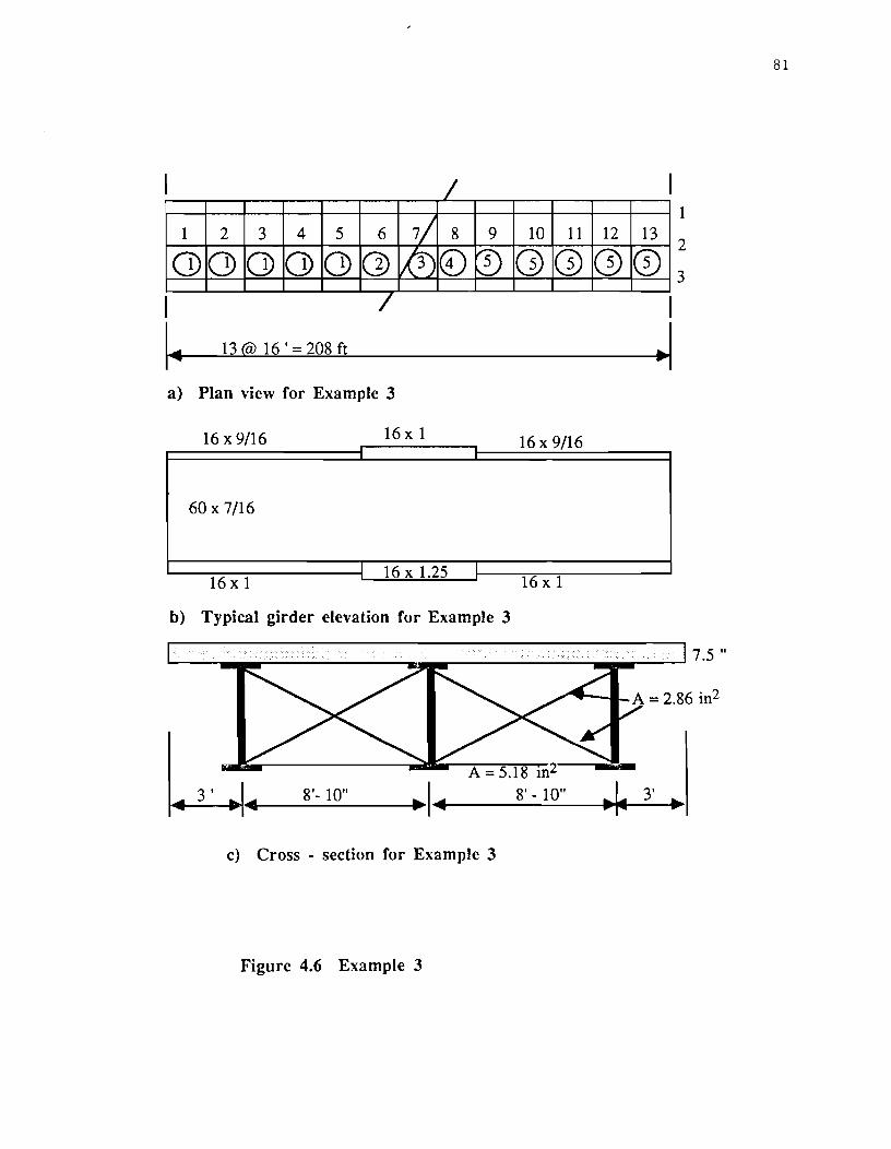
/
1 2 3 4 5 6 7/ 8 9
CD (J) CD CD Q) 0) l(3) CD tD I /
I~ 13 @ 16 ' = 208 ft
a) Plan view for Example 3
16 x 9/16 16 x 1
60 x 7/16
16 x 1 16 x 1.25 I
b) Typical girder elevation for Example 3
10 11
Q) G)
16 x 9/16
16 x 1
12
Q) 13
CD I
~
1
2
3
~--,.--~------~--~--~--------~----~~~
.~ 3' ..
c) Cross - section for Example 3
Figure 4.6 Example 3
81
7.5 "

82
locations or put dummy diaphragms (zero physical properties) at places where the flanges change. For girders
1 and 3 this is not a problem since the flange dimensions can change one bay away from each support For
girder 2 the flanges must change between substructures 6 and 8 or substructures 5 and 9. For this example it
was decided to change the flange dimensions for substructures 6 and 8. Thus. the flanges for the negative
moment region of girder 2 do not extend as far as girders 1 and 3.
45 EXAMPLE 4
Example 4 is similar to example 3 except the end supports are severely skewed and the interior
suppon is skewed across two bays instead of one. A listing of the input is shown in Appendix B. The bridge
should be run for dead load due to concrete and steel for noncomposite geometry. The following is given for
example 4:
Centerline span lengths = 111.434 and 111.434 feel
Centerline radius = 0.0. (straight)
Diaphragm spacing = 21.434. 16.0 feel
Concrete slab thickness = 7.5 inches.
Slab overhang = 3.0 feet each side.
Girder spacing = 8 feet 10 inches.
X- bracing without top horizontal member.
Area of diagonal diaphragm braces = 2.860 in2.
Area of horizontal diaphragm braces = 5.18 in2.
Elastic modulus of steel = 29.000 ksi.
Elastic modulus of concrete = 1.0 ksi. (noncomposite)
Density of Concrete = 0.150 k I f13.
Density of Steel = 0.490 k I ft3. Poisson ratio for concrete = 0.17.
Poisson ratio for steel = 0.30.
Suppon stiffness for girder 1 = 1.0 x 10 30 kips/inch.
Suppon stiffness for girder 2 = 2.0 x 10 30 kips/inch.
Suppon stiffness for girder 3 = 3.0 x 10 30 kips/inch.
Interior suppon horizontally restrained.
45.1 Dead Load for Example 4
The data generator can easily handle the interior suppon but it can not generate the triangular
substructures 1 and 13. For these special substructures the data from Section 2.4.6 needs to be inpul Pictures
of substructures 1 and 13 are shown in Figures 4.8 and 4.9. The input required for these sections is much longer
than others and the suppon springs have to be input for these end substructures. Also, the diaphragm properties
at the end of the bridge are no longer handled automatically in the program. Thus, the diaphragm properties
must have the full value at the end of the bridge and half the value when bordering a substructure.
The user must decide how to best model the concrete at the skewed suppon region. The
parallelograms which cantilever out will give very large displacements if the elastic modulus is set equal to a
small number. The use of the orthotropic properties might be especially useful in modeling the concrete of

/ /
8 9 10 11
/ 3
~1.4~ 21.43 I 11 @ 16 • - 176 ft I~ 1.~ 21.43 ~.~.~-~.~--------~----------------~.
a) Example 4 plan view
16x 9/16 16 xl 16 x 9/16
60 x 7/16
16x125 I 16x 1
5bavs 16 xl I .1... 2 bays t~II-II.I--__ ..loI.6..1i1:bwav~s ____ ---.., .. ~
b) Typical girder elevation
A=5.18 in2
~.-t"IiI'fI~.I----~8'--1~O:..-" ____ ...., ....... I~.I----~8'--...=.1~O·-· _.~1.1--"3:..-' -1 ....... 1
c) Cross - section for Examp]e 4
Figure 4.7 Example 4
83
1
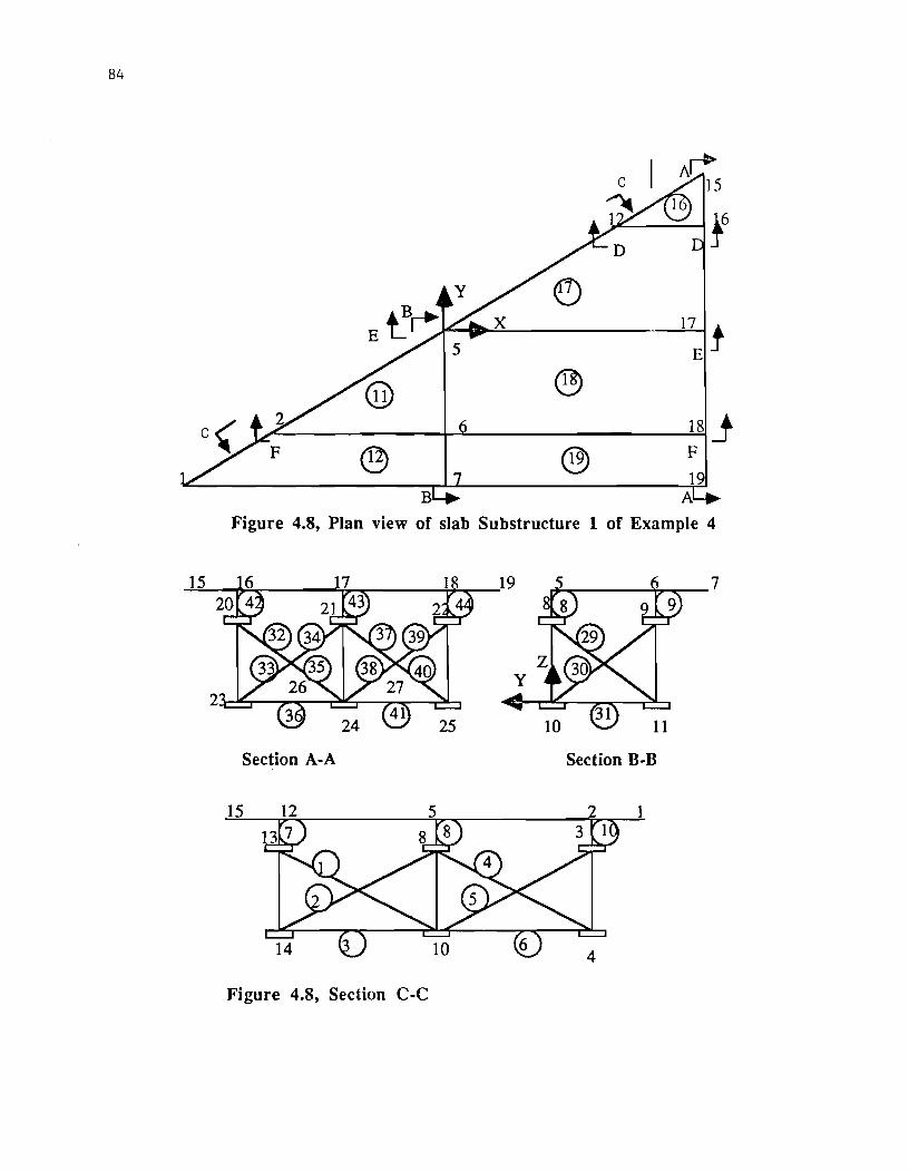
84
17 t E
® 18 j
® ® F
19 p.J
Figure 4.8, Plan view of slab Substructure 1 of Example 4
Section A·A Section B·B
15 1
Figure 4.8, Section C·C
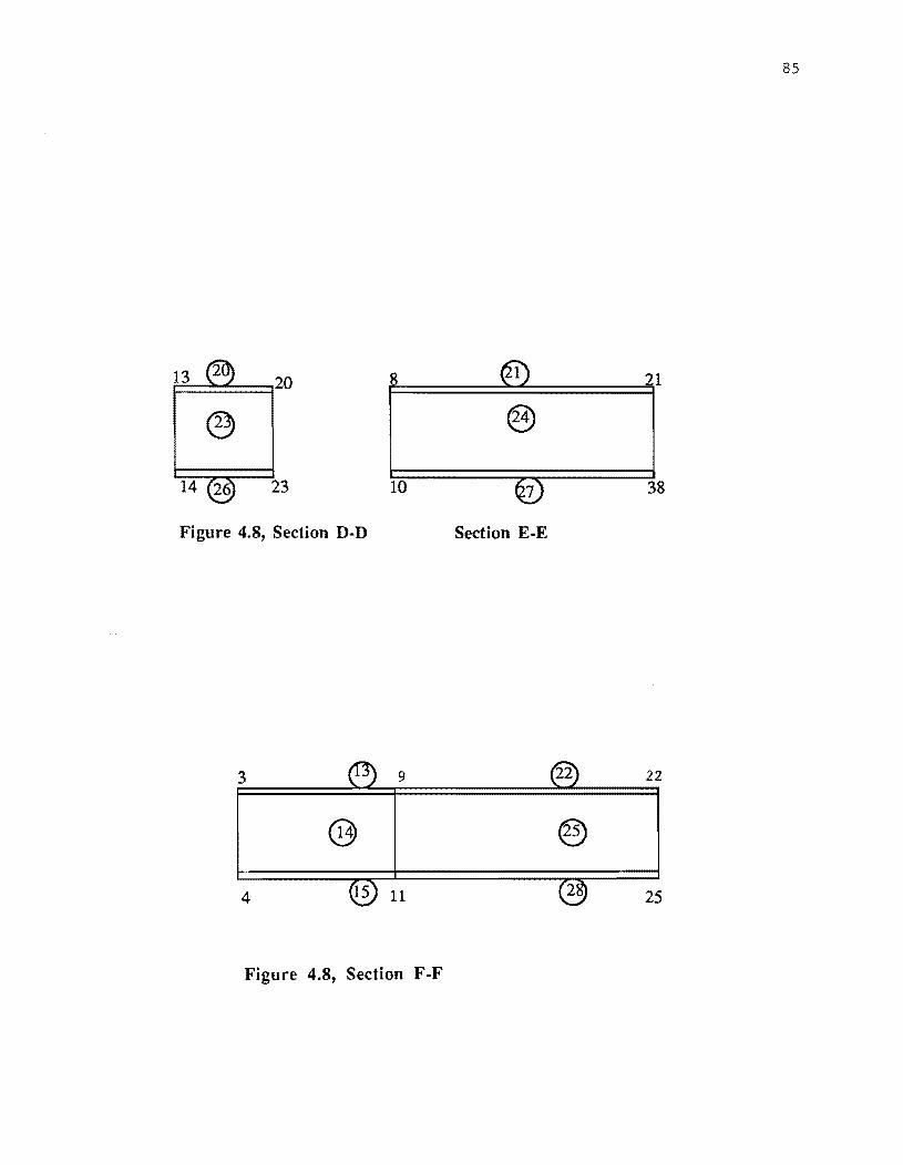
85
13 2 1 21 20
® @
14 26 23 10 7 38
Figure 4.8, Section D·D Section E-E
3 9 22 22
4 15 11 2 25
Figure 4.8, Section F·F

86
~A 1
F
~ 3
D
~B @ 17 (3
1
@ X
®
Figure 4.9, Plan view of slab for Substructure 13 of Example 4
17
Section A·A Section B·B
5~ __ ~~ ________ ~~~ ________ ~~~~24
Figure 4.9, Section C-C

87
8 2 19 21 5
® @
11 2 16 10 5 23
Figure 4.9, Section D-D Section E-E
6 18 20 33 26
®
9 4 22 35 27
Figure 4.9, Section F-F

88
substructures 1 and 13 as one way slabs. 1be triangular elements must use the CLST stiffness and 0 needs to
be input for these elements. 1be quadrila1eral elements still use the QM5 stiffness and 1 is input
1be number of substructures per span does not change from example 3 since the data generator counts
the number of substructures per span in the same way. One support still needs to be horizontally restrained and
the user can input this at the end supports or it can automatically be done by the data generator. Since the
interior support is horizontally restrained, NFIX = 7 and it is automatically done.
1bere is little less of a problem with the flange dimension changing since the flange changes can all
be the same length. Even when the supports are skewed, the flange properties must still change at a diaphragm
location. This is quite a severe restriction near negative moment supports since the flanges most likely do Dot
change at diaphragm locations. When there are skewed supports and flange changes, the user can place the
flange changes at diaphragm locations or put dummy diaphragms (zero physical properties) at places where
the flanges change. 1be diaphragm spacing has to be increased at the end supports since all the supports are parallel. When a custom substructure is adjacent to a data-generated substructure then the nodes much all
match up between substructures.
If a truck was placed on the end substructures then these concentrated loads must be input by hand. If
the interior support did not line up in such a nice way then substructures 6 and 7 would have to be input
according to Section 2.4.6 just like substructures 1 and 13.
4.6 EXAMPLE 5
Example 5 is a two-span, four-girder bridge with slightly skewed supports at all locations as shown in
Figures 4.10,4.11 and 4.12 This example shows the versatility of the program since, in addition to the skewed
supports, the flanges, the diaphragm spacing and the radius all change for the bridge. Run the dead load due to
concrete and steel load for noncomposite geometry. Also run two HS2().44 trucks with 14-foot axle spacing as
shown in Figure 4.13b. Load case 3 is two HS20-44 lane loads placed for maximum positive moment for span one as shown in Figure 4.13a. A listing of the input is given in Appendix B. The following is given for
example 5:
Centerline span lengths = 110.0 and 110.0 feet
Centerline radius for bays 1 - 8 = 500.0 feet
Centerline radius for bays 9 - 13 = 1,000.0 feet
Diaphragm spacing for bays 2-6 and 8-12 = 16.0 feet
Diaphragm spacing for bays 1,7 and 13 = 20.0 feet
Concrete slab thickness = 7.5 inches.
Slab overhang = 3.0 feet each side.
Soffit = 2.0 inches.
Girder spacing = 8 feet 10 inches.
K- bracing for diaphragms.
Area of diagonal diaphragm braces = 2.860 in2.
Area of horizontal diaphragm braces = 5.18 in2.
Elastic modulus of steel = 29,000 ksi.
Elastic modulus of concrete = 3,625 ksi.
Density of Concrete = 0.150 k I f13.

89
Figure 4.10 Plan view of Example S
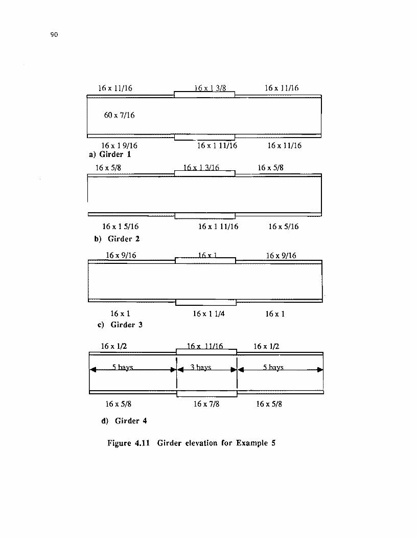
90
16 x 11/16
60 x 7/16
16x 19/16 a) Girder 1
16 x 5/8
16 x 15/16
b) Girder 2
16 x 9/16
16 xl c} Girder 3
16 x 1/2
16 x 5/8
d) Girder 4
16 x 1 3/8 16 x 11/16
16 x 111/16 16 x 11/16
1 h x 1 1/1 fi 16 x 5/8
16 x 1 11/16 16 x 5/16
1 h Y 1 16 x 9/16
16x 1 1/4 16x 1
16 x 1/2
16 x 7/8 16 x 5/8
Figure 4.11 Girder elevation for Example 5

Area = 2.86 in.2 ----,--,
A=5.18 in.2
3ft 8ft 10 in. 8ft10in. 8ft 10 in.
Figure 4.12 Cross-section of Example 5
3ft
7.5 in.
2in.
91

92
\ \
HS20 - 44 truck as shown in Figure4.2a
Figure 4.13a Truck placement for Example 5

4@ 5'
18k
5' ~~ ..... ~~~--~~~4---~
-5'
Figure 4.13b Lane load placement for Example 5
93

94
Density of Steel = 0.490 k I f13.
Poisson ratio for concrete = 0.17.
Poisson ratio for steel = 0.30.
4.6.1 Dead Load ror Eumple 5 1be data preparation for this bridge follows the other examples except for the skewed substructures.
There are seven groups of substructures as shown by the circled numbers in Figure 4.10. The bridge has two
spans and the second support can assumed to be horizontally restrained. From the defmition of the number of
substructures per span, there are 7 substructures for span 1 and 6 for span 2. NFIX should be equal to 7 to
horizontally resb'ain the interior support.
Substructures 1, 7 and 13 have slightly skewed supports and require additional input of Section 2.4.4.
The first thing to decide is the refmement of the mesh. Since the web depth is 5 feet, it seems reasonable to
have two divisions between diaphragms and one between girders. The mesh of the skewed substructures must
be decided by the user. The easiest decision is to use a linear change for the skew angle between the ends of
the substructure. A linear distance along the centerline can be used as the location of the interior row of
nodes. Shown in Figure 4.14 are examples of ways to divide up the mesh for substructures 1, 7, and 13.
The soffit is the distance from the top of the flange to the bottom of the concrete. The soffit and the
average top and flange thicknesses determine the vertical placement of the nodes. The user must determine
the average flange thicknesses for the entire bridge and determine an appropriate soffit dimension. The
average top flange thickness was set equal to 0.8 inches and the average bottom flange thickness was set
equal to 1.0 inches for this example.
For substructures 1, 7, and 13 prepare the data as in previous examples and add the information on the
skew support placement and the skew of the mesh.
4.6.2 Truck Load For Example 5
The placement of the trucks is shown in Figure 4.13a and the truck is the same one as shown in Figure
4.2a. The program determines the truck load on the correct element even if the element has a skewed
geometry. If the truck spans the place where the radius changes then two trucks must be input corresponding
to the respective radii. Any wheel off the end of the bridge is ignored by the program so the truck placement
can be partially off the end of the bridge without modifying the local truck geometry.
Since the two trucks are the same, the local geometry of the truck only has to be input once. The
global placement of the two trucks are input and IBID is set equal to 1 so the local wheel locations and loads
do not have to be input again.
Once the worst load case for the truck placement is determined these stresses can be summed with
the dead load stresses if JREC = 2 and IRCSUM = 1. 1be truck placement in this example is not the worst
load case but was used to show how to place more than one truck on a skewed mesh.
For live load, it must be decided how to model the concrete over the negative moment region. The
program allows the elastic modulus to be set equal to different values in the transverse and longitudinal
directions. To make the concrete ineffective in the longitudinal direction, the modulus in the x-direction
should equal a small value. 1be concrete can be considered effective or ineffective in the transverse direction.
Since a truck is over the negative support, the concrete modulus in the transverse direction was set equal to
the proper value. 1be end result is that the slab functions as a one-way slab over the negative support. For

95
Figure 4.14a Substructure 1 for Example 5
Figure 4.14b Substructure 7 for Example 5
+15 deg
Figure 4.14c Substructure 13 for Example 5

96
simplicity's sake, the concrete for substructures 6, 7, and 8 was considered ineffective in the longitudinal
direction.
4.63 Lane Load For Example 5 1be lane load is place as a pressure load of 0.064 ksf with the upper left comer and lower right comer
location as shown in Figure 4.13b. Also, concentrated loads of 18 kips are placed in much the same way as
truck wheel loads are placed. Figure 4.13b shows that the lane load is assumed to curve and the ends are
radial. As in the truck loads, the program ignores any loads not on elements. The lane load placement was
originally developed based on radial diaphragms. With a skewed end diaphragm the shaded area may or may
not be ignored based on the skew and the lane load placemenl Thus, the lane load should be placed as far to
the left of substructure 1 in order to cover the bridge. For placement of the lower right comer, the lane load is
still radial so that some lane load is on both sides of the second support When the support skew is slight. the
error in this approximation is not seen to be too significanl
4.7 EXAMPLE 6
Example 6 is shown in Figure 4.15 and is identical to example 5 except that the radius for bays 1 thru
8 is a negative 500 feel This reverse curvature appears to be quite complicated but the exact same input is
needed for example 5 as in example 6 as shown in Appendix B. The only values that need to be changed are
the positive 500-foot radius for the bridge geometry to a negative 500 feel Also, the radius of the global
placement of the truck and lane loads need to be changed to a negative 500 feel
110.0 and 110.0 feel
Centerline radius for bays 1 - 8 = -500.0 feel
Centerline radius for bays 9 - 13 = 1,000.0 feel
Diaphragm spacing for bays 2-6 and 8-12 = 16.0 feel
Diaphragm spacing for bays 1,7 and 13 = 20.0 feel
Concrete slab thickness = 7.5 inches.
Slab overhang = 3.0 feet each side.
Soffit = 2.0 inches.
Girder spacing = 8 feet 10 inches.
K- bracing for diaphragms.
Area of diagonal diaphragm braces = 2.860 in2.
Area of horizontal diaphragm braces = 5.18 in2.
Elastic modulus of steel = 29,000 ksi.
Elastic modulus of concrete = 3,625 ksi.
Density of Concrete = 0.150 k / ft3.
Density of Steel = 0.490 k / ft3.
Poisson ratio for concrete = 0.17.
Poisson ratio for steel = 0.30.
4~ EXAMPLES~ARY
Centerline span lengths =
These six examples demonstrate the wide variety of bridges which can be solved with this program.
With the exception of example 4, very little input is required for any of these examples compared to other
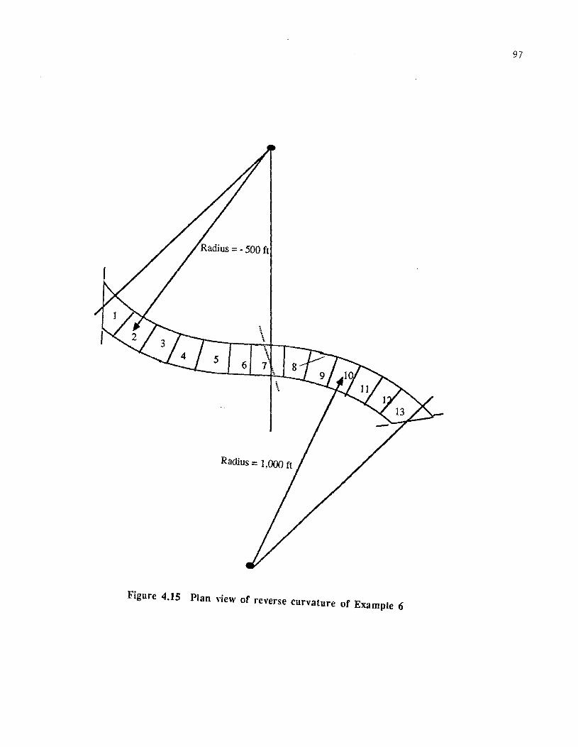
97
Radius = 1,000 ft
Figure 4.15 Plan "jew of reverse curvature of Example 6

98
computer programs. It may be best to approximate designs with the V-load method and fmalize the design
with this program. The other part of this research project was to automate the V-load design on a personal
computer. A data me for the finite element solution can be directly taken from the data required for the V
load program. In this way. the data preparation need only be done once. A comparison of the accuracy of the
V-load method for different bridge parameters is given in Chapter 5.

CHAPTER S. PARAMETER STUDY AND PROGRAM VERIFICATION
5.1 INTRODUCTION
This chapter compares two bridge geometries with changing parameters to the V-load method. This
was done to verify that each program worked for these geometries and to study the behavior of curved bridges
with different parameters. In this way, the range of parameters could be established for the V-load method for
acceptable error. Also this chapter uses a third bridge to verify the accuracy of the finite element analysis
with two other finite element programs.
The three bridges studied were:
1) The bridge of example 1 in Chapter 4. The radius was changed from 500 feet to 1,000 feet for
both the dead load and truck load cases. The diaphragm spacing also changed from 10 to 20 feet
for each radius.
2) A three-span curved bridge with a 32.7-degree curve. The four-girder bridge plans were supplied
by the Texas Highway Department and represent an actual design. Three radii, different
diaphragm spacings, and radial and skewed supports were used to study different bridge
parameters in a comparison with the V -load method. Both dead load and truck loads were used
on some of the parameter studies.
3) The bridge of example 2 in Chapter 4. The three-span bridge plans were also supplied by the
Texas Highway department. In this case, two finite element solutions were available for
comparison and the program could be better verified.
5.2 PARAMETER STUDY ON A SIMPLE SPAN CURVED BRIDGE
This bridge was termed scheme A and was chosen because of its simplicity in geometry. With the
simple geometry, curved bridge behavior could be more easily understood. The bridge was also a good
validation of both the V -load and the finite element programs in that the radius could be increased to a large
value and the results could be comput'ed by hand since the bridge is statically determinate. The spacing of the
girders was chosen to coincide with the wheels of the truck so that distribution factors would not be involved
when comparing the V-load and the finite element results.
The results of the parameter study are shown in Table 5.1. The table shows that two radii of 500 and
1,000 feet with two diaphragm spacings of 10 and 20 feet were used as a simple parameter study on the 100-
foot bridge. The values studied were the maximum stress due to dead load, worst case live load, and total
load. Also, the warping stresses were determined for the dead load and total load case.
The table shows that as the radius decreased, more of the load was transfered from the inner to the
outer girder for a given diaphragm spacing. This transfer of load was independent of the diaphragm spacing.
The transfer of load from the inner to outer girder was much less evident for the composite girder in the live
load case. The live load case was different because the slab provided torsional stiffness and this stiffness
dominated over the steel girder stiffness.
The radius change also had a big influence on the warping stresses. When the radius was halved, the
warping stresses almost doubled. Also, when the diaphragm spacing was doubled, the warping stresses almost
doubled. The function of the diaphragms was to brace the girders and to make the bridge torsionally stiffer. As
the load transfer was increased from the inner to outer girder due to a decrease in radius, the diaphragms had
99
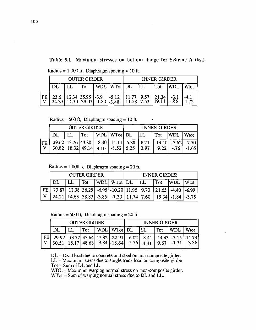
100
Table 5.1 Maximum stresses on bottom flange for Scheme A (ksi)
Radius = 1,000 ft, Diaphragm spacing = 10ft
OUTER GIRDER INNER GIRDER
DL LL Tot WDL WTot DL LL Tot WDL Wtot
FE 23.6 12.34 35.95 -3.9 -5.12 11.77 9.57 21.34 -4.1 V 24.37 14.70 39.07 -1.80 -3.48 11.58 7.53 19.11 -ll -. 8 -1.72
Radius = 500 ft, Diaphragm spacing = 10 ft
OUTER GIRDER INNER GIRDER
DL LL Tot WDL WTot DL LL Tot WDL
FE 29.62 13.76 43.88 -8.40 -11.11 5.88 8.21 14.10 -5.62 V 30.82 18.32 49.14 -4.10 -8.52 5.25 3.97 9.22 -.76
Radius = 1,000 ft, Diaphragm spacing = 20 ft
FE V
FE V
OUTER GIRDER INNER GIRDER
DL LL Tot WDL WTot DL LL Tot WDL
23.87 12.38 36.25 -6.95 -10.20 11.95 9.70 21.65 -4.40 24.21 14.63 38.83 -3.85 -7.39 11.74 7.60 19.34 -1.84
Radius = 500 ft, Diaphragm spacing = 20 ft
OUTER GIRDER INNER GIRDER
DL LL Tot WDL WTot DL LL Tot WDL
29.92 13.72 43.64 15.82 -22.91 6.02 8.41 14.43 -7.15 30.51 18.17 48.68 -9.84 -18.64 5.56 4.41 9.67 -1.71
DL = Dead load due to concrete and steel on non-composite girder. LL = Maximum stress due to single truck load on composite girder. Tot = Sum ofDL and LL WDL = Maximum warping normal stress on non-composite girder. WTot = Sum of warping normal stress due to DL and LL.
Wtot
-7.50 -1.65
Wtot
-6.99
-3.75
Wtot
-11.73 -3.86

101
to transfer more of this load. Many things affect warping stresses and this example showed that the stresses
can be significant.
The V-load compared well against the finite element solution for bending stressses, especially in the
dead load noncomposite case. The dead load bending stresses were predicted with an error of less than 4%.
The live load error was around 18% for the l.000-foot radius and 32% for the 500-foot radius. The total error
for the total stress was stil11ess than 10%. The reason the live load error was so high was the fact that the V
load method did not take into account the torsional slab stiffness in its model. The V -load transferred too
much load to the outer girder in the composite case. This was not a conservative model since the equal load
was taken off the inner girder. The outer girder would end up being overconservative and the inner girder
would be unconservative.
The warping stresses did not compare too well between the two solutions. The place of maximum
stress did not agree either. The finite element gave maximum stresses between diaphragms while the V -load
gave maximum stresses at diaphragm locations. The V -load assumed the diaphragms provided a rigid support
so the maximum moment would most likely occur at that point. The fmite element solution probably gave
higher numbers because the diaphragms did not act in such a rigid manner for this simply-supported, two-girder
case.
A few other things may have accounted for the discrepancy between the V-load and the finite element
solution. The results of the fmite element were given as an axial stress for the flange and warping stresses at
the flange nodes. The bending stress could be thought of as an average stress for the member. For positive
moments, as in this example, this was not bad since the gradient was very low but for continuous spans the
program would most likely not give the true peak negative moment stress because of the steep gradienL The
warping stresses also had a steep gradient at the diaphragms but the finite element solution, like the V -load,
gave the warping stresses at node locations. The V-load used more increments along the span to determine
both the bending stresses and the warping stresses compared to the fmite element model. A difference in
results can be attributed to the difference in the refinement of the fmite element mesh and the increments of
the V-load.
5.3 PARAMETER STUDY ON A THREE-SPAN CURVED BRIDGE
The bridge for scheme B is shown in Figure 5.1 and was taken from plans supplied by the Texas
Highway DepartmenL A few simplifications were made to more easily model the bridge. First, the overhang
was increased so that each girder would have the same amount of concrete on each side. Also the same
flange sizes were used for each girder and the flange sizes in the positve moment region were made the same
for each span. Most of the same things studied for scheme A were studied in scheme B. The maximum positive and
negative bending and warping stresses were determined for both the V -load and the fmite element solutions.
Case I, Case 2, and Case 3 were used to swdy the effect of diaphragm spacing on the maximum stresses.
Case I, Case 4, and Case 5 were used to swdy the effect of the radius on the maximum stresses. Case 6 and
Case 7 are shown in Figures 5.2 and 5.3 and were used to study the effect of skew on the maximum stresses.
Also, the effect of live load on different radii bridges were used in Cases 1 and 4.
Table 5.2 shows the results in the swdy of the effect of the radius on the maximum bending stress.
The first thing that is evident is that the stresses are low. Perhaps the bridge design was conservative and the
simplifying assumptions made it more so. The maximum stress did not change much when the radius doubled

102
I 1.0 x 16.0
40 x 0.3125
. 1.5 x 16.0
Girder sizes for
16 17
10 bays
8 bays
R = 175 ft Selia = 10.46 ft
7.33' ... ~ 3.
----I ~l~'" R = 175 ft 1.3 •
I 2.5 x 16.0
40 x 0.3125
2.5 x 16.0
subst. 1-6,11-16,21-26 Girder sizes for subst. 7-10,17-20
Figure 5.1 Case 1 of scheme B.
8"

I \ 10 bays - 4 deg skew
30 deg skew 8 bays
R= 175ft Sdia = 10.46 ft except for substructures 8 and 17 with Sdia = 20.92 ft
Figure 5.2 Case 6 of scheme B.
103

104
\27 deg skew
\ 10 bays -17 de! skew 17 deg skew 8 bays
-27 deg skew I
R=175ft Sdia = 10.46 ft except for substructures 8 and 17 with Sdia = 20.92 ft
Figure 5.3 Case 7 of scheme B.

Table 5.2 Maximum bending stresses at the centerline of the bottom flange for Scheme B (ksi).
Case 1 Radius = 175ft, Diaphragm spacing = 10.4615 ft
Girder 1 Girder 2 Girder 3 Girder 4
Load Max Case Mom V-load Fern V-load Fern V-Ioac Fern V-load Fern
DL POSe 7.27 6.52 5.56 5.24 4.03 3.90 2.61 2.31 Neg. -8.72 -7.47 -7.57 -6.90 -6.50 -6.12 -5.49 -5.29
LL1 POSe 5.88 3.70 1.17 -1.46 L12 POSe 3.32 2.84 2.02 0.88
Case 4 Radius = 350 ft, Diaphragm spacing = 10.4615 ft
Girder 1 Girder 2 Girder 3 Girder 4
Load Max Case Mom V-load Fern V-load Fern V-Ioac Fern V-load Fern
DL POSe 5.81 5.57 5.03 4.88 4.29 4.20 3.58 3.45 Neg. -7.64 -6.65 -7.10 -6.36 -6.57 -5.88 -6.06 -5.47
LL1 POSe 5.29 3.37 1.30 -0.79 LL2 POSe
2.78 2.58 2.17 1.55
Case 5 Radius = 700 ft, Diaphragm spacing = 10.4615 ft
Girder 1 Girder 2 Girder 3 Girder 4
Load Max Case Mom V-load Fern V-load Fern V-Ioac Fern V-load Fern
DL POSe 5.15 5.07 4.77 4.71 4.40 4.36 4.05 4.00 Neg. -7.13 -6.36 -6.87 -6.14 -6.61 -5.98 -6.35 -5.78
LL1 = One truck loaded for maximum positive moment over girders 1 and 2. LL2 = One truck loaded for maximum positive moment over girders 2 and 3.
105

106
from 175 to 350 feet, but there was a slight decrease when the radius increased from 350 to 700 feet. The V
load compared quite well for the dead load positive stress and a little worse for the dead load negative stress.
The percent difference was always less than 10% for the dead load. however.
As stated in Section 5.2, the nonnal bending stresses for the flange were average stresses. Since the
negative moment gradient at the support was steep, the true peak stress was most likely missed by the finite
element due to averaging. The maximum stresses given in Table 5.2 represent extrapOlations of the plot of
bending stresses along the span. The difference between the stress printed out and the peak stress at the
support in these cases varied up to 5%. The user is cautioned that the axial stresses printed out by the program
should be considered as stresses at the midpoint between nodes.
Two live loads were run for both Case 1 and Case 4. The V -load marched a truck across the bridge
and determined the worst longibJdinal load position for positive momenl The wheel spacing of the bUCk was
chosen to be direcdy over the girders so that the V -load program could bener determine the proper distribution
factors. The truck was then placed over girders I and 2 for one load case and over 2 and 3 for the other load
case. The results are shown in Table 5.2. The load placed on the outer two girders produced the maximum
stresses and torsion in the bridge. This load case also caused a negative moment in girder I. The bUCk over
the middle girders controlled for the ,inner girders. Also, the doubling of the radius caused a slight decrease in
the bending stresses for the outer girder. The change in stress with the increase in radii was less in the live
load case than the dead load case because the slab provided so much stiffness. This live load study showed
that the truck needs to be moved around a lot to get the worst case for each girder. Also, depending on the
truck placement, the stress range on the girders can change and this is important in fatigue design. The V-load
can help in this placement but it has distribtion factors built in the program which mayor may not help give
the worst load case.
Table 5.3 shows the results of the effect of different diaphragm spacings on the warping stresses. As
can be expected, the largest warping stresses occured when the diaphragm spacing was the largesl A
dramatic decrease occurred when the diaphragm spacing was cut in half from 20.92 feet to 10.46 feet. A
further decrease in warping stresses occurred when the diaphragm spacing was decreased to 6.97 feel It was
evident that there was a diminishing point of returns for decreasing the diaphragm spacing.
Table 5.3 shows that the V -load was quite good for detennining the warping stresses when compared
to the fmite element solutions. It can also be noted that the warping stresses were only significant for a
diaphragm spacing of 20.92 feel This large diaphragm spacing probably exceeded what most designers would
recommend and it was double the designed spacing in this case. The V-load agreed bener for the continuous
case perhaps because the four girders and the continuous spans forced the diaphragms to act in a more rigid
manner.
A plot of the finite element warping stresses along half the span for girders one and four is shown in
Figure 5.4. The three lines on each plot represent the three diaphragm spacings studied. A couple of things
are evident from the plot. First, the dramatic difference in warping stresses for each diaphragm spacing is
evident. The 2O.92-foot diaphragm spacing dominates in relation to the other diaphragm spacings. The
diaphragm serves as a reaction point for the flange as shown in Figures 1.2. 1.4 and 1.5b. When there is a
positive bending moment as in Figure 1.4, the axial stresses in the flange are not collinear and the flange is
supported by the diaphragm. Tension stresses were developed on the OUler point of the flanges when the
moment was positive. This is shown in Figure 5.4 which a positive sign represents a tension on the outer fiber
of the flange. The plot resembles a continuous span with supports at diaphragm locations. The first interior
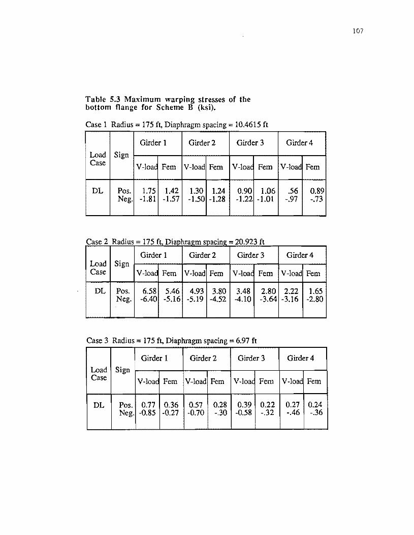
Table 5.3 Maximum warping stresses of the bottom flange for Scheme B (ksi).
Case 1 Radius = 175 ft, Diaphragm spacing = 10.4615 ft
Girder 1 Girder 2 Girder 3
Load Sign Case V-load Fern V-load Fern V-Ioac Fern
DL Pos. 1.75 1.42 1.30 1.24 0.90 1.06 Neg. -1.81 -1.57 -1.50 -1.28 -1.22 -1.01
C 2 Rd' ase a IUS = 175 f D' h 0923f :t, lap] ra,;m spacmg = 2 . t
Girder 1 Girder 2 Girder 3 Load Sign Case V-load Fern V-load Fern V-Ioac Fern
DL Pos. 6.58 5.46 4.93 3.80 3.48 2.80 Neg. -6.40 -5.16 -5.19 -4.52 -4.10 -3.64
Case 3 Radius = 175 ft. Diaphragm spacing == 6.97 ft
Girder 1 Girder 2 Girder 3
Load Sign Case V-load Fern V-load Fern V-Ioac Fem
DL Pos. 0.77 0.36 0.57 0.28 0.39 0.22 Neg. -0.85 -0.27 -0.70 -.30 -0.58 -.32
107
Girder 4
V-load Fern
.56 0.89 -.97 -.73
Girder 4
V-load Fern
2.22 1.65 -3.16 -2.80
Girder 4
V-load Fern
0.27 0.24 -.46 -.36

108
• Or;) .:..c:: •
Warping Stress Along Span Casel,2,3 for G 1 6
-6;-~~-r--~~---r--~~~-r--~~
Oe+O 1 e-l 2e-l 3e-1
Distance xii 4e-l 5e-1
III Case3Gl • Case2Gl a CaselGl
Warping Stress Along Span Casel,2,3 for G4 2
-3~--~-r--~~---r--~~~-r--~~
Oe+O 1 e-l
Figure 5.4
2e-l 3e-l
Distance xii 4e-l 5e-1
III Case1G4 • Case2G4 a Case3G4

109
suppon is near 0.31 and the stress in the outer fiber goes in compression in the negative moment region. 1be
plot for the inner girder looks much like the one for the outer girder except the warping stresses are smaller.
This is most likely due to the load transfer to the outer girder due to the curvature.
Plots of the stresses for girder I and 4 of case 6 and case 7 along half the span is shown in Figure 5.5.
The plots show how dramatic a difference the skewed supports make. The top graph penains to the bridge in
Figure 5.2. The positive moment for the outer girder was greater than inner girder in the extmor span and less
in the interior span. The maximum stress for the inner girder of the interior span could be attributed to the
sharp curvature of the bridge. Both plots showed a local stress variation near the inflection point of the other
girder. The infection point of girder one would require no load transfer to the outer girder since the flange
forces are balanced. This was the reason that there was a slight increase in stress in girder 4 when girder I
was at its inflection poinL With radial supports, these inflection points would line up transversely and this
local maximum would not be as evidenL The warping stresses for the skewed supports were pretty bigb near
the skewed supports but dropped off to low levels away from the sUPPOrL This is understandable since this
model had the diaphragms farther apan due to the curvature. Also, diaphragms were not placed over the
suppon so that the diaphragms would only be radial. Consequently, the unsupponed length of the warping of
the flange doubled and the warping stresses increased sharply. A different modeling of the diaphragms at the
skewed support would change the warping stresses.
5.4 KURV87 COMPARISON WITH TWO OTHER MODELS
Because the V -load method was an approximate method, a more stringent comparison of the finite
element was needed. The Texas Depanment of Transponaton had determined a typical bridge to analyze and
it represents Example 2 in Chapter 4.
The bridge division used the Shell 8 program to develop two finite element models to analyze the
bridge. The first model used plate elements to model the flange, slab and web elements. This model was
deemed to be not too reliable since the aspect ratio for the flange elements was over 20. The second model
used beam elements for the flanges in much the same way as Kurv87 did. The difference between these two
models was the slab placemenL The slab was placed at the same location as the flange in the bridge division
model while Kurv87 used rigid links as shear studs and placed the concrete slab physically away from the top
flange. This difference should not have been impottant for the dead load noncomposite case since the slab was only supplying load and no stiffness.
In the course of the model comparison it was decided to look at the effect of the bottom 1ateral braces.
The bridge division ran its truss model with and without the bottom bracing as did the Kurv87 program. As
stated in Chapter 4, the bridge division's truss model used braces that switched back and forth in every bay.
For easier modeling, Kurv87 used X-bracing in each bay with half the area so that the dead load was the same
and the stiffness was about the same. 1be plate model was not run without the braces.
The results of the study are shown in Table 5.4. The maximum deflection predicted by the Kurv87
program fell in the middle of the two maximum deflections predicted by the truss and plate models. An
average percent difference for the Kurv87 program and the truss model was about 1.8% for the exterior span.
An average percent difference for the Kurv87 program and the plate model was about -2.7%. The Kurv87
program predicted a little less rotation than the other two models in exterior span. The deflections predicted
by the Kurv87 program in the interior span was greater than the other two models. The numbers were still
relatively close, however.

110
• .• III
.:0.: • ~ ... -00 ell I: .• "C I: <lJ
CQ
10
0
Bending Stress Along Span, Case6, Gl,G4
III Case6-G4 • Case6-G1
-10~--r-~--~--r-~--'-~r--r--'-~
Oe+O
6
• 4 'I;; .:0.: • ~ 2 -00 0 ell I: ~ -2 c <lJ
CQ -4
1 e-1 2e-1 3e-1
Distance x/J 4e-1 5e-1
Bending Stress Along Span, Case7, Gl,G4
III Case7-G1 • Case7-G4
-6~~--r-~-.--~.-~--~'--'--~
-1e-1 1e-20 1e-1 2e-1 3e-1 4e-1 5e-1
Distance x/l
Fi gure 5.5
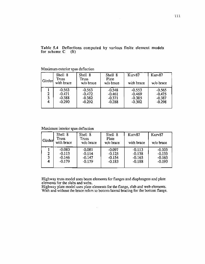
Table 5.4 Deflections computed by various finite element models for scheme C (ft)
Maximum exterior span deflection
Shell 8 Shell 8 Shell 8 Kurv87 Kurv87
Girder Truss Truss Plate with brace w/o brace w/o brace with brace w/o brace
1 -0.563 -0.563 -0.548 -0.553 -0.565 2 -0.471 -0.472 -0.461 -0.469 -0.475 3 -0.388 -0.382 -0.371 -0.385 -0.387 4 -0.290 -0.292 -0.288 -0.302 -0.298
Maximum interior span deflection
Shell 8 Shell 8 Shell 8 Kurv87 Kurv87
Girder Truss Truss Plate with brace w/o brace w/o brace with brace w/o brace
..
1 -0.080 -0.081 -0.097 -0.113 -0.103 2 -0.113 -0.114 -0.125 -0.138 -0.133 3 -0.146 -0.147 -0.154 -0.163 -0.163 4 -0.179 -0.179 -0.183 -0.188 -0.193
Highway truss model uses beam elements for flanges and diaphragms and plate elements for the slabs and webs. Highway plate model uses plate elements for the flange, slab and web elements. With and without the brace refers to bottom lateral bracing for the bottom flange.
111

112
The bracing had little influence on the deflection of the members. The brace seemed to stiffen up the
bridge torsionally because the rotation was slightly less. The difference in modeling the X-bracing did DOt
seem to represent a problem except that the deflections between the two models were slightly closer without
the brace than with the brace. The effect of the bracing probably did not show up 100 much since the 5-degree
curvature was pretty low. The bottom lateral bracing most likely would have a much larger effect for a sharper
curved bridge.
55 SUMMARY The effect of diaphragm spacing, radius, skew, and loading was studied for both bending and warping
stresses. The following conclusions can be drawn:
1) When the radius decreased, the warping stress and the load transfer to the outer girder increased.
2) When the diaphragm spacings increased, the warping stresses increased.
3) The V -load was very good for predicting dead load stresses but it was not nearly as good at
predicting live load stresses since it ignored the contribution of the slab stiffness. The error for the
sum of the dead load and live load stresses was still less than 10%, however.
4) The V-load predicted warping stresses better for the four-girder, three-span bridge than for the two
girder simple span bridge.
5) It is difficult to make general statements on the skewed bridges except for some obvious
statements. The maximum bending stresses near the skewed suppon did not occur at the same
distance away from the suppon or even on the same relative side of the support The warping
stresses in this model were much larger near the suppon due to a larger diaphragm spacing.
6) The Kurv87 program will give the proper peak stresses for the positive moment region but it will
not give the true peak stress at a support The user must extrapolate the correct stress at the
suppon or run a fme mesh for a final design check.
7) The Kurv87 program compared extremely well with two other finite element models and the user
can be confident in the results obtained.
8) The effect of the bottom lateral bracing was not seen to be 100 significant in the bridge studied
even though a little less rotation was evidenL The influence of the bottom bracing most likely
will be more evident for more sharply curved bridges.
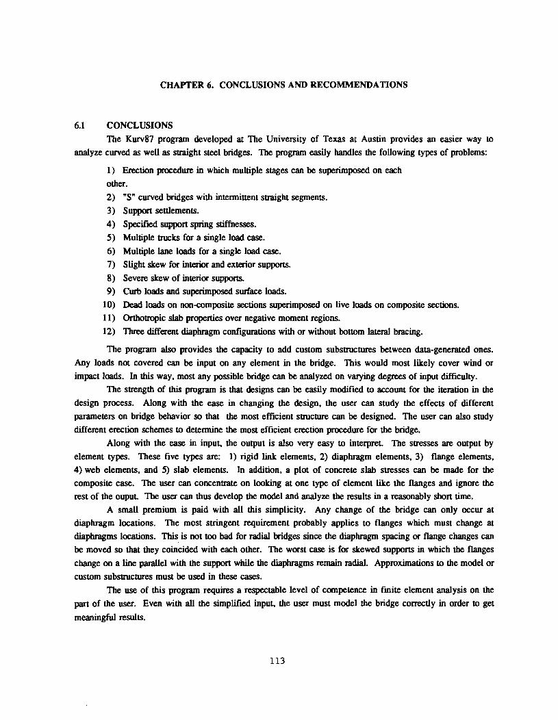
CHAPTER 6. CONCLUSIONS AND RECOMMENDATIONS
6.1 CONCLUSIONS
The Kurv87 program developed at The University of Texas at Austin provides an easier way to
analyze curved as well as straight steel bridges. The program easily handles the following types of problems:
1) Erection procedure in which multiple stages can be superimposed on each
other.
2) "S" curved bridges with intennittent straight segments.
3) Support settlements.
4) Specified suppon spring stiffnesses.
5) Multiple trucks for a single load case.
6) Multiple lane loads for a single load case.
7) Slight skew for interior and exterior suppons.
8) Severe skew of interior supports.
9) Curb loads and superimposed surface loads.
10) Dead loads on non-composite sections superimposed on live loads on composite sections.
11) Orthob'Opic slab properties over negative moment regions.
12) Three different diaphragm configurations with or without bottom lateral bracing.
The program also provides the capacity to add custom substructures between data-generated ones.
Any loads not covered can be input on any element in the bridge. This would most likely cover wind or
impact loads. In this way. most any possible bridge can be analyzed on varying degrees of input difficulty.
The strength of this program is that designs can be easily modified to account for the iteration in the
design process. Along with the ease in changing the design. the user can study the effects of different
parameters on bridge behavior so that the most efficient structure can be designed. The user can also study
different erection schemes to detennine the most efficient erection procedure for the bridge.
Along with the ease in input, the output is also very easy to interpret. The stresses are output by
element types. These five types are: 1) rigid link elements. 2) diaphragm elements. 3) flange elements.
4) web elements. and 5) slab elements. In addition. a plot of concrete slab stresses can be made for the
composite case. The user can concentrate on looking at one type of element like the flanges and ignore the
rest of the oupuL The user can thus develop the model and analyze the results in a reasonably shon time.
A small premium is paid with all this simplicity. Any change of the bridge can only occur at
diaphragm locations. The most stringent requirement probably applies to flanges which must change at
diaphragms locations. This is not too bad for radial bridges since the diaphragm spacing or flange changes can
be moved so that they coincided with each other. The worst case is for skewed supports in which the flanges
change on a line parallel with the suppon while the diaphragms remain radial. Approximations to the model or
custom substructures must be used in these cases.
The use of this program requires a respectable level of competence in fmite element analysis on the
part of the user. Even with all the simplified input, the user must model the bridge correctly in order to get
meaningful results.
113

114
62 RECOMMENDATIONS FOR FUTURE RESEARCH
Further research in the area of bridge analysis could involve modifying the Kurv87 program or
developing a more powerful analysis tool. The following are recommendations on further research into bridge
analysis programs:
1) Modify the data generator to generate both steel I-girder and steel box girder geometries.
2) Modify the data generator to generate a triangular substructure for severely skewed end supports.
3) Modify the data generator so the actual flange locations as opposed to the average flange
thicknesses can be used in the vertical placement of the nodes.
4) Modify the data generator so that the girder depth does not have to be constant over the bridge.
This most likely would be needed for the negative moment regions of straight bridges.
5) Enhance the program so that pinned connections can be used between girders. This would be
useful in analyzing the erection stages.
6) Enhance the program to be able to handle multiple load cases.
7) Adapt a graphics package so that the input could be taken directly from another data me
representing a description of the bridge.
A good foundation has been laid for further enhancements to this progam so that many aspects of
bridge design can be easily and efficiently accomplished.

APPENDIX A
CHANGING THE COMPUTER PROGRAM
115

116
Listed in the following table are size limitaions which can be changed so that different sized problems
can be solved.
LIMITATION
12 Wheels
10 Spans
10 Girders
Max. No. of divisions
between diapbr = 8
No. of Elements = 200
Maximum number of
substructures = 16
Number of Nodes
(max number = 162)
V ARIABLES TO CHANGE
Centtr(12), Cent1g(12), Trld
Nsubbc(lO)
S g ir( 1 0) ,Masin (7 0)
Dthet(8)
Itp(200),Kbeam(200),P
Poc(24,16,200)
Poc(24, 16,200),Pr(24, 16)
X(450,16),
Szq(3,200,16),Sgq(3,200, 16)
Xq(l62), Yq( 162),Zq(l62)
R(l62), Angle(l62)
SUBROUTINE OR
COMMON BLOCK
Readtr in Genpuz
Common lPuz/
Trdelt, Lanld and Truck
in Genpuz
Common in Recpuz
Loads,Gensol, Unit2 in
in Genpuz
Loads, Gensol, Unit2
Common in Puzf83
Common /dum! in
Recpuz
Common in Genpuz
To change the plate girder to include a box girder the following changes need to be made:
1) Change node locations in subroutine NODGEN.
2) Change element generator and element node numbering in subroutine
ELNOD.
3) Make sure variables NXND, NXB and NXT give correct values.
To change the graphics the folliwing subroutines need to be changed:
1) Subroutine PLOTSG in Genpuz which calls subroutines PLOTXY and
PLOTYZ.
2) Subroutine PLOTSL in Recpuz.

APPENDIX n COMPUTER PROGRAM LISTING OF INPUT
FILES FOR EXAMPLES IN CHAPTER 4
117
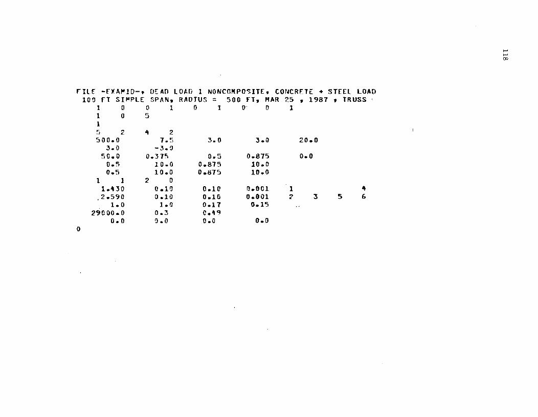
rILE -FXA~lD-, DEAD LOAD 1 NONCO~POSIT[, CONCRfTE + STEEL LOAD
0
100 rT SI~PLE SPAN, RADIUS = 500 fT, MAR 25 , 1981 , TRUSS 1 0 0 1 0 1 00 1 105 1 '5 ... It 2 .:: 500.0 7.5 3.0 3.0
3.0 -3.3 5~.O 0.375 0.5 0.875
0.5 10.0 0.875 10.0 0.5 10.0 0.875 10.0
1 1 2 0 1." J 0 0.10 0.10 0.001 1
.2.590 0.10 O.Hi 0.001 -; 1.0 1.1) 0.17 0.15
29COO.0 0.3 c .... ~ 0.0 (J.O 0.0 0.11
20.0
0.0
3 5 " 6
,..... ,..... co

FILE -EXAHIT-, THIS JS 130 fOOT SIMPL[ SPAN,
1 002 1 0 ~
1 5 2 4 2 500.0 1.5
3.0 -3.0 50.0 0.375
O.s 10.0 0.5 10.0
1 1 2 0 1.430 0.10 2.590 0.10
3625.0 3625.0 29000.0 0.3
0.0 D.O 1
HS 20-'14 0 1.0 6
~.o 3.00 li.O -3.C 0
1(,.0 3.00 16.0 -3.D£) H .. G 3.00 1(uO -3.0u
\}
A T~ST CASE fOR TRUCK LOADING, TRUSS RADIUS = 500 FOOT, APR 13, 1987 o 1 !) 0 0
3.0 3.0 20.0
0.5 0.875 0.0 0.B75 10.0 0.815 10.0
0.10 0.001 1 0.10 0.001 2 3 5 0.15 0.00 0.00 0.0 1.0
5~. n 0.0 500.0 FOR."
14.00 1'1.00
0.0 0.0
-l~.OO
-14.00
4 6
I-' I-' ~

I-'OUSTO~ I'RIOG£' DIVISION. 4t GIRDER BRIl)GE FRO" "R. EO SUCHICKI. 3 SPAN. 1~4.71 rT, 215.5 ~T, 18~.71 fT~ 5 DEG CURVE. OLI NON-CO"POSITE
11 0 1 'l " 0 0 0 1 3 12 12 !If 12 1 :3 1 1 At
l1i15.91":1(, e.o 3.0 3.0 15.392~
12.0 "'.0 -4.0 -12.0 72.0 0.5625 0.0 o .D 0.0
1.0 lR.O 1.5 1~ .0 1 .. 0 IR.G 1.5 1R.0 1.0 10.0 I.'} 18.0 1.0 18.0 1.5 18.0
1 I 1 " 1.525 0.01 O.'ll 0.001 1 2 3 ~ 5 b 1.<\05 il.01 0.01 0.001
1 2 ., 1 • :3 1\ It '3
1.0 1.0 0.17 0.15 2<;1000.0 0.3 0.-9
0.0 0.1) 0.0 0.0 , oJ
.... (
..... c 1 4
10 0 1.0 18.0 2.0 18.D 1.0 16.0 2.0 18.0
I-' N o

1.0 1.0
(I ... '-
? 1 :.'I
10 0 1.0 1.0 1.0 1.0
~
" . :' 1 ~
1':.1 0 3.0 3.0 3.0 3.0
0 '> { . .,
3 10 0
l.e 1.0 1.0 1.0
0
18.0 2.0 18.0 2.0
18.0 1.5 IR.O 1.5 18.0 1.5 18.0 1.5
lR.O 3.0 l~ .0 3.0 18.0 :5.0 18.0 3.0
tH.O 1.~
18.0 1.5 18.0 1.5 18.0 1.5
18.0 18.0
18.0 18.0 lR.O 18.0
18.0 ·18.0 18.0 18.0
18.0 19.0 18.0 18.0
t-' N t-'

t-' N N
2 ?
1 4 10 0
1.0 18.0 2.0 18.0 1.0 18.0 2.0 IIJ.O 1.0 18.0 2.0 18.0 1.0 lR.O 2.0 18.0
0 ~
? 1 :5
10 0 1.0 18.0 1.5 18.0 1.0 18.0 1.5 18.0 1.0 18.e 1.5 18.0 1.0 18.0 1.5 18.0
~
2 ., "-
I Al 10 0
1.0 lR.O 3.0 IR.D 3.0 18.0 3.0 18.0 3.0 18.0 3.0 lR .0 3.0 !8.0 3.0 18.0
'J :2 2 1 3
1~ 0

1.0 1.0 1.0 1.0
~ ., .: , I ,.
10 0 1.0 1.0 1.0 1.1)
0 ,.., <
? 1 :3
10 0 1.G I.e 1.v 1.0
18.0 1.5 18.0 1.5 18.0 1.5 18.0 1.5
lR.(I 2.0 IR.D 2.0 18.0 2.0 !fl.O 2.0
IR.D 1.5 18.0 1.r; IP.O 1.~
lR .0 1.5
18.0 18.0 18.0 1~.O
18.0 18.0 18.0 18.0
If1.D 18.0 18.0 18.0
t-' N W

EXAMPLE 3. 2 SPAN. 3 S[VER[ SKE~ INTERIOR
5 0 1 0 ? 776 o '3 1.0(+31) o 3 2.0[+3J o :5 3.0r+30 7 3 3.0[+31) 7 '3 2 .. 0E+30 7 :5 1.·0~+30
13 3 1.0E+30 13 3 2.0[+30 13 3 3.J~+30
1 5 1 :? ~
0.0 7 .. ,:, 8.8333 Q ./)
60.0 O.l\ 375 0.5625 16.0 0.5E.25 16.0 O.!l6?5 16.0 2 2 2 0 1.430 !l.lO 2.590 0.10
1.0 1.0 29000.00 0.3
0.0 0.0 0
GIRDERS, orAD LOAD ONLY. NON-CO"POSITE SUPPORT, SPRING STIFFNESSES ARE SPECIFIED
o 090 1
3 .. 0 3.0 16.0 -8.8333
0.80 1.0 0.0 1. a 16.0 1.0 Hun 1.0 16.0
0.10 0.001 1 " 0.10 0.001 '3 £. 0.11 0.15 0.'49 0.0 0.0
...... N .P-

2 .., <-
I 1 10 0 0.5625 Hi.O 1.00 16.0 0.5625 16.(' 1.00 16.0
1.00 16.0 1.25 16.0 !'
14-.., <-
I ~
J.
10 C 1.00 16.0 1.25 16.1) 1.00 1£..0 1.25 16.0 1.00 1G.O 1.25 16.0
:5 1 0
2 2 1 1
10 0 1.00 16.0 1.25 16.0
0.5625 16.1) 1.0 16.0 0.5625 16.0 1.0 16.0
0 ? 2 1 5
10 0 0.5625 16.0 1.0 16.0 0.5625 16.0 1.0 16.0 0.'5625 16.0 1.0 16.0
0
t-' N V1

126
wo ... w ~,...
enUo e ... o.u EW 00.. UCI.I I Zw Oct ZC
·W )00"'" ..Jw zcn Q I .. n:;)
Z QUo cue .... ..J ... ...,
CIl Q CU) wz O ... r:,
tit .Q..
V) V) ~ LJ .. 0 0(1) ac: ... ... ~ 1110
0. P"'ICI. .. =:.
I'!:IU'loc.;.Q
""1"')"" ... ... ... 2' In C 0.. .J r,i ~ cII.J
"' • 1.1
'fI':.c CIl
w ..J 1.1.1 0. a: a::1.4J 'II/l.:iII lOI: l.Ll WV:
0 "-
co (,
ht hl • t Q c;, .....
t • • I<"'l !'. .....
... ... ,..
.... ..... ....
o
.... , ~ .-' .. ..... ...... ..-j
'" .,.. '-. . - "' -. ./' .... .~
-. .,.. .,.... cr. ~ .-. .:'1 ... I!' ... -• CJ ( . I r . a, ~, ,., .... y-
..-4 -
,..,
J • ...., ..-I ....
<r eo , ... "j
...;
!'J 11"\ 1..0 .....
;... U'I ~ ..-( ~ ....
I;, ..c ~

n ?J rl 21 Q '~? .. -
H ?3 20 13 10 ~~ 21 !\ 11 ?:l .~? 9 14 n 10 2~
11 :"'~
! ~ 11 9 1 J
10 11 2C :I.e, 23 2; .... 1 .... < ~ • ::>
:'4 ., . _::>
~. ,~ '" ?l ~' I 211 ~~ 1 . , U ~:, ;' 1 ;.~ ... 2:' IE. ?(]
11 2l lA ?:!
i -21.'~~ -11.633 '? -It;. 000 -B.U33 J -U'.!) -8.833 .. -1(,.0 -~.f.~3
') 0.0 G.O £, n.J -B.833
5.~20B33 1.0 0.0 5.420833 1.0 0.0 5.015. 1.0 0.0 1.0 1.!) 0.0 S.,.20P.33 1.0 0.0 5.420e33 1.0 O.C
G.I) 0.0 1.0 0.0 0.0 1.0 0.0 0.0 1.G 0.0 !J.O 1.0 0.0 0.0 1.0 0.0 [J.O 1.0
0.0 0.0
10.0 0.0 c.o 0.0
t-' N '-J

7 f.l -11.f\33 ~.o\?OB33 .: (;.0 0.0 3.075 L
" n.J -!:i.e33 ~ .. O75 }:J G.~ 0.0 0.0 11 O.G -8.Al3 0.0 !? If,.!} !:\ .tnJ 5.4?IJR33 1 ,~ 1 f,. :J tJ.Jil3 5.01':.t l'I I (Je :) H.tnJ 0.0 1'J ;';1."~' 11.!H3 5.\20£133
I" 21.~J~ 9.u31 ~."20a33 17 ?:1."~~ 0.0 :'.420833 13 21.IfH -R. ~IJ 3 5.\20B33 1<J 21.4!~ -ll.tfB 5.420833 2;J ~l.L\H B.tBJ 5.075 ?l 2! .4H 0.0 5.075 '> , L ~ 2!.L\H -~.~33 5.015 " . 21.4314 R .IU3 :l.0 c ~:
~'IJ 21.q:H lI.O n.o ~. :; 2].'1H -~.113~ ~.O ., , , ., ='l.ql~ ~ .}:, 1 2.5375 ."f :'1.4"" -'\.1507 ?~~75
ry rl 29(:100.0 2.!:l60 ,-... () 2:1000.0 ?RF.O 'I () 2JOOO.il 5.180 ~ 0 2jilJu.J :?.~&O
~' 0 2~:::;OO.O 2.860 " 0 2 r, i) 0 (1 • tl 5 .. 180 '--
1.0 0.0 0.0 D.O 1.0 0.0 0.0 tI.O 1.0 0.0 0.0 1).0 1.0 0.0 0.0 0.0 1.0 0.0 Il.D l.O 1.0 0.0 D.B D.D 1.0 0.0 0.0 0.0 1.0 0.0 0.0 :J.O 1.0 0.0 0.0 i).D 1.0 D.D Q.O D.D 1.0 0.0 0.0 0.0 1.0 0.0 Il.O (J.O 1.0 0.0 0.0 0.0 1.0 0.0 0.0 l.D 1.0 0.0 0.0 0.0 1.0 0.0 0.0 0.0 1.0 n.o 0.0 :).0 1.0 0.0 0.0 ;).0 l.i) 0.0 0.0 0.0 1.0 0.0 0.0 0.0 1.0 0.0 0.0 0.0
20.0 -0.aOB132 20.0 -0.008132 20.0 -0.017526 20.0 -0.008132 20.0 -0.I)OBI32 20.0 -D.017;26
1.0 1.0 1.0 1.0 1.0 1.0 1.0 1.0 1.0 1.0 1.0 1.0 1.0 1.0 1.0 1.0 1.0 1.0 1.0 1.0 I.C
0.0 0.0 0.0 0.0 0.0 0.0 0.0 D.D 0.0 (1.0 0.0 0.0 D.O 0.0 0.0 0.0 0.0 0.0 0.0 0.1) 0.0
0.02 0.02 0.02 0.02 0.02 0.02
C.02 0.02 0.02 0.02 0.02 0.02
...... N (Xl

2 2 2 2 ~ <. . 2 ... 2 '-
~ 1 1 1 1.0 1.0 7.5 0.11 -0.150 It ~ 1 1 1.0 1.0 7.5 0.17 -0.150 .., 1 2:1~OO.3 9.0 10587.0 -0.030&3 0.5625 16.0 '--
4 .. 1 0 ~JOOO.O 29000.0 0.'375 0.30 -0.490 1 ?9rJOO.O 1~.0 59'87.0 -0.05"" 1.0, 16.0
j 1 1 1.0 1.0 7.5 0.17 -0.150 'f II 1 1 1.0 1.0 7.5 0.17 -0.lS0 f) '\ 1 1 1.:1 1.0 7.5 0.17 -0.150 !) ,. 1 1 1.(\ 1.0 1.5 G.17 -0.IS0 , 1 2~OOO.f) ~I. 0 10587.0 -r..O~J63 o. ~1(;2S 16.0 q 1 2~no)~.o Q.!J 10~87.0 -O.030b3 0.5625 16.0 ., 1 ?9GO::;.:) 'l.O 10587.G -O.0.3J63 0.5625 1£>.0 ,.
~ 1 0 ?"P)O~.) ?'JOLiJ.O 0.1\375 0.30 -O.~90 . 'l IJ J 2 " :)[1:1 • (} 2'JOOiJ.O 0.1l31:' 0.30 -O.1f90
'. !J 1 ~ 29~On.~ 29000.n (5;4375 0.30 -0.490 .. 1 2~JOO.J 1(. • 0 59QS7.0 -0.05\"4 1.G 16.0 '-
1 2::JJO:J.J 1 r,. 0 ~9~87.0 -iJ.054~44 1.0 1 f. • 0 1 ;??~OO.I" 1~.O ~'H87.G -O.(lSH4-' 1.0 If: •• 0 ., I) 29:J[1~.J ?~bO 2il.O -0.00BI32 C.O~ 0.02
~, 0 23:JOO.C 2.860 20.0 -0.008132 o .Q2 0.02 ~ J 2J(lijil.8 5.1RO 20.0 -0.017526 0.02 0.02
J 23·]OO.G 1.'" 30 10.0 -O.OO4~6G 0.01 0.01 '. J 2~llOQ.l 1.43G 10.0 -0.00'1366 0.01 0.01 ~ ,J J 23('1:)0.0 1.,.30 10.') -O.OO4~66 0.01 G.01 ; ::J 2'J 00,1. ) l.q:3G 10.0 -O.OO~~GG 0.01 0.01 " Cl 2'J')OJ.il 2.390 10.0 -0.008313 0.01 0.01 '. "I 2'JOOO.u 1.'131) 10.0 -O.OOq.3C:.6 0.01 0.01 ( "
J ~':1nD!:.u 1.\:3 0 1a.o -0.OO'~66 0.01 0.01 ., [1 2':1000.:' 1 .~ 30 10.0 -O.OOlf366 0.01 C.Ol " " ) 2'Jll:l11.0 1.q.~0 10.0 -O.OO4~66 o.() 1 0.01
t-' tv 1.0

130
\l) ~
pol
Q
• to Q P"I
P"I w 0 .... •
0
,.~
P"I
,.., N pol ~ I:) 0 Ie en • • • CO <:) 0 Q
0 C ~ ,.. • pol r ...
0 I
Ie 0 I.D .. to
• .-4 t\J Ie C':) 0 I':) 0
0 • • • • • ~ C 0 Ie I.D <:)
P"I
'" In ~N
N
0 co er- e Q 0 ~ .-4 <:)
r:-. N I:) 0 0 CI 0 • • • 0 0 • Ir- • • • • • III \Ll III 0 0 ir- I:)
• 0 0 c ,r, .... ~ ~ P"I • • o-t
t'v 0 0 • ,.. t"l C"l 0 0 0 r\J
0 .ll N ,..,~ 0 ::> 0 0 c r"l 0 0 0 n 0 0 ,... ~ • :'J ...., If"I ~ • .., ~ • • • .... ... pol ~ n
0 + + + ~1 ,.-; • M P"I .-4 • • • • • 0 W L.J l..: ;t) 0 a 0 0 0 0 0 0 c=- o • (!\ In ~ ~ 1:\ 0 n • • • ~
C" N .., ,.., C\J ~ I 4"
• .... 0 (\1 r· .. rJ ~ ~ 0 rJ ,., rt": .., <=> c:l 0 ,.,.. 1'. n c"'l n n 0 0 P C"> D ..., 0
''J • • • ,.. • • • .... .... • • r-:l =- 0 .... C"'
.,.., J' 'u -."1 • """ n r=,
~ ... """ ...J <=> ..., • ,.., ,.... c' .., C"') Co ..... ..... ,:, C-
.....
r-, 1" c:- .. ~, co:) n r.'"l 0 e. ... ., . .,. :::-0 n .n Itl t-• ..... ...., ""' ~ ~ ,., • • • • ,...., • c" :" C'; r'1 ;;-.. • C"' •
c; 0 I:) t:l ,.., 0 \.:l \.:l ..0 4" .. -, .... • 0 .~
~ t1'l U1 t .. .., • co - • • ..... ('oJ =>
- r J r " ~ ,... •• ,.. ..., q ..... ~ ... :'"' :r ~ r;'. C"I .~ C ~ C'. ..-4 ... ...; ... :'-l.
t"J
'"' D

...... "
"j r'o .-( c ~i
000
• ~ .-(
no l;--00 C..J
• • • .-t .-t ...
C"') C-) c.=-• • .. ~ , .r; J ....
'"' " - ~.; , . .... ~ ..tJ .. .i,
~"\ C'
... ~ c'
c '" .... ":".J
"""
I::> 11"1 if' .1'\, N .-t • •
.-4 .-t
o ~ ~ • • .n -/'1 .r .... .... ...
,,'") C) ..... • < <:> c:. .:.. • • .r. ~ ~ •
c~
1'\1
,-,
..... i~
<r " .... '"''' ...
If;
C'J
• .-(
r".o
... -....
'-, e,
......
';"1 t\1
• ~~
-=>
.,'l
-'
c., ,'::>
•
131
0
• .-t
<':I
• ~ .... -,."'l ... ..... J"I
(;;) ':"'"

132
t"\
1';,-....
;.1"100 N ••
• ..; .-4 .-4
0 0 0
• • • J'I ..r: ,II ..... .... M
r~ ,:'\ ", C.; f" C\l
• W .l! .... It'1 ,.-, • • ~ ~
d"
~ ... .....
0 <=I C
• • • •. r ~~ .I" ..... .... ...
0
.,.., .t' ,J-;
C" (', ("
...0 ...:; ,,:j \.'") I'"' L~
• • • <.::3 • ..:.> I") a !...~ ....
c-
0 ~ t'J ..-:
... ,... 0'\ I'!'\ ..... ~ ...
1'- 1"\, ('\. (\, ",i 1'"' ..... "., "-, .., - ,1'1 .... :'!" C'C "" -!"~ ..... .... .. , .-4 .... .-c .... """ ..... .... ..... . ...
& on ('" ,... 0 ;:-. ,... ("') a:: .-c f~ r~ .-, ..t" r ~., C'
cr ... .-4 - ...

~ po.. «- po.. ....
M ~ II"! ~ :0 r'i C\J -' :'.i ,...j
.,. ,..., - ,n 1"\, .,.. ,,~ ", "'" ,1'1 f'I if"": t"'> 1M .... C'J N .-i r·, 0" P"< , ., r. .... c" :'. ('J ,...j ('oj
If": '.,I; ,.... ;. ::-.. n .... :1- ,:- .... - C'I a. w ro-.-1 - ,...j -' -.... 0'"1 .... ....
0 N
..n r ..
.r: ~, .... .... ,.., !'-- .... '" .~ '" C'J (\, r~ N
." ;::2 C~J "" ..!I ,...j "'l N C'~ C\; C\. C' . .! ('J :"
.r: .... ,.., ~. ", . .... C>i r ... t'4 :.J
.-i in .CJ roo .... C\J ... ,...j co • :\I
'" O-.J N
CI
• 0-
Cl
• ~
CI
• ~
o •
Q
o •
Q
o • ~
•
.... •
0
....
133

G.l M.I<'3 ~.'120B33 . O.J G.C 5.'120833 ~
~ D .) -S.RB 5.'IZ01l33 ~ J.J -ll.P-,B 5.'\2Ce33 ;:. () .) 9.833 5.01~
7 G.G il.O 5.075 ,I 0.) -B.R.n 5.075 9 0.1 ~.PB jJ .0
HI D.) 0.0 0.0 11 o .) -H.(;13 0.0 1 ~ D.) ~ ... H" 1 2..~375
13 ').3 -_.41b~7 2.5375 1'4 ~.4H -8.833H S.'I2£!B3 1 ~, 5.4.H -8.63333 5.C75 10 :j."5~ -fl.S3..533 0.0 11 21.~5~ 11.S33.n 5.~2003
!II 21.4H !\.B333~ ~,.,\20B3
1 r) ?1.'1~4 0.0 5.420fl3 ;' ) 2l.~H B."3:'>;.B 5.07~
:1 2l.IIH G.l 5.07::; ? ~. 21.IlH- B.SJ3.\J 0.0 ~-. .: ..... 21.ljlq O.G 0.0 ~q ~'.fl~'i 11.83!33 ~.420Fl3
;~S 31 • .IIH 8.IL5J3} 5.420Al ?f .H.IfH B.B3~3-' 5.075 21 31.'1,H S.B333} 0.0 ~ 0 21000.0 1.~lO '-
~ 0 2')ilOO.1 1."30 --. a 29000.'3 1.430 , .- J 29000.0 1.430 L.
1 .!) 0.0 0.0 0.0 1.0 0.0 0.0 0.0 1.0 0.0 0.0 !J.D 1.0 0.0 0.0 !l.o 1.;) 0.0 0.0 0.0 1.0 0.0 0.0 [J.O 1.0 0.0 0.0 0.0 1.0 0.0 0.0 0.0 1.0 0.0 D.!) 1).0 1.i) 0.0 0.0 1).0 1.0 0.0 0.0 a.o 1.0 0.0 0.0 0.0 1.l) 0.0 0.0 0.0 1.0 0.0 0.0 0.0 1.0 0.0 0.0 !J.O 1.() 0.0 0.0 D.O 1.0 0.0 0.0 0.0 1.0 0.0 0.0 0.0 1.0 0.0 0.0 0.0 1.0 0.0 0.0 rJ.D 1.0 1).0 0.0 !J.O 1.0 0.0 D.G 0.0 1.0 0.0 0.0 I).D 1.0 0.0 0.0 0.0 1.0 0.0 0.0 0.0 1.Q 0.0 0.0 i).0
1[).D -O.OC~3f,b 10.0 -O.[JO~g6b 10.0 -0.OO~B6b 10.0 -O.OO'~£'r,
1.0 1.0 1.0 1.0 1.0 1.0 1.0 1.0 1.0 1.0 1.0 1.0 1.0 1.0 1.0 1.0 1.0 1.0 1.0 1.0 1.0 1.0 1.0 1.0 1.0 1.0
0.0 0.0 0.0 0.0 0.0 0.0 0.0 0.0 0.0 0.0 0.0 0.0 0.0 0.0 0.0 0.0 D.!} 0.0 0.0 0.0 0.0 0.0 0.0 0.0 0.0 0.0
0.01 0.01 0.01 0.01
0.01 0.01 0.01 0.01
t-' W +--

'" 0 21000.0 :.-
~ J Z~(101).iJ
2 :l 29000.0 2 0 29000.0 2 il 2:PoorJeO ? (J 29()OO.O 2 '2
" 2 .. ') 2
'" If 1 1 1.0 1\ ~ 1 1 1.0 ,... q 1 1 l.O 3 1 1 I I.D ? 1 2900Q.1) .. I 2:JOOO.O c.
'? 1 29IJOG.('I q \ 1 0 2~!JOO.O 4 , 1 I) 2'1000.,) 4l ~ 1 0 2~OOIj.O
2 1 21000.0 ~ t 2l000.a , ? 1 29()OO.O I) , 1 1 1.0 J , I 1 1.0 -, '2 (
'> '-
:? ? :? ;? 1 ?'lOOO.!l tt ~ 1 0 2)000.0
2.590 10. Ii -0.DD8!J13 1.'30 u.n -D.DO~8£'£' 1.~30 10.0 -D.DDilS£,£, 1.~30 10.0 -D.OO~566 1.~30 10.0 -O.OO~Bf,£,
2.590 10.0 -O.OO~B13
1.0 7.5 0.17 1.0 7.5 0.17 1.0 7.5 0.17 1.0 7.5 0.17 9.0 105B7.0 -O.03::U'3 ,;.0 10587.0 -0.03D63 9.0 10587.0 -0.03063
29000.0 0.,.375 0.30 29000.0 0 •• 375 0.30 2:9(100.0 0.'375 0.30
15.0 59'87.0 -0.05"'. It:'.O 59~87.0 -0.05.'44 HuD 59'87.0 -0.05"'4 1.0 7.5 0.17 1.0 7.5 C.11
9.0 10'387.0 -0.03D63 2900J.0 O.~37!i 0.30
0.01 0.01 0.01 0.01 0.01 0.01
-O.~50 -0.150 -0.150 -0.150
0.5£,25 0.5£:.25 0.5625
-0.1;90 -0.490 -0.490
1.0 1.0 1.0 -0.150 -0 .. 150
0.5&25 -0.490
0.01 C .01 0.01 0.01 0.01 0.01
16.0 H •• O 16.0
1 ('.0 16.0 16.0
16.0
t-' W V1

;.. 1 29001J.() -, 0 29000.0 ? 0 2900'l.il , , c:. 0 2'JOOO.fJ 2 () 29000.::S '2 :) 29l00.0 ,-- l' 29000.0 • ? () 2:JIlOO.O ~ 1J ?9QOO.O , L J 29000.0
41\
'21 ) 0 1 1 ? .3 ~ 5 b
11 1'3 19 20 21 22 13 5 3 21.~J' 15 J 0 :5 !l tl ?j 0 0 :5 0 D 27 iJ J 3 !l ::J
O. J ).0 3.0[+33
0.'" \J.O 2.3[+10 o.~ a.o 1.0(+30
I]
H .. O 59'87.0 -0.05"" 2.~60 21),0 -0.008132 2.B60 20.0 -0.008132 5.180 20.0 -O.017:'2f.. 2.6f..0 20.0 -0.008132 2.860 20.0 -0.008132 5.180 21).0 -0.011£:.26 2.gr..O 20.0 -0.008132 2.Uf,O 20.0 -0.008132 5.180 20.0 -0.011;26
7 8 9 10 11 12 23 2. 25 26 21
0 ()
0 0.0 O.D 0.0 0.0 0.0 0.0 0.0 0.0 0.0
1.0 0.02 Q.02 0.02 0.02 0.02 0.D2 0.02 0.02 0.02
13 1\
16.0 0.02 0.02 0.02 0.02 0.02 0.02 0.02 0.02 0.02
15 16
I-' W Q'\

EXA~PLf ~O. 2 SPAN, ~ GIRDERS, DEAD ~ SLIGHTLY SKeWEO SUPPORTS, -20, -5
70 01 0 1 0 ~ 1 1 f 3 1 1 2 0\ ~OO.OO 1.5 3.0
LOAD I, NON-CO"POSIT[ AND 20 DEGREES. POSITIVE CLOCKWISE.
o 1
3.0 20.0 13.2") 4.0\1667 -4.0\1667 -13.25 60.0
0.681'5 a.625 o .562~) 0.5000
3 :.'I 1.~3
2.59 1.0
2QOOO.O 0.0
1 0.0
10.0 20.0
:)
~ "-
2 It 1
:'
;).6875
2
H,.O 0\
16.0 16.0 16.0 1£..0
0 0.10 D.I0 1.0
0.3 0.0
-20.0 -10.0
0.0
0.8 1.!)625 1.3125 1.0000 0.625
0.10 0.10 0.17 0.49 . 0.0
1.000 16.0 16.0 16.0 16.0
0.001 0.001 0.15
0.0
2.0
1 2 :5 5 " (,
t-' W -..J

I-' W OJ
? ? 1 1
10 0 1.:nC; 1& .0 1.6875 1(, .0
1.187'": 16.0 1.4375 16.0 1.0000 16.0 1.25 16.0 0.6087") 16.0 0.875 16.0' ,
3 ? 1 1
" 20.0 ... <
0.0 0 .. 0 10.0 -5.0 29.0 D.n
" 2 .., L
1 1 4 1(,.0
0 ... < "I;
1 4 J lOOO.ll
1') 0 0.&875 16.Q 1.56?5 16.0 C.625 16.0 1.3125 16.0 O.'S£.Z!J If •• 0 1.0000 16.0

~o
• 0 (\j
Q
0 ~
LI"l • ,..., ' .. 1 .... .,. pi"
0
OLl"lCl
• • • Or--II') r-I
0 Lf"l 0
• • • I:) r--LI"l
.-4
139
Cl
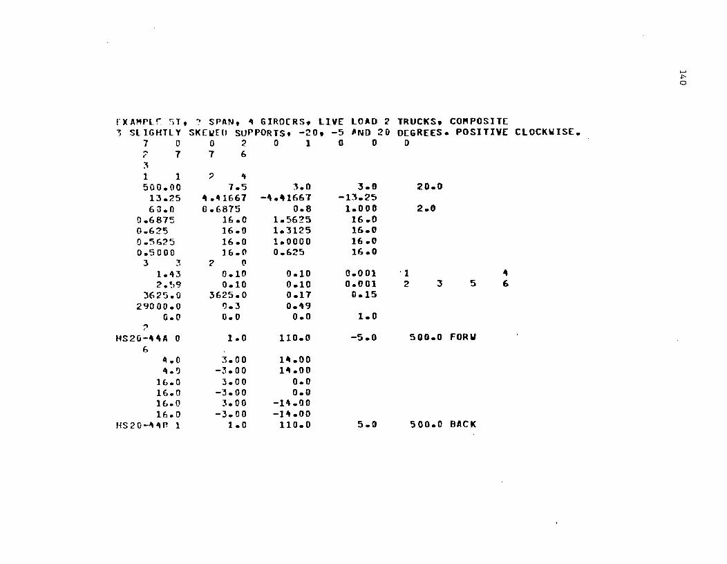
rXAMPLf ~l, ~ SPAN, ~ GIRDERS. LIVE LOAD 2 TRUCKS. CO"POSITE ~ SLIGHTLY SK[,,[[) SUPPORTS, -20. -5 liND 20 D[GREES. POSITIVE ClOCK ... IS[.
7 0 0 2 0 1 0 0 0
'" 1 7 6 .t'.
3 1 1 ? '4 500.00 1.5 3.0 3.0 20.0
13.25 0\.41661 -".~1667 -13.25 6 0.0 0.6875 0.8 1.000 2.0
0.6875 16.0 1.5625 16.0 0.625 16.0 1.3125 16.0 0.5';25 16.0 1.0000 16.0 0.5000 16.0 0.625 16.0
3 3 2 ('
1.43 0.10 0.10 0.001 '1 4 2.~,9 0.10 0.10 0.001 2 J 5 (,
3625.0 3625.0 0.17 0.15 29000.0 rJ.3 0.1\9
0.0 0.0 0.0 1.0 ::'
HS20-lfitA 0 1.0 110.0 -5.0 500.0 FORV 6
~.O 3.00 14.00 q.1) -3.00 14.00
H .. O 3.00 0.0 16.0 -3.00 0.0 1£ •• 0 3.00 -14 .00 16.0 -3.00 -11f.00
HS20-ItIfP. 1 1.0 110.0 5.0 500.0 BACK
...... .,... o
1 0.0
10.0 20.0
t'!
2 2 It 1
r ... ~
~ 1
11 10
1.375 1.187~;
1.0000 0.6875
0 ~ ') , 1 ~ ":J
1).0 10.0 20.0
0 ? 2
-20.0 -10.0
0.0
HaO 4
1 1.0
0 Hi .0 16.0 16.0 U;.o
I :20.0
0.0 -5.0
0 .. 0
1.6875 1.11375 1.25 0.87'5
16.0 11;.0 16.0 16.0
~
~ ~

1 .4\
iJ :? Ji 1 :5
11 10 0.6815 0.625 O.562~
O.5:JOO J
'3 ? 1
" 3 0.0 1.~
15.0 CI
1 16.0
0\ 1000.0 3£.25.0
0 16.0 H .. O HuO 16.0
1 20.0
0.0 7.5
15.0
1.5625 1.:.'H 25 1.0000 0.625
16.0 16.0 16.D 16.0
t-' J::tv
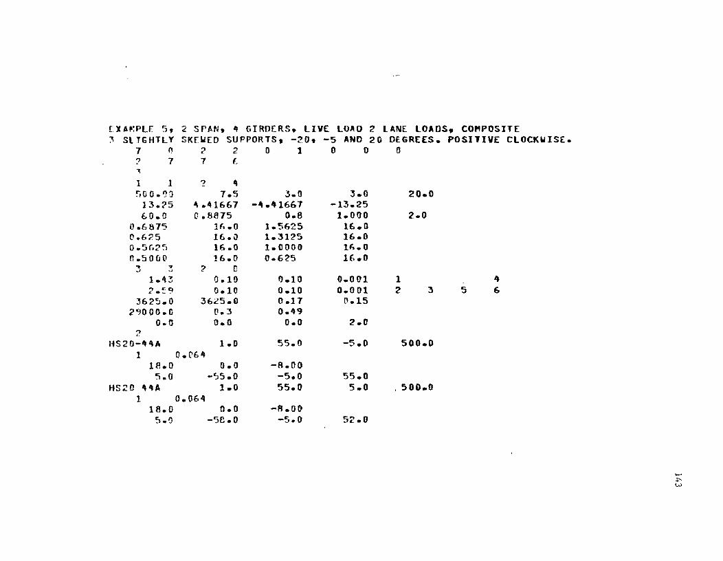
(XAP'.PL[ 5, :-, SlTGHTLY
7 () :> 7 ~
1 1 ~,(j o. IJO 13.~5
60.0 0.6875 O.6:?5 0.5(.25 0.5000 ~
, -! .J
1 .. ~3 7.~9
3625.0 29000.11
o.n ") t.
IiS20-44A 1
18.0 5.0
HS21l ,. .. A
1 18.0 5.~
2 SPAN, ~ GIRDERS. LIVE LOAD 2 LANE LOADS. CO"PQSITE SK[~ED SUPPORTS, -20, -5 AND 20 DEGREES. POSITIVE CLOCKWISE.
.7 2 0 1 000 7 (
~ " 7.5 3.D " .'''1667 -4.41667 0.8875 0.8
16.0 1.5625 16.0 1.:5125 16.0 1.0000 16.0 0.625
? t:l 0.1!) 1).10 0.10 0.10
3625.0 0.17 0.3 0.49 0.0 0.0
1.0 55.0 O.()6'l
0.0 -R.OO -":>5.0 -5.0
1.0 55.0 0.(164
n.o -R.OO -'5f!.O -5.0
J.O -13.25
1.000 16.0 16.0 HieD 1£ •• 0
0.001 0.001
0.15
2.0
-S.O
55.0 5.0
52.0
1 2
20.0
2.0
J
500.0
, 500.0
5
,. (,
!-' ..,.. LV

144
cc CI
• • • o C'> C N -I I
0"- M C Q
• • ..:;, M .... 00 0
• • • 0 Q I:) -N
- C (" ~ .... (\ "" .... .... c: .... .... r;;; 0
eoce • • • • >.tJ~~..c ............ ..-1
l.I"'IlI" ,...,... !/'I COl"') \f'l"" \D~ (1,1;:0
• • • • .... ...c .... 0
(:) Cl oc • • • • >.tJ\D ..r,\D
"'"' .... HM
If' 10; QU": ,...,... c,... fO"')ct) oct) l...c CloD
M • • • .... .... 9
cc c • • •
o "J 0 I
.... 0 .... • 0
N
(.;I I;) (:)
• • • 000
.... C\: ";('.IMq ." :~ (' • .-I
c.. .:=
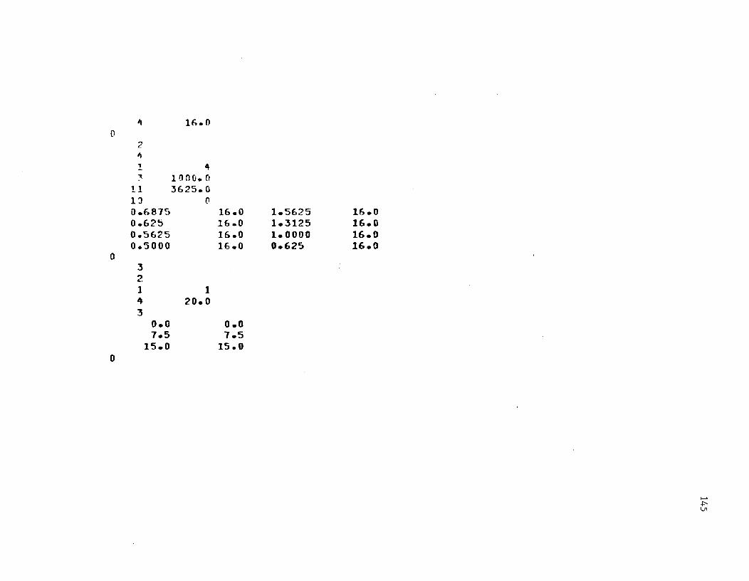
14 0
2 'I !. ~
11 1:1 o .687~) 0.625 0.5625 O.SOOO
0 3 2 1 4 3
0.0 7.5
15.0 0
16.0
14 1000.0 3625.0
(l
16.0 1£ .. 0 16.0 16.0
1 20.0
0.0 7.5
15.0
1.5625 1.3125 1.0000 0.625
16.0 16.0 16.0 16.0
I-' .p\J1

[XA~PL( 60, 2 SPAN. 0\ GIRDERS, DEAD 3 SLIGHTLY SKr~EO SUPPORTS, -~O, -5
7 I) 0 1 0 1 0 ~ 7 7 6 :'5 1 1 2 0\
-soo.no 7.5 3.0
LOAD I, NON-CO~POSITE AND 20 DEGREES. POSITIVE CLOCKWISE.
o 1
3.0 20.0 13.25 ,. .41667 -1f.41667 -13.25 6/).0
O.687"i !J.625 0.5625 0.5COO
'3 3 1.Al3 2.~q
1.0 29000.0
0.0 1
0.0 11).0 20.0
f)
'? " . ... , 14
1 J
0.6875
2
16.0 4
16.0 16.0 16.0 16.0
0 0.10 0.10 1.0
0.3 0.0
-?o.o -IC.O
['.0
0.8 1.5625 1.3125 1.0000 0.625
0.10 0.10 0.11 0.49 0.11
1.000 16..0 16.1} 16.0 16.0
0.001 0.001 0.15
0.0
2.0
1 '2 J 5
If 6
I-' ./>
'"
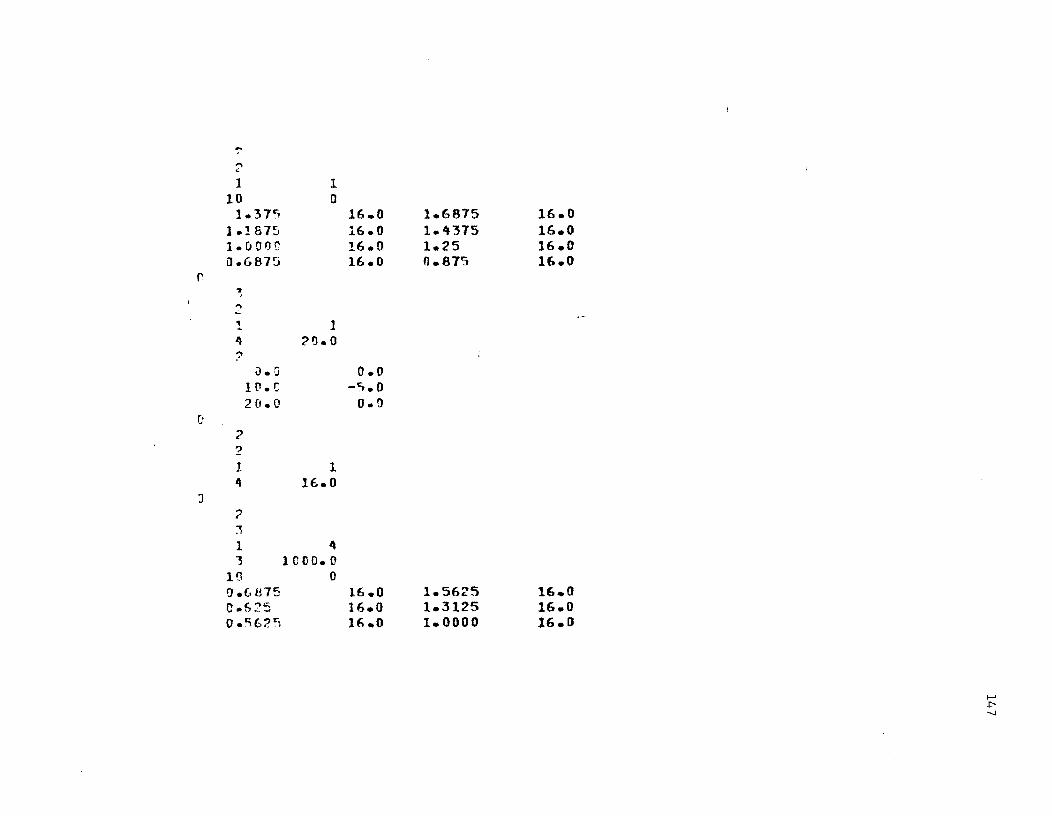
~
... " 1
10 1.37c;
1.! 875 1.IJOOr iJ.6875
r ~ , ... ,;..
1 4 ?
i).D Ill.r:: 20.0
0 ? :2 1 4
J ? :1 1 1
HI 0.(, 815 0.625 o .E:i62!"1
1 0
16.0 16.0 16.0 16.0
1 2~.O
0.0 -5.0
0.1]
1 16.0
~
1000.0 0
16.0 16.0 16.0
1.6875 1.1+'375 1.25 0.875
1.5625 1.3125 1.0000
16.0 16.0 16.0 16.0
16.0 16.0 16.0
!-' .P-.J
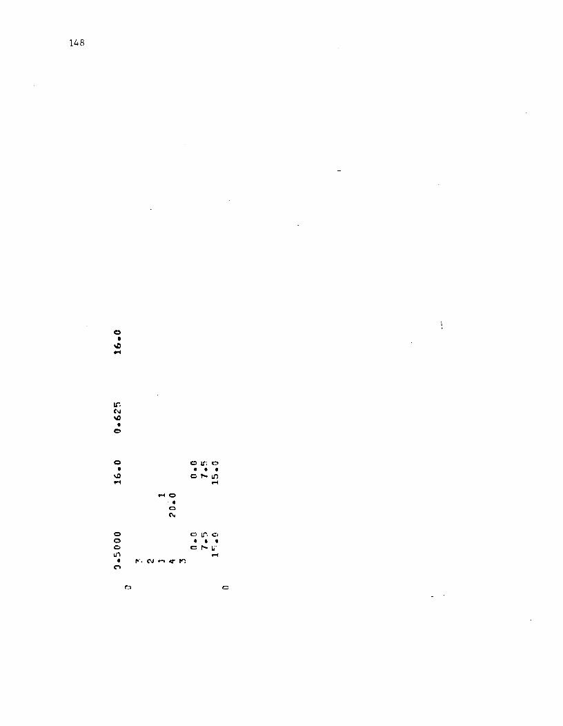
148
o • \0
pol
o •
\D pol
t-10 ., o ('I,j
01(; 0
• • • Cpo..&n
Pi
o 01/"',0 o • • • o c po..~. Ln _
, ,.., (\J ..... IZ' n ~
o
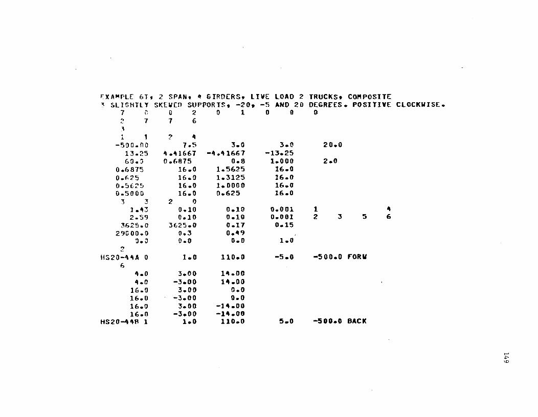
~XAMPLE 6T, 2 SPAN, ~ GIRDERS, LIVE LOAD 2 TRUCKS, CO"POSITE ~ SLIGHTLY SK[~En SUPPORTS, -20, -5 AND 20 DEGREES. POSITIVE CLOCKWISE.
1 0 0 2 0 1 0 0 0 ... 1 1 6 ... , . 1 2 4 ....
-500.no 1.5 3.0 3.0 20.0 13.25 ,..-\1667 -4.1f 1667 -13.25 60.3 0.(.815 0.8 1.000 2.0
0.6875 16.0 1.5625 16.0 0.625 16.0 1.3125 16.0 0.56:-'5 16.0 1.0000 16.0 0.5000 16.0 0.625 16.0
J :3 2 I)
1.~3 0.10 0.10 0.001 1 4 2.59 0.10 0.10 0.001 '2 3 5 6
;'6.25.0 3625.0 0.11 0.15 29000.0 0.3 O.~9
n.D 0.0 0.0 1.0 ?
HS20-'''A 0 1.0 110.0 -5.0 -500.0 '-ORY f,
1f.0 3.00 14.00 If.O -3.00 14.00
16.0 3.00 0.0 16.0 -3.00 0.0 16.0 3.00 -14.00 16.0 -3.00 -14.00
HS20-44-R 1 1.0 110.0 5.0 -500.0 BACK
.....
.p\0

150
f"1
000 , , . ooc:. t\;0-4 I I
(;">00
• • • 000
0-4 C,J
('. C\J C' ..... C,_ I'": ..... 0-4 0 .... .-1
OOOc • •••
\00)\,1:1\,1:1\0 .... 0-41""1 ...
iI1Jr. ,... .... I/" a) ~ I:") .... ..c.,..(\JCC
• • • • ... 0-4 .... C'l
c>coo • • • • ;J;~..s;J..c ..................
LI- t!' a 1/", .... ,... 0 l-PO) .:0 0 CO
• ..... 1..:1 \C. .... • • • ..... 0-4Q ,. .. , C'.! rl 4"(\.
ceo • •• Qltlo
I
CJC 0 t • • 0.;;) 0
0-4 (\, C'J (\j

1 4
I)
2 It-t 3
11 If)
0.6815 0.625 O.5(;2~i
0.5000 (\
:3 ~
1 ~
:3 :>.0 7.5
1'5.0 0
1 H ... O
~
100J.O 3625.0
0 16.0 16.0 16.0 16.0
1 20.0
0.0 7.5
15.0
1.5625 1.3125 1.001l0 0.625
16.0 16.0 16.0 16.0
...... VI ......

rXAMPLE bLl 2 SPAN, ~ GIROERS, LIVE 3 SLIGHTLY SKEWED SUPPORTS, -20, -5
7 0 £' '2 0 1 0 2 7 7 (, 3 1 1 ? 0\
-500.flO 7.5 3.0
LOAD 2 LANE LOADS, COMPOSITE AND 20 DEGREES. POSITIVE CLOCKWISE.
o 0
3.0 20.0 13.2'5 " .0\1661 -oIl.'l1667 -13.25 60.0 0.8815
ll.f. 1115 16.0 0.625 16.0 il.S&2~ 16.0 O.5DOO H .. O ~ 3 '2 0
1.~3 0.10 '2.59 0.10
3'>2'5.0 3625.0 29000.0 0.3
0.0 0.0 ?
HS;;O-~ 4 A 1.0 1 0.064
IIl.O 0.0 ':") . () -:15.0
HS20 4~A 1.0 1 0.064
18.0 0.0 "l.o -58.0
0.8 1.5625 1.3125 1.0000 0.625
0.10 0.10 0.17 0.49 0.0
55.0
-8.IJO -5.0 55.0
-8.00 -5.0
1.000 16.0 16.0 16.0 16.0
0.001 0.001 0.15
2.0
-5.0
55.0 5.0
52.0
1 2
2.0
:3
-500.0
-500.0
5 " 6
I-' VI N
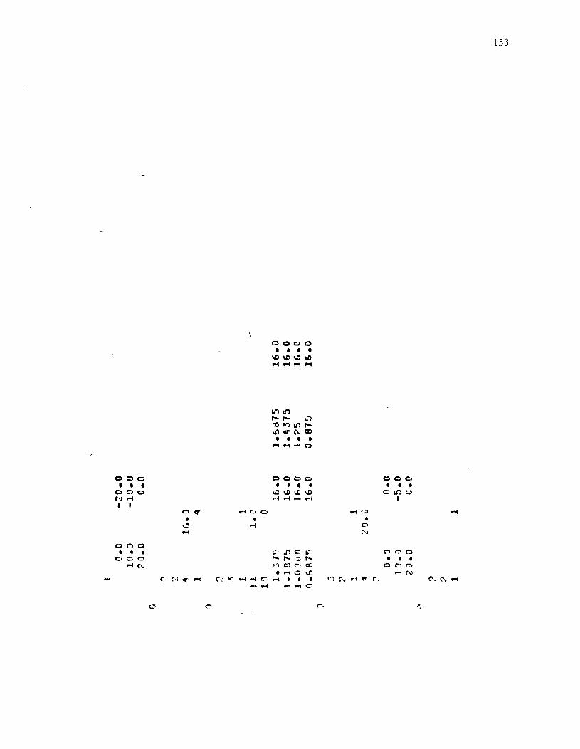
0 c c • • • 0 0 c
C'J ~ I I
C'l cr ~i 0 C I I
\0 M .... 0 CJ 0
I • I 0 c:. 0
P"I (,,,
M C' {'I cr' .... C' ~ I"': r-i M C.
-- .-I
ooco • • • • \DIoO\O\D ~~~P"I
Ifltn .......... L.~ ~l'1tn,... ..oC'(\JCD
• I • • ........ ~o
c 00 C> I I • I
\C ..o..o~ M M ~ 0-1
~, ... 0 Ii I"- ..... 0 ..... ~') 0 r.. ex:.
I M U \C .... • • • P"I .... 0
("".
153
Q O~ I • I
0 1.(;0 I
.... 0 I
0
'" C"> C:> Q
I I I 0 0 0
M N n C' .. rl ~ r". (\.; r-. ....

154
<Ir co • • c,L."";
ON 0"" ~ ""J
c:;.
CCOO
• ••• '00'00\00100 ..................
\n\n0 NNo",", ..cf"4C'>C\J it'\f")O\ll
• • • • .... .... H CJ
0000
• ••• \.O<.C\.O..c .... H .... o-1
~-, .... -. (';)
,.... ~'") r'. 0 r:t)('\J..oo
\0 ~ Ltlll'l C'\i<C/" .... t<; .... o ••••
... f"40 c.' 0 <:)
OIl'lO • • •
o""'Ln ....
01f'0
• • • o ,....~,
....

APPENDIX C
GRAPHICAL DISPLAY OF INPUT DOCUMENTATION
155

GUIDE FOR INPUT DATA
SECTION 2.4.1 INITIAL DATA FOR PROGRAM
A) Control Cards
1
1
2
1
3
Identification of run (two lines)
Control card
I Nogp I Ipl Ildef I Jrec I Irec I IrcsuJlj NosPij Kgen I K--ompj
1 6 11 16 21 26 31 36 41 45
B) Support conditions
Nsubbc,l), Nsubbc(2)
I Nspanl Nfix I t I J( I (3) I (4) I (5) I (6) I (7) I (8) I (9) I (10) J 1 (I) 6 (I) 11 (I) 16 (I) 21 (I) 26 (I) 31 (I) 36 (I) 41 (I) 46 (I) 51 (I) 56 (I) 60
80
80
t-' \.Jl
'"

C) Prescribed suppon conditions
I Jspg I Kspg I Vspg 1 (I) 6 (I) 11 (I') 20
Nospgtimes
D) Erection Procedure
Kgrst Kgren Ksbst
1 (I') 11 (F) 21 (I')
Irec times
SECTION 2.4.2 IROUTE = 1
A) Substructure index
I Iroute 1=1 1 (I) 5 B) Bridge Geometry 1 I Nv I Idivt I Idivll Ngk I 1 (I) 6 (I) 11 (I) 16 (I) 20
Ksben
31 (I') 40
,...... \.Jl '-.I

2
Rref Tc Ovin Ovout Sdia
1 (F) 11 (F) 21 (F) 31 (F) 41 (F) 50
C) Girder information
I Rgir(1) Rgir(2) I Rgir(3) Rgir(4) I Rgir(5) Rgir(6) I Rgir(7) Rgir(8)
1 (F) 11 (F) 21 (F) 31 (F) 41 (F) 51 (F) 61 (F) 71 (F) 80
I .. Ngir times
2
I Girdwd I Tw I Tftavg I Ttbavg Soff
1 (F) 11 (F) 21 (F) 31 (F) 41 (F) 50
3
Tft Bft I Ttb Btb J 1 (F) 11 (F) 21 (F) 31 (F) 40
Ngir times
t-' V1 (Xl
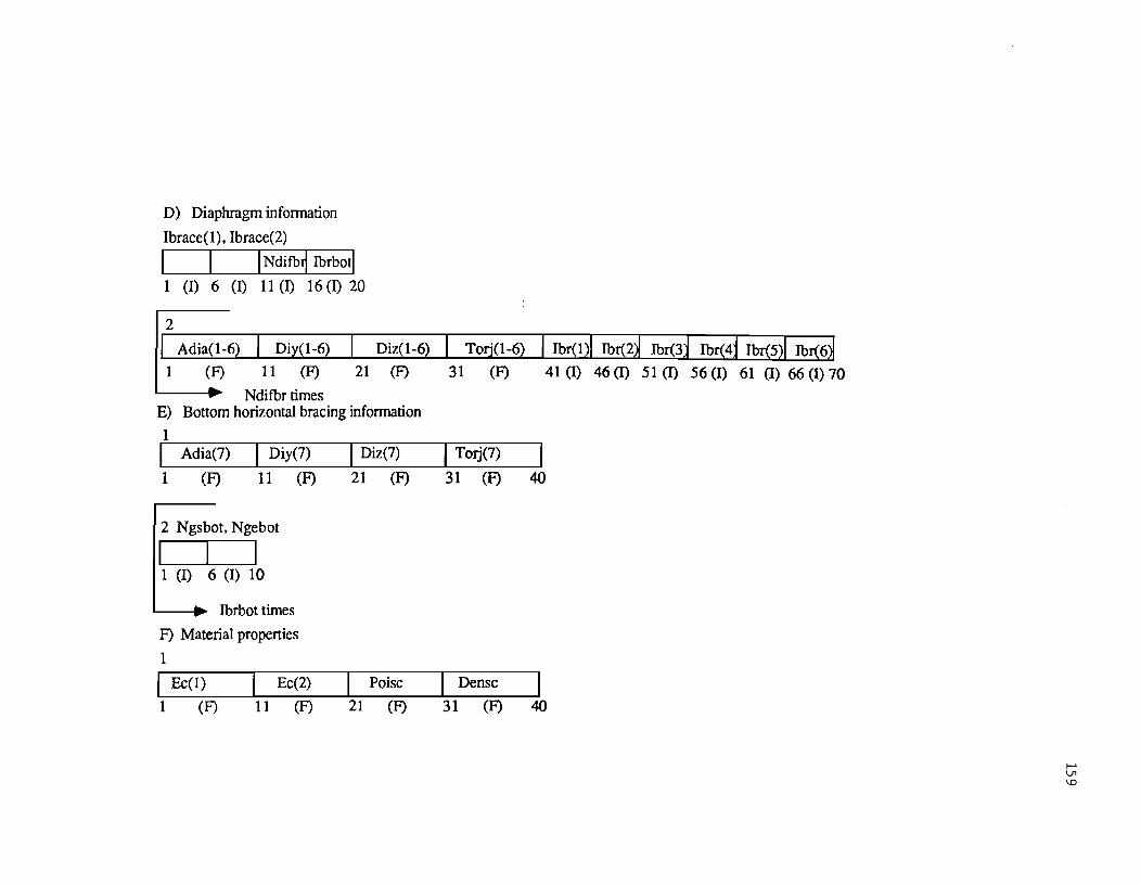
D) Diaphragm information
Ibraee(I), Ibraee(2)
I Ndifb~ Ibrbotl
1 (I) 6 (I) 11 (I) 16 (I) 20
2
Adia(I-6) Diy(1-6) Diz(I-6) Torj(1-6) I Ibr(1)1 Ibr(2~ Ibr(3~ Ibr(4j Ibr(5) I Ibr(6~ 1 (F) 11 (F) 21 (F) 31 (F) 41 (I) 46 (I) 51 (I) 56 (I) 61 (I) 66 (I) 70 L--_.~ Ndifbr times E) Bottom horizontal bracing information
1 Adia(7) I Diy(7) I Diz(7) I Torj(7)
1 (F) 11 (F) 21 (F) 31 (F) 40
2 Ngsbot, Ngebot
I I I 1 (1) 6 (1) 10
L....---t.~ Ibrbot times
F) Material properties
1
I Ec(1) Ee(2) I Poise I Dense
1 (F) 11 (F) 21 (F) 31 (F) 40
t-' V1 \0

2
Est Poisst Densst
1 (F) 11 (F) 21 (F) 30
G) Slab load infonnation
Curbld(l) Curbld(2) Surfld
1 (F) 11 (F) 21 (F)
H) Truck load infonnation (Zlivld = 1.0)
1
I Ntrucq
1 (I) 5
2 Ibid
Zlivld
31 (F) 40
I Name [ I Dlf Xpos I Ypos Radtr I Idir I 1 (A) 9(1) 11 (F) 21 (F) 31 (F) 40 50 52 (A) 55
3
UNwheel 1 (1) 5
4
Trld Centtr Cendg J 1 (F) 11 (F) 21 (F) 30
Nwheel times
L-------I ........ Ntruck times
,...... Cl' o

I) Lane load infonnation (Zlivld = 2.0)
1
I Nlanl~ 1 (I) 5
2
I Name II Dlf Xpos Ypos Radln
1 (A) 8 11 (F) 21 (F) 31 (F) 40 50
3
INconl~ Wdist 1 1 (I) 6 (F) 1
r Trl: I Cent" Centlg 1 (F) 11 (F) 21 (F) 30
Nconld times
Wy(l) Wx(l) Wy(2) Wx(2)
1 (F) 11 (F) 21 (F) 31 (F) 40
'---------j .. ~ Nlanld times J) Additionalloads
I Idof IJsubldl Kelno rill P(I) P(2) P(3) P(4) J 1 (I) 6 (I) 11 (I) 15 21 (F) 31 (F) 41 (F) 51 (F) 60
...... 0' ......

SECTION 2.4.3 IROUTE = 2
A) Substructure index
1
I Iroute I = 2
1 (1) 5
B) Number of values to be changed
I Novall
1 (1) 5
C) Update of values
II NaIl; Value I 1 (1) 6 (F) 15
Noval times
D) Additionalloads
11 (I) 15
P(I)
21 (F)
P(2) P(3)
31 (F) 41 (F)
P(4)
51 (F)
60
...... ~ N

SECTION 2.4.4 IROUTE = 3
A) Substructure index
1 -3
I Iroute I -1 (I) 5
B) Data for Either sections 2.4.2 or 2.4.3
C) Slight skew support placement
INsbc I 1 (I) 5
D) Slight skew mesh geometry
~l Dsks I Dske
1 (F) 11 (F) 20
(Idivl + 1) times
E) Additionalloads
lldof IJSubldlKeln0WIII P(l) P(2) P(3) P(4)
1 (I) 6 (I) 11 (I) 15 21 (F) 31 (F) 41 (F) 51 (F) 60
....... aw

SECTION 2.4.5 IROUTE = 4
A) Substructure index
1
I Iroute I = 4
1 (I) 5
B) Data for Either sections 2.4.2 or 2.4.3
C) Severe skew support placement
I Ngs I Nge I 1 (I) 6 (I) 10
E) Additionalloads
P(1)
21 (F)
P(2) P(3)
31 (F) 41 (F)
P(4)
51 (F) 60
I-' (J\
~

SECTION 2.4.6 IROUTE = 5
A) Substructure index
I Iroute I = 5 1 (1) 5
B) Control cards for this substructure
I Noeq Noptl Nv I RO 1 (1) 6 (I) 11 (1) 16 (F) 25
C) Element node numbers for this substructure
I i I J K L 1 (I) 6 (I) 11 (I) 16 (I) 20
'-----P'" Noel times
D) Cylindrical coordinates (RO> 0, RO < 0)
D A z 1 (I) 5 11 (F) 21 (F) 31 (F) 40
t-'
'" V1

E) Cartesian coordinates
III 7I~ : -11 (~ 21 ;: 31 ~ I:i~ 1~1~I:i;~ 1:6;~ I~~ I::~ 170 Nopttimes
F) Element types and material properties Use the same order of elements as in section 2.4.6, part C.
Web elements =0
I Nodes I Ntri I QuadtlKbcaml E1 E2 Thq V21 Gm
1 (I) 6 (I) 11 (I) 16 (I) 21 (F) 31 (F) 41 (F) 51 (F) 61 (F) 70
Slab elements = 1
I Nodesl Ntri I QuadtlKbeaml E1 E2 Thq V21 Gm
1 (I) 6 (I) 11 (I) 16 (I) 21 (F) 31 (F) 41 (F) 51 (F) 61 (F) 70
Beam elements =2 =0
Range elements
=2 = 1
Em A Gm Tf Bf
1 (I) 5 16 (I) 21 (F) 31 (F) 41 (F) 51 (F) 61 (F) 70 (F) 80
...... (J\ (J\

Rigid link elements =2
G) Number of elements per each substructure
1 (I) 6 (I) 11 (I) 16 (I) 21 (I) 26 (I) 31 (I) 36 (I) 41 (I) 46 (I) 51(1) 56 (I) 61 (I) 66 (I) 71 (I) 76 (1) 80
I ... Nv times
H) Control cards for this substructure
= 1
I) Substructure master nodes Oocal nodes which will be renumbered to master nodes)
J) Nodes having boundary conditions excluding master nodes
I Node I Bc-x I Bc-y IBC-Z I Bc-xxIBC-yy I BC-zz I 1 (I) 6 (I) 11 (I) 16 (I) 21 (I) 26 (I) 31 (I) 35
Mas(2) times
~ 0\
"""

K) Specified boundary conditions for non-master nodes
II X-tran: I Y-tI1Ins I Z-trans I X-rot Y-rot Z-rot 1 (F) 11 (F) 21 (F) 31 (f') 41 (f') 51 (f') 60
Lpgi5 times
L) Input required for data generator program
I Nxnd I Nbc51Lpgo51 Deent5
1 (I) 6 (I) 11 (I) 16 (F) 25
M) Boundary condition codes for master nodes of this substructure
I Node I Bc-x I Bc-y I Bc-z I Bc-xx I Bc-yy IBc-zz I 1 (I) 6 (I) 11 (I) 16 (I) 21 (I) 26 (I) 31 (I) 35
'-----~~ Nbc5 times
N) Specified boundary conditions for master nodes
II X-trans. I Y-trans I Z-trans I X-rot Y-rot Z-rot 1 (f) 11 (F) 21 (F) 31 (F) 41 (f) 51 (f) 60
Lpgo5 times
0) Additionalloads
I Idof IJsubldl Kelno'. P(1) P(2) P(3) P(4)
1 (I) 6 (I) 11 (I) 15 21 (f) 31 (F) 41 (f) 51 (F) 60
t-' (j\
00

BIBLIOGRAPHY
1. "Guide Specifications for Horizontally Curved Highway Bridges," The American Association of State
Highway and Transportation Officials, Washington D.C., 1980.
2. Heins, C. P., Bending and Torsional Design in Structural Members, D. C. Heath and Company, 1975.
3. Heins, C. P., "Steel Curved I and Box Girder Design and Analysis," Analysis and Design of Bridges,
Martinus Nijhoff Publishers, The Hague, 1984.
4. "V -Load Analysis: An Approximate Procedure, Simplified and Extended, for Determining Moments and
Shears in Designing Horizontally-Curved Open-Framed Highway Bridges," USS Highway Structures
Design Handbook, Chapter 12, Vol. 1.
5. Timoshenko, S. P., Theory of Plates and Shells .. McGraw-Hill, New York, 1959.
6. Brockenbrough, R. L., "Distribution Factors for Curved I-Girder Bridges," Journal of Structural
Engineering .. Vo1.112, No. 10, October 1986.
7. Heins, C. P., "Box Girder Design," AISC Engineering Journal, Vol. 15, No.4, Dec 1978.
8. Wilson, L., Bathe, KJ., Peterson, F.E., Dovey, H., "User's Guide to Program SAP," University of Calif.
Dept of Civil Engineering, Nov. 1972.
9. Schelling, D.R., Heins, C.P., Sikes,G.H., "State of the Art of Curved Girder Bridge Programs,"
Computer and Structures, Vol. 9, pp. 27-37, Pergamon Press, London, 1978.
10. Heins, C.P., Sahin, A., "Natural Frequency of Curved Box Girder Bridges," ASCE St. Div. Journal., Vol.
105, No. ST5, May 1979.
11. Heins, C.P., Sheu, F.H., "Computer Analysis of Steel Box Girder Bridges," Civil Engineering Dept.
Report Univ of Maryland, June 1981.
12. Heins, C. P., Olenick).C., "Curved Box Beam Bridges Analysis, " Computer and Structures Journal,
Vol. 6, pp. 65-73, Pergamon Press, London. 1976.
169

170
13. Weaver, W., Johnson,P.R., Finite Elements for Structural Analysis, Prentice-Hall, Englewood Cliffs, New
Jersey, 1984.
14. Fiechtl, A., Fenves, G. L., Frank, K. H., "Approximate Analysis of Horizontally Curved Girder Bridges,"
Research Report No. 360-2F, Center for Transportation Research, The University of Texas at Austin,
November 1987.
15. Davis, B.G., Hoffman, T.R., Fortran: A Struclured, Disciplined Sryle,.McGraw-Hill, New York, 1983.
16. Yargicoglu, A., Johnson, C.P., "Temperature Induced Stresses in Highway Bridges by Finite Element
Analysis and Field Tests," Research Report No. 23-3F, Center for Highway Research, The University of
Texas at Austin, July 1978.
17. Johnson, C.P., Thepchatri, T., Will, K., "Static and Buckling Analysis of Highway Bridges by Finite
Element Procedures," Research Report No. ISS-IF, Center for Highway Research, The University of
Texas at Austin, 1973.