Analysis Methods for Water Distribution Systems-3rd Class

1

تسم الله الزحمه الزحيم

Analysis Methods for Water Distribution Systems-3rd

Class

)طرق تحليل أنظمة توزيع المياه(Dr. Sataa A. Al-Bayati (10-11)

Methods of analysis are:

1. Sectioning)المقاطغ(

2. pipe equivalence)الاوثىب المكافىء(

3. Relaxation)الارخاء(

4. Computer programming)الثزمجح تالحاسىب(

5. Electrical analogy )المشاتهح الكهزتائيح(

6. Linear theory )الىظزيح الخطيح(

7. Heasted)هيسرذ(

8. Newton Raphson)ويىذه رافسىن(

The purpose of these methods is to find the discharge for each pipe & the

pressure at each junction (node ػقذج(.

1.Method of Sections It is quick, approximate, exploratory أسرطلاع() , & simple.

Steps:

1. Cut the network by a series of line

Not necessarily straight or regularly spaced.

It chosen with regard to varying sequence of pipe sizes &

district characteristics.

The lines may cut the pipes at right angles to the general

direction of flow.

Lines may be horizontally.

For more than one supply conduit, lines may be curved.

2. Estimate the demand for each areas beyond each section, depends on;

a) Population density.

b) Characteristics of zone: residential, industrial, commercial,

etc.

2

The demands are:

a) Domestic: decreases from section to section.

b) Fire, Table (1)

It remains the same until high value district has been passed.

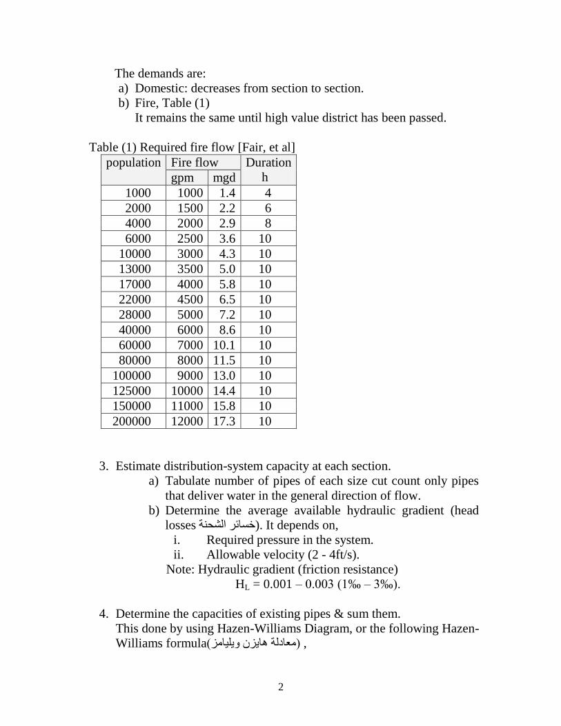
Table (1) Required fire flow [Fair, et al]

population Fire flow Duration

h gpm mgd

1000 1000 1.4 4

2000 1500 2.2 6

4000 2000 2.9 8

6000 2500 3.6 10

10000 3000 4.3 10

13000 3500 5.0 10

17000 4000 5.8 10

22000 4500 6.5 10

28000 5000 7.2 10

40000 6000 8.6 10

60000 7000 10.1 10

80000 8000 11.5 10

100000 9000 13.0 10

125000 10000 14.4 10

150000 11000 15.8 10

200000 12000 17.3 10

3. Estimate distribution-system capacity at each section.

a) Tabulate number of pipes of each size cut count only pipes

that deliver water in the general direction of flow.

b) Determine the average available hydraulic gradient (head

losses خسائز الشحىح). It depends on,

i. Required pressure in the system.

ii. Allowable velocity (2 - 4ft/s).

Note: Hydraulic gradient (friction resistance)

HL = 0.001 – 0.003 (1‰ – 3‰).

4. Determine the capacities of existing pipes & sum them.

This done by using Hazen-Williams Diagram, or the following Hazen-

Williams formula مؼادلح هايزن ويليامز() ,

3

Q = 0.27853 C D2.63

S0.54

Where:

Q = capacity, mgd

C = roughness constant خشىوح(الثاتد ) ,

D = pipe diameter, ft

S = slope, or hydraulic gradient.

We can use a diagram for quick calculation.

5. Calculate deficiency)ػجز(

Deficiency = required capacity – existing capacity.

6. Modified system

For the available hydraulic gradient, select the sizes & routs of pipes

to cover deficiency. Some existing small pipes may be removed to

make way for larger mains.

Adding or removing pipes done according to the designer. If the

deficiency is small no pipes are added but the velocity & head loss

must be within the limits. If the deficiency is large the pipes must be

added or changed with larger sizes.

7. Determine size of equivalent pipe for the modified system & calculate

velocity.

Reduce high velocity by lowering the HL.

8. Check important pressure requirements against modified network.

Usefulness of section method:

1. For preliminary أوليح() studies of large & complicated distribution

systems.

2. Check upon other methods of analysis.

Example (1):

Analyze the network of the following Fig. by section method. The hydraulic

gradient available within the network is 2‰. The value of C = 100 in the

Hazen-Williams formula, and the max. daily use (domestic demand) =

150gpcd. The fire demand is taken from Table (1). Population as follows,

Section a-a b-b c-c d-d e-e

Population 16000 16000 14000 8000 1500

4

Note: All pipes without number are 6-in diameter.

Solution:

1. Section a-a

Population = 16,000

a) Total demand = domestic use + fire demand

= 16,000 × 150gpcd + 5.6mgd

= 2.4 + 5.6

= 8mgd.

b) Existing pipes)الاواتية المىجىدج(:

One 24in

HL = 0.002 → Hazen-Williams Diagram → Q = 6mgd.

5

c) Deficiency:

8 – 6 = 2mgd (large deficiency)

d) If no pipes are added,

The 24in must carry Q = 8mgd.

Diagram → HL = 0.0033 ≈ 3‰ OK, why excepted?

V = 3.85fps < 4fps OK

2. Section b-b

Population = 16,000

a) Total demand = 8mgd

b) Existing pipes:

2 – 20in → 20in & HL = 0.002 → Diagram → Q20in = 3.7mgd

Q2- 20in = 3.7 × 2 = 7.4mgd.

c) Deficiency:

8 – 7.4 = 0.6mgd (low deficiency)

d) No pipes are added,

The 2 – 20in must carry Q = 8mgd.

Q = 7.4mgd & HL = 0.002 →Diagram → Equivalent pipe= 26in

Q = 8mgd & Dia.= 26in → Diagram → HL = 0.0022 < 3‰ OK

V = 3.2fps < 4 OK

3. Section c-c

Population = 14,000

a) Total demand = 14,000 × 150 + 5.6

= 2.1 + 5.6

= 7.7mgd.

b) Existing pipes:


2 – 12in → 12in & HL = 0.002 → Diagram → Q12in = 1mgd

Q2-12in = 2mgd


Q5-6in = 0.8mgd

Total Q = 3.7 + 2 + 0.8 = 6.5mgd.

6

c) Deficiency:

7.7 – 6.5 = 1.2mgd (large deficiency).

d) Pipes added & removed:

Pipe added:


Q2-10in = 1.2mgd

Pipes removed:


Net added capacity = 1.2 – 0.2 = 1.0mgd.

e) Modified capacity = 6.5 + 1.0 = 7.5mgd

Q = 7.5mgd & HL = 0.002 →Diagram → Equivalent pipe= 26in

Modified system must carry Q = 7.7mgd,

Q= 7.7mgd & Dia.= 26in →Diagram→ HL = 0.0021 < 3‰ OK

V = 3.1fps < 4 OK

The layout after analyzing section c-c is:

7

4. section d-d

Population = 8,000

a) Total demands = 8,000 × 150 + 5.6

= 1.2 + 5.6

= 6.8mgd.

b) Existing pipes:

2 – 12in → 12in & HL = 0.002 → Diagram → Q12in = 1mgd

Q2-12in = 2mgd


Q8-6in = 1.3mgd

Total Q = 2 + 1.3 = 3.3mgd.

c) Deficiency:

6.8 – 3.3 = 3.5mgd (large deficiency).

d) Pipes added & removed:

Pipes added:



Q2-10in = 1.2mgd

Total pipes added, Q = 3.3mgd.

Pipes removed:


Q2-6in = 0.3mgd

Net added capacity = 3.3 – 0.3 = 3mgd.

e) Modified capacity = 3.3 + 3 = 6.3mgd

Q=6.3mgd & HL =0.002 →Diagram → Equivalent pipe= 24.4in

Modified system must carry Q = 6.8mgd,

Q= 6.8mgd & Dia.=24.4in →Diagram→HL =0.0022 < 3‰ OK

V = 3.2fps < 4 OK

The layout after analyzing section d-d is:

8

5. Section e-e

Population = 1,500

a) Total demands = 1,500 × 150 + 1.8

= 0.2 + 1.8

= 2mgd.

b) Existing pipes:


Q2-8in = 0.7mgd


Q6-6in = 1mgd

Total Q = 0.7 + 1 = 1.7mgd.

c) Deficiency:

2 – 1.7 = 0.3mgd (low deficiency).

d) Pipes added & removed (previously):

Pipes added:

9


Pipes removed:


Net added capacity = 0.6 – 0.16 = 0.4mgd.

e) Modified capacity = 1.7 + 0.4 = 2.1mgd

Q=2.1mgd & HL =0.002 →Diagram → Equivalent pipe= 15.8in

Modified system must carry Q = 2mgd,

Q = 2mgd & Dia.=15.8in → Diagram → HL = 0.002 < 3‰ OK

V = 2.3fps < 4 OK

The modified system is shown in the following Fig.

Final layout of the network

10

Circle Method)طريقة الدائرة(

It is sectioning method. It is used for design or investigates ذحقق() the

minor pipes.

Example (2):

Assuming water is to be delivered to a fire through not more than 500ft

of hose. Find by circle method, the water available at the circumference

of a 500 ft circle placed in the center of the shown network. Also find the

number of hydrants, if the capacity of each one is 250gpm. The pressure

in the 12in feeders مغذياخ() being 40 psi & the residual hydrant pressure

not less than 20 psi. Take C = 100 in the Hazen-Williams formula.

-N-

Feeder: 12-in

Lateral: 6-in

11

Solution:

The pipes cut by the circle, the average length of these pipes from their

feeder مغذي() pipes to the hydrants within the circle, & the hydraulic

gradients of these pipes:

1. Hydraulic Gradients:

North-South;

4-6in, length = 1000 – ½(500) = 750ft.

H. gradient, S = h/L = (P/γ)/L = P/γL

S = [(40 – 20)Lb/in2 × (144in

2 /ft

2)] / (62.4Lb/ft

3)(750ft)

= 0.0616

= 61.6‰

East-West;

4-6in, length = 1250 – ½(500) = 1000ft.

H. gradient, S = (20 × 144) / (62.4 × 1000)

= 0.0462

= 46.2‰

2. Pipe capacity

C = 100

North-South;

4-6in & S = 61.6‰ → Diagram → Q6in = 1mgd = 700gpm

Q4-6in = 4 × 700 = 2800gpm

East-West;

4-6in & S = 46.2‰ → Diagram→ Q6in = 0.9mgd = 600gpm

Q4-6in = 4 × 600 = 2400gpm

Total Q = 2800 + 2400 = 5200gpm

3. Number of standard fire streams (hydrants),

5200 / 250 = 20.8

Use 21hydrants (with each one 250gpm capacity).

What is the usefulness of this method?

12

2.Method of Equivalent Pipes It is used for changing complex pipes system to single equivalent line.

This method cannot be applied directly to pipe systems containing

crossovers ذقاطغ() or take-offs سحة() .

What is Equivalent Pipe?

Principles:

1. Head losses through pipes in series are additive.

2. Head losses through pipes in parallel are identical, why?

Example (3):

Find an equivalent pipe for the network of Fig. below. Express Q in mgd, S

in ‰, H in ft. Use C = 100, & Q = 1.5 mgd.

Solution:

What are the required parameters for each pipe?

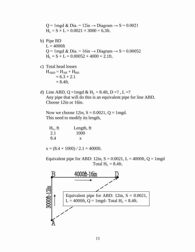
1. Line ABD

2 pipes in series (AB & BD)

Added head losses.

Assume Q = 1mgd.

a) Pipe AB

L = 3000ft

13

Q = 1mgd & Dia. = 12in → Diagram → S = 0.0021

HL = S × L = 0.0021 × 3000 = 6.3ft.

b) Pipe BD

L = 4000ft

Q = 1mgd & Dia. = 16in → Diagram → S = 0.00052

HL = S × L = 0.00052 × 4000 = 2.1ft.

c) Total head losses

HABD = HAB + HBD

= 6.3 + 2.1

= 8.4ft.

d) Line ABD, Q =1mgd & HL = 8.4ft, D =? , L =?

Any pipe that will do this is an equivalent pipe for line ABD.

Choose 12in or 16in.

Now we choose 12in, S = 0.0021, Q = 1mgd.

This need to modify its length,

HL, ft Length, ft

2.1 1000

8.4 x

x = (8.4 × 1000) / 2.1 = 4000ft.

Equivalent pipe for ABD: 12in, S = 0.0021, L = 4000ft, Q = 1mgd

Total HL = 8.4ft.

Equivalent pipe for ABD: 12in, S = 0.0021,

L = 4000ft, Q = 1mgd- Total HL = 8.4ft.

14

2. Line ACD

2 pipes in series (AC & CD)

Added head losses.

Assume Q = 0.5mgd.

a) Pipe AC

L = 4000ft

Q = 0.5mgd & Dia. = 10in → Diagram → S = 0.00142 = 1.42‰

HL = S × L = 0.00142 × 4000 = 5.7ft.

b) Pipe CD

L = 3000ft

Q = 0.5mgd & Dia. = 8in → Diagram → S = 0.0042 = 4.2‰

HL = S × L = 0.0042 × 3000 = 12.6ft.

c) Total head losses

HACD = HAC + HCD

= 5.7 + 12.6

= 18.3ft.

d) Line ACD, Q =0.5mgd & HL = 18.3ft

Any pipe that will do this is an equivalent pipe for line ABD.

Choose 10in or 8in.

Now we choose 8in, S = 0.0042, Q = 0.5mgd.

This need to modify its length,

HL, ft Length, ft

4.2 1000

18.3 x

x = (18.3 × 1000) / 4.2 = 4360ft.

Equivalent pipe for ABD: 8in, S = 0.0042, L = 4360ft, Q = 0.5mgd

Total HL = 18.3ft.

15

3. Equivalent line AD, choose HL = 8.4ft = HABD = HACD

What are the required parameters?

ABD & ACD in parallel with a given H

Q = QABD + QACD

Assume head loss already calculated for one of the lines

e.g. ABD, 12in, HL = 8.4ft.

a) Line ABD

L = 4000ft, 12in, HL = 8.4ft

Use 12in & S = HL / L = 8.4 / 4000 = 0.0021 → Diag.→ Q = 1mgd.

b) Line ACD

L = 4360ft, 8in, & HL = 8.4ft

Use 8in & S= HL/L = 8.4 / 4360 = 0.00192→Diag.→ Q = 0.33mgd.

c) Total discharge

Q = QABD + QACD

= 1 + 0.33

= 1.33mgd

d) Use equivalent pipe AD with Q = 1.33mgd, & HL = 8.4ft.

Assume equivalent pipe dia. = 14in.

Equivalent pipe for ABD: 8in, S = 0.0042,

L = 4360ft, Q = 0.5mgd, Total HL = 18.3ft.

16

14in & Q = 1.33 → Diag. → S = 1.68‰.

L = (8.4 * 1000) / 1.68

= 5000ft.

Equivalent pipe AD: 14in, L = 5000ft, HL = 8.4ft, Q = 1.33mgd.

See the Fig. below:

Eq. Pipe 5000ft -14in – 1.33mgd

17

3.Relaxation Method (Hardy Cross Method))طريقة هاردي كروس( The water distribution systems have sources ر(مصاد) & loads أحمال() . Such

systems either to design the original system or to expand the network.

Expansion means additional housing or commercial developments or

increased loads within existing area. Also prediction of required pressures in

the system is important.

Basic requirements:

1. Satisfy continuity, flow into & out each junction must be equal.

2. The head loss between any two junctions must be same.

3. The flow & head loss must be related by velocity-head loss equation.

The solution can be done by a trial & error hand computation. Now the

solution made by computers.

Theory of Hand computation)حساب اليذ(: How to find the velocity-head loss equation? Flows in the network is found

to be related by,

∑ hLc = hL-AB + hL-BC = ∑ K Qcn

∑ hLcc = ∑ K Qccn

Q1

Q2

Q3

Q4

Q1 = Q2+Q3+Q4

18

∑ hLc = ∑ hLcc & ∑ K Qcn = ∑ K Qcc

n

Where:

hLc = clockwise headloss

hLcc = counterclockwise headloss

Qc = clockwise discharge

Qcc = counterclockwise discharge

If clockwise head loss, hLc > hLcc by ∆Q

∑ K (Qc – ∆Q)n = ∑ K ( Qcc + ∆Q)

n

Expanding the summation & take only two terms,

∑ K (Qcn – nQc

n-1 ∆Q) = ∑ K (Qcc

n + nQcc

n-1 ∆Q)

(∑ n K Qcn-1

+ ∑ n K Qccn-1

) ∆Q = ∑ K Qcn - ∑ K Qcc

n

∆Q = (∑ K Qcn - ∑ K Qcc

n) / (∑ n K Qc

n-1 + ∑ n K Qcc

n-1)

If ∆Q = + → too much flow in clockwise → add ∆Q to counterclockwise

flows & subtract it from clockwise

flows.

The Darcy-Weisbach equation is used for computing the head loss,

hƒ = ƒ (L / D) (V2 / 2g)

= 8(ƒ L / gD5 π

2) Q

2

= KQ2

Where: K = 8(ƒ L / gD5 π

2)

Example(4):

For the given source & loads shown in Fig.A, how will the flow be

distributed in the simple network, and what will be the pressures at the load

points if the pressure at the source is 60 psi? Assume horizontal pipes &

ƒ=0.012 for all pipes. Diameter & length of each pipe is indicated in the Fig.

19

Fig. A

Solution:

Calculate head loss, K value for each pipe in the network using the

following equation,

K = 8(ƒ L / gD5 π

2)

For pipe (1000ft, & 24in):

00944.022.32

1000012.08

25

K

Fig. B shows the network with the head loss, K value for each pipe.

20

Fig. C shows the network with assumed flows:

Make the following tables:

Loop ABD

Pipe hƒ = K Q2 2KQ

AB 0.00944 × 100 = + 0.944 2 × 0.00944 × 10 = 0.189

AD 1.059 × 25 = - 26.475 2 × 1.059 × 5 = 10.590

BD 0 0

∑ - 25.531 10.779

∆Q = -25.531 /10.779

= - 2.40cfs.

21

Loop BCDE

Pipe hƒ = K Q2 2KQ

BC + 30.21 6.042

BD 0 0

CE 0 0

DE - 7.55 3.02

∑ + 22.66 9.062

∆Q = 22.66 /9.062

= 2.50cfs.

The corrections obtained in the table are applied to the two loops, and the

pipe discharges are shown in Fig. D.

Now the 1st iteration (cycle) is finished.

Use the new discharges (of 1st cycle) and do 2

nd cycle.

Loop ABD

Pipe hƒ = K Q2 2KQ

AB

AD

BD

∑

∆Q =

22

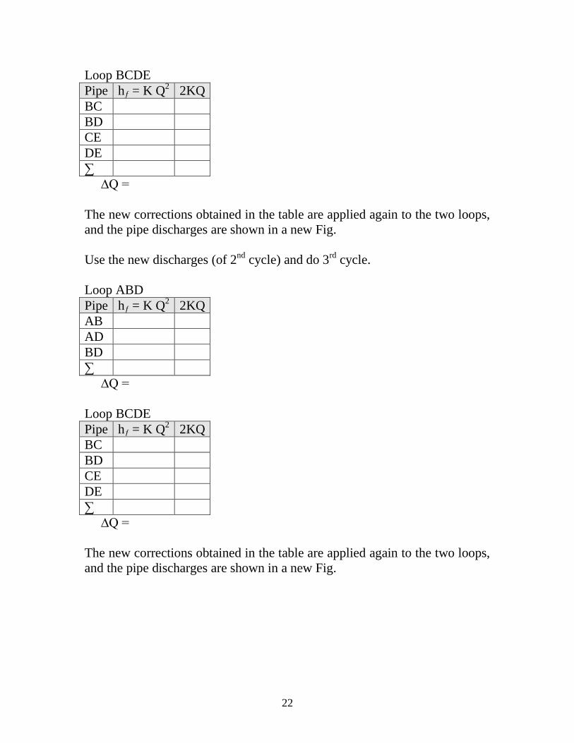
Loop BCDE

Pipe hƒ = K Q2 2KQ

BC

BD

CE

DE

∑

∆Q =

The new corrections obtained in the table are applied again to the two loops,

and the pipe discharges are shown in a new Fig.

Use the new discharges (of 2nd

cycle) and do 3rd

cycle.

Loop ABD

Pipe hƒ = K Q2 2KQ

AB

AD

BD

∑

∆Q =

Loop BCDE

Pipe hƒ = K Q2 2KQ

BC

BD

CE

DE

∑

∆Q =

The new corrections obtained in the table are applied again to the two loops,

and the pipe discharges are shown in a new Fig.

23

The final distribution of flow is obtained as shown in Fig. F.

The pressures at the load points are calculated as follows,

22

BCBCABABAC QKQKPP

= 60psi × (144psf/psi) – 62.4[0.00944 × (11.4)2 + 0.3021 × 9

2]

= 8640psf – 1603psf

= 7037psf

= 48.9psi

228640 DEDEADADE QKQKP

= 8640 – 62.4[1.059 × (3.5)2 + 0.3021 × 6

2]

= 7105psf

= 49.3psi.

Now we used this method for analysis a network, how we can use this

method for design.

Computer programming

Computer is used for detailed computations that can not practical to perform

by hand. Many programs are available e.g. WATER CAD, Pipe++, HC6,

EPANET & Pipe-Pro.

References:

- Fair, G. M., et al, 1968 “Elements of Water Supply & Wastewater Disposal”. - Roberson, J.A., et al, “Hydraulic Engineering”, 2nd Ed, John Wiley & Sons.

Inc., New York.

Documents

Analysis Methods for Water Distribution Systems-3rd Class