Embed Size (px)
Citation preview

Analysis by Meshless Local Petrov-Galerkin Method of
Material Discontinuities, Pull-in Instability in MEMS,
Vibrations of Cracked Beams, and Finite Deformations
of Rubberlike Materials
Maurizio Porfiri
Dissertation submitted to the Faculty of theVirginia Polytechnic Institute and State University
in partial fulfillment of the requirements for the degree of
Doctor of Philosophyin
Engineering Mechanics
Prof. Romesh C. Batra, ChairProf. Edmund G. Henneke
Prof. Michael W. HyerProf. Liviu Librescu
Prof. Douglas K. Lindner
April 27, 2006Blacksburg, Virginia
Keywords: MLPG method, MEMS, Vibrations,Rubberlike Materials, Discontinuities
Copyright 2006, Maurizio Porfiri

Analysis by Meshless Local Petrov-Galerkin Method of
Material Discontinuities, Pull-in Instability in MEMS,
Vibrations of Cracked Beams, and Finite Deformations
of Rubberlike Materials
Maurizio Porfiri
(Abstract)
The Meshless Local Petrov-Galerkin (MLPG) method has been employed to analyze the
following linear and nonlinear solid mechanics problems: free and forced vibrations of a
segmented bar and a cracked beam, pull-in instability of an electrostatically actuated mi-
crobeam, and plane strain deformations of incompressible hyperelastic materials. The Mov-
ing Least Squares (MLS) approximation is used to generate basis functions for the trial
solution, and for the test functions. Local symmetric weak formulations are derived, and
the displacement boundary conditions are enforced by the method of Lagrange multipliers.
Three different techniques are employed to enforce continuity conditions at the material in-
terfaces: Lagrange multipliers, jump functions, and MLS basis functions with discontinuous
derivatives. For the electromechanical problem, the pull-in voltage and the corresponding
deflection are extracted by combining the MLPG method with the displacement iteration
pull-in extraction algorithm. The analysis of large deformations of incompressible hypere-
lastic materials is performed by using a mixed pressure-displacement formulation. For every
problem studied, computed results are found to compare well with those obtained either
analytically or by the Finite Element Method (FEM). For the same accuracy, the MLPG
method requires fewer nodes but more CPU time than the FEM.

Acknowledgments
I wish to first and foremost acknowledge my advisor Dr. Romesh C. Batra. Without his
guidance, advice and encouragement this work would not have come to existence. I would like
to express my deep gratitude to my parents, my sister and all my late grandparents who have
always supported me, believed in me and covered me with love during all my studies. Next,
I would like to thank Dr. Edmund G. Henneke, my other committee members, Dr. Michael
W. Hyer, Dr. Liviu Librescu and Dr. Douglas K. Lindner, and the entire Department of
Engineering Science and Mechanics that gave me the chance to complete my studies in this
wonderful country, where I will hopefully find my way as a researcher. This dissertation
would not be complete without the unique collaboration over the past years with my friend
and colleague Davide Spinello. I also would like to express my gratitude to Dr. Daniel J.
Stilwell and the entire Autonomous Systems and Control Laboratory for hosting me as a
Post-Doctoral Fellow in the last year. I want to thank all my international friends, Alis, Bin,
Courtney, Farid, Gray, Hanif, Jan, Javier, Najm, Nawazish, Omid, Sibel and Umut for the
great friendship they always demonstrated with me. And finally, I would like to thank my
wife Maria for her endless support and help during these sometimes difficult years.
This work was partially supported by the Office of Naval Research grant N-00014-98-1-0300
to Virginia Polytechnic Institute and State University (VPI&SU), and the AFoSR MURI
grant to Georgia Tech that awarded a subcontract to VPI&SU. Views expressed in this
dissertation are those of the author and not of the funding agency.

Contents
1 Introduction 1
2 Free and Forced Vibrations of a Segmented Bar 3
2.1 Introduction . . . . . . . . . . . . . . . . . . . . . . . . . . . . . . . . . . . . 3
2.2 Modified MLS basis functions with discontinuous derivatives . . . . . . . . . 4
2.3 Governing equations . . . . . . . . . . . . . . . . . . . . . . . . . . . . . . . 6
2.4 MLPG6 weak and semidiscrete formulations . . . . . . . . . . . . . . . . . . 7
2.4.1 Discontinuity modeled by a jump function . . . . . . . . . . . . . . . 7
2.4.2 Discontinuity modeled by modified MLS basis functions with discon-
tinuous derivative . . . . . . . . . . . . . . . . . . . . . . . . . . . . . 10
2.4.3 Continuity of the displacement at the interface modeled by a Lagrange
multiplier . . . . . . . . . . . . . . . . . . . . . . . . . . . . . . . . . 11
2.4.4 Time integration scheme . . . . . . . . . . . . . . . . . . . . . . . . . 14
2.4.5 Numerical evaluation of domain integrals . . . . . . . . . . . . . . . . 15
2.5 Numerical results and comparisons . . . . . . . . . . . . . . . . . . . . . . . 15
2.5.1 Values of parameters . . . . . . . . . . . . . . . . . . . . . . . . . . . 15
2.5.2 Convergence analysis . . . . . . . . . . . . . . . . . . . . . . . . . . . 16
2.5.3 Forced vibrations . . . . . . . . . . . . . . . . . . . . . . . . . . . . . 18
2.6 Conclusions . . . . . . . . . . . . . . . . . . . . . . . . . . . . . . . . . . . . 20
3 Pull-in Instability in Electrically Actuated Narrow Microbeams 35
3.1 Introduction . . . . . . . . . . . . . . . . . . . . . . . . . . . . . . . . . . . . 35
iv

3.2 Model development . . . . . . . . . . . . . . . . . . . . . . . . . . . . . . . . 38
3.2.1 Governing equation for mechanical deformations . . . . . . . . . . . . 39
3.2.2 Distributed force due to electric field . . . . . . . . . . . . . . . . . . 39
3.2.3 Dimensionless governing equations . . . . . . . . . . . . . . . . . . . 40
3.2.4 Weak formulation . . . . . . . . . . . . . . . . . . . . . . . . . . . . . 41
3.3 Computation of the electric force field . . . . . . . . . . . . . . . . . . . . . . 42
3.3.1 Empirical formula for the capacitance . . . . . . . . . . . . . . . . . . 42
3.3.2 Validation of the capacitance estimate . . . . . . . . . . . . . . . . . 43
3.4 One-degree-of-freedom model . . . . . . . . . . . . . . . . . . . . . . . . . . 43
3.5 Numerical methods . . . . . . . . . . . . . . . . . . . . . . . . . . . . . . . . 46
3.5.1 Discrete nonlinear formulation . . . . . . . . . . . . . . . . . . . . . . 46
3.5.2 DIPIE algorithm . . . . . . . . . . . . . . . . . . . . . . . . . . . . . 48
3.6 Results and comparisons . . . . . . . . . . . . . . . . . . . . . . . . . . . . . 49
3.7 Conclusions . . . . . . . . . . . . . . . . . . . . . . . . . . . . . . . . . . . . 54
4 Vibrations of Cracked Euler-Bernoulli Beams 66
4.1 Introduction . . . . . . . . . . . . . . . . . . . . . . . . . . . . . . . . . . . . 66
4.2 Vibrations of a multiply cracked beam . . . . . . . . . . . . . . . . . . . . . 69
4.2.1 Governing equations . . . . . . . . . . . . . . . . . . . . . . . . . . . 69
4.2.2 Semi-discrete formulation . . . . . . . . . . . . . . . . . . . . . . . . 70
4.2.3 Inf-sup test . . . . . . . . . . . . . . . . . . . . . . . . . . . . . . . . 74
4.2.4 Modal analysis . . . . . . . . . . . . . . . . . . . . . . . . . . . . . . 76
4.2.5 Free motion . . . . . . . . . . . . . . . . . . . . . . . . . . . . . . . . 77
4.3 Effects of crack opening and closing . . . . . . . . . . . . . . . . . . . . . . . 78
4.4 Computation and discussion of results . . . . . . . . . . . . . . . . . . . . . 80
4.4.1 Convergence analysis . . . . . . . . . . . . . . . . . . . . . . . . . . . 82
4.4.2 Variations of weight functions radii . . . . . . . . . . . . . . . . . . . 83
v

4.4.3 Transient analysis for a breathing crack . . . . . . . . . . . . . . . . . 84
4.4.4 Remarks . . . . . . . . . . . . . . . . . . . . . . . . . . . . . . . . . . 85
4.5 Conclusions . . . . . . . . . . . . . . . . . . . . . . . . . . . . . . . . . . . . 86
5 Analysis of Rubber-like Materials 96
5.1 Introduction . . . . . . . . . . . . . . . . . . . . . . . . . . . . . . . . . . . . 96
5.2 Application of the MLPG method to non-linear elastic problems . . . . . . . 98
5.2.1 Local weak formulation . . . . . . . . . . . . . . . . . . . . . . . . . . 98
5.2.2 Total Lagrangian mixed formulation . . . . . . . . . . . . . . . . . . 99
5.2.3 Discrete formulation . . . . . . . . . . . . . . . . . . . . . . . . . . . 102
5.3 Computation and discussion of results . . . . . . . . . . . . . . . . . . . . . 103
5.3.1 Linear elastic problem for a cantilever . . . . . . . . . . . . . . . . . . 104
5.3.2 Uniform extension . . . . . . . . . . . . . . . . . . . . . . . . . . . . 104
5.3.3 Uniform shear . . . . . . . . . . . . . . . . . . . . . . . . . . . . . . . 105
5.3.4 Nonuniform extension . . . . . . . . . . . . . . . . . . . . . . . . . . 105
5.3.5 Nonuniform shear . . . . . . . . . . . . . . . . . . . . . . . . . . . . . 106
5.3.6 Crack problem . . . . . . . . . . . . . . . . . . . . . . . . . . . . . . 106
5.3.7 Remarks . . . . . . . . . . . . . . . . . . . . . . . . . . . . . . . . . . 108
5.4 Conclusions . . . . . . . . . . . . . . . . . . . . . . . . . . . . . . . . . . . . 108
6 Contributions 121
Bibliography 123
A MLS and GMLS approximations 132
A.1 Moving Least Squares (MLS) basis functions . . . . . . . . . . . . . . . . . . 132
A.2 Generalized Moving Least Squares (GMLS) basis functions . . . . . . . . . . 135
B Closed-form expressions for free and forced vibrations of the segmented
bar in Chapter 2 140
vi

B.1 Free vibrations . . . . . . . . . . . . . . . . . . . . . . . . . . . . . . . . . . 140
B.2 Forced vibrations . . . . . . . . . . . . . . . . . . . . . . . . . . . . . . . . . 141
C Method of moments 144
D Constitutive relations for hyperelastic and Mooney-Rivlin materials 146
Vita 150
vii

List of Figures
2.1 Modified MLS basis functions for nodes 1 through 6 obtained with m = 2 and
ri = 3L/ (N − 1). . . . . . . . . . . . . . . . . . . . . . . . . . . . . . . . . . 22
2.2 Schematic sketch of the problem studied. . . . . . . . . . . . . . . . . . . . . 23
2.3 Plot of the time-dependent axial traction applied at x = 0. . . . . . . . . . . 23
2.4 Plots of the jump function κ(
x−arJ
), and its derivative. . . . . . . . . . . . . 24
2.5 Subdomain ΩiS of node xi, and integration subregions obtained by the inter-
section of ΩiS with supports of domains of influence of neighboring nodes. . . 24
2.6 (a) Relative L2 error norm and, (b) relative H1 error norm for static defor-
mations under uniformly distributed load along the length of the bar. . . . . 25
2.7 (a) Axial displacement gradient near the material interface for a static de-
formation, and the percentage error in the derivative of the solution for the
uniformly distributed load, P/L, obtained with (b) the MLS basis functions
without treatment of the material discontinuity; (c) the MLS basis functions
with the three methods of treating the material discontinuity. . . . . . . . . 26
2.8 Relative L2 and H1 error norms for the first three mode shapes. . . . . . . . 27
2.9 First three mode shapes of the segmented bar. . . . . . . . . . . . . . . . . . 28
2.10 Relative error in the estimation of the first two natural frequencies. . . . . . 29
2.11 Snapshots of the traveling stress wave at (a) t = ac1
+ 3T4
, and (b) t = τ + 2T . 30
2.12 Snapshots of the displacement wave at (a) t = ac1
+ 3T4
, and (b) t = τ + 2T . . 31
viii

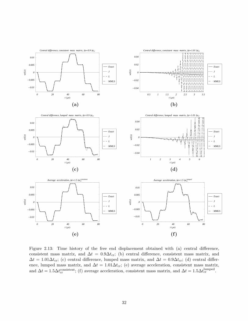
2.13 Time history of the free end displacement obtained with (a) central dif-
ference, consistent mass matrix, and ∆t = 0.9∆tcr; (b) central difference,
consistent mass matrix, and ∆t = 1.01∆tcr; (c) central difference, lumped
mass matrix, and ∆t = 0.9∆tcr; (d) central difference, lumped mass ma-
trix, and ∆t = 1.01∆tcr; (e) average acceleration, consistent mass matrix,
and ∆t = 1.5∆tconsistentcr ; (f) average acceleration, consistent mass matrix, and
∆t = 1.5∆tlumpedcr . . . . . . . . . . . . . . . . . . . . . . . . . . . . . . . . . . 32
2.14 Time history of the jump in the axial stress at the interface using (a) the
special jump function, (b) the Lagrange multiplier, and (c) the modified MLS
basis functions with discontinuous derivatives. . . . . . . . . . . . . . . . . . 33
2.15 At two different times, effect of the time step size on the L2 relative error
norm in the axial displacement. . . . . . . . . . . . . . . . . . . . . . . . . . 34
3.1 Electrostatically actuated clamped-clamped microbeam. . . . . . . . . . . . . 56
3.2 Electrostatically actuated cantilever microbeam. . . . . . . . . . . . . . . . . 56
3.3 Side view of the clamped-clamped microbeam. . . . . . . . . . . . . . . . . . 57
3.4 Side view of the cantilever microbeam. . . . . . . . . . . . . . . . . . . . . . 57
3.5 Schematic view of the beam cross section with grounded electrode . . . . . . 58
3.6 A system of auxiliary conductors for computing the electrostatic capacitance. 58
3.7 Taking the capacitance computed with the method of moments as reference,
comparison of the error in the capacitance per unit length for a narrow mi-
crobeam obtained with different methods: (a) β = 0.2; (b) β = 2. . . . . . . 59
3.8 Schematics of the 3D FE mesh used for simulations of the clamped-clamped
beam by ANSYS. The domain in light grey (discretized with tetrahedral ele-
ments) is the dielectric, the one in dark grey (discretized with brick elements)
is the microbeam. . . . . . . . . . . . . . . . . . . . . . . . . . . . . . . . . . 60
3.9 Plots of the maximum displacement versus the applied voltage for the clamped-
clamped microbeam problem under different initial states of stress. Results
from all models are reported up to their predicted pull-in instability. (a)
σ0 = 100MPa; (b) σ0 = 0MPa; (c) σ0 = −100MPa. . . . . . . . . . . . . . 61
3.10 Plot of the maximum displacement versus the applied voltage for the cantilever
microbeam of case (1), Table 3.2. Results from all models are reported up to
their predicted pull-in instability. . . . . . . . . . . . . . . . . . . . . . . . . 62
ix

3.11 Deformed shapes of microbeams just prior to the pull-in voltage. Dimensions
along the x- and the y-axes are in µm; (a) cantilever microbeam of case (2),
Table 3.2; (b) clamped-clamped microbeam with σ0 = 0MPa. . . . . . . . . 63
3.12 For the cantilever beam identified as case (2) in Table 3.2, comparison of the
nondimensional pull-in voltage µ vs. 1/β computed from the present 1 d.o.f.
model with those from Osterberg and Senturia (1997), Abdel-Rahman, Younis
and Nayfeh (2002), and Kuang and Chen (2004). . . . . . . . . . . . . . . . 64
3.13 For the clamped-clamped microbeam of Table 3.2 with σ0 = 0MPa, com-
parison of the non-dimensional pull-in voltage µ vs. 1/β computed from the
present 1 d.o.f. model with those from Osterberg and Senturia (1997), Abdel-
Rahman, Younis and Nayfeh (2002), and Kuang and Chen (2004). . . . . . . 64
3.14 For the cantilever beam identified as case (2) in Table 3.2, comparison of the
maximum pull-in non-dimensional deflection ‖w‖∞ vs. 1/β computed from
the present 1 d.o.f. model with those from Osterberg and Senturia (1997),
Abdel-Rahman, Younis and Nayfeh (2002), and Kuang and Chen (2004). . . 65
3.15 For the clamped-clamped microbeam described in Table 3.2 with σ0 = 0MPa,
comparison of the maximum pull-in non-dimensional deflection ‖w‖∞ vs. 1/β
computed from the present 1 d.o.f. model, with those from Osterberg and
Senturia (1997), Abdel-Rahman, Younis and Nayfeh (2002), and Kuang and
Chen (2004). . . . . . . . . . . . . . . . . . . . . . . . . . . . . . . . . . . . 65
4.1 Sketch of a cracked beam and of its lumped flexibility model. . . . . . . . . . 89
4.2 For a uniformly loaded beam, convergence of the error norms with a decrease
in the nodal spacing or an increase in the number of uniformly distributed
nodes. . . . . . . . . . . . . . . . . . . . . . . . . . . . . . . . . . . . . . . . 90
4.3 Convergence rates of the first three natural frequencies. . . . . . . . . . . . . 90
4.4 Convergence rates of the three lowest modes in L2 norm. . . . . . . . . . . . 91
4.5 Convergence rates of the three lowest modes in H1 norm. . . . . . . . . . . . 91
4.6 Convergence rates of the three lowest modes in H2 norm. . . . . . . . . . . . 92
4.7 For uniform loading and for 4+4 nodes, convergence with the weight functions
radii. . . . . . . . . . . . . . . . . . . . . . . . . . . . . . . . . . . . . . . . . 92
4.8 Dependence of the relative error of the four lowest resonance frequencies for
4 + 4 nodes upon the weight functions radii. . . . . . . . . . . . . . . . . . . 93
x

4.9 Exact (solid), approximate (triangles) and experimental (circles) lowest fre-
quency ratio with different crack severities. . . . . . . . . . . . . . . . . . . . 94
4.10 Time evolution of the deflection field at the crack station: breathing crack with
25 mode shapes (solid), breathing crack with the MLPG method (triangles),
and exact solution for the intact beam (dashed). . . . . . . . . . . . . . . . . 95
4.11 Time evolution of the change of rotations at the crack station: breathing crack
with 25 mode shapes (solid), and breathing crack with the proposed method
(triangles). . . . . . . . . . . . . . . . . . . . . . . . . . . . . . . . . . . . . . 95
5.1 Geometry and locations of primary nodes for the sample problem studied. . 110
5.2 Uniform extension of a plate: undeformed configuration (shaded), exact solu-
tion (empty circles), MLPG solution (dots). . . . . . . . . . . . . . . . . . . 111
5.3 Uniform shear of a plate: undeformed configuration (shaded), exact solution
(empty circles), MLPG solution (dots). . . . . . . . . . . . . . . . . . . . . . 112
5.4 Nonuniform extension of a plate: undeformed configuration (shaded), exact
solution (empty circles), MLPG solution (dots). . . . . . . . . . . . . . . . . 113
5.5 Nonuniform shear of a plate: undeformed configuration (shaded), exact solu-
tion (empty circles), MLPG solution (dots). . . . . . . . . . . . . . . . . . . 114
5.6 Geometry of a cracked plate loaded in mode-I. . . . . . . . . . . . . . . . . . 115
5.7 Locations of primary (filled circles) and secondary (empty circles) nodes in
the quarter of a cracked plate. . . . . . . . . . . . . . . . . . . . . . . . . . 116
5.8 Undeformed (solid line), deformed (dotted) shape of the cracked plate, and
final locations of primary (filled circles) and secondary (empty circles) nodes. 117
5.9 J-integral from the linear analysis (solid line), and J-integral from the nonlin-
ear analysis (empty circles and dashed fitting curve) versus applied nominal
surface traction. . . . . . . . . . . . . . . . . . . . . . . . . . . . . . . . . . . 118
5.10 Crack opening displacement computed using the MLPG formulation (dia-
mond), and ANSYS FE code (empty circles) versus applied nominal surface
traction. . . . . . . . . . . . . . . . . . . . . . . . . . . . . . . . . . . . . . . 119
5.11 Normalized first Piola Kirchhoff stress in the neighborhood of the crack tip
for different values of the applied nominal surface traction σ0. . . . . . . . . 120
5.12 Normalized Cauchy stress in the neighborhood of the crack tip for different
values of the applied nominal surface traction σ0. . . . . . . . . . . . . . . . 120
xi

A.1 Sketch of the GMLS approximation. . . . . . . . . . . . . . . . . . . . . . . . 139
xii
List of Tables
2.1 Critical time step, ∆tcr [µs], for different methods of accounting for material
discontinuity. . . . . . . . . . . . . . . . . . . . . . . . . . . . . . . . . . . . 19
3.1 Comparison between the capacitances per unit length computed by the Method
of Moments (MoM) with those from (3.9) by substituting in it the expression
(3.21) for the fringing field, and from three formulas available in the literature. 44
3.2 Geometric and material parameters for the problems studied. For the can-
tilever beam problem, case (1) refers to the geometry analyzed herein with
ANSYS, while case (2) to the problem analyzed in Pamidighantam, Puers,
Baert and Tilmans (2002). . . . . . . . . . . . . . . . . . . . . . . . . . . . . 50
3.3 Comparison of pull-in voltages, VPI , and pull-in deflections infinity norm,
‖wPI‖∞, of the clamped-clamped microbeam obtained from different models,
different methods, and with different values of the initial stress, σ0; (a) σ0 =
100MPa, (b) σ0 = 0, and (c) σ0 = −100MPa. The MLPG and the FE refer
to solutions of the one-dimensional boundary-value problem with the MLPG
and the FE methods respectively. . . . . . . . . . . . . . . . . . . . . . . . . 52
3.4 Comparison of pull-in voltages and pull-in deflections of the cantilever mi-
crobeam obtained from different models and different methods. The MLPG
and the FE refer to solutions of the one-dimensional boundary-value problem
with the MLPG and the FE methods respectively. . . . . . . . . . . . . . . . 53
4.1 Comparison of the MLPG method and the FEM for vibrations of a cracked
beam. . . . . . . . . . . . . . . . . . . . . . . . . . . . . . . . . . . . . . . . 88
5.1 For a cantilever beam, percentage error in the tip deflection computed with
mixed and pure displacement MLPG formulations. . . . . . . . . . . . . . . 105
xiii

Chapter 1
Introduction
Recently, considerable research in computational mechanics has been devoted to the devel-
opment of meshless methods, that lessen the difficulty of meshing and remeshing the entire
structure, by only adding or deleting nodes at suitable locations (see, e.g., Liu (2003) for
a thorough review of meshless methods). Meshless methods may also alleviate some other
problems associated with the Finite Element Method (FEM), such as locking and element
distortion. In many applications, they provide smooth, and accurate approximate solutions
with a reduced number of nodes.
During the last two decades, several meshless methods for seeking approximate solutions of
partial differential equations have been proposed; these include the element-free Galerkin
(Belytschko, Lu and Gu (1994)), hp-clouds (Duarte and Oden (1996)), the reproducing ker-
nel particle (Liu, Jun, Adee and Belytschko (1995), Liu, Jun and Zhang (1995), Chen, Pan
and Wu (1997)), the smoothed particles hydrodynamics (SPH) (Lucy (1977)), the diffuse ele-
ment (Nayroles, Touzot and Villon (1992)), the partition of unity finite element (Melenk and
Babuska (1996)), the natural element (Sukumar, Moran and Belytschko (1998)), meshless
Galerkin using radial basis functions (Wendland (1995)), the meshless local Petrov-Galerkin
(MLPG) (Atluri and Zhu (1998)), the modified smoothed particle hydrodynamics (MSPH)
(Zhang and Batra (2004)), and the collocation method with radial basis functions (Ferreira,
Batra, Roque, Qian and Martins (2005)). All of these methods, except for the MLPG, the
SPH, the MSPH, and the collocation method are not truly meshless since the use of shadow
elements is required for evaluating integrals appearing in the governing weak formulations
(see, e.g., Atluri and Shen (2002)). The MLPG method has been successfully applied to
several structural problems: static linear plane elasticity (Atluri and Zhu (1998)); vibrations
of elastic planar bodies (Gu and Liu (2001a)); static analysis of thin plates (Gu and Liu
(2001b)); static analysis of beams (Atluri, Cho and Kim (1999), Raju and Phillips (2003));
vibrations of cracked beams (Andreaus, Batra and Porfiri (2005)); static and dynamic prob-
lems for functionally graded materials (Qian, Batra and Chen (2004a,b)) and (Qian and
1

Batra (2004)); static and dynamic problems for thick rectangular plates (Qian, Batra and
Chen (2003a,b); analysis of transient problems with material discontinuities (Batra, Por-
firi and Spinello (2006a)); heat conduction problems in multimaterial bodies (Batra, Porfiri
and Spinello (2004)) and analysis of microelectromechanical problems (Batra, Porfiri and
Spinello (2006b,c)). The MLPG method is based on local weak forms of governing equations
and employs meshless interpolations for both the trial and the test functions. The trial func-
tions are constructed by using the Moving Least Squares (MLS) (Lancaster and Salkauskas
(1981)) approximation and its enhanced versions proposed by Atluri, Chom and Kim (1999),
and Kim and Atulri (2000), or the radial basis functions (see, e.g., Kansa (1990)). These
approximations simply rely on the location of points or nodes in the body, rather than com-
plex meshes. In the Petrov-Galerkin formulation, test functions may be chosen from a space
different from the space of trial functions; in this way, depending upon the choice of the test
function, and the employment of a local symmetric or local asymmetric weak form, Atluri
and Shen (2002) proposed six variants, namely MLPG1, MLPG2,..., MLPG6, of the MLPG
method. In MLPG6, the local symmetric Bubnov-Galerkin formulation, the test function
for each subdomain is chosen to be the MLS basis function associated with a node. Another
relevant feature of the MLPG method is that, the domains of integration may either overlap
or their union may not equal the domain occupied by the body.
Thus the key ingredients of the MLPG method may be summarized as: local weak formula-
tion, MLS interpolation, Petrov-Galerkin projection, evaluation of domain integrals appear-
ing in the weak formulation, imposition of essential boundary conditions, and for transient
problems time-integration of the resulting ordinary differential equations.
2

Chapter 2
Free and Forced Vibrations of aSegmented Bar
2.1 Introduction
For a body made of two or more materials, the derivative of displacements in the direction
normal to the interface between two materials must be discontinuous in order for surface
tractions there to be continuous. For the analysis of linear elastostatic problems by the EFG
method, Cordes and Moran (1996) used the method of Lagrange multipliers, Krongauz and
Belytschko (1998) employed a special jump function at the line or the surface of discontinuity,
and Noguchi and Sachiko (2006) modified the Moving Least Square (MLS) basis functions
so that their derivative jumps at desired locations. Whereas a two-dimensional (2-D) static
problem was analyzed by Krongauz and Belytschko (1998), a 1-D static problem was scru-
tinized by Cordes and Moran (1996). Batra, Porfiri and Spinello (2004) have compared the
performance of two MLPG formulations in the analysis of a parabolic 1-D problem, i.e., the
axisymmetric transient heat conduction in a bimetallic disk with the material discontinuity
treated either by the method of Lagrange multipliers or the jump function. Note that no
waves propagate in a parabolic problem. However, waves propagate in a hyperbolic problem,
and may be reflected and refracted at the interface between the two materials.
In this chapter, we use the MLPG6 formulation, that is trial and test functions are chosen
from the same space generated by the Moving Least Squares (MLS) approximation. We
compare the performance of the three aforementioned techniques to account for material
discontinuities in the analysis of free, and forced vibrations of a segmented bar. As a sample
problem we consider a clamped-free bimaterial bar, although the approach is also suitable for
other boundary conditions. The essential (i.e. displacement) boundary condition is imposed
Material in this Chapter is part of the paper “Free and Forced Vibrations of a Segmented Bar by a MeshlessLocal Petrov-Galerkin (MLPG) Formulation,” accepted for publication in Computational Mechanics.
3

in all cases by introducing a Lagrange multiplier; this technique was used by Warlock,
Ching, Kapila and Batra (2002) and Batra and Wright (1986) to satisfy contact conditions
at a rough surface. Following the idea developed by Andreaus, Batra and Porfiri (2005) for a
beam, it is shown that the MLPG6 numerical solution is stable and optimal by showing that
the related mixed formulations satisfy the ellipticity and the inf-sup conditions (see Bathe
(1996)). Numerical results are compared with analytical and FE solutions. In particular, the
convergence with an increase in the number of nodes of the first two eigenfrequencies, first
three mode shapes, and a static solution are shown, revealing a monotonically decreasing
trend at a rate faster than that obtained with the FE method. The transient response to an
axial traction of finite duration applied at one end of the bar is shown to match very well
with the analytical solution of the problem.
The rest of the Chapter is organized as follows. In Section 2.2 we introduce the MLS
basis functions with discontinuous derivatives (Noguchi and Sachiko (2006)). Section 2.3
gives differential equations, and initial and boundary conditions for wave propagation in a
segmented elastic bar with one end clamped and the other free. Section 2.4 presents the
MLPG6 formulations for the method of Lagrange multipliers, the method of jump function,
and the method of MLS basis functions with discontinuous derivatives. In Section 2.4, we
also very briefly discuss the numerical evaluation of domain integrals, and the method used
to numerically integrate, with respect to time, the semidiscrete system of ordinary differ-
ential equations. Numerical results computed with the three methods of treating material
discontinuities are discussed in Section 2.5 where the convergence of the MLPG6 solution
for static deformations, and mode shapes is compared with that of the FE solution, and
the transient response to a time dependent axial traction is compared with the analytical
solution of the corresponding problem. Section 2.6 summarizes conclusions. The ordinary
MLS approximation may be found in Appendix A.1. Analytical solutions of the problem for
free, and forced vibrations of the segmented bar are given in the Appendices B.1 and B.2
respectively.
2.2 Modified MLS basis functions with discontinuous derivatives
Let a material interface be located at the point a ∈ (0, L) in the global domain Ω = [0, L].
Consider N scattered points x1, . . . , xN and let a node be located at x = a. Herein, we
derive a modified MLS approximation that allows for the reconstruction of a function w in Ω
whose derivative jumps at x = a. We refer to Appendix A.1 for a detailed explanation of the
ordinary MLS approximation. We denote by N1 and N2 the number of nodes whose location
xj satisfies the condition xj ≤ a, and xj > a respectively. Let Wj be the weight function of
the j-th node and rj be the radius of its support. Also, let n1 and n2 be the number of nodes
4

whose location xj satisfies the condition a− rN1 < xj ≤ a, and a < xj < a+ rN1 respectively.
In other words, n1 and n2 equal the number of nodes in the domain of influence of the weight
function WN1 associated with the interface node at xN1 = a, placed, respectively, to the left
and to the right of the interface. In order to modify the ordinary MLS basis functions in the
domain of influence of the weight function WN1 in such a way that all basis functions which
are nonzero at the interface are continuous but have discontinuous derivative, we consider
the following global approximation of the function w in the region (a− rN1 , a + rN1):
wh (x) =
pT
1 (x)b (x) , x ∈ (a− rN1 , a]
pT2 (x)b (x) , x ∈ (a, a + rN1)
, (2.1)
withpT
1 (x) =[1 x− a 0 (x− a)2 0 · · · (x− a)m−1 0
],
pT2 (x) =
[1 0 x− a 0 (x− a)2 · · · 0 (x− a)m−1
],
(2.2)
and
b (x) =[b0 (x) b1,1 (x) b2,1 (x) · · · b1,m−1 (x) b2,m−1 (x)
]. (2.3)
For example, for m = 2 one gets
wh (x) =
b0 (x) + (x− a) b1,1 (x) , x ≤ ab0 (x) + (x− a) b2,1 (x) , x > a
. (2.4)
The weighted discrete L2 error norm to be minimized is (see (A.5))
Jx (b) =
n1∑i=1
Wi (x)[pT
1 (xi)b (x)− wi
]2+
n1+n2∑i=n1+1
Wi (x)[pT
2 (xi)b (x)− wi
]2, (2.5)
for x ∈ (a− rN1 , a + rN1). By extremizing the functional J in (2.5) one obtains
A (x) = PTW (x)P, B (x) = PTW (x) . (2.6)
where
A (x) =n1∑i=1
Wi (x)p1 (xi)pT1 (xi) +
n1+n2∑i=n1+1
Wi (x)p2 (xi)pT2 (xi) ,
B (x) = [W1 (x)p1 (x1) , . . . , Wn1 (x)p1 (xn1) ,Wn1+1 (x)p2 (xn1+1) , . . . , Wn1+n2 (x)p2 (xn1+n2)].
(2.7)
Solving (2.6) for b we obtain
b (x) = A∗ (x)B (x) , (2.8)
where A∗ is the pseudoinverse of matrix A. Indeed, assuming that at every evaluation point x
there are at least m nonvanishing weight functions, for the null space of the (2m− 1× 2m− 1)
matrix A the following holds:
0 ≤ dim kerA ≤ m− 1. (2.9)
5

When dim kerA = 0, A is invertible, and its inverse and pseudoinverse coincide. However,
when dim kerA > 0, there are as many zero rows and columns in A as the number of
vanishing weight functions at x; in this case the nonzero entries of the pseudoinverse are
equal to the entries of the matrix obtained from A by deleting its zero rows and columns.
Note that the corresponding rows of the matrix B are also zero; therefore (2.8) states that
the related entries in the vector b are zero.
For 11 uniformly distributed nodes in the domain [0, L] with the interface between two
materials located at a = L/2 or at node 6, the modified MLS basis functions for nodes 1
through 6 are plotted in Figure 2.1, where we have set m = 2, ri = 3L/10, and two nodes
in the radius of support of each weight function. We emphasize that, in this approach, the
weight functions are not modified, while all basis functions in the domain of influence of the
weight function WN1 are modified due to the introduction of the discontinuous monomial
basis (2.2) in the region (a− rN1 , a + rN1) , which affects matrices A and B in the same
region, and therefore the MLS basis functions. Even though the weight functions in (2.5)
are non-negative, the basis functions may assume negative values. Also, a basis function is
non-zero at more than one node. It is clear that basis functions for nodes in the domain of
influence of the weight function W6 ( i.e., for nodes 4, 5, and 6), have discontinuous derivative
at node 6.
2.3 Governing equations
We study wave propagation in a segmented bar of length L with the left segment of length a
made of one material, and the right one of length L− a made of a different material (Figure
2.2); Ei and %i, i = 1, 2, are, respectively, Young’s modulus, and the volumetric mass density
of the material constituting the left, and the right parts. As an example problem, the right
end of the bar is clamped, and a time dependent axial traction p (t) is applied at the left
end. By assuming a uniform cross section, governing equations are
%1w1 (x, t)− E1w′′1(x, t) = 0, x ∈ (0, a) , t > 0, (2.10)
%2w2 (x, t)− E2w′′2(x, t) = 0, x ∈ (a, L) , t > 0, (2.11)
with boundary conditions
E1w′1 (0, t) = p (t) , (2.12)
w1 (a, t) = w2 (a, t) , (2.13)
E1w′1 (a, t) = E2w
′2 (a, t) , (2.14)
w2 (L, t) = 0. (2.15)
6

We assume homogeneous initial conditions
w1 (x, 0) = w2 (x, 0) = 0,
w1 (x, 0) = w2 (x, 0) = 0. (2.16)
Here, wi (x, t) is the longitudinal displacement of point x in the i− th segment of the bar; a
superimposed dot means partial differentiation with respect to time t, while a prime means
partial differentiation with respect to x. The global axial displacement field, w, is given by
w (x, t) =
w1 (x, t) , x ∈ (0, a)w2 (x, t) , x ∈ (a, L)
, (2.17)
and a similar notation will be adopted for the global volumetric mass density, and Young’s
modulus.
Equations (2.13) and (2.14) state the continuity of the displacement, and of the axial stress
at the interface. We note that the derivative w′ must be discontinuous at the interface to
guarantee the continuity of the axial stress.
In the forced vibration analysis, we will consider an axial traction applied at x = 0, shown
in Figure 2.3, and given by
p (t) = P sin
(πt
T
)[H (t)−H (t− T )] , (2.18)
where H is the Heaviside function, the dimension of P is force/area, and T measures the
finite duration of the applied traction.
2.4 MLPG6 weak and semidiscrete formulations
In this Section, the MLPG6 formulation of the boundary-value problem (2.10)-(2.15) is
derived. A Local Symmetric Augmented Weak Formulation (LSAWF) is stated for each
one of the three methods of treating material discontinuities. The projection of trial and
test functions on finite-dimensional basis functions leads to semidiscrete formulations of the
problem, or equivalently a system of ordinary differential equations in time. It is shown that
these mixed semidiscrete formulations are optimal, and stable in the sense that they satisfy
both the ellipticity, and the inf-sup (Babuska-Brezzi) conditions.
2.4.1 Discontinuity modeled by a jump function
Semidiscrete formulation
Let ΩiS ⊆ [0, L], i = 1, 2, . . . , N be a family of subdomains of the global domain such that
∪Ni=1Ω
iS = [0, L]. We introduce the following LSAWF of the problem on the i-th subdomain
7

ΩiS:
0 =
∫
ΩiS
%wwidx +
∫
ΩiS
Ew′w′idx (2.19)
−[(1− δL) Ew′wi + δL
(λLwi + λLw
)]∣∣∣Γi+
S
+ [(1− δ0) Ew′wi + δ0pwi]|Γi−S
.
Here, wi ∈ H1 (0, L) is a test function for w,
δy (x) :=
1, x = y0, x 6= y
, (2.20)
and Γi−S , Γi+
S are the left, and the right boundary points of the subdomain ΩiS. In order
to enforce the essential boundary condition (2.15), the Lagrange multiplier λL has been
introduced, and the scalar λL is the corresponding test function. We emphasize that the
natural boundary condition (2.12) has also been considered. The variational statement
(2.19) can be derived by extremizing the Action related to an augmented Lagrangian on the
set of isochronous motions following classical arguments, see, e.g., Mura and Koya (1992).
In order to capture the discontinuity in w′ at the interface we enrich the set of smooth MLS
basis functions ψ (x) with a special jump function κ (x). Therefore, we approximate the
axial displacement field by
wh (x, t) = ψT (x) w (t) + q (t)κ (x) , (2.21)
where the additional unknown q (t) represents the jump in the axial strain at time t and
w is comprised of nodal unknowns. The jump function κ (x) and its first derivative are
continuous in both segments of the bar, and its first derivative jumps at x = a in order to
ensure the continuity of the axial stress without affecting the continuity of the displacement
field. Following Krongauz and Belytschko (1998), we take
κ (x) =
1
6− 1
2
( |x− a|rJ
)+
1
2
( |x− a|rJ
)2
− 1
6
( |x− a|rJ
)3
,|x− a|
rJ
≤ 1
0,|x− a|
rJ
> 1
. (2.22)
The size of the support of κ (x) equals 2rJ and, as shown in Figure 2.4, the jump function
and its derivative go to zero smoothly as |x − a|/rJ → 0, while the derivative of κ(|x−a|
rJ
)
jumps from 1/2 at x = a− to −1/2 at x = a+.
In order to generate N + 2 equations for the N + 1 nodal unknowns
u (t) =[w (t) q (t)
]T, (2.23)
and the Lagrange multiplier λL, we consider the set of N + 2 independent test functions
Ψ (x) =[ψ1 (x) · · · ψN (x) κ (x)
]T, (2.24)
8
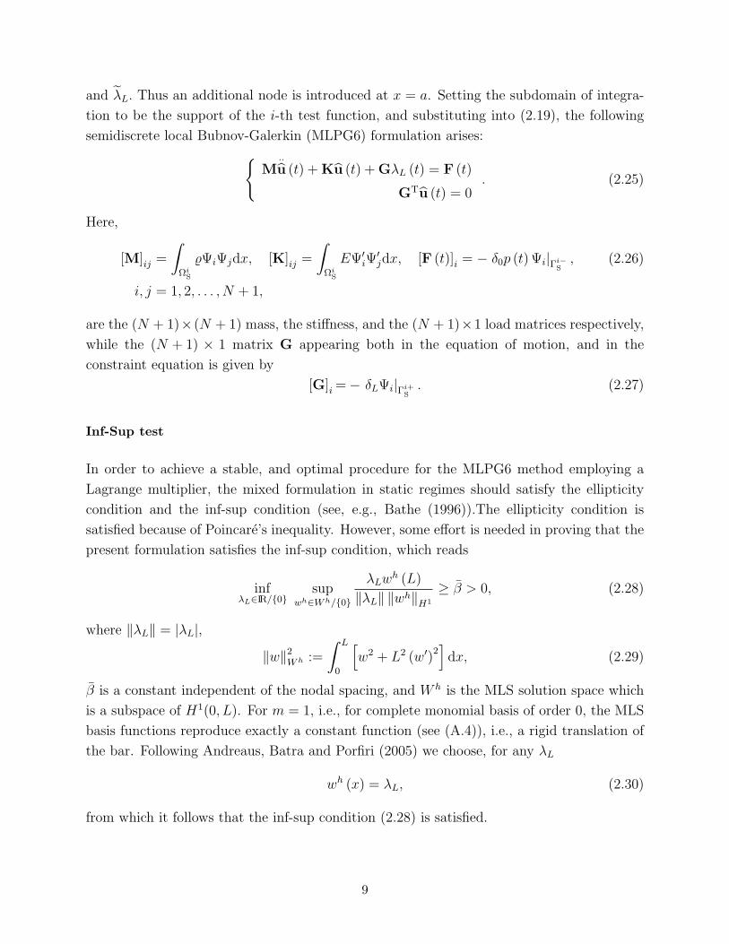
and λL. Thus an additional node is introduced at x = a. Setting the subdomain of integra-
tion to be the support of the i-th test function, and substituting into (2.19), the following
semidiscrete local Bubnov-Galerkin (MLPG6) formulation arises:
M
..
u (t) + Ku (t) + GλL (t) = F (t)
GTu (t) = 0. (2.25)
Here,
[M]ij =
∫
ΩiS
%ΨiΨjdx, [K]ij =
∫
ΩiS
EΨ′iΨ
′jdx, [F (t)]i = − δ0p (t) Ψi|Γi−
S, (2.26)
i, j = 1, 2, . . . , N + 1,
are the (N + 1)× (N + 1) mass, the stiffness, and the (N + 1)×1 load matrices respectively,
while the (N + 1) × 1 matrix G appearing both in the equation of motion, and in the
constraint equation is given by
[G]i =− δLΨi|Γi+S
. (2.27)
Inf-Sup test
In order to achieve a stable, and optimal procedure for the MLPG6 method employing a
Lagrange multiplier, the mixed formulation in static regimes should satisfy the ellipticity
condition and the inf-sup condition (see, e.g., Bathe (1996)).The ellipticity condition is
satisfied because of Poincare’s inequality. However, some effort is needed in proving that the
present formulation satisfies the inf-sup condition, which reads
infλL∈IR/0
supwh∈W h/0
λLwh (L)
‖λL‖ ‖wh‖H1
≥ β > 0, (2.28)
where ‖λL‖ = |λL|,‖w‖2
W h :=
∫ L
0
[w2 + L2 (w′)2
]dx, (2.29)
β is a constant independent of the nodal spacing, and W h is the MLS solution space which
is a subspace of H1(0, L). For m = 1, i.e., for complete monomial basis of order 0, the MLS
basis functions reproduce exactly a constant function (see (A.4)), i.e., a rigid translation of
the bar. Following Andreaus, Batra and Porfiri (2005) we choose, for any λL
wh (x) = λL, (2.30)
from which it follows that the inf-sup condition (2.28) is satisfied.
9

Reduced semidiscrete system of equations
The second equation in (2.25) provides a constraint for the unknown vector u. By properly
manipulating the system (2.25) we obtain a simpler formulation where the constraint is
automatically satisfied.
Let kerGT be the null space of G T; since the inf-sup condition holds, dim kerGT = N (see,
e.g., Bathe, 1996). Next, we introduce the N × (N + 1) matrix X whose rows constitute a
basis for kerGT, and the reduced N -vector of unknowns u:
u = XTu. (2.31)
It is clear that the constraint equation is automatically satisfied for every u ∈ IRN . Sub-
stituting (2.31) into (2.25)1, and premultiplying by X one obtains the following reduced
semidiscrete system of equations for u:
mu (t) + ku (t) = f (t) , (2.32)
where
m = XMXT, k = XKXT, f = XF. (2.33)
After solving for u, we obtain the complete vector of unknowns u by using (2.31).
2.4.2 Discontinuity modeled by modified MLS basis functions with discontinu-ous derivative
Let N nodes be located in the global domain [0, L] with a node placed at the interface x = a,
and let ϕ (x) be the set of MLS basis functions modified as in Section 2.2. The MLPG6
semidiscrete formulation is obtained in a similar way as for the method of jump function,
i.e. by substituting in the LSAWF (2.19) the approximation wh (x, t) = ϕT (x) w (t) for the
trial solution, by considering the basis function ϕi as test function for the i-th subdomain,
and by setting ΩiS equal to the support of ϕi. Therefore, the following N + 1 equations for
the N nodal unknowns w, and the Lagrange multiplier λL are obtained:
M..
w (t) + Kw (t) + GλL (t) = F (t) ,
GTw (t) = 0.(2.34)
The entries of the (N ×N) mass and stiffness matrices, of the N load vector, and of the
(N × 1) matrix G are given by
[M]ij =
∫
ΩiS
%ϕiϕjdx, [K]ij =
∫
ΩiS
Eϕ′iϕ′jdx, [F (t)]i = − δ0p (t) ϕi|Γi−
S, (2.35)
[G]i=− δLϕi|Γi+S
, i, j = 1, 2, . . . , N. (2.36)
10

It is easy to check (see Section 2.4.1) that the static form of the semidiscrete formulation
(2.34) is elliptic, and that it satisfies the inf-sup condition. Therefore, we can introduce the
reduced (N − 1)-vector of unknowns w:
w = XTw, (2.37)
where X is the (N − 1)×N matrix whose rows constitute a basis for kerGT. The constraint
represented by the second equation in (2.34) is then automatically satisfied; upon substitution
from (2.37) into the first equation in (2.34), and premultiplication by X one obtains a reduced
system of N − 1 equations for the N − 1 unknowns w formally analogous to (2.32).
2.4.3 Continuity of the displacement at the interface modeled by a Lagrangemultiplier
Semidiscrete formulation
Let xi ∈ [0, a] , i = 1, . . . , N1, and xi ∈ [a, L] , i = N1 + 1, . . . , N1 + N2 be two sets of
nodes such that xN1 ≡ xN1+1 = a, and
ΩiS1 ⊂ [0, a] , i = 1, . . . , N1; Ωk
S2 ⊂ [a, L] , k = N1+1, N1+2, . . . , N1+N2−1, N1+N2 =: N,
(2.38)
be the corresponding disjoint families of subdomains covering [0, a], and [a, L] respectively.
Following Cordes and Moran (1996), we consider the augmented variational statement
0 =
∫
ΩiS1
%1w1w1idx +
∫
ΩiS1
E1w′1w
′1idx +
∫
ΩkS2
%2w2w2kdx +
∫
ΩkS2
E2w′2w
′2kdx
−[(1− δa) E1w
′1w1i − δa
(λa w1i + λa w1
)]∣∣∣Γi+
S1
+ [(1− δ0) E1w′1w1i + δ0pw1i]|Γi−
S1
−[(1− δL) E2w
′2w2k + δL
(λL w2k + λL w2
)]∣∣∣Γk+
S2
+[(1− δa) E2w
′2w2k − δa
(λa w2k + λa w2
)]∣∣∣Γk−
S2
. (2.39)
Here, w1i, w2k, λa, and λL are test functions for the displacement fields, and the Lagrange
multipliers λa and λL introduced to enforce the continuity of the displacement at the interface
(2.13), and the essential boundary condition (2.15). In this approach, two problems are
separately formulated in the two homogenous parts of the bar; two overlapping nodes are
placed at the interface, and the two problems are connected by the Lagrange multiplier λa.
Note that the natural boundary condition (2.14) is taken into account only in the weak sense.
The MLPG6 semidiscrete formulation is derived by substituting into the LSAWF (2.39) the
global approximations for the trial solutions:
wh1 (x, t) = ψ1 (x)T w1 (t) , wh
2 (x, t) = ψ2 (x)T w2 (t) , (2.40)
11

where ψ1 (x) and ψ2 (x) are the MLS basis functions defined separately in domains [0, a] and
[a, L], and w1 and w2 are the nodal unknowns in the two regions. Furthermore, the MLS
basis function ψαi (α = 1, 2) is taken as the test function in the subdomain ΩiSα (α = 1, 2)
with support equal to that of the corresponding MLS basis function. Therefore, the system
of (N + 2) ODEs
M
..
w (t) + Kw (t) + GΛ (t) = F (t)
GT w (t) = 0, N = N1 + N2, (2.41)
for the (N + 2) unknowns
w =[w1 w2
]T, Λ =
[λa λL
]T, (2.42)
is obtained. In (2.41), M, K, and F are, respectively, the (N ×N) mass, the (N ×N)
stiffness, and the N × 1 load matrices:
M =
[M1 00 M2
], K =
[K1 00 K2
], F =
[F1
0
], (2.43)
with
[Mα]ij =
∫
ΩiSα
%αψαiψαjdx, [Kα]ij =
∫
ΩiSα
Eαψ′αiψ′αj dx, [F1]i = −pδ0
(Γi−
S1
)ψ1i
(Γi−
S1
),
α = 1, 2, i, j = 1, 2, . . . , Nα. (2.44)
The (N × 2) matrix
G =
[G1λa 0G2λa G2λL
], (2.45)
is defined by
[G1λa ]i = δa
(Γi+
S1
)ψ1i
(Γi+
S1
), [G2λa ]k = −δa
(Γi−
S2
)ψ2i
(Γi−
S2
),
[G2λL]k = −δL
(Γi+
S2
)ψ2i
(Γi+
S2
), i = 1, . . . , N1, k = 1, . . . , N2. (2.46)
Inf-sup test
For the static version of this linear problem, the ellipticity condition is readily satisfied. More
effort is needed to show that the mixed formulation in static regimes satisfies the inf- sup
condition as well, that is
infΛ∈IR2/0
supwh∈W h/0
λa
(wh
2 (a)− wh1 (a)
)+ λLwh
2 (L)
‖Λ‖ ‖wh‖W h
≥ β > 0, (2.47)
12
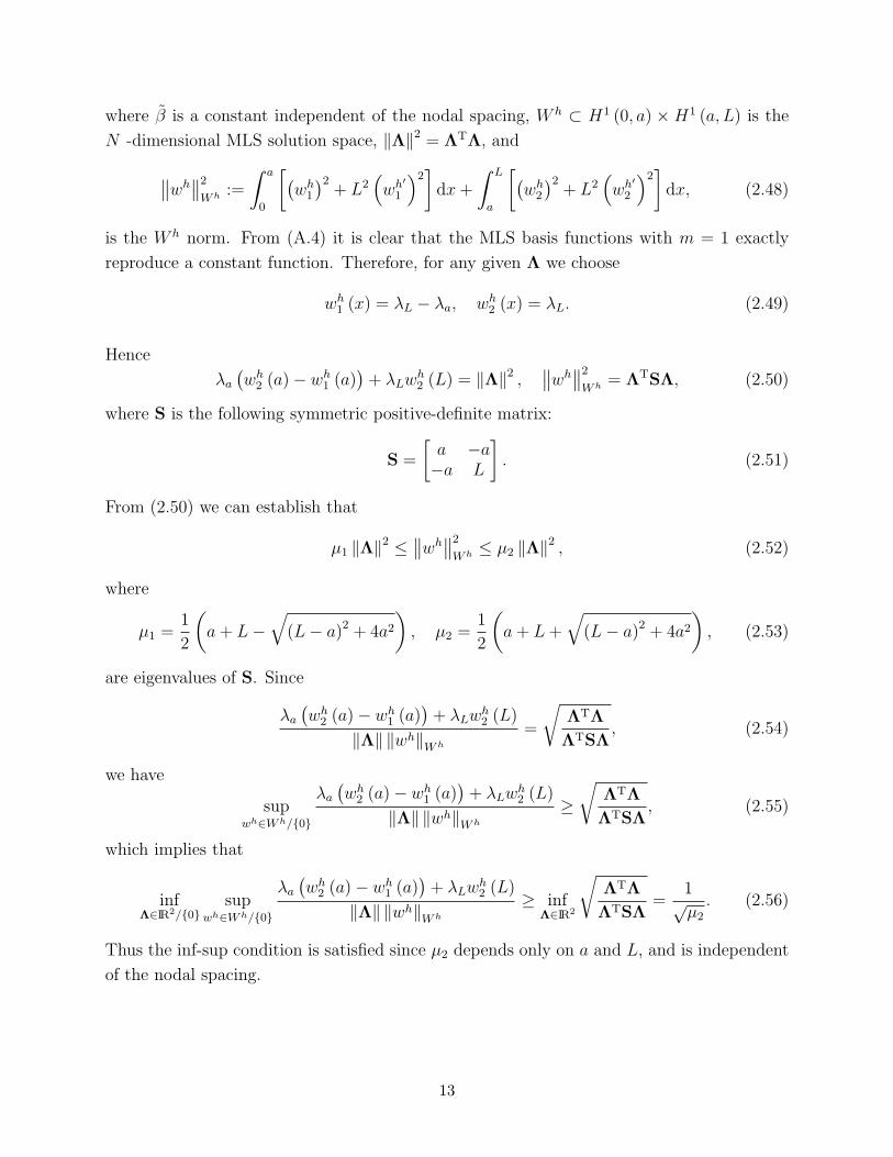
where β is a constant independent of the nodal spacing, W h ⊂ H1 (0, a) × H1 (a, L) is the
N -dimensional MLS solution space, ‖Λ‖2 = ΛTΛ, and
∥∥wh∥∥2
W h :=
∫ a
0
[(wh
1
)2+ L2
(wh′
1
)2]
dx +
∫ L
a
[(wh
2
)2+ L2
(wh′
2
)2]
dx, (2.48)
is the W h norm. From (A.4) it is clear that the MLS basis functions with m = 1 exactly
reproduce a constant function. Therefore, for any given Λ we choose
wh1 (x) = λL − λa, wh
2 (x) = λL. (2.49)
Hence
λa
(wh
2 (a)− wh1 (a)
)+ λLwh
2 (L) = ‖Λ‖2 ,∥∥wh
∥∥2
W h = ΛTSΛ, (2.50)
where S is the following symmetric positive-definite matrix:
S =
[a −a−a L
]. (2.51)
From (2.50) we can establish that
µ1 ‖Λ‖2 ≤∥∥wh
∥∥2
W h ≤ µ2 ‖Λ‖2 , (2.52)
where
µ1 =1
2
(a + L−
√(L− a)2 + 4a2
), µ2 =
1
2
(a + L +
√(L− a)2 + 4a2
), (2.53)
are eigenvalues of S. Since
λa
(wh
2 (a)− wh1 (a)
)+ λLwh
2 (L)
‖Λ‖ ‖wh‖W h
=
√ΛTΛ
ΛTSΛ, (2.54)
we have
supwh∈W h/0
λa
(wh
2 (a)− wh1 (a)
)+ λLwh
2 (L)
‖Λ‖ ‖wh‖W h
≥√
ΛTΛ
ΛTSΛ, (2.55)
which implies that
infΛ∈IR2/0
supwh∈W h/0
λa
(wh
2 (a)− wh1 (a)
)+ λLwh
2 (L)
‖Λ‖ ‖wh‖W h
≥ infΛ∈IR2
√ΛTΛ
ΛTSΛ=
1õ2
. (2.56)
Thus the inf-sup condition is satisfied since µ2 depends only on a and L, and is independent
of the nodal spacing.
13
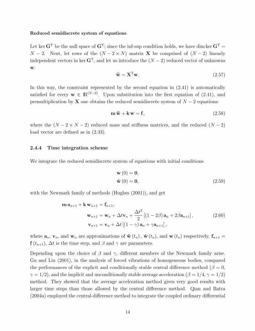
Reduced semidiscrete system of equations
Let kerGT be the null space of GT; since the inf-sup condition holds, we have dim kerGT =
N − 2. Next, let rows of the (N − 2×N) matrix X be comprised of (N − 2) linearly
independent vectors in kerGT, and let us introduce the (N − 2) reduced vector of unknowns
w:
w = XTw. (2.57)
In this way, the constraint represented by the second equation in (2.41) is automatically
satisfied for every w ∈ IR(N−2). Upon substitution into the first equation of (2.41), and
premultiplication by X one obtains the reduced semidiscrete system of N − 2 equations:
mw + kw = f , (2.58)
where the (N − 2×N − 2) reduced mass and stiffness matrices, and the reduced (N − 2)
load vector are defined as in (2.33).
2.4.4 Time integration scheme
We integrate the reduced semidiscrete system of equations with initial conditions
w (0) = 0,
w (0) = 0, (2.59)
with the Newmark family of methods (Hughes (2001)), and get
man+1 + kwn+1 = fn+1,
wn+1 = wn + ∆tvn +∆t2
2[(1− 2β) an + 2βan+1] , (2.60)
vn+1 = vn + ∆t [(1− γ) an + γan+1] ,
where an, vn, and wn are approximations of w (tn) , w (tn), and w (tn) respectively, fn+1 =
f (tn+1), ∆t is the time step, and β and γ are parameters.
Depending upon the choice of β and γ, different members of the Newmark family arise.
Gu and Liu (2001), in the analysis of forced vibrations of homogeneous bodies, compared
the performances of the explicit and conditionally stable central difference method (β = 0,
γ = 1/2), and the implicit and unconditionally stable average acceleration (β = 1/4, γ = 1/2)
method. They showed that the average acceleration method gives very good results with
larger time steps than those allowed by the central difference method. Qian and Batra
(2004a) employed the central-difference method to integrate the coupled ordinary differential
14

equations derived by the MLPG approximation of the transient thermoelastic problem for a
functionally graded material.
Here we also use these two methods, and both the consistent, and the lumped mass matrices.
For the average acceleration method we set
∆t = 10−2T, T =2
5τ,
τ :=a
c1
+L− a
c2
, (2.61)
c1 =
√E1
ρ1
, c2 =
√E2
ρ2
,
where τ is the time when the wave is reflected at the clamped end, and c1 and c2 are wave
speeds in the two materials. For values assigned to material parameters the first reflection
of the wave occurs at the clamped end.
2.4.5 Numerical evaluation of domain integrals
Since the MLS basis functions are not polynomials, it is difficult to integrate accurately the
discrete local weak forms associated with the MLPG6 formulation, and obtain the mass, and
the stiffness matrices.
We adopt the integration procedure proposed by Atluri, Cho and Kim (1999). The idea is
sketched in Figure 2.5, where a possible arrangement of nodes is shown. The integration
on ΩiS is performed by carrying out the integration on each subregion, obtained by dividing
ΩiS by boundaries of subdomains of other nodes in the neighborhood of node i. With this
method, integrals are evaluated with five quadrature points in each intersected region.
2.5 Numerical results and comparisons
2.5.1 Values of parameters
Results have been computed for following values of the material parameters
%1 = 7860kg/m3, E1 = 200GPa,
%2 = 2710kg/m3, E2 = 70GPa,(2.62)
corresponding to steel (material “1”) and aluminum (material “2”). The geometry is defined
by
L = 50mm, a = L/2 = 25mm. (2.63)
15

For these values we have
τ = 9.87µs, T = 3.95µs. (2.64)
The numerical value of P has been chosen as
P = 100MPa. (2.65)
The MLS basis functions are generated by complete monomials of degree 1. Except when we
discuss convergence of the solution with an increase in the number of uniformly spaced nodes,
results presented below have been computed with 81 uniformly spaced nodes. When we
model the discontinuity with either the jump function or the modified MLS basis functions
the domain [0, L] is discretized with equally spaced nodes with one node placed at the
interface. In both cases the semi-support ri of the weight function Wi is
ri =
2L
N − 1, i = 2, 3, ..., N − 1
4L
N − 1, i = 1, N
; (2.66)
and for the modified MLS basis functions the semi-support of the weight function for the
node at the interface is set equal to 4L/ (N − 1).
When using a Lagrange multiplier to enforce the continuity of displacements at x = a, an
equal number of uniformly spaced nodes is used in the domains [0, a] and [a, L], and (2.66)
holds in each homogeneous part of the bar with L equal to the segment length and N equal
to the total number of nodes in the segment.
From numerical experiments it has been found that the choice of the radius rJ of the jump
function support strongly affects the accuracy of computed results. Here we take
rJ =N
2
L
N − 1; (2.67)
thus one-half of nodes used in the discretization are included in the jump function semisup-
port.
2.5.2 Convergence analysis
For each of the three methods of accounting for the material discontinuity at x = a, conver-
gence tests are performed for both the solution of a static problem, and mode shapes of the
bimaterial clamped bar. Two relative error norms are used for this purpose:
• Relative L2 error norm √√√√∫ L
0(wh − we)2 dx∫ L
0(we)2 dx
; (2.68)
16

• Relative H1 error norm√√√√√∫ L
0
((wh − we)2 + L2
((wh)′ − (we)′
)2)
dx
∫ L
0
((we)2 + L2
((we)′
)2)
dx; (2.69)
where superscripts h and e refer to the MLPG6 numerical solution, and the analytical so-
lution respectively. For the static deformation with constant uniformly distributed load
P/L, Figure 2.6 shows variations of the relative L2 and H1 error norms with an increase
in the number of nodes obtained with, and without employing one of the three techniques
to account for the material discontinuity at x = a. Results have also been computed with
the FEM with piecewise linear basis functions, and a node placed at the interface. In this
and other Figures, notations J, L and MMLS signify, respectively, results obtained with the
methods of jump function, the Lagrange multipliers, and the modified MLS basis functions.
The plots reveal the monotonic convergence of the MLPG solution; the error without treat-
ment of the material discontinuity, denoted by the curve marked MLS, is higher than that
with the FEM, with convergence rates of 1 (0.5) and 2 (1), respectively, in the L2 (H1) norm.
When a special technique is used to treat the material discontinuity, the error in the MLPG
solution is always lower than that with the FEM, and the MLPG solution converges faster to
the analytical one at approximate rates of 2.5 and 1.5 respectively in the L2 and H1 norms.
The need for treating the material discontinuity is evident from examining Figure 2.7, where
the axial displacement derivative near the interface computed with and without the use of
these special methods is depicted. A treatment of discontinuity is necessary in order to
accurately model the jump in the displacement gradient at the interface x = a; however, the
displacement gradient computed away from x = a without employing any one of the three
methods is close to the analytical one. We have plotted the percentage error in the four
numerical solutions in Figure 2.7. It is evident that without using a method to account for
the discontinuity in the displacement gradient at x = a, the error in the computed solution
exceeds 50%. However, when any one of the three methods is used to consider the material
discontinuity, then the maximum error in the displacement gradient is less than 0.5%.
The numerical eigenfrequencies, and mode shapes are obtained by searching for solutions of
the type
w (t) = w exp (iωt) , (2.70)
of the reduced semidiscrete system of equations, and discarding the applied loads. Therefore,
the following eigenvalue problem arises:(k− ω2m
)w = 0. (2.71)
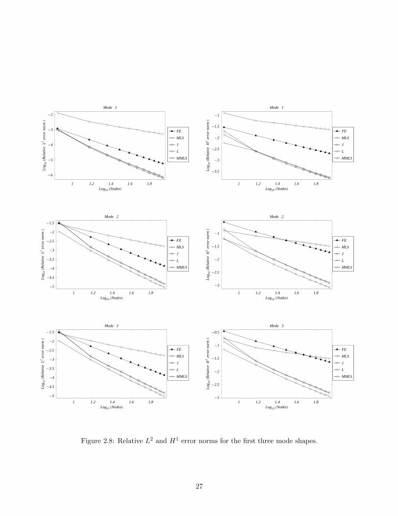
In Figure 2.8, we report the relative L2 and H1 error norms of the first three mode shapes; the
mode shapes are shown in Figure 2.9. As before, the MLPG6 solution without treatment
17

of the material discontinuity gives higher errors than the MLPG6 solutions obtained by
modeling the material discontinuity with any one of the three techniques. In both the L2 and
the H1 norms, whereas the rate of convergence of the numerical solution without treatment
of material discontinuity is lower than that of the FE solution, the MLPG6 solutions with the
material discontinuity treatment converge faster. For the first three modes, the convergence
rates in the L2 norm with and without treatment of discontinuity are 2.5 and 1.5 respectively,
against a convergence rate of 2 for the FEM. In the H1 norm, the corresponding convergence
rates are 1.5, 0.5 and 1 respectively.
In Figure 2.10 the relative errors in the first two eigenfrequencies are reported; the analyt-
ically computed first two eigenfrequencies are 0.108MHz, and 0.528MHz. In both cases,
the convergence rates are 3 and 1 for the MLPG6 solutions with, and without the treatment
of material discontinuity respectively, and 2 for the FE solution. Furthermore, frequencies
converge monotonically from above to their analytical values. For the MLPG1 formulation
of plate-theory equations, Qian, Batra and Chen (2003b) found that the first four flexural
frequencies did not converge from above with an increase in the number of nodes.
2.5.3 Forced vibrations
The MLPG solutions have been computed by using uniformly spaced 81 nodes on the global
domain.
In Figure 2.11 we report two snapshots of the traveling stress wave computed with the
average acceleration method at
t1 =a
c1
+3T
4' 7.9µs, t2 = τ + 2T ' 17.7µs, (2.72)
and in Figure 2.12 we show the axial displacement at the same instants. Times t1 and t2 are,
respectively, the instants when 3/4th of the wave has crossed the interface x = a between
the two materials, and when the two waves reflected from the free, and the clamped edges
overlap at x = a. Comparisons have been made with analytical solutions obtained by setting
j = 3 in summations (B.16), and (B.17), since for this value of j
maxt∈t1,t2
(∫ L
0
(we (x, t)|j+1 − we (x, t)|j
)2
dx
)≤ 10−15L3, (2.73)
where we (x, t)|j is the analytical solution in (B.16) and (B.17) computed for a given value
of j. The good agreement with the analytical results shows that all three methods for the
treatment of material discontinuity are able to capture well both the reflection of, and the
interaction among propagating waves; the numerical solutions virtually overlap the analytic
solution.
18

In Figure 2.13 we depict the time history of the axial displacement at the left end computed
with the central difference method by using both the consistent, and the lumped mass
matrices, with ∆t = 0.9∆tcr and 1.01∆tcr respectively. The critical time step is given by
∆tcr =2
max(ωh
i
) . (2.74)
Mass matrixConsistent Lumped
Jump function 0.0393 0.204Lagrange multiplier 0.0671 0.203
Modified MLS 0.0671 0.203
Table 2.1: Critical time step, ∆tcr [µs], for different methods of accounting for material disconti-nuity.
Here ωhi is i-th natural eigenfrequency of the system. Values of ∆tcr for the consistent, and
the lumped mass matrices, and the three methods of accounting for the material discontinuity
are listed in Table 2.1. Comparisons are made with analytical solutions obtained by summing
up to j = 7 in (B.16) and (B.17), since for this value of j
∫ t
0
(we (0, t)|j+1 − we (0, t)|j
)2
dt ≤ 10−15L2t, (2.75)
where we (x, t)|j is the analytical solution computed for a given value of j, and
t = 8 (a/c1 + (L− a)/c2) is the maximum time considered in the computations.
Whereas for the lumped mass matrix obtained by the row sum technique ∆tcr has the same
value for the three methods of accounting for the material discontinuity, it is not so for
the consistent mass matrix; ∆tcr for the method of jump function is nearly one-half of that
for the other two methods. A possible explanation is that the jump function technique
with the consistent mass matrix modifies the basis functions unfavorably for the maximum
eigenfrequency of the system. However, when the lumped mass matrix is obtained by the
row sum technique, the effect of the modification of basis functions is eliminated, and the
maximum natural frequency is the same for the three methods.
Solutions obtained with the three methods of accounting for the material discontinuity es-
sentially coincide with the analytical solution of the problem. Results plotted in Figure 2.13
signify the well known fact that the solution computed with ∆t < ∆tcr is stable, and that
with ∆t > ∆tcr is unstable. A comparison of plots of Figures 2.13a and 2.13c reveals that
the consistent mass matrix gives lower errors than the lumped mass matrix.
For the average acceleration method, only the consistent mass matrix is considered. Figure
2.13 exhibits the well known fact that the average acceleration algorithm is unconditionally
19

stable, as evidenced by the stability of the solution even when the time step size equals
1.5∆tconsistentcr , and 1.5∆tlumped
cr ∼ 0.3µs.
In Figure 2.14 we report the time history of the jump∣∣σh
(a+, t
)− σh(a−, t
)∣∣ , (2.76)
in the axial stress at the interface computed by using the method of (a) the jump function,
(b) the Lagrange multiplier, and (c) the modified MLS basis functions. Ideally it should be
zero for all times. As we can see, the method (a) is the most accurate; this is because it
models both the displacement continuity, and the axial stress continuity at x = a, while with
the other two techniques the essential boundary condition (2.13) is directly enforced but the
axial stress continuity (2.14) is weakly satisfied.
For the average acceleration method and the consistent mass matrix, Figure 2.15 exhibits
the effect of decreasing the time step size on the L2 error norm of the axial stress at times
7.91µs and 17.8µs. The MLPG method with one of the three methods of considering the
material discontinuity gives lower errors than the FEM.
Batra, Porfiri and Spinello (2004), and Qian and Batra (2004a) have compared the MLPG
and the FE formulations for transient problems.
2.6 Conclusions
We have used the meshless local Bubnov-Galerkin (MLPG6) method to study free, and
forced vibrations of a segmented bar comprised of two materials. Because of the higher-
order differentiability of the MLS basis functions, special techniques are needed to accurately
model jumps in displacement gradients at the material interfaces. Here, we have employed
methods of (a) the jump function, (b) the Lagrange multiplier, and (c) the modified MLS
basis functions with discontinuous derivative. In all cases the essential boundary condition
has been enforced by introducing a Lagrange multiplier.
The stability of methods has been assessed by analytically proving the inf-sup condition.
Reduced semidiscrete systems are derived, where constraints are automatically satisfied.
The direct analysis of forced vibrations is performed by using the β-Newmark family of
methods, and the spatial integration in the MLPG formulation uses Gauss quadrature rules.
Both the lumped, and the consistent mass matrices with the central-difference method are
used, while only consistent mass matrix with the average acceleration method is considered.
Numerical results for a bimaterial bar, clamped at one end, and free at the other end,
computed with the MLPG6 formulations have been compared with those obtained with the
FEM, and analytically. Both for static, and dynamic problems studied, convergence rates
20

of the MLPG6 solution without any treatment of material discontinuities are lower than
those of the FE solution. However, when any one of the three techniques to account for the
material discontinuity is used, the MLPG6 solution converges faster than the FE solution.
For a fixed number of nodes, errors in the MLPG6 solution are lower than those in the FE
solution. This is a very favorable feature of the MLPG6 method with respect to the FEM;
the higher computational time required to evaluate domain integrals is balanced somewhat
by a gain in accuracy.
The analysis of the transient response due to an axial traction of finite time duration applied
at one end of the bar reveals a very good agreement between the MLPG6 and the analytical
solutions. Each technique for the treatment of the material discontinuity is able to capture
the wave reflection, and interaction between waves at the interface between two materials.
Whereas the method of the special jump function is the most accurate in modeling the
continuity of the axial stress at the interface because of the introduction of a dedicated
degree of freedom, the size of the support of the jump function significantly affects the
accuracy of computed results. Numerical experiments suggest that, for this problem, about
one half of the nodes employed in the discretization of the global domain need to be included
in the radius of the support of the jump function in order to ensure good results. For the
consistent mass matrix, the critical time step size for the method of jump function is nearly
one-half of that for the other two methods. Both the method of Lagrange multipliers, and the
MLS discontinuous basis functions can be generalized to more complex geometries involving
material discontinuities.
For the lumped mass matrix, the three methods of accounting for the material discontinuity
give the same maximum frequency of the segmented bar. However, when the consistent mass
matrix is employed, the maximum natural frequency computed with the method of jump
function is nearly twice of that for the other two methods. The largest frequency computed
with the lumped mass matrix is nearly one-third of that obtained with the consistent mass
matrix. Thus for the explicit time-integration method, it is more efficient to use the lumped
mass matrix.
21

0 a = L2 L
1 2 3 4 5 6 7 8 9 10 11
2r6
0 a = L2 L
1 2 3 4 5 6 7 8 9 10 11
2r6
0 a = L2 L
1 2 3 4 5 6 7 8 9 10 11
2r6
0 a = L2 L
1 2 3 4 5 6 7 8 9 10 11
2r6
0 a = L2 L
1 2 3 4 5 6 7 8 9 10 11
2r6
0 a = L2 L
1 2 3 4 5 6 7 8 9 10 11
2r6
Figure 2.1: Modified MLS basis functions for nodes 1 through 6 obtained with m = 2 and ri =3L/ (N − 1).
22

a
L
p
x
Figure 2.2: Schematic sketch of the problem studied.
0 Tt
P
p
Figure 2.3: Plot of the time-dependent axial traction applied at x = 0.
23

-1 1
x- a
rJ
0.17
Jump function
-1 1
x- a
rJ
-0.5
0.5
Jump function derivative
Figure 2.4: Plots of the jump function κ(
x−arJ
), and its derivative.
ix
S
iΩ
Sub-regions for integration
1ix −2i
x − 1ix + 2i
x +
S
1i +ΩS
2i +ΩS
1i −ΩS
2i −Ω
Figure 2.5: Subdomain ΩiS of node xi, and integration subregions obtained by the intersection of
ΩiS with supports of domains of influence of neighboring nodes.
24

1 1.2 1.4 1.6 1.8Log10 HNodesL
-5
-4
-3
-2
Log
10HR
elat
ive
L2
erro
rno
rmL
Static solution
MMLS
L
J
MLS
FE
(a)
1 1.2 1.4 1.6 1.8Log10 HNodesL
-3.5
-3
-2.5
-2
-1.5
-1
Log
10HR
elat
ive
H1
erro
rno
rmL
Static solution
MMLS
L
J
MLS
FE
(b)
Figure 2.6: (a) Relative L2 error norm and, (b) relative H1 error norm for static deformationsunder uniformly distributed load along the length of the bar.
25

23 24 25 26 27 28x
-0.0007
-0.0006
-0.0005
-0.0004
-0.0003
-0.0002
Axial displacement derivative
MMLS
L
J
MLS
Exact
(a)
24 25 26 27x
10
20
30
40
50
Percentage error, MLS
(b)
23 24 25 26 27 28x
0.1
0.2
0.3
0.4
0.5Percentage error
MMLS
L
J
(c)
Figure 2.7: (a) Axial displacement gradient near the material interface for a static deformation,and the percentage error in the derivative of the solution for the uniformly distributed load, P/L,obtained with (b) the MLS basis functions without treatment of the material discontinuity; (c) theMLS basis functions with the three methods of treating the material discontinuity.
26
1 1.2 1.4 1.6 1.8Log10 HNodesL
-6
-5
-4
-3
-2
Log
10HR
elat
ive
L2
erro
rno
rmL
Mode 1
MMLS
L
J
MLS
FE
1 1.2 1.4 1.6 1.8Log10 HNodesL
-3.5
-3
-2.5
-2
-1.5
-1
Log
10HR
elat
ive
H1
erro
rno
rmL
Mode 1
MMLS
L
J
MLS
FE
1 1.2 1.4 1.6 1.8Log10 HNodesL
-5
-4.5
-4
-3.5
-3
-2.5
-2
-1.5
Log
10HR
elat
ive
L2
erro
rno
rmL
Mode 2
MMLS
L
J
MLS
FE
1 1.2 1.4 1.6 1.8Log10 HNodesL
-3
-2.5
-2
-1.5
-1
Log
10HR
elat
ive
H1
erro
rno
rmL
Mode 2
MMLS
L
J
MLS
FE
1 1.2 1.4 1.6 1.8Log10 HNodesL
-5
-4.5
-4
-3.5
-3
-2.5
-2
-1.5
Log
10HR
elat
ive
L2
erro
rno
rmL
Mode 3
MMLS
L
J
MLS
FE
1 1.2 1.4 1.6 1.8Log10 HNodesL
-3
-2.5
-2
-1.5
-1
-0.5
Log
10HR
elat
ive
H1
erro
rno
rmL
Mode 3
MMLS
L
J
MLS
FE
Figure 2.8: Relative L2 and H1 error norms for the first three mode shapes.
27

10 20 30 40 50x
0.025
0.05
0.075
0.1
0.125
0.15
0.175
Mode 1
MMLS
L
J
Exact
10 20 30 40 50x
-0.2
-0.15
-0.1
-0.05
0.05
0.1
Mode 2
MMLS
L
J
Exact
10 20 30 40 50x
-0.1
0.1
0.2
Mode 3
MMLS
L
J
Exact
Figure 2.9: First three mode shapes of the segmented bar.
28

1 1.2 1.4 1.6 1.8Log10 HNodesL
-7
-6
-5
-4
-3
-2
Log
10HR
elat
ive
erro
rfr
eque
ncyL
Frequency 1
MMLS
L
J
MLS
FE
1 1.2 1.4 1.6 1.8Log10 HNodesL
-6
-5
-4
-3
-2
Log
10HR
elat
ive
erro
rfr
eque
ncyL
Frequency 2
MMLS
L
J
MLS
FE
Figure 2.10: Relative error in the estimation of the first two natural frequencies.
29

0 10 20 30 40 50x HmmL
-0.04
-0.02
0
0.02
0.04
Axi
alSt
ressHG
PaL
t = 7.90 Μs
MMLS
L
J
Exact
(a)
0 10 20 30 40 50x HmmL
0
0.01
0.02
0.03
0.04
0.05
0.06
0.07
Axi
alSt
ressHG
PaL
t = 17.7 Μs
MMLS
L
J
Exact
(b)
Figure 2.11: Snapshots of the traveling stress wave at (a) t = ac1
+ 3T4 , and (b) t = τ + 2T .
30

0 10 20 30 40 50x HmmL
-0.008
-0.006
-0.004
-0.002
0
Axi
alD
ispl
acem
entHm
mL
t = 7.90 Μs
MMLS
L
J
Exact
(a)
0 10 20 30 40 50x HmmL
-0.012
-0.01
-0.008
-0.006
-0.004
-0.002
0
Axi
alD
ispl
acem
entHm
mL
t = 17.7 Μs
MMLS
L
J
Exact
(b)
Figure 2.12: Snapshots of the displacement wave at (a) t = ac1
+ 3T4 , and (b) t = τ + 2T .
31
0 20 40 60 80t HΜsL
-0.01
-0.005
0
0.005
0.01
wH0
,tL
Central difference, consistent mass matrix, Dt=0.9 Dtcr
MMLS
L
J
Exact
0.5 1 1.5 2 2.5 3 3.5t HΜsL
-0.04
-0.02
0
0.02
0.04
wH0
,tL
Central difference, consistent mass matrix, Dt=1.01 Dtcr
MMLS
L
J
Exact
(a) (b)
0 20 40 60 80t HΜsL
-0.01
-0.005
0
0.005
0.01
wH0
,tL
Central difference, lumped mass matrix, Dt=0.9 Dtcr
MMLS
L
J
Exact
1 2 3 4 5 6t HΜsL
-0.04
-0.02
0
0.02
0.04
wH0
,tL
Central difference, lumped mass matrix, Dt=1.01 Dtcr
MMLS
L
J
Exact
(c) (d)
0 20 40 60 80t HΜsL
-0.01
-0.005
0
0.005
0.01
wH0
,tL
Average acceleration, Dt=1.5 Dtcrconsistent
MMLS
L
J
Exact
0 20 40 60 80t HΜsL
-0.01
-0.005
0
0.005
0.01
wH0
,tL
Average acceleration, Dt=1.5 Dtcrlumped
MMLS
L
J
Exact
(e) (f)
Figure 2.13: Time history of the free end displacement obtained with (a) central difference,consistent mass matrix, and ∆t = 0.9∆tcr; (b) central difference, consistent mass matrix, and∆t = 1.01∆tcr; (c) central difference, lumped mass matrix, and ∆t = 0.9∆tcr; (d) central differ-ence, lumped mass matrix, and ∆t = 1.01∆tcr; (e) average acceleration, consistent mass matrix,and ∆t = 1.5∆tconsistent
cr ; (f) average acceleration, consistent mass matrix, and ∆t = 1.5∆tlumpedcr .
32

0 20 40 60 80t HΜsL
0
0.00005
0.0001
0.00015
0.0002
0.00025
0.0003
0.00035
Stre
ssju
mp
atth
ein
terf
ace
Jump function
(a)
0 20 40 60 80t HΜsL
0
0.001
0.002
0.003
0.004
0.005
Stre
ssju
mp
atth
ein
terf
ace
Lagrange multiplier
(b)
0 20 40 60 80t HΜsL
0
0.001
0.002
0.003
0.004
0.005
Stre
ssju
mp
atth
ein
terf
ace
Discontinuous basis function
(c)
Figure 2.14: Time history of the jump in the axial stress at the interface using (a) the special jumpfunction, (b) the Lagrange multiplier, and (c) the modified MLS basis functions with discontinuousderivatives.
33

1.4 1.6 1.8 2 2.2 2.4 2.6Log10HTDtL
-4
-3.5
-3
-2.5
Log
10HR
elat
ive
L2
erro
rno
rmL
t = 7.91 Μs
MMLS
L
J
MLS
FE
1.4 1.6 1.8 2 2.2 2.4 2.6Log10HTDtL
-4
-3.5
-3
-2.5
Log
10HR
elat
ive
L2
erro
rno
rmL
t = 17.8 Μs
MMLS
L
J
MLS
FE
Figure 2.15: At two different times, effect of the time step size on the L2 relative error norm in theaxial displacement.
34
Chapter 3
Pull-in Instability in ElectricallyActuated Narrow Microbeams
3.1 Introduction
The recent technological developments have opened promising research opportunities and
engineering priorities in micromechanics. The study of electrostatically actuated MicroElec-
troMechanical Systems (MEMS) is a branch of micromechanics. These MEMS find wide
applications in switches (see, e.g., Nguyen, Katehi and Rebeiz (1998)), micro-mirrors (see,
e.g., Hung and Senturia (1999)) and micro-resonators (see, e.g., Tilmans and Legtenberg
(1994)). At the microscopic scale high energy densities and large forces are available, and
the electrostatic actuation may be more effective than other kinds of actuation.
An electrostatically actuated microbeam is an elastic beam suspended above a stationary
rigid plate, both made of conductive materials, and a dielectric medium filling the gap be-
tween them. An applied electric voltage between the two electrodes results in the deflection
of the elastic beam and a consequent change in the MEMS capacitance. The applied electro-
static force has an upper limit beyond which the electrostatic Coulomb force is not balanced
by the elastic restoring force in the deformable beam, the beam spontaneously deflects to-
wards the stationary rigid plate, and the device collapses. This phenomenon, called pull-in
instability, was simultaneously observed experimentally by Taylor (1968) and Nathanson,
Newell, Wickstrom and Davis (1977). The accurate estimation of the pull-in voltage is cru-
cial in the design of electrostatically actuated MEM devices. In particular, in micro-mirrors
(see, e.g., Hung and Senturia (1999)) and micro-resonators (see, e.g., Tilmans and Legtenberg
(1994)) the designer avoids this instability in order to achieve stable motions; in switching
applications (see, e.g., Nguyen, Katehi and Rebeiz (1998)) the designer exploits this effect
Material in this Chapter is part of the paper “Electromechanical Model of Electrically Actuated Narrow Mi-crobeams,” accepted for publication in Journal of Microelectromechanical Systems
35

to optimize the device’s performance.
Accurate estimates of the pull-in parameters have been obtained by three-dimensional (3-D)
numerical simulations based on either the finite element (FE) or the boundary element anal-
yses (see, e.g., Gabbay, Mehner and Senturia (2000) and Senturia, Harris, Johnson, Kim,
Nabors, Shulman and White (1992)); however, these approaches are time-consuming. There-
fore, considerable effort has been devoted to developing reliable 1-D distributed models of
electrostatically actuated microbeams. In Tilmans and Legtenberg (1994), a wide clamped-
clamped microbeam is modelled with the classical linear beam theory, and the electrostatic
force is computed by completely discarding fringing field effects. These assumptions are
justified for small beam deflections and wide beams. In Osterberg and Senturia (1997), an
effective Young’s modulus is considered in order to account for plane stress and plane strain
deformations appropriate for narrow and wide beams respectively. The effects of fringing
field is considered by accounting for the microbeam’s finite width but neglecting its finite
thickness. In Abdel-Rahman, Younis and Nayfeh (2002), the beam mid-plane stretching is
accounted for in order to treat large deflections. Nevertheless, no improvements with respect
to Tilmans and Legtenberg (1994) on the electric modeling are considered, rendering this
model suitable for a wide microbeam with initial gap size comparable with the beam thick-
ness. In Kuang and Chen (2004), the fringing field correction of Osterberg and Senturia
(1997) is combined with the finite deflection approach of Abdel-Rahman, Younis and Nayfeh
(2002) resulting in a model that accurately predicts the pull-in parameters of wide beams
undergoing moderate displacements. None of these works is applicable to narrow beams
where effects of fringing fields due to the finite thickness are not negligible, as observed in
Pamidighantam, Puers, Baert and Tilmans (2002).
Furthermore, the consideration of the mid-plane stretching makes the governing equation
nonlinear, and the problem of numerically extracting the pull-in parameters more chal-
lenging. The shooting method used in Abdel-Rahman, Younis and Nayfeh (2002) to solve
nonlinear differential equations relies on good initial estimates of unknown parameters and
may diverge. In Younis, Abdel-Rahman and Nayfeh (2003) two variants of the Galerkin
method are employed by using the beam mode shapes as basis functions. In the first vari-
ant the electrostatic force is expanded in Taylor series around the undeformed configuration
and terms up to the fifth order are retained. The second variant accounts exactly for the
electrostatic force. The estimate of the pull-in parameter computed with the first method
does not agree well with that obtained with the shooting method. The pull-in parameter
obtained from the second variant is very sensitive to the number of modes used as basis,
and acceptable results are obtained only when an odd number of modes greater than one
are included in the basis functions. Both techniques neglect fringing field effects. The use
of mode shapes as basis limits the applicability of the method to beam geometries for which
36

eigenvalues and eigenfunctions can be easily computed. In Kuang and Chen (2004), the dif-
ferential quadrature method is used and computed results seem very accurate; nevertheless,
the global nature of the method seems to forbid its application to more complicated MEMS
geometries.
In this Chapter, we present a model for analyzing narrow microbeams undergoing finite
deflections. The beam is modelled by using a large deflection theory, see, e.g., Landau
and Lifshitz (1986). This model does not account for finite deformations, and is applicable
when the MEMS gap size and the microbeam thickness are considerably smaller than the
beam span. Indeed, small strains are experienced whenever the microbeam deflection is
much smaller than the microbeam length, even if the maximum deflection exceeds the beam
thickness. We solve the resulting nonlinear fourth-order differential equation by using two
distinct approaches: (i) reducing the distributed system to a one-degree-of-freedom system,
and (ii) retaining the distributed system, and using the MLPG and the FE methods in
conjunction with the efficient Displacement Iteration Pull-In Extraction (DIPIE) algorithm
developed in Degani-Bochobza, Elata and Nemirovsky (2002). In particular, we derive a
consistent electromechanical model where finite thickness of the beam is considered in both
the mechanical and the electrical models. With the Method of Moments (MoM), see, e.g.,
Harrington (1993), an expression for the electrostatic load is established which simultane-
ously accounts for the fringing field capacitance due to finite width and finite thickness of
the microbeam. The approach followed here is similar to that used in structural mechanics
to study Saint-Venant problems, see, e.g., Iesan (1987). That is, deformations of a slender
beam are studied by initially solving a 2-D problem defined on the cross-section of the beam
and using these results to build a 1-D model of the beam with distributed forces/loads act-
ing on its length. Whereas in Gabbay, Mehner and Senturia (2000) a reduced order discrete
model valid for a specific MEMS is deduced from 3-D numerical simulations, here a 1-D dis-
tributed model of a narrow microbeam is proposed with 2-D numerical simulations needed
to determine an expression for the electrostatic force. The distributed 1-D model is studied
using both the MLPG and the FE methods. Basis functions for representing the test and
the trial functions in the MLPG method are constructed using the GMLS approximation.
While in the FE work Hermitian basis functions (i.e., beam elements) are exploited. The
present reduced order one-degree-of-freedom model differs from the classical mass-spring
model of Nathanson, Newell, Wickstrom and Davis (1977) since we account for the axial
stress, nonlinear stiffening, charge redistribution, and fringing fields. It also differs from that
of Younis, Abdel-Rahman and Nayfeh (2003) since we retain the complete nonlinear behavior
of the electrostatic force and consider fringing fields, and it differs from that of Pamidighan-
tam, Puers, Baert and Tilmans (2002) since we simultaneously treat the pull-in voltage
and deflections as unknowns, i.e. the pull-in deflection is not empirically chosen as was
done in Pamidighantam, Puers, Baert and Tilmans (2002). Two sample problems, namely
37

a cantilever and a clamped-clamped microbeam are considered. Results from the proposed
one-degree-of-freedom and the distributed models are compared with those available in the
literature, i.e. Osterberg and Senturia (1997), Abdel-Rahman, Younis and Nayfeh (2002),
Kuang and Chen (2004) , and also with those obtained from 3-D FE simulations. Some of the
3-D FE results for a cantilever beam are borrowed from Pamidighantam, Puers, Baert and
Tilmans (2002). Other results for the cantilever beam, and results for the clamped-clamped
microbeam have been obtained by using the commercial FE code ANSYS.
Three goals of the present work are: (i) propose a consistent 1-D distributed electrome-
chanical model for a narrow microbeam, (ii) establish a reduced order one-degree-of-freedom
model that gives a good estimate of the pull-in parameters (deflection and voltage), and
(iii) extend the MLPG method employed earlier to analyze linear beam problems to the
analysis of those nonlinear beam problems where nonlinearities arise simultaneously due to
electrostatic loads and membrane stretching.
The rest of the Chapter is organized as follows. In Section 3.2, we give governing equations
of an electrostatically actuated clamped-clamped and a cantilever narrow microbeam; in
Section 3.3, we derive an expression for the distributed electrostatic force that simulates
well the fringing field effects. In Section 3.4, we describe a one-degree-of-freedom model,
and in Section 3.5, we briefly present the MLPG and the FE methods and apply the DIPIE
algorithm for extracting the pull-in parameters. In Section 3.6, we compare the proposed
fringing fields corrections with some of the classical formulas available in the literature. The
proposed one-degree-of-freedom, and the distributed electromechanical models are validated
by comparing predictions from them with those from other distributed models, and from
ANSYS and COVENTORWARE FE solutions. Section 3.7 summarizes conclusions of this
work. The Method of Moments used in Section 3.3 is briefly outlined in Appendix C. The
fundamentals of the GMLS approximation are recalled in Appendix A.2.
3.2 Model development
We consider a narrow microbeam of length `, width b, and thickness h either clamped-
clamped or clamped-free, as depicted in Figures 3.1 and 3.2. The microbeam is suspended
above an infinite ground plane with an initial gap g0. Both bodies are perfect conductors
and are separated by a dielectric medium of permittivity ε0εr, where ε0 is the vacuum per-
mittivity, and εr is the relative permittivity. A positive potential difference V between the
two conductors causes the microbeam to electrostatically deflect downwards.
38

3.2.1 Governing equation for mechanical deformations
Within the large deflection beam theory, see, e.g., Abdel-Rahman, Younis and Nayfeh (2002),
the deflection w in the z direction is given by, (see Figures 3.3 and 3.4)
EId4w
dx4−N (w)
d2w
dx2= Fe (w) , (3.1)
where E is Young’s modulus, I the moment of inertia of the cross section about the y
axis, N the axial force which is constant along the beam axis, Fe the deflection dependent
electrostatic force per unit length, and x the axial coordinate. A beam is considered narrow,
when its width b is less than five times its thickness h, see, e.g., Osterberg and Senturia (1997).
For wide beams the mechanical stiffness, EI, should be modified as given in Osterberg and
Senturia (1997).
For a cantilever beam the axial force vanishes, while for a clamped-clamped beam it is given
by
N (w) =EA
2`
∫ `
0
(dw
dx
)2
dx + N0, (3.2)
where A is the area of cross section of the beam, and N0 is the residual axial load. For a
narrow beam, the residual axial load is N0 = σA, where σ is the effective residual axial stress.
The residual stress is equal to σ0 (1− ν) , where σ0 is the initial uniform biaxial stress in the
material, see, e.g., Osterberg and Senturia (1997) and ν is Poisson’s ratio for the material of
the beam.
For a fixed-fixed beam, the deflection is subjected to the following four kinematic boundary
conditions:
w (0) = 0,dw
dx(0) = 0, w (`) = 0,
dw
dx(`) = 0, (3.3)
while for a cantilever beam the deflection should satisfy the two kinematic boundary condi-
tions at the clamped end, and the two kinetic boundary conditions at the free end x = `:
w (0) = 0,dw
dx(0) = 0,
d2w
dx2(`) = 0,
d3w
dx3(`) = 0. (3.4)
3.2.2 Distributed force due to electric field
The distributed force, Fe(w), on the deformable microbeam due to the electric field depends
on the potential difference between the two conductors and on their geometries. Since only
small deformations of the beam are considered, it is reasonable to assume that at every point
x the electrostatic force per unit length, Fe, depends only on the local deflection w (x) and
equals the force per unit length acting on an infinitely long straight beam separated by a
distance g (x) = g0−w (x) from a ground plane as shown in Figure 3.5. The force Fe may be
39
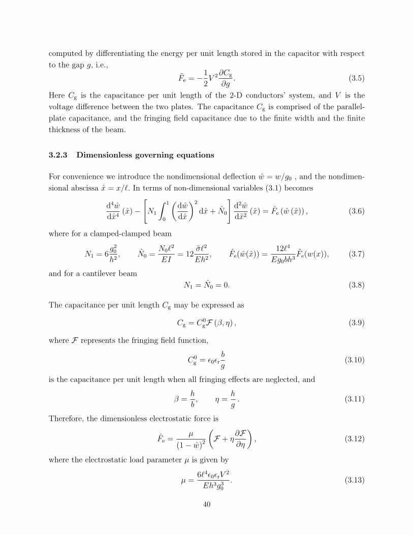
computed by differentiating the energy per unit length stored in the capacitor with respect
to the gap g, i.e.,
Fe = −1
2V 2∂Cg
∂g. (3.5)
Here Cg is the capacitance per unit length of the 2-D conductors’ system, and V is the
voltage difference between the two plates. The capacitance Cg is comprised of the parallel-
plate capacitance, and the fringing field capacitance due to the finite width and the finite
thickness of the beam.
3.2.3 Dimensionless governing equations
For convenience we introduce the nondimensional deflection w = w/g0 , and the nondimen-
sional abscissa x = x/`. In terms of non-dimensional variables (3.1) becomes
d4w
dx4(x)−
[N1
∫ 1
0
(dw
dx
)2
dx + N0
]d2w
dx2(x) = Fe (w (x)) , (3.6)
where for a clamped-clamped beam
N1 = 6g20
h2, N0 =
N0`2
EI= 12
σ`2
Eh2, Fe(w(x)) =
12`4
Eg0bh3Fe(w(x)), (3.7)
and for a cantilever beam
N1 = N0 = 0. (3.8)
The capacitance per unit length Cg may be expressed as
Cg = C0gF (β, η) , (3.9)
where F represents the fringing field function,
C0g = ε0εr
b
g(3.10)
is the capacitance per unit length when all fringing effects are neglected, and
β =h
b, η =
h
g. (3.11)
Therefore, the dimensionless electrostatic force is
Fe =µ
(1− w)2
(F + η
∂F∂η
), (3.12)
where the electrostatic load parameter µ is given by
µ =6`4ε0εrV
2
Eh3g30
. (3.13)
40

In Section 3.3 we will derive an expression for Fe applicable to a narrow microbeam.
Henceforth we drop the superimposed hat on dimensionless variables and use a prime to in-
dicate derivative with respect to the dimensionless axial coordinate. Therefore the governing
equation (3.1) in terms of nondimensional variables is
wIV (x)−N (w) w′′ (x) = Fe (w (x)) , (3.14)
where for a clamped-clamped beam
N (w) = N1
∫ 1
0
(w′)2dx + N0, (3.15)
and for a cantilever beam
N (w) = 0. (3.16)
3.2.4 Weak formulation
For a clamped-clamped microbeam, we introduce the following weak formulation, see, e.g.,
Mura and Koya (1992), of the problem described by the governing equation (3.14) and the
nondimensional version of the boundary conditions (3.3):
0 =
∫ 1
0
w′′w′′ dx + N (w)
∫ 1
0
w′w′dx−∫ 1
0
Fewdx (3.17)
+ (λ1w (0) + λ2w′ (0) + λ3w (1) + λ4w
′ (1)) +(λ1w (0) + λ2w
′ (0) + λ3w (1) + λ4w′ (1)
).
Here, λ1, λ2, λ3 and λ4 are Lagrange multipliers used to impose the four kinematic boundary
conditions ( 3.3), w is a smooth test function which need not satisfy the kinematic boundary
conditions, and λ1, λ2, λ3 and λ4 are arbitrary scalar numbers.
For a cantilever microbeam (3.17) becomes
∫ 1
0
w′′w′′ dx−∫ 1
0
Fewdx + (λ1w (0) + λ2w′ (0)) +
(λ1w (0) + λ2w
′ (0))
= 0, (3.18)
where only two Lagrange multipliers are employed since only two kinematic boundary con-
ditions are prescribed.
The consideration of Lagrange multipliers allows for the simultaneous application of the
MLPG and the FE methods. Indeed, the GMLS basis functions (see Appendix A.2) used
in the MLPG method do not have the Kronecker delta property, see, e.g., Atluri and Zhu
(1998), and special techniques, such as Lagrange multipliers, are needed to enforce kinematic
boundary conditions.
41

3.3 Computation of the electric force field
The problem of computing the capacitance per unit length of the present system of con-
ductors has been addressed in the literature on semiconductor-integrated circuits, see, e.g.,
Barke (1988), and microwave striplines, see, e.g., Collins (1992). Several empirical and ana-
lytical expressions have been proposed but none of them seem to be applicable to a narrow
microbeam.
We derive here an empirical formula for the capacitance per unit length of the line to ground
system, shown in Figure 3, for a narrow microbeam. The empirical formula is based on a
least square fitting of numerical values obtained by using the well-known Method of Moments
(MoM), see, e.g., Harrington (1993), outlined in Section 3.3 for piecewise constant basis
functions and the collocation method.
3.3.1 Empirical formula for the capacitance
The capacitance Cg of the line to ground system of Figure 3.5 equals twice the capacitance
Cg of two identical rectangular conductors depicted in Figure 3.6. Therefore, we consider
this auxiliary system involving finite size conductors and exploit symmetry conditions.
By using the MoM, we numerically compute the capacitance per unit length Cg for different
values of dimensionless parameters β and η defined in (3.11) ranging from 0.2 to 2, and 0.4 to
5 respectively. The resulting data are then least-squares fitted by a function of the following
form:
Cg = ε0εr
(η
β+ c0 + c1
(η
β
)c2
+ c3ηc4
), (3.19)
where c0, c1, c2, c3 and c4 are constants. The first term on the right hand side of (3.19)
describes the parallel-plate capacitance, the third term accounts for the fringing field capac-
itance due to the finite width b, and the fourth term models the fringing field capacitance
due to the finite thickness. Numerical values of the optimized constants are
c0 = −0.36, c1 = 0.85, c2 = 0.24, c3 = 2.5, c4 = 0.24. (3.20)
In the chosen range of variation for β and η, the maximum deviation in the capacitance
between the estimate obtained by substituting from (3.20) into (3.19) and the fully converged
numerical solution achieved by using the MoM is less than 2%. Therefore, the fringing field
that we propose to use in (3.9) is
F (β, η) = 1− 0.36β
η+ 0.85
(β
η
)0.76
+ 2.5β
η0.76. (3.21)
42

3.3.2 Validation of the capacitance estimate
In Table 3.1 we compare capacitance values computed from (3.9) by substituting the expres-
sion for the fringing field F (β, η) from relation (3.21), and from relations available in the
literature, i.e. Palmer’s formula (see, e.g., Palmer (1927))
F (β, η) = 1 +2
π
β
η
(1 + ln
(π
η
β
)), (3.22)
the parallel-plate approximation F (β, η) = 1, and the Meijs-Fokkema relation (Meijs and
Fokkema (1984))
F (β, η) = 1 + 0.77β
η+ 1.06
(β
η
)0.75
+ 1.06β
η0.5. (3.23)
We use a fully converged solution obtained with the MoM for comparing accuracies of dif-
ferent formulas. It is clear that, for narrow microbeams with 0.5 ≤ b/h ≤ 5, 0.2 ≤ g/h ≤ 2,
the Palmer formula and the parallel plate approximation give erroneous values of the capac-
itance per unit line. As stated in Meijs and Fokkema (1984), values from the Meijs-Fokkema
formula have a maximum deviation of 2% for η/β = b/g ≥ 1, 0.1 ≤ η = h/g ≤ 4, and of 6%
for η/β ≥ 0.3 and η < 10. The estimate is worst when the gap size is larger than the beam
width, i.e. g/b > 1. In this case, the error in the capacitance values from the Meijs-Fokkema
formula is ∼ 6% which is usually unacceptable. It is also evident that the proposed empirical
formula provides accurate estimates for values of β and η that are outside the range of their
values used for least squares fitting.
In Figure 3.7 we have plotted the percentage error in the capacitance versus the gap/thickness
for β = h/b = 0.2 (narrow beam), and β = 2 (significantly narrow beam) computed with
the different formulas, and taking as reference the converged numerical values obtained by
applying the MoM. As expected the present interpolation formula (3.21) provides accurate
results for both values of β. The Mejis-Fokkema relation (3.23) gives precise results for a
narrow beam but has moderate discrepancies for a significantly narrow beam. The Palmer
expression (3.22) and the parallel plate approximation which totally neglect finite thickness
of the beam provide poor estimates of the electric capacitance for narrow and significantly
narrow micro-beams yielding large errors. The electrostatic force estimated from the two
methods is acceptable only for small gaps. Since the gap varies as the beam deforms, formulas
(3.22) and (3.23) may not give accurate values of the pull-in voltage.
3.4 One-degree-of-freedom model
A closed-form solution of the boundary-value problem defined by (3.14) and the pertinent
boundary conditions cannot be found. Here we give an approximate solution based on a
43

Geometry MoM % Deviationsβ η Cg/ (ε0εr) (3.21) Meijs-Fokkema (3.23) Palmer (3.22) Parallel-Plate0.1 0.5 8.14 −1.6 −0.4 −9.2 −38.60.1 1 13.71 −0.7 < 0.1 −6.5 −27.10.1 2.5 29.61 < 0.1 0.7 −4.1 −15.70.1 5 55.38 0.2 1.0 −3.0 −9.90.1 10 106.19 0.3 1.2 2.2 −6.20.2 0.5 5.37 −1.1 −0.4 −17.2 −53.50.2 1 8.42 −0.4 −0.1 −12.3 −40.70.2 2.5 16.80 < 0.1 0.8 −8.0 −25.60.2 5 30.06 0.3 1.5 −5.6 −16.90.2 10 55.86 0.5 1.9 −4.0 −10.90.5 0.5 3.61 < 0.1 −0.8 −34.5 −72.30.5 1 5.12 0.4 −0.6 −25.7 −61.00.5 2.5 8.97 0.4 −0.7 −17.7 −44.30.5 5 14.71 0.6 2.1 −12.9 −32.10.5 10 25.50 0.9 3.4 −9.1 −21.91 0.5 2.96 0.6 −1.7 −51.9 −83.11 1 3.96 0.7 −1.8 −40.3 −74.81 2.5 6.29 0.4 −0.1 −29.3 −60.21 5 9.52 0.5 2.2 −22.4 −47.51 10 15.30 1.1 4.6 −16.4 −34.92 0.5 2.59 0.8 −2.9 −71.8 −90.42 1 3.34 0.7 −3.5 −57.3 −85.02 2.5 4.90 < 0.1 −1.7 −43.8 −74.52 5 6.88 < 0.1 1.4 −53.3 −63.72 10 10.16 0.7 5.4 −27.4 −50.95 0.5 2.34 0.3 −5.2 ∞ −95.75 1 2.92 −0.1 −6.2 −81.5 −93.25 2.5 4.03 −1.4 −4.8 −64.7 −87.65 5 5.25 −1.6 −1.0 −55.0 −81.05 10 7.04 −0.7 4.9 −45.9 −71.6
Table 3.1: Comparison between the capacitances per unit length computed by the Method ofMoments (MoM) with those from (3.9) by substituting in it the expression (3.21) for the fringingfield, and from three formulas available in the literature.
44

one-degree-of-freedom model of the MEMS. The approximate solution is constructed by ex-
pressing the dimensionless deflection field as the product of an unknown deflection parameter
ζ and a given trial function w(x) satisfying the kinematic boundary conditions:
w(x) = ζw(x). (3.24)
The governing equation for ζ is derived by multiplying both sides of (3.14) by w, integrating
over the beam span, and substituting into the resulting equation the approximate solution
(3.24). After integrating by parts the governing equation for ζ becomes
(k0 + k1)ζ + k2ζ3 = µfe(ζ), (3.25)
where
k0 =
∫ 1
0
(w′′(x))2dx, (3.26a)
k1 = N0
∫ 1
0
(w′(x))2dx, (3.26b)
k2 = N1
(∫ 1
0
(w′(x))2dx
)2
, (3.26c)
fe(ζ) =1
µ
∫ 1
0
Fe(ζw(x))w(x)dx. (3.26d)
Note that Fe is linear in µ, therefore fe is independent of µ. The left hand side of (3.25)
represents the restoring elastic force, while the right hand side the electrostatic force. Fur-
thermore, the term multiplying ζ represents the stiffness of a linear elastic beam, and that
multiplying ζ3 the strain-stiffening effect. The lumped electrostatic force depends on the
adopted fringing field correction, and it cannot in general be expressed analytically. The
pull-in parameters are determined by requiring that equilibrium exists, i.e., (3.25) is sat-
isfied. Note that the stiffness of the system vanishes at this equilibrium, and equilibrium
configuration is unaffected by small perturbations of the deflection. Therefore, pull-in occurs
in an equilibrium state for which the first derivative of the equilibrium equation (3.25) with
respect to the deflection parameter ζ vanishes.
This implies that the pull-in deflection and voltage should satisfy simultaneously (3.25), and
its derivative with respect to ζ, i.e.,
(k0 + k1) + 3k2ζ2 = µ
dfe(ζ)
dζ. (3.27)
By eliminating µ from (3.25) and (3.27), we obtain
fe(ζ)((k0 + k1) + 3k2ζ2)− dfe(ζ)
dζ((k0 + k1)ζ + k2ζ
3) = 0. (3.28)
45

By solving (3.28) for ζ, and by substituting the value of ζ into (3.25) we determine the
pull-in instability parameters, i.e. deflection and voltage. We emphasize that once the
trial function w(x) has been chosen, (3.28) reduces to a nonlinear algebraic equation for
ζ, where the derivative dfe(ζ)/dζ can be computed for any ζ by numerical integration. In
general, (3.25) cannot be solved analytically and standard root finding techniques such as
the bisection algorithm, see, e.g., Press, Flannery, Teukolsky, and Vetterling (1989), may be
applied.
When k2 is different from zero, fringing fields are taken into account, and arbitrary trial
functions are used, multiple solutions may be present. We determine the pull-in parameters
by considering the lowest root of (3.28). In our numerical simulations, we found that (3.28)
has one solution.
We choose as trial function w(x) the normalized linear static deflection of the microbeam
due to a uniformly distributed applied load. Therefore, for a clamped-clamped microbeam
we take
w(x) = 16x2(1− x)2, (3.29)
and consequently
k0 =1024
5, k1 = N0
512
105, k2 = N1
(512
105
)2
. (3.30)
For a cantilever microbeam we choose
w(x) =1
3x2(6− 4x + x2), (3.31)
thus
k0 =16
5, k1 = 0, k2 = 0. (3.32)
In beam’s undeformed configuration, the electrostatic force acts as a uniformly distributed
load, and the nonlinear mechanical stiffness is zero. Therefore the chosen trial function
represents the actual microbeam deflection when small voltages are involved. Moreover,
from the analysis of the distributed model with the MLPG and the FE methods it appears
that the shape of the deformed beam does not change appreciably as the voltage is increased.
These ensure the effectiveness of the present choice, which is validated by numerical results
presented in Section 3.6.
3.5 Numerical methods
3.5.1 Discrete nonlinear formulation
In order to seek an approximate solution of the nonlinear problem, we find the deflection by
using either the MLPG method with the GMLS basis functions described in Atluri, Cho and
46

Kim (1999) and outlined in Appendix A.2, or the FE method with the Hermite polynomial
basis functions, see, e.g., Bathe (1986). In both cases, indicating by N the number of nodes
on the beam, the trial solution is expressed as
wh (x) = ψ(x)Ts, (3.33)
where ψ(x) is a 2N vector comprised of the basis functions, and s is the vector of 2N nodal
unknowns. For the GMLS approximation, s represents the fictitious nodal values, see, e.g.,
Atluri, Cho and Kim (1999). The number of unknowns in the problem is 2N + NL, where
NL is the number of Lagrange multipliers, which equals 4 for a clamped-clamped beam, see
(3.17), and 2 for a cantilever beam, see (3.18). By substituting the approximation (3.33) in
either (3.17) or (3.18), considering displacement test functions of the form
w = γ ψ(x) (3.34)
where γ is a 2N row vector of arbitrary constants, and by introducing a NL vector λ of
arbitrary constants, we get the following discrete nonlinear equations
K (s) s + µG (s) + VT γ = 0, (3.35a)
V s= 0, (3.35b)
where
K (s) =
∫ 1
0
ψ′′(x)ψ′′(x)Tdx + N(ψ(x)Ts)
∫ 1
0
ψ′(x)ψ′(x)Tdx, (3.36a)
G(s) = −∫ 1
0
Fe(ψ(x)Ts)ψ(x)dx, (3.36b)
clamped-clamped: V1i = ψi (0) , V2i = ψ′i (0) , V3i = ψi (1) , V4i = ψ′i (1) , (3.36c)
cantilever: V1i = ψi (0) , V2i = ψ′i (0) , (3.36d)
and i = 1, ..., 2N.
Let rows of the (2N −NL)× 2N matrix Y be comprised of (2N −NL) linearly independent
null vectors of the NL × 2N matrix V, and set
s = YTs. (3.37)
Substitution from (3.37) into (3.35b) gives
VYTs = 0, (3.38)
which are identically satisfied for every (2N −NL)-vector s. Premultiplying both sides of
(3.35a) by Y, postmultiplying both sides by s, and substituting from (3.37) we obtain the
following reduced system of (2N −NL) nonlinear equations for s:
K (s) s + µG (s) = 0, (3.39)
47

where
K (s) = YK(YTs
)YT, G (s) = Y G
(YTs
). (3.40)
Having found s from (3.39), s is computed from (3.37).
3.5.2 DIPIE algorithm
We use the Displacement Pull-In Extraction (DIPIE) algorithm (see, e.g., Degani-Bochobza,
Elata and Nemirovsky (2002)) to solve the set of equations (3.39) and find the complete
bifurcation path. It treats the applied voltage as an additional unknown, using the deflection
w of a pre-chosen beam point x as the driving parameter for the iteration scheme. In this
way, the original problem, which has both stable and unstable equilibrium states, is replaced
by a sequence of equivalent problems.
If the deflection wk−1 is known, the solution (sk, µk) = (sk−1 + ∆sk, µk−1 + ∆µk) at the
deflection wk = wk−1 + ∆wk is found by solving the system of equations:
K(sk)sk + µkG(sk) = 0, (3.41a)
ψ(x)TYTsk = ψ(x)TYTsk−1 + ∆wk. (3.41b)
The solution of the set of nonlinear equations (3.41), in terms of the unknowns ∆sk and
∆µk, is found by using Newton’s iterations. Hence at the generic τ -th iteration
T(τ)k
(s(τ)k
)G
(s(τ)k
)
ψ(x)TYT 0
[∆s
(τ)k
∆µ(τ)k
]= −
K
(s(τ)k
)s(τ)k + µ
(τ)k G
(s(τ)k
)
ψ(x)TYTs(τ)k −∆wk
, (3.42)
where(∆s
(τ)k , ∆µ
(τ)k
)indicates the τ -th solution increment;
(s(τ)k , µ
(τ)k
)is the updated solu-
tion at the (τ − 1)-th iteration, i.e.,
s(τ)k = sk−1 +
τ−1∑
h=1
∆s(h)k , µ
(τ)k = µk−1 +
τ−1∑
h=1
∆µ(h)k ;
T(τ)k
(s(τ)k
)is the tangent stiffness at the (τ − 1) -th iteration, i.e.,
T(τ)k
(s(τ)k
)= 2N1
∫ 1
0
(ψ′(x)TYTs
(τ)k
)ψ′(x)dx
∫ 1
0
ψ′(x)T(ψ′(x)TYTs
(τ)k
)dx+ (3.43)
K(s(τ)k
)+ µ(τ)YD
(τ)k YT
with
D(τ)k = −
∫ 1
0
∂Fe
∂wh
(ψ(x)TYTs
(τ)k
)ψ(x)ψ(x)Tdx. (3.44)
48

The iterations are performed until the infinity norm of the incremental solution, i.e., its
maximum value over the beam span satisfies
maxx∈(0,1)
[ψ(x)TYT∆s
(τ)k
]≤ εk, (3.45)
where
εk = εA + εR maxx∈(0,1)
[ψ(x)TYT∆s
(1)k
], (3.46)
εA and εR are preassigned small numbers. For a clamped-clamped microbeam we choose x
equal to the mid-span, and for a cantilever microbeam we take x equal to the beam length.
In order to extract the pull-in parameters we monitor the electrostatic parameter ∆µk, since
pull-in occurs when this parameter changes sign. We use a constant step for iterating the
deflection and, if necessary, additional iterations are performed for pull-in parameters.
3.6 Results and comparisons
In Osterberg and Senturia (1997) the mid-plane stretching, and the fringing field capacitance
due to the finite thickness of the beam are neglected, and the Palmer approximate formula
(3.22) is used. Therefore, expressions for the dimensionless force per unit length, and of the
dimensionless axial load are:
N =
N0, clamped-clamped0, cantilever
, Fe =µ
(1− w)2
(1 +
2
π
β
η
). (3.47)
In Abdel-Rahman, Younis and Nayfeh (2002) the mid-plane stretching is considered but all
fringing field effects are neglected. Consequently, the electric force per unit length is given
by
Fe =µ
(1− w)2 . (3.48)
In Kuang and Chen (2004) the mid-plane stretching is accounted for, and the fringing field
effects are treated as in Osterberg and Senturia (1997).
Here we compare predictions of the models developed by Osterberg and Senturia (1997),
Abdel-Rahman, Younis and Nayfeh (2002), and Kuang and Chen (2004) with those of the
present model for two sample problems: a cantilever, and a clampled-clamped microbeam.
Both geometries have been analyzed in Pamidighantam, Puers, Baert and Tilmans (2002)
by using the software COVENTORWARE. Recent findings of Coventor Inc. do not agree
with results of Pamidighantam, Puers, Baert and Tilmans (2002) for the clamped-clamped
beam. Moreover, for the problem analyzed by Pamidighantam, Puers, Baert and Tilmans
(2002) the microbeam deflections are relatively small, the nonlinear stiffening does not seem
49

Clamped-Clamped Cantilever: case (1) Cantilever: case (2)`, [µm] 100 100 300b, [µm] 1 1 0.5h, [µm] 2 2 1g0, [µm] 4 4 2.5E, [GPa] 169 169 77
ν 0.066 0.066 0.33εr 1 1 1
Table 3.2: Geometric and material parameters for the problems studied. For the cantilever beamproblem, case (1) refers to the geometry analyzed herein with ANSYS, while case (2) to the problemanalyzed in Pamidighantam, Puers, Baert and Tilmans (2002).
significant, and the numerical findings do not include the pull-in deflection which is a crucial
design parameter.
Therefore, we performed our own 3-D FE simulations using ANSYS. Details of the per-
formance of simulating MEMS problems with ANSYS are given in Shapoorabadi and Kirk
(2004). Following guidelines of Shapoorabadi and Kirk (2004) on the accuracy of differ-
ent simulation options, we used the tool ROM 144. We adapted the “Sample Miniature
Clamped-Clamped Beam Analysis”, example 6.6 in the tutorial of ANSYS 8.0, to a narrow
microbeam by extending the surrounding dielectric medium in order to accurately model the
fringing fields. The region analyzed and its discretization into FEs are reported in Figure 3.8
for the clamped-clamped microbeam; only half of the system is modelled due to symmetry
conditions, and a refined mesh is employed in the gap region. In particular, the dielectric
medium is considered as a block of length 100µm, semi-width 24µm, and thickness 24µm.
For the cantilever microbeam problem, the dielectric domain has been also increased along
the beam axis by 24µm in order to model fringing fields at the free end. The elements SOLID
45 (8-node brick elements) were used to model the microbeam, while SOLID 122 (20-node
tetrahedral elements) were used to model the dielectric. Geometric nonlinearities have been
included in the simulation. Table 3.2 lists the geometry and the material properties of the
problems studied. The used mesh densities and the dielectric region dimensions correspond
to the minimum required to obtain a fully converged solution for the pull-in parameters. In-
deed, performing numerical experiments by varying both the dielectric region and the mesh
density for the beam and the dielectric, we established that the third significant digit of
the pull-in voltage and the pull-in deflection does not change by considering either a more
refined mesh or a larger dielectric domain.
While using (3.39) a uniform grid of 9 uniformly spaced nodes has been used for both
the MLPG and the FE methods, and results were found practically indistinguishable from
those obtained by considering more nodes. Numerical integrations have been performed by
using 10 Gauss quadrature points located in each element for the FE method, and in each
50

subinterval partitioning the entire domain as is done in Atluri, Cho and Kim (1999) for
the MLPG method. The GMLS basis functions are generated by complete monomials of
degree 3 (m = 4), see (A.20) in Appendix A.2. The radius R of the weight functions in
(A.29) for the GMLS approximation is 5 times the distance between two adjacent nodes.
The power α in (A.29) is set equal to 5, see Atluri, Cho and Kim (1999) for a discussion of
the effect of α on the trial function’s degree of smoothness. The tuning of parameters for the
MLPG analysis stems from the results in Andreaus, Batra and Porfiri (2005), where effect
of different parameters are analyzed, and general guidelines are given. As a rule of thumb,
increasing any of the parameters α, R, and m results in a more accurate solution but with
more computational time. In the DIPIE algorithm for the clamped-clamped microbeam, the
increment of the driving parameter ∆wk equals 2.5×10⁻³, while for the cantilever microbeam
the increments of the driving parameter are 4.0× 10⁻³ for case (1), and 1.0× 10⁻² for case
(2) in Table 3.2. These choices are motivated by the need to estimate the third significant
digit in the dimensional pull-in maximum deflection. The tolerances in Newton’s iterations
for the DIPIE algorithm are εA = 10−6 and εR = 10−4, see (3.46).
Results of different computations on the clamped-clamped microbeam are given in Table
3.3; results of the ANSYS FE simulations are considered to be most reliable since they do
not involve a-priori assumptions on the mechanical and the electrical behavior of the sys-
tem. Three different values of the initial stress σ0, representative of pretensioned, stress-free
and precompressed beams, have been examined. Results from models of Osterberg and
Senturia (1997), Abdel-Rahman, Younis and Nayfeh (2002), and Kuang and Chen (2004)
have also been computed with the MLPG and the FE methods, and with the corresponding
reduced 1 d.o.f. models. The accuracy of the proposed 1 d.o.f. model explained in Sec-
tion 3.4 can be ascertained by comparing predictions from it with those from the MLPG
and the FE methods. The complete neglect of the fringing field effects leads to significant
underestimation of the electrostatic force, consequent overestimation of the pull-in voltage,
and underestimation of the pull-in deflection as is evident from the results computed with
the model of Abdel-Rahman, Younis and Nayfeh (2002). By introducing into the model of
Abdel-Rahman, Younis and Nayfeh (2002) the fringing field (3.22), as is done in Kuang and
Chen (2004), the pull-in voltage and the pull-in deflection are significantly improved; nev-
ertheless, the pull-in voltage is still overestimated due to the neglect of the finite thickness
of the beam in the computation of the electrostatic force. Instead, the pull-in deflection
computed by using the model of Kuang and Chen (2004) is in good agreement with the
ANSYS FE solution. The removal of the mid-plane stretching effect done in Osterberg and
Senturia (1997) for the clamped-clamped beam significantly decreases the accuracy of the
pull-in deflection, since it completely ignores the nonlinear stiffening which for the present
geometry (g0/h = 2) is extremely relevant. The model developed in Osterberg and Sen-
turia (1997) is based on assuming small deflections of the microbeam, and therefore it is
51

(a) σ0 = 100MPa
VPI, [V ] ‖wPI‖∞ , [µm]ANSYS 902 2.47
1 d.o.f. MLPG FE 1 d.o.f MLPG FEAbdel-Rahman, Younis and Nayfeh (2002) 1513 1510 1510 2.13 2.11 2.11
Kuang and Chen (2004) 1003 999 1000 2.55 2.53 2.53Osterberg and Senturia (1997) 783 783 783 1.96 1.96 1.96
Present Work 945 942 942 2.48 2.46 2.47
(b) σ0 = 0MPa
VPI, [V ] ‖wPI‖∞ , [µm]ANSYS 830 2.57
1 d.o.f. MLPG FE 1 d.o.f MLPG FEAbdel-Rahman, Younis and Nayfeh (2002) 1373 1371 1371 2.24 2.23 2.24
Kuang and Chen (2004) 923 920 920 2.63 2.62 2.62Osterberg and Senturia (1997) 663 660 660 1.96 1.96 1.96
Present Work 868 865 866 2.57 2.56 2.56
(c) σ0 = −100MPa
VPI, [V ] ‖wPI‖∞ , [µm]ANSYS 750 2.64
1 d.o.f. MLPG FE 1 d.o.f MLPG FEAbdel-Rahman, Younis and Nayfeh (2002) 1225 1223 1224 2.39 2.39 2.39
Kuang and Chen (2004) 838 836 836 2.73 2.73 2.73Osterberg and Senturia (1997) 516 506 506 1.96 1.97 1.97
Present Work 786 785 785 2.68 2.68 2.68
Table 3.3: Comparison of pull-in voltages, VPI , and pull-in deflections infinity norm, ‖wPI‖∞, of theclamped-clamped microbeam obtained from different models, different methods, and with differentvalues of the initial stress, σ0; (a) σ0 = 100MPa, (b) σ0 = 0, and (c) σ0 = −100MPa. The MLPGand the FE refer to solutions of the one-dimensional boundary-value problem with the MLPG andthe FE methods respectively.
52

(a) Beam (1) of Table 3.2
VPI, [V ] ‖wPI‖∞ , [µm]ANSYS 93 1.84
1 d.o.f. MLPG FE 1 d.o.f MLPG FEAbdel-Rahman, Younis and Nayfeh (2002) 166 165 165 1.79 1.79 1.79
Osterberg (1997), Kuang (2004) 102 102 102 2.20 2.19 2.20Present Work 98 98 98 2.11 2.11 2.11
(b) Beam (2) of Table 3.2
VPI, [V ] ‖wPI‖∞ , [µm]COVENTORWARE 1.2 (not available)
1 d.o.f. MLPG FE 1 d.o.f MLPG FEAbdel-Rahman, Younis and Nayfeh (2002) 2.18 2.17 2.17 1.12 1.12 1.12
Osterberg (1997), Kuang (2004) 1.25 1.25 1.25 1.40 1.40 1.40Present Work 1.21 1.21 1.21 1.33 1.33 1.33
Table 3.4: Comparison of pull-in voltages and pull-in deflections of the cantilever microbeam ob-tained from different models and different methods. The MLPG and the FE refer to solutions ofthe one-dimensional boundary-value problem with the MLPG and the FE methods respectively.
incapable of accurately estimating pull-in parameters for the present geometry. The pull-in
voltage is instead underestimated, since by neglecting the membrane stretching, the overall
mechanical compliance is overestimated. As is evident from the results listed in Table 3.3,
the present work, by properly accounting for the fringing field effects due to the beam fi-
nite thickness, provides a consistent electromechanical theory that gives accurate results for
narrow clamped-clamped microbeams undergoing severe displacements. Figure 3.9 reports
the voltage versus the maximum deflection for the three values of the initial stress obtained
using the five models. The curves are computed by using the simple 1 d.o.f. model explained
in Section 3.4. For increasing voltages, the maximum deflections predicted by these models
differ significantly; the response predicted by the present model is closest to that given by
ANSYS.
Results of computations on the two sample cantilever microbeams whose parameters are
listed in Table 3.2 are given in Table 3.4. The discrepancy between the pull-in voltage pre-
dicted by Abdel-Rahman, Younis and Nayfeh (2002), and the ones resulting from either
ANSYS or COVENTORWARE (see Pamidighantam, Puers, Baert and Tilmans (2002)) sig-
nifies the importance of fringing fields for a reliable understanding of the pull-in instability
in a narrow microbeam. Wherease we computed results with ANSYS, those with COVEN-
TORWARE are from Pamidighantam, Puers, Baert and Tilmans (2002). When compared to
the models of Osterberg and Senturia (1997), and Kuang and Chen (2004), the present model
53

improves both the estimates of the pull-in voltage and the pull-in deflection. Indeed, models
of Osterberg and Senturia (1997) and Kuang and Chen (2004) underestimate the electro-
static force by neglecting the fringing field effects due to the beam finite thickness, therefore
overestimate the pull-in voltage, and lead to less accurate estimates of the pull-in deflection.
For the five different models Figure 3.10 exhibits the voltage versus the maximum deflection
for the geometry identified as case (1) in Table 3.2. The curves are computed by using the
simple 1 d.o.f. model presented in Section 3.6. As for the clamped-clamped microbeam,
the complete neglect of fringing fields yields severely erroneous predictions. Accounting for
fringing fields in narrow cantilever microbeams dramatically increases the accuracy, and a
detailed model of fringing field effects, as has been done in the present work, gives results
with relatively low errors.
For the second cantilever microbeam geometry and for the stress-free clamped-clamped mi-
crobeam, Figure 3.11 depicts the deformed shapes of the microbeams just prior to the pull-in
voltage. They give an idea of the maximum deflection of the beam just before the pull-in
voltage is reached.
The nondimensional pull-in parameter µ for different values of the beam width b, and with
values of other parameters listed in Table 3.2, computed with different MEMS models, is
given in Figures 3.12 and 3.13 for a cantilever, and a clamped-clamped beam respectively;
the corresponding results for the maximum pull-in deflections are exhibited in Figures 3.14
and 3.15. The curves are computed by using the simple 1 d.o.f. model. For each beam the
nondimensional pull-in parameter µ increases monotonically with a decrease in the value of
β from 2.0 to 0.2. From Figures 3.14 and 3.15, it is clear that the nondimensional pull-in
maximum deflection significantly changes with the width of the beam, and consistently dif-
fers from the values used in Pamidighantam, Puers, Baert and Tilmans (2002) for deriving
empirical estimates of the pull-in voltage (0.45 for cantilever, and 0.40 for clamped-clamped
microbeams). Indeed, for the narrow microbeam with β = 2, the nondimensional pull-in
maximum deflections are 0.56 and 0.66 for the cantilever and the clamped-clamped config-
urations, respectively.
3.7 Conclusions
The main conclusions of the present work can be summarized as follows. The available
models in the literature for studying electrically actuated microbeams do not give good
estimates of the pull-in voltage for a narrow microbeam with width smaller than five times
the thickness. The proper choices of the beam bending stiffness, and the fringing field
due to the finite width of the beam are generally not sufficient to accurately model narrow
microbeams. The effect of the beam finite thickness should be considered in order to derive
54

a consistent electromechanical model.
The classical empirical formulas for computing the line to ground capacitance cannot be
applied to narrow microbeams, since the aspect ratio of the microbeam cross section may
exceed the typical aspect ratios of integrated circuits. Furthermore, when large deflections
are considered the gap size along the microbeam span may attain values larger than those en-
countered in typical electronic circuits. Therefore, empirical formulas are needed to properly
describe the electrical capacitance of narrow microbeams. In the present work, an empirical
formula suitable for narrow microbeams is derived from least squares fit to values computed
by the method of moments. Values obtained from this formula are compared with those
from other formulas in the literature, and predictions from its use are shown to be valid for
a narrow microbeam.
A one-degree-of-freedom model that gives very good values of the pull-in voltage for narrow
clamped-clamped, and cantilever beams is proposed. It differs from the classical spring-mass
model since the nonlinear stiffening due to the axial stress, charge redistribution and fringing
fields are taken into account. Moreover, the complete nonlinear behavior of the electrostatic
force is retained and the pull-in voltage and deflections are treated as unknowns, i.e., the
pull-in deflection is not empirically chosen as was done in Pamidighantam, Puers, Baert and
Tilmans (2002). It is shown that the pull-in deflections noticeably change with the aspect
ratio of the beam cross-section, and can not be a-priori determined.
The one-degree-of-freedom model results have been validated by comparing them with those
obtained by solving the nonlinear one-dimensional boundary-value problem with the MLPG,
and the FE methods in conjunction with the DIPIE algorithm. Results from the MLPG,
and the FE methods are virtually indistinguishable when the same number of nodes are
used. The convergence rate of the DIPIE method does not vanish when the pull-in state is
approached, and the number of iterations remains reasonable.
The MLPG method represents an efficient alternative to the FE method for studying mi-
crobeams and estimating the pull-in parameters. In particular, the MLPG method is appli-
cable to any microbeam geometry, and it does not require the use of a mesh on the MEMS
domain. This alleviates mesh entanglement problems and remeshing difficulties that may
arise when analyzing finite deformations of MEMS devices, and simplifies the generation of
the numerical model since no interconnectivity rules among nodes are required.
The computed pull-in voltage for a clamped-clamped, and a cantilever microbeam is found
to match well with that obtained from the solution of the 3-dimensional problem with the
commercial computer code ANSYS. The 3-dimensional simulations are considerably more
expensive than those for the proposed one-dimensional distributed model.
55

z
V
+ xy
dielectric spacer dielectric spacer
fixed ground plane
microbeam
Figure 3.1: Electrostatically actuated clamped-clamped microbeam.
z
V
+ xy
dielectric spacer
fixed ground plane
microbeam
Figure 3.2: Electrostatically actuated cantilever microbeam.
56

z
xwg
0
h
l
Figure 3.3: Side view of the clamped-clamped microbeam.
z
xwg
0
h
l
Figure 3.4: Side view of the cantilever microbeam.
57
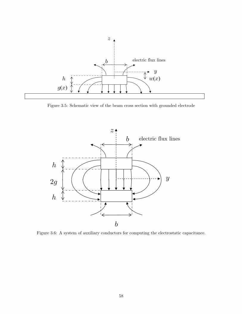
z
y
b
h
g(x)
w(x)
electric flux lines
Figure 3.5: Schematic view of the beam cross section with grounded electrode
h
2g
b electric flux lines
b
h
z
y
Figure 3.6: A system of auxiliary conductors for computing the electrostatic capacitance.
58

0.5 1 1.5 2 2.51Η
0
10
20
30
40
50
Per
cent
age
Err
or
Β =0.2
parallel- plate
Palmer
Present work
Meijs- Fokkema
b= 5 hh g= 0.2 h b= 5 h
h
g= 2.5 h
(a)
0.5 1 1.5 2 2.51Η
0
20
40
60
80
Per
cent
age
Err
or
Β =2.
parallel- plate
Palmer
Present work
Meijs- Fokkema
b= 0.5 h
hg= 0.2 h
b= 0.5 h
h
g= 2.5 h
(b)
Figure 3.7: Taking the capacitance computed with the method of moments as reference, comparisonof the error in the capacitance per unit length for a narrow microbeam obtained with differentmethods: (a) β = 0.2; (b) β = 2.
59

Figure 3.8: Schematics of the 3D FE mesh used for simulations of the clamped-clamped beam byANSYS. The domain in light grey (discretized with tetrahedral elements) is the dielectric, the onein dark grey (discretized with brick elements) is the microbeam.
60

0 200 400 600 800 1000 1200 1400V, @VoltD
-2.5
-2
-1.5
-1
-0.5
0
-ÈÈwÈÈ¥
,@Μ
mD
Σ0=100 MPa
Present work
Kuang
Osterberg
Abdel-Rahman
ANSYS
(a)
0 200 400 600 800 1000 1200 1400V, @VoltD
-2.5
-2
-1.5
-1
-0.5
0
-ÈÈwÈÈ¥
,@Μ
mD
Σ0=0 MPa
Present work
Kuang
Osterberg
Abdel-Rahman
ANSYS
(b)
0 200 400 600 800 1000 1200V, @VoltD
-2.5
-2
-1.5
-1
-0.5
0
-ÈÈwÈÈ¥
,@Μ
mD
Σ0=-100 MPa
Present work
Kuang
Osterberg
Abdel-Rahman
ANSYS
(c)
Figure 3.9: Plots of the maximum displacement versus the applied voltage for the clamped-clampedmicrobeam problem under different initial states of stress. Results from all models are reported upto their predicted pull-in instability. (a) σ0 = 100MPa; (b) σ0 = 0MPa; (c) σ0 = −100MPa.
61

0 25 50 75 100 125 150V, @VoltD
-2
-1.5
-1
-0.5
0
-ÈÈwÈÈ¥
,@Μ
mD
Present work
Osterberg, Kuang
Abdel-Rahman
ANSYS
Figure 3.10: Plot of the maximum displacement versus the applied voltage for the cantilever mi-crobeam of case (1), Table 3.2. Results from all models are reported up to their predicted pull-ininstability.
62

0 50 100 150 200 250 300
x
0
0.5
1
1.5
2
2.5
gHxL
(a)
0 20 40 60 80 100x
0
1
2
3
4
gHxL
(b)
Figure 3.11: Deformed shapes of microbeams just prior to the pull-in voltage. Dimensions along thex- and the y-axes are in µm; (a) cantilever microbeam of case (2), Table 3.2; (b) clamped-clampedmicrobeam with σ0 = 0MPa.
63
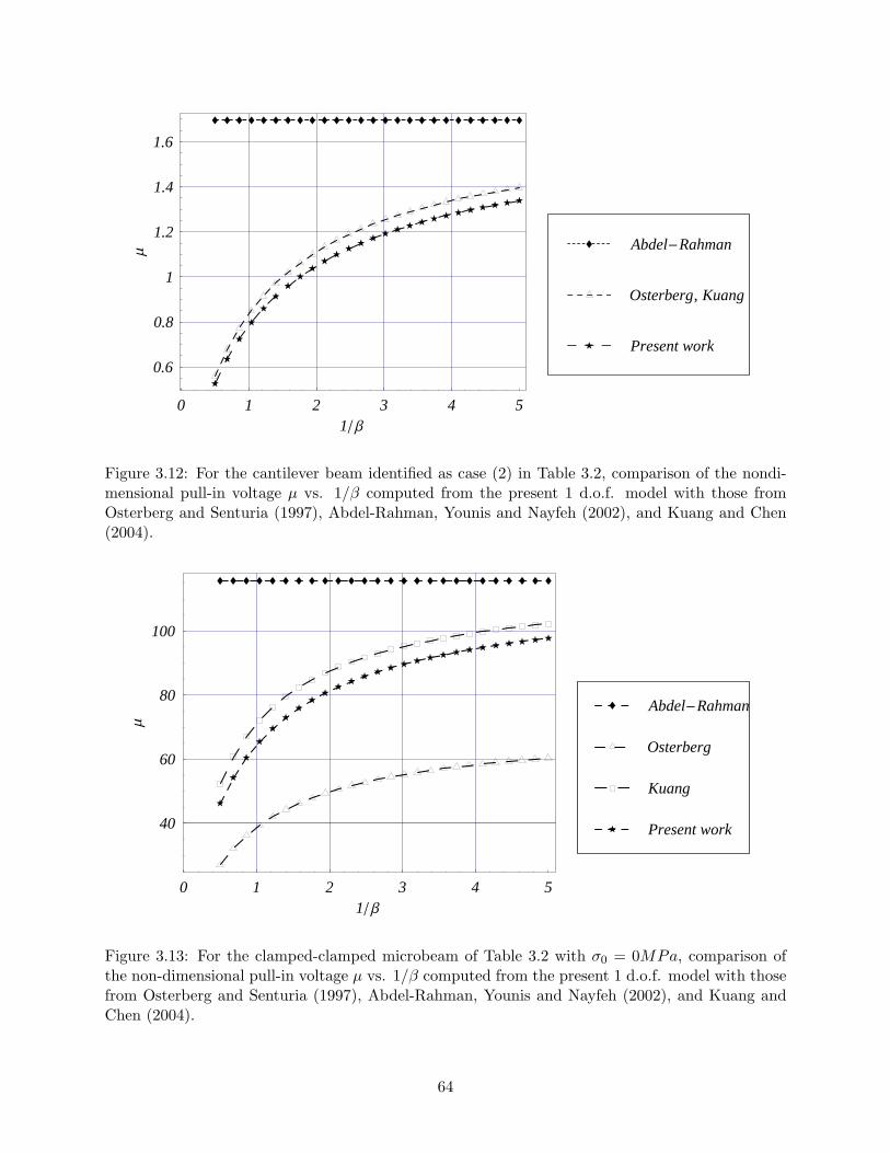
0 1 2 3 4 51 Β
0.6
0.8
1
1.2
1.4
1.6Μ
Present work
Osterberg, Kuang
Abdel-Rahman
Figure 3.12: For the cantilever beam identified as case (2) in Table 3.2, comparison of the nondi-mensional pull-in voltage µ vs. 1/β computed from the present 1 d.o.f. model with those fromOsterberg and Senturia (1997), Abdel-Rahman, Younis and Nayfeh (2002), and Kuang and Chen(2004).
0 1 2 3 4 51 Β
40
60
80
100
Μ
Present work
Kuang
Osterberg
Abdel-Rahman
Figure 3.13: For the clamped-clamped microbeam of Table 3.2 with σ0 = 0MPa, comparison ofthe non-dimensional pull-in voltage µ vs. 1/β computed from the present 1 d.o.f. model with thosefrom Osterberg and Senturia (1997), Abdel-Rahman, Younis and Nayfeh (2002), and Kuang andChen (2004).
64

0 1 2 3 4 51 Β
0.46
0.48
0.5
0.52
0.54
0.56ÈÈwÈÈ¥
Present work
Osterberg, Kuang
Abdel-Rahman
Figure 3.14: For the cantilever beam identified as case (2) in Table 3.2, comparison of the maximumpull-in non-dimensional deflection ‖w‖∞ vs. 1/β computed from the present 1 d.o.f. model withthose from Osterberg and Senturia (1997), Abdel-Rahman, Younis and Nayfeh (2002), and Kuangand Chen (2004).
0 1 2 3 4 51 Β
0.45
0.5
0.55
0.6
0.65
ÈÈwÈÈ¥
Present work
Kuang
Osterberg
Abdel-Rahman
Figure 3.15: For the clamped-clamped microbeam described in Table 3.2 with σ0 = 0MPa, compar-ison of the maximum pull-in non-dimensional deflection ‖w‖∞ vs. 1/β computed from the present1 d.o.f. model, with those from Osterberg and Senturia (1997), Abdel-Rahman, Younis and Nayfeh(2002), and Kuang and Chen (2004).
65

Chapter 4
Vibrations of Cracked Euler-BernoulliBeams
4.1 Introduction
Most load carrying systems and structures degrade or accumulate cracks during service. For
safety reasons, it is desirable that any existing cracks be detected and located before they
cause more serious damage and eventual system failure. Visual inspection is costly and te-
dious and often does not yield a quantifiable result. For some components visual inspection is
virtually impossible. Therefore, the development of structural health monitoring techniques
has received increasing attention in recent years (see, e.g., Dimarogonas (1996)). Among
these techniques, it is believed that the use of vibration data offers the most desirable alter-
native to actually dismantling the structure. In this method one excites the structure either
in free vibration or in forced harmonic oscillations and extracts the natural frequencies and,
if possible, the mode shapes. The main idea behind damage detection schemes that rely
on modal data is that a damage in the system will manifest itself as changes in the modal
characteristics.
The structural health monitoring and diagnostics generally require accurate models for the
structures, since the measured modal characteristics generally do not change much with
damage; e.g., the changes in natural frequencies due to cracks become significant only when
the structure is close to failure. As for the computational costs involved in the identification
procedure a good compromise between accuracy and simplicity should be a key feature of a
mathematical model intended to be part of the on-line health monitoring procedure. There-
fore in the last two decades, several investigators have been working on the development of
reliable and robust mathematical models of damaged structural elements, especially slender
Material in this Chapter is part of the paper “Vibrations of Cracked Euler-Bernoulli Beams Using Meshless LocalPetrov-Galerkin (MLPG) Method,” appeared in CMES: Computer Modeling in Engineering & Sciences.
66

beams. The different theoretical modeling techniques for cracked slender structures can be
grouped in two basic categories: i) “lumped flexibility” models; and ii) “continuous” models.
The first category is based on the representation of a crack as a lumped flexibility element
(generally a spring), without affecting the modeling of the undamaged regions (see, e.g.,
Gudmunson (1983), and Chondros and Dimarogonas (1998) for modeling aspects; Osta-
chowicz and Krawczuk (1991), and Khiem and Lien (2004) for a multiple cracks scenario;
and Rizos, Aspragathos and Dimarogonas (1988) for the damage identification). The de-
termination of the equivalent lumped stiffness is usually performed in the framework of
classical fracture mechanics, starting from the knowledge of the stress intensity factors. On
the other hand, the basic idea behind the second modeling strategy is to obtain a contin-
uous, one-dimensional model of the cracked beam at the level of approximation of classical
beam theory (see, e.g., Christides and Barr (1984) for modeling aspects; Shen and Pierre
(1990, 1994) for computational insights; Chondros and Dimarogonas (1998), and Chondros
(2001) for comparisons between the lumped flexibility and the continuous models; Carneiro
and Inman (2002) for the derivation of a continuous model including shear deformations).
The governing equations of the one-dimensional cracked beam are derived via a variational
principle, e.g. the Hu-Washizu-Barr method. The modification of the stress field induced by
the crack is incorporated through a local empirical function which assumes an exponential
decay with the distance from the crack. This additional crack function can be determined
in several ways, but none of them seems to be satisfactory. The adopted techniques range
from crude numerical analysis to experimental investigations passing through qualitative
fracture mechanics. For a complicated structure with multiple cracks, the solution of the
governing equations of motion requires numerical techniques, e.g. the finite element method
(Gounaris and Dimarogonas (1988), and Gounaris, Papadoupolos and Dimarogonas (1996))
or the Myklestad approach of Mahmoud, Zaid and Al Harashani (1999).
In the development of these theoretical models, it is assumed that the crack remains open
during the vibration period. However, unless a static preload exists, during vibrations of
the beam the state of stress in the cracked section varies from tension to compression, i.e.
the crack opens and closes with time. This results in a modification of the crack section
stiffness, the extremal values being the stiffness of the open crack and that of the intact
beam. Thus, the non-linear behavior of the closing crack introduces characteristics of the
non-linear systems. However, for many practical applications, the system can be considered
bilinear, and the fatigue crack can be introduced in the form of the so-called “breathing
crack” model which opens when the normal strain near the crack tip is positive, otherwise
it closes. The vibration of a beam with a closing crack has been studied in several works: in
Chondros and Dimarogonas (2001), and Shen and Chu (1992) a continuous cracked beam
theory is assumed and Galerkin procedures are applied; in Sundermeyer and Weaver (1995) a
67

lumped flexibility theory is used and analytical solutions are presented; in Qian, Gu and Jiang
(1990), Ruotolo, Surace, Crespo and Storer (1996), and Pugno, Surace and Ruotolo (2000)
a finite element model of the cracked beam is used, where reduced stiffness of an element
accounts for the crack’s presence by “smearing” the crack effect on an entire element; in
Luzzato (2003) a “smeared crack” model is compared with a finite element solution of a
lumped flexibility model.
In the present Chapter we propose an accurate numerical technique for the analysis of a beam
with multiple cracks based on MLPG6 formulation, that is, the trial and test functions are
chosen from the same space. Adopting the lumped flexibility approach, each fatigue crack is
modelled as a rotational spring and several damage scenarios are addressed. We study the
modal characteristics of a beam with multiple open cracks and its transient behavior when
the cracks are breathing.
Recent literature (Atluri, Cho and Kim (1999), and Raju and Phillips (2003)) shows in-
creasing interest in the analysis of beams by the use of MLPG methods. In Atluri, Cho and
Kim (1999) the static analysis of thin beams is presented using the MLPG6 method. In
particular, the conventional Moving Least Squares (MLS) approximation presented in Lan-
caster and Salkauskas (1981) is generalized to treat 4-th order boundary value problems, and
the resulting Generalized Moving Least Squares (GMLS) approximation is used to construct
simultaneously the test and trial functions. In Raju and Phillips (2003) the static analysis
of thin beams is addressed by the use of a Petrov-Galerkin implementation of the MLPG
method, where the trial functions are constructed using the GMLS approximation and the
test functions are chosen from a different space. The GMLS basis functions are generally
continuously differentiable over the entire domain which results in continuous derivatives of
the trial solution. Thus the treatment of cracked beams necessitates the use of special tech-
niques to account for the slope discontinuities at the crack stations (a similar problem has
been studied in Batra, Porfiri and Spinello (2004) for heat conduction in a bimaterial body).
In the present chapter we use the MLPG6 variant and adopt a substructure approach, by
making use of Lagrange multipliers to model the spring effects at the crack locations and
relate deformations of the intact beam segments. Warlock, Ching, Kapila and Batra (2002)
employed the method of Lagrange multipliers to enforce traction boundary conditions at a
contact surface.
The rest of the Chapter is organized as follows. In Section 4.2 we study the dynamics of
a multiply cracked beam with the MLPG method. The presence of cracks is accounted
for by the introduction of suitable Lagrange multipliers, which guarantee the deflection
continuity at the crack locations. The static deformations, the transient behavior, and the
modal properties are considered in the analysis. The stability of the mixed formulation is
discussed, and the inf-sup condition is proved. In Section 4.3 we consider effects of cracks
68

opening and closing during the beam vibration period; i.e., we consider the transient analysis
of a beam with breathing cracks. In Section 4.4 we report results of numerical experiments,
and compare present results with those from other numerical methods, exact solutions and/or
experimental findings. Indeed, we compare the finite element and meshless methods in the
analysis of static deformations and in the estimation of the modal properties, and we compare
the meshless method with the method proposed in Sundermeyer and Weaver (1995) for the
analysis of the transient deformations of a beam with breathing cracks. For the sake of
brevity, the approach is presented for a simply supported beam, although it has been found
suitable also for other boundary conditions. A description of the GMLS approximation is
found in Appendix A.2
4.2 Vibrations of a multiply cracked beam
4.2.1 Governing equations
A beam of length l, cross-sectional area A = h × b, moment of inertia I = bh3/12, Young’s
modulus E, mass density per unit volume ρV , and with n cracks located at points c1,..., cn is
considered. The simplest way to account, with a reasonable accuracy, for effects of cracks on
the dynamic properties of a slender beam is to represent cracks as lumped flexibility elements
and to model the intact regions as Euler-Bernoulli beams. Therefore, following Gudmunson
(1983), and Chondros and Dimarogonas (1998), cracks are modeled as n massless rotational
springs whose stiffnesses are denoted by k1, . . . , kn As a consequence, we divide the beam
into n + 1 sub-intervals Ωi = [ci−1, ci] (c0 ≡ 0, and cn+1 ≡ l) of length li, introduce the
n + 1 local abscissas ξi, and consider n + 1 deflection fields wi (ξi) . Figure 4.1 exhibits the
geometry of the cracked beam.
The vibrations of each undamaged beam segment are governed by
KMwIVi (ξi, t) + ρ wi (ξi, t) = pi (ξi, t) , ξi ∈ (0, li) , t > 0, (4.1)
where the rotatory inertia has been neglected, ρ = ρV A is the linear mass density, KM = EI
is the bending stiffness, pi (ξi, t) is an applied distributed transverse load, and a superimposed
dot means time derivative. The boundary conditions for the generic i− th subinterval are
wi (li, t) = wi+1 (0, t) , w′′i (li, t) = w′′
i+1 (0, t) ,
w′′′i (li, t) = w′′′
i+1 (0, t) , w′′i (li, t) = − ki
KM
(w′
i+1 (0, t)− w′i (li, t)
) . (4.2)
For the two boundary elements Ω1 and Ωn+1 the following additional constraints are imposed:
69

w1 (0, t) = 0, w′′
1 (0, t) = 0,wn+1 (ln+1, t) = 0, w′′
n+1 (ln+1, t) = 0. (4.3)
Following Chondros and Dimarogonas (1998), values of the rotational spring constants ki
can be found from the section geometry, the crack depth ai, and the material properties:
ki =1
αi
, αi =6π (1− ν2)
EIIc
(ai
h
), (4.4)
where ν is the Poisson ratio and
Ic (z) = 0.6272 z2 − 1.04533 z3 + 4.5948 z4 − 9.9736 z5 + 20.2948 z6+
− 33.0251 z7 + 47.1063 z8 − 40.7556 z9 + 19.6 z10, (4.5)
with z indicating severity of the i-th crack. This modeling technique provides reasonable
results as long as cracks remain open during the vibration period. The crack opening and
closing (breathing crack) introduce weak non-linearities in the beam motion, and modify
natural frequencies of vibrations. In the following Section we analyze the effect of breathing
cracks by a meshless method together with a classical time integration scheme.
4.2.2 Semi-discrete formulation
In order to derive a weak formulation of the aforementioned fourth-order problem suitable
for numerical methods, we introduce the augmented Lagrangian that is a function of the
deflection fields wi in the undamaged beam segments, and the Lagrange multipliers λi:
L (w1, ..., wn+1, λ0, ..., λn+1) =
1
2
n+1∑i=1
∫ li
0
[ρ w2
i −KM (w′′i )
2+ 2piwi
]dξi − 1
2
n∑i=1
ki
(w′
i+1 (0)− w′i (li)
)2−n∑
i=1
λi (wi+1 (0)− wi (li))− λ0w1 (0)− λn+1wn+1 (ln+1) , (4.6)
where we have omitted the dependence on time of the deflection fields, Lagrange multipli-
ers and of the applied load. The Lagrange multipliers λ0 and λn+1 are used to impose the
displacement boundary conditions at the ends, while the other Lagrange multipliers impose
70

the continuity of deflections at the crack locations. We emphasize that the proposed formu-
lation leads to continuous deflections along the entire beam span. On the other hand, the
continuity of the bending moments and of the shear forces at the crack locations are satisfied
only approximately. By extremizing the Action on the set of isochronous motions we obtain
n+1∑i=1
∫ t
0
∫ li
0
[ρ wi δwi + KMw′′i δw
′′i − piwi] dξidt+
n∑i=1
ki
(w′
i+1 (0)− w′i (li)
) (δw′
i+1 (0)− δw′i (li)
)+
∫ t
0
[λ0δw1 (0) + λn+1δwn+1 (ln+1) +
n∑i=1
λi (δwi+1 (0)− δwi (li))
]dt+
∫ t
0
[δλ0w1 (0) + δλn+1wn+1 (ln+1) +
n∑i=1
δλi (wi+1 (0)− wi (li))
]dt = 0. (4.7)
Next, we consider n + 1 distinct sets of scattered points Ni =
ξi1 , ..., ξiNi
with ξi1 = 0,
ξiNi= li = ξ(i+1)1
, for the subintervals Ωi, and derive independently n+1 distinct set of basis
functions ψi (ξi) of the type (A.28). We denote with N the total number of nodes scattered
on the entire beam, and we emphasize that at each crack location two overlapping nodes are
placed. For convenience, these trial functions are derived by assuming for each subinterval
the same order for the monomial basis functions in the GMLS approximation and the same
form of the weight functions (A.29). Furthermore, we denote by Rij the radius of the support
of the j-th weight function of the i-th subdomain. We consider test functions of the form:
δwi = ψTi (ξi) µi, (4.8)
where µi is a 2Ni-vector of arbitrary constants.
By substituting in (4.7) the GMLS approximation together with the considered test func-
tions, and by accounting for the arbitrariness of the real constants µi’s we obtain the following
semi-discrete formulation
M
··s + Ks + Λλ = F
ΛTs = 0. (4.9)
The generalized displacement vector is comprised of nodal displacements and rotations in
all segments of the beam:
71

s =[
s1 · · · si · · · sn+1
]T. (4.10)
The mass matrix M is a symmetric nonnegative definite block diagonal matrix
M =
m1 0 · · · 00 m2 0 · · ·· · · 0 · · · · · ·0 · · · · · · m(n+1)
, (4.11)
with
mi = ρ
∫
Ωi
ψi (ψi)T dξi. (4.12)
Therefore, the beam segments are inertially uncoupled by the lumped flexibilities appearing
in the cracked beam model but are elastically coupled.
The symmetric nonnegative definite stiffness matrix can be decomposed as
K = K0+n∑
i=1
Kspri , (4.13)
where the block-diagonal stiffness contribution K0 is obtained from the segments’ stiffness
matrices following the same procedure as that used for assembling of M from the segments’
mass matrices:
K =
k1 0 · · · 00 k2 0 · · ·· · · 0 · · · · · ·0 · · · · · · k(n+1)
, (4.14)
with
ki = KM
∫
Ωi
(ψi)′′ ((ψi)
′′)Tdξi. (4.15)
On the other hand, the contribution of the i-th crack to the beam stiffness Kspri has non-zero
entries only in correspondence with the i-th and (i + 1)-th beam segments, i.e.:
72

Kspri =ki
0 · · · · · · · · · · · · 0· · · · · · · · · · · · ... · · ·· · · · · · Ai Bi · · · · · ·· · · · · · BT
i Ci · · · · · ·· · · · · · · · · · · · · · · · · ·0 · · · · · · · · · · · · 0
, (4.16)
where matrices Ai, Bi and Ci are given by
Ai = (ψi)′ (li)
((ψi)
′ (li))T
,
Bi = − (ψi)′ (li)
((ψi+1)
′ (0))T
,
Ci = (ψi+1)′ (0)
((ψi+1)
′ (0))T
.
(4.17)
The constraint matrix Λ is assembled by appending the column vectors
Λ =[
Λ0 Λ1 · · · Λi · · · Λn Λn+1
], (4.18)
where
Λ0 =
a0
0· · ·0
, Λi =
0· · ·ai
bi
0· · ·0
, Λn+1 =
00· · ·
bn+1
. (4.19)
The column vectors with subscripts 0 and n + 1 arise from the need to satisfy displacement
boundary conditions, while the one with subscript i is due to the i-th crack. The subvectors
are related to the test and the trial functions as
a0 = ψ1 (0) , ai = −ψi (li) , bi = ψi+1 (0) , bn+1 = ψn+1 (ln+1) . (4.20)
Finally, the force vector F is given by
F =[
f1 · · · fi · · · fn+1
]T, (4.21)
with
73

fi =
∫
Ωi
piψidξi. (4.22)
4.2.3 Inf-sup test
In order to achieve a stable and optimal procedure for the MLPG method employing a set of
Lagrange multipliers, the considered mixed formulation for static problems should satisfy the
ellipticity condition (on the space of displacements fields satisfying the kinematic boundary
conditions) and the inf-sup condition (see, e.g., Bathe (1996)). For this linear problem the
ellipticity condition is readily satisfied, while additional effort is needed to provide criteria
for satisfying the inf-sup condition, which reads:
infλ∈IRn+2/0
supwh∈W h/0
λ0wh1 (0) +
n∑i=1
λi
(wh
i+1 (0)− whi (li)
)+ λn+1w
hn+1 (ln+1)
‖λ‖ ‖wh‖ ≥ β > 0, (4.23)
where β is a constant independent of the nodal locations, and W h ⊂ H2 (0, l1)×...×H2 (0, ln)
is the GMLS solution space. The norm of the approximate deflection field is defined by
∥∥wh∥∥2
=n+1∑i=1
∫ li
0
[(wh
i
)2+ l2
((wh
i
)′)2
+ l4((
whi
)′′)2]
dξi, (4.24)
while the norm of the vector of scalars λ is given by
‖λ‖2 = λTλ. (4.25)
When these two conditions are satisfied, the stability of the MLPG formulation is guaranteed,
and optimal error bounds are obtained for the chosen GMLS solution.
We show below that the inf-sup condition is satisfied when m, the order of the monomial
basis in (A.20), is greater than 1. Indeed, in this case the GMLS approximation is able to
exactly reproduce affine functions (see (A.21) when a (x) is a constant). Therefore, for a
typical λ, we choose deflection fields of the form
whi (ξi) = λi−1
(1− ξi
li
), i = 1, ..., n
whn+1 (ξi) = λn +
λn+1 − λn
ln+1
ξn+1
. (4.26)
74

The norm of this deflection is easily computed as:
∥∥wh∥∥2
=n+1∑i=1
λ2i−1
(li3
+l2
li
)+ λ2
n+1
(ln+1
3+
l2
ln+1
)+ λn+1λn
(ln+1
3− 2
l2
ln+1
). (4.27)
Equation (4.27) may be alternatively rewritten in matrix notation as:
∥∥wh∥∥2
= λTSλ, (4.28)
where the (n + 2, n + 2) matrix S defined by
S =
(l13
+ l2
l1
)0 · · · · · · 0
0(
l23
+ l2
l2
)0 · · · 0
· · · 0 · · · · · · · · ·0 0 0
(ln+1
3+ l2
ln+1
)12
(ln+1
3− 2 l2
ln+1
)
0 · · · · · · 12
(ln+1
3− 2 l2
ln+1
) (ln+1
3+ l2
ln+1
)
, (4.29)
appears. The eigenvalues σ1, ..., σn+2 of S are:
σi =
(li3
+l2
li
), i = 1, ..., n, (4.30)
σn+1 =ln+1
2, σn+2 =
ln+1
6+ 2
l2
ln+1
. (4.31)
Hence S is a positive definite matrix, and
max σi ‖λ‖2≥∥∥wh
∥∥2≥min σi ‖λ‖2 . (4.32)
By substituting (4.26) in the argument of the inf-sup we obtain
λ0wh1 (0) +
n∑i=1
λi
(wh
i+1 (0)− whi (li)
)+ λn+1w
hn+1 (ln+1)
‖λ‖ ‖wh‖ =‖λ‖√λTSλ
. (4.33)
Hence, we have
75

supwh∈W h/0
λ0wh1 (0) +
n∑i=1
λi
(wh
i+1 (0)− whi (li)
)+ λn+1w
hn+1 (ln+1)
‖λ‖ ‖wh‖ ≥ ‖λ‖√λTSλ
(4.34)
with λ still a variable. Therefore, for the mixed GMLS approximation with m > 1 we have
infλ∈IRn+2/0
supwh∈W h/0
λ0wh1 (0) +
n∑i=1
λi
(wh
i+1 (0)− whi (li)
)+ λn+1w
hn+1 (ln+1)
‖λ‖ ‖wh‖ ≥
infλ∈IRn+2/0
‖λ‖√λTSλ
=1√
max σi
, (4.35)
and the inf-sup condition is satisfied.
4.2.4 Modal analysis
The natural frequencies and mode shapes of the undamaged beam are obtained by searching
for solutions of the type
s (t) = s exp (iωt) , λ (t) = λ exp (iωt) , (4.36)
of (4.9) and by discarding the applied loads. Therefore, the following eigenvalue problem
arises:
−ω2Ms + K s + Λλ = 0ΛTs = 0
. (4.37)
The second equation in (4.37) provides 2 + n constraints on the mode shapes s.We modify
the eigenvalue problem (4.37) so that the imposed constraints are automatically satisfied.
Let us consider the null space of ΛT, denoted by kerΛT. When the inf-sup condition is
satisfied the dimension of the kernel of ΛT is
dim kerΛT = (2N − 2− n) , (4.38)
since 2 + n Lagrange multipliers appear in this formulation and the system is solvable (see,
e.g., Bathe (1996) for a discussion of the relations between solvability and stability con-
ditions). Next, we introduce the matrix Y whose columns constitute a basis for kerΛT,
76

the dimensions of Y are (2N × (2N − 2− n)). By using the rectangular matrix Y we can
express the generic modal shape s in terms of the reduced (2N − 2)-dimensional vector x by
s = Yx, (4.39)
and automatically satisfy the second equation in (4.37).
Premultiplying the first equation in (4.37) by YT and by taking into account (4.39) we obtain
the reduced system
−ω2M∗ x + K∗ x = 0, (4.40)
where
M∗= YTMY, K∗ = YTKY. (4.41)
Next, we solve for x, and obtain the complete vector of unknowns using (4.39). We note that
the kinematical boundary conditions are satisfied by the introduction of Lagrange multipliers,
while the natural boundary conditions are satisfied only in the weak sense. Furthermore we
can always assume that
YTY = 1, (4.42)
by choosing orthonormal basis for the null space of ΛT. We note that the mass and the
stiffness matrices of the reduced system are symmetric and positive definite.
4.2.5 Free motion
We integrate the differential equations of motion (4.9) with initial conditions
s (0) = s0·s (0) =
·s0
(4.43)
satisfying the boundary conditions
ΛTs0 = 0, ΛT·s0 = 0, (4.44)
77

and vanishing external load, by applying the Newmark family of methods (see, e.g., Hughes
(2001)) to the reduced system
M∗ ··x + K∗ x = 0, (4.45)
with initial conditions: x (0) = YTs0
·x (0) = YT
·s0
. (4.46)
This family of algorithms consists of the following recursive relations:
M∗an+1 + K∗xn+1 = 0,
xn+1 = xn + ∆tvn +∆t2
2[(1− 2β) an + 2βan+1] ,
vn+1 = vn + ∆t [(1− γ) an + γan+1] ,
(4.47)
where an, vn and xn are approximations of··x (tn) ,
·x (tn) and x (tn) respectively, ∆t is the
time step, and β and γ are parameters.
4.3 Effects of crack opening and closing
During the vibration period of a cracked beam, the n cracks will open and close in time
depending on the vibration amplitude. In order to model the effects of the cracks opening
and closing, we consider a bilinear behavior of each crack. When the i-th crack is open, the
i-th and (i + 1)-th beam segments are elastically coupled by the rotational spring ki (see the
continuity conditions (4.2). On the other hand, when the i-th crack is closed, the i-th and
(i + 1)-th beam segments are rigidly connected, and the boundary conditions become
wi (li, t) = wi+1 (0, t) , w′′i (li, t) = w′′
i+1 (0, t) ,w′′′
i (li, t) = w′′′i+1 (0, t) , w′
i (li, t) = w′i+1 (0, t) .
(4.48)
The i-th single edge crack is assumed to be open or closed depending on the sign of the
curvature w′′i+1 (0, t):
• if the crack is on the upper beam surface, the crack is open when the curvature is
negative and vice-versa,
• if the crack is on the bottom beam surface, the crack is open when the curvature is
positive and vice-versa.
78

When the i-th crack is closed the augmented Lagrangian (4.6) needs to be modified by
removing the strain energy contribution from the spring ki, and by introducing an additional
Lagrange multiplier ζi to enforce the continuity of rotations at the crack location. Therefore,
the equations of motion of the cracked beam are
M··s + K0s+
n∑i=1
δiKspri s + Λλ+
n∑i=1
(1− δi)Υiζi= 0,
ΛTs = 0,(1− δi)Υ
Ti s = 0, i = 1, ...n,
(4.49)
where δi is equal to 1 or 0 if the i-th crack is open or closed. The new vector Υi is given by
Υi =[
0 · · · ci di 0 · · · 0]T
, (4.50)
where the subvectors are decomposed by:
ci = − (ψi)′ (li) , di = (ψi)
′ (0) . (4.51)
If q cracks are closed, the number of Lagrange multipliers is 2 + n + q, and the third set of
equations in (4.49) consists of q equations.
The instantaneous values of the δ’s depend on the sign of curvature at the crack locations.
The aforestated weak formulation does not guarantee continuity of the curvature along the
beam span. Therefore, the generic δi can be estimated either from the average curvature at
the i-th crack location, or from the curvature of any of the two segments.
Vibration cycle is referred to as the time interval between two consecutive sign changes in
the curvature at any crack location; the so-called transition time separates two consecutive
vibration cycles. During each vibration cycle, labelled by the index τ , the time integration
of the non-linear equations of motion can be performed by applying the Newmark family of
methods to the reduced equations during the τ -th cycle:
M∗τ
··xτ (t) + K∗
τ xτ (t) = 0. (4.52)
The set (4.52) of linear ordinary differential equations with constant coefficients has been
obtained with the same procedure as that used for open cracks, provided that the actual
constraints are accounted for during the current vibration cycle τ. Numerical integration gives
estimates of transition times only within the accuracy of the time step ∆t. If a transition
occurs in between the J and J + 1 integration steps, which separate the vibration cycles τ
79

and τ + 1, then the the initial conditions for the τ + 1 vibration cycle can be derived as
follows:
xτ+1 (tJ+1) = Yτ+1
TYτxτ (tJ+1)vτ+1 (tJ+1) = Yτ+1
TYτvτ (tJ+1), (4.53)
where columns of the matrix Yτ constitute an orthonormal basis for kerΛTτ . The left-hand
side of (4.53) are the projection of the solution xτ and vτ on the basis of the solution at the
subsequent cycle xτ+1 and vτ+1.
4.4 Computation and discussion of results
For investigating the characteristics of the proposed method, several tests are performed on
the sample problem of a simply supported beam with a single crack located at the mid-span.
When the beam is subjected to a constant distributed load p, the static deflection is
w1 (ξ1) =pl2 (2k1l + 3KM)
48KMk1
ξ1 − pl
12KM
ξ31 +
p
24KM
ξ41
w2 (ξ2) =pl3 (5k1l + 12KM)
384KMk1
− pl2
16k1
ξ2 − pl2
16KM
ξ22 +
p
24KM
ξ42
. (4.54)
The exact modal properties of a beam with one open crack are given in Sundermeyer and
Weaver (1995). The odd natural frequencies are roots of the trascendental characteristic
equation:
−4k1
KM
cos
(lβ
2
)+ β
(sin
(lβ
2
)− cos
(lβ
2
)tanh
(lβ
2
))= 0, (4.55)
while the even ones are
β =rπ
l, r = 2, 4, 6, .... (4.56)
The odd mode shapes are
w1 (ξ1) = A [sin (βξ1) + α sinh (βξ1)] ,
w2 (ξ2) = A
[sin
(β
(l
2− ξ2
))+ α sinh
(β
(l
2− ξ2
))],
α =
cos
(lβ
2
)
cosh
(lβ
2
) , (4.57)
80

while the even ones are
w1 (ξ1) = A sin (βξ1)w2 (ξ2) = A sin (β (ξ2 − l/2))
. (4.58)
The constant A is chosen by ensuring that∫ l/2
0
(w1 (ξ1))2 dξ1 +
∫ l/2
0
(w2 (ξ2))2 dξ2 = 1. (4.59)
The GMLS basis functions are generated by complete monomials of degree 2 (m = 3). This
choice is motivated by the need of satisfying the inf-sup condition, guaranteeing an accurate
GMLS reconstruction, and of reducing the computational time. For m = 3 the GMLS trial
functions require the inversion of a 3 × 3 matrix, which can be done analytically once for
all. Every beam segment is discretized with the same number of nodes N1 = N2, and the
nodal spacing is uniform. The radius of support of each weight function is the same and
equals sl1/ (N1 − 1) = sl2/ (N2 − 1) , where s is the ratio between the weight function radius
and the distance between two adjacent nodes. In order to achieve smooth approximate
solutions, the power α in (A.29) is set equal to 5. Increasing the order of differentiability of
the weight functions does not lead to additional computational effort, therefore it is generally
advisable to exploit high values of α. The numerical integrations needed for computing the
stiffness matrix, the mass matrix, and the load vector are performed using the non-element
local technique described in Atluri, Cho and Kim (1999) with 10 quadrature points in each
subregion of intersection of sub-domains.
We compare the MLPG results with those obtained from the traditional Finite Element
method (FEM), which may be directly derived upon replacing the GMLS approximation
with the Hermitian interpolation function (see, e.g., Hughes (2001)) in the stiffness matrix,
in the mass matrix, and in the force vector. We emphasize that within the FEM there
is no need to use a mixed formulation based on the introduction of Lagrange multipliers
for prescribing the boundary and the interface conditions. The trial functions of the FEM
possess the Kronecker Delta property and the constraints are simply imposed by eliminating
from the stiffness matrix, the mass matrix, and the force vector the entries corresponding to
constrained nodes.
We analyze deformations of an aluminum beam with following values of material and geo-
metric parameters:
E = 72 Gpa, ρV = 2800 kg/m3, ν = 0.35, l = 235 mm,
h = 23 mm, b = 7 mm, a1 = 0.4h. (4.60)
81
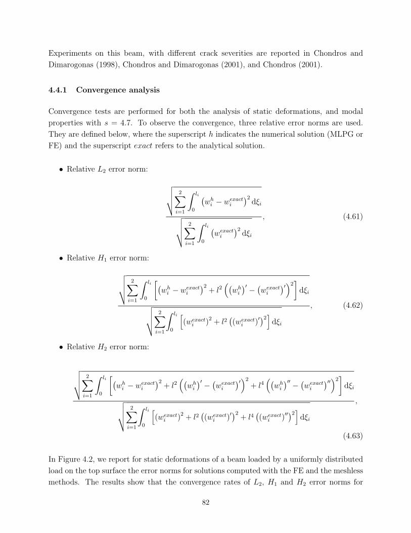
Experiments on this beam, with different crack severities are reported in Chondros and
Dimarogonas (1998), Chondros and Dimarogonas (2001), and Chondros (2001).
4.4.1 Convergence analysis
Convergence tests are performed for both the analysis of static deformations, and modal
properties with s = 4.7. To observe the convergence, three relative error norms are used.
They are defined below, where the superscript h indicates the numerical solution (MLPG or
FE) and the superscript exact refers to the analytical solution.
• Relative L2 error norm:
√√√√2∑
i=1
∫ li
0
(wh
i − wexacti
)2dξi
√√√√2∑
i=1
∫ li
0
(wexact
i
)2dξi
, (4.61)
• Relative H1 error norm:
√√√√2∑
i=1
∫ li
0
[(wh
i − wexacti
)2+ l2
((wh
i
)′ − (wexact
i
)′)2]
dξi
√√√√2∑
i=1
∫ li
0
[(wexact
i )2 + l2((wexact
i )′)2
]dξi
, (4.62)
• Relative H2 error norm:
√√√√2∑
i=1
∫ li
0
[(wh
i − wexacti
)2+ l2
((wh
i
)′ − (wexact
i
)′)2
+ l4((
whi
)′′ − (wexact
i
)′′)2]
dξi
√√√√2∑
i=1
∫ li
0
[(wexact
i )2 + l2((wexact
i )′)2
+ l4((wexact
i )′′)2
]dξi
,
(4.63)
In Figure 4.2, we report for static deformations of a beam loaded by a uniformly distributed
load on the top surface the error norms for solutions computed with the FE and the meshless
methods. The results show that the convergence rates of L2, H1 and H2 error norms for
82

the two methods are almost the same and approximately equal 4, 3 and 2 respectively. In
general, the error of the MLPG solution is lower than that of the FE solution.
Figure 4.3 shows the relative errors in the resonance frequencies of the three lowest vibration
modes. Also in this case, the convergence rates for the two methods are almost the same
and approximately equal 4. Nevertheless, it may be seen that the magnitude of the error
obtained with the meshless approach is less than that with the FEM.
Figures 4.4, 4.5 and 4.6 show, respectively, the convergence rates of L2, H1 and H2 error
norms for the three lowest modes computed with the two numerical methods. The results
show that, also in this case, the convergence rates of L2, H1 and H2 error norms for the
two methods are almost the same and approximately equal 4, 3 and 2 respectively. The
magnitude of the error in the highest modes achieved with the MLPG method is still lower
than that obtained with the FEM.
4.4.2 Variations of weight functions radii
From the above analysis, it is evident that when increasing the number of nodes the MLPG
method tends to reach a stable convergence rate similar to the FEM. On the other hand
when only a few nodes are employed non monotonic behaviors are exhibited and the MLPG
solution is more accurate than the FE solution (see, e.g., Figure 4.3). This is due to the fact
that for coarse grids the local feature of the MLPG method is lost and each node is affecting
almost all nodes, increasing the computational time for evaluating every matrix entry but
also considerably improving the accuracy of the GMLS reconstruction capability.
Here we investigate the behavior of the MLPG solution when the number of nodes in each
segment is kept constant (4 nodes per segment) while the radius of the weight functions is
increased until each node is affecting all the other ones (1.5 ≤ s ≤ 4).
Figure 4.7 shows the error in the static deflection computed with the MLPG and the FE
methods. It is clear that increasing the radius of the weight functions leads to a significant
improvement of the MLPG solution. Indeed, for s ≤ 3 the FE solution is more accurate
than the MLPG one, but when s > 3 the situation is completely reversed and the MLPG
method gives significantly less errors than the FEM.
Figure 4.8 shows the four lowest natural frequencies computed with the MLPG and the
FE methods. Also in this case, an increase in the weight functions radii leads to a great
improvement. Whereas, the error in the first natural frequency monotonically decreases with
an increase in the parameter s, the errors in other frequencies do not decrease monotonically;
however, they are always much lower (about 100 times) than those for the FE solution.
In Figure 4.9 we report the exact ratio of the first natural frequency of the intact beam to that
83

of the cracked beam for different values of the crack depth a (solid line) and its approximation
by using the 4 + 4 nodes configuration with s = 3. The open circles indicate experimental
values from either Chondros and Dimarogonas (1998) or Chondros (2001). It is clear that the
computed values agree very well with the analytical ones; however, the two differ somewhat
from the experimental values. This may be due to an inaccurate mathematical model or
to unrefined experimental measurements. Nevertheless, the experimental program aimed at
validating the lumped flexibility conducted first in Gudmunson (1983) on cracked cantilever
beams validates the mathematical model and suggests that the discrepancies are due to
experimental errors. A possible source of errors is the realization of the hinges for the
vibration testing of the simply supported beam. Indeed, from the experimental viewpoint,
the realization of hinges represents a much more challenging problem than fixing the edges.
Furthermore, while the quoted experimental tests of Gudmunson (1983) were conducted on
beams cracked by saw-cuts, those of Chondros and Dimarogonas (1998), and of Chondros
(2001) refer to fatigue cracks. It is well known that the controlled introduction of fatigue
cracks involves several experimental difficulties not encountered in the saw cut method.
4.4.3 Transient analysis for a breathing crack
Here, we analyze free vibrations of the cracked beam when the crack is assumed to breath.
We assume that the crack is located on the lower surface of the beam, the beam is initially
undeformed and is excited according to the first mechanical mode shape of the intact beam.
The nonlinearity introduced by the bilinear behavior of the breathing crack does not allow
for a simple analytical solution of the transient problem.
Accordingly, we compare our results with those obtained by the algorithm of Sundermeyer
and Weaver (1995). The technique in Sundermeyer and Weaver (1995) relies on the a priori
knowledge of the mode shapes of the intact beam and of the beam with the open crack,
and consists of consecutive calculations of the beam mode amplitudes. At each vibration
cycle the deflection is expressed in terms of a finite number of mode shapes: if the crack
is closed the modal shapes of the intact beam are used, otherwise the mode shapes of the
cracked beam in (4.57) and (4.58) are used. The transition times between the two crack
states are determined by continuously monitoring the sign of the curvature at the crack
location. The initial conditions for free oscillations at each vibration cycle are determined
by simply converting the sets of natural coordinates at the transition times. We note that at
the instants of crack opening and closing, several concomitant mode shapes may arise since
the mode shapes of the intact and the cracked beam are in general not orthogonal.
The numerical integration of governing equations (4.52) is performed by using the 4 + 4
nodes configurations described in the previous subsection with s = 3 and the damped un-
84

conditionally stable Newmark integration scheme (see, e.g., Hughes (2001)) with
β = 0.3025, γ = 0.6, ∆t = 1.04 µs. (4.64)
This choice of parameters introduces a small numerical damping, which rapidly damps out
undesired oscillations at the transition instants. The transition times are computed by
continuously monitoring the average curvature at the crack location: i.e., the average of the
curvatures of the two beam segments at the crack location.
In Figure 4.10 we compare the time evolution of the deflections at the crack station computed
with the proposed technique and that presented in Sundermeyer and Weaver (1995) with
25 mode shapes. Figure 4.11 compares the time history of the relative rotation at the crack
station computed with the two methods. It is evident that the solution with the MLPG
method agrees very well with that given in Sundermeyer and Weaver (1995).
4.4.4 Remarks
As is rather well known, Euler’s beam theory simulates well deformations of a thin beam.
For a thick beam one should employ either the Timoshenko beam theory or a higher-order
shear and normal deformable beam theory such as that proposed by Batra and Vidoli (2002).
Qian, Batra and Chen (2003a,b; 2004a,b), and Qian and Batra (2004, 2005) have studied by
the MLPG method static and dynamic deformations of both homogeneous and functionally
graded isotropic thick plates, and have compared the performance of the MLPG1 and the
MLPG6 formulations. For a thick beam one will very likely need to modify the expression
for the rotational spring constants ki in (4.2).
We have considered cracks aligned along the depth of the beam which is appropriate for
a thin beam. For cracks either parallel or inclined to the longitudinal centroidal axis of
the beam, one will need to modify the problem formulation. Ching and Batra (2001), and
Batra and Ching (2002) have applied the MLPG method to determine crack-tip fields in a
pre-cracked plate deformed either statically or dynamically.
Even though the CPU time required to compute an element of the stiffness matrix in the
MLPG6 formulation adopted here has been rather large as compared to that in the FEM,
Atluri, Han and Rajendran (2004) have shown that it is not so in their mixed MLPG formula-
tion in which both displacements and strains are interpolated with the MLS basis functions.
85

4.5 Conclusions
We have used the MLPG method to study vibrations of a cracked beam. When studying
dynamic problems for cracked beams the penalty method does not seem to be adequate
since it leads to ill-conditioned problems. Therefore, the treatment of vibrations of cracked
beams necessitates the use of Lagrange multipliers to account for the relative rotation at the
crack locations and satisfy the kinematic boundary. The accurate estimation of the relative
rotation at the crack locations is crucial for the identification process based on mode shapes
(see, e.g., Rizos, Aspragathos and Dimarogonas (1988)) and for the transient analysis of a
breathing crack (see, e.g., Sundermeyer and Weaver (1995)).
The stability of the method is assessed by analytically proving the inf-sup condition. The
MLPG method is initially applied to compute the modal characteristics (both frequencies
and mode shapes), and to analyze the transient and static deformations of beams with
multiple open cracks. The derivation of reduced systems, where the imposed constraints
are automatically satisfied, has been presented. It is also extended to treat the effects of
breathing cracks on the dynamics of a cracked beam. Each crack is modeled as a bilinear
spring with spring constant changing according to the value of the beam curvature at the
crack location. Computational details for the derivation of the initial conditions at each
vibration cycle have been provided. The numerical time integration is performed by the use
of the Newmark family of methods, and the spatial integration in the MLPG formulation
employs Gaussian quadrature.
Numerical results for a simply supported beam are presented and compared with those ob-
tained from analytical, FE and semi-analytical methods. In particular, results of the MLPG
method are compared with those of the FEM for both the static and the beam modal anal-
ysis. The convergence rates of the MLPG formulation are similar to those of the FEM,
but for a fixed number of degrees of freedom the MLPG results are generally more accurate
than the FE ones. Furthermore, the accuracy of the MLPG method may be controlled by
modifying the supports of the weight function used in the GMLS approximation. It is shown
that with few nodes and very large supports extremely accurate estimates of both the static
deformations and the modal properties may be achieved. This represents a very favorable
feature of the MLPG method with respect to the FEM. When comparing the computational
time of the MLPG method with the computational time of the FEM for a fixed number of
nodes the FEM clearly wins but, when the accuracy is also considered the comparison is
not so bad. Indeed, very few nodes in the MLPG method may be satisfactory for highly
accurate numerical solutions valid over wide frequency ranges. The possibility of using a
reduced number of degrees of freedom is desirable when analyzing transient deformations
with breathing cracks. Indeed, the use of small stiffness and mass matrices greatly alleviates
86

the computational time when solving these non-linear transient problems. The MLPG pre-
dictions are in very good agreement with those of the method of Sundermeyer and Weaver
(1995), which is based on the exact knowledge of the cracked beam mode shapes and is
difficult to extend to more complicated structures, such as cracked frames. Furthermore, the
possibility of retaining reduced order numerical models may be crucial in identification or
optimization processes when algorithms should be built based on the number of degrees of
freedom.
The present implementation of MLPG method represents an interesting alternative to the
classical FEM for the analysis of cracked beams (see Table 4.1 for a summary of comparison
between the two methods).
87

MLPG FEMWeak formulation Local GlobalInformation neededabout the nodes
Locations onlyLocations andconnectivity
SubdomainsNot necessarilydisjoint
Disjoint
Trial functions
Relatively complex anddifficult to express (GMLS)but easy to generate asclosed-form expressions
Hermite polynomials
Integration rule Higher order Lower order
Mass matrixSymmetric, banded,positive definite
Symmetric, banded,positive definite
Stiffness matrixSymmetric, banded,positive definite
Symmetric, banded,positive definite
Assembly of equationsRequired onlyfor connectingdifferent intact segments
Required
Stresses and strainsSmooth everywherein the intact segments
Good at integrationpoints
Addition of nodes Easy DifficultDetermination of time stepsize for stabilityin transient analysis
Relatively easy Relatively easy
Imposition of essentialboundary conditions
Lagrange multipliersare needed (reduced effort)
Simple rows, columnsdeletions are needed
CPU time for computinga single matrix entry
Considerable Little
Number of nodes requiredfor high accuracy
Few High
CPU time for a prescribedaccuracy on the modal propertiesor on the static deformations
Moderate Moderate
Table 4.1: Comparison of the MLPG method and the FEM for vibrations of a cracked beam.
88

xc1 c2 c3
k1 k2 k3
ξ1 ξ2 ξ3 ξ4
l
a1
a2 a3
h
l1 l2 l3 l4
Figure 4.1: Sketch of a cracked beam and of its lumped flexibility model.
89

0.6 0.8 1 1.2 1.4 1.6 1.8 2LogH Nodes L
-8
-6
-4
-2
0
LogH
Rel
ativ
eer
ror
normL
FE HH2L
MLPG HH2L
FE HH1L
MLPG HH1L
FE HL2L
MLPG HL2L
Figure 4.2: For a uniformly loaded beam, convergence of the error norms with a decrease in thenodal spacing or an increase in the number of uniformly distributed nodes.
0.6 0.8 1 1.2 1.4 1.6 1.8 2LogH Nodes L
-8
-6
-4
-2
0
LogH
Rel
ativ
eer
ror
freq
uenc
yL
FE Hmode 3L
MLPG Hmode 3L
FE Hmode 2L
MLPG Hmode 2L
FE Hmode 1L
MLPG Hmode 1L
Figure 4.3: Convergence rates of the first three natural frequencies.
90

0.6 0.8 1 1.2 1.4 1.6 1.8 2LogH Nodes L
-8
-6
-4
-2
0
LogH
Rel
ativ
eL
2er
ror
normL
FE Hmode 3L
MLPG Hmode 3L
FE Hmode 2L
MLPG Hmode 2L
FE Hmode 1L
MLPG Hmode 1L
Figure 4.4: Convergence rates of the three lowest modes in L2 norm.
0.6 0.8 1 1.2 1.4 1.6 1.8 2LogH Nodes L
-7
-6
-5
-4
-3
-2
-1
0
LogH
Rel
ativ
eH
1er
ror
normL
FE Hmode 3L
MLPG Hmode 3L
FE Hmode 2L
MLPG Hmode 2L
FE Hmode 1L
MLPG Hmode 1L
Figure 4.5: Convergence rates of the three lowest modes in H1 norm.
91

0.6 0.8 1 1.2 1.4 1.6 1.8 2LogH Nodes L
-4
-3
-2
-1
0
LogH
Rel
ativ
eH
2er
ror
normL
FE Hmode 3L
MLPG Hmode 3L
FE Hmode 2L
MLPG Hmode 2L
FE Hmode 1L
MLPG Hmode 1L
Figure 4.6: Convergence rates of the three lowest modes in H2 norm.
1.5 2 2.5 3 3.5 4 4.5Scaling Factor
-5
-4
-3
-2
-1
0
LogH
Rel
ativ
eer
ror
normL
FE HH2L
MLPG HH2L
FE HH1L
MLPG HH1L
FE HL2L
MLPG HL2L
Figure 4.7: For uniform loading and for 4 + 4 nodes, convergence with the weight functions radii.
92

1.5 2 2.5 3 3.5 4 4.5Scaling Factor
-7
-6
-5
-4
-3
-2
-1
0
LogH
Rel
ativ
eer
ror
freq
uenc
yL
FE Hmode 4L
MLPG Hmode 4L
FE Hmode 3L
MLPG Hmode 3L
FE Hmode 2L
MLPG Hmode 2L
FE Hmode 1L
MLPG Hmode 1L
Figure 4.8: Dependence of the relative error of the four lowest resonance frequencies for 4+4 nodesupon the weight functions radii.
93

0.2 0.4 0.6 0.8
0.6
0.7
0.8
0.9
1
Low
est
Nat
ural
Fre
quen
cyR
atio
Crack Depth Ratio ah
Figure 4.9: Exact (solid), approximate (triangles) and experimental (circles) lowest frequency ratiowith different crack severities.
94

0.0005 0.001 0.0015 0.002t
-0.00006
-0.00004
-0.00002
0.00002
0.00004
0.00006
w1Hl2L
Figure 4.10: Time evolution of the deflection field at the crack station: breathing crack with 25mode shapes (solid), breathing crack with the MLPG method (triangles), and exact solution forthe intact beam (dashed).
0.0005 0.001 0.0015 0.002t
0.00005
0.0001
0.00015
0.0002
0.00025
0.0003
0.00035
Dw'Hl 2L
Figure 4.11: Time evolution of the change of rotations at the crack station: breathing crack with25 mode shapes (solid), and breathing crack with the proposed method (triangles).
95

Chapter 5
Analysis of Rubber-like Materials
5.1 Introduction
Rubber-like materials are frequently used in the automotive industry, mechanical, civil,
electrical and electronic engineering (see, e.g., Nagdi (1993)), and as biological tissues. For
example, arterial walls (see, e.g., Ogden (2004)) are modeled as rubber-like materials.
In Continuum Mechanics rubber-like solids are generally modeled as isotropic, incompressible
and hyperelastic. From a theoretical point of view, the incompressibility constraint facili-
tates finding analytical solutions for isotropic hyperelastic problems; see, e.g., Ogden (2004).
Besides homogeneous deformations, there are five families of inhomogeneous deformations
(Saccomandi (2001)) that can be produced in every incompressible hyperelastic solid. Some
works have investigated the possibility of treating rubber as a nearly incompressible material
by separating the strain energy for distortional deformations from that for the dilatational
ones by using Penn’s invariants (Penn (1970)), and the multiplicative decomposition of the
deformation gradient into a volume preserving deformation and a pure dilatation, see, e.g.,
Crisfield (1998). In Charrier, Dacorogna, Hanouzet and Laborde (1988) it is proved that
the behavior of slightly compressible materials may approximate well that of incompressible
materials.
The analysis of problems for rubber-like materials is a challenging task in computational
mechanics due to extremely large deformations and the nearly incompressible or genuinely
incompressible material response. For a complete review and bibliography of works on nu-
merical modeling of rubber-like materials we refer the reader to Gadala (1986), and Mackerle
(2004). Many finite element methods (FEMs) have been developed to avoid the volumetric
locking resulting from the incompressibility constraint. Among them are: the mixed formu-
Material in this Chapter is part of the paper “Analysis of Rubber-like Materials using Meshless Local Petrov-Galerkin (MLPG) Method,” submitted for possible publication in a refereed journal.
96

lation (Hermann (1965), Batra (1980), and Peng and Chang (1997)), the hybrid methods
(Scharnost and Pian (1978)), the selective reduced integration (Hughes (2001)), the per-
turbed Lagrange formulation (Chen, Han, Tu and Duan (1997)), and the rank-one filtering
method (Chen, Pan and Chang (1995)). In addition to difficulties in dealing with incom-
pressibility, FEMs frequently break down when applied to elastomers in which excessive
deformations lead to mesh entanglement.
Here we analyze finite deformations of rubber-like materials with the MLPG method. We
derive a local mixed formulation in which both the pressure and the displacement fields are
regarded as unknowns. By splitting the strain energy density into purely deviatoric and
dilatational parts, we treat simultaneously nearly incompressible and fully incompressible
materials. The essential boundary conditions are imposed through a set of Lagrange multi-
pliers defined on the boundary. The concept of secondary nodes developed in Kim and Atluri
(2000) for enriching the set of trial functions without increasing noticeably the computational
cost is adopted. The method is applied to the solution of different sample problems, and it
is shown that their accurate solution can be computed with very few nodes. Moreover, it
is shown that when a purely displacement formulation is adopted in the MLPG method a
locking phenomenon similar to that encountered in the FEM occurs, suggesting thereby the
need for a mixed formulation. The main contributions of this Chapter are: the derivation of a
mixed nonlinear local weak formulation of the problem where the displacement, the pressure
and constraint reactions are treated as unknowns applicable to completely incompressible or
nearly incompressible materials; showing that pure displacement meshless formulations are
not suitable for avoiding locking phenomenon; adapting the secondary nodes to nonlinear
problems, and demonstrating that accurate approximate solutions can be obtained with a
few nodes.
The rest of the Chapter is organized as follows. In Section 5.2 we derive a local symmetric
weak formulation valid for hyperelastic materials, and specialize it to the analysis of rubber-
like materials under plane strain deformations. Section 5.2 also presents the MLPG discrete
nonlinear equations for determining an approximate solution. In Section 5.3, we apply the
proposed method to the solution of linear and nonlinear problems. Section 5.4 summarizes
conclusions of this work. The MLS approximation using primary and secondary nodes is
described in Appendix A.1, the elasticity tensor for a nearly incompressible hyperelastic
material is presented in Appendix D along with general concepts in nonlinear hyperelasticity.
97

5.2 Application of the MLPG method to non-linear elastic prob-lems
5.2.1 Local weak formulation
Following Bathe (1996), we consider three distinct configurations of a body in the Euclidean
space: the reference configuration Ω, an intermediate one Ω0, and the present one Ωt. Mate-
rial points in Ω are indicated by x, those in Ω0 by x0, and those in Ωt by xt. A field (scalar
or tensor) q in the reference configuration is indicated by q0 or qt when pushed-forward in
the intermediate or in the actual configuration, respectively; while its increment from the
intermediate to the actual configuration is denoted by ∆q (x) . Furthermore, w indicates the
displacement vector, F the deformation gradient, C the right Cauchy-Green strain tensor,
E the Green-St.Venant strain tensor, S the second Piola-Kirchhoff stress tensor, and P the
first Piola-Kirchhoff stress tensor. A mixed pressure/displacement formulation is used here;
the stress tensor depends on both the Green-St.Venant strain tensor E and the pressure field
p. The boundary of the domain Ω is partitioned into two disjoint parts:
∂Ω = Γw ∪ Γt. (5.1)
On the boundary Γw displacements are prescribed as
wt (x) = w (x) , x ∈Γw, (5.2)
while on the boundary Γt dead loads are prescribed by
Pt (x)n (x) = t (x) , x ∈Γt. (5.3)
For a generic subdomain Ωs of domain Ω the principle of virtual work (see, e.g., Simo and
Hughes (1998)) gives
∫
Ωs
St (x) · Sym[(
Ft)T
(x)∇ϕ (x)]
dΩ =
∫
Ωs
b (x) · ϕ (x) dΩ +
∫
∂Ωs
Pt (x)n (x) · ϕ (x) dΓ, (5.4)
where ϕ is a virtual displacement or a test function,∇ is the gradient with respect to reference
coordinates, Sym indicates the symmetric part, and superscript T indicates transposition.
For a two-dimensional domain, the boundary term can be divided into three parts: the line
integral inside the domain Ls, the line integral on the boundary Γts of the body where natural
boundary conditions are prescribed, and the line integral on the boundary Γws of the body
98

where essential boundary conditions are prescribed. Hence, by substituting for the traction
boundary condition we obtain
∫
∂Ωs
Pt (x)n (x) · ϕ (x) dΓ =
∫
Ls
Pt (x)n (x) · ϕ (x) dΓ +
∫
Γts
t (x) · ϕ (x) dΓ +
∫
Γws
rt (x) · ϕ (x) dΓ, (5.5)
where
rt (x) = Pt (x)n (x) , (5.6)
represents the unknown constraint reaction field in the reference configuration acting at
boundary points with prescribed displacements. By choosing test functions that vanish on
the interior contour Ls the weak formulation of the non-linear problem in the reference
configuration is
∫
Ωs
St (x) · Sym[(
Ft)T
(x)∇ϕ (x)]
dΩ =
∫
Ωs
b (x) ·ϕ (x) dΩ+
∫
Γts
t (x) ·ϕ (x) dΓ+
∫
Γws
rt (x) ·ϕ (x) dΓ.
(5.7)
In order to impose essential boundary conditions on Γw in a weak sense we consider the
additional integral equation∫
γs
wt (x) · λ (x) dΓ =
∫
γs
w (x) · λ (x) dΓ, (5.8)
where λ is a smooth test field defined on the portion γs of Γw.
The nearly incompressibility condition is accommodated by requiring that
pt (x) = pt(Et (x)
), (5.9)
where pt is the pressure computed from the deformation gradient. This leads to the local
weak formulation ∫
Ωs
pt (x) ξ (x) dΩ =
∫
Ωs
pt (x) ξ (x) dΩ, (5.10)
where ξ is a smooth test field defined on Ω.
5.2.2 Total Lagrangian mixed formulation
In order to derive a total Lagrangian formulation (see, e.g., Bathe (1996)) of the problem
suitable for numerical implementation we regard the present configuration as a neighboring
99

configuration of the intermediate configuration, and linearize the weak formulation in the
neighborhood of the intermediate configuration.
Therefore, we adopt the following incremental form of the stress tensor
St (x) ' S0 (x) + C (x)(Et (x)− E0 (x)
)+ H (x)
(pt (x)− p0 (x)
), (5.11)
where
C =∂S
∂E
∣∣∣∣0
, H =∂S
∂p
∣∣∣∣0
. (5.12)
and ·|0 implies that the quantity is evaluated in the intermediate configuration. The con-
stitutive relation (5.11) is still non-linear in the displacement increment ∆w from Ω0 to
Ωt, since the difference of the two strains is not linear in the gradient of the incremental
displacement. However, since
Et − E0 ' Sym[(
F0)T∇∆w
], ∆w = wt −w0, (5.13)
we obtain the following linearized constitutive equation
St ' S0 + CSym[(
F0)T∇∆w
]+ H∆p. (5.14)
Substituting for St from (5.14) into (5.7), and decomposing the external virtual work in
the RHS of (5.7) into the virtual work done by loads that keep the body in equilibrium
in the intermediate configuration and the virtual work done by the incremental loads, the
incremental form of the symmetric weak formulation (5.7) becomes∫
Ωs
∇∆w S0 · ∇ϕ dΩ +
∫
Ωs
CSym[(
F0)T∇∆w
]· Sym
[(F0
)T∇ϕ]
dΩ +
∫
Ωs
∆pH · Sym[(
F0)T∇ϕ
]−
∫
Γws
∆r (x) · ϕ (x) dΓ =
∫
Ωs
b0 (x) · ϕ (x) dΩ +
∫
Γts
t0 (x) · ϕ (x) dΓ +
∫
Γws
r0 (x) · ϕ (x) dΓ−∫
Ωs
S0 · Sym[(
F0)T∇ϕ
]dΩ +
∫
Ωs
∆b (x) · ϕ (x) dΩ +
∫
Γts
∆t (x) · ϕ (x) dΓ. (5.15)
In order to determine the incremental displacement field, the incremental pressure field, and
the constraint reactions we consider also the incremental forms of (5.8) and (5.10). That is∫
γs
∆w (x) · λ (x) dΓ =
∫
γs
∆w (x) · λ (x) dΓ, (5.16)
and∫
Ωs
∆p (x) ξ (x) dΩ−∫
Ωs
(Q · Sym
[(F0
)T∇∆w])
ξ (x) dΩ =
−∫
Ωs
p0 (x) ξ (x) dΩ +
∫
Ωs
p0 (x) ξ (x) dΩ, (5.17)
100

where
Q =∂p
∂E|0. (5.18)
Henceforth we consider only plane strain problems with deformations in the x1x2-plane, and
adopt the Voigt vector notation. We thus introduce the quantities
S0 =
S011 S0
12 0 0S0
12 S022 0 0
0 0 S011 S0
12
0 0 S012 S0
22
, B =
1 +∂w0
1
∂x1
0∂w0
2
∂x1
0
0∂w0
1
∂x2
0 1 +∂w0
2
∂x2
∂w01
∂x2
1 +∂w0
1
∂x1
1 +∂w0
2
∂x2
∂w02
∂x1
. (5.19)
H =
H11
H22
H12
, Q =
Q11
Q22
Q12
, (5.20)
s0=
S011
S022
S012
, ∆w =
∆w1
∆w2
, w0=
w0
1
w02
, ϕ =
ϕ1
ϕ2
, ∆d =
∂∆w1
∂x1
∂∆w1
∂x2
∂∆w2
∂x1
∂∆w2
∂x2
,
(5.21)
r0=
r01
r02
, ∆r =
∆r1
∆r2
, r0=
r01
r02
, ∆λ =
∆λ1
∆λ2
, δ =
∂ϕ1
∂x1
∂ϕ1
∂x2
∂ϕ2
∂x1
∂ϕ2
∂x2
, (5.22)
b0=
b01
b02
, t0=
t01t02
, ∆b =
∆b1
∆b2
, ∆t =
∆t1∆t2
. (5.23)
101

In this notation (5.15 ), (5.16) and (5.17) can be written as∫
Ωs
δT(B+S0
)∆d dΩ +
∫
Ωs
δTH∆p dΩ−∫
Γws
λT∆r dΓ = −∫
Ωs
δTS dΩ+
∫
Ωs
ϕTb0 dΩ +
∫
Γts
ϕTt0 dΓ +
∫
Γws
λTr0 dΓ +
∫
Ωs
ϕT∆b dΩ +
∫
Γts
ϕT∆t dΓ, (5.24)
∫
γs
λT∆w dΓ =
∫
γs
λT∆w dΓ, (5.25)
∫
Ωs
ξ∆p dΩ−∫
Ωs
ξQT∆d dΩ =
∫
Ωs
ξ(p0 − p0
)dΩ, (5.26)
where
B =BTLB, S = BTs0, H= BTH, Q= BTQ, (5.27)
and L is the elasticity matrix. We note that matrices S0, B, L, H and Q depend on the
state of deformation and on the pressure in the intermediate configuration.
5.2.3 Discrete formulation
In order to find an approximate solution of the linearized elastic problem, we approximate
components of the displacement and pressure fields by using N 2-D MLS basis functions
given by (A.12) in the Appendix :
w1 (x) = ψT (x) w1, w2 (x) = ψT (x) w2, p (x) = ψT (x) p. (5.28)
The constraint reactions field is instead approximated by using 2NB 1-D MLS basis functions
obtained from (A.12) by approximating the boundary of the domain by piecewise linear
segments, and by placing a set of nodes on each straight line, i.e.:
λ1 (x) = χ (x)T λ1, λ2 (x) = χ (x)T λ2. (5.29)
For convenience we group nodal displacements and nodal reactions into two vectors w and λ.
In order to obtain a set of linearly independent algebraic equations for the 3N + 2NB nodal
unknowns, we use N local 2-D sub-domains Ωsi, and NB local 1-D subdomains γsi, N inde-
pendent scalar test fields ϕi defined on each Ωsi and vanishing on Lsi, and NB independent
scalar test fields φi defined on γsi. Therefore, the following algebraic problem arises:
Kww Kwp Kwλ
Kpw Kpp 0Kλw 0 0
wp
λ
=
∆fw0
∆fλ
+
fw0fλ
+
Rw
Rp
Rλ
, (5.30)
where the explicit form of the tangent stiffness matrix and of the load vector can be deduced
from (5.24), (5.25), and (5.26). For problems involving dead loads, the incremental load is
a given constant vector, and the tangent stiffness matrix and the residual loads depend on
the deformation and pressure fields in the intermediate configuration.
102

5.3 Computation and discussion of results
In order to validate the problem formulation and the developed computer code we consider
a square plate of side b = 1, and we numerically analyze several problems whose analytical
solution is found by using fictitious loads; see, e.g., remarks after (30) of Batra and Liang
(1997). We consider a Bubnov-Galerkin formulation in which the test functions are chosen
from the same space as the trial solutions. We consider a regular grid of 49 primary nodes as
shown in Figure 5.1 Linear monomial basis, m = 3, is used, and the origin of the coordinate
axes is located at the bottom left corner. The size ri of the support of each weight function
is chosen to be 1/2 in order to guarantee the non-singularity of matrices in the MLS approx-
imation. Values assigned to other constants defining weight functions in (A.17) are k = 1,
ci = ri/4. To numerically evaluate integrals appearing in the linearized weak formulation
of the problem, we use 6 × 6 quadrature points in each intersection of supports of weight
functions associated with different primary nodes. The following L2 logarithmic error norm
is used to compare computed results with the exact solution:
err = log10
√∫Ω
[(wEX
1 − wMLPG1 )
2+ (wEX
2 − wMLPG2 )
2]dΩ
√∫Ω
(wEX1 )
2+ (wEX
2 )2dΩ
, (5.31)
where superscripts EX and MLPG stand for the exact and the numerical solutions respec-
tively.
We first solve a linear elastic problem for a homogeneous and isotropic body to show advan-
tages of the mixed formulation with respect to the pure displacement formulation. We show
that as Poisson’s ratio ν approaches 1/2 the pure displacement formulation locks. In this
case, the numerical solution is obtained by solving the system of equations (5.30) with zero
initial stresses, and
B =E
2 (1 + ν)
4/3 0 0 −2/30 1 1 00 1 1 0
−2/3 0 0 4/3
, H =
1001
, Q = − E
2 (1 + ν) (1− 2ν)P,
(5.32)
E being Young’s modulus.
Problems 2, 3, 4, and 5 focus on finite deformations of Mooney-Rivlin rubber-like materials
under different loadings and boundary conditions; they represent, respectively, the uniform
extension, uniform shear, nonuniform extension, and nonuniform shear. Problem 6 analyzes
the stress intensity factor in a body made of a Mooney-Rivlin material undergoing either
small or large mode-I deformations. In this case we use secondary nodes presented in Ap-
pendix A to improve the solution accuracy. The size of the support of the weight function
103

of a secondary node in (A.18) equals the maximum distance between a secondary node and
its associated primary node. In all these cases parameters for the Mooney-Rivlin material,
defined in Appendix D, are:
A10 = 1, A20 = 0.05, k = 103. (5.33)
The nonlinear problems are solved by the Newton-Raphson method (see, e.g., Crisfield
(1998)) with the total load divided into small increments, and the load step changed accord-
ing to the number of steps needed for the solution to converge. The norm of the incremental
solution in Newton’s iterations is computed by using the norm of the interpolated fields
rather than of the fictitious nodal values.
Problems 2, 3, 4, and 5 are solved using the method of fictitious loads. In particular, we
choose an isochoric deformation and we determine the corresponding applied loads from the
Mooney-Rivlin constitutive equation in Appendix D, and the balance of linear momentum.
The pressure field corresponding to an isochoric deformation, see (5.9), is zero since the bulk
modulus k is finite.
5.3.1 Linear elastic problem for a cantilever
We consider the “cantilever” beam problem studied in Timoshenko and Goodier (1970) for
which the exact solution is
w1 = − 2P
Eb3
(x2 − b
2
)[3x1 (2b− x1) +
(2 +
ν
1− ν
)x2 (x2 − b)
], (5.34)
w2 =2P
Eb3
[(x1)
2 (3b− x1) + 3ν
1− ν(b− x1)
(x2 − b
2
)2
+
(4 +
5ν
1− ν
)b2x1
], (5.35)
where the right edge is clamped, a distributed load with resultant P is applied on the left
edge, b is the height of the beam, and its width is one. In a consistent set of units the
problem is analyzed for P = −0.1, E = 1, and ν = 0.4, ν = 0.499, and ν = 0.49999999. In
Table 5.1 we report results of the mixed and the pure displacement formulations in terms
of the tip deflection for the three chosen values of Poisson’s ratio. The pure displacement
formulation locks when the incompressibility constraint is severe, while the mixed formulation
is insensitive to variations of Poisson’s ratio in the neighborhood of 1/2. Thus the pure
displacement formulation may not give accurate results as ν → 1/2.
5.3.2 Uniform extension
We consider simple tensile deformations of the plate, and assume that the left and the bottom
edges are on rollers, while traction acts on the other two edge as determined by substituting
104
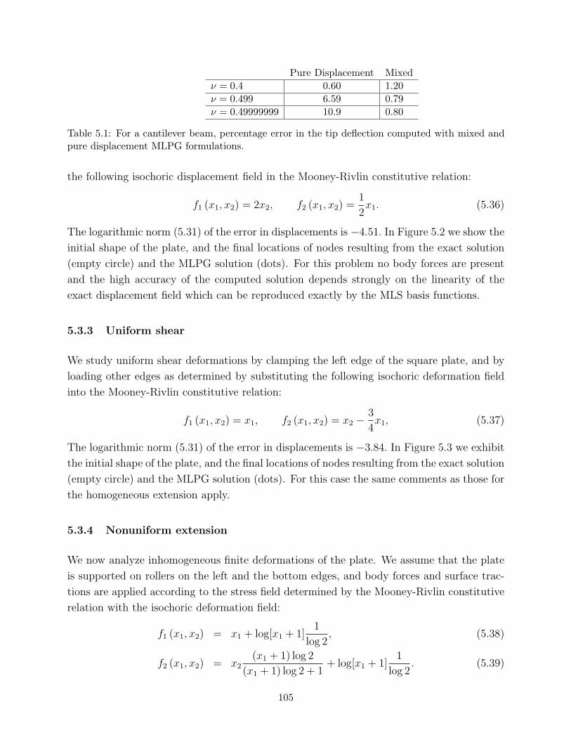
Pure Displacement Mixedν = 0.4 0.60 1.20ν = 0.499 6.59 0.79ν = 0.49999999 10.9 0.80
Table 5.1: For a cantilever beam, percentage error in the tip deflection computed with mixed andpure displacement MLPG formulations.
the following isochoric displacement field in the Mooney-Rivlin constitutive relation:
f1 (x1, x2) = 2x2, f2 (x1, x2) =1
2x1. (5.36)
The logarithmic norm (5.31) of the error in displacements is −4.51. In Figure 5.2 we show the
initial shape of the plate, and the final locations of nodes resulting from the exact solution
(empty circle) and the MLPG solution (dots). For this problem no body forces are present
and the high accuracy of the computed solution depends strongly on the linearity of the
exact displacement field which can be reproduced exactly by the MLS basis functions.
5.3.3 Uniform shear
We study uniform shear deformations by clamping the left edge of the square plate, and by
loading other edges as determined by substituting the following isochoric deformation field
into the Mooney-Rivlin constitutive relation:
f1 (x1, x2) = x1, f2 (x1, x2) = x2 − 3
4x1, (5.37)
The logarithmic norm (5.31) of the error in displacements is −3.84. In Figure 5.3 we exhibit
the initial shape of the plate, and the final locations of nodes resulting from the exact solution
(empty circle) and the MLPG solution (dots). For this case the same comments as those for
the homogeneous extension apply.
5.3.4 Nonuniform extension
We now analyze inhomogeneous finite deformations of the plate. We assume that the plate
is supported on rollers on the left and the bottom edges, and body forces and surface trac-
tions are applied according to the stress field determined by the Mooney-Rivlin constitutive
relation with the isochoric deformation field:
f1 (x1, x2) = x1 + log[x1 + 1]1
log 2, (5.38)
f2 (x1, x2) = x2(x1 + 1) log 2
(x1 + 1) log 2 + 1+ log[x1 + 1]
1
log 2. (5.39)
105

The logarithmic norm (5.31) of the error in computed displacements is −2.78. In Figure 5.4
we evince the initial shape of the plate and the final locations of the nodes resulting from
the exact solution (empty circle) and the MLPG solution (dots).
5.3.5 Nonuniform shear
We assume that the plate is clamped at the left edge, and body forces and surface trac-
tions are applied according to the stress field determined by the Mooney-Rivlin constitutive
relation with deformation field:
f1 (x1, x2) = x1, f2 (x1, x2) = x2 − 1
2(x1)
2, (5.40)
The logarithmic norm (5.31) of the error in displacements computed by the MLPG method
is −2.48. In Figure 5.5 we evince the initial shape of the plate, and the final locations of
nodes resulting from the exact solution (empty circle) and the MLPG solution (dots).
5.3.6 Crack problem
We consider a cracked plate whose geometry is reported in Figure 5.6. By exploiting the
symmetry of the problem, we numerically analyze deformations of the quarter of the domain
depicted in Figure 5.6. In order to accurately analyze effects of the crack, we use secondary
nodes in the neighborhood of the crack tip, all over the domain, and on the boundaries as
shown in Figure 5.7. The secondary nodes located in the neighborhood of the crack tip are
needed for accurately estimating the stress concentration there. The secondary nodes on the
boundaries and in the domain are needed for satisfying well the boundary conditions and
improving the solution inside the domain. From numerical experiments we have observed
that locating only secondary nodes in the neighborhood of the crack tip leads to poor so-
lutions with spurious pressure modes. The total number of nodes used in the simulation is
168.
The plate is loaded with a uniformly distributed dead load of value σ0 = 0.65, and the crack
length equals half of the plate width. In Figure 5.8 we exhibit the deformed shape of the
plate. Recalling that nominal tractions are prescribed on the top surface of the plate, it does
not need to stay horizontal during the deformation process. Also, the total axial force stays
constant even though the width of the plate decreases.
The J-integral in finite elasticity is given by (see, e.g., Legrain, Moes and Verron (2005))
J =
∫
Γ
(Wn1 − n ·Pt ∂wt
∂x1
)dΓ, (5.41)
106

where Γ is the integration contour surrounding the crack tip in the reference configuration,
W is the strain energy density defined by (D.6) in Appendix D, n is the unit outward normal,
and n1 is its component in the crack direction. In order to evaluate J , we use a circular
contour of radius 0.125 centered at the crack tip.
For the linear elastic problem the exact value JL of the J-integral is given by (see, e.g., Kim
and Atluri (2000)):
JL = cπ(1.325)2 1− ν2
Eσ2
0 (5.42)
where 2c is the crack length, being 1 in the present case. In Figure 5.9, we exhibit the J-
integrals computed for the linear and the nonlinear elastic problems. A similar problem has
been studied in Legrain, Moes and Verron (2005) under plane stress conditions, and similar
variations of the J-integral for the linear and the nonlinear problems have been found.
As an additional test of the MLPG mixed formulation, we compute the J-integral for the
linear elastic problem with the pure displacement formulation, and the proposed mixed
pressure-displacement formulation. With the pure displacement formulation the error in the
computed values of J is 71.3%, while when using the mixed formulation the error is only
1.14%.
Figure 5.10 exhibits the crack opening displacements computed using the present MLPG
mixed formulation, and the commercial FE code ANSYS using the 8-node element PLANE183
and 1057 nodes with high concentration at the crack tip. The good agreement between the
two numerical solutions further validates the present mixed formulation. We note that the
proposed MLPG mixed formulation requires only 168 nodes as compared to the 1057 nodes
with the FE method.
Figure 5.11 reports the concentration of the first Piola-Kirchhoff stress, defined as P22/σ0
for different values of the dead tractions. It shows how the mixed formulation enhanced
by secondary nodes is able to capture the stress concentration without leading to spurious
oscillatory behaviors. From Figure 5.11 it can be concluded that increasing the tension in
the plate decreases the order of singularity of the first Piola-Kirchhoff stress at the crack
tip. Figure 5.12 reports instead the concentration of the Cauchy stress, defined as σ22/σ0
for different values of the dead tractions. From Figure 5.12 it can be seen that increasing
the tension in the plate increases the order of singularity of the Cauchy stress at the crack
tip. By comparing plots in Figures 5.11 and 5.12 one evinces that for a nonlinear elastic
problem the orders of singularity in the Cauchy stress and in the first Piola-Kirchhoff stress
are different. Indeed for finite deformation these two tensors are different and they are
related by the deformation gradient.
107
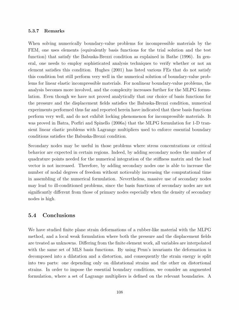
5.3.7 Remarks
When solving numerically boundary-value problems for incompressible materials by the
FEM, one uses elements (equivalently basis functions for the trial solution and the test
function) that satisfy the Babuska-Brezzi condition as explained in Bathe (1996). In gen-
eral, one needs to employ sophisticated analysis techniques to verify whether or not an
element satisfies this condition. Hughes (2001) has listed various FEs that do not satisfy
this condition but still perform very well in the numerical solution of boundary-value prob-
lems for linear elastic incompressible materials. For nonlinear boundary-value problems, the
analysis becomes more involved, and the complexity increases further for the MLPG formu-
lation. Even though we have not proved analytically that our choice of basis functions for
the pressure and the displacement fields satisfies the Babuska-Brezzi condition, numerical
experiments performed thus far and reported herein have indicated that these basis functions
perform very well, and do not exhibit locking phenomenon for incompressible materials. It
was proved in Batra, Porfiri and Spinello (2006a) that the MLPG formulation for 1-D tran-
sient linear elastic problems with Lagrange multipliers used to enforce essential boundary
conditions satisfies the Babuska-Brezzi condition.
Secondary nodes may be useful in those problems where stress concentrations or critical
behavior are expected in certain regions. Indeed, by adding secondary nodes the number of
quadrature points needed for the numerical integration of the stiffness matrix and the load
vector is not increased. Therefore, by adding secondary nodes one is able to increase the
number of nodal degrees of freedom without noticeably increasing the computational time
in assembling of the numerical formulation. Nevertheless, massive use of secondary nodes
may lead to ill-conditioned problems, since the basis functions of secondary nodes are not
significantly different from those of primary nodes especially when the density of secondary
nodes is high.
5.4 Conclusions
We have studied finite plane strain deformations of a rubber-like material with the MLPG
method, and a local weak formulation where both the pressure and the displacement fields
are treated as unknowns. Differing from the finite element work, all variables are interpolated
with the same set of MLS basis functions. By using Penn’s invariants the deformation is
decomposed into a dilatation and a distortion, and consequently the strain energy is split
into two parts: one depending only on dilatational strains and the other on distortional
strains. In order to impose the essential boundary conditions, we consider an augmented
formulation, where a set of Lagrange multipliers is defined on the relevant boundaries. A
108

total Lagrangian formulation is derived and the resulting set of nonlinear algebraic equations
governing finite deformations are solved by Newton-Raphson’s iterations.
A computer code has been developed and used to solve different problems. Computed results
for a body made of a Mooney-Rivlin material under various loading conditions are shown
to compare very well with either analytical solutions or numerical solutions obtained with a
finite element commercial code.
109

x1
x2
Figure 5.1: Geometry and locations of primary nodes for the sample problem studied.
110

Figure 5.2: Uniform extension of a plate: undeformed configuration (shaded), exact solution (emptycircles), MLPG solution (dots).
111

Figure 5.3: Uniform shear of a plate: undeformed configuration (shaded), exact solution (emptycircles), MLPG solution (dots).
112

Figure 5.4: Nonuniform extension of a plate: undeformed configuration (shaded), exact solution(empty circles), MLPG solution (dots).
113

Figure 5.5: Nonuniform shear of a plate: undeformed configuration (shaded), exact solution (emptycircles), MLPG solution (dots).
114

2
1
2
o
(a)
(b)
x1
x1
x2
x2 σ0
Figure 5.6: Geometry of a cracked plate loaded in mode-I.
115

Figure 5.7: Locations of primary (filled circles) and secondary (empty circles) nodes in the quarterof a cracked plate.
116

Figure 5.8: Undeformed (solid line), deformed (dotted) shape of the cracked plate, and final loca-tions of primary (filled circles) and secondary (empty circles) nodes.
117
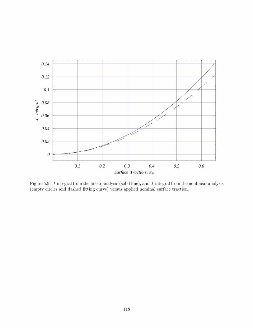
0.1 0.2 0.3 0.4 0.5 0.6Surface Traction , Σ0
0
0.02
0.04
0.06
0.08
0.1
0.12
0.14
J-In
tegr
al
Figure 5.9: J-integral from the linear analysis (solid line), and J-integral from the nonlinear analysis(empty circles and dashed fitting curve) versus applied nominal surface traction.
118

0 0.1 0.2 0.3 0.4 0.5 0.6Surface Traction , Σ0
0
0.02
0.04
0.06
0.08
0.1
CO
D
Figure 5.10: Crack opening displacement computed using the MLPG formulation (diamond), andANSYS FE code (empty circles) versus applied nominal surface traction.
119

0 0.02 0.04 0.06 0.08 0.1 0.12 0.14x2H2cL
1
2
3
4
5
6
7
8P
22Σ
0
Σ0=0.065
Σ0=0.26
Σ0=0.45
Σ0=0.65
Figure 5.11: Normalized first Piola Kirchhoff stress in the neighborhood of the crack tip for differentvalues of the applied nominal surface traction σ0.
0 0.02 0.04 0.06 0.08 0.1 0.12 0.14x2H2cL
2
4
6
8
10
Σ22Σ
0
Σ0=0.065
Σ0=0.26
Σ0=0.45
Σ0=0.65
Figure 5.12: Normalized Cauchy stress in the neighborhood of the crack tip for different values ofthe applied nominal surface traction σ0.
120

Chapter 6
Contributions
We have used the meshless local Bubnov-Galerkin (MLPG6) formulation to analyze free and
forced vibrations of a segmented bar. Three different techniques have been employed to
satisfy the continuity of the axial stress at the interface between two materials: Lagrange
multipliers, jump functions, and modified moving least square basis functions with discontin-
uous derivatives. The essential boundary conditions are satisfied in all cases by the method
of Lagrange multipliers. The related mixed semidiscrete formulations have been shown to be
stable, and optimal in the sense that the ellipticity and the inf-sup (Babuska-Brezzi) condi-
tions are satisfied. Numerical results obtained for a bimaterial bar have been compared with
those from the analytical, and the finite element methods. The monotonic convergence of
first two natural frequencies, first three mode shapes, and a static solution in the L2, and H1
norms has been demonstrated. The relative error in the numerical solution for a transient
problem is also very small.
A consistent one-dimensional distributed electromechanical model of an electrically actu-
ated narrow microbeam with width/height between 0.5 and 2.0 has been derived, and the
pull-in parameters have been extracted with different methods. The model accounts for the
position-dependent electrostatic loading, the fringing field effects due to both the finite width
and the finite thickness of a microbeam, the mid-plane stretching, the mechanical distributed
stiffness, and the residual axial load. Both clamped-clamped, and clamped-free (cantilever)
microbeams are considered. The method of moments has been used to estimate the elec-
trostatic load. The resulting nonlinear fourth-order differential equation under appropriate
boundary conditions has been solved by two methods. Initially, a one-degree-of-freedom
model was proposed to find an approximate solution of the problem. Subsequently, the
meshless local Petrov-Galerkin and the Finite Element methods were used, and results from
the three methods were compared. For the MLPG method the kinematic boundary condi-
tions were enforced by introducing a set of Lagrange multipliers, and the trial and the test
functions are constructed using the generalized moving least squares approximation. The
nonlinear system of algebraic equations arising from the MLPG and the FE methods were
121

solved by using the Displacement Iteration Pull-In Extraction algorithm. Three dimensional
FE simulations of narrow cantilever and clamped-clamped microbeams were also performed
with the commercial code ANSYS. Furthermore, computed results were compared with those
obtained from other distributed models available in the literature, and it was shown that im-
proper fringing fields give over-estimation of the pull-in voltages and inaccurate estimations
of the pull-in deflections.
We have also used the meshless local Bubnov-Galerkin (MLPG6) formulation to analyze
vibrations and transient deformations of a beam with multiple cracks. The trial and the test
functions were constructed using the Generalized Moving Least Squares approximation. The
smoothness of the GMLS basis functions required the use of special techniques to account
for the slope discontinuities at the crack locations. Therefore, a set of Lagrange multipliers
was introduced to model the spring effects at the crack locations and relate motions of the
intact beam segments. The method was applied to study static and transient deformations
of a cracked beam, and to determine its modal properties (frequencies and mode shapes).
Numerical results obtained for a simply supported beam were compared with experimental
findings, analytical predictions, and finite element solutions.
Large deformations of rubber-like materials have also been analyzed by the MLPG method.
A local mixed total Lagrangian weak formulation of non-linear elastic problems was pre-
sented. The deformation gradient was split into deviatoric and dilatational parts. The
strain energy density was written as the sum of two functions: one a function of deviatoric
strain, and the other a function of dilatational strain. The incompressibility or near incom-
pressibility constraint was accounted for by introducing the pressure field, and penalizing
the part of the strain energy density depending upon the dilatational strains. Unlike in
the mixed FE formulation, it was shown that in the MLPG method there is no need for
different sets of basis functions for displacement and pressure fields. Basis functions for
approximating the trial solution and the test functions are generated by the Moving Least
Squares method using the concept of primary and secondary nodes. The formulation does
not require shadow elements or a background mesh, and therefore avoids mesh distortion
difficulties in large deformation problems. Results computed with the MLPG method for a
few sample problems are found to compare very well with either the corresponding analytical
solutions or solutions obtained with a commercial FE code.
122
Bibliography
Abdel-Rahman, E. M., Younis, M. I. and Nayfeh, A. H., “Characterization of the mechani-
cal behavior of an electrically actuated microbeam,” Journal of Micromechanics and Micro-
engeering, Vol. 12, 2002, pp. 759-766.
Andreaus, U., Batra, R. C. and Porfiri, M., “Vibrations of Cracked Euler-Bernoulli Beams
Using Meshless Local Petrov-Galerkin (MLPG) Method,” CMES: Computer Modeling in
Engineering & Sciences, Vol. 9, 2005, pp. 111-132.
Ansys Inc., ANSYS Release 8.0 documentation.
Atluri, S. N. and Zhu, T., “A new Meshless Local Petrov-Galerkin (MLPG) approach in
computational mechanics,” Computational Mechanics, Vol. 22, 1998, pp. 117-127.
Atluri, S. N., Cho, J. Y. and Kim, H.-G., “Analysis of Thin Beams, Using the Meshless Local
Petrov-Galerkin Method, with Generalized Moving Least Squares Interpolations,” Compu-
tational Mechanics, Vol. 24, 1999, pp. 334-347.
Atluri, S. N. and Shen, S. P., The Meshless Local Petrov-Galerkin (MPLG) Method, Tech.
Science Press, California, 2002.
Atluri, S. N. and Shen, S., “The Meshless Local Petrov-Galrkin (MLPG) Method: A Sim-
ple & Less-costly Alternative to Finite Element and Boundary Element Methods,” CMES:
Computer Modeling in Engineering & Sciences, Vol. 3, 2004, pp. 11-51.
Atluri, S. N., Han, Z. D. and Rajendran, A. M., “A new implementation of the meshless
finite volume method, through the MLPG “Mixed” approach,” CMES: Computer Modeling
in Engineering & Sciences, Vol. 6, 2004, pp. 491-513.
Barke, E., “Line-to-Ground Capacitance Calculation for VLSI: A Comparison,” IEEE Trans-
actions on Computer-Aided Design, Vol. 7, 1988, pp. 295-298.
Bathe, K. J., Finite Element Procedures, Prentice-Hall, Englewood Cliffs, New Jersey, 1996.
Batra, R. C., “Finite plane strain deformation of rubberlike materials,”. International Jour-
nal for Numerical Methods in Engineering, Vol. 15, 1980, pp. 145-160.
123

Batra, R. C. and Ching H.-K., “Analysis of Elastodynamic Deformations near a Crack/Notch
Tip by the Meshless Local Petrov-Galerkin (MLPG) Method,” CMES: Computer Modeling
in Engineering & Sciences, Vol. 3, 2002, pp. 717-730.
Batra, R. C. and Liang, X.-Q., “Finite Dynamic Deformations of Smart Structures,” Com-
putational Mechanicas, Vol. 20, 1997, pp. 427-438.
Batra, R., Porfiri, M. and Spinello, D., “Treatment of Material Discontinuity in Two Meshless
Local Petrov-Galerkin (MLPG) Formulations of Axisymmetric Transient Heat Conduction,”
International Journal for Numerical Methods in Engineering, Vol. 61, 2004, pp. 2461-2479.
Batra, R. C., Porfiri, M. and Spinello, D., “Free and Forced Vibrations of a Segmented
Bar by a Meshless Local Petrov-Galerkin (MLPG) Formulation,” Computational Mechanics,
DOI 10.1007/s00466-006-0049-6, 2006a, (available online).
Batra, R. C., Porfiri,M. and Spinello, D., “Electromechanical Model of Electrically Actuated
Narrow Microbeams,” Journal of MicroElectroMechanical Systems, 2006b, (accepted).
Batra, R. C., Porfiri,M. and Spinello, D., “Analysis of Electrostatic MEMS using Meshless
Local Petrov-Galerkin (MLPG) method,” Journal of Engineering Analysis with Boundary
Elements, 2006c, (accepted).
Batra, R. C. and Vidoli, S., “Higher Order Piezoelectric Plate Theory Derived from a Three-
Dimensional Variational Principle,” AIAA Journal, Vol. 40, 2002, pp. 91-104.
Batra, R. C. and Wright, T. W., “Steady State Penetration of Rigid Perfectly Plastic Tar-
gets,” International Journal of Engineering Science, Vol. 24, 1986, pp. 41-54.
Belytschko, T., Lu, Y. Y. and Gu, L., “Element-free Galerkin Methods,” International
Journal for Numerical Methods in Engineering, Vol. 37, 1994, pp. 229-256.
Charrier, P., Dacorogna, B., Hanouzet, B. and Laborde, P., “An existence theorem for
sligthly incompressible materials in non linear elasticity,” SIAM Journal on Mathematical
Analysis Vol. 19, 1988, pp. 70-85.
Chen, J. S., Pan, C. and Chang, T. Y. P., “On the control of pressure oscillations in bilinear-
displacements costant-pressure elements,” Computer Methods in Applied Mechanics and En-
gineering, Vol. 128, 1995, pp. 137-152.
Chen, J. S., Pan, C. and Wu, C. T., “Large deformation of rubber based on a reproducing
kernel particle method,” Computational Mechanics, Vol. 19, 1997, pp. 211-227.
Chen, J. S., Han, W., Tu, C. T. and Duan, W., “On the perturbed Lagrangian for nearly
incompressible and incompressible hyperelasticity,” Computer Methods in Applied Mechanics
and Engineering, Vol. 142, 1997, pp. 335-351.
124

Ching H.-K. and Batra, R. C., “Determination of Crack Tip Fields in Linear Elastostatics
by the Meshless Local Petrov-Galerkin (MLPG) Method,” CMES: Computer Modeling in
Engineering & Sciences, Vol. 2, 2001, pp. 273-289.
Chondros, T. G., “The continuous crack flexibility model for crack identification,” Fatigue
& Fracture of Engineering Materials & Structures, Vol. 24, 2001, pp. 643-650.
Chondros, T. G., Dimarogonas, A. D. and Yao, J., “A continuous cracked beam vibration
theory,” Journal of Sound and Vibration, Vol. 215, 1998, pp. 17-34.
Chondros, T. G. and Dimarogonas, A. D., “Vibration of a beam with a breathing crack,”
Journal of Sound and Vibration, Vol. 239, 2001, pp. 57-67.
Christides, S. and Barr, A. D. S., “One-dimensional theory of cracked Bernoulli-Euler
beams,” International Journal of Mechanical Sciences, Vol. 26, 1984, pp. 639-648.
Crisfield, M. A., Non-linear Finite Element Analysis of Solids and Structures Vol 2, Advanced
Topics, Wiley, Chichester, 1998.
Collins, E. R., Foundations for Microwave Engineering 2nd Edition, McGraw-Hill, New York,
1992, pp. 130-153.
Cordes, L. W. and Moran, B., “Treatment of Material Discontinuity in the Element-Free
Galerkin Method,” Computer Methods in Applied Mechanics and Engineering, Vol. 139,
1996, pp. 75-89.
Carneiro, S. H. S. and Inman, D. J., “Continuous model for the transverse vibration of
cracked Timoshenko beams,” Transactions of the ASME, Vol. 124, 2002, pp. 310-320.
Coventor Inc., “Pull-in Voltage Analysis of Electrostatically-Actuated Beams Verifying Ac-
curacy of Coventor Behavioral Models”, available online at www.coventor.com.
Degani-Bochobza, O., Elata, D. and Nemirovsky, Y., “An Efficient DIPIE Algorithm for
CAD of Electrostatically Actuated MEMS devices,” Journal of Microelectromechanical Sys-
tems, Vol. 11, 2002, pp. 612-620.
Dimarogonas, A. D., “Vibration of cracked structures: A state of the art review,” Engineering
Fracture Mechanics, Vol. 55, 1996, pp. 831-857.
Duarte, C. A. M. and Oden, J. T., “Hp clouds—an hp Meshless Method,” Numerical Methods
for Partial Differential Equations, Vol. 12, 1996, pp. 673-705.
Ferreira, A. J. M., Batra, R. C., Roque, C. M. C., Qian L. F. and Martins, P. A. L. S., “Static
Analysis of Functionally Graded Plates Using Third-order Shear Deformation Theory and a
Meshless Method,” Composite Structures, Vol. 69, 2005, pp. 449-457.
125

Gabbay, L. D., Mehner, J. E. and Senturia, S. D., “Computer-aided generation of nonlin-
ear reduced-order dynamic macromodels I: Non-stress-stiffened case,” Journal of Microelec-
tromechanical Systems, Vol. 9, 2000, pp. 262-269.
Gadala, M. S., “Numerical solution of non-linear problems of continua-I, Survey of incom-
pressibility constraints and software aspects,” Computers and Structures, Vol. 22, 1986, pp.
841-855.
Gounaris, G. and Dimarogonas, A., “A finite element of a cracked prismatic beam for struc-
tural analysis,” Computers & Structures, Vol. 28, 1988, pp. 309-313.
Gounaris, G., Papadoupolos C. A. and Dimarogonas, A., “Crack Identification in beams by
coupled response measurements. Computers & Structures, Vol. 58, 1996, pp. 299-305.
Gudmunson, P., “The dynamic behaviour of slender structures with cross-sectional cracks,”
Journal of the Mechanics and Physics of Solids, Vol. 31, 1983, pp. 329-345.
Gu, Y. T. and Liu, G. R., “A Meshless Local Petrov-Galerkin (MLPG) Method for Free
and Forced Vibration Analyses for Solids,” Computational Mechanics, Vol. 27, 2001a, pp.
188-198.
Gu, Y. T. and Liu, G. R., “A meshless local Petrov–Galerkin (MLPG) formulation for static
and free vibration analysis of thin plates,” Computer Modeling in Engineering & Sciences,
Vol. 2, 2001b, pp. 463-476.
Harrington, R. F., Field Computation by Moment Methods. Piscataway, NJ: IEEE Press,
1993, pp. 229.
Hermann, L. R., “Elasticity equations for incompressible and nearly incompressible materials
by variational theorem,” AIAA Journal, Vol. 3, 1965, pp. 1896-1900.
Hughes, T. J. R., The Finite Element Method. Linear Static and Dynamic Finite Element
Analysis, Prentice-Hall, New Jersey, 2001.
Hung, E. S. and Senturia, S. D., “Extending the Travel Range of Analog-Tuned Electrostatic
actuators,” Journal of Microelectromechanical Systems, Vol. 8, 1999, pp. 497-505.
Iesan, D., Saint-Venant’s problem, Springer-Verlag, New York, 1987.
Kansa, E. J., “Multiquadrics-A Scattered Data Approximation Scheme with Applications to
Computational Fluid Dynamics, ii: Solutions to Parabolic, Hyperbolic and Elliptic Partial
Differential Equations,” Computer & Mathematics with Applications, Vol. 19, 1990, pp.
147-161.
Khiem, N. T., Lien, T. V., “Multi-crack detection for beam by the natural frequencies,”
Journal of Sound and Vibration, Vol. 1-2, 2004, pp. 175-184.
126

Kim, H.-G. and Atluri, S. N., “Arbitrary Placement of Secondary Nodes, and Error Control,
in the Meshless Local Petrov-Galerkin (MLPG) Method,” CMES: Computer Modeling in
Engineering & Sciences, Vol. 1, 2000, pp. 11-32.
Krongauz, Y. and Belytschko, T., “EFG Approximation with Discontinuous Derivatives,”
International Journal for Numerical Methods in Engineering, Vol. 41, 1998, pp. 1215-1233.
Kuang, J.-H. and Chen, C.-J., “Dynamic characteristics of shaped micro-actuators solved
using the differential quadrature method,” Journal of Micromechanics and Microengeering,
Vol. 14, 2004, pp. 647-655.
Lancaster, P. and Salkauskas, K., “Surfaces Generated by Moving Least Squares Methods,”
Mathematics of Computation, Vol. 37, 1981, pp. 141-158.
Landau, L. D. and Lifshitz, E. M., Theory of elasticity, New York, Pergamon Press, 1986.
Legrain, G., Moes, N. and Verron, E., “Stress analysis around crack tips in finite strain
problems using the eXtended finite element method,” International Journal for Numerical
Methods in Engineering, Vol. 63, 2005, pp. 290-314.
Liu, G. R., Mesh Free Methods, CRC Press, Boca Raton, Florida, 2003.
Liu, W. K., Jun, S., Adee, J. and Belytschko, T., “Reproducing Kernel Particle Methods
for Structural Dynamics,” International Journal for Numerical Methods in Engineering, Vol.
38, 1995, pp. 1655-1679.
Liu, W., Jun, S. and Zhang, Y., “Reproducing kernel particle method,” International Journal
for Numerical Methods in Fluids, Vol. 20, 1995, pp. 1081-1106.
Lucy, L. B., “A Numerical Approach to the Testing of the Fission Hypothesis,” The Astro-
nomical Journal, Vol. 82, 1977, pp. 1013-1024.
Luzzato, E., “Approximate computation of non-linear effects in a vibrating cracked beam,”
Journal of Sound and Vibration, Vol. 265, 2003, pp. 745-763.
Mahmoud, M. A., Zaid, M. A. and Al Harashani, S., “Numerical frequency analysis on uni-
form beams with a transverse crack,” Communications in Numerical Methods in Engineering,
Vol. 15, 1999, pp. 709-715.
Mackerle, L., “Rubber and rubber-like materials, finite-element analyses and simulations, an
addendum: a bibliography (1997-2003),” Modelling and Simulation in Materials Science and
Engineering, Vol. 12, 2004, pp. 1031-1053.
Meijs, N. V. D. and Fokkema, J. T., “VLSI circuit reconstruction from mask topology,”
Integration, Vol. 2, 1984, pp. 85-119.
127

Meirovitch, L., Fundamentals of Vibrations, McGraw Hill, New York, 2001.
Melenk, J. M. and Babuska, I., “The Partition of Unity Finite Element Method: Basic
Theory and Applications,” Computer Methods in Applied Mechanics and Engineering, Vol.
139, 1996, pp. 289-314.
Mura, T. and Koya, T., Variational methods in mechanics, Oxford University Press, New
York, 1992.
Nagdi, K., Rubber as an Engineering Material: Guidelines for Users, Hanser, New York,
1993.
Nathanson, H. C., Newell, W. E., Wickstrom, R. A. and Davis, J. R, “The Resonant Gate
Transistor,” IEEE transactions on Electron Devices Vol. 14, 1977, pp. 117-133.
Nayroles, B., Touzot, G. and Villon, P., “Generalizing the Finite Element Method: Diffuse
Approximation and Diffuse Elements,” Computational Mechanics, Vol. 10, 1992, pp. 307-
318.
Nguyen, C. T. C., Katehi, L. P. B. and Rebeiz, G. M., “Micromachined devices for wireles
communications,” Proceedings IEEE, Vol. 86, 1998, pp. 1756-1768.
Noguchi, H. and Sachiko, M., “Analysis of Structure with Material Interface by Meshfree
Method,” CMES: Computer Modeling in Engineering & Sciences, 2006, (to appear).
Ogden, R. W., Nonlinear Elasticity with Application to Material Modeling. Lecture notes 6
in IPPTPAN, Warsaw, 2004.
Osterberg, P. M. and Senturia, S. D., “M-TEST: A test chip for MEMS material property
measurement using electrostatically actuated test structures,” Journal of Microelectrome-
chanical Systems, Vol. 6, 1997, pp. 107-118.
Ostachowicz, W. M. and Krawczuk, M., “Analysis of the effect of cracks on the natural
frequencies of a cantilever beam,” Journal of Sound and Vibration, Vol. 150, 1991, pp.
191-201.
Palmer, H. B., “Capacitance of a parallel-plate capacitor by the Schwartz-Christoffel trans-
formation,” Transactions AIEE, Vol. 56, 1927, p. 363.
Pamidighantam, S., Puers, R., Baert, K. and Tilmans, H. A. C., “Pull-in voltage analysis
of electrostatically actuated beam structures with fixed-fixed and fixed-free end conditions,”
Journal of Micromechanics and Microengeering, Vol. 12, 2002, pp. 458-464.
Peng, S. H. and Chang, W., “A compressible approach in finite element analysis of rubber-
elastic materials,” Computers and Structures, Vol. 62, 1997, pp. 573-593.
128

Penn, R.-W., “Volume changes accompanying the extension of rubber,” Journal of Rheology,
Vol. 4, 1970, pp. 509-517.
Press, W. H., Flannery, B. P., Teukolsky, S. H. and Vetterling, W. T., Numerical Recipes,
Cambridge University Press, New York, 1989.
Pugno, N., Surace, C. and Ruotolo, R., “Evaluation of the non-linear dynamic response
to harmonic excitation of a beam with several breathing cracks,” Journal of Sound and
Vibration, Vol. 235, 2000, pp. 749-762.
Qian, L. F. and Batra, R. C., “Transient Thermoelastic Deformations of a Thick Functionally
Graded Plate,” Journal of Thermal Stresses, Vol. 27, 2004, pp. 705-740.
Qian, L. F. and Batra, R. C., “Design of Bidirectional Functionally Graded Plate for Optimal
Natural Frequencies,” Journal of Sound and Vibration, Vol. 280, 2005, pp. 415-424.
Qian, L. F., Batra, R. C. and Chen, L. M., “Elastostatic Deformations of a Thick Plate by
Using Higher-order Shear and Normal Deformable Plate Theory and Two Meshless Local
Petrov-Galerkin (MLPG) Methods,” CMES: Computer Modeling in Engineering & Sciences,
Vol. 4, 2003a, pp. 161-176.
Qian, L. F., Batra, R. C. and Chen, L. M., “Free and Forced Vibrations of Thick Rectangular
Plates by Using Higher-order Shear and Normal Deformable Plate Theory and Meshless Local
Petrov-Galerkin (MLPG) Method,” CMES: Computer Modeling in Engineering & Sciences,
Vol. 4, 2003b, pp. 519-534.
Qian, L. F., Batra, R. C. and Chen, L. M., “Analysis of Cylindrical Bending Thermoelastic
Deformations of Functionally Graded Plates by a Meshless Local Petrov-Galerkin Method,”
Computational Mechanics, Vol. 33, 2004a, pp. 263-273.
Qian, L. F., Batra, R. C. and Chen, L. M., “Static and Dynamic Deformations of a Thick
Functionally Graded Elastic Plate by Using a Higher-Order Shear and Normal Deformable
Plate Theory and Meshless Local Petrov-Galerkin (MLPG) Method,” Composites: Part B,
Vol. 35, 2004b, pp. 685-697.
Qian, G. L., Gu, S.-N. and Jiang, J.-S., “The dynamic behaviour and crack detection of a
beam with a crack,” Journal of Sound and Vibration, Vol. 138, 1990, pp. 233-243.
Raju, I. S. and Phillips, D. R., “Further developments in the MLPG Method for Beam
Problems,” CMES: Computer Modeling in Engineering & Sciences, Vol. 4, 2003, pp. 141-
159.
Rivlin, R. S., “Large Elastic deformations of isotropic materials IV, furher developments
of general theory,” Philosophical Transactions of the Royal Society of London A, 1948, pp.
129

379-397.
Rizos, P. F., Aspragathos, N. and Dimarogonas, A. D., “Identification of crack location and
magnitude in a cantilever beam from the vibration mode,” Journal of Sound and Vibration,
Vol. 138, 1988, pp. 381-388.
Ruotolo, R., Surace, C., Crespo, P. and Storer, D., “Harmonic analysis of the vibrations
of a cantilevered beam with a closing crack,” Computers & Structures, Vol. 61, 1996, pp.
1057-1074.
Scharnost, T. and Pian, T. H. H., “Finite element analysis of rubber-like materials by a
mixed model,” International Journal for Numerical Methods in Engineering, Vol. 12, 1978,
pp. 665-676.
Saccomandi, G., Universal results in finite elasticity. Non-Linear Elasticity, (edited by Y.
Fu and R. Ogden) Cambridge University Press, Cambridge, 2001.
Senturia, S. D., Harris, R. M., Johnson, B. P., Kim, S., Nabors, K., Shulman, M. A. and
White, J. K., “A computer-aided design system for microelectromechanical systems (MEM-
CAD),” Journal of Microelectromechanical Systems, Vol. 1, 1992, pp. 3-13.
Shapoorabadi, R. J. and Kirk, A. G., “Comparison of three finite element models for analysis
of MEMS micromirrors,” Proceedings SPIE, International Conference on Applications of
Photonic Technology, Photonics North, Vol. 5577, 2004, pp.849-859.
Shen, M.-H. H. and Chu, Y. C., “Vibrations of a beam with a fatigue crack,” Computers &
Structures, Vol. 45, 1992, pp. 79-93.
Shen, M.-H. H. and Pierre C., “Natural modes of Bernoulli-Euler beams with symmetric
cracks,” Journal of Sound and Vibration, Vol. 138, 1990, pp. 115-134.
Shen, M.-H. H. and Pierre, C., “Free vibrations of beams with single-edge crack,” Journal
of Sound and Vibration, Vol. 170, 1994, pp. 237-259.
Simo, J. C. and Hughes, J. R. T., Computational Inelasticity, Springer, NewYork, 1998.
Sukumar, N., Moran, B. and Belytschko, T., “The Natural Element Method in Solid Me-
chanics,” International Journal for Numerical Methods in Engineering, Vol. 43, 1998, pp.
839-887.
Sundermeyer, J. M. and Weaver, R. L., “On crack identification and characterization in a
beam by non-linear vibration analysis,” Journal of Sound and Vibration, Vol. 183, 1995, pp.
857-871.
Taylor, G. I., “The Coalescence of Closely Spaced drops when they are at different electric
potentials,” Proceedings of the Royal Society A, Vol. 306, 1968, pp. 423-434.
130
Tilmans, H. A. and Legtenberg, R., “Electrostically driven vacuum-encapsulated polysilicon
resonators: Part II. Theory and Performance,” Sensors and Actuators A, Vol. 45, 1994, pp.
67-84.
Timoshenko, S. P. and Goodier, J. N., Theory of Elasticity, 3rd edition. Mc Graw Hill, New
York, 1970.
Vidoli, S. and Batra, R. C., “Derivation of Plate and Rod Equations for a Piezoelectric Body
from a Three-Dimensional Variational Principle,” Journal of Elasticity, Vol. 59, 2000, pp.
23-50.
Warlock, A., Ching, H.-K., Kapila, A. K. and Batra, R. C. “Plane Strain Deformations of
an Elastic Material Compressed in a Rough Rectangular Cavity,” International Journal of
Engineering Science, Vol. 40, 2002, pp. 991-1010.
Wendland, H., “Piecewise Polynomial, Positive Definite and Compactly Supported Radial
Basis Functions of Minimal Degree,” Advances in Computational Mathematics, Vol. 4, 1995,
pp. 389-396.
Younis, M. .I, Abdel-Rahman, E. M. and Nayfeh, A. H., “A Reduced-Order Model for Elec-
trically Actuated Microbeam-Based MEMS,” Journal of Microelectromechanical Systems,
Vol. 12, 2003, 6pp. 72-680.
Zhang, G. M. and Batra, R. C., “Modified Smoothed Particle Hydrodynamics Method and its
Application to Transient Problems,” Computational Mechanics, Vol. 34, 2004, pp. 137-146.
131

Appendix A
MLS and GMLS approximations
A.1 Moving Least Squares (MLS) basis functions
The MLS approximation, proposed by Lancaster and Salkauskas (1981), allows for an accu-
rate reconstruction of a given trial function on the entire domain, from the knowledge of its
values at some, suitably chosen, scattered points.
Consider a continuous scalar function q defined on the d-dimensional connected domain Ω.
The generic point in Ω is indicated by x and its coordinates in a rectangular Cartesian
coordinate system are x1, x2, . . . , xd. The (fictitious) nodal values at N scattered points
N = x1,x2, ...,xN in Ω are collected into the N -vector q = [q1, ..., qN ]T. The global
approximation qh of q in Ω is defined as
q (x) ' qh (x) = pT (x) a (x) , x ∈ Ω, (A.1)
where
pT (x) = [p1 (x) , p2 (x) , ..., pm (x)] , (A.2)
is a monomial basis. For example in the two-dimensional problem a complete monomial
basis of order 2 ispT (x) = [1, x1, x2] , linear basis, m = 3. (A.3)
The m-vector a (x) = [a1 (x) , · · · , am (x)]T is composed of indeterminate coefficients, which
vary with the point x in the domain Ω. At each location x in Ω these coefficients are
determined by a local least square approximation of q (x) on a small neighborhood Ωx of x.
The local approximation qx (x) is defined by
q (x) ' qx (x) = pT (x) a (x) , x ∈ Ωx ⊂ Ω. (A.4)
Therefore, in a small neighborhood of a generic point x the coefficients ai are treated as
the unknown constants of the classical polynomial least square approximation, and they are
132

determined by minimizing the following functional Jx representing the weighted discrete L2
error norm
Jx (a) =N∑
i=1
Wi (x) [qx (xi)− qi]2 . (A.5)
The function Wi is the weight function of node i.
At a given location x only few terms in the summation (A.5) are not zero since the supports
of the weight functions Wi are much smaller than the domain Ω. This reduces the memory
allocations when implementing the algorithm in a computer code, and strengthens the local
character of the MLS approximation.
The functional Jx may be rewritten in matrix notation as
Jx (a) = (Pa− q)T W (x) ( Pa− q) , (A.6)
where P is a (N, m) matrix of real numbers:
PT =[
pT (x1) ... pT (xN)], (A.7)
and W is the following (N, N) diagonal matrix
W (x) = Diag[
W1 (x) ... WN (x)]. (A.8)
The stationarity of Jx with respect to a yields:
A (x) a (x) = B (x) q, (A.9)
where the (m,m) and the (m,N) matrices A and B are defined by
A (x) = PTW (x)P, B (x) = PTW (x) . (A.10)
We note that the matrices A and B depend on the spatial coordinate x only through the
weight functions, since P is a matrix of real numbers. Solving for a in (A.9) and substituting
the result in the global approximation (A.4) we get the MLS approximation
qh (x) = pT (x)A−1 (x)B (x) q, (A.11)
which, upon introducing the basis functions ψ (x) , can be expressed as
qh (x) = ψT (x) q, ψ =[
ψ1 ... ψN
]T, ψT (x) = pT (x)A−1 (x)B (x) . (A.12)
For node xi,
qh (xi) 6= qi. (A.13)
133

That is, the value of the approximating function at a node does not equal, in general, the
value at that node of the function. Said differently, ψj (xi) 6= δij, where δij is the Kronecker
delta.
The MLS expansion (A.12) is well defined only if the matrix A in (A.10) is non-singular. It
can be seen that this is the case if and only if the rank of the n ×m matrix Px, obtained
from P by deleting rows corresponding to those nodes whose weight function vanishes at x,
equals m. Obviously, a necessary condition for a well-defined MLS approximation is that at
least m nodal weight functions do not vanish at x. However, this condition is not sufficient
(see, e.g., Atluri, Cho and Kim (1999)).
The smoothness of the MLS trial functions is completely determined by the smoothness of
the weight functions, since the polynomial basis is infinitely differentiable. If α indicates the
minimum order of differentiability of all weight functions, then from (A.10) it is evident that
the trial functions are at least α times differentiable.
In the analysis, the computation of the derivative of the MLS basis functions in (A.12) is
needed. To save computational effort, it is advisable to compute explicitly the first derivative
of the inverse of the matrix A with respect to the coordinate xj from the identity:
AA−1 = 1; (A.14)
hence∂ (A−1)
∂xj
= −A−1 ∂A
∂xj
A−1, (A.15)
where j = 1, . . . , d. Therefore, only the knowledge of the weight functions, and their deriva-
tive is needed to compute the derivative of A−1.
In the literature (see, e.g., Atluri and Shen (2002)), fourth-order spline and Gauss weight
functions are widely used. For one dimensional problems as those analyzed in Chapter 2, we
employ the fourth-order spline weight function:
Wi (x) =
1− 6
(di
ri
)2
+ 8
(di
ri
)3
− 3
(di
ri
)4
, di ≤ ri
0, di > ri
, (A.16)
where di = |x−xi| is the distance from node xi to point x on the one dimensional domain,
and ri is the radius of support of the weight function Wi. For two dimensional domains we
use Gaussian weight functions with square supports:
Wi (x) =
exp
−
x1−xi1ci
2k−exp
−
rici
2k
1−exp
−
rici
2k exp
−
x2−xi2ci
2k−exp
−
rici
2k
1−exp
−
rici
2k ,
0 ≤ |x1 − xi1| , |x2 − xi2| ≤ ri
0, |x1 − xi1| , |x2 − xi2| > ri
(A.17)
134

where ci and k are constants controlling the shape of the weight function, and ri is the length
of the side of the square support.
The numerical integration of the MLS basis functions for two or three-dimensional prob-
lems may be computationally time-consuming due to the large number of quadrature points
required. Therefore, when a large number of nodes is needed in the formulation, it is advis-
able to make use of the so-called secondary nodes. These nodes provide additional degrees
of freedom without significantly increasing the number of required quadrature points. The
approach that we suggest for adding secondary nodes in the formulation is similar to that
presented in Kim and Atluri (2000) with the main difference being that we do not require
a background mesh. We use the traditional MLS approximation for the generation of the
entire set of trial functions, whereas in Kim and Atluri (2000) the finite element basis func-
tions are used as weight functions for the primary nodes. We partition the set of nodes into
two subsets: the set of primary nodes NP and the set of secondary nodes NS.
Each secondary node xi ∈ NS is associated to its closest primary node ı, xı ∈ NP , and
its weight function is the product of the weight function of the primary one, Wı(x), and
an auxiliary weight function Wı(x). In this way, the support of the weight function of a
secondary node is included in the support of the weight function of the corresponding primary
node. The number of quadrature points used in the numerical evaluation of matrices and
vectors in the discrete formulation (5.30) is only dictated by the number of primary nodes
and by supports of their weight functions. Hence integrals in (5.30) can be computed by
adding integrals on the partitions of the domain generated by intersecting supports of weight
functions of the primary nodes.
For two-dimensional problems we use
Wi (x) =
(1− 6
(x1−xi1
ri
)2
+ 8(
x1−xi1
ri
)3
− 3(
x1−xi1
ri
)4)×
(1− 6
(x2−xi2
ri
)2
+ 8(
x2−xi2
ri
)3
− 3(
x2−xi2
ri
)4)
,
0 ≤ |x1 − xi1| , |x2 − xi2| ≤ ri
0, |x1 − xi1| , |x2 − xi2| > ri
(A.18)
where ri is a constant controlling the support of the weight function.
A.2 Generalized Moving Least Squares (GMLS) basis functions
The generalized moving least squares approximation (GMLS) proposed by Atluri, Cho and
Kim (1999) generalizes that proposed in Lancaster and Salkauskas (1981) by allowing for the
accurate reconstruction of a given trial function on the entire domain, from the knowledge
135

of its values and of its first derivatives at some, suitably chosen, scattered points.
Consider the function w having continuous first derivative on the domain Ω. The (fictitious)
nodal values and (fictitious) derivatives at the scattered points N = x1, x2, ..., xN in Ω are
collected into the two N -vectors w = [w1, ..., wN ]T and ϑ =[ϑ1, ..., ϑN
]T
respectively, where
the superscript T indicates transposition. The global approximation wh on Ω is defined as
w (x) ' wh (x) = pT (x) a (x) , x ∈ Ω, (A.19)
where
pT (x) =[1, x, x2, ..., xm−1
](A.20)
is a complete monomial basis of degree m− 1.
The m-vector a (x) = [a1 (x) , ..., am (x)]T is composed of indeterminate coefficients, which
vary with the abscissa x on the domain Ω. At each location x on Ω these coefficients are
determined by a local least square approximation of w (x) on a small neighborhood Ωx of x.
The local approximation wx (x) is defined by
w (x) ' wx (x) = pT (x) a (x) , x ∈ Ωx ⊂ Ω. (A.21)
In a small neighborhood of a generic point x the coefficients ai are treated as the unknown
constants of a classical polynomial least square approximation. Therefore, they are deter-
mined by minimizing the functional Jx representing the weighted discrete H1 error norm
(see, e.g., Atluri, Cho and Kim (1999); Figure A.1 shows the GMLS approximation), and
defined by
Jx (a) =N∑
i=1
W(w)i (x) [wx (xi)− wi]
2 +N∑
i=1
W(ϑ)i (x)
[w′
x (xi)− ϑi
]2
, (A.22)
where the superimposed prime indicates derivative with respect to the x coordinate. Func-
tions W(w)i and W
(ϑ)i are weight functions of node i and are characterized by the following
properties: (i) they are continuous, (ii) they equal one at x = xi, (iii) they vanish when
x /∈(xi −R
(w)i , xi + R
(w)i
)and x /∈
(xi −R
(ϑ)i , xi + R
(ϑ)i
), respectively, and are positive
elsewhere. The parameters R(w)i and R
(ϑ)i measure semi-supports of the weight functions
W(w)i and W
(ϑ)i respectively.
136

At a given location x only a few terms in summation (A.22) do not vanish since the supports
R(w)i and R
(ϑ)i of the weight functions W
(w)i and W
(ϑ)i are much smaller than the size of
Ω. This is used to reduce the memory allocations when implementing the algorithm in a
computer code. Lower bounds of R(w)i and R
(ϑ)i are stated in Atluri, Cho and Kim (1999)
for assuring the regularity of the GMLS basis functions.
The stationarity of Jx with respect of a yields
A (x) a (x) = B (x)
[w
ϑ
], (A.23)
where the (m,m) and the (m,N) matrices A and B are defined by
A (x) = PTW(w) (x)P+ (P′)TW(ϑ) (x)P′, B (x) =
[PTW(w) (x) (P′)T W(ϑ) (x)
].
(A.24)
Here W(w) and W(ϑ) are (N,N) diagonal matrices defined by
W(w) (x) = Diag[
W(w)1 (x) ... W
(w)N (x)
], W(ϑ) (x) = Diag
[W
(ϑ)1 (x) ... W
(ϑ)N (x)
],
(A.25)
and P, P′ are (N, m) matrices of real numbers defined by
PT =[
p (x1) ... p (xN)], (P′)T
=[
p′ (x1) ... p′ (xN)]. (A.26)
Solving (A.23) for a (x) and substituting for a (x) in the global approximation (A.21) we
obtain the GMLS approximation
wh (x, t) = ψ(w) (x)T w + ψ(ϑ) (x)T ϑ, (A.27)
where the vectors of basis functions ψ(w) (x) and ψ(ϑ) (x) are given by
ψ(w) = p (x)T A−1 (x)PTW(w) (x) , ψ(ϑ) = pT (x)A−1 (x) (P′)TW(ϑ) (x) . (A.28)
It is convenient to group the nodal variables and the GMLS basis functions in the 2N -vectors
s and ψ, respectively.
The smoothness of the GMLS trial functions is completely determined by the smoothness of
the weight functions, since the monomial basis is infinitely differentiable. If α− 1 indicates
137
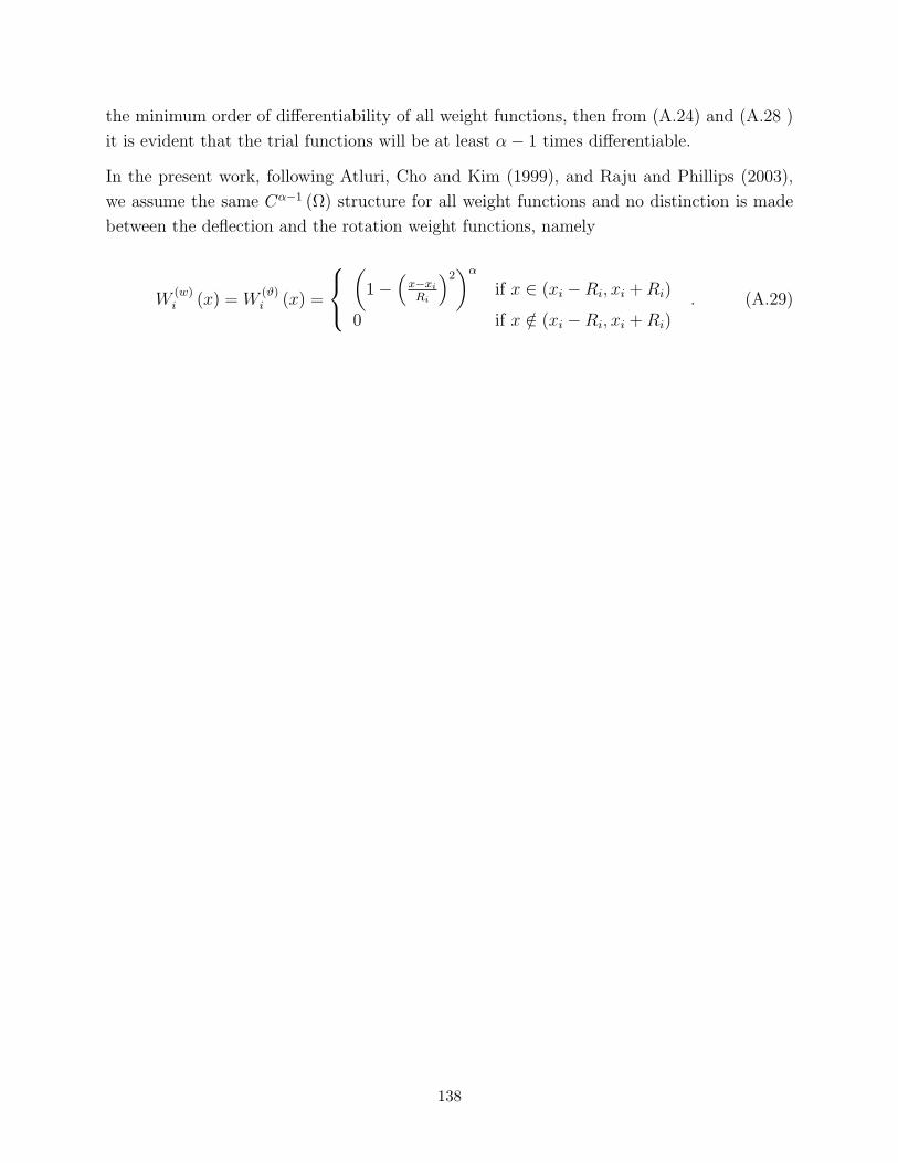
the minimum order of differentiability of all weight functions, then from (A.24) and (A.28 )
it is evident that the trial functions will be at least α− 1 times differentiable.
In the present work, following Atluri, Cho and Kim (1999), and Raju and Phillips (2003),
we assume the same Cα−1 (Ω) structure for all weight functions and no distinction is made
between the deflection and the rotation weight functions, namely
W(w)i (x) = W
(ϑ)i (x) =
(1−
(x−xi
Ri
)2)α
if x ∈ (xi −Ri, xi + Ri)
0 if x /∈ (xi −Ri, xi + Ri). (A.29)
138

wxx = pTxax
x xx i
wi
ϑ i
Figure A.1: Sketch of the GMLS approximation.
139

Appendix B
Closed-form expressions for free andforced vibrations of the segmentedbar in Chapter 2
B.1 Free vibrations
We consider in eqs. (2.10) and (2.11) displacement fields of the form
w1 (x, t) = W1 (x) exp (iωt) , w2 (x, t) = W2 (x) exp (iωt) . (B.1)
Imposing homogeneous form of boundary conditions (2.12), (2.13), (2.14), and (2.15) in
(2.10), (2.11), we obtain the following trascendental characteristic equation for the frequency
ω:
tan
(a
c1
ω
)tan
(L− a
c2
ω
)=
c1E2
c2E1
. (B.2)
The corresponding mode shapes are given by
W1 (ω, x) = γ (ω) cos
(ω
c1
x
),
W2 (ω, x) = γ (ω)cos
(ac1
ω)
cos(
ac2
ω) 1
tan(
ac2
ω)− tan
(Lc2
ω)
[sin
(ωx
c2
)− tan
(ωL
c2
)cos
(ωx
c2
)],
(B.3)
where W1 is defined on (0, a), and W2 on (a, L). Adopting the normalization∫ a
0
W21 (ω, x) dx +
∫ L
a
W22 (ω, x) dx = 1, (B.4)
we get
γ (ω) =ω
c1 sin
(L
c1
ω
)− c2 cos
(a
c2
ω
)tan
(L− a
c2
ω
) . (B.5)
140
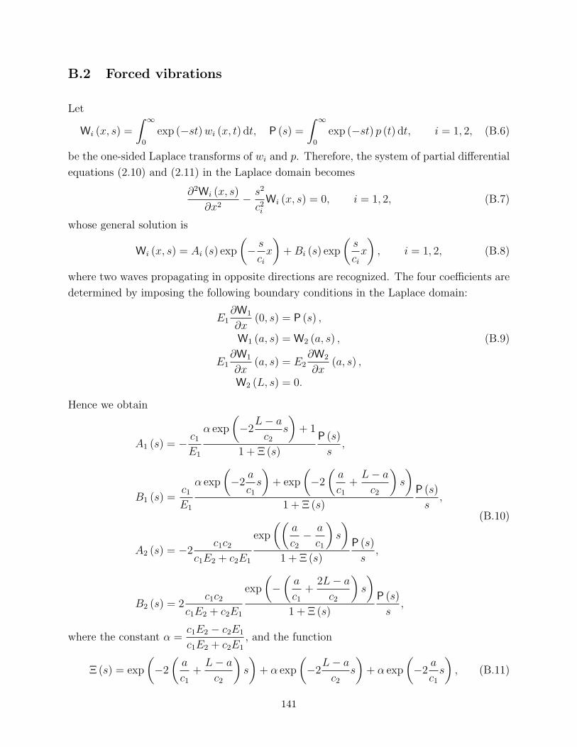
B.2 Forced vibrations
Let
Wi (x, s) =
∫ ∞
0
exp (−st) wi (x, t) dt, P (s) =
∫ ∞
0
exp (−st) p (t) dt, i = 1, 2, (B.6)
be the one-sided Laplace transforms of wi and p. Therefore, the system of partial differential
equations (2.10) and (2.11) in the Laplace domain becomes
∂2Wi (x, s)
∂x2− s2
c2i
Wi (x, s) = 0, i = 1, 2, (B.7)
whose general solution is
Wi (x, s) = Ai (s) exp
(− s
ci
x
)+ Bi (s) exp
(s
ci
x
), i = 1, 2, (B.8)
where two waves propagating in opposite directions are recognized. The four coefficients are
determined by imposing the following boundary conditions in the Laplace domain:
E1∂W1
∂x(0, s) = P (s) ,
W1 (a, s) = W2 (a, s) , (B.9)
E1∂W1
∂x(a, s) = E2
∂W2
∂x(a, s) ,
W2 (L, s) = 0.
Hence we obtain
A1 (s) = − c1
E1
α exp
(−2
L− a
c2
s
)+ 1
1 + Ξ (s)
P (s)
s,
B1 (s) =c1
E1
α exp
(−2
a
c1
s
)+ exp
(−2
(a
c1
+L− a
c2
)s
)
1 + Ξ (s)
P (s)
s,
A2 (s) = −2c1c2
c1E2 + c2E1
exp
((a
c2
− a
c1
)s
)
1 + Ξ (s)
P (s)
s,
B2 (s) = 2c1c2
c1E2 + c2E1
exp
(−
(a
c1
+2L− a
c2
)s
)
1 + Ξ (s)
P (s)
s,
(B.10)
where the constant α =c1E2 − c2E1
c1E2 + c2E1
, and the function
Ξ (s) = exp
(−2
(a
c1
+L− a
c2
)s
)+ α exp
(−2
L− a
c2
s
)+ α exp
(−2
a
c1
s
), (B.11)
141

have been introduced. Identifying the term1
1 + Ξ (s)as the sum of the corresponding geo-
metric series, we write
1
1 + Ξ (s)=
∞∑j=0
[−Ξ (s)]j (B.12)
=∞∑
j=0
j∑
k=0
k∑
h=0
(j
k
)(k
h
)(−1)j αk exp
(−2
((j − k + h)a
c1
+(j − h) (L− a)
c2
)s
).
Therefore, solutions are given by
Wi (x, s) = Gi (x, s) P (s) , (B.13)
where
G1 (x, s) =c1
sE1
∞∑j=0
j∑
k=0
k∑
h=0
(j
k
)(k
h
)(B.14)
(−1)j+1
[αk+1 exp
(−2
((j − k + h)a
c1
+(j − h + 1) (L− a)
c2
+x
2c1
)s
)+
αk exp
(−2
((j − k + h)a
c1
+(j − h) (L− a)
c2
+x
2c1
)s
)]+
(−1)j
[αk+1 exp
(−2
((j − k + h + 1)a
c1
+(j − h) (L− a)
c2
− x
2c1
)s
)+
αk exp
(−2
((j − k + h + 1)a
c1
+(j − h + 1) (L− a)
c2
− x
2c1
)s
)],
and
G2 (x, s) =2c1c2
s (c1E2 + c2E1)
∞∑j=0
j∑
k=0
k∑
h=0
(j
k
)(k
h
)αk (B.15)
(−1)j+1 exp
(−2
((j − k + h)a
c1
+(j − h) (L− a)
c2
+x− a
2c2
+a
2c1
)s
)+
(−1)j exp
(−2
((j − k + h)a
c1
+(j − h) (L− a)
c2
+a
2c1
+2L− a− x
2c2
)s
),
are the transfer functions. From the shifting theorem in the real domain (see, e.g., Meirovitch
(2001)) the inverse Laplace transforms g1 (x, t) and g2 (x, t) of the transfer functions are easily
found. Using the convolution theorem (see, e.g., Meirovitch (2001)), the axial deflections in
the time domain are given by
wi (x, t) =
∫ t
0
gi (x, t− ϑ) p (ϑ) dϑ, i = 1, 2.
142
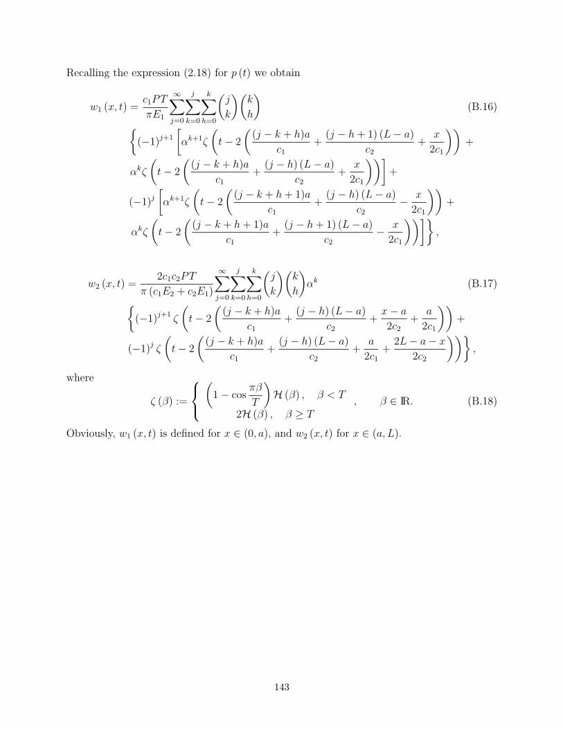
Recalling the expression (2.18) for p (t) we obtain
w1 (x, t) =c1PT
πE1
∞∑j=0
j∑
k=0
k∑
h=0
(j
k
)(k
h
)(B.16)
(−1)j+1
[αk+1ζ
(t− 2
((j − k + h)a
c1
+(j − h + 1) (L− a)
c2
+x
2c1
))+
αkζ
(t− 2
((j − k + h)a
c1
+(j − h) (L− a)
c2
+x
2c1
))]+
(−1)j
[αk+1ζ
(t− 2
((j − k + h + 1)a
c1
+(j − h) (L− a)
c2
− x
2c1
))+
αkζ
(t− 2
((j − k + h + 1)a
c1
+(j − h + 1) (L− a)
c2
− x
2c1
))],
w2 (x, t) =2c1c2PT
π (c1E2 + c2E1)
∞∑j=0
j∑
k=0
k∑
h=0
(j
k
)(k
h
)αk (B.17)
(−1)j+1 ζ
(t− 2
((j − k + h)a
c1
+(j − h) (L− a)
c2
+x− a
2c2
+a
2c1
))+
(−1)j ζ
(t− 2
((j − k + h)a
c1
+(j − h) (L− a)
c2
+a
2c1
+2L− a− x
2c2
)),
where
ζ (β) :=
(1− cos
πβ
T
)H (β) , β < T
2H (β) , β ≥ T, β ∈ IR. (B.18)
Obviously, w1 (x, t) is defined for x ∈ (0, a), and w2 (x, t) for x ∈ (a, L).
143

Appendix C
Method of moments
The potential φ for an arbitrary charge distribution per unit surface, ρS, is given by
φ (y, z) = − 1
2πε0εr
∫
Γ
ρS (θ, ζ) ln ‖(y, z)− (θ, ζ)‖ dΓ + CT, (C.1)
where ‖(y, z)− (θ, ζ)‖ =√
(y − θ)2 + (z − ζ)2 is the distance from the source point (θ, ζ) to
the observation point (y, z), Γ is the overall boundary of the conductors, and CT is a constant
that may be neglected since it does not affect the charge distribution. Boundary conditions
on the top and the bottom rectangle, say Γt and Γb, are φ = V and φ = 0 respectively.
The boundary of each plate is subdivided into small elements and the charge density, ρSi, is
assumed to be constant in element i (piecewise constant basis functions). For convenience
we use the same mesh of Ne elements for the two identical rectangles. By substituting the
charge density approximation into (C.1), and by imposing the boundary conditions at the
geometric centers Pi of the 2Ne elements (collocation method), we obtain the following linear
system of 2Ne equations in 2Ne unknowns collected in the vector ρS:
L ρS = g. (C.2)
The generic entry of the coefficient matrix L is given by:
i = j : Lii = ∆Γi (ln (∆Γi/2)− 1) , (C.3)
i 6= j : Lij = −∆Γj
(1− ln
∥∥∥P(2)j − Pi
∥∥∥)−
∥∥∥P(1)j − Pi
∥∥∥ cos βij ln
∥∥∥P(2)j − Pi
∥∥∥∥∥∥P
(1)j − Pi
∥∥∥(C.4)
+ αij
∥∥∥P(1)j − Pi
∥∥∥ sin βij, (C.5)
where ∆Γi is the length of the i-th element, P(1)j and P
(2)j are the extrema of the j-th element,
βij is the angle between the segments P(1)j P
(2)j and P
(1)j Pi, and αij is the angle between the
segments PiP(2)j and PiP
(1)j . We note that these angles can be computed by using Carnot’s
144

theorem. The element of the vector g equals V if it refers to an element of Γt, and 0 if it refers
to an element of Γb. From the knowledge of the distributed charge per unit surface area, the
charge stored per unit line in each plate may be directly computed, and the capacitance per
unit line estimated.
145

Appendix D
Constitutive relations for hyperelasticand Mooney-Rivlin materials
For an isotropic hyperelastic material the strain energy density (per unit volume in the
reference configuration) function can be written as
W (F) = W (I1, I2, I3) , (D.1)
where I1, I2, I3 are principal invariants of the right Cauchy-Green strain tensor C, and F
is the deformation gradient. From the strain energy function, one obtains the following
expression for the second Piola-Kirchhoff stress tensor.
S =2∂W
∂I1
1+2∂W
∂I2
(I11−C) + 2∂W
∂I3
I3C−1. (D.2)
For incompressible materials the deformation gradient must satisfy the constraint
detF = J = 1, (D.3)
at each point of the body. Because of the constraint (D.3) derivatives of the strain energy
density with respect to the three principal invariants are not independent and the strain
energy density is modified as follows to accommodate the constraint:
W (F) = W (I1, I2) + p (J − 1) , (D.4)
where p is called the pressure that can not be determined from the deformation of the body.
Hence for the stress tensor we have
S =2
(∂W
∂I1
∂I1
∂C+
∂W
∂I2
∂I2
∂C
)+ pC−1. (D.5)
For nearly incompressible isotropic hyperelastic materials the stored energy function may be
written as (see, e.g., Bathe (1996)):
W (C,p) = W (C) + Q (C,p) , (D.6)
146

where
J1 = I1 (I3)−1/3 , J2 = I2 (I3)
−2/3 , (D.7)
and
W (C) = W1 (J1, J2) + W2 (J) , W2 (J) = kG (J) , (D.8)
Q (C,p) = − 1
2k(p (J)− p)2 , p = −dW2
dJ= −k
dG
dJ. (D.9)
Here W1 and W2 are the strain energy densities depending on the distortional and the dilata-
tional deformations respectively, k describes the degree of compressibility, the function G
vanishes only for isochoric deformations, and p is the pressure computed from the deforma-
tion gradient. Formally, when k →∞ the material becomes incompressible. The parameters
J1, J2 are the reduced invariants proposed by Penn (1970) to separate the deformation into
distortional and dilatational parts. Following this decomposition, the second Piola-Kirchhoff
stress tensor is written as
S =2∂W
∂C= 2
(∂W
∂C+
∂Q
∂C
)= S− 2
k(p− p)
∂p
∂C, S =2
∂W
∂C. (D.10)
The contribution to the stress field from displacements only may be rewritten as:
S =2
(∂W1
∂J1
∂J1
∂C+
∂W2
∂J2
∂J2
∂C− p
∂J
∂C
). (D.11)
By computing the derivatives of the reduced invariants with respect to the strain tensor, and
by introducing the quantities
K1 =∂W1
∂J1
, K2 =∂W1
∂J2
, (D.12)
the tensor S becomes
S =2
(K1I
−1/33
(I− 1
3I1C
−1
)+ K2I
−2/33
(I1I−C−2
3I2C
−1
))− JpC−1, (D.13)
where we used the relations
∂I1
∂C= I,
∂I2
∂C= I1I−C,
∂I3
∂C= I3C
−1. (D.14)
For nearly incompressible materials several forms of the strain energy function are available
in the literature, see, e.g., Peng and Chang (1997). Following Chen, Pan and Wu (1997) we
use
W1 =∞∑
m+n=1
Amn (J1 − 3)m (J2 − 3)n , (D.15a)
G =1
2(J − 1)2 . (D.15b)
147
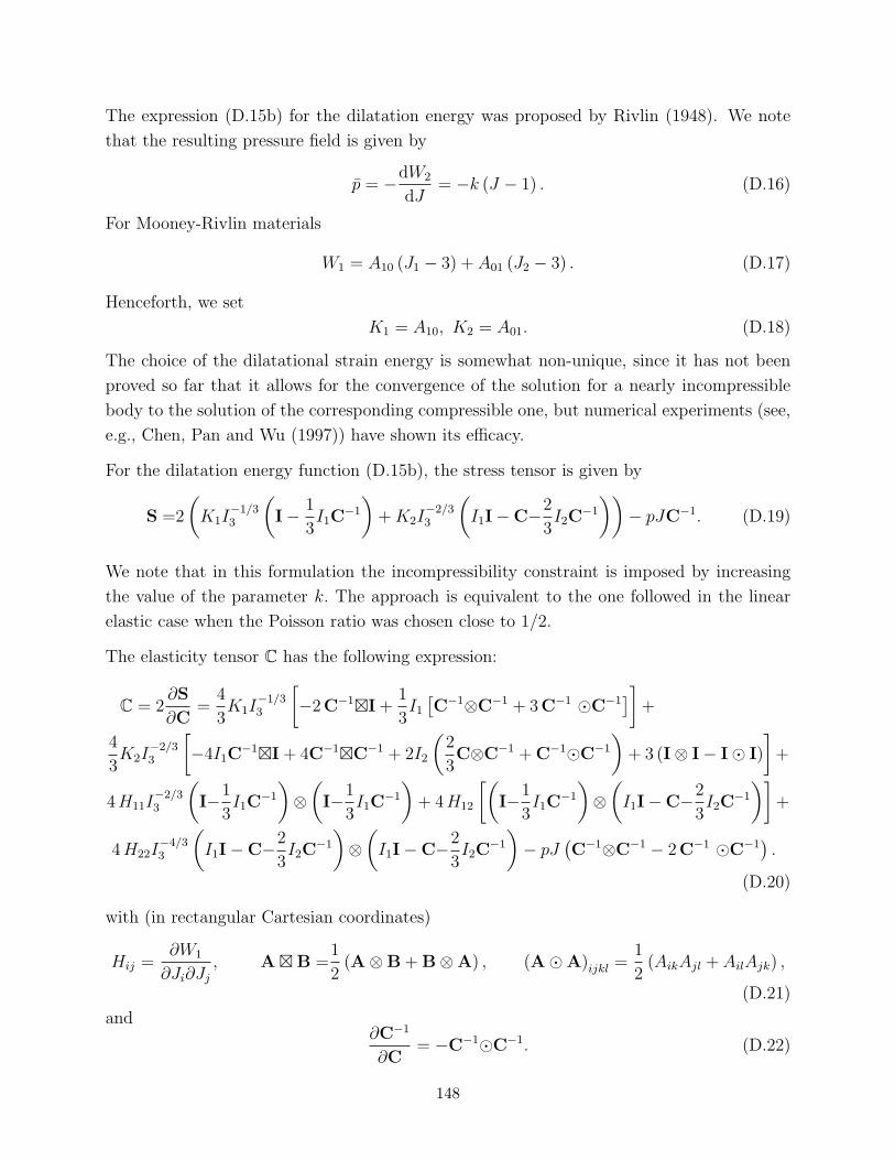
The expression (D.15b) for the dilatation energy was proposed by Rivlin (1948). We note
that the resulting pressure field is given by
p = −dW2
dJ= −k (J − 1) . (D.16)
For Mooney-Rivlin materials
W1 = A10 (J1 − 3) + A01 (J2 − 3) . (D.17)
Henceforth, we set
K1 = A10, K2 = A01. (D.18)
The choice of the dilatational strain energy is somewhat non-unique, since it has not been
proved so far that it allows for the convergence of the solution for a nearly incompressible
body to the solution of the corresponding compressible one, but numerical experiments (see,
e.g., Chen, Pan and Wu (1997)) have shown its efficacy.
For the dilatation energy function (D.15b), the stress tensor is given by
S =2
(K1I
−1/33
(I− 1
3I1C
−1
)+ K2I
−2/33
(I1I−C−2
3I2C
−1
))− pJC−1. (D.19)
We note that in this formulation the incompressibility constraint is imposed by increasing
the value of the parameter k. The approach is equivalent to the one followed in the linear
elastic case when the Poisson ratio was chosen close to 1/2.
The elasticity tensor C has the following expression:
C = 2∂S
∂C=
4
3K1I
−1/33
[−2C−1£I +
1
3I1
[C−1⊗C−1 + 3C−1 ¯C−1
]]+
4
3K2I
−2/33
[−4I1C
−1£I + 4C−1£C−1 + 2I2
(2
3C⊗C−1 + C−1¯C−1
)+ 3 (I⊗ I− I¯ I)
]+
4 H11I−2/33
(I−1
3I1C
−1
)⊗
(I−1
3I1C
−1
)+ 4 H12
[(I−1
3I1C
−1
)⊗
(I1I−C−2
3I2C
−1
)]+
4 H22I−4/33
(I1I−C−2
3I2C
−1
)⊗
(I1I−C−2
3I2C
−1
)− pJ
(C−1⊗C−1 − 2C−1 ¯C−1
).
(D.20)
with (in rectangular Cartesian coordinates)
Hij =∂W1
∂Ji∂Jj
, A £ B =1
2(A⊗B + B⊗A) , (A¯A)ijkl =
1
2(AikAjl + AilAjk) ,
(D.21)
and∂C−1
∂C= −C−1¯C−1. (D.22)
148

Similarly the tensor H relating the incremental stress to the incremental pressure, and the
tensor Q are given by
H =∂S
∂p= −JC−1, Q = 2
∂p
∂C= −kJC−1 ≡ kH. (D.23)
Expressions for tensors C, H and Q for a natural reference configuration are
C =4
3(K1 + K2) (3I¯ I− I⊗ I) , H =− I, Q = −kI. (D.24)
Therefore, for infinitesimal deformations the material behaves as an isotropic linear elastic
with constitutive parameters
ν =1
2
(1− 2
K1 + K2
k
), E =
(6− 4
K1 + K2
k
)(K1 + K2) . (D.25)
149
Vita
Maurizio Porfiri was born on November 19, 1976 in Rome, Italy. In 2000, he received the
Master of Science degree in Engineering Mechanics from the Virginia Polytechnic Institute
and State University, Blacksburg, USA; in 2001 he earned the ”Laurea” degree in Electrical
Engineering with honours from the University of Rome ”La Sapienza”, Rome, Italy; in
2005 he was awarded with the Ph.D. degree in Theoretical and Applied Mechanics from the
University of Rome ”La Sapienza” and with the Ph.D. in Mechanics from the University
of Toulon et du Var, Toulon, France. In addition, from July 2005 to June 2006, he was a
postdoctoral associate in the Bradley Department of Electrical and Computer Engineering
at the Virginia Polytechnic Institute and State University.
150


![Meshless Local Petrov-Galerkin (MLPG) Method for ... · [O˜nate, Idelsohn, Zienkiewicz, and Taylor (1996)] is a truly meshless method. A non-element interpolation scheme - weighted](https://img.dokumen.tips/doc/110x75/5f38124645c728780d7dd2b1/meshless-local-petrov-galerkin-mlpg-method-for-ooenate-idelsohn-zienkiewicz.jpg)