Analysis and Geometry on GraphsPart 1. Laplace operator on weighted graphs

Alexander Grigor’yan

Tsinghua University, Winter 2012

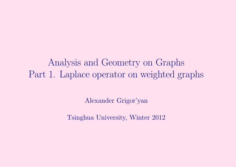
1 Weighted graphs and Markov chains

The notion of a graph. A graph is a couple (V,E) where V is a setof vertices, that is, an arbitrary set, whose elements are called vertices,and E is a set of edges, that is, E consists of some couples (x, y) wherex, y ∈ V . We write x ∼ y (x is connected to y, or x is joint to y, or x isadjacent to y, or x is a neighbor of y ) if (x, y) ∈ E. The edge (x, y) willbe normally denoted by xy. In this section we assume that the graphsare undirected so that xy ≡ yx. The vertices x, y are called the endpointsof the edge xy. The edge xx with the same endpoints (should it exist)is called a loop. Generally we allow loops although in the most examplesour graphs do not have loops.

A graph (V,E) is called finite if the number #V of vertices is finite. Inthis course all graphs are finite unless otherwise stated. For each vertexx, define its degree

deg (x) = # {y ∈ V : x ∼ y} ,

that is, deg (x) is the number of neighbors of x. A graph is called regularif deg (x) is the same for all x ∈ V .

1

Example. Consider some examples of graphs.

1. A complete graph Kn. The set of vertices is V = {1, 2, ..., n}, andthe edges are defined as follows: i ∼ j for any two distinct i, j ∈ V .

2. A complete bipartite graph Kn,m. The set of vertices is V ={1, .., n, n + 1, ..., n + m}, and the edges are defined as follows: i ∼j if either i < n and j ≥ n or i ≥ n and j < n. That is,the set of vertices is split into two groups: V1 = {1, ..., n} andV2 = {n + 1, ...,m}, and the vertices are connected if and only ifthey belong to the different groups.

3. A cycle graph, denoted by Zm. The set of vertices is the set ofresidues mod m that is, V = {0, 1, ...,m − 1}, and i ∼ j if i − j =±1 mod m.

4. A path graph Pm. The set of vertices is V = {0, 1, ...,m − 1}, andi ∼ j if |i − j| = 1.

For example,K2 = K1,1 = Z2 = P2 = • − •

2

Z3 =•

� |• − •

, Z4 = K2,2 =• − •| |• − •

Product of graphs. More interesting examples of graphs can be con-structed using the operation of product of graphs.

Definition. Let (X,E1) and (Y,E2) be two graphs. Their Cartesianproduct is defined as follows:

(V,E) = (X,E1)� (Y,E2)

where V = X × Y is the set of pairs (x, y) where x ∈ X and y ∈ Y , andthe set E of edges is defined by

(x, y) ∼ (x′, y) if x′ ∼ x and (x, y) ∼ (x, y′) if y ∼ y′, (1.1)

3

which is illustrated on the following diagram:

y′• . . .(x,y′)• −

(x′,y′)• . . .

| | |

y• . . .(x,y)• −

(x′,y)• . . .

......

...Y�X . . . x• − x′• . . .

Clearly, we have #V = (#X) (#Y ) and deg (x, y) = deg (x)+deg (y) forall x ∈ X and y ∈ Y .

For example, we have

Z2�Z2 = Z4 =• − •| |• − •

, P4�P3 =

• − • − • − •| | | |• − • − • − •| | | |• − • − • − •

This definition can be iterated to define the product of a finite se-

4

quence of graphs. The graph Zn2 := Z2�Z2�...�Z2︸ ︷︷ ︸

n

is called the n-

dimensional binary cube. For example,

Z32 =

• − − − − − •| � � || • − • || | | || • − • || � � |• − − − − − •

The graph distance.

Definition. A finite sequence {xk}nk=0 of vertices on a graph is called a

path if xk ∼ xk+1 for all k = 0, 1, ..., n− 1. The number n of edges in thepath is referred to as the length of the path.

Definition. A graph (V,E) is called connected if, for any two verticesx, y ∈ V , there is a path connecting x and y, that is, a path {xk}

nk=0

such that x0 = x and xn = y. If (V,E) is connected then define the

5

graph distance d (x, y) between any two distinct vertices x, y as follows:if x 6= y then d (x, y) is the minimal length of a path that connects x andy, and if x = y then d (x, y) = 0.

The connectedness here is needed to ensure that d (x, y) < ∞ for anytwo points. It is easy to see that on any connected graph, the graphdistance is a metric, so that (V, d) is a metric space.

Weighted graphs.

Definition. A weighted graph is a couple ((V,E) , μ) where (V,E) is agraph and μxy is a non-negative function on V × V such that

1. μxy = μyx;

2. μxy > 0 if and only if x ∼ y.

The weighted graph can also be denoted by (V, μ) because the weightμ contains all information about the set of edges E.

Example. Set μxy = 1 if x ∼ y and μxy = 0 otherwise. Then μxy is aweight. This specific weight is called simple.

6

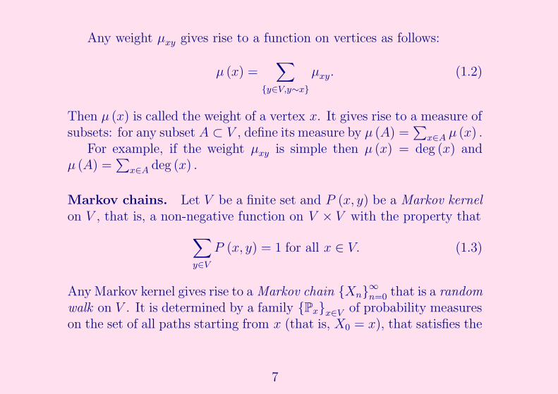
Any weight μxy gives rise to a function on vertices as follows:

μ (x) =∑

{y∈V,y∼x}

μxy. (1.2)

Then μ (x) is called the weight of a vertex x. It gives rise to a measure ofsubsets: for any subset A ⊂ V , define its measure by μ (A) =

∑x∈A μ (x) .

For example, if the weight μxy is simple then μ (x) = deg (x) andμ (A) =

∑x∈A deg (x) .

Markov chains. Let V be a finite set and P (x, y) be a Markov kernelon V , that is, a non-negative function on V × V with the property that

∑

y∈V

P (x, y) = 1 for all x ∈ V. (1.3)

Any Markov kernel gives rise to a Markov chain {Xn}∞n=0 that is a random

walk on V . It is determined by a family {Px}x∈V of probability measureson the set of all paths starting from x (that is, X0 = x), that satisfies the

7

following property: for all positive integers n and all x, x1, ..., xn ∈ V ,

Px (X1 = x1, X2 = x2, ..., Xn = xn) = P (x, x1) P (x1, x2) ...P (xn−1, xn) .(1.4)

In other words, if X0 = x then the probability that the walk {Xn} visitssuccessively the vertices x1, x2, ..., xn is equal to the right hand side of(1.4).

•x1 x3• xn•

↗ ↘ ↗. . . . . .

. . . ↗x• •x2 xn−1•

For any positive integer n and any x ∈ V , set

Pn (x, y) = Px (Xn = y) .

The function Pn (x, y) is called the transition function or the transitionprobability of the Markov chain. For a fixed n and x ∈ V , the func-tion Pn (x, ∙) nothing other than the distribution measure of the randomvariable Xn.

8

For n = 1 we obtain from (1.4) P1 (x, y) = P (x, y). Let us statewithout proofs some easy consequences of (1.4).

1. For all x, y ∈ V and positive integer n,

Pn+1 (x, y) =∑

z∈V

Pn (x, z) P (z, y) . (1.5)

2. Moreover, for all positive integers n, k,

Pn+k (x, y) =∑

z∈V

Pn (x, z) Pk (z, y) . (1.6)

3. Pn (x, y) is also a Markov kernel, that is,

∑

y∈V

Pn (x, y) = 1. (1.7)

9

Reversible Markov chains. Let (V, μ) be a finite weighted graphwithout isolated vertices (the latter is equivalent to μ (x) > 0). Theweight μ induces a natural Markov kernel

P (x, y) =μxy

μ (x). (1.8)

Since μ (x) =∑

y∈V μxy, we see that∑

y P (x, y) ≡ 1 so that P (x, y)is indeed a Markov kernel. For example, if μ is a simple weight thenμ (x) = deg (x) and

P (x, y) =

{ 1deg(x)

, y ∼ x,

0, y 6∼ x.(1.9)

The Markov kernel (1.8) has an additional specific property

P (x, y) μ (x) = P (y, x) μ (y) , (1.10)

that follows from μxy = μyx.

Definition. An arbitrary Markov kernel P (x, y) is called reversible ifthere is a positive function μ (x) with the property (1.10). Function μ iscalled then the invariant measure of P .

10

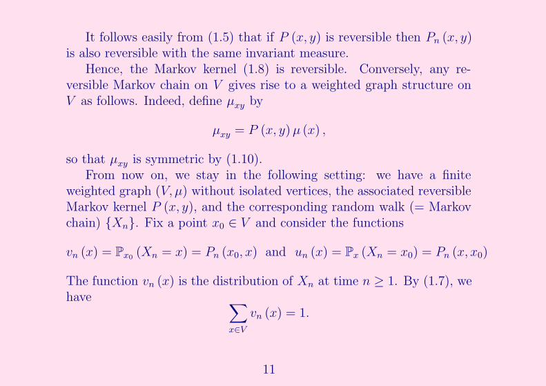
It follows easily from (1.5) that if P (x, y) is reversible then Pn (x, y)is also reversible with the same invariant measure.

Hence, the Markov kernel (1.8) is reversible. Conversely, any re-versible Markov chain on V gives rise to a weighted graph structure onV as follows. Indeed, define μxy by

μxy = P (x, y) μ (x) ,

so that μxy is symmetric by (1.10).From now on, we stay in the following setting: we have a finite

weighted graph (V, μ) without isolated vertices, the associated reversibleMarkov kernel P (x, y), and the corresponding random walk (= Markovchain) {Xn}. Fix a point x0 ∈ V and consider the functions

vn (x) = Px0 (Xn = x) = Pn (x0, x) and un (x) = Px (Xn = x0) = Pn (x, x0)

The function vn (x) is the distribution of Xn at time n ≥ 1. By (1.7), wehave ∑

x∈V

vn (x) = 1.

11

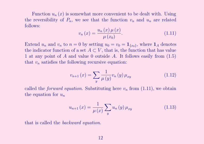
Function un (x) is somewhat more convenient to be dealt with. Usingthe reversibility of Pn, we see that the function vn and un are relatedfollows:

vn (x) =un (x) μ (x)

μ (x0). (1.11)

Extend un and vn to n = 0 by setting u0 = v0 = 1{x0}, where 1A denotesthe indicator function of a set A ⊂ V , that is, the function that has value1 at any point of A and value 0 outside A. It follows easily from (1.5)that vn satisfies the following recursive equation:

vn+1 (x) =∑

y

1

μ (y)vn (y) μxy (1.12)

called the forward equation. Substituting here vn from (1.11), we obtainthe equation for un

un+1 (x) =1

μ (x)

∑

y

un (y) μxy (1.13)

that is called the backward equation.

12

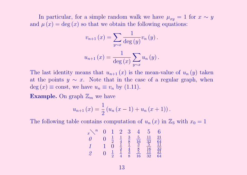
In particular, for a simple random walk we have μxy = 1 for x ∼ yand μ (x) = deg (x) so that we obtain the following equations:

vn+1 (x) =∑

y∼x

1

deg (y)vn (y) .

un+1 (x) =1

deg (x)

∑

y∼x

un (y) .

The last identity means that un+1 (x) is the mean-value of un (y) takenat the points y ∼ x. Note that in the case of a regular graph, whendeg (x) ≡ const, we have un ≡ vn by (1.11).

Example. On graph Zm we have

un+1 (x) =1

2(un (x − 1) + un (x + 1)) .

The following table contains computation of un (x) in Z3 with x0 = 1

x�n 0 1 2 3 4 5 60 0 1

214

38

516

1132

2164

1 1 0 12

14

38

516

1132

2 0 12

14

38

516

1132

2164

13

Here one can observe that the function un (x) converges to a constantfunction 1/3 as n → ∞ and later we will prove this. Hence, for large n,the probability that Xn visits a given point is nearly 1/3, which shouldbe expected.

Here are the values of un (x) in Z5 with x0 = 2:

x�n 0 1 2 3 4 . . . 250 0 0 1

418

14

. . . 0.1991 0 1

20 3

8116

. . . 0.2022 1 0 1

20 3

8. . . 0.198

3 0 12

0 38

116

. . . 0.2024 0 0 1

418

14

. . . 0.199

Here un (x) approaches to 15

as n → 5 but the convergence is slower thanin the case of Z3.

Example. On a complete graph Km we have

un+1 (x) =1

m − 1

∑

y 6=x

un (y) .

14

Here are the values of un (x) on K5 with x0 = 2:

x�n 0 1 2 3 40 0 1

4316

1364

0.1991 0 1

4316

1364

0.1992 1 0 1

4316

0.2033 0 1

4316

1364

0.1994 0 1

4316

1364

0.199

We see that un (x) → 15

but the rate of convergence is much faster thanfor Z5. Although Z5 and K5 has the same number of vertices, the extraedges in K5 allow a quicker mixing than in the case of Z5.

As we will see, for finite graphs it is typically the case that the transi-tion function un (x) converges to a constant as n → ∞. For the functionvn this means that

vn (x) =un (x) μ (x)

μ0 (x)→ cμ (x) as n → ∞

for some constant c. The constant c is determined by the requirement

15

that cμ (x) is a probability measure on V , that is, from the identity

c∑

x∈V

μ (x) = 1.

Hence, cμ (x) is asymptotically the distribution of Xn as n → ∞. . Thefunction cμ (x) on V is called the stationary measure or the equilibriummeasure of the Markov chain. One of the problems for finite graphs thatwill be discussed in this course, is the rate of convergence of vn (x) to theequilibrium measure. The point is that Xn can be considered for largen as a random variable with the distribution function cμ (x) so that weobtain a natural generator of a random variable with a prescribed law.However, in order to be able to use this, one should know for which nthe distribution of Xn is close enough to the equilibrium measure. Thevalue of n, for which this is the case, is called the mixing time.

16

2 The Laplace operator

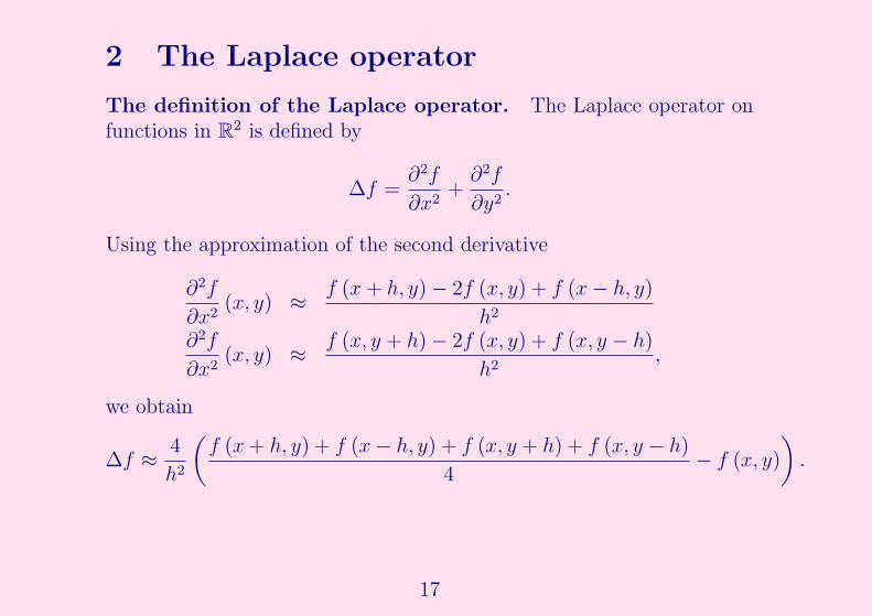
The definition of the Laplace operator. The Laplace operator onfunctions in R2 is defined by

Δf =∂2f

∂x2+

∂2f

∂y2.

Using the approximation of the second derivative

∂2f

∂x2(x, y) ≈

f (x + h, y) − 2f (x, y) + f (x − h, y)

h2

∂2f

∂x2(x, y) ≈

f (x, y + h) − 2f (x, y) + f (x, y − h)

h2,

we obtain

Δf ≈4

h2

(f (x + h, y) + f (x − h, y) + f (x, y + h) + f (x, y − h)

4− f (x, y)

)

.

17

Restricting f to the grid hZ2 and define the edges in hZ2 as on theproduct graph, we see that

Δf (x, y) ≈4

h2

1

4

∑

(x′,y′)∼(x,y)

f (x′, y′) − f (x, y)

.

The expression in the parenthesis is called the discrete Laplace operatoron hZ2.

This notion can be defined on any weighted graph as follows.

Definition. Let (V, μ) be a finite weighted graph without isolated points.For any function f : V → R, define the function Δμf by

Δμf (x) =1

μ (x)

∑

y∼x

f (y) μxy − f (x) . (2.1)

The operator Δμ is called the (weighted) Laplace operator of (V, μ).

This operator can also be written in equivalent forms as follows:

Δμf (x) =1

μ (x)

∑

y∈V

f (y) μxy − f (x) =1

μ (x)

∑

y∈V

(f (y) − f (x)) μxy.

(2.2)

18

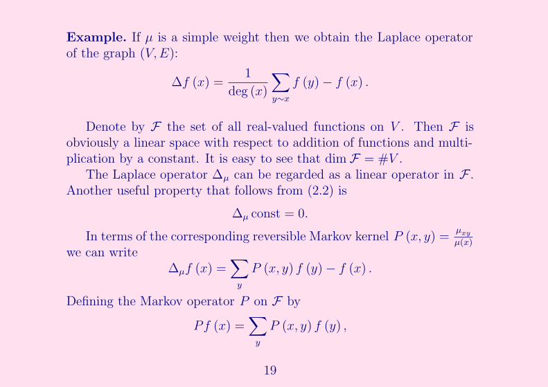
Example. If μ is a simple weight then we obtain the Laplace operatorof the graph (V,E):

Δf (x) =1

deg (x)

∑

y∼x

f (y) − f (x) .

Denote by F the set of all real-valued functions on V . Then F isobviously a linear space with respect to addition of functions and multi-plication by a constant. It is easy to see that dim F = #V .

The Laplace operator Δμ can be regarded as a linear operator in F .Another useful property that follows from (2.2) is

Δμ const = 0.

In terms of the corresponding reversible Markov kernel P (x, y) =μxy

μ(x)

we can writeΔμf (x) =

∑

y

P (x, y) f (y) − f (x) .

Defining the Markov operator P on F by

Pf (x) =∑

y

P (x, y) f (y) ,

19

we see that the Laplace operator Δμ and the Markov operator P arerelated by a simple identity Δμ = P−id, where id is the identity operatorin F .

Green’s formula. Let us consider the difference operator ∇xy that isdefined for any two vertices x, y ∈ V and maps F to R as follows:

∇xyf = f (y) − f (x) .

The relation between the Laplace operator Δμ and the difference operatoris given by

Δμf (x) =1

μ (x)

∑

y

(∇xyf) μxy =∑

y

P (x, y) (∇xyf)

The following theorem is one of the main tools when working with theLaplace operator. For any subset Ω of V , denote by Ωc the complementof Ω, that is, Ωc = V \ Ω.

20

Theorem 2.1 (Green’s formula) Let (V, μ) be a finite weighted graphwithout isolated points, and let Ω be a non-empty finite subset of V .Then, for any two functions f, g on V ,

∑

x∈Ω

Δμf(x)g(x)μ(x) = −1

2

∑

x,y∈Ω

(∇xyf) (∇xyg) μxy+∑

x∈Ω,y∈Ωc

(∇xyf) g(x)μxy

(2.3)

The formula (2.3) is analogous to the Green formula for the Laplaceoperator in R2: if Ω is a bounded domain in R2 with smooth boundarythen, for all smooth enough functions f, g on Ω

∫

Ω

(Δf) gdx = −∫

Ω

∇f ∙ ∇gdx +

∫

∂Ω

∂f

∂νgd`

where ν is the unit normal vector field on ∂Ω and d` is the length elementon ∂Ω.

If Ω = V then Ωc is empty so that the last “boundary” term in (2.3)vanishes, and we obtain

∑

x∈V

Δμf(x)g(x)μ(x) = −1

2

∑

x,y∈V

(∇xyf) (∇xyg) μxy. (2.4)

21

Proof. We have

∑

x∈Ω

Δμf(x)g(x)μ(x) =∑

x∈Ω

(1

μ (x)

∑

y∈V

(∇xyf) μxy

)

g(x)μ(x)

=∑

x∈Ω

∑

y∈V

(∇xyf) g(x)μxy

=∑

x∈Ω

∑

y∈Ω

(∇xyf) g(x)μxy +∑

x∈Ω

∑

y∈Ωc

(∇xyf) g(x)μxy

=∑

y∈Ω

∑

x∈Ω

(∇yxf) g(y)μxy +∑

x∈Ω

∑

y∈Ωc

(∇xyf) g(x)μxy,

where in the last line we have switched notation of the variables x and yin the first sum using μxy = μyx. Adding together the last two lines anddividing by 2, we obtain

∑

x∈Ω

Δμf(x)g(x)μ(x) =1

2

∑

x,y∈Ω

(∇xyf) (g(x) − g(y)) μxy+∑

x∈Ωy∈Ωc

(∇xyf) g(x)μxy,

which was to be proved.

22

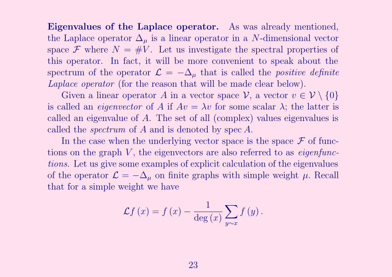
Eigenvalues of the Laplace operator. As was already mentioned,the Laplace operator Δμ is a linear operator in a N -dimensional vectorspace F where N = #V . Let us investigate the spectral properties ofthis operator. In fact, it will be more convenient to speak about thespectrum of the operator L = −Δμ that is called the positive definiteLaplace operator (for the reason that will be made clear below).

Given a linear operator A in a vector space V , a vector v ∈ V \ {0}is called an eigenvector of A if Av = λv for some scalar λ; the latter iscalled an eigenvalue of A. The set of all (complex) values eigenvalues iscalled the spectrum of A and is denoted by spec A.

In the case when the underlying vector space is the space F of func-tions on the graph V , the eigenvectors are also referred to as eigenfunc-tions. Let us give some examples of explicit calculation of the eigenvaluesof the operator L = −Δμ on finite graphs with simple weight μ. Recallthat for a simple weight we have

Lf (x) = f (x) −1

deg (x)

∑

y∼x

f (y) .

23

Example. 1. For graph Z2 we have

Lf (0) = f (0) − f (1)

Lf (1) = f (1) − f (0)

so that the equation Lf = λf becomes

(1 − λ) f (0) = f (1)

(1 − λ) f (1) = f (0)

whence (1 − λ)2 f (k) = f (k) for both k = 0, 1. Since f 6≡ 0, we obtainthe equation (1 − λ)2 = 1 whence we find two eigenvalues λ = 0 andλ1 = 2. Alternatively, considering a function f as a column-vector

(f(0)f(1)

),

we can represent the action of L as a matrix multiplication:(Lf (0)

Lf (1)

)

=

(1 −1−1 1

)(f (0)

f (1)

)

,

so that the eigenvalues of L coincide with those of the matrix

(1 −1−1 1

)

.

Its characteristic equation is (1 − λ)2 − 1 = 0, whence we obtain againthe same two eigenvalues λ = 0 and λ = 2.

24

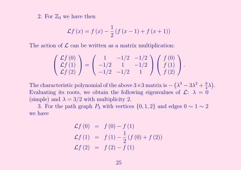
2. For Z3 we have then

Lf (x) = f (x) −1

2(f (x − 1) + f (x + 1))

The action of L can be written as a matrix multiplication:

Lf (0)Lf (1)Lf (2)

=

1 −1/2 −1/2

−1/2 1 −1/2−1/2 −1/2 1

f (0)f (1)f (2)

.

The characteristic polynomial of the above 3×3 matrix is −(λ3 − 3λ2 + 9

4λ).

Evaluating its roots, we obtain the following eigenvalues of L: λ = 0(simple) and λ = 3/2 with multiplicity 2.

3. For the path graph P3 with vertices {0, 1, 2} and edges 0 ∼ 1 ∼ 2we have

Lf (0) = f (0) − f (1)

Lf (1) = f (1) −1

2(f (0) + f (2))

Lf (2) = f (2) − f (1)

25

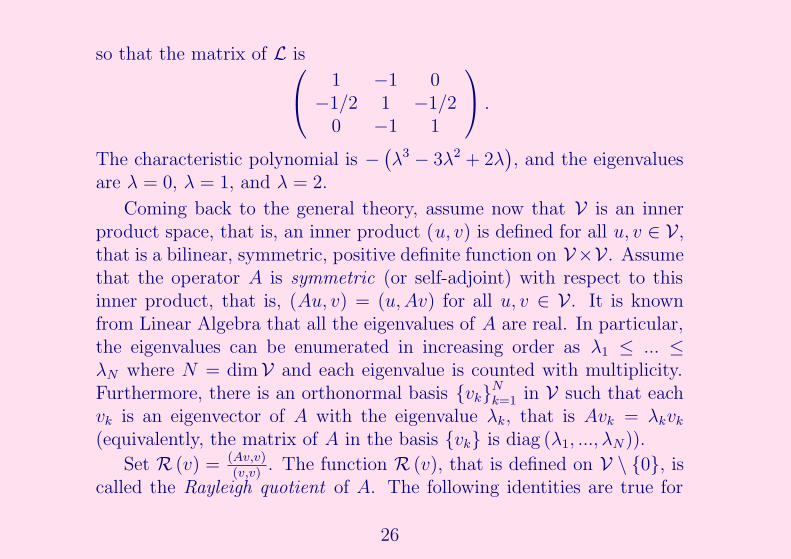
so that the matrix of L is

1 −1 0

−1/2 1 −1/20 −1 1

.

The characteristic polynomial is −(λ3 − 3λ2 + 2λ

), and the eigenvalues

are λ = 0, λ = 1, and λ = 2.

Coming back to the general theory, assume now that V is an innerproduct space, that is, an inner product (u, v) is defined for all u, v ∈ V ,that is a bilinear, symmetric, positive definite function on V×V . Assumethat the operator A is symmetric (or self-adjoint) with respect to thisinner product, that is, (Au, v) = (u,Av) for all u, v ∈ V . It is knownfrom Linear Algebra that all the eigenvalues of A are real. In particular,the eigenvalues can be enumerated in increasing order as λ1 ≤ ... ≤λN where N = dimV and each eigenvalue is counted with multiplicity.Furthermore, there is an orthonormal basis {vk}

Nk=1 in V such that each

vk is an eigenvector of A with the eigenvalue λk, that is Avk = λkvk

(equivalently, the matrix of A in the basis {vk} is diag (λ1, ..., λN)).

Set R (v) = (Av,v)(v,v)

. The function R (v), that is defined on V \ {0}, iscalled the Rayleigh quotient of A. The following identities are true for

26

all k = 1, ..., N :

λk = R (vk) = infv⊥v1,...,vk−1

R (v) = supv⊥vN ,vN−1,...,vk+1

R (v)

(where v⊥u means that u and v are orthogonal, that is, (v, u) = 0). Inparticular,

λ1 = infv 6=0

R (v) and λN = supv 6=0

R (v) .

We will apply these results to the Laplace L in the vector space F ofreal-valued functions on V . Consider in F the following inner product:for any two functions f, g ∈ F , set

(f, g) :=∑

x∈V

f (x) g (x) μ (x) ,

which can be considered as the integration of fg against measure μ onV .

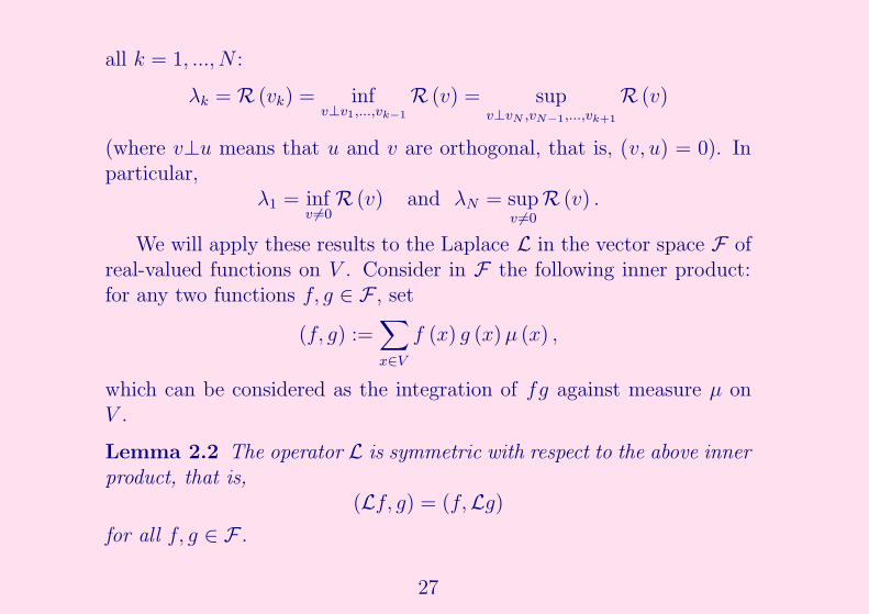
Lemma 2.2 The operator L is symmetric with respect to the above innerproduct, that is,

(Lf, g) = (f,Lg)

for all f, g ∈ F .

27

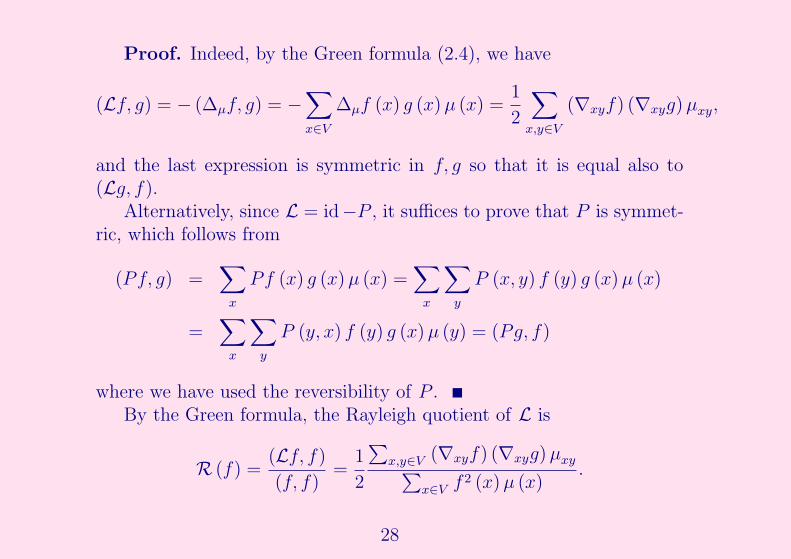
Proof. Indeed, by the Green formula (2.4), we have

(Lf, g) = − (Δμf, g) = −∑

x∈V

Δμf (x) g (x) μ (x) =1

2

∑

x,y∈V

(∇xyf) (∇xyg) μxy,

and the last expression is symmetric in f, g so that it is equal also to(Lg, f ).

Alternatively, since L = id−P , it suffices to prove that P is symmet-ric, which follows from

(Pf, g) =∑

x

Pf (x) g (x) μ (x) =∑

x

∑

y

P (x, y) f (y) g (x) μ (x)

=∑

x

∑

y

P (y, x) f (y) g (x) μ (y) = (Pg, f )

where we have used the reversibility of P .By the Green formula, the Rayleigh quotient of L is

R (f) =(Lf, f)

(f, f)=

1

2

∑x,y∈V (∇xyf) (∇xyg) μxy∑

x∈V f 2 (x) μ (x).

28

To state the next theorem about the spectrum of L, we need a notionof a bipartite graph.

Definition. A graph (V,E) is called bipartite if V admits a partitioninto two non-empty disjoint subsets V1, V2 such that x, y ∈ Vi ⇒ x 6∼ y.

In terms of coloring, one can say that a graph is bipartite if its verticescan be colored by two colors, so that the vertices of the same color arenot connected by an edge.

Example. Here are some examples of bipartite graphs.

1. A complete bipartite graph Kn,m is bipartite.

2. The graphs Zm and Pm is bipartite provided m is even.

3. Product of bipartite graphs is bipartite. In particular, Znm and P n

m

are bipartite provided m is even.

Theorem 2.3 For any finite, connected, weighted graph (V, μ) with N =#V > 1, the following is true.

29

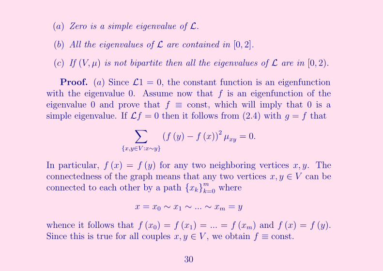
(a) Zero is a simple eigenvalue of L.

(b) All the eigenvalues of L are contained in [0, 2].

(c) If (V, μ) is not bipartite then all the eigenvalues of L are in [0, 2).

Proof. (a) Since L1 = 0, the constant function is an eigenfunctionwith the eigenvalue 0. Assume now that f is an eigenfunction of theeigenvalue 0 and prove that f ≡ const, which will imply that 0 is asimple eigenvalue. If Lf = 0 then it follows from (2.4) with g = f that

∑

{x,y∈V :x∼y}

(f (y) − f (x))2 μxy = 0.

In particular, f (x) = f (y) for any two neighboring vertices x, y. Theconnectedness of the graph means that any two vertices x, y ∈ V can beconnected to each other by a path {xk}

mk=0 where

x = x0 ∼ x1 ∼ ... ∼ xm = y

whence it follows that f (x0) = f (x1) = ... = f (xm) and f (x) = f (y).Since this is true for all couples x, y ∈ V , we obtain f ≡ const.

30

(b) Let λ be an eigenvalue of L with an eigenfunction f . Using Lf =λf and the Green formula (2.4), we obtain

λ∑

x∈V

f 2 (x) μ (x) =∑

x∈V

Lf (x) f (x) μ (x)

=1

2

∑

{x,y∈V :x∼y}

(f (y) − f (x))2 μxy. (2.5)

It follows from (2.5) that λ ≥ 0. Using (a + b)2 ≤ 2 (a2 + b2), we obtain

λ∑

x∈V

f 2 (x) μ (x) ≤∑

{x,y∈V :x∼y}

(f (y)2 + f (x)2)μxy

=∑

x,y∈V

f (y)2 μxy +∑

x,y∈V

f (x)2 μxy

=∑

y∈V

f (y)2 μ (y) +∑

x∈V

f (x)2 μ (x)

= 2∑

x∈V

f (x)2 μ (x) . (2.6)

It follows from (2.6) that λ ≤ 2.

31

Alternatively, one can first prove that ‖P‖ ≤ 1 , which follows from∑y P (x, y) = 1 and which implies spec P ⊂ [−1, 1], and then conclude

that specL = 1 − spec P ⊂ [0, 2] .(c) We need to prove that λ = 2 is not an eigenvalue. Assume from

the contrary that λ = 2 is an eigenvalue with an eigenfunction f , andprove that (V, μ) is bipartite. Since λ = 2, all the inequalities in theabove calculation (2.6) must become equalities. In particular, we musthave for all x ∼ y that

(f (x) − f (y))2 = 2(f (x)2 + f (y)2) ,

which is equivalent tof (x) + f (y) = 0.

If f (x0) = 0 for some x0 then it follows that f (x) = 0 for all neighborsof x0. Since the graph is connected, we obtain that f (x) ≡ 0, which isnot possible for an eigenfunction. Hence, f (x) 6= 0 for all x ∈ Γ. ThenV splits into a disjoint union of two sets:

V + = {x ∈ V : f (x) > 0} and V − = {x ∈ V : f (x) < 0} .

32

The above argument shows that if x ∈ V + then all neighbors of x are inV −, and vice versa. Hence, (V, μ) is bipartite, which finishes the proof.

Hence, we can enumerate all the eigenvalues of L in the increasingorder as follows:

0 = λ0 < λ1 ≤ λ2 ≤ ... ≤ λN−1.

Note that the smallest eigenvalue is denoted by λ0 rather than by λ1.Also, we have always λN−1 ≤ 2 and the latter inequality is strict if thegraph is non-bipartite. Below is a diagram of the interval [0 , 2] withmarked eigenvalues:

|−λ0=0

− •λ1

−−−−•−−−−•−−|1

−−−−•−−•−−−− •−λN−1

−|2

Example. As an example of application of Theorem 2.3, let us investi-gate the solvability of the equation Lu = f. Since by the Green formula

∑

x

(Lu) (x) μ (x) = 0,

33

a necessary condition for solvability is

∑

x

f (x) μ (x) = 0. (2.7)

Assuming that, let us show that the equation Lu = f has a solution.Indeed, condition (2.7) means that f⊥1. Consider the subspace F0 of Fthat consists of all functions orthogonal to 1. Since 1 is the eigenfunctionof L with eigenvalue λ0 = 0, the space F0 is invariant for the operator L,and the spectrum of L in F0 is λ1, ...λN−1. Since all λj > 0, we see thatL is invertible in F0, that is, the equation Lu = f has for any f ∈ F0 aunique solution u ∈ F0 given by u = L−1f .

3 Convergence to equilibrium

The next theorem is one of the main results of this Section. We use thenotation

‖f‖ =√

(f, f).

34

Theorem 3.1 Let (V, μ) be a finite, connected, weighted graph with N =#V > 1. and P be its Markov operator. For any function f ∈ F , set

f =1

μ (V )

∑

x∈V

f (x) μ (x) .

Then, for any positive integer n, we have

∥∥P nf − f

∥∥ ≤ ρn ‖f‖ (3.8)

whereρ = max (|1 − λ1| , |1 − λN−1|) . (3.9)

Consequently, if the graph (V, μ) is non-bipartite then

∥∥P nf − f

∥∥→ 0 as n → ∞, (3.10)

that is, P nf converges to a constant f as n → ∞.

The estimate (3.8) gives the rate of convergence of P nf to the con-stant f : it is decreasing exponentially in n provided ρ < 1. The constant

35

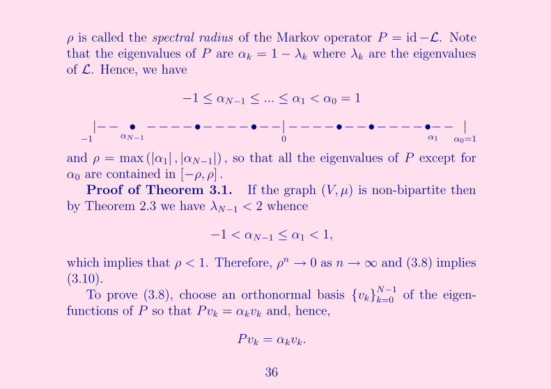
ρ is called the spectral radius of the Markov operator P = id−L. Notethat the eigenvalues of P are αk = 1 − λk where λk are the eigenvaluesof L. Hence, we have

−1 ≤ αN−1 ≤ ... ≤ α1 < α0 = 1

|−−1

− •αN−1

−−−−•−−−−•−−|0

−−−−•−−•−−−−•−α1

− |α0=1

and ρ = max (|α1| , |αN−1|) , so that all the eigenvalues of P except forα0 are contained in [−ρ, ρ] .

Proof of Theorem 3.1. If the graph (V, μ) is non-bipartite thenby Theorem 2.3 we have λN−1 < 2 whence

−1 < αN−1 ≤ α1 < 1,

which implies that ρ < 1. Therefore, ρn → 0 as n → ∞ and (3.8) implies(3.10).

To prove (3.8), choose an orthonormal basis {vk}N−1k=0 of the eigen-

functions of P so that Pvk = αkvk and, hence,

Pvk = αkvk.

36

Any function f ∈ F can be expanded in the basis vk as follows:

f =N−1∑

k=0

ckvk

where ck = (f, vk) . By the Parseval identity, we have

‖f‖2 =N−1∑

k=0

c2k.

We have

Pf =N−1∑

k=0

ckPvk =N−1∑

k=0

αkckvk,

whence, by induction in n,

P nf =N−1∑

k=0

αkckvk.

37

On the other hand, recall that v0 ≡ c for some constant c. It can bedetermined from the normalization condition ‖v0‖ = 1, that is,

∑

x∈V

c2μ (x) = 1

whence c = 1√μ(V )

. It follows that

c0 = (f, v0) =1

√μ (V )

∑

x∈V

f (x) μ (x)

and

c0v0 =1

μ (V )

∑

x∈V

f (x) μ (x) = f.

38

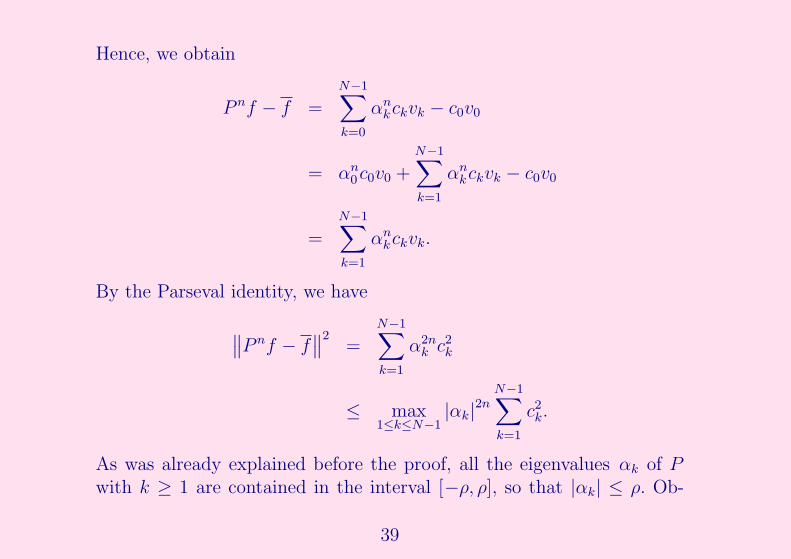
Hence, we obtain

P nf − f =N−1∑

k=0

αnkckvk − c0v0

= αn0c0v0 +

N−1∑

k=1

αnkckvk − c0v0

=N−1∑

k=1

αnkckvk.

By the Parseval identity, we have

∥∥P nf − f

∥∥2

=N−1∑

k=1

α2nk c2

k

≤ max1≤k≤N−1

|αk|2n

N−1∑

k=1

c2k.

As was already explained before the proof, all the eigenvalues αk of Pwith k ≥ 1 are contained in the interval [−ρ, ρ], so that |αk| ≤ ρ. Ob-

39

serving also thatN−1∑

k=1

c2k ≤ ‖f‖2 ,

we obtain ∥∥P nf − f

∥∥2

≤ ρ2n ‖f‖2 ,

which finishes the proof.Let us show that if λN−1 = 2 then (3.10) is not the case (as we will

see later, for bipartite graphs one has exactly λN−1 = 2). Indeed, if f isan eigenfunction of L with the eigenvalue 2 then f is the eigenfunctionof P with the eigenvalue −1, that is, Pf = −f . Then we obtain thatP nf = (−1)n f so that P nf does not converge to any function as n → ∞.

Corollary 3.2 Let (V, μ) be a finite, connected, weighted graph that isnon-bipartite, and let {Xn} be the associated random walk. Fix a vertexx0 ∈ V and consider the distribution function of Xn:

vn (x) = Px0 (Xn = x) .

40

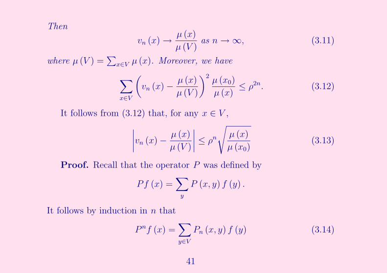
Then

vn (x) →μ (x)

μ (V )as n → ∞, (3.11)

where μ (V ) =∑

x∈V μ (x). Moreover, we have

∑

x∈V

(

vn (x) −μ (x)

μ (V )

)2μ (x0)

μ (x)≤ ρ2n. (3.12)

It follows from (3.12) that, for any x ∈ V ,

∣∣∣∣vn (x) −

μ (x)

μ (V )

∣∣∣∣ ≤ ρn

√μ (x)

μ (x0)(3.13)

Proof. Recall that the operator P was defined by

Pf (x) =∑

y

P (x, y) f (y) .

It follows by induction in n that

P nf (x) =∑

y∈V

Pn (x, y) f (y) (3.14)

41

where Pn (x, y) is the n-step transition function. Since the graph is notbipartite, we have ρ ∈ (0, 1), so that (3.11) follows from (3.12) (or from(3.13)). To prove (3.12), consider also the backward distribution function

un (x) = Px (Xn = x0) =vn (x) μ (x0)

μ (x)

(cf. (1.11)). Since

un (x) = Pn (x, x0) =∑

y∈V

Pn (x, y) 1{x0} (y) = P n1{x0} (x) ,

we obtain by Theorem 3.1 with f = 1{x0} that∥∥un − f

∥∥2

≤ ρ2n∥∥1{x0}

∥∥2

.

Since for this function f

f =1

μ (V )μ (x0) and ‖f‖2 = μ (x0) ,

we obtain that

∑

x

(vn (x) μ (x0)

μ (x)−

μ (x0)

μ (V )

)2

μ (x) ≤ ρ2nμ (x0)

42

whence (3.11) follows.A random walk is called ergodic if (3.11) is satisfied. We have seen

that a random walk on a finite, connected, non-bipartite graph is ergodic.Given a small number ε > 0, define the mixing time T = T (ε) by thecondition ρT = ε, that is

T =ln 1

ε

ln 1ρ

. (3.15)

Then, for any n ≥ T , we obtain from (3.13) that

∣∣∣∣vn (x) −

μ (x)

μ (V )

∣∣∣∣ ≤ ε

√μ (x)

μ (x0).

To ensure a good approximation vn (x) ≈ μ(x)μ(V )

, the value of ε should bechosen so that

ε

√μ (x)

μ (x0)<<

μ (x)

μ (V ),

which is equivalent to

ε << minxμ(x)μ(V )

.

43

In many examples of graphs, λ1 is close to 0 and λN−1 is close to 2.In this case, we have

ln1

|α1|= ln

1

1 − λ1

≈ λ1

and

ln1

|αN−1|= ln

1

|1 − λN−1|= ln

1

1 − (2 − λN−1)≈ 2 − λN−1,

whence

T =ln 1

ε

ln 1ρ

≈ ln1

εmax

(1

λ1

,1

2 − λN−1

)

. (3.16)

In the next sections, we will estimate the eigenvalues on specific graphsand, consequently, provide some explicit values for the mixing time.

4 Eigenvalues of bipartite graphs

The next statement contains an additional information about the spec-trum of L in some specific cases.

44

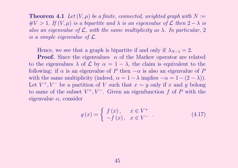
Theorem 4.1 Let (V, μ) be a finite, connected, weighted graph with N :=#V > 1. If (V, μ) is a bipartite and λ is an eigenvalue of L then 2− λ isalso an eigenvalue of L, with the same multiplicity as λ. In particular, 2is a simple eigenvalue of L.

Hence, we see that a graph is bipartite if and only if λN−1 = 2.Proof. Since the eigenvalues α of the Markov operator are related

to the eigenvalues λ of L by α = 1 − λ, the claim is equivalent to thefollowing: if α is an eigenvalue of P then −α is also an eigenvalue of Pwith the same multiplicity (indeed, α = 1−λ implies −α = 1− (2 − λ)).Let V +, V − be a partition of V such that x ∼ y only if x and y belongto same of the subset V +, V −. Given an eigenfunction f of P with theeigenvalue α, consider

g (x) =

{f (x) , x ∈ V +

−f (x) , x ∈ V − . (4.17)

45

Let us show that g is an eigenfunction of P with the eigenvalue −α. Forall x ∈ V +, we have

Pg (x) =∑

y∈V

P (x, y) g (y) =∑

y∈V −

P (x, y) g (y)

= −∑

y∈V −

P (x, y) f (y)

= −Pf (x) = −αf (x) = −αg (x) ,

and for x ∈ V − we obtain in the same way

Pg (x) =∑

y∈V +

P (x, y) g (y)

=∑

y∈V +

P (x, y) f (y) = Pf (x) = αf (x) = −αg (x) .

Hence, −α is an eigenvalue of P with the eigenfunction g.Let m be the multiplicity of α as an eigenvalue of P , and m′ be the

multiplicity of −α. Let us prove that m′ = m. There exist m linearlyindependent eigenfunctions f1, ..., fm of the eigenvalue α. Using (4.17),

46

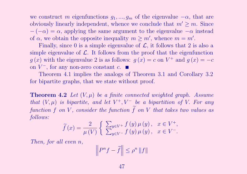
we construct m eigenfunctions g1, ..., gm of the eigenvalue −α, that areobviously linearly independent, whence we conclude that m′ ≥ m. Since− (−α) = α, applying the same argument to the eigenvalue −α insteadof α, we obtain the opposite inequality m ≥ m′, whence m = m′.

Finally, since 0 is a simple eigenvalue of L, it follows that 2 is also asimple eigenvalue of L. It follows from the proof that the eigenfunctiong (x) with the eigenvalue 2 is as follows: g (x) = c on V + and g (x) = −con V −, for any non-zero constant c.

Theorem 4.1 implies the analogs of Theorem 3.1 and Corollary 3.2for bipartite graphs, that we state without proof.

Theorem 4.2 Let (V, μ) be a finite connected weighted graph. Assumethat (V, μ) is bipartite, and let V +, V − be a bipartition of V. For any

function f on V , consider the function f on V that takes two values asfollows:

f (x) =2

μ (V )

{ ∑y∈V + f (y) μ (y) , x ∈ V +,∑y∈V − f (y) μ (y) , x ∈ V −.

Then, for all even n, ∥∥∥P nf − f

∥∥∥ ≤ ρn ‖f‖

47

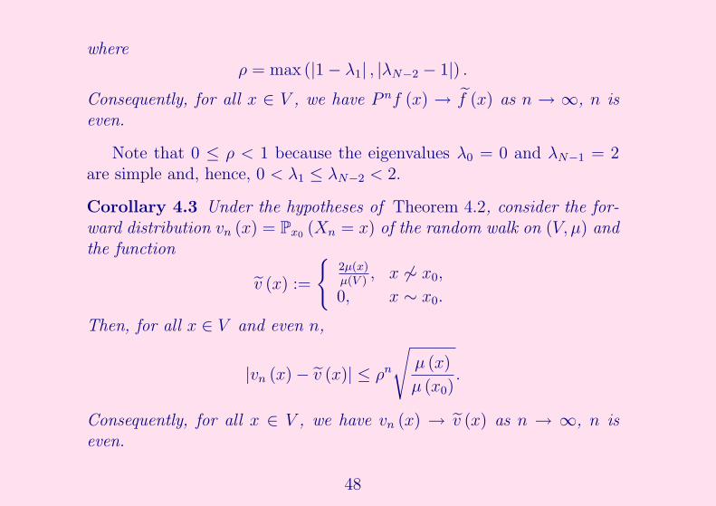
whereρ = max (|1 − λ1| , |λN−2 − 1|) .

Consequently, for all x ∈ V , we have P nf (x) → f (x) as n → ∞, n iseven.

Note that 0 ≤ ρ < 1 because the eigenvalues λ0 = 0 and λN−1 = 2are simple and, hence, 0 < λ1 ≤ λN−2 < 2.

Corollary 4.3 Under the hypotheses of Theorem 4.2, consider the for-ward distribution vn (x) = Px0 (Xn = x) of the random walk on (V, μ) andthe function

v (x) :=

{2μ(x)μ(V )

, x 6∼ x0,

0, x ∼ x0.

Then, for all x ∈ V and even n,

|vn (x) − v (x)| ≤ ρn

√μ (x)

μ (x0).

Consequently, for all x ∈ V , we have vn (x) → v (x) as n → ∞, n iseven.

48

It follows from Theorem 4.1 λ1 ≤ 1 and λN−2 = 2−λ1 so that in factρ = 1 − λ1. It follows that the mixing time (assuming that n is even) isestimated by

T =ln 1

ε

ln 1ρ

≈ln 1

ε

λ1

assuming λ1 ≈ 0. Here ε must be chosen so that ε << minxμ(x)μ(V )

.

5 Eigenvalues of Zm

Let us compute the eigenvalues of the Markov operator on the cyclegraph Zm with simple weight. Recall that Zm = {0, 1, ...,m − 1} and theconnections are

0 ∼ 1 ∼ 2 ∼ ... ∼ m − 1 ∼ 0.

The Markov operator is given by

Pf (k) =1

2(f (k + 1) + f (k − 1))

49

where k is regarded as a residue mod m. The eigenfunction equationPf = αf becomes

f (k + 1) − 2αf (k) + f (k − 1) = 0. (5.18)

We know already that α = 1 is always a simple eigenvalue of P , andα = −1 is a (simple) eigenvalue if and only if Zm is bipartite, that is, ifm is even. Assume in what follows that α ∈ (−1, 1) .

Consider first the difference equation (5.18) on Z, that is, for all k ∈ Z,and find all solutions f as functions on Z. Observe first that the set ofall solutions of (5.18) is a linear space (the sum of two solutions is asolution, and a multiple of a solution is a solution), and the dimension ofthis space is 2, because function f is uniquely determined by (5.18) andby two initial conditions f (0) = a and f (1) = b. Therefore, to find allsolutions of (5.18), it suffices to find two linearly independent solutions.

Let us search specific solution of (5.18) in the form f (k) = rk wherethe number r is to be found. Substituting into (5.18) and cancelling byrk, we obtain the equation for r:

r2 − 2αr + 1 = 0.

50

It has two complex roots

r = α ± i√

1 − α2 = e±iθ,

where θ ∈ (0, π) is determined by the condition

cos θ = α (and sin θ =√

1 − α2).

Hence, we obtain two independent complex-valued solutions of (5.18)

f1 (k) = eikθ and f2 (k) = e−ikθ.

Taking their linear combinations and using the Euler formula, we arriveat the following real-valued independent solutions:

f1 (k) = cos kθ and f2 (k) = sin kθ. (5.19)

In order to be able to consider a function f (k) on Z as a function on Zm,it must be m-periodic, that is,

f (k + m) = f (k) for all k ∈ Z.

51

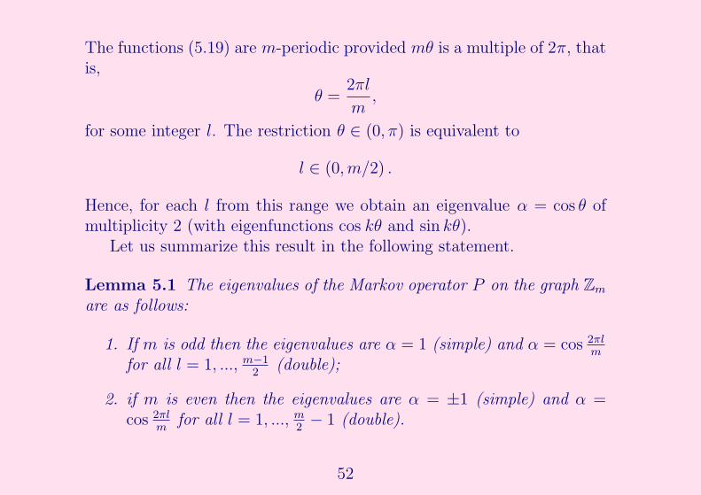
The functions (5.19) are m-periodic provided mθ is a multiple of 2π, thatis,

θ =2πl

m,

for some integer l. The restriction θ ∈ (0, π) is equivalent to

l ∈ (0,m/2) .

Hence, for each l from this range we obtain an eigenvalue α = cos θ ofmultiplicity 2 (with eigenfunctions cos kθ and sin kθ).

Let us summarize this result in the following statement.

Lemma 5.1 The eigenvalues of the Markov operator P on the graph Zm

are as follows:

1. If m is odd then the eigenvalues are α = 1 (simple) and α = cos 2πlm

for all l = 1, ..., m−12

(double);

2. if m is even then the eigenvalues are α = ±1 (simple) and α =cos 2πl

mfor all l = 1, ..., m

2− 1 (double).

52

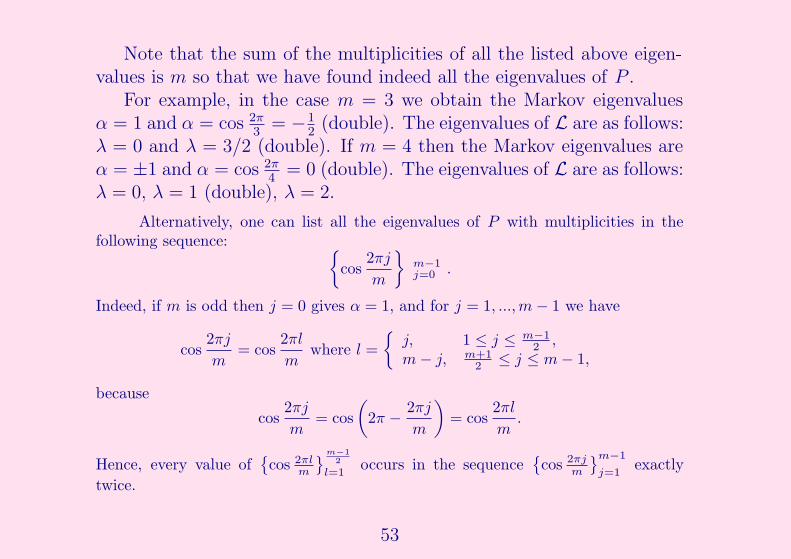
Note that the sum of the multiplicities of all the listed above eigen-values is m so that we have found indeed all the eigenvalues of P .

For example, in the case m = 3 we obtain the Markov eigenvaluesα = 1 and α = cos 2π

3= −1

2(double). The eigenvalues of L are as follows:

λ = 0 and λ = 3/2 (double). If m = 4 then the Markov eigenvalues areα = ±1 and α = cos 2π

4= 0 (double). The eigenvalues of L are as follows:

λ = 0, λ = 1 (double), λ = 2.

Alternatively, one can list all the eigenvalues of P with multiplicities in thefollowing sequence: {

cos2πj

m

}m−1j=0 .

Indeed, if m is odd then j = 0 gives α = 1, and for j = 1, ...,m − 1 we have

cos2πj

m= cos

2πl

mwhere l =

{j, 1 ≤ j ≤ m−1

2 ,m − j, m+1

2 ≤ j ≤ m − 1,

because

cos2πj

m= cos

(

2π −2πj

m

)

= cos2πl

m.

Hence, every value of{cos 2πl

m

}m−12

l=1occurs in the sequence

{cos 2πj

m

}m−1

j=1exactly

twice.

53

In the same way, if m is even, then j = 0 and j = m/2 give the values 1 and −1,respectively, while for j ∈ [1,m − 1] \ {m/2} we have

cos2πj

m= cos

2πl

mwhere l =

{j, 1 ≤ j ≤ m

2 − 1,m − j, m

2 + 1 ≤ j ≤ m − 1,

so that each value of{cos 2πl

m

}m2 −1

l=1is counted exactly twice.

6 Products of weighted graphs

Definition. Let (X, a) and (Y, b) be two finite weighted graphs. Fix twonumbers p, q > 0 and define the product graph

(V, μ) = (X, a)�p,q (Y, b)

as follows: V = X × Y and the weight μ on V is defined by

μ(x,y),(x′,y) = pb (y) axx′

μ(x,y),(x,y′) = qa (x) byy′

54

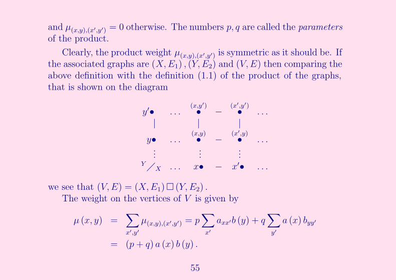
and μ(x,y),(x′,y′) = 0 otherwise. The numbers p, q are called the parametersof the product.

Clearly, the product weight μ(x,y),(x′,y′) is symmetric as it should be. Ifthe associated graphs are (X,E1) , (Y,E2) and (V,E) then comparing theabove definition with the definition (1.1) of the product of the graphs,that is shown on the diagram

y′• . . .(x,y′)• −

(x′,y′)• . . .

| | |

y• . . .(x,y)• −

(x′,y)• . . .

......

...Y�X . . . x• − x′• . . .

we see that (V,E) = (X,E1)� (Y,E2) .The weight on the vertices of V is given by

μ (x, y) =∑

x′,y′

μ(x,y),(x′,y′) = p∑

x′

axx′b (y) + q∑

y′

a (x) byy′

= (p + q) a (x) b (y) .

55

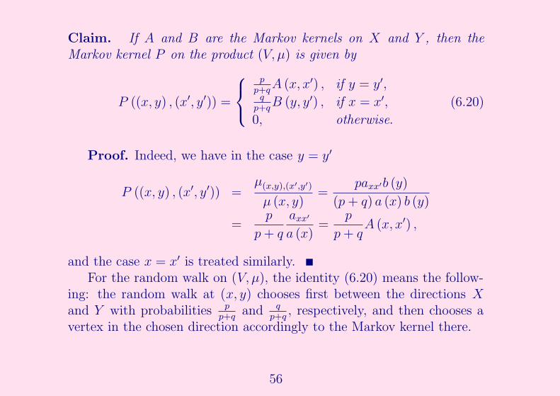
Claim. If A and B are the Markov kernels on X and Y , then theMarkov kernel P on the product (V, μ) is given by

P ((x, y) , (x′, y′)) =

pp+q

A (x, x′) , if y = y′,q

p+qB (y, y′) , if x = x′,

0, otherwise.

(6.20)

Proof. Indeed, we have in the case y = y′

P ((x, y) , (x′, y′)) =μ(x,y),(x′,y′)

μ (x, y)=

paxx′b (y)

(p + q) a (x) b (y)

=p

p + q

axx′

a (x)=

p

p + qA (x, x′) ,

and the case x = x′ is treated similarly.For the random walk on (V, μ), the identity (6.20) means the follow-

ing: the random walk at (x, y) chooses first between the directions Xand Y with probabilities p

p+qand q

p+q, respectively, and then chooses a

vertex in the chosen direction accordingly to the Markov kernel there.

56

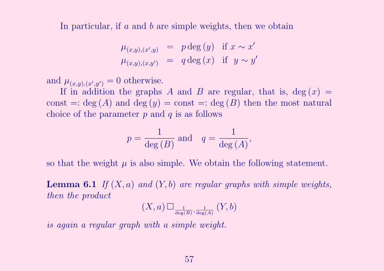
In particular, if a and b are simple weights, then we obtain

μ(x,y),(x′,y) = p deg (y) if x ∼ x′

μ(x,y),(x,y′) = q deg (x) if y ∼ y′

and μ(x,y),(x′,y′) = 0 otherwise.If in addition the graphs A and B are regular, that is, deg (x) =

const =: deg (A) and deg (y) = const =: deg (B) then the most naturalchoice of the parameter p and q is as follows

p =1

deg (B)and q =

1

deg (A),

so that the weight μ is also simple. We obtain the following statement.

Lemma 6.1 If (X, a) and (Y, b) are regular graphs with simple weights,then the product

(X, a)� 1deg(B)

, 1deg(A)

(Y, b)

is again a regular graph with a simple weight.

57

Note that the degree of the product graph is deg (A) + deg (B).

Example. Consider the graphs Znm and Zk

m with simple weights. Sincetheir degrees are equal to 2n and 2k, respectively, we obtain

Znm� 1

2k, 12nZk

m = Zn+km .

Theorem 6.2 Let (X, a) and (Y, b) be finite weighted graphs withoutisolated vertices, and let {αk}

n−1k=0 and {βl}

m−1l=0 be the sequences of the

eigenvalues of the Markov operators A and B respectively, counted withmultiplicities. Then all the eigenvalues of the Markov operator P on the

product (V, μ) = (X, a)�p,q (Y, b) are given by the sequence{

pαk+qβl

p+q

}

where k = 0, ..., n − 1 and l = 0, ...,m − 1.

In other words, the eigenvalues of P are the convex combinations ofeigenvalues of A and B, with the coefficients p

p+qand q

p+q. Note that the

same relation holds for the eigenvalues of the Laplace operators: since

58

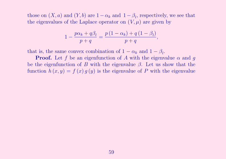
those on (X, a) and (Y, b) are 1−αk and 1−βl, respectively, we see thatthe eigenvalues of the Laplace operator on (V, μ) are given by

1 −pαk + qβl

p + q=

p (1 − αk) + q (1 − βl)

p + q,

that is, the same convex combination of 1 − αk and 1 − βl.Proof. Let f be an eigenfunction of A with the eigenvalue α and g

be the eigenfunction of B with the eigenvalue β. Let us show that thefunction h (x, y) = f (x) g (y) is the eigenvalue of P with the eigenvalue

59

pα+qβp+q

. We have

Ph (x, y) =∑

x′,y′

P ((x, y) , (x′, y′)) h (x′, y′)

=∑

x′

P ((x, y) , (x′, y)) h (x′, y) +∑

y′

P ((x, y) , (x, y′)) h (x, y′)

=p

p + q

∑

x′

A (x, x′) f (x′) g (y) +q

p + q

∑

y′

B (y, y′) f (x) g (y′)

=p

p + qAf (x) g (y) +

q

p + qf (x) Bg (y)

=p

p + qαf (x) g (y) +

q

p + qβf (x) g (y)

=pα + qβ

p + qh (x, y) ,

which was to be proved.Let {fk} be a basis in the space of functions on X such that Afk =

αkfk, and {gl} be a basis in the space of functions on Y , such that Bgl =βlgl. Then hkl (x, y) = fk (x) gl (y) is a linearly independent sequenceof functions on V = X × Y . Since the number of such functions is

60

nm = #V , we see that {hkl} is a basis in the space of functions on V .Since hkl is the eigenfunction with the eigenvalue pαk+qβl

p+q, we conclude

that the sequence pαk+qβl

p+qexhausts all the eigenvalues of P .

Corollary 6.3 Let (V,E) be a finite connected regular graph with N > 1

vertices, and set (V n, En) = (V,E)�n . Let μ be a simple weight on V ,and {αk}

N−1k=0 be the sequence of the eigenvalues of the Markov operator

on (V, μ), counted with multiplicity. Let μn be a simple weight on V n.Then the eigenvalues of the Markov operator on (V n, μn) are given by thesequence {

αk1 + αk2 + ... + αkn

n

}

(6.21)

for all ki ∈ {0, 1, ..., N − 1} , where each eigenvalue is counted with mul-tiplicity.

It follows that if {λk}N−1k=0 is the sequence of the eigenvalues of the

Laplace operator on (V, μ) then the eigenvalues of Laplace operator on(V n, μn) are given by the sequence

{λk1 + λk2 + ... + λkn

n

}

. (6.22)

61

Proof. Induction in n. If n = 1 then there is nothing to prove. Letus make the inductive step from n to n + 1. Let degree of (V,E) be D,then deg (V n) = nD. Note that.

(V n+1, En+1

)= (V n, En)� (V,E)

It follows from Lemma 6.1 that(V n+1, μn+1

)= (V n, μn)� 1

D, 1nD

(V, μ) .

By the inductive hypothesis, the eigenvalues of the Laplacian on (V n, μn)are given by the sequence (6.21). Hence, by Theorem 6.2, the eigenvalueson(V n+1, μn+1

)are given by

1/D

1/D + 1/ (nD)

αk1 + αk2 + ... + αkn

n+

1/ (nD)

1/D + 1/ (nD)αk

=n

n + 1

αk1 + αk2 + ... + αkn

n+

1

n + 1αk

=αk1 + αk2 + ... + αkn + αk

n + 1,

which was to be proved.

62

7 Eigenvalues and mixing times in Znm

Consider Znm with an odd m so that the graph Zn

m is not bipartite. ByCorollary 3.2, the distribution of the random walk on Zn

m converges to

the equilibrium measure μ(x)μ(V )

= 1N

, where N = #V = mn, and the rateof convergence is determined by the spectral radius ρ

ρ = max (|αmin| , |αmax|) (7.23)

where αmin is the minimal eigenvalue of P and αmax is the second maximaleigenvalue of P . In the case n = 1, all the eigenvalues of P except for 1are listed in the sequence (without multiplicity):

{

cos2πl

m

}

, 1 ≤ l ≤m − 1

2.

This sequence is obviously decreasing in l, and its maximal and minimalvalues are

cos2π

mand cos

(2π

m

m − 1

2

)

= − cosπ

m,

63

respectively. For a general n, by Corollary 6.3, the eigenvalue of P havethe form

αk1 + αk2 + ... + αkn

n(7.24)

where αkiare the eigenvalues of P for n = 1. The minimal value of (7.24)

is equal to the minimal value of αk, that is

αmin = − cosπ

m.

The maximal value of (7.24) is, of course, 1 when all αki= 1, and the

second maximal value is obtained when one of αkiis equal to cos 2π

mand

the rest n − 1 values are 1. Hence, we have

αmax =n − 1 + cos 2π

m

n= 1 −

1 − cos 2πm

n. (7.25)

For example, if m = 3 then αmin = − cos π3

= −12

and

αmax = 1 −1 − cos 2π

3

n= 1 −

3

2n

64

whence

ρ = max

(1

2,

∣∣∣∣1 −

3

2n

∣∣∣∣

)

=

{12, n ≤ 3,

1 − 32n

, n ≥ 4.(7.26)

If m is large then, using the approximation cos θ ≈ 1 − θ2

2for small

θ, we obtain

αmin ≈ −

(

1 −π2

2m2

)

and αmax ≈ 1 −2π2

nm2.

Using ln 11−θ

≈ θ, we obtain

ln1

|αmin|≈

π2

2m2and ln

1

|αmax|≈

2π2

nm2.

Finally, by (3.15) and (7.23), we obtain the estimate of the mixing timein Zn

m with error ε:

T =ln 1

ε

ln 1ρ

≈ ln1

εmax

(2m2

π2,nm2

2π2

)

=ln 1

ε

2π2nm2, (7.27)

65

assuming for simplicity that n ≥ 4. Choosing ε = 1N2 (note that ε must

be � 1N

) and using N = mn, we obtain

T ≈2 ln mn

2π2nm2 =

1

π2n2m2 ln m =

1

π2

m2

ln m(ln N)2 . (7.28)

Example. In Z105 with N = 510 ≈ 106, the mixing time is T ≈ 400,

which is relatively short given the fact that the number of vertices in thisgraph is In fact, the actual mixing time is even smaller than above valueof T since the latter is an upper bound for the mixing time.

Example. Take m = 3. Using the exact value of ρ given by (7.26), andobtain that, for Zn

3 with large n and ε = 1N2 = 3−2n:

T =ln 1

ε

ln(1 − 3

2n

) ≈2 ln N

3/ (2n)=

4

3 ln 3(ln N)2 ≈ 1.2 (ln N)2 .

For example, for Z133 with N = 313 > 106 vertices, we obtain a very short

mixing time T ≈ 250.

Example. For n = 1 (7.27) slightly changes to become

T ≈ ln1

ε

2m2

π2=

4

π2m2 ln m,

66

where we have chosen ε = 1m2 . For example, in Z106 with N = m = 106

we have T ' 1012, which is huge in striking contrast with the previousgraph Z10

5 with (almost) the same number of vertices as Z106 !

Example. Let us estimate the mixing time on the binary cube Zn2 that

is a bipartite graph. The eigenvalues of the Laplace operator on Z2 areλ0 = 0 and λ1 = 2. Then the eigenvalues of the Laplace operator on Zn

2

are given by (6.22), that is, by{

λk1 + λk2 + ... + λkn

n

}

where each ki = 0 or 1. Hence, each eigenvalue of Zn2 is equal to 2j

nwhere

j ∈ [0, n] is the number of 1’s in the sequence k1, ..., kn. The multiplicityof the eigenvalue 2j

nis equal to the number of binary sequences {k1, ..., kn}

where 1 occurs exactly j times. This number is given by the binomialcoefficient

(nj

). Hence, all the eigenvalues of the Laplace operator on Zn

2

are{

2jn

}where j = 0, 1, ..., n, and the multiplicity of this eigenvalue is(

nj

).The convergence rate of the random walk on Zn

2 is determined byλ1 = 2

n. Assume that n is large and let N = 2n. Taking ε = 1

N2 = 2−2n,

67

we obtain the following estimate of the mixing time:

T ≈ln 1

ε

λ1

=2n ln 2

2/n= (ln 2) n2 =

(ln N)2

ln 2≈ 1.4 (ln N)2 .

For example, for {0, 1}20 with N = 220 ≈ 106 vertices we obtain T ≈ 280.

68

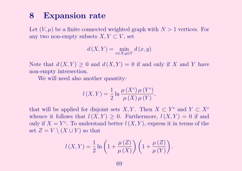
8 Expansion rate

Let (V, μ) be a finite connected weighted graph with N > 1 vertices. Forany two non-empty subsets X,Y ⊂ V , set

d (X,Y ) = minx∈X,y∈Y

d (x, y)

Note that d (X,Y ) ≥ 0 and d (X,Y ) = 0 if and only if X and Y havenon-empty intersection.

We will need also another quantity:

l (X,Y ) =1

2ln

μ (Xc) μ (Y c)

μ (X) μ (Y ),

that will be applied for disjoint sets X,Y . Then X ⊂ Y c and Y ⊂ Xc

whence it follows that l (X,Y ) ≥ 0. Furthermore, l (X,Y ) = 0 if andonly if X = Y c. To understand better l (X,Y ), express it in terms of theset Z = V \ (X ∪ Y ) so that

l (X,Y ) =1

2ln

(

1 +μ (Z)

μ (X)

)(

1 +μ (Z)

μ (Y )

)

.

69

Hence, the quantity l (X,Y ) measures the space between X and Y interms of the measure of the set Z.

Let the eigenvalues of the Laplace operator L on (V, μ) be

0 = λ0 < λ1 ≤ ... ≤ λN−1 ≤ 2.

We will use the following notation:

δ =λN−1 − λ1

λN−1 + λ1

. (8.1)

Clearly, δ ∈ [0, 1) andλ1

λN−1

=1 − δ

1 + δ.

The relation to the spectral radius

ρ = max (|1 − λ1| , |λN−1 − 1|)

is as follows: since λ1 ≥ 1 − ρ and λN−1 ≤ 1 + ρ, we obtain that

λ1

λN−1

≥1 − ρ

1 + ρ

whence δ ≤ ρ.

70

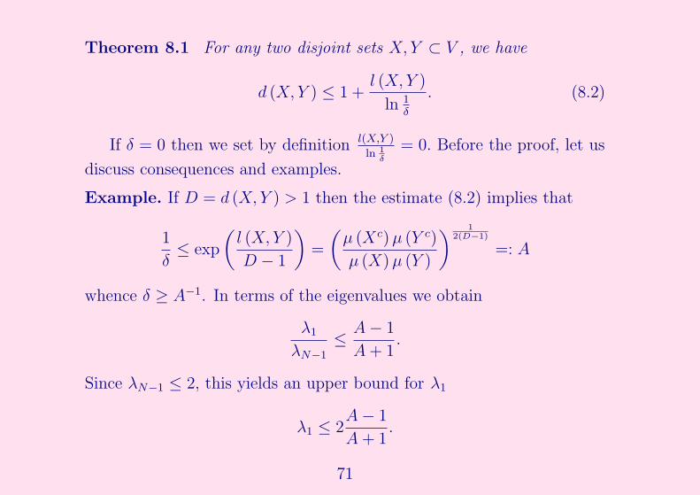
Theorem 8.1 For any two disjoint sets X,Y ⊂ V , we have

d (X,Y ) ≤ 1 +l (X,Y )

ln 1δ

. (8.2)

If δ = 0 then we set by definition l(X,Y )

ln 1δ

= 0. Before the proof, let us

discuss consequences and examples.

Example. If D = d (X,Y ) > 1 then the estimate (8.2) implies that

1

δ≤ exp

(l (X,Y )

D − 1

)

=

(μ (Xc) μ (Y c)

μ (X) μ (Y )

) 12(D−1)

=: A

whence δ ≥ A−1. In terms of the eigenvalues we obtain

λ1

λN−1

≤A − 1

A + 1.

Since λN−1 ≤ 2, this yields an upper bound for λ1

λ1 ≤ 2A − 1

A + 1.

71

Example. Let us show that

diam (V ) ≤ 1 +1

ln 1δ

lnμ (V )

m, (8.3)

where m = minx∈V μ (x). Indeed, set in (8.2) X = {x}, Y = {y} wherex, y are two distinct vertices. Then

l (X,Y ) ≤1

2ln

μ (V )2

μ (x) μ (y)≤ ln

μ (V )

m

whence

d (x, y) ≤ 1 +1

ln 1δ

lnμ (V )

m.

Taking in the left hand side the supremum in all x, y ∈ V , we obtain(8.3). In a particular case of a simple weight, we have m = minx deg (x),μ (V ) = 2#E, and

diam (V ) ≤ 1 +1

ln 1δ

ln2#E

m.

72

For any subset X ⊂ V , denote by Ur (X) the r-neighborhood of X,that is,

Ur (X) = {y ∈ V : d (y,X) ≤ r} .

Corollary 8.2 For any non-empty set X ⊂ V and any integer r ≥ 1,we have

μ (Ur (X)) ≥μ (V )

1 + μ(Xc)μ(X)

δ2r. (8.4)

Proof. Indeed, take Y = V \ Ur (X) so that Ur (X) = Y c. Thend (X,Y ) = r + 1, and (8.2) yields

r ≤1

2

1

ln 1δ

lnμ (Xc) μ (Y c)

μ (X) μ (Y ),

whenceμ (Y c)

μ (Y )≥

(1

δ

)2rμ (X)

μ (Xc).

73

Since μ (Y ) = μ (V ) − μ (Y c), we obtain

μ (V ) − μ (Y c)

μ (Y c)≤ δ2r μ (Xc)

μ (X)

whence (8.4) follows

Example. Given a set X, define the expansion rate of X to be theminimal positive integer R such that

μ (UR (X)) ≥1

2μ (V ) .

Imagine a communication network as a graph where the vertices are thecommunication centers (like computer servers) and the edges are directlinks between the centers. If X is a set of selected centers, then it isreasonable to ask, how many steps from X are required to reach themajority (at least 50%) of all centers? This is exactly the expansionrate of X, and the networks with short expansion rate provide betterconnectivity.

The inequality (8.4) implies an upper bound for the expansion rate.

74

Indeed, ifμ (Xc)

μ (X)δ2r ≤ 1, (8.5)

then (8.4) implies that μ (Ur (X)) ≥ 12μ (V ). The condition (8.5) is equiv-

alent to

r ≥1

2

ln μ(Xc)μ(X)

ln 1δ

, (8.6)

from where we see that the expansion rate R of X satisfies

R ≤1

2

ln μ(Xc)μ(X)

ln 1δ

.

Hence, a good communication network should have the number δ as smallas possible (which is similar to the requirement that ρ should be as smallas possible for a fast convergence rates to the equilibrium). For manylarge practical networks, one has the following estimate for the spectralradius: ρ ' 1

ln N(recall that λ1 and λN−1 are contained in the interval

[1 − ρ, 1 + ρ]). Since δ ≤ ρ, it follows that

1

δ& ln N.

75

Assuming that X consists of a single vertex and that μ(Xc)μ(X)

≈ N , weobtain the following estimate of the expansion rate of a single vertex:

R .ln N

ln ln N.

For example, if N = 108, which is a typical figure for the internet graph,then R ' 6 (although neglecting the constant factors). This very fastexpansion rate is called “a small world” phenomenon, and it is actuallyobserved in large communication networks.

The same phenomenon occurs in the coauthor network : two math-ematicians are connected by an edge if they have a joint publication.Although the number of recorded mathematicians is quite high (≈ 105),a few links are normally enough to get from one mathematician to asubstantial portion of the entire network.

Note for comparison that in Znm we have 1 − δ ' c

nm2 whence R .m2

ln m(ln N)2 .

Proof of Theorem 8.1. As before, denote by F the space of allreal-valued functions on V . Let w0, w1, ...., wN−1 be an orthonormal basisin F that consists of the eigenfunctions of L, and let their eigenvalues

76

be λ0 = 0, λ1, ..., λN−1. Any function u ∈ F admits an expansion in thebasis {wl} as follows:

u =

N−1∑

l=0

alwl (8.7)

with some coefficients al. We know already that

a0w0 = u =1

μ (V )

∑

x∈V

u (x) μ (x)

(see the proof of Theorem 3.1). Denote

u′ = u − u =N−1∑

l=1

alwl

so that u = u + u′ and u′⊥u.Let Φ (λ) be a polynomial with real coefficient. We have

Φ (L) u =N−1∑

l=0

alΦ (λl) wl = Φ (0) u +N−1∑

l=1

alΦ (λl) wl.

77

If v is another function from F with expansion

v =N−1∑

l=0

blwl = v +N−1∑

l=1

blwl = v + v′,

then

(Φ (L) u, v) = (Φ (0) u, v) +N−1∑

l=1

alblΦ (λl)

≥ Φ (0) uvμ (V ) − max1≤l≤N−1

|Φ (λl)|N−1∑

l=1

|al| |bl|

≥ Φ (0) uvμ (V ) − max1≤l≤N−1

|Φ (λl)| ‖u′‖ ‖v′‖ . (8.8)

Assume now that supp u ⊂ X, supp v ⊂ Y and that

D = d (X,Y ) ≥ 2

(if D ≤ 1 then (8.2) is trivially satisfied). Let Φ (λ) be a polynomial ofλ of degree D − 1. Let us verify that

(Φ (L) u, v) = 0. (8.9)

78

Indeed, the function Lku is supported in the k-neighborhood of supp u,whence it follows that Φ (L) u is supported in the (D − 1)-neighborhoodof X. Since UD−1 (X) is disjoint with Y , we obtain (8.9). Comparing(8.9) and (8.8), we obtain

max1≤l≤N−1

|Φ (λl)| ≥ Φ (0)uvμ (V )

‖u′‖ ‖v′‖. (8.10)

Let us take now u = 1X and v = 1Y . We have

u =μ (X)

μ (V ), ‖u‖2 =

μ (X)2

μ (V ), ‖u‖2 = μ (X) ,

whence

‖u′‖ =√‖u‖2 − ‖u‖2 =

√

μ (X) −μ (X)2

μ (V )=

√μ (X) μ (Xc)

μ (V ).

Using similar identities for v and substituting into (8.10), we obtain

max1≤l≤N−1

|Φ (λl)| ≥ Φ (0)

√μ (X) μ (Y )

μ (Xc) μ (Y c).

79

Finally, let us specify Φ (λ) as follows:

Φ (λ) =

(λ1 + λN−1

2− λ

)D−1

.

Since max |Φ (λ)| on the set λ ∈ [λ1, λN−1] is attained at λ = λ1 andλ = λN−1 and

max[λ1,λN−1]

|Φ (λ)| =

(λN−1 − λ1

2

)D−1

,

it follows from (8.18) that

(λN−1 − λ1

2

)D−1

≥

(λN−1 + λ1

2

)D−1√

μ (X) μ (Y )

μ (Xc) μ (Y c).

Rewriting this inequality in the form

exp (l (X,Y )) ≥

(1

δ

)D−1

80

and taking ln, we obtain (8.2).The next result is a generalization of Theorem 8.1. Set

δk =λN−1 − λk

λN−1 + λk

.

Theorem 8.3 Let k ∈ {1, 2, ..., N − 1} and X1, ..., Xk+1 be non-emptydisjoint subsets of V , and set

D = mini 6=j

d (Xi, Xj) .

Then

D ≤ 1 +1

ln 1δk

maxi 6=j

l (Xi, Xj) . (8.11)

Example. Define the k-diameter of the graph by

diamk (V ) = max{x1,...,xk+1}

mini 6=j

d (xi, xj) .

81

In particular, diam1 is the usual diameter of the graph. Applying Theo-rem 8.3 to sets Xi = {xi} and maximizing over all xi, we obtain

diamk (V ) ≤ 1 +ln μ(V )

m

ln 1δk

, (8.12)

where m = infx∈V μ (x) .

We precede the proof of Theorem 8.3 by a lemma.

Lemma 8.4 In any sequence of n+2 vectors in n-dimensional Euclideanspace, there are two vectors with non-negative inner product.

Note that n + 2 is the smallest number for which the statement ofLemma 8.4 is true. Indeed, if e1, e2, ..., en denote an orthonormal basisin the given space, let us set v := −e1 − e2 − ... − en. Then any two ofthe following n + 1 vectors

e1 + εv, e2 + εv, ...., en + εv, v

have a negative inner product, provided ε > 0 is small enough.

82

v2

v1

vn+2

v3

E

v1

v2 v3

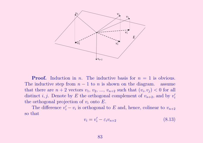
Proof. Induction in n. The inductive basis for n = 1 is obvious.The inductive step from n − 1 to n is shown on the diagram. assumethat there are n + 2 vectors v1, v2, ..., vn+2 such that (vi, vj) < 0 for alldistinct i, j. Denote by E the orthogonal complement of vn+2, and by v′

i

the orthogonal projection of vi onto E.The difference v′

i − vi is orthogonal to E and, hence, colinear to vn+2

so thatvi = v′

i − εivn+2 (8.13)

83

for some constant εi > 0. It follows, for all distinct i, j = 1, ..., n + 1,

(vi, vj) =(v′

i, v′j

)+ εiεj (vn+2, vn+2) . (8.14)

By the inductive hypothesis, in a sequence of n + 1 vectors v′1, ..., v

′n+1 in

(n − 1)-dimensional Euclidean space E, there are two vectors with non-negative inner product, say,

(v′

i, v′j

)≥ 0. It follows from (8.14) that also

(vi, vj) ≥ 0, which finishes the proof.Proof of Theorem 8.3. We use the same notation as in the proof

of Theorem 8.1. If D ≤ 1 then (8.11) is trivially satisfied. Assume in thesequel that D ≥ 2. Let ui be a function on V with supp ui ⊂ Xi. LetΦ (λ) be a polynomial with real coefficients of degree ≤ D − 1, which isnon-negative for λ ∈ {λ1, ..., λk−1} . Let us prove the following estimate

maxk≤l≤N−1

|Φ (λl)| ≥ Φ (0) mini 6=j

uiujμ (V )

‖u′i‖‖u

′j‖

. (8.15)

Expand a function ui in the basis {wl} as follows:

ui =N−1∑

l=0

a(i)l wl = ui +

k−1∑

l=1

a(i)l wl +

N−1∑

l=k

a(i)l wl.

84

It follows that

(Φ (L) ui, uj) = Φ (0) uiujμ (V ) +k−1∑

l=1

Φ (λl) a(i)l a

(j)l +

N−1∑

l=k

Φ (λl) a(i)l a

(j)l

≥ Φ (0) uiujμ (V ) +k−1∑

l=1

Φ (λl) a(i)l a

(j)l

− maxk≤l≤N−1

|Φ (λl)| ‖u′i‖∥∥u′

j

∥∥ .

Since also (Φ (L) ui, uj) = 0, it follows that

maxk≤l≤N−1

|Φ (λl)| ‖u′i‖∥∥u′

j

∥∥ ≥ Φ (0) uiujμ (V ) +

k−1∑

l=1

Φ (λl) a(i)l a

(j)l . (8.16)

In order to be able to obtain (8.15), we would like to have

k−1∑

l=1

Φ (λl) a(i)l a

(j)l ≥ 0. (8.17)

In general, (8.17) cannot be guaranteed for any couple i, j but we claimthat there exists a couple i, j of distinct indices such that (8.17) holds

85

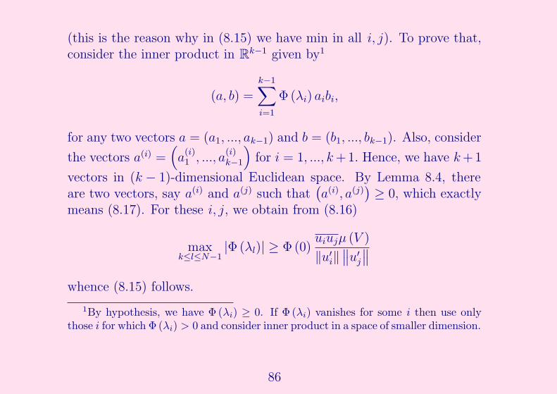
(this is the reason why in (8.15) we have min in all i, j). To prove that,consider the inner product in Rk−1 given by1

(a, b) =k−1∑

i=1

Φ (λi) aibi,

for any two vectors a = (a1, ..., ak−1) and b = (b1, ..., bk−1). Also, consider

the vectors a(i) =(a

(i)1 , ..., a

(i)k−1

)for i = 1, ..., k +1. Hence, we have k +1

vectors in (k − 1)-dimensional Euclidean space. By Lemma 8.4, thereare two vectors, say a(i) and a(j) such that

(a(i), a(j)

)≥ 0, which exactly

means (8.17). For these i, j, we obtain from (8.16)

maxk≤l≤N−1

|Φ (λl)| ≥ Φ (0)uiujμ (V )

‖u′i‖∥∥u′

j

∥∥

whence (8.15) follows.

1By hypothesis, we have Φ (λi) ≥ 0. If Φ (λi) vanishes for some i then use onlythose i for which Φ (λi) > 0 and consider inner product in a space of smaller dimension.

86

In particular, taking ui = 1Xiand using that

ui =μ (Xi)

μ (V )

and

‖u′i‖ =

√μ (Xi) μ (Xc

i )

μ (V ),

we obtain

maxk≤l≤N−1

|Φ (λl)| ≥ Φ (0) mini 6=j

√μ (Xi) μ (Xj)

μ (Xci ) μ

(Xc

j

) . (8.18)

Consider the following polynomial of degree D − 1

Φ (λ) =

(λk + λN−1

2− λ

)D−1

,

which is clearly non-negative for λ ≤ λk. Since max |Φ (λ)| on the setλ ∈ [λk, λN−1] is attained at λ = λk and λ = λN−1 and

maxλ∈[λk,λN−1]

|Φ (λ)| =

(λN−1 − λk

2

)D−1

,

87

it follows from (8.18) that

(λN−1 − λk

2

)D−1

≥

(λN−1 + λk

2

)D−1

mini 6=j

√μ (Xi) μ (Xj)

μ (Xci ) μ

(Xc

j

) ,

whence (8.11) follows.

88

9 Cheeger’s inequality

Let (V, μ) be a weighted graph with the edges set E. Recall that, for anyvertex subset Ω ⊂ V , its measure μ (Ω) is defined by

μ (Ω) =∑

x∈Ω

μ (x) .

Similarly, for any edge subset S ⊂ E, define its measure μ (S) by

μ (S) =∑

ξ∈S

μξ,

where μξ := μxy for any edge ξ = xy.For any set Ω ⊂ V , define its edge boundary ∂Ω by

∂Ω = {xy ∈ E : x ∈ Ω, y /∈ Ω} .

Definition. Given a finite weighted graph (V, μ), define its Cheegerconstant by

h = h (V, μ) = infΩ⊂V

μ(Ω)≤ 12μ(V )

μ (∂Ω)

μ (Ω). (9.19)

89

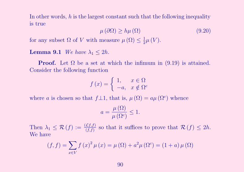
In other words, h is the largest constant such that the following inequalityis true

μ (∂Ω) ≥ hμ (Ω) (9.20)

for any subset Ω of V with measure μ (Ω) ≤ 12μ (V ).

Lemma 9.1 We have λ1 ≤ 2h.

Proof. Let Ω be a set at which the infimum in (9.19) is attained.Consider the following function

f (x) =

{1, x ∈ Ω−a, x /∈ Ωc

where a is chosen so that f⊥1, that is, μ (Ω) = aμ (Ωc) whence

a =μ (Ω)

μ (Ωc)≤ 1.

Then λ1 ≤ R (f) := (Lf,f)(f,f)

so that it suffices to prove that R (f) ≤ 2h.We have

(f, f) =∑

x∈V

f (x)2 μ (x) = μ (Ω) + a2μ (Ωc) = (1 + a) μ (Ω)

90

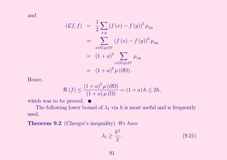
and

(Lf, f) =1

2

∑

x,y

(f (x) − f (y))2 μxy

=∑

x∈Ω,y∈Ωc

(f (x) − f (y))2 μxy

= (1 + a)2∑

x∈Ω,y∈Ωc

μxy

= (1 + a)2 μ (∂Ω) .

Hence,

R (f) ≤(1 + a)2 μ (∂Ω)

(1 + a) μ (Ω)= (1 + a) h ≤ 2h,

which was to be proved.The following lower bound of λ1 via h is most useful and is frequently

used.

Theorem 9.2 (Cheeger’s inequality) We have

λ1 ≥h2

2. (9.21)

91

Before we prove this theorem, consider some examples.

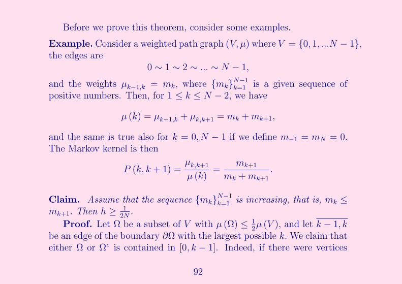
Example. Consider a weighted path graph (V, μ) where V = {0, 1, ...N − 1},the edges are

0 ∼ 1 ∼ 2 ∼ ... ∼ N − 1,

and the weights μk−1,k = mk, where {mk}N−1k=1 is a given sequence of

positive numbers. Then, for 1 ≤ k ≤ N − 2, we have

μ (k) = μk−1,k + μk,k+1 = mk + mk+1,

and the same is true also for k = 0, N − 1 if we define m−1 = mN = 0.The Markov kernel is then

P (k, k + 1) =μk,k+1

μ (k)=

mk+1

mk + mk+1

.

Claim. Assume that the sequence {mk}N−1k=1 is increasing, that is, mk ≤

mk+1. Then h ≥ 12N

.

Proof. Let Ω be a subset of V with μ (Ω) ≤ 12μ (V ), and let k − 1, k

be an edge of the boundary ∂Ω with the largest possible k. We claim thateither Ω or Ωc is contained in [0, k − 1]. Indeed, if there were vertices

92

from both sets Ω and Ωc outside [0, k−1], that is, in [k,N−1], then therewould have been an edge j − 1, j ∈ ∂Ω with j > k, which contradictsthe choice of k. It follows that either μ (Ω) ≤ μ ([0, k − 1]) or μ (Ωc) ≤μ ([0, k − 1]) . However, since μ (Ω) ≤ μ (Ωc), we obtain that in the bothcases μ (Ω) ≤ μ ([0, k − 1]) . We have

μ ([0, k − 1]) =k−1∑

j=0

μ (j) =k−1∑

j=0

(μj−1,j + μj,j+1

)

=k−1∑

j=0

(mj + mj+1)

≤ 2kmk (9.22)

where we have used that mj ≤ mj+1 ≤ mk. Therefore

μ (Ω) ≤ 2kmk.

On the other hand, we have

μ (∂Ω) ≥ μk−1,k = mk,

93

whence it follows that

μ (∂Ω)

μ (Ω)≥

mk

2kmk

=1

2k≥

1

2N,

which proves that h ≥ 12N

.Consequently, Theorem 9.2 yields

λ1 ≥1

8N2. (9.23)

For comparison, in the case of a simple weight, the exact value of λ1 is

λ1 = 1 − cosπ

N − 1

(see Exercises), which for large N is

λ1 ≈π2

2 (N − 1)2 ≈5

N 2,

which is of the same order in N as the estimate (9.23).

94

Now assume that the weights mk satisfy a stronger condition

mk+1 ≥ cmk,

for some constant c > 1 and all k = 0, ..., N − 2. Then mk ≥ ck−jmj forall k ≥ j, which allows to improve the estimate (9.22) as follows

μ ([0, k − 1]) =k−1∑

j=0

(mj + mj+1)

≤k−1∑

j=0

(cj−kmk + cj+1−kmk

)

= mk

(c−k + c1−k

) (1 + c + ...ck−1

)

= mk

(c−k + c1−k

) ck − 1

c − 1

≤ mkc + 1

c − 1.

Therefore, we obtainμ (∂Ω)

μ (Ω)≥

c − 1

c + 1

95

whence h ≥ c−1c+1

and, by Theorem 9.2,

λ1 ≥1

2

(c − 1

c + 1

)2

. (9.24)

Let us estimate the mixing time on the above path graph (V, μ). Sinceit is bipartite, the mixing time is given by

T =ln 1

ε

ln 11−λ1

≤ln 1

ε

λ1

,

where ε << minkμ(k)μ(V )

. Observe that

μ (V ) =N−1∑

j=0

(mj + mj+1) ≤ 2N−1∑

j=1

mj

where we put m0 = mN = 0, whence

mink

μ (k)

μ (V )≥

m1

2∑N−1

j=1 mj

=1

2M,

96

where

M :=

∑N−1j=1 mj

m1

.

Setting ε = 1M2 (note that M ≥ N and N can be assumed large) we

obtain

T ≤2 ln M

λ1

.

For an arbitrary increasing sequence {mk}, we obtain using (9.23) that

T ≤ 8N2 ln M.

Consider the weights mk = ck where c > 1. Then we have

M =N−1∑

j=1

cj−1 =cN−1 − 1

c − 1

whence ln M ≈ N ln c. Using also (9.24), we obtain

T ≤ 4N ln c

(c + 1

c − 1

)2

.

97

Note that T is linear in N !Consider one more example: mk = kp for some p > 1. Then

mk+1

mk

=

(

1 +1

k

)p

≥

(

1 +1

N

)p

=: c

If N >> p then c ≈ 1 + pN

whence

λ1 ≥1

2

(c − 1

c + 1

)2

≈1

8

p2

N2.

In this case,

M =N−1∑

j=1

jp ≤ Np+1,

whence ln M ≤ (p + 1) ln N and

T ≤16 (p + 1)

p2N 2 ln N.

98

We precede the proof Theorem 9.2 by two lemmas. Given a functionf : V → R and an edge ξ = xy, let us use the following notation2:

|∇ξf | := |∇xyf | = |f (y) − f (x)| .

Lemma 9.3 (Co-area formula). Given any real-valued function f on V ,set for any t ∈ R

Ωt = {x ∈ V : f(x) > t}.

Then the following identity holds:

∑

ξ∈E

|∇ξf |μξ =

∫ ∞

−∞μ(∂Ωt) dt. (9.25)

A similar formula holds for differentiable functions on R:

∫ b

a

|f ′ (x)| =

∫ ∞

−∞# {x : f (x) = t} dt,

2Note that ∇ξf is undefined unless the edge ξ is directed, whereas |∇ξf | makesalways sense.

99

and the common value of the both sides is called the full variation of f .Proof. For any edge ξ = xy, there corresponds an interval Iξ ⊂ R

that is defined as follows:

Iξ = [f(x), f(y))

where we assume that f(x) ≤ f(y) (otherwise, switch the notations xand y). Denoting by |Iξ| the Euclidean length of the interval Iξ, we seethat |∇ξf | = |Iξ| .

Claim. ξ ∈ ∂Ωt ⇔ t ∈ Iξ.Indeed, the boundary ∂Ωt consists of edges ξ = xy such that x ∈ Ωc

t

and y ∈ Ωt, that is, f(x) ≤ t and f(y) > t; which is equivalent tot ∈ [f (x) , f (y)) = Iξ.

Thus, we have

μ(∂Ωt) =∑

ξ∈∂Ωt

μξ =∑

ξ∈E:t∈Iξ

μξ =∑

ξ∈E

μξ 1Iξ(t) ,

100

whence∫ +∞

−∞μ(∂Ωt) dt =

∫ +∞

−∞

∑

ξ∈E

μξ 1Iξ(t)dt

=∑

ξ∈E

∫ +∞

−∞μξ 1Iξ

(t)dt

=∑

ξ∈E

μξ |Iξ| =∑

ξ∈E

μξ|∇ξf | ,

which finishes the proof.

Lemma 9.4 For any non-negative function f on V , such that

μ {x ∈ V : f (x) > 0} ≤1

2μ (V ) , (9.26)

the following is true:∑

ξ∈E

|∇ξf |μξ ≥ h∑

x∈V

f (x) μ (x) , (9.27)

where h is the Cheeger constant of (V, μ) .

101

Note that for the function f = 1Ω the condition (9.26) means thatμ (Ω) ≤ 1

2μ (V ), and the inequality (9.27) is equivalent to

μ (∂Ω) ≥ hμ (Ω) ,

because ∑

x∈V

f (x) μ (x) =∑

x∈Ω

μ (x) = μ (Ω)

and∑

ξ∈E

|∇ξf |μξ =∑

x∈Ω,y∈Ωc

|f (y) − f (x)|μxy =∑

x∈Ω,y∈Ωc

μxy = μ (∂Ω) .

Hence, the meaning of Lemma 9.4 is that the inequality (9.27) for theindicator functions implies the same inequality for arbitrary functions.

Proof. By the co-area formula, we have∑

ξ∈E

|∇ξf |μξ =

∫ ∞

−∞μ(∂Ωt) dt ≥

∫ ∞

0

μ(∂Ωt) dt.

By (9.26), the set Ωt = {x ∈ V : f (x) > t} has measure ≤ 12μ (V ) for

any t ≥ 0. Therefore, by (9.20)

μ (∂Ωt) ≥ hμ (Ωt)

102

whence ∑

ξ∈E

|∇ξf |μξ ≥ h

∫ ∞

0

μ (Ωt) dt

On the other hand, noticing that x ∈ Ωt for a non-negative t is equivalentto t ∈ [0, f (x)), we obtain

∫ ∞

0

μ (Ωt) dt =

∫ ∞

0

∑

x∈Ωt

μ (x) dt

=

∫ ∞

0

∑

x∈V

μ (x) 1[0,f(x)) (t) dt

=∑

x∈V

μ (x)

∫ ∞

0

1[0,f(x)) (t) dt

=∑

x∈V

μ (x) f (x) ,

which finishes the proof.Proof of Theorem 9.2. Let f be the eigenfunction of λ1. Consider

two sets

V + = {x ∈ V : f (x) ≥ 0} and V − = {x ∈ V : f (x) < 0} .

103

Without loss of generality, we can assume that μ (V +) ≤ μ (V −) (if notthen replace f by −f). It follows that μ (V +) ≤ 1

2μ (V ) . Consider the

function

g = f+ :=

{f, f ≥ 0,0, f < 0.

Applying the Green formula (2.4)

(Lf, g) =1

2

∑

x,y∈V

(∇xyf) (∇xyg) μxy

and using so that Lf = λ1f , we obtain

λ1

∑

x∈V

f(x)g(x)μ(x) =1

2

∑

x,y∈V

(∇xyf) (∇xyg) μxy.

Observing that fg = g2 and

(∇xyf) (∇xyg) = (f (y) − f (x)) (g (y) − g (x)) ≥ (g (y) − g (x))2 = |∇xyg|2 .

we obtain

λ1 ≥

∑ξ∈E |∇ξg|

2 μξ∑x∈V g2 (x) μ (x)

.

104

Note that g 6≡ 0 because otherwise f+ ≡ 0 and (f, 1) = 0 imply thatf− ≡ 0 whereas f is not identical 0.

Hence, to prove (9.21) it suffices to verify that

∑

ξ∈E

|∇ξg|2 μξ ≥

h2

2

∑

x∈V

g2 (x) μ (x) . (9.28)

Since

μ (x ∈ V : g (x) > 0) ≤ μ(V +)≤

1

2μ (V ) ,

we can apply (9.27) to function g2, which yields

∑

ξ∈E

∣∣∇ξ

(g2)∣∣μξ ≥ h

∑

x∈V

g2 (x) μ (x) . (9.29)

105

Let us estimate from above the left hand side as follows:

∑

ξ∈E

∣∣∇ξ

(g2)∣∣μξ =

1

2

∑

x,y∈V

∣∣g2(x) − g2(y)

∣∣μxy

=1

2

∑

x,y

|g(x) − g(y)|μ1/2xy |g(x) + g(y)|μ1/2

xy

≤

(1

2(∑

x,y

(g(x) − g(y))2μxy)1

2(∑

x,y

(g(x) + g(y))2μxy)

)1/2

,

where we have used the Cauchy-Schwarz inequality

∑

k

akbk ≤

(∑

k

a2k

)1/2(∑

k

b2k

)1/2

that is true for arbitrary sequences of non-negative reals ak, bk. Next,

106

using the inequality 12(a + b)2 ≤ a2 + b2, we obtain

∑

ξ∈E

∣∣∇ξ

(g2)∣∣μξ ≤

(∑

ξ∈E

|∇ξg|2 μξ

∑

x,y

(g2(x) + g2(y)

)μxy

)1/2

=

(

2∑

ξ∈E

|∇ξg|2 μξ

∑

x,y

g2(x)μxy

)1/2

=

(

2∑

ξ∈E

|∇ξg|2 μξ

∑

x∈V

g2(x)μ (x)

)1/2

,

which together with (9.29) yields

h∑

x∈V

g2 (x) μ (x) ≤

(

2∑

ξ∈E

|∇ξg|2 μξ

)1/2(∑

x∈V

g2(x)μ (x)

)1/2

.

Dividing by(∑

x∈V g2 (x) μ (x))1/2

and taking square, we obtain (9.28).

107