Embed Size (px)
Citation preview

Laplace-Beltrami:The Swiss Army Knife of Geometry Processing
(SGP 2014 Tutorial—July 7 2014)
Justin Solomon / Stanford UniversityKeenan Crane / Columbia UniversityEtienne Vouga / Harvard University

INTRODUCTION

Introduction
• Laplace-Beltrami operator (“Laplacian”) provides a basis fora diverse variety of geometry processing tasks.
• Remarkably common pipeline:1 simple pre-processing (build f )2 solve a PDE involving the Laplacian (e.g., Du = f )3 simple post-processing (do something with u)
• Expressing tasks in terms of Laplacian/smooth PDEsmakes life easier at code/implementation level.
• Lots of existing theory to help understand/interpretalgorithms, provide analysis/guarantees.
• Also makes it easy to work with a broad range ofgeometric data structures (meshes, point clouds, etc.)

Introduction
• Laplace-Beltrami operator (“Laplacian”) provides a basis fora diverse variety of geometry processing tasks.
• Remarkably common pipeline:
1 simple pre-processing (build f )2 solve a PDE involving the Laplacian (e.g., Du = f )3 simple post-processing (do something with u)
• Expressing tasks in terms of Laplacian/smooth PDEsmakes life easier at code/implementation level.
• Lots of existing theory to help understand/interpretalgorithms, provide analysis/guarantees.
• Also makes it easy to work with a broad range ofgeometric data structures (meshes, point clouds, etc.)

Introduction
• Laplace-Beltrami operator (“Laplacian”) provides a basis fora diverse variety of geometry processing tasks.
• Remarkably common pipeline:1 simple pre-processing (build f )
2 solve a PDE involving the Laplacian (e.g., Du = f )3 simple post-processing (do something with u)
• Expressing tasks in terms of Laplacian/smooth PDEsmakes life easier at code/implementation level.
• Lots of existing theory to help understand/interpretalgorithms, provide analysis/guarantees.
• Also makes it easy to work with a broad range ofgeometric data structures (meshes, point clouds, etc.)

Introduction
• Laplace-Beltrami operator (“Laplacian”) provides a basis fora diverse variety of geometry processing tasks.
• Remarkably common pipeline:1 simple pre-processing (build f )2 solve a PDE involving the Laplacian (e.g., Du = f )
3 simple post-processing (do something with u)
• Expressing tasks in terms of Laplacian/smooth PDEsmakes life easier at code/implementation level.
• Lots of existing theory to help understand/interpretalgorithms, provide analysis/guarantees.
• Also makes it easy to work with a broad range ofgeometric data structures (meshes, point clouds, etc.)

Introduction
• Laplace-Beltrami operator (“Laplacian”) provides a basis fora diverse variety of geometry processing tasks.
• Remarkably common pipeline:1 simple pre-processing (build f )2 solve a PDE involving the Laplacian (e.g., Du = f )3 simple post-processing (do something with u)
• Expressing tasks in terms of Laplacian/smooth PDEsmakes life easier at code/implementation level.
• Lots of existing theory to help understand/interpretalgorithms, provide analysis/guarantees.
• Also makes it easy to work with a broad range ofgeometric data structures (meshes, point clouds, etc.)

Introduction
• Laplace-Beltrami operator (“Laplacian”) provides a basis fora diverse variety of geometry processing tasks.
• Remarkably common pipeline:1 simple pre-processing (build f )2 solve a PDE involving the Laplacian (e.g., Du = f )3 simple post-processing (do something with u)
• Expressing tasks in terms of Laplacian/smooth PDEsmakes life easier at code/implementation level.
• Lots of existing theory to help understand/interpretalgorithms, provide analysis/guarantees.
• Also makes it easy to work with a broad range ofgeometric data structures (meshes, point clouds, etc.)

Introduction
• Goals of this tutorial:
• Understand the Laplacian in the smooth setting. (Etienne)
• Build the Laplacian in the discrete setting. (Keenan)
• Use Laplacian to implement a variety of methods. (Justin)

Introduction
• Goals of this tutorial:• Understand the Laplacian in the smooth setting. (Etienne)
• Build the Laplacian in the discrete setting. (Keenan)
• Use Laplacian to implement a variety of methods. (Justin)

Introduction
• Goals of this tutorial:• Understand the Laplacian in the smooth setting. (Etienne)
• Build the Laplacian in the discrete setting. (Keenan)
• Use Laplacian to implement a variety of methods. (Justin)

Introduction
• Goals of this tutorial:• Understand the Laplacian in the smooth setting. (Etienne)
• Build the Laplacian in the discrete setting. (Keenan)
• Use Laplacian to implement a variety of methods. (Justin)

SMOOTH THEORY

The Interpolation Problem
W
∂W
f = �1
f = 1
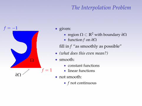
• given:• region W ⇢ R2 with boundary ∂W• function f on ∂W
fill in f “as smoothly as possible”
• (what does this even mean?)• smooth:
• constant functions• linear functions
• not smooth:• f not continuous• large variations over short distances• (krfk large)

The Interpolation Problem
W
∂W
f = �1
f = 1
• given:• region W ⇢ R2 with boundary ∂W• function f on ∂W
fill in f “as smoothly as possible”• (what does this even mean?)
• smooth:• constant functions• linear functions
• not smooth:• f not continuous• large variations over short distances• (krfk large)

The Interpolation Problem
W
∂W
f = �1
f = 1
• given:• region W ⇢ R2 with boundary ∂W• function f on ∂W
fill in f “as smoothly as possible”• (what does this even mean?)• smooth:
• constant functions• linear functions
• not smooth:• f not continuous• large variations over short distances• (krfk large)
The Interpolation Problem
W
∂W
f = �1
f = 1
• given:• region W ⇢ R2 with boundary ∂W• function f on ∂W
fill in f “as smoothly as possible”• (what does this even mean?)• smooth:
• constant functions• linear functions
• not smooth:• f not continuous
• large variations over short distances• (krfk large)

The Interpolation Problem
W
∂W
f = �1
f = 1
• given:• region W ⇢ R2 with boundary ∂W• function f on ∂W
fill in f “as smoothly as possible”• (what does this even mean?)• smooth:
• constant functions• linear functions
• not smooth:• f not continuous• large variations over short distances• (krfk large)

Dirichlet Energy
non-smooth f (x)
krfk2
• E(f ) =R
W krfk2 dA• properties:
• nonnegative• zero for constant functions• measures smoothness
• solution to interpolation problem isminimizer of E
• how do we find minimum?

Dirichlet Energy
non-smooth f (x)
krfk2
• E(f ) =R
W krfk2 dA• properties:
• nonnegative• zero for constant functions• measures smoothness
• solution to interpolation problem isminimizer of E
• how do we find minimum?

Dirichlet Energy
non-smooth f (x)
krfk2
• E(f ) =R
W krfk2 dA• properties:
• nonnegative• zero for constant functions• measures smoothness
• solution to interpolation problem isminimizer of E
• how do we find minimum?

Dirichlet Energy
non-smooth f (x)
krfk2
• E(f ) =R
W krfk2 dA• it can be shown that:
• E(f ) = C�R
W f Df dA
• �2Df is the gradient of Dirichlet energy• f minimizes E if Df = 0
• PDE form (Laplace’s Equation):
Df (x) = 0 x 2 W
f (x) = f0(x) x 2 ∂W
• physical interpretation: temperature atsteady state

Dirichlet Energy
non-smooth f (x)
Df
• E(f ) =R
W krfk2 dA• it can be shown that:
• E(f ) = C�R
W f Df dA• �2Df is the gradient of Dirichlet energy
• f minimizes E if Df = 0
• PDE form (Laplace’s Equation):
Df (x) = 0 x 2 W
f (x) = f0(x) x 2 ∂W
• physical interpretation: temperature atsteady state

Dirichlet Energy
non-smooth f (x)
Df
• E(f ) =R
W krfk2 dA• it can be shown that:
• E(f ) = C�R
W f Df dA• �2Df is the gradient of Dirichlet energy• f minimizes E if Df = 0
• PDE form (Laplace’s Equation):
Df (x) = 0 x 2 W
f (x) = f0(x) x 2 ∂W
• physical interpretation: temperature atsteady state

Dirichlet Energy
non-smooth f (x)
solution Df = 0
• E(f ) =R
W krfk2 dA• it can be shown that:
• E(f ) = C�R
W f Df dA• �2Df is the gradient of Dirichlet energy• f minimizes E if Df = 0
• PDE form (Laplace’s Equation):
Df (x) = 0 x 2 W
f (x) = f0(x) x 2 ∂W
• physical interpretation: temperature atsteady state

On a Surfacef = �1
f = 1
boundary conditions nonsmooth f (x)
• can still define Dirichlet energy E(f ) =R
M krfk2
• rE(f ) = �Df , now D is the Laplace-Beltrami operator of M• also works in higher dimensions, on discrete graphs/point
clouds, . . .

On a Surfacef = �1
f = 1
boundary conditions nonsmooth f (x) krfk2
• can still define Dirichlet energy E(f ) =R
M krfk2
• rE(f ) = �Df , now D is the Laplace-Beltrami operator of M• also works in higher dimensions, on discrete graphs/point
clouds, . . .

On a Surfacef = �1
f = 1
boundary conditions nonsmooth f (x) Df = 0
• can still define Dirichlet energy E(f ) =R
M krfk2
• rE(f ) = �Df , now D is the Laplace-Beltrami operator of M
• also works in higher dimensions, on discrete graphs/pointclouds, . . .

On a Surfacef = �1
f = 1
boundary conditions nonsmooth f (x) Df = 0
• can still define Dirichlet energy E(f ) =R
M krfk2
• rE(f ) = �Df , now D is the Laplace-Beltrami operator of M• also works in higher dimensions, on discrete graphs/point
clouds, . . .

Existence and Uniqueness
• Laplace’s equation
Df (x) = 0 x 2 M
f (x) = f0(x) x 2 ∂M
has a unique solution for all reasonable1 surfaces M
1e.g. compact, smooth, with piecewise smooth boundary

Existence and Uniqueness
• Laplace’s equation
Df (x) = 0 x 2 M
f (x) = f0(x) x 2 ∂M
has a unique solution for all reasonable1 surfaces M
• physical interpretation: apply heating/cooling f0 to theboundary of a metal plate. Interior temperature will reachsome steady state
• gradient descent is exactly the heat or diffusion equation
dfdt(x) = Df (x).
1e.g. compact, smooth, with piecewise smooth boundary
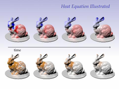
Heat Equation Illustrated
time

Boundary Conditions
W
∂WD
∂WN
g0 = 0
f0 = �1
f0 = 1
• can specify rf · n on boundary insteadof f :
Df (x) = 0 x 2 W
f (x) = f0(x) x 2 ∂WD (Dirichlet bdry)
rf · n = g0(x) x 2 ∂WN (Neumann bdry)
• usually: g0 = 0 (natural bdry conds)• physical interpretation: free boundary
through which heat cannot flow

Boundary Conditions
W
∂WD
∂WN
g0 = 0
f0 = �1
f0 = 1
• can specify rf · n on boundary insteadof f :
Df (x) = 0 x 2 W
f (x) = f0(x) x 2 ∂WD (Dirichlet bdry)
rf · n = g0(x) x 2 ∂WN (Neumann bdry)
• usually: g0 = 0 (natural bdry conds)
• physical interpretation: free boundarythrough which heat cannot flow

Boundary Conditions
W
∂WD
∂WN
g0 = 0
f0 = �1
f0 = 1
• can specify rf · n on boundary insteadof f :
Df (x) = 0 x 2 W
f (x) = f0(x) x 2 ∂WD (Dirichlet bdry)
rf · n = g0(x) x 2 ∂WN (Neumann bdry)
• usually: g0 = 0 (natural bdry conds)• physical interpretation: free boundary
through which heat cannot flow

Interpolation with D in Practice
in geometry processing:• positions• displacements• vector fields• parameterizations• . . . you name it
Joshi et al
Eck et al
Sorkine and Cohen-Or

Heat Equation with Sourcef = �1
g = 1
• what if you add heat sources inside W?
dfdt(x) = g(x) + Df (x)
• PDE form: Poisson’s equation
Df (x) = g(x) x 2 W
f (x) = f0(x) x 2 ∂W
• common variational problem:
minf
Z
Mkrf � vk2 dA
• becomes Poisson problem, g = r · v

Heat Equation with Sourcef = �1
g = 1
• what if you add heat sources inside W?
dfdt(x) = g(x) + Df (x)
• PDE form: Poisson’s equation
Df (x) = g(x) x 2 W
f (x) = f0(x) x 2 ∂W
• common variational problem:
minf
Z
Mkrf � vk2 dA
• becomes Poisson problem, g = r · v

Heat Equation with Sourcef = �1
g = 1
• what if you add heat sources inside W?
dfdt(x) = g(x) + Df (x)
• PDE form: Poisson’s equation
Df (x) = g(x) x 2 W
f (x) = f0(x) x 2 ∂W
• common variational problem:
minf
Z
Mkrf � vk2 dA
• becomes Poisson problem, g = r · v

Heat Equation with Sourcef = �1
g = 1
• what if you add heat sources inside W?
dfdt(x) = g(x) + Df (x)
• PDE form: Poisson’s equation
Df (x) = g(x) x 2 W
f (x) = f0(x) x 2 ∂W
• common variational problem:
minf
Z
Mkrf � vk2 dA
• becomes Poisson problem, g = r · v

Heat Equation with Sourcef = �1
g = 1
• what if you add heat sources inside W?
dfdt(x) = g(x) + Df (x)
• PDE form: Poisson’s equation
Df (x) = g(x) x 2 W
f (x) = f0(x) x 2 ∂W
• common variational problem:
minf
Z
Mkrf � vk2 dA
• becomes Poisson problem, g = r · v

Essential Algebraic Properties I
• linearity: D (f (x) + ag(x)) = Df (x) + aDg(x)
• constants in kernel: Da = 0
for functions that vanish on ∂M:
• self-adjoint:Z
Mf Dg dA = �
Z
Mhrf ,rgi dA =
Z
MgDf dA
• negative:Z
Mf Df dA 0
(intuition: D ⇡ an •-dimensional negative-semidefinite matrix)

Essential Algebraic Properties I
• linearity: D (f (x) + ag(x)) = Df (x) + aDg(x)• constants in kernel: Da = 0
for functions that vanish on ∂M:
• self-adjoint:Z
Mf Dg dA = �
Z
Mhrf ,rgi dA =
Z
MgDf dA
• negative:Z
Mf Df dA 0
(intuition: D ⇡ an •-dimensional negative-semidefinite matrix)

Essential Algebraic Properties I
• linearity: D (f (x) + ag(x)) = Df (x) + aDg(x)• constants in kernel: Da = 0
for functions that vanish on ∂M:
• self-adjoint:Z
Mf Dg dA = �
Z
Mhrf ,rgi dA =
Z
MgDf dA
• negative:Z
Mf Df dA 0
(intuition: D ⇡ an •-dimensional negative-semidefinite matrix)

Essential Algebraic Properties I
• linearity: D (f (x) + ag(x)) = Df (x) + aDg(x)• constants in kernel: Da = 0
for functions that vanish on ∂M:
• self-adjoint:Z
Mf Dg dA = �
Z
Mhrf ,rgi dA =
Z
MgDf dA
• negative:Z
Mf Df dA 0
(intuition: D ⇡ an •-dimensional negative-semidefinite matrix)

Solving Poisson’s Equation with Green’s Functions
• the Green’s function G on R2 solves Df = g for g = d
• linearity: if g = Â aid(x� xi), f = Â aiG(x� xi)
• for any g, f = G ⇤ g
d(x) G(x)

Solving Poisson’s Equation with Green’s Functions
• the Green’s function G on R2 solves Df = g for g = d
• linearity: if g = Â aid(x� xi), f = Â aiG(x� xi)
• for any g, f = G ⇤ g
d(x) G(x)

Solving Poisson’s Equation with Green’s Functions
• the Green’s function G on R2 solves Df = g for g = d
• linearity: if g = Â aid(x� xi), f = Â aiG(x� xi)
• for any g, f = G ⇤ g
d(x) G(x)

Essential Algebraic Properties IIa function f : M! R with Df = 0 is called harmonic. Properties:
• f is smooth and analytic
• f (x) is the average of f over any disk around x:
f (x) =1
pr2
Z
B(x,r)f (y) dA
some harmonic f (x, y)

Essential Algebraic Properties IIa function f : M! R with Df = 0 is called harmonic. Properties:
• f is smooth and analytic• f (x) is the average of f over any disk around x:
f (x) =1
pr2
Z
B(x,r)f (y) dA

Essential Algebraic Properties IIa function f : M! R with Df = 0 is called harmonic. Properties:
• f is smooth and analytic• f (x) is the average of f over any disk around x:
f (x) =1
pr2
Z
B(x,r)f (y) dA
• maximum principle: f has no local maxima or minima in M

Essential Algebraic Properties IIa function f : M! R with Df = 0 is called harmonic. Properties:
• f is smooth and analytic• f (x) is the average of f over any disk around x:
f (x) =1
pr2
Z
B(x,r)f (y) dA
• maximum principle: f has no local maxima or minima in M• (can have saddle points)

Essential Geometric Properties I
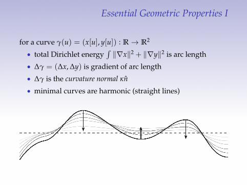
for a curve g(u) = (x[u], y[u]) : R ! R2
• total Dirichlet energyRkrxk2 + kryk2 is arc length
• Dg = (Dx, Dy) is gradient of arc length• Dg is the curvature normal kn• minimal curves are harmonic
(straight lines)

Essential Geometric Properties I
for a curve g(u) = (x[u], y[u]) : R ! R2
• total Dirichlet energyRkrxk2 + kryk2 is arc length
• Dg = (Dx, Dy) is gradient of arc length
• Dg is the curvature normal kn• minimal curves are harmonic
(straight lines)

Essential Geometric Properties I
for a curve g(u) = (x[u], y[u]) : R ! R2
• total Dirichlet energyRkrxk2 + kryk2 is arc length
• Dg = (Dx, Dy) is gradient of arc length• Dg is the curvature normal kn
• minimal curves are harmonic
(straight lines)

Essential Geometric Properties I
for a curve g(u) = (x[u], y[u]) : R ! R2
• total Dirichlet energyRkrxk2 + kryk2 is arc length
• Dg = (Dx, Dy) is gradient of arc length• Dg is the curvature normal kn• minimal curves are harmonic
(straight lines)
Essential Geometric Properties I
for a curve g(u) = (x[u], y[u]) : R ! R2
• total Dirichlet energyRkrxk2 + kryk2 is arc length
• Dg = (Dx, Dy) is gradient of arc length• Dg is the curvature normal kn• minimal curves are harmonic (straight lines)

Essential Geometric Properties II
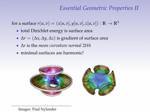
for a surface r(u, v) = (x[u, v], y[u, v], z[u, v]) : R ! R3
• total Dirichlet energy is surface area• Dr = (Dx, Dy, Dz) is gradient of surface area
• Dr is the mean curvature normal 2Hn• minimal surfaces are harmonic!

Essential Geometric Properties II
for a surface r(u, v) = (x[u, v], y[u, v], z[u, v]) : R ! R3
• total Dirichlet energy is surface area• Dr = (Dx, Dy, Dz) is gradient of surface area• Dr is the mean curvature normal 2Hn
• minimal surfaces are harmonic!
Essential Geometric Properties II
for a surface r(u, v) = (x[u, v], y[u, v], z[u, v]) : R ! R3
• total Dirichlet energy is surface area• Dr = (Dx, Dy, Dz) is gradient of surface area• Dr is the mean curvature normal 2Hn• minimal surfaces are harmonic!
Images: Paul Nylander

Essential Geometric Properties III
• D is intrinsic
• for W ⇢ R2, rigid motions of W don’t change D
• for a surface W, isometric deformations of W don’t change D

Essential Geometric Properties III
• D is intrinsic• for W ⇢ R2, rigid motions of W don’t change D
• for a surface W, isometric deformations of W don’t change D

Essential Geometric Properties III
• D is intrinsic• for W ⇢ R2, rigid motions of W don’t change D• for a surface W, isometric deformations of W don’t change D

Signal Processing on a Line
on line segment [0, 1]:• recall Fourier basis: fi(x) = cos(ix)

Signal Processing on a Line
on line segment [0, 1]:• recall Fourier basis: fi(x) = cos(ix)• can decompose f = Â aifi
• fi satisfies Dfi = �i2fi
• Dirichlet energy of f : Â i2ai
f (x) =N
Âi=1
aifi(x)| {z }
low-frequency base
+•
Âi=N+1
aifi(x)
| {z }high-frequency detail

Signal Processing on a Line
on line segment [0, 1]:• recall Fourier basis: fi(x) = cos(ix)• can decompose f = Â aifi
• fi satisfies Dfi = �i2fi
• Dirichlet energy of f : Â i2ai
f (x) =N
Âi=1
aifi(x)| {z }
low-frequency base
+•
Âi=N+1
aifi(x)
| {z }high-frequency detail

Signal Processing on a Line
on line segment [0, 1]:• recall Fourier basis: fi(x) = cos(ix)• can decompose f = Â aifi
• fi satisfies Dfi = �i2fi
• Dirichlet energy of f : Â i2ai
f (x) =N
Âi=1
aifi(x)| {z }
low-frequency base
+•
Âi=N+1
aifi(x)
| {z }high-frequency detail

Signal Processing on a Line
on line segment [0, 1]:• recall Fourier basis: fi(x) = cos(ix)• can decompose f = Â aifi
• fi satisfies Dfi = �i2fi
• Dirichlet energy of f : Â i2ai
f (x) =N
Âi=1
aifi(x)| {z }
low-frequency base
+•
Âi=N+1
aifi(x)
| {z }high-frequency detail

Laplacian Spectrum
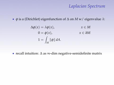
• f is a (Dirichlet) eigenfunction of D on M w/ eigenvalue l:
Df(x) = lf(x), x 2 M
0 = f(x), x 2 ∂M
1 =Z
Mkfk dA.
• recall intuition: D as •-dim negative-semidefinite matrix• expect orthogonal eigenfunctions with negative eigenvalue• spectrum is discrete: countably many eigenfunctions,
0 � l1 � l2 � l3 . . .
Laplacian Spectrum
• f is a (Dirichlet) eigenfunction of D on M w/ eigenvalue l:
Df(x) = lf(x), x 2 M
0 = f(x), x 2 ∂M
1 =Z
Mkfk dA.
• recall intuition: D as •-dim negative-semidefinite matrix
• expect orthogonal eigenfunctions with negative eigenvalue• spectrum is discrete: countably many eigenfunctions,
0 � l1 � l2 � l3 . . .

Laplacian Spectrum
• f is a (Dirichlet) eigenfunction of D on M w/ eigenvalue l:
Df(x) = lf(x), x 2 M
0 = f(x), x 2 ∂M
1 =Z
Mkfk dA.
• recall intuition: D as •-dim negative-semidefinite matrix• expect orthogonal eigenfunctions with negative eigenvalue
• spectrum is discrete: countably many eigenfunctions,
0 � l1 � l2 � l3 . . .

Laplacian Spectrum
• f is a (Dirichlet) eigenfunction of D on M w/ eigenvalue l:
Df(x) = lf(x), x 2 M
0 = f(x), x 2 ∂M
1 =Z
Mkfk dA.
• recall intuition: D as •-dim negative-semidefinite matrix• expect orthogonal eigenfunctions with negative eigenvalue• spectrum is discrete: countably many eigenfunctions,
0 � l1 � l2 � l3 . . .

Laplacian Spectrum of Bunny
f2
f6
f3
f18

Laplacian Spectrum: Signal Processing
• expand function f in eigenbasis:
f (x) = Âi
aifi(x)
• Dirichlet energy of f :
E(f ) =Z
Mkrfk2 dA = �
Z
Mf Df dA = Â
ia2
i (�li)

Laplacian Spectrum: Signal Processing
• expand function f in eigenbasis:
f (x) = Âi
aifi(x)
• Dirichlet energy of f :
E(f ) =Z
Mkrfk2 dA = �
Z
Mf Df dA = Â
ia2
i (�li)
• large li terms dominate
f (x) =N
Âi=1
aifi(x)| {z }
low-frequency base
+•
Âi=N+1
aifi(x)
| {z }high-frequency detail

Laplacian Spectrum: Signal Processing
10 modes 25 modes 50 modes
• large li terms dominate
f (x) =N
Âi=1
aifi(x)| {z }
low-frequency base
+•
Âi=N+1
aifi(x)
| {z }high-frequency detail

Laplacian Spectrum: Special Cases
perhaps you’ve heard of• Fourier basis: M = Rn
• spherical harmonics: M = sphere
Laplacian spectrum generalizes these to any surface

Laplacian Spectrum: Special Cases
perhaps you’ve heard of• Fourier basis: M = Rn
• spherical harmonics: M = sphere
Laplacian spectrum generalizes these to any surface

DISCRETIZATION

Discrete Geometry
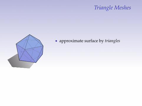
Triangle Meshes
• approximate surface by triangles
• “glued together” along edges• many possible data structures• half edge, quad edge, corner table, . . .• for simplicity: vertex-face adjacency list• (will be enough for our applications!)

Triangle Meshes
• approximate surface by triangles• “glued together” along edges
• many possible data structures• half edge, quad edge, corner table, . . .• for simplicity: vertex-face adjacency list• (will be enough for our applications!)

Triangle Meshes
• approximate surface by triangles• “glued together” along edges• many possible data structures
• half edge, quad edge, corner table, . . .• for simplicity: vertex-face adjacency list• (will be enough for our applications!)

Triangle Meshes
• approximate surface by triangles• “glued together” along edges• many possible data structures• half edge, quad edge, corner table, . . .
• for simplicity: vertex-face adjacency list• (will be enough for our applications!)

Triangle Meshes
• approximate surface by triangles• “glued together” along edges• many possible data structures• half edge, quad edge, corner table, . . .• for simplicity: vertex-face adjacency list
• (will be enough for our applications!)

Triangle Meshes
• approximate surface by triangles• “glued together” along edges• many possible data structures• half edge, quad edge, corner table, . . .• for simplicity: vertex-face adjacency list• (will be enough for our applications!)

Vertex-Face Adjacency List—Example
# xyz-coordinates of vertices
v 0 0 0
v 1 0 0
v .5 .866 0
v .5 -.866 0
# vertex-face adjacency info
f 1 2 3
f 1 4 2

Manifold

Nonmanifold

Manifold Triangle Mesh
• manifold () “locally disk-like”
• Which triangle meshes are manifold?• Two triangles per edge (no “fins”)• Every vertex looks like a “fan”• Why? Simplicity.• (Sometimes not necessary. . . )

Manifold Triangle Mesh
• manifold () “locally disk-like”• Which triangle meshes are manifold?
• Two triangles per edge (no “fins”)• Every vertex looks like a “fan”• Why? Simplicity.• (Sometimes not necessary. . . )

Manifold Triangle Mesh
• manifold () “locally disk-like”• Which triangle meshes are manifold?• Two triangles per edge (no “fins”)
• Every vertex looks like a “fan”• Why? Simplicity.• (Sometimes not necessary. . . )

Manifold Triangle Mesh
• manifold () “locally disk-like”• Which triangle meshes are manifold?• Two triangles per edge (no “fins”)• Every vertex looks like a “fan”
• Why? Simplicity.• (Sometimes not necessary. . . )

Manifold Triangle Mesh
• manifold () “locally disk-like”• Which triangle meshes are manifold?• Two triangles per edge (no “fins”)• Every vertex looks like a “fan”• Why? Simplicity.
• (Sometimes not necessary. . . )

Manifold Triangle Mesh
• manifold () “locally disk-like”• Which triangle meshes are manifold?• Two triangles per edge (no “fins”)• Every vertex looks like a “fan”• Why? Simplicity.• (Sometimes not necessary. . . )

Manifold Triangle Mesh
• manifold () “locally disk-like”• Which triangle meshes are manifold?• Two triangles per edge (no “fins”)• Every vertex looks like a “fan”• Why? Simplicity.• (Sometimes not necessary. . . )

The Cotangent Laplacian
(Assuming a manifold triangle mesh. . . )
(Du)i ⇡ 12Ai Âj2N (i)
(cot aij + cot bij)(ui � uj)
The set N (i) contains the immediate neighbors of vertex i
The quantity Ai is vertex area—for now: 1/3rd of triangle areas

The Cotangent Laplacian
(Assuming a manifold triangle mesh. . . )
(Du)i ⇡ 12Ai Âj2N (i)
(cot aij + cot bij)(ui � uj)
The set N (i) contains the immediate neighbors of vertex i
The quantity Ai is vertex area—for now: 1/3rd of triangle areas

The Cotangent Laplacian
(Assuming a manifold triangle mesh. . . )
(Du)i ⇡ 12Ai Âj2N (i)
(cot aij + cot bij)(ui � uj)
The set N (i) contains the immediate neighbors of vertex i
The quantity Ai is vertex area—for now: 1/3rd of triangle areas

Origin of the Cotan Formula?
• Many different ways to derive it
• piecewise linear finite elements (FEM)• finite volumes• discrete exterior calculus (DEC)• . . .
• Re-derived in many different contexts:• mean curvature flow [Desbrun et al., 1999]• minimal surfaces [Pinkall and Polthier, 1993]• electrical networks [Duffin, 1959]• Poisson equation [MacNeal, 1949]• (Courant? Frankel? Manhattan Project?)
• All these different viewpoints yield exact same cotan formula• For three different derivations, see [Crane et al., 2013a]

Origin of the Cotan Formula?
• Many different ways to derive it• piecewise linear finite elements (FEM)
• finite volumes• discrete exterior calculus (DEC)• . . .
• Re-derived in many different contexts:• mean curvature flow [Desbrun et al., 1999]• minimal surfaces [Pinkall and Polthier, 1993]• electrical networks [Duffin, 1959]• Poisson equation [MacNeal, 1949]• (Courant? Frankel? Manhattan Project?)
• All these different viewpoints yield exact same cotan formula• For three different derivations, see [Crane et al., 2013a]

Origin of the Cotan Formula?
• Many different ways to derive it• piecewise linear finite elements (FEM)• finite volumes
• discrete exterior calculus (DEC)• . . .
• Re-derived in many different contexts:• mean curvature flow [Desbrun et al., 1999]• minimal surfaces [Pinkall and Polthier, 1993]• electrical networks [Duffin, 1959]• Poisson equation [MacNeal, 1949]• (Courant? Frankel? Manhattan Project?)
• All these different viewpoints yield exact same cotan formula• For three different derivations, see [Crane et al., 2013a]

Origin of the Cotan Formula?
• Many different ways to derive it• piecewise linear finite elements (FEM)• finite volumes• discrete exterior calculus (DEC)
• . . .• Re-derived in many different contexts:
• mean curvature flow [Desbrun et al., 1999]• minimal surfaces [Pinkall and Polthier, 1993]• electrical networks [Duffin, 1959]• Poisson equation [MacNeal, 1949]• (Courant? Frankel? Manhattan Project?)
• All these different viewpoints yield exact same cotan formula• For three different derivations, see [Crane et al., 2013a]

Origin of the Cotan Formula?
• Many different ways to derive it• piecewise linear finite elements (FEM)• finite volumes• discrete exterior calculus (DEC)• . . .
• Re-derived in many different contexts:• mean curvature flow [Desbrun et al., 1999]• minimal surfaces [Pinkall and Polthier, 1993]• electrical networks [Duffin, 1959]• Poisson equation [MacNeal, 1949]• (Courant? Frankel? Manhattan Project?)
• All these different viewpoints yield exact same cotan formula• For three different derivations, see [Crane et al., 2013a]

Origin of the Cotan Formula?
• Many different ways to derive it• piecewise linear finite elements (FEM)• finite volumes• discrete exterior calculus (DEC)• . . .
• Re-derived in many different contexts:• mean curvature flow [Desbrun et al., 1999]
• minimal surfaces [Pinkall and Polthier, 1993]• electrical networks [Duffin, 1959]• Poisson equation [MacNeal, 1949]• (Courant? Frankel? Manhattan Project?)
• All these different viewpoints yield exact same cotan formula• For three different derivations, see [Crane et al., 2013a]

Origin of the Cotan Formula?
• Many different ways to derive it• piecewise linear finite elements (FEM)• finite volumes• discrete exterior calculus (DEC)• . . .
• Re-derived in many different contexts:• mean curvature flow [Desbrun et al., 1999]• minimal surfaces [Pinkall and Polthier, 1993]
• electrical networks [Duffin, 1959]• Poisson equation [MacNeal, 1949]• (Courant? Frankel? Manhattan Project?)
• All these different viewpoints yield exact same cotan formula• For three different derivations, see [Crane et al., 2013a]

Origin of the Cotan Formula?
• Many different ways to derive it• piecewise linear finite elements (FEM)• finite volumes• discrete exterior calculus (DEC)• . . .
• Re-derived in many different contexts:• mean curvature flow [Desbrun et al., 1999]• minimal surfaces [Pinkall and Polthier, 1993]• electrical networks [Duffin, 1959]
• Poisson equation [MacNeal, 1949]• (Courant? Frankel? Manhattan Project?)
• All these different viewpoints yield exact same cotan formula• For three different derivations, see [Crane et al., 2013a]
Origin of the Cotan Formula?
• Many different ways to derive it• piecewise linear finite elements (FEM)• finite volumes• discrete exterior calculus (DEC)• . . .
• Re-derived in many different contexts:• mean curvature flow [Desbrun et al., 1999]• minimal surfaces [Pinkall and Polthier, 1993]• electrical networks [Duffin, 1959]• Poisson equation [MacNeal, 1949]
• (Courant? Frankel? Manhattan Project?)
• All these different viewpoints yield exact same cotan formula• For three different derivations, see [Crane et al., 2013a]

Origin of the Cotan Formula?
• Many different ways to derive it• piecewise linear finite elements (FEM)• finite volumes• discrete exterior calculus (DEC)• . . .
• Re-derived in many different contexts:• mean curvature flow [Desbrun et al., 1999]• minimal surfaces [Pinkall and Polthier, 1993]• electrical networks [Duffin, 1959]• Poisson equation [MacNeal, 1949]• (Courant? Frankel? Manhattan Project?)
• All these different viewpoints yield exact same cotan formula• For three different derivations, see [Crane et al., 2013a]

Origin of the Cotan Formula?
• Many different ways to derive it• piecewise linear finite elements (FEM)• finite volumes• discrete exterior calculus (DEC)• . . .
• Re-derived in many different contexts:• mean curvature flow [Desbrun et al., 1999]• minimal surfaces [Pinkall and Polthier, 1993]• electrical networks [Duffin, 1959]• Poisson equation [MacNeal, 1949]• (Courant? Frankel? Manhattan Project?)
• All these different viewpoints yield exact same cotan formula
• For three different derivations, see [Crane et al., 2013a]

Origin of the Cotan Formula?
• Many different ways to derive it• piecewise linear finite elements (FEM)• finite volumes• discrete exterior calculus (DEC)• . . .
• Re-derived in many different contexts:• mean curvature flow [Desbrun et al., 1999]• minimal surfaces [Pinkall and Polthier, 1993]• electrical networks [Duffin, 1959]• Poisson equation [MacNeal, 1949]• (Courant? Frankel? Manhattan Project?)
• All these different viewpoints yield exact same cotan formula• For three different derivations, see [Crane et al., 2013a]

MacNeal, 1949

Cotan-Laplacian via Finite Volumes
• Integrate over each dual cell Ci
•R
CiDu =
RCi
f (“weak”)• Right-hand side approximated as Ai fi• Left-hand side becomes
RCir ·ru =
R∂Ci
n ·ru (Stokes’)• Get piecewise integral over boundary Âej2∂Ci
Rej
nj ·ru
• After some trigonometry: 12 Âj2N (i)(cot aij + cot bij)(ui� uj)
• (Can divide by Ai to approximate pointwise value)

Cotan-Laplacian via Finite Volumes
• Integrate over each dual cell Ci
•R
CiDu =
RCi
f (“weak”)
• Right-hand side approximated as Ai fi• Left-hand side becomes
RCir ·ru =
R∂Ci
n ·ru (Stokes’)• Get piecewise integral over boundary Âej2∂Ci
Rej
nj ·ru
• After some trigonometry: 12 Âj2N (i)(cot aij + cot bij)(ui� uj)
• (Can divide by Ai to approximate pointwise value)

Cotan-Laplacian via Finite Volumes
• Integrate over each dual cell Ci
•R
CiDu =
RCi
f (“weak”)• Right-hand side approximated as Ai fi
• Left-hand side becomesR
Cir ·ru =
R∂Ci
n ·ru (Stokes’)• Get piecewise integral over boundary Âej2∂Ci
Rej
nj ·ru
• After some trigonometry: 12 Âj2N (i)(cot aij + cot bij)(ui� uj)
• (Can divide by Ai to approximate pointwise value)

Cotan-Laplacian via Finite Volumes
• Integrate over each dual cell Ci
•R
CiDu =
RCi
f (“weak”)• Right-hand side approximated as Ai fi• Left-hand side becomes
RCir ·ru =
R∂Ci
n ·ru (Stokes’)
• Get piecewise integral over boundary Âej2∂Ci
Rej
nj ·ru
• After some trigonometry: 12 Âj2N (i)(cot aij + cot bij)(ui� uj)
• (Can divide by Ai to approximate pointwise value)

Cotan-Laplacian via Finite Volumes
• Integrate over each dual cell Ci
•R
CiDu =
RCi
f (“weak”)• Right-hand side approximated as Ai fi• Left-hand side becomes
RCir ·ru =
R∂Ci
n ·ru (Stokes’)• Get piecewise integral over boundary Âej2∂Ci
Rej
nj ·ru
• After some trigonometry: 12 Âj2N (i)(cot aij + cot bij)(ui� uj)
• (Can divide by Ai to approximate pointwise value)

Cotan-Laplacian via Finite Volumes
• Integrate over each dual cell Ci
•R
CiDu =
RCi
f (“weak”)• Right-hand side approximated as Ai fi• Left-hand side becomes
RCir ·ru =
R∂Ci
n ·ru (Stokes’)• Get piecewise integral over boundary Âej2∂Ci
Rej
nj ·ru
• After some trigonometry: 12 Âj2N (i)(cot aij + cot bij)(ui� uj)
• (Can divide by Ai to approximate pointwise value)

Triangle Quality—Rule of Thumb
good triangles bad triangles
(For further discussion see Shewchuk, “What Is a Good Linear Finite Element?”)

Triangle Quality—Delaunay Property
Delaunay Not Delaunay

Local Mesh Improvement
• Some simple ways to improve quality of Laplacian
• E.g., if a + b > p, “flip” the edge; after enough flips, meshwill be Delaunay [Bobenko and Springborn, 2005]
• Other ways to improve mesh (edge collapse, edge split, . . . )• Particular interest recently in interface tracking• For more, see [Dunyach et al., 2013, Wojtan et al., 2011].

Local Mesh Improvement
• Some simple ways to improve quality of Laplacian• E.g., if a + b > p, “flip” the edge; after enough flips, mesh
will be Delaunay [Bobenko and Springborn, 2005]
• Other ways to improve mesh (edge collapse, edge split, . . . )• Particular interest recently in interface tracking• For more, see [Dunyach et al., 2013, Wojtan et al., 2011].

Local Mesh Improvement
• Some simple ways to improve quality of Laplacian• E.g., if a + b > p, “flip” the edge; after enough flips, mesh
will be Delaunay [Bobenko and Springborn, 2005]• Other ways to improve mesh (edge collapse, edge split, . . . )
• Particular interest recently in interface tracking• For more, see [Dunyach et al., 2013, Wojtan et al., 2011].

Local Mesh Improvement
• Some simple ways to improve quality of Laplacian• E.g., if a + b > p, “flip” the edge; after enough flips, mesh
will be Delaunay [Bobenko and Springborn, 2005]• Other ways to improve mesh (edge collapse, edge split, . . . )• Particular interest recently in interface tracking
• For more, see [Dunyach et al., 2013, Wojtan et al., 2011].

Local Mesh Improvement
• Some simple ways to improve quality of Laplacian• E.g., if a + b > p, “flip” the edge; after enough flips, mesh
will be Delaunay [Bobenko and Springborn, 2005]• Other ways to improve mesh (edge collapse, edge split, . . . )• Particular interest recently in interface tracking• For more, see [Dunyach et al., 2013, Wojtan et al., 2011].

Meshes and Matrices
9
1011
12
1
2
34
6
78
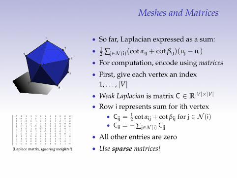
5
(Laplace matrix, ignoring weights!)
• So far, Laplacian expressed as a sum:
• 12 Âj2N (i)(cot aij + cot bij)(uj � ui)
• For computation, encode using matrices• First, give each vertex an index
1, . . . , |V|• Weak Laplacian is matrix C 2 R|V|⇥|V|
• Row i represents sum for ith vertex• Cij =
12 cot aij + cot bij for j 2 N (i)
• Cii = �Âj2N (i) Cij
• All other entries are zero• Use sparse matrices!• (MATLAB: sparse, SuiteSparse:cholmod_sparse, Eigen: SparseMatrix)

Meshes and Matrices
9
1011
12
1
2
34
6
78
5
(Laplace matrix, ignoring weights!)
• So far, Laplacian expressed as a sum:• 1
2 Âj2N (i)(cot aij + cot bij)(uj � ui)
• For computation, encode using matrices
• First, give each vertex an index1, . . . , |V|
• Weak Laplacian is matrix C 2 R|V|⇥|V|
• Row i represents sum for ith vertex• Cij =
12 cot aij + cot bij for j 2 N (i)
• Cii = �Âj2N (i) Cij
• All other entries are zero• Use sparse matrices!• (MATLAB: sparse, SuiteSparse:cholmod_sparse, Eigen: SparseMatrix)

Meshes and Matrices
9
1011
12
1
2
34
6
78
5
(Laplace matrix, ignoring weights!)
• So far, Laplacian expressed as a sum:• 1
2 Âj2N (i)(cot aij + cot bij)(uj � ui)
• For computation, encode using matrices• First, give each vertex an index
1, . . . , |V|
• Weak Laplacian is matrix C 2 R|V|⇥|V|
• Row i represents sum for ith vertex• Cij =
12 cot aij + cot bij for j 2 N (i)
• Cii = �Âj2N (i) Cij
• All other entries are zero• Use sparse matrices!• (MATLAB: sparse, SuiteSparse:cholmod_sparse, Eigen: SparseMatrix)

Meshes and Matrices
9
1011
12
1
2
34
6
78
5
(Laplace matrix, ignoring weights!)
• So far, Laplacian expressed as a sum:• 1
2 Âj2N (i)(cot aij + cot bij)(uj � ui)
• For computation, encode using matrices• First, give each vertex an index
1, . . . , |V|• Weak Laplacian is matrix C 2 R|V|⇥|V|
• Row i represents sum for ith vertex• Cij =
12 cot aij + cot bij for j 2 N (i)
• Cii = �Âj2N (i) Cij
• All other entries are zero• Use sparse matrices!• (MATLAB: sparse, SuiteSparse:cholmod_sparse, Eigen: SparseMatrix)

Meshes and Matrices
9
1011
12
1
2
34
6
78
5
(Laplace matrix, ignoring weights!)
• So far, Laplacian expressed as a sum:• 1
2 Âj2N (i)(cot aij + cot bij)(uj � ui)
• For computation, encode using matrices• First, give each vertex an index
1, . . . , |V|• Weak Laplacian is matrix C 2 R|V|⇥|V|
• Row i represents sum for ith vertex
• Cij =12 cot aij + cot bij for j 2 N (i)
• Cii = �Âj2N (i) Cij
• All other entries are zero• Use sparse matrices!• (MATLAB: sparse, SuiteSparse:cholmod_sparse, Eigen: SparseMatrix)

Meshes and Matrices
9
1011
12
1
2
34
6
78
5
(Laplace matrix, ignoring weights!)
• So far, Laplacian expressed as a sum:• 1
2 Âj2N (i)(cot aij + cot bij)(uj � ui)
• For computation, encode using matrices• First, give each vertex an index
1, . . . , |V|• Weak Laplacian is matrix C 2 R|V|⇥|V|
• Row i represents sum for ith vertex• Cij =
12 cot aij + cot bij for j 2 N (i)
• Cii = �Âj2N (i) Cij
• All other entries are zero• Use sparse matrices!• (MATLAB: sparse, SuiteSparse:cholmod_sparse, Eigen: SparseMatrix)

Meshes and Matrices
9
1011
12
1
2
34
6
78
5
(Laplace matrix, ignoring weights!)
• So far, Laplacian expressed as a sum:• 1
2 Âj2N (i)(cot aij + cot bij)(uj � ui)
• For computation, encode using matrices• First, give each vertex an index
1, . . . , |V|• Weak Laplacian is matrix C 2 R|V|⇥|V|
• Row i represents sum for ith vertex• Cij =
12 cot aij + cot bij for j 2 N (i)
• Cii = �Âj2N (i) Cij
• All other entries are zero
• Use sparse matrices!• (MATLAB: sparse, SuiteSparse:cholmod_sparse, Eigen: SparseMatrix)
Meshes and Matrices
9
1011
12
1
2
34
6
78
5
(Laplace matrix, ignoring weights!)
• So far, Laplacian expressed as a sum:• 1
2 Âj2N (i)(cot aij + cot bij)(uj � ui)
• For computation, encode using matrices• First, give each vertex an index
1, . . . , |V|• Weak Laplacian is matrix C 2 R|V|⇥|V|
• Row i represents sum for ith vertex• Cij =
12 cot aij + cot bij for j 2 N (i)
• Cii = �Âj2N (i) Cij
• All other entries are zero• Use sparse matrices!
• (MATLAB: sparse, SuiteSparse:cholmod_sparse, Eigen: SparseMatrix)

Meshes and Matrices
9
1011
12
1
2
34
6
78
5
(Laplace matrix, ignoring weights!)
• So far, Laplacian expressed as a sum:• 1
2 Âj2N (i)(cot aij + cot bij)(uj � ui)
• For computation, encode using matrices• First, give each vertex an index
1, . . . , |V|• Weak Laplacian is matrix C 2 R|V|⇥|V|
• Row i represents sum for ith vertex• Cij =
12 cot aij + cot bij for j 2 N (i)
• Cii = �Âj2N (i) Cij
• All other entries are zero• Use sparse matrices!• (MATLAB: sparse, SuiteSparse:cholmod_sparse, Eigen: SparseMatrix)

Mass Matrix
• Matrix C encodes only part of Laplacian—recall that
(Du)i = 12Ai Âj2N (i)
(cot aij + cot bij)(uj � ui)
• Still need to incorporate vertex areas Ai
• For convenience, build diagonal mass matrix M 2 R|V|⇥|V|:
M =
2
64A1
. . .A|V|
3
75
• Entries are just Mii = Ai (all other entries are zero)• Laplace operator is then L
:= M
�1C
• Applying L to a column vector u 2 R|V| “implements” thecotan formula shown above

Mass Matrix
• Matrix C encodes only part of Laplacian—recall that
(Du)i = 12Ai Âj2N (i)
(cot aij + cot bij)(uj � ui)
• Still need to incorporate vertex areas Ai
• For convenience, build diagonal mass matrix M 2 R|V|⇥|V|:
M =
2
64A1
. . .A|V|
3
75
• Entries are just Mii = Ai (all other entries are zero)
• Laplace operator is then L
:= M
�1C
• Applying L to a column vector u 2 R|V| “implements” thecotan formula shown above

Mass Matrix
• Matrix C encodes only part of Laplacian—recall that
(Du)i = 12Ai Âj2N (i)
(cot aij + cot bij)(uj � ui)
• Still need to incorporate vertex areas Ai
• For convenience, build diagonal mass matrix M 2 R|V|⇥|V|:
M =
2
64A1
. . .A|V|
3
75
• Entries are just Mii = Ai (all other entries are zero)• Laplace operator is then L
:= M
�1C
• Applying L to a column vector u 2 R|V| “implements” thecotan formula shown above

Mass Matrix
• Matrix C encodes only part of Laplacian—recall that
(Du)i = 12Ai Âj2N (i)
(cot aij + cot bij)(uj � ui)
• Still need to incorporate vertex areas Ai
• For convenience, build diagonal mass matrix M 2 R|V|⇥|V|:
M =
2
64A1
. . .A|V|
3
75
• Entries are just Mii = Ai (all other entries are zero)• Laplace operator is then L
:= M
�1C
• Applying L to a column vector u 2 R|V| “implements” thecotan formula shown above

Discrete Poisson / Laplace Equation
• Poisson equation Du = f becomes linear algebra problem:
Lu = f
• Vector f 2 R|V| is given data; u 2 R|V| is unknown.• Discrete approximation u approaches smooth solution u as
mesh is refined (for smooth data, “good” meshes. . . ).• Laplace is just Poisson with “zero” on right hand side!

Discrete Poisson / Laplace Equation
• Poisson equation Du = f becomes linear algebra problem:
Lu = f
• Vector f 2 R|V| is given data; u 2 R|V| is unknown.
• Discrete approximation u approaches smooth solution u asmesh is refined (for smooth data, “good” meshes. . . ).
• Laplace is just Poisson with “zero” on right hand side!

Discrete Poisson / Laplace Equation
• Poisson equation Du = f becomes linear algebra problem:
Lu = f
• Vector f 2 R|V| is given data; u 2 R|V| is unknown.• Discrete approximation u approaches smooth solution u as
mesh is refined (for smooth data, “good” meshes. . . ).
• Laplace is just Poisson with “zero” on right hand side!

Discrete Poisson / Laplace Equation
• Poisson equation Du = f becomes linear algebra problem:
Lu = f
• Vector f 2 R|V| is given data; u 2 R|V| is unknown.• Discrete approximation u approaches smooth solution u as
mesh is refined (for smooth data, “good” meshes. . . ).• Laplace is just Poisson with “zero” on right hand side!

Discrete Heat Equation
• Heat equation dudt = Du must also be discretized in time
• Replace time derivative with finite difference:
dudt) uk+1 � uk
h
, h > 0| {z }“time step”
• How (or really, “when”) do we approximate Du?• Explicit: (uk+1 � uk)/h = Luk (cheaper to compute)• Implicit: (uk+1 � uk)/h = Luk+1 (more stable)• Implicit update becomes linear system (I� hL)uk+1 = uk

Discrete Heat Equation
• Heat equation dudt = Du must also be discretized in time
• Replace time derivative with finite difference:
dudt) uk+1 � uk
h
, h > 0| {z }“time step”
• How (or really, “when”) do we approximate Du?
• Explicit: (uk+1 � uk)/h = Luk (cheaper to compute)• Implicit: (uk+1 � uk)/h = Luk+1 (more stable)• Implicit update becomes linear system (I� hL)uk+1 = uk

Discrete Heat Equation
• Heat equation dudt = Du must also be discretized in time
• Replace time derivative with finite difference:
dudt) uk+1 � uk
h
, h > 0| {z }“time step”
• How (or really, “when”) do we approximate Du?• Explicit: (uk+1 � uk)/h = Luk (cheaper to compute)
• Implicit: (uk+1 � uk)/h = Luk+1 (more stable)• Implicit update becomes linear system (I� hL)uk+1 = uk

Discrete Heat Equation
• Heat equation dudt = Du must also be discretized in time
• Replace time derivative with finite difference:
dudt) uk+1 � uk
h
, h > 0| {z }“time step”
• How (or really, “when”) do we approximate Du?• Explicit: (uk+1 � uk)/h = Luk (cheaper to compute)• Implicit: (uk+1 � uk)/h = Luk+1 (more stable)
• Implicit update becomes linear system (I� hL)uk+1 = uk

Discrete Heat Equation
• Heat equation dudt = Du must also be discretized in time
• Replace time derivative with finite difference:
dudt) uk+1 � uk
h
, h > 0| {z }“time step”
• How (or really, “when”) do we approximate Du?• Explicit: (uk+1 � uk)/h = Luk (cheaper to compute)• Implicit: (uk+1 � uk)/h = Luk+1 (more stable)• Implicit update becomes linear system (I� hL)uk+1 = uk

Discrete Eigenvalue Problem
• Smallest eigenvalue problem Du = lu becomes
Lu = lu
for smallest nonzero eigenvalue l.
• Can be solved using (inverse) power method:• Pick random u0• Until convergence:
• Solve Luk+1 = uk• Remove mean value from uk+1• uk+1 uk+1/|uk+1|
• By prefactoring L, overall cost is nearly identical to solvinga single Poisson equation!

Discrete Eigenvalue Problem
• Smallest eigenvalue problem Du = lu becomes
Lu = lu
for smallest nonzero eigenvalue l.• Can be solved using (inverse) power method:
• Pick random u0• Until convergence:
• Solve Luk+1 = uk• Remove mean value from uk+1• uk+1 uk+1/|uk+1|
• By prefactoring L, overall cost is nearly identical to solvinga single Poisson equation!

Properties of cotan-Laplace
• Always, always, always positive-semidefinite f
TCf � 0
(even if cotan weights are negative!)
• Why? f
TCf is identical to summing ||rf ||2!
• No boundary) constant vector in the kernel / cokernel• Why does it matter? E.g., for Poisson equation:
• solution is unique only up to constant shift• if RHS has nonzero mean, cannot be solved!
• Exhibits maximum principle on Delaunay mesh• Delaunay: triangle circumcircles are empty• Maximum principle: solution to Laplace equation has no
interior extrema (local max or min)• NOTE: non-Delaunay meshes can also exhibit max
principle! (And often do.) Delaunay sufficient but notnecessary. Currently no nice, simple necessary condition onmesh geometry.
• For more, see [Wardetzky et al., 2007]

Properties of cotan-Laplace
• Always, always, always positive-semidefinite f
TCf � 0
(even if cotan weights are negative!)• Why? f
TCf is identical to summing ||rf ||2!
• No boundary) constant vector in the kernel / cokernel
• Why does it matter? E.g., for Poisson equation:• solution is unique only up to constant shift• if RHS has nonzero mean, cannot be solved!
• Exhibits maximum principle on Delaunay mesh• Delaunay: triangle circumcircles are empty• Maximum principle: solution to Laplace equation has no
interior extrema (local max or min)• NOTE: non-Delaunay meshes can also exhibit max
principle! (And often do.) Delaunay sufficient but notnecessary. Currently no nice, simple necessary condition onmesh geometry.
• For more, see [Wardetzky et al., 2007]

Properties of cotan-Laplace
• Always, always, always positive-semidefinite f
TCf � 0
(even if cotan weights are negative!)• Why? f
TCf is identical to summing ||rf ||2!
• No boundary) constant vector in the kernel / cokernel• Why does it matter? E.g., for Poisson equation:
• solution is unique only up to constant shift• if RHS has nonzero mean, cannot be solved!
• Exhibits maximum principle on Delaunay mesh• Delaunay: triangle circumcircles are empty• Maximum principle: solution to Laplace equation has no
interior extrema (local max or min)• NOTE: non-Delaunay meshes can also exhibit max
principle! (And often do.) Delaunay sufficient but notnecessary. Currently no nice, simple necessary condition onmesh geometry.
• For more, see [Wardetzky et al., 2007]

Properties of cotan-Laplace
• Always, always, always positive-semidefinite f
TCf � 0
(even if cotan weights are negative!)• Why? f
TCf is identical to summing ||rf ||2!
• No boundary) constant vector in the kernel / cokernel• Why does it matter? E.g., for Poisson equation:
• solution is unique only up to constant shift
• if RHS has nonzero mean, cannot be solved!• Exhibits maximum principle on Delaunay mesh
• Delaunay: triangle circumcircles are empty• Maximum principle: solution to Laplace equation has no
interior extrema (local max or min)• NOTE: non-Delaunay meshes can also exhibit max
principle! (And often do.) Delaunay sufficient but notnecessary. Currently no nice, simple necessary condition onmesh geometry.
• For more, see [Wardetzky et al., 2007]

Properties of cotan-Laplace
• Always, always, always positive-semidefinite f
TCf � 0
(even if cotan weights are negative!)• Why? f
TCf is identical to summing ||rf ||2!
• No boundary) constant vector in the kernel / cokernel• Why does it matter? E.g., for Poisson equation:
• solution is unique only up to constant shift• if RHS has nonzero mean, cannot be solved!
• Exhibits maximum principle on Delaunay mesh• Delaunay: triangle circumcircles are empty• Maximum principle: solution to Laplace equation has no
interior extrema (local max or min)• NOTE: non-Delaunay meshes can also exhibit max
principle! (And often do.) Delaunay sufficient but notnecessary. Currently no nice, simple necessary condition onmesh geometry.
• For more, see [Wardetzky et al., 2007]

Properties of cotan-Laplace
• Always, always, always positive-semidefinite f
TCf � 0
(even if cotan weights are negative!)• Why? f
TCf is identical to summing ||rf ||2!
• No boundary) constant vector in the kernel / cokernel• Why does it matter? E.g., for Poisson equation:
• solution is unique only up to constant shift• if RHS has nonzero mean, cannot be solved!
• Exhibits maximum principle on Delaunay mesh
• Delaunay: triangle circumcircles are empty• Maximum principle: solution to Laplace equation has no
interior extrema (local max or min)• NOTE: non-Delaunay meshes can also exhibit max
principle! (And often do.) Delaunay sufficient but notnecessary. Currently no nice, simple necessary condition onmesh geometry.
• For more, see [Wardetzky et al., 2007]

Properties of cotan-Laplace
• Always, always, always positive-semidefinite f
TCf � 0
(even if cotan weights are negative!)• Why? f
TCf is identical to summing ||rf ||2!
• No boundary) constant vector in the kernel / cokernel• Why does it matter? E.g., for Poisson equation:
• solution is unique only up to constant shift• if RHS has nonzero mean, cannot be solved!
• Exhibits maximum principle on Delaunay mesh• Delaunay: triangle circumcircles are empty
• Maximum principle: solution to Laplace equation has nointerior extrema (local max or min)
• NOTE: non-Delaunay meshes can also exhibit maxprinciple! (And often do.) Delaunay sufficient but notnecessary. Currently no nice, simple necessary condition onmesh geometry.
• For more, see [Wardetzky et al., 2007]

Properties of cotan-Laplace
• Always, always, always positive-semidefinite f
TCf � 0
(even if cotan weights are negative!)• Why? f
TCf is identical to summing ||rf ||2!
• No boundary) constant vector in the kernel / cokernel• Why does it matter? E.g., for Poisson equation:
• solution is unique only up to constant shift• if RHS has nonzero mean, cannot be solved!
• Exhibits maximum principle on Delaunay mesh• Delaunay: triangle circumcircles are empty• Maximum principle: solution to Laplace equation has no
interior extrema (local max or min)
• NOTE: non-Delaunay meshes can also exhibit maxprinciple! (And often do.) Delaunay sufficient but notnecessary. Currently no nice, simple necessary condition onmesh geometry.
• For more, see [Wardetzky et al., 2007]

Properties of cotan-Laplace
• Always, always, always positive-semidefinite f
TCf � 0
(even if cotan weights are negative!)• Why? f
TCf is identical to summing ||rf ||2!
• No boundary) constant vector in the kernel / cokernel• Why does it matter? E.g., for Poisson equation:
• solution is unique only up to constant shift• if RHS has nonzero mean, cannot be solved!
• Exhibits maximum principle on Delaunay mesh• Delaunay: triangle circumcircles are empty• Maximum principle: solution to Laplace equation has no
interior extrema (local max or min)• NOTE: non-Delaunay meshes can also exhibit max
principle! (And often do.) Delaunay sufficient but notnecessary. Currently no nice, simple necessary condition onmesh geometry.
• For more, see [Wardetzky et al., 2007]

Properties of cotan-Laplace
• Always, always, always positive-semidefinite f
TCf � 0
(even if cotan weights are negative!)• Why? f
TCf is identical to summing ||rf ||2!
• No boundary) constant vector in the kernel / cokernel• Why does it matter? E.g., for Poisson equation:
• solution is unique only up to constant shift• if RHS has nonzero mean, cannot be solved!
• Exhibits maximum principle on Delaunay mesh• Delaunay: triangle circumcircles are empty• Maximum principle: solution to Laplace equation has no
interior extrema (local max or min)• NOTE: non-Delaunay meshes can also exhibit max
principle! (And often do.) Delaunay sufficient but notnecessary. Currently no nice, simple necessary condition onmesh geometry.
• For more, see [Wardetzky et al., 2007]

Numerical Issues—Symmetry
• “Best” case for sparse linear systems:
symmetric positive-(semi)definite (AT= A, x
TAx � 0 8x)
• Many good solvers (Cholesky, conjugate gradient, . . . )• Discrete Poisson equation looks like M
�1Cu = f
•C is symmetric, but M
�1C is not!
• Can easily be made symmetric:
Cu = Mf
• In other words: just multiply by vertex areas!• Seemingly superficial change. . .• . . . but makes computation simpler / more efficient

Numerical Issues—Symmetry
• “Best” case for sparse linear systems:
symmetric positive-(semi)definite (AT= A, x
TAx � 0 8x)
• Many good solvers (Cholesky, conjugate gradient, . . . )
• Discrete Poisson equation looks like M
�1Cu = f
•C is symmetric, but M
�1C is not!
• Can easily be made symmetric:
Cu = Mf
• In other words: just multiply by vertex areas!• Seemingly superficial change. . .• . . . but makes computation simpler / more efficient

Numerical Issues—Symmetry
• “Best” case for sparse linear systems:
symmetric positive-(semi)definite (AT= A, x
TAx � 0 8x)
• Many good solvers (Cholesky, conjugate gradient, . . . )• Discrete Poisson equation looks like M
�1Cu = f
•C is symmetric, but M
�1C is not!
• Can easily be made symmetric:
Cu = Mf
• In other words: just multiply by vertex areas!• Seemingly superficial change. . .• . . . but makes computation simpler / more efficient

Numerical Issues—Symmetry
• “Best” case for sparse linear systems:
symmetric positive-(semi)definite (AT= A, x
TAx � 0 8x)
• Many good solvers (Cholesky, conjugate gradient, . . . )• Discrete Poisson equation looks like M
�1Cu = f
•C is symmetric, but M
�1C is not!
• Can easily be made symmetric:
Cu = Mf
• In other words: just multiply by vertex areas!
• Seemingly superficial change. . .• . . . but makes computation simpler / more efficient

Numerical Issues—Symmetry
• “Best” case for sparse linear systems:
symmetric positive-(semi)definite (AT= A, x
TAx � 0 8x)
• Many good solvers (Cholesky, conjugate gradient, . . . )• Discrete Poisson equation looks like M
�1Cu = f
•C is symmetric, but M
�1C is not!
• Can easily be made symmetric:
Cu = Mf
• In other words: just multiply by vertex areas!• Seemingly superficial change. . .
• . . . but makes computation simpler / more efficient

Numerical Issues—Symmetry
• “Best” case for sparse linear systems:
symmetric positive-(semi)definite (AT= A, x
TAx � 0 8x)
• Many good solvers (Cholesky, conjugate gradient, . . . )• Discrete Poisson equation looks like M
�1Cu = f
•C is symmetric, but M
�1C is not!
• Can easily be made symmetric:
Cu = Mf
• In other words: just multiply by vertex areas!• Seemingly superficial change. . .• . . . but makes computation simpler / more efficient

Numerical Issues—Symmetry
• “Best” case for sparse linear systems:
symmetric positive-(semi)definite (AT= A, x
TAx � 0 8x)
• Many good solvers (Cholesky, conjugate gradient, . . . )• Discrete Poisson equation looks like M
�1Cu = f
•C is symmetric, but M
�1C is not!
• Can easily be made symmetric:
Cu = Mf
• In other words: just multiply by vertex areas!• Seemingly superficial change. . .• . . . but makes computation simpler / more efficient

Numerical Issues—Symmetry, continued
• Can also make heat equation symmetric
• Instead of (I� hL)uk+1 = uk, use
(M� hC)uk+1 = Muk
• What about smallest eigenvalue problem Lu = lu?• Two options:
1 Solve generalized eigenvalue problem Cu = lMu2 Solve M�1/2CM�1/2u = lu, recover u = M�1/2u
• Note: M�1/2 just means “put 1/pAi on the diagonal!”

Numerical Issues—Symmetry, continued
• Can also make heat equation symmetric• Instead of (I� hL)uk+1 = uk, use
(M� hC)uk+1 = Muk
• What about smallest eigenvalue problem Lu = lu?
• Two options:1 Solve generalized eigenvalue problem Cu = lMu2 Solve M�1/2CM�1/2u = lu, recover u = M�1/2u
• Note: M�1/2 just means “put 1/pAi on the diagonal!”

Numerical Issues—Symmetry, continued
• Can also make heat equation symmetric• Instead of (I� hL)uk+1 = uk, use
(M� hC)uk+1 = Muk
• What about smallest eigenvalue problem Lu = lu?• Two options:
1 Solve generalized eigenvalue problem Cu = lMu2 Solve M�1/2CM�1/2u = lu, recover u = M�1/2u
• Note: M�1/2 just means “put 1/pAi on the diagonal!”

Numerical Issues—Symmetry, continued
• Can also make heat equation symmetric• Instead of (I� hL)uk+1 = uk, use
(M� hC)uk+1 = Muk
• What about smallest eigenvalue problem Lu = lu?• Two options:
1 Solve generalized eigenvalue problem Cu = lMu
2 Solve M�1/2CM�1/2u = lu, recover u = M�1/2u
• Note: M�1/2 just means “put 1/pAi on the diagonal!”

Numerical Issues—Symmetry, continued
• Can also make heat equation symmetric• Instead of (I� hL)uk+1 = uk, use
(M� hC)uk+1 = Muk
• What about smallest eigenvalue problem Lu = lu?• Two options:
1 Solve generalized eigenvalue problem Cu = lMu2 Solve M�1/2CM�1/2u = lu, recover u = M�1/2u
• Note: M�1/2 just means “put 1/pAi on the diagonal!”

Numerical Issues—Symmetry, continued
• Can also make heat equation symmetric• Instead of (I� hL)uk+1 = uk, use
(M� hC)uk+1 = Muk
• What about smallest eigenvalue problem Lu = lu?• Two options:
1 Solve generalized eigenvalue problem Cu = lMu2 Solve M�1/2CM�1/2u = lu, recover u = M�1/2u
• Note: M�1/2 just means “put 1/pAi on the diagonal!”

Numerical Issues—Direct vs. Iterative Solvers
• Direct (e.g., LLT, LU, QR, . . . )
• pros: great for multiple right-hand sides; (can be) lesssensitive to numerical instability; solve many types ofproblems, under/overdetermined systems.
• cons: prohibitively expensive for large problems; factorsare quite dense for 3D (volumetric) problems
• Iterative (e.g., conjugate gradient, multigrid, . . . )• pros: can handle very large problems; can be implemented
via callback (instead of matrix); asymptotic running timesapproaching linear time (in theory. . . )
• cons: poor performance without good preconditioners; lessbenefit for multiple right-hand sides; best-in-class methodsmay handle only symmetric positive-(semi)definite systems
• No perfect solution! Each problem is different.

Numerical Issues—Direct vs. Iterative Solvers
• Direct (e.g., LLT, LU, QR, . . . )• pros: great for multiple right-hand sides; (can be) less
sensitive to numerical instability; solve many types ofproblems, under/overdetermined systems.
• cons: prohibitively expensive for large problems; factorsare quite dense for 3D (volumetric) problems
• Iterative (e.g., conjugate gradient, multigrid, . . . )
• pros: can handle very large problems; can be implementedvia callback (instead of matrix); asymptotic running timesapproaching linear time (in theory. . . )
• cons: poor performance without good preconditioners; lessbenefit for multiple right-hand sides; best-in-class methodsmay handle only symmetric positive-(semi)definite systems
• No perfect solution! Each problem is different.

Numerical Issues—Direct vs. Iterative Solvers
• Direct (e.g., LLT, LU, QR, . . . )• pros: great for multiple right-hand sides; (can be) less
sensitive to numerical instability; solve many types ofproblems, under/overdetermined systems.
• cons: prohibitively expensive for large problems; factorsare quite dense for 3D (volumetric) problems
• Iterative (e.g., conjugate gradient, multigrid, . . . )• pros: can handle very large problems; can be implemented
via callback (instead of matrix); asymptotic running timesapproaching linear time (in theory. . . )
• cons: poor performance without good preconditioners; lessbenefit for multiple right-hand sides; best-in-class methodsmay handle only symmetric positive-(semi)definite systems
• No perfect solution! Each problem is different.

Numerical Issues—Direct vs. Iterative Solvers
• Direct (e.g., LLT, LU, QR, . . . )• pros: great for multiple right-hand sides; (can be) less
sensitive to numerical instability; solve many types ofproblems, under/overdetermined systems.
• cons: prohibitively expensive for large problems; factorsare quite dense for 3D (volumetric) problems
• Iterative (e.g., conjugate gradient, multigrid, . . . )• pros: can handle very large problems; can be implemented
via callback (instead of matrix); asymptotic running timesapproaching linear time (in theory. . . )
• cons: poor performance without good preconditioners; lessbenefit for multiple right-hand sides; best-in-class methodsmay handle only symmetric positive-(semi)definite systems
• No perfect solution! Each problem is different.

Solving Equations in Linear Time
• Is solving Poisson, Laplace, etc., truly linear time in 2D?
• Jury is still out, but keep inching forward:• [Vaidya, 1991]—use spanning tree as preconditioner• [Alon et al., 1995]—use low-stretch spanning trees• [Spielman and Teng, 2004]—first “nearly linear time” solver• [Krishnan et al., 2013]—practical solver for graphics• Lots of recent activity in both preconditioners and direct
solvers (e.g., [Koutis et al., 2011],[Gillman and Martinsson, 2013])
• Best theoretical results may lack practical implementations!• Older codes benefit from extensive low-level optimization• Long term: probably indistinguishable from O(n)

Solving Equations in Linear Time
• Is solving Poisson, Laplace, etc., truly linear time in 2D?• Jury is still out, but keep inching forward:
• [Vaidya, 1991]—use spanning tree as preconditioner• [Alon et al., 1995]—use low-stretch spanning trees• [Spielman and Teng, 2004]—first “nearly linear time” solver• [Krishnan et al., 2013]—practical solver for graphics• Lots of recent activity in both preconditioners and direct
solvers (e.g., [Koutis et al., 2011],[Gillman and Martinsson, 2013])
• Best theoretical results may lack practical implementations!
• Older codes benefit from extensive low-level optimization• Long term: probably indistinguishable from O(n)

Solving Equations in Linear Time
• Is solving Poisson, Laplace, etc., truly linear time in 2D?• Jury is still out, but keep inching forward:
• [Vaidya, 1991]—use spanning tree as preconditioner• [Alon et al., 1995]—use low-stretch spanning trees• [Spielman and Teng, 2004]—first “nearly linear time” solver• [Krishnan et al., 2013]—practical solver for graphics• Lots of recent activity in both preconditioners and direct
solvers (e.g., [Koutis et al., 2011],[Gillman and Martinsson, 2013])
• Best theoretical results may lack practical implementations!• Older codes benefit from extensive low-level optimization
• Long term: probably indistinguishable from O(n)

Solving Equations in Linear Time
• Is solving Poisson, Laplace, etc., truly linear time in 2D?• Jury is still out, but keep inching forward:
• [Vaidya, 1991]—use spanning tree as preconditioner• [Alon et al., 1995]—use low-stretch spanning trees• [Spielman and Teng, 2004]—first “nearly linear time” solver• [Krishnan et al., 2013]—practical solver for graphics• Lots of recent activity in both preconditioners and direct
solvers (e.g., [Koutis et al., 2011],[Gillman and Martinsson, 2013])
• Best theoretical results may lack practical implementations!• Older codes benefit from extensive low-level optimization• Long term: probably indistinguishable from O(n)

Boundary Conditions
• PDE (Laplace, Poisson, heat equation, etc.) determinesbehavior “inside” domain W
• Also need to say how solution behaves on boundary ∂W• Often trickiest part (both mathematically & numerically)• Very easy to get wrong!

Boundary Conditions
• PDE (Laplace, Poisson, heat equation, etc.) determinesbehavior “inside” domain W
• Also need to say how solution behaves on boundary ∂W
• Often trickiest part (both mathematically & numerically)• Very easy to get wrong!

Boundary Conditions
• PDE (Laplace, Poisson, heat equation, etc.) determinesbehavior “inside” domain W
• Also need to say how solution behaves on boundary ∂W• Often trickiest part (both mathematically & numerically)
• Very easy to get wrong!

Boundary Conditions
• PDE (Laplace, Poisson, heat equation, etc.) determinesbehavior “inside” domain W
• Also need to say how solution behaves on boundary ∂W• Often trickiest part (both mathematically & numerically)• Very easy to get wrong!

Dirichlet Boundary Conditions
• “Dirichlet” () prescribe values
• E.g., f(0) = a, f(1) = b• (Many possible functions “in between!”)

Dirichlet Boundary Conditions
• “Dirichlet” () prescribe values• E.g., f(0) = a, f(1) = b
• (Many possible functions “in between!”)

Dirichlet Boundary Conditions
• “Dirichlet” () prescribe values• E.g., f(0) = a, f(1) = b• (Many possible functions “in between!”)

Neumann Boundary Conditions
• “Neumann” () prescribe derivatives
• E.g., f0(0) = u, f0(1) = v• (Again, many possible solutions.)

Neumann Boundary Conditions
• “Neumann” () prescribe derivatives• E.g., f0(0) = u, f0(1) = v
• (Again, many possible solutions.)

Neumann Boundary Conditions
• “Neumann” () prescribe derivatives• E.g., f0(0) = u, f0(1) = v• (Again, many possible solutions.)

Both Neumann & Dirichlet
• Or: prescribe some values, some derivatives
• E.g., f0(0) = u, f(1) = b• (What about f0(1) = v, f(1) = b?)

Both Neumann & Dirichlet
• Or: prescribe some values, some derivatives• E.g., f0(0) = u, f(1) = b
• (What about f0(1) = v, f(1) = b?)

Both Neumann & Dirichlet
• Or: prescribe some values, some derivatives• E.g., f0(0) = u, f(1) = b• (What about f0(1) = v, f(1) = b?)

Laplace w/ Dirichlet Boundary Conditions (1D)
• 1D Laplace: ∂2f/∂x2 = 0
• Solutions: f(x) = cx + d (linear functions)• Can we always satisfy Dirichlet boundary conditions?
• Yes: a line can interpolate any two points

Laplace w/ Dirichlet Boundary Conditions (1D)
• 1D Laplace: ∂2f/∂x2 = 0• Solutions: f(x) = cx + d (linear functions)
• Can we always satisfy Dirichlet boundary conditions?
• Yes: a line can interpolate any two points

Laplace w/ Dirichlet Boundary Conditions (1D)
• 1D Laplace: ∂2f/∂x2 = 0• Solutions: f(x) = cx + d (linear functions)• Can we always satisfy Dirichlet boundary conditions?
• Yes: a line can interpolate any two points

Laplace w/ Dirichlet Boundary Conditions (1D)
• 1D Laplace: ∂2f/∂x2 = 0• Solutions: f(x) = cx + d (linear functions)• Can we always satisfy Dirichlet boundary conditions?
• Yes: a line can interpolate any two points

Laplace w/ Neumann Boundary Conditions (1D)
• What about Neumann boundary conditions?
• Solution must still be a line: f(x) = cx + d• Can we prescribe the derivative at both ends?
• No! A line can have only one slope!• In general: solutions to PDE may not exist for given BCs

Laplace w/ Neumann Boundary Conditions (1D)
• What about Neumann boundary conditions?• Solution must still be a line: f(x) = cx + d
• Can we prescribe the derivative at both ends?
• No! A line can have only one slope!• In general: solutions to PDE may not exist for given BCs

Laplace w/ Neumann Boundary Conditions (1D)
• What about Neumann boundary conditions?• Solution must still be a line: f(x) = cx + d• Can we prescribe the derivative at both ends?
• No! A line can have only one slope!• In general: solutions to PDE may not exist for given BCs

Laplace w/ Neumann Boundary Conditions (1D)
• What about Neumann boundary conditions?• Solution must still be a line: f(x) = cx + d• Can we prescribe the derivative at both ends?
• No! A line can have only one slope!
• In general: solutions to PDE may not exist for given BCs

Laplace w/ Neumann Boundary Conditions (1D)
• What about Neumann boundary conditions?• Solution must still be a line: f(x) = cx + d• Can we prescribe the derivative at both ends?
• No! A line can have only one slope!• In general: solutions to PDE may not exist for given BCs

Laplace w/ Dirichlet Boundary Conditions (2D)
• 2D Laplace: Df = 0
• Can we always satisfy Dirichlet boundary conditions?• Yes: Laplace is steady-state solution to heat flow d
dt f = Df
• Dirichlet data is just “heat” along boundary

Laplace w/ Dirichlet Boundary Conditions (2D)
• 2D Laplace: Df = 0• Can we always satisfy Dirichlet boundary conditions?
• Yes: Laplace is steady-state solution to heat flow ddt f = Df
• Dirichlet data is just “heat” along boundary

Laplace w/ Dirichlet Boundary Conditions (2D)
• 2D Laplace: Df = 0• Can we always satisfy Dirichlet boundary conditions?• Yes: Laplace is steady-state solution to heat flow d
dt f = Df
• Dirichlet data is just “heat” along boundary

Laplace w/ Neumann Boundary Conditions (2D)
• What about Neumann boundaryconditions?
• Still want to solve Df = 0• Want to prescribe normal derivative
n ·rf
• Wasn’t always possible in 1D. . .• In 2D, we have divergence theorem:
Z
W0 !=
Z
WDf =
Z
Wr ·rf =
Z
∂Wn ·rf
• Conclusion: can only solve Df = 0 ifNeumann BCs have zero mean!

Laplace w/ Neumann Boundary Conditions (2D)
• What about Neumann boundaryconditions?
• Still want to solve Df = 0• Want to prescribe normal derivative
n ·rf
• Wasn’t always possible in 1D. . .
• In 2D, we have divergence theorem:Z
W0 !=
Z
WDf =
Z
Wr ·rf =
Z
∂Wn ·rf
• Conclusion: can only solve Df = 0 ifNeumann BCs have zero mean!

Laplace w/ Neumann Boundary Conditions (2D)
• What about Neumann boundaryconditions?
• Still want to solve Df = 0• Want to prescribe normal derivative
n ·rf
• Wasn’t always possible in 1D. . .• In 2D, we have divergence theorem:
Z
W0 !=
Z
WDf =
Z
Wr ·rf =
Z
∂Wn ·rf
• Conclusion: can only solve Df = 0 ifNeumann BCs have zero mean!

Laplace w/ Neumann Boundary Conditions (2D)
• What about Neumann boundaryconditions?
• Still want to solve Df = 0• Want to prescribe normal derivative
n ·rf
• Wasn’t always possible in 1D. . .• In 2D, we have divergence theorem:
Z
W0 !=
Z
WDf =
Z
Wr ·rf =
Z
∂Wn ·rf
• Conclusion: can only solve Df = 0 ifNeumann BCs have zero mean!

Discrete Boundary Conditions - Dirichlet
• Suppose we want to solve Du = f s.t. u|∂W = g (Poissonequation w/ Dirichlet boundary conditions)
• Discretized Poisson equation as Cu = Mf
• Let I, B denote interior, boundary vertices, respectively. Get"
CII CIB
CBI CBB
# "uI
uB
#=
"MII 00 MBB
# "fI
fB
#
• Since uB is known (boundary values), solve justCIIuI = MIIfI � CIBuB for uI (right-hand side is known).
• Can skip matrix multiply and compute entries of RHSdirectly: Aifi �Âj2N∂(i)(cot aij + cot bij)uj
• Here N∂(i) denotes neighbors of i on the boundary

Discrete Boundary Conditions - Neumann
• Integrate both sides of Du = f over cell Ci (“finite volume”)Z
Ci
f !=
Z
Ci
Du =Z
Ci
r ·ru =Z
∂Ci
n ·ru
• Gives usual cotangent formula for interior vertices; forboundary vertex i, yields
Aii!= 1
2 (ga + gb) +12 Â
j2Nint
(cot aij + cot bij)(uj � ui)
• Here ga, gb are prescribed normal derivatives; just subtractfrom RHS and solve Cu = Mf as usual

Discrete Boundary Conditions - Neumann
• Other possible boundary conditions (e.g., Robin)
• Dirichlet, Neumann most common—implementation ofother BCs will be similar
• When in doubt, return to smooth equations and integrate!• . . . and make sure your equation has a solution!• Solver will NOT always tell you if there’s a problem!• Easy test? Compute the residual r := Ax� b. If the relative
residual ||r||•/||b||• is far from zero (e.g., greater than10�14 in double precision), you did not actually solve yourproblem!

Discrete Boundary Conditions - Neumann
• Other possible boundary conditions (e.g., Robin)• Dirichlet, Neumann most common—implementation of
other BCs will be similar
• When in doubt, return to smooth equations and integrate!• . . . and make sure your equation has a solution!• Solver will NOT always tell you if there’s a problem!• Easy test? Compute the residual r := Ax� b. If the relative
residual ||r||•/||b||• is far from zero (e.g., greater than10�14 in double precision), you did not actually solve yourproblem!

Discrete Boundary Conditions - Neumann
• Other possible boundary conditions (e.g., Robin)• Dirichlet, Neumann most common—implementation of
other BCs will be similar• When in doubt, return to smooth equations and integrate!
• . . . and make sure your equation has a solution!• Solver will NOT always tell you if there’s a problem!• Easy test? Compute the residual r := Ax� b. If the relative
residual ||r||•/||b||• is far from zero (e.g., greater than10�14 in double precision), you did not actually solve yourproblem!

Discrete Boundary Conditions - Neumann
• Other possible boundary conditions (e.g., Robin)• Dirichlet, Neumann most common—implementation of
other BCs will be similar• When in doubt, return to smooth equations and integrate!• . . . and make sure your equation has a solution!
• Solver will NOT always tell you if there’s a problem!• Easy test? Compute the residual r := Ax� b. If the relative
residual ||r||•/||b||• is far from zero (e.g., greater than10�14 in double precision), you did not actually solve yourproblem!

Discrete Boundary Conditions - Neumann
• Other possible boundary conditions (e.g., Robin)• Dirichlet, Neumann most common—implementation of
other BCs will be similar• When in doubt, return to smooth equations and integrate!• . . . and make sure your equation has a solution!• Solver will NOT always tell you if there’s a problem!
• Easy test? Compute the residual r := Ax� b. If the relativeresidual ||r||•/||b||• is far from zero (e.g., greater than10�14 in double precision), you did not actually solve yourproblem!

Discrete Boundary Conditions - Neumann
• Other possible boundary conditions (e.g., Robin)• Dirichlet, Neumann most common—implementation of
other BCs will be similar• When in doubt, return to smooth equations and integrate!• . . . and make sure your equation has a solution!• Solver will NOT always tell you if there’s a problem!• Easy test? Compute the residual r := Ax� b. If the relative
residual ||r||•/||b||• is far from zero (e.g., greater than10�14 in double precision), you did not actually solve yourproblem!

Discrete Boundary Conditions - Neumann
• Other possible boundary conditions (e.g., Robin)• Dirichlet, Neumann most common—implementation of
other BCs will be similar• When in doubt, return to smooth equations and integrate!• . . . and make sure your equation has a solution!• Solver will NOT always tell you if there’s a problem!• Easy test? Compute the residual r := Ax� b. If the relative
residual ||r||•/||b||• is far from zero (e.g., greater than10�14 in double precision), you did not actually solve yourproblem!

Alternative Discretizations
• Have spent a lot of time on triangle meshes. . .
• . . . plenty of other ways to describe a surface!• E.g., points are increasingly popular (due to 3D scanning)• Also: more accurate discretization on triangle meshes

Alternative Discretizations
• Have spent a lot of time on triangle meshes. . .• . . . plenty of other ways to describe a surface!
• E.g., points are increasingly popular (due to 3D scanning)• Also: more accurate discretization on triangle meshes

Alternative Discretizations
• Have spent a lot of time on triangle meshes. . .• . . . plenty of other ways to describe a surface!• E.g., points are increasingly popular (due to 3D scanning)
• Also: more accurate discretization on triangle meshes

Alternative Discretizations
• Have spent a lot of time on triangle meshes. . .• . . . plenty of other ways to describe a surface!• E.g., points are increasingly popular (due to 3D scanning)• Also: more accurate discretization on triangle meshes

Quad, Polygon Meshes
• Quads popular alternative to triangles.Why?
• capture principal curvatures of a surface• nice bases can be built via tensor
products• see [Bommes et al., 2013] for further
discussion
• More generally: meshes with quads andtriangles and . . .
• Nice discretization:[Alexa and Wardetzky, 2011]
• Can then solve all the same problems(Laplace, Poisson, heat, . . . )

Quad, Polygon Meshes
• Quads popular alternative to triangles.Why?
• capture principal curvatures of a surface
• nice bases can be built via tensorproducts
• see [Bommes et al., 2013] for furtherdiscussion
• More generally: meshes with quads andtriangles and . . .
• Nice discretization:[Alexa and Wardetzky, 2011]
• Can then solve all the same problems(Laplace, Poisson, heat, . . . )

Quad, Polygon Meshes
• Quads popular alternative to triangles.Why?
• capture principal curvatures of a surface• nice bases can be built via tensor
products
• see [Bommes et al., 2013] for furtherdiscussion
• More generally: meshes with quads andtriangles and . . .
• Nice discretization:[Alexa and Wardetzky, 2011]
• Can then solve all the same problems(Laplace, Poisson, heat, . . . )

Quad, Polygon Meshes
• Quads popular alternative to triangles.Why?
• capture principal curvatures of a surface• nice bases can be built via tensor
products• see [Bommes et al., 2013] for further
discussion
• More generally: meshes with quads andtriangles and . . .
• Nice discretization:[Alexa and Wardetzky, 2011]
• Can then solve all the same problems(Laplace, Poisson, heat, . . . )

Quad, Polygon Meshes
• Quads popular alternative to triangles.Why?
• capture principal curvatures of a surface• nice bases can be built via tensor
products• see [Bommes et al., 2013] for further
discussion
• More generally: meshes with quads andtriangles and . . .
• Nice discretization:[Alexa and Wardetzky, 2011]
• Can then solve all the same problems(Laplace, Poisson, heat, . . . )

Point Clouds
• Real data often point cloud with noconnectivity (plus noise, holes. . . )
• Can still build Laplace operator!• Rough idea: use heat flow to discretize D• d
dt u = Du =) Du ⇡ (u(T)� u(0))/T• How do we get u(T)? Convolve u with
(Euclidean) heat kernel 14pT er2/4T
• Converges with more samples, T goesto zero (under certain conditions!)
• Details: [Belkin et al., 2009, Liu et al., 2012]
• From there, solve all the sameproblems! (Again.)

Point Clouds
• Real data often point cloud with noconnectivity (plus noise, holes. . . )
• Can still build Laplace operator!
• Rough idea: use heat flow to discretize D• d
dt u = Du =) Du ⇡ (u(T)� u(0))/T• How do we get u(T)? Convolve u with
(Euclidean) heat kernel 14pT er2/4T
• Converges with more samples, T goesto zero (under certain conditions!)
• Details: [Belkin et al., 2009, Liu et al., 2012]
• From there, solve all the sameproblems! (Again.)

Point Clouds
• Real data often point cloud with noconnectivity (plus noise, holes. . . )
• Can still build Laplace operator!• Rough idea: use heat flow to discretize D
• ddt u = Du =) Du ⇡ (u(T)� u(0))/T
• How do we get u(T)? Convolve u with(Euclidean) heat kernel 1
4pT er2/4T
• Converges with more samples, T goesto zero (under certain conditions!)
• Details: [Belkin et al., 2009, Liu et al., 2012]
• From there, solve all the sameproblems! (Again.)

Point Clouds
• Real data often point cloud with noconnectivity (plus noise, holes. . . )
• Can still build Laplace operator!• Rough idea: use heat flow to discretize D• d
dt u = Du =) Du ⇡ (u(T)� u(0))/T
• How do we get u(T)? Convolve u with(Euclidean) heat kernel 1
4pT er2/4T
• Converges with more samples, T goesto zero (under certain conditions!)
• Details: [Belkin et al., 2009, Liu et al., 2012]
• From there, solve all the sameproblems! (Again.)

Point Clouds
• Real data often point cloud with noconnectivity (plus noise, holes. . . )
• Can still build Laplace operator!• Rough idea: use heat flow to discretize D• d
dt u = Du =) Du ⇡ (u(T)� u(0))/T• How do we get u(T)? Convolve u with
(Euclidean) heat kernel 14pT er2/4T
• Converges with more samples, T goesto zero (under certain conditions!)
• Details: [Belkin et al., 2009, Liu et al., 2012]
• From there, solve all the sameproblems! (Again.)

Point Clouds
• Real data often point cloud with noconnectivity (plus noise, holes. . . )
• Can still build Laplace operator!• Rough idea: use heat flow to discretize D• d
dt u = Du =) Du ⇡ (u(T)� u(0))/T• How do we get u(T)? Convolve u with
(Euclidean) heat kernel 14pT er2/4T
• Converges with more samples, T goesto zero (under certain conditions!)
• Details: [Belkin et al., 2009, Liu et al., 2012]
• From there, solve all the sameproblems! (Again.)

Dual Mesh
barycentric circumcentric (superimposed)
• Earlier saw Laplacian discretized via dual mesh
• Different duals lead to operators with different accuracy• Space of orthogonal duals explored by [Mullen et al., 2011]• Leads to many applications in geometry processing
[de Goes et al., 2012, de Goes et al., 2013, de Goes et al., 2014]

Dual Mesh
barycentric circumcentric (superimposed)
• Earlier saw Laplacian discretized via dual mesh• Different duals lead to operators with different accuracy
• Space of orthogonal duals explored by [Mullen et al., 2011]• Leads to many applications in geometry processing
[de Goes et al., 2012, de Goes et al., 2013, de Goes et al., 2014]

Dual Mesh
barycentric circumcentric (superimposed)
• Earlier saw Laplacian discretized via dual mesh• Different duals lead to operators with different accuracy• Space of orthogonal duals explored by [Mullen et al., 2011]
• Leads to many applications in geometry processing[de Goes et al., 2012, de Goes et al., 2013, de Goes et al., 2014]

Dual Mesh
barycentric circumcentric (superimposed)
• Earlier saw Laplacian discretized via dual mesh• Different duals lead to operators with different accuracy• Space of orthogonal duals explored by [Mullen et al., 2011]• Leads to many applications in geometry processing
[de Goes et al., 2012, de Goes et al., 2013, de Goes et al., 2014]

Volumes / Tetrahedral Meshes
• Same problems (Poisson, Laplace, etc.)can also be solved on volumes
• Popular choice: tetrahedral meshes(graded, conform to boundary, . . . )
• Many ways to get Laplace matrix• One nice way: discrete exterior calculus
(DEC) [Hirani, 2003, Desbrun et al., 2005]
• Just incidence matrices (e.g., which tetscontain which triangles?) & primal /dual volumes (area, length, etc.).
• Added bonus: play with definition ofdual to improve accuracy[Mullen et al., 2011].

Volumes / Tetrahedral Meshes
• Same problems (Poisson, Laplace, etc.)can also be solved on volumes
• Popular choice: tetrahedral meshes(graded, conform to boundary, . . . )
• Many ways to get Laplace matrix
• One nice way: discrete exterior calculus(DEC) [Hirani, 2003, Desbrun et al., 2005]
• Just incidence matrices (e.g., which tetscontain which triangles?) & primal /dual volumes (area, length, etc.).
• Added bonus: play with definition ofdual to improve accuracy[Mullen et al., 2011].
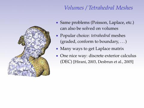
Volumes / Tetrahedral Meshes
• Same problems (Poisson, Laplace, etc.)can also be solved on volumes
• Popular choice: tetrahedral meshes(graded, conform to boundary, . . . )
• Many ways to get Laplace matrix• One nice way: discrete exterior calculus
(DEC) [Hirani, 2003, Desbrun et al., 2005]
• Just incidence matrices (e.g., which tetscontain which triangles?) & primal /dual volumes (area, length, etc.).
• Added bonus: play with definition ofdual to improve accuracy[Mullen et al., 2011].

Volumes / Tetrahedral Meshes
• Same problems (Poisson, Laplace, etc.)can also be solved on volumes
• Popular choice: tetrahedral meshes(graded, conform to boundary, . . . )
• Many ways to get Laplace matrix• One nice way: discrete exterior calculus
(DEC) [Hirani, 2003, Desbrun et al., 2005]
• Just incidence matrices (e.g., which tetscontain which triangles?) & primal /dual volumes (area, length, etc.).
• Added bonus: play with definition ofdual to improve accuracy[Mullen et al., 2011].

...and More!
• Covered some standard discretizations
• Many possibilities (level sets, hexmeshes. . . )
• Often enough to have gradient G andinner product W.
• (weak!) Laplacian is then C = G
TWG
(think Dirichlet energy)• Key message:
build Laplace; do lots of cool stuff.
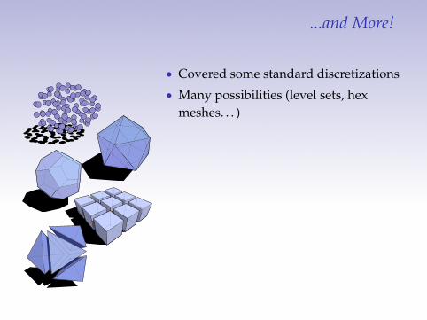
...and More!
• Covered some standard discretizations• Many possibilities (level sets, hex
meshes. . . )
• Often enough to have gradient G andinner product W.
• (weak!) Laplacian is then C = G
TWG
(think Dirichlet energy)• Key message:
build Laplace; do lots of cool stuff.

...and More!
• Covered some standard discretizations• Many possibilities (level sets, hex
meshes. . . )• Often enough to have gradient G and
inner product W.
• (weak!) Laplacian is then C = G
TWG
(think Dirichlet energy)• Key message:
build Laplace; do lots of cool stuff.

...and More!
• Covered some standard discretizations• Many possibilities (level sets, hex
meshes. . . )• Often enough to have gradient G and
inner product W.• (weak!) Laplacian is then C = G
TWG
(think Dirichlet energy)
• Key message:build Laplace; do lots of cool stuff.

...and More!
• Covered some standard discretizations• Many possibilities (level sets, hex
meshes. . . )• Often enough to have gradient G and
inner product W.• (weak!) Laplacian is then C = G
TWG
(think Dirichlet energy)• Key message:
build Laplace; do lots of cool stuff.
APPLICATIONS

Remarkably Common Pipeline
{simple pre-processing}
�!D(�1)
�! {simple post-processing}

Common Refrain
“Our method boils down to‘backslash’ in Matlab!”

Reminder: Model Equations
Df = 0 Laplace equationLinear solve
Df = g Poisson equationLinear solve
ft = Df Heat equationODE time-step
Dfi = lifi Vibration modesEigenproblem

Reminder: Model Equations
Df = 0 Laplace equationLinear solve
Df = g Poisson equationLinear solve
ft = Df Heat equationODE time-step
Dfi = lifi Vibration modesEigenproblem
Look here!

Reminder: Model Equations
Df = 0 Laplace equationLinear solve
Df = g Poisson equationLinear solve
ft = Df Heat equationODE time-step
Dfi = lifi Vibration modesEigenproblem

Reminder: Variational Interpretation
minf (x)R
S krf (x)k2 dAl <calculus>
Df (x) = 0
The (inverse) Laplacian wants tomake functions smooth.
“Elliptic regularity”
Df = 0

Reminder: Variational Interpretation
minf (x)R
S krf (x)k2 dAl <calculus>
Df (x) = 0
The (inverse) Laplacian wants tomake functions smooth.
“Elliptic regularity”
Df = 0

Application: Mesh Parameterization
Want smooth f : M! R2.
Df = 0

Variational Approach
minf :M!R2Rkrfk2
Does this work?
f (x) ⌘ const.
Df = 0

Variational Approach
minf :M!R2Rkrfk2
Does this work?
f (x) ⌘ const.
Df = 0

Harmonic Parameterization
min f :M!R2
f |∂M fixed
Rkrfk2
[Eck et al., 1995]
Df = 0 in M\∂M, with f |∂M fixed
Df = 0

Harmonic Parameterization
min f :M!R2
f |∂M fixed
Rkrfk2
[Eck et al., 1995]
Df = 0 in M\∂M, with f |∂M fixed
Df = 0

Reminder: Model Equations
Df = 0 Laplace equationLinear solve
Df = g Poisson equationLinear solve
ft = Df Heat equationODE time-step
Dfi = lifi Vibration modesEigenproblem

Recall: Green’s Function
Dgp = dp for p 2 M
Df = g

Application: Biharmonic Distances
db(p, q) ⌘ kgp� gqk2
[Lipman et al., 2010], formula in [Solomon et al., 2014]
Df = g

Hodge Decomposition
~v(x) = R90�rg +rf +~h(x)
• Divergence-free part: R90�rg• Curl-free part: rf• Harmonic part:~h(x) (=~0 if surface has no holes)
Df = g

Computing the Curl-Free Part
minf (x)R
S krf (x)�~v(x)k2 dAl <calculus>
Df (x) = r ·~v(x)Get divergence-free part as~v(x)�rf (x) (when~h ⌘~0)
Df = g

Application: Vector Field Design
Df = �K �!~v(x) = rf (x)
[Crane et al., 2010, de Goes and Crane, 2010]
Df = g

Application: Earth Mover’s Distance
min~J(x)
Z
Mk~J(x)k
such that~J = R90�rg +rf +~h(x)Df = r1 � r0
[Solomon et al., 2014]
Df = g

Reminder: Model Equations
Df = 0 Laplace equationLinear solve
Df = g Poisson equationLinear solve
ft = Df Heat equationODE time-step
Dfi = lifi Vibration modesEigenproblem

Generalizing Gaussian Blurs
Gradient descent onRkrf (x)k2 dx:
∂f (x,t)∂t = Dxf (x, t)
with f (·, 0) ⌘ f0(·).
Image by M. Bottazzi
ft = Df

Application: Implicit Fairing
Idea: Take f0(x) to be the coordinate function.
Detail: D changes over time.[Desbrun et al., 1999]
ft = Df

Application: Implicit Fairing
Idea: Take f0(x) to be the coordinate function.Detail: D changes over time.
[Desbrun et al., 1999]
ft = Df

Alternative: Screened Poisson Smoothing
Simplest incarnation of [Chuang and Kazhdan, 2011]:
minf (x) a2kf � f0k2 + krfk2
l
(a2I� D)f = a2f0
Df = g

Interesting Connection
(Semi-)Implicit Euler:(I� hL)uk+1 = uk
Screened Poisson:(a2I� D)f = a2f0
One time step of implicit Euleris screened Poisson.
Accidentally replaced one PDE with another!
ft = Df ! Df = g

Interesting Connection
(Semi-)Implicit Euler:(I� hL)uk+1 = uk
Screened Poisson:(a2I� D)f = a2f0
One time step of implicit Euleris screened Poisson.
Accidentally replaced one PDE with another!
ft = Df ! Df = g

Interesting Connection
(Semi-)Implicit Euler:(I� hL)uk+1 = uk
Screened Poisson:(a2I� D)f = a2f0
One time step of implicit Euleris screened Poisson.
Accidentally replaced one PDE with another!
ft = Df ! Df = g

Application: The “Heat Method”
Eikonal equation for geodesics:krfk2 = 1
=) Need direction of rf.
Idea:Find u such that ru is parallel to
geodesic.
ft = Df and Df = g

Application: The “Heat Method”
Eikonal equation for geodesics:krfk2 = 1
=) Need direction of rf.
Idea:Find u such that ru is parallel to
geodesic.
ft = Df and Df = g

Application: The “Heat Method”
1 Integrate u0 = ru (heat equation) to time t⌧ 1.
2 Define vector field X ⌘ � rukruk2
.
3 Solve least-squares problem rf ⇡ X () Df = r · X.
Blazingly fast![Crane et al., 2013b]
ft = Df and Df = g

Reminder: Model Equations
Df = 0 Laplace equationLinear solve
Df = g Poisson equationLinear solve
ft = Df Heat equationODE time-step
Dfi = lifi Vibration modesEigenproblem

Laplace-Beltrami Eigenfunctions
Image by B. Vallet and B. Lévy
Use eigenvalues and eigenfunctions tocharacterize shape.
Dfi = lifi

Intrinsic Laplacian-Based Descriptors
All computable from eigenfunctions!
• HKS(x; t) = Âi elitfi(x)2 [Sun et al., 2009]
• GPS(x) =⇣
f1(x)p�l1
, f2(x)p�l2
, . . .⌘
[Rustamov, 2007]
• WKS(x; e) = Ce Âi fi(x)2 exp�� 1
2s2 (e� log(�li))�
[Aubry et al., 2011]
Many others—or learn a function of eigenvalues![Litman and Bronstein, 2014]
Dfi = lifi

Example: Heat Kernel Signature
Heat diffusion encodes geometry for all times t � 0!
[Sun et al., 2009]
HKS(x; t) ⌘ kt(x, x)
“Amount of heat diffused fromx to itself over at time t.”
• Signature of point x is afunction of t � 0
• Intrinsic descriptor
ft = Df

HKS via Laplacian Eigenfunctions
Dfi = lifi, f0(x) = Âi
aifi(x)
∂f (x, t)∂t
= Df with f (x, 0) ⌘ f0(x)
=) f (x, t) = Âi
aielitfi(x)
=) HKS(x; t) ⌘ kt(x, x)= Â
ielitfi(x)2
Dfi = lifi

HKS via Laplacian Eigenfunctions
Dfi = lifi, f0(x) = Âi
aifi(x)
∂f (x, t)∂t
= Df with f (x, 0) ⌘ f0(x)
=) f (x, t) = Âi
aielitfi(x)
=) HKS(x; t) ⌘ kt(x, x)= Â
ielitfi(x)2
Dfi = lifi

HKS via Laplacian Eigenfunctions
Dfi = lifi, f0(x) = Âi
aifi(x)
∂f (x, t)∂t
= Df with f (x, 0) ⌘ f0(x)
=) f (x, t) = Âi
aielitfi(x)
=) HKS(x; t) ⌘ kt(x, x)= Â
ielitfi(x)2
Dfi = lifi

Application: Shape Retrieval
Solve problems like shape similarity search.
“Shape DNA” [Reuter et al., 2006]:Identify a shape by its vector of Laplacian eigenvalues
0 1 2 3
0
1
2
3
0 1 2 3
0
1
2
3
Dfi = lifi

Different Application: Quadrangulation
Connect critical points (well-spaced) of fiin Morse-Smale complex.
[Dong et al., 2006]
Dfi = lifi

Other Ideas I
• Mesh editing: Displacement of vertices andparameters of a deformation should be smoothfunctions along a surface[Sorkine et al., 2004, Sorkine and Alexa, 2007] (andmany others)

Other Ideas II
• Surface reconstruction: Poisson equation helpsdistinguish inside and outside [Kazhdan et al., 2006]
• Regularization for mapping: To computef : M1 ! M2, ask that f � D1 ⇡ D2 � f[Ovsjanikov et al., 2012]

For Slides
http://ddg.cs.columbia.edu/
SGP2014/LaplaceBeltrami.pdf

Alexa, M. and Wardetzky, M. (2011).Discrete laplacians on general polygonal meshes.ACM Trans. Graph., 30(4).
Alon, N., Karp, R., Peleg, D., and West, D. (1995).A graph-theoretic game and its application to the k-server problem.SIAM Journal on Computing, 24:78–100.
Aubry, M., Schlickewei, U., and Cremers, D. (2011).The wave kernel signature: A quantum mechanical approach to shape analysis.In Proc. ICCV Workshops, pages 1626–1633.
Belkin, M., Sun, J., and Wang, Y. (2009).Constructing laplace operator from point clouds in rd.In Proceedings of the Twentieth Annual ACM-SIAM Symposium on Discrete Algorithms, SODA ’09, pages1031–1040, Philadelphia, PA, USA. Society for Industrial and Applied Mathematics.
Bobenko, A. I. and Springborn, B. A. (2005).A discrete Laplace-Beltrami operator for simplicial surfaces.ArXiv Mathematics e-prints.
Bommes, D., Lévy, B., Pietroni, N., Puppo, E., Silva, C., Tarini, M., and Zorin, D. (2013).Quad-mesh generation and processing: A survey.Computer Graphics Forum, 32(6):51–76.
Chuang, M. and Kazhdan, M. (2011).Interactive and anisotropic geometry processing using the screened Poisson equation.ACM Trans. Graph., 30(4):57:1–57:10.
Crane, K., de Goes, F., Desbrun, M., and Schröder, P. (2013a).Digital geometry processing with discrete exterior calculus.In ACM SIGGRAPH 2013 Courses, SIGGRAPH ’13, pages 7:1–7:126, New York, NY, USA. ACM.
Crane, K., Desbrun, M., and SchrÃuder, P. (2010).Trivial connections on discrete surfaces.

Computer Graphics Forum, 29(5):1525–1533.
Crane, K., Weischedel, C., and Wardetzky, M. (2013b).Geodesics in heat: A new approach to computing distance based on heat flow.ACM Trans. Graph., 32.
de Goes, F., Alliez, P., Owhadi, H., and Desbrun, M. (2013).On the equilibrium of simplicial masonry structures.ACM Trans. Graph., 32(4):93:1–93:10.
de Goes, F., Breeden, K., Ostromoukhov, V., and Desbrun, M. (2012).Blue noise through optimal transport.ACM Trans. Graph., 31.
de Goes, F. and Crane, K. (2010).Trivial connections on discrete surfaces revisited: A simplified algorithm for simply-connected surfaces.
de Goes, F., Liu, B., Budninskiy, M., Tong, Y., and Desbrun, M. (2014).Discrete 2-tensor fields on triangulations.Symposium on Geometry Processing.
Desbrun, M., Kanso, E., and Tong, Y. (2005).Discrete differential forms for computational modeling.In ACM SIGGRAPH 2005 Courses, SIGGRAPH ’05, New York, NY, USA. ACM.
Desbrun, M., Meyer, M., Schröder, P., and Barr, A. H. (1999).Implicit fairing of irregular meshes using diffusion and curvature flow.In Proceedings of the 26th Annual Conference on Computer Graphics and Interactive Techniques, SIGGRAPH ’99,pages 317–324, New York, NY, USA. ACM Press/Addison-Wesley Publishing Co.
Dong, S., Bremer, P.-T., Garland, M., Pascucci, V., and Hart, J. C. (2006).Spectral surface quadrangulation.ACM Trans. Graph., 25(3):1057–1066.
Duffin, R. (1959).

Distributed and lumped networks.Journal of Mathematics and Mechanics, 8:793–826.
Dunyach, M., Vanderhaeghe, D., Barthe, L., and Botsch, M. (2013).Adaptive Remeshing for Real-Time Mesh Deformation.In Proceedings of Eurographics Short Papers, pages 29–32.
Eck, M., DeRose, T., Duchamp, T., Hoppe, H., Lounsbery, M., and Stuetzle, W. (1995).Multiresolution analysis of arbitrary meshes.In Proc. SIGGRAPH, pages 173–182.
Gillman, A. and Martinsson, P.-G. (2013).A direct solver with O(N) complexity for variable coefficient elliptic PDEs discretized via a high-ordercomposite spectral collocation method.SIAM Journal on Scientific Computation.
Hirani, A. (2003).Discrete exterior calculus.
Kazhdan, M., Bolitho, M., and Hoppe, H. (2006).Poisson surface reconstruction.In Proc. SGP, pages 61–70. Eurographics Association.
Koutis, I., Miller, G., and Peng, R. (2011).A nearly m log n time solver for sdd linear systems.pages 590–598.
Krishnan, D., Fattal, R., and Szeliski, R. (2013).Efficient preconditioning of laplacian matrices for computer graphics.ACM Trans. Graph., 32(4):142:1–142:15.
Lipman, Y., Rustamov, R. M., and Funkhouser, T. A. (2010).Biharmonic distance.ACM Trans. Graph., 29(3):27:1–27:11.
Litman, R. and Bronstein, A. M. (2014).

Learning spectral descriptors for deformable shape correspondence.PAMI, 36(1):171–180.
Liu, Y., Prabhakaran, B., and Guo, X. (2012).Point-based manifold harmonics.IEEE Trans. Vis. Comput. Graph., 18(10):1693–1703.
MacNeal, R. (1949).The solution of partial differential equations by means of electrical networks.
Mullen, P., Memari, P., de Goes, F., and Desbrun, M. (2011).Hot: Hodge-optimized triangulations.ACM Trans. Graph., 30(4):103:1–103:12.
Ovsjanikov, M., Ben-Chen, M., Solomon, J., Butscher, A., and Guibas, L. (2012).Functional maps: A flexible representation of maps between shapes.ACM Trans. Graph., 31(4):30:1–30:11.
Pinkall, U. and Polthier, K. (1993).Computing discrete minimal surfaces and their conjugates.Experimental Mathematics, 2:15–36.
Reuter, M., Wolter, F.-E., and Peinecke, N. (2006).
LaplaceâASBeltrami spectra as ‘shape-dna’ of surfaces and solids.Computer-Aided Design, 38(4):342–366.
Rustamov, R. M. (2007).Laplace-Beltrami eigenfunctions for deformation invariant shape representation.In Proc. SGP, pages 225–233. Eurographics Association.
Solomon, J., Rustamov, R., Guibas, L., and Butscher, A. (2014).Earth mover’s distances on discrete surfaces.In Proc. SIGGRAPH, to appear.
Sorkine, O. and Alexa, M. (2007).

As-rigid-as-possible surface modeling.In Proc. SGP, pages 109–116. Eurographics Association.
Sorkine, O., Cohen-Or, D., Lipman, Y., Alexa, M., Rössl, C., and Seidel, H.-P. (2004).Laplacian surface editing.In Proc. SGP, pages 175–184. ACM.
Spielman, D. and Teng, S.-H. (2004).Nearly linear time algorithms for graph partitioning, graph sparsification, and solving linear systems.pages 81–90.
Sun, J., Ovsjanikov, M., and Guibas, L. (2009).A concise and provably informative multi-scale signature based on heat diffusion.In Proc. SGP, pages 1383–1392. Eurographics Association.
Vaidya, P. (1991).Solving linear equations with symmetric diagonally dominant matrices by constructing goodpreconditioners.Workshop Talk at the IMA Workshop on Graph Theory and Sparse Matrix Computation.
Wardetzky, M., Mathur, S., Kälberer, F., and Grinspun, E. (2007).Discrete laplace operators: No free lunch.In Proceedings of the Fifth Eurographics Symposium on Geometry Processing, SGP ’07, pages 33–37, Aire-la-Ville,Switzerland, Switzerland. Eurographics Association.
Wojtan, C., Müller-Fischer, M., and Brochu, T. (2011).Liquid simulation with mesh-based surface tracking.In ACM SIGGRAPH 2011 Courses, SIGGRAPH ’11, pages 8:1–8:84, New York, NY, USA. ACM.


![UNIVERSIDAD AUTÓNOMA METROPOLITANA · Laplace-Beltrami superlineal Área de Análisis Matemático y sus Aplicaciones 1. ... mite generalizar la noción de operador de Fredholm, [1],](https://img.dokumen.tips/doc/110x75/5baef7b509d3f2b25c8b51ff/universidad-autonoma-metropolitana-laplace-beltrami-superlineal-area-de-analisis.jpg)


![Discrete Riemann surfaces - IMPA · 2017-02-14 · Discrete Laplace Beltrami Operator [B., Springborn ’06] I discrete Laplace Beltrami operator on a simplicial surface by cotan-formula](https://img.dokumen.tips/doc/110x75/5ece0804be5372253b6695a9/discrete-riemann-surfaces-impa-2017-02-14-discrete-laplace-beltrami-operator.jpg)


