Analysing a phase-frequency lock of a laser to anoptical frequency comb

Maximilian Ammenwerth

Bachelorarbeit in Physikangefertigt im Institut für Angewandte Physik

vorgelegt derMathematisch-Naturwissenschaftlichen Fakultät

derRheinischen Friedrich-Wilhelms-Universität

Bonn

August 2017

Ich versichere, dass ich diese Arbeit selbstständig verfasst und keine anderen als die angegebenen Quellenund Hilfsmittel benutzt sowie die Zitate kenntlich gemacht habe.

Bonn, . . . . . . . . . . . . . . . . . . . . . . . . . . . . . . . . . . . . . . . . . . . . . . . . . . . .Datum Unterschrift

1. Gutachter: Prof. Dr. Dieter Meschede2. Gutachter: Dr. Wolfgang Alt

Acknowledgements

Firstly I want to thank Prof. Dr. Dieter Meschede for giving me the opportunity to accomplish thisBachelor thesis within his research group. I learned a lot about laser operation and their stabilizationonto other lasers, i.e. onto an optical frequency comb. The lab work and the daily discussions gave me afirst insight to the fascinating field of quantum optics.

This project would not have been possible without the detailed explanations and instructions frommy supervisor Dr. Deepak Pandey. I want to thank him for his assistance in the lab and the elucidatingdiscussions of technical issues.

Special thanks goes to Tobias Macha for his patient help regarding all kinds of technical problemswith the optical setup as well as the electronic setup. This project would not have reached the currentstatus without his support.

Several electronic problems occurred during this project. I want to thank Dr. Wolfgang Alt for hisdetailed explanation of electronic issues and the help and guiding during the debugging process.

Furthermore I want to thank the whole group for their helpfulness and willingness for explanationsand support at any time. I have been welcomed very warmly and I had an educational and funny timewith them.

Finally special thanks goes to Lukas Ahlheit, since we were working together during this project. Thecooperation was a lot of fun and also very productive. Specially during the beginning of this project wecould clarify different thinks by discussing new learned topics. During the project we learned to foreseenext steps and thus started working together efficiently.

iii

Contents

1 Introduction 1

2 Phase-frequency stabilization 32.1 Detecting phase and frequency drifts . . . . . . . . . . . . . . . . . . . . . . . . . . . 32.2 Optical frequency comb . . . . . . . . . . . . . . . . . . . . . . . . . . . . . . . . . . 32.3 Stabilization to an optical frequency comb . . . . . . . . . . . . . . . . . . . . . . . . 4

2.3.1 Polarity of the lock point . . . . . . . . . . . . . . . . . . . . . . . . . . . . . 52.4 Optical Setup . . . . . . . . . . . . . . . . . . . . . . . . . . . . . . . . . . . . . . . 62.5 Electronic Setup . . . . . . . . . . . . . . . . . . . . . . . . . . . . . . . . . . . . . . 6

2.5.1 Lock box . . . . . . . . . . . . . . . . . . . . . . . . . . . . . . . . . . . . . 62.5.2 Loop filter . . . . . . . . . . . . . . . . . . . . . . . . . . . . . . . . . . . . 8

2.6 Phase frequency discriminator . . . . . . . . . . . . . . . . . . . . . . . . . . . . . . 82.6.1 RF leakage . . . . . . . . . . . . . . . . . . . . . . . . . . . . . . . . . . . . 9

3 Continuous frequency tuning of a phase-locked laser 113.1 Moving the lock point . . . . . . . . . . . . . . . . . . . . . . . . . . . . . . . . . . . 113.2 Scanning schemes . . . . . . . . . . . . . . . . . . . . . . . . . . . . . . . . . . . . . 12

3.2.1 AOM 1 based scanning . . . . . . . . . . . . . . . . . . . . . . . . . . . . . . 123.2.2 AOM 2 based scanning . . . . . . . . . . . . . . . . . . . . . . . . . . . . . . 123.2.3 Polarity scheme . . . . . . . . . . . . . . . . . . . . . . . . . . . . . . . . . . 13

3.3 Lockpoint jump . . . . . . . . . . . . . . . . . . . . . . . . . . . . . . . . . . . . . . 143.4 Optical frequency synthesizer . . . . . . . . . . . . . . . . . . . . . . . . . . . . . . . 14

4 Analysing lock stability 174.1 In-loop beat signal . . . . . . . . . . . . . . . . . . . . . . . . . . . . . . . . . . . . 184.2 Time frequency analysis . . . . . . . . . . . . . . . . . . . . . . . . . . . . . . . . . 18

4.2.1 Frequency resolution . . . . . . . . . . . . . . . . . . . . . . . . . . . . . . . 194.2.2 Window function . . . . . . . . . . . . . . . . . . . . . . . . . . . . . . . . . 21

4.3 Out-of-loop beat spectrum . . . . . . . . . . . . . . . . . . . . . . . . . . . . . . . . 224.3.1 mbed noise . . . . . . . . . . . . . . . . . . . . . . . . . . . . . . . . . . . . 224.3.2 Lock point jump . . . . . . . . . . . . . . . . . . . . . . . . . . . . . . . . . 224.3.3 Frequency modulation . . . . . . . . . . . . . . . . . . . . . . . . . . . . . . 22

5 Summary and Outlook 27

Bibliography 29

v

CHAPTER 1

Introduction

In various experiments dealing with atomic physics, lasers with stable and well known frequencies arerequired [1]. In our research group an optical cavity has to be stabilized to a laser operating at 770 nmusing the Pound-Drever-Hall technique [2]. The frequency of this laser has to be stabilized and shouldbe scannable for several hundred MHz. This provides means of scanning the cavity resonance overatomic transitions. In order to stabilize the laser a stable reference is needed. Doppler-free saturatedabsorption spectroscopy can be used for example to stabilize a laser to an atomic transition [3], however,this scheme relies on the availability of an atomic transition at the desired wavelength. If this is not given,one might stabilize a laser to another laser which is then locked to an atomic transition. Therefore, a beatsignal is created between both laser beams and measured with a fast photo diode [1, 4, 5]. The frequencydifference between the laser beams has to lie within the bandwidth of the photo diode which effectivelylimits the frequency around the atomic transition accessible for stabilization. If the stability of one lasershould be transferred over more than a few tens of GHz, one has to introduce other optical elements, likea transfer cavity.

In 2005, the Nobel Prize in Physics was awarded partially for the development of an optical frequencycomb [6] . The frequency spectrum of such a comb consists of equally spaced components over a broadregion of several tens of nm. The comb spectrum is stabilized using self referencing techniques whichare explained in section 2.2. This Bachelor thesis describes the lock of an interference filter laser (IFL) toan optical frequency comb at 770 nm. In chapter 2 the idea of phase and frequency stabilization of onelaser with respect to another laser is explained and a setup is introduced that allows locking a laser onto afrequency comb. In chapter 3 different schemes for continuous frequency tuning of a phase-locked laserare explained. The advantages and drawbacks of these schemes are compared and the implementationof one of these schemes is described. Chapter 4 deals with the characterization of the lock stability. Atechnique is introduced that allows a detailed analysis and verification of certain frequency modulationsapplied to the laser.

1

CHAPTER 2

Phase-frequency stabilization

This chapter presents an overview of the techniques used for frequency stabilization. At first the ideaof phase-frequency stabilization is explained. Secondly, stabilization to a frequency comb is brieflydescribed and the optical and electronic setup is explained in detail. Finally the phase frequencydiscriminator (PFD) is described step-by-step.

2.1 Detecting phase and frequency drifts

In order to stabilize the frequency and phase of a laser, one has to measure the drifts of these values toapply proper feedback to the laser for bringing them back to the set point. Since optical frequencies areof the order of hundreds of THz one can not measure them directly with a photo diode. Alternativelyit is common to create a beat between the laser and some stable optical reference. Due to interference,the intensity has a constant background plus an oscillating signal whose frequency depends solely onthe frequency difference of the two laser beams, as shown in equation (2.1). If the optical reference ismuch more stable than the laser, fluctuations of the beat frequency are caused by fluctuations of the laserfrequency.

E = E1 · exp(iω1t) + E2 · exp(iω2t)

I ∝ |E|2 = |E1|2

+ |E2|2

+ E1E∗2 exp(i(ω1 − ω2)t) + E∗1E2 exp(i(ω2 − ω1)t) (2.1)

For a phase-frequency stabilization, the beat signal is electronically compared with a reference signalusing an error-signal-circuit (ESC). The output of this ESC, called error signal, indicates whether the beatfrequency and phase fit to the reference signal. Deviations from the reference are translated to a voltagewhich is (at least in some region) proportional to the deviation. Many different ESCs have been developed,e.g. a RF interferometer [1], an electronic high pass circuit [4] or a frequency counter approach [5]. Forthis thesis, a phase-frequency discriminator (PFD) was used whose working principle is explained insection 2.6. The error signal is further processed in order to apply feedback to the piezo inside the laserand to the diode current. For this project a frequency comb (Menlo Systems, FC1500-250-ULN) isused as stable reference.

2.2 Optical frequency comb

An optical frequency comb provides a broad spectrum of equally spaced comb lines. This spectrum isgenerated by a femto-second pulsed mode locked laser. The working principle of a frequency comb can

3

Chapter 2 Phase-frequency stabilization

Figure 2.1: Frequency comb spectrum. Figure taken from [7].

be understood by analyzing laser pulses propagating inside a cavity. Two pulses are separated by theround trip time T that is defined by the cavity length L and the mean group velocity vg. The carrier wavepropagates with its phase velocity vPh which is not equal to the mean group velocity due to dispersion.That means that the phase of the carrier changes with respect to the envelope by ∆ϕ for each pulse. Fromthe fourier transformation of such a time-domain signal one can obtain the frequency spectrum of thelaser which is given by (2.2).

fcomb = fCEO + n · fREP (2.2)

Here n is an integer number which means, that comb lines are equally separated by the repetition ratefrequency fREP. The repetition rate frequency is the inverse round trip time and thus can be controlled bychanging the cavity length. The repetition rate is directly measured with a photo diode that detects thepulse frequency of the comb laser. The carrier envelope offset frequency fCEO occurs due to the phaseshift ∆ϕ of the carrier between one pulse and the next one. This frequency is given by fCEO =

∆ϕ2π·T and is

measured by a f -2 f -interferometer. A f -2 f interferometer exploits self-phase modulation in a highlynon-linear fiber creating an octave spanning spectrum. Part of the spectrum is frequency doubled andrecombined with the original spectrum allowing for the creation of a beat frequency. The correspondingbeat frequency is shown in equation (2.3). The cavity envelope offset frequency is controlled viatemperature control and an intra cavity electro optical modulator. More information about the comb canbe found in the manual [7].

2 ·(fCEO + n · fREP

)−

(fCEO + 2n · fREP

)= fCEO (2.3)

2.3 Stabilization to an optical frequency comb

In the previous section it has been explained that the laser is locked by beating it with the stable frequencycomb light and comparing the beat signal with a stable RF reference. Equation 2.1 shows, that the beatfrequency is given by the frequency difference between laser light and reference light. Since a frequencycomb is used as reference light, the laser creates a beat with all the comb lines which means, that thebeat signal includes multiple frequency components. First of all, a beat signal between the laser and the

4

2.3 Stabilization to an optical frequency comb

a) b)

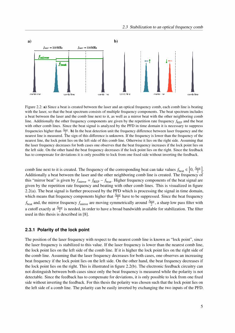
Figure 2.2: a) Since a beat is created between the laser and an optical frequency comb, each comb line is beatingwith the laser, so that the beat spectrum consists of multiple frequency components. The beat spectrum includesa beat between the laser and the comb line next to it, as well as a mirror beat with the other neighboring combline. Additionally the other frequency components are given by the repetition rate frequency fREP and the beatwith other comb lines. Since the beat signal is analyzed by the PFD in time domain it is necessary to suppressfrequencies higher than fREP

2 . b) In the beat detection unit the frequency difference between laser frequency and thenearest line is measured. The sign of this difference is unknown. If the frequency is lower than the frequency of thenearest line, the lock point lies on the left side of this comb line. Otherwise it lies on the right side. Assuming thatthe laser frequency decreases for both cases one observes that the beat frequency increases if the lock point lies onthe left side. On the other hand the beat frequency decreases if the lock point lies on the right. Since the feedbackhas to compensate for deviations it is only possible to lock from one fixed side without inverting the feedback.

comb line next to it is created. The frequency of the corresponding beat can take values fbeat ∈[0, fREP

2

].

Additionally a beat between the laser and the other neighboring comb line is created. The frequency ofthis “mirror beat” is given by fmirror = fREP − fbeat. Higher frequency components of the beat signal aregiven by the repetition rate frequency and beating with other comb lines. This is visualized in figure2.2(a). The beat signal is further processed by the PFD which is processing the signal in time domain,which means that frequency components higher that fREP

2 have to be suppressed. Since the beat frequencyfbeat and, the mirror frequency fmirror are moving symmetrically around fREP

2 , a sharp low pass filter witha cutoff exactly at fREP

2 is needed, in order to have a broad bandwidth available for stabilization. The filterused in this thesis is described in [8].

2.3.1 Polarity of the lock point

The position of the laser frequency with respect to the nearest comb line is known as “lock point”, sincethe laser frequency is stabilized to this value. If the laser frequency is lower than the nearest comb line,the lock point lies on the left side of the comb line. If it is higher the lock point lies on the right side ofthe comb line. Assuming that the laser frequency decreases for both cases, one observes an increasingbeat frequency if the lock point lies on the left side. On the other hand, the beat frequency decreases ifthe lock point lies on the right. This is illustrated in figure 2.2(b). The electronic feedback circuitry cannot distinguish between both cases since only the beat frequency is measured while the polarity is notdetectable. Since the feedback has to compensate for deviations, it is only possible to lock from one fixedside without inverting the feedback. For this thesis the polarity was chosen such that the lock point lies onthe left side of a comb line. The polarity can be easily inverted by exchanging the two inputs of the PFD.

5

Chapter 2 Phase-frequency stabilization

2.4 Optical Setup

The optical setup used for beat detection is shown in figure 2.3. The laser is firstly coupled into a fiber inorder to make a replacement of the laser easier if necessary. The light is then split with a polarizing beamsplitter (PBS), and send into two separate arms. The PBS reflects or transmits the light depending onits polarization. By rotating the polarization of the incoming laser beam with a half wave plate (HWP),it is possible to adjust the power ratio between the two arms. Both arms consists of an acusto opticalmodulator (AOM) in double pass configuration. Inside the AOM a piezo driven by a radio frequency(RF) modulates density fluctuations in a crystal. The density wave travels through the crystal and createsa moving grating. The laser frequency is thereby effectively shifted by the applied radio frequency. Thelaser beam is retro reflected, after passing the AOM once and thus it passes the AOM again. Hereby afrequency shift of two times the AOM driving frequency is achieved. AOM 1 shifts the frequency ofthe light that is used for beat detection. AOM 2 shifts the light that is send to the experiment and is alsoused for intensity stabilization. For further description the two arms will be denoted “beat arm” and“experiment arm”, respectively. The light in the beat arm is superimposed with the comb light for beatdetection. A grating is used to filter out the part of the comb spectrum that is close to 770 nm.

2.5 Electronic Setup

The electronic setup is shown in figure 2.4. A DC-block (DCB) is used to remove the DC part fromthe photo diode signal. A high pass filter (HPF) and a low pass filter (LPF) are used to shape the beatsignal. The LPF shows a sharp cutoff at 120 MHz. The purpose of this filter is to suppress frequencieshigher than fREP

2 = 125 MHz. The HPF is used for supporting the DC-block and has a cutoff frequency of20 MHz. The filter design is explained in detail in [8]. A power splitter (PS) divides the signal so thatone part can be monitored with a spectrum analyzer, while the other part is send to the PFD. The PFDcompares the beat signal with the stable RF reference provided by a direct digital synthesizer (DDS) andprovides two error signal outputs. The low frequency (LF) output is connected to a lock box in order toapply feedback to the piezo inside the laser. The high frequency output (HF) is connected to a loop filter,which then applies feedback to the diode current for phase locking. The reference frequency provided bythe DDS (AD9954) is controlled by an mbed microcontroller (mbed LPC1768). The DDS is thereforeprogrammed by the mbed via a serial peripheral interface (SPI). The driving frequency for AOM 1 isgenerated by a voltage controlled oscillator (VCO). This VCO is also controlled by the mbed via ananalog line. The mbed controller itself has an analog input, which can be read out by arbitrary programsin order to control the setup. These programs are explained in [8].

2.5.1 Lock box

The lock box is used for frequency stabilization of the laser. It contains a PI controller, which processesthe LF error signal. The output of such a PI controller consists of a proportional and an integral part as itis shown in equation (2.4).

c(t) = P · e(t) + I ·∫ t

0e(τ)dτ (2.4)

Here e(t) denoted the LF error signal at time t. P and I are adjustable coefficients which control theproportional and integral gain of the controller. The output c(t) is the signal that is sent to the piezo tocorrect the frequency deviations.

6

2.5 Electronic Setup

AOM double pass 2

/4

770nm

AOM double pass 1

/4

cavity

/2

Pol./2/4

Pol./2/4

Figure 2.3: Optical setup consisting of the laser, two AOM double pass configurations and the beat detection unit.The light is firstly split into the two separate AOM double pass configurations which shift the frequency of the lightby an applied radio frequency. AOM 1 shifts the light that is used for beat detection. AOM 2 shifts the frequency ofthe light that is sent to the experiment and is also used for intensity stabilization. The optical frequency is illustratedusing different colors. Yellow corresponds to the original laser frequency. Blue indicates a frequency shifted byAOM 1 and purple indicates a shift by AOM 2. In the beat detection unit the laser light is superimposed with thecomb light. A grating is used to filter out the part of the comb spectrum that is close to 770 nm.

PFD

LF

HPF

PS

Loop

�lter

Lock

Box

HF

DDS

LPF

to experiment

AOM double pass 1

Spec. Analyser

comb

VCO

Analog Input

mbed

DCB

AOM double pass 2

current modulation

to piezo

Figure 2.4: Simplified optical and electronic setup. The laser light is first shifted by AOM 1 and then superimposedwith the comb light. The beat signal is detected with a fast photo diode. The output of the photo diode is amplifiedand shaped with multiple electronic filters. A power splitter sends part of the signal to a spectrum analyzer formonitoring purpose. The other half is connected to the PFD where it is compared to some stable reference providedby a DDS. The PFD provides two error signal outputs. The low frequency signal (LF) is connected to a lock boxthat applies feedback to the laser piezo. The high frequency signal (HF) is sent into a loop filter in order to applyfeedback to the diode current. The driving frequency for AOM 1 is generated by a VCO that is controlled by anmbed microcontroller via an analog line. The mbed also controlles the frequency provided by the DDS. Therefore,the mbed and the DDS communicate via a serial peripheral interface.

7

Chapter 2 Phase-frequency stabilization

beat

reference

HF

LF

LPF

digitalization PFD

a)

b)

Figure 2.5: a) Schematic overview over the PFD. b) Logic diagram of the MC100EP140. One can see that the chipis sensitive to rising edges on the reference (R) and beat (FB) input. The two output signals up (U) and down (D)are either in the high (H) or the low (L) state and change between these states as shown. Figure taken from the datasheet of the MC100EP140 [9].

2.5.2 Loop filter

The loop filter consists of a low pass filter, a lead filter, a voltage divider and some protection circuitry.The low pass filter is used to filter frequencies that are to high for correction purposes. The leak filtershifts the phase of the signal to make sure that negative feedback is applied to the current modulation,such that phase deviations are suppressed and not amplified. A voltage divider is used to control the gain.Zener diodes and a DC blocking capacitor are inserted at the output of the loop filter to limit the currentsent into the laser.

2.6 Phase frequency discriminator

In order to achieve a phase-frequency lock of an IFL, one has to apply proper feedback to the piezo andthe diode current. This feedback has to compensate for deviations of the frequency and the phase. Thesedeviations are detected and quantified by a PFD, that was developed by Professor Marco Prevedelli,Università di Bologna. The PFD circuitry can be divided into 3 parts. The sinusoidal input is firstdigitized by an AD96687 comparator. The digitized signals are then fed into the phase-frequency detectorMC100EP140. This chip has two differential outputs whose behavior is described by the logic diagramin figure 2.5(b). The behavior of the differential “Up” and “Down” output is analyzed with two functiongenerators, which were both locked to the 10 MHz reference signal from an atomic clock. The functiongenerators were configured to have the same frequency but a phase difference. From the logic diagramone can see that in this case the PFD is oscillating between two states. Either between 1 and 2 or between2 and 3. In both cases one of the differential outputs is fixed at its low level, while the other one isoscillating between high and low level. The duty cycle of this output corresponds to the phase differenceof the input signals. This is shown in figure 2.6(a,b). The differential output signals of the MC100EP140are then smoothed with a low pass filter, in order to convert the duty cycle to a DC voltage. The cutoff

frequency of this first order low pass filter is at 33.9 MHz. The difference between the differential outputsafter low pass filtering is then amplified with a AD8129 differential amplifier. The output of this amplifierserves as HF error signal. The LF error signal is derived from that by filtering with a first order low pass

8

2.6 Phase frequency discriminator

that has its cutoff frequency at 3.4 MHz. The PFD translates a phase difference into a proportional DCvoltage. This voltage has boundaries which means, that for phase differences higher than some ∆ϕmax theoutput voltage saturates. It follows from this that the “phase span” which can be covered by the PFD issmaller than 2π. Experimentally it turned out that the phase span of the PFD is of the order of 10 % of 2π.

2.6.1 RF leakage

In the previous section, it has been explained that the PFD stores the phase information in the duty cycleof two differential outputs. This duty cycle is then converted into a DC voltage by a low pass filter. If onewants to detect a phase difference for signals which have a frequency that is close to the cutoff frequencyof the smoothing low pass, one observes “RF leakage”. In this case the duty cycle is not convertedproperly to a DC voltage and the error signal is not constant although the phase difference is kept constant.This can be seen in figure 2.6(c). For a constant phase deviation between the two input signals of thePFD the error signal should be flat. If the error signal is affected by RF leakage, one can measure anoscillation of the error signal which is frequency dependent. The amplitude of the error signal oscillationis shown in figure 2.6(d) as function of frequency. By increasing the capacitance of the low pass filter, itis possible to reduce its cutoff frequency, since this is given by fcutoff = 1

2πRC . Here R is the resistance ofthe low pass and C the capacitance. Figure 2.6(d) shows that one can reduce the influence of RF leakageby changing the cutoff frequency of the smoothing low pass. Without additional capacitors it is possibleto establish a stable phase lock for beat frequencies higher than 60 MHz. By adding a 22 pF capacitor tothe existing 4.7 pF capacitor the cutoff frequency is changed to 6 MHz. With this changes it is possibleto establish a stable phase lock for frequencies higher than 40 MHz. With additional capacitors, it isstill not possible to lock at beat frequencies lower than 40 MHz, although the AC amplitude of the errorsignal is lower than the former limit at 60 MHz without additional capacitors. This cannot be explainedwith RF leakage and remains unknown. For further analysis one should lock at the frequency dependantamplification of the differential amplifier.

9

Chapter 2 Phase-frequency stabilization

Figure 2.6: a)+b) Phase information is stored in the duty cycle of the differential outputs of the PFD. Two functiongenerators (green,purple), both locked to the atomic clock, were configured to have the same frequency but a phasedifference. One can see that the duty cycle of the differential up (yellow) and down (blue) output carries the phaseinformation. The phase difference between 0 and 2π is proportionally mapped to a duty cycle between 0 and 1. c)RF leakage for different cutoff frequencies of the smoothing low pass filter. d) AC amplitude of the error signalas function of RF frequency for constant phase deviations. The AC amplitude is measured for different cutoff

frequencies of the smoothing low pass filter. Without any additional capacitor it is possible to establish a stablephase lock for frequencies higher than 60 MHz. The dashed line indicates the AC amplitude of the error signal forthis frequency without changing the cutoff of the low pass.

10

CHAPTER 3

Continuous frequency tuning of a phase-lockedlaser

This chapter is devoted to the techniques used for scanning the laser frequency continuously over severalhundreds of MHz, requiring scanning across multiple comb lines [10–12]. This demands eloquenttechniques while crossing a comb line in order to maintain phase stability of the lock. In this regard 3different scanning schemes are explained and compared. The implementation of one of these schemes isdescribed. All schemes have in common that the optical frequency of the locked laser is set in particularby the frequency difference between the laser frequency and the nearest comb line, since the beat signalof these is used for stabilization. For further description the relative position of the laser frequency withthe respect to the nearest comb line is denoted as “lock point”. The need of a lock point jump is explainedwithin this chapter and the optimization of this process is described.

3.1 Moving the lock point

If the reference signal for the PFD is changed, an error signal is generated which indicates the deviationbetween beat frequency and its new set point. Feedback to the laser piezo and diode current is generatedfrom this error signal by the lock box and the loop filter. This feedback changes the optical laser frequencysuch that the new beat frequency matches the reference frequency. Hereby the laser can be scanned. Inthe ideal case, the scannable bandwidth is given by fREP

2 = 125 MHz. For beat frequencies close to fREP2 ,

the lock might be disturbed by the mirror beat, due to competition between beat frequency and mirrorfrequency. The maximum beat frequency is limited by the frequency response of the low pass filter. Asharp cutoff at fREP

2 is needed in order to allow locking at beat frequencies close to fREP2 . With the used

low pass filter a stable lock is possible for frequencies up to 115 MHz. On the low frequency side one islimited by the ESC. Experimentally it turned out that the PFD is not working properly for frequencieslower than 40 MHz as described in section 2.6. A scannable bandwidth of 75 MHz is obtained fromthese boundaries. If the laser needs to be scanned over broader regions where locking is not directlypossible due to the discussed issues, one has to insert a frequency shifting element either in the beat armor the experiment arm. In this case the laser frequency at the output of the locking setup is shifted withrespect to the lock point. Hereby it is possible to keep the lock point in the valid region while the outputfrequency can be tuned continuously.

11

Chapter 3 Continuous frequency tuning of a phase-locked laser

3.2 Scanning schemes

For this project an AOM was used in double pass configuration such that the optical laser frequencyis shifted by two times the AOM driving frequency. The setup includes a double pass in the beat arm(AOM 1) and the experiment arm (AOM 2) as it is shown in figure 2.4. Both AOMs are used in positivefirst order double pass and shift the laser frequency as shown in figure 3.1(a). With this configuration,different scanning schemes are possible which will be explained next. These schemes have their ownadvantages and drawbacks and are compared in this section.

3.2.1 AOM 1 based scanning

In this scheme, the driving frequency of AOM 1 is changed [11]. This causes a change of the opticalfrequency used for beat detection and consequently a change of the beat frequency. The deviation fromthe reference frequency causes feedback to the laser to bring the lock point back to the set point, such thatthe laser frequency is effectively scanned. By changing the frequency of AOM 1 it is possible to keepthe lock point in the valid region while the laser frequency can be scanned continuously. The drivingfrequency of AOM 2 can be set to a constant value. It is then used for intensity stabilization only. Ifone wants to scan the laser frequency upwards, one can first reduce the reference frequency such thatthe lock point comes closer to the comb line. Since the lock point lies on the left side of a comb line, areduction of the reference signal causes an increasing laser frequency. If the laser needs to be scannedfurther, one has to reduce the driving frequency of AOM 1. Since the lock point is fixed via the feedbackthe laser frequency is increased that way. Once the laser has been scanned for fREP = 250 MHz one hasto simultaneously reset the reference frequency fref and the AOM 1 driving frequency faom1 such thatthe lock point jumps to the next comb line, preparing it for another round of action. During this jumpthe comb line used for beat detection changes but the optical output frequency remains constant. For asmooth jump of the lock point without disturbing the laser, one has to make sure that equation 3.1 holds.(

fref,max − fref,min

)+ 2 ·

(faom,max − faom,min

)= fREP (3.1)

Here fref,min and faom,min denote the reference frequency and the AOM driving frequency before the lockpoint jump. The frequencies after the lock point jump are denoted by fref,max and faom,max. This orderchanges if the laser frequency is scanned downwards. If equation (3.1) is not fulfilled precisely thelaser frequency is changed during a jump of the lock point. For optimization of the jump it is possibleto monitor the error signal during the jump. If the error signal remains flat, the laser frequency inthe experiment arm is not changed independently of the processes in AOM 1. The lock point jump isexplained in detail in section 3.3. The signals used for scanning the laser are shown in figure 3.1(b).

3.2.2 AOM 2 based scanning

In this scheme the driving frequency of AOM 1 is kept constant but the AOM 2 frequency is changed inorder to scan the laser [10, 12]. The laser can be scanned again by changing the reference. In order toincrease the laser frequency over the “forbidden region”, one has to increase the driving frequency ofAOM 2. The intensity stabilization is again done with AOM 2. The AOM in the beat arm is not used inthis scheme. An advantage of this AOM 2 based scanning is that only one AOM is necessary for scanningand intensity stabilization. Scanning with AOM 2 is also faster since it does not dependent on the lockingbandwidth. A serious drawback is that the output frequency of the setup is scanned continuously whilethe laser itself is not following continuously. That means that during the lock point jump the laserfrequency has to be changed by 2 ·

(faom,max − faom,min

). This is shown in figure 3.1(c). The execution

12

3.2 Scanning schemes

0

50

100

[MH

z]

150

200

250

[MH

z]

0 125 250 375 500

optical frequency with respect to an arbitrary comb line [MHz]

500

0

500

[MH

z]

0

50

100

[MH

z]

150

200

250

[MH

z]

0 125 250 375 500

optical frequency with respect to an arbitrary comb line [MHz]

500

0

500

[MH

z]

a) b)

0

50

100

[MH

z]

150

200

250

[MH

z]

0 125 250 375 500

optical frequency with respect to an arbitrary comb line [MHz]

500

0

500[M

Hz]

c) d)

Figure 3.1: a) The laser light (yellow) is split and send into two separate AOM double pass configurations. AOM1 (orange) shifts the light in the beat arm that is used as lock point (blue). AOM 2 (red) shifts the light in theexperiment arm (purple). In the beat detection unit a beat signal is measured between the light in the beat arm andthe frequency comb. This beat signal (green) is used for locking b) AOM 1 based scanning. The laser frequencyis scanned by changing either the reference frequency or the driving frequency of AOM 1. AOM 2 is kept ata constant frequency and is used only for intensity stabilization. At some point the reference and the AOM 1frequency have to be reset, so that the lock point jumps to the next comb line. c) AOM2 based scanning. The laseris scanned by changing the reference frequency or the AOM 2 driving frequency. d) Polarity change scheme. Thelaser can be locked from both sides to a comb line, since the polarity is inverted properly. Scanning the laser overcomb lines includes an AOM in the beat arm.

time of such a frequency step of the laser frequency is limited by the bandwidth of the piezo inside theIFL. It follows, that a lock point jump in this scheme is slower and less stable, since the laser frequencyhas to follow the previous scan. The frequency step could be implemented by charging capacitors thatare then “fired” into the laser[13]. Optimization of the jump in this scheme is more complicated sinceneither the beat signal nor the error signal can be used as feedback.

3.2.3 Polarity scheme

In this scheme the polarity of the feedback is invert-able such that the laser can be locked from both sidesto a comb line. An AOM in either the beat arm or the experiment arm is nevertheless necessary becauselocking does not work close to comb lines and in the middle between two comb lines. In figure 3.1(c) anAOM in the beat arm is assumed. Two jumps per 250 MHz scan are needed, since the forbidden regionnext to comb lines have to be bypassed as well as the region close to the polarity change. The errorsignal can be used as feedback for optimizing the jump. For this project AOM 1 based scanning wasimplemented. An AOM in the experiment arm was also installed in order to make a intensity stabilizationof the laser beam possible. This AOM 2 is also useful for faster “out of loop” tuning of the laser frequency.The only disadvantage of this setup is, that it binds more optical and electronic components.

13

Chapter 3 Continuous frequency tuning of a phase-locked laser

3.3 Lockpoint jump

During the lock point jump the driving frequency of the AOM in the beat arm as well as the referencesignal provided by the DDS is changed. This is shown in figure 3.2(a). The optical laser frequency shouldnot be changed during this process. Therefore, it is important that the laser does not undergo feedbackwhich would change the frequency or phase. Consequently, it is important that the error signal does notcause such a feedback. During the jump the optical frequency on the photo diode is changed due to thechange of the AOM driving frequency. Consequently, the efficiency of the AOM is also changed duringthe AOM ramp [8]. Due to this efficiency ramp the optical power on the photo diode is changed whichcauses a change of the DC part of the photo diode signal. On the rising edge of the AOM efficiency theDC part of the photo diode signal increases. The derivative of the DC increase passes the DC block andcauses the amplifiers to saturate so that no meaningful beat signal is obtained during the jump. Thisis shown in figure 3.3(b). It is therefore not possible to have active feedback on the laser within the“jumptime”. In order to avoid disturbing the laser, it is necessary to adjust the reference frequency fromthe DDS in a way that the PFD generates a error signal with smallest possible amplitude.

The AOM driving frequency is generated by a VCO which is controlled via an analog output line ofthe mbed microcontroller. The analog line is amplified for technical reason. In order to fulfill equation3.1, one has to precisely adjust the input value of the digital to analog converter such that the frequenciesare generated properly. For this optimization process it is convenient to monitor the error signal duringthe jump. If the values are not properly set, one observes a saturation of the error signal which meansthat the laser frequency is changed. This can be seen in figure 3.2(b). By adjusting the frequencies of thereference signal and the AOM driving signal it was possible to reduce the time within the error signalsaturates down to 13 µs. This short saturation occurred due to missing synchronization of the referencefrequency jump and the AOM frequency jump. To synchronize the jump a certain frequency ramp ispreprogrammed in the DDS board. This ramp is executed on a trigger event which allows a precisesynchronization with the change of the AOM driving frequency. The frequency ramp includes a certain“waiting time”, before changes are applied, in order to get the mbed enough time to change the AOMfrequency. A schematic overview over the steps executed during the jump is shown in 3.2(c). Duringthe jump the reference frequency is increased and decreased step wise in order to keep the error signaloscillating around zero. In figure 3.3(a) one can see a measurement of the error signal, the beat signaland the reference signal from the DDS during the lock point jump. The frequency of the reference signalis changed during the jump in order to keep the error signal as flat as possible.

3.4 Optical frequency synthesizer

The frequency comb spectrum consists of multiple equally spaced comb lines and thus provides afrequency ruler which can be used for synthesizing optical frequencies with high precision [14]. Theoptical laser frequency at the output of the locking setup is defined by the position of the lock point andthe AOM frequencies. If the comb line number used for locking is known, it is possible to synthesizean arbitrary optical frequency by adjusting the reference frequency and the AOM frequencies. For thiscalibration procedure it is necessary to measure the optical frequency with a wavemeter. The comb linenumber n which is used for locking can then be calculated by formula (3.2). Therefore it is necessarythat the optical frequency is known with a precision better than fREP

2 = 125 MHz.

n · fREP + fCEO = fout − 2 · faom2 + 2 · faom1︸ ︷︷ ︸lock point

+ fbeat (3.2)

14

3.4 Optical frequency synthesizer

With a known lock point it is then possible to synthesize optical frequencies by adjusting the AOMdriving frequencies and the reference frequency for the PFD. The accuracy of the synthesized opticalfrequency depends on the accuracy of the VCO and the DDS frequency. Since all this frequencies occurlinear in formula (3.2) the uncertainties can be simply summed up taking the prefactor 2 into account.Note that the carrier envelope offset frequency fCEO might be negative.

Figure 3.2: a) During the lock point jump the AOM driving frequency (orange) and the reference frequency (green)are changed. That causes the lock point (blue) to jump to the next comb line while the laser frequency (yellow) andthe output frequency (purple) are not changed. b) Measurements of the error signal during the lock point jump.If the frequencies are not properly chosen such that equation 3.1 holds, one observes that the laser frequency ischanged unintentionally, which can be seen on the error signal. c) Schematics of the program executed by thembed controller during the lock point jump.

Figure 3.3: a) Measurement of the error signal (blue), the beat signal (green) and the reference signal (yellow)during the lock point jump. The beat signal vanishes during the jump due to a change in the AOM efficiency whichcauses the amplifiers to saturate. The reference signal from the DDS is adjusted in a way that the PFD generatesan error signal with smallest possible amplitude in order to avoid a change of the optical laser frequency. Theamplitude of the error signal is smaller that its saturation level, which is indicated by the grey box. b) Zoomedversion of the same signals.

15

CHAPTER 4

Analysing lock stability

For a quantitative study of the phase and frequency stability of a locked laser, one can use differenttechniques which analyze either electronic “in-loop signals” that are used for stabilization or “out ofloop” signals that are not used for feedback generation. The coarse and long term frequency stability isanalyzed with a wavemeter that records the optical frequency of the stabilized laser beam as function oftime. The available frequency resolution is of the order of a few MHz, which is limited by the resolutionof the wavemeter. When the laser is referenced to an optical frequency comb, a wavemeter measurementis useful to verify that the laser is always locked to the same predetermined comb line. If the combline that is used as lock reference changes unintentionally, the wavemeter measures a frequency step offREP = 250 MHz. The gain parameters of the servo lock loop are adjusted to avoid any unintended lockpoint jump due to external disturbances. Another intuitive way for in loop lock stability analysis wouldbe to monitoring the error signal since this signal is quantifying phase and frequency deviations. Theresolution of phase and frequency deviations in this case depends on the ESC and is usually very precisecompared to the other possible measurements. Also the in-loop beat signal that is used for stabilizationcan be analyzed in terms of its power spectral density. This spectrum usually shows a typical feature ofthe central carrier peak at the desired lock point and two servo bumps also called sidebands. The controlbandwidth can be estimated from the position of these sidebands with respect to the central carrier. Theresidual phase noise can be estimated from this spectrum by determining the power in the sidebands. Forthis project it is of interest to analyze the phase and frequency stability during the lock point jump andalso during certain frequency ramps of the laser. Especially the phase and frequency stability during thelock point jump has to be verified. In order to analyze the lock point jump a wavemeter measurement isnot useful, since the available wavemeter resolution is not precise enough. It is also not possible to usethe error signal for a stability verifying analysis, since this signal was already used for optimization. Inaddition to that it is not possible to use the in-loop beat spectrum, due to the saturation of the amplifiersduring the jump. Because of this saturation the beat signal is not meaningful during the jump, as it wasexplained in more detail in section 3.3. In order to analyze the stability of the phase and the frequency amore elaborated analysis is required. This analysis is based on another out of loop beat signal betweenthe stabilized laser beam and the frequency comb. For an estimation of the frequency stability from thissignal one has to measure the frequency and phase of the beat signal as function of time. This approachis described further in section 4.2.

17

Chapter 4 Analysing lock stability

Figure 4.1: Beat signal measured with a spectrum analyzer while the laser was locked. The frequency resolution isset to 10 kHz and the spectrum is averaged over 10 traces. The central peak at 90 MHz is surrounded by two servobumps at a relative position of ±1.1 MHz

4.1 In-loop beat signal

This section deals with the analysis of the beat signal that is used for locking. As shown in fiure 2.4 apower splitter divides the beat signal so that a spectrum can be measured with a spectrum analyzer whilethe laser is locked. A measured beat spectrum for this locked case is shown in figure 4.1. It is obtainedthat 99.06 % of the power lies inside the carrier peak. The carrier peak at exactly 90 MHz is surroundedby two servo bumps at a relative position of ±1.1 MHz. This frequency difference can be interpreted aslocking bandwidth. The area under the servo bumps represents phase noise of the beat signal with respectto the central carrier peak.

4.2 Time frequency analysis

For further analysis of the phase and frequency stability one can take the stabilized laser beam andcreate another beat signal with the frequency comb. This second out-of-loop beat signal is not used forcorrection purpose and thus a more reliable out of loop analysis can be done by analyzing this beat signal.For this project the beat signal was measured in time domain with a 2.5 GS s−1 oscilloscope. Traces wererecorded for a time span of 2 ms.

Assuming that the laser frequency is properly stabilized, a constant beat frequency is measured.Therefore it is important to obtain the beat frequency as function of time. In order do obtain thecorresponding spectra one has to multiply the signal with a window function before calculating theFourier spectrum. The window function is zero except for some region of interest, such that the timedependency can be analyzed by moving the window over the signal. The influence of the window functionis explained in more detail in section 4.2.2.

18

4.2 Time frequency analysis

4.2.1 Frequency resolution

The number of frequency bins returned from the FFT algorithm determines the resolution of the spectrum.This bin width ∆ ffft can be calculated from the sampling rate fsample and the number of data points N byequation (4.1).

∆ ffft =fsample

N(4.1)

In order to reduce the bin width “zero padding” can be used. This technique adds a series of zeros tothe time domain signal such that the number of data points N is effectively increased. No frequencycomponents of interest are appended, since only a DC part of frequency 0 Hz is added. In order to analyzethe influence of zero padding a simulated signal was used consisting of two monochromatic sinusoidalswith frequencies 50 MHz and 50.5 MHz. White noise with a σ of 10 % of the signal amplitude was added.Figure 4.2 shows the influence of zero padding for this signal. In 4.2(a) the signal shown in 4.2(d) isanalyzed directly without adding zeros. In 4.2(b) zeros are added such that 50 % of the analyzed windowcontains zeros. In 4.2(c) the analyzed window contains 99 % zeros. One can see that the number of datapoints lying in the 10 MHz span increases. In spite of the small frequency bin width one does not see twoclear peaks at the expected frequencies of 50 MHz and 50.5 MHz. Although the FFT resolution is goodenough, the “signal resolution” ∆ fsignal is not. The signal resolution is according to equation (4.2) theinverse time span of the time domain data and represents the minimum detectable frequency difference.

∆ fsignal =1T

(4.2)

If the signal is not zero padded, the signal resolution ∆ fsignal and the frequency bin width ∆ ffft are equal.Zero padding is useful to clarify the exact position of a maximum within a peak. Figures 4.2(d-f) showthe influence of different window length. For spectrum 4.2(d) a 2 µs window was used, that was filledwith zeros to reach a 200 µs span. For spectrum 4.2(e) 20 µs time domain data was used and 180 µsof zeros were added in order to have the same bin width as in 4.2(d). In 4.2(f) a 200 µs window wasused and no zeros were added. For all these spectra the frequency bin width is 5 kHz, while the signalresolution changes between 500 kHz for 4.2(d), 50 kHz for 4.2(e) and 5 kHz for 4.2(f), respectively. Fromequation (4.2) it becomes clear, that the signal resolution can be improved by increasing the amount oftime domain data used for each spectrum. One has to decide whether a good time or frequency resolutionis necessary since the product of time uncertainty ∆t = T and frequency uncertainty ∆ fsignal is fixed,according to equation (4.3).

∆ fsignal · ∆t = 1 (4.3)

For this project a monochromatic frequency is expected and thus the maximum of the frequency dis-tribution is of interest. The position of the maximum is independent of the width of the correspondingpeak and thus the position of the maximum is mainly defined by the bin width and not be the signalresolution. Therefore it is possible to use a “fine” time resolution and increase the frequency resolutionwith zero padding. Different window functions can be used for analyzing the frequency dependence.There influence on the calculated spectrum is discussed in the next section.

19

Chapter 4 Analysing lock stability

Figure 4.2: A signal consisting of two monochromatic frequencies at 50 MHz and 50.5 MHz is simulated. Theinfluence of zero padding and window length is analyzed. a) The window length was set to cover a time span of2 µs and thus a frequency resolution fsignal of 500 kHz is possible. For figures a) and b) zero padding is used toreduce the bin width of the calculated fourier spectrum. The analyzed signal contains 50 % zeros in b) and 99 %zeros in c). In d) the frequency resolution is again 500 kHz. By increasing the amount of time domain data that isused for calculation of the spectra it is possible to improve the frequency resolution. The frequency resolution is50 kHz in e) and 5 kHz in f). Zero padding is used such that all spectra are calculated with a bin width of 5 kHz. g)2 µs span of the time domain data.

20

4.2 Time frequency analysis

Figure 4.3: A 10 MHz sinusoidal is sampled with 2.5 GS s−1 for a window length of 20 µs. Zero padding is usedto reduce the fft bin width to 500 Hz. The signal shown in d) is analyzed with different window functions. Thewindow function and the calculated spectra are shown. One can see that all windows induce certain features aroundthe expected carrier peak. The decay of these features depends on the choice of the window function as well as thewidth of the central carrier. a) Rectangular window. b) Tukey window. c) Hann window.

4.2.2 Window function

Let s(t) be the beat signal, W(t) the window function and F[s](ω)(t) the spectrum of signal s(t) associatedwith time t. If W(t) is normalized such that

∫ ∞−∞

W(t) dt = 1 one can calculate the spectrum according toequation (4.4). For choosing a window function it is important to notice that the calculated spectrumconsists of a convolution of the beat fourier spectrum with the fourier spectrum of the window function.This is shown in figure 4.3.

F[s](ω)(t) =

∫ ∞

−∞

s(τ)W(τ − t) exp (−iωτ) dτ (4.4)

A monochromatic frequency of 10 MHz was simulated and Gaussian noise with a σ of 50 % the signalamplitude was added. The signal was analyzed with different window functions. The window functionsand their corresponding spectra are shown in figure 4.3. The window length is 20 µs in all cases whichcorresponds to a signal resolution of 50 kHz. Zero padding is used to reach a bin width of 500 Hz. Infigure 4.3(a) one can see, that a rectangular window function creates several widely spreading featuresaround the expected carrier. One one hand, the width of this carrier increases when the window functionis changed to a Tukey-window (4.3(b)) or a Hann-window (4.3(c)). On the other hand one observes thatthe amplitude of the features decays faster for such a window. For predicting the form of these featuresone has to calculate the fourier transformation of the used window function, since the spectrum consistsof a convolution of the signal spectrum with the window spectrum.

21

Chapter 4 Analysing lock stability

4.3 Out-of-loop beat spectrum

The out-of-loop beat spectrum between stabilized laser and frequency comb provides information aboutthe lock quality. It is useful in terms of analyzing the stability of a static lock point as well as analyzingcertain modulations in frequency or phase of the laser. Firstly the influence of different AOM frequenciesis analyzed. Next a frequency modulation is applied to the laser and a proof of concept is given byanalyzing the out-of-loop beat spectrum.

4.3.1 mbed noise

As explained in section 2.5 the AOM driving frequency is generated via a VCO which is controlled byan analog line from the mbed microcontroller. Experimentally it turned out that this analog output isdisturbed by a 1 kHz noise. The laser follows this noise, since the frequency is smaller that the lockingbandwidth. Consequently one can see this kind of low1 frequency noise on the error signal but not on thein-loop beat spectrum, that is used for stabilization. On the out-of-loop beat spectrum this is neverthelessvisible. This is shown in figure 4.4(c). In figure 4.4(a) the out-of-loop beat spectrum is shown over a 2 mstime span. The time resolution is set to 10 µs, which is reasonable since this is a longer time than theinverse control bandwidth. With this a signal resolution of 0.1 MHz is obtained. Exploiting zero paddinga bin width of 25 kHz is used. In figure 4.4(a1) the control voltage to the VCO is almost zero whichmeans, that the AOM is driven with 150 MHz. For figures 4.4(a2,a3) the AOM is driven with 200 MHzand 250 MHz, respectively. This corresponds to control voltages of 5 V and 10 V. From the comparisonof figures 4.4(a1-a3) one can see that the noise amplitude increases with an increasing output voltage ofthe VCO control port. The same shaped noise was visible directly on the VCO control port as one cansee in figure 4.5. In figure 4.4(b) the maximum of the frequency distribution is shown for each time step.By fitting a constant frequency ffit to this trace it is possible to quantify the amount of noise with thevalue χ2, that is defined in equation (4.5).

χ2=

N∑i

(fi − ffit

)2 (4.5)

4.3.2 Lock point jump

The laser frequency should remain constant during the lock point jump. In section 3.3 it has beenexplained that the error signal was monitored in order to optimize this process. By analyzing the out-of-loop spectrum it is possible to verify the expected stability during this process. The jump process isfinished within 3 µs. For a time resolution of ∆t = 3 µs a signal frequency resolution of ∆ fsignal = 333 kHzis possible.

4.3.3 Frequency modulation

For this measurement the AOM driving frequency as well as the reference frequency were generatedby two function generators which where locked to a 10 MHz signal from an atomic clock. The AOMfrequency was set to constant value, while the reference frequency was modulated using another functiongenerator. The amplitude of this modulation was set to 1 MHz and the modulation frequency was chosento be 5 kHz. The error signal, the in-loop beat signal and the out-of-loop beat signal where recorded

1 low compared to the locking bandwidth

22

4.3 Out-of-loop beat spectrum

Figure 4.4: a) Spectra obtained for different AOM driving frequencies. Due to the noise on the analog controlport a effective frequency modulation is applied to the AOM driving frequency. The amplitude of this unintendedmodulation increases with an increase of the control voltage. In a.1) the control voltage is set to 10 V. For a.2) anda.3) the voltage is set to 5 V and 0.06 V. b) The maximum of the spectra from a) is shown. By fitting a constantfrequency it is possible to quantify the amount of noise via the χ2 value. c) Due to the unintended frequencymodulation the the beat frequency used for stabilizing the laser is also modulated. Since the frequency of this noiseis 1 kHz which is lower than the control bandwidth, the feedback corrects these deviations such that the in loopbeat frequency remains constant. This causes a modulation of the laser frequency in the experiment arm which isvisible in the out of loop spectrum. c.1) In loop beat spectrum. c.2) Out of loop beat spectrum. c.3) Error signal.

23

Chapter 4 Analysing lock stability

with 2.5 GS s−1. Figure 4.7 shows the calculated beat spectra, as well as the recorded error signal. Onthe in-loop spectrum it is clearly visible that the reference frequency is modulated. On the out of loopspectrum it is clearly visible that the laser frequency follows this modulation. This result proves that atime-frequency analysis of the out-of-loop beat spectrum is useful in terms of analyzing the response ofthe laser to an applied modulation.

Figure 4.5: The analog output port of the mbed shows a certain noise of frequency 1 kHz. For this measurementthe analog output port was connected to an oscilloscope and the AC coupled signal was recorded over 2 ms. Theshape of this signal locks very similar to the detected frequency noise analyzed in section 4.3.1.

24

4.3 Out-of-loop beat spectrum

Figure 4.6: a) Maximum of the in loop spectrum during the lock point jump. As explained in section 3.3 thereference frequency is changed during the lock point jump. The step from 105 MHz to 44 MHz can be seen. b)The spectrum of the out of loop beat signal is shown with a signal frequency resolution of 100 kHz. With thisresolution no influence of the lock point jump is visible. c) Error signal.

Figure 4.7: For this measurement a frequency modulation was applied to the reference frequency. The amplitude ofthis modulation was set to 1 MHz and the modulation frequency was sets to 5 kHz. a) In loop beat signal. b) Outof loop beat signal. c) Error signal.

25

CHAPTER 5

Summary and Outlook

In this thesis, I presented a phase and frequency lock of an interference filter laser to an optical frequencycomb. The stabilization is done by creating a beat signal between both lasers which oscillates withthe frequency difference of both laser beams after reasonable low pass filtering (see chapter 2). Sincethe reference laser is assumed to be stable, fluctuations of the beat frequency and phase are relatedto corresponding changes of the laser that has to be stabilized. These fluctuations are quantified by aerror signal circuit (ESC) [1, 4, 5] which electronically compares the beat signal with a radio frequencyprovided by a direct digital synthesizer (DDS). The working principle of the ESC is explained as wellas the optical and electronic setup used for locking. The working principle of a frequency comb isintroduced briefly and difficulties of a lock referenced to an optical frequency comb are pointed out. Thefrequency components of the beat spectrum are explained and the need for proper electronic filters isderived from that [8].

Scanning the laser frequency continuously over several hundreds of MHz requires scanning acrossmultiple comb lines. This demands eloquent techniques while crossing a comb line in order to maintainphase stability of the lock. In chapter 3 the need of a frequency shifting element is derived from that.Different frequency tuning schemes are explained that make use of the frequency shift by an acustooptical modulator [10, 12]. These schemes allow a continuous tuning of the laser frequency over multiplecomb lines and have their own advantages and drawbacks. They have in common that the laser frequencycan be tuned by adjusting the reference frequency of the ESC. Hereby, the setpoint for the frequencydifference between the laser and the nearest comb line is changed causing a change of the laser frequencyby the feedback loop, since the comb spectrum is fixed. The presented schemes differ in terms of theAOM position and the applied driving frequencies. For a continuous scan of the laser frequency it ispossible to shift either the light that is used for beat detection [11] or the useful light at the output ofthe locking setup [10, 12]. In both cases, a change of the respective AOM driving frequency causes achange of the laser frequency. This driving frequency has to be reset at some point, which is denotedas “lock point jump”. During this lock point jump the comb line used for locking changes, while thelaser frequency should remain constant. The optimization of this process is explained also in chapter3. One useful application for the implemented lock scheme is an optical frequency synthesizer [14]. Aserial command line interface based on a microcontroller was implemented to set the synthesized opticalfrequency by automatically generating the necessary control variables for the locking scheme.

In Chapter 4, the analysis of the lock stability is discussed based on a measured spectrum of the “inloop” beat signal. It is obtained that 99.06 % of the power lies inside the central carrier. A lockingbandwidth of 1.1 MHz is estimated from the position of the servo bumps. A further analysis obtains thetemporal behavior of the “out of loop” beat signal between the stabilized laser and the frequency comb

27

Chapter 5 Summary and Outlook

by means of time frequency analysis. This analysis is based on the Fourier transform of the time domainsignal which is multiplied by a moving window function [15]. The influence of the window function tothe observed spectra as well as the available time resolution ∆t and frequency resolution ∆ f is explained.Both resolutions are not independent since the product is fixed, which can be expressed by ∆ f · ∆t = 1.This analysis approach is finally applied to several out of loop and in loop spectra. Noise generated bythe analog output of the mbed microcontroller is precisely quantified and the frequency stability duringthe lock point jump is verified. In addition a programmed modulation of the laser frequency is verified.

Outlook For this project, the driving frequency for the in loop AOM is generated by a voltage controlledoscillator that is steered by an analog output line of the mbed microcontroller. This output is carryinga 1 kHz noise signal which could not be removed during this project. However, the intrinsic frequencyinstability of the VCO would limit the lock accuracy even in the absence of control voltage noise. Inorder to improve the lock stability the corresponding frequency could be generated via a DDS. Such asetup would enable us to optimize the lock point jump further to shorter time scales limited only by therise time of the AOM instead of the slew rate of the analog mbed output. An additional advantage is,that a frequency step could be send during the lock point jump which is currently impossible due to thelimited slew rate. As a consequence the AOM frequency is swept causing a change of the transmittedpower during the lock point jump which leads to a saturation of the photo diode amplifiers. This processis explained in more detail in section 3.3. Due to this saturation it is not possible to actively stabilize thelaser during the 3 µs jump time.

The investigation of the maximum tuning rate of the laser frequency is of interest in quantum opticsexperiments. So far tuning rates up to 480 MHz s−1 have been demonstrated [8]. The maximum tuningrate could be optimized and compared for the 3 different scanning schemes explained in section 3.2.

In order to analyze not only the frequency stability of the lock, but also the phase stability one couldanalyze the position of the zero crossings of the out of loop beat signal. By analyzing the time of a zerocrossing as function of its number it is possible to interpret the fluctuations around a constant slope asphase noise [16].

For autonomous operation as an optical frequency synthesizer is is of importance to qualify the lockstability in real time by the software on the microcontroller. If indications of multi mode operation of thelaser are detected the microcontroller could compensate this via the laser diode current modulation portof the laser controller. Such a second feedback is expected to strongly increase the bandwidth availablefor frequency tuning.

28

Bibliography

[1] U. Schünemann et al., Simple scheme for tunable frequency offset locking of two lasers,Review of Scientific Instruments 70 (1999) 242, url: https://doi.org/10.1063/1.1149573(cit. on pp. 1, 3, 27).

[2] E. D. Black, An introduction to Pound–Drever–Hall laser frequency stabilization,American Journal of Physics 69 (2001) 79, url: https://doi.org/10.1119/1.1286663(cit. on p. 1).

[3] M. Hohn, Frequenzstabilisierung eines Diodenlasers mittels Doppler-freier Spektroskopie aneiner Erbium-Hohlkathodenlampe (Bachelorarbeit IAP), (2017) (cit. on p. 1).

[4] G. Ritt et al., Laser frequency offset locking using a side of filter technique,Applied Physics B 79 (2004) 363, url: https://doi.org/10.1007/s00340-004-1559-6(cit. on pp. 1, 3, 27).

[5] J. Hughes and C. Fertig, A widely tunable laser frequency offset lock with digital counting,Review of Scientific Instruments 79 (2008) 103104,url: https://doi.org/10.1063/1.2999544 (cit. on pp. 1, 3, 27).

[6] Nobelprize.org., The Nobel Prize in Physics 2005, (), Nobel Media AB 2014. Web. 15 Aug 2017.,url: http://www.nobelprize.org/nobel_prizes/physics/laureates/2005/(cit. on p. 1).

[7] M. S. GmbH, FC1500-250-ULN User Manual, (2016) (cit. on p. 4).

[8] L. Ahlheit, Frequenzvariable Phasenstabilisierung eines Diodenlasers auf einen optischenFrequenzkamm (Bachelorarbeit IAP), (2017) (cit. on pp. 5, 6, 14, 27, 28).

[9] MC100EP140 datasheet, (2017),url: https://www.onsemi.com/pub/Collateral/MC100EP140-D.PDF (cit. on p. 8).

[10] T. Sala et al., Wide-bandwidth phase lock between a CW laser and a frequency comb based on afeed-forward configuration, Optics Letters 37 (2012) 2592,url: https://doi.org/10.1364/ol.37.002592 (cit. on pp. 11, 12, 27).

[11] W. Gunton, M. Semczuk and K. W. Madison, Method for independent and continuous tuning of Nlasers phase-locked to the same frequency comb, Optics Letters 40 (2015) 4372,url: https://doi.org/10.1364/ol.40.004372 (cit. on pp. 11, 12, 27).

[12] J. D. Jost, J. L. Hall and J. Ye,Continuously tunable, precise, single frequency optical signal generator,Opt. Express 10 (2002) 515,url: http://www.opticsexpress.org/abstract.cfm?URI=oe-10-12-515(cit. on pp. 11, 12, 27).

29

Bibliography

[13] T. Fordell et al., Frequency-comb-referenced tunable diode laser spectroscopy and laserstabilization applied to laser cooling, Appl. Opt. 53 (2014) 7476,url: http://ao.osa.org/abstract.cfm?URI=ao-53-31-7476 (cit. on p. 13).

[14] R. Holzwarth et al., Optical Frequency Synthesizer for Precision Spectroscopy,Physical Review Letters 85 (2000) (cit. on pp. 14, 27).

[15] P. D. Welch, The Use of Fast Fourier Transformation for the Estimation of Power Spectra: AMethod Based on Time Averaging Over Short, Modified Periodograms,IEEE Trans. Audio and Electroacust. AU-15 (1967) 70 (cit. on p. 28).

[16] M. Schiemangk et al., Accurate frequency noise measurement of free-running lasers,Applied Optics 53 (2014) 7138, url: https://doi.org/10.1364/ao.53.007138(cit. on p. 28).

30