An Optimal Constraint Programming Approach to the Open

___________________________

An Optimal Constraint Programming Approach to the Open-Shop Problem

Arnaud Malapert Hadrien Cambazard Christelle Guéret Narendra Jussien André Langevin Louis-Martin Rousseau

June 2009

CIRRELT-2009-25


Arnaud Malapert1,2,3,*, Hadrien Cambazard4, Christelle Guéret2, Narendra Jussien2, André Langevin1,3, Louis-Martin Rousseau1,3

1 Interuniversity Research Centre on Enterprise Networks, Logistics and Transportation

(CIRRELT) 2 École des Mines de Nantes, 4, rue Alfred Kastler, B.P. 20722, 44307 NANTES Cedex 3,

France 3 Département de mathématiques et génie industriel, École Polytechnique de Montréal, C.P.

6079, succursale Centre-ville, Montréal, Canada H3C 3A7 4 Department of Computer Science, University College Cork, Western Rd Cork, Co Cork, Ireland

Abstract. This paper presents an optimal constraint programming approach for the Open-

Shop problem, which integrates recent constraint propagation and branching techniques

with new upper bound heuristics for the Open-Shop problem. Randomized restart policies

combined with nogood recording allow to search diversification and learning from restarts.

This approach closed all remaining problems of the Brucker et al. and Guéret and Prins

benchmarks with cpu times that are orders of magnitude lower than the best known

metaheuristics.

Keywords. Production-scheduling, open-shop, computers-computer science, artificial

intelligence, constraint programming, randomization and restart.

Acknowledgements. The corresponding author wish to thank Laboratoire d’informatique

de Nantes-Atlantique (LINA), Institut de Recherche en Communications et Cybernétique

de Nantes (IRCCyN), École des Mines de Nantes (EMN), Centre interuniversitaire de

recherche sur les réseaux d’entreprise, la logistique et le transport (CIRRELT), and

Laboratoire Quosséça.

Results and views expressed in this publication are the sole responsibility of the authors and do not necessarily reflect those of CIRRELT. Les résultats et opinions contenus dans cette publication ne reflètent pas nécessairement la position du CIRRELT et n'engagent pas sa responsabilité. _____________________________

* Corresponding author: [email protected] Dépôt légal – Bibliothèque et Archives nationales du Québec, Bibliothèque et Archives Canada, 2009

© Copyright Malapert, Cambazard, Guéret, Jussien, Langevin, Rousseau and CIRRELT, 2009

1. Introduction

Open-Shop problems are at the core of many scheduling problems involving unary resourcessuch as Job-Shop or Flow-Shop problems, which have received an important amount of at-tention due to their wide range of applications. Among the many techniques proposed in theliterature, Constraint Programming (CP) belongs to the most successful ones. We proposein this paper a constraint programming approach for the Open-Shop problem based on themost recent methods developed for scheduling problems in CP. Our approach relies on theuse of strong propagation mechanisms of the unary resource global constraint and temporalconstraint network but also reasoning dedicated to the minimization of the makespan suchas the forbidden intervals method. Our main contribution is to show that randomization andrestart strategies combined with strong propagation and scheduling heuristics can lead toa very efficient approach for solving Open-Shop problems. The proposed solving techniqueoutperforms the other approaches published so far on a wide range of benchmarks.

This paper is organized as follows. We first recall the main techniques for solving Open-Shop problem based both on complete algorithms and local search approaches in section2. Secondly, section 3 gives an overview of the state-of-the-art methods used in ConstraintProgramming for Open-Shop problems. Section 4 describes our approach relying on ran-domization and restarting strategies with nogood recording and section 5 presents the ex-perimental results we obtained. It investigates in more detail the effect of each componentof the algorithm as well as its parameters.

2. Problem Definition and State of the Art

In the Open-Shop problem (OSP), a set J of n jobs, consisting each of m tasks (or operations),must be processed on a set M of m machines. The processing times are given by a matrixP : m × n, in which pij ≥ 0 is the processing time of task Tij ∈ T of job Jj, to be doneon machine Mi. The tasks of a job can be processed in any order, but only one at a time.Similarly, a machine can process only one task at a time. We consider the construction ofnon-preemptive schedules of minimal makespan Cmax, which is NP-Hard for m ≥ 3 (seeGonzalez and Sahni, 1976).Let denote by LJ

k =∑

i∈M pik the load of job k ∈ J and by LMk =

∑j∈J pkj the load of

a machine k ∈ M . The maximum load over every machine and every job CLBmax is a lower

bound for the OSP.CLB

max = max(LJk |k ∈ J ∪ LM

k |k ∈M)

We review the main exact approaches on Open-Shop problems and the most recent localsearch techniques giving the best-known results.

Only a few exact methods for the OSP have been published so far. The first one (Bruckeret al., 1996) is based on the resolution of a one-machine problem with positive and negativetime-lags. The second one (Brucker et al., 1997) consists in fixing precedences on the criticalpath of heuristic solutions computed at each node. Although that last method is efficient,some problems of Taillard (1993) benchmark from size 7×7 remained unsolved. Gueret et al.(2000) proposed an intelligent backtracking technique applied to the Brucker et al. branchingscheme. When a contradiction is raised during search, instead of systematically backtracking


CIRRELT-2009-25 1

to the previous decision (chronological backtracking), the algorithm analyses the reasonsfor the contradiction to avoid questioning decisions that are not related to the failure andbacktracks to a more relevant choice point. This approach significantly reduces the number ofbacktracks but can be two times slower than the initial version in each node. More recently,Dorndorf et al. (2001) improved the Brucker et al. algorithm by using CP techniques. Insteadof analyzing and improving the search strategies, they focused on constraint propagationtechniques for reducing the search space. The algorithm was the first to solve many probleminstances to optimality in a short amount of time. However, some problems of Taillard’sbenchmark from size 15 × 15 remained unsolved as well as some of Brucker et al. (1997)instances from size 7× 7.

At the same time, many metaheuristic algorithms have been developed in the last decadeto solve the OSP. The most recent and successful metaheuristics are : Ant Colony Optimiza-tion(ACO – Blum, 2005), Particle Swarm Optimization (PSO – Sha and Hsu, 2008) andGenetic Algorithm (GA – Prins, 2000). The basic component of ACO is a probabilistic solu-tion construction mechanism. Due to its constructive nature, ACO can be regarded as a treesearch method. Based on this observation, Blum (2005) hybridizes the solution constructionmechanism of ACO with Beam Search (BS). BS algorithms are incomplete derivatives ofBranch-and-Bound algorithms. It is an approximate method where a partial assignment isonly extended in a restricted number of ways (this limit is called the beam width). Beam-ACO improves on the results obtained by the current best standard ACO algorithms. PSOis a population-based optimization algorithm, where each particle is an individual solution,and the swarm is composed of many particles. Sha and Hsu (2008) modify the representationof particle position, particle movement, and particle velocity to better fit to the OSP. Theyobtain many new best-known solutions of the benchmark problems. Genetic Algorithms area particular class of evolutionary algorithms that use techniques inspired by evolutionarybiology such as mutation, selection, and crossover. Prins (2000) presents several specializedOSP genetic algorithms with two key-features: a population in which each individual has adistinct makespan, and a special procedure which reorders every new chromosome.

Finally, there are many heuristic methods that quickly provide good solutions to theOSP. Most of them are constructive heuristics and belong to three main families: prior-ity dispatching rules, matching algorithms (see Gueret, 1997) and insertion and appendingprocedures combined with beam search (see Brasel et al., 1993).

3. The Constraint Programming Model

In this section, we present our constraint programming model to tackle specifically Open-Shop problems. First, we briefly present basic CP notions, especially in the schedulingcontext before discussing propagation and branching techniques. At each step, we presentstate-of-the-art methods, explain our choice and our contribution.

Constraint programming techniques have been widely used to solve scheduling problems.A Constraint Satisfaction Problem (CSP) consists of a set V of variables defined by a cor-responding set of possible values (the domain D) and a set C of constraints. A solutionof the problem is an assignment of a value to each variable such that all constraints aresimultaneously satisfied. Constraints are handled through a propagation mechanism which


CIRRELT-2009-25 2

allows the reduction of the domains of variables and the pruning of the search tree. Thepropagation mechanism coupled with a backtracking scheme allows the search space to beexplored in a complete way. Scheduling is probably one of the most successful areas for CPthanks to specialized global constraints which allow modelling resource limitations such asthe unary resource or cumulative global constraints (see Beldiceanu and Demassey, 2006).

Constraint Programming models in scheduling usually represent a non-preemptive taskTij by a triplet of non-negative integer variables (sij, pij, eij) denoting the start, durationand end of the task so that sij + pij = eij. In Open-Shop problems, the duration pij isknown in advance and is a constant. The head of a task, estij = inf(sij), denotes the earliestpossible starting date of the task whereas the tail lctij = sup(eij) is the latest completiontime. The Open-Shop problem states that a single task of a machine or job can be processedat any given time. These constraints are modeled by the mean of the well known unaryresource global constraint. Finally, temporal constraints such as precedences between tasksare used in the decision process. We now give more details on these constraints and theirimplementations.

3.1. Unary Resource

A unary resource global constraint, also called Disjunctive, models a resource of unit capacity.A unary resource constraint holds if all the tasks of a collection that have a duration strictlygreater than 0 do not overlap. One unary resource constraint is stated for each job and eachmachine. First, we present state-of-the-art propagation algorithms for the unary resourceconstraint. We also take advantage of the propagation to compute a dynamic lower bound ofthe makespan. Finally, in addition to these methods, a technique called forbidden intervalsis used to improve pruning.

Unary Resource Propagation Let T denote a set of tasks sharing an unary resourceand Ω denote a subset of T . We consider the three following propagation rules :

Not First/Not Last (NF/NL): This rule determines if task i cannot be scheduled after orbefore a set of tasks Ω. In other words, it implies that i cannot be last or first in theset Ω ∪ i. In that case, at least one task from the set must be scheduled after (resp.before) activity i and the tail (resp. head) of i can be updated accordingly.

Detectable Precedence (DP): A precedence i ≺ j (see section 3.2) is called detectable, if itcan be discovered only by comparing the time bounds of its two tasks. Heads andtails of each task can then be updated more accurately by the knowledge of all thepredecessors or successors.

Edge Finding (EF): This filtering technique determines that some task must be executedfirst or last in a set Ω ⊆ T . It is the counterpart of the NF/NL rule.

Several propagation algorithms (Carlier and Pinson, 1994; Caseau and Laburthe, 1995; Bap-tiste and Le Pape, 1996; Vilım, 2004) exist for these rules and the best of them have acomplexity of O(n log(n)).All the previous rules rely on the computation of the earliest completion time (ECTΩ) of


CIRRELT-2009-25 3

a set Ω ⊆ T of tasks. By denoting estΩ = minTij∈Ωestij, the earliest completion time isdefined as follow:

ECTΩ = maxestΩ′ +∑Ω′

pij, Ω′ ⊆ Ω (1)

We choose the implementation proposed by Vilım (2004) that relies on two efficient datastructures : Θ-tree and Θ-Λ-tree. These structures are based on a balanced binary tree andallow a quick computation of ECTΩ for a given set of tasks Ω, especially at each addition orremoval of a task in the set.

The filtering algorithms of a constraint reach a local fixpoint when they can no longerreduce domains of its variables. The order in which the filtering algorithms are applied affectsthe total runtime, although it does not influence the resulting local fixpoint. Vilım (2004)proposed a filtering algorithm where each rule reaches its fixpoint in a main propagation loopwhich is executed until no update is performed. We have a main propagation loop whereeach rule is executed only once. We order the rules to minimize the number of sorts requiredby the data structures and to perform all updates on heads before tails.

Makespan Propagation We also take advantage of the computation of ECTΩ to estimatea lower bound of the makespan ECTOSP . In fact, the earliest completion time of a machineMi (resp. a job Jj) is given by the value of ECTMi

(resp. ECTJj). Let R = Jjj∈[1,m] ∪

Mii∈[1,n] denote the set of all unary resources, then the makespan is greater than themaximum of the earliest completion time among all resources and is given by the formulaECTOSP = maxΩ∈RECTΩ.

Forbidden Intervals Forbidden intervals are a specialized filtering technique for OSP withminimal makespan. Forbidden intervals are intervals in which in an optimal solution, taskscan neither start nor end. Heads and tails can be strengthened based on this informationduring search. When the head of a task is in such an interval, it can be increased to theupper bound of the interval. This technique has been proposed by Gueret and Prins (1998)and the computation of forbidden intervals is based on the resolution of m + n Subset-SumProblems (Kellerer et al., 2004). The Subset-Sum Problem has an O(d×n) complexity whered is the capacity of the knapsack, i.e. the maximal makespan. The Subset-Sum problemsare solved at the beginning of the search and heads and tails are updated in a constant time.

3.2. Temporal Constraints

This section deals with the problem of managing quantitative temporal networks withoutdisjunctive constraints. The problem is known as the Simple Temporal Problem (STP). Aswe only deal with precedence constraint network, we specialized the procedure and datastructures for incremental constraint posting and propagation algorithms.

Simple Temporal Problem A Simple Temporal Problem is defined in Dechter et al.(1991) and involves a set of temporal integer variables X1, . . . , Xn and a set of constraintsaij ≤ Xj −Xi ≤ bij, where bij ≥ aij ≥ 0. A solution of the STP is an assignment of thevariables such that every temporal constraint is satisfied. A directed graph G = (V, E) is


CIRRELT-2009-25 4

associated with the problem. The set of nodes V represents the set of variables X1, . . . , Xnand the set of edges E represents the set of temporal constraint. A couple of edges, (j, i)labeled with weight −aij and (i, j) labeled with weight bij are associated with each temporalconstraints aij ≤ Xj − Xi ≤ bij. Dechter et al. (1991) proved that a Simple TemporalProblem is consistent if and only if G does not have negative cycles.

Cesta and Oddi (1996) proposed algorithms to manage temporal information that : (a) al-low dynamic changes of the constraint set for both posting and retraction (b) exploit thetemporal constraint network for incremental propagation and cycle detection. Dechter (2003)reviewed most properties and algorithms for the STP. Unfortunately, most of the propertiesand algorithms supposed that no unary resource is involved.

Precedence Constraints Network In an Open-Shop problem, let Tij ≺ Tkl denote aprecedence constraint, i.e. a temporal constraint such that pij ≤ skl−sij ≤ +∞. Of course,precedences could be handled by simply adding the corresponding elementary constraints tothe solver and by propagating them independently. But, we take advantage of previous workon STP to gain in efficiency and flexibility. First, we slightly modify G, then we adaptposting and retraction and propose a new algorithm to perform propagation.

The set of nodes V now represents the set of tasks. Two fictitious tasks Tstart and Tend

referring to the starting and ending tasks of the schedule, are added to that set. An arc isadded in E between two tasks Tij and Tkl if Tij precedes Tkl (Tij ≺ Tkl). Initially, the onlyarcs of E are the ones originating at node Tstart or ending at node Tend. For example, Figure1 represents G for a 3×3 OSP instance with a set of six precedence constraints where initialedges are dotted and precedence edges are plain. The makespan Cmax of a schedule is thelength of a longest path between Tstart and Tend, a critical path.

initial edges

T11

T31

T21 T22

T32

T13

T33

T23

T12

Tstart Tend

Figure 1: Representation of the precedence constraint network G associated with a 3 × 3OSP instance and a set of six precedence constraints.

The precedence constraint network is consistent if and only if it does not have any cycle.So, G is a Directed Acyclic Graph (DAG). Furthermore, an implied precedence can be easilydetected when it is implied by the bounds of the tasks but it is not necessarily the casefor transitive precedences. Indeed, precedence constraints satisfy the triangular inequalityTij ≺ Tpq ∧ Tpq ≺ Tkl ⇒ Tij ≺ Tkl. So, if an arc (Tij, Tkl) is transitive, i.e. Tij and Tkl

are connected by a path in E\(Tij, Tkl), then the precedence Tij ≺ Tkl is already implied.A branching strategy over precedences should avoid branching on transitive or satisfiedprecedences.

The incremental algorithm based on the Bellman-Ford algorithms for the Single SourceShortest Path Problem proposed by Cesta and Oddi (1996) has a O(|V | × |E|) complexity.


CIRRELT-2009-25 5

Since G is a directed acyclic graph, our incremental algorithm, based on the Dynamic Bell-man algorithm for the Single Source Longest Path problem (Gondran and Minoux, 1984),has a linear complexity.

Network Representation We choose to design a specific and centralized data structureto represent the precedence constraint network. Typically, cycles and transitive precedencescan be detected much faster with a centralized data structure dealing with the network ofprecedences. Furthermore, propagation of a set of precedences can be done in linear timewhereas a bad ordering of awakes in the propagation loop can lead in the worst case toquadratic time before reaching the fixpoint.

The structure can efficiently handle arc insertions/removals and is restorable upon back-tracking, i.e., it maintains a stack to record when a change is performed on the graph. Cycleand transitive arc detections have a constant time complexity as we maintain the transitiveclosure of G. Frigioni et al. (2001) proposed an implementation for maintaining the transi-tive closure information in a directed graph. Their approach requires O(n) amortized timefor a sequence of insertions and deletions. In addition, we also maintain a topological orderwith the simple and efficient algorithm proposed by Pearce and Kelly (2006). In fact, thetransitive closure information reduces the overall complexity to maintain a topological order.To give an example, suppose that the precedence T12 ≺ T22 has just been added in Figure1. Then, a choice point would be created since this precedence is not transitive and did notintroduce a cycle.

Then, the transitive closure of the vertices T11 and T12 is updated. The transitive closureof T12 is updated from Tend to T22, T32, T33, Tend. Similarly, the transitive closure of T11 isupdated to T12, T22, T32, T33, Tend. Assume a topological order O1, the updated topologicalorder after addition of T12 ≺ T22 is indicated below as O2.

(T21, T22, T31, T32, T33, T13, T23, T11, T12) (O1)

(T21, T31, T11, T12, T22, T32, T33, T13, T23) (O2)

Branching strategies exploit the data structure to avoid branching on transitive prece-dence or create cycle in the network. Furthermore, the data structure is used to speeduppropagation. Indeed, to update the head and tail of Tij according to G, the longest path be-tween Tstart and Tij, as well as Tij and Tend is computed. All shortest paths originating fromTstart and ending at Tend are computed in a linear time with the Dynamic Bellman algorithmfor the Single Source Longest Path problem (Gondran and Minoux, 1984). As a topologicalorder is an input of the algorithm, our implementation avoids redundant computations bymaintaining a dynamic topological order. Last, at each propagation, the algorithm considersonly a subgraph of G where the head or the tail of the tasks has changed since the last call.

To summarize, the precedence constraints network is represented by a dynamic and back-trackable directed acyclic graph in which arc insertions and deletions can be done in lineartime. The propagation is done in linear time by an algorithm based on the Dynamic Bellmanalgorithm for the Single Source Longest Path problem.


CIRRELT-2009-25 6

3.3. Symmetry Breaking

Many constraint satisfaction problems contain symmetries making many solutions equiva-lent. Symmetry breaking techniques avoid redundant search effort by trying to ensure thatwhenever a partial assignment is shown to be inconsistent, no symmetric assignment is evertried.

In our case, a solution of the OSP can be reversed considering the last task of a machineas the first, the second to last task as the second and so on. This symmetric counterpart ofany solution is also a solution for the OSP. Once the algorithm has proved that one orderingof the tasks was suboptimal, it is unnecessary to check the reverse ordering. Breaking thissymmetry can be done in two manners by picking: (a) any task Tij and impose, a priori,

that it starts in the left part of the schedule sij ≤⌈

Tend−pij

2

⌉; (b) any pair of tasks , Tij and

Tkl, belonging to the same job or same machine, and impose, a priori, that Tij ends beforeTkl starts, i.e. Tij ≺ Tkl. We will evaluate these alternatives and denote by START theconstraint (a) where we select the task with the longest processing time, and by PREC theconstraint (b) where we select the pair of tasks with the longest cumulated processing times.

3.4. Branching Scheme

Branching strategies in scheduling can be divided in two main families: assigning startingdates or fixing precedences.

In the first category, the most well known is referred to as setTimes (Le Pape et al.,1994) and is an incomplete branching scheme. At each node, it selects a task from a set ofunscheduled and selectable tasks, creates a choice point and schedules the selected task atits earliest starting time. Upon backtracking, it labels the task that was scheduled at theconsidered choice point as not selectable as long as its earliest start has not changed. Thisbranching scheme is generic but it does not allow the efficient solution of large problems.

The second category consists in fixing precedences between tasks. In OSP contexts, theblock branching of Brucker et al. (1997) (denoted as Block) is based on the computation ofa heuristic solution in each node to decide the precedences to enforce. The tasks along thecritical path of this heuristic solution are selected and precedences are stated to questionthe current critical path. This branching scheme can fix many precedences at the sametime while remaining complete. Beck et al. (1997) proposed a simpler binary branchingscheme (denoted as Profile) where two critical tasks sharing the same unary resource areordered. This heuristic, based on the probabilistic profile of the tasks, determines the mostconstrained resources and tasks. At each node, the resource and the time point with themaximum contention are identified, then a pair of tasks that rely most on this resource atthis time point are selected (it is also ensured that the two tasks are not already connectedby a path of temporal constraints). Once the pair of tasks has been chosen, the order ofthe precedence has to be decided. For that purpose, we retain one of the three randomizedvalue-ordering heuristics of Beck et al. (1997) : centroid. The centroid is a real deterministicfunction of the domain and is computed for the two critical tasks. The centroid of a taskis the point that divides its probabilistic profile equally. We commit the sequence whichpreserves the ordering of the centroids of the two tasks. If the centroids are at the sameposition, a random ordering is chosen.


CIRRELT-2009-25 7

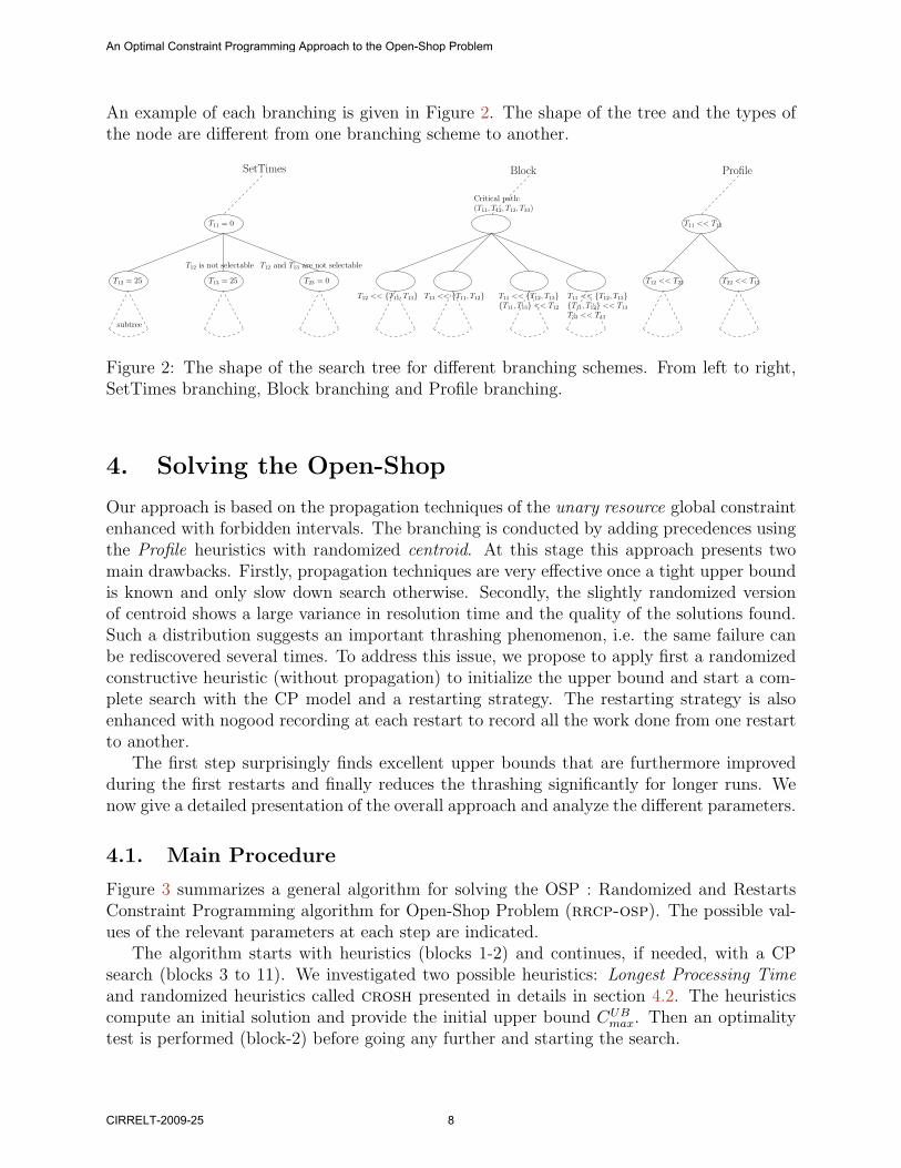
An example of each branching is given in Figure 2. The shape of the tree and the types ofthe node are different from one branching scheme to another.

T11 = 0

T12 = 25 T13 = 25 T23 = 0

T12 is not selectable

(T11, T12, T13, T33)Critical path:

T12 << T11, T13 T13 << T11, T12 T11 << T12, T13T11, T13 << T12

T11 << T12, T13T11, T12 << T13

T33 << T13

T11 << T12

T12 << T22 T22 << T12

ProfileSetTimes

subtree

T12 and T13 are not selectable

Block

Figure 2: The shape of the search tree for different branching schemes. From left to right,SetTimes branching, Block branching and Profile branching.

4. Solving the Open-Shop

Our approach is based on the propagation techniques of the unary resource global constraintenhanced with forbidden intervals. The branching is conducted by adding precedences usingthe Profile heuristics with randomized centroid. At this stage this approach presents twomain drawbacks. Firstly, propagation techniques are very effective once a tight upper boundis known and only slow down search otherwise. Secondly, the slightly randomized versionof centroid shows a large variance in resolution time and the quality of the solutions found.Such a distribution suggests an important thrashing phenomenon, i.e. the same failure canbe rediscovered several times. To address this issue, we propose to apply first a randomizedconstructive heuristic (without propagation) to initialize the upper bound and start a com-plete search with the CP model and a restarting strategy. The restarting strategy is alsoenhanced with nogood recording at each restart to record all the work done from one restartto another.

The first step surprisingly finds excellent upper bounds that are furthermore improvedduring the first restarts and finally reduces the thrashing significantly for longer runs. Wenow give a detailed presentation of the overall approach and analyze the different parameters.

4.1. Main Procedure

Figure 3 summarizes a general algorithm for solving the OSP : Randomized and RestartsConstraint Programming algorithm for Open-Shop Problem (rrcp-osp). The possible val-ues of the relevant parameters at each step are indicated.

The algorithm starts with heuristics (blocks 1-2) and continues, if needed, with a CPsearch (blocks 3 to 11). We investigated two possible heuristics: Longest Processing Timeand randomized heuristics called crosh presented in details in section 4.2. The heuristicscompute an initial solution and provide the initial upper bound CUB

max. Then an optimalitytest is performed (block-2) before going any further and starting the search.


CIRRELT-2009-25 8

In block 3 of the figure, the CP model is created and various components are initialized. Asymmetry breaking constraint is added (block 4) and three possibilities have been analyzed:no symmetry breaking (OFF), restricting the starting date of the longest task (START) orfixing the precedence between the two tasks of the same job or machine with the longestprocessing times (PREC). Section 3.3 discussed these choices in details.

initialize nogood store if any

endstart

1

2

3

4

6

5

7 8

9

10

11

yes

no

yes

no

yes

no

yesno

yes

no

restart

yes

no

initialize variable domains

initialize constraints store

(disjunctive, precedence, forbidden intervals).

define variables

propagate constraints

solutionfound?

set dynamic cut: TRUEcut: eend < CUB

max

set dynamic cut: FALSE

fathomed?all branches

backtrack

dynamiccut?

inconsistencyproven ?

CUBmax = CLB

max ?

add symmetry breaking constraint

compute CUBmax, CLB

max

CROSH(Literation, Ltime)alternatives : LPT,

branches: Tij << Tkl, Tkl << Tij

Branching

select critical tasks : (TijTkl)should restart?

WALSH(s, g), FIXED(s)alternatives : OFF, LUBY(s, g),

alternatives : OFF,NOGOOD

alternatives : RANDOM, CENTROIDrandomized value-ordering heuristic

alternatives : OFF, START, PREC

Figure 3: General outline of rrcp-osp. Ellipses are initial and final states. Rectangles areprocedures or actions. Diamonds are if-else conditions. Dashed rectangles are labels.

The generic loop of the algorithm is contained between blocks 5 and 11. After propagationand domain reduction (block 5), we might have reached a solution, a contradiction or neitherof those two cases. If a solution is found, it is recorded and the new upper bound ofthe makespan is used to add a constraint as a dynamic cut that will be propagated upon


CIRRELT-2009-25 9

backtracking. If a failure is detected and all branches of the root node have been fathomed,then optimality of the last solution found is proved and the algorithm terminates. Otherwise,the algorithm backtracks. If the dynamic cut flag is set, then a propagation step is neededto take the new cut into account. Otherwise a branching step is needed but before that, weexamine the possibility to restart. Four different options for restarting have been analyzedin our study as shown on block 9 and discussed in more detail in section 4.3. In case ofrestarts we can extract nogoods (block 10) to avoid redundant work from one restart to thenext and keep track of the subproblems already proved suboptimal or infeasible.

If no restart is performed, then a search is undertaken using the Profile branching scheme(see section 3.4) in block 11. Branching divides the main problem into a set of exclusive andexhaustive subproblems by temporarily adding a precedence.

4.2. Initial Solution

Propagation techniques are very costly and only useful when applied with a good upperbound. Similarly, the branching technique is really sensitive to the quality of the upperbound as it relies on the demand curve of the resources. It is in practice very important toprovide a good upper bound at the root node in a small amount of time.

Priority Dispatching Rule (PDR) methods are classical and easy methods to construct anondelay schedule by repeatedly appending tasks to a partial schedule. A schedule is callednon-delay if no machine is left idle provided that is is possible to process some job. Startingwith an empty schedule, tasks are appended as follows: (a) determine the minimal head t0

of all unscheduled operations (at time t0, there exists both a free machine and an availablejob) (b) among all available tasks, choose one according to some priority dispatching rule.Common priority dispatching rules are Longest Processing Time (LPT) and Shortest Pro-cessing time (SPT). We do not consider SPT as Gueret (1997) experimentally proved thatLPT is the best classical heuristic. We prefer the PDR methods, which, beside from beinggeneric, simple and easy to implement, yield very good results experimentally (see section5.1.1).We based our Constructive Randomized Open-Shop Heuristics (CROSH) on this process,randomizing the selection of task at step (b) instead of following a dispatching rule. Algo-rithm 1 gives the details of such a heuristics.

It starts with the upper bound given by LPT (CLPTmax ) and attempts to improve it. As

each internal function has a constant time complexity, the overall complexity is given by thethree imbricated loops. 1, 2 and 3. The main loop 1 is executed at most Literation timesand the internal loop 2 and 3 are executed at most |Ut0| ≤ |T | = m× n times. The overallcomplexity of CROSH is O(m2×n2×Literation). Finally, if we choose the task of Ut0 with thelongest processing time instead of randomly (see line LPT), we obtain the LPT heuristics.

4.3. Restart Strategy

Restart policies are based on the following observation: the longer a backtracking searchalgorithm runs without finding a solution, the more likely it is that the algorithm is exploringa barren part of the search space. Initial choices made by the branching are both the leastinformed and the most important as they lead to the largest subtrees and the search can


CIRRELT-2009-25 10

hardly recover from early mistakes. This can lead to thrashing situations where failures aredue to a small subset of early choices but discovered much deeper in the tree over and overagain. An intelligent backtracking algorithm tries to compensate for the early mistakes ofthe heuristics by analyzing failures and identifying the choices responsible for the currentdead end situation. Restart strategies combined with randomization are another way to getrid of thrashing and bad initial choices.

As our technique is randomized, preliminary experiments reveal its great sensitivity tothrashing. Several runs could lead to very different results regarding the number of back-tracks and solution quality. It led us to investigate restart strategies and especially universalrestart strategies.

Algorithm 1: Constructive Randomized Open-Shop Heuristics (CROSH)

Data: T, J, M, CLBmax , CLPT

max , Ltime, Literation

Result: An upper bound on Cmax

UBCmax = CLPTmax ;

while checkLimits (Ltime,Literation) do1

/* no limit reached */Integer[] CTJ = Integer[n] ; // Job Completion TimeInteger[] CTM = Integer[m] ; // Machine Completion TimeCmax = 0 ; // current makespanU = T ; // set of unscheduled taskswhile U 6= ∅ do2

Ut0 = ∅ ; // set of selectable taskst0 =∞ ; // minimal head of unscheduled tasksforeach Tij ∈ U do3

estij = max(CTJ [i]), CTM [j]); // head of Tij

if estij < t0 then t0 = estij ; Ut0 = Tij;else if estij == t0 then Ut0 = Ut0 ∪ Tij;

LPT Ti0j0 = selectRandomly(Ut0) ;/* schedule the selected task */ect = t0 + pi0j0 ;U = U\Ti0j0;CTJ [i0] = ect; CTM [j0] = ect;Cmax = max(Cmax, ect);if Cmax ≥ UBCmax then break

if Cmax < UBCmaxthen

UBCmax = Cmax ;if UBCmax = CLB

max then break

return UBCmax;

Universal Restart Strategy. Let A(x) be a randomized algorithm of the Las Vegas type,which means that, on any input x, the output of A is always correct but its running timeTA(x) is a random variable. A universal restart strategy determines the length of any runfor all distributions on running time.

If the only feasible observation is the length of a run and there is no knowledge of therun-time distribution of the solver on the given instance, Luby et al. (1993) showed that the


CIRRELT-2009-25 11

universal schedule of cutoff values of the form

1, 1, 2, 1, 1, 2, 4, 1, 1, 2, 1, 1, 2, 4, 8, . . .

gives an expected time to solution that is within a log factor of that given by the best fixedcutoff, and that no universal schedule is better by more than a constant factor. The sequenceis often defined by adding a geometric factor r. By denoting sk = rk−1

r−1, the i-th term of the

sequence is defined as follows (r = 2 is the previous example):

∀i > 0 ti =

rk−1 if i = sk

ti−sk−1 if sk−1 + 1 ≤ i < sk

s = 1 and r = 3⇒ 1, 1, 1, 3, 1, 1, 1, 3, 1, 1, 1, 3, 9, . . .

Walsh (1999) suggests another universal strategy of the form s, sr, sr2, sr3, . . . growingexponentially, contrary to the Luby strategy which grows linearly. The two parameters thatwe consider are a scale factor s and a geometric factor r. The scale factor scales, or multiplies,each cutoff in a restart strategy. Wu and van Beek (2007) demonstrated both analytically andempirically the pitfalls of non-universal strategies and showed that parametrization of thestrategies improves performance while retaining any optimality and worst-case guarantees.As restarting seems a key component of those problems, we will evaluate the effects of thescale and geometric factors to identify a good restart strategy.

Nogood Recording from Restarts Our heuristics is only randomized when orderingtwo tasks to state a precedence and even in this case, the randomization only takes placewhen Centroid is unable to identify a good order. This slight randomization of the search isenough, as mentioned previously, to observe a huge variance in solution quality. However,in some cases, very few random choices are made and the same search tree is likely to beexplored from one restart to another. We apply a simple nogood recording technique similarto Lecoutre et al. (2007) to compensate for this drawback.

In our context, a nogood is defined with a current upper bound ub and corresponds toa set of precedences P , such that all solutions satisfying P have a makespan greater thanub. The same set P of precedences can be met from one restart to another. Recording Pcan avoid redundant work and provide more diversification across the restarts. We recordnogoods only when the search is about to restart (block 10 of Figure 3). At this point werecord all the nogoods representing the subtrees proven suboptimal following the idea ofLecoutre et al.. All the work accomplished during this step is therefore recorded and thesame part of the search tree will therefore not be explored in different runs. Only a linearnumber of nogoods is recorded at each restart.

Nogoods are propagated individually in Lecoutre et al. using watch literals techniques.We implemented the nogood store as a global constraint that achieves unit propagation onthe nogoods. Our implementation remains naive and could be improved based on watchliterals techniques. The number of nogoods remain quite small in practice as they are onlyrecorded at each restart and nogood propagation didn’t seem to be a bottleneck for efficiencyin our approach. We also remove nogoods that are subsumed by another one when addingall the nogoods coming from a new restart.


CIRRELT-2009-25 12

5. Computational Results

Three different sets of OSP benchmark instances are available in the literature. The firstset consists of 60 problem instances provided by Taillard (1993) (denoted by tai*) rangingfrom 16 operations (4 jobs and 4 machines) to 400 operations (20 jobs and 20 machines).Brucker et al. (1997) proposed also 52 difficult square OSP instances (denoted by j*) from 3jobs and 3 machines to 8 jobs and 8 machines. Finally, the last set is made of 80 benchmarkinstances provided by Gueret and Prins (1999) (denoted by GP*). The size of these instancesranges from 3 jobs and 3 machines to 10 jobs and 10 machines. All of the experiments wereperformed on a cluster with 84 machines running Linux, each node with 1 GB of RAM and a2.2 GHz processor. We perform several set of experiments in order to : (a) study the impactof the parameters and the various options in the algorithm (see section 5.1); (b) comparerrcp-osp with other state-of-the-art methods (see section 5.2).

5.1. Setting the Parameters of the Algorithm

We presented in section 4 various alternatives and parameters of our general algorithm rrcp-osp. We report here an experimental study of their importance for the algorithm and justifyexperimentally the choices made in the final set up of the algorithm.

5.1.1. Initial Solution

Two possibilities of heuristics were given in section 4.2 to compute an initial upper bound:crosh and LPT. In this section, we compare crosh and LPT and explain how the timelimit and the maximum number of iterations of crosh were chosen. First, we study thequality of the solution with regard to the number of iterations of crosh. crosh was runon each instance with a limit of 100000 iterations and a timeout of 30 seconds (20 runswere performed due to the randomization and the average is reported). Figure 4 shows theaverage solution quality for a given OSP size, i.e. the ratio of the best makespan CUB

max withthe lower bound CLB

max, as a function of the number of iterations.First of all, as the first iteration of crosh runs the LPT heuristics, the two graphs clearly

prove that crosh is able to quickly improve the solution provided by LPT for any problemsize. In fact, the random constructive process provides very good upper bounds and theratio seems to reduce with the size of the problem. It can indeed find the optimal solutionof some of the 15× 15 and 20× 20 problems. We also notice that crosh is able to improvethe solution quality continuously after a very large number of iterations even if the slope ofthe curve is obviously decreasing. The balance between the time spent with the heuristicsand the quality of the upper bound provided is difficult to choose. Ideally, we wish to stopthe heuristic phase as soon as the CP search can improve the solution faster than crosh.

Therefore, we performed a second set of experiments in which we discretized the numberof iterations into orders of magnitude 10, 100, 1000, 5000, 10000, 25000. The maximumnumber of iterations was set to 25000 because the timeout of 30s is reached after 25000iterations for large instances (15 × 15, 20 × 20). Then, for each instance and each numberof iterations, we ran twenty times rrcp-osp with crosh and a time limit of 180 seconds.Table 1 presents the results of this second set of experiments with the percentage of solved


CIRRELT-2009-25 13

1

1.05

1.1

1.15

1.2

1.25

1.3

1.35

1.4

1.45

1 10 100 1000 10000 100000

ratio

(ub

/lb)

nb iterations

3*34*45*56*67*78*89*9

10*1015*1520*20

Figure 4: Solution quality (CUBmax

CLBmax

) of the heuristics crosh as a function of the number ofiterations for each instance class.

instances, the average time t and number of visited nodes n for the best crosh parametersand the average over all parameters. The number of iterations giving the best result is alsoindicated showing that, with the exception of size 9×9, a threshold related to the size of theproblem can give a good generic setting for this limit. In fact, a single instance GP09-02 is

size Best Average

iter. % t n % t n

6× 6 1000 100.0 1.8 622.6 100.0 2.1 696.87× 7 10000 93.0 16,3 3794.0 93.0 16.8 3889,98× 8 10000 83,1 44,4 6895,5 82.0 45,5 7848,49× 9 100 97,5 12,3 5638,5 89,9 23,8 7270,5

10× 10 25000 86,8 34,9 7564,3 81,9 44,4 10688,415× 15 25000 78.0 50,9 13465,3 54,2 88.0 13747,720× 20 10000 70,5 63,1 10696,9 51,1 94,7 10679,6

Table 1: The best number of iterations for crosh to solve the problem using the completealgorithm.

responsible for the low number of iterations required for 9×9 instances. In this instance, ourbranching scheme is critically sensitive to the initial upper bound. If the lower bound is tootight, the centroid heuristics take bad deterministic decisions that will never be questionedalong restarts. On the contrary, if the lower bound is loose, the slight randomization ofcentroid escapes from the local minima. Therefore, it advocates for a higher randomizationof centroid. Nevertheless, we chose to ignore the singularity to set up the parameters.

Finally, the number of iterations has a great influence on the overall solving time, espe-cially on large instances where crosh gives surprisingly good results. We deduce from theseresults an estimated number of iterations and an estimated quality ratio which depend onthe problem’s size. Table 2 reports the maximum number of iterations chosen for crosh


CIRRELT-2009-25 14

depending on the problem size.

size 3 4 5 6 7 8 9 10 15 20

Iteration limit 5 25 50 1000 10000 10000 10000 25000 25000 25000Average gap 1.138 1.134 1.130 1.164 1.084 1.107 1.138 1.057 1.001 1.001

Table 2: The limit in number of iterations chosen for crosh as a function of the problem’ssize.

5.1.2. Symmetry Breaking

Two possibilities were given in section 3.3 for the breaking symmetry constraint: START orPREC. The alternative is outlined in block 4 of algorithm 3. The effectiveness of the twoapproaches was tested on a small set of instances with a time limit of 180 seconds. Table 3summarizes the results of these experiments. First of all, the initial cut reduces the amount

size Problem OFF PREC START

GP* j* tai* t n t n t n

3× 3 X X 0.01 11.4 0.01 9.7 0.01 10.44× 4 X X X 0.04 96.8 0.04 104.7 0.03 93.15× 5 X X X 0.37 435.0 0.30 418.8 0.29 383.46× 6 X X 3.67 1861.5 2.27 1492.4 2.48 1467.27× 7 X X 3.77 2379.0 3.80 2429.2 3.06 2252.4

Table 3: Effect of the symmetry breaking constraint on a subset of instances.

of time and the number of nodes needed to solve the training set. Secondly, START seemsto be a better choice than PREC and will be used as a default option for the algorithm.

5.1.3. Restart Strategy

In this section, we discuss how to configure restart strategies. The alternatives were outlinedin blocks 9 and 10 of algorithm 3.

Restart Policy Parameters We performed experiments on a small set of instances toidentify good parameters (scaling and geometric factors) for the restart policy. We reportthe effects of the parameters on the efficiency of the restart policy measured by the numberof solved problems as proposed by Wu and van Beek (2007). We ignored small instances andused a set of 23 instances with different runtime distributions. The scale factor s is discretizedinto orders of magnitude 10−2, . . . , 102 and the geometric factor, r into 2, 3, . . . , 10 for Lubyand 1.1, 1.2, . . . , 2 for Walsh. Then we multiply the scale factor by the number of tasksn × m to take into account the size of the problem. The best parameters settings werethen estimated by choosing the values that minimized the expected number of instances notsolved. Ties were broken by considering the average amount of time needed to solve aninstance.


CIRRELT-2009-25 15

Twenty runs were performed on each instance of the set with a time limit of 180 secondsand an initial upper bound given by LPT. Table 4 shows the results of the experimentsfor different restart policies with and without nogood recording. We give the percentage ofsolved instances, the average amount of time and number of nodes visited during search forthe best parameter and the average over all parameter settings.

Policy Best Average

Param. % t n % t n

Without nogood recordingFIXED 10 71.3 61.8 12127.7 56,6 89,2 38119,2WALSH (1,1.5) 81.7 45,8 10149,5 77 55,2 11984,1LUBY (1,3) 82.6 48.32 11757.6 73.8 63.6 20098.1

With nogood recordingFIXED 1 80 46,76 11357.1 68,8 70,4 31295,4WALSH (1,1.1) 82.6 43.0 9862.1 76,2 54,6 11358,1LUBY (1,3) 82.6 43.1 10054.8 75,5 58,6 16737,4

Table 4: Identifying good parameters for the restart policies.

As expected, estimating good parameter settings can give quite reasonable performanceimprovements over unparametrized universal strategies. It can be seen that on this testset, the Luby and Walsh strategies outperform the fixed cutoff strategy and that nogoodrecording gives only small improvements over these two strategies.

Restart Policy The experiments performed in the previous paragraph do not prove thatrestarting is a good alternative. Similarly, it is unclear that we should use nogood recordingcombined with restarts. In this section, we performed additional experiments to set upalternatives for the restart strategy.

Using the best parameters given in Table 4 for Luby and Walsh, we can show the interestof restarting strategies as well as the effect of enhancing them with nogood recording on thetwo graphs of Figure 5.

The 61 instances larger than size 5×5 and solved with an average time between 2 secondsand 1800 seconds were considered to plot those graphs. The initial upper bound was givenby crosh with its default parameters(see section 5.1.1). The left graph analyses the effect ofthe restarting strategies. Each point represents one instance and its x coordinate is the ratioof the resolution time without restarts over the resolution time with restarts whereas its ycoordinate is the ratio of the number of nodes without restarts over the number of nodes withrestarts. Notice also that the scale is logarithmic and that all points are around the diagonalsince the number of nodes is roughly proportional to the time. All points located aboveor on the right of the point (1,1) are instances improved by the use of restarts. Restartingseems to globally improve the solution and some instances are even solved around 100 timesfaster using restarts. However, the solution of a minority of instances located below (1,1)is degraded. Similarly, the right graph shows the gain offered by nogood recording over theuse of restart policy (the coordinates of each point present the ratio of time and nodes ofthe restarting strategy alone over the restarting strategy with nogood recording). One cansee that nogood recording only improves the restarting policies by a factor between 1 and


CIRRELT-2009-25 16

0.01

0.1

1

10

100

1000

0.01 0.1 1 10 100 1000

node

s

time (s)

LubyWalsh

0.1

1

10

100

0.1 1 10 100

time (s)

LubyWalsh

Figure 5: Impact of restart policies (left graph) and nogood recording over restart policies(right graph).

10 for the large majority of instances. Luby seems to benefit more from nogood recordingas it can contain a lot of short runs.Finally when combining restarting policy and nogood recording, we obtain the results plottedin graph 6. It can be seen that all the negative results of the restarting policy of Figure 5have been eliminated while keeping the positive effects of the restarts.

We have shown here that restarting can greatly improve the solution of Open-Shop prob-lems but lacks robustness. Restarting basically helps finding good upper bounds quicklybut once those are known, longer runs are needed to eventually prove optimality. The bal-ance between restarting quickly to improve the upper bound or searching more to prove itsoptimality is difficult to achieve. Enhancing the restarting policy with nogood recordingcompensates for this drawback and improves significantly the resolution as shown by graph6.

0.1

1

10

100

1000

0.1 1 10 100 1000

time (s)

Luby+nogoodWalsh+nogood

Figure 6: Impact of restart policies combined with nogood recording.

Three hardest Instances Three instances, j7-per0-0, j8-per0-1 and j8-per10-2 remainedunsolved after 1800 seconds. Therefore, additional experiments were performed without time


CIRRELT-2009-25 17

limit. Table 5 summarizes these results. First of all, the strategy without restarts is thebest because we need to explore a huge number of nodes to get the optimality proof. Then,nogood recording is a critical issue for restart strategies on these instances as it cuts theruntime by two thirds. Finally, The performance of the restart strategies changed as theWalsh strategy performed better than the Luby strategy. It confirms the idea that the Lubystrategy improves the upper bound faster, but obtains the optimality proof slower than theWalsh strategy.

Problem OPT Nogood recording Classic

OFF LUBY WALSH LUBY WALSH

t n t n t n t n t n

j7-per0-0 1048 1:43 1.21 2:10 1.57 2:03 1.25 5:56 4.66 18:10 12.76j8-per0-1 1039 2:13 1.16 3:07 1.65 3:00 1.38 10:22 5.95 23:12 12.29j8-per10-2 1002 1:03 0.56 1:17 0.68 1:13 0.57 8:46 5.11 8:50 4.72

Table 5: The processing time t (hour:minute) and number of nodes n (millions of nodes) forthe given alternatives applied to the three hardest instances.

Robustness Last, we analyze the robustness of rrcp-osp for the Luby restart policywith nogood recording and an initial upper bound given by crosh. In its general form,robustness refers to the ability of the subject to cope well with uncertainties. In our case, itmeans that we need to estimate the sensitivity to the initial upper bound and the randomizeddecision process. For each instance, we compute the ratio of the standard deviation dividedby the average runtime. Then, we compute the average ratio for each benchmark. TheTaillard benchmark has an average ratio of 62% as it is very sensitive to the initial upperbound which is often optimal. The Gueret and Prins benchmark has an average ratio of 16%because the initial upper bound could affect the randomization process as shown for instanceGP09-02 (section 5.1.1). Finally, The Brucker et al. benchmark has the lowest average ratioequal to 9% because most of the time is spent during the optimality proof.

5.2. Comparison with Other Approaches

The algorithm applied on the complete benchmark uses crosh in a first step, states STARTas a symmetry breaking constraint and applies a Luby restarting policy with nogood record-ing. As the algorithm is randomized, 20 runs were performed without a time limit. Tables 6,8 and9 report optimal objective values found over all runs with the average time and num-ber of nodes. Tables 6, 8 and 9 correspond respectively to the Taillard, Brucker et al. andGueret and Prins benchmarks. The tables include the best results obtained by the geneticalgorithm (GA-Prins – Prins, 2000), the ant-colony algorithm (Beam-ACO – Blum, 2005),the particle swarm algorithm (PSO-Sha – Sha and Hsu, 2008), the branch and bound withintelligent backtracking of (BB-Gue – Gueret et al., 2000) and the best complete approachso far (BB-Pes – Dorndorf et al., 2001). The papers cited above sometimes report more thanone result based on variations of their approach and we have quoted the best of them inTables 6, 8 and 9.


CIRRELT-2009-25 18

Problem BKS GA-Prins BB-Pesch Beam-ACO PSO-Sha rrcp-osp

UB/LB t Best Avg t Best Avg t Opt. t n

tai 7 7 1 435 436 435 0.4 435 435.0 2.1 435 435.0 2.9 435 1,6 354,3tai 7 7 2 443 447 443 0.9 443 443.0 19.2 443 443.0 12.2 443 1,6 447,2tai 7 7 3 468 472 468 30.9 468 468.0 16.0 468 468.0 9.2 468 4,3 1159,0tai 7 7 4 463 463 463 5.3 463 463.0 1.7 463 463.0 3.0 463 1,5 477,4tai 7 7 5 416 417 416 2.0 416 416.0 2.3 416 416.0 2.9 416 0,8 156,2tai 7 7 6 451 455 451 95.8 451 451.4 24.8 451 451.0 13.5 451 11,5 3944,6tai 7 7 7 422 426 422 167.7 422 422.2 23.0 422 422.0 13.6 422 2,3 601,4tai 7 7 8 424 424 424 5.0 424 424.0 1.2 424 424.0 2.3 424 0,6 189,0tai 7 7 9 458 458 458 0.8 458 458.0 1.1 458 458.0 1.3 458 0,3 109,0tai 7 7 10 398 398 398 53.2 398 398.0 1.6 398 398.0 2.8 398 0,5 104,2tai 10 10 1 637 637 637 30.2 637 637.4 40.1 637 637.0 9.4 637 8,3 1213,4tai 10 10 2 588 588 588 70.6 588 588.0 3.0 588 588.0 3.5 588 4,8 666,9tai 10 10 3 598 598 598 185.5 598 598.0 27.9 598 598.0 10.1 598 8,5 1161,3tai 10 10 4 577 577 577 29.7 577 577.0 2.6 577 577.0 2.6 577 2,2 263,7tai 10 10 5 640 640 640 32.0 640 640.0 8.6 640 640.0 4.0 640 6,6 829,7tai 10 10 6 538 538 538 32.7 538 538.0 2.6 538 538.0 1.1 538 0,4 0,0tai 10 10 7 616 616 616 30.9 616 616.0 5.2 616 616.0 3.9 616 4,4 402,2tai 10 10 8 595 595 595 44.1 595 595.0 15.0 595 595.0 7.0 595 6,0 632,8tai 10 10 9 595 595 595 39.8 595 595.0 5.1 595 595.0 4.1 595 5,8 540,8tai 10 10 10 596 596 596 29.1 596 596.0 7.5 596 596.0 5.0 596 5,6 540,9tai 15 15 1 937 937 937 481.4 937 937.0 14.3 937 937.0 4.3 937 4,4 0,0tai 15 15 2 918 918 (918) 18000.0 918 918.0 21.1 918 918.0 9.1 918 26,5 2189,8tai 15 15 3 871 871 871 611.6 871 871.0 14.3 871 871.0 4.3 871 3,4 0,0tai 15 15 4 934 934 934 570.1 934 934.0 14.2 934 934.0 3.9 934 1,7 0,0tai 15 15 5 946 946 946 556.3 946 946.0 25.7 946 946.0 5.7 946 8,5 1759,5tai 15 15 6 933 933 933 574.5 933 933.0 16.6 933 933.0 4.7 933 3,0 0,0tai 15 15 7 891 891 891 724.6 891 891.0 20.1 891 891.0 10.4 891 16,5 1896,0tai 15 15 8 893 893 893 614.0 893 893.0 14.2 893 893.0 17.3 893 1,3 0,0tai 15 15 9 899 899 899 646.9 899 899.7 4.1 899 899.2 26.6 899 39,2 4053,0tai 15 15 10 902 902 902 720.1 902 902.0 18.1 902 902.0 6.9 902 22,9 2080,5tai 20 20 1 1155 1155 1155 3519.8 1155 1155.0 54.1 1155 1155.0 16.6 1155 32,4 3339,6tai 20 20 2 1241 1241 (1241) 18000.0 1241 1241.0 79.7 1241 1241.0 23.5 1241 588,4 45605,4tai 20 20 3 1257 1257 1257 4126.3 1257 1257.0 48.6 1257 1257.0 19.6 1257 3,0 0,0tai 20 20 4 1248 1248 (1248) 18000.0 1248 1248.0 49.1 1248 1248.0 19.6 1248 2,7 0,0tai 20 20 5 1256 1256 1256 3247.3 1256 1256.0 49.1 1256 1256.0 19.6 1256 3,7 0,0tai 20 20 6 1204 1204 1204 3393.0 1204 1204.0 49.3 1204 1204.0 19.6 1204 10,2 1879,0tai 20 20 7 1294 1294 1294 2954.8 1294 1294.0 65.0 1294 1294.0 25.4 1294 86,9 8620,0tai 20 20 8 1169 1171 (1169) 18000.0 1169 1170.3 27.9 1169 1170.0 50.9 1169 305,8 25502,2tai 20 20 9 1289 1289 1289 3593.8 1289 1289.0 48.6 1289 1289.0 78.2 1289 1,7 0,0tai 20 20 10 1241 1241 1241 4936.2 1241 1241.0 48.8 1241 1241.0 78.2 1241 1,1 0,0

Table 6: Results of the Taillard Benchmark.

The column BKS gives the best known solution for each instance. The value is in boldwhen the proof of optimality has been obtained for the first time by our approach and ismarked with an asterisk when the solution was not known before. For each technique, thebest (Best) or average (Avg) objective value is in bold when it is optimal. Furthermore, let tdenote the solving time, t the average solving time and n the average number of nodes. Wegive the results obtained by mP-ASG2 + BS of Sha and Hsu. But, the best objective valueis marked with a † if it is obtained instead with mP-ASG2.All the experiments were performed on a cluster with 84 machines running Linux, eachnode with 1 GB of RAM and a 2.2 GHz processor. We have implemented a schedulingpackage based on the Choco constraint programming solver (Java) which provides variables,resources and branching objects. An additional OSP package provides heuristics, modelcreation, solver configuration and nogood recording.


CIRRELT-2009-25 19

BB-Gue stopped the search to 250 000 backtracks (about 3 hours of CPU time on aPentium PC clocked at 133 MHz). BB-Pesch has been tested on a Pentium II 333 Mhz inan MSDOS environment within a time limit of 3 hours. Beam-ACO used PCs with AMDAthlon 1.1 Ghz CPU running under Linux and PSO-Sha used PCs with AMD Athlon 1.8Ghz running under Windows XP. Beam-ACO and PSO-Sha were obtained by 20 runs oneach problem whereas GA-Prins performed only one run, so we do not mention its solvingtime.

Results for the Taillard Instances (Table 6) The Taillard benchmark has a reputationof being easy because no optimality proof is needed (the optimal objective is equal to thelower bound) and it is solved easily by metaheuristics. On the contrary, the largest instancesare still difficult for exact methods. BB-Pesch was the first exact method to solve all 10×10instances and most of the 15× 15 and 20× 20.rrcp-osp has solved all instances which none of the current exact algorithms is capable of.Furthermore, rrcp-osp is more robust than Beam-ACO which encountered failures on 4instances. The results confirm also the reputation of the Taillard benchmark as the simplerandomization mechanism of crosh is really efficient. If the average number of nodes n isnil, then crosh is fully-optimal for the given instance, i.e. the twenty runs of crosh foundthe optimum. crosh is partially-optimal if at least one run found the optimum. crosh isfully-optimal for eleven instances and partially-optimal for a large number of instances. Moreprecisely, Table 7 gives the percentage of run where it found the optimum as a function ofthe size. As all metaheuristics use complex constructive mechanisms, it could partly explain

size 7× 7 10× 10 15× 15 20× 20% crosh 20% 28% 69% 61%

Table 7: Percentage of runs where crosh found the optimum.

why they are so successful on this benchmark. Last, Tai 20 20 02 and Tai 20 20 08 seemmore difficult to solve for all methods especially exact methods.To conclude, rrcp-osp is the first exact method able to solve all instances of this benchmarkand in most cases, it does so in less time than the best metaheuristics.

Results for the Brucker et al. Instances (Table 8) As a result of the relatively lowdifficulty of the Taillard instances, the Brucker et al. instances were generated in order tobe more difficult to solve. Indeed, one 7× 7 instance and five 8× 8 were still open and theoptimal objective is equal to the lower bound for the three remaining 8× 8 instances. Evenif BB-Pesch is able to solve eight 7× 7 instances, the growth of the runtime shows that 8× 8would not be solved in a reasonable time.On this benchmark, rrcp-osp solved all instances, gave four new optimality proofs and twonew optimal solutions. The average solutions also show a clear advantage of rrcp-osp overothers algorithms. Furthermore, two-thirds of the instances were solved within one minuteand only four in more than ten minutes. Although, crosh is fully-optimal for only oneinstance and partially-optimal for two others, the combination of crosh and restarts seemto be a good alternative to reach good solutions quickly. Indeed, other exact methods such


CIRRELT-2009-25 20

as BB-Pesch could end with a very weak upper bound (see j7-per0). As shown above (section5.1.3), nogood recording keeps the optimality proof tractable even on the hardest instances(at most 3 hours 30 minutes).

Problem BKS GA-Prins BB-Pesch Beam-ACO PSO-Sha rrcp-ospUB/LB t Best Avg t Best Avg t Opt. t n

j6-per0-0 1056 1080 1056 133.0 1056 1056.0 27.4 1056 1056.0 42.1 1056 38,7 11031,8j6-per0-1 1045 1045 1045 5.2 1045 1049.7 61.3 1045 1045.0 59.7 1045 0,3 198,0j6-per0-2 1063 1079 1063 18.0 1063 1063.0 38.8 1063 1063.0 72.6 1063 0,6 222,8j6-per10-0 1005 1016 1005 14.4 1005 1005.0 10.6 1005 1005.0 45.5 1005 0,8 262,8j6-per10-1 1021 1036 1021 4.6 1021 1021.0 11.3 1021 1021.0 21.0 1021 0,3 176,7j6-per10-2 1012 1012 1012 13.8 1012 1012.0 1.4 1012 1012.0 8.5 1012 0,5 187,6j6-per20-0 1000 1018 1000 10.7 1000 1003.6 31.1 1000 1000.0 77.5 1000 0,4 207,9j6-per20-1 1000 1000 1000 0.4 1000 1000.0 0.8 1000 1000.0 1.5 1000 0,2 160,6j6-per20-2 1000 1001 1000 1.0 1000 1000.0 3.9 1000 1000.0 30.6 1000 0,4 178,7j7-per0-0 1048 1071 (1058) 18000.0 1048 1052.7 207.9 1050 1051.2 104.9 1048 7777.2 1564191.1j7-per0-1 1055 1076 1055 9421.8 1057 1057.8 91.6 †1055 1058.8 155.8 1055 16,5 3264,5j7-per0-2 1056 1082 1056 9273.5 1058 1059.0 175.9 1056 1057.0 124.5 1056 16,4 3119,3j7-per10-0 1013 1036 1013 2781.9 1013 1016.7 217.6 1013 1016.1 183.8 1013 19,1 3980,3j7-per10-1 1000 1010 1000 1563.0 1000 1002.5 189.9 1000 1000.0 81.9 1000 6,4 1275,7j7-per10-2 1011 1035 1011 15625.1 1016 1019.4 180.7 1013 1014.9 125.6 1011 583,1 128288,4j7-per20-0 1000 1000 1000 48.8 1000 1000.0 0.4 1000 1000.0 1.9 1000 0,1 0,0j7-per20-1 1005 1030 1005 318.8 1005 1007.6 259.1 1007 1008.0 143.2 1005 8,9 2129,7j7-per20-2 1003 1020 1003 2184.9 1003 1007.3 257.3 1003 1004.7 160.9 1003 13,8 3149,8j8-per0-1 1039 1075 – – 1039 1048.7 313.5 1039 1043.3 220.8 1039 11168.9 1648699,8j8-per0-2 1052 1073 – – 1052 1057.1 323.4 1052 1053.6 271.9 1052 61,3 9378,7j8-per10-0 ∗ 1017 1053 – – 1020 1026.9 346.5 1020 1026.1 205.0 1017 184,5 24547,1j8-per10-1 ∗ 1000 1029 – – 1004 1012.4 308.9 1002 1007.6 202.2 1000 1099,3 165874,9j8-per10-2 1002 1027 – – 1009 1013.7 399.4 1002 1006.0 162.8 1002 4596.5 673451j8-per20-0 1000 1015 – – 1000 1001.0 237.2 1000 1000.6 136.9 1000 9,1 2103,7j8-per20-1 1000 1000 – – 1000 1000.0 2.6 1000 1000.0 4.5 1000 0,4 128,0j8-per20-2 1000 1014 – – 1000 1000.6 286.2 1000 1000.0 105.8 1000 6,7 1511,2

Table 8: Results of the Brucker et al. Benchmark.

Results for the Gueret and Prins Instances (Table 9) Also the Gueret and Prinsinstances were generated in order to be difficult to solve which seems to be the case as croshcould not find any of the optimal solution. Despite that and as opposed to metaheuristics,rrcp-osp solved the benchmark easier than the Brucker et al. benchmark. Indeed, rrcp-osp solved all instances, gave twenty-three optimality proofs and nine new optimal solutions.Even, if BB-Pesch did not use the benchmark, these results are impressive. BB-Pesch did notprovide results but the benchmark is more difficult for both Beam-ACO and PSO-Sha thanBrucker et al. benchmark. Indeed, they found respectively only three and eleven optimalsolutions for the 9×9 and 10×10 instances. In this case, the average solutions and processingtimes show a clear advantage of rrcp-osp over other algorithms in spite of being an exactmethod. Last, the optimality proof seems easier for these instances than for the Bruckeret al. benchmark as all instances were solved within an average runtime of 30 seconds.

Summary The experimental results proved the efficiency and robustness of rrcp-osp,matches the results of the best metaheuristics on the Taillard benchmark and outperformsother exact and approached methods on the Gueret and Prins and the Brucker et al. bench-marks. Randomization and restarts increase the robustness of rrcp-osp. Indeed, all runs


CIRRELT-2009-25 21

Problem BKS BB-Gue GA-Prins Beam-ACO PSO-Sha rrcp-ospBest Avg t Best Avg t Opt. t n

gp06-01 1264 1264 1264 1264 1264.7 30.8 1264 1264.0 176.1 1264 0,3 79,6gp06-02 1285 1285 1285 1285 1285.7 48.7 1285 1285.0 147.8 1285 0,2 172,0gp06-03 1255 1255 1255 1255 1255.0 30.0 1255 1255.6 133.1 1255 0,1 123,1gp06-04 1275 1275 1275 1275 1275.0 25.9 1275 1275.0 60.8 1275 0,1 66,8gp06-05 1299 1299 1300 1299 1299.2 39.9 1299 1299.0 159.6 1299 0,1 66,7gp06-06 1284 1284 1284 1284 1284.0 43.0 1284 1284.0 109.4 1284 0,1 67,8gp06-07 1290 1290 1290 1290 1290.0 10.5 1290 1290.0 1.6 1290 0,1 62,3gp06-08 1265 1265 1266 1265 1265.2 71.9 1265 1265.5 134.3 1265 0,1 51,2gp06-09 1243 1264 1243 1243 1243.0 9.8 1243 1243.1 156.5 1243 0,2 169,7gp06-10 1254 1254 1254 1254 1254.0 4.6 1254 1254.0 79.8 1254 0,3 240,8gp07-01 1159 1160 1159 1159 1159.0 86.9 1159 1159.3 223.7 1159 0,9 366,1gp07-02 1185 1191 1185 1185 1185.0 80.3 1185 1185.0 1.2 1185 0,6 4,0gp07-03 1237 1242 1237 1237 1237.0 40.9 1237 1237.0 9.5 1237 0,7 53,4gp07-04 1167 1167 1167 1167 1167.0 59.2 1167 1167.0 160.4 1167 0,7 143,4gp07-05 1157 1191 1157 1157 1157.0 124.4 1157 1157.0 139.1 1157 0,8 303,4gp07-06 1193 1200 1193 1193 1193.9 152.4 1193 1193.1 198.6 1193 0,8 305,6gp07-07 1185 1201 1185 1185 1185.1 91.1 1185 1185.0 1.4 1185 0,6 47,1gp07-08 1180 1183 1181 1180 1181.4 206.7 1180 1180.0 139.4 1180 0,7 116,2gp07-09 1220 1220 1220 1220 1220.1 127.9 1220 1220.0 143.9 1220 0,7 176,4gp07-10 1270 1270 1270 1270 1270.1 65.6 1270 1270.0 0.5 1270 0,6 4,0gp08-01 1130 1195 1160 1130 1132.4 335.0 †1130 1140.3 277.3 1130 2,6 1484,8gp08-02 1135 1197 1136 1135 1136.1 228.4 1135 1135.4 258.3 1135 1,2 303,9gp08-03 1110 1158 1111 1111 1113.7 336.3 1110 1114.0 240.3 1110 1,6 621,3gp08-04 1153 1168 1168 1154 1156.0 275.7 1153 1153.2 308.1 1153 1,4 565,6gp08-05 1218 1218 1218 1219 1219.8 347.7 1218 1218.9 56.6 1218 1,2 205,4gp08-06 1115 1171 1128 1116 1123.2 359.2 1115 1126.9 249.6 1115 2,3 1497,2gp08-07 1126 1157 1128 1126 1134.6 296.8 1126 1129.8 287.3 1126 3,6 2775,0gp08-08 1148 1191 1148 1148 1149.0 277.4 1148 1148.0 179.3 1148 2,0 1280,3gp08-09 1114 1142 1120 1117 1119.0 279.0 1114 1114.3 223.6 1114 2,0 1139,5gp08-10 1161 1161 1161 1161 1161.5 281.3 1161 1161.4 217.1 1161 1,1 244,4gp09-01 1129 1150 1143 1135 1142.8 412.9 1129 1133.2 376.3 1129 3,6 1690,5gp09-02a 1110 1226 1114 1112 1113.7 430.8 †1110 1114.1 335.9 1110 10.7 8000.0gp09-03 ∗ 1115 1150 1118 1118 1120.4 428.0 †1116 1117.0 313.4 1115 2,8 1421,3gp09-04 1130 1181 1131 1130 1140.0 549.7 1130 1135.8 328.7 1130 4,3 2218,3gp09-05 1180 1180 1180 1180 1180.5 295.9 1180 1180.0 22.3 1180 1,7 265,4gp09-06 1093 1136 1117 1093 1195.6 387.0 1093 1094.1 277.2 1093 4,6 2386,3gp09-07 ∗ 1090 1173 1119 1097 1101.4 431.4 1091 1096.5 376.4 1090 5,9 3482,7gp09-08 ∗ 1105 1193 1110 1106 1113.7 376.2 1108 1108.3 334.6 1105 3,1 1445,8gp09-09 1123 1218 1132 1127 1132.5 402.6 †1123 1126.5 358.6 1123 3,2 1536,2gp09-10 ∗ 1110 1166 1130 1120 1126.3 435.8 †1112 1126.5 297.7 1110 6,1 2783,8gp10-01 1093 1151 1113 1099 1109.0 567.5 1093 1096.8 455.7 1093 29,8 6660,2gp10-02 1097 1178 1120 1101 1107.4 501.7 1097 1099.1 382.7 1097 9,7 3139,3gp10-03 1081 1162 1101 1082 1098.0 658.7 †1081 1090.3 450.8 1081 13,6 4196,0gp10-04 ∗ 1077 1165 1090 1093 1096.6 588.1 1083 1092.1 371.8 1077 12,4 3920,7gp10-05 ∗ 1071 1125 1094 1083 1092.4 636.4 †1073 1092.2 314.1 1071 16,3 4781,4gp10-06 1071 1179 1074 1088 1104.6 595.5 1071 1074.3 289.7 1071 12,4 3893,8gp10-07 ∗ 1079 1172 1083 1084 1091.5 389.6 †1080 1081.1 167.4 1079 8,7 2188,0gp10-08 ∗ 1093 1181 1098 1099 1104.8 615.9 †1095 1097.6 324.5 1093 10,5 3476,7gp10-09 ∗ 1112 1188 1121 1121 1128.7 554.5 †1115 1127.0 428.2 1112 10,1 3302,9gp10-10 1092 1172 1095 1097 1106.7 562.5 1092 1094.0 487.9 1092 7,4 1724,0

a crosh runs only 10 times (see section 4.2) instead of its default parameter defined in table 2.

Table 9: Results of the Gueret and Prins Benchmark.

over a given instance gave the same objective value and only a small variations in time andnumber of nodes.


CIRRELT-2009-25 22

6. Conclusion

We have presented a Constraint Programming technique rrcp-osp to solve the Open-Shopproblem. This technique consists of a high-level declarative model (tasks, resources, prece-dences), a CP scheduler (Choco package) and a specialized OSP module. The OSP modulecomputes an initial upper bound with a randomized constructive heuristic, builds the modeland configures the scheduler to perform an efficient search. The scheduler offers most recentCP based scheduling features such as resource filtering algorithms, several precedence basedbranching schemes, a randomization and restart mechanism along with nogood recording.

The computational results for the Taillard, Gueret and Prins and the Brucker et al.benchmarks matched the best metaheuristics for Taillard benchmark and closed Gueret andPrins and Brucker et al. benchmarks. It solved all instances, found eleven new optimalsolutions, gave twenty-seven new proofs and established rrcp-osp as the state-of-the-artmethod to solve Open-Shop problem.

For further research, we will try to apply rrcp to other shop problems such as Flow-Shop Problems and Job-Shop Problems. In addition, further research topics include how tomodify the randomization mechanism, proposing hybrid restart policies and improving thenogood propagation.

References

Baptiste, Philippe, Claude Le Pape. 1996. Edge-finding constraint propagation algorithmsfor disjunctive and cumulative scheduling. Proceedings of the Fifteenth Workshop of theU.K. Planning Special Interest Group.

Beck, J. Christopher, Andrew J. Davenport, Edward M. Sitarski, Mark S. Fox. 1997. Texture-based heuristics for scheduling revisited. AAAI/IAAI . 241–248.

Beldiceanu, Nicolas, Sophie Demassey. 2006. Global constraint catalog. URL http://www.

emn.fr/x-info/sdemasse/gccat/index.html.

Blum, Christian. 2005. Beam-ACO: hybridizing ant colony optimization with beam search:an application to open shop scheduling. Comput. Oper. Res. 32 1565–1591.

Brasel, H., T. Tautenhahn, F. Werner. 1993. Constructive heuristic algorithms for the openshop problem. Computing 51 95–110.

Brucker, P., T. Hilbig, J. Hurink. 1996. A branch and bound algorithm for schedulingproblems with positive and negative time-lags. Tech. rep., Osnabrueck University.

Brucker, Peter, Johann Hurink, Bernd Jurisch, Birgit Wostmann. 1997. A branch & boundalgorithm for the open-shop problem. GO-II Meeting: Proceedings of the second interna-tional colloquium on Graphs and optimization. Elsevier Science Publishers B. V., Amster-dam, The Netherlands, 43–59.

Carlier, J., E. Pinson. 1994. Adjustment of heads and tails for the job-shop problem. Euro-pean Journal of Operational Research 78 146–161.


CIRRELT-2009-25 23

http://www.emn.fr/x-info/sdemasse/gccat/index.html

http://www.emn.fr/x-info/sdemasse/gccat/index.html

Caseau, Y., F. Laburthe. 1995. Disjunctive scheduling with task intervals. Tech. rep.,Laboratoire d’Informatique de I’Ecole Normale Superieure.

Cesta, A., A. Oddi. 1996. Gaining efficiency and flexibility in the simple temporal problem.TIME ’96: Proceedings of the 3rd Workshop on Temporal Representation and Reasoning(TIME’96). IEEE Computer Society, Washington, DC, USA, 45.

Choco team. 2008. Choco: an open source java constraint programming library. URLhttp://www.emn.fr/x-info/choco-solver/doku.php.

Dechter, Rina. 2003. Temporal constraint networks. Constraint Processing . Morgan Kauf-mann, San Francisco, USA, 333–362.

Dechter, Rina, Itay Meiri, Judea Pearl. 1991. Temporal constraint networks. ArtificialIntelligence 49 61–95.

Dorndorf, U., E. Pesch, T. Phan Huy. 2001. Solving the open shop scheduling problem.Journal of Scheduling 4 157–174.

Frigioni, Daniele, Tobias Miller, Umberto Nanni, Christos D. Zaroliagis. 2001. An experi-mental study of dynamic algorithms for transitive closure. ACM Journal of ExperimentalAlgorithms 6 9.

Gondran, M., M. Minoux. 1984. Graphs and Algorithms . John Wiley & Sons, New York.

Gonzalez, T., S. Sahni. 1976. Open shop scheduling to minimize finish time. Journal of theAssociation for Computing Machinery 23 665–679.

Gueret, C., C. Prins. 1999. A new lower bound for the open shop problem. Annals ofOperations Research 92 165–183.

Gueret, Christelle. 1997. Problemes d’ordonnancement sans contraintes de precedence.These, Universite de Technologie de Compiegne. Codirecteurs : C. Prins et J. Carlier.

Gueret, Christelle, Narendra Jussien, Christian Prins. 2000. Using intelligent backtrackingto improve branch-and-bound methods: An application to open-shop problems. EuropeanJournal of Operational Research 127 344–354.

Gueret, Christelle, Christian Prins. 1998. Forbidden intervals for open-shop problems. Tech.rep., Ecole des Mines de Nantes.

Kellerer, H., U. Pferschy, D. Pisinger. 2004. Knapsack Problems . Springer, Berlin, Germany.

Le Pape, Claude, Philippe Couronne, Didier Vergamini, Vincent Gosselin. 1994. Time-versus-capacity compromises in project scheduling. Proceedings of the Thirteenth Work-shop of the U.K. Planning Special Interest Group.

Lecoutre, Christophe, Lakhdar Sais, Sebastien Tabary, Vincent Vidal. 2007. Nogood record-ing from restarts. Manuela M. Veloso, ed., IJCAI 2007, Proceedings of the 20th Interna-tional Joint Conference on Artificial Intelligence, Hyderabad, India, January 6-12, 2007 .131–136.


CIRRELT-2009-25 24

http://www.emn.fr/x-info/choco-solver/doku.php

Luby, Sinclair, Zuckerman. 1993. Optimal speedup of las vegas algorithms. IPL: InformationProcessing Letters 47 173–180.

Pearce, David J., Paul H. J. Kelly. 2006. A dynamic topological sort algorithm for directedacyclic graphs. ACM Journal of Experimental Algorithms 11 1–7.

Prins, Christian. 2000. Competitive genetic algorithms for the open-shop scheduling problem.Mathematical methods of operations research 52 389–411.

Sha, D. Y., Cheng-Yu Hsu. 2008. A new particle swarm optimization for the open shopscheduling problem. Comput. Oper. Res. 35 3243–3261.

Taillard, E. 1993. Benchmarks for basic scheduling problems. European Journal of OperationsResearch 64 278–285.

Vilım, Petr. 2004. O(n log n) filtering algorithms for unary resource constraint. Jean-Charles Regin, Michel Rueher, eds., Integration of AI and OR Techniques in ConstraintProgramming for Combinatorial Optimization Problems, First International Conference,CPAIOR 2004, Nice, France, April 20-22, 2004, Proceedings , Lecture Notes in ComputerScience, vol. 3011. Springer, 335–347.

Walsh, Toby. 1999. Search in a small world. IJCAI ’99: Proceedings of the Sixteenth Inter-national Joint Conference on Artificial Intelligence. Morgan Kaufmann Publishers Inc.,San Francisco, CA, USA, 1172–1177.

Wu, Huayue, Peter van Beek. 2007. On universal restart strategies for backtracking search.Principles and Practice of Constraint Programming CP 2007 , Lecture Notes in ComputerScience, vol. 4741/2007. Springer Berlin / Heidelberg, 681–695.


CIRRELT-2009-25 25

Documents

An Optimal Constraint Programming Approach to the Open