Embed Size (px)
Citation preview

Integer Programming, Constraint Programming,and their Combination
Alexander Bockmayr
Freie Universitat Berlin &DFG Research Center Matheon
Eindhoven, 27 January 2006

Discrete Optimization
• General framework
– Discrete variables x1, . . . , xn, with xi ∈ Di ⊆ Z– Constraints c1, . . . , cm ⊂ D1 × · · · ×Dn ; constraint satisfaction– Objective function f : D1 × · · · ×Dn → R ; optimization
• Application areas
– Operations Research : Planning, scheduling, transportation, . . .– Computational biology : Alignment, folding, . . .
• Generic solution approaches
– Integer linear programming IP– Finite domain constraint programming CP
1

Outline
1. IP vs. CP
• Model building – language• Model solving – algorithms
2. An illustrating example
• Discrete tomography• IP vs. CP models
3. Combining IP and CP
• Cut generation for IP using CP• SCIL, SCIP, . . .
2
1. Integer vs. Constraint Programming
3

IP vs. CP : Language
IP CP
Variables 0-1 Finite domainConstraints Linear equations Arithmetic constraints
and inequalities Symbolic/global constraints
Example
• Variables : x1, . . . , xn ∈ {0, . . . ,m− 1}
• Constraint : Pairwise different values
4

• Integer programming: Only linear equations and inequalities
xi 6= xj ⇐⇒ xi < xj ∨ xi > xj
⇐⇒ xi ≤ xj − 1 ∨ xi ≥ xj + 1
• Eliminating disjunction
xi − xj + 1 ≤ myi, xj − xi + 1 ≤ myj, yi + yj = 1,
yi, yj ∈ {0, 1}, 0 ≤ xi, xj ≤ m− 1,
• New variables: zik = 1 iff xi = k, i = 1, . . . , n, k = 0, . . . ,m− 1
zi0 + · · ·+ zim−1 = 1, z1k + · · ·+ znk ≤ 1,
• Constraint programming ; symbolic constraint
alldifferent(x1, . . . , xn)
5
Symbolic Constraints
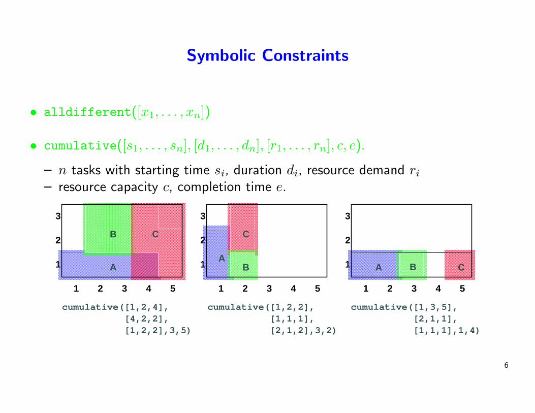
• alldifferent([x1, . . . , xn])
• cumulative([s1, . . . , sn], [d1, . . . , dn], [r1, . . . , rn], c, e).
– n tasks with starting time si, duration di, resource demand ri
– resource capacity c, completion time e.
1 2 3 4 5
1
2
3
1 2 3 4 5
1
2
3
1 2 3 4 5
1
2
3
cumulative([1,2,4], [4,2,2], [1,2,2],3,5)
cumulative([1,2,2], [1,1,1], [2,1,2],3,2)
cumulative([1,3,5], [2,1,1], [1,1,1],1,4)
A
B C
AB
C
A B C
6
Diffn Constraint
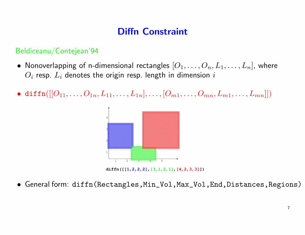
Beldiceanu/Contejean’94
• Nonoverlapping of n-dimensional rectangles [O1, . . . , On, L1, . . . , Ln], whereOi resp. Li denotes the origin resp. length in dimension i
• diffn([[O11, . . . , O1n, L11, . . . , L1n], . . . , [Om1, . . . , Omn, Lm1, . . . , Lmn]])
1 2 3 4 5
1
2
3
4
diffn([[1,2,2,2],[3,1,2,1],[4,2,3,3]])
• General form: diffn(Rectangles,Min_Vol,Max_Vol,End,Distances,Regions)
7
IP vs. CP : Algorithms
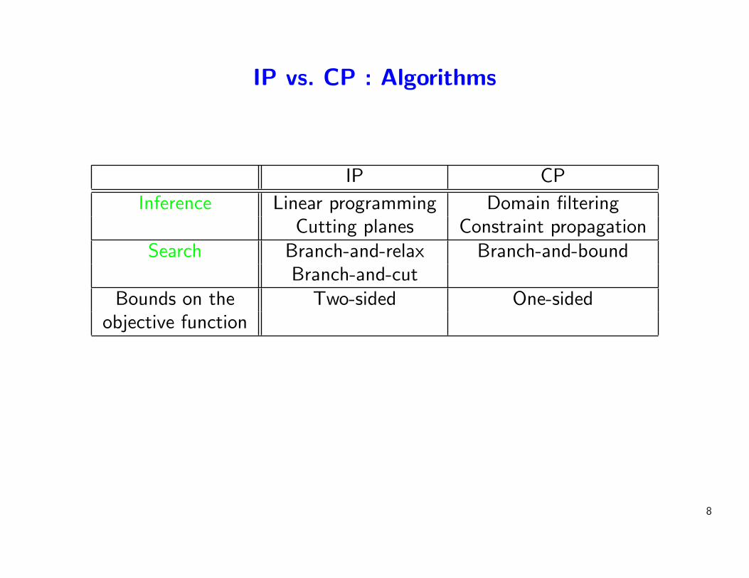
IP CP
Inference Linear programming Domain filteringCutting planes Constraint propagation
Search Branch-and-relax Branch-and-boundBranch-and-cut
Bounds on the Two-sided One-sidedobjective function
8

Local vs. Global Reasoning
Linear arithmetic constraints
3 x + y ≤ 7,3 y + x ≤ 7,
x + y = z,x, y ∈ {0, . . . , 3}
0
1
2
3
1 2 30 x
y
CP (Filtering) : x, y ≤ 2, z ≤ 4LP (Linear programming) : x, y ≤ 2, z ≤ 3.5IP (Cutting plane) : x, y ≤ 2, z ≤ 3
Global reasoning in CP ?; global constraints
9

Global Reasoning in CP
Example
• x1, x2, x3 ∈ {0, 1}
• pairwise different values
• Local consistency : 3 disequalities : x1 6= x2, x1 6= x3, x2 6= x3
; x1, x2, x3 ∈ {0, 1}, i.e. no domain reduction is possible
• Global constraint : alldifferent(x1, x2, x3); detects infeasibility (uses bipartite matching)
• Global reasoning in CP : inside global constraints
• Use domain-specific algorithms within a general solver
10

2. IP vs. CP : An Illustrating Example
11

Discrete Tomography
Bockmayr/Kasper/Zajac 98
• Binary matrix with m rows and n columns
– Horizontal projection numbers (h1, . . . , hm)– Vertical projection numbers (v1, . . . , vn)
• Properties
– Horizontal convexity (h)– Vertical convexity (v)– Connectivity (polyomino) (p)
V
H
1 232 1 1
1
3
4
2• Complexity (Woeginger’01)
– polynomial: ( ), (p,v,h)– NP-complete: (p,v), (p,h), (v,h), (v), (h), (p)
12
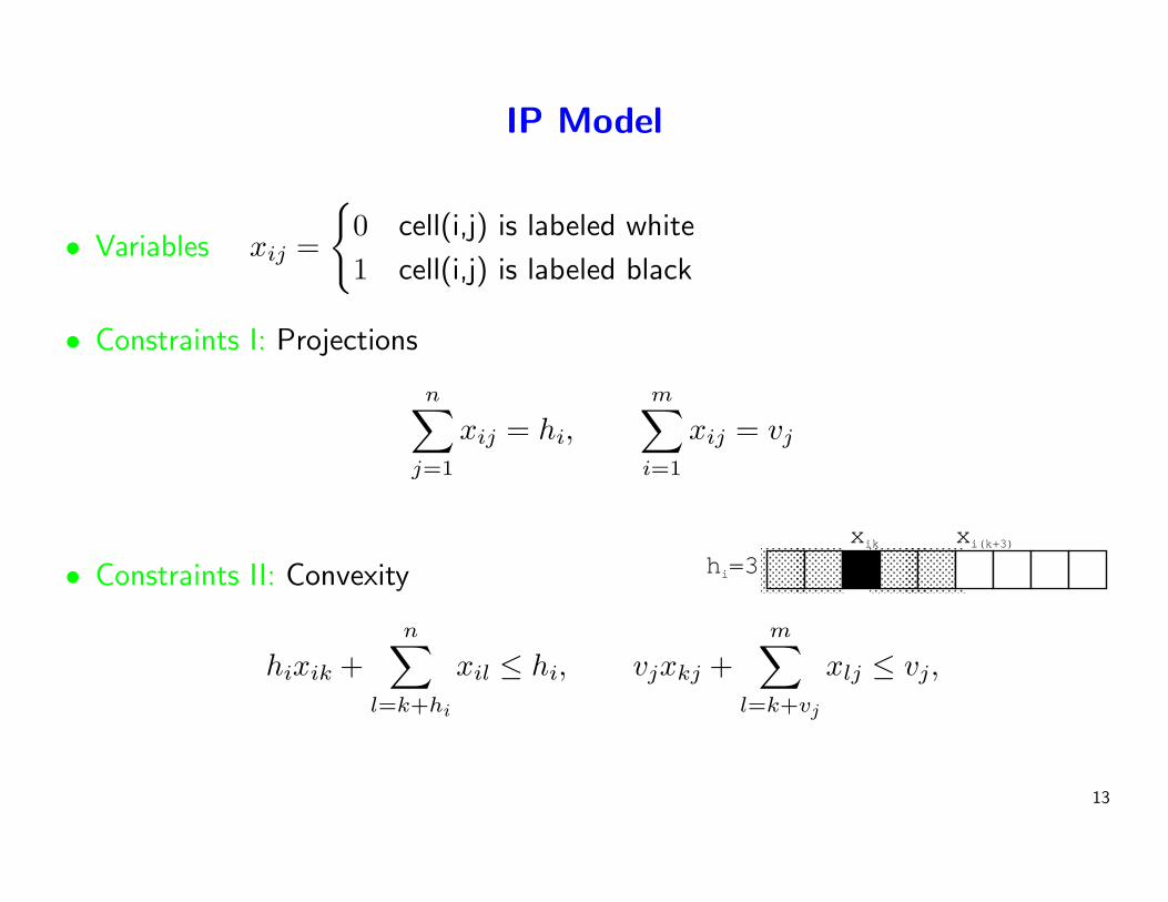
IP Model
• Variables xij =
{0 cell(i,j) is labeled white
1 cell(i,j) is labeled black
• Constraints I: Projections
n∑j=1
xij = hi,
m∑i=1
xij = vj
• Constraints II: Convexity h 3i=xik xi(k+3)
hixik +n∑
l=k+hi
xil ≤ hi, vjxkj +m∑
l=k+vj
xlj ≤ vj,
13

IP Model (contd)
• Constraints III: Connectivity
j+hi−1∑k=j
xik −j+hi−1∑
k=j
x(i+1)k ≤ hi − 1
h 4i=
xi2
3=hi+1
• Various linear arithmetic models possible, e.g. convexity
• Enormous differences in size and running time, e.g. 1 day vs. < 1 sec
• Large number of constraints (∼ 3mn in the above model)
14

Finite Domain Model
• Variables
– xi start of the horizontal convex block in row i, for 1 ≤ i ≤ m– yj start of the vertical convex block in column j, for 1 ≤ j ≤ n
Y
VH 1 353 1 1
2
3
5
2
2
2 31 1 3 3
2
1
2
3
3
X
• Domain
– xi ∈ [1, . . . , n− hi + 1], for 1 ≤ i ≤ m– yj ∈ [1, . . . ,m− vj + 1], for 1 ≤ j ≤ n
15

Conditional Propagation
• Projection/Convexity modelled by FD variables
• Compatibility of xi and yj
xi ≤ j < xi + hi ⇐⇒ yj ≤ i < yj + vj
for 1 ≤ i ≤ m and 1 ≤ j ≤ n
row i
• Conditional propagation
if xi ≤ j then (if j < xi + hi then (yj ≤ i, i < yj + vj))
16
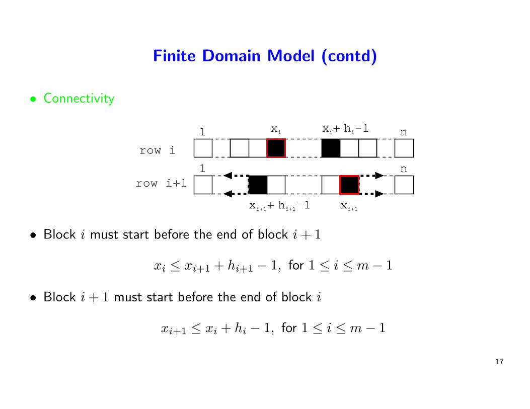
Finite Domain Model (contd)
• Connectivity
xi hi
hi+1xi+1+ -1
xi+ -1
xi+1
row i
row i+1
1 n
1 n
• Block i must start before the end of block i + 1
xi ≤ xi+1 + hi+1 − 1, for 1 ≤ i ≤ m− 1
• Block i + 1 must start before the end of block i
xi+1 ≤ xi + hi − 1, for 1 ≤ i ≤ m− 1
17

Cumulative
-
63 4 3 7 6 4 4 3 4 2
1277445541
3 4 3 7 6 4 4 3 4 2
18

2d and 3d Diffn Model
1277445541
3 4 3 7 6 4 4 3 4 2
���
���
���
���
���
���
���
���
���
���
���
���
1277445541
3 4 3 7 6 4 4 3 4 2
����
��
��
��
��
���
������
���
������
������
������
���
���
���
���
���
���
19

3. Combining IP and CP
20

Generic MIP/CP Model
Bockmayr/Pisaruk’03
max cx + dz, (1)
Ax + Gz ≤ b, (2)
Fi(xi) = 0, i = 1, . . . ,m, (3)
l ≤ x ≤ u, x ∈ Zn, l′ ≤ z ≤ u′, z ∈ Rp, (4)
where
• xi = (xi1, . . . , xik(i)) consists of some components of x = (x1, . . . , xn), and
• Fi : Zk(i) → {0, 1} is monotone, i.e., x ≤ y ⇒ F (x) ≤ F (y).
21

Monotone constraints
• Let x, y ∈ [l, u] with F (x) = 0 and F (y) = 1.
• For F : [l, u] → {0, 1} monotone, we cannot have y ≤ x. Therefore
(x1 ≤ y1 − 1) ∨ (x2 ≤ y2 − 1) ∨ . . . ∨ (xn ≤ yn − 1) (5)
• If yi = li ∨ yi = ui, for i = 1, . . . , n, then (5) is equivalent to∑i:yi>li
xi ≤ (∑
i:yi>li
yi )− 1 (6)
• In general, inequality (6) is stronger than the disjunction (5).
22

Binary Case
• If [l, u] = {0, 1}n, then (6) and (5) are equivalent.
• (6) can be rewritten as the cardinality inequality∑i∈S(y)
xi ≤ |S(y)| − 1, (7)
where S(y) = {j : yj 6= 0} denotes the support of the vector y.
• It follows
F−1(0) = {x ∈ {0, 1}n : F (x) = 0} (8)
= {x ∈ {0, 1}n :∑
i∈S(y)
xi ≤ |S(y)| − 1, y ∈ F−1(1)}, (9)
23

Heuristic Separation
• Separate x ∈ [0, 1]n from conv(F−1(0))
1. Sort components of x in nondecreasing order: xπ(1) ≥ . . . ≥ xπ(n).
2. Let r ∈ {1, . . . , n} be the largest index such that∑r
j=1 xiπ(j) > r − 1.
3. Obtain a 0-1 vector y ∈ {0, 1}n by yπ(j) ={
1, if 1 ≤ j ≤ r,0, if r + 1 ≤ j ≤ n
.
4. If F (y) = 1, the inequality∑r
j=1 xπ(j) ≤ r−1 separates x from conv(F−1(0)).
• The procedure may fail to separate x from conv(F−1(0)) even if x 6∈conv(F−1(0)).
• However, it always separates infeasible integral points.
24
IP/CP Branch and Cut
• Start with the IP program (1), (2), and (4).
• Assume x has to be tested for feasibility (when solving some LP subproblem).
• For i = 1, . . . ,m, use the heuristic together with CP algorithms to separate xi
from conv(F−1i (0)).
• Since the heuristic always separates infeasible integer points, the output is anoptimal feasible solution to problem (1)–(4) (if it exists).
25

Multiple Machine Scheduling Problem
Jain/Grossmann’01
• n tasks, m dissimilar machines.
• any task can be processed on any machine.
• processing cost cij and processing time pij for task i on machine j
• ri release date, di due date of task i.
• carry out all the tasks at the least possible cost.
Main decisions
1. Assignment of tasks to machines.
2. Sequencing of tasks on each machine, and starting time for each task.
26

Combined IP/CP Model
• xij = 1 if task i is assigned to machine j, xij = 0 otherwise.
• Fj(xj) = 0 if the tasks in S(xj) can be done on machine j respecting releaseand due dates.
min∑n
i=1
∑mj=1 cijxij∑m
j=1 xij = 1, i = 1, . . . , n,∑mj=1 pijxij ≤ di − ri, i = 1, . . . , n,∑ni=1 pijxij ≤ max1≤i≤n di −min1≤i≤n ri, j = 1, . . . ,m,
Fj(x1j, . . . , xnj) = 0, j = 1, . . . ,m,
xij ∈ {0, 1}, i = 1, . . . , n; j = 1, . . . ,m.
27

Testing Feasibility by CP
• Handle Fj(xj) = 0 by solving a CP program with a single global constraint.
• Let Dj(xj) = maxi∈S(xj) di, and assume S(xj) = {s1, . . . , sk}, k = |S(xj)|.
• Then Fj(xj) = 0 iff the CP problem
tsi∈ [rsi
, dsi− psi,j], i = 1, . . . , k,
cumulative([[ts1, ps1,j, 1], . . . , [tsk, psk,j, 1]], 1, Dj(xj))
has a solution.
• Computational results: Bockmayr/Pisaruk’03
• Further applications: Supply chain optimization (LISCOS)
28

Conclusion
• IP and CP
• Model building: Language
• Model solving: Algorithms
• Case study: Discrete tomography
• Combining IP and CP: Cut generation for IP using CP
29

References
• A. Bockmayr and J. N. Hooker: Constraint programming. In Handbooks inOperations Research and Management Science. Vol. 12: Discrete Optimization(Eds. K. Aardal, G. Nemhauser, and R. Weismantel), Chapter 10, 559 - 600,Elsevier, 2005.
• A. Bockmayr and N. Pisaruk: Detecting Infeasibility and Generating Cuts for MIPusing CP. 5th International Workshop on Integration of AI and OR Techniques inConstraint Programming for Combinatorial Optimization Problems, CPAIOR’03,Montreal, 2003. Revised version to appear in Computers & Operations Research
30