1

An Optimal and Distributed Method for VoltageRegulation in Power Distribution Systems

Baosen Zhang, Member, IEEE, Albert Y.S. Lam, Member, IEEE,Alejandro Domınguez-Garcıa, Member, IEEE, and David Tse, Fellow, IEEE.

Abstract—This paper addresses the problem of voltage regu-lation in power distribution networks with deep-penetration ofdistributed energy resources, e.g., renewable-based generation,and storage-capable loads such as plug-in hybrid electric vehicles.We cast the problem as an optimization program, where theobjective is to minimize the losses in the network subject toconstraints on bus voltage magnitudes, limits on active and reac-tive power injections, transmission line thermal limits and losses.We provide sufficient conditions under which the optimizationproblem can be solved via its convex relaxation. Using datafrom existing networks, we show that these sufficient conditionsare expected to be satisfied by most networks. We also providean efficient distributed algorithm to solve the problem. Thealgorithm adheres to a communication topology described by agraph that is the same as the graph that describes the electricalnetwork topology. We illustrate the operation of the algorithm,including its robustness against communication link failures,through several case studies involving 5-, 34- and 123-bus powerdistribution systems.

I. INTRODUCTION

Electric power distribution systems will undergo radicaltransformations in structure and functionality due to the adventof initiatives like the US DOE Smart Grid [1], and itsEuropean counterpart Electricity Networks of the Future [2].These transformations are enabled by the integration of (i)advanced communication and control, (ii) renewable-basedvariable generation resources, e.g., photovoltaics (PVs), and(iii) new storage-capable loads, e.g., plug-in hybrid electricvehicles (PHEVs). These distributed generation and storageresources are commonly referred to as distributed energyresources (DERs). It has been acknowledged (see, e.g., [3])that massive penetration of DERs in distribution networks islikely to cause voltage regulation problems due to the factthat typical values of transmission line resistance-to-reactance,r/x, ratios are such that bus voltage magnitudes are fairlysensitive to variations in active power injections (see, e.g., [4]).Similarly massive penetration of PHEVs can potentially createsubstantial voltage drops [5]. The objective of this paper isto address the problem of voltage regulation in electric powerdistribution networks with deep penetration of DERs.

B. Zhang is with the Department of Civil and Environmental Engi-neering and the Department of Management and Science Engineering atStanford University; E-mail: zhangbao@stanford.edu. A.Y.S. Lam is withthe Department of Computer Science at Hong Kong Baptist University; E-mail: albertlam@ieee.org. A. Domınguez-Garcıa is with the Department ofElectrical and Computer Engineering of the University of Illinois at Urbana-Champaign; E-mail: aledan@illinois.edu. D. Tse is with the Department ofElectrical Engineering at Stanford University; E-mail: dntse@stanford.edu

As of today, voltage regulation in distribution networksis accomplished through tap-changing under-load transform-ers, set voltage regulators, and fixed/switched capacitors.While these devices—the operation of which is mechanical innature—are effective in managing slow variations (on the time-scale of hours) in voltage, their lifetime could be dramaticallyreduced from the increased number of operations needed tohandle faster voltage variations due to sudden changes (on thetime-scale of minutes) in active power generated or consumedby DERs. An alternative to the use of these voltage regulationdevices for handling fast variations is to utilize the powerelectronics interfaces of the DERs themselves.

While active power control is the primary function of theseinterfaces, when being properly controlled, they can alsoprovide reactive power. Thus, they provide a mechanism tocontrol reactive power injections, which in turn can be usedfor voltage control (see, e.g., [6], [7]). In this regard, thereare existing PV rooftop and pole-mount solutions that providesuch functionality (see, e.g., [8], [9]). These solutions areendowed with wireless [8], and power-line communications[9], which is a key for controlling a large number of de-vices without overlaying a separate communication network.Additionally, as noted earlier, bus voltages in a distributionnetwork are sensitive to changes in active power injections.Thus, storage-capable DERs, and demand response resources(DRRs), provide a second voltage control mechanism as theycan be used, to some extent, to shape active power injections.

This paper proposes a method for voltage regulation indistribution networks that relies on the utilization of reactive-power-capable DERs, and to some extent, on the control ofactive power injections enabled by storage-capable DERs andDRRs. This method is intended to supplement the action ofconventional voltage regulation devices, while i) minimizingtheir usage by handling faster voltage variations due to changesin renewable-based power injections, and ii) having them in-tervene only during extreme circumstances rather than minor,possibly temporary, violations. In this regard, in subsequentdevelopments, we assume that there is a separation in the(slow) time-scale in which the settings of conventional voltageregulation devices are adjusted and the (fast) time-scale inwhich our proposed method operates. For instance, the set-tings of conventional devices can be optimized every hour inanticipation of the overall change in load (e.g., air conditionersbeing turned on in a hot afternoon). Then, within each hour,our method is utilized to regulate voltage in response to fastvariations in DER-based power injections. A more detaileddescription of the ideas above is provided in Section II-B.

2

The voltage regulation problem can be cast as a optimizationprogram where the objective is to minimize network losses1

subject to (i) constraints on bus voltage magnitudes, (ii) upperand lower limits on active and reactive power injections, (iii)upper limits on transmission line flows, and (iv) upper limitson transmission line losses. The decision variables are the busvoltages; however the actual control mechanism to fix theseare reactive (and to some extent active) power injections inthe bus of the network.

The contributions of this paper are two fold. First, we es-tablish sufficient conditions under which the voltage regulationproblem can be solved via an equivalent semidefinite program-ming (SDP) problem, thus convexifying the original problem.This equivalence also leads to a simple method to establishwhether or not the original problem has a feasible solutionbased on the solution of the convexified problem. However, itis important to note that even if the convexified SDP providesthe solution to the original optimization problem, existingalgorithms for solving SDPs are not computationally efficientfor solving large problems [10]. Therefore, these algorithmsare not practical for realizing our ideas in a realistic powerdistribution network with thousands of buses. Furthermore,even if there is a centralized solver with sufficient computingpower, the communication infrastructure may not be able toreliably transmit all problem data to a centralized location withsmall enough delays. This is where the second contribution ofour work lies—the development of a distributed algorithm forefficiently solving convexified SDPs on tree networks; as itwill shown later, a key feature of this algorithm is that isrobust against communication failures.

Previous works that addressed the voltage regulation prob-lem in distribution networks also cast it as an optimizationproblem; however, in contrast with our work, the solutionmethods proposed in these earlier works are sub-optimal, andin most cases, they rely on a centralized decision maker thathas access to all the data defining the problem [11], [12].For example in [13], the authors propose the use of reactive-power-capable DERs for voltage control and the objective isto minimize the DER reactive power contributions subject tothe power flow equations and other constraints. However, thesolution approach proposed in [13] relies on linearizing thepower flow equations around some operating point, rendering alinear program; therefore, this approach provides a sub-optimalsolution. In the same vein, and although the objective functionis different to the one considered in [13], the solution proposedin [14] also relies on linearization.

Other optimization-based approaches to address the voltageregulation problem in distribution networks rely on optimalpower flow (OPF) solvers developed for transmission networks(see, e.g., [15], [16]). For instance, in [16], the authors usea Newton-type method to solve the Lagrange dual of theoptimization program they consider in their problem; however,since the primal problem is, in general, not convex, there isno guarantee that the solution of the dual problem is globallyoptimal, or even physically meaningful.

1Any objective function that is strictly increasing can be used and all ofthe results in this paper remains unchanged. We focus on loss minimizationdue to its relevance for long-run economic savings.

The key to solve the the voltage regulation problem isto wite it as a rank-constrained SDP [17], where the de-cision variable is a positive semidefinite matrix constrainedto have rank 1, which, in general, makes the problem notconvex. The problem can be convexified by dropping the rank-1 constraint—the conundrum is then to establish when thesolution of the convexified problem also provides a globalsolution to the original non-convex problem.

Recently there has been a sequence of papers on attemptingto answer the question above spurred by the observation in[18] that the convex relaxation observed above is tight formany IEEE benchmark transmission networks. Several inde-pendent works [19]–[21] provided a partial answer: the convexrelaxation is tight if the network has a tree topology andcertain constraints on the bus power injections are satisfied. Allthese results, which are particularly relevant for distributionnetworks, were unified and strengthened in [22] through ainvestigation of the underlying geometry of the optimizationproblem. It is important to note that, even in the situationswhere the convex relaxation is tight, there might be multiplelocal optimal solutions and local search algorithms may notconverge to the globally optimal one (see [20] for a furtherdiscussion on this). Finally, it is well known (see, e..g, [23])that solution methods to OPF-type problems for transmissionnetworks tend to perform poorly in distribution networks dueto the r/x values.

An independent—but related—work has recently appearedin [24]. Although, a direct comparison of both works isdifficult due to the difference in assumptions and constraints(for example [24] does not require all buses to have DERs),the solution method proposed by the authors in [24] is alsoglobally optimal; however, their solution method requires acentralized processor, whereas as it is shown later, our solutionmethod is amenable for a distributed implementation. Withrespect to this, recent independent works to ours are the ones in[25] and [26]; where the authors in [25] propose a distributedalgorithm to solve convex relaxations for OPF-type problemsin general networks and the authors in [26] considered demandresponse in the distribution network.

This paper builds on the results of [19], [22] and extendsthem by taking into account the reactive power injections,and considering tight voltage magnitude constraints. Previousresults either: (i) ignore reactive power (e.g. [22], [27]–[29] ),(ii) assume there are not active lower bounds (e.g. [18], [26]),or (iii) assume that there are no voltage upper bounds (e.g[28]).

The remainder of this paper is organized as follows. Sec-tion II discusses the voltage regulation problem and formulatesits solution as an optimization problem. Section III statesthe main theoretical result of the paper, while Section IVprovides a sketch of the proof (the complete proof is providedin Appendix). Section V proposes a distributed algorithm tosolve the optimization problem, the performance of which isillustrated in Section VI via case studies. Concluding remarksare presented in Section VII.

3

II. PRELIMINARIES AND PROBLEM FORMULATION

This section introduces the model for the class of powerdistribution systems considered in this work; in the process,relevant notations used throughout the paper are also in-troduced. Subsequently, we discuss the problem of voltageregulation in distribution networks with deep DER penetration.Additionally, we articulate a potential solution that coordinates(a) the utilization of conventional voltage regulation devicesfor handling slower voltage variations, and (b) the use of DERsand DRRs for handling faster variations. The section concludeswith the formulation of an optimization problem that enablesthe realization of (b) above.

A. Power System Distribution Model

Consider a power distribution network with n buses. As oftoday, such networks are mostly radial with a single sourceof power injection referred to as the feeder (see, e.g., [30]).Thus, the network topology can be described by a connectedtree, the edge set of which is denoted by E , where (i, k) ∈ Eif i is connected to k by a transmission line; we write i ∼k if bus i is connected to bus k and i 6∼ k otherwise, and(i, k) to denote a transmission line connected between buses iand k. Typical examples of power distribution networks withsuch tree topologies are the IEEE 34- and 123-bus distributionsystems; the topologies of these systems, which are used inthe case studies of Section VI, are displayed in Figs. 7 and 8respectively.

Let Vi = |Vi|∠θi denote bus i voltage, and define thecorresponding bus voltage vector v = [V1 V2 · · · Vn]T ∈Cn. Similarly, let Pi and Qi denote, the active and reac-tive power injections in bus i respectively, and define thecorresponding active and reactive power injection vectorsp = [P1 P2 · · · Pn]T , q = [Q1 Q2 · · · Qn]T . Letyik = gik − jbik, with bik > gik > 0, denote the admittance2

of line (i, k), and let yii = jbii denote bus i shunt admittance.Then, the power flow equations can be compactly written as

p + jq = Re{diag(vvHYH)}+ jIm{diag(vvHYH)}, (1)

where Y = [Yik] is the bus admittance matrix ( we use A[i, k]to denote the (i, k)th entry of a matrix A), vH (YH ) denotesthe Hermitian transpose of v (Y), and diag(·) returns thediagonal of a square matrix as a column vector. The activepower flow through each transmission line (i, k) is given by

Pik = |Vi|2gik + |Vi||Vk|[bik sin(θik)− gik cos(θik)], (2)

whereas the reactive power flow through each transmissionline (i, k) is given by

Qik = |Vi|2bik − |Vi||Vk|[gik sin(θik) + bik cos(θik)], (3)

where θik := θi − θk.

2We adopt the standard assumption that, in normal operating conditions,lines are inductive and the inductive effects dominate resistive effects (see,e.g., [31]. Additionally, although the convention is to write yik = gik+jbik ,we chose to flip the sign of the imaginary part as it simplifies subsequentdevelopments.

t0 t1 t2

Instants at which conventional voltageregulation devices are set

time

Instants at which DER/DRRreferences are set

Fig. 1. Time-scale separation between the instants in which the settings ofconventional voltage regulation devices are decided, and the instants in whichthe reference of DER and DRRs are set.

B. Voltage Control in Networks with Deep DER Penetration

The objective of the paper is to address the problem ofvoltage regulation in power distribution networks with deeppenetration of DERs; specifically, the focus is on the problemof mitigating voltage variability across the network due toto fast (and uncontrolled) changes in the active generated orconsumed by DERs. To this end, we rely on i) the use of thepower electronics interfaces of the DERs to locally providesome limited amount of reactive power; and ii) to some extent,on the use of storage-capable DERs and DRRs to locallyprovide (or consume) some amount of active power. In otherwords, we have a limited ability to shape the active/reactivepower injection profile. With respect to this, it is importantto note that this ability to shape the active/reactive powerinjection profile, which in turn will allow us to regulate voltageacross the network, and it is intended to supplement theaction of conventional voltage regulation devices (e.g., tap-changing under-load transformers, set voltage regulators, andfixed/switched capacitors).

In practice, in order to realize the ideas above, we envisiona hierarchical control architecture; there is a separation in the(slow) time-scale in which the settings of conventional voltageregulation devices are adjusted via the solution to some opti-mization problem, and the (fast) time-scale in which voltageregulation through active/reactive power injection shaping isaccomplished. Then, given that fast (and uncontrolled) changesin the DERs active generation (consumption) might causethe voltage to deviate from this reference voltage, a secondoptimization is performed at regular intervals (e.g., everyminute). The timeframe in which the settings of conventionaldevices are decided and the reference setting of DERs/DRRs isgraphically depicted in Fig. 1. The solution of this minute-by-minute optimization will provide the amount of active/reactivepower that needs to be locally produced or consumed so asto track the voltage reference. In order words, the minute-by-minute optimization provides the reference values for theamount of active/reactive power to be collectively provided (orconsumed) on each bus of the network within the next minuteby reactive-power-capable and/or storage-capable DERs andDRRs. These reference values are then passed to the DERsand DRRs local controllers, which will adjust their outputaccordingly—note that the time-scale in which DER/DRR lo-cal controllers act (on the order of milliseconds (see, e.g., [32],[33]), is much faster than the minute-to-minute optimization.Here, it is important to note that the DERs and DRRs are

4

only attempting to correct voltage deviation from the nominalvalue due to variations in power injections around the powerinjection profile used to set the conventional voltage regulationdevices.

C. Voltage Regulation via DERs/DRRs: Problem FormulationAs stated earlier, the focus of this paper is on developing

mechanisms to mitigate voltage variability across the networkdue to fast (and uncontrolled) changes in the active generatedor consumed by DERs; thus, subsequent developments onlydeal with the inter-hour minute-by-minute optimization men-tioned above. As argued in Section II-B, we assume that at thebeginning of each hour, the settings of conventional voltageregulation devices are optimized, which in turns prescribe thevalues that each individual bus voltage can take to some volt-age reference V refi . In order to achieve the voltage regulationgoal above, we rely on a limited ability to locally produceand/or consume some limited amount of active/reactive power,and cast the voltage regulation problem as an optimizationprogram with the objective of minimizing network losses.

Let Lik(Vi, Vk) = Pik+Pki. The total losses in the networkare given by L(v) :=

∑i,k:(i,k)∈E Lik(Vi, Vk), and the voltage

regulation problem can be formulated as

minv

L(v) (4a)

s.t. |Vi| = V refi ,∀i (4b)

P i ≤ Pi ≤ P i,∀i (4c)

Qi≤ Qi ≤ Qi,∀i (4d)

|Pik| ≤ P ik, ∀i ∼ k (4e)

Lik(Vi, Vk) ≤ Lik, ∀i ∼ k (4f)

Pi =∑k∼i

Pik (4g)

Qi =∑k∼i

Qik. (4h)

The constraints in (4b) capture the voltage regulation goal.The constraints in (4c) and (4d) describe the limited abilityto control active/reactive power injections on each bus i;P i (P i) and Qi (Q

i), denote the upper (lower) limits on

the amount of active and reactive power that each bus ican provide, respectively. The constraints in (4e) capture linepower flow limits, while (4f) imposes loss limits on individuallines. Without loss of generality and to ease the notations insubsequent development, hereafter we assume V refi = 1 p.u.for all i. Note that active power and reactive power need notbe controllable at every bus. If for a particular bus they are notcontrollable, in the optimization problem we set the bus activeand/or reactive power upper and lower bounds to be equal,which essentially fixes the active and/or reactive on that bus.

The optimization problem in (4) is difficult for two reasons:i) it is not convex due to the quadratic relationship betweenbus voltages and powers; and ii) depending on the size of thenetwork, there could potentially be a large number of variablesand constraints. Section III and Section IV address i) byconvexifying the problem in (4), while Section V addresses ii)by proposing a computationally efficient distributed algorithmto solve the resulting convexified problem.

III. CONVEX RELAXATION

In this section, we state the main theoretical result, whichis that under certain conditions on the angle differencesbetween adjacent buses and the lower bounds on reactivepower injections, the nonconvex problem in (4) can be solvedexactly by solving its convex SDP relaxation. We note thatSDP relaxation is not the only possible convex relaxation, e.g.,[24] proposes a SOCP relaxation. In order to state the SDPrelaxation, it is convenient to rewrite the problem in (4) inmatrix form.

A. Voltage Regulation Problem Formulation in Matrix From

Let Ei ∈ Rn×n, with Eii = 1 and all other entriesequal to zero, and define Ai = 1

2 (YHEi + EiY), andBi = 1

2j (YHEi − EiY). Then, the active and reactivepower injections in bus i are given by Pi = Tr(Aivv

H),and Qi = Tr(Bivv

H), respectively, where Tr(·) is the traceoperator. For each (i, k) ∈ E , define a matrix Aik, with its(l,m)th entry given by

Aik[l,m] =

Re{Yik} if l = m = i−Yik/2 if l = i and m = k−Y Hik /2 if l = k and m = i0 otherwise;

(5)

the active power flow through the (i, k) line is given by Pik =Tr(Aikvv

H). Let Gik = Aik + Aki. Then, we can rewrite(4) as

minv

n∑i=1

Tr(AivvH) (6a)

s.t. |Vi| = 1,∀i (6b)

P i ≤ Tr(AivvH) ≤ P i,∀i (6c)

Qi≤ Tr(Bivv

H) ≤ Qi,∀i (6d)

Tr(GikvvH) ≤ Lik,∀i ∼ k (6e)

|Tr(AikvvH)| ≤ P ik,∀i ∼ k. (6f)

Note that the outer product vvH is a positive semidefiniterank-1 n×n matrix. Conversely, given a positive semidefiniterank-1 n × n matrix, it is always possible to write it as anouter product of a vector and itself. Thus, we can rewrite (6)as

minW<0

n∑i=1

Tr(AiW) (7a)

s.t. W[i, i] = 1,∀i (7b)

P i ≤ Tr(AiW) ≤ P i,∀i (7c)

Qi≤ Tr(BiW) ≤ Qi,∀i (7d)

Tr(GikW) ≤ Lik,∀i ∼ k (7e)

|Tr(AikW)| ≤ P ik,∀i ∼ k (7f)rank(W) = 1, (7g)

where the rank-1 constraint in (7g) makes the problem notconvex.

5

B. Convexification

The problem in (7) is not convex due to the rank-1 constraint(7g); by removing it, we obtain a relaxation that is convex:

minW<0

n∑i=1

Tr(AiW) (8a)

s.t. W[i, i] = 1,∀i (8b)

P i ≤ Tr(AiW) ≤ P i,∀i (8c)

Qi≤ Tr(BiW) ≤ Qi,∀i (8d)

Tr(GikW) ≤ Lik,∀i ∼ k (8e)

|Tr(AikW)| ≤ P ik,∀i ∼ k; (8f)

This convex relaxation is not always tight since the rank of thesolution to (8) could be greater than 1. Thus the solution to (8)does not always coincide with the solution to (7). However, byimposing two conditions that are widely held in practice, thenon-convex problem in (7) can be solved exactly by solving(8), as stated in the following theorem.

Theorem 1. Consider a power distribution network with a treetopology. Define θPik to be the smallest positive solution to theequation P ik = Pik, with Pik given in (2) for |Vi| = |Vk| = 1;and θLik = cos−1(1 − Lik

2gik) if Lik

2gik≤ 2 and θLik = ∞ if

Lik

2gik> 2. Let θik = min(θPik, θ

Lik). Suppose θik satisfies

− tan−1 (bik/gik) < θik < tan−1 (bik/gik) ; (9)

and reactive power injection lower bounds satisfy

Qi< βi, i = 2, . . . , n, (10)

with βi =∑k:k∈C(i) bik − gik sin(θik) − bik cos(θik),

where C(i) is the set of all neighbors of i and θik =min(tan−1( gikbik ), θik). Let W∗ be an optimal solution to therelaxed problem in (8). Then

1) If W∗ is rank 1, then W∗ = v∗(v∗)H for somevector v∗. Furthermore, v∗ is the optimal solution tothe voltage regulation problem stated in (4).

2) If rank(W∗) > 1, then there is no feasible solution tothe voltage regulation problem stated in (4).

3) If (8) is infeasible, then the the voltage regulationproblem stated in (4) is infeasible.

The theorem is proved for a two-bus network in Section IVby studying the geometry of the feasibility set of the originalproblem in (6) and that of its convex relaxation in (8). Theintuition and geometric insight developed by studying the two-bus network carries over to a general tree network and the fullproof is provided in the Appendix.

IV. SKETCH OF THEOREM 1 PROOF

The insights into Theorem 1 are obtained by studying thegeometry of the sets that result from the constraints on linepower flows and power injections as described in (4c)–(4f).This geometric view was explored in previous works [19],[22]. Here, we revisit the results of [22] and generalize themto include limits on reactive power injections.

Fig. 2. The active line flow region Fik , the reactive flow region Gik , andthe linear transformation Hik between them.

Fig. 3. The flow region under thermal loss constraints (left) and line flowconstraints (right). The bold curves indicate the feasible part.

A. Active and reactive line flow regions

First, recall from (7b) that |Vi| = |Vk| = 1 p.u. Then, letFik ∈ R2 and Gik ∈ R2 denote the regions that contain allthe [Pik, Pki]

T and [Qik, Qki]T that can be achieved from (2)

and (3) by varying θik between 0 and 2π; it is easy to seethat for 0 < θik < 2π, (2) and (3) are linear transformationsof a circle. Thus, as depicted in Fig. 2, the active and reactiveline flow regions Fik and Gik are ellipses. The center of Fik(Gik) is [gik, gik]T ([bik, bik]T ). Its major axis is parallel to[1,−1]T ([1, 1]T ) and has length bik (bik), while its minoraxis is parallel to [1, 1]T ([1,−1]T ) and has length gik (gik).Both ellipses are related by a linear invertible mapping: Gik =HikFik, with

Hik =1

2bikgik

[b2ik − g2ik b2ik + g2ikb2ik + g2ik b2ik − gik

]. (11)

The line flow constraints in (4e) and the thermal lossconstraints in (4f) appear as linear constraints on the line flowregions as shown in Fig. 3. Thus, for each line (i, k), wecan replace both constraints by a single one, which has theform of the line flow constraint for properly defined upperlimits. We adopt this convention in subsequent developments.Furthermore, since the ellipses have empty interior, this flowconstraint can be translated into angle constraints on θik ofthe form |θik| ≤ θik. Conversely, an angle constraint on θikcan be converted into a flow constraint. Let Fθ,ik and Gθ,ikdenote, respectively, line (i, k) angle-constrained active andreactive line flow regions, then

Fθ,ik = {[Pik, Pki]T : Pik = gik[1− cos(θik] + bik sin(θik),

Pki = gik[1− cos(θik]− bik sin(θik), |θik| ≤ θik},Gθ,ik = {[Qik, Qki]T : Qik = bik[1− cos(θik]− gik sin(θik),

Qki = bik[1− cos(θik] + bik sin(θik), |θik| ≤ θik}.

6

Fig. 4. Angle-constrained active line flow region and its convex hull (filledin blue region) when relaxation is tight (left) and when relaxation does notprovide solution to the original problem (right).

Fig. 5. Active power injection region (left) and reactive power injectionregion (right) under reactive power injection lower bound.

B. Feasible Region of a Two-Bus Network

Consider a system with only two buses connected by a line(1, 2), with P1 (Q1) and P2 (Q2) denoting the active (reactive)power injections on bus 1 and 2, respectively; for a two-bussystem, P1 = P12 (Q1 = Q12) and P2 = P21 (Q2 = Q21).The relaxed problem in (8) convexifies the feasible region ofthe problem (7) by filling up the corresponding ellipses asshown in Fig. 4. Note that since the objective is to minimizethe total power loss (i.e. P1 +P2), the solution to the relaxedproblem will be in the lower left part of the relaxed feasibleregion. The relaxation is tight if the relaxed solution lies on theboundary of the ellipse, so that a rank-1 solution is recovered.

The condition in (9) is a constraint on the maximum angledifference across the line. Intuitively, this angle constraint issuch that only the lower left part of the line flow ellipses isfeasible. For example, this condition is satisfied by the angle-constrained regions in Fig. 4; this figure shows the intersectionof bus power constraints with the angle-constrained activeinjection regions. In Fig. 4(a), both bus power constraints areupper bounds. Since the optimal solution of the power lossproblem occurs in the lower left corner, the convex relaxationis tight; this is an example of case 1 in Theorem 1. InFig. 4(b), both bus power constraints are lower bounds; in thiscase the optimal solution is inside the ellipses and thereforerankW∗ = 2. On the other hand, the original problem isinfeasible; this is an example of case 2 in Theorem 1.

It is important to note that the observations made in Fig. 4hold as long as the angle-constrained injection region onlyincludes the lower left half of the ellipse (as described by (9)).From thermal data for some common lines in [30], we expectthat the angle to be constrained to θik ∈ [−10◦, 10◦]. Even fora relatively small bik/gik ratio of 2, θik = tan−1(bik/gik) =63.4◦ and the condition |θik| < θik is always satisfied.Therefore in most practical networks, it is expected that thethermal constraints in the network are small enough that thecondition in (9) should be satisfied almost always.

The second condition in (10) is to ensure that the reactivelower bound is large enough such that Qi > Q

ifor all feasible

Qi. If the reactive lower bounds are tight at the optimalsolution of the relaxed problem, then the rank of the optimalmatrix W∗ is not necessarily 1. Figure 5 shows the reasonthat the condition on the reactive power lower bounds areneeded. Figure 5(b) gives the reactive injection region witha tight reactive lower bound on bus 2. Figure 5(a) shows thecorresponding active power injection region. Observe that itis possible for the optimal solution of the relaxed problem tobe of rank 2, while the original problem remains feasible. Thecondition Q

i< βi rules out this phenomenon by ensuring that

the reactive power lower bounds are never tight.

C. General Tree Networks

The geometrical intuition developed for the two-bus networkcarries over to a general tree network due to the fact thatflows on each line are independent (no cycles), and activeand reactive power injections can be described, respectively,as linear combinations of active and reactive line flows. Theseare the main ideas used in proving Theorem 1; the interestedreader is referred to the Appendix for the full proof.

V. A DISTRIBUTED ALGORITHM FOR SOLVING THECONVEXIFIED PROBLEM

In Section III, we showed that the SDP program in (8)is a convex relaxation of the voltage regulation problem in(4). Since the objective is to regulate the voltages in thepresence of fast-changing power injection that, e.g., arise fromrenewable-based generation; the optimization problem needsto be solved no slower than the time-scale at which theseinjections significantly change. General-purpose SDP solversscale poorly as the problem size increases [10]. Thus for largedistribution networks with hundreds or thousands of buses,solving the SDP problem in a minute to sub-minute scale ischallenging. Furthermore standard solvers for SDP problemsare centralized; i.e., it is assumed that all the data definingthe problem is available to a single processor. However thecommunication infrastructure in a distribution network maynot be able to transmit all the data to a centralized locationfast enough. By exploiting the tree structure of distributionnetworks, we propose a distributed algorithm to solve (8) thatonly requires communication between neighboring buses. Thiscommunication requirement is reasonable since that neigh-boring buses are typically physically closest to each other aswell. Therefore any wireless communication technology (andobviously power line communication) would enable nearestneighbors to communicate to each other.

A. Algorithm Derivation

The proposed algorithm consists of two stages: local op-timization and consensus. In the local optimization stage,each node solves its own local version of the problem. Inthe consensus stage, neighboring nodes exchange Lagarangianmultipliers obtained from the solutions to their correspondinglocal optimums, with the goal of equalizing the phase angledifferences across a line from both of its ends.

7

Let Ni be the set of buses directly connected to bus i bytransmission lines, together with bus i itself, i.e., Ni = {k :k ∼ i,∀k} ∪ {i}. For a n × n matrix M, let M(i) denotethe |Ni| × |Ni| submatrix of M whose rows and columns areindexed according to Ni. Similarly, for the n × 1 vector v,v(i) is the corresponding Ni-dimensional vector indexed byNi. We can rewrite (8) as

minW(1),...,W(n)<0

n∑i=1

Tr(A(i)W(i)) (12a)

s.t. diag(W(i)) = v(i) ◦ v(i),∀i (12b)

P i ≤ Tr(A(i)W(i)) ≤ P i,∀i (12c)

Qi≤ Tr(B(i)W(i)) ≤ Qi,∀i (12d)

|Tr(A(i)ikW

(i))| ≤ P ik,∀(i, k) ∈ E (12e)

W(i)ik = W

(k)ik ,∀(i, k) ∈ E , (12f)

W(i)ki = W

(k)ki ,∀(i, k) ∈ E , (12g)

where ◦ is the Hadamard product. It is easy to verify that(12a), (12b), (12c), (12d), and (12e) are equivalent to (8a),(8b), (8c), (8d), and (8f), respectively, as Ai in (8c), Bi in(8d), and Aik in (8f) have non-zero elements only at (i, i),(i, k), (k, i), ∀k ∼ i. Since the network is a tree, the maximalcliques are the set of adjacent nodes connected by an edge.Consequently, W(i) � 0 for all i is equivalent to W � 0because the set of Ni’s includes all the maximal cliques of thenetwork [34], [35]. Constraints (12f) and (12g) are added toensure that all W(i)’s coordinate to form W; in other words,∀(i, k) ∈ E , the θik’s computed from W(i) and W(k) shouldbe the same.

Let λik be the Lagrangian multiplier of (12f) for (i, k)and similarly λki for (12g). By relaxing (12f) and (12g), theaugmented objective function is

n∑i=1

Tr(A(i)W(i)) +∑

(i,k)∈E

[λik(W(i)ik −W

(k)ik )

+ λki(W(i)ki −W

(k)ki )] ,

n∑i=1

Tr(A(i)W(i)), (13)

where A(i) is also Hermitian, and its (i, k)th entry is i) A(i)ik =

A(i)ik if i = k, A(i)

ik = A(i)ik + λHik if i < k, and iii) A(i)

ik =

A(i)ik −λHik if i > k. With (13), problem (12) can be divided into

n separable subproblems and the ith subproblem correspondsto bus i, defined as follows:

minW(i)<0

Tr(A(i)W(i)) (14a)

s.t. diag(W(i)) = v(i) ◦ v(i) (14b)

P i ≤ Tr(A(i)W(i)) ≤ P i (14c)

Qi≤ Tr(B(i)W(i)) ≤ Qi (14d)

|Tr(A(i)ikW

(i))| ≤ P ik, ∀k ∼ i. (14e)

We denote the feasible region described by (14b)–(14e) to-gether with W(i) < 0 of Subproblem i by Ci. Define gi(λik) ,infW(i)∈Ci{Tr(A(i)W(i))}. The gradient of −gi at λik isW

(i)∗ik , which is the (i, k)th element of the optimal W(i)∗ of gi

determined by solving the ith subproblem (14). Similarly, thatof −gk at λik is −W (k)∗

ik . Therefore, the gradient of −(gi+gk)

is then W (i)∗ik −W

(k)∗ik . Let W (i)

ik [t] and W (k)ik [t] be W (i)∗

ik andW

(k)∗ik determined at time t, respectively. By gradient ascent,

at time t+ 1, we update λik by

λik[t+ 1] = λik[t] + α[t](W(i)ik [t]−W (k)

ik [t]), (15)

where α[t] > 0 and λik[t] are the step size and λik at time t,respectively. The value of λki[t+ 1] can be directly computedfrom λik[t+1] as λki = λHki. The Lagrangian multiplier λik isonly defined for the line (i, k) and the two buses at the endsof the edge, i.e., buses i and k, are required to manipulateλik. The purpose of (15) is to make W (i)

ik and W (k)ik as close

to each other as possible with the help of λik. The iterationin (15) can be computed either by bus i or by bus k and itis independent of all other buses and edges. Whenever boththe ith and kth subproblems have been computed and so W (i)

ik

and W(k)ik have been updated, then λik can then be updated

by using (15).The optimization problem comprised of (13), together with

all the constraints (14b)–(14e), imposed on the subproblems,is a dual problem of (12). When all λik’s are optimal, W (i)

ik

will be equal to W(k)ik for all (i, k)’s and thus the duality

gap is zero. Accordingly, we can construct the optimal W∗

of problem (7g) from the values of the W(k)ik ’s. Algorithm

1 can be seen as a dual decomposition algorithm, where theconstraints on the consistence of line flows are dualized. Dueto the convexity of (12), Algorithm 1 converges to the optimalsolution [36]. The iterative algorithm (15) is a subgradientmethod and several step size rules can be applied to specifyα[t], e.g., constant step size, and non-summable diminishingstep size α[t] = a/

√t, where a > 0 [37].

Algorithm 1 Distributed AlgorithmGiven a n-bus network1. while |W (i)

ik −W(k)ik | > δ for any (i, k) ∈ E do

2. for each bus i (in parallel) do3. Given λik, ∀k ∼ i, solve (14)4. Return W (i)

ik ,∀k5. end for6.Given W (i)

ik and W (k)ik , update λik with (15) (in parallel)

7. end while

B. Feasibility

When the buses determine their own limits on active andreactive powers independently, an infeasible problem mightresult, i.e., an empty feasible region. When there exists acentral authority having all the bus power information, wecan check the feasibility easily. Otherwise, it is necessary forthe buses to declare infeasibility.

One sufficient condition for infeasibility of the the problemis that there exists an infeasible subproblem (14) for any bus.If any bus finds an infeasible subproblem, it is sufficient tosay that the whole problem is infeasible. To proceed further,the bus with an infeasible subproblem should adjust its ownactive and reactive power limits so as to make the subproblem

8

1

2

3

4

5

0.14− j0.010.88− j0.74

0.89− j0.20 0.30− j0.66

(a) Network structure.

5 10 15 20−1

−0.8

−0.6

−0.4

−0.2

0

0.2

Iteration

Ob

jective

fu

nctio

n v

alu

e

the optimal value

without flow constraints

with flow constraints

(b) Convergence curve.

Fig. 6. A 5-bus example.

TABLE IBUS INFORMATION OF THE FIVE-BUS EXAMPLE

Bus P P Q Q V

1 5.2844 -5.4692 5.5798 -5.7604 1.22472 -0.0648 -0.0988 0.5298 0 1.15093 -0.0423 -0.5828 0.6405 0 1.11034 -0.0334 -0.5155 0.2091 0 0.97625 -0.0226 -0.4329 0.3798 0 1.1400

feasible. A necessary and sufficient condition for infeasibilityis that W (i)

ik and W (k)ik never match for some (i, k) ∈ E when

Algorithm 1 evolves. If this happens on edge (i, k), either busi or bus k or both constitute the infeasibility.

C. Numerical Performance Enhancements

Consider the five-bus network given in Fig. 6(a). Assumingthat all λik’s are updated at the end of each iteration, theprogress of Algorithm 1 (the curve without power flow con-straints) and the target optimal objective value are shown inFig. 6(b). At iteration 20, when we sum the objective functionvalues of all the subproblems, the sum still has around 20%difference to the optimal one. Even for a small network, it maytake a long time for the algorithm to converge to the globaloptimal solution. Next, we provide some enhancements thatimprove the algorithm convergence speed.

1) Power Flow Constraints: Constraint (14e) means thatthe active power can flow in any direction on the edge (i, k)as long as its magnitude does not exceed the limit P ik. Assumethat the global optimal solution W∗ exists. Our decompositionallows us to compute W ∗ik separately by buses i and k, inwhich each bus determines its local version of W ∗ik, e.g., W (i)

ik

for bus i. Then (15) brings both W (i)ik and W (k)

ik towards W ∗ikby just equalizing W

(i)ik and W

(k)ik . If the feasible regions Ci

and Ck are smaller, it will be easier for (15) to reduce thediscrepancy between W (i)

ik and W (k)ik .

The additional assumption we make is that all buses are netconsumers of active power except the feeder; that is, Pi ≤ 0for i = 2, 3, . . . , n. For faster convergence rate, we assume thatactive power flows from buses i to k along the edge (i, k) withi < k, i.e., Pik ≥ 0. Note this assumption is not necessary forthe theoretical results in Section III, but it makes the algorithmmuch simpler. In practice, DERs are currently not allowed tocause reverse current flow due to protection issues, but it wouldbe interesting to generalize our algorithm to also handle this

case. With this assumption, we can re-write (14e) as

0 ≤ Pik = Tr(A(i)ikW

(i)) ≤ P ik, (16)

−P ik ≤ Pki = Tr(A(k)ik W(k)) ≤ 0, (17)

from the perspectives of buses i and k, respectively. We canactually replace (14e) for (i, k) of Subproblem i by (16) andsimilarly (14e) for (i, k) of Subproblem k by (17). If weapply the same logic to all edges connecting to bus i, wecan construct a smaller feasible region Ci for Subproblem i.For the edge (i, k), the constructions of Ci and Ck can helpW

(i)ik and W (k)

ik converge to W ∗ik faster.

With this modification, the progress of the algorithm for thefive-bus example is also depicted in Fig. 6(b), where we cansee that the algorithm converges faster.

2) Feasible Solution Generation: When the algorithm con-verges, we have that

Tr(A(i)W(i)) = Tr(A(i)W(i)), ∀i, (18)

which holds when all its associated λik’s are optimal; this isequivalent to have both of the following held:

Tr(A(i)W(i)) = Tr(A(i)W(i)∗)⇔ Pi = P ∗i , ∀i, (19)

Tr(B(i)W(i)) = Tr(B(i)W(i)∗)⇔ Qi = Q∗i , ∀i. (20)

In other words, Algorithm 1 tries to find the the optimalactive and reactive power pair [P ∗i , Q

∗i ]T for each bus i by

manipulating λik’s defined for the corresponding lines. Themore lines are connected to a bus (i.e., the more λik’s itinvolves), the more difficult is for (19) and (20) to hold. The[Pi, Qi]

T pair affects the [Pk, Qk]T pair through λik. Considerthe situation where edge (i, k) is the only line connected tobus k except for bus i. When [Pk, Qk]T becomes optimal,this helps bus i converge in the sense that this reduces thevariations of [Pi, Qi]

T induced from bus k. When Algorithm1 evolves, the [Pk, Qk]T of leaf bus k converges first as a leafbus has only one edge. Then, we have the buses connected tothe leaf buses converged. We continue this process and finallygo up to the feeder.

For any leaf node k, we have Pk = Pki and Qk = Qki,where bus i is the only bus connected to bus k. When thealgorithm evolves, we obtain W (k)∗

ik from the solution of thekth subproblem (14) when Tr(A(k)W(k)) and Tr(B(k)W(k))are equal to P ∗k and Q∗k, respectively. Once we have fixedW

(k)∗ik , we can add the constraint W (i)

ik = W(k)∗ik to the ith

subproblem for bus i by passing a message containing thevalue of W (k)∗

ik from bus k to bus i. In matrix form, thisconstraint is equivalent to Tr(C(i)W(i)) = Re{W (k)∗

ik } andTr(D(i)W(i)) = Im{W (k)∗

ik }, where C(i) = (C(i)lm, l,m ∈

Ni), with C(i)lm = 1

2 if l = i and m = k, C(i)lm = 1

2 ifl = k and m = i, and C

(i)lm = 0 otherwise; and D(i) =

(D(i)lm, l,m ∈ Ni), with D

(i)lm = 1

2j if l = i and m = k,D

(i)lm = − 1

2j if l = k and m = i, and D(i)lm = 0 otherwise. In

this case, we reduce the n-bus network into the (n − 1)-busone by removing bus k. When all other buses with positiveactive power flown from bus i (i.e. {l : l ∼ i, l > i}) havebeen fixed and “removed”, bus i becomes a leaf bus in the

9

1

2 3 4

5

6 7 8

9

10

11

12

13 14

15

16

17

18

19 202122

23 24

25

26

27

28

29

30 31 32

33

34

Fig. 7. 34-bus system: electrical network graph. There are tap changingtransformers between buses 7 and 8, buses 17 and 18, and buses 17 and 23.

reduced network. This process continues until we find allW ∗lm,∀(l,m) ∈ E . The global solution W∗ can be constructedfrom those W ∗lm’s. However, for any bus k, if we fix Pk and Qkwhich is not optimal, these errors will make its connecting busi being fixed afterwards result in incorrect Pi and Qi, whichare not optimal either. To achieve this, we observe Pi[t] andQi[t] for a certain time period and check if their variations aresignificant. Assume that we are at time t, for the active power,we can keep track of the previous T Pi’s and the current Pi[t],i.e. [Pi[t−T ], Pi[t−T +1], . . . , Pi[t]]

T . We can say that Pi[t]has converged if its cumulative change is less than a certainthreshold γ (e.g. 10−4), i.e.,

T−1∑k=0

|Pi[t− T + k]− Pi[t− T + k + 1]||Pi[t− T + k]| < γ; (21)

with a similar condition for the reactive power.3) Hot Start: The problem needs to be solved repeatedly;

when there are changes to the active/reactive limits at anybus, we apply Algorithm 1 to the problem again. In eachupdate, we usually have small variation between the new P iand the previous ones and also for P i. Thus, in subsequentinstances of the problem, the optimal angle difference acrosseach line usually does not vary significantly. Therefore, wecan set λik[0] with the optimal λ∗ik which can be determinedfrom the previous optimal W ∗ik.

VI. CASE STUDIES

We test the performance of Algorithm 1 on the IEEE 34-and 123-bus test systems [38]; the data for these systemscan be found in [39]. The topology for the 34-bus systemis displayed in Fig. 7, while the topology for the 123-bussystem is displayed in Fig. 8. All simulations were performedon a MacBookPro6,2, and each one was terminated when 300iterations were reached.

Assume that, for both test systems, the nominal load oneach bus i, denoted by Pi, is specified by the datasets in[39]. Additionally, we assume that connected to each busi, there are energy storage devices and PV-based electricitygeneration resources, which can supply active power, denotedby PPVi , to the bus locally, i.e., their net effect is to reduce theload. If all PPVi is consumed locally, then the active powerinjection at bus i will be P i = Pi +PPVi ≤ 0. The computedoptimal P ∗i ∈ [Pi, P i], i = 2, . . . , n, will then be adjustedby controlling the amount of power from the PV devices

Fee

der

1

2

64

75

9

8

11

3

10

16

121315

14

17

18

19

20

57 58 59 60 61 62

21

24

26

28

29

30 31 32

2223

25

27

3334

37 35

36

41 40 42 4338

44

46

48

51 53 54 55 56

39

45

47

49

5250

65 64

66 72

63

67

68

6970

71

103

108

109

113

116

117

99100

101

94959697

102

73

78

82

7475

7677

7980

81

104105

106107

110111

112114115

118

119120 121 122 123

83

9293

9886

87

88 89

90

918584

Load Bus System Bus

Fig. 8. 123-bus system: electrical network graph. There are tap changingtransformers between buses 12 and 13, buses 28 and 33, and buses 72 and73. Every load bus is assumed to have some capability to provide reactivepower, proportional to their active power demands.

which will be stored at the local storage device. Let Qi bethe nominal reactive power injection at bus i. By following[32], the power electronics interface of the PV installationsis assumed to be able to supply reactive power in a rangethat is sufficient to cancel the nominal reactive power [32].Therefore, we assume that the reactive power can be adjustedin the ranges specified by i) Qi ∈ [0, 1.2Qi], if Qi ≥ 0, andii) Qi = [−1.2Qi, 0] otherwise.

We consider the one-minute resolution irradiance data inFig. 9(a), which correspond to a particular day in November2011 collected at the University of Nevada [40]; the PPVi ’svary in accordance to the variation of this irradiance data.Assume that the PV systems connected to bus i can provideup to 20% of the nominal load Pi at that bus. Thus, themaximum PPVi , which is proportional to the respective Pi,is different for different buses. As it can be seen in Fig. 9,since there is only radiation between the 377th and 991th

minutes, for all numerical examples, we define a time horizonof [377, 991], and execute Algorithm 1 every minute withinthis time horizon. Recall that Algorithm 1 requires inputsof Lagrangian multipliers as the starting points. In minutet, where t ∈ [377, 991], the inputs to Algorithm 1 are theLagrangian multipliers computed by Algorithm 1 at timet − 1. Moreover each Lagrangian multiplier is only storedand manipulated by the two buses at the two ends of thecorresponding transmission line. Initially, i.e., at t = 377, theLagrangian multipliers are computed from the nominal systemsettings. At each step, we check if Algorithm 1 converges with

0 500 10000

100

200

300

400

500

600

700

Time horizon (min)

Irra

dia

nce

(W

/m2)

(a) Entire Time Horizon.

780 790 800 810 820 830 840250

300

350

400

450

500

550

Time (min)

Irra

dia

nce (

W/m

2)

(b) Minute 781 to 840.

Fig. 9. Irradiance of a particular day in November 2011 [40].

10

380 400 420 440 460 480−0.05

0

0.05

0.1

0.15

0.2

0.25

0.3

0.35

0.4

0.45

Time horizon (min)

Active

pow

er

inje

ction

(kW

)

Feeder

Bus 2

Bus 4

Bus 5

Bus 7

(a) Active power injections.

380 400 420 440 460 480−0.25

−0.2

−0.15

−0.1

−0.05

0

0.05

0.1

0.15

Time horizon (min)

Rea

ctive p

ow

er

inje

ction

(kV

AR

)

Feeder

Bus 2

Bus 4

Bus 5

Bus 7

(b) Reactive power injections.

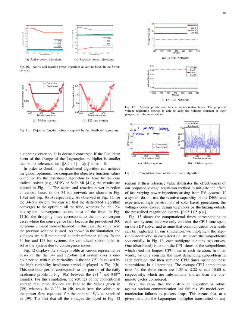
Fig. 10. Active and reactive power injections at various buses in the 34-busnetwork.

400 600 8000

0.05

0.1

Time horizon (min)

Obje

ctive function v

alu

e

Centralized

Distributed

(a) 34-bus system

400 600 8000.38

0.4

0.42

0.44

Time horizon (min)

Obje

ctive function v

alu

e

(b) 123-bus system

Fig. 11. Objective function values computed by the distributed algorithm.

a stopping criterion. It is deemed converged if the Euclideannorm of the change of the Lagrangian multiplier is smallerthan some tolerance, i.e., ‖λ[t+ 1]− λ[t]‖ < 1e− 6.

In order to check if the distributed algorithm can achievethe global optimum, we compare the objective function valuescomputed by the distributed algorithm to those by the cen-tralized solver (e.g., SDP3 or SeDuMi [41]); the results areplotted in Fig. 11. The active and reactive power injectionat various buses in the 34-bus network are shown in Fig.10(a) and Fig. 10(b) respectively. As observed in Fig. 11, forthe 34-bus system, we can see that the distributed algorithmconverges to the optimum all the time, whereas for the 123-bus system convergence occurs most of the time. In Fig.11(b), the dropping lines correspond to the non-convergentcases where the convergence fails because the pre-defined 300iterations allowed were exhausted. In this case, the value fromthe previous solution is used. As shown in the simulation, thevoltages are still maintained at their reference values. In the34-bus and 123-bus systems, the centralized solver failed tosolve the system due to convergence issues.

Fig. 12 displays the voltage profile at various representativebuses of the the 34- and 123-bus test system over a one-hour period with high variability in the the PPVi ’s caused bythe high-variability irradiance period displayed in Fig. 9(b).This one-hour period corresponds to the portion of the dailyirradiance profile in Fig 9(a) between the 781th and 840th

minutes. For this simulation, the settings of the conventionalvoltage regulation devices are kept at the values given in[39], whereas the V refi ’s in (4b) result from the solution tothe power flow equations for the nominal Pi’s as specifiedin [39]. The fact that all the voltages displayed in Fig. 12

780 790 800 810 820 830 840

1

1.02

1.04

1.06

Minutes

Volta

ge

Ma

gn

itud

e

Feeder

Bus 5

Bus 10

Bus 15

(a) 34-Bus Network

780 790 800 810 820 830 8400.98

0.99

1

1.01

1.02

1.03

1.04

Minutes

Vo

ltag

e M

ag

nitu

de

Feeder

Bus 7

Bus 67

Bus 99

(b) 123-Bus Network

Fig. 12. Voltage profile over time at representative buses. The proposedvoltage regulation method is able to keep the voltages constant at theirperspective references values.

400 600 8000

10

20

30

40

50

Time horizon (min)

CP

U tim

e (

s)

Cumulative

Distributed

(a) 34-bus system

400 600 8000

200

400

600

800

Time horizon (min)

CP

U tim

e (

s)

cumulative

distributed

(b) 123-bus system

Fig. 13. Computation time of the distributed algorithm.

remain at their reference value illustrates the effectiveness ofour proposed voltage regulation method to mitigate the effectof fast-varying power injections arising from PV systems. Ifa system do not use the reactive capability of the DERs andexperiences high penetrations of solar-based generation, thevoltages could exceed design tolerances by fluctuating outsidethe prescribed magnitude interval [0.95,1.05 p.u.].

Fig. 13 shows the computational times corresponding toeach test system; here we only consider the CPU time spenton the SDP solver and assume that communication overheadscan be neglected. In our simulation, we implement the algo-rithm iteratively; in each iteration, we solve the subproblemssequentially. In Fig. 13, each subfigure contains two curves.One (distributed) is to sum the CPU times of the subproblemswhich need the longest CPU time in each iteration. In otherwords, we only consider the most demanding subproblem ineach iteration and then sum the CPU times spent on thesesubproblems in all iterations. The average CPU computationtime for the three cases are 1.28 s, 3.33 s, and 19.69 s,respectively, which are substantially shorter than the one-minute cycles considered.

Next, we show that the distributed algorithm is robustagainst random communication link failures. We model com-munication failures as packets drops. This means that, at agiven iteration, the Lagrangian multiplier transmitted on any

11

380 390 400 410 420 4301.5

2

2.5

3

3.5

4

4.5

5

5.5

6

6.5

Time horizon (min)

CP

U tim

e (

s)

0

0.1

0.3

Fig. 14. Time it takes for Algorithm 1 to converge under the presence ofcommunication link failures.

particular edge could be lost with probability p, independentof all other transmissions. Figure 14 shows the average time ofconvergence needed over the day for the 34-bus network forp = 0, p = 0.1 and p = 0.3; convergence is always achieved.

Remark 1. The results displayed in Fig. 11 correspond to acentralized solution of (8); however, we also performed simu-lations using a centralized solver (SeDuMi) to obtain a solutionto (12). However, the algorithm failed to converge most ofthe time even for the 34-bus network. We suspect that sincethere are duplicated variables in (12), a naive implementationwould be rather inefficient; however, a more careful centralizedimplementation (using, e.g., an SOCP formulation) is likelyspeed up (12).

VII. CONCLUDING REMARKS

We proposed a convex optimization based method to solvethe voltage regulation problem in distribution networks. Wecast the problem as a loss minimization program. We showedthat under broad conditions that are likely to be satisfied inpractice, the optimization problem can be solved via its convexrelaxation. We then proposed a distributed algorithm that canbe implemented in a network with a large number of buses; wedemonstrated the effectiveness and robustness of the algorithmwith two case studies.

As noted earlier, the proposed voltage regulation methodis intended to supplement the action of conventional voltageregulation devices. In this regard, throughout the paper, weassumed that there is a separation in the (slow) time-scale inwhich the settings of conventional voltage regulation devicesare adjusted and the (fast) time-scale in which our proposedmethod operates. With respect to this, a research directionworthy exploring is to carefully consider the coupling acrossthe two time-scales and study the interplay between the opti-mal use of conventional voltage regulation devices in longertime-scales, and the use of our voltage regulation method inshorter time-scales. This would allow us to, e.g., study thetrade-offs between the location and number of conventionalvoltage regulation devices, and the location and number ofDERs and DRRs with capability of providing reactive power.

APPENDIX

Proof of Theorem 1: The first and third cases are clear.The interesting case to prove is to show that if the matrixW∗ has rank higher than 1, there is no rank-1 matrix W thatresults in a feasible solution.

The requirement that Qi< βi for i = 2, . . . , n is to ensure

that the reactive lower bound is in fact never tight for all thenodes in the network. Let h be the parent of i and k be a childof i. Since we assume that power always flow from parentsto children in the network, and from the angle constraint in(9), 0 ≤ θhi ≤ tan−1( bikgik ). Over this range, Qih ≥ 0. Thiscorresponds to the intuition that reactive power should flow upthe tree to support the voltage. Note the inductive line is verylossy in terms of reactive powers, therefore i might receiveor supply reactive power to k. The Qik is monotonic in θikstarting at θik = 0 until it reaches is minimum at an angleof tan−1( gikbik ). Let θik = min(tan−1( gikbik ), θik), then Qi =Qih +

∑k:k∈C(i)Qik ≥

∑k:k∈C(i)Qik ≥

∑k:k∈C(i) bik −

gik sin(θik) − bik cos(θ(θ)ik) = βi. Thus, if Qi< βi, the

lower bounds on the reactive power injections are never tight.To finish the proof we need to introduce some notations

from [22]. For a n bus network, let {θik} be the set of angleconstraints, one for each line. Then, the angle-constrainedactive power injection region is the set of all active powerinjection vectors that satisfy the line angle constraints, i.e.,Pθ = {p : p = Re{diag(vvHYH)}, |Vi| = 1, |θik| ≤ θik}.Let Fθ ⊂ R2n−2 be the Cartesian product region of then − 1 active line flow regions, then Fθ = Πi∼kFθ,ik. LetM ∈ Rn×2n−2 be a matrix with the rows indexed by thebuses and the columns indexed by the 2(n − 1) ordered pairof edges, i.e., if i is connected to k, both (i, k) and (k, i)are included; thus M[i, (k, l)] = 1 if i = k or i = l, andM[i, (k, l)] = 0 otherwise. M is a generalized edge to busincidence matrix, and Pθ = MFθ i.e., the power injectionregion is obtained by a linear transformation of the product ofline flow regions.

Similarly, Gθ is the product region of the n − 1 reactiveline flow regions. Then, for all (i, k), by stacking the Hik’sas defined in (11) into a 2(n− 1)× 2(n− 1) block diagonalmatrix H, i.e., H = diag({Hik}i∼k), we obtain a the globaltransform between F and G. The angle-constrained reactivepower injection region Qθ is given by Qθ = MGθ = MHFθ.

Since by construction the lower bonds on the reactive powerinjection are never tight, we can ignore them from now on.Let P be the feasible region of the original problem (6), thatis, P = {p : ∃v ∈ Cn, Pi = Tr(Aivv

H), |Vi| = 1, P i ≤Pi ≤ P i,Tr(Bivv

H) ≤ Qi, |θik| < θik,∀i ∼ k}. We canequivalently write P as P = M(Fθ ∩ FP ∩ FQ), where FPis the flow region satisfying the real power constraints, thatis, FP = {f ∈ R2n−2 : p = Mf , P i ≤ Pi ≤ P i}. FQ is theflow region satisfying the reactive power constraints, that is,PQ = {f ∈ R2n−2 : q = MHf , Qi ≤ Qi}. Since FP and FQare defined by linear inequalities, they are convex. However,Fθ is not.

Let S be the feasible region of the relaxed problem (8). Itturns out that S = M(convhull(Fθ) ∩ FP ∩ FQ), is convex,and contains P .

12

Now we need to define the Pareto-front of a set. Let X ⊂Rn, we say x ∈ X is Pareto-optimal if 6 ∃y ∈ X such thaty ≤ x with strict inequality in at least one coordinate. The setof Pareto-optimal points is called the Pareto-front of X , andlabeled O(X ). When minimizing a strictly increasing function,the optimal is always achieved in the Pareto-front. Thereforeto show the second statement in the theorem, it suffices toshow the following lemma.

Lemma 2. Suppose P is not empty, then P = O(S).

Suppose the lemma is true, then if the optimal solution ofthe relaxed problem (8) is of rank 2, then P must be empty.

The proof of this lemma is similar to Lemma 4 in [22].Let p∗ ∈ S be the optimal solution of the relaxed problem,f∗ ∈ convhull(Fθ) ∩ FP ∩ FQ its corresponding active flowvector and r∗ = Hf∗ be the corresponding reactive power flowvector. It suffices to show that if P ∗i > P i, then (f∗ik, f

∗ki) ∈

Fθ,ik for every k ∼ i. Once this fact is established, the rest ofthe proof is the same as the proof of Lemma 4 in [22]. Supposethat P ∗i > P i, but (f∗ik, f

∗ki) /∈ Fθ,ik for some k. Then there

exists ε > 0 such that (f∗ik − ε, f∗ki) ∈ convhull(Fθ,ik). Let(fik, fki) = (f∗ik − ε, f∗ki). Since

Hik

[−ε0

]= − ε

2bikgik

[b2ik − g2ikb2ik + g2ik

]< r∗,

Therefore (fik, fki) is a better feasible flow on the line (i, k),which contradicts the optimality of f∗.

REFERENCES

[1] “U.S.Department of Energy — Smart Grid,” http://www.oe.energy.gov/smartgrid.htm.

[2] “European technology platform for the electricity networks of thefuture,” http://www.smartgrids.eu.

[3] P. Carvalho, P. Correia, and L. Ferreira, “Distributed reactive powergeneration control for voltage rise mitigation in distribution networks,”IEEE Trans. Power Syst., vol. 23, no. 2, pp. 766–772, May 2008.

[4] A. Keane, L. Ochoa, E. Vittal, C. Dent, and G. Harrison, “Enhancedutilization of voltage control resources with distributed generation,”IEEE Trans. Power Syst., vol. 26, no. 1, pp. 252–260, Feb. 2011.

[5] C. Guille and G. Gross, “A conceptual framework for the vehicle-to-grid(v2g) implementation,” Energy Policy, 2009.

[6] G. Joos, B. Ooi, D. McGillis, F. Galiana, and R. Marceau, “The potentialof distributed generation to provide ancillary services,” in Proc. of IEEEPower Engineering Society Summer Meeting, Seattle, WA, 2000.

[7] D. Logue and P. Krein, “Utility distributed reactive power control usingcorrelation techniques,” in Proc. of IEEE Applied Power ElectronicsConference, Anaheim, CA, March 2001.

[8] Petra Solar. (2009) SunWave Pole-Mount Solutions. South Plainfield,NJ. [Online]. Available: http://www.petrasolar.com/

[9] SolarBridge Technologies. (2009) Pantheon Microinverter. SouthPlainfield, NJ. [Online]. Available: http://www.petrasolar.com/

[10] S. Boyd and L. Vandenberghe, Convex Optimization. Cambridge, 2004.[11] M. Prymek and A. Horak, “Multi-agent approach to power distribution

network modelling,” Integrated Computer-Aided Engineering, 2010.[12] S. Rumley, E. Kagi, H. Rudnick, and A. Germond, “Multi-agent ap-

proach to electrical distribution networks control,” in Computer Softwareand Applications, 2008. COMPSAC ’08. 32nd Annual IEEE Interna-tional, 2008, pp. 575–580.

[13] M. Baran and I. El-Markabi, “A multiagent-based dispatching schemefor distributed generators for voltage support on distribution feeders,”IEEE Trans. Power Syst., vol. 22, no. 1, pp. 52–59, Feb. 2007.

[14] K. Turitsyn, P. Sulc, S. Backhaus, and M. Chertkov, “Distributedcontrol of reactive power flow in a radial distribution circuit with highphotovoltaic penetration,” in Proc. of IEEE Power and Energy SocietyGeneral Meeting, 2010, Minneapolis, MN, July 2010, pp. 1–6.

[15] D. Villacci, G. Bontempi, and A. Vaccaro, “An adaptive local learning-based methodology for voltage regulation in distribution networks withdispersed generation,” IEEE Trans. Power Syst., vol. 21, no. 3, pp. 1131–1140, Aug. 2006.

[16] A. A. Aquino-Lugo, R. Klump, and T. J. Overbye, “A control frameworkfor the smart grid for voltage support using agent-based technologies,”IEEE Trans. on Smart Grid, vol. 2, no. 1, pp. 173 –180, March 2011.

[17] X. Bai, H. Wei, K. Fujisawa, and Y. Wang, “Semidefinite programmingfor optimal power flow problems,” Electrical Power and Energy Systems,2008.

[18] J. Lavaei and S. Low, “Zero duality gap in optimal power flow,” IEEETrans. on Power Syst., vol. 27, no. 1, Feb. 2012.

[19] B. Zhang and D. Tse, “Geometry of feasible injection region of powernetworks,” in In Proc. of Forty-Ninth Annual Allerton Conference,Monticello, IL, 2011.

[20] S. Sojoudi and J. Lavaei, “Network topologies guaranteeing zero dualitygap for optimal power flow problem,” in Proc. of IEEE PES GeneralMeetings, 2012.

[21] S. Bose, D. F. Gayme, S. Low, and M. K. Chandy, “Optimal powerflow over tree networks,” in In Proc. of the Forth-Ninth Annual AllertonConference, Monticello, IL, 2011.

[22] J. Lavaei, D. Tse, and B. Zhang, “Geometry of power flows in treenetworks,” in Proc. of IEEE PES General Meetings, 2012.

[23] B. Stott, J. Jardim, and O. Alsac, “DC power flow revisited,” IEEETrans. on Power Syst., vol. 24, no. 3, August 2009.

[24] M. Farivar, R. Neal, C. Clarke, and S. Low, “Optimal inverter var controlin distribution systems with high pv penetration,” in Proc. of the IEEEPower and Engergy Society General Meeting, 2012.

[25] M. Kraning, E. Chu, J. Lavaei, and S. Boyd. (2012) Messagepassing for dynamic network energy management. [Online]. Available:http://arxiv.org/abs/1204.1106

[26] N. Li, L. Chen, and S. Low, “Exact convex relaxation of opf for radialnetworks using branch flow model,” in in Prod. 2012 IEEE Third Inter-national Conference on Smart Grid Communications (SmartGridComm),2012, pp. 7–12.

[27] B. Zhang and D. Tse, “Geometry of feasible injection region of powernetworks,” http://arxiv.org/abs/1107.1467, 2011.

[28] L. Gan, N. Li, U. Topcu, and S. H. Low, “On the exactness of convexrelaxation for optimal power flow in tree networks,” in In Prof. 51stIEEE Conference on Decision and Control, Dec. 2012.

[29] N. Li, L. Gan, L. Chen, and S. H. Low, “An optimization-baseddemand response in radial distribution networks,” in in Proc. IEEESmart Grid Commun. Workshop: Design for Performance (GLOBECOMWorkshops), Dec. 2012.

[30] W. H. Kersting, Distribution system modeling and analysis. CRC Press,2006.

[31] A. Bergen and V. Vittal, Power System Analysis. Upper Saddle River,NJ: Prentice Hall, 2000.

[32] K. Zou, A. P. Agalgaonkar, K. M. Muttaqi, and S. Perera, “Distributionsystem planning with incorporating dg reactive capability and systemuncertainties,” IEEE Trans. on Sustainable Engergy, vol. 3, no. 1, 2012.

[33] E. A. J. Brea, “Simple photovaltic solar cell dynamic sliding mode con-trolled maimum power point tracker for battery charging applications,” inProceedings of the Twenty-Fifth Annual IEEE Applied Power ElectronicsConference and Exposition (APEC), Feb. 2010, pp. 666–671.

[34] R. E. Tarjan and M. Yannakakis, Simple linear-time algorithms to testchordality of graphs, test acyclicity of hypergraphs, and selectivelyreduce acyclic hypergraphs. Society for Industrial and AppliedMathematics, 1984.

[35] A. Y. S. Lam, B. Zhang, and D. Tse, “Distributed algorithms for optimalpower flow problem,” in Proc. IEEE 51st Annual Conf. on Decision andControl, 2012.

[36] H. Terelius, U. Topcu, and R. M. Murray, “Decentralized multi-agentoptimization via dual decompostion,” in in Proc. 18th World Congressof the International Federation of Automatic Control, 2010.

[37] S. Boyd, L. Xiao, A. Mutapcic, and J. Mattingley, Notes on Decompo-sition Methods. Stanford University, 2008.

[38] W. H. Kersting, “Radial distribution test feeders,” in Proc. of IEEEPower Engineering Society Winter Meeting, Columbus, OH, 2001.

[39] Distribution Test Feeder Working Group, “Distribution test feeders,”http://ewh.ieee.org/soc/pes/dsacom/testfeeders/index.html, 2010.

[40] National Renewable Energy Laboratory, “Solar radiation data,”http://www.nrel.gov/solar/, 2011.

[41] J. Sturm, “Using SeDuMi 1.02, a MATLAB toolbox for opti-mization over symmetric cones,” Optimization Methods and Soft-ware, vol. 11–12, pp. 625–653, 1999, version 1.05 available fromhttp://fewcal.kub.nl/sturm.