Optimal Distributed Photovoltaic Generation Capacity ... · Optimal Distributed Photovoltaic Generation Capacity: ... professional organizations such as the IEEE and ANSI. ... The

Optimal Distributed Photovoltaic Generation

Capacity: Puerto Rico Case Study Capstone Research Project

April 24, 2015

Daniel Schultz

Jennifer Baker

Michael Liu

Jeffrey Smith

Interdisciplinary Telecom Program

University of Colorado Boulder

Mark Dehus

Instructor

University of Colorado Boulder

Tomás Vélez Sepúlveda

Electrical Engineer

Puerto Rico Electric Power Authority

Abstract— The integration of renewable sources of energy has

become one of the most important energy policies worldwide.

With ever-evolving grid and energy policies, one of the major

challenges experienced by the electric utility companies today is

maintaining reliability and high efficiency of the assets on the

grid. Renewable sources of energy provide environmental and

economic advantages; however due to the dynamics of the

natural resources, these technologies can also affect the power

systems’ operations. One of the key elements under high-

distributed generation deployment is determining the maximum

capacity that existing power systems can handle. How much

capacity of photovoltaic distributed generation can be integrated

into a distribution feeder power system while maintaining the

voltage profile within the limits established by ANSI C84.1-2011?

To answer this question, we did a case study to address the

following: distribution feeder model representation, data

measurements, and Python simulations and analysis. For this

case study, we conclude that an average photovoltaic distributed

generation capacity value of 115% of the local demand can be

accommodated at each consumer load point.

Keywords—photovoltaic; distributed generation; maximum

capacity; optimal; feeder; efficiency

I. INTRODUCTION

The integration of renewable sources of energy has become one of the most important energy policies worldwide. Recently, many states have adopted Renewable Portfolio Standards (RPS) mandates, which require the integration of large percentages (i.e. 33%, 25%, and 20%) of renewable sources of energy [1]. Although there are great advantages that come along with such integration (e.g. diversification of utilities’ generation portfolio, reduction of electrical energy losses in the transmission and distribution stages, reduction of carbon dioxide emissions, and customer’s onsite generation opportunity through interconnection regulations, among others), the interconnection of these sources can also impact the distribution systems in a significant way. The most common impacts in a distribution system can be classified within the voltage regulation profiles and protection schemes of distribution feeders.

Moreover, since the distribution infrastructure of existing power systems was not designed to integrate flow of electrical energy from the load side upstream to the distribution substation or other loads, the power systems’ operations, along with the varying dynamics of natural resources like wind and solar, bring along many other challenges that electric utility companies need to overcome to comply with the RPS and meet the established goals.

A. Statement of the Problem

With ever evolving grid and energy policies, one of the major challenges experienced by the electric utility companies today is maintaining reliability and high efficiency of the assets on the grid [2]. Today’s focus on providing a better electrical energy service to clients, and reducing or modifying the electrical energy consumption’s behavior lead to the optimization of the power system’s operation. However, to achieve this, it is important to understand that the characteristics of a power system are particular for each case and consequently, the challenges that come along can vary significantly.

In particular, small isolated power systems, such as those found on an island, have the largest challenges to maintain stability. Mainly, this is because these systems are not interconnected and do not rely on backup generation. Typically, small islands like Hawaii and Puerto Rico have this type of electric infrastructure and the operators need to generate the amount of energy that is needed to cover the energy demand and losses. When comparing an islanded power system with a large interconnected power system, a disadvantage of relatively low inertia and high sensitivity to frequency variations can be experienced. To mitigate significant frequency variations, it is extremely important to avoid mismatch between the amount of energy that is being generated and the amount of energy that is being demanded by the loads plus the energy losses along the way. Since an islanded power system does not rely on external generation backup, the consequences of having a significant mismatch between generation and demand can cause a total system collapse.

2

To maintain power system stability, a balance between energy generation and demand must exist. For many years, electric utility companies, without a means to control demand, have had to estimate the amount of energy that will be demanded by the system loads based on power flow analysis and historical data. However, with the integration of distributed generation (DG), the two main variables (energy generation and demand) that determine the frequency magnitude in a power system can vary without utility control, and the complexity to maintain power systems stability increases significantly. Therefore, in order to comply with current energy policies, especially when large amounts of integrated renewable sources of energy are introduced into existing islanded power systems, it is crucial to know the limits of how much energy can be integrated coming from intermittent renewable sources like solar photovoltaic (PV). This must be done without affecting the power quality of the system as established in the standards developed by professional organizations such as the IEEE and ANSI. With this information, electric utility companies can integrate adequate amounts of aggregated capacity of DG into distribution feeders while maintaining a safe and reliable service to all clients without significantly affecting the power quality.

B. Research Question

What is the optimal PV DG systems’ allocation to maximize integration of these sources in a distribution feeder while maintaining the voltage profile within the limits established by ANSI C84.1-2011?

1) Distribution Feeder Model Representation

The challenges and impacts that come along when

integrating renewable sources of energy into existing power systems depend on its particular characteristics. One of the major challenges for PV interconnection is a low demand and high generation scenario, where the voltage limits can be exceeded, potentially causing equipment malfunction or damage [3]. For instance, this type of issue can occur on a very sunny day during a low demand period such as in the middle of the day in a residential area, when people are not at home. This low demand, high generation scenario causes mathematical anomalies on that extreme end of the model [4]. Another problem found in all renewable power generation sources, including PV, is energy generation variation. Any natural event that effectively decreases the solar input into the PV, such as a cloudy day, sandstorm, or haze decreases the amount of power generated by the system [4]. These fluctuations make it difficult to create an accurate model from statistics alone. Another problem that is inherent in any distribution system is feeder length; the voltage losses increase as the distance from the substation transformer increases [5].

A current 8.32 kV distribution feeder (see Fig. 1 [6]) from Puerto Rico was analyzed in this paper to collect the technical data required to complete the model. The data set included primary voltage level, impedance and distance values of all the conductors per phase, load current meters’ data, and equipment rating values.

2) Data Measurements

To complete the model representation and simulate the

power flow to analyze the voltage profile along the distribution feeder, real load and generation profiles were used. It is known that, among other characteristics, the type of dominating loads that the distribution feeders supply energy to is what establishes the energy demand behavior. For example, a residential load type feeder has a higher energy demand at nighttime while a commercial load type feeder has a higher energy demand during the day (especially during the weekdays). On the other hand, these behavior characteristics can be different during the weekends, with larger usage throughout the day and night in residential areas and less usage in commercial and business zones. Although demand behaviors can vary throughout the days of the week and with the seasons of the year, PV DG only depends on solar radiation and other climate conditions to generate electrical energy. Therefore, to obtain energy demand and generation values, real data measurements were collected through current distribution profilers (primary line current metering equipment) and nominal PV capacity values were considered.

3) Simulation Results

Electric utility companies that have RPS and

interconnection regulations for transmission and distribution systems need to perform different sets of analyses to ensure safe and reliable interconnection of DG while maintaining the required power quality to all consumers. Such evaluations may include voltage regulation, short circuit, flicker, protection coordination, power quality harmonics, and overall power systems analyses. Although all of these analyses are important and play their corresponding roles, the voltage regulation impacts are the most common at the distribution system. The voltage regulation impact may be experienced as

Fig. 1 – 8.32 kV Distribution Feeder in Puerto Rico

3

an overvoltage at the zone near the DG site and/or as a significant voltage variation (e.g. 3%) when comparing DG maximum generation scenario with DG minimum generation scenario (i.e. renewable source not available).

Historically, it has been demonstrated that there are different variables that can contribute directly towards the impact of voltage regulation in a distribution feeder. The first contributor is the voltage level of the distribution system. Depending on the voltage level at which the distribution feeders operate, the voltage regulation robustness can be classified. The higher the voltage, the stronger and more effective voltage regulation is obtained. With a better voltage regulation, less voltage variations can be experienced and more DG capacity can be integrated. The second contributor is the capacity and technology of the DG. Since there are different technologies available to be used as DG energy sources, such as wind, solar, biomass, and even internal combustion micro turbines, due to their different generation profiles (especially those that use renewable and intermittent sources of energy), energy management and supply is directly impacted. The third contributor is the distribution feeder loads’ energy demand profile. This variable determines the worst-case scenarios (e.g. maximum/minimum demand with maximum/minimum generation profile). In the scenario of maximum demand with maximum/minimum generation, significant voltage change conditions can be experienced. Since maximum demand also implies maximum voltage drop along the distribution feeder, DG integrated at the end of the distribution feeder can be provided with the lowest voltage magnitude due to the impedance of the conductors from the distribution substation to the DG’s point of interconnection (POI). Therefore, when comparing the voltage at the POI when the DG is providing maximum generation with the voltage when the DG is not generating energy, it can have a difference of more than what is required or recommended by interconnection regulations and utility practices (i.e. 3% – 5%).

On the other hand, in the scenario where there is minimum demand with maximum generation profile, overvoltage conditions can be experienced. Since power flows from higher voltage magnitude nodes to lower voltage magnitude nodes, the power export from DGs can increase the voltage magnitude near its POI. Moreover, in a minimum demand scenario, the voltage drop is lower than in a maximum demand scenario. Therefore, higher voltage magnitude is provided by the electric utility companies. Consequently, if the DG’s voltage increase is added, the voltage magnitude can exceed the voltage limits established by the ANSI C84.1-2011 standard.

The ANSI C84.1 is the standard that establishes the nominal voltage ratings and operating tolerances for 60 Hz electric power systems above 100 volts [7]. For this research, secondary voltage has an upper limit of 126 V (see Fig. 2 [7]).

The main purposes of the standard are:

Promote a better understanding of the voltages associated with power systems and equipment.

Achieve practical and economical design and operation.

Establish uniform nomenclature in the field of voltages.

Promote standardization of nominal system voltages and ranges of voltage variations for operating systems and equipment voltage ratings and tolerances.

Provide a guide for future development and design of equipment to achieve the best possible conformance with the needs of the users and with respect to choice of voltages for new power system undertakings and changes in older ones [7].

Currently, very few commercially available software tools can be used to simulate the impact of DG integration into existing distribution systems. SynerGEE Electric has the capacity to simulate the steady state impact of PV DG and provides the overall results for the voltage regulation profile. It can also calculate the short circuit current values and impedance values. Since the majority of power quality issues and DG impacts into distribution feeders are experienced on the voltage regulation and protection schemes, SynerGEE Electric is a suitable and convenient tool to validate the base configurations of all simulated scenarios.

4) Quantifying Maximum PV DG Capacity

To quantify the maximum amount of PV DG capacity that

can be integrated into distribution feeders is not an easy task since it varies according to the specific characteristics of the electrical infrastructure, load demand profile and generation capacity and technologies. The data collected from the distribution feeder provided us raw measurement data from each phase of the system. Therefore, analyses of data to determine the different scenarios that have to be simulated were completed. The simulation results from SynerGEE Electric further provided us with different scenarios that helped make sense of the data, putting the data in context and demonstrating the impacts of DG (i.e. how it affects voltage profile and frequency characteristics). In order to answer the final question of how much DG capacity can be integrated, we compared the simulation results to the ANSI C84.1-2011 standard. Through calculations, boundaries and thresholds, sets of conditions were identified in which DG capacity must be capped to satisfy power quality requirements defined by ANSI C84.1-2011. Different variables were studied (e.g. voltage, energy demand and POI) so the most sensitive

Fig. 2 - ANSI C84.1-2011 Voltage Limits

4

variable can be identified. The initial assumption is that the voltage profile is most sensitive to DG integration. A Python tool was developed for data analysis and calculation for this particular project.

II. LITERATURE REVIEW

Today’s electric distribution systems have evolved over many years in response to load growth and changes in technology. The largest single investment of the electric utility industry is in the distribution system [8]. Although there are quite a few types of equipment available to contribute in the conversion of existing power systems into smart grids, most of the existing power infrastructure lack communication facilities as they are needed to control and manage both energy demand and generation from DG of renewable sources. Without communication and control, the penetration of DG on most circuits will be limited [8]. Although the increase of the hosting capacity of lines is one of the key elements under high DG deployment, the available measurements to attend this situation have proven to be costly or inconvenient to the end users [9][10]. Thus, the first decision-making step should be the calculation of the maximum DG capacity [11].

The impact of DG is increased within micro-grids and islanded systems. A micro-grid is a cluster of loads and micro-sources operating as a single system providing power to its local area. One of the most important features of micro-grids is that they can independently operate in an islanded mode without connecting to the distribution system when power system faults or blackouts occur [12]. A major concern of a micro-grid or islanded system in stability. The stability of a micro-grid is its ability to return to normal or stable operation after having been subjected to some form of disturbance. Conversely, instability means a condition denoting loss of synchronization or falling out of normal operation [13].

Distribution feeders are conventionally treated as a load with power flowing in one direction, from the substation to the end users. Conventional over-current protection is designed for radial distribution systems with unidirectional flow of fault current. However, connection of DGs into distribution feeders convert the singly fed radial networks to complicated ones with multiple sources [14]. Unlike large renewable energy generation facilities whose connection to the power grid can be monitored and controlled, private residential PV generation cannot be controlled in most cases by the utility company. This poses a unique challenge in maintaining stability.

This research contributes to the advancement of the body of knowledge by providing an evaluating software tool that can be used by electric utility companies to determine how much PV DG capacity can be integrated into a distribution feeder based on the load profile and DG’s POI without the need of applying restrictive safety measures to prevent distribution feeders’ negative impacts.

III. RESEARCH METHODOLOGY

A distribution feeder model was created using data from a current distribution feeder in Puerto Rico to represent an islanded power system accurately. Puerto Rico Electric Power Authority (PREPA) has a distribution system composed of an electric infrastructure with voltage levels ranging from 4.16 kV to 13.2 kV. Being a small power system, it contains

particular and challenging characteristics that are suitable for this research focus. Therefore, general operations data were requested and analyzed to understand the particular dynamic operations of this islanded distribution system. Since the impact of DG capacity depends on the specific feeder’s characteristics, a complete circuit trace was completed to gather conductor’s impedance and length data, protection equipment ratings, and voltage regulation devices’ information.

In order to make power flow models mirror real world conditions, load profiles were collected. To accomplish this, real data measurements were collected through Amcorder current distribution profilers (primary line current metering equipment). The Amcorder can record load demand data on systems that operate at voltages up to 69 kV and currents from 1 A to 1000 A. In addition, it can collect up to 64,000 data points at 1 to 60 second intervals before the data must be collected and the unit reset.

Data were collected at two strategic points along the distribution feeder. These specific points include the start of the feeder at the distribution substation, to measure the total current, and downstream at the point where the feeder splits into multiple branches. Data were collected on the particular distribution feeder in Puerto Rico for two months. Softlink, the software application that allows the user to download, view, graph, and import data from the Amcorder were used to collect the energy demand data. The data collected were used to create a simulated representation of the demand behavior of the distribution feeder.

SynerGEE Electric software from the GL-Group was used to pull together feeder data such as conductor type and length. Together with the current data collected from the field, the data were compiled for use in the distribution feeder model representation in the simulations. To calculate the impedances for each section, Ohm’s law was used. The detailed data for the distribution feeder model used were obtained from SynerGEE. The data set includes conductor type, conductor length and type, and the service transformers represented as connected kVA. The feeder is mapped into nodes and loads, but only the nodes with service transformers are connected to consumer loads that can interconnect PV systems. A load can be categorized into two types: conductor loads (impedance) of sections that interconnect two nodes and consumer loads (service transformers’ energy demand) that connect to ground.

Along with the distribution feeder topology, the model was created with the data provided by SynerGEE and the load data provided by Softlink and input into a text file for simulation and analysis. Analysis of the data required the creation of a Python tool that performs power flow calculations quickly from large amounts of data. Python was chosen to develop the tool because it is relatively easy to work with, whether to develop new tools or integration with existing ones [15]. In addition, “although Python is a general purpose programming language, some features of Python are especially suited for high-performance scientific computing and solving engineering problems” [16]. From the Python tool calculations, a minimum and maximum base case was established (no PV systems interconnected) using data from a minimum demand period and a maximum demand period, respectively.

5

In the development of the Python tool, the first step that was taken was the development of use cases. A use case is a high-level description of how a user would use and interact with the Python tool. Two use cases were developed. The first used the Python tool to determine how the addition of a single PV source at a specific location within the feeder would affect the voltage profile of the feeder. The second used the tool to determine, given a specific feeder, the optimal distribution of PV systems’ capacities within the feeder to find maximum amount of PV generation that could be integrated without a violation to the ANSI C84.1-2011 standard.

In both cases, the Python tool provided a detailed model of the feeder in its current state. The Python tool was designed to interpret input from the user to create a model of any feeder configuration. The approach taken was to break up a feeder into nodes and loads. A load represents one of two things within the feeder: the specific type and length of conductor and the consumer load. A consumer load is a representation of a group of homes and businesses served by the feeder through a step down service transformer. A node represents any point where the current splits. In this way, through object-oriented programing, the Python tool can be provided a list of loads with their corresponding impedances and start and end nodes. The Python tool then interprets this information to learn the configuration of the given feeder.

A function was developed in the Python tool that would be able to provide the impedance of a section of distribution cable based on its type and length. This was accomplished by accessing a database that houses impedances’ characteristics of known cable types. With the provided conductor type and length, the Python tool is able to determine the impedance of each section. The Python tool then had the impedance of each load of the feeder, the configuration of how the loads are connected and the voltage of the substation powering the feeder.

In order to obtain the voltage profile of the feeder, the voltages of each node in the feeder needed to be determined. The most effective way to do this task was to solve simultaneously for all the unknown voltage values at the same time using matrices, and the Python tool generated x unique algebraic equations for x unknown node voltages. The needed equations were derived by nodal analysis of each node using Kirchhoff’s current law in which the sum of all current entering and exiting a node must equal zero. An algorithm was developed to create the needed equation for each node. Each equation is made up of three specific values. The first, named Xn where n is the node number, is the sum of all load inverse impedances connected at the node being analyzed. Second is the inverse impedance of each conductor load connected to the node. The last value was the amount of current generated by PV generation at the node. These values became the coefficients of the unknown node voltages within the equation. The values of each equation vary based on the impedance of the loads and the feeder configuration. Once equations for each node were derived, the Python tool solved for the voltage of each node within the feeder (see Fig. 3).

To introduce PV generation into the feeder, the PV system at a node is simulated as a current source. The current from a PV system is introduced at the node of any consumer load. This changes the amount of current supplied by the feeder into the consumer load and thus alter the voltage profile of the

feeder. PV systems introduced by the user would be given in the kW value and converted into the corresponding current value by the Python tool.

Once the Python tool was able to analyze feeder behavior based on a specific set of initial conditions, the output format of the Python tool was designed. Several different output choices were developed, and the first choice was a simple analysis of the feeder given the initial conditions. This allowed a user to input the feeder information with any desired PV generation and obtain the new voltage profile of the feeder; this also addressed the first use case. The output of the Python tool includes the voltages of each node, the current through all loads of the feeder as well as power supplied by the substation and distributed PV generation and power consumed by each load. A second choice would allow the user to select a specific node associated with a consumer load and the Python tool would increase the PV generation at that node until the voltage profile of the feeder violated the ANSI C84.1-2011 standard. The output of the Python tool is the same as the first choice with the addition of a second file created recording how the voltage of each node of the feeder changed as the PV generation at a single node was increased. This data were used to analyze how PV generation in one part of the feeder affects the rest of the feeder. The third option was developed to address the second use case and determine the optimal distribution of PV generation in order to maximize PV generation within the feeder. In this option the Python tool makes an initial analysis of the feeder and then starts to add PV generation at each consumer load based on a percentage of each loads’ initial power consumption. The percentage is increased at all consumer loads until the ANSI C84.1-2011 standard is violated, and then the percentage is increased at individual consumer loads until the maximum PV generation is determined. The output from the Python tool would provide the amount of PV generation at each consumer load, in kW, as well as the total PV generation within the feeder and PV penetration of the feeder. The data from several different scenarios were collected and analyzed.

Zxy

y

PVy

zx

w

Zyz

Zy0

Zyw

I1

I 2

I3

I4

IPVy

I5

Node y

I1 – I2 – I3 – I4 = 0

I1 – I2 – I3 – (I5 -IPVy) = 0

(Vx - Vy) – (Vy – Vw) – (Vy – Vz) – (Vy – 0) + PVy = 0

Zxy Zyw Zyz Zy0

Vx/Zxy – Vy/Zxv – Vy/Zyw + Vw/Zyw – Vy/Zyz + Vz/Zyz – Vy/Zy0 + PVy = 0

(1/Zxy + 1/Zyw + 1/Zyz + 1/Zy0)Vy – (1/Zxy)Vx – (1/Zyw)Vw – (1/Zyz)Vz = PVy

XyVy – (1/Zxy)Vx – (1/Zyw)Vw – (1/Zyz)Vz = PVy

For Matrix equation

Coefficient for Node being analyzed = Xn

Coefficient for all Nodes directly connect to Node being analyzed

-1/(impedance between them)

Fig. 3- Algorithm derivation based off nodal analysis

6

For the purpose of the Python tool’s calculations, text files were prepared to represent the feeder, where each line in the file represents a load. The impedance of a conductor load is calculated by the conductor type and length. A database was further queried to obtain the unit length impedance value for the particular conductor type. On the other hand, to derive the impedance value of the consumer loads, additional calculations are performed. The calculation is based on Ohm’s law where impedance is obtained as voltage divided by current at that node. Since the substation voltage and the current values in each conductor load were available, voltage drop was calculated in each conductor load to derive voltage at each consumer load, and then current flowing to the consumer load was used to derive the impedance. Polar to rectangular conversion was applied during the process since SynerGEE provided current values in polar format and the Python tool uses impedance values in rectangular format. The calculations were done for all three phases and for both minimum and maximum demand simulations from SynerGEE.

Python tool’s voltage calculations were achieved using known power and current values in Ohm’s Law. To solve for the voltages, matrix math was applied with x number of rows for x number of variables to be solved. To quantify optimal PV generation capacity integration using Python, the data set was analyzed with several power flow techniques such as nodal analysis and circuit reduction. For this, Thevenin’s equivalent circuit configuration was used with a +5% nominal voltage value at the circuit source (i.e. 126 V on a 120 V base) and the corresponding equivalent circuit impedance. By iteration of the PV generation at small interval increases until the ANSI C84.1-2011 standard was violated, an optimal amount of PV generation could be determined.

IV. RESEARCH RESULTS

To validate the Python tool’s calculations and results, SynerGEE was used due to its well-known industry use for power flow analysis. This software has the necessary utilities to import or build distribution feeders’ models, insert generation profiles based on technologies (i.e. PV sources), and provide the voltage profile results based on per-phase values. The software also has methods to simulate weather impacts on PV generation, facilities and load that may come into play for scenarios including a low demand, high generation setup that would represent the middle of a weekday on a sunny day in a residential area.

Therefore, with the complete distribution feeder’s mathematical model, the base case scenarios were simulated and compared with SynerGEE’s output reports. With a slight difference of less than 1%, the Python tool is considered to have the capacity of successfully performing power flow analyses. Moreover, the Python tool’s results for all scenarios, confirmed the voltage impacts’ hypothesis based on theory concepts and literature review.

To answer many of the questions that utility engineers have about PV DG impacts on distribution feeders, strategic scenarios were simulated. Therefore, the Python tool was adjusted to perform required calculations for different scenarios. Table 1 and Table 2 detail the results and key findings throughout the scenarios under maximum and minimum energy demand, respectively.

Table 1 – Maximum Demand Scenarios and Results

6. POI variation - PV allocation concentrated

near the end of the feeder

Voltage profile along the feeder exceeds

the ANSI C84.1 optimum upper limit by up

to 6 V for phase A, 12 V for phase B, and 4 V

for phase C)

Voltage drops as impedance increases from

the substation (9 V for phase A, 18 V for

phase B, and 8 V for phase C)

1. Base - Load allocation without PV

Voltage profile along the feeder maintains

below the ANSI C84.1 optimum upper limit

as in the base case but with less voltage

drop (7 V for phase A, 9 V for phase B, and

4 V for phase C)


near the substation

Similar effect to POI corresponding case and

PV allocation is proportional (1:1) to energy

demand



demand

Voltage profile along the feeder maintains

within 0.3 V of ANSI C84.1 optimum upper

limit (105 % of nominal voltage; 5,040 V)

3. Optimal (Goal) - Optimal PV allocation

(201.6 kW at phase A, 266.1 kW at phase B,

109.7 kW at phase C)


at the middle of the feeder

Voltage profile along the feeder varies with

distance from substation (i.e. as distance

and impedance increase, the higher the

voltage rises)

8. Demand variation - Doubled demand

with PV allocation concentrated at the

middle of the feeder


with PV allocation concentrated near the

end of the feeder

Case Results

Maximum Demand - Simulation Scenarios


with PV allocation concentrated near the

substation



demand

Maximum PV capacities decrease down to

73% for phase A, 75% for phase B, and 82%

for phase C as distance from substation

increases

2. Maximum single PV - Gradually increased

Table 2 – Minimum Demand Scenarios and Results


with PV allocation concentrated near

the substation

Similar effect to POI corresponding case

and PV allocation is proportional (1:1) to

energy demand


with PV allocation concentrated at the

middle of the feeder



energy demand


with PV allocation concentrated near

the end of the feeder



energy demand

Voltage profile along the feeder

maintains within 0.2 V of ANSI C84.1

optimum upper limit (105 % of nominal

voltage; 5,040 V)

4. POI variation - PV allocation

concentrated near the substation


maintains below the ANSI C84.1

optimum upper limit as in the base case

but with less voltage drop (7 V for phase

A, 4 V for phase B, and 3 V for phase C)


concentrated at the middle of the

feeder

Voltage profile along the feeder varies

with distance from substation (i.e. as

distance and impedance increase, the

higher the voltage rises)


concentrated near the end of the feeder


exceeds the ANSI C84.1 optimum upper

limit by up to 6 V for phase A, 8 V for

phase B, and 2 V for phase C)

Minimum Demand - Simulation Scenarios

Case Results

1. Base - Load allocation without PV

Voltage drops as impedance increases

from the substation (9 V for phase A, 8 V

for phase B, and 5 V for phase C)

2. Maximum single PV - Gradually

increased

Maximum PV capacities decrease down

to 73% for phase A, 69% for phase B, and

80% for phase C as distance from

substation increases

3. Optimal (Goal) - Optimal PV allocation

(201.6 kW at phase A, 266.1 kW at phase

B, 109.7 kW at phase C)

7

It is known that PV DG impacts on a distribution feeder depend on many factors, such as voltage level, load demand, POI with the grid, and PV penetration. However, with the Python tool’s capacity to analyze the feeders in such described way, the impacts caused by these factors can be quantified.

V. DISCUSSION OF RESULTS

The most common question that arises nowadays in the renewable sources of energy arena is: How much DG capacity can be integrated into an existing power system? To answer this question, the data that represents the existing power system’s infrastructure and demand and generation behaviors is needed. However, since DGs’ impacts depend on various factors, the quantified answer will vary according to the particular characteristics that are considered.

As described in previous sections of the paper, the Python tool obtains the distribution feeder’s data from the user and performs simultaneous equation calculations to determine the voltage values at all nodes. For instance, Fig. 4 shows how the distribution feeder’s voltage profile decreases as distance from the substation increases. It is also notable to add that since the distribution feeder is not balanced, the demands per phase vary through time.

1) How load demand affects PV DG penetration?

To examine how the amount of PV DG penetration gets

affected with different demand values, simulations under maximum and minimum demand were performed. For both scenarios, the Python tool determined that to maintain a voltage profile in compliance with the ANSI C84.1-2011 standard, an average PV DG capacity value of 115% of the local demand can be accommodated at each consumer load. This value will have the effect of supplying the amount of energy that is consumed by the corresponding loads connected at the nodes and the energy losses associated with the feeder conductors. Fig. 5 shows how the voltages along the feeder stay within the ANSI C84.1-2011 standard values when the PV DG capacity is distributed along the feeder, supplying the corresponding local loads.

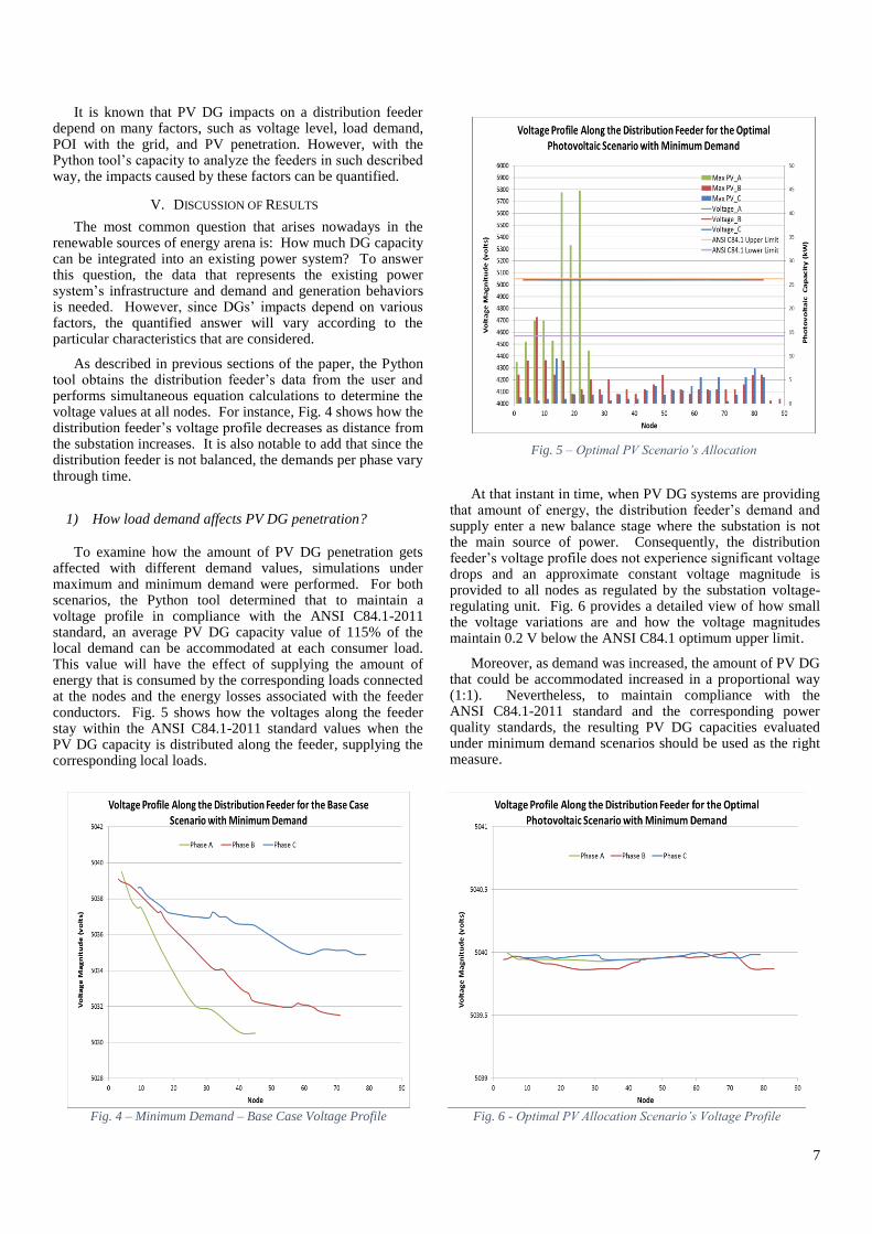
At that instant in time, when PV DG systems are providing that amount of energy, the distribution feeder’s demand and supply enter a new balance stage where the substation is not the main source of power. Consequently, the distribution feeder’s voltage profile does not experience significant voltage drops and an approximate constant voltage magnitude is provided to all nodes as regulated by the substation voltage-regulating unit. Fig. 6 provides a detailed view of how small the voltage variations are and how the voltage magnitudes maintain 0.2 V below the ANSI C84.1 optimum upper limit.

Moreover, as demand was increased, the amount of PV DG that could be accommodated increased in a proportional way (1:1). Nevertheless, to maintain compliance with the ANSI C84.1-2011 standard and the corresponding power quality standards, the resulting PV DG capacities evaluated under minimum demand scenarios should be used as the right measure.

Fig. 4 – Minimum Demand – Base Case Voltage Profile

Fig. 6 - Optimal PV Allocation Scenario’s Voltage Profile

Fig. 5 – Optimal PV Scenario’s Allocation

8

2) How PV DG’s POI affect the level of penetration?

To evaluate this factor, the total PV values determined in

the optimal PV allocation simulations for each phase were used. As seen previously in Fig. 5 and Fig. 6, the voltage profiles reach compliant states when PV DG is allocated in a distributed style accounting for an average of 115% of the local demand. However, when the same total amount of PV DG is concentrated in a single node, the voltage profiles change significantly (see Fig. 7).

At the beginning of the feeder, near the substation transformer, large concentrations of PV DG do not affect the overall voltage profiles since both sources (substation and PV DGs) are operating in parallel supplying local demand and downstream loads. Hence, the current can flow downstream affecting the voltage profile in a similar way as the base cases but with less voltage drops due to the demand that is being supplied locally where PV DG was concentrated. In this case, the advantage of reducing the power losses along the way gets lost because it still needs to travel from the sources to all loads in the feeder.

On the other hand, the exact same simulation characteristics were used but with PV DG concentrated at the end of the feeder. In this case, significant overvoltage conditions were observed. Throughout the whole feeder the voltage magnitudes exceeded the 105% upper limit established by the ANSI C84.1-2011 standard. Although PV DG supplies the local demand at the location where it is installed, this arrangement enabled an effect of “dynamics control”. Since the dynamics of current flow is from higher voltage magnitudes to lower voltage magnitudes, with PV DG connected at the end of the feeder without downstream loads, the voltage magnitudes in the feeder need to increase to accept the PV DG energy that is not consumed locally. The voltage magnitudes’ changes will depend on how much energy the PV DG is generating and the consumer loads are not absorbing (excess energy). Fig. 8 shows how the amount of PV DG that can be concentrated in a single feeder location reduces significantly as distance from the substation increases.

VI. CONCLUSIONS AND FUTURE RESEARCH

Determining the effects of renewable sources of energy interconnections with existing power systems is a complex task, and the Python tool developed for this research quantifies the steady state voltage regulation impacts on the distribution feeder studied, based on the particular characteristics considered. From the simulations discussed in the previous section of the paper, it can be concluded that to maximize the PV DG integration in a distribution feeder, the capacities of such systems should not exceed 115% of the local minimum demand values, and the allocation should be completed by distributing these PV DG capacities along the feeder.

Establishing energy policies to comply with the recommended practices derived in this research can increase the renewable sources of energy’s rate of deployment without affecting the power quality provided by electric utility companies. Moreover, it can take advantage of the benefits of onsite energy generation by reducing the distribution power losses, improving low voltage regulation (especially during maximum demand scenarios), providing the opportunity of interconnection to more consumers, and contributing to achieve better environmental practices to generate electrical energy. With these opportunities, research will also need to be done on how to implement this process, specifically how fairness can be taken into account when deciding if the capacity limits will be taken into account to approve interconnection requests, and how to address any design engineering and load balancing issues when these systems are brought online in quantity.

In regards to future expansion of this research, it is recommended to integrate evaluation of other compliance standards. The addition of short circuit and voltage flicker analysis would also add to the body of knowledge presented in this research, as well as the incorporation of capacitor banks and voltage regulators’ modeling as a check for voltage fluctuations that could assist with voltage adjustment. Another possibility for research involves expanding the capacity of the Python tool to analyze more than one feeder at a time,

Fig. 8 – Concentrated PV DG Penetration Profile

Fig. 7 - Minimum Demand Concentrated PV Voltage Profile

9

especially ones with complicated engineering. Policy and law research could also be done to research the feasibility of further PV penetration in all areas of the world, getting the world grid a step closer to sustainability.

Future research regarding PV distributed generation could focus on how to minimize voltage standard violations through engineering or monitoring capabilities. Smart grid technologies could offer a solution to many voltage issues, especially with voltage monitoring and current adjustment [17]. With a smart grid, the integrated communications system provides the operators with power flow information from these sources to the power grid. Along with the communications system, smart grids also include automated field equipment that can manage energy automatically and remotely depending on the different situations that may arise due to the natural complexities of sustainable energy sources. Smart grids enable power management companies to integrate sustainable energy sources into existing power systems by providing detailed flow of information, and increasing the field control with automatic energy management technologies, and study on this technology would advance the state of the art for this subject.

VII. REFERENCES

[1] FERC, “Renewable power & energy efficiency market:

Renewable portfolio standards,” Feb. 2010.

[2] R. Moghe, F. C. Lambert, and D. Divan, “Smart ‘stick-

on’ sensors for the smart grid,” IEEE Trans Smart Grid,

vol. 3, no. 1, pp. 241–252, Mar. 2012.

[3] I. T. Papaioannou and A. Purvins, “A methodology to

calculate maximum generation capacity in low voltage

distribution feeders,” Int. J. Electr. Power Energy Syst.,

vol. 57, pp. 141–147, May 2014.

[4] M. A. Mahmud, M. J. Hossain, and H. R. Pota, “Worst

case scenario for large distribution networks with

distributed generation,” in 2011 IEEE Power and

Energy Society General Meeting, 2011, pp. 1–7.

[5] V. V. Reddy, G. Yesuratnam, and M. S. Kalavathi,

“Impact of voltage and power factor change on primary

distribution feeder power loss in radial and loop type of

feeders,” in 2012 International Conference on Emerging

Trends in Electrical Engineering and Energy

Management (ICETEEEM), 2012, pp. 70–76.

[6] SynerGEE distribution feeder output. Puerto Rico

Electric Power Authority.

[7] National Electrical Manufacturers Association,

ANSI C84.1-2011.

[8] J. Paidipati, L. Frantzis, H. Sawyer, and A. Kurrasch,

“Rooftop photovoltaics market penetration scenarios,”

National Renewable Energy Laboratory, 2008.

[9] R. Passey, T. Spooner, I. MacGill, M. Watt, and K.

Syngellakis, “The potential impacts of grid-connected

distributed generation and how to address them: A

review of technical and non-technical factors,” Energy

Policy, vol. 39, no. 10, pp. 6280–6290, Oct. 2011.

[10] PV Grid, “Reducing barriers to large-scale integration of

PV electricity into the distribution grid,” D4.13,

Jul. 2013.

[11] M. Braun, T. Stetz, R. Bründlinger, C. Mayr, K.

Ogimoto, H. Hatta, H. Kobayashi, B. Kroposki, B.

Mather, M. Coddington, K. Lynn, G. Graditi, A. Woyte,

and I. MacGill, “Is the distribution grid ready to accept

large-scale photovoltaic deployment? State of the art,

progress, and future prospects: Distribution grid and

large-scale PV deployment,” Prog. Photovolt. Res.

Appl., vol. 20, no. 6, pp. 681–697, Sep. 2012.

[12] D. Velasco, C. L. Trujillo, G. Garcera, E. Figueres, and

O. Carranza, “Photovoltaic power management system

with grid connected and islanded operation,” presented

at the IEEE 20th International Symposium on Industrial

Electronics (ISIE 2011), 2011, pp. 1471–1476.

[13] P. Basak, S. Chowdhury, S. Halder nee Dev, and S. P.

Chowdhury, “A literature review on integration of

distributed energy resources in the perspective of

control, protection and stability of microgrid,” Renew

Sustain Energy Rev, vol. 16, no. 8, pp. 5545–5556,

Oct. 2012.

[14] S. P. Chowdhury, S. Chowdhury, and P. A. Crossley,

“Islanding protection of active distribution networks

with renewable distributed generators: A comprehensive

survey,” Electr Power Syst Res, vol. 79, no. 6,

pp. 984–992, Jun. 2009.

[15] D. M. Beazley, “Scientific computing with Python,”

presented at the Astronomical Data Analysis Software

and Systems IX, San Francisco, CA, 2000, vol. 216,

p. 49.

[16] S. Koranne, Handbook of open source tools. Boston,

MA: Springer, 2011.

[17] C. J. Mozina, “Impact of smart grid and green power

generation on distribution systems,” in Innovative Smart

Grid Technologies (ISGT), 2012 IEEE PES, 2012,

pp. 1–13.

Documents

Optimal Distributed Photovoltaic Generation Capacity ... · Optimal Distributed Photovoltaic Generation Capacity: ... professional organizations such as the IEEE and ANSI. ... The