Embed Size (px)
Citation preview

WP/07/135
An Oil and Gas Model
Noureddine Krichene


© 2007 International Monetary Fund WP/07/135
IMF Working Paper
African Department
An Oil and Gas Model
Prepared by Noureddine Krichene1
Authorized for distribution by Benedicte Vibe Christensen
June 2007
Abstract
This Working Paper should not be reported as representing the views of the IMF. The views expressed in this Working Paper are those of the author(s) and do not necessarily represent those of the IMF or IMF policy. Working Papers describe research in progress by the author(s) and are published to elicit comments and to further debate.
This paper formulated a short-run model, with an explicit role for monetary policy, for analyzing world oil and gas markets. The model described carefully the parameters of these markets and their vulnerability to business cycles. Estimates showed that short-run demand for oil and gas was price–inelastic, relatively income–elastic, and was influenced by interest and exchange rates; short-run supply was price–inelastic. Short-run price inelasticity could be a source for high volatility in oil and gas prices, and could confer to producers a temporary market power. Being simultaneous and incorporating interest and exchange rates, the model could be useful in short-term forecasting of oil and gas outputs and prices under policy scenarios. JEL Classification Numbers: C23, E40, E50, Q41, Q43 Keywords: Crude oil, demand, elasticity, exchange rate, impulse response, interest rate,
monetary policy, multiplier, natural gas, oil shock, supply. Author’s E-Mail Address: [email protected], [email protected],
1 The author expresses deep gratitude to Abbas Mirakhor, Abdoulaye Bio-Tchané, Geneviève Labeyrie, Anne-Marie Gulde-Wolf, Hans Weisfeld, Saeed Mahyoub, reviewers from RES and FAD, and Ibrahim Gharbi from Islamic Development Bank for their help with this paper.

2
Contents Page
I. Introduction ............................................................................................................................3
II. Modeling Demand and Supply of Crude Oil and Natural Gas .............................................5
III. Short-Run Demand and Supply Analysis ............................................................................8 A. Short-Run Crude Oil Demand Elasticities ................................................................9 B. Short-Run Natural Gas Demand Elasticities...........................................................14 C. Short-Run Crude Oil Supply Elasticities ................................................................17 D. Short-Run Natural Gas Supply Elasticities.............................................................18
IV. Simulation of the Model and Multiplier Analysis .............................................................19 A. Simulation of the Annual Model: Sample 1970─2006...........................................19 B. Simulation of the Quarterly Model: Sample 1984Q1─2006Q2..............................20 C. Multiplier Analysis..................................................................................................22
V. Structural Vector Auto-Regression Analysis......................................................................23
VI. Conclusions........................................................................................................................24 Tables 1. Crude Oil and Natural Gas: Short-Term Demand and Supply Elasticities..........................10 2. Multiplier Analysis ..............................................................................................................23 Figures 1a. Ratio of Natural Gas to Crude Oil Output, 1970-2006 ......................................................15 1b. Ratio of Natural Gas to Crude Oil Price, 1970-2006.........................................................15 2. Annual Simulation of the Oil and Natural Gas Model, 1970–2006 ....................................21 3. Quarterly Simulation of the Oil and Natural Gas Model, 1984Q1–2006Q2 .......................22 4. Annual Structural VAR: Impulse Responses.......................................................................25 5. Quarterly Structural VAR: Impulse Responses ...................................................................25 References................................................................................................................................29

3
I. INTRODUCTION
Recent oil and gas markets were marked by high price volatility, with oil prices hitting a record peak of US$78 per barrel in July 2006, and then suddenly falling by about 25 percent toward the end of 2006. These developments may be linked to monetary policy stance. Indeed, nominal interest rates in most industrial countries fell to lowest post-war levels during 2003, resumed a slow upward move, and then paused in 2006. Hence, expansionary, then accommodative, monetary policy seemed to have caused strong world economic growth during 2002–2006, and in turn high pressure on oil and gas markets. Rising oil and gas prices might ignite inflation and cause recession. Yet, despite the macroeconomic importance of world oil and gas markets, little has been done in modeling world demand and supply for crude oil and natural gas, or in exploring the role of monetary policy in these markets.2
On the demand side, most of demand studies have dealt with domestic demand for energy products, or sometimes, a group of countries’ demand for energy products (Balestra and Nerlove (1966), Pindyck (1979), Pesaran, et al. (1998), and Gately and Huntington (2002)) with no explicit role for monetary policy. On the supply side, most of the studies followed Fisher (1964) seminal work, concentrating on the supply of proven reserves of oil or gas instead of the supply of oil or gas output. Besides being country specific, Fisher’s model formulated the supply process, essentially from an engineering perspective, in three equations defined as wildcatting, success rate, and discovery rate equations, and did not have a direct output–price relation, as traditionally suggested by economic theory that would estimate directly supply–price elasticity. Besides mis-specification, parameters from these country-specific energy demand or supply studies are not necessarily applicable to world oil and gas markets characterized by heterogeneous countries at different stages in economic development and with different endowments in oil and gas resources.
This paper built a short-term model for world oil and gas that can explain oil and gas prices, with an explicit role for monetary policy.3 By incorporating the natural gas component, the model could be highly relevant for the hydrocarbons industry and useful in many applications, including short-term forecasting under scenarios for exogenous variables, evaluating monetary policy implications, and computing impulse response to shocks.
2 In view of full integration of capital markets, interest rates are reliable and readily available market indicators of underlying world demand conditions. A world measure for fiscal stance, however, is not available, and would be difficult to compute on a time series basis. For this reason, interest rates are highly relevant in explaining world oil and gas demand.
3 Long-run analysis is crucial for deeper understanding of oil and gas markets, and for energy policy design. In particular, long-term elasticities tend to be higher than short-term elasticities (Krichene, 2002). However, for reason of space, long-term modeling has not been addressed in this paper.

4
Demand and supply models are typically simultaneous equations models given the simultaneous determination of prices and quantities; namely prices are determined not only by suppliers, but also by consumers. The demand and supply equations are specified in structural form, according to traditional economic theory, defining aggregate demand by variables which are typically demand variables (e.g., prices, world income), and supply by variables which are typically supply variables (e.g., prices, world proven reserves).4 With regard to gas, special effort was given to estimating linkage with oil via cross-oil price elasticity.5 The reason for this linkage stemmed from the fact that the first oil shock in the fall of 1973, and subsequent oil shocks, might have caused considerable impact on the structure of demand and supply of natural gas; the latter is a close substitute to oil in may uses and can be directly influenced by developments in oil markets.
The paper has carefully analyzed the effect of monetary variables, namely the interest rate, given here by the LIBOR (London Inter-Bank Offered Rate, six–month U.S. dollar rate), and the U.S. nominal effective exchange rate (NEER), on world demand for oil and gas.6 The inclusion of these variables stemmed from the notion that monetary policy might have a significant effect on oil and gas markets, and therefore, it became necessary to analyze the relationship between interest and exchange rates and oil and gas markets.7
4 While this paper studied the impact of real GDP growth on oil demand and prices, the reader should be aware of a large body of literature which analyzed the effect of oil prices on real GDP, and which outgrew following the seminal work of Hamilton (1983). See also Hamilton (2003) and the review article by Jones, et al. (2004). It should be noted, however, that a relationship between oil price and real GDP, estimated at a country level, cannot be extended straightforwardly to world economy as changes in oil and gas prices affect differently net energy surplus and deficit economies.
5 Erickson and Spann (1971) modeled oil and gas as joint products and allowed for cross─oil price elasticity in the discovery equation for natural gas.
6 Bernanke, et al. (1997) have dealt with the role of monetary policy and the effect of an oil shock in a vector auto-regression (VAR) framework. While their model showed that most of the real GDP contraction was caused by ensuing tightening of monetary policy following an increase in oil price, it did not dealt with reverse causation from a monetary shock to oil prices, so relevant for explaining episodes in oil prices, including oil price trends observed in 1982–86 and 1999–2006. Furthermore, their model was essentially country–specific, and obviously its results cannot be extrapolated to world economy, as an oil shock may work differently at the level of world economy. Disagreeing with Bernanke, et al. (1997), Hamilton and Herrera (2004) contended that an oil shock, and much less monetary policy responsiveness to an oil shock, which caused ensuing economic recessions. As regards exchange rate, it may be noted that inclusion of this variable in an oil model is not a novelty of this paper. For instance, Amano and van Norden (1998) claimed that oil price shocks could be a dominant source in real exchange changes. 7 Dhal and Duggan (1998) have suggested inclusion of interest rate in the supply equation, as this variable has a significant effect on the cost of investment in the oil of gas industry. For the sake of simplicity, this paper has omitted interest and exchange rates on the supply side, and concentrated on their effect on the demand side.

5
To ascertain robustness of parameters, estimation was done on annual data for 1970–2006, and quarterly data for 1984Q1–2006Q2. The findings of the paper showed that short-run demand for oil was highly price-inelastic, with price elasticity ranging between -0.01 and -0.04. Demand for gas was also highly price inelastic, with price elasticity ranging between -0.01 and -0.11. Oil supply was also highly price inelastic, with price elasticity ranging between 0.01 and 0.02. Similarly, gas supply was highly price inelastic, with price elasticity ranging between 0.03 and 0.05. As implication of low price elasticities, any small excess demand or supply of oil or gas may require large movements in prices to clear markets for oil and gas. As most of the burden for clearing oil and gas markets falls on prices, price inelasticity becomes a source for volatility in oil and gas prices. Income elasticity ranged between 0.12 and 0.44 for oil, and 0.11 and 0.48 for gas, showing that energy demand was mainly driven by economic activity.
The paper demonstrated that oil and gas markets can be affected by shocks to monetary policy. Demand for oil and gas was significantly influenced by the interest rate (LIBOR) and the exchange rate (NEER). Interest rate semi–elasticity was estimated at -0.006 for oil and -0.005 for gas, while NEER elasticity was estimated at -0.17 for oil and -0.16 for gas. Henceforth, rising interest rates and an appreciating NEER tended to depress oil and gas prices, whereas declining interest rates and a depreciating NEER had the opposite effect.
The paper is organized as follows. Section II presents a simultaneous equations model (SEM) that describes demand and supply functions for oil and gas. Section III estimates the SEM and discusses its findings. Section IV evaluates historical simulation of the model over the sample periods, and analyzes the model’s multipliers which assess the effect of exogenous variables on endogenous variables. Section V performs impulse responses to assess impact of shocks to endogenous variables. Section VI concludes.
II. MODELING DEMAND AND SUPPLY OF CRUDE OIL AND NATURAL GAS
The structural relationships of demand and supply for oil and gas are presented in this Section. While quantities and prices may be thought to correspond to equilibrium points, the identification of a demand or a supply relationship is made essentially through variables that are generally considered to shift demand or supply price-quantity schedules.8 Accordingly, the general form of the SEM for world oil and gas demand and supply can be stated in an implicit form as:
Crude oil demand: ( ), , , , , 0od odf LQ LP LY LIBOR LNEER ε =
Crude oil supply: ( ), , , , 0os osf LQ LP LORSV DUMO ε =
8 Erickson and Spann (1971) noted that since demand variables such as income, population, urbanism, and industrialization are constantly evolving, the observed quantity–price data is likely to trace a supply curve.
6
Natural gas demand: ( ), , , , , , 0gd gdf LG LPG LP LY LIBOR LNEER ε =
Natural gas supply: ( ), , , , , 0gs gsf LG LPG LP LGRSV DUMG ε =
Except for the interest rate, all variables are in logarithm form.9 The dependent variables are: Q = crude oil output, in millions of barrels per day, LQ = Log(Q); P = crude oil nominal price, in U.S. dollars per barrel, LP = Log(P); G = natural gas output, in billions of cubic meters per year (or quarter), LG = Log(G); PG = natural gas price, in U.S. cents per thousand cubic feet, LPG = Log(PG). The exogenous variables are: Y = real GDP index for world economy, LY = Log(Y); LIBOR = interest rate (London Inter─Bank Offered Rate, six–month U.S. dollar rate); NEER = U.S. dollar nominal effective exchange rate, LNEER = Log (NEER); ORSV = crude oil proven reserves, in billions of crude oil barrels, LORSV = Log (ORSV); GRSV = natural gas proven reserves, in trillions of cubic meters, LGRSV = Log (GRSV); DUMO = dummy variable for large changes in oil price; DUMG = dummy variable for large changes in natural gas price; ε = disturbance term for oil demand ( odε ), oil supply ( osε ), natural gas demand ( gdε ), and
natural gas supply ( gsε ). The above formulation, being implicit, enables to express demand and supply as a quantity schedule, i.e.: ( , _ var )quantity q price identifying iables= , and to compute, accordingly, price elasticities; or as a price schedule, i.e.: ( , _ var )price p quantity identifying iables= , called inverse demand or supply relation, and to compute, accordingly, quantity elasticities. For the resolution of the SEM, it is necessary to estimate both a quantity schedule (demand or supply) and a price schedule (inverse demand or supply) as the SEM has to have an independent equation for each endogenous variable. Modeling demand for oil and gas in this paper has followed traditional theory, as suggested by Working (1927). In line with Pindyck (1979), and Pesaran, et al. (1998), demand is driven mainly by own price and income.10 The demand for oil is a function of own price and an indicator for world economic activity.11 The demand for gas is a function of own price, oil 9 Data sources are as follows: oil output is from the International Energy Agency; natural gas output is from the Oil and Gas Journal, various issues; oil and natural gas reserves are from British Petroleum and U.S. Department of Energy (U.S. DOE); oil prices, world economic activity, LIBOR, NEER are from the IMF International Financial Statistics (IFS); natural gas prices are from U.S. DOE and IFS.
10 Population is also an important demand variable. For parsimony, it is omitted in the present formulation of demand for crude oil and natural gas.
11 The exogeneity of real GDP is certainly not appropriate in this context, and is assumed only for the purpose of simplifying the model. Contrary to non-important commodities which have a small impact on GDP, and therefore exogeneity could be a valid assumption, in the case of oil and natural gas markets, prices and
(continued)

7
price, and world economic activity. Particularly, such specification responds to the need of examining the effect of oil prices on the gas markets. Interest and exchange rates are also added as explanatory variables. Interest rate has been recognized as an instrument for monetary policy, and a main variable in aggregate demand studies (McCallum and Nelson, 2000). Since energy demand is determined by the level of economic activity, it should also be influenced by interest rates as well as policy variables that affect aggregate demand.12 The inclusion of NEER is explained by the fact that oil and gas prices are generally quoted in U.S. dollar. Changes in exchange rates affect domestic prices of oil and gas as well as the real value of financial assets, and therefore demand for these two products.13 As interest and exchange rates may be related via the uncovered interest rate parity (UIP), it may be hinted that either and not both variables should be in the demand function. Notwithstanding the UIP, and in line with open economy modeling (Williamson, 1983), these two variables appear distinctly in the demand function, because they operate via different transmission channels and have different lags. In the Mundell-Fleming-Dornbusch model, interest rate operates via the goods, money, and capital markets; whereas the exchange rate operates via the foreign trade and capital account sectors.14 Modeling oil and gas supply in the literature has mainly followed Fisher’s approach (1964) which analyzes the supply of proven reserves in three equations that describe closely the supply process for mineral resources encompassing the exploratory phase (wildcat drilling), the success phase, and the discovery phase; each equation has oil price among its explanatory variables. Fisher showed that wildcatting was highly influenced by oil prices; however, if drilling results in small prospects, the discovery ratio could have small, or even negative, quantities exert a major influence on real GDP (See Hamilton, 1983, and 2003), and the literature on oil prices and the macro-economy). Similarly, the exogeneity of interest and exchange rates was assumed only for the purpose of simplifying the model. Bernanke, et al. (1997) and others have shown that monetary policy variables were responsive to an oil price shock, and were, therefore, endogenous variables.
12 Real interest rate, defined as nominal rate minus expected rate of inflation, is most appropriate as argument in the demand function. In this paper, however, nominal interest rate was used in the demand specification, with attendant mis-specification errors. This enables to avoid dealing with the interaction between nominal interest rate and expected rate of inflation and to keep the model tractable.
13 The exchange rate is an asset price, defined as the price of one unit of foreign exchange in terms of units of local currency. Changes in the exchange rate are different from changes in a tradable good price (e.g., oil price). While changes in one good’s price affect only the relative price of the concerned good, a change in the exchange rate affects the price of all tradables and the relative price of tradables in terms of non-tradables; it also changes the real value of monetary assets and the real value of net holdings of foreign currency-denominated assets, and therefore has a wealth effect. For instance, holding money supply fixed, the real value of money declines in case of currency depreciation, and increases in case of appreciation, thus depressing, or stimulating a country’s aggregate demand.
14 UIP may weaken when there is a risk premium. Trade effect assumes that Lerner-Marshall condition holds.
8
price elasticity. Erickson and Spann (1971) have extended Fisher’s model to natural gas. Eyssell (1978), using Fisher’s basic framework, more disaggregated data, and isolating predominant natural gas producing districts, attempted to show that oil discoveries had higher price elasticity than implied by Fisher’s estimates. Dhal and Duggan (1998) showed how Fisher’s model can be derived from an optimization approach consisting of maximizing discounted net income stream. While fully in line with the stages through which the production of mineral resources evolve, Fisher’s model and the body of literature built around it did not offer a direct relationship between supply and price as usually stipulated by economic theory. In fact, the purpose of modeling is to obtain a simple relation that can explain a given dependent variable, while discarding the vast complexity of the real world. Moreover, Fisher’s model is country specific. As practically every country has undertaken exploratory drilling and or is searching for oil and gas deposits, data requirement for Fisher’s model, if extended to world economy, would be prohibitive.
Besides Fisher’s formulation, supply can be derived from standard production theory (McFadden and Fuss, 1977). Subsequently, oil supply is expressed as a direct function of own price and oil proven reserves.15 Natural gas supply is specified in terms of own price, oil price, and gas reserves. This formulation of gas supply allows for transmission of oil shocks to the gas sector. The model is recursive; the natural gas equations are affected by oil; feedback from gas to oil, although highly pertinent, is omitted for simplifying the econometric analysis.
The model is identified; no one equation can be obtained as a linear combination of two or more equations. The model was estimated using annual data for 1970–2006, and 1984–2006, and quarterly data for 1984Q1–2006Q2, and 1996Q1–2006Q2. The purpose of modifying both the frequency and the sample period of the data was to yield robust estimates. The regressions, presented in the Annex, are summarized in Table 1.16
III. SHORT-RUN DEMAND AND SUPPLY ANALYSIS
Short-run demand and supply analysis are highly important in economic theory and account mainly for rigidities in preferences, technology, and fixed factors. The impact of changes in exogenous variables and of shocks is generally partial in the short run; full impact takes place
15 Besides the supply model retained in this paper, the econometric work underlying this paper estimated other supply models, yielding estimates close to the ones reported in Table 1. Among these models, Muth’s (1961) rational expectations hypothesis was explored, where supply was fixed by producers at time 1t − , as a function of their expectations, at 1t − , regarding prices that may prevail at time t . Lucas-Rapping supply function was also estimated, where deviations from a desired output level were related to deviations of actual from expected price, yielding estimates similar to those reported here.
16 The method of estimation is the two-stage least squares when demand and supply are simultaneously determined; however, if supply and demand are recursive, standard ordinary least squares method is applied.
9
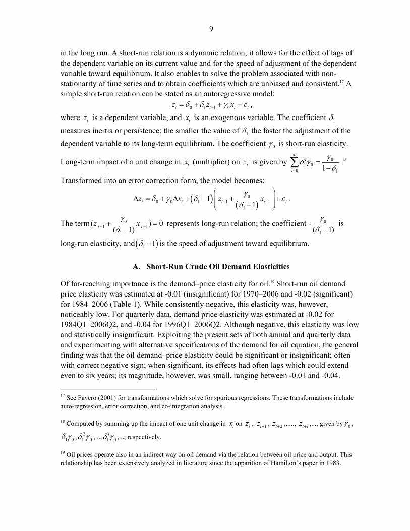
in the long run. A short-run relation is a dynamic relation; it allows for the effect of lags of the dependent variable on its current value and for the speed of adjustment of the dependent variable toward equilibrium. It also enables to solve the problem associated with non-stationarity of time series and to obtain coefficients which are unbiased and consistent.17 A simple short-run relation can be stated as an autoregressive model:
0 1 1 0t t t tz z xδ δ γ ε−= + + + , where tz is a dependent variable, and tx is an exogenous variable. The coefficient 1δ measures inertia or persistence; the smaller the value of 1δ the faster the adjustment of the dependent variable to its long-term equilibrium. The coefficient 0γ is short-run elasticity.
Long-term impact of a unit change in tx (multiplier) on tz is given by 01 0
0 11i
i
γδ γδ
∞
=
=−∑ .18
Transformed into an error correction form, the model becomes:
( ) ( )0
0 0 1 1 11
11t t t t tz x z xγδ γ δ ε
δ− −
⎛ ⎞Δ = + Δ + − + +⎜ ⎟⎜ ⎟−⎝ ⎠
.
The term 01 1
1
( ) 0( 1)t tz xγδ− −+ =−
represents long-run relation; the coefficient - 0
1( 1)γ
δ − is
long-run elasticity, and ( )1 1δ − is the speed of adjustment toward equilibrium.
A. Short-Run Crude Oil Demand Elasticities
Of far-reaching importance is the demand–price elasticity for oil.19 Short-run oil demand price elasticity was estimated at -0.01 (insignificant) for 1970–2006 and -0.02 (significant) for 1984–2006 (Table 1). While consistently negative, this elasticity was, however, noticeably low. For quarterly data, demand price elasticity was estimated at -0.02 for 1984Q1–2006Q2, and -0.04 for 1996Q1–2006Q2. Although negative, this elasticity was low and statistically insignificant. Exploiting the present sets of both annual and quarterly data and experimenting with alternative specifications of the demand for oil equation, the general finding was that the oil demand–price elasticity could be significant or insignificant; often with correct negative sign; when significant, its effects had often lags which could extend even to six years; its magnitude, however, was small, ranging between -0.01 and -0.04. 17 See Favero (2001) for transformations which solve for spurious regressions. These transformations include auto-regression, error correction, and co-integration analysis.
18 Computed by summing up the impact of one unit change in tx on tz , 1tz + , 2tz + ,....., t iz + ,..., given by 0γ ,
1 0δ γ , 21 0δ γ ,..., 1 0
iδ γ ,..., respectively.
19 Oil prices operate also in an indirect way on oil demand via the relation between oil price and output. This relationship has been extensively analyzed in literature since the apparition of Hamilton’s paper in 1983.

10
Table 1. Crude Oil and Natural Gas: Short-Term Demand and Supply Elasticities Variable 1970–2006 1984–2006 84Q1–06Q2 96Q1–06Q2
Coeff. T-Stat. Coeff. T-Stat. Coeff. T-Stat. Coeff. T-Stat.Crude oil demand
Lagged dependent 0.54 5.08 0.04 0.32 0.63 7.43 0.54 5.23 Crude oil price -0.01 -1.28 -0.02 -2.17 -0.02 -1.30 -0.04 -1.15
World GDP 0.12 3.12 0.44 6.48 0.20 3.98 0.19 2.13 Interest rate -0.006 -2.55 0.003 1.70 0.001 1.29 -0.002 -1.11
NEER -0.023 -0.19 -0.17 -3.12 -0.03 -2.29 -0.07 -2.17 2R 0.96 0.99 0.97 0.96
DW 1.93 1.78 1.84 1.86 Crude oil supply
Lagged dependent 0.72 8.32 0.72 6.78 0.79 14.23 0.71 8.95 Crude oil price 0.02 1.29 0.02 1.76 0.01 2.67 0.02 2.45
Oil reserves 0.14 3.16 0.21 2.49 0.14 3.39 0.11 1.74 2R 0.94 0.98 0.97 0.95
DW 1.53 1.91 1.86 1.67 Natural gas demand
Lagged dependent 0.79 10.4 0.33 3.09 0.65 8.01 0.25 2.80 Natural gas price -0.04 -3.29 -0.01 -1.02 -0.11 -2.70 -0.04 -1.63 Crude oil price 0.01 2.75 -0.02 -2.00 0.01 2.37 0.02 2.41
World GDP 0.11 1.84 0.41 5.72 0.26 4.25 0.48 4.23 Interest rate -0.003 -2.14 0.001 0.71 0.001 1.21 -0.005 -2.55
NEER 0.10 1.18 -0.16 -2.21 -0.05 -3.53 -0.04 -1.51 2R 0.99 0.99 0.99 0.98
DW 2.37 2.58 1.96 1.54 Natural gas supply
Lagged dependent 0.84 8.72 0.75 7.10 0.79 16.2 0.75 9.56 Natural gas price 0.05 3.53 0.05 3.73 0.04 3.55 0.03 1.51 Crude oil price -0.05 -3.83 -0.03 -1.86 -0.01 -1.95 -0.002 -0.26 Gas reserves 0.05 0.76 0.08 1.02 0.12 3.58 0.13 2.52
2R 0.99 0.99 0.99 0.97 DW 2.05 2.28 2.05 1.77
Further, the significance and size of this parameter changed with model specification and parsimony. As illustrated by the following two demand relationships for 1970–2006, a parsimonious oil demand equation tended to yield significant demand price elasticity: LQ = 0.769*LQ(-1) - 0.0275*LP(-1) + 0.103*LY + 0.62; 2R = 0.96; DW=1.9. (t=8.43) (t=-3.64) (t=3.25) (t=2.33) LQ = 0.733*LQ(-1)-0.315*LQ(-2)-0.0388*LP(-6)+0.231*LY+1.56 ; 2R = 0.97; DW=1.82. (t=5.30) (t=-2.42) (t=-5.14) (t=5.60) (t=5.10)

11
In the first regression, demand–price elasticity was estimated at -0.0275, significant at lag 1; in the second regression, this elasticity was estimated at -0.0388, significant at lag 6, implying that a strong oil shock, such as the first oil shock, could have a significant effect on oil demand for several periods. Furthermore, in order to address multicollinearity in lagged prices, a polynomial distributed lag in oil prices, with 6 lags and polynomial degree equal to 2, was estimated for 1970–2006 yielding the regression below. While price elasticities were consistently negative, they tended to be very small and statistically insignificant, except at lag 5. The sum of these elasticities, computed at -0.05776, was significant, indicating a significant cumulative effect of oil prices on oil demand. LQ = 0.532*LQ(-1) -0.006*LP-0.006*LP(-1)-0.0065*LP(-2)-0.0074*LP(-3)-0.0087*LP(-4) (t=4.09) (t=-0.57) (t=-1.53) (t=-1.30) (t=-1.11) (t=-1.53) -0.0102*LP(-5) - 0.01256*LP(-6) + 0.196*LY + 1.297; 2R = 0.97; DW=1.44; (t=-3.08) (t=-1.55) (t=4.21) (t=3.52) Sum of lags = -0.05776 (t=-4.62). These results are crucial for understanding world oil markets. World demand for oil seemed to have very little response to oil price changes in the short-run. Despite changing data frequency and sample periods, regression analysis tended to yield consistently very low short-run demand price elasticities, with often insignificant contemporaneous effect, and significance achieved only with lag. Extreme demand price inelasticity can be easily interpreted economically. First, crude oil is a basic commodity and thus shares the properties of basic commodities whose consumption cannot be reduced without impairing dramatically consumers’ welfare. Second, short-run demand for oil products is determined by fixed capital, including refining capacity, machinery, transport fleet, appliances, and by the state of arts; it cannot change instantaneously with changes in prices.20 Substitution, or energy-saving, effects are limited in the short-run; they become important only in the long-run. This price-inelasticity is a source of high price volatility, which could drive prices to record peaks or troughs, and has major implications. At the level of consumers, oil price increases will increase proportionally the budget share on oil spending, and will reduce the budget share for non-oil commodities; consequently, non-oil demand will be depressed; the consumer’s new commodity bundle will include approximately the same quantity of oil, however, fewer non-oil commodities. At the level of taxation, governments can levy high taxes on oil products without impairing the tax-yield. At the level of international trade, oil importing countries have limited room for cutting oil imports, and therefore consent to larger imports bills. At the level of oil producers, this inelasticity may confer market power to oil producers that may allow them to influence oil prices.
20 For instance, a water desalination plant, or a power generation station, has to meet an average load of demand, and does not cut or increase supply because of short-run fluctuations in fuel prices.

12
The income effect was consistently significant and relatively high. The income elasticity was estimated at 0.12 for 1970–2006, and 0.44 for 1984–2006. For quarterly data, the income elasticity was estimated at 0.20 for 1984Q1–2006Q2, and 0.19 for 1996Q1–2006Q2. Based on the present data sets and running several regressions, the general finding was that the income elasticity was significant; however, it was sensitive to the sample period and frequency and to the specification of the oil demand relationship. A parsimonious demand model tended to yield higher, however, always less than unity, income elasticity. The size and significance of the income elasticity imply that world economic growth exerts a significant positive effect on world demand for oil. The high value of the short-run income elasticity explains business cycles characterizing oil markets. International economic recession explains lax oil demand and oil price downturn cycles. Hence, recessionary episodes during 1980–1982 and 1997–1998 might have contributed to observed downturn cycles in oil prices in these two time intervals. In contrast, an expanding world economy explains tight oil markets conditions and upturns in oil prices; such was the case during 2000-2006. Although significant, income elasticity was less than unity. Subsequently, world oil demand would fluctuate less in magnitude compared to the case of an income elasticity higher than unity. Contrary to price-elasticity, income elasticity exhibited considerable instability. It seemed to have increased from 0.12 in 1970–2006 to 0.44 in 1984–2006. As income elasticity rises, oil markets become more sensitive to business cycles. This paper was particularly interested in studying short-run implications of monetary policy on oil markets. For this purpose, world demand for oil included LIBOR and the U.S. effective nominal exchange rate; both variables exhibited wide movements and are indicators of monetary policy stance as well as the stability of major reserve currencies. Omission tests indicated that these two variables together had a significant impact on oil demand. For annual data, LIBOR had a significant and negative effect, with a lag of 2 periods, on world demand for crude oil. The semi-elasticity was significant and was of the order of -0.006 for 1970–2006. For 1984–2006, the interest rate semi-elasticity, estimated at 0.003, had an unexpected sign and was statistically insignificant. For 1984Q1–2006Q2, LIBOR coefficient, estimated at 0.001, had also an unexpected sign and was insignificant. For 1996Q1–2006Q2, the interest rate semi-elasticity, estimated at -0.002, was negative and insignificant. Based on the two data sets at hand, the general finding for the interest rate semi–elasticity was that this parameter could be significant or insignificant with expected (negative) or unexpected (positive) sign; its significance depended essentially on the sample period, namely whether the sample period corresponded to a period of active monetary policy, and on the parsimony of specification of the demand relationship, as illustrated by the following two regressions, which included episodes of highly active monetary policies.
13
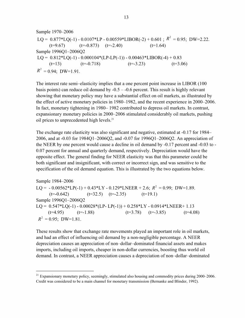
Sample 1970–2006 LQ = 0.877*LQ(-1) - 0.0107*LP - 0.00559*LIBOR(-2) + 0.601 ; 2R = 0.95; DW=2.22. (t=9.67) (t=-0.873) (t=-2.40) (t=1.64) Sample 1996Q1–2006Q2 LQ = 0.812*LQ(-1) - 0.000104*(LP-LP(-1)) - 0.00463*LIBOR(-4) + 0.83 (t=13) (t=-0.718) (t=-3.23) (t=3.06)
2R = 0.94; DW=1.91. The interest rate semi–elasticity implies that a one percent point increase in LIBOR (100 basis points) can reduce oil demand by -0.5 – -0.6 percent. This result is highly relevant showing that monetary policy may have a substantial effect on oil markets, as illustrated by the effect of active monetary policies in 1980–1982, and the recent experience in 2000–2006. In fact, monetary tightening in 1980– 1982 contributed to depress oil markets. In contrast, expansionary monetary policies in 2000–2006 stimulated considerably oil markets, pushing oil prices to unprecedented high levels.21 The exchange rate elasticity was also significant and negative, estimated at -0.17 for 1984–2006, and at -0.03 for 1984Q1–2006Q2, and -0.07 for 1996Q1–2006Q2. An appreciation of the NEER by one percent would cause a decline in oil demand by -0.17 percent and -0.03 to -0.07 percent for annual and quarterly demand, respectively. Depreciation would have the opposite effect. The general finding for NEER elasticity was that this parameter could be both significant and insignificant, with correct or incorrect sign, and was sensitive to the specification of the oil demand equation. This is illustrated by the two equations below. Sample 1984–2006 LQ = - 0.00562*LP(-1) + 0.43*LY - 0.129*LNEER + 2.6; 2R = 0.99; DW=1.89. (t=-0.642) (t=32.5) (t=-2.35) (t=19.1) Sample 1996Q1–2006Q2 LQ = 0.547*LQ(-1) - 0.00028*(LP- LP(-1)) + 0.258*LY - 0.0914*LNEER+ 1.13 (t=4.95) (t=-1.88) (t=3.78) (t=-3.85) (t=4.08) 2R = 0.95; DW=1.81. These results show that exchange rate movements played an important role in oil markets, and had an effect of influencing oil demand by a non-negligible percentage. A NEER depreciation causes an appreciation of non–dollar–dominated financial assets and makes imports, including oil imports, cheaper in non-dollar currencies, boosting thus world oil demand. In contrast, a NEER appreciation causes a depreciation of non–dollar–dominated
21 Expansionary monetary policy, seemingly, stimulated also housing and commodity prices during 2000–2006. Credit was considered to be a main channel for monetary transmission (Bernanke and Blinder, 1992).
14
financial assets and makes imports, including oil imports, more expensive in non-dollar currencies, and depresses in turn world oil demand. The coefficient of the lagged dependent variable describes a first order difference equation in the dependent variable, giving the speed of adjustment toward full equilibrium, following a random shock or a change in any of the exogenous variables.22 For annual data, world demand for crude oil showed considerable stickiness during1970 –2006, which was captured by the significant coefficient of the lagged demand, estimated at 0.54. However, this inertia seemed to have disappeared for annual data in 1984–2006. Annual world demand seemed to be close to its long-run path during 1984–2006. For quarterly data, inertia remained significant and high. Estimates of the lagged dependent variable coefficient were 0.63 for 1984Q1–2006Q2, and 0.54 for 1996Q1–2006Q2. Quarterly world demand was, therefore, away from its long-run equilibrium, and may take two to three quarters to return to equilibrium following a shock.
B. Short-Run Natural Gas Demand Elasticities
Natural gas demand was affected negatively by its own-price. Own–price elasticity was estimated at -0.04 (significant) for 1970–2006, and -0.01 (insignificant) for 1984–2006. For quarterly data, demand–price elasticity was estimated at -0.11 (significant) and -0.04 (insignificant), for 1984Q1–2006Q2 and 1996Q1–2006Q2, respectively. Hence, similar to oil demand, short-run gas demand may have only a small response to changes in own price. The same explanation applies; namely, gas consumption is determined by fixed physical capital which cannot be changed in the short-run in response to changes in prices. However, in a longer-run period, consumers do respond to persistent trends in prices and adapt their gas consumption accordingly. Cross-price elasticity with oil price is an important parameter which enables to assess the degree of interaction between oil and gas markets. While there was no noticeable natural gas shock, as gas is less tradable than oil, major oil shocks had a strong impact on gas markets, affecting both quantities and prices. The first oil shock displaced large oil demand toward gas wherever substitution was feasible in residential, commercial, and industrial uses. This is easily perceived from the increasing trend in the natural gas to crude oil output and price
22 The effect of a random shock is given by the impulse response function. Indeed, if a vector auto-regression
(VAR) system is written as: 1
L
t i t i ti
y y ε−=
= Φ +∑ , ( )'t tE ε ε = Σ , under invertibility condition, the VAR has a
moving average representation defined as: 0
t i t ii
y ε∞
−=
= Ψ∑ . The impulse response function consists of
computing the iΨ .

15
ratios (Figure 1). For instance, associated natural gas was no longer flared and was recuperated; natural gas became an important feedstock in petrochemicals; gas to liquids technologies were being developed with a view to reducing the cost for producing petroleum products from gas. In transportation, natural gas use was also increasing. Estimates for 1970–2006 showed a significant positive effect of higher oil prices on gas demand. Cross-oil price
80
100
120
140
160
180
70 72 74 76 78 80 82 84 86 88 90 92 94 96 98 00 02 04 06
0
50
100
150
200
250
70 72 74 76 78 80 82 84 86 88 90 92 94 96 98 00 02 04 06
Figure 1a: Ratio of Natural Gas to Crude Oil Output, 1970-2006.
Figure 1b. Ratio of Natural Gas to Crude Oil Price, 1970-2006.
elasticity, estimated at 0.01, was, however, low, indicating that changes in oil price had a significant, but small effect on natural gas demand in the short-run. In contrast, estimate for 1984–2006 showed a negative cross-oil price elasticity, -0.02. This negative effect could illustrate an asymmetric response of gas demand to oil prices; in particular, large oil price downturns would not cause reverse substitution from gas toward oil. Estimates for 1984Q1–2006Q2 and 1996Q1–2006Q2, seemed to indicate positive and significant cross-price elasticity, ranging between 0.01 and 0.02, indicating that higher oil prices tended to increase demand for gas. The most plausible cross-oil price elasticity would be a positive one. Such result would corroborate the significant substitution that has taken place since the first oil shock between gas and oil in many uses. Similar to oil demand, gas demand had significant income elasticity. For 1970–2006, short-run income elasticity was estimated at 0.11. However, for 1984–2006, it was estimated at 0.41, indicating a prominent role for world income in driving world demand for gas. This result is indicative of major structural changes in world demand for gas and large substitution of natural gas in many energy uses. Thus, as gas use kept increasing in many sectors of world economy, gas demand became more sensitive to world economic activity. Income elasticity

16
was estimated at 0.26 for 1984Q1–2006Q2, and seemed to have risen to 0.48 for 1996Q1–2006Q2. With gas use spreading to many sectors of the economy, world economic activity seemed to have become more gas intensive. Hence, gas will have an increasing role in influencing world activity. Effects of monetary policy on gas markets have also been examined. Omission test indicated that LIBOR and NEER acted significantly on demand for gas. The interest rate coefficient was highly sensitive to demand specification. A parsimonious model would yield a highly significant interest rate coefficient. For 1970–2006, interest rate semi-elasticity was estimated at -0.003 (significant). Thus, an increase in interest rates by 100 basis points could decelerate world demand for gas by -0.3 percent. For 1996Q1–2006Q2, interest rate semi-elasticity, at -0.005, was significant. Clearly, an active monetary policy would have a significant effect on demand for gas. Exchange rate may also have a significant effect on the demand for gas. The NEER elasticity was estimated at -0.16 for 1984–2006 (significant). For quarterly data, the NEER elasticity was estimated at -0.05 (significant) for 1984Q1–2006Q2, and -0.04 (insignificant) for 1996Q1–2006Q2. Thus, currency instability could affect world demand for gas, mostly via wealth effect stemming from changes in real value of financial assets. Econometric analysis showed that both interest and exchange rates’ elasticities could be significant in more parsimonious specifications and through changing the sample period. For instance, for 1998Q1–2006Q2, as shown by the regression below, interest rate semi-elasticity was estimated at -0.004 (significant), and NEER elasticity was estimated at -0.06 (significant), indicating that active monetary policy had significantly stimulated demand for gas during this sample period. Sample 1998Q1–2006Q2 LG = 0.327*LG(-1) - 0.0034*(LPG-LPG(-1)) + 0.0359*LP(-2) + 0.276*LY - (t=2.41) (t=-0.50) (t=3.78) (t=2.04) 0.00468*LIBOR(-2) – 0.060*LNEER + 3.21; 2R = 0.98; DW=2.23. (t=-3.59) (t=-2.71) (t=5.06) Gas demand was exhibiting high stickiness in 1970–2006, with the coefficient of the lagged dependent variable estimated at 0.79. Thus, the 1973 and 1979 oil shocks displaced demand for gas far away from long-run equilibrium. As structural adjustment in demand was taking place over time, inertia diminished. The auto-regression coefficient was estimated at 0.33 (significant) for 1984–2006, indicating much less displacement of gas demand from long-run equilibrium and faster return to this equilibrium following shocks. For quarterly data, lagged dependent variable coefficient was estimated at 0.65 (significant) for 1984Q1–2006Q2; demand for gas showed much less inertia in 1996Q1–2006Q2, with the lagged dependent variable coefficient dropping to 0.25 (significant), indicating substantial structural change in demand for gas, and faster return of this demand to long-run equilibrium following changes in driving variables or random shocks.
17
Comparing oil and gas demand relationships, it can be noted that these two relationships exhibited close structural patterns. Both showed correct-signed and significant demand price elasticity; however, this elasticity was extremely low. Both demands were driven by the level of economic activity, and were experiencing rising income elasticities. With regard to monetary policy, both variables were significantly responsive to changes in interest and exchange rates. Thus, monetary policy can affect considerably both oil and gas markets, and therefore, cause significant changes in energy prices. Regarding the autoregressive coefficient (i.e. the inertia effect), gas demand seemed to have higher stickiness. While both demands underwent substantial structural adjustment, it seemed that oil demand became more flexible, and faster to converge toward steady-state equilibrium than gas demand.
C. Short-Run Crude Oil Supply Elasticities
The ratio of gas to oil output has an increasing time trend, and may have a close relationship to the price ratio (Figure 1). Indeed, a simple regression relating the two ratios gives:
L(Q/G )= 0.34*L(P/PG) - 2.62; 2R = 0.67; DW=0.92. (t=8.35) (t=-29.07) The significance of the relationship between oil and gas output and price ratios would call for exploring the effects of gas variables on oil variables. However, to keep the model recursive, only the impact of oil on the gas sector is studied. For 1970–2006 and 1984–2006, oil supply–price elasticity was estimated at 0.02 (insignificant). For 1984Q1–2006Q2, oil supply price elasticity was estimated at 0.01 (significant). For 1996Q1–2006Q2, price elasticity was estimated at 0.02 (significant), indicating that oil supply was showing a small response to upturn movements in oil prices during 1999-2006. Thus, there is considerable short-run price inelasticity in oil supply. Oil production seemed to be determined by prevailing capacity for production, proven reserves, storage, and refining, and also by existing contracts and prevailing quotas for OPEC members, with small influence of oil prices. As supply was price insensitive, shocks to oil demand would lead to wide changes in oil prices, as witnessed during business cycles. Besides oil price, oil supply was also related to oil proven reserves. As increases in proven reserves stemmed partly from investment in the oil sector, conveying thus indirect information on capital spending and potential capacity, oil reserves seemed to be a pertinent variable for explaining oil supply (Fisher (1964), Erickson and Spann (1971), Eyssell (1978), and Dhal and Duggan (1998))23. Oil reserves elasticity was estimated at 0.14 (significant) for 1970–2006; it rose to 0.21 (significant) for 1984–2006, indicating more intensive pumping.
23 In Fisher (1964), Erickson and Spann (1971), Dhal and Duggan (1998), oil production is related to reserves,
often in the form of a depletion equation: 0t
tQ e ORSVα−= . According to these authors, reserves are related to oil price and drilling activities.

18
For quarterly data, reserves elasticity was estimated at 0.14 (significant) for 1984Q1–2006Q2, and 0.11 (insignificant) for 1996Q1–2006Q2. These elasticities indicated that an increase in reserves would lead to a non-negligible increase in oil supply. Considerable rigidity characterized oil supply, as shown by high and significant coefficient of lagged supply, indicating that oil supply, once disturbed by a shock, had a slow adjustment speed toward equilibrium. For 1970–2006, the autoregressive coefficient was estimated at 0.72. For 1984–2006, oil supply continued to show high inertia. Similar inertia characterized oil supply during 1984Q1–2006Q2, and 1996Q1–2006Q2, with autoregressive coefficients estimated at 0.79 and 0.71, respectively.
D. Short-Run Natural Gas Supply Elasticities
The large magnitude of some historical oil shocks seemed to have influenced substantially and positively gas supply. To the extent that oil price shocks contributed to a general appreciation of energy prices, including gas prices, they might have contributed to make investment in the gas industry more appealing than before the shocks, causing therefore an expansion of gas supply. Indeed, the under-supply of natural gas in the fifties and sixties and gas shortage in the seventies could be attributed to low oil prices prior to 1973 oil shock, which discouraged exploratory activities for gas. Following this shock, and consequent appreciation of gas prices, a large effort world-wide was made for exploring and exploiting gas resources. Figure 1 shows a steady increase in the ratio of gas to oil supply, with natural gas gaining a higher share in the hydrocarbons industry. The price of natural gas has appreciated significantly in relation to crude oil price during 1970–2006. As shown above, a regression of the supply ratio on the price ratio yielded a significant elasticity, indicating that gas suppliers were responding to the appreciation of gas prices in terms of oil prices.
Gas supply was positively influenced by own price. Supply price elasticity was estimated at 0.05 (significant) for 1970–2006 and 1984–2006. For quarterly data, it was estimated at 0.04 (significant) for 1984Q1–2006Q2, and 0.03 (insignificant) for 1996Q1–2006Q2. Cross-oil price elasticity was estimated at -0.05 (significant) for 1970–2006, and -0.03 (significant) for 1984–2006. For quarterly data, it was estimated at -0.01 (significant) for 1984Q1–2006Q2, and -0.002 (insignificant) for 1996Q1–2006Q2. Hence, gas–oil price ratio was a main determinant (with correct sign) of gas supply. An appreciation of gas price in relation to oil price would lead to higher gas supply; and vice-versa, depreciation of the price ratio would lead to lower gas supply. Gas reserves coefficient was estimated at 0.05 (insignificant) for 1970–2006, and 0.08 (insignificant) for 1984–2006. For quarterly data, it was estimated at 0.12 (significant) for 1984Q1–2006Q2, and 0.13 (significant) for 1996Q1–2006Q2. The gas reserves elasticity was concomitant with the structural change in the gas industry. Prior to the first oil shock, gas was in large part an associated product with oil as the gas industry was in a lull state. Following the 1973 oil shock and reviving interest in natural gas, more gas fields were discovered and put into exploitation, explaining thus the rising elasticity of gas reserves.
19
Regarding the dynamic adjustment of gas supply, the autoregressive coefficient seemed to indicate slow speed of adjustment. This coefficient was estimated at 0.84 for 1970–2006, and 0.75 for 1984–2006. For quarterly data, the auto-regression coefficient was at 0.79 for 1984Q1–2006Q2, and 0.75 for 1996Q1–2006Q2. Thus, when disturbed, gas supply adjusted slowly to long-run equilibrium. This could be explained by technological considerations, such as more investment was undertaken in gas fields, more gas production was coming on line, and more distribution network or processing facilities were being installed. As the gas sector kept expanding, convergence toward equilibrium remained slow. Oil and gas supply equations displayed similar characteristics. They were influenced positively by own price. They were also positively influenced by own reserves. Interaction between the two equations was taken to be one way interaction; cross-oil price elasticity was shown to be small and negative.
IV. SIMULATION OF THE MODEL AND MULTIPLIER ANALYSIS
To serve as a forecast tool a SEM has to fit closely the actual data. It would be interesting to see whether the model could produce the observed sharp fluctuations in oil and gas prices. The simulation exercise was undertaken for annual data 1970─2006, and for quarterly data 1984Q1─2006Q2. Both sets of data included episodes of oil shocks, large fluctuations in quantities and prices, and therefore provide a rich data set for evaluating the in-sample performance of the model. If performance is acceptable, meaning that the root of mean squared error is small, the annual model could be applied for annual forecast, and the quarterly model for quarterly forecast.
A. Simulation of the Annual Model: Sample 1970─2006
The structural form of the annual model can be stated as follows: Crude Oil Demand LQ = 0.542*LQ(-1) - 0.0111*LP(-4) + 0.123*LY - 0.00561*LIBOR(-2) (SE) (0.107) (0.00868) (0.0395) (0.0022) - 0.0231*LNEER + 1.52; sigma = 0.0241663 (0.118) (0.421) Inverse Crude Oil Supply LP = 0.713*LP(-1) + 1.16*LQ - 0.521*LORSV(-2) + 0.324*DUMO - 0.454 (SE) (0.0625) (0.672) (0.313) (0.0506) (1.26) sigma = 0.167612 Natural Gas Demand LG = 0.792*LG(-1) - 0.0396*(LPG(-1) -LPG(-2)) + 0.0143*LP(-4)+ 0.11*LY (SE) (0.0762) (0.012) (0.0052) (0.0596) - 0.00304*LIBOR(-2) + 0.0961*LNEER + 0.932; sigma = 0.0144985 (0.00142) (0.0813) (0.421) Inverse Natural Gas Supply

20
LPG = 0.9*LPG(-1) + 0.514*LG + 0.0378*LP - 0.18*LGRSV + 0.26*DUMG- 2.6 (SE) (0.0654) (0.435) (0.0757) (0.327) (0.0301) (1.84) sigma = 0.0864828. The model tracked closely the data (Figure 2). The residuals were white noise. The respective values for the standard error of the regression residuals (sigma) were 0.02 for oil demand, 0.168 for inverse oil supply, 0.014 for gas demand, and 0.086 for inverse gas supply. Hence, oil and gas outputs have close fit with actual data. However, due to their high volatility, oil and gas prices tended to exhibit higher standard error for the residuals. The implication for forecasting would be to allow for larger errors for price forecast. Assessing the in-sample forecast, the model seemed to replicate fluctuations in oil and gas prices; however, large fluctuations might be underestimated by the model. For instance, gas prices were excessively volatile during 2000–2006, rising suddenly by 68 percent in 2000, falling by 26 percent in 2002, and then rising sharply by 69 percent in 2003, 37 percent in 2005, and falling by 9 percent in 2006. These wide gyrations in gas prices caused the model’s in-sample forecast to become less precise. With regard to oil prices, in-sample forecast during 2000–2006 was rather satisfactory due to persistence in rising trend during this period. In light of the in-sample forecast performance, it seems that wider error margin should be allowed for prices compared to quantities in future short-term forecast.
B. Simulation of the Quarterly Model: Sample 1984Q1─2006Q2
The structural form of the quarterly model can be stated as follows: Crude Oil Demand LQ = 0.628*LQ(-1) - 0.0152*(LP-LP(-1)) + 0.204*LY + 0.00124*LIBOR(-2) (SE) (0.0866) (0.0131) (0.0518) (0.00109) - 0.034*LNEER + 0.774; sigma = 0.0151522 (0.0159) (0.183) Inverse Crude Oil Supply LP = 0.941*LP(-1) + 0.529*LQ(-2) - 0.229*LORSV + 0.181*DUMO - 0.448 (SE) (0.0286) (0.301) (0.239) (0.0141) (0.665) sigma = 0.0847762. Natural Gas Demand LG = 0.649*LG(-1) - 0.107*(LPG-LPG(-1)) + 0.0132*LP + 0.257*LYW (SE) (0.0818) (0.0393) (0.0051) (0.0614) + 0.000989*LIBOR(-2) - 0.0524*LNEER + 1.24; sigma = 0.0142549 (0.000812) (0.0149) (0.278) Inverse Natural Gas Supply LPG = 0.58*LPG(-1) + 0.687*LG(-1) + 0.138*LP - 0.311*LGRSV - 3.07 (SE) (0.0768) (0.257) (0.0359) (0.175) (0.836) sigma = 0.0745424

21
The quarterly model fitted closely the actual data (Figure 3). The residuals were white noise. The respective values for the standard error of the regression residuals were 0.015 for oil demand, 0.085 for inverse oil supply, 0.014 for gas demand, and 0.075 for inverse gas supply. Because of their low volatility, oil and gas outputs had a close fit with actual data. However, due to their high volatility, oil and gas prices tended to exhibit higher standard error for the residuals. Nonetheless, the model was replicating the trend for oil and gas prices during 1984Q1─2006Q2. The performance of the model during 2000Q1─2006Q2 could be considered as satisfactory as the residuals were tightly contained in a small error margin.
Figure 2. Annual Simulation of the Oil and Natural Gas Model, 1970–2006.
1980 1990 2000
4.14.24.34.4 LQ Fitted
1980 1990 2000
0
2r:LQ (scaled)
1980 1990 2000
3
4LP Fitted
1980 1990 2000-1012 r:LP (scaled)
1980 1990 20007.257.507.758.00
LG Fitted
1980 1990 2000
-1012 r:LG (scaled)
1980 1990 2000
4567
LPG Fitted
1980 1990 2000
0
2r:LPG (scaled)

22
Figure 3. Quarterly Simulation of the Oil and Natural Gas Model, 1984Q1–2006Q2.
1985 1990 1995 2000 2005
4.14.24.34.4
LQ Fitted
1985 1990 1995 2000 2005
-2
0
2 r:LQ (scaled)
1985 1990 1995 2000 2005
3
4lp Fitted
1985 1990 1995 2000 2005
0.0
2.5
5.0r:lp (scaled)
1985 1990 1995 2000 2005
6.2
6.4
6.6lg Fitted
1985 1990 1995 2000 2005
0
2
4r:lg (scaled)
1985 1990 1995 2000 20050.250.500.751.00 lpg Fitted
1985 1990 1995 2000 2005
-2.5
0.0
2.5 r:lpg (scaled)
C. Multiplier Analysis
Model multipliers are key parameters, which compute the effect of a change in exogenous variables on endogenous variables; they may be derived directly from the model’s long-run reduced form, assuming lagged endogenous variables to be at steady–state equilibrium. If stylized values are assigned to multipliers, one can evaluate rapidly the impact of changes in exogenous variables on oil and gas outputs and prices. Given the noted instability of structural parameters over sample periods and frequencies, it is important to examine the multipliers over the four sample periods considered for the model (Table 2).

23
Table 2. Multiplier Analysis Variable
Sample Period
World Income
Interest Rate
Exchange Rate
Oil Reserves
Gas Reserves
1970–2006 0.246 -0.011 -0.046 0.040 0.000 1984–2006 0.330 0.002 -0.129 0.128 0.000 84Q1–06Q2 0.548 0.003 -0.091 0.000 0.000
Crude Oil Output
96Q1–06Q2 0.462 -0.004 -0.169 -0.008 0.000 1970–2006 0.991 -0.045 -0.185 -1.654 0.000 1984–2006 6.853 0.043 -2.690 -6.940 0.000 84Q1–06Q2 4.921 0.030 -0.820 -3.882 0.000
Crude Oil Price
96Q1–06Q2 3.251 -0.031 -1.192 -0.487 0.000 1970–2006 0.593 -0.018 0.448 -0.114 0.000 1984–2006 0.428 0.001 -0.163 0.182 0.000 84Q1–06Q2 0.917 0.004 -0.180 -0.146 0.000
Natural Gas Output
96Q1–06Q2 0.714 -0.007 -0.094 -0.013 0.000 1970–2006 3.433 -0.108 2.239 -1.211 -1.809 1984–2006 7.674 0.045 -3.005 -6.882 -0.423 84Q1–06Q2 3.122 0.016 -0.565 -1.519 -0.739
Natural Gas Price 96Q1–06Q2 1.957 -0.019 -0.398 -0.115 -0.039
The multiplier for world income shows that a one percent increase in income could easily induce 0.5 percent increase in oil demand, and 0.9 percent increase in gas demand. Consequently, this may cause an increase in oil prices by 7 percent and in gas prices by 8 percent. The multiplier for interest and exchange rates were generally negative, indicating that expansionary monetary policy leading to lower interest rates and depreciating NEER might stimulate oil and gas markets. Inversely, tight monetary policy leading to higher interest rates and appreciating NEER might depress oil and gas markets. The multiplier for oil reserves tended to stimulate oil output and depress oil prices; its effect on gas output was ambiguous; however, it seemed to depress gas prices. The multiplier for gas reserves does not impact oil markets due to the recursive nature of the model. Nonetheless, it tended to stimulate gas output, and depress gas prices.
V. STRUCTURAL VECTOR AUTO-REGRESSION ANALYSIS
After having analyzed the model multipliers, it would be worthy also studying the impact of random shocks, and learn more about the historic dynamics of oil and gas markets. Such an analysis is undertaken by viewing the SEM as a near─vector autoregressive (VAR) model

24
comprising four variables: oil output, oil price, gas output, and gas price.24 Four shocks are identified: an oil demand shock operating through the oil demand function, an oil supply shock operating through the oil supply function, a gas demand shock operating via the gas demand function, and a gas supply shock operating through the gas supply function. Impulse responses of VAR to shocks are shown in Figure 4 and 5. The first row in Figure 4 and 5 describes the impact of an oil demand shock, the second describes the impact of an oil supply shock, the third describes the impact of a gas demand shock, and the fourth describes the impact of a gas supply shock on successively oil output, oil price, gas output, and gas price. A demand shock increases demand for oil. At the same time, it contributes to a gradual increase in oil prices, and gas output and price. This seems to be the experience during 2000─2006 when a demand shock caused an increase in oil demand, and at the same a progressive increase in oil price, gas output, and gas price. In contrast, a supply shock seems to act abruptly, causing sharp increase in oil prices, depressing in turn oil demand. It causes, however, an increase in gas output and prices, via essentially a displacement of oil demand toward gas. A gas demand shock increases demand for gas as well as gas prices. A gas supply shock increases gas prices, and depresses at the same time gas demand. It operates along the same pattern as an oil supply shock. Because of assumed recursiveness, shocks from the gas sector are not transmitted to the oil sector. As mentioned earlier, recursiveness is assumed only to simplify modeling; reverse relationship would be worth analyzing, as developments in the gas sector do affect the oil sector.
VI. CONCLUSIONS
Recent instability in oil and gas prices, coupled with expansionary monetary policy and re-emergence of inflationary expectations, motivated building a model for analyzing oil and gas markets, with an explicit role for monetary policy. Using annual data for 1970─2006 and quarterly data for 1984Q1─2006Q2, far-reaching findings regarding structural parameters were established. In this respect, short-term oil demand price elasticity turned out to be small, ranging between -0.01 and -0.04, often contemporaneously insignificant and significant only with lag, showing a highly price inelastic word demand for oil. Short-term oil supply-price elasticity turned out also to be small. Similar demand and supply elasticties were obtained for the gas sector. As implication of these findings, any small imbalance in hydrocarbons demand or supply could lead to large changes in respective prices. In examining oil-gas linkage, cross-oil price elasticity was shown to be small, positive in the gas demand equation, and negative in the gas supply equation. Oil and gas demands were driven by world economic activity. Income elasticity has always been significant and could range between
24A Vector Autoregressive (VAR) model including oil prices, interest rates, and exchange rates (Krichene, 2005 and 2006) showed a two-way causality between interest rates and oil prices, and that the recent oil shock was mainly caused by expansionary monetary policy in major industrial countries.

25
Figure 4. Annual Structural VAR: Impulse Responses
0 20 40
0.0
0.5
1.0 LQ (LQ eqn)
0 20 400.00.51.01.5 LP (LQ eqn)
0 20 40
0.000
0.025
0.050 LG (LQ eqn)
0 20 40
0.1
0.2
0.3 LPG (LQ eqn)
0 20 40
-0.010-0.0050.000 LQ (LP eqn)
0 20 40
0.0
0.5
1.0 LP (LP eqn)
0 20 40
0.00
0.01
0.02 LG (LP eqn)
0 20 400.0250.0500.0750.100 LPG (LP eqn)
0 20 40
0.0
0.1 LQ (LG eqn)
0 20 40
0.0
0.1 LP (LG eqn)
0 20 40
0.5
1.0 LG (LG eqn)
0 20 40
0.5
1.0
1.5 LPG (LG eqn)
0 20 40
0.0
0.1 LQ (LPG eqn)
0 20 40
0.0
0.1 LP (LPG eqn)
0 20 40
-0.02
0.00LG (LPG eqn)
0 20 40
0.5
1.0 LPG (LPG eqn)
Figure 5. Quarterly Structural VAR: Impulse Responses
0 50
0.5
1.0 LQ (LQ eqn)
0 50
0.5
1.0LP (LQ eqn)
0 500.000.010.020.03 LG (LQ eqn)
0 50
0.10.20.30.4 LPG (LQ eqn)
0 50-0.015-0.010-0.0050.000 LQ (LP eqn)
0 50
0.5
1.0 LP (LP eqn)
0 50
0.00
0.01
0.02 LG (LP eqn)
0 50
0.1
0.2
0.3 LPG (LP eqn)
0 50
0.0
0.1 LQ (LG eqn)
0 50
0.0
0.1 LP (LG eqn)
0 50
0.5
1.0 LG (LG eqn)
0 50
0.250.500.75 LPG (LG eqn)
0 50
0.0
0.1 LQ (LPG eqn)
0 50
0.0
0.1 LP (LPG eqn)
0 50
-0.10
-0.05
0.00 LG (LPG eqn)
0 50
0.5
1.0 LPG (LPG eqn)
0.11 and 0.48. It has been systematically less than unity. As implication of this finding, changes in the rate of world economic growth would cause significant changes in demand for oil and gas and subsequently could cause large upturns or downturns in oil and gas prices. The paper was particularly interested in the role of monetary policy in oil and gas markets. It showed that interest rate, given by LIBOR, had a significant and negative semi-elasticity, implying that an active monetary policy would influence, with some delay, significantly oil and gas demand. Similarly, the U.S. nominal effective exchange rate, used as a measure for

26
exchange rates stability, showed that exchange rate movements had significant and negative effect on oil and gas demands. A depreciation of the U.S. dollar exchange rate would contribute to stimulate world hydrocarbon demand, and vice-versa. As implication of these findings, highly active monetary policy would have a significant effect on oil and gas markets. In the same vein, stable monetary conditions would contribute to stable oil and gas markets. These findings suggest that monetary policy has to include in the monetary policy rule impact of monetary instruments (e.g., interest rate, money base) on oil and gas prices.
Historical simulation showed that the model fitted closely data; its dynamics were able to retrace turning points in actual quantity and price data. In-sample quantity forecast has very small error margins. Price forecast, however, deteriorated when there were wild fluctuations in prices. If applied as a forecasting tool, the model has to assume wider error for prices. The paper analyzed the model’s multipliers and impulse responses to demand and supply shocks. In this regard, an oil demand shock has a typical response consisting of an increase in demand for oil and gas, and a gradual increase in prices which tapers off progressively. An oil supply shock has a typical response consisting of a price increase, depressed oil demand, and increased gas output and prices.
As any econometric model, deficiencies cannot be ruled out; and further modeling improvement would be desirable by addressing the exogeneity of income, and interest and exchange rates, bringing in expected rate of inflation, and using real interest rates as argument in the demand equations. Nonetheless, the SEM, being a structural model and involving key macroeconomic variables, has many potential applications for industry analysts and policymakers. It could be used as a forecasting tool for oil and gas quantities and prices under hypothetical scenarios for exogenous variables. It could also simulate the impact of random shocks to demand and supply of oil and gas via impulse responses.

27
Estimated Regressions
Annual Data Crude Oil Demand, Sample 1970─2006 LQ = 0.542*LQ(-1) - 0.0111*LP(-4) + 0.123*LY - 0.00561*LIBOR(-2) (SE) (0.107) (0.00868) (0.0395) (0.0022) - 0.0231*LNEER + 1.52; sigma = 0.0241663. (0.118) (0.421) Crude Oil Demand, Sample 1984─2006 LQ = 0.044*LQ(-1) - 0.0177*LP(-2) + 0.437*LY + 0.00273*LIBOR(-2) (SE) (0.141) (0.00817) (0.0673) (0.0016) - 0.171*LNEER + 2.49; sigma = 0.0104882. (0.0549) (0.354) Crude Oil Supply, Sample 1970─2006 LQ = 0.717*LQ(-1) + 0.0207*(LP- LP(-1))+ 0.137*LORSV(-2) + 0.27; sigma = 0.061. (SE) (0.0861) (0.016) (0.0433) (0.179) Crude Oil Supply, Sample 1984─2006 LQ = 0.7225*LQ(-1) + 0.02088*LP(-1) + 0.2113*LORSV - 0.3438; sigma = 0.02882. (SE) (0.107) (0.0118) (0.0848) (0.223) Natural Gas Demand, Sample 1970─2006 LG = 0.792*LG(-1) - 0.0396*(LPG(-1)-LPG(-2)) + 0.0143*LP(-4) (SE) (0.0762) (0.012) (0.0052) + 0.11*LY - 0.00304*LIBOR(-2) + 0.0961*LNEER + 0.932; sigma = 0.0144985 (0.0596) (0.00142) (0.0813) (0.421) Natural Gas Demand, Sample 1984─2006 LG = 0.327*LG(-1) - 0.0108*(LPG(-1) -LPG(-2)) - 0.0177*LP(-2) (SE) (0.106) (0.0107) (0.00882) + 0.409*LY + 0.00119*LIBOR(-2) - 0.157*LNEER + 3.75; sigma = 0.0097947 (0.0715) (0.00168) (0.0713) (0.616) Natural Gas Supply, Sample 1970─2006 LG = 0.839*LG(-1) + 0.0485*LPG - 0.0459*LP(-1) + 0.0511*LGRSV+ 0.879 (SE) (0.0963) (0.0137) (0.0119) (0.0674) (0.416) sigma = 0.01182. Natural Gas Supply, Sample 1984─2006 LG = 0.754*LG(-1) + 0.0463*LPG - 0.0259*LP(-1) + 0.0844*LGRSV + 1.33 (SE) (0.106) (0.0124) (0.0139) (0.0824) (0.416) sigma = 0.0102. Quarterly Data Crude Oil Demand, Sample 1984Q1─2006Q2 LQ = 0.632*LQ(-1) - 0.0165*(LP-LP(-1)) + 0.204*LY + 0.00137*LIBOR(-2) (SE) (0.0851) (0.0127) (0.0511) (0.00106)

28
- 0.0356*LNEER + 0.766; sigma = 0.0150062. (0.0156) (0.179) Crude Oil Demand, Sample 1996Q1─2006Q2 LQ = 0.539*LQ(-1) - 0.0373*LP + 0.0443*LP(-1) + 0.193*LY - 0.00191*LIBOR(-4) (SE) (0.103) (0.0324) (0.0301) (0.0906) (0.00173) - 0.0674*LNEER + 1.35; sigma = 0.0102828 (0.031) (0.275) Crude Oil Supply, Sample 1984Q1─2006Q2 LQ = 0.793*LQ(-1) + 0.014*LP(-1) + 0.139*LORSV(-2) - 0.132; sigma = 0.032. (SE) (0.056) (0.005) (0.041) (0.104) Crude Oil Supply, Sample 1996Q1─2006Q2 LQ = 0.714*LQ(-1) + 0.017*LP(-1) + 0.114*LORSV(-2) + 0.366; sigma = 0.058. (SE) (0.079) (0.007) (0.066) (0.356) Natural Gas Demand, Sample 1984Q1─2006Q2 LG = 0.647*LG(-1) - 0.113*(LPG - LPG(-1))+ 0.0117*LP + 0.258*LY + (SE) (0.0808) (0.0147) (0.00492) (0.0607) 0.00096*LIBOR(-2) - 0.0521*LNEER + 1.25; sigma = 0.0144115 (0.000793) (0.0417) (0.275) Natural Gas Demand, Sample 1996Q1─2006Q2 LG = 0.249*LG(-1) - 0.0432*(LPG -LPG(-1) )+ 0.019*LP(-2) (SE) (0.135) (0.0265) (0.0079) + 0.479*LY - 0.00471*LIBOR(-4) - 0.0441*LNEER + 2.73 ; sigma = 0.010683 (0.113) (0.00185) (0.0293) (0.488) Natural Gas Supply, Sample 1984Q1─2006Q2 LG = 0.79*LG(-1) + 0.0427*LPG(-1) - 0.0112*LP(-4) + 0.122*LGRSV + 0.75 (SE) (0.0486) (0.012) (0.00575) (0.0341) (0.156) sigma = 0.011. Natural Gas Supply, Sample 1996Q1─2006Q2 LG = 0.752*LG(-1) + 0.0281*LPG(-1) - 0.00226*LP(-4) + 0.133*LGRSV+ 0.918 (SE) (0.0787) (0.0186) (0.00854) (0.0528) (0.373) sigma = 0.031.
29
References
Amano, R. A. and S. van Norden, 1998, “Exchange Rates and Oil Prices,” Review of International Economics, Vol. 6 Issue 4 Page 683.
Balestra, P., and M. Nerlove, 1966, “Pooling Cross Section and Time Series Data in the
Estimation of a Dynamic Model: The Demand for Natural Gas,” Econometrica, Vol. 34, pp. 585-612.
Bernanke, B.S., and A.S. Blinder, 1992, “The Federal Funds Rate and the Channels of
Monetary Transmissions,” American Economic Review, Vol. 82, No. 4, pp. 901─21. Bernanke, B.S., M. Gertler, and M. Watson, 1997, “Systematic Monetary Policy and the
Effects of Oil Shocks,” Brookings Papers on Economic Activity, Vol. 1997, No. 1, pp. 91─157.
Dhal, C., and T. E. Duggan, 1998, “Survey of Price Elasticities from Economic Exploration
Models of US Oil and Gas Supply,” Journal Energy Finance and Development, Vol. 3, No. 2, pp. 129–169.
Erickson, E.W., and R.M. Spann, 1971, “Supply Response in a Regulated Industry: The Case
of Natural Gas,” The Bell Journal of Economics and Management Science, Vol. 2, No. 1, pp. 94─121.
Eyssell, J. H., 1978, “The Supply Response of Crude Petroleum – New and Optimistic
Results,” Business Economics 1393, pp. 338-346. Favero, C. A., 2001, Applied Macroeconometrics, Oxford University Press.
Fisher, F.M., 1964, Supply Costs in the United States Petroleum Industry, John Hopkins, University Press.
Gately, D., and H.G. Huntington, 2002, “The Asymmetric Effects of Changes in Price and
Income on Energy and Oil Demand,” The Energy Journal, Vol. 23, No. 1, pp. 19─55. Hamilton, J.D., 1983, “Oil and the Macroeconomy since World War II,” Journal of Political
Economy, 91, pp. 228─48. Hamilton, J.D., 2003, “What Is an Oil Shock,” Journal of Econometrics, 113, pp. 363─98. Hamilton, J.D., and A.M. Herrera, 2004, “Oil Shocks and Aggregate Macroeconomic
Behavior: The Role of the Monetary Policy,” Journal of Money, Credit, and Banking, Vol. 36, No. 2, pp. 265─86.
30
Jones, D.W., P.N. Leiby, and I.K. Paik, 2004, “Oil Price Shocks and the Macroeconomy:
What Have We Learned Since 1996?,” The Energy Journal, Vol. 25, No. 2, pp. 1─32. Krichene, N., 2002, “World Crude Oil and natural Gas: A Demand and Supply Model,”
Energy Economics, Vol. 24, pp. . Krichene, N., 2005, “A Simultaneous Equations Model for World Crude Oil and Natural Gas
Markets,” IMF Working paper WP/05/32. Krichene, N., 2006, “World Crude Oil Markets: Monetary Policy and the Recent Oil Shock,”
IMF Working Paper WP/06/62. McCallum, B. and W. Nelson, 2000, “Performance of Operational Policy Rules in an
Estimated Semi-Classical Structural Model,” in Monetary Policy Rules, ed. by John Taylor (Chicago: University of Chicago Press).
McFadden, D., and M. Fuss, Eds., 1977, Production Economics: A Dual Approach.
Amsterdam: North-Holland Publishing Co. Muth, J. F., 1961, "Rational Expectations and the Theory of Price Movements,"
Econometrica, Vol. 29 no. 3, pp. 313─335. Pesaran, M.H., R.P. Smith, and T. Akiyama, 1998, Energy Demand in Asian Developing
Economies, (New York: Oxford University Press/World Bank). Pindyck, R. S., 1979, The Structure of World Energy Demand (Cambridge, Massachusetts:
MIT Press). Williamson, J., 1983, The Open Economy and the World Economy; Basic Books, New York. Working, E. J., 1927, “What Do Statistical Demand Curves Show?” Quarterly Journal of
Economics; Vol. 41, pp. 212-235.