An NS2 TCP Evaluation Tool:

Installation Guide and Tutorial (V0.2)

Gang Wang, Yong Xia David HarrisonNEC Laboratories China BitTorrent

{wanggang, xiayong}@research.nec.com.cn dave@bittorrent.com

November 24, 2008

Abstract

A TCP performance evaluation tool for the network simulator NS2 has been developed. Thisdocument describes how to install and use this tool.

[Release History]

• V0.1 released on 2007/04/29.

• V0.2 released on 2008/11/24. It adds the scenarios advised by TMRG.

1

Contents

1 Introduction 4

2 Installation 42.1 Install the Components One-by-One . . . . . . . . . . . . . . . . . . . . . . . . . . . 42.2 Install the All-in-one Patch . . . . . . . . . . . . . . . . . . . . . . . . . . . . . . . . 6

3 Tool Components 73.1 Network Topologies . . . . . . . . . . . . . . . . . . . . . . . . . . . . . . . . . . . . . 7

3.1.1 A Single-Bottleneck Dumb-Bell Topology . . . . . . . . . . . . . . . . . . . . 73.1.2 A Multiple-Bottleneck Parking-Lot Topology . . . . . . . . . . . . . . . . . . 73.1.3 A Simple Network Topology . . . . . . . . . . . . . . . . . . . . . . . . . . . . 7

3.2 Traffic Models . . . . . . . . . . . . . . . . . . . . . . . . . . . . . . . . . . . . . . . . 93.2.1 Long-lived FTP Traffic . . . . . . . . . . . . . . . . . . . . . . . . . . . . . . . 93.2.2 Short-lived Web Traffic . . . . . . . . . . . . . . . . . . . . . . . . . . . . . . 93.2.3 Streaming Video Traffic . . . . . . . . . . . . . . . . . . . . . . . . . . . . . . 93.2.4 Interactive Voice Traffic . . . . . . . . . . . . . . . . . . . . . . . . . . . . . . 93.2.5 Tmix . . . . . . . . . . . . . . . . . . . . . . . . . . . . . . . . . . . . . . . . 9

3.3 Performance Metrics . . . . . . . . . . . . . . . . . . . . . . . . . . . . . . . . . . . . 103.3.1 Throughput, Delay, Jitter and Loss Rate . . . . . . . . . . . . . . . . . . . . 103.3.2 Response Times and Oscillations . . . . . . . . . . . . . . . . . . . . . . . . . 113.3.3 Fairness and Convergence . . . . . . . . . . . . . . . . . . . . . . . . . . . . . 113.3.4 Robustness in Challenging Environments . . . . . . . . . . . . . . . . . . . . 11

3.4 Simulation Results . . . . . . . . . . . . . . . . . . . . . . . . . . . . . . . . . . . . . 11

4 Usage Details 114.1 Example 1: A Simple Simulation . . . . . . . . . . . . . . . . . . . . . . . . . . . . . 124.2 Example 2: The TCP Variants Used in the Simulation . . . . . . . . . . . . . . . . . 124.3 Example 3: Scenario Configuration . . . . . . . . . . . . . . . . . . . . . . . . . . . . 13

4.3.1 Parameter Settings . . . . . . . . . . . . . . . . . . . . . . . . . . . . . . . . . 134.3.2 Tool Configuration . . . . . . . . . . . . . . . . . . . . . . . . . . . . . . . . . 13

4.4 Example 4: Multiple Output Formats . . . . . . . . . . . . . . . . . . . . . . . . . . 144.4.1 Text Format . . . . . . . . . . . . . . . . . . . . . . . . . . . . . . . . . . . . 144.4.2 HTML Format . . . . . . . . . . . . . . . . . . . . . . . . . . . . . . . . . . . 144.4.3 EPS Format . . . . . . . . . . . . . . . . . . . . . . . . . . . . . . . . . . . . . 15

4.5 Example 5: A Convergence Time Test . . . . . . . . . . . . . . . . . . . . . . . . . . 164.6 Example 6: A Comparison of the TCP Variants’ Performance . . . . . . . . . . . . . 17

5 TMRG TCP Evaluation Suite 195.1 A: Basic Scenario . . . . . . . . . . . . . . . . . . . . . . . . . . . . . . . . . . . . . . 19

5.1.1 Typical settings . . . . . . . . . . . . . . . . . . . . . . . . . . . . . . . . . . . 195.1.2 Collected parameters . . . . . . . . . . . . . . . . . . . . . . . . . . . . . . . . 205.1.3 Outputs . . . . . . . . . . . . . . . . . . . . . . . . . . . . . . . . . . . . . . . 21

5.2 Other scenarios in the PFLDnet paper . . . . . . . . . . . . . . . . . . . . . . . . . . 215.2.1 B: Delay/throughput tradeoff as function of queue size . . . . . . . . . . . . . 215.2.2 C: Convergence times: completion time of one flow . . . . . . . . . . . . . . . 22

2

5.2.3 D: Transients: release of bandwidth, arrival of many flows . . . . . . . . . . . 235.2.4 E: Impact on standard TCP traffic . . . . . . . . . . . . . . . . . . . . . . . . 235.2.5 F: Intra-protocol and inter-RTT fairness . . . . . . . . . . . . . . . . . . . . . 245.2.6 G: Multiple bottlenecks . . . . . . . . . . . . . . . . . . . . . . . . . . . . . . 24

5.3 Known Problems . . . . . . . . . . . . . . . . . . . . . . . . . . . . . . . . . . . . . . 25

6 Changed files list 25

7 Acknowledgements 27

3

1 Introduction

Researchers frequently use the network simulator NS2 to evaluate the performance of their protocolsin the early stage of design. One particular area of recent intest is the congestion control protocols(a.k.a., TCP alternatives) for high-speed, long-delay networks. There is significant overlap among(but lack of a community-agreed set of) the topologies, traffic, and metrics used by many researchersin the evaluation of TCP alternatives: effort could be saved by starting research from an existingframework. As such, we developed a TCP performance evaluation tool. This tool includes severaltypical topologies and traffic models; it measures some of the most important metrics commonlyused in TCP evaluation; and it can automatically generate simulation statistics and graphs readyfor inclusion in latex and html documents. The tool is very easy to use and contains an extendableopen-source framework.

This tool can be used not only for high-speed TCP protocols, but for other proposed changes tocongestion control mechanisms as well, such as ECN added to SYN/ACK packets, changes to makesmall transfers more robust, changes in RTO estimation, and proposals to distinguish between lossdue to congestion or corruption, etc.

This simulation tool does not attempt to be a final one. Instead, it intends to serve as a startingpoint. We invite community members to contribute to the project by helping to extend this tooltoward a widely-accepted, well-defined set of NS2 TCP evaluation benchmarks.

Below we describe how to install and use this tool for TCP performance evaluation.

2 Installation

This tool builds upon a set of previous work. There are two ways to install the tool: #1) installall the required components one by one, or #2) install an “all-in-one” patch that includes all theneeded components. We recommend the approach #2, but will first describe the approach #1 forclarity purpose.

2.1 Install the Components One-by-One

First you need to install NS2. Our tool has been tested with ns-2.29, ns-2.30, and ns-2.31. But werecommend the most recent version. Suppose you install the ns-allinone-2.31 package (available athttp://www.isi.edu/nsnam/ns/ns-build.html) under the directory $HOME/ns-allinone-2.31.

Second, you need to install the RPI NS2 Graphing and Statistics package from http://www.ecse.rpi.edu/∼harrisod/graph.html, which provides a set of classes for generating commonly usedgraghs and gathering important statistics.

Third, you need the PackMime-HTTP Web Traffic Generator from http://dirt.cs.unc.edu/packmime/. This package is implemented in NS2 by the researchers at UNC-Chapel Hill based ona model developed at the Internet Traffic Research group of Bell Labs. It generates synthetic webtraffic in NS2 based on the recent Internet traffic traces.

Fourth, to test the high-speed TCP protocols you have to install them, e.g.,

4

* HTCP, designed by R. Shorten and D. Leith, downloadable from http://www.hamilton.ie/net/research.htm#software (with STCP implementation included);

* BIC/CUBIC, designed by L. Xu and I. Rhee, downloadable from http://www.csc.ncsu.edu/faculty/rhee/export/bitcp/bitcp-ns/bitcp-ns.htm and http://www.csc.ncsu.edu/faculty/rhee/export/bitcp/cubic-script/script.htm;

* FAST, designed by S. Low, C. Jin, and D. Wei, implemented in NS2 by T. Cui and L.Andrew, downloadable from http://www.cubinlab.ee.mu.oz.au/ns2fasttcp;

* VCP, designed by Y. Xia, L. Subramanian, I. Stoica, and S. Kalyanaraman, downloadablefrom http://networks.ecse.rpi.edu/∼xiay/vcp.html;

The ns-allinone-2.31 distribution includes other TCP protocols like Reno, SACK, HSTCP (S.Floyd), and XCP (D. Katabi and M. Handley).You can also add whichever protocols according toyour need.

In V0.2 release, the tool uses tmix as one of the traffic generators. The download page is,* M.C. Weigle, P. Adurthi, F. Hernandez-Campos, K. Jeffay, and F.D. Smith, Tmix: A Tool

for Generating Realistic Application Workloads in ns-2, ACM SIGCOMM CCR, July 2006, Vol 36,No 3, pp. 67-76. http://www.cs.odu.edu/˜mweigle/TrafGen/Releases;

Finally, install our tool from http://sourceforge.net/projects/tcpeval. Just unpack thepackage to the NS2 root directory $HOME/ns-allinone-2.31.

> cd $HOME/ns-allinone-2.31> tar zxvf tcpeval-0.2.tar.gz

This creates a directory called eval under $HOME/ns-allinone-2.31. The eval directory con-tains all the scripts and documents of our tool. To use this tool, an environment variable TCPEVALmust be defined. You can define it in the file $HOME/.bash profile to avoid doing this repeatedly.

> export TCPEVAL=$HOME/ns-allinone-2.31/eval

In V0.2 release, we use tmix-pp provided by Dr. M. Weigle to analyze tmix trace. Users arerequired make it able to run.

> chmod +x $TCPEVAL/tmix-tool/pp

Now you can try an example simulation provided in the tool.

> cd $TCPEVAL/ex # directory for examples> ns test_dumb_bell.tcl # a dumb_bell topology simulation

5

2.2 Install the All-in-one Patch

To ease the installation process, we also provide a patch file for the latest ns-allinone package(version 2.31 as of the date this document was written). This patch contains all the componentsdescribed above.

First, go to http://www.isi.edu/nsnam/ns/ns-build.html, download the ns-allinone-2.31package. Again, suppose you install the package under the directory $HOME/ns-allinone-2.31.

Second, go to http://sourceforge.net/projects/tcpeval, download the patch file ns-allinone-2.31.tcpeval-0.2.patch.gz, and then install the patch. The TCP evaluation tool will appear inthe directory $HOME/ns-allinone-2.31/eval.

> cd $HOME # note it is $HOME directory> gunzip ns-allinone-2.31.tcpeval-0.2.patch.gz> patch -p0 < ns-allinone-2.31.tcpeval-0.2.patch

Now rebuild the NS2 package. To do that, first, you need to configure the environment settings.In the file $HOME/.bash profile, set NS to the directory containing the NS2 package, NSVER to theNS2 version, and TCPEVAL to the directory of the TCP evaluation tool scripts.

> export NS=$HOME/ns-allinone-2.31/ns-2.31> export NSVER=2.31> export TCPEVAL=$HOME/ns-allinone-2.31/eval

Then configure the RPI Graphing and Statistics package and rebuild NS2.

> ns $HOME/ns-allinone-2.31/ns-2.31/tcl/rpi/configure.tcl> cd $HOME/ns-allinone-2.31/ns-2.31> ./configure> make depend> make

In V0.2 release, we use tmix-pp provided by Dr. M. Weigle to analyze tmix trace. Users arerequired make it able to run.

> chmod +x $TCPEVAL/tmix-tool/pp

Now you can try an example simulation provided in the tool.

> cd $TCPEVAL/ex # directory for examples> ns test_dumb_bell.tcl # a dumb_bell topology simulation

6

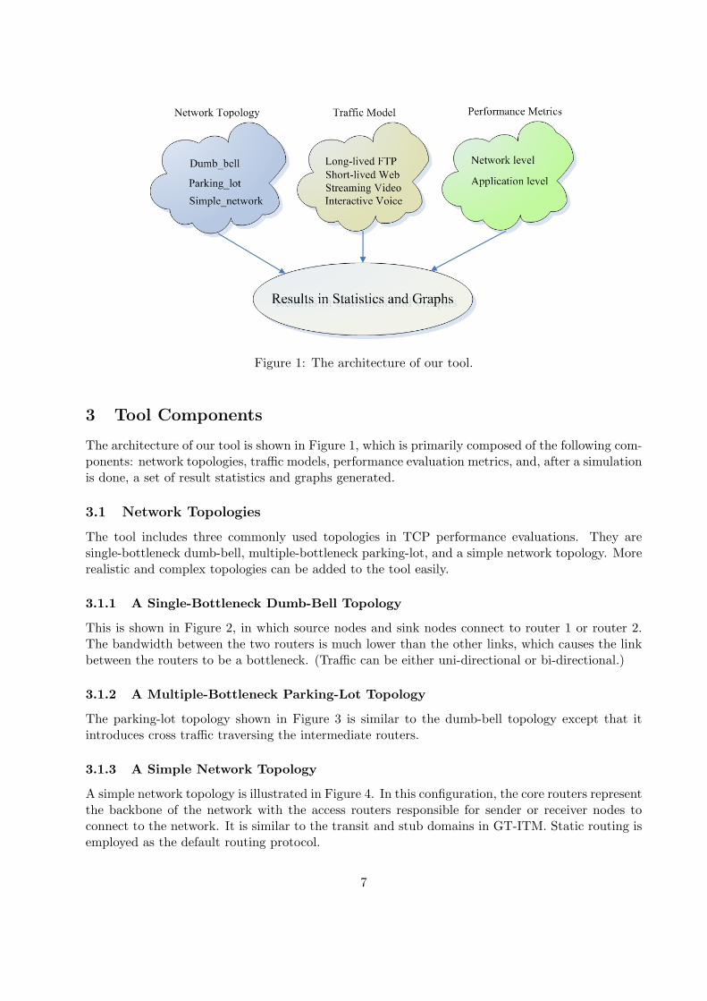
Figure 1: The architecture of our tool.

3 Tool Components

The architecture of our tool is shown in Figure 1, which is primarily composed of the following com-ponents: network topologies, traffic models, performance evaluation metrics, and, after a simulationis done, a set of result statistics and graphs generated.

3.1 Network Topologies

The tool includes three commonly used topologies in TCP performance evaluations. They aresingle-bottleneck dumb-bell, multiple-bottleneck parking-lot, and a simple network topology. Morerealistic and complex topologies can be added to the tool easily.

3.1.1 A Single-Bottleneck Dumb-Bell Topology

This is shown in Figure 2, in which source nodes and sink nodes connect to router 1 or router 2.The bandwidth between the two routers is much lower than the other links, which causes the linkbetween the routers to be a bottleneck. (Traffic can be either uni-directional or bi-directional.)

3.1.2 A Multiple-Bottleneck Parking-Lot Topology

The parking-lot topology shown in Figure 3 is similar to the dumb-bell topology except that itintroduces cross traffic traversing the intermediate routers.

3.1.3 A Simple Network Topology

A simple network topology is illustrated in Figure 4. In this configuration, the core routers representthe backbone of the network with the access routers responsible for sender or receiver nodes toconnect to the network. It is similar to the transit and stub domains in GT-ITM. Static routing isemployed as the default routing protocol.

7

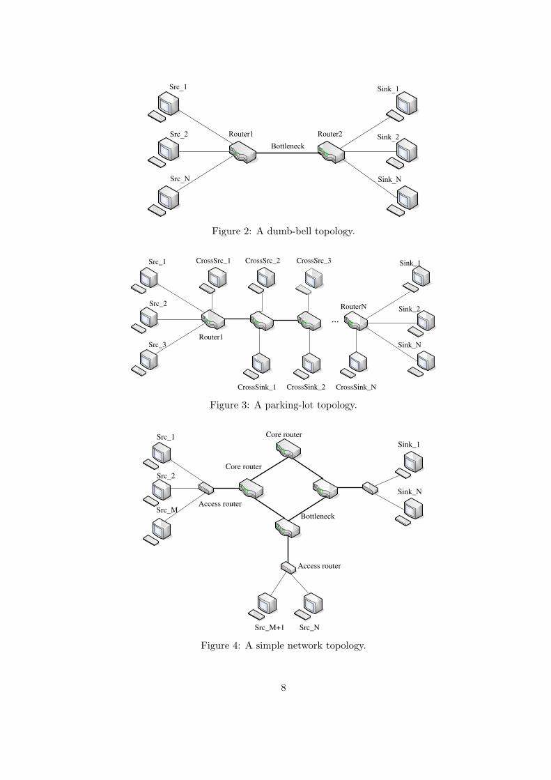
Figure 2: A dumb-bell topology.

Router1

Src_1 Sink_1CrossSrc_2

CrossSink_2

RouterN

CrossSrc_1

CrossSink_1

Src_2

Src_3

CrossSrc_3

CrossSink_N

Sink_2

Sink_N

...

Figure 3: A parking-lot topology.

Core router

Core router

Bottleneck

Src_1

Src_M+1

Access router

Access router

Src_2

Src_M

Sink_1

Sink_N

Src_N

Figure 4: A simple network topology.

8

3.2 Traffic Models

The tool attempts to apply the typical traffic settings. The applications involved include fourcommon traffic types.

3.2.1 Long-lived FTP Traffic

FTP traffic uses infinite, non-stop file transmission, which begins at a random time and runs onthe top of TCP. Implementation details and choice of TCP variants are decided by users, which isnot in the scope of this tool.

3.2.2 Short-lived Web Traffic

The web traffic module employs the PackMime HTTP traffic generator, which is available in therecent NS2 releases.

3.2.3 Streaming Video Traffic

Streaming traffic is modeled using CBR traffic over UDP. Both sending rate and packet size aresettable.

3.2.4 Interactive Voice Traffic

There are currently two synthetic voice traffic generation methods available in this tool. One isbased on CBR-like streaming traffic. The other is generated according to a two-state ON/OFFmodel, in which ON and OFF states are exponentially distributed. The mean ON period is 1.0sec, and the mean OFF duration is 1.35 sec. These values are set in accordance with ITU-Trecommendations, but are changeable if needed.

The voice packet size is 200 bytes, including the 160 bytes data packet (codec G.711, 64 kbpsrate and 20 ms duration), 20 byte IP header, 8 byte UDP header, and 12 byte RTP header. Theseparameters can be changed by using other voice/audio codecs.

3.2.5 Tmix

Although we have included the above traffic generation methods, but today, few networks carryonly one or two applications or such classes. The links usually carry various application packets.On the other hand, some applications, such as P2P, have no appropriate models that could be usedin the simulation and evaluation. To generate such scenarios, tmix 1, a tool for generating realisticTCP application workloads is included. It takes the trace taken from a network link of interest,and generates the connection vectors which are used for emulating the behavior of the applications.

Currently, tmix only works for FULLTCP scheme. One way TCP implementation is expectedlater.

1M. Weigle, P. Adurthi, F. Hernandez-Campos, K. Jeffay and F. Smith, Tmix: a tool for generating realistic TCPapplication workloads in ns-2, ACM SIGCOMM CCR, Volume 36 , Issue 3, pp. 65 - 76, July 2006

9

3.3 Performance Metrics

A comprehensive list of the metrics for TCP performance evaluation is described in the TMRGRFC “Metrics for the Evaluation of Congestion Control Mechanisms” by S. Floyd. In the first step,this tool tries to implement some commonly used metrics described there. Here we follow the RFCand classify the metrics into network metrics and application metrics. They are listed as follows.

3.3.1 Throughput, Delay, Jitter and Loss Rate

• Throughput

For network metrics, we collect bottleneck link utilization as the aggregate link throughput.

Throughput is sometimes different from goodput, because goodput consists solely of usefultransmitted traffic, where throughput may also include retransmitted traffic. But users caremore about the useful bits the network can provide. So the tool collects application levelend-to-end goodput no matter what the transport protocol is employed.

For long-lived FTP traffic, it measures the transmitted traffic during some intervals in bitsper second.

For short-lived web traffic, the PackMime HTTP model collects request/response goodputand response time to measure web traffic performance.

Voice and video traffic are different from above. Their performance is affected by packetdelay, delay jitter and packet loss rate as well as goodput. So their goodput is measured intransmitted packet rate excluding lost packets and delayed packets in excess of a predefineddelay threshold.

• Delay

We use bottleneck queue size as an indication of queuing delay in bottlenecks. Besides meanand max/min queue size statistics, we also use percentile queue size to indicate the queuelength during most of the time.

FTP traffic is not affected much by packet transmission delay.

For web traffic, we report on the response time, defined as the duration between the client’ssending out requests and receiving the response from the server.

For streaming and interactive traffic, packet delay is a one-way measurement, as defined bythe duration between sending and receiving at the end nodes.

• Jitter

Delay jitter is quite important for delay sensitive traffic, such as voice and video. Large jitterrequires much more buffer size at the receiver side and may cause high loss rates in strictdelay requirements. We employ standard packet delay deviation to show jitter for interactiveand streaming traffic.

• Loss Rate

To obtain network statistics, we measure the bottleneck queue loss rate.

We do not collect loss rates for FTP and web traffic because they are less affected by thismetric.

10

For interactive and streaming traffic, high packet loss rates result in the failure of the receiverto decode the packet. In this tool, they are measured during specified intervals. The receivedpacket is considered lost if its delay is beyond a predefined threshold.

3.3.2 Response Times and Oscillations

One of the key concerns in the design of congestion control mechanisms has been the response timeto sudden network changes. On the one hand, the mechanism should respond rapidly to changesin the network environment. On the other hand, it has to make sure changes are not too severe toensure the stability of the network. This tool is designed so the response time and fluctuations canbe easily observed using a series of figures it generates, if the simulation scenarios we use includevariable bandwidth, round trip delay, various traffic start times and other parameters.

3.3.3 Fairness and Convergence

In this tool, the fairness measurement uses Jain’s fairness index to measure the fair bandwidthshare of end-to-end FTP flows that traverse the same route.

Convergence times are the time elapsed between multiple flows from an unfair share of linkbandwidth to a fair state. They are quite important for environments with high-bandwidth, long-delay flows. This tool includes scenarios to test the convergence performance.

3.3.4 Robustness in Challenging Environments

A static link packet error model has been introduced in the tool to investigate TCP performancein challenging environments. Link failure, routing changes and other diagnostic markers can easilybe tested by changing the tool’s parameters.

3.4 Simulation Results

The tool includes the RPI graphing package to automatically generate the above-discussed perfor-mance metrics. At the end of a simulation, it also automatically generates a series of user-definedstatistics (e.g. bottleneck average utilization, bottleneck 90-percentile queue length, average per-flow goodput, etc.) and graphs (like bottleneck utilization and queue length variation over time,per-flow throughput over time, etc). It can create latex and html files in order to present thesimulation results in a paper or webpage form. All the simulation-generated data is stored in atemporary directory for later use.

4 Usage Details

Before using this tool, you should have some experience about NS2. All the examples shown beloware those commonly used in TCP performance evaluation.

The main body of this tool includes three files: create topology.tcl, create traffic.tcl,and create graph.tcl in the $HOME/ns-allinone-2.31/eval/tcl directory. As their file namesindicate, create topology.tcl implements the three common network topologies discussed inSection 3.1, create traffic.tcl defines the traffic model parameters in the simulation (see Section3.2), and crate graph.tcl generates simulation statistics (see Section 3.3.1) and plots graphs atthe end of simulations.

11

Three example scripts are given in the $HOME/ns-allinone-2.31/eval/ex directory. Theyare test dumb bell.tcl, test parking lot.tcl and test network 1.tcl for the above-discussedtopologies. Their parameters definitions are in def dumb bell.tcl, def parking lot.tcl, anddef network 1.tcl, respectively.

Here, we take the dumb bell topology simulation as an example; simulations for other topologiesare the similar.

4.1 Example 1: A Simple Simulation

Users are recommended to run the example scripts as a starting point. For example,

> cd $TCPEVAL/ex> ns test_dumb_bell.tcl

It will run the dumb-bell topology simulation with default parameters defined indef dumb bell.tcl. The results can be reviewed by opening /tmp/index100.html.

The output format will be explained in the following Section 4.4. If one wants to write his ownexamples, the following code should be incorporated into his tcl script.

source $TCPEVAL/tcl/create_topology.tclsource $TCPEVAL/tcl/create_traffic.tclsource $TCPEVAL/tcl/create_graph.tcl

4.2 Example 2: The TCP Variants Used in the Simulation

Before evaluating a TCP variant, one must make sure that the protocol exists in his NS2 simulator.Or, it will give an error message “No such TCP installed in ns2”. Reno, SACK, HSTCP, and XCPexist in the NS 2.31 distribution. Other TCP variants should be put into NS2 before they canbe used. After that, one needs to set their configuration parameters used in the simulation. Forexample, if one wants to evaluate the performance of VCP, firstly he needs to download the VCPcode from the following link and install it according to its manual.

http://networks.ecse.rpi.edu/~xiay/vcp.html

Then the configuration parameters for VCP need to be set in the procedure get tcp params ofcreate topology.tcl.

if { $scheme == "VCP" } {set SRC TCP/Reno/VcpSrc # For VCP source and sink.set SINK VcpSinkset QUEUE DropTail2/VcpQueue # Bottleneck Queue....

}

To simplify the above process, the all-in-one patch has included six other TCP variants’ im-plementations and settings: STCP, HTCP, BIC, CUBIC, FAST, and VCP. For the details, pleaserefer to Section 2.1 for their implementation and typical settings.

12

4.3 Example 3: Scenario Configuration

When start to simulate a scenario, firstly, one needs to set the parameters used in the simulation,and then, send them to the tool. Here, we take the dumb-bell topology as an example.

4.3.1 Parameter Settings

The parameter setting in def dumb bell.tcl includes three parts: topology setting, traffic setting,and simulation statistics and graph setting. The topology setting defines the specific topologyparameters. For dumb-bell, it sets the bottleneck bandwidth, round trip time, propagation delay,and packet error rate in the bottleneck link. The traffic setting defines the traffic parameters usedin the simulation, such as the number of FTP traffic, what high-speed TCP protocol employed byFTP, using AQM or not, and how long the simulation runs. Finally, you choose the performancestatistics to be generated (like bottleneck utilization, packet loss rate, etc.), and the graphs to bedisplayed (e.g., queue length variation over time) after the simulation is done. Each item in the filehas its meaning explained.

For example, in the topology settings, per sets the static packet error rate in the bottlenecks.The following command defines the packet error rate to 0.01. That is, when sending 100 packetson the link, approximately there is a corrupted one. If set to 0, there is no packet error occurringon the link.

> set per 0.01 # packet error rate

Currently, there are five traffic models in this tool: long-lived FTP, short-lived web, interactivevoice, streaming video and tmix. These are explained in Section 3.2. For example, if we want touse XCP for the FTP traffic, just do

> set TCP_scheme XCPPlease note, tmix requires TCP_scheme is set to FULLTCP

If we want to generate the bottleneck statistics and graphs when the simulation finishes, justset

> set show_bottleneck_stats 1

If set to 0, it does not show graphs of bottleneck statistics after the simulation. Other parameterscan be set in a similar way.

4.3.2 Tool Configuration

After setting the simulation parameters, you need to send them to the tool. This is in the filetest dumb bell.tcl. It tells the tool what topology, traffic and graph would be used. The formatis like

13

> $graph config -show_bottleneck_stats $show_bottleneck_stats \-show_graph_ftp $show_graph_ftp \-show_graph_http $show_graph_http \...

Where $show bottleneck stats is set in def dumb bell.tcl as discuss above. Then the fol-lowing command would run a dumb-bell simulation.

> ns test_dumb_bell.tcl

4.4 Example 4: Multiple Output Formats

All the simulation results are stored in /tmp/expX, where X stands for the simulation sequencenumber. The data sub-directory contains the trace file and plot scripts used in the simulation. Thefigure sub-directory stores the generated graphs. Mainly, there are three kinds of output formatsof the simulation results: text, html and eps. The selection is according to the def dumb bell.tclsettings. It works like,

if ( verbose == 0 ) {output text statistics

}if ( verbose == 1 && html_index != -1 ) {

output indexN.html in /tmp directory.where N is the html_index in def_dumb_bell.tcl.

}output eps graph

4.4.1 Text Format

The output of text statistics is designed for repeated simulations in order to evaluate the influenceof a parameter on the performance. It prints the output (dumb-bell topology) shown in Figure 5when the simulation ends. The columns and their meanings are explained in Table 1. The networksimulation output format is explained in Table 2.

Figure 5: Text output.

4.4.2 HTML Format

HTML output works for the one who wants to browse all the simulation results in a much more intu-itive and convenient way. When the simulation ends, the tool will generate a file /tmp/indexN.html,which incorporates all the simulation results, including scenarios setting, interested metrics shownin graph and some other collected statistics.

14

Table 1: Text output columns and meanings for the Dumb-Bell and Parking-Lot topology

1. TCP Scheme 2. Number of bottleneck3. Bandwidth of bottleneck (Mbps) 4. Rttp (ms)5. Num. of forward FTP flows 6. Num. of reverse FTP flows7. HTTP generation rate (/s) 8. Num. of voice flows9. Num. of forward streaming flows 10. Num. of reverse streaming flows11. No. bottleneck 12. Bottleneck utilization (%)13. Mean bottleneck queue length (packets) 14. Bottleneck buffer size (packets)15. Mean queue length (%) 16. Max queue length (%)17. Num. of drop packets 18. Packet drop rate (%)19. Average queueing delay (s) 20. Queueing delay deviation... repeat 11-20 number of bottleneck times ...... Elapsed time

Table 2: Text output columns and meanings for the network Topology

1. TCP Scheme 2. Number of transit node3. Bandwidth of core links (Mbps) 4. Delay of core links (ms)5. Bandwidth of transit links (Mbps) 6. Delay of transit links (ms)7. Bandwidth of stub links (Mbps) 8. Delay of stub links (ms)9. Num. of FTP flows 10. HTTP generation rate flows (/s)11. Num. of voice flows 12. Num. of streaming flows13. No. core link 14. Core link utilization (%)15. Mean core link queue length (packets) 16. Core link buffer size (packets)17. Core link mean queue length (%) 18. Max core link queue length (%)19. Num. of core link drop packets 20. Packet drop rate in the core link (%)21. Average queueing delay (s) 22. Queueing delay deviation... repeat 13-22 number of core link times ...Transit link statistics, the same as core links ...... Elapsed time

4.4.3 EPS Format

To make the simulation results much easier to be included in papers for publication, the tool storeseps format files in /tmp/expX/figure/. They are named according to the contents contained, e.g.btnk util fwd 0 plot1.eps is the first bottleneck utilization versus time on the forward path, andhttp res thr plot1.eps is the HTTP response throughput. They are shown in Figures 6 and 7(for the default parameters in def dumb bell.tcl with TCP Reno).

15

0

0.2

0.4

0.6

0.8

1

0 20 40 60 80 100

utili

zatio

n

time (seconds)

Forward Bottleneck No.1 Utilization vs Time

Interval=1.0s

Figure 6: Forward bottleneck link utilization

0

200000

400000

600000

800000

1e+06

1.2e+06

1.4e+06

0 10 20 30 40 50 60 70 80 90 100

Thr

ough

put (

bps)

seconds

Forward HTTP Traffic Response Throughput

Figure 7: HTTP response throughput

4.5 Example 5: A Convergence Time Test

Convergence time is an important metric which shows the elapse time when the bandwidth alloca-tion changes from an unfair states to a fair one. To get this metric, you need to set the followingparameter in def dumb bell.tcl.

> set show_convergence_time 1

16

The total simulation time of this scenario is 1000 seconds. It has 5 reverse FTP flows whichstart at the beginning of the simulation, and 5 forward flows which starts every 200 seconds. Whenthe simulation is done, the forward FTP throughput shown in Figure 8 presents the employed XCPconvergence speed (with the default parameters in def dumb bell.tcl).

0

1e+06

2e+06

3e+06

4e+06

5e+06

6e+06

7e+06

8e+06

9e+06

0 100 200 300 400 500 600 700 800 900 1000

Thr

ough

put (

bps)

seconds

Forward FTP Throughput

flow0 flow1 flow2 flow3 flow4

Interval=1.0s

Figure 8: XCP convergence speed

4.6 Example 6: A Comparison of the TCP Variants’ Performance

Each TCP variant has its own advantages or disadvantages. So a common question is: whichalternative achieves the most “balanced” performance tradeoffs in the common scenarios? Toanswer such questions, the performance comparison of TCP variants on the same set of test scenariosshould be investigated. The result is helpful for the researchers in that it can provide some hintsin the congestion control protocol design.

This comparison process needs to run the simulation scripts repeatedly. With the TCP evalu-ation tool, this is very easy to do. For example, if you want to use the dumb-bell topology. Youonly has to use the text output and send the changing parameters, including the employed TCPvariants and the scenario parameters, to def dumb bell.tcl. When simulation finishes, a com-parison report would be generated automatically. In the scenario/dumb bell sub-directory of thedistribution, three examples (var bw.sh, var rtt.sh, var ftp.sh) are given. They varies thebottleneck bandwidth, the round trip propagation delay, and the number of FTP flows to investi-gate how the metrics, such as the bottleneck link utilization, the bottleneck queue length, and thepacket drop rate, is affected when varying the simulation parameters and the TCP schemes. Usersare encouraged to add more changing parameters to enrich the simulation scenarios, particularlyfor the parking-lot and the network topologies, which we intentionally left empty.

In order to run this comparison simulation for changing bottleneck capacity, do the following,

> cd $TCPEVAL/scenarios/dumb_bell> ./var_bw.sh

17

20

40

60

80

100

1 10 100 1000

Link

Util

izat

ion

(%)

Bandwidth (Mbps) Log Scale

Link Utilization with BW Changes

RENO + REDSACK + RED

HSTCP + REDHTCP + REDSTCP + RED

BICTCP + REDCUBIC + RED

XCPVCP

Figure 9: Bottleneck utilization variation when capacity changes

0

20

40

60

80

100

1 10 100 1000

Mea

n Q

ueue

Len

gth

(%)

Bandwidth (Mbps) Log Scale

Percent of Mean Queue Length with BW Changes

RENO + REDSACK + RED

HSTCP + REDHTCP + REDSTCP + RED

BICTCP + REDCUBIC + RED

XCPVCP

Figure 10: Average bottleneck queue length variation when capacity changes

18

0

2

4

6

8

1 10 100 1000

Pac

ket D

rop

Rat

e (%

)

Bandwidth (Mbps) Log Scale

Packet Drop Rate with BW Changes

RENO + REDSACK + RED

HSTCP + REDHTCP + REDSTCP + RED

BICTCP + REDCUBIC + RED

XCPVCP

Figure 11: Packet drop rate variation when capacity changes

When the simulation finishes, a file named myreport.pdf is generated, which includes thecomparison graphs. For example, when the bottleneck capacity varies from 1 Mbps to 1000 Mbps(the other parameters are fixed), Figures 9–11 illustrate how the bottleneck link utilization, theaverage bottleneck queue length and the packet drop rate change accordingly.

In addition, there are many other parameters in def dumb bell.tcl. Users can set themaccording to their needs. The parking-lot and the simple network simulations are similar to thedumb-bell topology.

5 TMRG TCP Evaluation Suite

The basic scenarios are some agreed typical scenarios that could be carried out during TCP per-formance evaluation in the Caltech TCP evaluation meeting 2.

5.1 A: Basic Scenario

This section implements the basic scenarios of section IV in PFLDnet08 paper. The code is locatedin “$TCPEVAL/scenarios/baisc/sectionA”. Each directory represents one different topology.

5.1.1 Typical settings

We still use the parameters setting methods shown in section 4.3.1 The following settings has beenadded in def dumb bell.tcl for V0.2 release.

[Topology related]> set edge_delay [list 0 0 12 12 25 25 2 2 37 37 75 75]# One way delay (ms) of edge links shown in Figure 2.

2Lachlan L. H. Andrew, Cesar Marcondes, Sally Floyd, Lawrence Dunn, Romeric Guillier, Wang Gang, LarsEggert, Sangtae Ha and Injong Rhee, Towards a Common TCP Evauation Suite, PFLDnet2008

19

> set edge_bw [list 100 100 100 100 100 100 100 100 100 100 100 100]# one way bandwidth (Mbps) of edge links shown in Figure 2.> set core_delay 2# One way delay (ms) of the intermediate links shown in Figure 2.> set buffer_length 100# The buffer size at the two routers in Figure 2 is set to the maximumbandwidth delay product for a 100 ms flow.

[Traffic related]> set TCP_scheme FULLTCP# tmix requires TCP_scheme set to FULLTCP> set num_tmix_flow 3# Number of tmix flows in the simulation.> set tmix_cv_name [list"/home/ns2/tcp-eval/eval/scenairos/basic/tmix-cv/sample-alt.cvec" "...]# Set tmix connection vector path. The number of items in the list isthe same as the number of tmix flows.> set tmix_tcp_scheme [list "Sack" "Sack" "Reno"]# Set the FULLTCP scheme that tmix will use. The number of items in thelist is the same as the number of tmix flows.

[Graph related]> set show_graph_tmix 1# Collect tmix statistics.

The parameters are given to the simulator in test dumb bell.tcl, the same way as the section4.3.2. Then the following command would run a basic scenario simulation.

> ns test_dumb_bell.tcl

5.1.2 Collected parameters

For each run, the following metrics will be collected. For the central link in each direction,

• Aggregated and instantaneous link utilization

• Average packet drop rate

• Average and instantaneous queue size (including percentile queue size)

• Average and instantaneous queueing delay

• Queueing delay deviation

Flow centric metrics includes,

• Per-flow initiator/acceptor sending/receiving throughput

• Average throughput

20

5.1.3 Outputs

The multiple output formats are the same as shown in 4.4. Figure 12 gives EPS output example.

0

5

10

15

20

25

30

0 10 20 30 40 50 60 70 80 90 100

pack

ets

seconds

Forward Bottleneck No.1 Queue Length

interval=1.0s

Figure 12: Forward bottleneck No.1 queue length

Text Format for new scnenarios is different from section 4.4.1. Figure 13 gives a typical outputwhen the simulation is done. The scenario is set to access link. New columns and their meaningsare explained in Table 3. Columns 15-23 are especially for section B-G in the PFLDnet paper.

Figure 13: Text output for new scenarios.

Note, in the wireless access scenario, we do not have metrics output. This is because tmix hasno wireless trace analysis support now. This could be solved in the further step.

5.2 Other scenarios in the PFLDnet paper

The code locates in $TCPEVAL/scenarios/baisc/sectionB - G. Each directory represents onedifferent scenario.

5.2.1 B: Delay/throughput tradeoff as function of queue size

Although we still can run test dumb bell.tcl for each parameters setting, delay thr tradeoff.shhas set a series of buffer size to aid simulation. Just run

> sh delay_thr_tradeoff.sh

The outputs include text outputs in ./result/expX/result, where X means number of thissimulation has been done. Figure 14 gives an example. The column means, (1) buffer size %BDP

21

Table 3: Text output columns and meanings for the new scenarios

1. TCP Scheme 2. Number of bottleneck3. Bandwidth of bottleneck (Mbps) 4. Num. of tmix flows5. No. bottleneck 6. Bottleneck utilization (%)7. Mean bottleneck queue length (packets) 8. Bottleneck buffer size (packets)9. Mean bottleneck queue length (%) 10. Max queue length (%)11. Num. of drop packets 12. Packet drop rate (%)13. Average queueing delay (s) 14. Queueing delay deviation... repeat 5-14 number of bottleneck times ...15. Average initiator sending throughput (bps) 16. Average initiator receiving throughput (bps)17. Average acceptor sending throughput (bps) 18. Average acceptor receiving throughput (bps)19. Buffer size at % BDP 20. The nth received packet21. Time that received nth packet (s) 22. Time to increase window to 80% BDP (s)23. Max changed window within RTT in 22 24. Num. of drop packets for cross trafficEach flow’s initiator receiving throughput... Elapsed time

(2) average queueing delay, (3) average packet drop rate, (4) initiator sending throughput (bps), (5)initiator receiving throughput (bps), (6) acceptor sending throughput (bps), (7) acceptor receivingthroughput (bps).

Figure 14: Text output for delay/throughput tradeoff.

Two plots are provided in ./result/expX/acc receiving thr.eps and drop rate.esp formeasuring delay/throughput and delay/drop-rate tradeoff.

5.2.2 C: Convergence times: completion time of one flow

This simulation is to calculate the time when a new flow has received its nth packets, which canbe specified in def dumb bell.tcl.

> set num_nth_packets 100# n is set to 100.

convergence time.sh has set a series of bandwidth and RTT to aid simulation. Just run

> sh convergence_time.sh

22

The outputs include text outputs in ./result/expX/result, where X means number of thissimulation has been done. Figure 15 gives an example. The column means, (1) bottleneck band-width (Mbps) (2) a flow received nth packet, (3) time (s) when received nth packet (-1.000000 meansthe flow has not received nth packet). Each three lines has the same bandwidth, but different RTTspecified in the PFLDnet paper.

Figure 15: Text output for convergence time.

5.2.3 D: Transients: release of bandwidth, arrival of many flows

This simulation is to investigate the impact of a sudden change of congestion level. The transienttraffic is generated using UDP. The following command in def dumb bell.tcl defines the threetransients.

> set corss_case 1# 1: step decrease from 75 Mbps to 0 Mbps,# 2: step increase from 0 Mbps to 75 Mbps,# 3: 30 step increases of 2.5 Mbps at 1 s intervals.

For example, when we want to simulate one transient case (1-3), just run

> ns test_dumb_bell.tcl

Then, for the decrease in cross traffic, the column 22 in the text output Figure 13 gives the time(s) taken for the flow under test to increase its window to 80% of its BDP. And column 23 givesthe maximum change of the window in a single RTT while the window is increasing to that value.For the increase in cross traffic, column 24 gives the number of packets dropped by the cross trafficduring the simulation.

Note, in this case, we do not use tmix as traffic generator. We do not have methods to get thespecific TCP’s window traced because tmix uses TCP pool fashion. This problem could be solvedin the further step.

5.2.4 E: Impact on standard TCP traffic

This simulation is to evaluate the Gain in throughput that a new TCP proposal achieves and Lossin throughput of a standard TCP flow when they share the same bottleneck. For each camp in thePFLDnet paper, the used TCP scheme can be specified in def dumb bell.tcl.

23

> set tmix_tcp_scheme [list "Sack" "Reno"}# Camp A TCP uses Sack, camp B uses Reno

impact standard.sh is a typical example. For BASELINE , TCPs for camp A and B areSack/Sack. For MIX, TCPs are Sack/Reno. Just run

> sh impact_standard.sh

The outputs include text outputs in ./result/expX/result, where X means number of thissimulation has been done. Figure 16 gives an example. The output shows the gain and the loss.

Figure 16: Text output for impact on standard TCP traffic.

5.2.5 F: Intra-protocol and inter-RTT fairness

This simulation is to measure bandwidth sharing among flows of the same protocol with the sameRTT (intra protocol), or with different RTT (inter-RTT).

intra protocol fairness.sh and inter rtt fairness.sh have set the bandwidth delay prod-uct and RTT for measurement. Just run

> sh intra_protocol_fairness.sh# or sh inter_rtt_fairness.sh

The outputs include text outputs in ./result/expX/result, where X means number of thissimulation has been done. Figure 17 gives an example. The column means, (1) bottleneck buffersize BDP (2) RTT (ms) (3) bottleneck bandwidth (Mbps) (4) ratio of the average throughput valuesof the two flows. (5) bottleneck packet drop rate.

5.2.6 G: Multiple bottlenecks

This simulation is to explore the relative bandwidth for a flow that traverses multiple bottlenecks,and flows with the same round-trip time that each traverse only one of the bottleneck links. Thetopology is shown in Figure 18. Four flows are under test, one (src 1/sink 1) traverses all bottle-necks, and 3 other flows only traverse one bottleneck each.

The following command in def dumb bell.tcl sets the number of bottlenecks in the simulation.

> set num_btnk 3# number of bottlenecks is 3.

Just run,

> ns test_dumb_bell.tcl

24

Figure 17: Text output for intra-protocol fairness.

The text outputs is shown in Figure 19. Its format has been shown in Table 3. The columns5-14 show bottleneck 0 statistics, the following 10 show bottleneck 1 statistics, and so on. The last5 columns give the multiple bottleneck flow’s throughput, 3 single bottleneck flows’ throughput andthe elapsed time during simulation. So the ratio between flows’s throughput and average packetdrop rate of bottleneck can be obtained.

5.3 Known Problems

• FULLTCP will print debug message which can make text output out of order. We recommendto comment the debug messages.

• tmix uses trace file to get flow and queue statistics. But when bottleneck bandwidth is high,such as above 1000 Mbps, and simulation time is long, the trace file size is amazingly big,which is hard to read. When we have time, we could use link statistics to avoid trace fileanalysis.

6 Changed files list

Here are the files that we have changed to ns-2.31.

Format: action, type, nameaction includes, +: add, -: delete, M: modified.type includes, f: file, d: directory.

25

Router1

Sink_2

Src_4

Router4

Src_3

Src_1

Src_2

Sink_3

Sink_1

Sink_4

Router2 Router3

Figure 18: A multiple bottlenecks topolgoy.

Figure 19: Text output for multiple bottlenecks.

[TCP evaluation tool suite]+ d ~/ns-2.31-allinone/eval

[rpi graph]+ d ~/ns-2.31-allinone/ns-2.31/rpi+ d ~/ns-2.31-allinone/ns-2.31/tcl/rpi

[tmix]+ d ~/ns-2.31-allinone/ns-2.31/tmix+ d ~/ns-2.31-allinone/ns-2.31/tcl/tmix+ d ~/ns-2.31-allinone/ns-2.31/tcl/ex/tmixM f ~/ns-2.31-allinone/ns-2.31/trace/trace.ccM f ~/ns-2.31-allinone/ns-2.31/delaybox/delaybox.h

[tcp related]+ d ~/ns-2.31-allinone/ns-2.31/vcpM f ~/ns-2.31-allinone/ns-2.31/common/flags.h (vcp changes)

+ f ~/ns-2.31-allinone/ns-2.31/tcp/tcp-fast.cc, .hM f ~/ns-2.31-allinone/ns-2.31/tcp/tcp.cc, .h (hstcp, reno, BIC, HTCP...)M f ~/ns-2.31-allinone/ns-2.31/tcl/lib/ns-default.tcl (vcp, BIC, HTCP...)

[env related]M f ~/ns-2.31-allinone/ns-2.31/Makefile.in

26

7 Acknowledgements

The authors would like to thank Dr. Sally Floyd of ICIR for her encouragement and a lot ofvaluable advice. Part of David Harrison and Yong Xia’s work was conducted when they were PhDstudents at Rensselaer Polytechnic Institute (RPI). They thank Prof. Shivkumar Kalyanaramanof RPI for his support and guidance.

In the V0.2 release, the authors would like to thank the authors of “ Towards a Common TCPEvaluation Suite” and Dr. Michele Weigle for their help on tmix. Also, the authors would like toappreciate the help and support from Dr. Jun Du, Dr. Toshikazu Fukushima, and Dr. Min-YuHsueh in NEC Labs, China.

27