An LMI Optimization Approach for Structured Linear Controllers

Jeongheon Han* and Robert E. SkeltonStructural Systems and Control Laboratory

Department of Mechanical & Aerospace EngineeringUniversity of California, San Diego

La Jolla, California 92093-0411jehan@ucsd.edu, bobskelton@ucsd.edu

Abstract— This paper presents a new algorithm for the design oflinear controllers with special structural constraints imposed on thecontrol gain matrix. This so called SLC (Structured Linear Control)problem can be formulated with linear matrix inequalities (LMI’s)with a nonconvex equality constraint. This class of problems includesfixed order output feedback control, multi-objective controller design,decentralized controller design, joint plant and controller design, andother interesting control problems.

Our approach includes two main contributions. The first is thatmany design specifications are described by a similar matrix inequality.A new matrix variable is introduced to give more freedom to designthe controller. Indeed this new variable helps to find the optimal fixed-order output feedback controller. The second contribution is to proposea linearization algorithm to search for a solution to the nonconvex SLCproblems. This has the effect of adding a certain potential functionto the nonconvex constraints to make them convex. The convexifiedmatrix inequalities will not bring significant conservatism because theywill ultimately go to zero, guaranteeing the feasibility of the originalnonconvex problem. Numerical examples demonstrate the performanceof the proposed algorithms and provide a comparison with some of theexisting methods.

I. INTRODUCTION

Control problems are usually formulated as optimization prob-lems. Unfortunately, most of them are not convex [1], and a fewof them can be formulated as linear matrix inequalities (LMI’s). Inthe LMI framework, one can solve several linear control problemsin the form of minK f(T(ζ)), where K is a controller gain matrix,f(·) is a suitably defined convex objective function and T(ζ) is thetransfer function from a given input to a given output of interest.For this problem, one can find a solution efficiently with the useof any LMI solver [2], [3]. However, the problem becomes difficultwhen one adds some constraints on the controller gain matrix K.

Any linear control problem with structure imposed on the con-troller parameter K will be called a “Structured Linear Control(SLC)” problem. This SLC problem includes a large class ofproblems such as decentralized control, fixed-order output feedback,linear model reduction, linear fixed-order filtering, the simultane-ous design of plant and controller, norm bounds on the controlgain matrix, and multi-objective control problems. Among theseproblems, the fixed order output feedback problem is known to beNP-hard. There are many attempts to solve this problem [6], [7],[5], [1], [8], [12], [13], [15]. Most algorithms try to obtain a stablecontroller rather than find an optimal controller. Among those, theapproach proposed in [15] is quite similar to our approach. Therethe author expanded the domain of the problem by introducting newextra variables and then applying a coordinate-descent method tocompute local optimal solutions for the mixedH2 andH∞ problemvia static output feedback. Unfortunately, this approach does notguarantee local convergence.

Multi-objective control problems also remain open. Indeed, theseproblems can also be formulated as an SLC problem, since thisproblem is equivalent to finding multiple controllers for multiple

plants where we restrict all controllers to be identical. For the full-order output feedback case, authors have proposed to specify theclosed-loop objectives in terms of a common Lyapunov functionwhich can be efficiently solved by convex programming methods[4]. An extended approach has been proposed to relax the constrainton the Lyapunov matrix [9]. It is well known that these approachesare conservative and can not be applicable to the “fixed-order multi-objective controller synthesis problem”.

Recently, a convexifying algorithm has been proposed [11] withinteresting features. This algorithm solves convexified matrix in-equalities iteratively. These convexified problems can be obtained byadding convexifying potential functions to the original nonconvexmatrix inequalities at each iteration. Although the convexifyingpotential function is added, the convexified matrix inequalities willnot bring significant conservatism because they will go to zeroby resetting the convexifying potential function to zero at eachiteration. Due to the lack of convexity, only local convergence canbe guaranteed. However, this algorithm is easily implemented andcan be used to improve available suboptimal solutions. Moreover,this algorithm is so general that it can be applicable to almost allSLC problems.

The main objective of this paper is to present the optimalcontroller for SLC problems using a linearization method. Thesecond objective is to present new system performance analysis con-ditions which have several advantages over the original performanceanalysis conditions. Many design specifications such as generalH2 performance including H2 performance, H∞ performance, `∞performance, and the upper covariance bounding controllers can bewritten in a very similar matrix inequality. We introduce a newmatrix variable for these system performance analysis conditions.As a result, we have more freedom to find the optimal controller.

The paper is organized as follows. Section II describes a frame-work for SLC problems and then we derive new system performanceanalysis conditions. Based on these, a new linearization algorithmis proposed in section III. Two numerical examples illustrate theperformance of the proposed algorithms as compared with theexisting results in section IV. Conclusions follow.

II. SYSTEM PERFORMANCE ANALYSIS

A. Models for Control Design

For synthesis purposes, we consider the following discrete timelinear system.

P

8

<

:

xp(k + 1) = Apxp(k) + Bpu(k) + Dpw(k)z(k) = Czxp(k) + Bzu(k) + Dzw(k)y(k) = Cyxp(k) + Dyw(k)

(1)

where xp ∈ <np is the plant state, z ∈ <nz is the controlled

output, and y ∈ <ny is the measured output. We assume thatall matrices have suitable dimensions. Our goal is to compute an

output-feedback controller that meets various specifications on theclosed-loop behavior,

K

xc(k + 1) = Acxc(k) + Bcy(k)u(k) = Ccxc(k) + Dcy(k)

(2)

where xc ∈ <nc is the controller state and u ∈ <nu is the control

input. By assembling the plant P and the controller K defined asabove, we have the compact closed-loop system

»

x(k + 1)z(k)

–

=

»

Acl(K) Bcl(K)Ccl(K) Dcl(K)

– »

x(k)w(k)

–

(3)

where the controller parameter K and the closed loop states x are

K4=

»

Dc Cc

Bc Ac

–

; x4=

»

xp

xc

–

and the closed loop matrices

Acl(K)4= A+ BKC ; Bcl(K)

4= Dp + BKDy

Ccl(K)4= Cz + BzKC ; Dcl(K)

4= Dz + BzKDy

are all affine mappings on the variable K, that is»

Acl(K) Bcl(K)Ccl(K) Dcl(K)

–

= Θ + ΓKΛ

where

Θ4=

»

A Dp

Cz Dz

–

, Γ4=

»

BBz

–

, Λ4=ˆ

C Dy

˜

and all matrices given by

A4=

»

Ap 0

0 0nc

–

, B4=

»

Bp 0

0 Inc

–

,

C4=

»

Cy 0

0 Inc

–

, Cz4=ˆ

Cz 0˜

, Dy4=

»

Dy

0

–

,

Bz4=

ˆ

Bz 0˜

, Dp4=

»

Dp

0

–

, Dz4= Dz

are constant matrices that depend only on the plant properties.

B. Multi-objective Control

The multi-objective control problem is defined as the problem ofdetermining a controller that simultaneously meets several closed-loop design specifications. We assume that these design specifi-cations are formulated with respect to the closed loop transfer

functions of the form Ti(ζ)4= LiT(ζ)Ri where the matrices

Li,Ri select the appropriate input/output channels or channelcombinations. From the dynamic matrices of system (1), a state-space realization of the closed loop system Ti(ζ) is obtained bydefining new matrices as follows

(Dp)i4= DpRi (Dy)i

4= DyRi (Dz)i

4= LiDzRi

(Bz)i4= LiBz (Cz)i

4= LiCz

in the closed-loop matrices (3). In this form, closed-loop systemperformance and robustness may be ensured by constraining thegeneral H2 and H∞ norms of the transfer functions associated to

the pairs of signals wi4= Riw and zi

4= Liz.

C. General H Control Synthesis

System gains for the discrete-time system (3) can be defined asfollows[1].

• Energy-to-Peak Gain : Υep4= sup‖w‖`2

≤1 ‖z‖`∞ .

• Energy-to-Energy Gain : Υee4= sup‖w‖`2

≤1 ‖z‖`2 .

• Pulse-to-Energy Gain : Υie4= sup

w(k)=w0δ(k),‖w0‖≤1 ‖z‖`2 .

where ‖z‖`24=`P∞

k=0 ‖z(k)‖2´

1

2 , ‖z‖`∞4= supk≥0 ‖z(k)‖ ,

and δ(·) is the Kronecker delta : δ(k) = 0 for all k 6= 0. ‖A‖ is thespectral norm of a matrix A. These system gains are characterizedin terms of algebraic conditions. The following results are essentialto derive a new system performance analysis.

Lemma 1: Consider the asymptotically stable system (3). Thenthe following statements are equivalent.

(i) There exist matrices X ,Υ and K such that

X > Acl(K)XATcl(K) + Bcl(K)BT

cl(K)Υ > Ccl(K)XCT

cl(K) + Dcl(K)DTcl(K)

ff

(4)

(ii) There exist matrices X ,Υ,Z and K such that»

X ZZT Υ

–

>

»

Acl Bcl

Ccl Dcl

– »

X 0

0 I

– »

Acl Bcl

Ccl Dcl

–T

(5)

(4) is the existence condition of (5) for Z . One can easily provethis lemma using the elimination lemma. Similarly, we can obtainthe following results for the dual form of (5).

Corollary 1: Consider the asymptotically stable system (3). Thenthe following statements are equivalent.

(i) There exist matrices X ,Υ, and K such that

Y > ATcl(K)YAcl(K) + BT

cl(K)Bcl(K)Υ > CT

cl(K)YCcl(K) + DTcl(K)Dcl(K)

ff

(6)

(ii) There exist matrices X ,Υ,Z, and K such that»

Y ZZT Υ

–

>

»

Acl Bcl

Ccl Dcl

–T »

Y 0

0 I

– »

Acl Bcl

Ccl Dcl

–

(7)

Note that (4) describes an upper bound to the observability GramianX and (6) describes an upper bound to the controllability GramianY . Using Lemma 1 and Corollary 1, we can establish new systemperformance analysis conditions as follows.

Theorem 1: Consider the asymptotically stable system (3). Sup-pose a positive scalar γ is given. Then the following statements aretrue.

(i) Υep < γ if and only if there exist matrices K, Z,X and Υ

such that γI > Υ and (5) holds.(ii) Υie < γ if and only if there exist matrices Z,X and Υ such

that γI > Υ and (7) holds.(iii) ΥH2

=‚

‚Ccl(K) (ζI−Acl(K))−1Bcl(K) + Dcl(K)

‚

‚

2<

γ if and only if there exist matrices K, Z , X and Υ such thattrace[Υ] < γ2 and (5) hold.

(iv) Υee =‚

‚Ccl(K) (ζI−Acl(K))−1Bcl(K) + Dcl(K)

‚

‚

∞<

γ if and only if there exist matrices K, X and Υ such that γ2I > Υ

and (5) hold with Z = 0.The statement (i) is often called the general H2 control problem

[4]. The statement (iii) characterizes theH2 control problem and thestatement (iv) characterizes the H∞ control problem. We can easilysee that theH2 norm and theH∞ norm is closely related. One of theinteresting features of Theorem 1 is its compact form, and the factthat many performance specifications have similar forms. Indeed all

Ho(X ,Z)4=

8

>

>

<

>

>

:

(X ,Z)

˛

˛

˛

˛

˛

˛

˛

˛

"

ˆ

C Dy

˜T

⊥0

0 I

#

2

6

6

4

X−1 0

0 I(?)T

A Dp

Cz Dz

X ZZT Υ

3

7

7

5

»ˆ

C Dy

˜

⊥0

0 I

–

> 0 ,

ˆ

BT BTz

˜T

⊥

»

X ZZT Υ

–

−

»

A Dp

Cz Dz

– »

X 0

0 I

– »

A Dp

Cz Dz

–T!

ˆ

BT BTz

˜

⊥> 0 , X > 0

)

(8)

Hc(Y,Z)4=

8

>

>

<

>

>

:

(Y,Z)

˛

˛

˛

˛

˛

˛

˛

˛

"

ˆ

BT BTz

˜T

⊥0

0 I

#

2

6

6

4

Y−1 0

0 I(?)T

A Dp

Cz Dz

Y ZZT Υ

3

7

7

5

»ˆ

BT BTz

˜

⊥0

0 I

–

> 0 ,

ˆ

C Dy

˜T

⊥

»

Y ZZT Υ

–

−

»

A Dp

Cz Dz

– »

Y 0

0 I

– »

A Dp

Cz Dz

–T!

ˆ

C Dy

˜

⊥> 0

)

(9)

ΦX (X )4=

(

X

˛

˛

˛

˛

˛

X > 0 ,ˆ

BT BTz

˜T

⊥

»

X 0

0 γ2I

–

−

»

A Dp

Cz Dz

– »

X 0

0 I

– »

A Dp

Cz Dz

–T!

ˆ

BT BTz

˜

⊥> 0

)

ΦY(Y)4=

(

Y

˛

˛

˛

˛

˛

Y > 0 ,ˆ

C Dy

˜T

⊥

»

Y 0

0 I

–

−

»

A Dp

Cz Dz

–T »

Y 0

0 γ−2I

– »

A Dp

Cz Dz

–

!

ˆ

C Dy

˜

⊥> 0

)

9

>

>

>

>

=

>

>

>

>

;

(10)

matrix inequalities given in Theorem 1 can be parametrized by thematrix inequality

(Θ + ΓKΛ)R (Θ + ΓKΛ)T < Q. (11)

The analysis of this important matrix inequality is available in [1].It is important that we have introduced a new matrix variable Z inLemma 1 and Corollary 1. This new variable may help to find theoptimal solution since we enlarge the domain of the problem. It iswell known in a variety of mathematical problems that enlargingthe domain in which the problem is posed can often simpify themathematical treatment. Many nonlinear problems admit solutionsusing linear techniques by enlaring the domain of the problem. Themost important feature in Theorem 1 is that we have only one matrixinequality which involves the control gain matrix K. Hence we caneliminate the control gain matrix K using the elimination lemma.Usually, the performance of LMI solvers is greatly affected by theproblem size (the size of matrix inequalities) and the number ofvariables. So eliminating the control variables may have advantages.We shall see the effect of eliminating the control variables later.Note that all problems described in Theorem 1 are bilinear matrixinequalities (BMI). When we eliminate the variable K, all problemsin Theorem 1 are functions of a matrix pair (X ,Z). Once we obtaina matrix pair (X ,Z), our problems are convex with respect to K.Applying the elimination lemma to Lemma 1 yields the followingresults.

Theorem 2: Let a matrix Υ > 0 be given and consider thelinear-time-invariant discrete-time system (3). Then the followingstatements are equivalent.

(i) There exists a stabilizing dynamic output feedback controllerK of order nc, matrices X and Z satisfying (5).

(ii) There exists a matrix pair (X ,Z) ∈ Ho where Ho is givenin (8).

The statement (ii) is the existence condition for a stabilizingcontroller K of order nc. Note that we omitted the controllerformula in this theorem for brevity. One can easily prove thistheorem using the elimination lemma and obtain the controllerformula from [1]. Similarly, we can obtain the dual form of Theorem2 for the pulse-to-energy gain control problem.

Corollary 2: Let a matrix Υ > 0 be given and consider thelinear-time-invariant discrete-time system (3). Then the followingstatements are equivalent.

(i) There exist a stabilizing dynamic output feedback controllerK of order nc, matrices Y and Z satisfying (7).

(ii) There exists a matrix pair (Y,Z) ∈ Hc where Hc is givenin (9).

III. LINEARIZATION ALGORITHM

All matrix inequalities given in the previous sections are noncon-vex since all matrix inequalities have a term X−1. In this section,we propose a new class of algorithms to handle this nonvex term.Consider the following optimization problem :

Problem 1: Let Ψ be a convex set, a scalar convex functionf(X), a matrix function J (X) and H(X) be given and considerthe nonconvex optimization problem :

minX∈Ψ

f(X) , Ψ4= {X| J (X) +H(X) < 0} (12)

Suppose J (X) is convex, H(X) is not convex, and f(X) is a firstorder differentiable convex function bounded from below on theconvex set Ψ.One of possible approaches to solve this nonconvex problem is lin-earization of a nonconvex term. Now, we establish the linearizationalgorithm as following.

Theorem 3: The problem 1 can be solved (locally) by iterating asequence of convex sub-problems if there exists a matrix functionG(X,Xk) such that

Xk+1 = arg minX∈Ψk

f(X) (13)

Ψk4= {X | J (X) + LIN (H(X),Xk) + G(X,Xk) < 0

H(X) ≤ G(X,Xk) + LIN (H(X),Xk)}

where LIN (?,Xk) is the linearization operator at given Xk.Proof : First note that every point Xk+1 ∈ Ψk is also in Ψ

since

J (X) +H(X) ≤ J (X) + LIN (H(X),Xk) + G(X,Xk) < 0.

As long as Xk ∈ Ψk, f(Xk+1) < f(Xk) holds strictly untilXk+1 = Xk. The fact that f(X) is bounded from below ensuresthat this strictly decreasing sequence converges to a stationary point.

The linearization algorithm is to solve a sufficient condition.This approach is conservative, but the conservatism will be min-imized since we shall solve the problem iteratively. Due to thelack of convexity, only local optimality is guaranteed. It shouldbe mentioned that the linearization algorithm is a convexifyingalgorithm, in the spirit of [11]. A convexifying algorithm must find aconvexifying potential function. There might exist many candidatesfor convexifying potential functions for a given nonconvex matrixinequality, and some convexifying potentials may yield too muchconservatism. Finding a nice convexifying function is generallydifficult. Our linearization approach may provide such a niceconvexifying potential function.

All matrix inequalities given in the previous sections are convexexcept for the term X−1. One can ask “How can we linearize thisnonconvex term X−1 at given Xk > 0?”. Since our variables arematrices, we need to develop the taylor series expansion for matrixvariables. The following lemma provides the linearization of X−1

and XWX.Lemma 2: Let a matrix W ∈ <n×n > 0 be given. Then the

following statements are true.(i) The linearization of X−1 ∈ <n×n about the value Xk > 0 is

LIN`

X−1,Xk

´

= X−1k −X

−1k (X−Xk)X−1

k (14)

(ii) The linearization of XWX ∈ <n×n about the value Xk is

LIN (XWX,Xk) = −XkWXk + XWXk + XkWX (15)

where LIN (?,Xk) is the linearization operator at given Xk.One can easily show that −X−1 − LIN

`

−X−1,Xk

´

≤ 0 and−XWX − LIN (−XWX,Xk) ≤ 0 in order to use Theorem3. Thus we can set a matrix function G(X,Xk) = 0 for thisnonconvex term and the equality is attained when X = Xk.Note that this provides the updating rules. Using the linearizationalgorithm, we can establish two main algorithms. One is for afeasibility problem and the other is for an optimization problem.We first propose a new algorithm for the optimal fixed-order outputfeedback control problem and then propose another algorithm fora general SLC problem. In both cases, we propose new feasibilityalgorithms using the same linearization approach.

A. Optimal Fixed-Order Output Feedback Control Problem

The following algorithm is suitable for solving (i),(iii), and (iv)in Theorem 1.

Algorithm 1: Optimal General H Control Problem

1) Set ε > 0 and k = 0.2) Solve the following convex optimization problem.

Xk+1 = arg minX ,Z,Υ

‖Υ‖

subject to {(X ,Z,Υ) ∈ LIN (Ho(X ,Z,Υ),Xk)}

where Ho(X ,Z,Υ) is given by (8).3) If ‖Υ‖ < ε, go to step 4. Otherwise, set k ← k + 1 and go

back to Step 2.4) Calculate the controller by solving the following convex

optimization problem after fixing X = Xk+1.

K = arg minK,Z,Υ

‖Υ‖ , subject to (5)

Similarly, one can easily build an algorithm for (ii) in Theorem1. It is worthwhile to comment that we can immediately use thecontroller formula given by [1] instead of solving the step (iv). Thisis the basic feature of the BMI problem as we explained before.

Algorithm 1 may find an initial feasible solution. If they fail,we need to find an initial feasible solution. Several algorithmsfor feasibility problems for fixed-order output feedback controlproblems are already available [1], [5], [8], [7]. Here, we alsopropose a new feasibility algorithm for the completeness of theproposed algorithm using the linearization approach. H∞ controlproblem is suitable for feasibility problem. If there is no γ satisfyingH∞ constraint, then there is neither H∞ control nor H2 control.Let’s consider two nonempty constraint sets ΦX (X ) and ΦY(Y)given by (10). Note that we have the constraint XY = I in theabove matrix inequalities. The feasibility problem is to find a X inthe set ΦX (X ) which is closest to the set ΦY(Y). This problemcan be relaxed and solved by the following optimization problem.

Algorithm 2: Feasibility

1) Set γ > 0, ε > 0 and k = 0.2) Solve the following convex optimization problem.

Xk+1 = arg minX,Y

trace[Υ]

subject to

8

>

>

<

>

>

:

−Υ + Y − LIN`

X−1,Xk

´

< 0,»

X I

I Y

–

≥ 0,

Υ ≥ 0 , X ∈ ΦX (X ) , Y ∈ ΦY(Y)

(16)

3) If trace[Υ] < ε, stop. Otherwise, set k ← k+1 and go backto Step 2.

The feasibility problem is not convex either, however, this prob-lem has the same nature as the previous optimization problem andwe can linearize this term. Notice that the proposed algorithmis very similar to the one proposed in [5], which adopts cone-complementarity linearization algorithm. The new proposed algo-rithm minimizes trace[Y + X−1

k XX−1k ], while the cone comple-

mentarity linearization algorithm minimizes trace[YXk + XYk +YkX + XkY]. It is clear that the cone complementarity algorithmlinearizes at a matrix pair (Xk,Yk) and our algorithm linearizesonly at Xk. Also we minimize

‚

‚Y − X−1‚

‚ and the cone comple-mentarity linearization algorithm minimizes ‖XY + YX‖. Clearlywe minimize the controllability Gramian Y and maximize theobservability Gramian X . This implies that our algorithm is suitablefor initializing the optimal H2 control problem, while the conecomplementarity linearization algorithm is suitable for initializingoptimal H∞ control problem since there always exists a positivescalar γ such that XY ≤ γI [1]. Note that we can establish anotherfeasibility algorithm since

XY + YX = (X + Y) (X + Y)−X 2 − Y2.

Hence we can just replace the first matrix inequality in (16) withthe matrix inequality»

−Υ− LIN`

X 2,Xk

´

− LIN`

Y2,Yk

´

X + YX + Y −I

–

< 0.

This approach also linearizes at a matrix pair (Xk,Yk).

B. Structured Linear Control

Whenever a controller has some given structural constraints, wecan not use Algorithm 1 and 2, since Theorem 2 and Corollary 2are no longer the existence conditions of K for SLC problems. For

SLC problems, we should apply a linearization algorithm directlyto (5) or (7).

Algorithm 3: Structured Linear Control1) Set ε > 0 and k = 0.2) Solve the following convex optimization problem.

Xk+1 = arg minX ,Z,Υ,K

‖Υ‖

subject to

2

6

6

4

X ZZT Υ

Acl(K) Bcl(K)Ccl(K) Dcl(K)

(?)T LIN`

X−1,Xk

´

0

0 I

3

7

7

5

> 0

3) If ‖Υ‖ < ε, stop. Otherwise, set k ← k + 1 and go back toStep 2.

Alternatively, we can apply a linearization algorithm directly to(4) or (6), in which the newly introduced variable Z is eliminated.In this case, our algorithm is the same as one in [11]. Since thestep 1 and 3 are the same as those in Algorithm 3, we describe thestep 2 only.

Algorithm 4: Elimination of Z2. Solve the following convex optimization problem.

Yk+1 = arg minΥ,K,Y

‖Υ‖

subject to

8

>

>

>

>

>

>

<

>

>

>

>

>

>

:

2

4

LIN`

Y−1,Yk

´

Acl(K) Bcl(K)AT

cl(K) Y 0

BTcl(K) 0 I

3

5 > 0

2

4

Υ Ccl(K) Dcl(K)CT

cl(K) Y 0

DTcl(K) 0 I

3

5 > 0

Similarly, we can make a feasibility algorithm for SLC problems.We describe the step 2 only.

Algorithm 5: Feasibility for SLC2. Solve the following convex optimization problem.

Xk+1 = arg minΥ,K,X ,Y,Z

‖Υ‖

subject to

8

>

>

>

>

>

>

>

>

<

>

>

>

>

>

>

>

>

:

»

X I

I Y

–

≥ 0

−Υ + Y − LIN`

X−1,Xk

´

< 02

6

6

4

X ZZT Υ

Acl(K) Bcl(K)Ccl(K) Dcl(K)

(?)T Y 0

0 I

3

7

7

5

> 0

IV. ILLUSTRATIVE EXAMPLES

A. Fixed-order Optimal H2 Output Feedback Control

Consider the following discrete-time plant [11].

Ap =

2

6

6

4

0.8189 0.0863 0.0900 0.08130.2524 1.0033 0.0313 0.2004−0.0545 0.0102 0.7901 −0.2580−0.1918 −0.1034 0.1602 0.8604

3

7

7

5

Bp =

2

6

6

4

0.0045 0.00440.1001 0.01000.0003 −0.0136−0.0051 0.0936

3

7

7

5

, Bz =

2

4

0 01 00 1

3

5

Cy =

»

1 0 0 00 0 1 0

–

, Dy =

»

0 1 00 0 1

–

Cz =

2

4

1 0 −1 00 0 0 00 0 0 0

3

5 , Dp =

2

6

6

4

0.0953 0 00.0145 0 00.0862 0 0−0.0011 0 0

3

7

7

5

Our goal is to minimize H2 norm of the transfer function Twz(ζ)using a fixed order output feedback controller. By calculatingthe full-order optimal H2 controller which provides the lowerbound, we obtain the minimum achievable values for this normmin ‖Twz(ζ)‖H2

= 0.3509. In order to use initialization algorithm2, we set X0 = I + RRT and Y0 = X−1

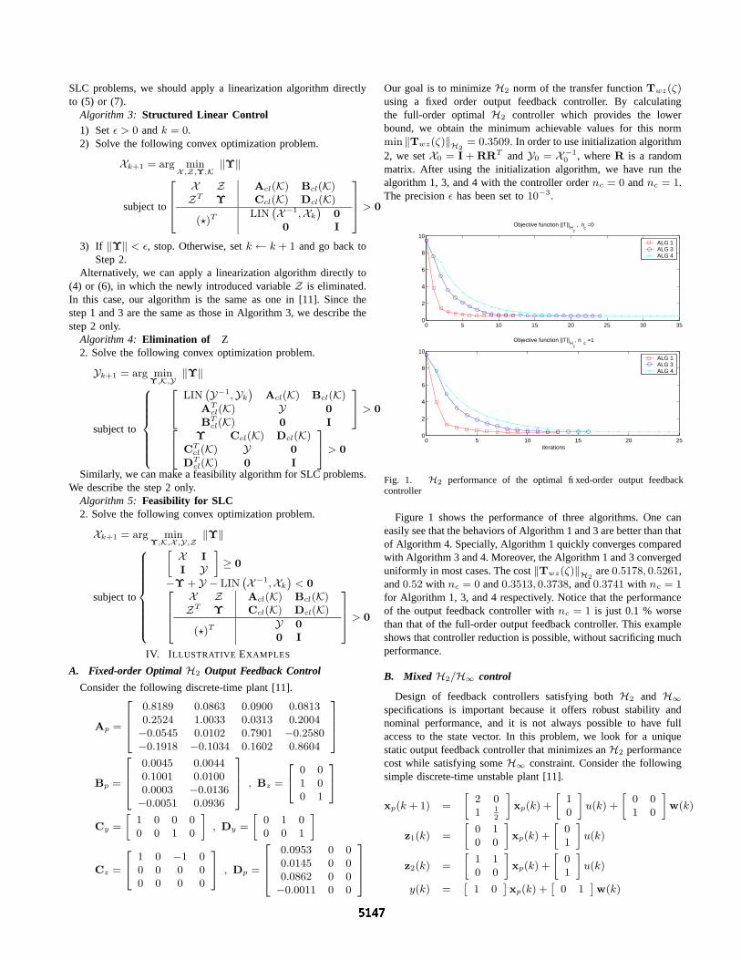
0 , where R is a randommatrix. After using the initialization algorithm, we have run thealgorithm 1, 3, and 4 with the controller order nc = 0 and nc = 1.The precision ε has been set to 10−3.

0 5 10 15 20 25 30 350

2

4

6

8

10

Objective function ||T|| H

2

, nc =0

ALG 1ALG 3ALG 4

0 5 10 15 20 250

2

4

6

8

10

Objective function ||T|| H

2

, nc =1

iterations

ALG 1ALG 3ALG 4

Fig. 1. H2 performance of the optimal fixed-order output feedbackcontroller

Figure 1 shows the performance of three algorithms. One caneasily see that the behaviors of Algorithm 1 and 3 are better than thatof Algorithm 4. Specially, Algorithm 1 quickly converges comparedwith Algorithm 3 and 4. Moreover, the Algorithm 1 and 3 convergeduniformly in most cases. The cost ‖Twz(ζ)‖H2

are 0.5178, 0.5261,and 0.52 with nc = 0 and 0.3513, 0.3738, and 0.3741 with nc = 1for Algorithm 1, 3, and 4 respectively. Notice that the performanceof the output feedback controller with nc = 1 is just 0.1 % worsethan that of the full-order output feedback controller. This exampleshows that controller reduction is possible, without sacrificing muchperformance.

B. Mixed H2/H∞ control

Design of feedback controllers satisfying both H2 and H∞

specifications is important because it offers robust stability andnominal performance, and it is not always possible to have fullaccess to the state vector. In this problem, we look for a uniquestatic output feedback controller that minimizes an H2 performancecost while satisfying some H∞ constraint. Consider the followingsimple discrete-time unstable plant [11].

xp(k + 1) =

»

2 01 1

2

–

xp(k) +

»

10

–

u(k) +

»

0 01 0

–

w(k)

z1(k) =

»

0 10 0

–

xp(k) +

»

01

–

u(k)

z2(k) =

»

1 10 0

–

xp(k) +

»

01

–

u(k)

y(k) =ˆ

1 0˜

xp(k) +ˆ

0 1˜

w(k)

By calculating the dynamic output feedback optimal H2 and H∞

controllers, we obtain the following minimum achievable values forthese norms

min ‖Twz1(ζ)‖H2

= 4.0957 , min ‖Twz2(ζ)‖H∞

= 6.3409.

Our objective is to design a static output feedback controller thatminimizes ‖Twz1

(ζ)‖H2while keeping ‖Twz2

(ζ)‖H∞

below acertain level γ. Let’s set γ = 7. Note that Algorithm 1 can beapplicable with the constraint X1 = X2 = X . Our algorithm canbe composed of three sub algorithms which are

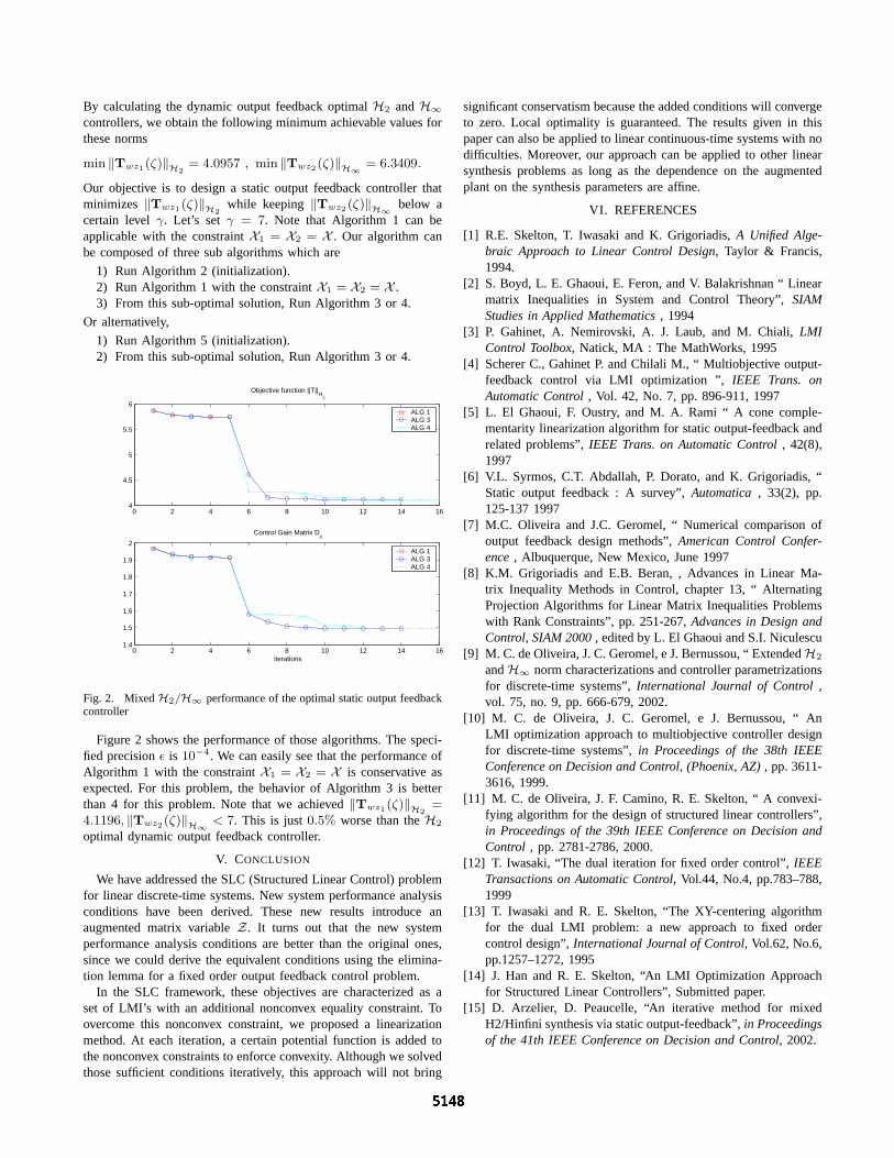
1) Run Algorithm 2 (initialization).2) Run Algorithm 1 with the constraint X1 = X2 = X .3) From this sub-optimal solution, Run Algorithm 3 or 4.

Or alternatively,

1) Run Algorithm 5 (initialization).2) From this sub-optimal solution, Run Algorithm 3 or 4.

0 2 4 6 8 10 12 14 164

4.5

5

5.5

6

Objective function ||T|| H

2

ALG 1ALG 3 ALG 4

0 2 4 6 8 10 12 14 161.4

1.5

1.6

1.7

1.8

1.9

2

Control Gain Matrix Dc

iterations

ALG 1ALG 3 ALG 4

Fig. 2. Mixed H2/H∞ performance of the optimal static output feedbackcontroller

Figure 2 shows the performance of those algorithms. The speci-fied precision ε is 10−4. We can easily see that the performance ofAlgorithm 1 with the constraint X1 = X2 = X is conservative asexpected. For this problem, the behavior of Algorithm 3 is betterthan 4 for this problem. Note that we achieved ‖Twz1

(ζ)‖H2=

4.1196, ‖Twz2(ζ)‖H∞

< 7. This is just 0.5% worse than the H2

optimal dynamic output feedback controller.

V. CONCLUSION

We have addressed the SLC (Structured Linear Control) problemfor linear discrete-time systems. New system performance analysisconditions have been derived. These new results introduce anaugmented matrix variable Z . It turns out that the new systemperformance analysis conditions are better than the original ones,since we could derive the equivalent conditions using the elimina-tion lemma for a fixed order output feedback control problem.

In the SLC framework, these objectives are characterized as aset of LMI’s with an additional nonconvex equality constraint. Toovercome this nonconvex constraint, we proposed a linearizationmethod. At each iteration, a certain potential function is added tothe nonconvex constraints to enforce convexity. Although we solvedthose sufficient conditions iteratively, this approach will not bring

significant conservatism because the added conditions will convergeto zero. Local optimality is guaranteed. The results given in thispaper can also be applied to linear continuous-time systems with nodifficulties. Moreover, our approach can be applied to other linearsynthesis problems as long as the dependence on the augmentedplant on the synthesis parameters are affine.

VI. REFERENCES

[1] R.E. Skelton, T. Iwasaki and K. Grigoriadis, A Unified Alge-braic Approach to Linear Control Design, Taylor & Francis,1994.

[2] S. Boyd, L. E. Ghaoui, E. Feron, and V. Balakrishnan “ Linearmatrix Inequalities in System and Control Theory”, SIAMStudies in Applied Mathematics , 1994

[3] P. Gahinet, A. Nemirovski, A. J. Laub, and M. Chiali, LMIControl Toolbox, Natick, MA : The MathWorks, 1995

[4] Scherer C., Gahinet P. and Chilali M., “ Multiobjective output-feedback control via LMI optimization ”, IEEE Trans. onAutomatic Control , Vol. 42, No. 7, pp. 896-911, 1997

[5] L. El Ghaoui, F. Oustry, and M. A. Rami “ A cone comple-mentarity linearization algorithm for static output-feedback andrelated problems”, IEEE Trans. on Automatic Control , 42(8),1997

[6] V.L. Syrmos, C.T. Abdallah, P. Dorato, and K. Grigoriadis, “Static output feedback : A survey”, Automatica , 33(2), pp.125-137 1997

[7] M.C. Oliveira and J.C. Geromel, “ Numerical comparison ofoutput feedback design methods”, American Control Confer-ence , Albuquerque, New Mexico, June 1997

[8] K.M. Grigoriadis and E.B. Beran, , Advances in Linear Ma-trix Inequality Methods in Control, chapter 13, “ AlternatingProjection Algorithms for Linear Matrix Inequalities Problemswith Rank Constraints”, pp. 251-267, Advances in Design andControl, SIAM 2000 , edited by L. El Ghaoui and S.I. Niculescu

[9] M. C. de Oliveira, J. C. Geromel, e J. Bernussou, “ ExtendedH2

and H∞ norm characterizations and controller parametrizationsfor discrete-time systems”, International Journal of Control ,vol. 75, no. 9, pp. 666-679, 2002.

[10] M. C. de Oliveira, J. C. Geromel, e J. Bernussou, “ AnLMI optimization approach to multiobjective controller designfor discrete-time systems”, in Proceedings of the 38th IEEEConference on Decision and Control, (Phoenix, AZ) , pp. 3611-3616, 1999.

[11] M. C. de Oliveira, J. F. Camino, R. E. Skelton, “ A convexi-fying algorithm for the design of structured linear controllers”,in Proceedings of the 39th IEEE Conference on Decision andControl , pp. 2781-2786, 2000.

[12] T. Iwasaki, “The dual iteration for fixed order control”, IEEETransactions on Automatic Control, Vol.44, No.4, pp.783–788,1999

[13] T. Iwasaki and R. E. Skelton, “The XY-centering algorithmfor the dual LMI problem: a new approach to fixed ordercontrol design”, International Journal of Control, Vol.62, No.6,pp.1257–1272, 1995

[14] J. Han and R. E. Skelton, “An LMI Optimization Approachfor Structured Linear Controllers”, Submitted paper.

[15] D. Arzelier, D. Peaucelle, “An iterative method for mixedH2/Hinfini synthesis via static output-feedback”, in Proceedingsof the 41th IEEE Conference on Decision and Control, 2002.