AN INVESTIGATION OF TWO-STAGE TESTS

AN INVESTIGATION OF TWO-STAGE TESTS

Marc Vandemeulebroecke

Otto-von-Guericke-Universitat Magdeburg

and

Schering AG

Abstract: Two-stage tests may be defined in terms of a combination func-

tion for the p-values of the separate stages, or alternatively by specifying a

conditional error function, i.e., the conditional probability for an erroneous

rejection given the first stage. Examples have been published suggesting

that these two approaches are essentially equivalent. We provide a formal

link between them that yields a general framework for two-stage tests. Our

viewpoint leads to an overall p-value notion that covers different previously

proposed concepts, and it allows an easy construction of new two-stage tests.

One particular test is further characterized.

Key words and phrases: Adaptive design, combination test, conditional error

function, interim analysis, overall p-value, two-stage test.

Date: July 14, 2005.1

AN INVESTIGATION OF TWO-STAGE TESTS 2

1. Introduction

Armitage, McPherson and Rowe (1969) quantified the inflation of the type I error in

(naive) sequential testing. Since then numerous statistical procedures have been proposed

that adjust for this inflation, especially in the field of clinical trials, seeking to maximize

flexibility in trial conduct and to minimize patient exposure or costs. The group sequential

tests of Pocock (1977) and O’Brien and Fleming (1979) were more practical than the purely

sequential, in theory optimal, Sequential Probability Ratio Test of Wald (1945) (see also

Wald and Wolfowitz (1948)). Group sequential variants were provided by DeMets and

Ware (1980, 1982), Gould and Pecore (1982) and others. Wang and Tsiatis (1987) and

Pampallona and Tsiatis (1994) generalized these procedures to the “∆-class” of group

sequential boundaries. Lan and DeMets (1983) introduced more flexibility with the alpha-

spending function approach, setting aside the need for prespecified stage sizes and allowing

an arbitrary apportionment of the type I error over the stages. Bauer (1989a) put forward

the principle of combining the p-values from separate stages. This principle permits a wide

range of data-driven design modifications, including an adaptive choice of the sample size,

the test statistic or even the null hypothesis. Two prominent examples apply combination

methods originally conceived for meta-analyses to the context of adaptive trials. Bauer and

Kohne (1994) suggested the use of Fisher’s product criterion (Fisher (1932), see also Bauer

(1989a, 1989b)). Lehmacher and Wassmer (1999) put emphasis on the inverse normal

method (Mosteller and Bush (1954), see also Bauer and Kohne (1994) and Cui, Hung

and Wang (1999)). Motivated by the wish to extend a study in order to reach a certain

conditional power (Lan, Simon and Halperin (1982)), Proschan and Hunsberger (1995)

proposed to define a two-stage test by a conditional error function. This function specifies

the conditional probability for an erroneous rejection of the null hypothesis given the first


stage. More recent works include the “self-designing trials” of Fisher (1998) and Shen

and Fisher (1999); modifications of the Proschan-Hunsberger procedure by Liu and Chi

(2001) and Li, Shih, Xie and Lu (2002); adaptive multistage designs by Muller and Scha-

fer (2001) and Brannath, Posch and Bauer (2002); and lately, an interesting geometrical

characterization of two-stage tests by Proschan (2003).

All these approaches are interrelated to a greater or lesser extent, as has been pointed

out by Posch and Bauer (1999), Wassmer (1999, 2000), Bauer, Brannath and Posch (2001),

and Jennison and Turnbull (2003) among others. In the context of trials with only two

stages, Posch and Bauer (1999) and Wassmer (1999, 2000) presented examples that suggest

a general correspondence between a conditional error function and a function that combines

two p-values in the spirit of Bauer (1989a). The idea of this general correspondence is

commonly accepted, but its nature has not yet been thoroughly explored. This is the first

purpose of the present article. We show that a p-value combination function corresponds in

fact to a whole family of conditional error functions, specifying level-α-tests for each level

α between 0 and 1. Based on this link, our second focus lies in defining overall p-values

for two-stage tests. Overall p-values are of interest as a “measure of certainty” and may

be used to construct multistage tests by recursive combination as presented by Brannath,

Posch and Bauer (2002). Previous definitions based on a p-value combination function

(Brannath, Posch and Bauer (2002)) or a family of conditional error functions (Liu and

Chi (2001)) fit in our framework. Finally, and this is our third point, we illustrate that our

concept allows an easy construction of new two-stage tests and a more flexible handling of

known two-stage tests.

We hope to contribute to the understanding of two-stage tests by providing a general,

formally rigorous and geometrically intuitive framework that covers several previously pro-

posed concepts. The rest of this paper is organized as follows. Section 2 recapitulates


the p-value combination function approach and the conditional error function approach. A

formal link between these approaches is provided in Section 3. Overall p-values are the

subject of Section 4, followed by an example in Section 5. Section 6 completes the arti-

cle with a brief discussion. Technical details and key steps of proof are provided in three

appendices. To avoid problems with conflicting directional decisions, we assume one-sided

testing throughout. Integrals are taken over the unit interval unless otherwise specified.

2. Two approaches

A two-stage procedure for testing a null hypothesis H0 may be defined in terms of

the overall level α, stopping bounds α1 and α0, a parameter α2 and a function C( · , · ) to

combine the p-values of the two stages. The bound α1 is the local level of the test based on

the first stage. The parameter α2 is the local level of the test based on both stages, ignoring

the two-stage nature of the design. The quantities α, α0 and α1 are subject to the condition

0 ≤ α1 ≤ α ≤ α0 ≤ 1, and C must have some regularity properties that will be defined

later. After computing the p-value p1 of the first stage, the test stops with rejection of H0 if

p1 ≤ α1, and it stops without rejection of H0 (“for futility”) if p1 > α0. If α1 < p1 ≤ α0, the

test proceeds, the p-value p2 of the second stage is computed, and the “combination test”

is carried out. H0 is then rejected if and only if C(p1, p2) is not greater than some threshold

c(α2) that is determined by the local level α2 of this combination test. Given C, the choice

of α0, α1 and c(α2) is constrained by the desired overall level α for the two-stage procedure,

assuming that p1 and p2 are independent and uniformly distributed on [0, 1] under H0. As

Bauer (1989a) pointed out, however, this assumption is not necessary for the level α to be

kept. It suffices that under H0 the distribution of p1 and the conditional distribution of p2

given p1 are stochastically not smaller than the uniform distribution on [0, 1]. Brannath,

Posch and Bauer (2002) called this property p-clud. The rejection region of such a test can


be visualized as the area

{p1 ≤ α1} ∪ ({C(p1, p2) ≤ c(α2)} ∩ {p1 ≤ α0})

in the unit square. Choosing α0 = α = α1 yields a single stage test as a special case.

This idea of combining the p-values from separate stages was put forward by Bauer

(1989a). As an example, Bauer and Kohne (1994) and Bauer and Rohmel (1995) proposed

the choice of C(p1, p2) = p1p2, yielding c(α2) = exp(−χ24,α2

/2) (Fisher (1932)) which is

traditionally written as cα2 . By χ24,α2

we denote the (1 − α2)-quantile of the central χ2-

distribution with 4 degrees of freedom. Supposing cα2 ≤ α1, the parameters need to satisfy

α1 + cα2(ln α0 − ln α1) = α for an overall test level of α. We refer to this test as Fisher’s

combination test.

An alternative approach, originally posed by Proschan and Hunsberger (1995), defines

a two-stage test by specifying its conditional error function, i.e., the conditional probability

for an erroneous rejection given the first stage. Following Wassmer (1999, 2000), we write

this function as a function in p1. Any nonincreasing function α with values in [0, 1] may be

used. For technical reasons we additionally assume α to be left continuous. In this approach

the same testing procedure is implemented as in the p-value combination function approach,

with the combination test criterion C(p1, p2) ≤ c(α2) replaced by p2 ≤ α(p1). That is, α,

α0 and α1 are chosen to satisfy 0 ≤ α1 ≤ α ≤ α0 ≤ 1. If p1 ≤ α1 or p1 > α0, the test

stops after the first stage, with or without rejection of H0, respectively. Otherwise, H0 is

rejected if and only if p2 ≤ α(p1). We can set α2 =∫

α(p1) dp1, and the interpretation of

all parameters is the same as in the p-value combination function approach. The choice of

the parameters is constrained by α1 +∫ α0

α1α(p1) dp1 = α, and the rejection region in the

unit square is now

{p1 ≤ α1} ∪ ({p2 ≤ α(p1)} ∩ {p1 ≤ α0}).


Again, the constraining equation makes use of the assumption that p1 and p2 are inde-

pendent and uniformly distributed on [0, 1] under H0. The procedure still keeps the level α

if p1 and p2 are p-clud under H0. Note that α1 and α0 are imposed on α rather than being

part of it. In a common alternative notation, max{p1; α(p1) = 1} and inf{p1; α(p1) = 0}

take over the roles of α1 and α0, respectively, and the choice of α is constrained by

∫α(p1) dp1 = α. In our view, however, this obscures the analogy between the two ap-

proaches.

For example, α(p1) = min{1, cα2/p1} is a conditional error function that depends on α2.

Together with α, α0 and α1, constrained by α1 +∫ α0

α1α(p1) dp1 = α1 + cα2(ln α0− ln α1) = α

(and cα2 ≤ α1), it specifies a two-stage test.

Clearly, this test is identical to Fisher’s combination test. This and other examples,

first presented by Posch and Bauer (1999) and Wassmer (1999, 2000), have led to the

common understanding that the two approaches complement one another. The next section

investigates their relationship in a formal way in a general setting.

3. A formal framework for two-stage tests

To motivate the definitions that follow, imagine p1 and p2 are combined by some function

C that is continuous and strictly increasing in both arguments. C defines a “rising surface”

over the unit square, and the null hypothesis is rejected if C(p1, p2) does not exceed some

prespecified height H = c(α2) (early stopping not considered). The level curve {C(p1, p2) =

H} may be thought of as the boundary of the rejection region {C(p1, p2) ≤ H}. We can

write this level curve as a function αH in p1. For a given value p1, the null hypothesis is

then rejected if p2 ≤ αH(p1), due to the monotonicity properties of C. Figure 1 illustrates

this idea for Fisher’s combination test. Assuming p2 is uniformly distributed on [0, 1], the


conditional rejection probability given p1 is Pr(p2 ≤ αH(p1)) = αH(p1). Thus, αH is the

conditional error function.

— Please insert Figure 1 about here —

However, this reasoning is not always applicable in a straightforward way. In Figure

1, for example, the level curve αH is not defined over the entire unit interval. In a more

general situation, C may not be continuous, or it may have constant regions, and the

level sets {C(p1, p2) = H} can have unusual shapes. Conversely, it is not clear how to

find a combination function C that “corresponds” to a given conditional error function.

A generalization of the level curve idea is needed. For this purpose we now develop the

following framework.

We call any function C : (0, 1)2 → R a p-value combination function if C( · , p2) is

nondecreasing and left continuous for all p2 ∈ (0, 1), and C(p1, · ) is nondecreasing for all

p1 ∈ (0, 1). By a conditional error function we mean any nonincreasing and left continuous

function α : (0, 1) → [0, 1]. Properties 1–3 follow by elementary arguments.

Property 1. For any p-value combination function C, αH(p1) = max{sup[p2 ∈ (0, 1);

C(p1, p2) ≤ H], 0} defines a conditional error function for every H ∈ R. (We use the con-

vention sup(∅) = −∞.) If H ≤ H ′, then αH ≤ αH′on (0, 1). We have αH ≤ αH′

on (0, 1)

if and only if∫

αH(p1) dp1 ≤∫

αH′(p1) dp1, so the family (αH)H may be reparameterized

as (αh)h such that h =∫

αh(p1) dp1. Here, αh 6= αh′ for any h 6= h′. The function α0 (α1)

will exist if and only if C is bounded from below (above); otherwise define α0 = 0 (α1 = 1)

on (0, 1). The entire mapping is denoted by α, that is, (αh)h = α(C).

Property 2. Let a = (αh)h∈[0,1] be a family of conditional error functions satisfying h =

∫αh(p1) dp1 for all h, and αh ≤ αh′ on (0, 1) for any h ≤ h′. Then C(p1, p2) = min{h ∈


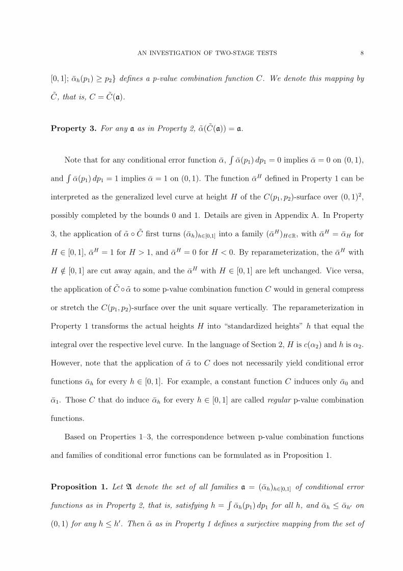
[0, 1]; αh(p1) ≥ p2} defines a p-value combination function C. We denote this mapping by

C, that is, C = C(a).

Property 3. For any a as in Property 2, α(C(a)) = a.

Note that for any conditional error function α,∫

α(p1) dp1 = 0 implies α = 0 on (0, 1),

and∫

α(p1) dp1 = 1 implies α = 1 on (0, 1). The function αH defined in Property 1 can be

interpreted as the generalized level curve at height H of the C(p1, p2)-surface over (0, 1)2,

possibly completed by the bounds 0 and 1. Details are given in Appendix A. In Property

3, the application of α ◦ C first turns (αh)h∈[0,1] into a family (αH)H∈R, with αH = αH for

H ∈ [0, 1], αH = 1 for H > 1, and αH = 0 for H < 0. By reparameterization, the αH with

H /∈ [0, 1] are cut away again, and the αH with H ∈ [0, 1] are left unchanged. Vice versa,

the application of C ◦ α to some p-value combination function C would in general compress

or stretch the C(p1, p2)-surface over the unit square vertically. The reparameterization in

Property 1 transforms the actual heights H into “standardized heights” h that equal the

integral over the respective level curve. In the language of Section 2, H is c(α2) and h is α2.

However, note that the application of α to C does not necessarily yield conditional error

functions αh for every h ∈ [0, 1]. For example, a constant function C induces only α0 and

α1. Those C that do induce αh for every h ∈ [0, 1] are called regular p-value combination

functions.

Based on Properties 1–3, the correspondence between p-value combination functions

and families of conditional error functions can be formulated as in Proposition 1.

Proposition 1. Let A denote the set of all families a = (αh)h∈[0,1] of conditional error

functions as in Property 2, that is, satisfying h =∫

αh(p1) dp1 for all h, and αh ≤ αh′ on

(0, 1) for any h ≤ h′. Then α as in Property 1 defines a surjective mapping from the set of


all regular p-value combination functions C onto A. This mapping reduces to a bijection if

we identify any C, C ′ with α(C) = α(C ′).

In simple terms, A provides special ways of filling the unit square, conveniently pa-

rameterized by the own integral. Figure 2 illustrates this for Fisher’s combination test.

The p-value combination function C(p1, p2) = p1p2 induces the family (αH)H∈R defined by

αH(p1) = max{0, min{1, H/p1}}. It can be reparameterized as (αα2)α2∈[0,1], with αα2(p1) =

min{1, cα2/p1} for 0 < α2 < 1, α0 = 0, and α1 = 1. The αα2 describe the level curves of

the p1p2-surface over the unit square, completed by the upper bound 1. The parameter

α2 equals the integral∫

αα2(p1) dp1. Note that it is not required that every point in the

unit square lies on exactly one of the curves. Infinitely many curves pass through (p1, p2)

if p2 = 1. Or consider the family specified by αh = 1[0,h], h ∈ [0, 1], where 1[0,h](p1) equals

1 if p1 ∈ [0, h], and 0 otherwise. Those (p1, p2) with p2 ∈ (0, 1) lie on none of the curves.


It is important to realize that it does not matter whether the way the unit square is

filled stems from a p-value combination function or not. Based on any a = (αh)h∈[0,1] ∈ A,

a two-stage test is implemented as follows.

Method 1. Select α, α0, α1 and α2 ∈ [0, 1] that satisfy 0 ≤ α1 ≤ α ≤ α0 ≤ 1 and the

level condition α1 +∫ α0

α1αα2(p1) dp1 = α. Observe the first stage. If p1 ≤ α1 or p1 > α0,

then stop with or without rejection of the null hypothesis, respectively. Otherwise conduct

the second stage, and reject the null hypothesis if and only if p2 ≤ αα2(p1).

This is the conditional error function approach introduced in the previous section, with

α = αα2 . The test keeps the level α if p1 and p2 are p-clud under the null hypothesis, and it

has exact level α if p1 and p2 are independent and uniformly distributed on [0, 1] under the


null hypothesis. In particular, a two-stage test with an arbitrarily chosen level α ∈ [0, 1]

can always be constructed. Finally, consider the case that the underlying a ∈ A has been

induced by a p-value combination function C. Then, by Appendix A (1), we can replace

the condition p2 ≤ αα2(p1) in Method 1 by C(p1, p2) ≤ c(α2), provided that C(p1, · ) is left

continuous for all p1. This completes the connection between the two approaches.

Chi and Liu (1999) proposed the same idea of filling the unit square by some suitable

family of conditional error functions. They used this concept to design mid-trial sample

size re-estimation in case of a misspecified anticipated treatment effect, rather than being

motivated by a connection to the p-value combination function approach. The properties

required for their conditional error function families differ from those proposed here. In

particular, for Fisher’s combination test, they concluded that a way their requirements

would be “simultaneously satisfied is not readily apparent” (Liu and Chi (2001)). In our

framework the corresponding family is easily specified, as sketched after Proposition 1 and

illustrated in Figures 1 and 2.

The inverse normal method (Lehmacher and Wassmer (1999), see also Posch and Bauer

(1999) and Wassmer (1999, 2000)) serves as another example. In our notation it is repre-

sented by

CINM(p1, p2) =(Φ−1(p1) + Φ−1(p2)

)/√

2,

αINMα2

(p1) =

0 if α2 = 0,

Φ(√

2 Φ−1(α2)− Φ−1(p1))

if 0 < α2 < 1,

1 if α2 = 1,

where Φ denotes the distribution function of the standard normal distribution, and cINM(α2) =

Φ−1(α2). Note that, according to Method 1, for a fixed level α the three design parameters

α0, α1 and α2 interact due to the level condition, but there is no interdependence of just two


of them. For example, we may want to fix α1 (and α). Then we are still free to manipulate

α0 and α2. This is not possible in the classical formulation of the inverse normal method,

where α1 and α2 are directly linked (Li, Shih, Xie and Lu (2002) pointed out the same for

their procedure). Thus, Method 1 can not only be used to define new two-stage tests, but

also to make known two-stage tests more flexible.

4. Overall p-values for two-stage tests

If overall p-values are available for two-stage tests, then multistage tests can be con-

structed by recursive combination. Brannath, Posch and Bauer (2002) presented this idea.

In a two-stage test, the p-value p2 of the second stage may itself be the overall p-value of

another two-stage test. The second stage of this latter test may again be performed in two

stages, and so on. Brannath, Posch and Bauer defined an overall p-value function based on

the combination function C. They also noted that other p-value functions can be used, and

alluded to a proposal by Liu and Chi (2001) that is based on a family of conditional error

functions. Here, the idea of Liu and Chi will be used to define overall p-values within the

framework of the previous section; the notion of Brannath, Posch and Bauer may be viewed

as a special case. The concept is similar to what Fairbanks and Madsen (1982) proposed in

the group sequential setting, and the sample space ordering in the sense of Tsiatis, Rosner

and Mehta (1984) is respected.

Lacking a general formal definition, p-values are commonly conceived to represent one

of two things (or both): the probability under the null hypothesis of getting observations

at least as extreme as the ones actually observed, or the lowest level at which a selected

test still rejects the null hypothesis. The latter concept presupposes the availability of

a test for each possible level. The former concept requires—in the context of two-stage

tests—the specification of what is “at least as extreme” as an observed (p1, p2) in the unit


square. Is it any (p′1, p′2) with p′1 + p′2 ≤ p1 + p2, or maybe p′1p

′2 ≤ p1p2? A more general

approach would be to fill the unit square by a family of conditional error functions, to select

the function that passes through (p1, p2), and to call the area below (and including) this

function “at least as extreme”. In other words, both concepts require an element (αh)h∈[0,1]

of A. On (αh)h∈[0,1] we additionally impose early stopping bounds α0 and α1 that are, unlike

in Method 1, assumed to be the same for all αh. More formally:

Definition 1. For a = (αh)h∈[0,1] ∈ A and 0 ≤ α1 ≤ α0 ≤ 1, the function p : [0, 1]2 → [0, 1],

p(p1, p2) =

p1 if p1 ≤ α1 or p1 > α0,

α1 +∫ α0

α1αh?(x) dx otherwise,

with h? = C(a)(p1, p2) = min{h ∈ [0, 1]; αh(p1) ≥ p2} as defined in Property 2, is called

the overall p-value (function).

Note that if α1 = 0 and α0 = 1, then p = C(a) on (0, 1)2. By Property 3, any a ∈ A

may thus be interpreted as the family of level curves of its own overall p-value function.

Fisher’s combination test, as depicted in Figure 2, again serves as an illustration. Sup-

pose α1 = 0.0845 and α0 = 0.5 (yielding an overall test level of α = 0.1 if α2 = 0.05). If

p1 = 0.2 and p2 = 0.15, then h for which αh(p1) ≥ p2 barely occurs is h? =∫

α0.03(x) dx,

and the overall p-value is 0.0845+∫ 0.5

0.0845α0.03(x) dx = 0.0845+0.03{ln(0.5)− ln(0.0845)} =

0.1378.

Definition 1 is inspired by Liu and Chi (2001), but it remains sensible when there is no

αh passing through (p1, p2), and also when there is more than one such αh. Presupposing

the availability of a two-stage test for each possible level, Liu and Chi proved that a two-

stage level α test is equivalent to checking whether its overall p-value is not greater than

α, and that by this property, the overall p-value is unique. In our terms, this is because

the presupposed tests and the definition of the overall p-value are both based on the same


choice of how to fill the unit square, i.e., the same choice of a ∈ A. This is formulated more

precisely in the following lemma.

Lemma 1. Let (αh)h∈[0,1] ∈ A, 0 ≤ α1 ≤ α0 ≤ 1, α ∈ [0, 1] and (p1, p2) ∈ [0, 1]2.

(1) If α /∈ [α1, α0], or α ∈ [α1, α0] and p1 /∈ (α1, α0], then p(p1, p2) ≤ α if and only if

p1 ≤ α.

(2) If α ∈ [α1, α0] and p1 ∈ (α1, α0], then p(p1, p2) ≤ α if and only if p2 ≤ αα2(p1),

where α2 is arbitrary in [0, 1] with α1 +∫ α0

α1αα2(x) dx = α. An α2 satisfying this

condition always exists, and for any two such α2 and α′2, αα2 = αα′2 on (α1, α0].

Therefore, assuming α ∈ [α1, α0], Method 1 is equivalent to rejecting the null hypothesis

if and only if p(p1, p2) ≤ α. The case α /∈ [α1, α0] is included in Lemma 1 with regard to

Proposition 2.

Proposition 2. If p1 and p2 are independent and uniformly distributed on [0, 1], then

p(p1, p2) is uniformly distributed on [0, 1]. If p1 and p2 are p-clud, then the distribution of

p(p1, p2) is stochastically not smaller than the uniform distribution on [0, 1].

Proposition 2 has an important implication. The recursive combination principle of

Brannath, Posch and Bauer (2002) is applicable, and multistage tests can be constructed.

The overall p-value function proposed by the same authors was based on the combina-

tion function C. Property 4 shows that it coincides with our notion in a special case.

Property 4. Let a ∈ A be induced by a p-value combination function C such that C(p1, · )

is left continuous for all p1 ∈ (0, 1). The overall p-value can then be written as

p(p1, p2) =

p1 if p1 ≤ α1 or p1 > α0,

α1 +∫ α0

α1

∫ 1

01{C(x,y)≤C(p1,p2)} dy dx otherwise,


where 1{C(x,y)≤C(p1,p2)} equals 1 if C(x, y) ≤ C(p1, p2), and 0 otherwise.

5. Example

We emphasize the idea of viewing a two-stage test as a family of conditional error func-

tions that fills the unit square. According to Proposition 1, a (regular) p-value combination

function C contains “too much” information: only the (generalized) level curves of the

C(p1, p2)-surface are of interest. On the other hand, a single conditional error function α

is obviously “not enough”. Only a family a ∈ A provides the means to construct two-stage

tests to any level, and to define overall-p-values for two-stage tests.

Clearly, there are many ways to specify such a family. For instance, the most prominent

conditional error functions, such as for Fisher’s combination test or the inverse normal

method, are already given as families. Alternatively, we may want to “extend” a single

conditional error function α to a family. This can be done in numerous ways, but it might

be reasonable to pick an extension method that mimics the structure of a well-established

test in some sense. As regards Fisher’s combination test, this is particularly easy: define

αr(x) = (α(xr))1/r for r > 0. When reparameterized by their integrals and completed by

the constants α0 = 0 and α1 = 1, these functions form an element a of A (except if α = 0 or

α = 1). In this context, however, it is more convenient to stick with the parameterization

by r > 0. Indeed, Fisher’s combination test is closed under this transformation. Starting

with any conditional error function α(x) = min{1, cα2/x} to a particular level α2, the whole

family is restored by αr(x) = min{1, c1/rα2 /x}, r > 0.

If the initial function α is not given, we are free to choose it as well. Following Adcock

(1960), we may want the p-values of the two stages to cancel out in a symmetric fashion if

early stopping is not considered: p2 = 1−p1 should result in an overall p-value of 0.5. Thus,

we apply the above transformation to the diagonal y = 1 − x. This yields the functions


αr(x) = (1− xr)1/r, r > 0. A two-stage test based on this family is implemented according

to Method 1, with the condition p2 ≤ αα2(p1) written as pr(α2)1 + p

r(α2)2 ≤ 1, and r(α2) > 0

such that∫

(1 − xr(α2))1/r(α2) dx = α2. Table 1 compares this new procedure to Fisher’s

combination test and the inverse normal method. It shows α1 depending on α0 and on the

apportionment of α over the stages, to satisfy the level condition in Method 1 for the level

α = 0.05. The case α0 = 0.5 corresponds to stopping for futility after the first stage if the

observed effect shows in the wrong direction. The case α0 = 1 prohibits any stopping for

futility. If α2 = α, the full level is used after the final stage; if α2 = α1, the same local level

is used after both stages (this is the “Pocock-type”).

— Please insert Table 1 about here —


Note the similarity between the inverse normal method and the new test, especially for

the Pocock-type. Indeed, the underlying families of conditional error functions look almost

identical, as shown in Figure 3. If the full level α is used after the second stage and no

stopping for futility is allowed (α2 = α and α0 = 1), these two tests never stop after the first

stage. In the same situation, Fisher’s combination test always rejects the null hypothesis

when p1 ≤ 0.0087, and, strictly speaking, 0.0087 is just an upper bound (but of course a

sensible choice) for α1.

Tables 2 and 3 provide α1 for the new test in a wider range of situations. The case

α1 = α = α0 = 0.1 is a single stage test. Particularly in the Pocock-type, α0 matters only

when small. This is because the area under the conditional error function becomes very

small towards the right side of the unit square.

— Please insert Tables 2 and 3 about here —


6. Discussion

Adaptive tests offer great flexibility in the planning and conduct of, for example, clinical

trials. In recent times, procedures have been developed that do not even require a full

prespecification of the test statistic or of the null hypothesis. While desirable in theory, such

flexibility may be dangerous in practice. It does not open the door to total arbitrariness,

but actually requires even more careful study planning. The issue to be answered by the

study should be thoroughly formulated. Still, when responsibly used, adaptive tests are a

very versatile and practical tool.

The current article provides a formal link between two approaches to adaptive two-

stage tests, namely, the p-value combination function approach and the conditional error

function approach, in a general framework. The main idea is to view a two-stage test as a

family of conditional error functions that fills the unit square. This family is used to define

overall p-values in a way that covers previously given definitions based on either of the two

approaches. In addition, new two-stage tests can be specified based on the same reasoning.

The construction of multistage tests is possible by recursive combination as described by

Brannath, Posch and Bauer (2002). These authors also outline the principles to construct

point estimates and confidence intervals.

It is understood that the properties of a two-stage test and the meaningfulness of an

overall p-value are highly dependent on the choice of the underlying family of conditional

error functions. This family can have a vast variety of shapes. It remains to be explored

which choices are advantageous from a practical perspective (see Brannath and Bauer (2004)

for an investigation on “optimal” conditional error functions).


Acknowledgements

The author would like to thank two anonymous referees for their thorough review and

helpful comments. He is also grateful to Rainer Schwabe (Otto-von-Guericke-Universitat

Magdeburg) for his very valuable suggestions.

Appendix A. Generalized level curves

The following points provide an insight into the relationship between a p-value combi-

nation function C and the corresponding conditional error functions αH , H ∈ R, as defined

in Property 1.

(1) C(p1, p2) ≤ H implies p2 ≤ αH(p1). The converse is true if C(p1, · ) is left continuous.

(2) C(p1, p2) ≥ H implies p2 ≥ αH(p1) if C(p1, · ) is strictly increasing. The converse is

true if C(p1, · ) is right continuous.

(3) If C(p1, · ) is continuous and strictly increasing, then

αH(p1) =

0 if C(p1, p2) > H for all p2 ∈ (0, 1),

p2 if there is a p2 ∈ (0, 1) with C(p1, p2) = H

(any p2 satisfying this condition is unique),

1 if C(p1, p2) < H for all p2 ∈ (0, 1).

Appendix B. The boundary of the unit square

Technical difficulties can arise for p1 ∈ {0, 1} or p2 ∈ {0, 1}. For example, Method 1

does not cover the case p1 = α0 = 1 since the αh are defined only on (0, 1). Similar problems

appear in the context of overall p-values in Section 4. In many cases these difficulties can

be avoided by defining C on [0, 1]2 or α on [0, 1]. We have settled for the smaller domains

because this yields the link between the p-value combination function approach and the

conditional error function approach in the most general form. It also covers such examples


as the inverse normal method, where C tends to infinity towards the boundary of the unit

square. In most applications this type of problem occurs only with probability 0.

Appendix C. Proofs

We write xn ↑ x (xn ↓ x) if a sequence (xn)n is nondecreasing (nonincreasing) and

convergent with limit x.

C.1. Proof of Property 1. The function αH is nonincreasing since C( · , p2) is non-

decreasing for all p2. To show that αH is left continuous, take a sequence pn ↑ p1.

Then αH(p1) ≤ lim αH(pn). If αH(p1) < lim αH(pn), there would be some p2 such that

αH(p1) < p2 < αH(pn), and thus C(p1, p2) > H and C(pn, p2) ≤ H, for all n. This,

however, cannot be since C( · , p2) is left continuous.

If H ≤ H ′, then clearly αH ≤ αH′. We finally show that

∫αH(p1) dp1 ≤

∫αH′

(p1) dp1

implies αH ≤ αH′; the converse is obvious. Take p such that αH′

(p) < αH(p), and let

ε = (αH(p) − αH′(p))/2. Necessarily H ′ ≤ H and αH′ ≤ αH . Since αH′

is left continuous,

there exists p′ < p such that αH′(p1) < αH(p)− ε for all p1 ∈ [p′, p]. Thus,

∫ p

p′ αH′

(p1) dp1 <

αH(p)(p− p′) ≤ ∫ p

p′ αH(p1) dp1, and therefore

∫αH′

(p1) dp1 <∫

αH(p1) dp1.

The remark about existence of α0 or α1 is straightforward to prove.

C.2. Proof of Property 2. Let C(p1, p2) = inf{h ∈ [0, 1]; αh(p1) ≥ p2}. It is easily seen

that C cannot be infinite, and that it is nondecreasing in both arguments. To show that

C( · , p2) is left continuous, take a sequence pn ↑ p1. Then lim C(pn, p2) ≤ C(p1, p2). If

lim C(pn, p2) < C(p1, p2), there would be some h such that C(pn, p2) < h < C(p1, p2), and

thus αh(pn) ≥ p2 and αh(p1) < p2, for all n. But this cannot be since αh is left continuous.

Using the left continuity of the αh, it can be shown that αh(p1) is a right continuous

function in h for fixed p1. Therefore, C(p1, p2) = min{h ∈ [0, 1]; αh(p1) ≥ p2}.


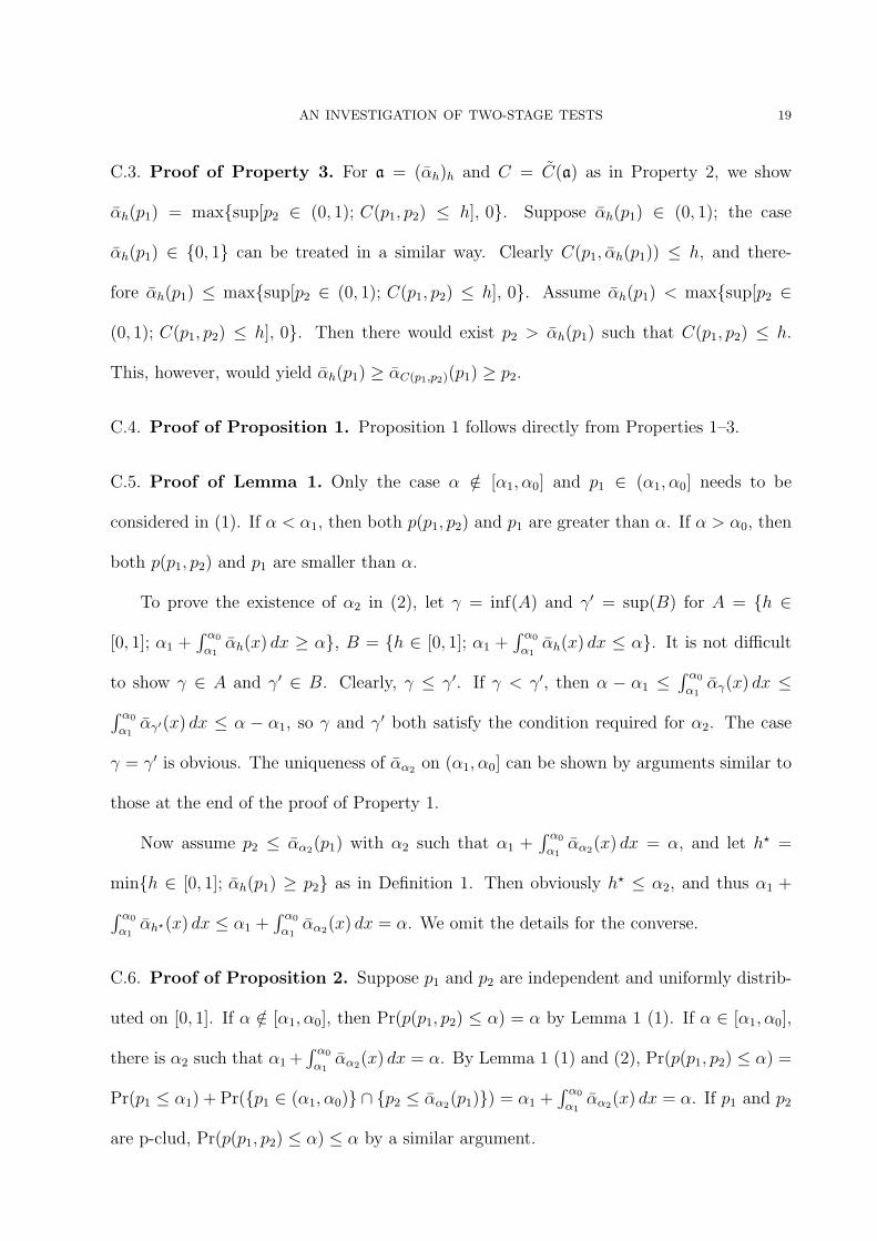
C.3. Proof of Property 3. For a = (αh)h and C = C(a) as in Property 2, we show

αh(p1) = max{sup[p2 ∈ (0, 1); C(p1, p2) ≤ h], 0}. Suppose αh(p1) ∈ (0, 1); the case

αh(p1) ∈ {0, 1} can be treated in a similar way. Clearly C(p1, αh(p1)) ≤ h, and there-

fore αh(p1) ≤ max{sup[p2 ∈ (0, 1); C(p1, p2) ≤ h], 0}. Assume αh(p1) < max{sup[p2 ∈

(0, 1); C(p1, p2) ≤ h], 0}. Then there would exist p2 > αh(p1) such that C(p1, p2) ≤ h.

This, however, would yield αh(p1) ≥ αC(p1,p2)(p1) ≥ p2.

C.4. Proof of Proposition 1. Proposition 1 follows directly from Properties 1–3.

C.5. Proof of Lemma 1. Only the case α /∈ [α1, α0] and p1 ∈ (α1, α0] needs to be

considered in (1). If α < α1, then both p(p1, p2) and p1 are greater than α. If α > α0, then

both p(p1, p2) and p1 are smaller than α.

To prove the existence of α2 in (2), let γ = inf(A) and γ′ = sup(B) for A = {h ∈

[0, 1]; α1 +∫ α0

α1αh(x) dx ≥ α}, B = {h ∈ [0, 1]; α1 +

∫ α0

α1αh(x) dx ≤ α}. It is not difficult

to show γ ∈ A and γ′ ∈ B. Clearly, γ ≤ γ′. If γ < γ′, then α − α1 ≤∫ α0

α1αγ(x) dx ≤

∫ α0

α1αγ′(x) dx ≤ α − α1, so γ and γ′ both satisfy the condition required for α2. The case

γ = γ′ is obvious. The uniqueness of αα2 on (α1, α0] can be shown by arguments similar to

those at the end of the proof of Property 1.

Now assume p2 ≤ αα2(p1) with α2 such that α1 +∫ α0

α1αα2(x) dx = α, and let h? =

min{h ∈ [0, 1]; αh(p1) ≥ p2} as in Definition 1. Then obviously h? ≤ α2, and thus α1 +

∫ α0

α1αh?(x) dx ≤ α1 +

∫ α0

α1αα2(x) dx = α. We omit the details for the converse.

C.6. Proof of Proposition 2. Suppose p1 and p2 are independent and uniformly distrib-

uted on [0, 1]. If α /∈ [α1, α0], then Pr(p(p1, p2) ≤ α) = α by Lemma 1 (1). If α ∈ [α1, α0],

there is α2 such that α1 +∫ α0

α1αα2(x) dx = α. By Lemma 1 (1) and (2), Pr(p(p1, p2) ≤ α) =

Pr(p1 ≤ α1) + Pr({p1 ∈ (α1, α0)} ∩ {p2 ≤ αα2(p1)}) = α1 +∫ α0

α1αα2(x) dx = α. If p1 and p2

are p-clud, Pr(p(p1, p2) ≤ α) ≤ α by a similar argument.


C.7. Proof of Property 4. Let h? = min{h ∈ [0, 1]; αh(p1) ≥ p2} and H = C(p1, p2). By

Appendix A (1) it can be shown that h? =∫

αH(x) dx, and for p1 ∈ (α1, α0],

p(p1, p2) = α1 +∫ α0

α1αh?(x) dx

= α1 +∫ α0

α1αH(x) dx

= α1 +∫ α0

α1

∫ 1

01{y≤αH(x)} dy dx

= α1 +∫ α0

α1

∫ 1

01{C(x,y)≤H} dy dx.

C.8. Proof of Appendix A. To show (1), note that C(p1, p2) ≤ H implies p2 ≤ αH(p1)

by the definition of αH . Now let C(p1, · ) be left continuous, and suppose p2 ≤ αH(p1). If

p2 < αH(p1), there is some p′2 > p2 with C(p1, p′2) ≤ H, so C(p1, p2) ≤ C(p1, p

′2) ≤ H. If

p2 = αH(p1), take a sequence pn ↑ p2 with C(p1, pn) ≤ H for all n. Since C(p1, · ) is left

continuous, C(p1, p2) ≤ H. (2) can be shown similarly. If C(p1, · ) is continuous and strictly

increasing, then p2 = αH(p1) ⇔ C(p1, p2) = H due to (1) and (2). This proves (3).

References

Adcock, C. J. (1960). A note on combining probabilities. Psychometrika 25, 303–305.

Armitage, P., McPherson, C. K., and Rowe, B. C. (1969). Repeated significance tests on

accumulating data. J. Roy. Statist. Soc. A 132, 235–244.

Bauer, P. (1989a). Multistage testing with adaptive designs (with discussion). Biom. und

Inform. in Med. und Biol. 20, 130–148.

Bauer, P. (1989b). Sequential tests of hypotheses in consecutive trials. Biometrical J. 31,

663–676.

Bauer, P., Brannath, W., and Posch, M. (2001). Flexible two-stage designs: an overview.

Methods Inf. Med. 40, 117–121.


Bauer, P., and Kohne, K. (1994). Evaluation of experiments with adaptive interim analyses.

Biometrics 50, 1029–1041. Correction in Biometrics 52 (1996), 380.

Bauer, P., and Rohmel, J. (1995). An adaptive method for establishing a dose-response

relationship. Statist. Medicine 14, 1595–1607.

Brannath, W., and Bauer, P. (2004). Optimal conditional error functions for the control of

conditional power. Biometrics 60, 715–723.

Brannath, W., Posch, M., and Bauer, P. (2002). Recursive combination tests. J. Amer.

Statist. Assoc. 97, 236–244.

Chi, G. Y. H., and Liu, Q. (1999). The attractiveness of the concept of a prospectively

designed two-stage clinical trial. J. Biopharm. Statist. 9, 537–547.

Cui, L., Hung, H. M. J., and Wang, S.-J. (1999). Modification of sample size in group

sequential clinical trials. Biometrics 55, 853–857.

DeMets, D. L., and Ware, J. H. (1980). Group sequential methods for clinical trials with a

one-sided hypothesis. Biometrika 67, 651–660.

DeMets, D. L., and Ware, J. H. (1982). Asymmetric group sequential boundaries for

monitoring clinical trials. Biometrika 69, 661–663.

Fairbanks, K., and Madsen, R. (1982). P values for tests using a repeated significance test

design. Biometrika 69, 69–74.

Fisher, L. D. (1998). Self-designing clinical trials. Statist. Medicine 17, 1551–1562.

Fisher, R. A. (1932). Statistical methods for research workers. Oliver & Boyd, London.

Gould, A. L., and Pecore, V. J. (1982). Group sequential methods for clinical trials allowing

early acceptance of H0 and incorporating costs. Biometrika 69, 75–80.

Jennison, C., and Turnbull, B. W. (2003). Mid-course sample size modification in clinical

trials based on the observed treatment effect. Statist. Medicine 22, 971–993.


Lan, K. K. G., and DeMets, D. L. (1983). Discrete sequential boundaries for clinical trials.

Biometrika 70, 659–663.

Lan, K. K. G., Simon, R., and Halperin, M. (1982). Stochastically curtailed tests in long-

term clinical trials. Comm. Statist.—Sequential Analysis 1, 207–219.

Lehmacher, W., and Wassmer, G. (1999). Adaptive sample size calculations in group

sequential trials. Biometrics 55, 1286–1290.

Li, G., Shih, W. J., Xie, T., and Lu, J. (2002). A sample size adjustment procedure for

clinical trials based on conditional power. Biostatistics 3, 277–287.

Liu, Q., and Chi, G. Y. H. (2001). On sample size and inference for two-stage adaptive

designs. Biometrics 57, 172–177.

Mosteller, F., and Bush, R. (1954). Selected quantitative techniques. In: Handbook of

social psychology (Lindzey, G. editor), 289–334, Addison-Wesley, Cambridge.

Muller, H.-H., and Schafer, H. (2001). Adaptive group sequential designs for clinical tri-

als: combining the advantages of adaptive and of classical group sequential approaches.

Biometrics 57, 886–891.

O’Brien, P. C., and Fleming, T. R. (1979). A multiple testing procedure for clinical trials.

Biometrics 35, 549–556.

Pampallona, S., and Tsiatis, A. A. (1994). Group sequential designs for one-sided and two-

sided hypothesis testing with provision for early stopping in favor of the null hypothesis.

J. Stat. Plan. Inf. 42, 19–35.

Pocock, S. J. (1977). Group sequential methods in the design and analysis of clinical trials.

Biometrika 64, 191–199.

Posch, M., and Bauer, P. (1999). Adaptive two stage designs and the conditional error

function. Biometrical J. 41, 689–696.

Proschan, M. A. (2003). The geometry of two-stage tests. Statist. Sinica 13, 163–177.


Proschan, M. A., and Hunsberger, S. A. (1995). Designed extension of studies based on

conditional power. Biometrics 51, 1315–1324.

Shen, Y., and Fisher, L. D. (1999). Statistical inference for self-designing clinical trials with

a one-sided hypothesis. Biometrics 55, 190–197.

Tsiatis, A. A., Rosner, G. L., and Mehta, C. R. (1984). Exact confidence intervals following

a group sequential test. Biometrics 40, 797–803.

Wald, A. (1945). Sequential tests of statistical hypotheses. Ann. Math. Statist. 16, 117–

186.

Wald, A., and Wolfowitz, J. (1948). Optimum character of the sequential probability ratio

test. Ann. Math. Statist. 19, 326–339.

Wang, S. K., and Tsiatis, A. A. (1987). Approximately optimal one-parameter boundaries

for group sequential trials. Biometrics 43, 193–199.

Wassmer, G. (1999). Statistische Testverfahren fur gruppensequentielle und adaptive Plane

in klinischen Studien. Verlag Alexander Monch, Koln.

Wassmer, G. (2000). Basic concepts of group sequential and adaptive group sequential test

procedures. Statistical Papers 41, 253–279.

Schering AG, D-13342 Berlin, Germany

E-mail: [email protected]

FCT INM Newα2 = α α0 = 0.5 0.0233 0.0044 0.0032

α0 = 1 0.0087 0 0α2 = α1 α0 = 0.5 0.0349 0.0307 0.0304

α0 = 1 0.0323 0.0304 0.0302

Table 1. Comparison of three two-stage tests. The table shows α1 for α0 =0.5 or α0 = 1, and for the full level after the final stage (α2 = α) or thePocock-type (α2 = α1), assuming α = 0.05. FCT: Fisher’s combination test.INM: inverse normal method. New: based on the family of conditional errorfunctions αr(x) = (1− xr)1/r, r > 0.

α 0.1 0.05 0.025 0.01α0

α1

0.1 0.1000 0.0365 0.0129 0.00310.2 0.0652 0.0205 0.0062 0.00120.3 0.0422 0.0115 0.0030 0.00050.4 0.0264 0.0063 0.0014 0.00020.5 0.0156 0.0032 0.0006 < 0.00010.6 0.0084 0.0015 0.0002 < 0.00010.7 0.0039 0.0006 < 0.0001 < 0.00010.8 0.0014 0.0002 < 0.0001 < 0.00010.9 0.0002 < 0.0001 < 0.0001 < 0.0001

1 0 0 0 0

Table 2. Two-stage test based on the family of conditional error functionsαr(x) = (1− xr)1/r, r > 0, with the full level after the final stage. The tableshows α1 for different choices of α and α0, under the condition α2 = α.

α 0.1 0.05 0.025 0.01α0

α1

0.1 0.1000 0.0399 0.0174 0.00620.2 0.0767 0.0335 0.0154 0.00580.3 0.0690 0.0315 0.0149 0.00570.4 0.0657 0.0307 0.0147 0.00570.5 0.0642 0.0304 0.0146 0.00560.6 0.0635 0.0302 0.0146 0.00560.7 0.0632 0.0302 0.0146 0.00560.8 0.0631 0.0302 0.0146 0.00560.9 0.0631 0.0302 0.0146 0.0056

1 0.0631 0.0302 0.0146 0.0056

Table 3. Two-stage test based on the family of conditional error functionsαr(x) = (1 − xr)1/r, r > 0, with the same local level after both stages. Thetable shows α1 for different choices of α and α0, under the condition α2 = α1.

0

10

10

1

0 1

0

1

Figure 1. Fisher’s combination test at the level 0.1 without early stopping.Left: surface of C(p1, p2) = p1p2 over the unit square, with the level curve atheight H = c0.1 = 0.0205. Right: the same level curve as a function αH inp1, with the rejection region shaded.

p1

p2

©©©©¼

C(p1, p2) = H

p1

p2

αH(p1)

0 1

0

1

Figure 2. Filling the unit square with the family of level curves {C(p1, p2) =H}H where C(p1, p2) = p1p2 (corresponding to Fisher’s combination test).When completed by the upper bound 1, these curves can be written as afamily of conditional error functions (αα2)α2 , with αα2(p1) = min{1, cα2/p1},and cα2 = exp(−χ2

4,α2/2). Supposing α1 = 0.0845 and α0 = 0.5, the overall

p-value for (p1, p2) = (0.2, 0.15) is 0.1378 (see Section 4). This is the area ofthe shaded region.

´´+

(0.2, 0.15)

α0α1

0 1

0

1

0 1

0

1

0 1

0

1

Figure 3. Three families of conditional error functions. FCT: Fisher’s com-bination test. INM: inverse normal method. New: αr(x) = (1−xr)1/r, r > 0.

FCT INM New

Documents

AN INVESTIGATION OF TWO-STAGE TESTS