An Investigation of Risk and Return in Forward Foreign Exchange

Joxrnal of International Many and Finance (1984), 3, 5-29

An Investigation of Risk and Return in Forward Foreign Exchange

ROBERT J. HODRICK

Kellogg Graduate School of Management, Northwestern Universig,

Evanston IL 60201, USA

AND

SANJAY SRIVASTAVA*

Graduate School of Industrial Administration, Carnegie- Mellon Universit_y ,

Pittsburgh PA 15213, USA

This paper examines the determination of risk premiums in foreign exchange markets. The statistical model is based on a theoretical model of asset pricing, which leads to severe cross-equation constraints. Statistical tests lead to a rejection of these constraints. We examine the robustness of these tests to time variation in parameters and to the presence of heteroskedasticity. We find that there is evidence for heteroskedasticity and that the conditional expectation of the risk premium is a nonlinear function of the forward premium. Accounting for this nonlinearity, the specification appears to be time invariant. Out of sample portfolio speculation is profitable but risky.

Since the advent of generally flexible exchange rates for the major currencies of the world in 1973, there has been considerable interest among policy makers, commercial firms, and research economists into questions related to the efficiency of the forward foreign exchange market. ’ Policy makers and their advisors are concerned that the volatility of spot exchange rates reflects an incorrect amount of speculation in the forward market, and evidence on the predictive ability of forward exchange rates in forecasting future spot exchange rates is used in arguments for or against intervention by central banks in the exchange markets.2 Commercial firms are concerned with obtaining accurate information on the price that they pay to hedge exchange risk where the price of hedging is the deviation between the forward exchange rate and the firm’s expected future spot rate. In response to this demand, a large number of advisory services now sell forecasts of future spot rates.’

* We thank Eugene Fama, Jeffrey Frankel, Lars Peter Hansen, Ravi Jagannathan, and Katherine Schipper for useful discussions, Ken Singleton for providing us with his computer program, and

Terry Hill of Data Resources Incorporated for suppling some of the data.

0261-5606/84/01/0005-25f03.00 0 1984 Butterworth & Co (Publishers) Ltd

6 Risk and Return in Forward Foreign Exchange

Academic and other research economists have contributed a substantial literature on the question of the efficiency of the forward market. Early empirical studies by Frenkel (1977) and Levich (1979a) were interpreted by the profession as providing considerable support for the proposition that the forward rate was an unbiased predictor of the future spot rate which was taken as an indication of the efficiency of the market. Indeed, the unbiasedness hypothesis continues to command a substantial following within the profession. On the other hand, a burgeoning empirical literature suggests that this hypothesis can be rejected at all but the smallest of marginal levels of significance for a variety of currencies and sample periods. Of course, this does not imply that the market operates inefficiently. A recognized alternative hypothesis is that a risk premium exists, although inefficiency certainly is an alternative hypothesis.

Within the profession there are now several well-defined positions on these issues. Many of those who continue to defend the unbiasedness hypothesis take refuge in the fact that the empirical studies which reject the hypothesis are often based on asymptotic distribution theory and hence may be subject to small sample bias. A particularly common criticism is that the studies may be subject to the ‘peso problem’. Such a criticism is not totally unwarranted, although longer sample periods and Monte Carlo studies may serve to resolve the issue.’ Presumably, the prevalence of the assumption of uncovered interest rate parity in most of the current theoretical models of international macroeconomics must be predicated on such an assumption.

A second position which provides another reason why the profession continues to ignore the rejection of the unbiasedness hypothesis has been articulated by Frankel(l982). He argues that most ofthe rejections ofthe unbiasedness hypothesis fail to provide evidence into the nature of a risk premium separating the forward rate from the expected future spot rate. They merely demonstrate that some information available to investors at the time the forward rate is set is potentially useful in predicting the forward rate forecast error. In Frankel’s theory of the risk premium, which is the popular portfolio balance model of macroeconomics, the outstanding quantities of nominal government bonds are important fundamental determinants of the deviation of the forward rate from the expected future spot rate. Since he was unable to reject unbiasedness using the outstanding stocks of government bonds, Frankel(1982, p.263) concluded that ‘These results carry some weight against those who argue that the case for a risk premium has been firmly established.’ Given this finding, many researchers using portfolio balance models

may feel justified in assuming that nominal government assets denominated in different currencies are perfect substitutes which is equivalent to the uncovered interest parity assumption, although the model of the risk premium discussed in this paper is inconsistent with such a proposition.

The third distinct position within the profession on the efficiency of the forward market has been articulated by Bilson (1981). In his investigation of the ‘speculative efficiency’ hypothesis which is the unbiasedness proposition, Bilson (1981, p.449) found that information in the forward premium could be used to develop a trading strategy which has the property that ‘the profit/risk ratio appears to be too large to be accounted for in terms of risk aversity’.

A somewhat related position has been taken by Dooley and Shafer (1983) who demonstrate the out-of-sample profitability of certain filter rules without discussing the riskiness of the strategies. The filter rules borrow depreciating currencies and

ROBERT J. HODRICK AND SANJAY SRIVASTAVA 7

lend appreciating currencies. After investigating various rules, Dooley and Shafer (1983, p.68) stated that ‘many currencies either were not efficient in their use ofprice information or real interest differentials were large and variable during the sample

period.’ The final position within the profession is occupied by those who explicitly

recognize the possibility that time-varying risk premiums can separate the forward rate from the expected future spot rate. Various theoretical models demonstrated this possibility, but these models did not lend themselves to easy empirical implementation.5

In order to construct statistical tests about the nature of the divergence of forward exchange rates from expected future spot rates, Hansen and Hodrick (1983) relied on the first order conditions of a rational representative investor. Since they placed auxiliary assumptions on the endogenous variables, they were unable to claim that their statistical tests were direct tests of an equilibrium model. Nevertheless, since they were unable to reject one of their restricted statistical models, they concluded (p. 136): ‘using a single beta latent variable model to measure risk, we found risk premiums to be important in at least two of the five currencies studied.’

The purpose of this paper is to reexamine the conclusions of Hansen and Hodrick (1983) and to investigate further the potential role of risk premiums in explaining the rejection of the unbiasedness hypothesis. In Section I, we discuss the nature of the risk premium in a complete dynamic general equilibrium model of interest rate and exchange rate determination developed by Lucas (1982). We show that the model discussed by Hansen and Hodrick (1983) (henceforth abbreviated to HH) is consistent with that of Lucas, and in Section II, we test the restrictions of the HH model with nonoverlapping monthly data that includes 21 months of additional data.

In Section III, we examine the unconstrained HH model for heteroskedasticity, and test for the time-invariance of the specification. In Section IV, we examine the risk-return trade-off from following the trading strategy proposed by Bilson (1981) for our data set. Conclusions from our study are presented in Section V.

1. The Lucas Model

In this section we describe some implications of the model developed in Lucas (1982) for the relationship between forward exchange rates and expected future spot rates. The Lucas model is a complete, dynamic, two country, general equilibrium model which provides some useful insights into the possible nature of risk premiums in the forward foreign exchange market. Given the highly stylized nature of the model and the generality of its stochastic structure, direct empirical tests of the model are impossible without additional restrictions. We do not pursue that strategy here; rather, we use the implications of the Lucas model to motivate a reexamination of the empirical analysis of Hansen and Hodrick and the trading strategy of Bilson.

In the Lucas model, the world consists of two countries whose agents have identical preferences but different stochastic endowments of the two consumption goods. In period t, citizens of country 0 are endowed with c, units of commodity x, and nothing of_v, and citizens of country 1 are endowed with q, units of commodity

J, and nothing of x. Each agent of country i wishes to maximize


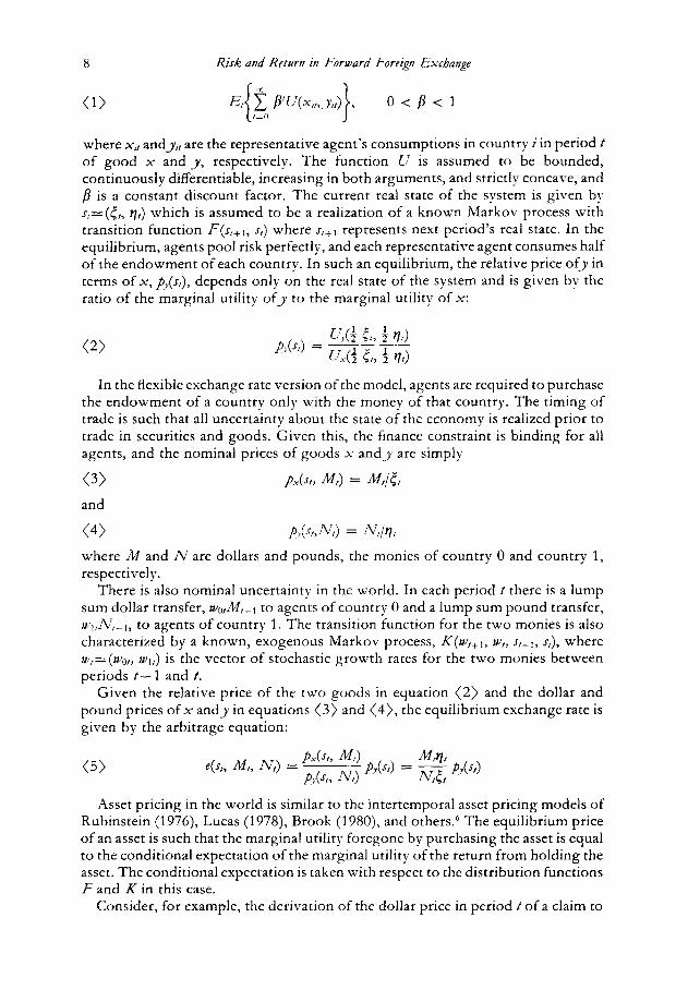
(1) Et 2 b’Wx,,,_y,t) , 0<8<1 I=0

where x,, andy;, are the representative agent’s consumptions in country i in period f of good x and J, respectively. The function U is assumed to be bounded, continuously differentiable, increasing in both arguments, and strictly concave, and b is a constant discount factor. The current real state of the system is given by s,=(<,, q,) which is assumed to be a realization of a known Markov process with transition function F(s,+i, s,) where I,+~ represents next period’s real state. In the equilibrium, agents pool risk perfectly, and each representative agent consumes half of the endowment of each country. In such an equilibrium, the relative price ofy in terms of x, p,(.r,), depends only on the real state of the system and is given by the ratio of the marginal utility ofy to the marginal utility of x:

(2)

In the flexible exchange rate version of the model, agents are required to purchase the endowment of a country only with the money of that country. The timing of trade is such that all uncertainty about the state of the economy is realized prior to trade in securities and goods. Given this, the finance constraint is binding for all agents, and the nominal prices of goods x andy are simply

(3)

and

(4)

where M and N are dollars and pounds, the monies of country 0 and country 1, respectively.

There is also nominal uncertainty in the world. In each period t there is a lump sum dollar transfer, wo,M,_, to agents of country 0 and a lump sum pound transfer, w,,N,_], to agents of country 1. The transition function for the two monies is also characterized by a known, exogenous Markov process, K(w,+i, w,, .r,+l, s,), where w,=(w,,,, w,,) is the vector of stochastic growth rates for the two monies between periods t- 1 and t.

Given the relative price of the two goods in equation (2) and the dollar and pound prices of x andy in equations (3) and (4), the equilibrium exchange rate is given by the arbitrage equation:

(5) 4-c, M,, N,) = P&t, M) P,(~,, N,) ph’) = $$f PYb)

Asset pricing in the world is similar to the intertemporal asset pricing models of Rubinstein (1976), Lucas (1978), Brook (1980), and others.b The equilibrium price of an asset is such that the marginal utility foregone by purchasing the asset is equal to the conditional expectation of the marginal utility of the return from holding the asset. The conditional expectation is taken with respect to the distribution functions F and K in this case.

Consider, for example, the derivation of the dollar price in period t of a claim to


one dollar with certainty in period t+ 1. Such a claim is equivalent to l/pX($,+l, M,+,)=M;’ (1 +%+l)- r,,, =$il units of x in period t+ 1 which is an uncertain amount that depends on the purchasing power of the dollar, x::,. The z;M+, units of x will be valued by agents in period t+ 1 at the marginal utility of x, U,(s,+,), which must be discounted back to period t by multiplication by the discount factor fi. The x-unit price of the claim to one dollar is therefore E,[pV,(s,+,)srf:,V,(s,)-‘1 which is obtained by taking the conditional expectation of the marginal value of the payoff on the asset and dividing by the marginal utility of x in period t since the opportunity cost of the investment is its x-unit price times the marginal utility of x in period t. The dollar price of the investment is then obtained by multiplication of the x-unit price byP,(s,,M,) or division by X, M. Therefore, the period t dollar price of a discount bill paying one dollar in period t+l is

(6)

Similarly, by replacing x withy in the above argument, , the period t pound price of a claim to one pound in the next period is found to be

(7)

where UJs,) is the marginal utility of_y in period t and n;Y is the purchasing power of the pound in terms ofy.

The discount bill prices in equations (6) and (7) are conditional expectations of the intertemporal marginal rates of substitution of dollars and pounds, respectively. Since these random variables are central to the discussion of risk in a monetary economy, we define them as

The intertemporal marginal rate of substitution of money is an index that weights the change in the purchasing power of the money by the intertemporal marginal rate of substitution of goods between the two periods. Since the exchange rate is the relative price of two monies, each of the rates of substitution is important in determining the risk premium in the forward foreign exchange market.

In order to determine the nature of the risk premium in the forward foreign exchange market, we must derive the forward price of foreign exchange, that is, the contract price set in period t at which one can buy and sell foreign exchange in period t+l.’ If there is no default risk on either nominal investment discussed above or on the forward contracts, investors must be indifferent between investing in the sure dollar denominated asset in which case the return is l/b.J~,,l~,) per dollar invested and the alternative covered interest arbitrage strategy of converting dollars into pounds, investing in sure pound denominated assets, and selling the proceeds in today’s forward market at pricef(~,,~,,M,,N,) of dollars per pound. The covered pound investment strategy yields [l/e(s,,M,,N,)] [l/&s,, w,)] If(s,,lv,,M,,N,)] per dollar invested. Equating the two investment strategies and substituting from above gives

10 Rid and Return in Forward Foreign Exchange

Taking the conditional expectation of next period’s exchange rate from equation (5) and subtracting equation (9) gives an expression for the risk premium in this

model:

Dividing both sides of equation (10) by e, normalizes the scale of the expression and provides an insight into the nature of the risk premium which depends upon the two currencies intertemporal marginal rates of substitution:*

Both real and monetary uncertainty enter the determination of the risk premium as well as the preferences of agents which act as weights in determining the importance of the fundamental sources of uncertainty represented by the real and monetary shocks to the two economies.

In order to develop an empirically testable hypothesis regarding the possibly time-varying risk premium in equation (1 l), Hansen and Hodrick (1983) exploited the fact that covered and uncovered investments in the pound-denominated riskless nominal return yield two dollar denominated returns that must satisfy the representation of the risk-return trade-off given by a conditional capital asset pricing model based on the conditional mean-variance frontier. That is, in equilibrium any dollar-denominated return, R,+,, must satisfy

(12) &(&,I - Rj+ ,) = P,E,( Rf, , - RX ,>

where /?,=C,(R,+I; Rf+,)/I,‘,(Rf+,), Rt,, is the dollar-denominated return on an appropriately chosen benchmark return on the conditional mean variance frontier,

and R:+,, is the return on an asset that is conditionally uncorrelated with the return on the benchmark asset.” When there exists a riskless nominal investment such as the one period bill described above, Rj,, can be chosen to be the nominal return

R f+, = 1 /b.&,,w,). Hansen, Richard, and Singleton (1982) establish that any return on the

conditional mean variance frontier is an appropriate benchmark return, and each of these returns satisfies:

(13) R:(+, = wR;+,+(l-w)R{+,

where R;,, is the minimum second moment return conditioned on the information set of agents, and O, is a possibly random weight that may depend on the conditioning set and which has the property that the probability of the event (w,=O) is zero. When markets are complete as m the Lucas model, one can think of agents having the opportunity to trade an asset with nominal return

(14) R;‘:, = Q;;I:,/C(Q;‘;,>’

and it is easily verified that this return is the minimum second moment return.“’ Now consider the dollar denominated returns mentioned above, covered and

uncovered investments in pounds. Each return must satisfy condition (12), and taking the difference of the two returns gives


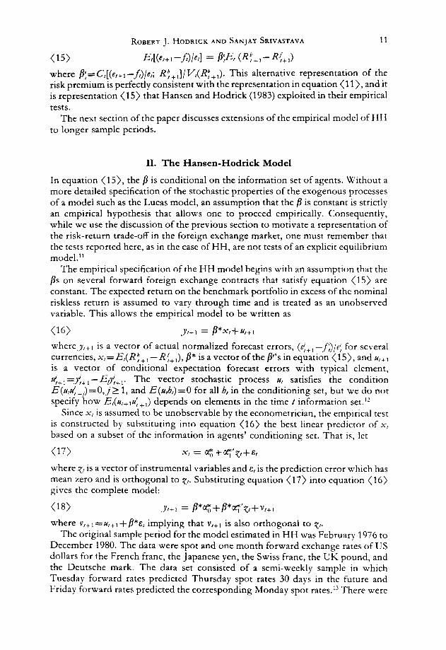
(15) E,[(e,+‘--f,)/e,l = B;E, (R:+,--{+,I

where &=C,[(e,+l-f/>/e,; R~+,]/Vt(R:+,). Th is alternative representation of the

risk premium is perfectly consistent with the representation in equation (1 I), and it is representation (15) that Hansen and Hodrick (1983) exploited in their empirical tests.

The next section of the paper discusses extensions of the empirical model of HH to longer sample periods.

II. The Hansen-Hodrick Model

In equation (1 S), the /I is conditional on the information set of agents. Without a more detailed specification of the stochastic properties of the exogenous processes of a model such as the Lucas model, an assumption that the fi is constant is strictly an empirical hypothesis that allows one to proceed empirically. Consequently, while we use the discussion of the previous section to motivate a representation of the risk-return trade-off in the foreign exchange market, one must remember that the tests reported here, as in the case of HH, are not tests of an explicit equilibrium model.”

The empirical specification of the HH model begins with an assumption that the fis on several forward foreign exchange contracts that satisfy equation (15) are constant. The expected return on the benchmark portfolio in excess of the nominal riskless return is assumed to vary through time and is treated as an unobserved variable. This allows the empirical model to be written as

(16) _Yt+1 = P*xt+~t+,

where-y,,’ is a vector of actual normalized forecast errors, (<+,-f;)/e; for several currencies, x,= E,(Rf+, - R$+,), #I * is a vector of the p’s in equation (15)) and tl,+, is a vector of conditional expectation forecast errors with typical element,

u’,+,=A+1-~&,. The vector stochastic process u, satisfies the condition E(u,ui_,)=O,j2 1, and E(ub,)=O f or all h, in the conditioning set, but we do not specify how E,(u,+,u: +, ) depends on elements in the time t information set.12

Since x, is assumed to be unobservable by the econometrician, the empirical test is constructed by substituting into equation (16) the best linear predictor of x, based on a subset of the information in agents’ conditioning set. That is, let

(17) XI = $+q’Q+c,

where i, is a vector of instrumental variables and E, is the prediction error which has mean zero and is orthogonal to 7,. Substituting equation (17) into equation (16) gives the complete model:

(18) J/+1 = B*q+p*EyQ+v,+l

where v,+’ =u,+’ +/I*&, implying that v/+1 is also orthogonal to 7,. The original sample period for the model estimated in HH was February 1976 to

December 1980. The data were spot and one month forward exchange rates of US dollars for the French franc, the Japanese yen, the Swiss franc, the UK pound, and the Deutsche mark. The data set consisted of a semi-weekly sample in which Tuesday forward rates predicted Thursday spot rates 30 days in the future and Friday forward rates predicted the corresponding Monday spot rates.‘” There were

12 Risk ond Return in Forward Foreign Exchange

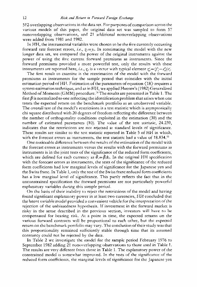
512 overlapping observations in the data set. For purposes of comparison across the various models of this paper, the original data set was sampled to form 57 nonoverlapping observations, and 21 additional nonoverlapping observations were added from 1981 and 1982.

In HH, the instrumental variables were chosen to be the five currently occurring forward rate forecast errors, i.e., Q=J,. In reestimating the model with the new longer data set, we compared the power of the original instruments against the power of using the five current forward premiums as instruments. Since the forward premiums provided a more powerful test, only the results with these instruments are reported here, i.e., x, is a vector with typical element z$=v,-e;)/t$

The first result to examine is the reestimation of the model with the forward premiums as instruments for the sample period that coincides with the initial estimation period of HH. Estimation of the parameters of equation (18) requires a system estimation technique, and as in HH, we applied Hansen’s (1982) Generalized Method of Moments (GMM) procedure.14 The results are presented in Table 1. The first p is normalized to one reflecting the identification problem that arises when one treats the expected return on the benchmark portfolio as an unobserved variable. The overall test of the model’s restrictions is a test statistic which is asymptotically chi-square distributed with 20 degrees of freedom reflecting the difference between the number of orthogonality conditions exploited in the estimation (30) and the number of estimated parameters (10). The value of the test statistic, 24.239, indicates that the restrictions are not rejected at standard levels of significance. These results are similar to the test statistic reported in Table 5 of HH in which, with the forecast errors as instruments, the test statistic had a value of 18.834.15

One noticeable difference between the results of the estimation of the model with the forecast errors as instruments versus the results with the forward premiums as instruments is in the joint tests of the significance of the reduced form coefficients, which are defined for each currency as e,==b,ai. In the original HH specification with the forecast errors as instruments, the tests of the significance of the reduced form coefficients had low marginal levels of significance for the Japanese yen and the Swiss franc. In Table 1, only the test of the Swiss franc reduced form coefficients has a low marginal level of significance. This partly reflects the fact that in the unconstrained specification the forward premiums are not particularly powerful explanatory variables during this sample period.

On the basis of their inability to reject the restrictions of the model and having found significant explanatory power in at least two currencies, HH concluded that the latent variable model provided a convenient vehicle for the interpretation of the rejection of the unbiasedness hypothesis. If investment in the forward market is risky in the sense described in the previous section, investors will have to be compensated for bearing risk. At a point in time, the expected returns on the various forward contracts will be proportional to each other, but the expected return on the benchmark portfolio may vary. The conclusion of their study was that this proportionality remained sufficiently stable through time that its assumed constancy could not be rejected by the data.

In Table 2 we investigate the model for the sample period February 1976 to September 1982 adding 21 nonoverlapping observations to those used in Table 1. The results are very different from those in Table 1. The explanatory power of the constrained model is somewhat improved. In the tests of the significance of the reduced form coefficients, the marginal levels of significance for the Japanese yen

TA

BL

E 1

. H

anse

n-H

odri

ck

late

nt

vari

able

m

odel

*

Y,+

I =

P*a,

*+D

*ar’

p,+

v,+

l

Cur

renc

y

Red

uced

fo

rm

coef

fici

ents

x2 5

) B

iI

All

i/‘s

(Std

. er

ror)

(S

td.

erro

r)

(Std

. er

ror)

(S

td.

erro

r)

(Std

. er

ror)

(S

td.

erro

r)

j>

1 =O

(S

td.

erro

r)

Con

fide

nce

Con

fide

nce

Con

fide

nce

Con

fide

nce

Con

fide

nce

Con

fide

nce

Con

fide

nce

R2

kr

1.

Fren

ch

fran

c

2.

Japa

nese

ye

n

3.

Swis

s fr

anc

4.

UK

po

und

5.

Deu

tsch

e m

ark

1.0

1.59

2 (0

.711

)

3.15

2 (0

.664

)

1.68

3 (0

.664

)

0.72

1 (0

.424

)

4.91

6 -0

.809

-

0.02

2 -1

.441

0.

837

(3.7

54)

(0.4

93)

(0.4

29)

(1.0

12)

(0.5

02)

0.81

0 0.

899

0.04

0 0.

845

0.90

5

7.82

8 -

1.28

9 -0

.035

-

2.29

4 1.

333

(6.8

72)

(0.6

38)

(0.6

79)

(1.7

97)

(0.7

19)

0.74

5 0.

957

0.04

1 0.

798

0.93

6

15.4

98

-2.5

51

-0.0

68

-4.5

41

2.63

9 (9

.957

) (1

.070

) (1

.352

) (2

.519

) (1

.060

) 0.

880

0.98

3 0.

040

0.92

9 0.

987

8.27

5 -1

.362

-0

.037

-

2.42

5 1.

409

(5.1

84)

(0.8

35)

(0.7

27)

(1.3

77)

(0.8

04)

0.88

9 0.

897

0.04

0 0.

922

0.92

1

3.54

4 -0

.583

-0

.016

-

1.03

8 0.

604

(3.9

93)

(0.5

79)

(0.3

10)

(1.0

74)

(0.6

23)

0.62

5 0.

686

0.04

0 0.

666

0.66

7

Tes

t of

the

con

stra

ined

m

odel

: x2

(20)

=24

.239

; co

nfid

ence

=0.7

68

2.24

4 (1

.425

) 0.

885

3.57

4 (2

.241

) 0.

889

7.07

6 (3

.075

) 0.

978

3.77

8 (2

.035

) 0.

937

1.61

8 (1

.611

) 0.

685

4.52

9 0.

524

5.27

0 0.

616

27.5

03

0.99

9

8.29

6 0.

859

1.25

3 0.

060

zi

0.15

4 : 3 v,

0.

000

E s s

0.03

0 3

Not

e:

The

de

pend

ent

vari

able

s ar

e th

e fo

rwar

d ra

te

fore

cast

er

rors

A+,

=

(p’+

, -x)

/e:,

US

dolla

rs

for

the

Fren

ch

fran

c,

the

Japa

nese

ye

n,

the

Swis

s

fran

c,

the

UK

po

und,

an

d th

e D

euts

che

mar

k.

The

in

stru

men

tal

vari

able

s ar

e th

e fo

rwar

d pr

emia

fo

r th

e sa

me

five

cur

renc

ies.

C

onfi

denc

e is

1 m

inus

the

mar

gina

l le

vel

of

sign

ific

ance

. V

alue

s of

th

e co

nfid

ence

te

rm

clos

e to

1

indi

cate

ev

iden

ce

agai

nst

the

null

hypo

thes

is

that

on

e or

a

set

of

coef

fici

ents

eq

uals

ze

ro.

All

fore

cast

er

rors

an

d fo

rwar

d pr

emia

ar

e ex

pres

sed

in

perc

ent

at

an

annu

al

rate

.

* Sa

mpl

e pe

riod

: Fe

brua

ry

1376

to

D

ecem

ber

1980

; nu

mbe

r of

ob

serv

atio

ns:

57.

TABLE

2.

Han

sen-

Hod

rick

la

tent

va

riab

le

mod

el*

.Y,+

I =

P*

a;:+

B*a

:‘a,

+v,

+t

Red

uced

fo

rm

para

met

ers

8,

&I

e 12

L

4 ,3 B

B

x2

5)

r4

IS

B

A

ll g’

s

PI

(Std

. er

ror)

(S

td.

erro

r)

(Std

. er

ror)

(S

td.

erro

r)

(Std

. er

ror)

(S

td.

erro

r)

j>l=

O

FQ

Cur

renc

y (S

td.

erro

r)

Con

fide

nce

Con

fide

nce

Con

fide

nce

Con

fide

nce

Con

fide

nce

Con

fide

nce

Con

fide

nce

R2

2 B

a

1.

Fren

ch

fran

c 5.

972

0.69

1 0.

034

? 9

2.

Japa

nese

ye

n

13.1

98

1 .o

(6.1

64)

0.96

8

2.05

9 27

.181

(0.8

00)

(9.0

52)

0.99

7

-0.0

80

- 1.

244

(0.2

06)

(0.7

41)

0.30

2 0.

907

-0.1

64

-2.5

62

(0.4

19

(1.1

13)

0.30

4 0.

979

- 0.

208

- 3.

243

(0.5

24)

(1.4

09)

0.30

8 0.

979

-0.0

98

- 1.

526

(0.2

45)

(0.8

60)

0.31

0 0.

924

- 0.

094

- 1.

472

(0.2

43)

(0.8

68)

0.30

2 0.

910

- 4.

467

(1.9

45)

0.97

8

-9.1

99

(2.6

14)

0.99

9

0.45

0 6.

080

(0.4

69)

(2.7

19)

0.66

3 0.

975

0.92

7 12

.521

(0.8

70)

(3.5

67)

0.71

3 0.

999

19.9

98

0.99

9

3.

Swis

s fr

anc

2.60

7 34

.411

(0.6

98)

(11.

473)

0.

997

1.22

7 16

.188

4.

U

K

poun

d (0

.373

) (7

.753

) 0.

963

(i:$

&

15.6

22

5.

Deu

tsch

e m

ark

(7.5

82)

0.96

1

-11.

646

1.17

3 15

.852

(3.0

66)

(1.1

14)

(4.1

38)

0.99

9 0.

707

0.99

9

- 5.

478

0.55

2 7.

457

(2.2

05)

(0.5

79)

(2.9

54)

0.98

7 0.

659

0.98

8

- 5.

287

0.53

3 7.

196

(2.2

68)

(0.5

62)

(3.1

30)

0.98

0 0.

657

0.97

9

22.9

10

0.99

9

7.25

8 0.

798

6.22

2 0.

715

0.02

4

Tes

t of

th

e co

nstr

aine

d m

odel

: x2

(20)

=34

.497

; co

nfid

ence

=0.9

77

Not

e:

see

Tab

le

1.

* Sa

mpl

e pe

riod

: Fe

brua

ry

1976

to

Se

ptem

ber

1982

; nu

mbe

r of

obs

erva

tions

: 78

.


and the Swiss franc are now very small. In contrast to Table 1, though, the chi-square test of the constrained model has a value of 34.497, which indicates that the restrictions of the model are rejected at all marginal levels of significance greater than 0.023. If the source of the rejection of the unbiasedness hypothesis is a time-varying risk premium, it appears that the assumptions of the HH model are too strong. Either the p’s in (15) are not constant, or some other model of risk and return is necessary to describe the risk premium.

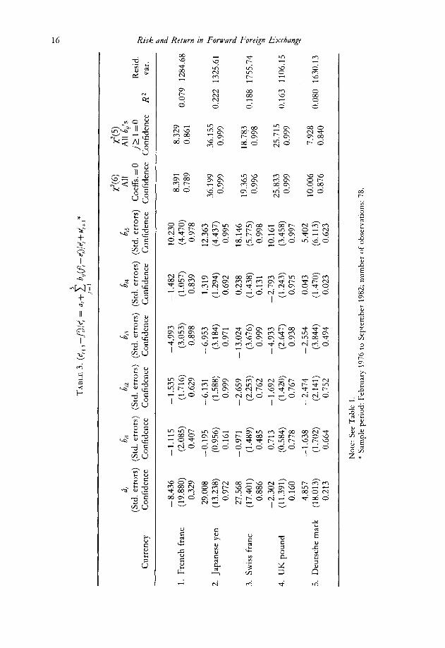
It is interesting to compare the results of Table 2 with the estimation of the unconstrained model presented in Table 3. These are ordinary least squares (OLS) estimates of the unconstrained reduced form coefhcients.16 Note the differences between the two sets of estimates. In the OLS regressions the coefficients of the instrumental variables that have weak explanatory power do not always have the same algebraic sign across currencies. This is true in the case of the constant terms and the coefficients of the forward premiums of the French franc and the UK pound although in none of the cases is the set of parameters particularly precisely estimated. Also, in the case of the coefficients which do have strong explanatory power in the unconstrained model, that is the coefficients of the Swiss franc and Deutsche mark forward premiums, the rank ordering across currencies is striking, but the proportionality is not of the same order of magnitude in each case. Finally, the imposition of the constraints causes a relatively severe loss in explanatory power as measured by the R2 for the French franc, the UK pound, and the Deutsche mark.

Given the rejection of the model of risk and return postulated in this section, it is important to reiterate that the model was a statistical hypothesis and not a precisely stated theory. Ideally, we would like to test a representation of dynamic equilibrium such as that set forth by Lucas and discussed in the previous section. Currently, the demands on the data to test such a model make it an exceedingly difficult task. For now, we set that task aside in order to investigate the stability of the reduced form coefficients presented in Table 3. This is done in the next section of the paper.

III. Parameter Stability

In this section, we investigate whether the rejection of the constraints in the HH model, documented in the previous section, is due to time-varying parameters and if so, why this might arise.

The theoretical analysis of Section I only postulates the existence of a trade-off between risk and return at a point in time, as in equations (12) and (15). It does not impose the restriction that the conditional covariance between the return on an asset and the return on the benchmark portfolio is constant or that the conditional variance of the benchmark portfolio is constant.

We shall work with the unconstrained model, estimated in Table 3. The reason is that even though the latent variable model is rejected relative to the unconstrained model, the cross-equation constraints may still be valid at any point in time as argued above, but the coefficients of the unconstrained model may not be constant through time. Alternatively, the coefficients of the unconstrained model could be constant and the restrictions of the HH model not hold under alternative hypotheses regarding the nature of risk and return in the forward foreign exchange market. This motivates our investigation of the stability of the coefficients of the unconstrained model.

Cur

renc

y

&,

62

x2(6

) x2

(5)

1 4 6^

tJ

64

65

All

All

t$‘s

(S

td.

erro

rs)

(Std

. er

rors

) (S

td.

erro

rs)

(Std

. er

rors

) (S

td.

erro

rs)

(Std

. er

rors

) C

oeff

s.=O

,j>

l=O

C

onfi

denc

e C

onfi

denc

e C

onfi

denc

e C

onfi

denc

e C

onfi

denc

e C

onfi

denc

e C

onfi

denc

e C

onfi

denc

e R

2 R

esid

. h

var.

2 h

1.

Fren

ch

fran

c -

8.43

6 -1

.115

(1

9.88

0)

(2.0

85)

0.32

9 0.

407

29.0

08

-0.1

95

2.

Japa

nese

ye

n (1

3.23

8)

(0.9

56)

0.97

2 0.

161

27.5

68

-0.9

71

3.

Swis

s fr

anc

(17.

401)

(1

.489

) 0.

886

0.48

5

-2.3

02

0.71

3

4.

UK

po

und

(11.

391)

(0

.584

) 0.

160

0.77

8

4.85

7 -

1.63

8

5.

Deu

tsch

e m

ark

(18.

013)

(1

.702

) 0.

213

0.66

4

-1.5

35

(1.7

16)

0.62

9

-6.1

31

(1.5

88)

0.99

9

- 2.

659

(2.2

53)

0.76

2

- 1.

692

(1.4

20)

0.76

7

- 2.

474

(2.1

41)

0.75

2

-4.9

93

- 1.

482

(3.0

53)

(1.0

57)

0.89

8 0.

839

- 6.

953

(3.1

84)

0.97

1

- 13

.024

(3

.676

) 0.

999

-4.9

33

(2.6

47)

0.93

8

-2.5

54

(3.8

44)

0.49

4

1.31

9 (1

.294

) 0.

692

0.23

8 (1

.438

) 0.

131

- 2.

793

(1.2

43)

0.97

5

0.04

3 (1

.470

) 0.

023

10.2

30

(4.4

70)

0.97

8

12.3

63

(4.4

37)

0.99

5

18.1

46

(5.7

75)

0.99

8

10.1

61

(3.4

58)

0.99

7

5.40

2 (6

.113

) 0.

623

8.39

1 8.

329

0.78

9 0.

861

36.1

99

36.1

55

0.99

9 0.

999

19.3

65

18.7

83

0.99

6 0.

998

25.8

33

25.7

15

0.99

9 0.

999

10.0

06

7.92

8 0.

876

0.84

0

0.07

9 12

84.6

8 $ * a 3,

0.22

2 13

25.6

1 2 2 9 Q

L

0.18

8 17

55.7

4 ? 4’

0.16

3 11

06.1

5 ? 5 2 %

?

0.08

0 16

30.1

3

Not

e:

See

Tab

le

1.

* Sa

mpl

e pe

riod

: Fe

brua

ry

1976

to

Se

ptem

ber

1982

; nu

mbe

r of

ob

serv

atio

ns:

78.


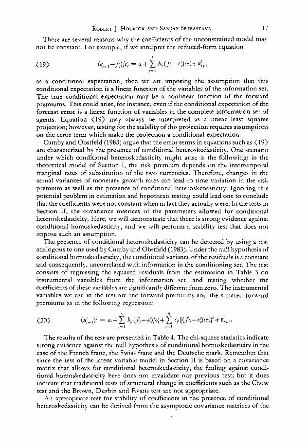
There are several reasons why the coefficients of the unconstrained model may not be constant. For example, if we interpret the reduced-form equation

(19) (ei,+,-x)/e: = ~,+t b,Cf:--e:)le:+u’+, /=1

as a conditional expectation, then we are imposing the assumption that this conditional expectation is a linear function of the variables of the information set. The true conditional expectation may be a nonlinear function of the forward premiums. This could arise, for instance, even if the conditional expectation of the forecast error is a linear function of variables in the complete information set of

agents. Equation (19) may always be interpreted as a linear least squares projection; however, testing for the stability of this projection requires assumptions on the error term which make the projection a conditional expectation.

Cumby and Obstfeld (1983) argue that the error terms in equations such as (19) are characterized by the presence of conditional heteroskedasticity. One scenario under which conditional heteroskedasticity might arise is the following: in the theoretical model of Section I, the risk premium depends on the intertemporal marginal rates of substitution of the two currencies. Therefore, changes in the actual variances of monetary growth rates can lead to time variation in the risk premium as well as the presence of conditional heteroskedasticity. Ignoring this potential problem in estimation and hypothesis testing could lead one to conclude that the coefficients were not constant when in fact they actually were. In the tests in Section II, the covariance matrices of the parameters allowed for conditional heteroskedasticity,. Here, we will demonstrate that there is strong evidence against conditional homoskedasticity, and we will perform a stability test that does not impose such an assumption.

The presence of conditional heteroskedasticity can be detected by using a test analogous to one used by Cumby and Obstfeld (1983). Under the null hypothesis of conditional homoskedasticity, the conditional variance of the residuals is a constant and consequently, uncorrelated with information in the conditioning set. The test consists of regressing the squared residuals from the estimation in Table 3 on instrumental variables from the information set, and testing whether the coefficients of these variables are significantly different from zero. The instrumental variables we use in the test are the forward premiums and the squared forward premiums as in the following regression:

(20)

The results of the test are presented in Table 4. The chi-square statistics indicate strong evidence against the null hypothesis of conditional homoskedasticity in the case of the French franc, the Swiss franc and the Deutsche mark. Remember that since the test of the latent variable model in Section II is based on a covariance matrix that allows for conditional heteroskedasticity, the finding against conditional homoskedasticity here does not invalidate our previous test; but it does indicate that traditional tests of structural change in coefficients such as the Chow test and the Brown, Durbin and Evans test are not appropriate.

An appropriate test for stability of coefficients in the presence of conditional heteroskedasticity can be derived from the asymptotic covariance matrices of the


TABLE 4. Test for conditional homoskedasticity: equation (20)*

Test statistic Currency x2(10)6, = c,, = 0 VJ Confidence

1. French franc 32.559 0.999 2. Japanese yen 14.485 0.848 3. Swiss franc 96.655 0.999 4. UK pound 10.557 0.607 5. Deutsche mark 26.038 0.996

* Sample: February 1976 to September 1982; number of

observations: 78.

coefficients estimated over two sample periods. Hansen (1982) and Cumby, Huizinga, and Obstfeld (1983) d escribe procedures for estimation which do not require the traditional assumptions of strict exogeneity of the regressors and conditional homoskedasticity of the error term. These procedures were followed in the estimation of the constrained and unconstrained models of Section II and are described briefly in the Appendix. Our test is appropriate given their regularity conditions.

In the unconstrained model, the GMM estimator for a sample of size T, is strongly consistent and asymptotically normally distributed. That is,

(21) dm-B*, - N(O, Q)

where b, is the GMM estimate of /?*, which reduces to the OLS estimate in this case, and n,=c;‘s,X;‘, where the covariance matrix, a,, is constructed from the following sample moments:

(22) and

where 2; is the vector of instruments and tr’,,, is the corresponding error term for the equation. Under the maintained hypothesis of no serial correlation in the error process, and under the null hypothesis that /?I=/&, the test statistic

(23) $1 -/ja)‘Q-’ <A - B2)

has an asymptotic chi-square distribution with m degrees of freedom, where m is the dimension of a*, b I and 82 are the estimates of /3* over the two subsamples, and fi=(Q,/T, +Q/Tr).” Th e results are presented in Table 5.

We performed three sets of tests. The first test examines the HH conjecture that the observations from the transitional years of the flexible exchange rate period from July 1973 when our data series begin until the formal ratification of the

ROBERT J. HODRICK AND SANJAY SRIVASTAVA

TABLE 5. Tests for constant coefficients

19

Currency Test

statistic Confidence

JM~ 1973 to January 1976and February 1976 to December

1980


Februar_y 1976 to December 1980 and januaq 1981 to

September 1982

1. French franc 7.101 0688 2. Japanese yen 4.900 0.443 3. Swiss franc 5.501 0.518 4. UK pound 10.996 0.911 5. Deutsche mark 10.942 0.909

February 1976 to October 1979 and November 1979 to

September 1982


Rambouillet agreement in January 1976 should be omitted. The ratification amended the Articles of Agreement of the International Monetary Fund to allow countries to adopt a flexible exchange rate as their dejure system. We performed the tests between the periods July 1973 to January 1976 and February 1976 to December 1980. The latter is the sample period employed by HH. The tests indicate strong evidence against the null hypothesis of constant coefficients for the case of the Japanese yen, the Swiss franc, and the UK pound.

The second tests examines the hypothesis that the coefficients of the unconstrained model did not differ significantly when the 21 additional observations were added to the HH sample. The results from these tests provide some evidence against the null hypothesis for the UK pound and the Deutsche mark. It is interesting to note that there is no strong evidence against the null hypothesis for the two currencies for which we obtained the most explanatory power in the constrained model, namely the Japanese yen and the Swiss franc.

The third test compared the estimated coefficients before and after the Carter intervention in October 1979 and the resulting change in Federal Reserve Board operating procedures. The two samples were February 1976 to October 1979 and November 1979 to September 1982. This appeared to be a natural point at which to perform the test given the change in US policy. Somewhat surprisingly, we found evidence against the null hypothesis only in the case of the French franc and the UK pound. The yen and the Swiss franc tests again demonstrate no evidence against structural change.


We turn next to the interpretation of these tests. There is some evidence against the hypothesis of no structural change. Given only this evidence, though, one might conclude that the linear model with constant coefficients was a good approximation of the true conditional expectation. However, there is additional strong evidence that the conditional expectations of the forecast errors are nonlinear functions of the forward premiums. In particular, if we also include squared forward premiums as right-hand side variables in equation (19), we find that the coefficients on these additional terms are highly significant. The results of the estimation are presented in Table 6.

TABLE 6.(<+, --x)/e; = u,+,g byV:-P:)i$+,$ ~i/[Cf:-eW!12+~:+,*

Currency X’(5) 6,,=0j=1,5 X2(5) C,,=0J=1,5 X2(10) b,=&,=Oj=1,5

Confidence Confidence Confidence

1. Prench franc 19.171 21.741 26.951 0.998 0.999 0.997

2. Japanese 9.029 9.753 44.527 yen

0.892 0.917 0.999

3. Swiss franc 22.782 23.163 59.059 0.999 0.999 0.999

4. UK pound 8.578 10.900 68.693 0.873 0.947 0.999

5. Deutsche mark 13.119 13.292 23.633 0.978 0.979 0.991

* Sample: February 1976 m September 1982; number of observations: 78.

Nonlinearity of the conditional expectation could be responsible for the evidence against time-invariant parameters and also for the evidence against conditional homoskedasticit!;. Some evidence for this interpretation is provided by the fact that when the squared forward premiums are added as additional instruments to the specification in (l9), we cannot reject time-invariance of the coefficients. The results of this last test are given in Table 7.‘*

The nonlinearity of the conditional expectation of the forecast error in the forward premiums is inconsistent with the assumed constancy of the betas in the HH model which is the likely reason for its rejection. Since the tests of this section provide strong evidence only against the unbiasedness hypothesis without providing a truly convincing model of the risk premium, we turn in the next section to an examination of speculative trading strategies based on equations like (19).

IV. Speculative Profits

In this section, we examine Bilson’s (1981) contention that the risk-return trade-off from speculating in forward currency markets is too favourable to be consistent

with risk averse behavior.


TABLE 7.

Currency Test statistic

x2 (11) Confidence


* Period: February 1976 to October 1979 and November 1979 to September 1982.

His strategy is to forecast spot exchange rates with a model analogous to that represented by equation (19).‘” Using the covariance matrix of the error terms in the equations, he forms a portfolio of positions in the forward market to minimize the variance of the portfolio subject to an expected profit constraint. Denoting by 8, the estimated covariance matrix of the error terms in the equations, the portfolio weights in period t, q,, are chosen as follows:

(24) min q: O,q, subject to q:r, = 7~* N

where r, is the vector of expected forecast errors and rc* is the desired profit. The

solution to the problem in (24) is

(25) @ = 0;’ r,(ri 0;’ r,)-‘rr*

where the variance of the portfolio is given by

(26) 0; = qy et@ Note thal this model implies a linear portfolio efficient frontier in each period and

presumes that the investor cares only about the first two moments of his forward market portfolio, and not about its covariation with other asset returns or his consumption stream, as would be implied by the Lucas model of Section I.

The basis of Bilson’s position is an examination of standardized expected profits (SRE) which are defined to be expected profits divided by the standard deviation of the portfolio and standardized actual profits (SRA) which are analogously defined using actual profits. In his research, an equation like (19) was estimated using a basket of nine currencies for the sample period July 1974 to January 1980.20 The estimated parameters were used to form expected profits which were combined with the estimated covariance matrix to construct portfolios as in equation (25). The out-of-sample profitability of following this strategy for one year was computed. His estimates yielded an average SRE of 0.929, and an average SRA of 0.857. Applying a two-standard deviation rule, this implies that expected profits are one and the two-sigma band runs from - 1.153 to 3.153, which forms the basis for his contention.

The result that average SRE is approximately one is indeed striking andprima

22 Risk and Refurn in Forward Foreign Exchange

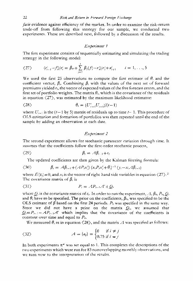
facie evidence against efficiency of the market. In order to examine the risk-return trade-off from following this strategy for our sample, we conducted two experiments. These are described next, followed by a discussion of the results.

Experiment 1

The first experiment consists of sequentially estimating and simulating the trading strategy in the following model:

(27) (e:,, -f:)/e; = P,o+ i PYCf:-e:)/e:+t/:+, i= 1,...,5 ,=I

We used the first 25 observations to compute the first estimate of 8, and the coefficient vector, p,. Combining B, with the values of the next set of forward premiums yielded r,, the vector of expected values of the five forecast errors, and the first set of portfolio weights. The matrix 8,, which is the covariance of the residuals in equation (27), was estimated by the maximum likelihood estimator:

(28) 6 = (~:_,~,_,)/(t-l)

where U,_, is the (t- 1 by 5) matrix of residuals up to time t- 1. This procedure of OLS estimation and formation of portfolios was then repeated until the end of the sample by adding an observation at each date.

Experiment 2

The second experiment allows for stochastic parameter variation through time. It assumes that the coefficients follow the first-order stochastic process,

(29) P, = (~Pt-,+s!

The updated coefficients are then given by the Kalman filtering formula:

(30) D, = nj3-,+(AP~;) (x,P,X:+e,)-’ (v,-A?@-1)

where E(s,)=O, and x, is the vector of right-hand side variables in equation (27).” The covariance matrix of /?, is

(31) P, = AP,_,A’+Q,

whereQ, is the covariance matrix of&,. In order to run the experiment, _-1, PO, Po,Q, and 8, have to be specified. The prior on the coefficients, PO, was specified to be the OLS estimate of p based on the first 24 periods. PO was specified in the same way. Since we did not have a prior on the matrix Q,, we assumed that

Q,=P,_,-AAP,_,A’ which implies that the covariance of the coefficients is constant over time and equal to PO.

Vi’e measured 0, as in equation (28), and the matrix A was specified as follows:

(32) A = {a,} = 0 ifi #I

0.75 if i = j

In both experiments II* was set equal to 1. This completes the descriptions of the two experiments which were run for 83 nonoverlapping monthly observations, and we turn now to the interpretation of the results.


The results of the first experiment show that over the sample, average SRE was 0.871 and average SRA was 0.211. The values of SRE ranged between 0.255 and

2.516. It is possible to test if profits at time t are drawn from a normal distribution with

mean II* and variance a:. Let 6; denote the estimated portfolio variance at t. Assuming that the distribution of profits is normal, standardized unexpected profit, (rr,-n*)/b,, has a t-distribution with (t-6) degrees of freedom. Hence, by Liapunov’s Central Limit Theorem, the statistic

(33)

f (71,~7tn*)/cf, t=t,,

[ e (t-b)/(t-8) : I=,,, 1

has an asymptotic standard normal distribution where to=26 and T=108 which are the 83 observations for the experiments. 22 We tested whether r~, was significantly different from one and zero. For the null hypothesis x*=0, the test statistic was 1.883 which corresponds to a marginal level of significance of 0.060. For the null hypothesis n *= 1, the test statistic was - 5.889 which corresponds to a marginal level of significance smaller than 0.001. Both the null hypotheses are rejected by the data, the latter more strongly than the former.

The results of the second experiment show that over the sample, average SRE was 0.660 and average SRA was 0.620. The values of SRE ranged between 0.061 and 4.573. Once again, we tested whether n, was significantly different from one and zero. For the null hypothesis n*=O, the test statistic was 5.536 which corresponds to a marginal level of significance smaller than 0.001. For the null hypothesis 5~* = 1, the test statistic was -0.358 which corresponds to a marginal level of significance of 0.72. In this case, we cannot reject the hypothesis that n*= 1, while the hypothesis that x*=0 is rejected.

In experiment 2, since we cannot reject II * = 1, it makes sense to examine the implied risk-return trade-off as measured by the mean and standard deviation of profits. Applying the two standard deviation rule, expected profits are one, and the two-sigma band runs from -2.030 to 4.030. This is a less favourable risk-return trade-off than that found by Bilson. Once again, this trade-off is based on the average SRE. When SRE was equal to 0.061, the implied two-sigma band was -31.787 to 33.787, and when SRE was equal to 4.573, the band ran from 0.563 to 1.437. The latter trade-off is extremely favorable, while the former is highly unfavorable. It is not obvious how seriously one should take these extreme values since they depend on the estimated values of the parameters. Nevertheless, it would appear from the volatility of the risk-return trade-offs at different points in time that a speculator in foreign exchange must be willing to bear a considerable amount of risk, even if risk is measured in the way described above, ignoring consumption risk, etc.

V. Conclusions

The analysis conducted in the paper was motivated by an attempt to explain the now common rejection of the unbiasedness hypothesis. As was discussed in the introduction, various explanations have been offered for this finding. One

24 Risk and Return in Forward Fareign Exchange

explanation is based on the existence of a risk premium, and the analysis in this paper addressed the problem from this perspective.

There are strong empirical and theoretical reasons for believing a priori in the existence of a risk premium. For instance, Ibbotson and Sinquefield (1976) have documented the existence of large differences in the average holding period returns on a variety of assets. Most financial economists view these differences as reflecting risk premiums, and one would therefore expect to find a risk premium in the forward foreign exchange market especially given the modern approach to exchange rate determination, which argues that foreign exchange rates are determined in asset markets. In intertemporal asset pricing theory, the covariation between intertemporal marginal rates of substitution on monies and the nominal returns on assets induces a risk premium on an asset. In the Lucas model of Section I, the risk premium on a forward contract depends on the same covariation, since forward contracts are risky nominal assets.

Hansen and Hodrick (1983) p oint out the difficulties of testing the equilibrium model of Section I. As in that paper, we have not attempted to measure the intertemporal marginal rates of substitutions of currencies directly, nor have we attempted to specify an explicit equilibrium econometric study. Our goals have been more modest, yet we believe that the results presented here provide some insights into the workings of forward exchange markets.

We found that one reason for the rejection of the Hansen-Hodrick model is the assumed constancy of the p’s which is inconsistent with the observed nonlinearity of the conditional expectations of the forecast errors in the forward premiums. We observed that this could also be responsible for the presence of heteroskedasticity reported by Cumby and Obstfeld (1983).

In the introduction, we noted that since much of our work is of necessity based on asymptotic distribution theory, proponents of the unbiasedness hypothesis will probably remain skeptical about the rejection of the unbiasedness hypothesis which appears throughout this paper. Such a position is tenable, but as sample sizes have grown, the numerous rejections of the hypothesis which are now commonplace form a substantial body of evidence which is increasingly difficult to ignore.

With regard to the second position within the profession, which argues that the rejection of the unbiasedness hypothesis ought to be related to the outstanding stocks of government bonds, we note that the discussion of the Lucas model in Section I was independent of the existence of such assets. Nominal government bonds may be important determinants of the purchasing power of a currency, in which case we would expect them to have a role in the determination of a risk premium. However, the lack of significant explanatory power of such assets in an equation like (19) does not constitute evidence against the existence of a risk premium.

The last section of our paper investigates the claim that particular trading strategies in the forward foreign exchange market yield a risk-return trade-off which is too favorable to be accounted for by risk aversion, Upon conducting experiments based on the trading strategy of Bilson (1981), we found that the strategy was profitable, but it also required willingness on the part of the speculator to absorb a substantial variance of profits. The experiments were run over an eight-year period and produced statistically significant out-of-sample profits. This profitability is consistent either with the existence of a risk premium or with market inefficiency. In any case, it provides further evidence against the unbiasedness


hypothesis. The volatility of actual profits and the magnitude of average standardized profit suggest to us that a risk premium is the likely explanation.

Appendix

In this appendix, we describe the estimation of the parameters and their asymptotic covariance matrices for the two models discussed in the text. Estimation in both models is an example of the procedure referred to by Hansen (1982) as the Generalized Method of Moments (GMM). The estimation procedure is also described in Hansen and Singleton (1982) and in Hansen and Hodrick (1983).

The HH model is a system of five equations,

(34) Jr+1 = P*a0*+P*q’?j+vt+l

in ten parameters, 6’ = (/?*‘, c$, a?‘). We assume that the stochastic process p, is stationary and ergodic. The orthogonality conditions are

(35) ~,(Zk3Vt+1) = 0

which is a 30 element vector formed from the unobservable error term. Estimation proceeds by defining two functions of the observable data and the parameters to be estimated:

(36) fcJ,+1,~t,S) = ~,+l-p”~,*-P*q’?j)o~,

z MJt+,,?g)OQ

and by forming the moment estimator of the function,fCy,+i, Q,c?), for a sample of size T:

(37)

For large values of T,gT(8) ought to be close to zero if the model is true. Estimation of the parameters requires the choice of a weighting matrix W7, and the parameters are chosen to minimize the criterion function,

(38) _/7(d) = g7tcVw7g7tcV

Hansen (1982) describes the optimal choice of W7. It is optimal in the sense of minimizing the asymptotic covariance matrix of the parameters for the class of estimators that exploit the same orthogonality conditions.

The covariance matrix of the parameters is

(39) n(s) = (D;w,.D,.)-’

where

(40) Dr = f $ $ C_Y,+L zt, @OZt r-1

and

in this case since we assume v,+i to be mean zero and serially uncorrelated. We followed the suggestion in Hansen and Singleton (1982) of removing the sample means g7(8)97(b)’ from the cross-productsf(yl+I,Z,,S~~,+I,Zt,6)’ m computing WT. They note that this adjustment has no effect on the asymptotic properties of the estimates or the test statistics, yet under alternative hypothesesg7(b) may not be zero. The adustment improves the power of the test.

Hansen demonstrates that T times the value of the criterion function at its minimum is


asymptotically chi-square distributed with degrees of freedom equal to the number of orthogonality conditions minus the number ofestimated parameters. This is the test statistic for the model.

The estimation of the unconstrained model is a GMM procedure which reduces to equation by equation ordinary least squares. As in the above discussion, the derivation of the covariance matrix does not impose conditional homoskedasticity. The covariance matrix of the parameters for a particular equation has the same form as equation (39), but DT- reduces to (l/T)Z’Z where Z is the (Txk) matrix of instruments, and W7 reduces to

1.

2.

3. 4.

5.

6.

7.

8.

9

Notes

A large literature now exists on this topic. Major empirical contributions fo the area have been

made by Dooley and Shafer (1976, 1982), Frenkel (1977, 1981), Stockman (1978), Lerich (1978, 1979a), Geweke and Feige (1979). Frankel(l980,1982), H amen and Hodrick (1980,1983), Bilson (1981), Cumby and Obstfeld (1981, 1983). Hakkio (1981a, 1981b), Longworth (1981), and Hsieh

(1982).

hicKinnon (1979, p.156) has argued

that the supply of private capital for taking net posirions III either the forward or spot markets IS currently

madequare. Exchange rates can move sharply in response to random rar~anons m the day-to-day demands b!

merchants or from monetary disturbances. Once a rate starts to move because of some temporary perturbation, no prospective speculator is willing to hold an open position for a significant time interval in

order to bet on a reversal--whence the large daily and monthly morements I” the foreign exchanges and

sometimes high bid-ask spreads. Bandwagon psychologies result from the general unwillingness of

participants to take net positions against near-term market movements that are necessarily accentuated by the

behavior of nonspeculatnx merchants.

See Levich (1979b) for an analysis of commercial forecasting services. Michael Mussa made this criticism at the NBER Conference on Exchange Rates and International hlacroeconomics held in Cambridge, hlassachusetts in November 1981. I&asker (1980) argued

that the existence of a particular event such as a discrete devaluation could bias the sampling

distribution of the test statistics such that they are poorly approximated by their asymptotic

distribution under the null hypothesis. This parricular problem is not unique to studies of the

foreign exchange market because it plagues much of modern time series analysis. Korajczyk

(1983) has rejected the unbiasedness hypothesis using bootstrap methods to adjust for small

sample bias. This point is generally acknowledged by those who reject the unbiasedness hypothesis. The work

of, for example, Grauer, Litzenberger and Stehle (1976), Kouri (1977), Stockman (1978), Fama

and Farber (1979), Frankel (1979). Roll and Solnick (1979). Hodrick (1981), and St& (1981) provides theoretical models of a risk premium. These models also demonstrate that the expected

real rate differential between nominal riskless assets denominated in two different currencies is

exactly the same as the risk premium separating forward rates from expected future spot rates.

See Breeden (1979) and Grossman and Shiller (1982) for a discussion of the conversion of these models into ‘consumption beta’ models. Stulz (1981) generalized the Breeden approach to

consider pricing of international assets. Hansen and Singleton (1983) conduct econometric

analysis of the intertemporal models using aggregate consumption data.

A discussion of the determination of the forward foreign exchange rate and the risk premium that

separates it from the expected future spot rate was included in early drafts but excluded from the

published version of Lucas (1982). An alternative representation of the right-hand side of equation (11) is obtained by taking the

conditional expectation of the second order Taylor series expansion of @E,/Q~E,) around

E,cQ~~,) and E@f”,,). The resulting expression is

~dQ,M,,)-aQ,M,,; [l/~I~f:,)12{[~r~~,/~/~~,)l

a;“,,)} where V,(e) and C,( a;*) are the conditional variance and the

conditional covariance, respectively.

As demonstrated by Roll (1977) and extended to conditional environments by Hansen, Richard


and Singleton (1982), the content of the restriction embodied in equation (12) is that the

benchmark return is on the conditional mean-variance frontier. The static capital asset pricing

model is often given empirical content through the assumption by the econometrician that

measurements on an aggregate wealth portfolio are mean-variance efficient. As in HH, no such

assumption is made here. 10. Equation (14) follows immediately once one recognizes that all nominal dollar denominated

returns satisfy E,(R,+@;M,,)=l. 11. Singleton (1983) is relatively optimistic about the ability of econometricians to estimate directly

from equations such as equation (11) by using observations on aggregate consumption series and

price indexes. We are suspect of what one may gain from such an approach given the severe measurement error problems that are encountered in using macro time series although see Hansen

and Singleton (1983).

12. Cumbv and Obstfeld (1983) g ar ue that forward rate forecast errors are characterized by

conditional heteroskedasticity. Hence, we do not assume homoskedastic disturbances. This issue

is investigated in Section III.

13. Hakkio (1983) argues correctly that the forward rates are not matched precisely with the

appropriate value date one month in the future. Riehl and Rodriguez (1977) discuss the rules

which regulate the determination of the exact delivery day when the contract is to be executed.

Hsieh (1982) and Cumby and Obstfeld (1983) match the data precisely taking account of such

factors as holidays with no difference in inference regarding evidence against the unbiasedness

hypothesis. 14. See the Appendix for a discussion of the estimation procedure.

15. Using the forecast errors as instruments, sampling the HH data to form a data set of 57

observations, and reestimating the HH model gives a x2(20)=18.459. Hence, the sampling

procedure does not appear to have reduced the power of the test significantly.

16. Note that we allow for some forms of conditional heteroskedasticity in the construction of the

covariance matrix of the parameters. See the Appendix for details. Cumby and Obstfeld (1983)

and Hsieh (1982) argue for this approach, which was proposed by White (1980).

17. Note that this is an asymptotic test, and in theory, requires two infinitely large, disjoint samples.

18. Note that estimation of the HH model with eleven instruments and five currencies would impose

55 orthogonality conditions in the estimation. At this point, this is computationally impractical

which is why we did not attempt to reestimate the HH model with this specification.

19. We chose to use equation (19) rather than the specification in Table 7 for two reasons. First,

forecasting with a larger number of variables involves a tradeoff between an improvement in the

forecast due to these variables and a worsening of the forecast due to increased estimation error.

The inclusion of the squared and ‘cross-product’ terms adds 15 coefficients to those in equation

(19). 20. Bilson’s specification is

(e:,, -_/J/e: = a,[[(f:-~)/ea.'+a2[(f:-e:)/e:;',+u:+,

where superscript Sand L. refer to ‘small’ and ‘large’. Small forward premia are those less than 10 per cent in absolute value. He uses the five currencies of this study plus the Canadian dollar, the

Belgian franc, the Italian lira, and the Dutch guilder. The estimation imposes the constraint that

the coefficients are identical across currencies. Both studies ignore transactions costs, which

would reduce profitability. To make our study comparable to Bilson’s, we target a fixed level of profit in each period, regardless of the risk-return tradeoff. A risk-averse investor would not follow such a strategy.

21. See Schweppe (1973).

22. See Dhrymes (1974).

References

BILSON, J.F.O., ‘The “Speculative Efficiency” Hypothesis’,]. Business, July 1981, 54: 435-452. BREEDEN, D.T., ‘An Intertemporal Asset Pricing Model with Stochastic Consumption and

Investment Opportunities’,]. FinanciaI Econ., 1979, 7: 265-296.

BROCF, W.A., ‘Asset Pricing in an Economy with Production: “Selective” Survey of Recent Work on Asset-Pricing Models’, in Pan-Tai Lit-t, ed., Dynamic Optimi~afion and Mathematical Economics, New York: Alenum Press, 1980.

28 Ri_& and Return in Forward Foreign Exchange

CUMBY, R.E. AND M. OBSTFELD, ‘A Note on Exchange-Rate Expectations and Nominal Interest

Differentials: A Test of the Fisher Hypothesis’,]. Finance, June 1981, 36: 69?-704. CUMBY, R.E. AND M. OBSTFELD, ‘International Interest-Rate and Price-Level Linkages Under Flexible

Exchange Rates: A Review of Recent Evidence’, in J.F.O. Bilson and R.C. Marston, eds, Exchange Rates: Theoy and Practice. Chicago: University of Chicago Press for the NBER, 1983.

CUMBY, R.E., J. HUIZINGA AND M. OBSTFELD, ‘Two-Step Two-Stage Least Squares Estimation in Models with Rational Expectations’, /. Econometrirs, April 1983, 21: 333-355.

DOOLEY, M.P. AND J.R. SHAFER, ‘Analysis of Short-Run Exchange Rate Behavior: March, 1973 to

September, 1975’, International Finance Discussion Paper, No. 123, Federal Reserve Board,

Washington, 1976. DOO~EY, M.P. AND J.R. SHAFER, ‘Analysis of Short-Run Exchange Rate Behavior: March, 1973 to

November, 1981’. Forthcoming in D. Bigman and T. Taya, eds, Exchange Rate and Trade Instability: Causes, Consequences, and Remedies, Cambridge, Mass.: Ballinger, 1983.

DHRYMES, P. J., Econometrics: Statistical Foundations and Applications. New York: Springer-Verlag,

1974.

FAMA, E. AND A. FARBER, ‘Money, Bonds, and Foreign Exchange’, .4m. Econ. Rec., September 1979,

69: 269-282. FRANKEL, J.A., ‘The Diver&ability of Exchange Risk’, /. Int. Econ., August 1979, 9: 379-393.

FRANKEL, J.A., ‘Tests of Rational Expectations in the Forward Exchange Market’, South. Eron. J., April 1980,46: 1083-1101.

FRANKEL, J.A., ‘In Search of the Exchange Risk Premium: A Six-Currency Test Assuming Mean

Variance Optimization’,j. /nt. Monq and Finance, December 1982, 1: 2555274.

FRENKEL, J.A., ‘The Forward Exchange Rate, Expectations, and the Demand for Money: The

German Hyperinflation’, Am. Econ. Rev., September 1977, 67: 653-670. FRENKEL, J.A., ‘Flexible Exchange Rates, Prices, and the Role of ‘News’: Lessons from the 197Os’,J.

Pal. Econ., August 1981, 89: 655-705.

GEWEKE, J.F. AND E.L. FEIGE, ‘Some Joint Tests of the Efficiency of Markets for Forward Foreign

Exchange’, Rev. Econ. Stat., August 1979, 61: 334-341.

GRAUER, F., R. LITZENBERGER AND R. STEHLE, ‘Sharing Rules and Equilibrium in an International

Capital Market Under Uncertainty’,]. Financial Econ., June 1976, 3: 233-256.

GROSSMAN, S. AND R. SHILLER, ‘Consumption Correlatedness and Risk Measurement in Economics

with Non-Traded Assets and Heterogeneous Information’, J. Financial Econ., December 1983,

10: 195-210.

HAKKIO, C.S., ‘The Term Structure of the Forward Premium’,]. Monet. Eron., July 1981, 8: 41-58.

(1981a).

HAKKIO, G.S., ‘Expectations and the Forward Exchange Rate’, Znt. Econ. Rev., October 1981, 22: 663-678. (1981b).

HAKKIO, C.S., ‘Discussion of Risk Averse Speculation in the Forward Foreign Exchange Market: An

Econometric Analysis of Linear Models’, in J.A. Frenkel, ed., Exchange Rates and International Macroeconomics, Chicago: University of Chicago Press for the National Bureau of Economic

Research, 1983.

HANSEN, L.P., ‘Large Sample Properties of Generalized Method of Moments Estimators’,

Econometrica, July 1982, 50: 102991054.

HANSEN, L.P. AND R.J. HODRICK, ‘Forward Exchange Rates as Optimal Predictors of Future Spot

Rates: An Econometric Analysis’, /. I-‘o/. Ecorr., October 1980, 88: 829-853.

HANSEN, L.P., AND R.J. HODRICK, ‘Risk Averse Speculation in the Forward Foreign Exchange

Market: An Econometric Analysis of Linear hlodels’, in J.A. Frenkel, ed., Exchange Rateer and Jnternationai Macroeconomics, Chicago: University of Chicago Press for the National Bureau of

Economic Research, 1983.

HANSEN, L.P., S. RICHARD AND K. SINGLETON, ‘E<conometric Implications of the Intertemporal Capital Asset Pricing Model’, Working Paper, GSIA, Carnegie-Mellon University, 1982.

HANSEN, L.P. AND K. SINGLETON, ‘Generalized Instrumental Variables Estimation of Nonlinear Rational Expectations Models’, Econometrica, September 1982, 50: 1269-1286.

HANSEN, L.P. AND K. SINGLETON, ‘Consumption, Risk Aversion and The Temporal Behavior of Asset Returns’,]. PO/. Eron., April 1983, 91: 249-265.

HODRICK, R. J., ‘International Asset Pricing with Time-Varying Risk Premia’, 1. Int. Eron., November 1981, 11: 573-587.

HSIEH, D.A., ‘Tests of Rational Expectations and No Risk Premium in Forward Exchange Markets’.

\%‘orking Paper No. 843, National Bureau of Economic Research, Cambridge, Mass., 1982.


IBBOTSON, R.G. AND R.A. SINQUEFIELD, ‘Stocks, Bonds, Bills, and Inflation: Year-by-Year Historical

Returns, 19261974’, J. Business, January 1976, 49: 11-47. KORAJCZYK, R.A., ‘The Pricing of Forward and Futures Contracts for Foreign Exchange’, PhD

dissertation, Graduate School of Business, University of Chicago, May 1983.

KOURI, P.J.K., ‘International Investment and Interest Rate Linkages Under Flexible Exchange

Rates’, in R.Z. Aliber, ed., The Political Economy of Monetary Reform, London: hlacmillan, 1977.

KRASKER, W.S. ‘The “Peso Problem” in Testing the Efficiency of Forward Exchange Markets’, J.

Monet. Econ., April 1980, 6: 296276.

LEVICH, R.M., ‘Further Results on the Efficiency of Markets for Foreign Exchange’, in ‘Managed

Exchange-Rafe Flexibility: The Recent Experience, Federal Reserve Bank of Boston Conference

Series No. 20, Boston: Federal Reserve Bank of Boston, 1978. LEVICH, R.M., ‘On the Efficiency of Markets for Foreign Exchange’, in R. Dornbusch and J.A.

Frenkel, eds., International Economic Policy: Theory and Evidence, Baltimore: Johns Hopkins University Press, 1979a.

LEVICH, R.M., ‘Analyzing the Accuracy of Foreign Exchange Forecasting Services: Theory and

Evidence’, Working Paper No. 336, NBER, 1979b.

LONGWORTH, D., ‘Testing the Efficiency of the Canadian-US. Exchange Market Under the

Assumption of No Risk Premium’, J. Finance, March 1981, 36: 43-49.

Lucas, R.E. JR., ‘Asset Pricing in an Exchange Economy’, Econometrica, November 1978, 46: 1429-1445.

, LUCAS, R.E. JR., ‘Interest Rates and Currency Prices in a Two-Country World’, J. Monet. Econ., November 1982, 10: 335-360.

MCKINNON, R.I., Mone_y in International Exchange: The Convertible Curreq System, New York: Oxford

University Press, 1979.

RIEHL, H. AND R.M. RODRIGUEZ, Foreign Exchange Marketq New York: McGraw-Hill, 1977.

ROLL, R., ‘A Critique of Asset Pricing Theory’s Tests: Part I: On Past and Potential Testability of the

Theory’, J. Financial Econ., 1977, 4: 129-176. ROLL, R. AND B. SOLNIK, ‘On Some Parity Conditions Frequently Encountered in International

Economics’, J. Macroecon., Winter 1979, 1: 267-283. RUBINSTEIN, M., ‘The Valuation of Uncertain Income Streams and the Pricing of Options’, Be//J.

Econ., Autumn 1976, 7: 407-425. SCHWEPPE, F.C., Uncertain Dynamic Systems, New Jersey: Prentice Hall, 1973.

SINGLETON, K.J., ‘Risk Averse Speculation in the Forward Foreign Exchange Market: A Comment’,

in J.A. Frenkel, ed., Exchange Rates and International Macroeconomics, Chicago: University of

Chicago Press for the National Bureau of Economic Research, 1983.

STOCKMAN, A.C., ‘Risk, Information, and Forward Exchange Rates’, in J.A. Frenkel and H.G. Johnson, eds., The Economirs of Exchange Rates, Reading: Addison-Wesley, 1978.

STULZ, R.M., ‘A Model oflnternational Asset Pricing’, J. FinanciulEron., December 1981,9: 383-406.

WHITE, H., ‘A Heteroskedasticity-Consistent Covariance Matrix Estimator and a Direct Test for

Heteroskedasticity’, Econometrica, May 1980, 48: 817-838.

Documents

An Investigation of Risk and Return in Forward Foreign Exchange