Spot and Forward Volatility in Foreign Exchange�

Pasquale Della Cortea Lucio Sarnob;c Ilias Tsiakasa

a: Warwick Business Schoolb: Cass Business Schoolc: Centre for Economic Policy Research (CEPR)

November 2009

Abstract

This paper investigates the empirical relation between spot and forward implied volatility inforeign exchange. We formulate and test the forward volatility unbiasedness hypothesis, whichis the volatility analogue to the extensively researched hypothesis of unbiasedness in forwardexchange rates. Using a new data set of spot implied volatility quoted on over-the-counter cur-rency options, we compute the forward implied volatility that corresponds to the forward contracton future spot implied volatility known as a forward volatility agreement. We �nd statisticallysigni�cant evidence that forward implied volatility is a systematically biased predictor that over-estimates future spot implied volatility. The bias in forward volatility generates high economicvalue to an investor exploiting predictability in the returns to volatility speculation and indicatesthe presence of predictable volatility term premiums in foreign exchange.

Keywords: Implied Volatility; Foreign Exchange; Forward Volatility Agreement; Unbiasedness;Volatility Speculation.

JEL Classi�cation: F31; F37; G10; G11.

�Acknowledgements: The authors are indebted for useful conversations or constructive comments to FedericoBandi, John Bilson, Michael Brennan, Peter Carr, Ines Chaieb, Peter Christo¤ersen, Gregory Connor, Philippe Jorion,Andrew Karolyi, Kan Li, Stewart Myers, Anthony Neuberger, Richard Payne, Giorgio Questa, Sergei Sarkissian,Matthew Spiegel, Hassan Tehranian, Adrien Verdelhan, Liuren Wu and Shaojun Zhang as well as to participants at the2009 European Finance Association Conference in Bergen, 2009 Northern Finance Association Conference in Niagara-on-the-Lake, 2009 Econometric Society European Meeting in Barcelona, 2009 Global Asset Management Conferenceat McGill University, 2009 China International Conference in Finance in Guangzhou, 2009 INQUIRE UK AutumnWorkshop, 2009 Global Finance Academy Conference at University College Dublin, 2009 QASS Conference on FinancialEconometrics at Queen Mary University of London; and seminars at the University of Wisconsin-Madison, HEC Paris,University of Amsterdam, Vienna Graduate School of Finance, Universitat Pompeu Fabra, University of Manchesterand University of Brescia. We especially thank Bilal Hafeez of Deutsche Bank for providing the data and for numerousdiscussions on spot and forward volatility markets. The usual disclaimer applies. Corresponding author : Ilias Tsiakas,Warwick Business School, University of Warwick, Coventry CV4 7AL, UK. E-mail: ilias.tsiakas@wbs.ac.uk. Otherauthors�contact details: Pasquale Della Corte, pasquale.dellacorte@wbs.ac.uk; Lucio Sarno, lucio.sarno@city.ac.uk.

1 Introduction

The forward bias arises from the well-documented empirical rejection of the Uncovered Interest Parity

(UIP) condition, which suggests that forward exchange rates are a biased predictor of future spot

exchange rates (e.g., Bilson, 1981; Fama, 1984; Backus, Gregory and Telmer, 1993; Engel, 1996; and

Backus, Foresi and Telmer, 2001). In practice, this means that high interest rate currencies tend

to appreciate rather than depreciate. The forward bias also implies that the returns to currency

speculation are predictable, which tends to generate high economic value to an investor designing

dynamic allocation strategies exploiting the UIP violation (Burnside, Eichenbaum, Kleshchelski and

Rebelo, 2008; and Della Corte, Sarno and Tsiakas, 2009). This is manifested by the widespread use

of carry trade strategies in the foreign exchange (FX) market (e.g., Galati and Melvin, 2004; and

Brunnermeier, Nagel and Pedersen, 2009).

A recent development in FX trading is the ability of investors to engage not only in spot-forward

currency speculation but also in spot-forward volatility speculation. This has become possible by

trading a contract called the forward volatility agreement (FVA). The FVA is a forward contract on

future spot implied volatility, which for each dollar investment delivers the di¤erence between future

spot implied volatility and forward implied volatility. Therefore, given today�s information, the FVA

determines the expected implied volatility for an interval starting at a future date. Investing in FVAs

allows investors to hedge volatility risk and speculate on the level of future volatility.

This is the �rst paper to investigate the empirical relation between spot and forward implied

volatility in foreign exchange by formulating and testing a new hypothesis: the forward volatility

unbiasedness hypothesis (FVUH). Our analysis uses a new data set of daily implied volatilities for

seven US dollar exchange rates quoted on over-the-counter (OTC) currency options spanning up to

18 years of data.1 Speci�cally, using data on at-the-money-forward (ATMF) spot implied volatility

for di¤erent maturities, we compute the forward implied volatility that represents the delivery price

of an FVA. In order to test the empirical validity of the FVUH, we estimate the volatility analogue

to the Fama (1984) predictive regression. The results provide statistically signi�cant evidence that

forward implied volatility is a systematically biased predictor that overestimates future spot implied

volatility. This is a new �nding that is similar to two well-known tendencies: (i) of forward premiums

to overestimate the future rate of depreciation (appreciation) of high (low) interest rate currencies;

and (ii) of spot implied volatility to overestimate future realized volatility (e.g., Jorion, 1995; Poon

and Granger, 2003). Furthermore, the rejection of forward volatility unbiasedness indicates the

presence of conditionally positive, time-varying and predictable volatility term premiums in foreign

exchange.

1See, for example, Jorion (1995) for a study of the information content and predictive ability of implied FX volatilityderived from options traded on the Chicago Mercantile Exchange.

1

We assess the economic value of the forward volatility bias in the context of dynamic asset

allocation by designing a volatility speculation strategy. This is a dynamic strategy that exploits

predictability in the returns to volatility speculation and, in essence, it implements the carry trade

not for currencies but for implied volatilities. The motivation for the �carry trade in volatility�

strategy is straightforward: if there is a forward volatility bias, then buying (selling) FVAs when

forward implied volatility is higher (lower) than spot implied volatility will consistently generate

excess returns over time. Our �ndings reveal that the in-sample and out-of-sample economic value

of the forward volatility bias is high and robust to reasonable transaction costs. Furthermore, the

returns to volatility speculation (carry trade in volatility) are largely uncorrelated with the returns

to currency speculation (carry trade in currency), which suggests that the source of the forward

volatility bias may be unrelated to that of the forward bias. In short, we �nd robust statistical and

economic evidence establishing the forward volatility bias.

The economic evaluation of departures from forward volatility unbiasedness is an important

aspect of our analysis. A purely statistical rejection of the FVUH does not guarantee that an

investor can enjoy tangible economic gains from implementing the carry trade in volatility strategy.

This motivates a dynamic asset allocation approach based on standard mean-variance analysis, which

is in line with previous studies on volatility timing by West, Edison and Cho (1993), Fleming, Kirby

and Ostdiek (2001), Marquering and Verbeek (2004) and Han (2006), among others. The prime

objective of the economic evaluation is to measure how much a risk-averse investor is willing to pay

for switching from a portfolio strategy based on forward volatility unbiasedness to a dynamic strategy

exploiting the systematic bias in the way the market sets forward implied volatility.

As the main objective of this paper is to provide the �rst empirical investigation of the relation

between spot and forward implied FX volatility, a number of questions fall beyond the scope of

the analysis. First, we are not testing whether implied volatility is an unbiased predictor of future

realized volatility (e.g., Jorion, 1995). As a result, we do not examine the volatility risk premium

documented by the literature on the implied-realized volatility relation (e.g., Coval and Shumway,

2001; Bakshi and Kapadia, 2003; Low and Zhang, 2005; and Carr and Wu, 2009). Instead, we focus

on the spot-forward implied volatility relation and the volatility term premium that characterizes this

distinct relation. Second, we do not aim at o¤ering a theoretical explanation for the forward volatility

bias. In general, there is no consensus on the main economic determinants of volatility. Moreover,

in the absence of a stylized asset pricing model explaining the premiums in the term structure of

implied volatility, there is no reason to believe ex-ante that there should be a time-varying premium

in forward volatility. Explanations of the volatility risk premium may not be directly relevant to

the volatility term premium. A factor that may explain the di¤erence between an option-implied

measure of volatility and realized volatility will not necessarily also explain the di¤erence between

2

spot and forward volatility, which are both option-implied.2 Finally, we do not make a conclusive

statement on the e¢ ciency of the currency options market. Forward prices may not be equal to

expected future spot prices because of transaction costs, information costs and risk aversion (e.g.,

Engel, 1996). In short, therefore, the main purpose of this paper is con�ned to establishing the �rst

statistical and economic evidence on the forward volatility bias in the FX market.

An emerging literature indicates that volatility and the volatility risk premium are correlated

with the equity premium. In particular, Ang, Hodrick, Xing and Zhang (2006) �nd that aggregate

volatility risk, proxied by the VIX index, is priced in the cross-section of stock returns as stocks with

high exposure to innovations in aggregate market volatility earn low future average returns. Duarte

and Jones (2007) focus on the volatility risk premium in the cross-section of stock options and �nd

that it varies positively with the VIX. Correlation risk is also priced in the sense that assets which

pay o¤ well when market-wide correlations are higher than expected earn negative excess returns

(e.g., Driessen, Maenhout and Vilkov, 2009; Krishnan, Petkova and Ritchken, 2009). Turning to the

FX market, recent research shows that global FX volatility is highly correlated with the VIX, and the

VIX is correlated with the returns to the carry trade (e.g., Brunnermeier, Nagel and Pedersen, 2009).

In this context, volatility and the volatility term premium in the FX market might be connected to

the equity premium through the VIX.

The remainder of the paper is organized as follows. In the next section we brie�y review the

literature on the forward unbiasedness hypothesis in FX. Section 3 proposes the FVUH, and the

empirical results are reported in Section 4. In Section 5 we present the framework for assessing the

economic value of departures from forward volatility unbiasedness for an investor with a carry trade

in volatility strategy. The �ndings on the economic value of the forward volatility bias are discussed

in Section 6, followed by robustness checks and further analysis in Section 7. Finally, Section 8

concludes.

2 The Forward Unbiasedness Hypothesis

The forward unbiasedness hypothesis (FUH) in the FX market, also known as the speculative e¢ -

ciency hypothesis (Bilson, 1981), simply states that the forward exchange rate should be an unbiased

predictor of the future spot exchange rate:

EtSt+k = Fkt ; (1)

where St+k is the nominal exchange rate (de�ned as the domestic price of foreign currency) at time

t+ k, Et is the expectations operator as of time t, and F kt is the k-period forward exchange rate at2For example, one such factor may be compensation for crash risk (Bates, 2008). Crash aversion is compatible with

the tendency of option prices to overpredict volatility and jump risk but does not account for the premiums in the termstructure of implied volatility.

3

time t (i.e., the rate agreed now for an exchange of currencies in k periods).

The FUH can be equivalently represented as:

EtSt+k � StSt

=F kt � StSt

; (2)

EtSt+k � F ktSt

= 0; (3)

where EtSt+k�StSt

is the expected spot exchange rate return, Fkt �StSt

is the forward premium, and the

expected FX excess return, EtSt+k�Fkt

Stis the return from issuing a forward contract at time t and

converting the proceeds into dollars at the spot rate prevailing at t+ k, or vice versa (e.g., Hodrick

and Srivastava, 1984; Backus, Gregory and Telmer, 1993). Equation (2) is the Uncovered Interest

Parity (UIP) condition, which assumes risk neutrality and rational expectations and provides the

economic foundation of the FUH. Under UIP, the forward premium is an unbiased predictor of the

future rate of depreciation or, equivalently, the expected return to currency speculation in Equation

(3) is equal to zero.3

Empirical testing of the FUH involves estimation of the following regression, which is commonly

referred to as the �Fama regression�(Fama, 1984):

St+k � StSt

= a+ b

�F kt � StSt

�+ ut+k: (4)

If the FUH holds, we should �nd that a = 0, b = 1, and the disturbance term fut+kg is serially

uncorrelated. However, the majority of the literature estimates the Fama regression in logs:

st+k � st = a+ b�fkt � st

�+ ut+k; (5)

where st = ln (St), st+k = ln (St+k) and fkt = ln�F kt�. The regression in logs is used widely because

it avoids the Siegel paradox (Siegel, 1972) and the distribution of returns may be closer to normal.4

Since the contribution of Bilson (1981) and Fama (1984), numerous empirical studies consistently

reject the UIP condition (e.g., Hodrick, 1987; Engel, 1996; Sarno, 2005). As a result, it is a stylized

fact that estimates of b tend to be closer to minus unity than plus unity. This is commonly referred to

as the �forward bias puzzle,�and implies that high-interest currencies tend to appreciate rather than

depreciate, which is the basis of the widely-used carry trade strategies in active currency management.

In general, attempts to explain the forward bias using a variety of models have met with mixed

success. Therefore, the forward bias remains a puzzle in international �nance research.5

3 In fact, the UIP condition is de�ned as EtSt+k�StSt

=it�i�t1+i�t

, where it and i�t are the k-period domestic andforeign nominal interest rates respectively. In the absence of riskless arbitrage, Covered Interest Parity (CIP) implies:Fkt �StSt

=it�i�t1+i�t

. It is straightforward to use these two equations to derive the version of the UIP condition de�ned inEquation (2).

4We use the same notation for a, b and ut+k in Equations (4) and (5) even though there might be slight di¤erencesin the estimates when moving from discrete to log returns. We will further investigate this issue later.

5See, for example, Backus, Gregory and Telmer (1993); Bekaert (1996); Bansal (1997); Bekaert, Hodrick and

4

3 The Forward Volatility Unbiasedness Hypothesis

In this section, we turn our attention to the FX implied volatility (IV) market. In what follows, we

set up a framework for testing forward volatility unbiasedness that is analogous to the framework

used for testing forward unbiasedness in the traditional FX market.

3.1 Forward Volatility Agreements

The forward IV of exchange rate returns is determined by a forward volatility agreement (FVA).

The FVA is a forward contract on future spot IV with a payo¤ at maturity equal to:��t+k � �kt

�M; (6)

where �t+k is the annualized spot IV observed at time t+ k and measured over a set interval (e.g.,

from t + k to t + 2k); �kt is the annualized forward IV determined at time t for the same interval

starting at time t+k; andM denotes the notional dollar amount that converts the volatility di¤erence

into a dollar payo¤. For example, setting k = 3 months implies that �t+3 is the observed spot IV

at time t + 3 months for the interval of t + 3 months to t + 6 months; and �3t is the forward IV

determined at time t for the interval of t+ 3 months to t+ 6 months. The FVA allows investors to

hedge volatility risk and speculate on the level of future spot IV by determining the expected value

of IV over an interval starting at a future date.

3.2 The Forward Volatility Unbiasedness Hypothesis

The FVA�s net market value at entry is equal to zero. No-arbitrage dictates that �kt must be equal

to the risk-neutral expected value of �t+k:

Et�t+k = �kt : (7)

This equation de�nes the Forward Volatility Unbiasedness Hypothesis (FVUH), which postulates

that forward IV conditional on today�s information set should be an unbiased predictor of future

spot IV over the relevant horizon. The FVUH is based on risk neutrality and rational expectations,

and can be thought of as the second-moment analogue of the FUH, which is based on the same set

of assumptions.

The FVUH can be equivalently represented as:

Et�t+k � �t�t

=�kt � �t�t

; (8)

Et�t+k � �kt�t

= 0; (9)

Marshall (1997); Backus, Foresi and Telmer (2001); Bekaert and Hodrick (2001); Lustig and Verdelhan (2007); Brun-nermeier, Nagel and Pedersen (2009); Farhi, Fraiberger, Gabaix, Ranciere and Verdelhan (2009); and Verdelhan (2009).

5

where we de�ne Et�t+k��t�tas the expected �implied volatility change,��

kt��t�t

as the �forward volatil-

ity premium,�and Et�t+k��kt�t

as the expected �excess volatility return�from issuing an FVA contract

at time t.

The expected IV change has been studied by a large literature (Stein, 1989; Harvey and Whaley,

1991, 1992; Kim and Kim, 2003) and has a clear economic interpretation. Speci�cally, given that

volatility is positively related to the price of an option, predictability in IV changes allows us to devise

a pro�table option trading strategy; for instance, if volatility is predicted to increase the option is

purchased and vice versa (Harvey and Whaley, 1992).

The expected excess volatility return in Equation (9) can be interpreted as the expected return

to volatility speculation. An FVA contract delivers a payo¤ at time t + k, but �kt is determined at

time t. Consider an investor who at time t borrows an amount �kt = (1 + it), where it is the k-period

domestic nominal interest rate, and commits to an FVA. At time t+k the investor will earn �t+k��kt�t

,

which is the excess volatility return or, equivalently, the return to volatility speculation.6 The excess

volatility return re�ects the presence of a volatility term premium, which under the FVUH should

be equal to zero. In other words, the FVUH will be rejected in the presence of a premium in the

term structure of FX implied volatility.7

3.3 Forward Implied Volatility

Forward IV is determined by the term structure of spot IV. De�ne �t;t+k and �t;t+2k as the annualized

IVs for the intervals t to t + k and t to 2k, respectively. The forward IV determined at time t for

an interval starting at time t + k and ending at t + 2k is given by (see, for example, Poterba and

Summers, 1986; and Carr and Wu, 2009):

�kt =q2�2t;t+2k � �2t;t+k: (10)

Intuitively, Equation (10) indicates that, for example, the 6-month spot implied variance is a

simple average of the 3-month spot implied variance and the 3-month forward implied variance.

This is due to the linear relation between implied variance and time across the term structure. This

linear method is widely used by investment banks in setting forward IV. It is also equivalent to the

expectations hypothesis of the term structure of implied variance (Campa and Chang, 1995).8

6The total return from investing in an FVA is �t+k��kt =(1+it)�kt =(1+it)

, whereas the excess return is �t+k��kt =(1+it)�kt =(1+it)

� it =�t+k��kt�kt =(1+it)

. Since under the FVUH, �t = �kt = (1 + it), the excess return is equal to�t+k��kt

�t.

7Similarly, Carr and Wu (2009) de�ne the volatility risk premium as the di¤erence between realized and impliedvolatility. Bollerslev, Tauchen and Zhou (2009) �nd that the volatility risk premium can explain a large part of thetime variation in stock returns. A likely explanation of this �nding is that the volatility risk premium is a proxy fortime-varying risk aversion. For example, Bakshi and Madan (2006) show that the volatility risk premium may beexpressed as a non-linear function of a representative agent�s coe¢ cient of relative risk aversion.

8By de�nition, variance is additive in the time dimension, and so is expected variance. It follows that forwardimplied variance is a linear combination of spot implied variances as in Equation (10).

6

Equation (10) is the only case where we have spot IV de�ned over intervals of di¤erent length,

and therefore we need to use two subscripts to clearly identify the start and end of the interval. From

this point on, we revert back to using a single subscript, where for example �t+k is the annualized

IV observed at time t+ k and measured over a set interval with length k.

3.4 The Relation Between FVAs and Volatility Swaps

The FVA is similar in structure to a volatility swap. While the FVA studied in this paper is a forward

contract on future spot implied volatility, typically a volatility swap is a forward contract on future

realized volatility. Variance and volatility swaps have become popular in three types of trading:

(i) directional trading by investors who speculate on the future level of volatility; (ii) trading the

spread between realized and implied volatility; and (iii) hedging the volatility exposure of investors

who manage portfolios with returns correlated to volatility. Previously traders would use a delta-

hedged option strategy to trade volatility. However, such a strategy requires frequent and costly

rebalancing, and does not provide a pure volatility exposure because the delta component cannot be

entirely removed (Broadie and Jain, 2008).

Variance and volatility swaps are valued by a replicating portfolio. We �rst focus on variance

swaps as they can be replicated more precisely than volatility swaps. The valuation of variance

swaps determines the fair delivery (exercise) price that makes the no-arbitrage initial value of the

swap equal to zero, and the value of the swap at some time during the contract�s life given the initially

speci�ed delivery price. It can be shown that a variance swap is theoretically equivalent to the sum

of (i) a dynamically adjusted constant dollar exposure to the underlying, and (ii) a combination of

a static position in a portfolio of options and a forward that together replicate the payo¤ of a �log

contract�(e.g., Detemer� et al., 1999; Windcli¤, Forsyth and Vetzal, 2006; Broadie and Jain, 2008).9

The replicating portfolio strategy captures variance exactly provided that the portfolio of options

contains all strikes between zero and in�nity in the appropriate weights to match the log payo¤,

and that the price of the underlying evolves continuously with constant or stochastic volatility but

without jumps. Moreover, Broadie and Jain (2008) show that using a small number of call and put

options works well under certain conditions.

The exercise price of a variance swap is equal to the implied variance, which is the risk-neutral

integrated variance between the current date and a future date. Using no-arbitrage conditions under

the assumption of a di¤usion for the underlying price, Britten-Jones and Neuberger (2000) derive

a �model-free� implied variance, which is not based on a particular option pricing model, and is

fully speci�ed by the set of option prices expiring on the future date. Jiang and Tian (2005) further

9The log contract is an option whose payo¤ is proportional to the log of the underlying at expiration (Neuberger,1994).

7

demonstrate that the model-free implied variance is valid even when the underlying price exhibits

jumps. Moreover, their analysis shows that the approximation error is small in calculating the

model-free implied variance for a limited range of strikes.

Even though variance emerges naturally from hedged options, it is volatility that participants

prefer to quote. Volatility swaps, however, are more di¢ cult to replicate than variance swaps, as

replication requires a dynamic strategy involving variance swaps. The main complication in valuing

volatility swaps is the convexity bias arising from the fact that the strike of a volatility swap is

not equal to the square root of the strike of a variance swap. This is due to Jensen�s inequality

since expected (implied) volatility is less than the square root of expected (implied) variance. The

convexity bias leads to misreplication when a volatility swap is replicated using a buy-and-hold

strategy of variance swaps. Simply, the payo¤ of variance swaps is quadratic with respect to realized

volatility, whereas the payo¤ of volatility swaps is linear. It can be shown that the replication

mismatch is also a¤ected by changes in volatility and the volatility of future realized volatility (e.g.,

Detemer�et al., 1999). Our empirical analysis is subject to the convexity bias since by approximation

in Equation (10) we assume that the square root of implied variance is equal to implied volatility.

As a result, the FVA strike (forward IV) overestimates future spot IV. We measure this bias using a

second-order Taylor expansion as in Brockhaus and Long (2000), which also accounts for the volatility

of volatility, and �nd that for our data it is empirically negligible.10

Finally, the implied volatility of currency options is a U-shaped function of moneyness, leading

to the well-known volatility smile. The smile tends to increase the value of the fair variance above

the ATMF implied variance level and the size of the increase will be proportional to factors such as

time to maturity and the slope of the skew (e.g., Detemer� et al., 1999; Carr and Wu, 2007; and

Bakshi, Carr and Wu, 2008). As our data set is con�ned to ATMF IVs and does not include IVs

for alternative strikes, we cannot compute the model-free IV. Hence, in addition to disregarding the

convexity bias, we make a second approximation by setting the FVA delivery price to be equal to

the ATMF IV. It is unlikely, however, that using model-free IVs would change the empirical results

in testing the FVUH because this would increase both spot and forward IV by very similar amounts,

thus leaving the slope estimate of the predictive regression largely unchanged.11 Moreover, FVAs can

10 In our empirical work, we also test the FVUH for the forward implied variance (instead of the forward impliedvolatility) to avoid any convexity bias, and we �nd no qualitative change in any of the empirical �ndings discussed inthe next section. Further details are available upon request.11Using the sample IV means from Table 1 of Carr and Wu (2007), we conduct the following experiment. Instead of

using ATMF IV, we compute a model-free IV by �tting the smile as a quadratic function of delta around three points:ATMF, 25-delta call IV and 25-delta put IV. We �nd that all spot and forward IVs rise by approximately the sameamount. In Equation (10) it can also be shown analytically that if the 3-month and 6-month spot IVs rise by the sameamount, the 3-month forward volatility will rise almost exactly by that amount. Since the ATMF spot and forwardIVs underestimate the model-free spot and forward IVs by similar magnitudes, the slope of the predictive regressionwill remain largely una¤ected by the use of ATMF values.

8

also be written on ATMF spot and forward IV, in which case the smile is irrelevant (Knauf, 2003).

3.5 Predictive Regressions for Exchange Rate Volatility

In order to test the empirical validity of the FVUH, we estimate the volatility analogue to the Fama

regression:�t+k � �t

�t= �+ �

��kt � �t�t

�+ "t+k: (11)

Under the FVUH, � = 0; � = 1 and the error term f"t+kg is serially uncorrelated. It is straightforward

to show that no bias in forward volatility implies no predictability in the excess volatility return.

There is a critical di¤erence in the way we measure exchange rates in Equation (4) versus volatili-

ties in Equation (11). The former are observed at a given point in time but the latter are de�ned over

an interval. Our notation is simple and allows for direct correspondence between the currency mar-

ket and the volatility market. Furthermore, the predictive regression in Equation (11) uses volatility

changes as opposed to levels (i.e., the LHS is �t+k��t�trather than �t+k) due to the high persistence

in the level of FX volatility (e.g., Berger, Chaboud, Hjalmarsson and Howorka, 2009). This is an

important consideration since performing ordinary least squares (OLS) estimation on very persistent

variables (such as volatility levels) can cause spurious results, whereas OLS estimation on volatility

changes avoids this concern. The same issue arises in the traditional FX market, which explains why

the standard Fama regression is estimated using exchange rate returns, not exchange rate levels.

We can also estimate the volatility analogue to the log version of the Fama regression:

�t+k � �t = �+ ��'kt � �t

�+ "t+k; (12)

where �t = ln (�t), �t+k = ln (�t+k), and 'kt = ln��kt�. Using logs makes the distribution of IV

changes closer to normal. Our statistical analysis will focus primarily on Equation (11). However,

since the Fama regression in currency markets is more popular in log form, it is interesting to

investigate the extent to which the parameter estimates change when moving from discrete to log IV

changes.

This framework leads to two distinct empirical models for testing the FVUH. The �rst model

simply imposes forward volatility unbiasedness by setting � = 0; � = 1 in Equation (11). This

will be the benchmark model in our analysis and we refer to it as the FVUH model. The second

model estimates f�; �g in Equation (11) and uses the parameter estimates to predict the IV changes

(from which we can also determine the excess volatility returns). We refer to the second model as

the Forward Volatility Regression (FVR). We assess the signi�cance of deviations from the FVUH

simply by comparing the performance of the FVUH model with the FVR model under a variety of

metrics, as described later.

9

4 Empirical Results on Forward Volatility Unbiasedness

4.1 Spot and Forward FX Implied Volatility Data

Our analysis employs a new data set of daily ATMF spot IVs quoted on over-the-counter (OTC)

currency options. The data are collected by Reuters from a panel of market participants and were

made available to us by Deutsche Bank. These are high quality data involving quotes for contracts

of at least $10 million with a prime counterparty. The OTC currency options market is a very large

and liquid market.12 Therefore, OTC implied volatilities are considered to be of higher quality than

those derived from options traded in a particular exchange (e.g., Jorion, 1995).

The IV data sample focuses on seven exchange rates relative to the US dollar: the Australian

dollar (AUD), the Canadian dollar (CAD), the Swiss franc (CHF), the Euro (EUR), the British

pound (GBP), the Japanese yen (JPY) and the New Zealand dollar (NZD). The end date of the

sample for all currencies is July 11, 2008, but the start date of the sample varies across currencies:

January 2, 1991 for AUD and JPY (4416 daily observations), January 2, 1992 for GBP (4162 obs.),

January 4, 1993 for CHF (3908 obs.), January 2, 1997 for CAD (2899 obs.), January 16, 1998 for

NZD (2637 obs.) and January 4, 1999 for EUR (2396 obs.). Hence the daily data sample ranges

from 9.5 to 17.5 years.13 Finally, our analysis excludes all trading days which occur on a national

US holiday.

For each day of the sample, we use information on the 3-month (3m), 6-month (6m) and 12-month

(12m) spot IVs. Using Equation (10), we then construct the forward IVs for 3m and 6m. Hence our

analysis focuses on the relation between spot and forward IV across the 3m and 6m maturities. For

a general discussion of the stylized features of currency option IVs, see Jorion (1995) and Carr and

Wu (2007).

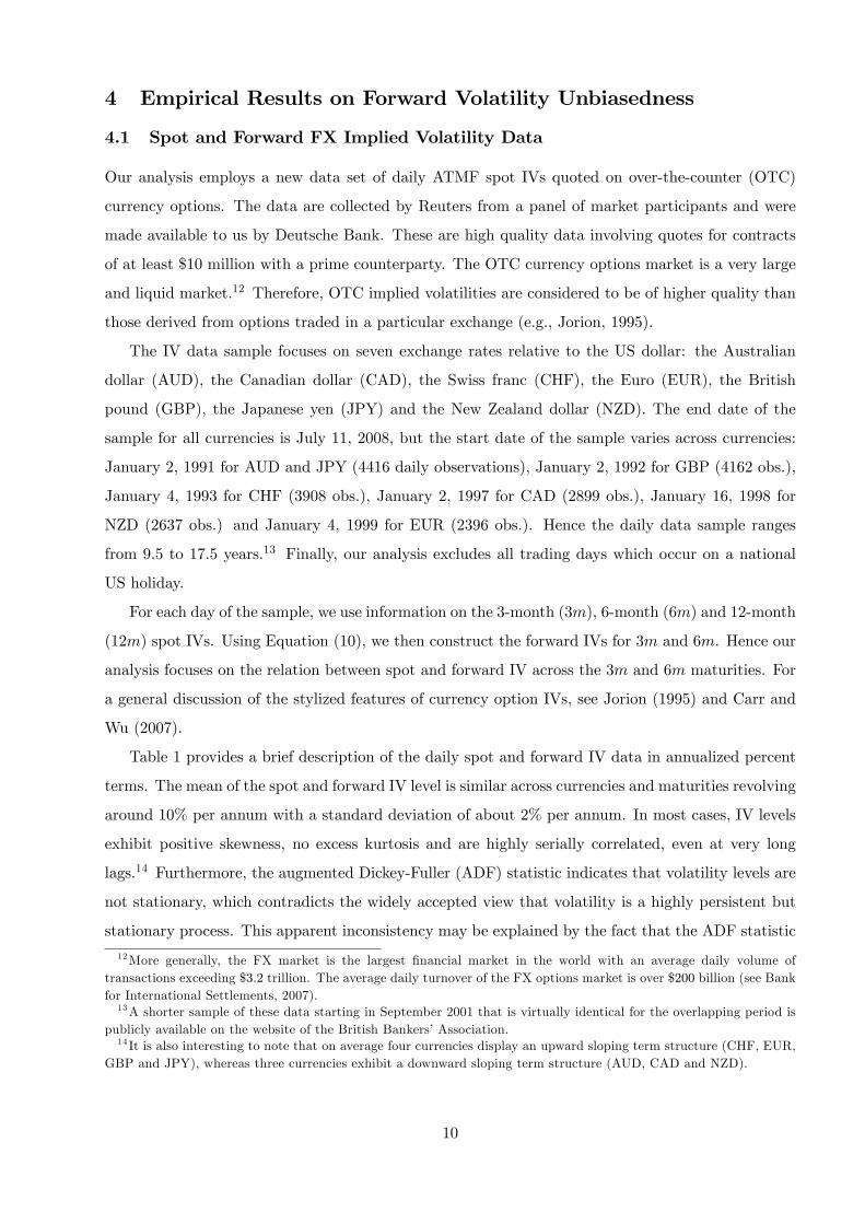
Table 1 provides a brief description of the daily spot and forward IV data in annualized percent

terms. The mean of the spot and forward IV level is similar across currencies and maturities revolving

around 10% per annum with a standard deviation of about 2% per annum. In most cases, IV levels

exhibit positive skewness, no excess kurtosis and are highly serially correlated, even at very long

lags.14 Furthermore, the augmented Dickey-Fuller (ADF) statistic indicates that volatility levels are

not stationary, which contradicts the widely accepted view that volatility is a highly persistent but

stationary process. This apparent inconsistency may be explained by the fact that the ADF statistic

12More generally, the FX market is the largest �nancial market in the world with an average daily volume oftransactions exceeding $3:2 trillion. The average daily turnover of the FX options market is over $200 billion (see Bankfor International Settlements, 2007).13A shorter sample of these data starting in September 2001 that is virtually identical for the overlapping period is

publicly available on the website of the British Bankers�Association.14 It is also interesting to note that on average four currencies display an upward sloping term structure (CHF, EUR,

GBP and JPY), whereas three currencies exhibit a downward sloping term structure (AUD, CAD and NZD).

10

has low power and may not reject non-stationarity when applied to a near-unit root process. In

contrast, as we will see below, the evidence on the stationarity of volatility changes is unambiguous.

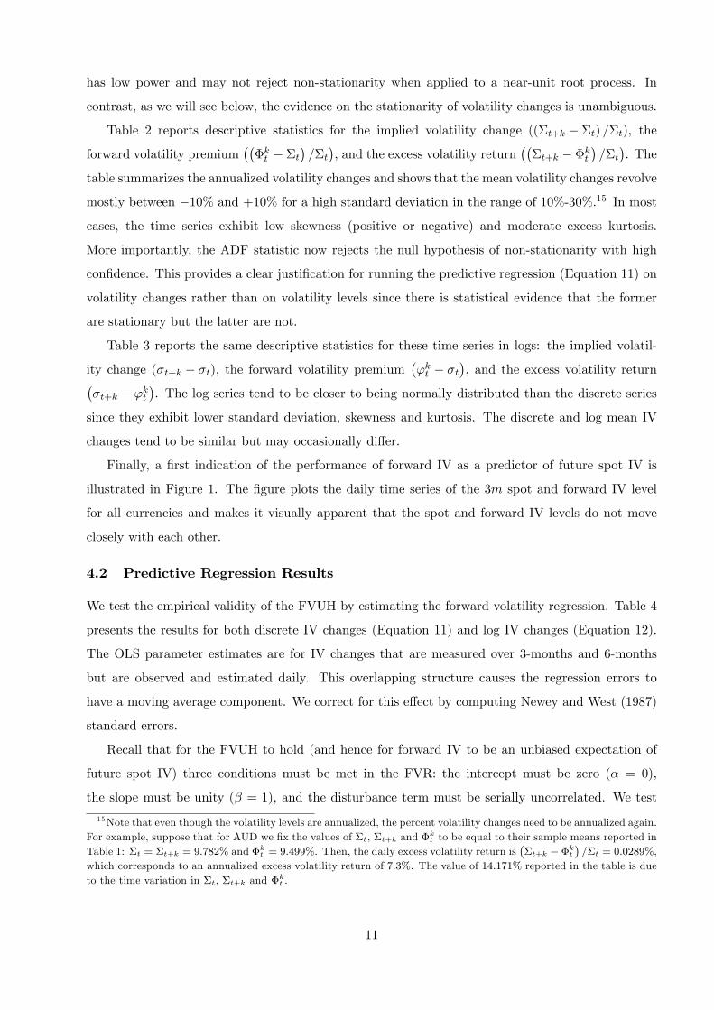
Table 2 reports descriptive statistics for the implied volatility change ((�t+k � �t) =�t), the

forward volatility premium���kt � �t

�=�t

�, and the excess volatility return

���t+k � �kt

�=�t

�. The

table summarizes the annualized volatility changes and shows that the mean volatility changes revolve

mostly between �10% and +10% for a high standard deviation in the range of 10%-30%.15 In most

cases, the time series exhibit low skewness (positive or negative) and moderate excess kurtosis.

More importantly, the ADF statistic now rejects the null hypothesis of non-stationarity with high

con�dence. This provides a clear justi�cation for running the predictive regression (Equation 11) on

volatility changes rather than on volatility levels since there is statistical evidence that the former

are stationary but the latter are not.

Table 3 reports the same descriptive statistics for these time series in logs: the implied volatil-

ity change (�t+k � �t), the forward volatility premium�'kt � �t

�, and the excess volatility return�

�t+k � 'kt�. The log series tend to be closer to being normally distributed than the discrete series

since they exhibit lower standard deviation, skewness and kurtosis. The discrete and log mean IV

changes tend to be similar but may occasionally di¤er.

Finally, a �rst indication of the performance of forward IV as a predictor of future spot IV is

illustrated in Figure 1. The �gure plots the daily time series of the 3m spot and forward IV level

for all currencies and makes it visually apparent that the spot and forward IV levels do not move

closely with each other.

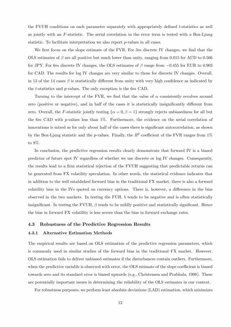
4.2 Predictive Regression Results

We test the empirical validity of the FVUH by estimating the forward volatility regression. Table 4

presents the results for both discrete IV changes (Equation 11) and log IV changes (Equation 12).

The OLS parameter estimates are for IV changes that are measured over 3-months and 6-months

but are observed and estimated daily. This overlapping structure causes the regression errors to

have a moving average component. We correct for this e¤ect by computing Newey and West (1987)

standard errors.

Recall that for the FVUH to hold (and hence for forward IV to be an unbiased expectation of

future spot IV) three conditions must be met in the FVR: the intercept must be zero (� = 0),

the slope must be unity (� = 1), and the disturbance term must be serially uncorrelated. We test

15Note that even though the volatility levels are annualized, the percent volatility changes need to be annualized again.For example, suppose that for AUD we �x the values of �t, �t+k and �kt to be equal to their sample means reported inTable 1: �t = �t+k = 9:782% and �kt = 9:499%. Then, the daily excess volatility return is

��t+k � �kt

�=�t = 0:0289%,

which corresponds to an annualized excess volatility return of 7:3%. The value of 14:171% reported in the table is dueto the time variation in �t, �t+k and �kt .

11

the FVUH conditions on each parameter separately with appropriately de�ned t-statistics as well

as jointly with an F -statistic. The serial correlation in the error term is tested with a Box-Ljung

statistic. To facilitate interpretation we also report p-values in all cases.

We �rst focus on the slope estimate of the FVR. For 3m discrete IV changes, we �nd that the

OLS estimates of � are all positive but much lower than unity, ranging from 0:015 for AUD to 0:566

for JPY. For 6m discrete IV changes, the OLS estimates of � range from �0:455 for EUR to 0:903

for CAD. The results for log IV changes are very similar to those for discrete IV changes. Overall,

in 13 of the 14 cases � is statistically di¤erent from unity with very high con�dence as indicated by

the t-statistics and p-values. The only exception is the 6m CAD.

Turning to the intercept of the FVR, we �nd that the value of � consistently revolves around

zero (positive or negative), and in half of the cases it is statistically insigni�cantly di¤erent from

zero. Overall, the F -statistic jointly testing f� = 0; � = 1g strongly rejects unbiasedness for all but

the 6m CAD with p-values less than 1%. Furthermore, the evidence on the serial correlation of

innovations is mixed as for only about half of the cases there is signi�cant autocorrelation, as shown

by the Box-Ljung statistic and the p-values. Finally, the R2 coe¢ cient of the FVR ranges from 1%

to 8%.

In conclusion, the predictive regression results clearly demonstrate that forward IV is a biased

predictor of future spot IV regardless of whether we use discrete or log IV changes. Consequently,

the results lead to a �rm statistical rejection of the FVUH suggesting that predictable returns can

be generated from FX volatility speculation. In other words, the statistical evidence indicates that

in addition to the well established forward bias in the traditional FX market, there is also a forward

volatility bias in the IVs quoted on currency options. There is, however, a di¤erence in the bias

observed in the two markets. In testing the FUH, b tends to be negative and is often statistically

insigni�cant. In testing the FVUH, � tends to be mildly positive and statistically signi�cant. Hence

the bias in forward FX volatility is less severe than the bias in forward exchange rates.

4.3 Robustness of the Predictive Regression Results

4.3.1 Alternative Estimation Methods

The empirical results are based on OLS estimation of the predictive regression parameters, which

is commonly used in similar studies of the forward bias in the traditional FX market. However,

OLS estimation fails to deliver unbiased estimates if the disturbances contain outliers. Furthermore,

when the predictive variable is observed with error, the OLS estimate of the slope coe¢ cient is biased

towards zero and its standard error is biased upwards (e.g., Christensen and Prabhala, 1998). These

are potentially important issues in determining the reliability of the OLS estimates in our context.

For robustness purposes, we perform least absolute deviations (LAD) estimation, which minimizes

12

the sum of the absolute value of the residuals. The LAD estimator is robust to thick-tailed error

distributions and outliers (e.g., Bassett and Koenker, 1978). Following Carr and Wu (2009), we also

carry out errors-in-variables (EIV) estimation assuming that forward IV is observed with error and

the true value follows an AR(1) process. EIV estimation is based on maximum likelihood and the

Kalman �lter.

The OLS, LAD and EIV estimates for � on both discrete and log IV changes are displayed in

Table 5. The results show that the � estimates are very similar across the three estimation methods.

Hence the FVUH is strongly rejected even when accounting for the e¤ect of outliers or measurement

error. The rest of our analysis uses the OLS parameter estimates.

4.3.2 Subsample Results

Although our data sample on daily IV starts in 1991 spanning 18 years, the FVA contracts came

into existence in the late 1990s. It is therefore interesting to re-examine the predictive regression

results for the shorter subsample of January 4, 1999 to July 11, 2008. This coincides with the period

when trading FVAs and other volatility derivatives surged.16 The subsample results in Table 6 are

qualitatively very similar to the full sample results in Table 4 and generally con�rm the rejection

of the FVUH. The majority of the � estimates tend to be similar across the two samples at values

closer to zero than unity, and remain statistically signi�cant. The single exception is the GBP, which

for the subsample tends to be close to unbiasedness both for 3-month and 6-month maturities. In

contrast to the full sample results, the FVUH is now rejected for the 6-month Canadian dollar. In

general, the subsample analysis con�rms the main full sample �nding that the FVUH is rejected by

the data.

4.3.3 The Cross-Section of Dealers

The IV quotes used in our analysis come from a poll of dealers. Averaging IV quotes across dealers

is a source of measurement error, which is potentially severe in the presence of large outliers. We

directly account for the e¤ect of the distribution of volatilities across dealers on testing the FVUH

by using a separate data set on IV quotes from �ve individual dealers. The data are taken from

Bloomberg and are for three US dollar exchange rates over a shorter sample from January 4, 1999

to July 11, 2008 for the Bank of Tokyo-Mitsubishi UFJ and Tullet Prebon, and from December 15,

2005 to July 11, 2008 for TFS-ICAP, Bank of America and GFI Group. We use this new data set as

there are no dealer data available on the full sample.

Panel A of Table 7 reports descriptive statistics on daily spot and forward IV for the cross-section

16Trading in volatility derivatives took o¤ in the aftermath of the LTCM meltdown in late 1998, when implied stockindex volatility levels rose to unprecedented levels (e.g., Gatheral, 2006).

13

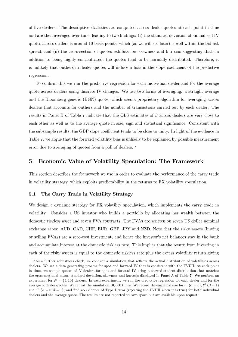
of �ve dealers. The descriptive statistics are computed across dealer quotes at each point in time

and are then averaged over time, leading to two �ndings: (i) the standard deviation of annualized IV

quotes across dealers is around 10 basis points, which (as we will see later) is well within the bid-ask

spread; and (ii) the cross-section of quotes exhibits low skewness and kurtosis suggesting that, in

addition to being highly concentrated, the quotes tend to be normally distributed. Therefore, it

is unlikely that outliers in dealer quotes will induce a bias in the slope coe¢ cient of the predictive

regression.

To con�rm this we run the predictive regression for each individual dealer and for the average

quote across dealers using discrete IV changes. We use two forms of averaging: a straight average

and the Bloomberg generic (BGN) quote, which uses a proprietary algorithm for averaging across

dealers that accounts for outliers and the number of transactions carried out by each dealer. The

results in Panel B of Table 7 indicate that the OLS estimates of � across dealers are very close to

each other as well as to the average quote in size, sign and statistical signi�cance. Consistent with

the subsample results, the GBP slope coe¢ cient tends to be close to unity. In light of the evidence in

Table 7, we argue that the forward volatility bias is unlikely to be explained by possible measurement

error due to averaging of quotes from a poll of dealers.17

5 Economic Value of Volatility Speculation: The Framework

This section describes the framework we use in order to evaluate the performance of the carry trade

in volatility strategy, which exploits predictability in the returns to FX volatility speculation.

5.1 The Carry Trade in Volatility Strategy

We design a dynamic strategy for FX volatility speculation, which implements the carry trade in

volatility. Consider a US investor who builds a portfolio by allocating her wealth between the

domestic riskless asset and seven FVA contracts. The FVAs are written on seven US dollar nominal

exchange rates: AUD, CAD, CHF, EUR, GBP, JPY and NZD. Note that the risky assets (buying

or selling FVAs) are a zero-cost investment, and hence the investor�s net balances stay in the bank

and accumulate interest at the domestic riskless rate. This implies that the return from investing in

each of the risky assets is equal to the domestic riskless rate plus the excess volatility return giving

17As a further robustness check, we conduct a simulation that re�ects the actual distribution of volatilities acrossdealers. We set a data generating process for spot and forward IV that is consistent with the FVUH. At each pointin time, we sample quotes of N dealers for spot and forward IV using a skewed-student distribution that matchesthe cross-sectional mean, standard deviation, skewness and kurtosis displayed in Panel A of Table 7. We perform anexperiment for N = f5; 10g dealers. In each experiment, we run the predictive regression for each dealer and for theaverage of dealer quotes. We repeat the simulation 10; 000 times. We record the empirical size for t� (� = 0), t� (� = 1)and F f� = 0;� = 1g, and �nd no evidence of Type I error (rejecting the FVUH when it is true) for both individualdealers and the average quote. The results are not reported to save space but are available upon request.

14

a total return of it +��t+k � �kt

�=�t for discrete IV changes or it + �t+k � 'kt for log IV changes.

The return from domestic riskless investing is equal to the yield of a US bond proxied by the daily

3-month or 6-month US Eurodeposit rate.

The main objective of our analysis is to determine whether there is economic value in predicting

the returns to volatility speculation due to a possible systematic bias in the way the market sets

forward IV. We consider two strategies for the conditional mean of the returns to volatility speculation

based on the FVUH model and the FVR model. Throughout the analysis we do not model the

dynamics of the conditional covariance matrix of the returns to volatility speculation. In this setting,

the optimal weights will vary across the two models only to the extent that there are deviations from

forward volatility unbiasedness. In particular, the FVR model exploits predictability in the returns

to volatility speculation in the sense that we can use the predictive regression to provide the forecast�Et�t+k � �kt

�=�t (or Et�t+k�'kt ). In contrast, the FVUH benchmark model is equivalent to riskless

investing since �xing � = 0; � = 1 implies that the conditional expectation of excess volatility returns

is equal to zero:�Et�t+k � �kt

�=�t = 0 (or Et�t+k � 'kt = 0).

The investor rebalances her portfolio on a daily basis by taking a position on FX volatility over

a horizon of three or six months ahead. Hence the rebalancing frequency is not the same as the

horizon over which FVA returns are measured. This is sensible for an investor who exploits the daily

arrival of FVA quotes de�ned over alternative maturities. Each day the investor takes two steps.

First, she uses the two models (FVUH and FVR) to forecast the returns to volatility speculation.

Second, conditional on the forecasts, she dynamically rebalances her portfolio by computing the new

optimal weights for the mean-variance strategy described below. This setup is designed to inform us

whether a possible bias in forward volatility a¤ects the performance of an allocation strategy in an

economically meaningful way. We repeat this exercise for the 3-month and 6-month FVA contracts.

We refer to the dynamic strategy implied by the FVR model as the carry trade in volatility

(CTV) strategy. The dynamic CTV strategy can be thought of as the volatility analogue to the

traditional carry trade in currency (CTC) strategy studied, among others, by Burnside et al. (2008)

and Della Corte, Sarno and Tsiakas (2009). The only risk an investor following the CTV strategy is

exposed to is FX volatility risk.

5.2 Mean-Variance Dynamic Asset Allocation

Mean-variance analysis is a natural framework for assessing the economic value of strategies that

exploit predictability in the mean and variance. We design a maximum expected return strategy,

which leads to a portfolio allocation on the e¢ cient frontier. Consider an investor who on a daily

basis constructs a dynamically rebalanced portfolio that maximizes the conditional expected return

subject to achieving a target conditional volatility. Computing the dynamic weights of this portfolio

15

requires k-step ahead forecasts of the conditional mean and the conditional covariance matrix. Let

rt+k denote the N � 1 vector of risky asset returns; �t+kjt = Et [rt+k] is the conditional expectation

of rt+k; and Vt+kjt = Et

��rt+k � �t+kjt

��rt+k � �t+kjt

�0�is the conditional covariance matrix of

rt+k. At each period t, the investor solves the following problem:

maxwt

n�p;t+kjt = w

0t�t+kjt +

�1� w0t�

�rf

os.t.

���p�2= w0tVt+kjtwt; (13)

where wt is the N � 1 vector of portfolio weights on the risky assets, � is an N � 1 vector of ones,

�p;t+kjt is the conditional expected return of the portfolio, ��p is the target conditional volatility of

the portfolio returns, and rf is the return on the riskless asset. The solution to this optimization

problem delivers the risky asset weights:

wt =��ppCtV �1t+kjt

��t+kjt � �rf

�; (14)

where Ct =��t+kjt � �rf

�0V �1t+kjt

��t+kjt � �rf

�. The weight on the riskless asset is 1 � w0t�. Then,

the period t+ k gross return on the investor�s portfolio is:

Rp;t+k = 1 + rp;t+k = 1 +�1� w0t�

�rf + w

0trt+k: (15)

Note that we assume that Vt+kjt = V , where V is the unconditional covariance matrix of IV

changes.

5.3 Performance Measure

We evaluate the performance of the CTV strategy relative to the FVUH benchmark using the

Goetzmann, Ingersoll, Spiegel and Welch (2007) manipulation-proof performance measure de�ned

as:

� =1

(1� �) ln"1

T

T�kXt=1

�R�p;t+kRp;t+k

�1��#; (16)

where R�p;t+k is the gross portfolio return implied by the FVR model, Rp;t+k is implied by the

benchmark FVUH model, and � may be thought of as the investor�s degree of relative risk aversion

(RRA).

As a manipulation-proof performance measure, � is attractive because it is robust to the distrib-

ution of portfolio returns and does not require the assumption of a utility function to rank portfolios.

In contrast, the widely-used certainty equivalent return (e.g., Kandel and Stambaugh, 1996) and the

performance fee (e.g., Fleming, Kirby and Ostdiek, 2001) assume a particular utility function.18 �18The certainty equivalent return is equal to the expected utility of the FVR portfolio returns minus the expected

utility of the FVUH portfolio returns. The Fleming, Kirby and Ostdiek (2001) performance fee is computed by settingthe expected utility of the FVR portfolio returns net of the performance fee to be equal to the expected utility of theFVUH portfolio returns.

16

can be interpreted as the annualized certainty equivalent of the excess portfolio returns and hence

can be viewed as the maximum performance fee an investor will pay to switch from the FVUH to

the FVR strategy. In other words, this criterion measures the risk-adjusted excess return an investor

enjoys for conditioning on the forward volatility bias rather than assuming unbiasedness. We report

� in annualized basis points.

6 Economic Value of Volatility Speculation: The Results

We assess the economic value of the forward volatility bias by analyzing the performance of dy-

namically rebalanced portfolios based on the CTV strategy relative to the FVUH benchmark. The

economic evaluation is conducted both in sample and out of sample. The in-sample period ranges

from January 2, 1991 to July 11, 2008. Since the IV data do not start on the same date for all

currencies, we add risky assets in the portfolio allocation as data on them become available. The last

currency to be added is the euro for which the data sample starts in January 1999. The out-of-sample

period starts at the beginning of the sample (January 1991) and proceeds forward by sequentially

updating the parameter estimates of the FVR day-by-day using a 3-year rolling window.19

Our economic evaluation focuses on the Goetzmann et al. (2007) performance measure, �,

which does not require the assumption of a particular utility function. � is similar to the certainty

equivalent return and provides a measure of the fee a US investor is willing to pay for switching

from the benchmark FVUH strategy to the dynamic CTV strategy. We report the estimates of �

as annualized fees in basis points for a target annualized portfolio volatility ��p = 10% and � = 6.

The choice of ��p and � is reasonable and consistent with numerous empirical studies (e.g., Fleming,

Kirby and Ostdiek, 2001; Marquering and Verbeek, 2004; Della Corte, Sarno and Thornton, 2008).

We have experimented with di¤erent ��p and � values and found that qualitatively they have little

e¤ect on the asset allocation results discussed below.

Table 8 reports the in-sample and out-of-sample portfolio performance for both discrete and log

IV changes. The results show that there is very high economic value associated with the forward

volatility bias. For discrete IV changes, switching from the static FVUH to the CTV portfolio gives

the following staggering performance: (i) in-sample � = 1804 annual basis points (bps) for investing

in 3-month FVAs and � = 944 bps for 6-month contracts, and (ii) out-of-sample � = 1988 bps for

3m and � = 1256 bps for 6m. These results are also re�ected in the Sharpe ratio (SR), which for

the CTV strategy is as follows: (i) in-sample SR = 1:83 for 3m and SR = 1:12 for 6m, and (ii)

out-of-sample SR = 1:74 for 3m and SR = 1:26 for 6m. The results for discrete and log IV changes

are similar.19Note that we use a rolling estimate of the unconditional covariance matrix V as we move through the out-of-sample

period, conditioning only on information available at the time that forecasts are formed.

17

The portfolio weights on the risky assets (FVAs) required to generate this performance are quite

reasonable. Figure 2 illustrates that the average weights for the 3m CTV strategy revolve from

around �0:25 to +0:25 in-sample and from �0:45 to +0:60 out-of-sample. The �gure also displays

the 95% interval of the variation in the weights, which in most cases ranges between �1 and +1. In

short, therefore, the CTV strategy vastly outperforms the FVUH while taking reasonable positions

in the FVAs.

7 Robustness and Further Analysis

7.1 Subsample Results

This section discusses the robustness of the economic value results. To begin with, we evaluate the

performance of the CTV strategy for the shorter subsample period of January 4, 1999 to July 11,

2008. As mentioned before, this coincides with the period when trading FVAs and other volatility

derivatives surged. Panel A of Table 9 displays the in-sample and out-of-sample results for the

subsample, where the out-of-sample period starts on January 4, 1999 and proceeds forward using a

3-year rolling window. Note that for all examples discussed in this section we focus on discrete IV

changes.

The results suggest that the economic value of volatility speculation is slightly higher for the

subsample than for the full sample. For instance, the out-of-sample Sharpe ratio rises from 1:74 for

the 3m full sample to 1:97 for the 3m subsample, and from 1:26 for the 6m full sample to 1:63 for

the 6m subsample. Therefore, the high economic value of the forward volatility bias is not likely to

be due to the choice of a long sample period.

7.2 Portfolio Rebalancing with Non-Overlapping Returns

Our analysis has so far focused on daily rebalancing, where the investor takes positions every day

on 3-month and 6-month ahead IV. An alternative way of evaluating the forward volatility bias

is to consider portfolio rebalancing at the much lower frequencies of quarterly for 3-month ahead

strategies and semi-annual for 6-month ahead strategies. This is equivalent to rebalancing only after

the FVAs have expired. This approach is easier to implement and involves much lower transaction

costs but discards most of the IV information that arrives daily. The 3m strategy now uses 4 return

observations per year as opposed to 252, whereas the 6m strategy only uses 2 observations per year.

Due to the drastic reduction in the number of portfolio return observations we only show in-sample

results for both the full sample and the subsample in Panel B of Table 9. Quite simply, there are not

enough data to run a reliable out-of-sample exercise with quarterly and semi-annual rebalancing.

The results indicate that there is high economic value in the forward volatility bias even when

18

rebalancing infrequently. For quarterly rebalancing, the full sample CTV strategy delivers SR = 1:62

and � = 1658 bps, whereas for semi-annual rebalancing SR = 0:86 and � = 637 bps. The portfolio

performance of the CTV strategy is certainly lower than for daily rebalancing but the CTV still

substantially outperforms the FVUH benchmark. The results for the subsample are slightly better.

Overall, there is robust economic value in the CTV strategy even when rebalancing at low frequency.

7.3 Is Implied Volatility a Random Walk?

Given that the � estimate is much closer to zero (i.e., spot IV is a random walk) than unity (i.e.,

forward volatility unbiasedness), it would be interesting to determine whether in future work the

random walk model for IV would be a sensible benchmark for assessing the economic value of pre-

dictability in the returns to volatility speculation.20 As a further robustness check, Panel C of Table 9

presents the out-of-sample portfolio performance of the random walk with drift (RW) model against

the FVUH benchmark for daily rebalancing. The RW model uses the OLS estimate of the intercept

(�) of the FVR but imposes a slope coe¢ cient of � = 0. The table shows that the out-of-sample

economic value of the RW model is virtually identical to the CTV strategy. For the 3m strategy, the

CTV generates SR = 1:74 and � = 1988 bps, whereas the RW generates SR = 1:83 and � = 1929

bps. For the 6m strategies, the CTV generates SR = 1:26 and � = 1256 bps, whereas the RW

generates SR = 1:18 and � = 1103 bps. These results clearly suggest that the RW model is a useful

benchmark to adopt in future studies of forecasting FX implied volatility.

7.4 Carry Trade in Volatility vs. Carry Trade in Currency

One question that arises naturally from our results is whether the high economic value of the forward

volatility bias (CTV strategy) in the FX options market is related to the economic value of the forward

bias (CTC strategy) in the traditional FX market. In other words, it is interesting to understand

whether the returns to volatility speculation are correlated with the returns to currency speculation.

If the correlation between these two strategies is high, then the forward bias in the FX market and

the FX options market may be potentially driven by the same underlying cause.

We address this issue by designing a dynamic strategy for currency speculation that closely

corresponds to the strategy for volatility speculation described in Section 5.1. Speci�cally, we consider

a US investor who builds a portfolio by allocating her wealth between the domestic riskless asset and

seven forward exchange rates. The seven forward rates are for the same exchange rates and the same

sample range as the volatility speculation strategy investing in the seven FVAs. We then use the

original Fama regression (Equation 4) and the same mean-variance framework to assess the economic

20 Indeed, the majority of studies in the traditional FX market tend to use the random walk of Meese and Rogo¤(1983) as the benchmark model, not forward unbiasedness.

19

value of predictability in exchange rate returns. In essence, we provide an economic evaluation of

the CTC strategy for the same exchange rate sample.

The simplest way of assessing the relation of the CTV strategy with the CTC strategy is to ex-

amine the correlation in their portfolio returns (net of the riskless rate). We compute this correlation

and we �nd that for daily rebalancing it is 0:06 for 3m contracts and 0:14 for 6m. For quarterly

rebalancing (3m) it is 0:11, whereas for semi-annual rebalancing (6m) it is �0:03. Therefore, the

returns to the CTV and CTC strategies seem to be largely uncorrelated.

A more involved way of addressing this issue is to compare the separate portfolio performance of

each of the two strategies with that of a combined strategy. The combined portfolio is constructed by

investing in the same US bond as before and 14 risky assets: the seven FVAs plus the seven forward

exchange rates. Table 8 presents the in-sample and out-of-sample results, which are indicative of the

low correlation between the CTV and the CTC strategies. We focus on the out-of-sample results for

discrete IV changes. In examining the two strategies separately, we observe that the CTV strategy

has superior performance to the CTC strategy. For instance, the 3-month contracts give a Sharpe

ratio of 1:74 for the CTV versus 1:51 for the CTC. The performance measure is 1988 bps and 1522

bps respectively.21

More importantly, however, the combined strategy performs better than the CTV strategy alone.

As we move from the CTV to the combined strategy, the Sharpe ratio rises from 1:74 to 2:48 for 3m

and from 1:26 to 2:03 for 6m. The performance measure increases from 1988 bps to 3290 bps for 3m

and from 1256 bps to 3110 bps for 6m. The clear increase in the economic value when combining CTV

with CTC is evidence that there is distinct incremental information in the CTC over and above the

information already incorporated in the CTV. Therefore, we can conclude that the forward volatility

bias is largely distinct from the forward bias.

Finally, we turn to Figure 3, which illustrates the rolling Sharpe ratios for the 3m and 6m out-of-

sample CTV and CTC strategies using a three-year rolling window. The �gure shows that the SRs

tend to be uncorrelated for long periods of time, especially during the last few years of the sample

when all assets are available for inclusion in the portfolio. Moreover, it is interesting to note that for

the years 2007 and 2008 the SR of the CTV displays a clear upward trend but the SR of the CTC

exhibits a clear downward trend. This indicates that the CTV has done well during the recent credit

crunch when the CTC has not. In other words, this is further evidence that the returns to volatility

speculation tend to be uncorrelated with the returns to currency speculation even during the recent

unwinding of the carry trade in currency.

21 It is worth noting that simple carry trades exploiting the forward bias in the traditional FX market have beenvery pro�table over the years (e.g., Galati and Melvin, 2004; and Brunnermeier, Nagel and Pedersen, 2009). Our�ndings demonstrate that volatility speculation strategies can in fact be even more pro�table than currency speculationstrategies.

20

7.5 Transaction Costs

The impact of transaction costs is an essential consideration in assessing the pro�tability of the

dynamic CTV strategy relative to the riskless FVUH strategy. For instance, if the bid-ask spread in

trading FVAs is su¢ ciently high, the CTV strategy may be too costly to implement. We assess the

e¤ect of transaction costs on the economic value of volatility speculation by directly accounting for

the quoted FVA bid-ask spread. In particular, we use the average quoted FVA bid-ask spread over

the last decade provided by Deutsche Bank. Panel A of Table 10 shows that the spread ranges from

23 to 85 bps, but in most cases revolves around 30 bps.22

It is well-documented that the e¤ective spread is generally lower than the quoted spread, since

trading will take place at the best price quoted at any point in time, suggesting that the worse quotes

will not attract trades (e.g., Mayhew, 2002; De Fontnouvelle, Fishe and Harris, 2003; Battalio, Hatch

and Jennings, 2004). Following Goyal and Saretto (2009), we consider e¤ective transaction costs in

the range of 50% to 100% of the quoted spread. We then follow Marquering and Verbeek (2004)

by deducting the transaction cost from the excess volatility returns ex post. This ignores the fact

that dynamic portfolios are no longer optimal in the presence of transaction costs but maintains

simplicity and tractability in our analysis.

Panel B of Table 10 shows that in the presence of transaction costs the out-of-sample economic

value of volatility speculation with daily rebalancing diminishes but remains positive and high. For

example, when the e¤ective spread is 50% of the quoted spread the 3-month CTV strategy leads to

an out-of-sample SR = 1:27 and � = 1266 bps. The values decrease to SR = 0:75 and � = 502 bps

when the e¤ective spread is equal to the quoted spread. We conclude that accounting for the bid-ask

spread will lower, but not eliminate, the high economic value of volatility speculation.

7.6 Is there a Volatility Term Premium?

We de�ne the percent volatility term premium as the conditional excess volatility return, which is

equal to�Et�t+k � �kt

�=�t for discrete IV changes and Et�t+k � �kt for log IV changes. Under the

FVUH, the percent volatility term premium should be equal to zero. Our empirical results have

so far established that: (i) the unconditional (sample average) volatility term premium is non-zero

and can be either positive or negative (see Tables 2 and 3); (ii) the volatility term premium is

time-varying and predictable when conditioning on the forward volatility premium as shown in the

predictive regression (see Table 4); (iii) there is high economic value in predicting the volatility term

premium of a mean-variance portfolio leading to a highly pro�table carry trade in volatility strategy

(see Table 8); and (iv) the economic performance of the random walk model is very similar to that

22The bid-ask spread will likely vary over time. However, as we only have data on the midquote of IVs we use theaverage bid-ask spread.

21

of the carry trade in volatility strategy (see Table 9).

These results motivate a simple strategy designed to provide a more careful examination of

the volatility term premium for each individual FVA rather than a portfolio of FVAs. Consider an

investor who goes long on an FVA when �t > �kt and short on an FVA when �kt > �t. The conditional

return of this strategy is��t+k � �kt

�=�t � sign

��t � �kt

�, which is simply a reformulation of the

volatility term premium. This strategy is consistent with the random walk model for spot IV.

Table 11 shows that in 13 of the 14 cases the volatility term premium is positive with an annualized

conditional mean ranging between 5%-30% and an annualized standard deviation around 20%-40%.

Not surprisingly, the single exception is the 6m CAD for which we have seen that the FVUH holds

empirically. The percent volatility term premiums tend to have low skewness (positive or negative),

low excess kurtosis and are highly persistent. Using log IV changes reduces the kurtosis of the

percent volatility term premiums and makes them closer to being normally distributed. Finally,

it is important to note that the correlation between on the one hand the percent volatility term

premium (de�ned as�Et�t+k � �kt

�=�t), which is the return to volatility speculation, and on the

other hand the excess currency return (de�ned as�EtSt+k � F kt

�=St), which is the return to currency

speculation, is very low revolving around zero and being positive half of the time. This is further

evidence that what causes a violation of the FVUH is uncorrelated with what causes a violation

of the FUH. Similar results are obtained for log IV changes. In short, we can conclude that the

volatility term premium is conditionally positive, time-varying, predictable and largely uncorrelated

with the return to currency speculation.

8 Conclusion

The introduction of the forward volatility agreement (FVA) has allowed investors to speculate on the

future volatility of exchange rate returns. An FVA contract determines the forward implied volatility

de�ned over an interval starting at a future date. Forward implied volatility is by design meant to

be an unbiased predictor of future spot implied volatility for all relevant maturities. However, if

there is a bias in the way the market sets forward implied volatility, then the returns to volatility

speculation will be predictable and a carry trade in volatility strategy can be pro�table. Still, there

is no study to date in the foreign exchange literature on the empirical issues surrounding FVAs.

These include the empirical properties of FVAs (e.g., their risk-return tradeo¤), the extent to which

forward implied volatility is a biased predictor of future spot implied volatility, and the economic

value of predictability in the returns to volatility speculation.

This paper �lls this gap in the literature by formulating and testing the forward volatility un-

biasedness hypothesis. Our empirical results provide several insights. First, we �nd statistically

22

signi�cant evidence that forward implied volatility is a systematically biased predictor that overes-

timates future spot implied volatility. This is similar to the tendency of the forward premium to

overestimate the future rate of depreciation of high interest currencies, and the tendency of spot

implied volatility to overestimate future realized volatility. Second, the rejection of the forward

volatility unbiasedness indicates the presence of conditionally positive, time-varying and predictable

volatility term premiums in foreign exchange. Third, there is very high in-sample and out-of-sample

economic value in predicting the returns to volatility speculation in the context of dynamic asset

allocation. The economic gains are robust to reasonable transaction costs and largely uncorrelated

with the gains from currency speculation strategies.

To put these �ndings in context, consider that the empirical rejection of uncovered interest parity

leading to the forward bias puzzle has over the years generated an enormous literature in foreign

exchange. At the same time, the carry trade has been a highly pro�table currency speculation

strategy. As this is the �rst study to establish the volatility analogue to the forward bias puzzle and

demonstrate the high economic value of volatility speculation strategies, there are certainly many

directions in which our analysis can be extended. These may involve using alternative data sets,

improvements in the econometric techniques and the empirical setting, re�nements in the framework

for the economic evaluation of realistic trading strategies and, �nally, the development of theoretical

models aiming at explaining these �ndings and rationalizing the volatility term premium. Having

established the main result motivating such extensions, we leave these for future research.

23

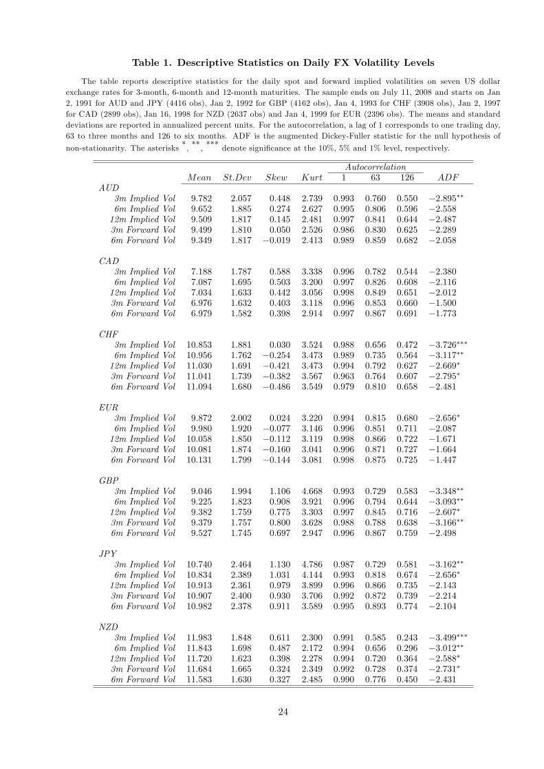
Table 1. Descriptive Statistics on Daily FX Volatility Levels

The table reports descriptive statistics for the daily spot and forward implied volatilities on seven US dollarexchange rates for 3-month, 6-month and 12-month maturities. The sample ends on July 11, 2008 and starts on Jan2, 1991 for AUD and JPY (4416 obs), Jan 2, 1992 for GBP (4162 obs), Jan 4, 1993 for CHF (3908 obs), Jan 2, 1997for CAD (2899 obs), Jan 16, 1998 for NZD (2637 obs) and Jan 4, 1999 for EUR (2396 obs). The means and standarddeviations are reported in annualized percent units. For the autocorrelation, a lag of 1 corresponds to one trading day,63 to three months and 126 to six months. ADF is the augmented Dickey-Fuller statistic for the null hypothesis of

non-stationarity. The asterisks *, **, *** denote signi�cance at the 10%, 5% and 1% level, respectively.

AutocorrelationMean St:Dev Skew Kurt 1 63 126 ADF

AUD3m Implied Vol 9:782 2:057 0:448 2:739 0:993 0:760 0:550 �2:895��6m Implied Vol 9:652 1:885 0:274 2:627 0:995 0:806 0:596 �2:55812m Implied Vol 9:509 1:817 0:145 2:481 0:997 0:841 0:644 �2:4873m Forward Vol 9:499 1:810 0:050 2:526 0:986 0:830 0:625 �2:2896m Forward Vol 9:349 1:817 �0:019 2:413 0:989 0:859 0:682 �2:058

CAD3m Implied Vol 7:188 1:787 0:588 3:338 0:996 0:782 0:544 �2:3806m Implied Vol 7:087 1:695 0:503 3:200 0:997 0:826 0:608 �2:11612m Implied Vol 7:034 1:633 0:442 3:056 0:998 0:849 0:651 �2:0123m Forward Vol 6:976 1:632 0:403 3:118 0:996 0:853 0:660 �1:5006m Forward Vol 6:979 1:582 0:398 2:914 0:997 0:867 0:691 �1:773

CHF3m Implied Vol 10:853 1:881 0:030 3:524 0:988 0:656 0:472 �3:726���6m Implied Vol 10:956 1:762 �0:254 3:473 0:989 0:735 0:564 �3:117��12m Implied Vol 11:030 1:691 �0:421 3:473 0:994 0:792 0:627 �2:669�3m Forward Vol 11:041 1:739 �0:382 3:567 0:963 0:764 0:607 �2:795�6m Forward Vol 11:094 1:680 �0:486 3:549 0:979 0:810 0:658 �2:481

EUR3m Implied Vol 9:872 2:002 0:024 3:220 0:994 0:815 0:680 �2:656�6m Implied Vol 9:980 1:920 �0:077 3:146 0:996 0:851 0:711 �2:08712m Implied Vol 10:058 1:850 �0:112 3:119 0:998 0:866 0:722 �1:6713m Forward Vol 10:081 1:874 �0:160 3:041 0:996 0:871 0:727 �1:6646m Forward Vol 10:131 1:799 �0:144 3:081 0:998 0:875 0:725 �1:447

GBP3m Implied Vol 9:046 1:994 1:106 4:668 0:993 0:729 0:583 �3:348��6m Implied Vol 9:225 1:823 0:908 3:921 0:996 0:794 0:644 �3:093��12m Implied Vol 9:382 1:759 0:775 3:303 0:997 0:845 0:716 �2:607�3m Forward Vol 9:379 1:757 0:800 3:628 0:988 0:788 0:638 �3:166��6m Forward Vol 9:527 1:745 0:697 2:947 0:996 0:867 0:759 �2:498

JPY3m Implied Vol 10:740 2:464 1:130 4:786 0:987 0:729 0:581 �3:162��6m Implied Vol 10:834 2:389 1:031 4:144 0:993 0:818 0:674 �2:656�12m Implied Vol 10:913 2:361 0:979 3:899 0:996 0:866 0:735 �2:1433m Forward Vol 10:907 2:400 0:930 3:706 0:992 0:872 0:739 �2:2146m Forward Vol 10:982 2:378 0:911 3:589 0:995 0:893 0:774 �2:104

NZD3m Implied Vol 11:983 1:848 0:611 2:300 0:991 0:585 0:243 �3:499���6m Implied Vol 11:843 1:698 0:487 2:172 0:994 0:656 0:296 �3:012��12m Implied Vol 11:720 1:623 0:398 2:278 0:994 0:720 0:364 �2:588�3m Forward Vol 11:684 1:665 0:324 2:349 0:992 0:728 0:374 �2:731�6m Forward Vol 11:583 1:630 0:327 2:485 0:990 0:776 0:450 �2:431

24

Table 2. Descriptive Statistics on Daily Discrete FX Volatility Changes

The table displays descriptive statistics for the daily discrete FX volatility changes on seven US dollar exchange

rates for 3-month and 6-month maturities. The Implied Volatility Change is de�ned as (�t+k � �t) =�t, where �tis the annualized spot implied volatility over the period t to t+k, and �t+k is for t+k to t+2k. The Forward VolatilityPremium is de�ned as

��kt � �t

�=�t, where �

kt is the annualized forward implied volatility determined at time t

for the period t+k to t+2k. The Excess Volatility Return is de�ned as��t+k � �kt

�=�t. The means and standard

deviations are reported in annualized percent units. For the autocorrelation, a lag of 1 corresponds to one trading day,

63 to three months and 126 to six months. ADF is the augmented Dickey-Fuller statistic for the null hypothesis of

non-stationarity. The asterisks *, **, *** denote signi�cance at the 10%, 5% and 1% level, respectively.

AutocorrelationMean St:Dev Skew Kurt 1 63 126 ADF

AUD3m Implied Vol Change 5:065 30:440 1:063 5:309 0:974 �0:042 �0:032 �6:558���3m Forward Vol Premium �9:107 18:267 0:031 5:568 0:907 0:468 0:312 �4:542���3m Excess Vol Return 14:171 35:357 0:900 4:226 0:972 0:379 0:186 �4:886���6m Implied Vol Change 4:771 27:035 1:206 5:233 0:987 0:527 0:049 �4:215���6m Forward Vol Premium �6:025 10:041 �1:516 8:364 0:868 0:584 0:440 �3:294��6m Excess Vol Return 10:796 29:849 1:007 3:923 0:985 0:653 0:242 �3:813���

CAD3m Implied Vol Change 12:650 37:022 2:762 16:545 0:982 �0:061 �0:186 �4:984���3m Forward Vol Premium �10:038 12:805 �1:872 10:055 0:919 0:128 0:063 �4:839���3m Excess Vol Return 22:688 37:224 2:736 15:952 0:983 0:161 �0:057 �4:717���6m Implied Vol Change 12:175 32:687 2:164 8:915 0:993 0:421 �0:191 �3:516���6m Forward Vol Premium �2:249 5:314 �2:322 14:592 0:923 0:317 0:068 �5:151���6m Excess Vol Return 14:424 32:336 2:237 9:012 0:992 0:469 �0:124 �3:306��

CHF3m Implied Vol Change 3:129 30:408 1:310 5:374 0:968 �0:166 �0:048 �6:686���3m Forward Vol Premium 9:563 15:027 �0:301 7:274 0:756 0:176 �0:006 �5:558���3m Excess Vol Return �6:434 31:352 0:897 4:542 0:950 0:131 0:021 �5:899���6m Implied Vol Change 1:135 23:454 1:141 5:517 0:980 0:445 �0:084 �4:462���6m Forward Vol Premium 3:857 7:733 �0:317 11:250 0:728 0:113 0:029 �5:388���6m Excess Vol Return �2:722 24:049 1:119 6:094 0:975 0:539 0:061 �3:637���

EUR3m Implied Vol Change 4:313 26:666 0:741 3:619 0:971 �0:020 0:059 �5:029���3m Forward Vol Premium 10:470 11:603 0:196 2:945 0:934 0:342 0:192 �4:202���3m Excess Vol Return �6:157 28:580 0:533 3:403 0:978 0:313 0:189 �4:005���6m Implied Vol Change 3:672 24:491 1:051 4:734 0:989 0:615 0:165 �3:016��6m Forward Vol Premium 4:131 5:702 0:334 4:267 0:942 0:450 0:314 �3:944���6m Excess Vol Return �0:458 25:727 0:791 4:050 0:992 0:691 0:276 �2:590�

GBP3m Implied Vol Change 2:884 34:934 1:463 6:993 0:978 �0:186 �0:170 �6:821���3m Forward Vol Premium 18:969 18:954 �0:331 9:726 0:937 0:338 0:264 �6:477���3m Excess Vol Return �16:085 34:753 0:543 4:561 0:979 0:178 �0:046 �5:650���6m Implied Vol Change 1:214 25:239 0:890 4:532 0:989 0:314 �0:278 �5:219���6m Forward Vol Premium 7:619 9:488 0:959 5:333 0:961 0:446 0:261 �5:563���6m Excess Vol Return �6:405 24:754 0:168 4:283 0:990 0:442 �0:072 �4:247���

JPY3m Implied Vol Change 4:943 33:641 0:893 4:304 0:964 �0:229 0:055 �7:788���3m Forward Vol Premium 8:653 16:884 �0:080 3:741 0:920 0:309 0:230 �6:930���3m Excess Vol Return �3:711 33:075 0:626 4:230 0:966 0:169 0:139 �6:340���6m Implied Vol Change 2:905 24:176 0:626 3:847 0:979 0:450 �0:089 �5:732���6m Forward Vol Premium 3:834 8:121 0:014 4:198 0:905 0:279 0:105 �6:318���6m Excess Vol Return �0:929 23:989 0:538 3:816 0:982 0:557 0:069 �4:769���

NZD3m Implied Vol Change 5:816 28:733 0:932 4:681 0:976 �0:075 �0:049 �5:614���3m Forward Vol Premium �9:216 14:715 �0:442 2:792 0:958 0:548 0:414 �4:129���3m Excess Vol Return 15:032 31:262 0:864 3:658 0:984 0:301 0:081 �3:825���6m Implied Vol Change 5:922 24:879 0:808 3:475 0:990 0:478 �0:121 �3:861���6m Forward Vol Premium �4:440 8:452 �0:883 3:891 0:953 0:611 0:489 �3:213��6m Excess Vol Return 10:362 26:074 0:941 3:204 0:989 0:591 0:076 �3:949���

25

Table 3. Descriptive Statistics on Daily Log FX Volatility Changes

The table displays descriptive statistics for the daily log FX volatility changes on seven US dollar exchange rates

for 3-month and 6-month maturities. The Implied Volatility Change is de�ned as �t+k��t, where �t is the log ofthe annualized spot implied volatility over the period t to t+k, and �t+k is for t+k to t+2k. The Forward VolatilityPremium is de�ned as 'kt � �t, where 'kt is the log of the annualized forward implied volatility determined at time tfor the period t+k to t+2k. The Excess Volatility Return is de�ned as �t+k�'kt . The means and standard deviationsare reported in annualized percent units. For the autocorrelation, a lag of 1 corresponds to one trading day, 63 to three

months and 126 to six months. ADF is the augmented Dickey-Fuller statistic for the null hypothesis of non-stationarity.

The asterisks *, **, *** denote signi�cance at the 10%, 5% and 1% level, respectively.

AutocorrelationMean St:Dev Skew Kurt 1 63 126 ADF

AUD3m Implied Vol Change 0:792 28:769 0:498 3:608 0:975 �0:053 �0:040 �6:421���3m Forward Vol Premium �10:993 19:015 �0:491 4:574 0:909 0:472 0:317 �4:602���3m Excess Vol Return 11:786 34:179 0:626 3:261 0:972 0:410 0:197 �4:693���6m Implied Vol Change 1:521 24:847 0:572 3:591 0:987 0:525 0:036 �4:165���6m Forward Vol Premium �6:711 11:231 �2:468 18:401 0:840 0:544 0:402 �3:458���6m Excess Vol Return 8:232 28:225 0:602 2:941 0:980 0:664 0:266 �3:473���

CAD3m Implied Vol Change 7:194 31:129 1:457 7:653 0:981 �0:085 �0:202 �4:821���3m Forward Vol Premium �11:125 14:259 �2:612 16:209 0:915 0:104 0:054 �5:230���3m Excess Vol Return 18:319 31:591 1:515 7:262 0:980 0:200 �0:047 �4:418���6m Implied Vol Change 7:942 26:659 1:324 5:675 0:992 0:412 �0:214 �3:625���6m Forward Vol Premium �2:417 5:666 �2:840 18:037 0:932 0:300 0:061 �5:091���6m Excess Vol Return 10:359 26:115 1:486 5:718 0:992 0:477 �0:133 �3:279��

CHF3m Implied Vol Change �1:045 28:299 0:809 3:860 0:966 �0:179 �0:051 �6:667���3m Forward Vol Premium 8:334 15:128 �1:078 9:923 0:749 0:178 �0:004 �7:681���3m Excess Vol Return �9:378 29:729 0:619 3:811 0:944 0:148 0:022 �5:705���6m Implied Vol Change �1:398 22:192 0:500 3:736 0:980 0:422 �0:104 �4:249���6m Forward Vol Premium 3:524 7:775 �1:244 15:229 0:716 0:106 0:033 �5:265���6m Excess Vol Return �4:922 22:908 0:523 4:304 0:973 0:518 0:049 �3:604���

EUR3m Implied Vol Change 0:943 25:676 0:364 3:041 0:973 �0:037 0:065 �5:700���3m Forward Vol Premium 9:698 11:288 0:035 2:910 0:934 0:352 0:200 �4:215���3m Excess Vol Return �8:755 27:738 0:268 3:087 0:980 0:315 0:202 �4:118���6m Implied Vol Change 0:936 22:963 0:447 3:617 0:990 0:591 0:148 �2:953��6m Forward Vol Premium 3:933 5:564 0:165 3:729 0:945 0:455 0:319 �3:914���6m Excess Vol Return �2:997 24:368 0:277 3:238 0:993 0:675 0:270 �3:461���

GBP3m Implied Vol Change �2:5472 32:244 0:756 4:095 0:977 �0:196 �0:177 �6:932���3m Forward Vol Premium 16:751 19:559 �2:714 34:349 0:920 0:276 0:207 �5:615���3m Excess Vol Return �19:298 33:397 0:402 5:094 0:973 0:200 �0:030 �7:584���6m Implied Vol Change �1:785 24:294 0:243 3:495 0:990 0:320 �0:287 �5:127���6m Forward Vol Premium 7:073 8:938 0:611 5:292 0:960 0:425 0:242 �5:714���6m Excess Vol Return �8:858 24:206 �0:410 4:040 0:991 0:459 �0:067 �4:082���

JPY3m Implied Vol Change �0:324 32:059 0:350 3:282 0:964 �0:235 0:045 �7:584���3m Forward Vol Premium 7:171 16:776 �0:453 4:436 0:915 0:300 0:227 �7:008���3m Excess Vol Return �7:495 31:692 0:190 3:451 0:967 0:185 0:124 �5:452���6m Implied Vol Change 0:111 23:510 0:055 3:253 0:981 0:448 �0:102 �5:764���6m Forward Vol Premium 3:478 8:013 �0:273 4:621 0:897 0:267 0:100 �6:403���6m Excess Vol Return �3:367 23:426 0:013 3:235 0:984 0:553 0:056 �4:818���

NZD3m Implied Vol Change 1:967 27:331 0:416 3:584 0:978 �0:079 �0:055 �5:452���3m Forward Vol Premium �10:492 15:417 �0:631 3:068 0:957 0:549 0:416 �4:225���3m Excess Vol Return 12:459 30:170 0:577 2:944 0:984 0:321 0:083 �3:492���6m Implied Vol Change 3:060 23:345 0:344 3:097 0:991 0:476 �0:126 �3:794���6m Forward Vol Premium �4:880 8:937 �1:121 5:154 0:943 0:603 0:477 �3:252��6m Excess Vol Return 7:940 24:433 0:670 2:738 0:988 0:592 0:086 �3:542���

26

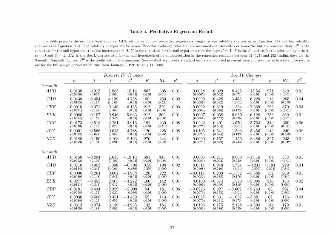
Table 4. Predictive Regression Results

The table presents the ordinary least squares (OLS) estimates for two predictive regressions using discrete volatility changes as in Equation (11) and log volatilitychanges as in Equation (12). The volatility changes are for seven US dollar exchange rates and are measured over 3-months or 6-months but are observed daily. tα is thet-statistic for the null hypothesis that the intercept α = 0. tβ is the t-statistic for the null hypothesis that the slope β = 1. F is the F -statistic for the joint null hypothesisα = 0 and β = 1. BL is the Box-Ljung statistic for the null hypothesis of no autocorrelation in the regression residuals between 64 (127) and 252 trading days for the3-month (6-month) figures. R2 is the coefficient of determination. Newey-West asymptotic standard errors are reported in parentheses and p-values in brackets. The resultsare for the full sample period which runs from January 2, 1991 to July 11, 2008.

Discrete IV Changes Log IV Changesα β tα tβ F BL R2 α β tα tβ F BL R2

3-monthAUD 0.0130

(0.0069)0.015(0.065)

1.885[0.060]

−15.14[<0.01]

807[<0.01]

305[0.013]

0.01 0.0028(0.0065)

0.029(0.062)

0.425[0.671]

−15.54[<0.01]

971[<0.01]

329[<0.01]

0.01

CAD 0.0430(0.0105)

0.454(0.115)

4.109[<0.01]

−4.758[<0.01]

60[<0.01]

250[0.524]

0.02 0.0299(0.0087)

0.428(0.092)

3.453[<0.01]

−6.220[<0.01]

116[<0.01]

265[0.279]

0.04

CHF −0.0010(0.0071)

0.371(0.103)

−0.146[0.884]

−6.135[<0.01]

212[<0.01]

326[<0.01]

0.03 −0.0092(0.0068)

0.319(0.090)

−1.364[0.173]

−7.569[<0.01]

282[<0.01]

370[<0.01]

0.03

EUR 0.0080(0.0084)

0.107(0.158)

0.946[0.345]

−5.633[<0.01]

212[<0.01]

362[<0.01]

0.01 0.0007(0.0081)

0.068(0.152)

0.089[0.929]

−6.128[<0.01]

232[<0.01]

369[<0.01]

0.01

GBP −0.0173(0.0076)

0.518(0.123)

−2.281[0.023]

−3.916[<0.01]

191[<0.01]

239[0.713]

0.08 −0.0232(0.0075)

0.401(0.104)

−3.070[<0.01]

−5.763[<0.01]

340[<0.01]

300[0.021]

0.06

JPY 0.0001(0.0072)

0.566(0.091)

0.015[0.988]

−4.788[<0.01]

120[<0.01]

225[0.887]

0.08 −0.0105(0.0070)

0.541(0.084)

−1.503[0.133]

−5.456[<0.01]

142[<0.01]

240[0.699]

0.08

NZD 0.0180(0.0083)

0.150(0.104)

2.163[0.031]

−8.193[<0.01]

270[<0.01]

244[0.637]

0.01 0.0090(0.0078)

0.157(0.099)

1.156[0.248]

−8.486[<0.01]

327[<0.01]

243[0.642]

0.01

6-monthAUD 0.0150

(0.0092)−0.294(0.106)

1.633[0.103]

−12.18[<0.01]

591[<0.01]

345[<0.01]

0.01 0.0005(0.0085)

−0.211(0.092)

0.063[0.950]

−13.16[<0.01]

764[<0.01]

338[<0.01]

0.01

CAD 0.0710(0.0134)

0.903(0.242)

5.308[<0.01]

−0.400[0.689]

0.58[0.555]

198[1.000]

0.02 0.0511(0.0108)

0.948(0.216)

4.754[<0.01]

−0.241[0.809]

0.194[0.824]

229[0.846]

0.04

CHF 0.0006(0.0089)

0.264(0.148)

0.067[0.947]

−4.988[<0.01]

126[<0.01]

222[1.000]

0.01 −0.0111(0.0082)

0.233(0.135)

−1.352[0.176]

−5.686[<0.01]

152[<0.01]

249[0.540]

0.01

EUR 0.0277(0.0111)

−0.455(0.341)

2.505[0.012]

−4.272[<0.01]

166[<0.01]

142[1.000]

0.01 0.0160(0.0101)

−0.574(0.309)

1.573[0.116]

−5.095[<0.01]

210[<0.01]

153[1.000]

0.02

GBP −0.0181(0.0078)

0.634(0.174)

−2.329[0.020]

−2.099[0.036]

54[<0.01]

181[1.000]

0.06 −0.0275(0.0076)

0.527(0.173)

−3.602[<0.01]

−2.743[<0.01]

83[<0.01]

207[0.980]

0.04

JPY 0.0036(0.0080)

0.568(0.125)

0.451[0.652]

−3.439[<0.01]

52[<0.01]

143[1.000]

0.04 −0.0087(0.0079)

0.531(0.121)

−1.097[0.273]

−3.881[<0.01]

62[<0.01]

163[1.000]

0.03

NZD 0.0313(0.0100)

0.074(0.188)

3.130[0.002]

−4.935[<0.01]

142[<0.01]

164[1.000]

0.01 0.0196(0.0092)

0.175(0.180)

2.128[0.030]

−4.594[<0.01]

144[<0.01]

179[1.000]

0.01

27

Table 5. Predictive Regression Results under Alternative Estimation Methods

The table presents the estimates for two predictive regressions using three estimation methods: ordinary least squares (OLS), least absolute deviation (LAD) anderrors-in-variables (EIV). The first regression uses discrete volatility changes as in Equation (11) and the second regression uses log volatility changes as in Equation (12).The volatility changes are for seven US dollar exchange rates and are measured over 3-months or 6-months but are observed daily. The LAD estimator minimizes the sum ofthe absolute value of residuals and is robust to outliers (Bassett and Koenker, 1978). The EIV method uses maximum likelihood jointly with the Kalman filter to estimatethe parameters when the explanatory variable is measured with error (Carr and Wu, 2009). tβ is the t-statistic for the null hypothesis that the slope β = 1. Asymptoticstandard errors are reported in parentheses and p-values in brackets. OLS uses Newey-West standard errors. LAD uses Weiss (1990) standard errors. The results are forthe full sample period which runs from January 2, 1991 to July 11, 2008.

Discrete IV Changes Log IV ChangesβOLS tβOLS βLAD tβLAD βEIV tβEIV βOLS tβOLS βLAD tβLAD βEIV tβEIV

3-monthAUD 0.015

(0.065)−15.14[<0.01]

0.077(0.069)

−13.30[<0.01]

−0.010(0.028)

−35.96[<0.01]

0.029(0.062)

−15.54[<0.01]

0.057(0.065)

−14.36[<0.01]

0.005(0.069)

−41.27[<0.01]

CAD 0.454(0.115)

−4.758[<0.01]

0.476(0.121)

−4.346[<0.01]

0.471(0.066)

−8.039[<0.01]

0.428(0.092)

−6.220[<0.01]

0.442(0.096)

−5.935[<0.01]

0.445(0.047)

−11.87[<0.01]

CHF 0.371(0.103)

−6.135[<0.01]

0.252(0.110)

−6.807[<0.01]

0.500(0.027)

−18.57[<0.01]

0.319(0.090)

−7.569[<0.01]

0.239(0.095)

−8.020[<0.01]

0.424(0.026)

−22.05[<0.01]

EUR 0.107(0.158)

−5.633[<0.01]

0.049(0.171)

−5.576[<0.01]

0.082(0.041)

−22.59[<0.01]

0.068(0.152)

−6.128[<0.01]

0.032(0.161)

−6.012[<0.01]

0.038(0.041)

−23.27[<0.01]

GBP 0.518(0.123)

−3.916[<0.01]

0.380(0.129)

−4.794[<0.01]

0.531(0.021)

−22.28[<0.01]

0.401(0.104)

−5.763[<0.01]

0.368(0.107)

−5.930[<0.01]

0.410(0.020)

−29.85[<0.01]

JPY 0.566(0.091)

−4.788[<0.01]

0.593(0.096)

−4.258[<0.01]

0.592(0.027)

−14.91[<0.01]

0.541(0.084)

−5.456[<0.01]

0.598(0.088)

−4.562[<0.01]

0.566(0.027)

−16.22[<0.01]

NZD 0.150(0.104)

−8.193[<0.01]

0.076(0.110)

−8.410[<0.01]

0.143(0.040)

−21.22[<0.01]

0.157(0.099)

−8.486[<0.01]

0.059(0.104)

−9.029[<0.01]

0.152(0.035)

−24.05[<0.01]

6-monthAUD −0.294

(0.106)−12.18[<0.01]

−0.305(0.110)

−11.91[<0.01]

−0.462(0.050)

−29.38[<0.01]

−0.211(0.092)

−13.16[<0.01]

−0.271(0.097)

−13.06[<0.01]

−0.378(0.039)

−34.92[<0.01]

CAD 0.903(0.242)

−0.400[0.689]

1.008(0.216)

0.038[0.970]

0.975(0.164)

−0.151[0.880]

0.948(0.216)

−0.241[0.809]

1.033(0.192)

0.170[0.865]

1.013(0.104)

0.128[0.900]

CHF 0.264(0.148)

−4.988[<0.01]

0.303(0.158)

−4.423[<0.01]

0.295(0.045)

−15.80[<0.01]

0.233(0.135)

−5.686[<0.01]

0.283(0.142)

−5.041[<0.01]

0.258(0.043)

−17.32[<0.01]

EUR −0.455(0.341)

−4.272[<0.01]

−1.026(0.386)

−5.253[<0.01]

−0.531(0.073)

−20.87[<0.01]

−0.574(0.309)

−5.095[<0.01]

−1.055(0.400)

−6.050[<0.01]

−0.656(0.074)

−22.35[<0.01]

GBP 0.634(0.174)

−2.099[0.036]

0.565(0.183)

−2.380[0.017]

0.648(0.033)

−10.59[<0.01]

0.527(0.173)

−2.743[<0.01]

0.585(0.181)

−2.292[0.022]

0.535(0.036)

−13.08[0.010]

JPY 0.568(0.125)

−3.439[<0.01]

0.447(0.135)

−4.090[<0.01]

0.597(0.046)

−8.775[<0.01]

0.531(0.121)

−3.881[<0.01]

0.435(0.127)

−4.444[<0.01]

0.560(0.046)

−9.515[<0.01]

NZD 0.074(0.188)

−4.935[<0.01]

−0.104(0.197)

−5.606[<0.01]

0.064(0.059)

−15.82[<0.01]

0.175(0.180)

−4.594[<0.01]

−0.103(0.195)

−5.653[<0.01]

0.175(0.051)

−16.25[<0.01]

28

Table 6. Predictive Regression Results for a Subsample (1999-2008)

The table presents the ordinary least squares (OLS) estimates for two predictive regressions for the sub-sample period of January 4, 1999 to July 11, 2008. The firstregression uses discrete volatility changes as in Equation (11) and the second regression uses log volatility changes as in Equation (12). The volatility changes are for sevenUS dollar exchange rates and are measured over 3-months or 6-months but are observed daily. tα is the t-statistic for the null hypothesis that the intercept α = 0. tβ isthe t -statistic for the null hypothesis that the slope β = 1. F is the F -statistic for the joint null hypothesis α = 0 and β = 1. BL is the Box-Ljung statistic for the nullhypothesis of no autocorrelation in the regression residuals between 64 (127) and 252 trading days for the 3-month (6-month) figures. R2 is the coefficient of determination.Newey-West asymptotic standard errors are reported in parentheses and p-values in brackets.

Discrete IV Changes Log IV Changesα β tα tβ F BL R2 α β tα tβ F BL R2

3-monthAUD 0.0117

(0.0090)0.111(0.097)

1.300[0.194]

−9.133[<0.01]

228[<0.01]

283[0.085]

0.01 0.0019(0.0085)

0.098(0.093)

0.220[0.826]

−9.719[<0.01]

281[<0.01]

299[0.022]

0.01

CAD 0.0185(0.0081)

0.211(0.162)

2.287[0.022]

−4.884[<0.01]

109[<0.01]

280[0.112]

0.01 0.0106(0.0076)

0.218(0.150)

1.388[0.165]

−5.223[<0.01]

130[<0.01]

286[0.068]

0.01

CHF 0.0090(0.0087)

0.138(0.137)

1.035[0.301]

−6.299[<0.01]

221[<0.01]

368[<0.01]

0.01 0.0011(0.0082)

0.119(0.127)

0.139[0.889]

−6.916[<0.01]

246[<0.01]

364[<0.01]

0.01

EUR 0.0080(0.0084)

0.107(0.158)

0.946[0.345]

−5.633[<0.01]

212[<0.01]

362[<0.01]

0.01 0.0007(0.0081)

0.068(0.152)

0.089[0.929]

−6.128[<0.01]

232[<0.01]

369[<0.01]

0.01

GBP −0.0162(0.0080)

0.814(0.174)

−2.023[0.043]

−1.073[0.283]

10.6[<0.01]

261[0.336]

0.11 −0.0218(0.0077)

0.752(0.165)

−2.817[0.005]

−1.498[0.134]

18.3[<0.01]

277[0.137]

0.10

JPY −0.0045(0.0096)

0.425(0.118)

−0.464[0.643]

−4.891[<0.01]

94.0[<0.01]

218[0.942]

0.04 −0.0155(0.0092)

0.405(0.111)

−1.691[0.091]

−5.342[<0.01]

112[<0.01]

252[0.484]

0.04

NZD 0.0155(0.0083)

0.217(0.093)

1.873[0.061]

−8.415[<0.01]

170[<0.01]

285[0.075]

0.01 0.0074(0.0078)

0.197(0.085)

0.943[0.346]

−9.384[<0.01]

216[<0.01]

279[0.118]

0.01

6-monthAUD 0.0247

(0.0119)−0.217(0.168)

2.080[0.038]

−7.258[<0.01]

108[<0.01]

137[1.000]

0.01 0.0092(0.0106)

−0.211(0.158)

0.866[0.387]

−7.683[<0.01]

139[<0.01]

162[1.000]

0.01

CAD 0.0394(0.0114)

0.270(0.318)

3.452[0.001]

−2.296[0.022]

16.94[<0.01]

170[1.000]

0.01 0.0260(0.0099)

0.304(0.291)

2.623[0.009]

−2.394[0.017]

21.3[<0.01]

195[0.997]

0.01

CHF 0.0295(0.0113)

−0.592(0.234)

2.602[0.009]

−6.794[<0.01]

253[<0.01]

140[1.000]

0.03 0.0157(0.0100)

−0.577(0.205)

1.582[0.114]

−7.695[<0.01]

287[<0.01]

151[1.000]

0.03

EUR 0.0277(0.0111)

−0.455(0.340)

2.505[0.012]

−4.272[<0.01]

166[<0.01]

142[1.000]

0.01 0.0160(0.0102)

−0.574(0.309)

1.573[0.116]

−5.095[<0.01]

210[<0.01]

154[1.000]

0.02

GBP −0.0012(0.0097)

0.923(0.347)

−0.129[0.897]

−0.223[0.824]

0.483[0.617]

138[1.000]

0.04 −0.0092(0.0096)

0.784(0.303)

−0.960[0.337]

−0.712[0.476]

4.01[0.0182]

164[1.000]

0.03

JPY −0.0074(0.0102)

0.077(0.158)

−0.720[0.472]

−5.855[<0.01]

105[<0.01]

116[1.000]

0.01 −0.0190(0.0097)

0.086(0.154)

−1.954[0.051]

−5.923[<0.01]

107[<0.01]

126[1.000]

0.01

NZD 0.0286(0.0099)

−0.238(0.145)

2.886[0.004]

−8.543[<0.01]

194[<0.01]

166[1.000]

0.01 0.0171(0.0091)

−0.217(0.127)

1.876[0.061]

−9.596[<0.01]

244[<0.01]

177[1.000]

0.01

29

Table 7. Predictive Regression Results for a Pool of Dealers

Panel A reports descriptive statistics on daily spot and forward implied volatility for a pool of five individual dealers over a sample of three US dollar exchange rates.The sample period runs from January 4, 1999 to July 11, 2008 for the Bank of Tokyo-Mitsubishi UFJ and Tullet Prebon, and from December 15, 2005 to July 11, 2008 forTFS-ICAP, Bank of America and GFI Group. The Bloomberg quote, also known as the Bloomberg generic (BGN) quote, uses a proprietary algorithm for averaging acrossdealers that accounts for outliers and the number of transactions carried out by each dealer. The descriptive statistics are computed across dealer quotes at each point intime and are then averaged over time. Panel B reports the OLS estimates for the predictive regression run for each individual dealer and for the average quote across dealers.The regression uses discrete implied volatility changes, which are measured over 3-months or 6-months but are observed daily. tβ is the t-statistic for the null hypothesisthat the slope β = 1. Newey-West asymptotic standard errors are reported in parentheses and p-values in brackets.

Panel A: Descriptive Statistics for the Cross Section of DealersEUR GBP JPY

Mean St.Dev Skew Kurt Mean St.Dev Skew Kurt Mean St.Dev Skew Kurt

3m Implied Vol 9.870 0.118 0.248 4.275 8.304 0.111 0.136 3.568 10.189 0.149 0.078 3.7276m Implied Vol 9.992 0.080 0.149 4.108 8.439 0.079 0.163 3.555 10.232 0.101 0.080 3.57212m Implied Vol 10.067 0.069 0.084 4.052 8.518 0.071 0.097 3.523 10.268 0.085 0.097 3.8343m Forward Vol 10.104 0.117 0.076 3.634 8.565 0.122 0.004 3.204 10.255 0.139 0.056 3.4206m Forward Vol 10.137 0.091 −0.018 3.593 8.594 0.098 0.055 3.414 10.293 0.109 0.081 3.502

Panel B: Predictive Regressions for Each DealerSample Start Date Jan 4, 99 Dec 15, 05 Jan 4, 99 Dec 15, 05 Jan 4, 99 Dec 15, 05

β tβ β tβ β tβ β tβ β tβ β tβ

3-monthBank of Tokyo 0.197

(0.141)−5.571[<0.01]

−0.163(0.232)

−5.015[<0.01]

0.741(0.161)

−1.612[0.107]

1.145(0.293)

0.496[0.620]

0.436(0.107)

−5.266[<0.01]

0.578(0.211)

−2.000[0.046]

Tullett Prebon 0.239(0.127)

−5.992[<0.01]

−0.306(0.206)

−6.336[<0.01]

0.609(0.131)

−2.984[<0.01]

1.004(0.226)

0.019[0.985]

0.304(0.090)

−7.709[<0.01]

0.567(0.145)

−2.987[<0.01]

TFS-ICAP −0.283(0.215)

−5.958[<0.01]

1.167(0.279)

0.597[0.551]

0.589(0.214)

−1.923[0.055]

Bank of America −0.403(0.220)

−6.387[<0.01]

1.147(0.312)

0.471[0.638]

0.586(0.209)

−1.978[0.048]

GFI Group −0.335(0.239)

−5.580[<0.01]

1.198(0.298)

0.665[0.506]

0.619(0.217)

−1.754[0.080]

Average Quote 0.148(0.153)

−5.568[<0.01]

−0.356(0.238)

−5.700[<0.01]

0.696(0.168)

−1.806[0.071]

1.241(0.309)

0.781[0.435]

0.320(0.103)

−6.588[<0.01]

0.598(0.222)

−1.806[0.071]

Bloomberg Quote 0.116(0.147)

−6.029[<0.01]

−0.345(0.229)

−5.873[<0.01]

0.786(0.152)

−1.410[0.159]

1.172(0.290)

0.592[0.554]

0.403(0.103)

−5.777[<0.01]

0.623(0.215)

−1.753[0.080]

6-monthBank of Tokyo −0.461

(0.285)−5.126[<0.01]

−0.967(0.400)

−4.922[<0.01]

0.740(0.270)

−0.962[0.336]

1.105(0.613)

0.171[0.864]

−0.053(0.141)

−7.480[<0.01]

−0.234(0.245)

−5.041[<0.01]

Tullett Prebon −0.375(0.289)

−4.764[<0.01]

−0.968(0.465)

−4.230[<0.01]

0.754(0.269)

−0.915[0.360]

1.006(0.72)

0.012[0.990]

0.151(0.152)

−5.571[<0.01]

−0.081(0.238)

−4.550[<0.01]

TFS-ICAP −1.026(0.478)

−4.309[<0.01]

0.752(0.452)

−0.548[0.584]

−0.318(0.190)

−6.927[<0.01]

Bank of America −1.216(0.514)

−4.309[<0.01]

1.401(0.670)

0.608[0.543]

−0.318(0.244)

−5.407[<0.01]

GFI Group −1.043(0.495)

−4.130[<0.01]

1.570(0.682)

0.835[0.404]

−0.243(0.237)

−5.238[<0.01]

Average Quote −0.475(0.314)

−4.693[<0.01]

−1.195(0.506)

−4.343[<0.01]

0.840(0.319)

−0.500[0.618]

1.283(0.655)

0.431[0.666]

−0.062(0.142)

−7.455[<0.01]

−0.299(0.240)

−5.405[<0.01]

Bloomberg Quote −0.301(0.298)

−4.372[<0.01]

−0.938(0.511)

−3.790[<0.01]

0.840(0.274)

−0.585[0.559]

1.508(0.678)

0.749[0.454]

−0.017(0.134)

−7.334[<0.01]

−0.243(0.237)

−5.247[<0.01]

30

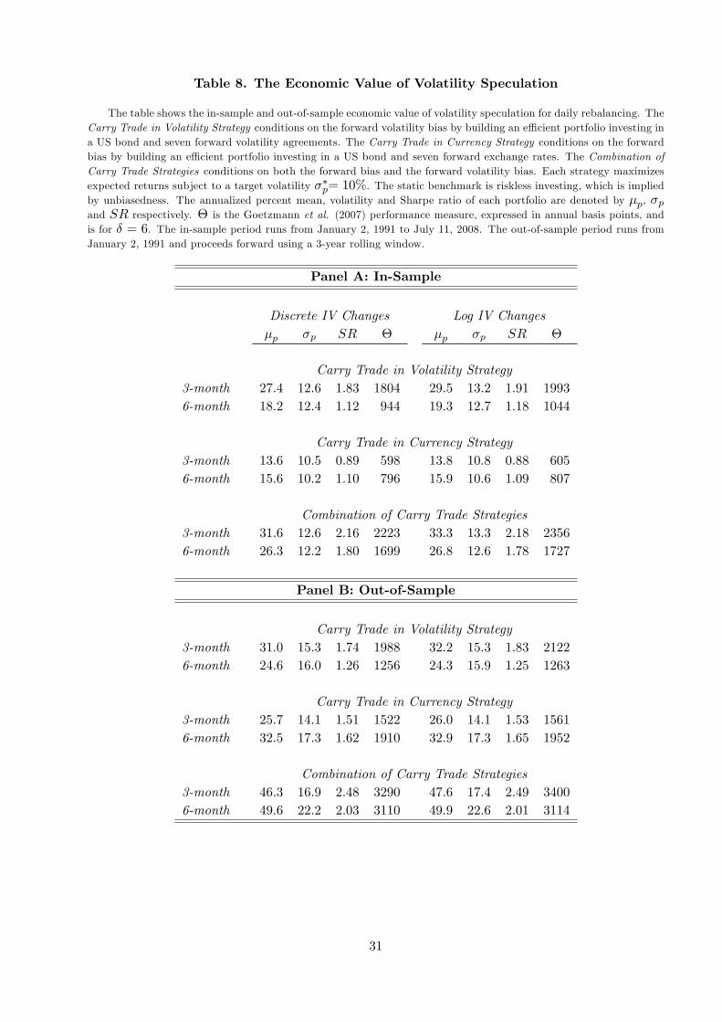
Table 8. The Economic Value of Volatility Speculation

The table shows the in-sample and out-of-sample economic value of volatility speculation for daily rebalancing. TheCarry Trade in Volatility Strategy conditions on the forward volatility bias by building an e¢ cient portfolio investing ina US bond and seven forward volatility agreements. The Carry Trade in Currency Strategy conditions on the forwardbias by building an e¢ cient portfolio investing in a US bond and seven forward exchange rates. The Combination ofCarry Trade Strategies conditions on both the forward bias and the forward volatility bias. Each strategy maximizesexpected returns subject to a target volatility ��p= 10%. The static benchmark is riskless investing, which is impliedby unbiasedness. The annualized percent mean, volatility and Sharpe ratio of each portfolio are denoted by �p, �pand SR respectively. � is the Goetzmann et al. (2007) performance measure, expressed in annual basis points, andis for � = 6. The in-sample period runs from January 2, 1991 to July 11, 2008. The out-of-sample period runs fromJanuary 2, 1991 and proceeds forward using a 3-year rolling window.

Panel A: In-Sample

Discrete IV Changes Log IV Changes�p �p SR � �p �p SR �

Carry Trade in Volatility Strategy3-month 27:4 12:6 1:83 1804 29:5 13:2 1:91 1993

6-month 18:2 12:4 1:12 944 19:3 12:7 1:18 1044

Carry Trade in Currency Strategy3-month 13:6 10:5 0:89 598 13:8 10:8 0:88 605

6-month 15:6 10:2 1:10 796 15:9 10:6 1:09 807

Combination of Carry Trade Strategies3-month 31:6 12:6 2:16 2223 33:3 13:3 2:18 2356

6-month 26:3 12:2 1:80 1699 26:8 12:6 1:78 1727

Panel B: Out-of-Sample

Carry Trade in Volatility Strategy3-month 31:0 15:3 1:74 1988 32:2 15:3 1:83 2122

6-month 24:6 16:0 1:26 1256 24:3 15:9 1:25 1263

Carry Trade in Currency Strategy3-month 25:7 14:1 1:51 1522 26:0 14:1 1:53 1561

6-month 32:5 17:3 1:62 1910 32:9 17:3 1:65 1952

Combination of Carry Trade Strategies3-month 46:3 16:9 2:48 3290 47:6 17:4 2:49 3400

6-month 49:6 22:2 2:03 3110 49:9 22:6 2:01 3114

31

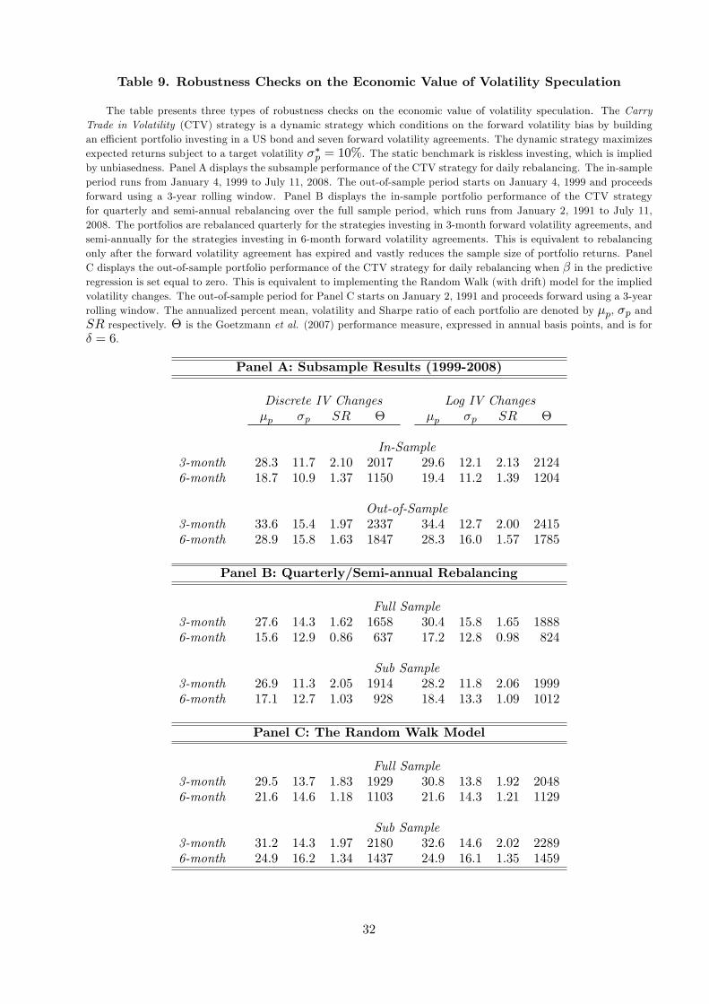
Table 9. Robustness Checks on the Economic Value of Volatility Speculation

The table presents three types of robustness checks on the economic value of volatility speculation. The CarryTrade in Volatility (CTV) strategy is a dynamic strategy which conditions on the forward volatility bias by buildingan e¢ cient portfolio investing in a US bond and seven forward volatility agreements. The dynamic strategy maximizesexpected returns subject to a target volatility ��p = 10%. The static benchmark is riskless investing, which is impliedby unbiasedness. Panel A displays the subsample performance of the CTV strategy for daily rebalancing. The in-sampleperiod runs from January 4, 1999 to July 11, 2008. The out-of-sample period starts on January 4, 1999 and proceedsforward using a 3-year rolling window. Panel B displays the in-sample portfolio performance of the CTV strategyfor quarterly and semi-annual rebalancing over the full sample period, which runs from January 2, 1991 to July 11,2008. The portfolios are rebalanced quarterly for the strategies investing in 3-month forward volatility agreements, andsemi-annually for the strategies investing in 6-month forward volatility agreements. This is equivalent to rebalancingonly after the forward volatility agreement has expired and vastly reduces the sample size of portfolio returns. PanelC displays the out-of-sample portfolio performance of the CTV strategy for daily rebalancing when � in the predictiveregression is set equal to zero. This is equivalent to implementing the Random Walk (with drift) model for the impliedvolatility changes. The out-of-sample period for Panel C starts on January 2, 1991 and proceeds forward using a 3-yearrolling window. The annualized percent mean, volatility and Sharpe ratio of each portfolio are denoted by �p, �p andSR respectively. � is the Goetzmann et al. (2007) performance measure, expressed in annual basis points, and is for� = 6.

Panel A: Subsample Results (1999-2008)

Discrete IV Changes Log IV Changes�p �p SR � �p �p SR �

In-Sample3-month 28:3 11:7 2:10 2017 29:6 12:1 2:13 21246-month 18:7 10:9 1:37 1150 19:4 11:2 1:39 1204

Out-of-Sample3-month 33:6 15:4 1:97 2337 34:4 12:7 2:00 24156-month 28:9 15:8 1:63 1847 28:3 16:0 1:57 1785

Panel B: Quarterly/Semi-annual Rebalancing

Full Sample3-month 27:6 14:3 1:62 1658 30:4 15:8 1:65 18886-month 15:6 12:9 0:86 637 17:2 12:8 0:98 824

Sub Sample3-month 26:9 11:3 2:05 1914 28:2 11:8 2:06 19996-month 17:1 12:7 1:03 928 18:4 13:3 1:09 1012

Panel C: The Random Walk Model

Full Sample3-month 29:5 13:7 1:83 1929 30:8 13:8 1:92 20486-month 21:6 14:6 1:18 1103 21:6 14:3 1:21 1129

Sub Sample3-month 31:2 14:3 1:97 2180 32:6 14:6 2:02 22896-month 24:9 16:2 1:34 1437 24:9 16:1 1:35 1459

32

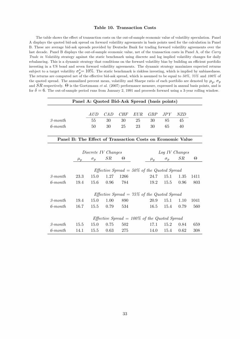
Table 10. Transaction Costs

The table shows the e¤ect of transaction costs on the out-of-sample economic value of volatility speculation. PanelA displays the quoted bid-ask spread on forward volatility agreements in basis points used for the calculation in PanelB. These are average bid-ask spreads provided by Deutsche Bank for trading forward volatility agreements over thelast decade. Panel B displays the out-of-sample economic value, net of the transaction costs in Panel A, of the CarryTrade in Volatility strategy against the static benchmark using discrete and log implied volatility changes for dailyrebalancing. This is a dynamic strategy that conditions on the forward volatility bias by building an e¢ cient portfolioinvesting in a US bond and seven forward volatility agreements. The dynamic strategy maximizes expected returnssubject to a target volatility ��p= 10%. The static benchmark is riskless investing, which is implied by unbiasedness.The returns are computed net of the e¤ective bid-ask spread, which is assumed to be equal to 50%, 75% and 100% ofthe quoted spread. The annualized percent mean, volatility and Sharpe ratio of each portfolio are denoted by �p, �pand SR respectively. � is the Goetzmann et al. (2007) performance measure, expressed in annual basis points, and isfor � = 6. The out-of-sample period runs from January 2, 1991 and proceeds forward using a 3-year rolling window.

Panel A: Quoted Bid-Ask Spread (basis points)

AUD CAD CHF EUR GBP JPY NZD3-month 55 30 30 25 30 85 45

6-month 50 30 25 23 30 65 40

Panel B: The E¤ect of Transaction Costs on Economic Value

Discrete IV Changes Log IV Changes�p �p SR � �p �p SR �

E¤ective Spread = 50% of the Quoted Spread3-month 23:3 15:0 1:27 1266 24:7 15:1 1:35 1411

6-month 19:4 15:6 0:96 784 19:2 15:5 0:96 803

E¤ective Spread = 75% of the Quoted Spread3-month 19:4 15:0 1:00 890 20:9 15:1 1:10 1041

6-month 16:7 15:5 0:79 534 16:5 15:4 0:79 560

E¤ective Spread = 100% of the Quoted Spread3-month 15:5 15:0 0:75 502 17:1 15:2 0:84 659

6-month 14:1 15:5 0:63 275 14:0 15:4 0:62 308

33

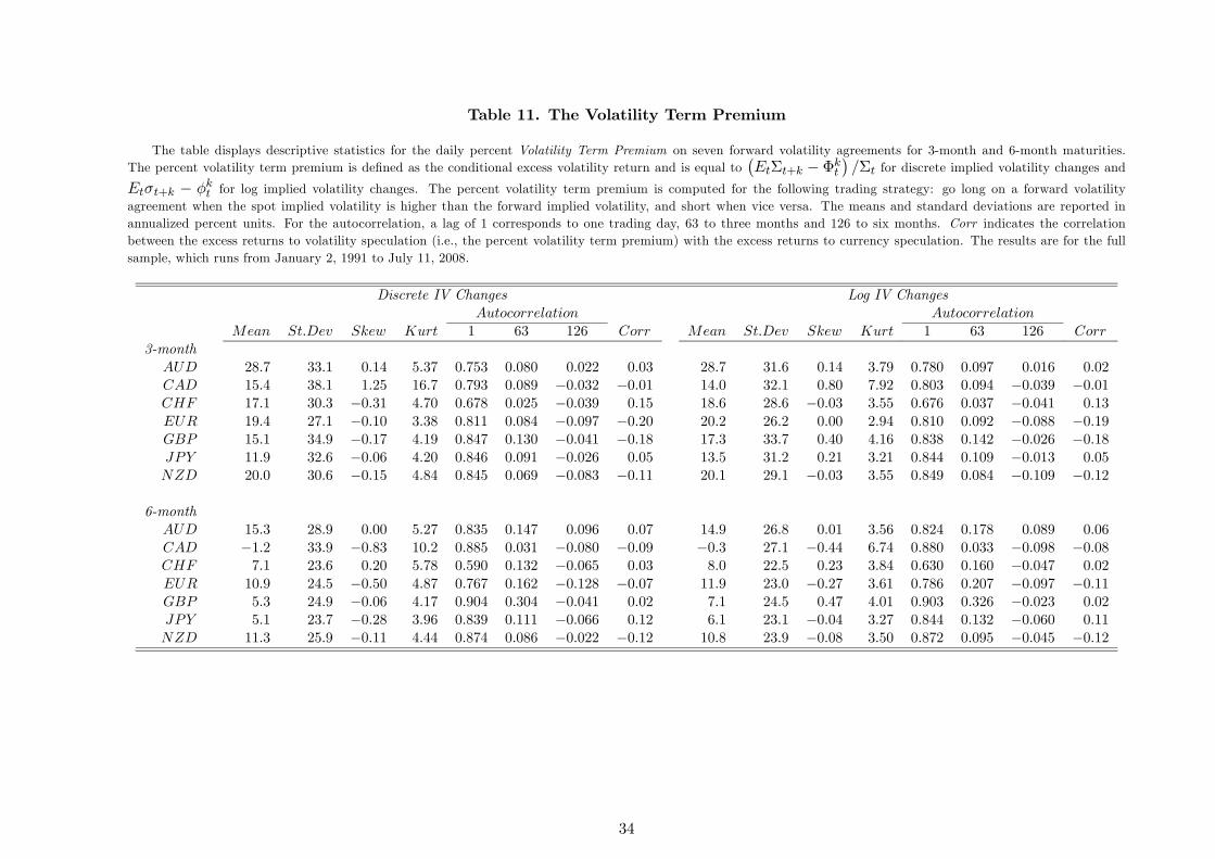
Table 11. The Volatility Term Premium

The table displays descriptive statistics for the daily percent Volatility Term Premium on seven forward volatility agreements for 3-month and 6-month maturities.The percent volatility term premium is defined as the conditional excess volatility return and is equal to

¡EtΣt+k −Φkt

¢/Σt for discrete implied volatility changes and

Etσt+k − φkt for log implied volatility changes. The percent volatility term premium is computed for the following trading strategy: go long on a forward volatilityagreement when the spot implied volatility is higher than the forward implied volatility, and short when vice versa. The means and standard deviations are reported inannualized percent units. For the autocorrelation, a lag of 1 corresponds to one trading day, 63 to three months and 126 to six months. Corr indicates the correlationbetween the excess returns to volatility speculation (i.e., the percent volatility term premium) with the excess returns to currency speculation. The results are for the fullsample, which runs from January 2, 1991 to July 11, 2008.

Discrete IV Changes Log IV ChangesAutocorrelation Autocorrelation

Mean St.Dev Skew Kurt 1 63 126 Corr Mean St.Dev Skew Kurt 1 63 126 Corr3-month

AUD 28.7 33.1 0.14 5.37 0.753 0.080 0.022 0.03 28.7 31.6 0.14 3.79 0.780 0.097 0.016 0.02CAD 15.4 38.1 1.25 16.7 0.793 0.089 −0.032 −0.01 14.0 32.1 0.80 7.92 0.803 0.094 −0.039 −0.01CHF 17.1 30.3 −0.31 4.70 0.678 0.025 −0.039 0.15 18.6 28.6 −0.03 3.55 0.676 0.037 −0.041 0.13

EUR 19.4 27.1 −0.10 3.38 0.811 0.084 −0.097 −0.20 20.2 26.2 0.00 2.94 0.810 0.092 −0.088 −0.19GBP 15.1 34.9 −0.17 4.19 0.847 0.130 −0.041 −0.18 17.3 33.7 0.40 4.16 0.838 0.142 −0.026 −0.18JPY 11.9 32.6 −0.06 4.20 0.846 0.091 −0.026 0.05 13.5 31.2 0.21 3.21 0.844 0.109 −0.013 0.05NZD 20.0 30.6 −0.15 4.84 0.845 0.069 −0.083 −0.11 20.1 29.1 −0.03 3.55 0.849 0.084 −0.109 −0.12

6-monthAUD 15.3 28.9 0.00 5.27 0.835 0.147 0.096 0.07 14.9 26.8 0.01 3.56 0.824 0.178 0.089 0.06CAD −1.2 33.9 −0.83 10.2 0.885 0.031 −0.080 −0.09 −0.3 27.1 −0.44 6.74 0.880 0.033 −0.098 −0.08CHF 7.1 23.6 0.20 5.78 0.590 0.132 −0.065 0.03 8.0 22.5 0.23 3.84 0.630 0.160 −0.047 0.02

EUR 10.9 24.5 −0.50 4.87 0.767 0.162 −0.128 −0.07 11.9 23.0 −0.27 3.61 0.786 0.207 −0.097 −0.11GBP 5.3 24.9 −0.06 4.17 0.904 0.304 −0.041 0.02 7.1 24.5 0.47 4.01 0.903 0.326 −0.023 0.02JPY 5.1 23.7 −0.28 3.96 0.839 0.111 −0.066 0.12 6.1 23.1 −0.04 3.27 0.844 0.132 −0.060 0.11NZD 11.3 25.9 −0.11 4.44 0.874 0.086 −0.022 −0.12 10.8 23.9 −0.08 3.50 0.872 0.095 −0.045 −0.12

34

Fig

ure

1.Spot

and

For

war

dIm

plied

Vol

atilitie

s

The

figure

dis

pla

ys

the

daily

3-m

onth

ahea

dsp

ot

and

forw

ard

implied

vola

tiliti

esin

annualize

dp

erce

nt

unit

son

seven

exch

ange

rate

svis

-a-v

isth

eU

Sdollar.

35

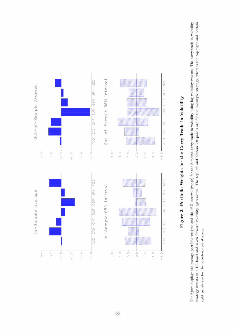
Fig

ure

2.Por

tfol

ioW

eigh

tsfo

rth

eC

arry

Tra

de

inV

olat

ility

The

figure

dis

pla

ys

the

aver

age

port

folio

wei

ghts

and

the

95%

inte

rval

(range)

for

the

3-m

onth

carr

ytr

ade

invola

tility

usi

ng

log

vola

tility

retu

rns.

The

carr

ytr

ade

invola

tility

stra

tegy

inves

tsin

aU

Sb

ond

and

seven

forw

ard

vola

tility

agre

emen

ts.

The

top

left

and

bott

om

left

panel

sare

for

the

in-s

am

ple

stra

tegy,

wher

eas

the

top

right

and

bott

om

right

panel

sare

for

the

out-

of-

sam

ple

stra

tegy.

36

Figure 3. Rolling Out-of-Sample Sharpe Ratios

The figure displays the rolling out-of-sample annualized Sharpe Ratio for the carry trade in volatility and the carry trade

in currency. The rolling Sharpe Ratio is computed using a three-year rolling window on log volatility returns. The carry

trade in volatility strategy invests in a US bond and seven forward volatility agreements. The carry trade in currency

strategy invests in a US bond and seven forward exchange rates. The top panel shows the strategies for a 3-month

maturity. The bottom panel shows the strategies for a 6-month maturity.

37

References

Ang, A., R.J. Hodrick, Y. Xing, and X. Zhang (2006). �The Cross-Section of Volatility and ExpectedReturns,�Journal of Finance 61, 259�299.

Backus, D.K., S. Foresi, and C.I. Telmer (2001). �A¢ ne Term Structure Models and the ForwardPremium Anomaly,�Journal of Finance 56, 279�304.

Backus, D.K., A.W. Gregory, and C.I. Telmer (1993). �Accounting for Forward Rates in Markets forForeign Currency,�Journal of Finance 48, 1887�1908.

Bakshi, G., P. Carr, and L. Wu (2008). �Stochastic Risk Premiums, Stochastic Skewness in Cur-rency Options, and Stochastic Discount Factors in International Economies,�Journal of FinancialEconomics 87, 132�156.

Bakshi, G., and N. Kapadia (2003). �Delta-Hedged Gains and the Negative Market Volatility RiskPremium,�Review of Financial Studies 16, 527�566.

Bakshi, G., and D. Madan (2006). �A Theory of Volatility Spreads,�Management Science 52, 1945�1956.

Bank for International Settlements (2007). �Triennial Central Bank Survey of Foreign Exchange andDerivatives Market Activity in 2007.�

Bansal, R. (1997). �An Exploration of the Forward Premium Puzzle in Currency Markets,�Reviewof Financial Studies 10, 369�403.

Bassett, G., and R. Koenker (1978). �Asymptotic Theory of Least Absolute Error Regression,�Journal of the American Statistical Association 73, 618�622.

Battalio, R.H., B. Hatch, and R. Jennings (2004). �Toward a National Market System for U.S.Exchange-Listed Equity Options,�Journal of Finance 59, 933�962.

Bates, D.S. (2008). �The Market for Crash Risk,�Journal of Economic Dynamics and Control 32,2291�2321.

Bekaert, G. (1996). �The Time-Variation of Risk and Return in Foreign Exchange Markets: AGeneral Equilibrium Perspective,�Review of Financial Studies 9, 427�470.

Bekaert, G., and R.J. Hodrick (2001). �Expectations Hypotheses Tests,� Journal of Finance 56,115�138.

Bekaert, G., R.J. Hodrick, and D. Marshall (1997). �The Implications of First-Order Risk Aversionfor Asset Market Risk Premiums,�Journal of Monetary Economics 40, 3�39.

Berger, D., A. Chaboud, E. Hjalmarsson, and E. Howorka (2009). �What Drives Volatility Persistencein the Foreign Exchange Market?�Journal of Financial Economics (forthcoming).

Bilson, J.F.O. (1981). �The �Speculative E¢ ciency�Hypothesis,�Journal of Business 54, 435�451.

Bollerslev, T., G. Tauchen, and H. Zhou (2009). �Expected Stock Returns and Variance Risk Pre-mia,�Review of Financial Studies (forthcoming).

Britten-Jones, M., and A. Neuberger (2000). �Option Prices, Implied Price Processes, and StochasticVolatility,�Journal of Finance 55, 839�866.

38

Broadie, M., and A. Jain (2008). �Pricing and Hedging Volatility Derivatives,�Journal of Derivatives15, 7�24.

Brockhaus, O., and D. Long (2000). �Volatility Swaps Made Simple,�Risk 19, 92�95.

Brunnermeier, M.K., S. Nagel, and L.H. Pedersen (2009). �Carry Trades and Currency Crashes�NBER Macroeconomics Annual 2008, 313�347.

Burnside, C., M. Eichenbaum, I. Kleshchelski, and S. Rebelo (2008). �Do Peso Problems Explainthe Returns to the Carry Trade?�NBER Working Paper 14054.

Campa, J.M, and P.H.K. Chang (1995). �Testing the Expectations Hypothesis of the Term Structureof Volatilities in Foreign Exchange Options,�Journal of Finance 50, 529�547.

Carr, P., and L. Wu (2007). �Stochastic Skew in Currency Options,�Journal of Financial Economics86, 213�247.

Carr, P., and L. Wu (2009). �Variance Risk Premiums,�Review of Financial Studies 22, 1311�1341.

Christensen, B.J., and N.R. Prabhala (1998). �The Relation between Implied and Realized Volatil-ity,�Journal of Financial Economics 50, 125�150.

Coval, J.D., and T. Shumway (2001). �Expected Option Returns,�Journal of Finance 56, 983�1009.

De Fontnouvelle, P., R.P.H. Fishe, and J.H. Harris (2003). �The Behavior of Bid�Ask Spreads andVolume in Options Markets during the Competition for Listings in 1999,� Journal of Finance 58,2437�2464.

Della Corte, P., L. Sarno, and D.L. Thornton (2008). �The Expectation Hypothesis of the TermStructure of very Short-Term Rates: Statistical Tests and Economic Value,� Journal of FinancialEconomics 89, 158�174.

Della Corte, P., L. Sarno, and I. Tsiakas (2009). �An Economic Evaluation of Empirical ExchangeRate Models.�Review of Financial Studies 22, 3491�3530.

Detemer�, K., E. Derman, M. Kamal, and J. Zou (1999). �A Guide to Volatility and VarianceSwaps,�Journal of Derivatives 6, 9�32.

Driessen, J., P. Maenhout, and G. Vilkov (2009). �The Price of Correlation Risk: Evidence fromEquity Options,�Journal of Finance 64, 1377�1406.

Duarte, J., and C.S. Jones (2007). �The Price of Market Volatility Risk,�Working Paper, Universityof Southern California.

Engel, C. (1996). �The Forward Discount Anomaly and the Risk Premium: A Survey of RecentEvidence,�Journal of Empirical Finance 3, 123�192.

Fama, E.F. (1984). �Forward and Spot Exchange Rates,�Journal of Monetary Economics 14, 319�338.

Farhi, E., S.P. Fraiberger, X. Gabaix, R. Ranciere, and A. Verdelhan (2009). �Crash Risk in CurrencyMarkets,�NBER Working Paper 15062.

Fleming, J., C. Kirby, and B. Ostdiek (2001). �The Economic Value of Volatility Timing,�Journalof Finance 56, 329�352.

39

Galati, G., and M. Melvin (2004). �Why Has FX Trading Surged? Explaining the 2004 TriennialSurvey,�BIS Quarterly Review, December, 67�74.

Gatheral, J. (2006). The Volatility Surface: A Practitioner�s Guide, New York: Wiley.

Goetzmann, W., J. Ingersoll, M. Spiegel, and I. Welch (2007). �Portfolio Performance Manipulationand Manipulation-Proof Performance Measures,�Review of Financial Studies 20, 1503�1546.

Goyal, A., and A. Saretto (2009). �Cross-Section of Option Returns and Volatility,� Journal ofFinancial Economics (forthcoming).

Han, Y. (2006). �Asset Allocation with a High Dimensional Latent Factor Stochastic VolatilityModel,�Review of Financial Studies 19, 237�271.

Harvey, C.R., and R.E. Whaley (1991). �S&P 100 Index Option Volatility,�Journal of Finance 46,1551�1561.

Harvey, C.R., and R.E. Whaley (1992). �Market Volatility Prediction and the E¢ ciency of the S&P100 Index Option Market,�Journal of Financial Economics 31, 43�73.

Hodrick, R.J. (1987). The Empirical Evidence on the E¢ ciency of Forward and Futures ForeignExchange Markets, London: Harwood.

Hodrick, R.J., and S. Srivastava (1984). �An Investigation of Risk and Return in Foreign Exchange,�Journal of International Money and Finance 3, 5�29.

Jiang, G.J., and Y.S. Tian (2005). �The Model-Free Implied Volatility and Its Information Content,�Review of Financial Studies 18, 1305�1342.

Jorion, P. (1995). �Predicting Volatility in the Foreign Exchange Market,�Journal of Finance 50,507�528.

Kandel, S., and R.F. Stambaugh (1996). �On the Predictability of Stock Returns: An Asset-Allocation Perspective,�Journal of Finance 51, 385�424.

Kim, M., and M. Kim (2003). �Implied Volatility Dynamics in the Foreign Exchange Markets,�Journal of International Money and Finance 22, 511�528.

Knauf, S. (2003). �Making Money from FX Volatility,�Quantitative Finance 3, 48�51.

Krishnan, C.N.V., R. Petkova, and P. Ritchken (2009). �Correlation Risk,� Journal of EmpiricalFinance 16, 353�367.

Low, B.S., and S. Zhang (2005). �The Volatility Risk Premium Embedded in Currency Options,�Journal of Financial and Quantitative Analysis 40, 803�832.

Lustig, H., and A. Verdelhan (2007). �The Cross-Section of Currency Risk Premia and US Consump-tion Growth Risk,�American Economic Review 97, 89�117.

Marquering, W., and M. Verbeek (2004). �The Economic Value of Predicting Stock Index Returnsand Volatility,�Journal of Financial and Quantitative Analysis 39, 407�429.

Mayhew, S. (2002). �Competition, Market Structure, and Bid-Ask Spreads in Stock Option Markets,�Journal of Finance 57, 931�958.

Meese, R.A., and K. Rogo¤ (1983). �Empirical Exchange Rate Models of the Seventies: Do TheyFit Out of Sample?�Journal of International Economics 14, 3�24.

40

Neuberger, A. (1994). �The Log Contract: A New Instrument to Hedge Volatility,� Journal ofPortfolio Management 20, 74�80.

Newey, W.K., and K.D. West (1987). �A Simple, Positive Semi-De�nite, Heteroskedasticity andAutocorrelation Consistent Covariance Matrix,�Econometrica 55, 703�708.

Poon, S.-H., and C. Granger (2003). �Forecasting Volatility in Financial Markets: A Review,�Journalof Economic Literature 41, 478�539.

Poterba, J.M., and L.H. Summers (1986). �The Persistence of Volatility and Stock Market Fluctua-tions,�American Economic Review 76, 1142�1151.

Sarno, L. (2005). �Towards a Solution to the Puzzles in Exchange Rate Economics: Where Do WeStand?�Canadian Journal of Economics 38, 673�708.

Siegel, J.J. (1972). �Risk, Interest Rates and the Forward Exchange,�Quarterly Journal of Economics86, 303�309.

Stein, J. (1989). �Overreactions in the Options Market,�Journal of Finance 44, 1011�1023.

Verdelhan, A. (2009). �A Habit-Based Explanation of the Exchange Rate Risk Premium,�Journalof Finance (forthcoming).

Weiss, A.A. (1990). �Least Absolute Error Estimation in the Presence of Serial Correlation,�Journalof Econometrics 44, 127�158.

West, K.D., H.J. Edison, and D. Cho (1993). �A Utility-Based Comparison of Some Models ofExchange Rate Volatility,�Journal of International Economics 35, 23�45.

Windcli¤, H., P.A. Forsyth, and K.R. Vetzal (2006). �Pricing Methods and Hedging Strategies forVolatility Derivatives,�Journal of Banking and Finance 30, 409�431.

41