An investigation of induced drag minimization using a …oddjob.utias.utoronto.ca/dwz/Miscellaneous/HZ_aiaa_opt_MDO_2008.pdf · An investigation of induced drag minimization ... The

An investigation of induced drag minimization

using a Newton-Krylov algorithm

Jason E. Hicken∗ and David W. Zingg †

Institute for Aerospace Studies, University of Toronto, Toronto, Ontario, M3H 5T6, Canada

We present an optimization algorithm for the study of induced drag minimization, with

applications to unconventional aircraft design. The algorithm is based on a discrete-adjoint

formulation and uses an efficient parallel-Newton-Krylov solution strategy. We validate the

optimizer by recovering an elliptical lift distribution using twist optimization; we believe

this an important, and under-appreciated, benchmark for aerodynamic optimization. The

algorithm is further illustrated using several design examples, including planform, spanwise

vertical shape, and box-wing optimization.

I. Introduction

The aircraft industry faces two challenges in the twenty-first century: climate change and peak oilproduction. These problems may eventually be solved by alternative fuels such as hydrogen, bio-kerosene,and coal-based kerosene (provided that carbon from the coal is sequestered); however, when productionemissions are included, these alternative fuels presently produce more greenhouse gases than traditionalkerosene.1 Alternative fuels must, therefore, be considered a long term solution.

In the near term, reduced emissions and improved fuel efficiency may be possible by considering un-conventional configurations, such as the often cited blended-wing-body; see, for example, Liebeck.2 Theevolution of the blended-wing-body concept and advent of aerodynamic shape optimization motivate the fol-lowing question: can we use numerical optimization to “discover” radically new concepts in aircraft design?In this paper we present an algorithm which we hope can begin addressing this question.

Our preliminary goal is to develop an Euler-based optimization code capable of minimizing induced drag.While viscous and turbulence effects cannot be neglected in practical applications, it is important that theoptimizer accurately minimize drag due to lift. This requirement can be motivated by considering a typicalcommercial aircraft, where induced drag represents 40% of the total drag.3

In addition to presenting the optimization algorithm, we hope to shed some light on a useful, but over-looked, benchmark for aerodynamic optimization. An elliptical lift distribution is known to minimize induceddrag for planar configurations at low Mach numbers. Recovering an elliptical distribution as a (local) opti-mum should be a reasonable validation for any aerodynamic optimization algorithm; nevertheless, we havefound no evidence in the literature that such a benchmark has ever been used explicitly for Euler-basedoptimizations.

Broadly, the paper is divided into a description of the algorithm and its illustration with examples. Thealgorithm description, Sections II–IV, follows the sequence of operations as they would be encountered in atypical design iteration. In particular, Section II describes the design space parametrization and integratedmesh movement algorithm. Subsequently, Section III reviews the Euler flow solver used for analysis. Gradientevaluation is covered in Section IV, including details regarding the flow and mesh adjoint equations. Thesecond half of the paper includes verification and validation, presented in Section V, and design examples,provided in Section VI. A summary and our conclusions are given in Section VII

∗PhD Candidate, AIAA Student Member†Professor and Director, Tier 1 Canada Research Chair in Computational Aerodynamics, Associate Fellow AIAA

1 of 19

American Institute of Aeronautics and Astronautics

II. Design Parametrization and Mesh Movement

The choice of parametrization places implicit constraints on the design space. The design variables shouldbe sufficiently powerful, in the sense of approximation theory, to minimize the effects of these constraints.In turn, the mesh movement algorithm should be capable of accepting any geometrically physical designproduced by the parametrization. For the present work, we use the control points from B-spline meshes forboth parametrization and mesh movement. The complete details of the this integrated approach are givenin a companion paper.4 We provide only a brief outline of the method below.

A. B-spline Meshes

Consider a B-spline tensor product volume mapping the cubic computational domain D = {ξ = (ξ, η, ζ) ∈R

3|ξ, η, ζ ∈ [0, 1]} to the physical domain P ∈ R3:

x(ξ) =

Ni∑

i=1

Nj∑

j=1

Nk∑

k=1

BijkNi(ξ; η, ζ)Nj(η; ζ, ξ)Nk(ζ; ξ, η). (1)

The set of points {Bijk} defines the control mesh which can be used to manipulate the volume. The functionsNi, Nj , and Nk, described below, are the modified B-spline basis functions. A B-spline mesh is obtained bydiscretizing the cubic domain D.

The basis functions Ni, Nj , and Nk are modified versions of the standard B-spline basis; for definitionsof the standard basis see de Boor.5 The modified bases differ in that they use spatially varying knot vectors,also called curved knot lines.6 For example, the knots defining Ni(ξ; η, ζ) are bilinear functions of η andζ; hence, for fixed (η, ζ) the function Ni(ξ; η, ζ) reduces to the standard basis. The spatially varying knotvectors permit better approximations of the initial grid and geometry.

Suppose an initial design surface is given, together with a conforming computational mesh. A prepro-cessing stage approximates each block of the grid using B-spline volumes. The approximation algorithmis based on the parameter correction method proposed by Hoschek.7 The initial (ξ, η, ζ) parameters andknot vectors are given a chord length spacing, which produces a control mesh that mimics a coarse grid.Thus, the control points corresponding to the surface patches provide a low dimensional approximation ofthe design. Bezier or B-spline control points have been used as design variables by many authors; see, forexample, Burgreen and Baysal8 or Nemec et al.;9 the difference here is that the design variables are a subsetof a volume control mesh.

To formalize the design variable definition, let b be a block column vector of all control points. Further-more, let b be ordered such that all internal control points are first, then non-surface boundary points, andfinally the Ns surface control points. The vector of (geometric) design variables is defined by the restrictionoperation

v ≡[

0 0 I]

b (2)

where I is the 3Ns × 3Ns identity matrix.

B. Semi-Algebraic Mesh Movement

When the geometric design variables change, the mesh must be updated to conform to the new surface.Here, the surface control points are the design variables, so the surface mesh automatically conforms to thedesign. Moreover, by moving the internal control points in response to the surface control points, we canmaintain the quality of the volume grid.

As noted above, the control mesh obtained by fitting the initial grid is a coarse approximation of theactual mesh. By applying different mesh movement algorithms to the control points, rather than the grid, afamily of mesh movement algorithms is possible. For example, we use a linear elasticity algorithm, describedby Truong et al.,10 to perturb the internal control mesh based on the surface control points. Subsequently,the fine grid is regenerated algebraically using equation (1).

We briefly describe the mesh movement algorithm of Truong et al.10 to help elucidate the details of thegradient calculation in Section IV. The algorithm breaks the movement into m equal increments to improverobustness — the linear elasticity equation assumes small displacements. The residual vectors, obtained

2 of 19


from a trilinear finite-element discretization of the governing equations, are

M(i)(

b(i),b(i−1))

= K(i)(

b(i−1)) [

b(i) − b(i−1)]

− f (i) = 0, i = 1, . . . , m. (3)

In the above equation, b(i) is the vector of B-spline control points at increment stage i, and f (i) is the vectorof forces. The forces are defined implicitly to account for the boundary movement. The stiffness matrix K(i)

is symmetric positive definite with respect to the unknown degrees of freedom; thus, we use the conjugategradient method with ILU(p)11 preconditioning to solve (3) for each increment i. These equations can beexpensive to solve when applied to the actual computational mesh; however, since the control mesh has 2 to3 orders fewer degrees of freedom, solutions to (3) are obtained in negligible time relative to the flow solver.For example, consider a 12 block mesh fitted using 9×9×9 control points per block. Then solving equations(3) with m = 5, to a relative tolerance of 10−12, requires 128 seconds on a 1500 MHz Itanium 2 processor.

Notice that the stiffness matrix in (3) is a function of the B-spline control points at the previous increment.This functional dependence arises because the Young’s modulus is assumed to depend on the control meshcell volumes and quality. In other words, for each control mesh element E we have

E(i)E

= E(i)E

(b(i−1)).

This (nonlinear) dependence on the previous increment is important to consider when differentiating themesh movement algorithm.

We now summarize the design parametrization and mesh movement. The grid around an initial designis approximated using B-spline volumes. The coordinates of the surface control points become the designvariables. When the design changes, the internal control points are updated using linear elasticity, and thegrid is regenerated algebraically.

III. Flow Analysis

The flow solver incorporated into the optimization algorithm uses a second-order accurate finite-differencediscretization and a Newton-Krylov solution strategy. The solver is described briefly below, and in detail inreference 12.

A. Governing Equations and Discretization

In this study we consider the 3-dimensional Euler equations on multi-block structured grids. Applying adiffeomorphism from physical to computational space, the Euler equations become

∂tQ + ∂ξiEi = 0, (4)

where ξ = (ξ1, ξ2, ξ3) = (ξ, η, ζ),

Q =1

J

ρ

ρu1

ρu2

ρu3

e

, and Ei =1

J

ρUi

ρu1Ui + p∂xξi

ρu2Ui + p∂yξi

ρu3Ui + p∂zξi

(e + p)Ui

.

The scalar J denotes the Jacobian of the mapping, and the Ui are the contravariant velocities defined byUi = uj∂xj

ξi.The convective fluxes in (4) are discretized using second-order accurate summation-by-parts (SBP) oper-

ators.13 Boundary conditions are imposed and blocks are coupled using simultaneous approximation terms(SATs).14 The SBP-SAT discretization is linearly time-stable, requires only C0 mesh continuity at blockinterfaces, accommodates arbitrary block topologies, and has low inter-block communication overhead. Tosuppress high frequency modes, the discretization is augmented with scalar dissipation,15, 16 and, in somecases, with matrix dissipation.17 The resulting nonlinear set of algebraic equations is represented by thevector equation

F(q) = 0, (5)

where q is a block column vector of the conservative flow variables.

3 of 19


B. Inexact-Newton Algorithm

We solve the discretized Euler equations using a Newton-Krylov strategy. Applying Newton’s method to (5)produces the following linear update for each Newton (outer) iteration n:

A(n)∆q(n) = −F(n), (6)

where F(n) = F(qn), ∆q(n) = q(n+1) − q(n), and

A(n)ij =

∂Fi

∂qj

(

q(n))

.

Successful convergence of Newton’s method depends on the initial iterate, q(0), which must be sufficientlyclose to the solution of (5).18 For this reason, our solution algorithm is broken into two phases: 1) a start-upphase to find a suitable “initial” iterate, and; 2) an inexact-Newton phase. We describe these phases below,starting with the second.

The inexact-Newton phase gets its name from solving (6) inexactly with, for example, a Krylov linearsolver. This strategy is useful, because an inexpensive inexact-Newton update may reduce the nonlinearresidual by the same magnitude as the exact update. In addition, Krylov solvers do not need the Jacobianmatrix explicitly; they only need Jacobian-vector products of the form A(n)z. This matrix-vector productcan be calculated to first-order with the forward-difference equation

A(n)z ≈F(qn + ǫz) − F(qn)

ǫ. (7)

The perturbation parameter must be chosen carefully to minimize truncation error and avoid round-offerrors.19 We use a perturbation suggested by Nielsen et al.:20

ǫ =

√

Nδ

zT z,

where δ = 10−13 and N is the number of unknowns.The start-up phase is invoked to find an initial iterate for the inexact-Newton phase. The start-up phase

is similar to the implicit Euler method with some important modifications which we now describe. Thetime step varies spatially with mesh spacing to roughly approximate a constant CFL.16 The Jacobian A(n)

is replaced with a first-order approximation obtained by lumping the fourth-difference dissipation into thesecond-difference dissipation. This lumping reduces the stencil size and improves diagonal dominance. Duringthe start-up phase the approximate Jacobian is updated and incompletely factored every four iterations21 —factorization is used in preconditioning the linear update equation, see below. This lagged update strategyreduces factorization time while maintaining robustness.12

C. Parallel Krylov Linear System Solution

At each outer iteration of the inexact-Newton algorithm, we must solve a linear equation of the form

Ax = r. (8)

While the matrix A is different during the start-up and inexact-Newton phases, the solution strategy for thelinear equation remains the same. Specifically, we solve (8) in parallel using a preconditioned Krylov iterativemethod. Experience suggests that the generalized minimal residual method (GMRES)22 is an efficient Krylovmethod for aerodynamic applications. We use flexible GMRES (FGMRES)23 to accommodate iterativepreconditioners.

Krylov methods need to be preconditioned to be effective on ill-conditioned problems. Two parallelpreconditioners are implemented in the solver: an additive Schwarz preconditioner24, 25 with no overlap(block Jacobi), and an approximate Schur preconditioner.26 Both preconditioners require an incompletelower-upper factorization of the approximate local Jacobian matrices Ak. The matrix Ak is local because itcontains only those columns and rows corresponding to variables assigned to processor k; it is approximate,because it lumps the fourth-difference dissipation into the second-difference dissipation. ILU(p)11 with afill-level of 1 is used for the incomplete factorizations.

4 of 19


IV. Lagrangian Formulation and Gradient Evaluation

Let J denote an objective function that we wish to minimize; for example, drag or CD/CL. We requirethat a valid optimal point satisfy the mesh movement and flow equations; therefore, the optimization problemcan be posed mathematically as follows:

min J(

q,b(m),v)

(9)

w.r.t. q,b(m),v,

s.t. M(i)(

b(i),b(i−1))

= 0, i ∈ {1, 2, . . . , m}

F

(

q,b(m))

= 0

Recall that v are the design variables, b(i) are the B-spline control points, and q are the flow variables.Following the standard approach, we introduce the Lagrangian function, L, for the constrained optimiza-

tion problem (9):

L = J +

m∑

i=1

λ(i)T

M(i) +ψT

F . (10)

The Lagrange multipliers λ(i) and ψ are the mesh and flow adjoint variables, respectively. The first-order(necessary) optimality conditions for the problem (9) are obtained by setting the partial derivatives of L tozero:27

∂L

∂λ(i)= 0 = M

(i), i ∈ {1, 2, . . . , m} (11)

∂L

∂ψ= 0 = F (12)

∂L

∂q= 0 =

∂J

∂q+ψT ∂F

∂q(13)

∂L

∂b(m)= 0 =

∂J

∂b(m)+ λ(i)T ∂M

(m)

∂b(m)+ψT ∂F

∂b(m)(14)

∂L

∂b(i)= 0 = λ(i)T ∂M

(i)

∂b(i)+ λ(i+1)T ∂M

(i+1)

∂b(i), i ∈ {m − 1, m − 2, . . . , 1} (15)

∂L

∂v= 0 =

∂J

∂v+

m∑

i=1

(

λ(i)T ∂M(i)

∂b(i)

∂b(i)

∂v

)

+ψT ∂F

∂v(16)

The optimality conditions are also called the Karush-Kuhn-Tucker (KKT) conditions.27 Note the use of abold-font notation for gradients and Jacobians; for example, (∂J/∂q)i = ∂J/∂qi. We hope this notation willclarify which terms in the KKT conditions are vectors and which are matrices.

We follow the approach outlined in Truong et al.,10 and drive the KKT conditions to zero using asequential approach. We begin with the design variables, v, which define the surface B-spline control points;see equation (2). These control points are then used as boundary conditions to solve for the control meshequations (11). Once the control mesh is determined and the mesh is generated, the flow equations (12)can be solved to find q. Subsequently, the adjoint variables can be determined using equations (13)–(15), inthat order. Finally, the gradient of the Lagrangian is calculated using (16). Using this sequential approach,all of the KKT conditions are satisfied at each step, with the exception of ∂L/∂v = 0. The gradient of theLagrangian, ∂L/∂v, is driven to zero using the sequential quadratic programming (SQP) algorithm in thesoftware SNOPT.28

A. Flow Adjoint Equation

The flow adjoint variables are governed by the linear equation

ATψ = −

(

∂J

∂q

)T

. (17)

5 of 19


Step-size

RM

SE

rror

10-2010-1510-1010-510010-17

10-15

10-13

10-11

10-9

10-7

10-5

10-3

10-1

101

complex-step

forward-difference

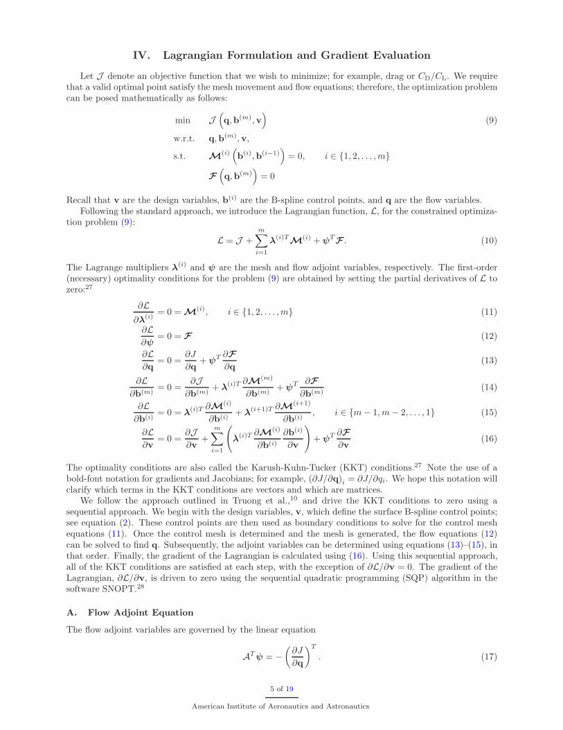
Figure 1. Verification of the analytical Jaco-

bian matrix using the complex-step method

Equivalent residual evaluations

Res

idua

lnor

m

0 1000 2000 3000 400010-8

10-7

10-6

10-5

10-4

10-3

10-2

10-1

100

FGMRES(20)

GCROT(20,0.01)

FGMRES(50)

GCROT(50,0.01)

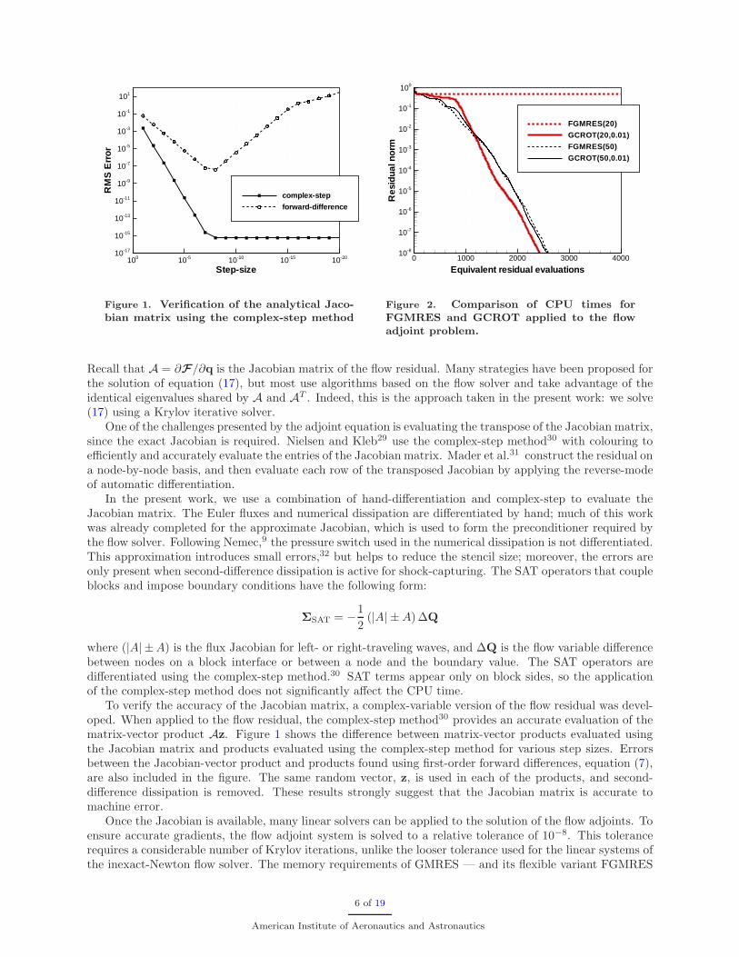
Figure 2. Comparison of CPU times for

FGMRES and GCROT applied to the flow

adjoint problem.

Recall that A = ∂F/∂q is the Jacobian matrix of the flow residual. Many strategies have been proposed forthe solution of equation (17), but most use algorithms based on the flow solver and take advantage of theidentical eigenvalues shared by A and AT . Indeed, this is the approach taken in the present work: we solve(17) using a Krylov iterative solver.

One of the challenges presented by the adjoint equation is evaluating the transpose of the Jacobian matrix,since the exact Jacobian is required. Nielsen and Kleb29 use the complex-step method30 with colouring toefficiently and accurately evaluate the entries of the Jacobian matrix. Mader et al.31 construct the residual ona node-by-node basis, and then evaluate each row of the transposed Jacobian by applying the reverse-modeof automatic differentiation.

In the present work, we use a combination of hand-differentiation and complex-step to evaluate theJacobian matrix. The Euler fluxes and numerical dissipation are differentiated by hand; much of this workwas already completed for the approximate Jacobian, which is used to form the preconditioner required bythe flow solver. Following Nemec,9 the pressure switch used in the numerical dissipation is not differentiated.This approximation introduces small errors,32 but helps to reduce the stencil size; moreover, the errors areonly present when second-difference dissipation is active for shock-capturing. The SAT operators that coupleblocks and impose boundary conditions have the following form:

ΣSAT = −1

2(|A| ± A)∆Q

where (|A| ±A) is the flux Jacobian for left- or right-traveling waves, and ∆Q is the flow variable differencebetween nodes on a block interface or between a node and the boundary value. The SAT operators aredifferentiated using the complex-step method.30 SAT terms appear only on block sides, so the applicationof the complex-step method does not significantly affect the CPU time.

To verify the accuracy of the Jacobian matrix, a complex-variable version of the flow residual was devel-oped. When applied to the flow residual, the complex-step method30 provides an accurate evaluation of thematrix-vector product Az. Figure 1 shows the difference between matrix-vector products evaluated usingthe Jacobian matrix and products evaluated using the complex-step method for various step sizes. Errorsbetween the Jacobian-vector product and products found using first-order forward differences, equation (7),are also included in the figure. The same random vector, z, is used in each of the products, and second-difference dissipation is removed. These results strongly suggest that the Jacobian matrix is accurate tomachine error.

Once the Jacobian is available, many linear solvers can be applied to the solution of the flow adjoints. Toensure accurate gradients, the flow adjoint system is solved to a relative tolerance of 10−8. This tolerancerequires a considerable number of Krylov iterations, unlike the looser tolerance used for the linear systems ofthe inexact-Newton flow solver. The memory requirements of GMRES — and its flexible variant FGMRES

6 of 19


— grow linearly with the number of iterations. This can cause problems when GMRES is applied to theadjoint problem and memory is limited. One way to reduce the memory burden is to use restarted versionsof GMRES or FGMRES, denoted GMRES(m) and FGMRES(m). These solvers simply restart after everym Krylov iterations, which keeps memory requirements proportional to m; unfortunately, restarted Krylovsolvers often exhibit degraded, and in some cases stalled, convergence.

For this work, we use a flexible variant of the Krylov method GCROT,33 preconditioned with the (trans-posed) approximate Schur preconditioner used in the flow solver. Unlike FGMRES(m), GCROT does notdiscard the entire Krylov subspace each time it restarts. Instead, it maintains a set of vectors from one outeriteration to the next based on which subspace was most important to convergence. GCROT has been shownto perform very well with respect to full GMRES while maintaining a Krylov subspace of fixed size, i.e. likeGMRES(m), memory requirements do not grow for GCROT.

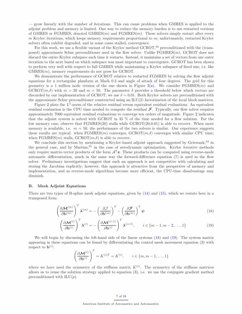
We demonstrate the performance of GCROT relative to restarted FGMRES by solving the flow adjointequations for a rectangular planform at Mach 0.3 and angle of attack of four degrees. The grid for thisgeometry is a 1 million node version of the one shown in Figure 3(a). We consider FGMRES(m) andGCROT(m,δ) with m = 20 and m = 50. The parameter δ provides a threshold below which vectors arediscarded by our implementation of GCROT; we use δ = 0.01. Both Krylov solvers are preconditioned withthe approximate Schur preconditioner constructed using an ILU(2) factorization of the local block matrices.

Figure 2 plots the L2-norm of the relative residual versus equivalent residual evaluations. An equivalentresidual evaluation is the CPU time needed to compute the residual F . Typically, our flow solver requiresapproximately 7000 equivalent residual evaluations to converge ten orders of magnitude. Figure 2 indicatesthat the adjoint system is solved with GCROT in 35 % of the time needed for a flow solution. For thelow memory case, observe that FGMRES(20) stalls while GCROT(20,0.01) is able to recover. When morememory is available, i.e. m = 50, the performance of the two solvers is similar. Our experience suggeststhese results are typical: when FGMRES(m) converges, GCROT(m,δ) converges with similar CPU time;when FGMRES(m) stalls, GCROT(m,δ) is able to recover.

We conclude this section by mentioning a Krylov-based adjoint approach suggested by Griewank,34 inthe general case, and by Martins,35 in the case of aerodynamic optimization. Krylov iterative methodsonly require matrix-vector products of the form AT z. These products can be computed using reverse-modeautomatic differentiation, much in the same way the forward-difference equation (7) is used in the flowsolver. Preliminary investigations suggest that such an approach is not competitive with calculating andstoring the Jacobian explicitly; however, this approach is attractive from the perspective of memory andimplementation, and as reverse-mode algorithms become more efficient, the CPU-time disadvantage maydiminish.

B. Mesh Adjoint Equations

There are two types of B-spline mesh adjoint equations, given by (14) and (15), which we restate here in atransposed form:

(

∂M(m)

∂b(m)

)T

λ(m) = −

(

∂J

∂b(m)

)T

−

(

∂F

∂b(m)

)T

ψ (18)

(

∂M(i)

∂b(i)

)T

λ(i) = −

(

∂M(i+1)

∂b(i)

)T

λ(i+1), i ∈ {m − 1, m − 2, . . . , 1} (19)

We will begin by discussing the left-hand side of the linear systems (18) and (19). The system matrixappearing in these equations can be found by differentiating the control mesh movement equation (3) withrespect to b(i):

(

∂M(i)

∂b(i)

)T

= K(i)T = K(i), i ∈ {m, m − 1, . . . , 1}

where we have used the symmetry of the stiffness matrix K(i). The symmetry of the stiffness matricesallows us to reuse the solution strategy applied to equation (3), i.e. we use the conjugate gradient methodpreconditioned with ILU(p).

7 of 19


Unlike the left-hand sides, the right-hand sides of equations (18) and (19) are very different. To evaluatethe right-hand side of the adjoint equation (18) we make liberal use of the chain rule:

−

(

∂J

∂b(m)

)T

−

(

∂F

∂b(m)

)T

ψ = −

(

∂x

∂b(m)

)T [∂J

∂x

∣

∣

∣

∣

m

+

(

∂J

∂m

∣

∣

∣

∣

x

+ψT ∂F

∂m

)

∂m

∂x

]T

(20)

where x are the grid coordinates, defined by equation (1), and m are the grid metrics. The term ∂J /∂x|m

denotes the partial derivative of the objective with respect to the grid coordinates while freezing the metricterms; similarly for ∂J /∂m|

x. Equation (20) provides a right-hand-side reformulation that is significantly

easier to implement. Note that none of the matrices appearing in (20) need to be stored, only the resultingvector-matrix and matrix-vector products.

When the number of increments is greater than one, we must solve the additional adjoint equations(19). As mentioned above, these equations have identical system matrices to their corresponding movementequation. Again, the difficulty presented by these equations is evaluating their right-hand sides. Themovement residual M

(i+1) has a complicated non-linear dependence on the control points b(i); therefore,in the present work, we evaluate the right-hand sides of (19) using the complex-step method. Evaluatingthe right-hand sides in this way requires approximately the same CPU time as solving the linear system.However, the relatively small control mesh implies only a small penalty in total CPU time. Clearly, we wouldnot recommend using the complex-step method to evaluate the right-hand side of (19) when the equationsof linear elasticity are applied to the individual grid points.

C. Gradient Accuracy

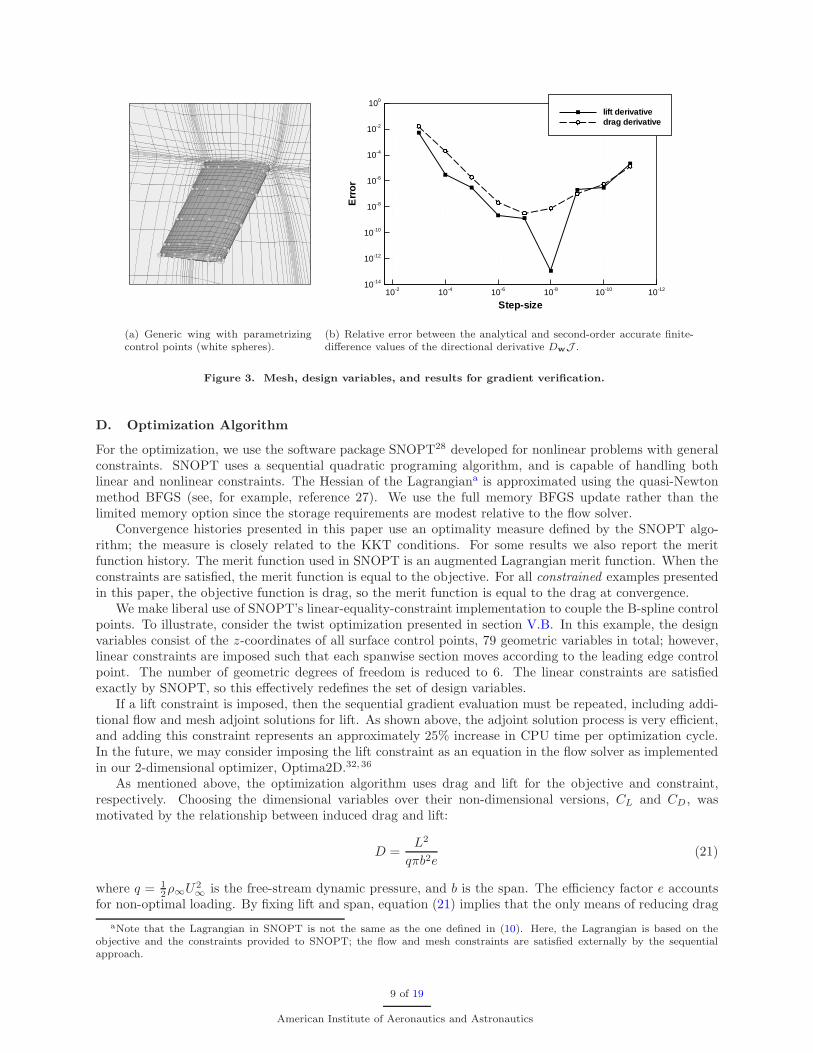
Given the complexity of the algorithm and the use of hand differentiation, verifying gradient accuracy isimportant. Consider a 12 block mesh around a generic wing with no sweep; see Figure 3(a). Each blockconsists of 23× 33× 17 nodes and is fit with B-spline volumes. The wing is parametrized using the B-splinecontrol points corresponding to the surface; these control points are depicted as white markers in Figure3(a). In total, there are 297 geometric design variables. This total excludes the y-coordinate of control pointson the symmetry plane and all coordinates of one control point on the symmetry plane, which is fixed toprevent translation.

Including the angle of attack, there are 298 design variables. Checking each computed gradient componentagainst a finite-difference approximation would be time consuming and unnecessary. We use a directionalderivative to check all the gradient components simultaneously. For a given direction w the analyticaldirectional derivative is given by

DwJ =∂J

∂vw

while the second-order finite-difference approximation is

J (v + ǫw) − J (v − ǫw)

2ǫ= DwJ + O(ǫ2)

where ǫ is the perturbation parameter.Individual components of the gradient can differ in magnitude by 2–4 orders. It is tempting, therefore, to

choose a direction w such that each element of the gradient makes an equal contribution to DwJ ; however,this tends to increase the step-size range over which round-off errors affect the finite-difference approximation.Instead, we use the direction

(w)i = sign

[(

∂J

∂v

)

i

]

,

which gives a directional derivative equal to the L1 norm of the gradient. This direction may help reducesubtractive cancellation between gradient components.

Figure 3(b) plots the relative error between the analytical and finite-difference values of DwJ , where theobjective is either lift or drag. For each objective, the free-stream Mach number was fixed at 0.5 and theangle of attack at four degrees. The plot shows the expected second-order convergence of the finite-differenceapproximation, and its eventual contamination by round-off errors. These results suggest that the analyticalgradients are at least as accurate as their finite-difference approximations with optimal step sizes.

8 of 19


(a) Generic wing with parametrizingcontrol points (white spheres).

Step-size

Erro

r

10-1210-1010-810-610-410-210-14

10-12

10-10

10-8

10-6

10-4

10-2

100

lift derivativedrag derivative

(b) Relative error between the analytical and second-order accurate finite-difference values of the directional derivative DwJ .

Figure 3. Mesh, design variables, and results for gradient verification.

D. Optimization Algorithm

For the optimization, we use the software package SNOPT28 developed for nonlinear problems with generalconstraints. SNOPT uses a sequential quadratic programing algorithm, and is capable of handling bothlinear and nonlinear constraints. The Hessian of the Lagrangiana is approximated using the quasi-Newtonmethod BFGS (see, for example, reference 27). We use the full memory BFGS update rather than thelimited memory option since the storage requirements are modest relative to the flow solver.

Convergence histories presented in this paper use an optimality measure defined by the SNOPT algo-rithm; the measure is closely related to the KKT conditions. For some results we also report the meritfunction history. The merit function used in SNOPT is an augmented Lagrangian merit function. When theconstraints are satisfied, the merit function is equal to the objective. For all constrained examples presentedin this paper, the objective function is drag, so the merit function is equal to the drag at convergence.

We make liberal use of SNOPT’s linear-equality-constraint implementation to couple the B-spline controlpoints. To illustrate, consider the twist optimization presented in section V.B. In this example, the designvariables consist of the z-coordinates of all surface control points, 79 geometric variables in total; however,linear constraints are imposed such that each spanwise section moves according to the leading edge controlpoint. The number of geometric degrees of freedom is reduced to 6. The linear constraints are satisfiedexactly by SNOPT, so this effectively redefines the set of design variables.

If a lift constraint is imposed, then the sequential gradient evaluation must be repeated, including addi-tional flow and mesh adjoint solutions for lift. As shown above, the adjoint solution process is very efficient,and adding this constraint represents an approximately 25% increase in CPU time per optimization cycle.In the future, we may consider imposing the lift constraint as an equation in the flow solver as implementedin our 2-dimensional optimizer, Optima2D.32, 36

As mentioned above, the optimization algorithm uses drag and lift for the objective and constraint,respectively. Choosing the dimensional variables over their non-dimensional versions, CL and CD, wasmotivated by the relationship between induced drag and lift:

D =L2

qπb2e(21)

where q = 12ρ∞U2

∞ is the free-stream dynamic pressure, and b is the span. The efficiency factor e accountsfor non-optimal loading. By fixing lift and span, equation (21) implies that the only means of reducing drag

aNote that the Lagrangian in SNOPT is not the same as the one defined in (10). Here, the Lagrangian is based on theobjective and the constraints provided to SNOPT; the flow and mesh constraints are satisfied externally by the sequentialapproach.

9 of 19


Function evaluations0 5 10 15 20 25 30

10-30

10-25

10-20

10-15

10-10

10-5

100

objective function

optimality

Figure 4. Convergence history for the inverse

design verification.

Function evaluations0 5 10 15 20 25

10-12

10-10

10-8

10-6

10-4

10-2

optimality

constraint violation

Figure 5. Convergence history for the twist

optimization case.

is through the efficiency factor.

V. Verification and Validation

In this section, we verify and validate the optimizer using inverse design and twist optimization. Inversedesign is a common verification for aerodynamic optimization. The intention with twist optimization is torecover the elliptical lift distribution predicted by linear theory. To our knowledge, twist optimization hasnot been used as a validation case in the literature.

The lift, drag, and area values reported in this section and the next are based on the half-span geometry.Unless otherwise indicated, the reference area is the projected area of the initial shape. In all examplesthe reference area is fixed, so we can report coefficients of lift and drag, rather than lift and drag, withoutambiguity.

A. Inverse Design

As a simple verification, we consider an inverse design based on surface pressure. The design variablesconsist of the angle of attack and the 3 coordinates of a control point on the upper surface of the wingshown in Figure 3(a). The initial angle of attack is four degrees. The target design is produced by randomlyperturbing the 4 design variables. The optimizer is given the unperturbed wing and angle of attack as theinitial design; the goal is to recover the perturbed shape and angle of attack based on a target pressuredistribution.

To obtain the target pressure distribution, we solve for the flow around the perturbed wing and angle ofattack at a Mach number of 0.5. For the inverse design problem, the objective is defined by

J =1

2

Nsurf∑

i=1

(pi − pi,targ)2∆Ai

where Nsurf is the total number of surface nodes, and ∆Ai is the surface area element at node i. The pressureand target pressure at node i are denoted by pi and pi,targ respectively.

Figure 4 shows the convergence history for the inverse design problem. The gradient converges 10 ordersand the objective converges 20 orders in 25 objective function and gradient evaluations.

B. Twist Optimization

According to linear aerodynamic theory, induced drag for a planar wake is minimized by an elliptical span-wise lift distribution; thus, linear theory provides a useful benchmark for optimization algorithms. This

10 of 19


X

Z

Y

(a) Initial untwisted wing

X

Z

Y

(b) Optimized twist

y

Lift(

y)

0 0.5 1 1.5 20

0.05

0.1

0.15

0.2

0.25

0.3

0.35

untwisted distributionelliptical distribution

(c) Initial distribution

yLi

ft(y)

0 0.5 1 1.5 20

0.05

0.1

0.15

0.2

0.25

0.3

0.35

optimized distributionelliptical distribution

(d) Optimized distribution

Figure 6. Initial and optimized designs and their lift distributions.

is also a challenging benchmark: the analysis in Appendix A shows that a perturbation of order ǫ in thelift distribution produces an order ǫ2 perturbation in the induced drag. Hence, obtaining an optimal liftdistribution close to elliptical requires sufficient accuracy in the drag prediction.

As is well known, elliptic lift distributions are not unique. The same distribution can be obtained usingchanges in planform, twist, sectional lift, or some combination of these. For this validation, we vary thetwist. The design examples, presented below, will illustrate why planform is a poor choice for recovering theoptimal distribution predicted by linear theory.

The initial geometry consists of a rectangular wing with NACA 0012 sections, a chord length of 2/3 anda semi-span of 2. The reference area is 4/3. The grid has a 12 block topology with approximately 1.158×106

nodes. The blocks are fit with B-spline volumes such that the wing surface is parametrized with 9×7 controlpoints on the upper and lower patches; the parametrization is similar to the one in Figure 3(a). The Machnumber is 0.5 and the angle of attack is fixed at 4.2416◦ to avoid non-unique designs. This particular angleof attack ensures that the initial design meets the CL constraint of 0.375.

The trailing edge control points are fixed, and linear constraints are applied such that the twist of eachspanwise station is a function of the z-coordinate of the leading edge control point. Fixing the trailing edgehelps reduce non-planar effects, although, side-edge separation37 makes a completely planar wake difficultto achieve in practice. Finally, the twist of the wingtip edge is constrained to be the same as the twist atthe neighbouring control point section; this constraint is necessary to prevent mini-winglets.

The convergence history for the twist optimization is shown in Figure 5. After 21 function evaluationsthe optimality measure has been reduced 4 orders of magnitude and the absolute constraint violation hasbeen reduced below 10−12. The coefficient of drag has been reduced approximately 2.1% from 0.00755 to0.00739. The optimal induced drag predicted by lifting line theory, based on CL = 0.375, is CD,i = 0.00746;numerical errors may be responsible for the slightly lower drag produced by the algorithm.

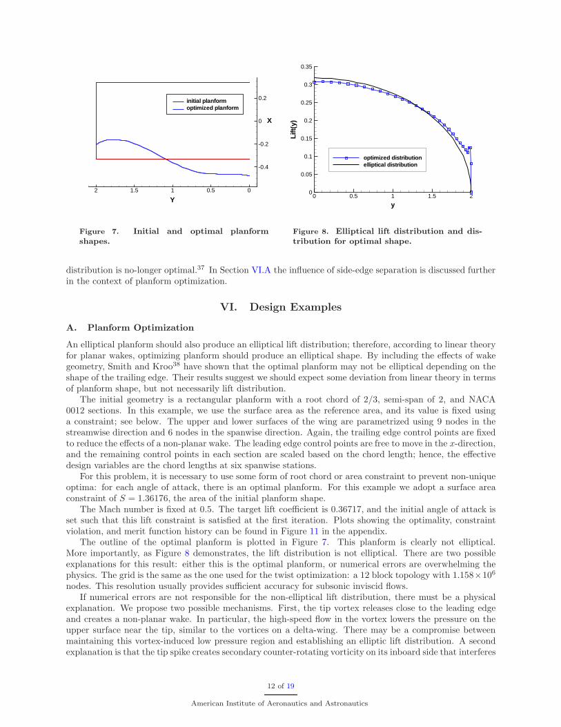
Figure 6 shows the geometry and lift distribution for the initial and optimized designs. In contrast to theinitial shape, the optimized shape exhibits a lift distribution close to elliptical. A small discrepancy betweenthe elliptical and optimized distribution is visible at the wing tip. The increased sectional lift is caused bythe tip vortex. The side-edge separation induces a non-planar wake which implies that the elliptical lift

11 of 19


-0.4

-0.2

0

0.2

Y00.511.52

X

initial planformoptimized planform

Figure 7. Initial and optimal planform

shapes.

y

Lift(

y)

0 0.5 1 1.5 20

0.05

0.1

0.15

0.2

0.25

0.3

0.35

optimized distributionelliptical distribution

Figure 8. Elliptical lift distribution and dis-

tribution for optimal shape.

distribution is no-longer optimal.37 In Section VI.A the influence of side-edge separation is discussed furtherin the context of planform optimization.

VI. Design Examples

A. Planform Optimization

An elliptical planform should also produce an elliptical lift distribution; therefore, according to linear theoryfor planar wakes, optimizing planform should produce an elliptical shape. By including the effects of wakegeometry, Smith and Kroo38 have shown that the optimal planform may not be elliptical depending on theshape of the trailing edge. Their results suggest we should expect some deviation from linear theory in termsof planform shape, but not necessarily lift distribution.

The initial geometry is a rectangular planform with a root chord of 2/3, semi-span of 2, and NACA0012 sections. In this example, we use the surface area as the reference area, and its value is fixed usinga constraint; see below. The upper and lower surfaces of the wing are parametrized using 9 nodes in thestreamwise direction and 6 nodes in the spanwise direction. Again, the trailing edge control points are fixedto reduce the effects of a non-planar wake. The leading edge control points are free to move in the x-direction,and the remaining control points in each section are scaled based on the chord length; hence, the effectivedesign variables are the chord lengths at six spanwise stations.

For this problem, it is necessary to use some form of root chord or area constraint to prevent non-uniqueoptima: for each angle of attack, there is an optimal planform. For this example we adopt a surface areaconstraint of S = 1.36176, the area of the initial planform shape.

The Mach number is fixed at 0.5. The target lift coefficient is 0.36717, and the initial angle of attack isset such that this lift constraint is satisfied at the first iteration. Plots showing the optimality, constraintviolation, and merit function history can be found in Figure 11 in the appendix.

The outline of the optimal planform is plotted in Figure 7. This planform is clearly not elliptical.More importantly, as Figure 8 demonstrates, the lift distribution is not elliptical. There are two possibleexplanations for this result: either this is the optimal planform, or numerical errors are overwhelming thephysics. The grid is the same as the one used for the twist optimization: a 12 block topology with 1.158×106

nodes. This resolution usually provides sufficient accuracy for subsonic inviscid flows.If numerical errors are not responsible for the non-elliptical lift distribution, there must be a physical

explanation. We propose two possible mechanisms. First, the tip vortex releases close to the leading edgeand creates a non-planar wake. In particular, the high-speed flow in the vortex lowers the pressure on theupper surface near the tip, similar to the vortices on a delta-wing. There may be a compromise betweenmaintaining this vortex-induced low pressure region and establishing an elliptic lift distribution. A secondexplanation is that the tip spike creates secondary counter-rotating vorticity on its inboard side that interferes

12 of 19


Y-2 -1.5 -1 -0.5 0 0.5 1 1.5 2

-0.2

0

0.2

Z

(a) Initial flat wing: CD = 0.00752

Y-2 -1.5 -1 -0.5 0 0.5 1 1.5 2

-0.2

0

0.2

Z

(b) Optimized spanwise vertical shape: CD = 0.0069

Y-2 -1.5 -1 -0.5 0 0.5 1 1.5 2

-0.2

0

0.2

Z

(c) Local optimum of spanwise vertical shape: CD = 0.00723

Figure 9. Initial and optimized designs for spanwise vertical shape.

with the primary tip vortex.Whatever mechanism is responsible for the optimal planform, the improvement over an elliptically loaded

wing is small; see Figure 11(b). This is consistent with the analysis in Appendix A. Consequently, induceddrag would likely have a negligible influence in a more realistic planform optimization including viscous andwave drag, and non-aerodynamic disciplines.

B. Spanwise Vertical Shape Optimization: Winglet Generation

For a fixed span, non-planar configurations can produce much lower induced drag than those with planarwakes. In this section and the next we consider examples that exploit non-planar wakes.

Again, the initial geometry is a rectangular wing with NACA 0012 sections, a semi-span of 2, and chordlength of 2/3. The grid is fit using B-spline volumes, with 9×5 control points on the upper and lower surfacesof the wing, in the streamwise and spanwise direction, respectively. The 5 spanwise control point sectionsare free to move in the vertical direction provided no control point exceeds the bounds −0.2 ≤ z ≤ 0.2.Permitting all spanwise stations to move introduces non-uniqueness in the design space, since many designscan be translated within the box constraints; however, the final designs are unique, because the upper andlower bound constraints are active.

The Mach number is fixed at 0.5 and a CL constraint of 0.375 is imposed, based on a reference area of4/3. The initial angle of attack is set to satisfy the lift constraint. Convergence plots of optimality, constraintviolation, and merit function are provided in the appendix, Figure 12.

The initial and optimized designs are shown in Figures 9(a) and 9(b), respectively. The optimized designhas maximized the vertical extent near the tip, which Kroo has remarked is the “critical parameter” for non-planar systems.3 The initial design has an induced drag of CD = 0.00752, while the final design produces

13 of 19


CD = 0.0069, a reduction of approximately 8.2%. Note that further reductions would be possible if twist orplanform changes were permitted to optimally load the configuration.

To identify possible local optima for this problem, we reran the optimization with the control points at thetip of the initial shape positioned at z = −0.2, thus creating a negative dihedral winglet. Indeed, this initialshape did lead to the distinct optimum shown in Figure 9(c); however, this configuration produces a dragreduction of only 3.9% (CD = 0.00723). Eppler,39 using lifting surface theory with induced lift contributions,also concluded that “winglets up are much better than winglets down, whereas classical theories with rigidwake yield exactly the same (drag).” He attributed this difference to the horizontal component of the boundvortex increasing (decreasing) the distance between the tip vortices for the winglet-up (-down) case, thusincreasing (decreasing) the effective span. Another possible mechanism is the vertical distance that thevortex is moved by the free-stream as the vortex is shed from the tip. In the winglet-up case, the free-streamtends to increase the distance between the vortex and the wing. In contrast, the vortex shed from thewinglet-down shape is swept closer to the wing in the vertical direction.

There is some evidence that the optimal winglet dihedral is strongly influenced by viscous effects. Forexample, Gerontakos and Lee40 varied wingtip dihedral in an experimental investigation and found thatthe winglet-down case produced lower induced drag than the corresponding winglet-up case; however, theynoted that there was an order of magnitude discrepancy between the induced drag predicted by lifting-linetheory and the experimental results obtained using the Maskell wake survey method.41

C. Box-Wing Optimization

In this final example we optimize the loading for a box-wing configuration. For closed systems, like thebox-wing, the optimal loading is not unique.3 For this reason, box-wing configurations offer considerabledesign flexibility.

The initial box-wing geometry has a semi-span of 3.065 and chord length of 1. The initial height tospan ratio is 0.1. A 6 block grid surrounds the box-wing geometry with approximately 6.02 × 105 nodes.The surface is parametrized using 9 control points in the streamwise direction and 5 control points in thespanwise and vertical directions. The vertical surfaces are linearly constrained by the upper and lowerhorizontal surfaces. Along the horizontal surfaces, the leading and trailing edge control points are free tomove vertically within the box constraint |z| ≤ 0.315. A translation constraint is imposed by forcing theupper and lower leading edges at the root to have an average z-coordinate of 0.

Based on the above constraints, the effective design variables are the twist and vertical position of the 5spanwise sections along the upper and lower surfaces. Accounting for the translation constraint, this provides19 degrees of freedom; however, the gradient tends to push the sections to their upper and lower bounds, soonly about half of these degrees of freedom are useful in practice.

The lift coefficient constraint is 0.5, based on a reference area of 3; this constraint is satisfied initiallyusing an angle of attack of 4.13486 degrees. The free-stream Mach number is 0.5.

The convergence history for this problem is provided in Figure 13 in the appendix. SNOPT has convergedthe optimality conditions by approximately 3.5 orders over 53 function evaluations. However, the optimizerwas unable to reduce the optimality below the requested tolerance of 10−7, despite decreasing the flow adjointtolerance to 10−9. This convergence difficulty may be related to the non-unique design space producing asingular Hessian.

Figure 10 shows the pressure contours around the final design. The drag coefficient has been reduced7% from 0.0125 to 0.0116. For a planar configuration with the same lift, linear theory predicts an optimaldrag coefficient of 0.0133; hence, relative to a planar system, the optimized box-wing has reduced the dragby 12.6%.

VII. Summary and Conclusions

We have described a gradient-based algorithm for induced drag minimization. Parametrization and meshmovement are integrated using a B-spline volume mesh approach. Flow solutions are obtained using anefficient parallel Newton-Krylov algorithm and SBP-SAT discretization. A Lagrangian formulation is usedto enforce the mesh movement and flow solution at each optimization design cycle. The objective gradient iscalculated using a discrete adjoint approach. We have shown that the Krylov solver GCROT is an efficientand robust alternative to restarted GMRES when solving the flow adjoints. In the present implementation,

14 of 19


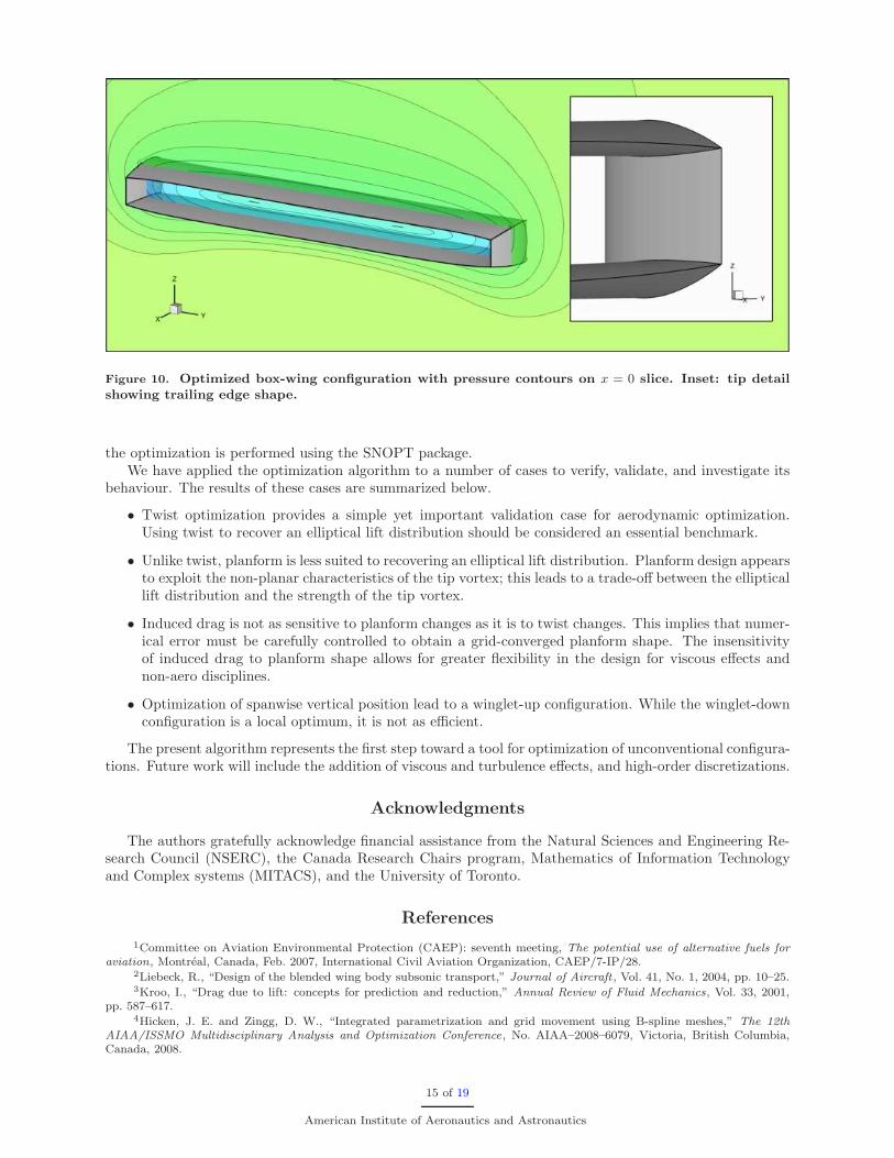
Figure 10. Optimized box-wing configuration with pressure contours on x = 0 slice. Inset: tip detail

showing trailing edge shape.

the optimization is performed using the SNOPT package.We have applied the optimization algorithm to a number of cases to verify, validate, and investigate its

behaviour. The results of these cases are summarized below.

• Twist optimization provides a simple yet important validation case for aerodynamic optimization.Using twist to recover an elliptical lift distribution should be considered an essential benchmark.

• Unlike twist, planform is less suited to recovering an elliptical lift distribution. Planform design appearsto exploit the non-planar characteristics of the tip vortex; this leads to a trade-off between the ellipticallift distribution and the strength of the tip vortex.

• Induced drag is not as sensitive to planform changes as it is to twist changes. This implies that numer-ical error must be carefully controlled to obtain a grid-converged planform shape. The insensitivityof induced drag to planform shape allows for greater flexibility in the design for viscous effects andnon-aero disciplines.

• Optimization of spanwise vertical position lead to a winglet-up configuration. While the winglet-downconfiguration is a local optimum, it is not as efficient.

The present algorithm represents the first step toward a tool for optimization of unconventional configura-tions. Future work will include the addition of viscous and turbulence effects, and high-order discretizations.

Acknowledgments

The authors gratefully acknowledge financial assistance from the Natural Sciences and Engineering Re-search Council (NSERC), the Canada Research Chairs program, Mathematics of Information Technologyand Complex systems (MITACS), and the University of Toronto.

References

1Committee on Aviation Environmental Protection (CAEP): seventh meeting, The potential use of alternative fuels foraviation, Montreal, Canada, Feb. 2007, International Civil Aviation Organization, CAEP/7-IP/28.

2Liebeck, R., “Design of the blended wing body subsonic transport,” Journal of Aircraft , Vol. 41, No. 1, 2004, pp. 10–25.3Kroo, I., “Drag due to lift: concepts for prediction and reduction,” Annual Review of Fluid Mechanics, Vol. 33, 2001,

pp. 587–617.4Hicken, J. E. and Zingg, D. W., “Integrated parametrization and grid movement using B-spline meshes,” The 12th

AIAA/ISSMO Multidisciplinary Analysis and Optimization Conference, No. AIAA–2008–6079, Victoria, British Columbia,Canada, 2008.

15 of 19


5de Boor, C., A practical guide to splines, Springer–Verlag, Berlin, Germany, revised ed., 2001.6Hayes, J. G., Numerical Analysis, chap. Curved knot lines and surfaces with ruled segments, Springer Berlin/ Heidelberg,

1982, pp. 140–156.7Hoschek, J., “Intrinsic parametrization for approximation,” Computer Aided Geometric Design, Vol. 5, No. 1, 1988,

pp. 27–31.8Burgreen, G. W. and Baysal, O., “Three-dimensional aerodynamic shape optimization using discrete sensitivity analysis,”

AIAA Journal , Vol. 34, No. 9, Sept. 1996, pp. 1761–1770.9Nemec, M., Zingg, D. W., and Pulliam, T. H., “Multipoint and multi-objective aerodynamic shape optimization,” AIAA

Journal , Vol. 42, No. 6, 2004, pp. 1057–1065.10Truong, A. H., Oldfield, C. A., and Zingg, D. W., “Mesh movement for a discrete-adjoint Newton-Krylov algorithm for

aerodynamic optimization,” AIAA Journal , Vol. 46, No. 7, July 2008, pp. 1695–1704.11Meijerink, J. A. and van der Vorst, H. A., “An iterative solution method for linear systems of which the coefficient matrix

is a symmetric M-matrix,” Mathematics of Computation, Vol. 31, No. 137, Jan. 1977, pp. 148–162.12Hicken, J. E. and Zingg, D. W., “A parallel Newton-Krylov flow solver for the Euler equations on multi-block grids,”

18th AIAA Computational Fluid Dynamics Conference, No. AIAA–2007–4333, Miami, Florida, United States, June 2007.13Strand, B., “Summation by parts for finite difference approximations for d/dx,” Journal of Computational Physics, , No.

110, 1994, pp. 47–67.14Carpenter, M. H., Gottlieb, D., and Abarbanel, S., “Time-stable boundary conditions for finite-difference schemes solving

hyperbolic systems: methodology and application to high-order compact schemes,” Journal of Computational Physics, , No.111, 1994, pp. 220–236.

15Jameson, A., Schmidt, W., and Turkel, E., “Numerical solution of the Euler equations by finite volume methods usingRunge-Kutta time-stepping schemes,” 14th Fluid and Plasma Dynamics Conference, Palo Alto, CA, 1981, AIAA Paper 81–1259.

16Pulliam, T. H., “Efficient solution methods for the Navier-Stokes equations,” Tech. rep., Lecture Notes for the vonKarman Inst. for Fluid Dynamics Lecture Series: Numerical Techniques for Viscous Flow Computation in TurbomachineryBladings, Brussels, Belgium, Jan. 1986.

17Swanson, R. C. and Turkel, E., “On central-difference and upwind schemes,” Journal of Computational Physics, , No.101, 1992, pp. 292–306.

18Kelley, C. T., Solving Nonlinear Equations With Newton’s Method , Society for Industrial and Applied Mathematics,Philadelphia, PA, 2003.

19Zingg, D. W. and Chisholm, T. T., “Jacobian-free Newton-Krylov methods: issues and solutions,” Proceedings of TheFourth International Conference on Computational Fluid Dynamics, Ghent, Belgium, July 2006.

20Nielsen, E. J., Walters, R. W., Anderson, W. K., and Keyes, D. E., “Application of Newton-Krylov methodology to athree-dimensional unstructured Euler code,” 12th AIAA Computational Fluid Dynamics Conference, San Diego, CA, 1995,AIAA Paper 95–1733.

21Kim, D. B. and Orkwis, P. D., “Jacobian update strategies for quadratic and near-quadratic convergence of Newton andNewton-like implicit schemes,” 31st AIAA Aerospace Sciences Meeting and Exhibit, No. AIAA–93–0878, Reno, Nevada, 1993.

22Saad, Y. and Schultz, M. H., “GMRES: a generalized minimal residual algorithm for solving nonsymmetric linear sys-tems,” SIAM Journal on Scientific and Statistical Computing , Vol. 7, No. 3, July 1986, pp. 856–869.

23Saad, Y., “A flexible inner-outer preconditioned GMRES algorithm,” SIAM Journal on Scientific and Statistical Com-puting , Vol. 14, No. 2, 1993, pp. 461–469.

24Saad, Y., Iterative Methods for Sparse Linear Systems, SIAM, Philadelphia, PA, 2nd ed., 2003.25Gropp, W. D., Kaushik, D. K., Keyes, D. E., and Smith, B. F., “High-performance parallel implicit CFD,” Parallel

Computing , , No. 27, 2001, pp. 337–362.26Saad, Y. and Sosonkina, M., “Distributed Schur complement techniques for general sparse linear systems,” SIAM Journal

of Scientific Computing , Vol. 21, No. 4, 1999, pp. 1337–1357.27Nocedal, J. and Wright, S. J., Numerical Optimization, Springer–Verlag, Berlin, Germany, 1999.28Gill, P. E., Murray, W., and Saunders, M. A., “SNOPT: an SQP algorithm for large-scale constrained optimization,”

SIAM Journal on Optimization, Vol. 12, No. 4, 2002, pp. 979–1006.29Nielsen, E. J. and Kleb, B., “Efficient construction of discrete adjoint operators on unstructured grids by using complex

variables,” The 43rd AIAA Aerospace Sciences Meeting and Exhibit, No. AIAA–2005–0324, Reno, Nevada, 2005.30Squire, W. and Trapp, G., “Using complex variables to estimate derivatives of real functions,” SIAM Review , Vol. 40,

No. 1, 1998, pp. 110–112.31Mader, C. A., Martins, J. R. R. A., and Marta, A. C., “Towards Aircraft Design Using an Automatic Discrete Adjoint

Solver,” 18th AIAA Computational Fluid Dynamics Conference, No. AIAA–2007–3953, Miami, Florida, United States, June2007.

32Nemec, M., Optimal Shape Design of Aerodynamic Configurations: A Newton-Krylov Approach, Ph.D. thesis, Universityof Toronto, 2003.

33de Sturler, E., “Truncation strategies for optimal Krylov subspace methods,” SIAM Journal of Numerical Analysis,Vol. 36, No. 3, 1999, pp. 864–889.

34Griewank, A., Evaluating derivatives, SIAM, Philadelphia, PA, 2000.35Martins, J. R. R. A., personal communication, Feb. 2007.36Zingg, D. W. and Billing, L., “Toward practical aerodynamic design through numerical optimization,” 18th AIAA

Computational Fluid Dynamics Conference, No. AIAA–2007–3950, Miami, Florida, United States, June 2007.37Smith, S. C., “A computational and experimental study of nonlinear aspects of induced drag,” Tech. Rep. NASA TP

3598, National Aeronautics and Space Administration, Ames Research Center, Moffett Field, CA, 94035–1000, 1996.

16 of 19


38Smith, S. C. and Kroo, I. M., “Computation of induced drag for elliptical and crescent-shaped wings,” Journal of Aircraft ,Vol. 30, No. 4, 1993, pp. 446–452.

39Eppler, R., “Induced drag and winglets,” Aerospace Science and Technology , Vol. 1, No. 1, 1997, pp. 3–15.40Gerontakos, P. and Lee, T., “Effects of winglet dihedral on a tip vortex,” Journal of Aircraft , Vol. 43, No. 1, 2006,

pp. 117–124.41Maskell, E., “Progress towards a method for the measurement of the components of the drag of a wing of finite span,”

Tech. Rep. RAE 72232, Royal Aircraft Establishment, 1973.42Anderson, J. D., Fundamentals of aerodynamics, McGraw–Hill, Inc., New York, NY, 3rd ed., 2001.43Vretblad, A., Fourier analysis and its applications, Springer–Verlag, New York, NY, 2003.

A. Effect of Perturbations on the Lift Distribution and Induced Drag

Consider a planar wing with an elliptical lift distribution, defined by its circulation Γ(y), where y is thespanwise coordinate. Using the transformation y = − b

2 cos(θ), where 0 ≤ θ ≤ π and b is the span, theelliptical distribution can be expressed as (see, for example, reference 42)

Γellip(θ) = 2bV A1 sin(θ).

V denotes the free-stream velocity magnitude. The lift coefficient is determined by the coefficient A1;

specifically, CL = A1πb2

S, where S is the reference area.

Next, consider an arbitrary C2 perturbation of the elliptical lift distribution. This smoothness assumptionis reasonable for a subsonic steady flow. Using a Fourier sine series, the perturbed lift distribution can bewritten as

Γ(θ) = 2bV A1 sin(θ) + ǫ

[

2bV∞∑

n=2

An sin(nθ)

]

,

where ǫ controls the magnitude of the perturbation. The elliptical and perturbed distributions produce thesame lift, since the leading coefficient A1 is the same. In addition, it is easy to show that the L2 norm ofthe perturbation is bounded by ǫ:

‖Γ − Γellip‖2 = O(ǫ) (22)

We are interested in the relationship between ǫ and the induced drag of the perturbed lift distribution.For the subsequent analysis, we need the following bound on the coefficients An, which is a consequence ofΓ ∈ C2 and Fourier theory (see, for example, theorem 4.4 from Vretblad43):

|An| ≤c

n2(23)

for some constant c ∈ R. Now, the induced drag for the elliptical lift distribution is simply

CD,i,ellip =πb2A2

1

S,

and for the perturbed distribution we have,42

CD,i =

(

πb2A21

S

)

[

1 + ǫ2∞∑

n=2

n

(

An

A1

)2]

≤

(

πb2A21

S

)

[

1 +

(

ǫc

A1

)2 ∞∑

n=2

1

n3

]

(using inequality (23))

≤

(

πb2A21

S

)

[

1 +

(

ǫc

A1

)2(π2

6− 1

)

]

(sum of bounding p-series, p = 2)

Thus, we have shown that the difference between the induced drags of the perturbed and elliptical distribu-tions has the following asymptotic behaviour:

|CD,i − CD,i,ellip| = O(ǫ2) (24)

On the one hand, equations (22) and (24) suggest that a fairly large perturbation of the elliptical liftdistribution will have a small effect on the induced drag. On the other hand, these equations underscorethe difficulty of recovering the elliptical lift distribution through optimization: if we want to obtain a liftdistribution that is within ǫ of the elliptical distribution, the induced drag must be accurate to within ǫ2.

17 of 19


B. Optimization Convergence Histories

A. Planform Optimization


10-12

10-10

10-8

10-6

10-4

10-2

100


optimality

(a) optimality and constraint violation


0.00714

0.00716

0.00718

0.0072

0.00722

0.00724

0.00726merit function

(b) merit function

Figure 11. Convergence history for the planform shape optimization. Note that the merit function becomesthe objective (drag) as the constraint violation goes to zero.

B. Spanwise Vertical Shape Optimization

Function evaluations0 5 10 15 20

10-12

10-10

10-8

10-6

10-4

10-2

100


optimality


Function evaluations0 5 10 15 20

0.0068

0.0069

0.007

0.0071

0.0072

0.0073

0.0074

0.0075


(b) merit function

Figure 12. Convergence history for the spanwise vertical shape optimization. Note that the merit functionbecomes the objective (drag) as the constraint violation goes to zero.

18 of 19


C. Box-Wing Optimization


10-13

10-11

10-9

10-7

10-5

10-3

10-1


optimality



0.0114

0.0116

0.0118

0.012

0.0122

0.0124


(b) merit function

Figure 13. Convergence history for the box-wing configuration shape optimization. Note that the meritfunction becomes the objective (drag) as the constraint violation goes to zero.

19 of 19


Documents

An investigation of induced drag minimization using a …oddjob.utias.utoronto.ca/dwz/Miscellaneous/HZ_aiaa_opt_MDO_2008.pdf · An investigation of induced drag minimization ... The