Luis Gustavo Trapp* Evaluation of nacelle drag using ... · to obtain four drag components: wave, induced, viscous and spurious drag ... of fundamentals of physics of CFD drag extraction,

J. Aerosp.Technol. Manag., São José dos Campos, Vol.2, No.2, pp. 145-154, May-Aug., 2010 145

Luis Gustavo Trapp*Empresa Brasileira de Aeronáutica S.A.

São José dos Campos – [email protected]

Henrique Gustavo ArgentieriEmpresa Brasileira de Aeronáutica S.A.

São José dos Campos – [email protected]

*author for correspondence

Evaluation of nacelle drag using Computational Fluid Dynamics Abstract: Thrust and drag components must be defined and properly accounted in order to estimate aircraft performance, and this hard task is particularty essential for propulsion system where drag components are functions of engine operating conditions. The present work describes a numerical method used to calculate the drag in different nacelles, long and short ducted. Two- and three-dimensional calculations were performed, solving the Reynolds Averaged Navier-Stokes (RANS) equations with a commercial Computational Fluid Dynamics (CFD) code. It is then possible to obtain four drag components: wave, induced, viscous and spurious drag using a far-field formulation. An expression in terms of entropy variations was shown and drag for different nacelle geometries was estimated.Keywords: CFD, Drag, Engine, Nacelle, Propulsion.

INTRODUCTION

Evaluation of the performance of an aircraft during its development process is done using different tools. One starts with statistical databases during the conceptual phase; proceeds to CFD or analytical tools during preliminary design together with wind tunnel tests, and ends up in the certification phase, with the actual performance measurement on the aircraft.

The ability to accurately predict the aerodynamic drag, more specifically the correct contribution of each drag component, could represent a strategic commercial advantage. For example, the addition of some drag counts could represent passenger limitations in some commercial airplane routes; consequently, the direct operation costs (DOC) increase, making the airplane less attractive for potential customers.

The major aircraft performance parameters are drag and lift, which together with an engine deck can be used to evaluate other major aircraft characteristics: range, climb rate, maximum speed, maximum payload and so forth. When comparing lift and drag estimations using CFD, the lift can be more easily estimated given that it is one order of magnitude greater than drag. Even though some advances were made during the last decade, drag estimation using CFD still lacks behind the accuracy of a wind tunnel, with challenges like the accurate prediction of large separation regions and of laminar to turbulent boundary layer transition.

The knowledge on the physical components of the drag is important for the prediction of scale effects on aircraft drag. The aerodynamic drag of an aircraft flying at

transonic speeds can be separated into viscous (or profile) drag, induced drag and wave drag.

• Viscous drag consists of skin friction and form drag actuating inside the boundary layer due to the viscosity.

• Induced drag is produced by a modification on the pressure distribution due to the trailing vortex system that accompanies the lift generation.

• Wave drag, in transonic and supersonic flight speeds, is related to shock waves that induce changes in the boundary layer and pressure distribution over the body surface.

DRAG BOOKKEEPING

The generally accepted method to obtain the installed nacelle drag is to calculate it by subtracting the clean aircraft drag from the drag of the aircraft with nacelles (Flamm and Wilcox, 1995). However, this technique does not allow the separation of the various drag components that contribute to the total installed nacelle drag, which include: interference drag (from the nacelle on the wing and from the wing on the nacelle) and the external and internal nacelle drag. According to Flamm and Wilcox (1995), another disadvantage of this technique is that the data accuracy is reduced because the strain-gauge balance must be selected to measure the drag of the entire model instead of only the nacelles. A workaround to this problem was developed by Bencze (1977) by mounting the aircraft model on a strain-gauge balance and support mechanism, whereas the nacelles were mounted on an independent balance and model support mechanism. Therefore, it was possible to determine the interference drag components after measuring the aircraft and nacelle drag separately.

Received: 04/04/10 Accepted: 27/04/10

doi: 10.5028/jatm.2010.02026410

Trapp, L.G., Argentieri, H.G.

J. Aerosp.Technol. Manag., São José dos Campos, Vol.2, No.2, pp. 145-154, May-Aug., 2010146

Additionally, this improves the accuracy of the nacelle drag measurements since the strain-gauge balances are sized to measure only the nacelle drag. However, this technique is limited in the sense that the nacelle pylon is not modeled.

The split between internal and external nacelle drag is also important because while the propulsion specialists are busy developing an engine and measuring thrust at static conditions, aerodynamic specialists are busy developing an airframe and measuring drag at wind-on conditions, usually in separate organizations and at different locations (SAE, AIR1703). The engine streamtube usually defines what is treated as drag and what is thrust loss: the flow outside the streamtube produces drag, while what is inside the streamtube produces thrust loss (Fig. 1). Nevertheless, the exact definition of the thrust/drag bookkeeping system depends on the agreement between the engine and airframe manufacturers and on the details of the propulsion system.

illustrated the drag decomposition from CFD due the entropy variations in the flow as well as the identification of a spurious contribution due to numerical dissipation of the flow solver algorithm and a proper definition of the boundary layer and shock region. Brodersen et al. (2004) presented the drag computation with the standard near-field method integrating the surface pressure forces and shear stresses, and also a drag breakdown into its physical components, such as viscous, wave, and induced drag, applying a far-field approach so that all results are compared to experimental data. Tognaccini (2005), using a far-field formulation, proposed a thrust-drag accounting system given a numerical solution of the viscous subsonic or transonic flow around an aircraft configuration in power-on condition.

A very simple and useful explanation to understand the near-field and far-field methods is to consider the aerodynamic drag as a force exerted by the flow field in the opposite direction of the body movement. In the same way, by the law of the action and reaction, the body reacts with a force with the same strength and opposite direction. The drag in the body perspective (near-field) comes from forces due to pressure distributions over the body surface and due to skin friction. Alternatively, the drag force calculated in the flow field perspective (far-field) comes from three natural phenomena: shock waves, vortex sheet and viscosity.

The most common method to predict drag consists of the integration of pressure and shear stress acting on the surface analyzed, so-called near-field technique. In this method, the form drag can be successfully determined only if the pressure distribution along the surface is known with great accuracy. For numerical solutions of RANS equations, the problem is mainly related to the presence of numerical artificial dissipation, which produces a spurious drag, and this one becomes negligible only for highly dense grids. Another problem of this method is that the near-field drag only allows the distinction between pressure and friction drag.

An alternative way to calculate aerodynamic forces through surface integration is to compute the forces around a surface enclosing the body. The advantage of this technique is that the shear stress contribution may be neglected if the control surface is located outside the viscous layer; however, an additional term (momentum flux) must be included in the analysis. In this method, the drag is determined from the momentum integral balance by considering fluxes evaluated on a surface far from the body. Oswatitsch (1956) derived a formula of the entropy drag considering first-order effects, in which the drag is expressed as the flux of a function depending only on entropy variations. However, this technique can bring

Figure 1: Airflow inside and around the nacelle.

Besides wind tunnel tests, another way to evaluate nacelle drag is using empirical methods and analytical correlations (based on wind tunnels tests), like ESDU 81024 “Drag of axis-symmetric cowls at zero incidence for subsonic Mach numbers”. However, one disadvantage of this method is that it is seldom the case in actual design to have an axisymmetric nacelle lofting and flow at null angle of attack.

Another alternative is to perform the drag extraction using Computational Fluid Dynamics (CFD) tools. A lot of research has been developed on this subject and the AIAA CFD Drag Prediction Workshop (DPW) has been an opportunity for worldwide CFD researchers to share information about their drag prediction methods since 2001.

Due to the many advantages of drag extraction with CFD, many authors have written about this subject: Sloof (1986) and van der Vooren and Sloof (1990) contain a review of fundamentals of physics of CFD drag extraction, while van Dam (1999) presents an extended and detailed overview of the state of the art on drag prediction methods. Chao and van Dam (1999 and 2006) presented an airfoil and wing drag prediction and decomposition with a wake integration technique which is very close to the far-field formulation. Paparone and Tognaccini (2002)

Evaluation of nacelle drag using Computational Fluid Dynamics


uncertainties if the region integrated is not defined in a way that the spurious drag is eliminated from the calculation.

Theoretical drag characteristics

The integral of force balance in the free stream direction can be formulated as:

⋅ =+ −uV ( )= +

r tp p i ndSxS S S S Sairc in out lat

−⎡⎣ ⎤⎦∞+ +∫ 0 (1)

where:

p: density;

u: velocity component in freestream direction;

V: velocity vector;

p: pressure;

p∞: freestream pressure;

τ : viscous stress vector in freestream direction;

Sairc: aircraft surface;

Sin: inlet surface;

Sout: outlet surface;

Slat: lateral surface.

Figure 2 shows a sketch of the domain and respective control volume.

The right-hand side integral in Eq. (2) represents the reaction forces of the airplane while the left-hand side stands for the total force exerted by the fluid. In the CFD terminology, when the integration is performed using the left-hand side integral in Eq. (2), the near-field method is employed. Conversely, when the integration of the right-hand side in Eq. (2) is computed, the far-field method is considered.

Far-field formulation

The far-field drag extraction method used is based on the Van der Vooren and Destarac (2004) method, which assumes that viscous and wave drag effects can be considered confined within control volumes and that all entropy changes come from these two phenomena.

The key now is to transform the right-hand side of Eq. (2) into an entropy variation function and in separated drag contributions. This formulation can be borrowed from Tognaccini (2005) reference, resulting in the following equation:

D V f sR

f sR

V dVs s sVfar

ΔΔ Δ= − ∇⋅ + ⎛

⎝⎜

⎞

⎠⎟

⎡

⎣⎢⎢

⎤

⎦⎥⎥

⎧⎨⎪

⎩⎪

⎫⎬⎪

⎭⎪∞ ∫

r 1 2

2

(3)

where:

fMs1 2

1= −⋅ ∞g

(4)

fM

Ms2

2

2 2

1 12

= −+ −( )

⋅∞

∞

gg (5)

Δs: s - s∞ (entropy variation);

R: gas constant;

γ: ratio of specific heats;

M∞: freestream Mach number.

In order to perform analyses on two-dimensional nacelle geometries, the equation from Tognaccini (2005) can be simplified to an axisymmetric reference system by taking into account that dV = r.dr.dq. This leads to:

Δ ΔD V f sR

f sR

V rdrs s sRf

Δ = − ∇⋅ + ⎛

⎝⎜

⎞

⎠⎟

⎡

⎣⎢⎢

⎤

⎦⎥⎥

⎧⎨⎪

⎩⎪

⎫⎬⎪

⎭⎪∞2 1 2

2

p r

aar∫ (6)

Where r is the distance from the engine axis of symmetry.

Figure 2: Integration domain.

Equation (1) can be decomposed into two surface integrals as:

+ −( )⋅ =+ −( )r t r tuV p p i ndS uV p p i ndxS

x

airc

−⎡⎣ ⎤⎦ −⎡⎣ ⎤⎦ ⋅∞ ∞∫ SSS S Sin out lat+ +∫ (2)



Volume selection

A solution to minimize the spurious drag in the far-field technique is to limit the integration volume. The definition of the integration boundaries can be made using the definition of the boundary layer and shock wave regions explained by Paparone and Tognaccini (2002). They propose a boundary layer and wake region sensor that simply relates the laminar and turbulent viscosity, defined as:

Fvl t

l

=+μ μμ

(7)

where:

μl: laminar viscosity;

μt: turbulent or eddy viscosity.

The value of Fv is large in the boundary layer and wake while in the remaining part of the domain it is approximately equal to one. Thus the viscous region is selected by defining it with Fv > (1.1*Fv∞), where Fv∞ is the free stream value of the boundary layer sensor.

The selection of the shock wave region relies on a sensor based on another non-dimensional function:

F V pa pshock = ⋅∇

∇

(8)

where:

a: local sound speed.

This sensor is negative in expansion zones (no shock waves) and positive in compression regions. Cells with negative values of Fshock are excluded from the shock wave region.

By using the Rankine-Hugoniot relations, it is possible to estimate the Mach number downstream of the shock (Fcw), and this value is used as cutoff to define the shock wave region establishing the follow correlation:

F Fshock cw> (9)

CFD ANALYSES

The CFD analyses were performed using CFD++, a commercial CFD code based on finite-volume formulation

that can deal with arbitrary mesh types. The Reynolds-Averaged Navier-Stokes three-dimensional equations were solved for the compressible flow using implicit, second-order interpolation, centroid-based polynomials and pre-conditioned relaxation. The turbulence model employed was the realizable k-e. The domain initial conditions were identical to the far-field boundary conditions, in which a characteristic-based velocity inflow/outflow was set, thereby prescribing aircraft speed, temperature, turbulence intensity and length scale.

The drag extraction formulation was applied to three different cases, typically employed in the development and testing of an aircraft:

1) 2D analysis of an isolated DLR-F6 nacelle;

2) 3D analysis of a long-duct nacelle with different contraction ratios;

3) 3D analysis of a wind tunnel model internal drag.

Two-dimensional DLR-F6 nacelle drag

In order to test the drag assessment procedure, the DLR F6 nacelle (AIAA, 2003) was chosen. This is a wind tunnel model, long-duct nacelle, from the wing-body-pylon-nacelle configuration used on the “AIAA Drag Prediction Workshops”. This nacelle geometry is open to the general public and, therefore, can be used in the future to compare results from different authors. The original nacelle is a through-flow nacelle (TFN) approximately axisymmetric, which can be easily used to perform a two-dimensional analysis. Typical dimensions for the DLR-F6 wind tunnel model nacelle are given on Table 1, together with design parameters.

Table 1: DLR-F6 nacelle dimensions and design parametersDimension (mm)

Length 180Highlight diameter 55.1Inlet throat diameter 49.4Fan diameter 54.8Max diameter 76.2Exhaust diameter 50Diffusion ratio 1.1Contraction ratio 1.24

A hexahedral mesh was built around this nacelle, extending 10 nacelle lengths upstream, 20 lengths downstream and 20 fan diameters in the spanwise direction. Figure 3 shows a detail of the mesh, while Table 2 presents the mesh size.



An analysis of different Mach numbers were made at Reynolds number equal to 3 x 106, which was the same Reynolds number at which the DPW measurements were performed. The reference area is 0.1454 m2.

Figure 4 shows isocontours of entropy for the Mach 0.6 case in the integration domain, which extends from the engine axis up to 1.57 times the nacelle maximum diameter, and from the nacelle leading to trailing edge. The integration diameter has also been varied, but when there are no shock waves over the nacelle, it does not affect the drag results even with diameters as low as 5% greater than the maximum nacelle diameter. In the presence of the shock waves, the drag values were up to 0.6 drag counts lower, when reducing the integration domain.

Figure 3: Detail of the DLR-F6 axisymmetric mesh.

Figure 4: Isocontours of entropy on the integration domain, Mach 0.3 case.

Table 2: Mesh sizeTotal nodes number 48,969Total elements number 49,489

A comparison between the near field and far-field drag methodologies for the DLR-F6 nacelle as a function of Mach number is presented on Fig. 5. The drag coefficient calculated with near field methodology is about one drag count higher than the far-field method for most speeds, while at the Mach number 0.85 both methodologies estimate approximately the same drag. At the low speeds, one of the reasons for the difference is that the nacelle has a finite trailing edge which is not accounted for in the fair field methodology. On the other hand, at Mach number 0.85 there is a shock wave on the nacelle exterior, which is more conservatively accounted for in the far-field methodology. Figure 6: Nacelle contours.

Figure 5: DLR-F6 nacelle drag coefficients as a function of Mach number.

Effect of the inlet contraction ratio on nacelle drag

The drag of an isolated nacelle is influenced by four major parameters: length, maximum diameter, nozzle diameter and contraction ratio. The length is a function of the engine length and the design of the inlet expansion rate and nozzle convergence rate, as well as the exhaust mixing length. The maximum diameter is defined by the engine accessories attached to the casing, which must be enveloped by the nacelle contours. The nozzle diameter is linked to engine performance and is fixed for a given engine. The contraction ratio is the ratio between the area of the inlet throat and the area of the highlight (the area contained inside the line that connects the inlet leading edge). This ratio affects both the cruise and takeoff performances. A small ratio produces a small cruise drag, but leaves the inlet sensitive to separation with high angles of attack and during crosswind operation on the ground.

In order to verify the effect of variations of the inlet contraction ratio on drag, a generic long-duct nacelle was employed and changes were made to its original geometry. Figure 6 shows the nacelle contours.



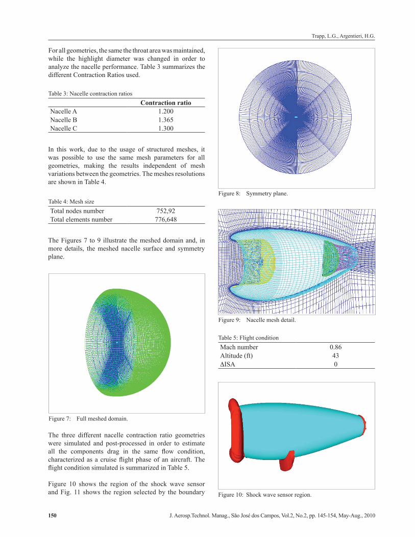
For all geometries, the same the throat area was maintained, while the highlight diameter was changed in order to analyze the nacelle performance. Table 3 summarizes the different Contraction Ratios used.

Table 4: Mesh sizeTotal nodes number 752,92Total elements number 776,648

Table 5: Flight conditionMach number 0.86Altitude (ft) 43∆ISA 0

Figure 7: Full meshed domain.

Figure 8: Symmetry plane.

Figure 9: Nacelle mesh detail.

Figure 10: Shock wave sensor region.

Table 3: Nacelle contraction ratiosContraction ratio

Nacelle A 1.200Nacelle B 1.365Nacelle C 1.300

In this work, due to the usage of structured meshes, it was possible to use the same mesh parameters for all geometries, making the results independent of mesh variations between the geometries. The meshes resolutions are shown in Table 4.

The Figures 7 to 9 illustrate the meshed domain and, in more details, the meshed nacelle surface and symmetry plane.

The three different nacelle contraction ratio geometries were simulated and post-processed in order to estimate all the components drag in the same flow condition, characterized as a cruise flight phase of an aircraft. The flight condition simulated is summarized in Table 5.

Figure 10 shows the region of the shock wave sensor and Fig. 11 shows the region selected by the boundary



Figure 11: Boundary layer sensor region.

Figure 13: Sensitive study of the interpolation cylinder radius’ effect on nacelle drag.

Figure 14: Comparative results of drag for the different geometries.

Figure 12: Nacelle and the cylinder integration volume.

layer sensor. It is important to highlight that the volumes selected by both sensors overlap partially, given that part of the shock wave can be immersed in the boundary layer. Thus it is necessary to apply both sensors together to define the volume where the drag will be calculated. Figure 11 shows the external side of the nacelle with shock waves on the inlet lip, the bottom region near the maximum diameter and near the trailing edge. It also shows a cross cut of the nacelle through the symmetry plane. It can be seen that the volume does not include the internal side of the nacelle (inlet and exhaust regions), which was excluded from the domain after applying the boundary layer sensor.

Given that the two-dimensional DLR-F6 nacelle integrated drag was not very much influenced by the integration volume, the drag accounting procedure was simplified and it was decided to use a cylindrical volume around the nacelle, shown on Fig. 12 in the drag computations, instead of the regions defined by the shock wave and boundary layer sensors,.

A sensitivity analysis of the drag as a function of the cylinder radius was performed and the Fig. 13 shows a sensitive study with different cylinders radii and the respective drag estimation.It can be observed that there is a small increase in drag with the increase in the integration cylinder radius. Nevertheless, the differences between drag values increase by less than 1% though the integrated volume doubles from one case to the next.

According to the flight conditions indicated in Table 5 and by using Eq. (3) with a cylindrical volume of radius equal to 1 m, the results are comparatively summarized in Fig. 14, where Nacelle “B” is the comparison basis (i.e. 100%).

It is noted from Fig. 14 that the best drag performance of Nacelle “A” defines the geometry with the lowest drag and consequently contributes to the best aircraft performance. Further comparisons were made with the ESDU results and revealed that drag values agree within 10%.



Figure 16: Entropy isocontours on the symmetry plane of the integration volume.

Figure 17: Internal nacelle model drag coefficient as a function of Mach number.

Internal drag

As seen before, in turbofan engines, the nacelle drag is assumed to be that one produced outside the stream-tube passing through the intake, therefore it includes the region from the inlet lip stagnation point to the nacelle trailing edge. The effect of the flow on the internal cowlings, supporting structures as well as the pylon portion scrubbed by the engine jet is regarded as a thrust loss. Additionally, when testing a wind tunnel model, it may present other structures that are not present on a real aircraft or engine test bench. Moreover, in case of short-duct nacelles, parts of the pylon will be washed by the engine stream, thus being necessary its removal from the nacelle drag. Fig. 15 shows a typical short-duct nacelle wind tunnel model.

case, such increment is not caused by shock waves, but by the increased separation at the junction between the bifurcation and the inlet duct.

CONCLUSIONS

A comparison of drag methodologies was performed for a two-dimensional case nacelle. Although a fair agreement on drag was found, some important differences still exist. The far-field methodology does not account for the trailing edge and is greatly affected by shock waves when compared to the near field methodology. It remains to be checked whether these differences would be this great if a three-dimensional analysis were made. Nevertheless, this methodology can be easily employed in optimization processes, in which calculating the absolute value of drag is not as important as reaching the minimum drag.

The far-field drag methodology was applied to the evaluation of nacelle drag, showing good agreement with ESDU results and enabling the calculation of more complex nacelle geometries drag. The use of sensors to split the boundary layer and shock regions from the rest of the domain allows the assessment of wave and form drag separately. However, the sensor definition impacts on the size of the integrated region, which could lead

The use of CFD and the far-field formulation present an easy way to perform the split between the external and internal drags. A CFD analysis of the engine and pylon was performed for different Mach numbers, letting the Reynolds number vary and keeping the same sea level ISA condition. The mesh used was a hybrid tetra-prism with approximately 6 million elements.

The integration volume chosen included only the internal nacelle, i.e. the inlet duct the core-cowl bifurcation and the external part of the core cowl that is inside the nacelle and its internal surface. The pylon was not included as well as the core-cowl downstream of the fan nozzle.

Figure 16 shows a cross cut along the nacelle symmetry plane, with isocontours of constant entropy for the Mach 0.75 case, showing the limits of the integration domain along with the main sources of internal drag.

Results of internal drag for the different Mach number cases are shown in Fig. 17 and are consistent with the expected drag levels. When compared to the DLR-F6 nacelle’s two-dimensional results shown previously, there is a drag increase at the highest speeds. In this

Figure 15: Typical short duct nacelle wind tunnel model. Source: Li, Li and Qin, 2000.



to errors on the drag value. It is worth noting, however, that the intensity of the spurious drag is small, as well as its effect on the final result, in both two- and three-dimensional cases.

The separation of internal drag from the overall nacelle (or aircraft) drag was shown to be easily achievable within the post-processing of the results. An identical procedure can be used to analyze the effect of other problems and phenomena on the nacelle, eg.: nacelle inlet lip ice accretion, in case of ice-protection system failure or engine failure; effect of nacelle dents and other protuberances on drag. Even in turboprop engines, a similar method can be employed, evaluating the drag of its intricate shapes, propeller-induced swirl and generally poor aerodynamics of its installations.

It must be remarked that the cases analyzed were subject to completely turbulent flows, without any laminar region and that nowadays many manufacturers are researching nacelles that would allow laminar flow up to 20-30% of the nacelle length. In these cases, an additional validation of this methodology needs to be performed.

REFERENCES

Applied Aerodynamics TC. 2nd AIAA CFD Drag Prediction Workshop, June 21-22, 2003, Available in: http://aaac.larc.nasa.gov/tsab/cfdlarc/aiaa-dpw/Workshop2/workshop2.html Access on May 19, 2010.

Bencze, D.P., 1977, “Experimental Evaluation of Nacelle-Airframe Interference Forces and Pressures at Mach Numbers of 0.9 to 1.4”, NASA Technical Memorandum X-3321, March 1977, Ames Research Center, United States.

Brodersen, O. et al., 2004, “Airbus, ONERA, and DLR Results from the 2nd AIAA Drag PredictionWorkshop”, AIAA Paper No 2004-391, 42nd AIAA Aerospace Sciences Meeting and Exhibit, Reno, Nevada.

Chao, D. D., van Dam, C. P., 1999, “Airfoil Drag Prediction and Decomposition”, Journal of Aircraft, Vol. 36, No. 4, pp. 675-681.

Chao, D. D., van Dam, C. P., 2006, “Wing Drag Prediction and Decomposition”, Journal of Aircraft, Vol. 43, No. 1, pp. 82-90.

ESDU, 2004, “Drag of Axisymmetry Cowls at Zero Incidence for Subsonic Mach Numbers”, Item No. 81024, Engineering Sciences Data Unit.

Flamm. J. D., Wilcox Jr., F. J., 1995, “Drag Measurements of an Axisymmetric Nacelle Mounted on a Flat Plate at Supersonic Speeds”, NASA Technical Memorandum 4660, June 1995, Langley Research Center, United States.

Li, J., Li, F., Qin E., 2000, “Numerical Simulation of Transonic Flow over Wing-Mounted Twin-Engine Transport Aircraft”, Journal of Aircraft, Vol. 37, No. 3, May-June 2000.

Oswatitsch, K., 1956, “Gas Dynamics”, Academic Press Inc, New York, pp. 177-210.

Paparone, L., Tognaccini, R., 2002, “A Method for Drag Decomposition from CFD Calculations”, ICAS 2002 Congress, pp 1113.1-1113.9.

Sloof, J. W., 1986, “Computational Drag Analysis and Minimization; Mission Impossible?”, Proceedings of the Aircraft Drag Prediction and Minimization Symposium, AGARD R-723, Addendum 1.

Tognaccini, R., 2005, “Drag Computation and Breakdown in Power-on Conditions”, Journal of Aircraft, Vol. 42, No. 1, pp. 245-252.

van Dam, C. P., 1999, “Recent Experience with Different Methods of Drag Prediction”, Progress in Aerospace Sciences, Vol. 35, pp. 751-798.

van der Vooren, J., Destarac, D., 2004, “Drag/Thrust Analysis of Jet-Propelled Transonic Transport Aircraft”, Definition of Physical Drag Components, Aerospace Science and Techonolgy, Vol. 8, pp. 545-556.

van der Vooren, J., Sloof, J. W., 1990, “CFD-Based Drag Prediction; State of the Art, Theory”, Prospects, Lectures notes prepared for the AIAA Professional Studies Series, Course on Drag-Prediction and Measurement, Portland (OR).

Documents

Luis Gustavo Trapp* Evaluation of nacelle drag using ... · to obtain four drag components: wave, induced, viscous and spurious drag ... of fundamentals of physics of CFD drag extraction,