239

AN INTRODUCTION TO UNDERWRITING PROFIT MODELS

HOWARD C. MAHLER

Abstract

This paper will provide an introduction to the subject of underwriting profit models in order to provide actuaries with a basic framework for further study. This paper starts with the premise that the subject of underwriting profit provisions is an area in which actuaries can be of assistance in advancing knowledge and developing methods. While this paper will concentrate on the theoretical aspects, this subject has many potential practical applications.

The basic structure of the paper is to start off with an extremely simple model, and then add additional considerations. For clarity, this paper has focused on one basic method of calculating a provision for underwriting profits.

There are three basic ingredients used in these models. First, via a “cashflow” analysis, one estimates the length of time an insurer will have premium dollars on hand, prior to paying losses and expenses. Second, one estimates how much investment income an insurer will earn on this cashflow and the necessary equity backing up the policies. Finally, one sets the expected return on equity equal to a target return on equity. One can then solve this equation for the underwriting profit provision.

INTRODUCTION

The question of what provision for underwriting profits (or losses) to use has become a topic of increasing discussion over the last decade. Rather than use traditional numbers found in the actuarial literature, such as 5%, there have been attempts made to calculate profit provisions. These calculations have involved making certain assumptions and algebraic derivations. Thus they are commonly called underwriting profit “models.” This paper will provide an introduction to the subject, in order to give actuaries a basic framework for further study.

240 I~NI)1-KwHIIIY(r I’KO, I I \101)1.1.2

In spite of the use in the title of the term underwriting profit, this paper concentrates on the total return on equity concept. In each particular case, one can calculate an underwriting margin (positive or negative) that can be expected to produce the desired or required total return on equity. From this point of view there is no fundamental difference between a positive and negative under- writing margin. Equivalently, there is no fundamental difference between a target combined ratio which is greater than 100% and one that is less than 100%. Rather, they are different points along the same continuum.

The basic structure of the paper will be to start off with an extremely simple model, and then add additional considerations. (Those readers already familiar with the subject may want to go directly to the third model or even the summary of that model.) Care has been taken to list all the assumptions made in each model. If, in a particular application, one or more of the assumptions are not reasonable, one can then make the appropriate change in the list of assumptions and derive modified equations. As with most actuarial calculations, the results produced by the models are dependent on the assumptions made and input values used. In actual applications, choosing the appropriate input values is usually a difficult task. (Examples of this are given in the numerical examples using model three and in Appendix II.)

For the reader’s convenience, Appendix I contains the definitions of the various symbols used in this paper.

DEFINITION OF AN UNDERWRITING PROFIT PROVISION

Let P* be the premiums loaded for profits. (The asterisk indicates that P has been loaded for profit. The author has found that this use of the asterisk to denote quantities that are loaded for profit avoids much confusion when working with underwriting profit models.)

In general, ignoring uncollected premium, the underwriting profit provision, u, is defined so that:

P* = P*u + losses + expenses.

This is the fundamental definition of an underwriting profit provision which will be used throughout this paper.

Let f. be the losses paid by the insurer.

The expenses are made up of T*, those expenses which are proportional to

UNDE:RWRITING PROFI7 MODI-.I.S 241

the premium, and E, the remaining expenses. We define F/P* = t. (The use of the letter T comes from premium taxes, which vary with premiums.)

Thus:

P* (l-u) = f. + E + T* = f. + E + rP*

u = 1 - (t + (L+E)IP*)

In this paper we will usually solve for P *, the premium loaded for profits, and then use the above equation to get the underwriting provision u.

THE FIRST MODEL

We make the following assumptions:

(0) An insurer writes a set of similar policies. Each policy is expected to be in effect for one year. (This assumption is labeled zero, since it is so basic that it is often left unstated.)

(I) The insurer receives premiums P*. All premiums are received exactly at policy inception.

(2) The insurer pays losses L. All losses are paid exactly one year after policy inception.

(3) The insurer earns income on its investments at a rate r.

(4) The insurer wishes to break even. (We ignore any investment income the insurer may earn on its equity.)

For this very simple model, we have ignored expenses, equity, income taxes, and all the other complications that exist in the real world. Also, we have assumed that the insurer merely wishes to break even on average. (Under certain circumstances this might be true of a non-profit organization, such as Blue Cross or a Medical Malpractice Joint Underwriting Association.)

We will calculate the premium, P *, the insurer should charge, so that it can be expected to break even. (Elsewhere in the paper, the insurer will desire a return on its equity.) Assumptions (1) and (2) imply that the insurer can invest a sum P* for one year, During that time, rP* investment income will be earned, due to assumption number (3). So the insurer will have P* + rP* available at the end of the policy year. It will have to pay out L at that time, due to assumption (2). Assumption (4) is that the insurer wishes to break even. There- fore:

0 = P* + P*r - L

P* = Li( I +r)

In our special case, t = E = 0. Thus:

u = 1 - LIP* = I - (ISr) = --I

So even this very simple example demonstrates a basic feature. One can have a negative provision for underwriting “profit”. This will occur when the target return is relatively small and/or when you can earn a large amount of investment income (either due to a high rate of return r, or due to a long period of time between when the premiums are received and losses are paid out.) In that case, you can achieve the desired total return, even though you have an underwriting loss. This basic feature has been noted by others, among them Ferrari [l].

THE SECOND MODEL

Until now, we have dealt with a very simple timing of transactions. The value of receiving one dollar depends on when one expects to receive it. See, for example, Kellison [2]. The further in the future one receives it, the less the dollar is worth to you now. In general, we wish to take the present value of the income received. (In taking present values in this paper, we will for convenience always discount to the end of the policy year. Why this is a convenient choice is explained below. In present value equations using a single discount rate, the choice of the point in time to which one discounts should not affect the answer, provided that all terms in the equation are discounted to the same point in time.)

If a dollar is to be received rz years hence, and we discount to the end of the first year, using an interest rate i, then the present value is (I +i)” ~‘I’.

We modify the assumptions of the first model, ( 1) and (2), in order to allow a general timing of the payment of premiums and losses.

(I ‘) The insurer receives premiums P*. (The expected pattern of the timing of payments is known or can be estimated.)

(2’) The insurer pays losses f.. (The expected pattern of the timing of payments is known or can be estimated.)

We modify or add the following assumptions:

(4)The insurer desires a target rate of return of R on the funds it supplies.

UNDtsRWRl-rlNG PROFI1‘ MODl3.S 243

(5a) The insurer supplies funds, S, of its own. These funds exist throughout the entire policy year in a constant amount.

(5b) The required equity S is proportional to the premium P*, with propor- tionality constant s = P*IS.

We have assumed the insurer supplies S at the beginning of the policy year, and desires (1 + R)S back at the end of the policy year.

For the purposes of this paper, these insurer-supplied funds are stockholder- supplied equity. However, the reader may find it helpful to think of them as surplus. These funds in some sense back up a group of policies so that even in the case of unexpected occurrences the insurer will be able to meet its obligation of paying claims.

We have yet to include expenses in the model. Examples of categories of expenses are loss adjustment expense, commissions, other acquisition expenses, general expenses, and premium taxes. (Investment expenses are presumably taken into account by subtracting them from the investment rate of return.) Generally, these expenses can be divided into three types: those that are fixed, those that vary with premium, and those that vary with losses. In this paper, the method by which the specific assignments were made will not be explored. One example of such an assignment is given in Snader [3].

In this paper we will make a slightly different division. First, we include in L those expenses that are assumed to have the same timing as the loss payments. (Alternatively they may have been included in the data from which we made our estimate of the timing of the loss payments.) Next, we separate out those expenses that vary with premiums, and call them T*. (This almost always includes premium taxes, usually includes commissions, and sometimes includes all or part of other acquisition or general expenses.) Whatever expenses are left are called E. (See Appendix II for an example of such assignments. Although the calculations are not shown there, the expense-to-loss ratios depend on a determination of the relative amount of each type of expense. This depends in turn on a determination of which expenses are fixed, and which vary with losses. )

In order to include expenses, we make a minor revision to one of the prior five assumptions; otherwise, we retain them.

(2”) The insurer pays L, losses including those expenses whose timing is the same as the losses. (The expected pattern of the timing of such payments is known or can be estimated.)

244 L’h,)tRWRI 1 IhG PROI 1 I hI0l)l.I S

We also add two additional assumptions

(6) The insurer pays T*. expenses that vary with premiums. (The expected pattern of the timing of such payments is known or can be estimated.)

(7) The insurer pays expenses E, other than those included in f. and r*. (The expected pattern of the timing of such payments is known or can be estimated.)

The insurer earns income from two sources. First. it earns r.S investment income on the equity. Second, it earns income on the cashtlow (premiums in, losses and expenses out.) The present value of the total income earned on the cashflow is P*’ - (L’+E’+T*‘). (The primes denote discounting by the rate of return on investments r.) This is a special case of a more general result. The present value of the total income on a cashflow is the present value of the intlows minus the present values of the outtlows.

For this second model we have

present value of return on equity = (present value of income earned on equity) + (present value of income earned on cashflow)

Setting the target return on equity equal to the present value of the return on equity, we get

RS = rS + P*’ - (L’+E’+T*‘)

Note that RS and r.9 are assumed to be received at the end of the policy year, and thus they are already equal to their present values, since we are discounting to the end of the policy year. (If one had discounted to some other point in time, then this convenient relationship would no longer hold. This is why this point in time was chosen for use in these models.)

Let g = P*‘IP* = P’IP

h = T*‘/T* = T’IT

It should be noted that g and h depend only on the timing of the premium flow and the premium tax flow, and not on their overall magnitudes. Thus they can each be computed from quantities assuming a prolit loading of zero for convenience. This is why we introduce R, h and other similar ratios into the model equations.

245

Then we have

RS = rS + P*’ - (L’ + E’ + T*‘)

P* = (L’ + E’)/(r/s + g - th - R/s)

We use the definition of the underwriting provision, u, when there are expenses

u = I- t - (E+L)/P* = 1 - t - (r/s + g -rh - RIs)I((L’+E’)I(L+E))

Two points are worth making. First, we have not carefully distinguished here between surplus and equity. R is meant to represent the target return on equity, i.e., stockholder-supplied funds. Statutory surplus as defined in the Annual Statement is numerically different from the concept of equity used here, which can be thought of as net worth in accordance with Generally Accepted Accounting Principles (GAAP). It is important that the target return on equity R and the concept of equity S match each other. Adjustments might be appro- priate for certain applications of the model. Among areas where adjustments might be appropriate are the treatment of prepaid expenses and the equity in the unearned premium reserves, estimated federal income taxes and policyholder dividends. The details would depend on the source of and the exact meaning attached to R and S. Unfortunately, the details are beyond the scope of this paper. See, for example, Section 1 of Appendix I to the Report of the Advisory Committee to the NAIC Task Force on Profitability and Investment Income [4], Measurement of Profitability and Treatment of Investment Income in Property Liability Insurance, pp. 783-799 [.5], and Report of the NAIC Investment Income Task Force, p. 43 [6).

Also, the reader should notice that we have not distinguished between the rate of return on investments earned on equity and that assigned to the cashflows. Such a distinction may be appropriate in certain circumstances. For example, you may allocate different types of investments, different maturities of invest- ments, etc., to the equity. Also some of the equity may be in fixed assets which can not be invested. These and other refinements could be reflected in the model.

This model reduces to the previous model if we take the special case where E=T*=O, L’=L, P’=(l+r)P, and either R=r or S=O.

FEDERAL INCOME TAXES

For the moment, let us assume that the insurer will pay income taxes at a rate FIT, one rate for all types of income. Also for the moment, let us ignore the question of the timing of the payment of these income taxes. Then simpl- istically our former equations would be changed, by multiplying all the income terms by (I -FIT). The target rate of return. R. is the desired rate of return after the insurer pays Federal Income Taxes.

RS = (1 -F/T)(rS + P*’ - L’ - E’ - T*‘)

P* = (L’ + E’)( 1 -F/Ty((ris + g - th)( I -F/T) - R/s)

There is no inherent reason to divide the income into different types. How- ever, different types of income are treated differently by the federal income tax system, as is explained in Beckman 171. Income generally is divided into two types, underwriting income (or loss) and investment income. We will assume that the former is taxed at a rate FITCI. In the case of an underwriting loss rather than a profit, FITU should be the rate at which the income that is offset by the underwriting loss would have been taxed. (One can usually assume, for modelling purposes, that the insurer will offset that income which is taxed at the maximum rate first. before using any remainder to offset income taxed at a lower rate. )

We will assume that the investment income is taxed at a rate FITI. (In many implementations, F/T1 will be some sort of weighted average of the tax rate on the different types of investment income. In a later section, an example of such a calculation is given.)

MODEI. THKEE

We make the following assumptions in addition to those in model two.

(8a) Underwriting income is taxed at a rate F/TU. Underwriting income equals premiums minus losses and expenses = P* ~ L ~ E - T*.

@a) Investment income is taxed at a rate FIT/. Investment income is defned as the total income minus underwriting income.

The following assumptions concerning the timing of the payment of taxes have been found useful.

(8b) Federal income taxes on underwriting are paid at the end of the quarter

UNDtRWRlTING PROt~l~I hlODt1.S 247

in which the underwriting profit or loss is incurred.’ (Ignoring any development of incurred losses, this leads to four equal payments at times l/4, 2/4, G and 1 year after policy inception.)

(9b) Federal taxes on investment income on the cashflow are paid at the time losses and expenses are paid.

It is common to make the following assumption, when one has made assumption (5) concerning the equity.

(SC) The Federal income taxes on the investment income earned on the equity are paid at the end of the policy year.

e= present value of federal income taxes on underwriting

federal income taxes on underwriting

The ratio e is dependent only on the timing of the payment of the federal income taxes on underwriting.

Assumption (8b) leads’ to

e = ((1+r)“4 + (1+r)2’4 + (l+r)“4 + (l+r)“)/4

Thus, e is approximately (1 tr)“‘.

Define a ratio d, similar to the previously defined e. Let d = (present value of FIT1 on cashflows)l(FITI on cashflows).

The present value of the total return after taxes can be broken up into five pieces. We have, where PV stands for present value,

PV(tota1 return after taxes) = PV(investment income on equity) - PV(taxes on investment income on equity) + PV(total income on the cashflows) - PV(taxes on underwriting incomej - PV(taxes on investment income on the cashflow)

’ The timing of tax payments does not actually conform to this simplifying assumption. Expenses are deducted from income in accordance with Statutory Accounting Principles (SAP). This advances the recognition of expenses to an earlier time and makes the resulting tax credit more valuable than indicated by assumption (8b). On the other hand, incurred losses (including IBNR) generally develop upwards for long-tailed lines of insurance. This postpones the recognition of losses to a later time and generally makes the tax credit less valuable than indicated by assumption (8b).

’ In a particular application, calculation of a more exact value of e may be appropriate.

We now need to write down expressions for each of these five pieces

PV(investment income on equity) = t-S

Due to assumptions (9a) and (SC),

PV(tax on investment income on equity) = rSFfTl

Also, we have the general result that

PV(tota1 income on the cashflows) = P*’ - L’ ~ E’ - T*’

By definition,

tax on underwriting income = (P” - L ~ E - T*)F/TU

By the definition of c we have

PV(tax on underwriting income) = (P* - I, - E - T*) FlTUe

We have four out of the five pieces we need. In order to get the fifth piece, first we will derive an expression for the investment income on the cashflow. From this will follow the taxes paid on this income and then the present value of these taxes. Unfortunately. this first step will bc a little complicated. We know that

investment income on cashflow = (total income on cashflow) - (underwriting income on cashflow).

We know that the present value of the total income on the cashRows is P*’ - (L’ + E’ + T*‘). In Appendix 111 it is demonstrated, given some not unreasonable assumptions. that we can remove the present value by dividing by a factor F, where .v = (L’ + E’ + T*‘)I(L + E + T*). (Lt is useful to think of this as follows. Multiplying by y would adjust the timing to when the losses and expenses are paid, which is the timing of the total income on the cashflow. Dividing by y backs that timing out.) Therefore

investment income on the cashflows = (P*’ - L’ - E’ - T*‘)& _ (p* - L E ~ T*,

income tax on investment income on the cashflow = FITI((P*’ - L’ - E’ -T*‘)/y ~ (P* ~~ L .~ E -T*))

Then we have from the definition of rf

PV(income tax on investment income on the cashflow) = FITld(( P* ’ - L’ - E’ -T*‘)/? - (I’” L ~ E -T*))

249

Assumption (9b) leads to

d = (L’ + E’ + T*‘)I(L + E + T*) = y

Then we have

PV(income tax on investment income on cashflow) = FITly((P*’ -L’ - E’ -r:‘)/y + (L SE +r: - P*)) = FITl(P*’ - L’ - E’ - T*’ + L’ + E’ + T*’ - P*y) = FITI(P”’ - P*y)

This same result can be arrived at starting with a different approach. See Appendix VI for this approach, using a so-called investment balance for taxes.

Thus, the basic equation becomes

RS = rS -rSFITl +P*‘-L’-El-T*’ -FITUe(P*-L-E-T) - FITI(P*‘-P*y)

We can solve for P*

p* = L’ + E’ - FITUe(L +E) (r/s i- g)( 1 -FITl) - th - R/s + FITiy - (I -t)FITUe

However, y depends in turn on P*, i.e., on the profit loading

y = (L’ + E’ + htP*)i(L + E + tP*)

Fortunately, y is usually relatively insensitive to the profit loading, since it is a weighted average of (L’+E’)/(L+E) and h, wiih weights LIE and tP*.

One can solve numerically via iteration on P* and I’. (For the usual range of input values, the iteration converges very quickly.)

As usual one now uses the defining equation toget the underwriting provision u

u = 1 - (t + (L+E)IP*)

With this third model, we have reached a level of refinement which can be used for real world applications. We will later show how a few more refinements can be added, but of course at the cost of further complexity in the model. (As with any actuarial subject, the question of whether a particular technical reline- ment is worthwhile for a particular application is a matter of judgment. One has to compare the benefits of the extra precision with the extra complications introduced to the model and the cost of obtaining the additional data required.)

SUMMARY OF MODEL THREE

One can solve numerically via iteration on P* and J

p* = L’ + E’ - FITUr(L +E)

(rfs + g)( 1 -FITI) -th - Rls + FITI! - (I -tjF/TUe

y = (L’ + E’ + htP*)l(L + E + tP*)

Then the underwriting provision is given by

u = 1 - (t + (L+E)lP*)

The following assumptions were used

(0) An insurer writes a set of similar policies. Each policy is expected to be in effect for one year.

( 1) The insurer receives premiums P*. (The expected pattern of the timing of payments is known or can be estimated.)

(2) The insurer p”ys losses L, including those expenses whose timing is the same as the losses. (The expected pattern of the timing of such payments is known or can be estimated.)

(3) The insurer earns income on its investments at a rate r.

(4) The insurer desires a target rate of return on equity of R.

(5) The insurer supplies funds, S, of its own. This equity is around through- out the entire policy year in a constant amount. The required equity is propor- tional to the premium, with proportionality constant .s =P*/S.

(6) The insurer pays T*, expenses that vary with premiums. (The expected pattern of the timing of such payments is known or can be estimated.)

(7) The insurer pays expenses E, other than those included in L and T*. (The expected pattern of the timing of such payments is known or can be estimated.)

(8) Underwriting income is taxed at a rate FlTU. Underwriting income equals premiums minus losses and expenses = P* -- L - E - T*. Federal income taxes on underwriting are paid at the end of the quarter in which the underwriting profit or loss is incurred. (Ignoring any development of incurred losses, this leads to four equal payments at times %. ?/J, % and 1 year after policy inception.)

(9) Investment income is taxed at a rate FITI. Investment income is defined as the total income minus underwriting income. Federal income taxes on the investment income earned on the equity, are paid at the end of the policy year. Federal income taxes on investment income earned on the cashflow are paid at the time losses and expenses are paid.

NUMERICAL EXAMPLES USING THE THIRD MODEL

We will use all of the assumptions of this third model, including (8b), (9b), and (SC). We will choose input values which are not unreasonable for a real world insurer. However, these values are for illustrative purposes only. In any application it is very important to choose a consistent set of inputs. If the different input values are chosen independently of each other, one can get unusual results to say the least. Just as in ratemaking, the answer is only as valid as the assumptions of the method and the input values chosen.

For the target rate of return on equity after taxes, R, we will use 17%. This may have been given to the actuary by the president of the insurer, the com- missioner of insurance, etc. It may have been estimated by looking at the rates of return earned by similar firms or industries. It may have been estimated by using an economic model such as the Capital Asset Pricing Model (CAPM), together with the observed “risk free” rate of return available on U.S. Treasury securities of the appropriate maturities. It may have been estimated by looking at the past results for that line of insurance in competitive markets. Of course, another method or combination of methods may have been used.

There are a number of questions of interest concerning the rate of return on equity. Should rates of return be measured with respect to book or market value of equity? Should the target rate of return differ by line of insurance? How does the target rate of return depend on the other inputs, among them the types of investments and the premium-to-equity ratio?

For the premium-to-equity ratio, s, we will use a value of 2. In the model, we are really interested in stockholder equity, rather than statutory surplus. Therefore, as stated previously, if one is trying to estimate s from data, various adjustments may have to be made to switch from the Annual Statement to Generally Accepted Accounting Principles (GAAP). As stated above, an im- portant consideration is whether one should use the book or market value of equity. Another important consideration would be whether to adjust the equity for the effect of the discounting of loss reserves. Another question of interest

is whether different lines of insurance have different acceptable or desirable premium-to-equity ratios.

For the rate of return on investments before taxes, I’. we will use 10%. The rate of return, as well as the tax rate. depend on what types of investment the insurer will hold. Also, an insurer who takes more investment risk will generally expect a higher target rate of return, R. One of the questions of interest is whether to use the “imbedded” yields an insurer can be expected to earn on his current portfolio, or whether to use the current yields one could obtain by investing fresh funds. Generally. the rate of return on investments should be measured after taking into account necessary investment expense.

For the federal income tax rate on investment income, F/T/, we will use 28%. As stated previously, the value of FITI would depend on the proportion of each type of asset held, and the rate of return cxpectcd on each type of asset.

For the federal income tax rate on underwriting income, F/RI, we will use 46%. This is the current maximum corporate rate. In the event of an underwriting loss, the 46% tax rate would only be appropriate if there was sufficient income that would be taxed at the 46% rate, so as to be offset by the underwriting loss. As pointed out in Beckman [7]. interest from tax-exempt bonds is not taxed and long term capital gains are taxed at less than the corporate rate. (While 858 of dividends on stocks can be deducted from net taxable income, the remaining 1.5% is taxable at the full corporate rate.)

We will use a ratio of variable expenses to premium. 1, of 20%.

For simplicity, we will assume here that all the premium is collected at policy inception. and that all the variable expenses are paid out at policy inception. Also, we will assume that fixed expenses and losses are all paid precisely N years after policy inception. (These are unrealistic simplifications, but in Appendix II is a numerical example for private passenger automobile property damage liability. with more realistic timing assumptions.)

Assuming an arbitrary $800 for losses plus fixed expenses, we get

N(years) P*

.5 $1,044 1.0 980 1.5 916 2.0 853

v 2

I.059 1.020 ,981 .943

Underwriting Profit Provisions

3.4% -1.6%~ -7.3%

- 13.8%

UhI~l,RWWl’,‘ING PROF’,, 1,O,,,~.,.S 253

Note: as we shall see later, the profit provision calculated above for N=2 assumes that there is income taxable at 46%, available from other than the investment income on this line of insurance and the equity backing it up, that can be offset by a portion of the projected underwriting loss.

We notice that all other things being equal, the larger N, i.e., the longer tailed the line of insurance, the more negative the profit provision. As has been mentioned above, there is no fundamental difference between positive and negative underwriting margins. We can see here that they are merely different points along the same continuum.

SENSITIVITY TO VARIOUS INPUTS

It is of interest to see how the underwriting profit provision changes as we vary one input at a time. Above we have already seen how the profit provision varies as the length of the cashflow changes. Let’s now hold the length of the cashflow constant at N= I. For the set of inputs used above this gave a profit provision of - 1.6%.

As expected, if you desire a higher target rate of return, you must have a more positive underwriting profit provision, all other things being equal. If you can earn a higher return on investments, you can afford a less positive under- writing profit provision. When you have a higher premium-to-equity ratio, you can afford a less positive profit provision. When you have a projected under- writing loss, the higher the federal income tax rate on underwriting, the more negative the profit provision, since the “tax shield” is worth more. The situation is reversed when you project an underwriting gain. The profit provision gets more sensitive to FITU as the profit provision gets further from zero. Finally, the higher the rate of federal income taxes on investments, the more positive the profit provision. The profit provision gets more sensitive to the value of FITI as the cashflow gets longer, and thus more investment income can be earned.

We have varied the different inputs one at a time. In actual practice, many of the inputs will depend on one another. Thus, one can not just vary them independently of each other. However, it is still enlightening to see how the profit provision varies, all other things being equal.

One could perform a similar analysis using differentiation. This is outlined in Appendix V.

SENSITIVI I’\ ‘I‘0 VARIOUS INPUTS

Assumptions

target return on equity R= 16% R= 17% R=l8%

rate of return on investments r=97+ r= 10% r=Il%

premium-to-equity ratio s= I .5 s=2.0 s=2.5

federal income tax rate on underwriting FITU = 30% FITU=46%

federal income tax rate on investments FITI= 18% FITI=28% FlTl=38%

Underwriting Profit

Provision

-2.6% -1.6% -0.7%’

0.1% - I .6% -3.45%

I .5%’ - 1.6% -3.5%

~ I .2% -- I .6%

-4.1% -1.6%

0.8%

A COMPUTATION OF THE AVERAGE INCOME TAX RATE ON INVESTMENTS

In the previous numerical examples, a 10% rate of return and a 28% tax rate on investment income were used. Here is one possible source for these values.

Make the following specific assumptions as to the source of the projected invested income. Assume that the insurer will have his assets invested solely in bonds, one half taxable, and one half tax-exempt. Further, assume that the taxable bonds will return 12% before taxes, while the tax-exempts will earn 8%. Then the rate of return, r, and the federal income tax rate on investment income, FITI, can be computed as follows.

Type of Asset Amount Rate of Return Income Tax rate Tax ___ -

Taxable Bond .5 12% .06 46% .0276 Tax-Exempt Bond .5 8% .04 0% 0

- - -

Combined 1.0 .I0 .0276

Thus the combined rate of return is IO/l .O = 10%. The combined tax rate is .0276/. IO = 27.6%, or 28% to the nearest percent. This matches the choices of r= 10% and FfTI=28%. which were made for the numerical models above.

TAX SHIELD, UNDERWRITING LOSSES

We have seen that underwriting losses can be used to offset otherwise taxable income. As such they have a potential value, which can be only realized if there is taxable income available to be offset. In general, when one has a negative provision for underwriting profits, one should check whether income is available to be offset that would have been taxed at the value of FITU chosen.

Here we will check our numerical examples from above to see whether there is enough income taxed at 46%, so as to be offset by our projected underwriting loss. We will use the distribution of assets and rates of return on assets from the previous section.

How much taxable income is available to be offset by an underwriting loss? From the previous section, .06/. IO = 60% of the pre-tax investment income is taxable (at 46%).

256 , YII,.K\\‘KI,IU<r I’KO, I, ZI0I)L.I \;

We have for model three

investment income on the cashflows = (p*’ - L’ - E’ - T*‘)& -(P* ~ I, ~ E - T*) = P*‘iy - p* - (L’ + E’ + T”‘)(L + E + T”)/(L’ + E’

(L + E + T*) = P*‘iy - P* = P*(g!\’ - I)

However. we also have

investment income on the equity = P*ris

Therefore, adding the two sources of investment income gives

investment income = P*(ris + g/x - I)

In this case, 60% of the investment income is taxable (at 46%

taxable investment income = .6P*(r,‘.r + ,qly ~ I)

+ T”‘) +

If our projected underwriting loss exceeded our projected income taxable at 46%. it might no longer be appropriate to take F/TV = 46%. It might still be appropriate if there is taxable income somewhere else which may be offset. For example. the use of Tax-Loss Carry-Overs allows interactions between separate calendar years. as explained in Beckman 171. Also there may be taxable income generated elsewhere in the corporation. However, this gets into a complicated question of possible subsidies across lines of incurance or states, or even the question of the insurer being part of a larger corporate structure. While this subject is beyond the scope of this paper, the value of being able to use these tax credits available due to underwriting losses is far from merely theoretical. In part, it may explain some of the takeovers of property casualty insurers by firms outside the industry, as well as attempts at diversification by property casualty insurers.

Here we will assume that there is no taxable income available from other sources. Then the expected underwriting loss will exceed the income taxable at 46% if

L + E + T* - P* > .6 P*(ri.s + gly - I)

(L + E + T*)/P* - I > .6(r/s + <q/!’ - Ii

-u > .6(r/s + g/y - I)

Note that, more generally, .6 would be that portion of investment income that is taxable at 46%.

In our numerical examples, the expected underwriting loss will exceed the income taxable at 46% if

-.6(.10/2 + 1.1/y -I) > u

or, since .v is approximately one for all our numerical examples,

-9% > u

This is the case for our numerical example with N = 2. The calculated underwriting loss exceeds the taxable income available to offset it. (Here, for simplicity, we have assumed that we have income which is either taxed at 46% or is tax-exempt. In general there are other types of income. In certain cases the use of statutory tax rates may not be appropriate. See, for example, Report of the NAIC Investment Income Task Force, p. 23 [6].)

So unless one assumes that taxable income is available from somewhere else, the calculated underwriting provision for N = 2 is incorrect. In this case, a solution is to set FITI = FITU = 0%. When we recalculate the profit provision it increases from - 13.8% to - 13.0%. This difference becomes more pro- nounced as N gets larger.

In general, a good check of any calculated profit provision is to rerun the calculation with FfTI = FITU = 0. The profit provision in the former case should not be more negative than the latter case. However, even if this test is passed, you may still have a value for FfTlJ which is too large, if some of the income to be offset is taxed at a lower rate, e.g., long term capital gains.

NON-ITERATIVE APPROXIMATIONS TO MODEL THREE

Instead of the above iterative solution, one could solve for P* in closed form, but the solution of the quadratic equation is less than illuminating. Except when dealing with long-tailed lines of insurance, (e.g. one in which loss pay- ments take as long as for workers’ compensation or longer), one can approximate the iterative solution fairly closely in either of two ways. One can either just set r = I in the above equation for P*, or one can do so in the previous equation for the rate of return. In the latter case, we would get:

(L’ + E’)(l - FITI) - (E + L)(FZTUe - FITI) ‘* = (rls + ,g - th)( I - FITI) - Rls - (1 - t)(FITUe - FLU)

THE TIMING OF INVESrMENT TAXES ON THE CASHFLOWS

One can get slightly different equations from those in the third model depending on what timing assumptions you make concerning the timing of the federal income taxes on investment income earned on the cashflows. In Appen- dix IV a result is developed for a slightly different assumption than (9b).

When using these models for a specific case, it may be possible to more carefully determine when these taxes will be paid. Generally, interest income is taxed as accrued, but capital gains are only taxed as realized. While different assumptions about the timing of the payments of these taxes can have a large effect for a long tailed line of insurance. a further exploration of this subject is beyond the scope of this paper.

FOURTH MODEI.

FINANCE CHARGE INCOME AND UNCOLLEC‘IED PREMIUM

In calculating underwriting profit provisions two additional refinements have been found useful for certain applications. These will be presented as good examples of how additional refinements can be incorporated into the basic model. (In one actual application. finance charge income lowered the profit provision by about I r/r, while earned but uncollected premium raised it by about li27r.)

Many insurers have finance plans under which the premium is paid in installments. The insured is often charged for this privilege. It seems appropriate to include separate consideration of this finance charge income. if it has not somehow already been included elsewhere. when such financing is responsible for a significant delay in the premium inflow. and the expenses relating to hnancing are included in the expenses used elscwherc in the ratemaking process.

Insurers usually do not collect all the premium that is “carned.” Therefore, it seems appropriate to make the manual rate larger than otherwise determined, in order to end up collecting the desired premium. (This effect of the earned but uncollected premium can be incorporated somewhere else in the ratemaking process instead. However, it can be conveniently incorporated here.)

For this fourth model, we add the following two assumptions.

(10) The insurer receives finance charge income F*. (The expected pattern of the timing of such payments is known or can be estimated.) Define v = F/P = F*IP*. the ratio of finance charge income to premium Let ./‘ = F’IF = F*‘fF*.

(11) The insurer will collect only a portion of the premiums which are earned. Define c = ratio of earned but uncollected premium to earned premium. (In the case of a cancelled policy, one should distinguish between any uncol- lected portion of the original written premium that was never earned and the uncollected portion of the earned premium.)

To include finance charge income in the equations from model three, one merely includes it as another inflow, similar to premium. The basic equation becomes

RS = rS - rSFlTI + (P*’ + F*’ - L’ - E’ - T*‘) - FITUe(P* + F* - L - E - T*) - FITI(P*’ + F*’ - P”y - F*y)

When we divide by P* and solve for P* we get

p* = L’ + E’ - FITUe(L + E)

(r/s + g + vf )( 1 - FlTI) - th - R/s + FlT@( 1 + v) - ( I + v -t)FITUe I

where as before this can be solved by iteration on P* and y, where v is

v = (L’ + E’ + T*‘)/(L + E + T*) = (L’ + E’ + htP*)l(L + E + tp*) i

Now we wish to calculate the underwriting profit provision, taking into account earned but uncollected premium. The usual manner in which u would be used to construct manual rates is

(earned manual premium)( 1 - u) = losses + expenses.

The proper collected premium is by definition P*. By the definition of c, P*l( 1 - c) is the proper earned manual premium, since c = (earned manual premium - P*)leamed manual premium. The variable expenses are assumed to be t times the collected premium P*, rather than the earned manual premium. (This is true for the premium taxes, and is not an unreasonable asumption for other expense items which might be treated as variable, such as commissions.)

Then we would have

P*( 1 - u)l( 1 - c) = L + E + rP*

u = 1 - (1 - c)(t + (L + E)IP*)

This differs from the equation in model three, by the addition of a factor of 1 - c. It reduces to the prior case when c = 0.

FIFTH MODEL

EQUITY AS A FLOW

Starting with the second model. we have assumed in assumption (5) that the equity exists throughout the policy year in a constant amount. This simple assumption can be generalized, by thinking of equity as a flow.

(5’) The insurer supplies funds of its own, which we will call equity. The amount of equity backing up the policy varies over time. (It is zero in the distant past as well as in the far future.) Let W be the equity intlow and outflow, by quarter. Then the cumulative sum by quarter of W is the desired equity How by quarter.

When treating equity as a flow. it has been found useful to introduce two new terms, the “cumulative premium-to-equity ratio” and the “initial premium- to-equity ratio.” Depending on the equity flow chosen, one or the other concept is usually more readily applicable.

The cumulative premium-to-equity ratio is the usual concept of premium to equity as used elsewhere in insurance. Conceptually, it is the ratio one would observe if one looked at the insurer, or perhaps more abstractly, looked at just that portion of the insurer writing this line of business. Given a particular equity flow, the cumulative premium-to-equity ratio observed would usually depend on what growth rate one assumed for premium. Sometimes it is calculated using a zero growth rate, the so-called steady state case.

The initial premium-to-equity ratio is the ratio of premiums to equity at the inception of the policy.

We now assume

(5b’) Let S be either the cumulative equity or the initial equity. whichever concept is applicable. Then the required equity S is proportional to the premium P*. with proportionality constant s = P*/.S.

For the basic equation we need the present value of the total return we wish to earn after taxes. As before, when dealing with the cashtlows, this is just the present value of the inflows of equity minus the present value of the outflows of equity, at the target rate of return K.’ The present value of the investment

’ This assumes that the target return on equity i\ received at the time(s) the surplus tlows out. While other assumptions could he made as to when the return on equity i\ rcceivrd and/or paid out. a t’urther diacusatcln of thi, wbject i\ beyond the wryx of this paper.

income on the equity is similar, but instead uses the rate of return r. (There is nothing analogous to underwriting income as on the cashflows, since the sum of W is zero.)

Let’s define W’ = W discounted by r W” = W discounted by R

Then, the desired present value of the total return is W”. PV(investment income on equity) = W’.

If we assume

(9b’) The federal income taxes on the investment income earned on the equity are paid as the equity flows out.

Then we have an analogy to the cashflow case

PV(tax on investment income on equity) = FIT1 W’

Thus the basic equation from model four becomes

W” = W’ - W’FITI + (P* + F*’ - L’ - E’ -T*‘) - FITUe(P* + F* - L - E - T*) -FITI(P*’ + F*’ - P*y - F”p)

Let w = W/S, then when we divide by P* and solve for P* we get

p* = L’ + E’ - FITUe(L + E)

(~‘1s + g + vf )( 1 - FITI) -th - w”/s

+ FlTIy(1 + v) - (1 + v - t)FITUe 1 As before this can be solved by iteration on P* and y, where 4’ is

y = (L’ + E’ + T*‘)/(L + E + T”) = (L’ + E’ + hrP*)l(L + E + tP*)

Our previous models are just special cases of this one. There we had the equity flow in at policy inception, and flow out one year later. This is sometimes referred to as the “block equity” assumption. In this case, MI is a vector with value 1 at time = 0 and value - 1 at time = 1 year. Thus

M” = (1 + r) -1 = r.

Similarly

++‘)’ = (1 + R) -I = R.

If one makes those substitutions in the equations here, and one uses the cumulative equity concept, the equations reduce to those in the fourth model.

For illustrative purposes, hcrc is an example of an equity flow that varies over time. Set the equity backing up the policy at an initial value, and then have a decreasing balance as losses and expenses arc paid. When the last payment is made, there is no longer any equity backing up this policy or group of similar policies. Let

11% = I,O,O,O ,.,. - (L + E + T*)/sum(L + E + T*)

where 1 ,O,O.O.. . is a vector by quarters, and represents an inflow of 1 at time equals 0. Here L + E + T* is also a vector of payments by quarter. (In the rest of the paper, this expression has represented their sum, which is a scalar rather than a vector quantity.) As we perform an iterative solution, T* will vary with each iteration, and thus so will M*. The sum of u‘ = I - I = 0 as expected, since equity that flows in eventually flows out.

In this case, s represents the initial premium-to-equity ratio. If one used the same s. this flow would assign more cumulative equity to longer tailed lines than shorter tailed lines.

As an alternative, one could construct a now based on when losses are incurred. One could of course come up with other timings of equity. One could have the desired amount of equity be determined in some manner other than as a proportion to premium.

In any case, it is important to remember that an insurer’s entire equity is in theory available to back up each policy. So while the assignment of equity to a particular line or state may be a necessary assumption for the running of these profit models, one should not take it too literally. One must remember that an insurer who writes more than one line of insurance. in more than one state, would generally need less equity per dollar of premium. than one which wrote only a single line in a single state. When assigning equity for the purposes of these models, one should not ignore the spreading of risk available in multi- state and multi-line operations. since this goes to the verv heart of the insurance process

MISCEI I ANEOUS

Unless one thinks about it carefully, it is easy to misinterpret a negative underwriting profit provision, particularly a very negative one such as -50%. Since P* = (L + E + T*)l( I - II), if 14 = -5O%, the premium is two-thirds of the losses and expenses. Presumably. in this extreme case, one can earn

CNDi:RWRIIING PROI~Il MOI)I,I.S 263

enough investment income during the long time prior to paying the losses so that one will have the money available to pay the losses, as well as enough left over to earn the target return. For example, this might be the case for lifetime escalating benefits to widows under workers’ compensation. An underwriting profit provision of -100% would mean that the premium was one half of the losses and expenses, something far from unheard of for annuities.

In this paper, the concept of return on equity has been used. This concept may not be appropriate for a mutual rather than stock insurer. One can adapt the methods presented here to deal with some other concept more appropriate for a mutual insurer. One example might be to substitute a target return on policyholder’s surplus. This would relate to a desired growth rate in surplus. Another example might be to substitute a desired return on premiums, so as to cover “contingencies.”

Dividends to policyholders have not been dealt with in this paper. However, anticipated or desired dividends could be incorporated into the models, as another outflow. If used in a ratemaking context, one must take care to be consistent with whatever ratemaking methodology has been used, i.e., one must not double count anticipated dividends.

Throughout this paper, we have assumed that one knows, or can make an unbiased estimate of, the input values to be used. Specifically, it is assumed, when using these methods in a ratemaking context, that some ratemaking method has been used in order to make an unbiased estimate of the expected value of losses and expenses. (If the estimation method is biased, the method should be changed so as to remove the bias. Methods of estimating future losses and expenses are dealt with extensively in the actuarial literature, and specifically on the Casualty Actuarial Society syllabus of the examination on the principles of ratemaking.) The fact that actual losses will vary around the prediction is an inherent feature of the insurance business. Such uncertainty should be taken into account either explicitly or implicitly when choosing a target rate of return for an insurer.

CONCLUDING REMARKS

There are a number of methods of reflecting the total return needs of an insurer. There is no single best procedure or method. However, for the sake of clarity, this paper has focused on one basic method of calculating a provision for underwriting profits. As with most actuarial questions, the choice of what

method to use will depend on the peculiarities of the situation and the purpose for which it is to be used. One should carefully examine the assumptions underlying any model, as well as the choice of inputs, in order to see whether they are reasonable for the given situation.

In this paper, the author has been very careful to state all the assumptions used. The author feels that such a careful axiomatic approach is necessary, since it is very easy to get absurd results by mixing inconsistent assumptions or using input values which do not match the assumptions. Also. this approach allows one to examine the underlying assumptions and change those which may not hold for a particular application. For a particular application, it may be useful to modify a particular assumption in order to test the sensitivity of the result to this assumption.

This paper is not meant to address such controversial issues as whether investment income should be explicitly reflected when rate filings are submitted to state insurance departments. Rather this paper starts with the premise that the subject of underwriting profit provisions is an arca in which actuaries can be of assistance in advancing knowledge and developing methods.

While this paper has concentrated on the theoretical aspects, this subject has many practical applications. A company actuary might use it to help price a product. or to estimate what rate of return on equity has been earned on a certain book of business. In regulated lines of insurance, these methods could be used by an actuary in regulation either to set rates or to examine the reasonableness of filed rates.

If one wants to employ these methods for some practical application, one runs into the usual problem with most actuarial methods: one must choose or determine the input values to use. In most cases the input values chosen will have an extremely large effect on the resulting answer. It is important to choose a consistent set of input values.

The input values should reflect the economic climate one expects during the relevant period of time. For example, as we have seen. the underwriting profit provision depends on the rate of return available from investments. A model allows one to adjust the profit provision for changing economic conditions. What may have been a proper claim cost trend in the 1950’s. may no longer be appropriate for the 1980’s. Similarly. a proper underwriting provision then may no longer be appropriate now.

ACKNOWLEDGEMENTS

Some of the ideas in this paper originated in work done jointly with Michael Kooken and Stefan Peters on the SRB Profit Model, which is listed below under unpublished material. The author wishes to thank Stefan Peters and Richard Derrig for reading an earlier version of this paper and providing helpful com- ments.

REFERENCES

[I] J. Robert Ferrari, “The Relationship of Underwriting, Investments, Lever- age, and Exposure to Total Return On Owners Equity,” PCAS LV, 1968.

(21 S. G. Kellison, The Theory Of‘In~uresf, Richard D. Irwin. Inc., pp. 8-10, pp. 36-38.

(31 R. H. Snader, “Fundamentals of Individual Risk Rating and Related Top- ics,” A Study Note published by the Casualty Actuarial Society, pp. 6l- 62.

[4] Report of the Advisory Committee to the NAIC Task Force on Profitability and Investment Income. January, 1983.

[5] National Association of Insurance Commissioners. “Measurement of Prof- itability and Treatment of Investment Income in Property and Liability Insurance,” June, 1970. 1970 Procreding.s of the NAIC, Vol. Ila.

[6] National Association of Insurance Commissioners. Report of the Investment Income Task Force. June, 1984.

[7] R. W. Beckman, “Federal Income Taxes,” PCAS LVIII, 1971.

SOME FURTHER READING

Arthur D. Little, Inc., “Prices and Profits in the Property and Liability Insurance Industry,” Report to the American Insurance Association, November 1967.

Robert A. Bailey, “Underwriting Prom from Investments,” PCAS LIV, 1967.

Casualty Actuarial Society, “Total Return Due a Property-Casualty Insurance Company,” 1979 Call Paper Program, May 1979.

Robert W. Cooper, Investment Return und Property-Liability Insurance Ratemaking, Richard D. Irwin, Inc., 1974.

J. D. Cummins and S. E. Harrington, eds., Fuir Rate ofReturn on Property- Liability Insurance, Hingham, Massachusetts. Kluwer-Nijhoff Publishing Co., 1986. (This source contains, among other materials, papers on the Fairley model, the Myers-Cohn model, the Hill-Modigliani model, and a history of the use of profit models in Massachusetts.)

UNIJkRWRITING PROFIT MO1Jtl.S 267

William B. Fairley, “Investment Income and Profit Margins in Property- Liability Insurance: Theory and Empirical Results,” Bell Journal 10, No. 1 (Spring 1979).

J. D. Hammond, Arnold F. Shapiro, and N. Shilling, “The Regulation of Insurer Solidity Through Capital and Surplus Requirements,” The Pennsylvania State University, University Park, Pennsylvania, 1978.

Paul Joskow, “Cartels, Competition and Regulation in the Property-Liability Insurance Industry,” Bell Journal 4, No. 2 (Autumn 1973).

C. Arthur Williams, Jr., “Regulating Property and Liability Insurance Rates Through Excess Profits Statutes,” Journul of Risk und insurance 50, No. 3 (September 1983).

UNPUBLISHED MATERIAL OF INTEREST

While the reader may have difficulty obtaining copies of this material, those who can obtain copies should find them of interest.

Massachusetts Automobile Rating and Accident Prevention Bureau, Boston. Filing for 1984 Private Passenger Automobile Rates, Section IOOH. Fall 1983.

Massachusetts Automobile Rating and Accident Prevention Bureau, Boston. Richard Derrig and Acheson Callaghan. “Position Paper on the Risk and Reward of Underwriting” and “Position Paper on Surplus.” June 1982.

Massachusetts Automobile Rating and Accident Prevention Bureau, Boston. Richard Derrig, “The Effect of Federal Income Taxes on Investment Income in Property-Liability Ratemaking.” February 1982.

State Rating Bureau, Massachusetts Division of Insurance, Boston. Filing for 1984 Private Passenger Automobile Rates, Section IOOH. Fall 1983.

State Rating Bureau, Massachusetts Division of Insurance, Boston. Michael Kooken, Howard Mahler, and Stefan Peters. “A Profit Model Based on a Company’s Actual Portfolio” and “A Profit Model Using a Statutory/Regulatory Company.” Spring 198 1.

James M. Stone, Decision on 1976 Automobile Rates. (Actually two sepa- rate decisions, one for B1 and one for PD.) Fall 1975. Massachusetts Division of Insurance, Boston.

APPENDIX I

NOTATION AND VARIABLE NAMES

All discounting is to the end of the policy year.

The present value using the rate of return r is denoted by a single prime

The present value using the rate of return R is denoted by a double prime

An asterisk indicates that a quantity is loaded for profits.

u = provision for underwritng profit r = rate of return on insurers investments (before taxes) R = target rate of return on equity (after taxes) FIT/ = federal income tax rate on investments FITU = federal income tax rate on underwriting S = stockholders’ equity or insurer’s net worth (although it is useful to think

of this as surplus, the two concepts are not numerically equivalent) P = premiums (based on 0%’ profit loading) P* = premiums loaded for profit. s = P*Is L = losses, including those expenses whose timing is the same as losses E = expenses which are not included in either L or T T = expenses which are proportional to premium (based on premium with 0%

profit loading) F = finance charge income (based on premium with 0% profit loading) t = TIP = T*IP* v = FIP = F*IP* g = P’IP = P*‘IP” h = T’IT = T*‘lT* J’ = F’/F z F*‘jF*

e = (present value of federal income taxes on underwriting)i(federal income taxes on underwriting)

d = (present value of federal income taxes on investment)/(federal income taxes on investment)

T = (L’ + E’ + T*‘)/(f. + E + T*) = (present value of the outflows)/(out- flows)

c = (earned but uncollected premium)/(earned premium) W = surplus inflow and outflow N’ = wis

APPENDIX I1

PRIVATE PASSENGER AUTO PDL

Here we will present, for illustrative purposes only, a numerical example using the third model. The timing of the cashflows presented here is similar to that which one might find for a real insurer. Many of the inputs are the same as the previous numerical examples we have presented for model three.

This example is for property damage liability coverage for private passenger automobile insurance. In practice it is not unreasonable to calculate separate profit provisions for different sublines of automobile insurance. One reasonable division is into bodily injury coverages, property damage liability, and physical damage coverages. The profit provision and the length of the loss flow for property damage liability is generally between the other two. Bodily injury coverages generally have the longest loss flow, and thus the smallest (least positive or most negative) profit provision of the three.

The timing of premium and loss payments used here is based on the timing of payments observed in one state in the recent past.

It is also necessary to estimate the magnitude and timing of the different expense payments. In the numerical example given here, certain assumptions have been made concerning expenses. (These particular assumptions are of little importance in and of themselves. However, they do serve to illustrate one method of estimating the timing of expense payments for modelling purposes.)

The allocated loss adjustment expense and one half of the unallocated loss adjustment expense have been assumed to be expended with the losses and are included in the loss flow. The remaining half of the unallocated loss adjustment expense is assumed to be expended evenly throughout the policy year. Other acquisition expense is assumed to be expended evenly over the five month period beginning with the first month prior to the policy effective date. General expenses are used here to mean expenses other than loss adjustment expense, commissions, other acquisition, and premium taxes. General expenses are as- sumed to be expended 30% in the three months prior to the policy effective date, while 70% is expended evenly during the policy year. We assume that general expenses and unallocated loss adjustment expense are equal in size, and other acquisition expense is half of these. (This assumption is a fair approxi- mation for a typical agency company writing private passenger automobile insurance.) Also, let company expense be defined as general expense, plus other acquisition expense, plus one half of unallocated claims expense. Then our

assumptions lead to a payment pattern for company expense of 20%, 30%, 20%, 15%, 15%, starting in the 0th quarter. (The policy effective date is the end of the 0th quarter and the beginning of the 1 st quarter.) Commission expense is assumed to be paid as premiums arc received. Premium taxes are assumed to be paid quarterly.

In general, the assignment of expenses to either the fixed category or the group that varies with premium should match the assumptions used elsewhere in the ratemaking methodology. This assignment has an important numerical impact on the calculated profit provision when the profit provision is far from zero, e.g., - 10% or less. In the numerical example given here, only premium taxes are assumed to vary with premium\. This ih why the ratio of variable expenses to premium, 1. is only 2.3%.

Answers und inputs

u = provision for underwriting profits = 3.7% P* = 1039.7 P = 1000.000 T = 23.000 t = TIP = ,023 g = P’IP = I .0668 h = T’IT = I .0492 E = 367.594 L = 609.406 E’ = 392.373 L’ = 610.700 e = I .0368 R = 17% r= IO% FITU = 46% FITI = 28% s = 2 y = (L’ + E’ + htP*)/(L + E + tP*) = 1.0272

PriLvate Passenger Auto PDL Cushjkot~s

Based on a company expense-to-loss ratio of .X45. Based on a commission expense-to-loss ratio of .3487. (Assume 0% profit loading for determining the weights of the various cashflows.)

Quarter Premium

0 1 2 3 4 5 6 7 8 9

10 11 12 13 14 15 16 17 18 19 20

Premium Tax

5.750 5.750 5.750 5.750

Company Commission Expense Expense

31.019 6.609 46.528 70.975 31.019 99.429 23.264 30.430 23.264 5.057

Loss

31.100 334.000 467.900 143.200 23.800

29.046 92.869

110.577 125.722 111.860 56.510 27.011 16.311 9.562 7.676 4.630 3.447 3.928 3.235 1.928 1.692 1.455 0.851 0.669 0.427

Sum 1000.000 23.000 155.094 212.500 609.406

Note: one half of the unallocated loss adjustment expense is contained in “company expenses” and “losses.” All the allocated loss adjustment expense is contained in the “losses.”

All discounting of cashflows is to the end of the policy year. Cashflows are assumed to occur in the middle of the relevant quarter. For example

P' = (31.1)(1.1)9’s + (334)(1.1)7’8 + (467.9)(1.1)5’8 + (143.2)(1.1)“8 + (23.8)(1.1)“’ = 1066.8

272 “N,,tRU’RI I I!+(, PROI I I hl0l)l.l S

APPENDIX III

PRESENT VALUE OF INCOME ON THE CASHFLOW

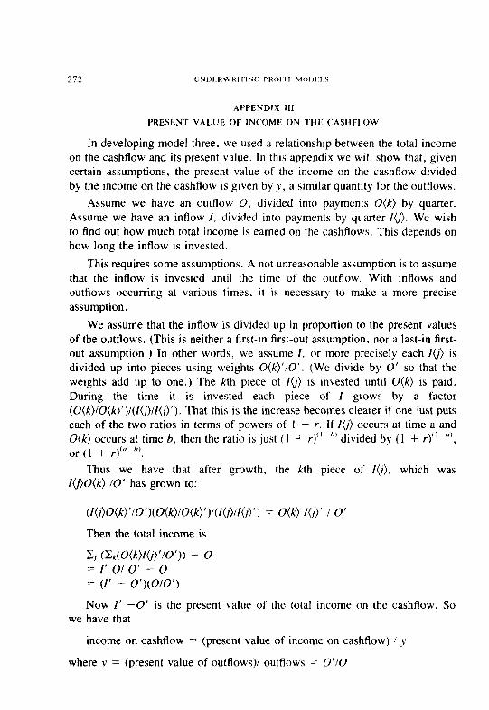
In developing model three, we used a relationship between the total income on the cashflow and its present value. In this appendix we will show that, given certain assumptions, the present value of the income on the cashflow divided by the income on the cashflow is given by y. a similar quantity for the outflows.

Assume we have an outflow 0, divided into payments O(k) by quarter. Assume we have an inflow I, divided into payments by quarter 1(j). We wish to find out how much total income is earned on the cashflows. This depends on how long the inflow is invested.

This requires some assumptions. A not unreasonable assumption is to assume that the inflow is invested until the time of the outflow. With inflows and outflows occurring at various times, it is necessary to make a more precise assumption.

We assume that the inflow is divided up in proportion to the present values of the outflows. (This is neither a first-in first-out assumption, nor a last-in first- out assumption.) In other words, we assume I, or more precisely each I(j) is divided up into pieces using weights O(k)‘iO’. (We divide by 0’ so that the weights add up to one.) The kth piece of f(j) is invested until O(k) is paid. During the time it is invested each piece of I grows by a factor (O(k)/O(k)‘)l(fg’)l~(j)‘)‘). That this is the increase becomes clearer if one just puts each of the two ratios in terms of powers of 1 + r. If f(j) occurs at time a and O(k) occurs at time 6, then the ratio is just ( 1 + r)“-” divided by (1 + r)(‘-“), or (1 + r)tu-h).

Thus we have that after growth, the kth piece of IO’). which was I(i)O(k)‘lO’ has grown to:

(I(i}O(k)‘/O’)(O(k)/O(k)‘)/(l(j)/lO’)’) = O(k) fO’)’ / 0’

Then the total income is

Cj (~~(O(k)f(j)‘/O’)) - 0 = 1’ 01 0’ - 0 = (I’ - O’)(O/O’)

Now I’ -0’ is the present value of the total income on the cashflow. So we have that

income on cashflow = (present value of income on cashflow) / y

where y = (present value of outflows)/ outflows = 0’10

UNDI~RWRITINC PHOFIl- b1OL~tI.S 273

APPENDIX IV

ALTERNATIVE TIMING OF NTf ON CASHFLOWS

In this appendix we will develop further the work done in the previous appendix. We will use the same notation. We will see how an alternate as- sumption concerning the timing of federal income taxes on the investment income on the cashflows yields a different result than in model three.

We saw how the krh piece of I@, which was t(i) O(k)‘lO’, grew to O(k)~(i)‘/O’. Thus the investment income is their difference

(O(k)lO’)’ - 1(j)O(k)‘)/O’

Let’s assume that the income taxes on this investment income are paid at time k. Then one gets this piece of the federal income taxes on investment by multiplying by FITI. Since the tax payment has been assumed to be made at time k, we get the present value by multiplying by a factor O(k)‘lO(k). Thus the present value of the federal income taxes on this piece of the investment income is

FfTl(O(k)‘lO(k))(O(k}l(i)’ - I(j)O(k)‘)/O’ = FITf(O(k)‘Io’)‘IO’ - Ig’)O(k)‘O(k)‘lO(k)O’)

When we sum over all i and j we get

PV(FITf on cashflows)lFlTt = I’ - (I/O’)(& O(k)‘O(k}‘lO(k))

This differs from model three where we had

PV(FlT1 on cashflows)lFlTI = y(I’y - I) = I’ - yi

If we define

z = (Ck O(k)‘O(k)‘lO(k))lO’

Then the result here can be rewritten as

PV(FITI on cashllows)lFITI = I’ - zl

This is of the exact same form as the result used in model three, except we have z in place of y. Thus the equation for P* would be the same, except we would replace y by z.

The resulting profit provisions are similar. For example, below are the results for the same numerical examples we calculated for model three, using the same inputs.

As Per This Appendix As Per Model Three

N(years) P* 2 Profit Prov. P* \ Profit Prov. - - L

.5 $1.044 I .060 3.4% $1.044 1.059 3.4% 1.0 979 1,021 - 1.7% 980 1.020 -1.6% 1.5 914 ,984 -7.5% 916 ,981 -7.3% 2.0 850 .948 - 14.2% 853 ,943 - 13.8%

UNDERWRI-l’lNC PROI‘ M0Dtl.S 275

APPENDIX V

DlFFERENTlATlON OF THE FORMULA FOR PROFIT PROVISION

In this appendix will be shown the manner in which the underwriting profit provision varies with various important inputs. This will be done by differen- tiating the formula for the underwriting profit provision. (In the main text were shown some actual numerical results of varying inputs.) We will use the third model.

u = 1 - t - (E + L)IP* = 1 - t - N/D

where N = (Y/S + g)( 1 - FIT!) - th - R/s + FlTly - (1 - t)FITUe and D = (L’ + E’)I(L + E) - FtTUe (N and D have been used for numerator and denominator, only in this appendix.)

Then we have

duidR = I/SD

Thus, duldR is greater than zero, and is approximately 1 for the values used here.

dulds = (r(l - FITI) - R)lDs2

Thus, duids is less than zero and is approximately -.05 for the values used here.

duldFITU = (1 - t)elD - eNID = e( 1 - t)/D - e( 1 - u - t)/D = eulD

Thus, duldFITU has the same sign as u, and is approximately equal to 2~4.

duldFITI = (r/s + g - y)lD

Thus, duldFIT1 is generally greater than zero. It is significantly larger the longer the cashflows.

The reason we don’t give an algebraic result for duldr is that the result of differentiating u by r would be quite a complex expression. Remember that variables which involve present values, such as g, h, y, E’, and L’, involve r, in a rather complicated manner.

APPENDIX VI

INVESTMENT BALANCE FOR TAXES

In this appendix we will explore an alternate way to get the expression for the present value of the taxes on investment income on the cashflow, which was used in the third model. We will set up something called the investment balance for taxes, IBT for short.

Assume there is an inflow I(j) and outflow O(j), each by quarter. Call the sums I and 0. Deal with I(i> and O(i>I/O, so that both vectors sum to the same value I. (Think of I as the premiums loaded for profits. Intuitively this manner of doing things prevents counting the underwriting profit or loss twice, since it is dealt with separately elsewhere in the model.)

Let No) = IQ) - Olj)IlO. N is the net cashflow by quarter, but adjusted so that the outflows are loaded for profit.

Then the IBT is set up as follows. Take the cumulative sum by quarter of N. (Since we have set them up so that both vectors have the same sum, for large enough values of time IBT is 0.) lBT(j) = Ck-1 ,,> j N(k), Then in each quarter this amount is available to earn investment income. So we multiply it by y = (I + r).” - 1, the quarterly rate of investment return. Assume the income taxes are paid on this investment income the following quarter. Assume for convenience that the first element of the vectors has a discount factor of 1. (One can discount to any point in time. If another point in time is taken, an additional discount factor will appear. but make no difference in the result.)

PV(qIBT)FITI( 1 + r)-.2s = FITIq (E, &= 1 to, (N(k) (1 + r)- “‘))

Now collect all the terms involving a given NO’). Each NO’) appears starting with a term in which it is multiplied by a factor of (1 + r)-“*. Then it appears in all the subsequent terms, except in the next term it is multiplied by (I + r)-(J+i)‘4, in the one after that by (I + r) ~oc2)‘4, etc. Thus,

= FITIq (2, (N(j) C,=, I,, r (I + r))“‘))

Now take the sum of the infinite geometric series.

= FITIq 2, NO’)( I + r)-J’4/( I - ( 1 + r) “) = FITI EJ N(j)q( I + r)-J’4/q( I + r)- 2s = FITI 2, NG)(l + r)plrp’)‘4

UNDERWRITING PROI’I I MOl>tl.S 277

But we have assumed for convenience that the N(1) term has its present value given by a discount factor of 1. Each subsequent term of N(j) has an additional factor of (1 + r)“4 in order to get its present value, since it is one quarter later. Thus,

= FITI Cj PV(N(j)) = FITI (I’ - O’IIO)

What we use in model three is

FITI (P*’ - L’ -E’ -p’ - #* _ L’ - E’ -7-e’))

= FITI(I’ - 0’ -y(l - 0)) = FITI(I’ - 0’ -(O’lO)(I - 0)) = FITI(I’ - O’IIO)

This is the same result as we got using the ZBT method here.