Embed Size (px)
Citation preview

An Introduction to the General Number Field Sieve
Matthew E. Briggs
Thesis submitted to the Faculty of theVirginia Polytechnic Institute and State University
in partial fulfillment of the requirements for the degree of
Master of Sciencein
Mathematics
Dr. Ezra Brown, ChairDr. Martin Day
Dr. Charles Parry
April 17, 1998Blacksburg, Virginia
Keywords: Number Field Sieve, Factoring, Cryptography, Algebraic Number TheoryCopyright 1998, Matthew E. Briggs

An Introduction to the General Number Field Sieve
Matthew E. Briggs
(ABSTRACT)
With the proliferation of computers into homes and businesses and the explosive growth rateof the Internet, the ability to conduct secure electronic communications and transactions hasbecome an issue of vital concern. One of the most prominent systems for securing electronicinformation, known as RSA, relies upon the fact that it is computationally difficult to factora “large” integer into its component prime integers. If an efficient algorithm is developedthat can factor any arbitrarily large integer in a “reasonable” amount of time, the securityvalue of the RSA system would be nullified.
The General Number Field Sieve algorithm is the fastest known method for factoring largeintegers. Research and development of this algorithm within the past five years has facili-tated factorizations of integers that were once speculated to require thousands of years ofsupercomputer time to accomplish. While this method has many unexplored features thatmerit further research, the complexity of the algorithm prevents almost anyone but an expertfrom investigating its behavior. We address this concern by first pulling together much ofthe background information necessary to understand the concepts that are central in theGeneral Number Field Sieve. These concepts are woven together into a cohesive presenta-tion that details each theory while clearly describing how a particular theory fits into thealgorithm. Formal proofs from existing literature are recast and illuminated to clarify theirinner-workings and the role they play in the whole process. We also present a complete,detailed example of a factorization achieved with the General Number Field Sieve in orderto concretize the concepts that are outlined.

Contents
1 Introduction 1
1.1 Cryptography and Factoring . . . . . . . . . . . . . . . . . . . . . . . . . . . 2
1.2 Modern Methods of Factoring . . . . . . . . . . . . . . . . . . . . . . . . . . 3
1.3 The Quadratic Sieve . . . . . . . . . . . . . . . . . . . . . . . . . . . . . . . 5
2 Motivation for the General Number Field Sieve 7
2.1 Generalizing the Quadratic Sieve . . . . . . . . . . . . . . . . . . . . . . . . 8
2.2 Fields and Roots of Irreducible Polynomials . . . . . . . . . . . . . . . . . . 8
2.3 Rings of Algebraic Integers . . . . . . . . . . . . . . . . . . . . . . . . . . . . 10
2.4 Producing a Difference of Squares . . . . . . . . . . . . . . . . . . . . . . . . 10
3 The General Number Field Sieve Algorithm 12
3.1 Smoothness And The Algebraic Factor Base . . . . . . . . . . . . . . . . . . 13
3.2 Quadratic Characters . . . . . . . . . . . . . . . . . . . . . . . . . . . . . . . 20
3.3 Summary of Finding Squares in Z [θ] . . . . . . . . . . . . . . . . . . . . . . 22
3.4 The Rational Factor Base and Sieving . . . . . . . . . . . . . . . . . . . . . 23
3.5 Speeding Up The Sieve . . . . . . . . . . . . . . . . . . . . . . . . . . . . . . 24
3.6 Implementation Techniques For Speeding Up The Sieve . . . . . . . . . . . . 24
3.7 Sieving with the Algebraic Factor Base . . . . . . . . . . . . . . . . . . . . . 25
3.8 An Implementation Note . . . . . . . . . . . . . . . . . . . . . . . . . . . . . 26
4 Filling in the Details 27
iii
4.1 Finding a Polynomial . . . . . . . . . . . . . . . . . . . . . . . . . . . . . . . 28
4.2 Finding First Degree Prime Ideals of Z [θ] . . . . . . . . . . . . . . . . . . . . 29
4.3 Matrices and Dependencies . . . . . . . . . . . . . . . . . . . . . . . . . . . . 30
4.4 The Lanczos Algorithm . . . . . . . . . . . . . . . . . . . . . . . . . . . . . . 32
4.5 Lanczos in Practice . . . . . . . . . . . . . . . . . . . . . . . . . . . . . . . . 37
4.6 Computing φ(β) When β2 ∈ Z [θ] is Known . . . . . . . . . . . . . . . . . . . 39
4.7 Finite Fields and Q (θ) . . . . . . . . . . . . . . . . . . . . . . . . . . . . . . 40
4.8 Computing Square Roots in F pd . . . . . . . . . . . . . . . . . . . . . . . . . 45
4.9 Irreducibility Testing of Polynomials Modulo p . . . . . . . . . . . . . . . . . 48
5 An Extended Example 51
5.1 Selecting the Polynomial . . . . . . . . . . . . . . . . . . . . . . . . . . . . . 51
5.2 The Rational Factor Base . . . . . . . . . . . . . . . . . . . . . . . . . . . . 52
5.3 The Algebraic Factor Base . . . . . . . . . . . . . . . . . . . . . . . . . . . . 52
5.4 The Quadratic Character Base . . . . . . . . . . . . . . . . . . . . . . . . . . 53
5.5 Sieving . . . . . . . . . . . . . . . . . . . . . . . . . . . . . . . . . . . . . . . 54
5.6 Forming the Matrix . . . . . . . . . . . . . . . . . . . . . . . . . . . . . . . . 55
5.7 Finding Dependencies . . . . . . . . . . . . . . . . . . . . . . . . . . . . . . 57
5.8 Computing An Explicit Square Root in Z [θ] . . . . . . . . . . . . . . . . . . 57
5.9 Determining Applicable Finite Fields . . . . . . . . . . . . . . . . . . . . . . 58
5.10 Square Roots in a Finite Field . . . . . . . . . . . . . . . . . . . . . . . . . . 59
5.11 Using the Chinese Remainder Theorem . . . . . . . . . . . . . . . . . . . . . 60
5.12 Putting It All Together . . . . . . . . . . . . . . . . . . . . . . . . . . . . . . 62
6 Polynomial Selection and Parameter Tuning 63
6.1 Tweaking the Base-m Method . . . . . . . . . . . . . . . . . . . . . . . . . 63
6.2 Using Polynomials of the Formf(x) + g(x) . . . . . . . . . . . . . . . . . . . 64
6.3 Finding a Good Polynomial . . . . . . . . . . . . . . . . . . . . . . . . . . . 64
6.4 Example Polynomial Selection . . . . . . . . . . . . . . . . . . . . . . . . . . 65
iv

6.5 Testing the Example Polynomials . . . . . . . . . . . . . . . . . . . . . . . . 66
6.6 The Guessing Game . . . . . . . . . . . . . . . . . . . . . . . . . . . . . . . 67
6.7 An Alternate Strategy . . . . . . . . . . . . . . . . . . . . . . . . . . . . . . 68
A Example Performance Data 69
v

List of Tables
1.1 Scenarios for x2 ≡ y2 (mod n) . . . . . . . . . . . . . . . . . . . . . . . . . . 4
5.1 Rational Factor Base For n = 45, 113 . . . . . . . . . . . . . . . . . . . . . . 52
5.2 Algebraic Factor Base For n = 45, 113 . . . . . . . . . . . . . . . . . . . . . . 54
5.3 Quadratic Character Base For n = 45, 113 . . . . . . . . . . . . . . . . . . . 54
5.4 (a, b) Pairs Found During Sieving . . . . . . . . . . . . . . . . . . . . . . . . 55
5.5 (a, b) Pairs Occurring In a Dependency . . . . . . . . . . . . . . . . . . . . . 57
5.6 Primes Determining Finite Fields F p3i
. . . . . . . . . . . . . . . . . . . . . . 59
5.7 Members of S8 and Their Squares . . . . . . . . . . . . . . . . . . . . . . . . 60
5.8 Square Roots of δ in Finite Fields . . . . . . . . . . . . . . . . . . . . . . . . 61
A.1 f1(x) with small factor base . . . . . . . . . . . . . . . . . . . . . . . . . . . 69
A.2 f1(x) with medium factor base . . . . . . . . . . . . . . . . . . . . . . . . . . 69
A.3 f1(x) with large factor base . . . . . . . . . . . . . . . . . . . . . . . . . . . 70
A.4 f2(x) with small factor base . . . . . . . . . . . . . . . . . . . . . . . . . . . 70
A.5 f2(x) with medium factor base . . . . . . . . . . . . . . . . . . . . . . . . . . 70
A.6 f2(x) with large factor base . . . . . . . . . . . . . . . . . . . . . . . . . . . 71
A.7 f3(x) with small factor base . . . . . . . . . . . . . . . . . . . . . . . . . . . 71
A.8 f3(x) with medium factor base . . . . . . . . . . . . . . . . . . . . . . . . . . 71
A.9 f3(x) with large factor base . . . . . . . . . . . . . . . . . . . . . . . . . . . 72
A.10 f4(x) with small factor base . . . . . . . . . . . . . . . . . . . . . . . . . . . 72
A.11 f4(x) with medium factor base . . . . . . . . . . . . . . . . . . . . . . . . . . 72
vi

A.12 f4(x) with large factor base . . . . . . . . . . . . . . . . . . . . . . . . . . . 73
vii
Chapter 1
Introduction
The General Number Field Sieve (GNFS) is the fastest known method for factoring “large”integers, where large is generally taken to mean over 110 digits. This makes it the best algo-rithm for attempting to unscramble keys in the RSA [2, Chapter 4] public-key cryptographysystem, one of the most prevalent methods for transmitting and receiving secret data. Infact, GNFS was used recently to factor a 130-digit “challenge” number published by RSA,the largest number of cryptographic significance ever factored.
A specialized version of GNFS, the so-called “special” Number Field Sieve (SNFS), alsoexists; it is asymptotically faster than GNFS for factoring integers expressible in the formre ± s with r, e, s ∈ Z and e > 0. This has made SNFS the method of choice for attackingand successfully factoring the 155-digit ninth Fermat number [18], 229
+ 1, as well as forfactoring Mersenne “primes” and numbers on the Cunningham List [3], the latter being oneof the oldest gauges of factoring technology.
Beyond its practical value, GNFS is also academically interesting. The algorithm itself usesideas and results from diverse fields of mathematics and computer science. Algebraic numbertheory, graph theory, finite fields, linear algebra, and even real and complex analysis all playvital roles in GNFS.
The goal here is to describe the basic GNFS algorithm, explaining the relevant backgroundinformation and theory the reader will need in order to understand the various stages ofGNFS. We’ll spend considerable time on an extended example, worked out in full detailso as to provide the reader a clear grasp of the previously outlined concepts. Once thefundamentals have been laid, we’ll describe practical use of GNFS. This includes details ontuning GNFS for specific situations, as well as some of the general enhancements made tothe base algorithm that improve its performance.
1

Matthew E. Briggs Chapter 1. Introduction 2
1.1 Cryptography and Factoring
Most cryptography systems make use of “one-way” functions, which intuitively can bethought of as mappings that are difficult to invert. In the RSA system [2, Chapter 4]the one-way function is multiplication of large prime integers, where large usually meansover 110 digits. The key is that while multiplication of such integers can be done nearlyinstantly, the inversion function of factoring back into primes is virtually impossible.
In many of these systems, including the RSA procedure, an individual who wants the abilityto receive encrypted messages that only he can read chooses a “public key” and a “privatekey.” The public key is available to anyone and is used to encrypt messages that can onlybe decrypted by someone who knows the corresponding private key. RSA facilitates thisconcept by having the private key consist of a set of three integers p, q, and d. The integersp and q are chosen to be large primes such that their product n = p · q is difficult to factor,while d is chosen relatively prime to φ(n), where φ(n) denotes Euler’s totient function forthe number of integers less than or equal to n and relatively prime to n. The public key iscomprised of the integer n and the integer e for which d · e ≡ 1 (mod φ(n)).
To encrypt a message using the integers n and e for a public key, first encode the message [2,Chapter 4] as an integer M relatively prime to n. Let E denote the encrypted version of themessage, where E is defined as
E = Me (mod n).
This integer E can be made available to anyone but it can only be decrypted back into theoriginal message M by someone knowing the corresponding private key.
To decrypt the message, recall Euler’s formula [24, Theorem 2.8] which says that for anyintegers m and a with gcd(a,m) = 1 that aφ(m) ≡ 1 (mod m). Since M was chosen relativelyprime to n it follows then that Mφ(n) ≡ 1 (mod n). Using this information leads to a methodfor decrypting E, since
Ed ≡ (Me)d ≡Med ≡M1+k·φ(n) ≡M · (Mφ(n))k ≡M (mod n)
where ed = 1 + k · φ(n) for some integer k since d · e ≡ 1 (mod φ(n)) by construction.Note this computation recovers the original message M and makes use of information in theprivate key set.
To make clear the importance of factoring n, note that to decrypt the message the privatekey d was needed. Now e and n are in the public key set, and it is known that d · e ≡ 1(mod φ(n)), so d can be computed by computing the multiplicative inverse of e moduloφ(n). The latter is trivial, assuming φ(n) is known. Now from [24, Theorem 2.19]
φ(n) = φ(pq) = φ(p) · φ(q) = (p− 1) · (q − 1)
which is not immediately computable unless p and q are available. The latter is not a problemfor someone with knowledge of the private key set, but for anyone else it entails factoring
Matthew E. Briggs Chapter 1. Introduction 3
n. Furthermore, if a method for computing φ(n) without knowing p or q is discovered, thenn can be factored immediately. So the problem of unearthing the private key d boils downto computing φ(n), which in turn is equivalent to factoring n. If a method is discovered forfactoring arbitrary integers quickly, then any RSA private key could be discovered and thesystem would become insecure.
1.2 Modern Methods of Factoring
The most straightforward method of factoring is trial division, where one simply tries todivide by each prime up to the square root of the number to factor. This method is in-deed guaranteed to find a factor of any composite integer, but it is also guaranteed to becomputationally infeasible for large enough integers.
To see why this is the case, suppose a 60-digit integer n is to be factored. Then one must checkif n is divisible by any of the primes of size up to about 1030. If the optimistic assumption ismade that only 0.1% of these integers are prime, that still means about 1027 divisions needto take place. Again, being optimistic and assuming that enough computer resources areavailable to do 1015 of these divisions every second, it would still take roughly 1012 seconds,or over 31, 000 years to perform the computation. Of course, the algorithm might find afactor of n without extending all the way to the square root of n, so it may very well take afew thousand years less. On the other hand, the assumptions made were fairly optimistic tobegin with so the algorithm would probably take longer than this rough projection. In anyevent, this obviously is not a practical method for factoring with run-times in the thousandsof years!
Many of the successful factoring methods of the past twenty years have used the same basictechnique, which itself dates back to the time of Fermat [26, 2]. The “difference of squares”method relies upon the observation that if integers x and y are such that x 6≡ y (mod n)and
x2 ≡ y2 (mod n) (1.1)
then gcd(x− y, n) and gcd(x+ y, n) are non-trivial factors of n.
If one is able to produce random integers x and y that satisfy (1.1), how likely is it thatgcd(x+ y, n) or gcd(x− y, n) is a non-trivial factor of n? In the case where n is the productof two distinct primes p and q, such as when n is a modulus used in the RSA method of§1.1, it turns out that a non-trivial factor of n is extracted in 2/3 of the cases, as seen inTable 1.1.
The question then becomes one of devising a means for producing integers x and y satisfying(1.1). The “random squares” algorithm of Dixon is one such method, which is not only ofhistorical interest, but is also useful because it introduces concepts employed in the GNFS.Specifically, the notions of a factor base and being smooth over a factor base are introduced:

Matthew E. Briggs Chapter 1. Introduction 4
Table 1.1: Scenarios for x2 ≡ y2 (mod n)p|x+ y? p|x − y? q|x+ y? q|x− y? gcd(x+ y, n) gcd(x− y, n) Gives Factor?
Yes Yes Yes Yes n nYes Yes Yes No n p XYes Yes No Yes p n XYes No Yes Yes n q XYes No Yes No n 1Yes No No Yes p q XNo Yes Yes Yes q n XNo Yes Yes No q p XNo Yes No Yes 1 n
Definition 1.2.1. A nonempty set F of positive prime integers is called a factor base. Aninteger k is said to be smooth over the factor base F if all primes occurring in the uniquefactorization of k into primes are members of F .
The method of Dixon [2, pages 102–104] begins by fixing a factor base F = {p1, p2, . . . , pm}and then proceeds to compute a set of random integers ri with the property that f(ri) = r2
i
(mod n) is smooth over F . When more than m such integers are found, a subset U of theintegers in the sequence can be found such that∏
ri∈Uf(ri) = p2e1
1 p2e22 · · · p2em
m = (pe11 pe22 · · · pemm )2
with ei ≥ 0. This set U is the key to producing a difference of squares, for if
x =∏ri∈U
ri and y = pe11 pe22 · · · pemm
then a difference of squares follows from
x2 =∏ri∈U
r2i ≡
∏ri∈U
f(ri) ≡ y2 (mod n).
Finding the set U turns out to be a reasonably straightforward task. For each ri ∈ U one canassociate a vector vi ∈ Fm2 , where Fm2 denotes the m-dimensional vector space over the finite
field Z /2Z of 2 elements. The jth coordinate of vi is set to 0 if the prime pj divides f(ri) aneven number of times and is set to 1 otherwise. It’s a standard result from linear algebra [11,Theorem 1.10] that if more than m such vectors are collected then there is a non-trivial lineardependence among them. In this particular case, that means a nonempty set of vi vectorscan be produced whose sum yields the zero vector. But since these vectors represent theparity of the exponents of the primes that occur in the factorization of the f(ri)’s, it follows
Matthew E. Briggs Chapter 1. Introduction 5
that the product of the f(ri) values corresponding to the vi’s that occur in a dependency isa perfect square. The set U can then be constructed from the ri whose vector vi occurs in adependency. Many well-studied and efficient techniques exist for finding dependencies amongvectors, such as Gaussian elimination [2, pages 114–115]. The real question then becomesone of finding enough ri with f(ri) smooth over F , and doing so in a timely fashion..
1.3 The Quadratic Sieve
The Quadratic Sieve (QS) factoring algorithm of Carl Pomerance [26, 2] was the most ef-fective general-purpose factoring algorithm of the 1980’s and the early 90’s, and is still themethod of choice for integers between 50 and 100 digits. At its heart the QS is essentiallyDixon’s algorithm, in the sense that it uses factor bases, smoothness, and dependenciesamong vectors over Z /2Z to produce its squares. Through a slight modification of thepolynomials f(x) considered, however, QS sets itself apart from Dixon’s method by findingsmooth values in a remarkably fast manner.
As with Dixon’s method, QS begins by fixing a factor base F = {p1, p2, . . . , pm}. Instead ofsearching for integers ri for which f(ri) = r2
i (mod n) is smooth over F , values of f(ri) =r2i − n are sought which are smooth over F . Again, as is the case in Dixon’s method, when
more than m such integers are found, a subset U can be produced with∏ri∈U
f(ri) = p2e11 p2e2
2 · · · p2emm = (pe11 p
e22 · · · pemm )2.
A difference of squares follows by letting
x =∏ri∈U
ri and y = pe11 pe22 · · · pemm
since then
x2 =∏ri∈U
r2i ≡
∏ri∈U
(r2i − n) ≡
∏ri∈U
f(ri) ≡ y2 (mod n). (1.2)
At this point the QS does not look that much different from Dixon’s algorithm, and in realityit is not. The only difference is in the polynomial f(ri) = r2
i − n used, and in fact it is thespecial form of this polynomial that allows the dramatic increase in speed alluded to earlier.
The big improvement comes in how the different ri are chosen when considering whetherf(ri) is smooth over F . The straightforward approach is to pick a random integer ri andthen to trial-divide f(ri) by the primes in F . If f(ri) factors completely over F then ri isadded to the set of “useful” ri, otherwise it is discarded. In either case, a new random riis picked and the process continues until more than m integers exist in the set of useful rivalues.
Matthew E. Briggs Chapter 1. Introduction 6
The problem with this approach is that a lot of time is wasted attempting to divide by primesin F that don’t evenly divide a particular f(ri). A dramatic improvement can be made bychanging the focus of the operations. Instead of concentrating on a fixed f(ri) and findingout which primes in the factor base divide it, fix a prime p ∈ F and determine which f(ri)values are divisible by that p. If determining the f(ri) values that are divisible by a fixedprime p ∈ F can be done in a reasonable manner, then one saves the time of attempting todivide by primes that don’t divide into an f(ri).
To see how the special form of f(ri) = r2i − n facilitates this, fix an ri and a prime p ∈ F
and suppose p divides f(ri). Then f(ri) ≡ 0 (mod p) and hence r2i − n ≡ 0 (mod p) by the
definition of the function f . Then for any integer k it follows that
f(ri + kp) = r2i + 2rikp+ k2p2 − n ≡ r2
i − n ≡ 0 (mod p)
and hence p divides f(ri + kp) as well. Thus, the real work in finding values of ri for whichf(ri) is divisible by p amounts to initially solving the quadratic congruence r2
i ≡ n (mod p),for which there is an easy and efficient method [16, Section 9.2]. The rest of the ri values forwhich f(ri) is divisible by p are then ri + pk for k ∈ Z . In order for this procedure to work,n must be a quadratic residue modulo p, hence F shouldn’t contain any primes for which nis a quadratic non-residue.
In practice one selects a bound −u < ri < u on the ri values for which it is expected morethan m of the possible values of f(ri) within this range will be smooth over F . An array ofcomputer memory is then initialized to the f(ri) values within this range. For each primep ∈ F , the quadratic congruence r2
i ≡ n (mod p) is solved. Then for all integers k for which−u < ri + pk < u, the prime p is divided out of the corresponding f(ri + pk) value. Finally,after this procedure has been performed for every prime p, the array of computer memory isscanned for values of f(ri) for which f(ri) = 1. These correspond to values of ri whose f(ri)factor completely over the factor base.
Using this sieving technique, every division by a prime p is “useful” in the sense that it isalways guaranteed to divide into the f(ri) value that is selected, which is not the case at allwith blind trial division. Since division is one of the most time-consuming operations in acomputer, this shift in focus leads to a dramatic speed-up.
Chapter 2
Motivation for the General NumberField Sieve
Almost all difference of squares methods that produce integers x and y as in (1.1) use thesame basic concepts of a factor base, smoothness, and finding dependencies among vectorsover Z /2Z . Key breakthroughs occur when new methods are developed or older methodsenhanced to produce more smooth values over a factor base in a time dramatically less thanprevious methods. For instance, Dixon’s method is improved upon by QS by adjusting thepolynomials that are used, and more importantly by changing the perspective on how smoothvalues are searched for. This latter shift in perspective facilitates a fast sieving procedurefor finding smooth values, and hence a breakthrough in factoring technology.
The ideas leading to the GNFS algorithm are motivated by similar techniques that led tothe development of the QS from Dixon’s method. As expected, then, the notions of a factorbase, smoothness and dependency-finding are used in the GNFS, along with a perspective forfinding smooth values that supports a sieving procedure. A big break through comes by firstrealizing that the quadratic polynomials of Dixon’s method and the QS don’t necessarily haveto be quadratic. Perhaps certain cubic, quartic, quintic, or even higher degree polynomialscould produce more smooth values than quadratics.
Another less obvious improvement stems from somehow allowing other rings besides Z andZ /nZ into the algorithm. The idea here is that other rings could potentially have a notionof smoothness imposed on them, similar to the notion over Z , with the hopes that moresmooth values exist in such rings than in Z . Furthermore, if some kind natural mappingexisted between such rings and Z /nZ , then a way of producing a difference of squares couldpossibly be arrived at.
This idea of using other rings to produce a difference of squares is explored in §2.1 and thentied in with higher degree polynomials in §2.2, §2.3, and §2.4.
7
Matthew E. Briggs Chapter 2. Motivation for the General Number Field Sieve 8
2.1 Generalizing the Quadratic Sieve
To see how rings other than Z and Z /nZ can come into play in a difference of squaresmethod, one only has to generalize the role the polynomial f(ri) = r2
i − n plays in the QS.Recall from §1.3 that in the QS a set of integers U is found such that (1.2) holds. Then thepolynomial f(ri) = r2
i − n can be thought of as a ring homomorphism f : Z → Z /nZ . Inparticular, f maps the product of all f(ri) for ri ∈ U , which is smooth over the factor baseF (by the choice of the ri) and a perfect square in Z (by the definition of U), to a perfectsquare in Z /nZ . The important point is that f maps a square in the ring Z to a square inthe ring Z /nZ , which supplies the integers x and y for (1.1).
Suppose that there exists a ring R and a ring homomorphism φ : R→ Z /nZ . If β ∈ R withφ(β2) = y2 (mod n) and x = φ(β) (mod n) then
x2 ≡ φ(β)2 ≡ φ(β2) ≡ y2 (mod n).
So if an element in R can be found that is a perfect square in R and which maps to aperfect square in Z /nZ , then applying φ will yield a difference of squares. As will be seen inthe following sections, there is a natural way to construct such rings and the correspondinghomomorphisms to Z /nZ that will yield a difference of squares.
2.2 Fields and Roots of Irreducible Polynomials
Suppose a monic, irreducible polynomial f(x) of degree d with rational coefficients is known.Then f(x) splits into distinct linear factors over the complex numbers [10, Section 13.4] as
f(x) = (x− θ1)(x− θ2) · · · (x− θd)
with θi ∈ C . One can choose any root θ = θi and form a ring in a manner that is easy toverify [14, Chapter 5, Theorem 1.3]:
Proposition 2.2.1. If θ denotes a complex root of a monic, irreducible polynomial f(x) withrational coefficients, then the set of all polynomials in θ with rational coefficients, denotedQ (θ), forms a ring.
In fact, much more is true of Q (θ) because of the monic, irreducible nature of the definingpolynomial f(x):
Theorem 2.2.2. Given a monic, irreducible polynomial f(x) with rational coefficients, aroot θ ∈ C of f(x), and the associated ring Q (θ), the following hold:
1. Q (θ) ∼= Q [x]/(f(x)).

Matthew E. Briggs Chapter 2. Motivation for the General Number Field Sieve 9
2. Q (θ) is a field.
3. f(x) divides any polynomial g(x) for which g(θ) = 0.
4. The set {1, θ, θ2, . . . , θd−1} forms a basis for Q (θ) as a vector space over Q .
Proof. Proceeding along the lines of [14, Chapter 5, Theorem 1.6], let φ : Q [x] → Q (θ)denote the natural map with φ(Q ) = Q and φ(x) = θ, which maps polynomials in x topolynomials in θ. It is clear that this mapping is actually a surjective ring homomorphism.Now f(x) maps to f(θ) = 0 under the mapping φ so that f(x) ∈ kerφ. In fact, since Q is afield it follows that Q [x] is a principal ideal domain [14, Chapter 3, Theorem 3.9] and hencekerφ = (g(x)) for some polynomial g(x). Now f(x) ∈ kerφ = (g(x)) implies that f(x) is amultiple of g(x), and since f(x) is irreducible is follows that g(x) and f(x) must differ by atmost a scalar so that kerφ = (g(x)) = (f(x)). Now Q [x]/kerφ ∼= Imφ and since φ is onto itfollows that Q [x]/(f(x)) ∼= Q (θ) and the first part of the theorem follows.
To prove the second condition, note (0) $ (f(x)) $ Q [x] since f(x) is not identically 0 andkerφ = (f(x)) is not the whole ring Q [x] because φ maps the non-zero rationals to non-zerorationals. Since f(x) is irreducible it follows [29, Proposition 4.4] that (f(x)) is maximalwith respect to all proper principal ideals of Q [x]. But Q [x] is a principal ideal domain andhence (f(x)) is a maximal ideal of Q [x]. Thus Q [x]/(f(x)) ∼= Q (θ) is a field [29, Lemma 5.1].
For the third part, consider a polynomial g(x) for which g(θ) = 0. Then φ(g(x)) = g(θ) = 0implies that g(x) ∈ kerφ and since kerφ = (f(x)) it follows that g(x) is a multiple of f(x).
Finally, to prove the result about a representation for Q (θ) as a vector space over Q , letg(θ) ∈ Q (θ) be any polynomial in θ and g(x) ∈ Q [x] its corresponding representation as apolynomial in x. By the division algorithm, g(x) may be written as
g(x) = q(x) · f(x) + r(x)
where deg r(x) < deg f(x). Then
g(θ) = q(θ) · f(θ) + r(θ) = q(θ) · 0 + r(θ) = r(θ)
since θ is a root of f(x). It follows then that g(θ) may be written in the form
g(θ) = ad−1θd−1 + ad−2θ
d−2 + a1θ + a0
where the ai ∈ Q are the coefficients of r(x), since r(x) is a polynomial of degree strictlyless than d. Thus the set {1, θ, θ2, . . . , θd−1} spans Q (θ) as a vector space over Q . To showlinear independence, suppose that ad−1θd−1 + ad−2θd−2 + · · ·+ a1θ+ a0 = 0. Letting g(x) bethe polynomial
g(x) = ad−1xd−1 + ad−2x
d−2 + · · ·+ a1x+ a0
it follows by construction that g(θ) = 0. Thus, g(x) ∈ kerφ = (f(x)) and hence f(x) mustdivide g(x). But the degree of f(x) is strictly greater than g(x) so that g(x) must be thezero polynomial and hence ai = 0 for all 0 ≤ i < d and linear independence follows.
Matthew E. Briggs Chapter 2. Motivation for the General Number Field Sieve 10
2.3 Rings of Algebraic Integers
At this point, to summarize the important developments, we have shown that a monic,irreducible polynomial f(x) of arbitrary degree d and with rational coefficients gives rise toa field Q (θ) where θ ∈ C is a root of f(x). Furthermore, elements of Q (θ) can be convenientlyrepresented as Q -linear combinations of the elements S = {1, θ, θ2, . . . , θd−1}. Although thelatter representation is convenient, working with Z -linear combinations of the elements of Swould be easier since then denominators could be discounted. Further analysis of the fieldQ (θ) turns up a ring whose elements can be represented in just such a manner.
Definition 2.3.1. A complex number α is called an algebraic integer if it is the root of amonic polynomial with integer coefficients.
Thus, if f(x) is an irreducible, monic polynomial of degree d with integer coefficients andθ ∈ C is a root of f(x), it follows that θ is an algebraic integer according to this definition.The following is a standard result from algebraic number theory that justifies the definition:
Proposition 2.3.1. Given a monic, irreducible polynomial f(x) of degree d with rationalcoefficients and a root θ ∈ C of f(x), the set of all algebraic integers in Q (θ), denoted O,forms a subring of the field Q (θ).
The actual ring that will be used in the GNFS is subring of the ring of algebraic integers O ofQ (θ) which possesses the convenient representation mentioned in the beginning paragraph:
Proposition 2.3.2. Given a monic, irreducible polynomial f(x) of degree d with integercoefficients and a root θ ∈ C of f(x), the set of all Z -linear combinations of the elements{1, θ, θ2, . . . , θd−1}, denoted Z [θ], forms a subring of the ring of algebraic integers O of Q (θ).
Before going further, it should be pointed out that the subring Z [θ] can indeed be a propersubring of O. For instance, the polynomial x2− 5 is easily seen to be irreducible and monicso that Q
(√5)
forms a field, which is a vector space over Q with basis S ={
1,√
5}
. If
α =(1 +√
5)/2 then α ∈ Q
(√5)
since α is a Q -linear combination of the elements of S.Furthermore α satisfies the polynomial g(x) = x2 − x− 1 and is hence an algebraic integer,but clearly α 6∈ Z [θ]. Hence, Q
(√5)
possesses an algebraic integer which is not contained
in Z[√
5]
and so
Z[√
5]$ O $ Q
(√5).
2.4 Producing a Difference of Squares
Having demonstrated that for any monic, irreducible polynomial an associated ring can beconstructed that has a natural representation as Z -linear combinations of elements from

Matthew E. Briggs Chapter 2. Motivation for the General Number Field Sieve 11
a finite set, the natural question is how to map that ring onto Z /nZ so as to produce adifference of squares. The next proposition [5, page 53] addresses this issue:
Proposition 2.4.1. Given a monic, irreducible polynomial f(x) with integer coefficients, aroot θ ∈ C of f(x), and an integer m ∈ Z /nZ for which f(m) ≡ 0 (mod n), the mappingφ : Z [θ] → Z /nZ with φ(1) = 1 (mod n) and which sends θ to m is a surjective ringhomomorphism.
To see how this can result in a difference of squares, suppose a set U of pairs of integers(a, b) can be found such that∏
(a,b)∈U
(a+ bθ) = β2 and∏
(a,b)∈U
(a+ bm) = y2
with β ∈ Z [θ] and y ∈ Z . Then applying the natural homomorphism φ from Proposition 2.4.1and letting φ(β) = x ∈ Z /nZ , it follows that
x2 ≡ φ(β)2 ≡ φ(β2) ≡ φ
∏(a,b)∈U
(a+ bθ)
≡
∏(a,b)∈U
φ(a+ bθ) ≡∏
(a,b)∈U
(a+ bm) ≡ y2 (mod n)
and a difference of squares results.
Note 2.4.1. The condition that the product of the elements a+ bθ corresponding to pairs inU be a perfect square in Z [θ] is imposed because the ring homomorphism φ is only definedon elements of Z [θ]. In practice the condition is relaxed to allow for the product being aperfect square in Q (θ), which is less restrictive and hence more likely to be satisfied. Now if∏
(a,b)∈U
(a+ bθ) = α2 (2.1)
for some α ∈ Q (θ), it follows [5, pages 60–61] that α ∈ O and in fact f ′(θ) · α ∈ Z [θ]. Adifference of squares can still be produced, for if∏
(a,b)∈U
(a+ bθ) = α2 and∏
(a,b)∈U
(a+ bm) = z2 (2.2)
with α ∈ O and z ∈ Z , then letting β = f ′(θ) ·α ∈ Z [θ], y = f ′(m) ·z, and x = φ(β) ∈ Z /nZ ,it follows that
x2 ≡ φ(β)2 ≡ φ(β2) ≡ φ
f ′(θ)2 ·∏
(a,b)∈U
(a+ bθ)
≡ φ (f ′(θ))2 ·
∏(a,b)∈U
φ(a+ bθ) ≡ f ′(m)2 ·∏
(a,b)∈U
(a+ bm) ≡ y2 (mod n)
and another difference of squares has been produced.
Chapter 3
The General Number Field SieveAlgorithm
In the quadratic sieve detailed in §1.3, a factor base F of prime integers is selected and a setU of integers is then found such that all ri ∈ U have f(ri) smooth over F and∏
ri∈Uf(ri) = y2
for some y ∈ Z . Because of the special form of the polynomial f(ri) = r2i − n it follows
immediately that a perfect square in Z /nZ is also produced since
∏ri∈U
f(ri) ≡∏ri∈U
(r2i − n) ≡
∏ri∈U
r2i ≡
(∏ri∈U
ri
)2
(mod n)
and as shown in Table 1.1 there is a better than 50-50 chance that this will produce a non-trivial factor of n. The important point to notice is that the square in Z /nZ comes for“free”, in that for any set T of arbitrary integers, the product of the corresponding f(ri) forall ri ∈ T is a perfect square in Z /nZ because of the form of f(ri) = r2
i −n. When producingthe squares in the QS then, finding one square essentially requires no work, while the othersquare is found through sieving and linear algebra.
The GNFS algorithm extends beyond quadratic polynomials to allow for any higher degree,so that a square is not automatically produced in Z /nZ as it is in the QS. A natural techniquefor finding (a, b) pairs that satisfy (2.2) is to to combine a notion of smoothness in Z [θ] withsmoothness in Z and to search for (a, b) pairs with a+ bθ smooth over an “algebraic” factorbase for Z [θ] and a+ bm smooth over a “rational” factor base for Z . As in QS, when enoughpairs are found that are “simultaneously smooth” over the two factor bases, then hopefullya square in both Z [θ] and Z can be produced according to (2.2). Indeed, this is exactly howthe GNFS algorithm proceeds.
12
Matthew E. Briggs Chapter 3. The General Number Field Sieve Algorithm 13
Generalizing the notion of a factor base to Z [θ] and defining what it means to be smoothover such a factor base is discussed in §3.1. Producing squares in Z [θ] using smoothness overa factor base is discussed in §3.1, §3.2, and §3.3. Sieving in Z and Z [θ] is outlined in §3.4,§3.5, §3.6, §3.7, and §3.8.
3.1 Smoothness And The Algebraic Factor Base
Since a factor base over Z is simply a set of prime integers, the immediate analog for Z [θ]would seem to be a set of distinct irreducible elements of the ring Z [θ]. Early implemen-tations of the Special Number Field Sieve [19], a predecessor of the GNFS, actually diduse such factor bases, but they also made the assumptions that Z [θ] = O and Z [θ] is aunique factorization domain, neither of which is true in general. Furthermore, even whenthese latter two assumptions were true, the resulting implementations were awkward andunwieldy because units of Z [θ] had to also be added to the factor base and then figured intocomputations at later stages of the algorithm.
The solution turns out to be to maintain a factor base not of prime elements of Z [θ] butrather of ideals of Z [θ] of a special form (the special form eases the development of a sievingprocedure). The following recalls a well-known fact [29, Theorem 5.3] from algebraic numbertheory that justifies the use of ideals in a factor base:
Proposition 3.1.1. Given a monic, irreducible polynomial f(x) of degree d with integerscoefficients and a root θ ∈ C of f(x), then the ring of algebraic integers O forms a Dedekinddomain. In particular, this implies:
1. The ring O is noetherian.
2. Prime ideals of O are maximal ideals of O, and vice versa.
3. Using the canonical notion of ideal multiplication, ideals of O can be uniquely factored,up to order, into prime ideals of O.
The high-level idea then is to choose a set I of prime ideals of O, which will be called analgebraic factor base, and to find (a, b) pairs for which the element a+bθ has a principal ideal〈a+ bθ〉 that factors completely into prime ideals of I . Such an element is said to be smoothover the algebraic factor base I . By collecting more (a, b) pairs than ideals in I , hopefullysome of the a+ bθ values corresponding these pairs can be multiplied together to produce aperfect square in Z [θ], in a manner analogous to the QS.
To begin fleshing out this strategy, it is essential that the concept of the “norm” functionbe developed. This function, as it will turn out, allows for questions about factorization ofelements in Z [θ] and ideals of O to be answered by addressing similar questions in Z . Beginthen with the following observation:

Matthew E. Briggs Chapter 3. The General Number Field Sieve Algorithm 14
Theorem 3.1.2. Given a monic, irreducible polynomial f(x) of degree d with rational co-efficients and a root θ ∈ C of f(x), there are exactly d ring monomorphisms (embeddings)from the field Q (θ) into the field C . These embeddings are given by σi(Q ) = Q and σi(θ) = θifor 1 ≤ i ≤ d, assuming f(x) splits over C as
f(x) = (x− θ1)(x− θ2) · · · (x− θd).
Proof. Note that the canonical mapping σi : Q (θ)→ Q (θi) which sends θ to θi for 1 ≤ i ≤ dis an isomorphism of fields [14, Chapter 5, Corollary 1.9], so that each σi determines adistinct isomorphic copy of Q (θ) in C . Thus, there are at least d embeddings from Q (θ) intoC .
To show that these σi are the only such embeddings, suppose σ : Q (θ) → C is a ringmonomorphism. Then in particular σ(Q ) = Q . Now if σ(θ) = α ∈ C and f(x) = xd +ad−1xd−1 + · · ·+ a1x+ a0 then
f(α) = αd + ad−1αd−1 + · · ·+ a1α+ a0 = φ(θ)d + ad−1φ(θ)d−1 + · · · + a1φ(θ) + a0
= φ(θd + ad−1θd−1 + · · ·+ a1θ + a0) = φ(0) = 0
and hence α = θi and σ = σi for some 1 ≤ i ≤ d. Thus, the σi are the only embeddings ofQ (θ) into C and there exactly d of them.
The embeddings of Theorem 3.1.2 allow for the definition of the norm function which mapselements of Q (θ) to elements of C :
Definition 3.1.1. Given a monic, irreducible polynomial f(x) of degree d with rationalcoefficients, a root θ ∈ C of f(x) and an element α ∈ Q (θ), the norm of the element α,denoted by N(α), is defined as
N(α) = σ1(α)σ2(α) · · · σd(α) (3.1)
where the σi are in the distinct embeddings of Q (θ) into C as detailed in Theorem 3.1.2.
The real power of the norm function, as it is used in the GNFS, stems from the followingstandard result [29, pages 54–56] from algebraic number theory:
Proposition 3.1.3. Given a monic, irreducible polynomial f(x) of degree d with rationalcoefficients and a root θ ∈ C of f(x), the norm map of Definition 3.1.1 is a multiplicativefunction that maps elements of Q (θ) to Q ⊂ C . Furthermore, algebraic integers in Q (θ) aremapped to elements of Z .
Corollary. Given a monic, irreducible polynomial f(x) of degree d with integers coefficientsand a root θ ∈ C of f(x), then the norm function of Definition 3.1.1 is a multiplicativefunction that sends elements of Z [θ] to elements of Z .
Matthew E. Briggs Chapter 3. The General Number Field Sieve Algorithm 15
Though Proposition 3.1.3 and its corollary are initially useful because they allow for recastingof questions about factorizations of elements of Z [θ] to factorization in Z , the full power ofthese results comes when the concept of the norm of an element is tied in with the norm ofan ideal. Begin with the definition of the norm of an ideal:
Definition 3.1.2. Given a ring R and an ideal I of R, the norm of I is defined to be [R : I],the number of cosets of I in R.
The following results recalls elementary properties of the norm function on ideals of O, andexplicitly relates the norm of an element of O to the norm of the principal ideal generatedby that element:
Proposition 3.1.4. Let f(x) be a monic, irreducible polynomial of degree d with rationalcoefficients and θ ∈ C a root of f(x). Then the norm function of Definition 3.1.2 is amultiplicative function that maps ideals of O to positive integers. Moreover, if α ∈ O thenN(〈α〉) = |N(α)|.
A final result [29, Theorem 5.11] from algebraic number theory clarifies how prime ideals ofO and prime integers are related:
Proposition 3.1.5. Let D be a Dedekind domain. If p is an ideal of D with N(p) = p forsome prime integer p, then p is a prime ideal of D. Conversely, if p is a prime ideal of Dthen N(p) = pe for some prime integer p and positive integer e.
Given any element β ∈ O it follows from Proposition 3.1.1 that the principal ideal 〈β〉 of Ofactors uniquely as
〈β〉 = pe11 p
e22 · · · p
ekk
for distinct prime ideals pi of O and positive integers ei with 1 ≤ i ≤ k. Furthermore,Proposition 3.1.4 and Proposition 3.1.5 indicate that
|N(β)| = N(〈β〉) = N(pe11 pe22 · · · pekk ) = N(p1)e1 N(p2)e2 · · ·N(pk)
ek
= (pf11 )e1(pf2
2 )e2 · · · (pfkk )ek = pe1+f11 pe2+f2
2 · · · pek+fkk
(3.2)
for (not necessarily distinct) primes pi and positive integers ei and fi with 1 ≤ i ≤ k. It is(3.2) that becomes the key tool for determining when an ideal 〈a + bθ〉 factors completelyover an algebraic factor base of prime ideals.
One very practical problem that presents itself is coming up with a representation for primeideals that can easily be stored in a computer, and more importantly, that facilitates a sievingprocedure for finding smooth a+ bθ values. This is accomplished in GNFS by restricting thealgebraic factor base to prime ideals of Z [θ] of a special form instead of prime ideals of O,and then generalizing (3.2) to these ideals. With this in mind, begin by defining the specialprime ideals of Z [θ] that will be used in the algebraic factor base:

Matthew E. Briggs Chapter 3. The General Number Field Sieve Algorithm 16
Definition 3.1.3. A first degree prime ideal p of a Dedekind domain D is a prime ideal ofD such that N(p) = p for some prime integer p.
Note 3.1.1. It should be observed that any ideal p of a ring R with N(p) = p for someprime integer p is necessarily a prime ideal of R. This follows since [R : p] = p impliesthat R/p ∼= Z /pZ is a field and hence p is a maximal ideal of R [29, Lemma 5.1]. But anymaximal ideal of R is also a prime ideal of R [29, Lemma 5.1].
Before proceeding to determine a good representation for the first degree prime ideals ofZ [θ], a technical lemma is in order:
Lemma 3.1.6. If R is a commutative ring with identity 1R, S is a commutative ring withidentity 1S, and φ : R→ S is a ring epimorphism, then φ(1R) = 1S
Proof. Let y ∈ S. Since φ is a ring epimorphism there exists x ∈ R such that φ(x) = y.Then y · φ(1R) = φ(1R) · y = φ(1R) · φ(x) = φ(1R · x) = φ(x) = y, hence φ(1R) = 1S .
The following result gives the convenient representation for the first degree prime ideals:
Theorem 3.1.7. Let f(x) be a monic, irreducible polynomial with integer coefficients andθ ∈ C a root of f(x). The set of pairs (r, p) where p is a prime integer and r ∈ Z /pZ withf(r) ≡ 0 (mod p) is in bijective correspondence with the set of all first degree prime idealsof Z [θ].
Proof. Let p be a first degree prime ideal of Z [θ]. Then [Z [θ] : p] = p for some prime integerp, so that Z [θ]/p ∼= Z /pZ . There is a canonical epimorphism [10, Chapter 7, Theorem 7]of rings φ : Z [θ] → Z [θ]/p such that kerφ = p. Since Z [θ]/p ∼= Z /pZ it follows that φ canalso be thought of as an epimorphism of rings φ : Z [θ] → Z /pZ with kerφ = p, that is, theelements in p map to integers that are divisible by p, and any such integer is the image of anelement in p. Furthermore φ(1) = 1 by Lemma 3.1.6 and hence φ(a) ≡ a (mod p) for anyinteger a.
Let r = φ(θ) ∈ Z /pZ . If f(x) = xd + ad−1xd−1 + · · · + a1x + a0 with ai ∈ Z for 0 ≤ i < d,then φ(f(θ)) ≡ 0 (mod p) since f(θ) = 0 and hence
0 ≡ φ(f(θ)) ≡ φ(θd + ad−1θd−1 + · · ·+ a1θ + a0)
≡ φ(θ)d + ad−1φ(θ)d−1 + · · ·+ a1φ(θ) + a0
≡ rd + ad−1rd−1 + · · ·+ a1r + a0
≡ f(r) (mod p)
so that r is a root of f(x) (mod p) and the ideal p determines the unique pair (r, p).
Conversely, let p be a prime integer and r ∈ Z /pZ with f(r) ≡ 0 (mod p). Then there isa natural ring epimorphism (analogous to the one discussed in Theorem 2.2.2) that maps

Matthew E. Briggs Chapter 3. The General Number Field Sieve Algorithm 17
polynomials in θ to polynomials in r. In particular, φ(a) ≡ a (mod p) for all a ∈ Z andφ(θ) = r (mod p). Let p = kerφ so that p is an ideal of Z [θ]. Since φ is onto and kerφ = p
it follows that Z [θ]/p ∼= Z /pZ and hence [Z [θ] : p] = p and p is therefore a first degree primeideal of Z [θ]. Thus the pair (r, p) determines a unique first degree prime ideal p, which inturn determines the unique pair (r, p) consistent with the first part of this proof. This givesthe result.
The next step is to generalize (3.2) to prime ideals of Z [θ] and to determine how this formulacan be used in testing smoothness of an element a+ bθ over an algebraic factor base. As itturns out, some of the properties of the exponents ei in (3.2) can be generalized to exponentsof first degree prime ideals of Z [θ] occurring in the ideal factorization of 〈β〉 for β ∈ O.This is done by first observing that an exponent ei in (3.2) can be thought of as a grouphomomorphism epi : Q (θ)∗ → Z , where Q (θ)∗ denotes the multiplicative group of non-zeroelements in the field Q (θ), for a fixed prime ideal pi. This homomorphism has the followingproperties:
1. epi(β) ≥ 0 for all β ∈ Q (θ)∗.
2. epi(β) > 0 if and only if the ideal pi divides the principal ideal 〈β〉.
3. epi(β) = 0 for all but a finite number of prime ideals pi of O, and |N(β)| =∏
N(pi)epi
for all prime ideals pi of D.
A non-trivial result [5, Proposition 5.4] using the Jordan-Holder theorem establishes a grouphomomorphism possessing the properties outlined above, but defined for the prime ideals ofZ [θ] instead of the ideals of O:
Proposition 3.1.8. For every prime ideal pi of Z [θ], there exists a group homomorphismlpi : Q (θ)∗ → Z that possesses the following properties:
1. lpi(β) ≥ 0 for all β ∈ Q (θ)∗.
2. lpi(β) > 0 if and only if the ideal pi divides the principal ideal 〈β〉.
3. lpi(β) = 0 for all but a finite number of prime ideals pi of Z [θ], and |N(β)| =∏
N(pi)lpi
for all prime ideals pi of Z [θ].
In the GNFS, the only ideals Z [θ] of concern are the principal ideals of the form 〈a + bθ〉for integers a and b, and because of this restriction the only homomorphisms of (3.1.8) thatneed to be considered are those corresponding to first degree prime ideals of Z [θ], as the nextresult shows:

Matthew E. Briggs Chapter 3. The General Number Field Sieve Algorithm 18
Theorem 3.1.9. Given an element β ∈ Z [θ] of the form β = a + bθ for coprime integersa and b and a prime ideal p of Z [θ], then the homomorphism lp of Proposition 3.1.8 corre-sponding to p has lp(β) = 0 if p is not a first degree prime ideal of Z [θ]. Furthermore, if p isa first degree prime ideal of Z [θ] corresponding to the pair (r, p) as in Theorem 3.1.7, then
lp(β) =
{ordp(N(β)) if a ≡ −br (mod p)
0 otherwise
where ordp(N(β)) denotes the exponent of the prime integer p occurring in the unique fac-torization of the integer N(β) into distinct primes.
Proof. Let p be a prime ideal of Z [θ] with lp(a + bθ) > 0. Then p serves as the kernel ofthe canonical epimorphism φ : Z [θ] → Z [θ]/p. Now by Proposition 3.1.5 it follows thatZ [θ]/p ∼= F pe , where p is a prime integer, e is a positive integer, and F pe denotes the finitefield with pe elements. In particular, Z [θ]/p must contain an isomorphic copy of the fieldZ /pZ . The strategy is to show Imφ = Z /pZ , for it then follows from Z [θ]/kerφ ∼= Imφ andkerφ = p that Z [θ]/p ∼= Z /pZ and p is a first degree prime ideal of Z [θ].
Begin by noting that since φ is an epimorphism of rings, it follows from Lemma 3.1.6 thatφ(1) = 1 ∈ Z /pZ and hence φ(m) ≡ m (mod p) for any integer m. Furthermore, note thatthe condition lp(a + bθ) > 0 implies that p divides 〈a+ bθ〉 by Proposition 3.1.8 and hencea+ bθ ∈ p. But since kerφ = p it follows that φ(a+ bθ) ≡ 0 (mod p).
Now suppose b ∈ Z is divisible by p. It then follows from φ(a + bθ) ≡ 0 (mod p) andφ(b) ≡ b ≡ 0 (mod p) that
0 ≡ φ(a+ bθ) ≡ a+ b · φ(θ) ≡ a (mod p) (3.3)
and hence a is also divisible by p, contradictory to a and b being coprime. Thus b can’tbe divisible by p. Since b is not divisible by p it follows that b has a multiplicative inversemodulo p, denoted b−1. Then (3.3) indicates that a + b · φ(θ) ≡ 0 (mod p) and henceφ(θ) ≡ −ab−1 (mod p). The significance of the latter is that φ(θ) ∈ Z /pZ and henceZ /pZ ⊆ φ(Z [θ]) ⊆ Z /pZ and thus Imφ = Z /pZ and the first part of the result is proved.
To prove the second portion of this result, begin by proving that lp(a + bθ) > 0 for a firstdegree prime ideal p with pair (r, p) if and only if a ≡ −br (mod p). Suppose then thatlp(a+ bθ) > 0. By Proposition 3.1.8 it follows that p divides 〈a+ bθ〉 and hence a+ bθ ∈ p.Now p = kerφ where φ is the canonical epimorphism of Theorem 3.1.7 with φ : Z [θ]→ Z /pZthat sends φ(θ) = r (mod p) and φ(a) ≡ a (mod p) for a ∈ Z . Then a + bθ ∈ p = kerφimplies that φ(a + bθ) ≡ 0 (mod p). But then 0 ≡ φ(a + bθ) ≡ a + br (mod p) and hencea ≡ −br (mod p) as desired. Conversely, suppose a ≡ −br (mod p) for the first degree primeideal p with pair (r, p). Then 0 ≡ a+ br (mod p) ≡ φ(a+ bθ) and hence a+ bθ ∈ kerφ = p.But the latter implies that p divides 〈a+ bθ〉 and hence lp(a+ bθ) > 0 by Proposition 3.1.8.
Matthew E. Briggs Chapter 3. The General Number Field Sieve Algorithm 19
It should be noted that the result of the proceeding paragraph can also be stated such thatif p is a first degree prime ideal of Z [θ] with pair (r, p), then lp(a + bθ) = 0 if and only ifa 6≡ −br (mod p).
Next, it will be shown that for a first degree prime ideal p of Z [θ] with pair (r, p) thatN(a+ bθ) is divisible by p if and only if a ≡ −br (mod p). Combining this with earlier workyields lp(a + bθ) > 0 if and only if p divides N(a + bθ), which justifies using the norm as asmoothness test for an algebraic factor base of first degree prime ideals.
Recalling the definition of the norm from (3.1) and the embeddings of Theorem 3.1.2 thatcomprise it, the following explicit computation of the norm for an element of the form a+ bθsheds light on when a prime p divides N(a+ bθ):
N(a+ bθ) = σ1(a+ bθ) · σ2(a+ bθ) · · · σd(a+ bθ)
= (a+ bθ1) · (a+ bθ2) · · · (a+ bθd)
= bd[(ab
+ θ1
)·(ab
+ θ2
)· · ·(ab
+ θd)]
= (−b)d[(−ab− θ1
)·(−ab− θ2
)· · ·(−ab− θd
)]= (−b)df
(−ab
)(3.4)
From (3.4) it follows that a prime p divides N(a + bθ) if and only if p divides either (−b)dor f(−a/b). But since p does not divide b it follows that f(−a/b) ≡ 0 (mod p) and hencea ≡ −br (mod p) for some root r of f(x) (mod p). The value for r, taken together with p,determines a first degree prime ideal pair for which lp(a+ bθ) > 0, and vice versa.
To complete the result, suppose lp(a+bθ) > 0 for some first degree prime ideal p of Z [θ] withpair (r, p). Further suppose that another first degree prime ideal p2 exists with pair (r2, p)such that lp2(a + bθ) > 0. Then it follows that a ≡ −br (mod p) and a ≡ −br2 (mod p).But the latter implies that r ≡ r2 (mod p) and hence p and p2 correspond to the same pairand hence represent the same ideal. Thus, for any prime p there can be at most one firstdegree prime ideal p which has p in its pair (r, p) and that has lp(a+ bθ) > 0 for fixed a andb. In particular, if such an ideal exists, it must account for all the powers of p in N(a+ bθ)by Proposition 3.1.8 and hence lp(a+ bθ) = ordp(N(a+ bθ)).
Theorem 3.1.9 is important for two reasons. First, it proves that the only prime ideals ofZ [θ] occurring in the ideal factorization of a principal ideal of the form 〈a+ bθ〉 for coprimeintegers a and b are the first degree prime ideals of Z [θ]. Secondly, and probably evenmore important, this result gives a condition for determining whether a first degree primeideal occurs in the ideal factorization of 〈a + bθ〉. Specifically, a first degree prime idealcorresponding to the pair (r, p) as in Theorem 3.1.7 occurs as a non-trivial factor in the idealfactorization of 〈a + bθ〉 if and only if a ≡ −br (mod p). This is a fairly easy condition tocheck, and indeed gives rise to sieving a sieving procedure outlined in §3.7. To summarize,finding an element a+ bθ ∈ Z [θ] that is smooth over an algebraic factor base of first degree

Matthew E. Briggs Chapter 3. The General Number Field Sieve Algorithm 20
prime ideals of Z [θ] amounts to finding an element a + bθ such that the integer N(a + bθ)factors completely over the primes occurring in the (r, p) pairs corresponding to the firstdegree prime ideals in the algebraic factor base.
To begin to see how Theorem 3.1.9 can be used to produce a square in Q (θ), and hence asquare in O by [5, pages 60–61]), note the following result:
Theorem 3.1.10. If U is a set of pairs of integers (a, b) such that the product of all elementsa+ bθ ∈ Z [θ] is a perfect square α2 ∈ Q (θ), then∑
(a,b)∈U
lpi(a+ bθ) ≡ 0 (mod 2) (3.5)
for all prime ideals pi of Z [θ].
Proof. Let pi be any prime ideal of Z [θ]. By Proposition 3.1.8 lpi is a homomorphism fromthe multiplicative group of nonzero elements Q (θ)∗ to the additive group of integers Z andhence:
∑(a,b)∈U
lpi(a+ bθ) = lpi
∏(a,b)∈U
(a+ bθ)
= lpi(α2)
= 2lpi(α) ≡ 0 (mod 2)
Note that this result gives a necessary condition for a product of elements of the form a+ bθto be a square in Q (θ), but not a sufficient one. More explicitly, when a number of (a, b) pairswith a + bθ smooth over an algebraic factor base is found exceeding the number of idealsin the algebraic factor base, linear algebra may be applied as outlined in §1.3 to produce asubset U of (a, b) pairs such that∑
(a,b)∈U
lpi(a+ bθ) ≡ 0 (mod 2)
for all ideals pi of Z [θ]. This does not necessarily mean that the product of the elementsa+ bθ in U is a square in Z [θ], though. This condition can be made sufficient with a littlebit of extra work, as will be seen in §3.2
3.2 Quadratic Characters
When a set U of pairs of integers (a, b) has been found such that (3.5) holds, a further testis needed to determine whether or not the product of the corresponding elements a + bθ ∈Z [θ] is a perfect square in Z [θ]. This problem is solved in a straight-forward and efficientmanner [1, 5] through the use of “quadratic characters.” To motivate the discussion ofquadratic characters, a simple scheme for squareness testing in Z is illustrated.

Matthew E. Briggs Chapter 3. The General Number Field Sieve Algorithm 21
Begin by noting that if x is an integer in Z such that x = y2 for some integer y, then x isalso a perfect square modulo p for every prime p. This is the case since for any odd prime p(
x
p
)≡ x
p−12 ≡ y
2(p−1)2 ≡ yp−1 ≡ 1 (mod p)
by Euler’s Criterion [24, Corollary 2.38] and the fact that the non-zero elements of Z /pZform a multiplicative group of order p − 1 [14, Chapter 5, Theorem 5.3]. Note that anyinteger is a perfect square modulo 2.
Thus, given any finite set of primes it follows that if an integer x is a perfect square then it isalso a perfect square modulo those primes. Although the converse is not true, one idea thatmay work well on very lose probabilistic grounds is that if an integer x is a perfect squaremodulo a number of primes p, then x itself is a perfect square. The certainty of the methodcan be increased, in some sense, by increasing the number of primes that x is tested against.
To illustrate with the integer 79 and the set {2, 3, 5, 7} of primes, it is easily seen that 79 ≡ 12
(mod 2), 79 ≡ 12 (mod 3), 79 ≡ 22 (mod 5), and 79 ≡ 42 (mod 7). Thus, 79 is a perfectsquare modulo all the primes in the aforementioned set, yet is not a perfect square itself. If11 is added to the set of test primes, it is seen that 795 ≡ −1 (mod 11) and hence 79 is nota perfect square modulo 11 by Euler’s Criterion and therefore 79 is not a perfect square inZ . Thus, one more prime in the set of test primes in this example would have prevented themisidentification of 79 as a perfect square when using the smaller test set.
The following result generalizes this test for perfect squares in Z to Q (θ):
Theorem 3.2.1. Let U be a set of (a, b) pairs such that∏(a,b)∈U
(a+ bθ) = α2
for some α ∈ Q (θ). Given a first degree prime ideal q corresponding to the pair (s, q) thatdoes not divide 〈a+ bθ〉 for any pair (a, b) and for which f ′(s) 6≡ 0 (mod q), it follows that∏
(a,b)∈U
(a+ bs
q
)= 1 (3.6)
Proof. Let φ : Z [θ] → Z /qZ with φ(θ) = s (mod q) be the canonical ring epimorphism ofTheorem 3.1.7. Then q = kerφ is the first degree prime ideal corresponding to the pair (s, q).Note that restricting φ to the members of Z [θ] which are not in q maps onto the non-zeroelements of Z /qZ , which allows for the definition of the map χq : Z [θ]− q→ {1,−1} givenby
χq(γ) =
(φ(γ)
q
).
Matthew E. Briggs Chapter 3. The General Number Field Sieve Algorithm 22
From the remarks made in Note 2.4.1 it follows that exists a β = f ′(θ) · α ∈ Z [θ] satisfies
f ′(θ)2 ·∏
(a,b)∈U
(a+ bθ) = β2
By the hypothesis that 〈a + bθ〉 is not divisible by the ideal q it follows that a + bθ 6∈ q.Similarly, since f ′(s) is assumed to not be divisible by q then f ′(θ)2 6∈ q. Thus 〈β2〉 is notdivisible by q and neither is 〈β〉 and hence χq is defined at β2 and β.
Using the elementary properties of the Legendre symbol it is seen that
χq(β2) =
(φ(β2)
q
)=
(φ(β) · φ(β)
q
)=
(φ(β)
q
)2
= 1
and similarly χq(f ′(θ)2) = 1. But then
1 = χq(β2) = χq
f ′(θ)2 ·∏
(a,b)∈U
(a+ bθ)
=
φ(f ′(θ)2 ·
∏(a,b)∈U(a+ bθ)
)q
=
(φ (f ′(θ)2) ·
∏(a,b)∈U φ(a+ bθ)
q
)=
(φ (f ′(θ)2)
q
)·(∏
(a,b)∈U φ(a+ bθ)
q
)
= χq
(f ′(θ)2
)·(∏
(a,b)∈U(a+ bs)
q
)= 1 ·
∏(a,b)∈U
(a+ bs
q
)
and the result follows.
Just like Theorem 3.1.10, this result gives a necessary condition for squareness in Q (θ) butnot a sufficient one. But given a set U of (a, b) pairs and a set Q of first degree prime idealsof Z [θ] that satisfy both (3.5) and Theorem 3.6, it follows [5, page 70] that the product ofall the elements a+ bθ corresponding to (a, b) pairs in U is very likely to be a perfect squarein Q (θ). As in the analogous test for square in Z , increasing the number of ideals in Q alsoincreases the likelihood of identifying squares correctly.
In further discussions a set Q of first degree prime ideals of Z [θ] satisfying the hypothesis ofTheorem 3.2.1 is referred to as a quadratic character base, and the corresponding maps χq
are called quadratic characters.
3.3 Summary of Finding Squares in Z [θ]
To pull together the material that has been developed so far, a primary goal of the GNFS isto find a set U of pairs of integers (a, b) such that (2.1) holds. This is done by first selecting

Matthew E. Briggs Chapter 3. The General Number Field Sieve Algorithm 23
an algebraic factor base I consisting of a finite number of first degree prime ideals of Z [θ].A quadratic character base Q of first degree prime ideals whose corresponding (s, q) pairssatisfy the hypothesis of Theorem 3.2.1 is also chosen.
Next, (a, b) pairs are found for which the principal ideals 〈a+bθ〉 factor completely into idealsin I , using a sieving procedure detailed in §3.7. When the number of (a, b) pairs exceeds thenumber of ideals in the algebraic factor base and the quadratic character base, linear algebramay be used to find a subset U of those pairs that satisfy (3.5) for all pi ∈ I and (3.6) for allq ∈ Q. These latter two conditions ensure that (2.1) holds and hence a square in Z [θ] canbe found by Note 2.4.1.
3.4 The Rational Factor Base and Sieving
Besides finding a perfect square in Z [θ], the GNFS algorithm simultaneously requires a squarein Z be found. Just as a sieving procedure was naturally constructed in §1.3 because of thespecial form of the polynomial f(ri) = r2
i − n, a sieve can be used to find pairs of integers(a, b) with a + bm smooth over a “rational” factor base F because of the special form ofa+ bm. Note the term “rational” is applied to the factor base F to distinguish it from thealgebraic factor base I of first degree prime ideals of Z [θ] defined in §3.1.
The first obstacle to get around involves the fact that there are two free variables a and bthat can be adjusted when looking for a smooth a + bm whereas in the QS there was justthe single ri that was variable in f(ri) = r2
i −n. Most implementations of the GNFS simplyfix a value for b and then scan the a values within a range u < a < u for values of a + bmthat are smooth, just as values of ri are scanned within some range u < ri < u in the QS.Note that the value of b usually starts at 1 and is incremented until enough (a, b) pairs havebeen found with a+ bm smooth in order to facilitate the linear algebra step for producingsquares in Z [θ] and Z .
To see how a sieving procedure can be used, let p be a fixed prime in the rational factor baseF and b a fixed, positive integer. Then for any a ∈ Z the prime p divides a+ bm if and onlyif a + bm ≡ 0 (mod p). This implies that a ≡ −bm (mod p) and hence a must be of theform a = −bm + kp for some k ∈ Z . This observation gives a clean representation for thepossible (a, b) pairs that have a+ bm divisible by p for a fixed prime p and positive integerb.
Sieving over F in the GNFS then begins with a “sieve array” of computer memory with asingle position allocated for each −u < a < u. For a fixed value of b, each position in thesieve array is initialized with the appropriate value of a+bm for that position. For each primep ∈ F , one computes the finite set of values a = −bm+ kp for k ∈ Z with −u < a < u, andfor each such a divides the prime p out of the number stored in the position correspondingto a in the sieve array. After this has been performed for all primes in F , the sieve array isscanned for values of 1. Any such position in the sieve array yields a value for a for which

Matthew E. Briggs Chapter 3. The General Number Field Sieve Algorithm 24
a + bm is smooth over F . This procedure is then continued for the next value of b untilenough pairs (a, b) have been found with a+ bm smooth to allow for the linear algebra step.
3.5 Speeding Up The Sieve
The sieve outlined in §3.4 is a reasonably fast procedure because it greatly reduces thenumber of divisions that must be performed. Specifically, instead of blindly dividing valuesof a + bm by every prime in F , this sieving procedure will only divide by a prime p whenit is guaranteed that a + bm is divisible by p. It still often happens that a + bm is notsmooth over F , though, and when that is the case the divisions represent wasted time. Aclever rearrangement of the sieving procedure keeps the number of time-consuming divisionsto a minimum by effectively replacing the common division operations with faster additions.Instead of using division to facilitate the smoothness test over F , additions will be used torule out most a+ bm values that are not smooth, and trial division will be performed onlyon values which are almost certain to be smooth. Note that trial division is still used inorder to guarantee that an a+ bm really is smooth over F .
This basic idea leads to storing approximations to ln(a+bm) in the sieve array instead of theactual value a+ bm. From the elementary theory of logarithms, dividing a+ bm by a primep is equivalent to subtracting ln(p) from ln(a + bm). Thus, for a fixed b and prime p, onesubtracts ln(p) from the array location for a = −bm+ kp for k ∈ Z with −u < a < u. Afterprocessing all primes in F for a fixed b, the sieve array is then scanned for values ≤ 0 = ln(1)instead of 1. Such a position yields a value for a with the value a+ bm very “likely” to besmooth. Smoothness is then tested on such a+ bm by performing trial division over F . Theterm “likely” is used because in some cases, due to the round-off errors in approximatinglogarithms, some a + bm values will turn out to not be smooth over F . These occurrencesare infrequent in practice, and in any event are negligible compared to the savings in timebrought about by not performing divisions on a large number of a+ bm values.
3.6 Implementation Techniques For Speeding Up The
Sieve
When actually implementing the sieving technique described in §3.5, there are a few im-provements which lead to performance gain in practice, without dramatically altering thebasic method.
The most common adjustment made is to initialize the sieve array with − ln(a+bm) insteadof ln(a+ bm), and the values of ln(p) are added to the sieve array positions instead of beingsubtracted. When scanning the sieve array for a+ bm values that are probably smooth, onecan then perform a non-negativity test on the sieve array positions to determine the values

Matthew E. Briggs Chapter 3. The General Number Field Sieve Algorithm 25
that will be further tested with trial division. On many architectures this operation is fasterthan determining if a sieve array position is less than or equal to zero as is required in §3.5.Furthermore, it is usually the case that the approximations to ln(a + bm) can fit within asingle byte (8 bits) of computer memory, and so the non-negativity test can be done fourpositions at a time if the architecture has 32 bit words, 8 positions at a time if there are 64bit words, and so on. This can lead to a slight performance gain.
Another practical improvement comes from the fact that in most cases where GNFS isapplied, the integer m is significantly larger than a and b. As such, m is the dominantcomponent of ln(a+ bm), so instead of computing ln(a+ bm) for every (a, b) pair, one cansimply compute ln(bm) for a fixed b and initialize the sieve array to − ln(bm). This saves thetime of computing a large number of logarithms, but should be used with discretion since itfurther adds to the round-off error already present in the approximations to the logarithms.The consequences of the latter are that some smooth a + bm values may be missed, andconversely more non-smooth a + bm values may be trial-divided than would ordinarily bethe case.
While on the topic of the errors in using approximations − ln(bm), another inaccuracy isintroduced by using logarithms when a + bm values exist that are divisible by powers ofprimes p in F . Specifically, if a+ bm is divisible by pe with p ∈ F and e > 1, then e · ln(p)should be added to the sieve array position for that (a, b) pair, not just ln(p). Not doingthis can cause the sieve array position for this (a, b) pair to “come up short” and be deemedunlikely to be smooth, even if it actually is. Thus a+ bm values which are not square-freecould be missed by this procedure.
In an attempt to account for these inaccuracies that arise when using logarithms and notsieving with prime powers, most implementations of GNFS initialize the sieve array with− ln(bm) + B instead of − ln(bm) for some “fudge factor” B. The purpose of the constantB is to decrease both the number of smooth a+ bm values that are missed and the numberof non-smooth a + bm values that are trial divided. Selecting a good value for B is veryimplementation and situation specific and hence requires some degree of experimentation atthe initial stages of a factorization attempt with GNFS.
3.7 Sieving with the Algebraic Factor Base
Sieving with the algebraic factor base I proceeds in exactly the same manner as outlinedin §3.4 because of the convenient representation of first degree prime ideals of Z [θ] as pairsof integers (r, p) according to Theorem 3.1.7. Recall from the proof of Theorem 3.1.9 thata first degree prime ideal p represented by the pair (r, p) divides 〈a + bθ〉 if and only if pdivides N(a+ bθ), which occurs if and only if a ≡ −br (mod p). Thus, for a fixed b and firstdegree prime ideal p ∈ I represented by the pair (r, p), it follows that the (a, b) pairs with〈a+ bθ〉 divisible by p must have a of the form a = −br + kp for some k ∈ Z .

Matthew E. Briggs Chapter 3. The General Number Field Sieve Algorithm 26
These observations lead to the same sieving procedure in §3.4, with some minor modifications.First, each sieve array position is initialized with the value for N(a+ bθ) instead of a+ bm,since the norm is used to test for smoothness of a+ bθ. Secondly, when logarithms are usedas in §3.5, no single initializer can be used like ln(−bm) was because of the high degree ofvariability [19, pages 26–28] of N(a+ bθ) for different values of a. The immediate alternativeis computing ln(N(a+bθ)) for each sieve array position, which can waste a great deal of timeon (a, b) pairs for which a+ bθ is not smooth. By using a “fudge factor” similar to B in §3.6,though, one can avoid explicitly computing ln(N(a + bθ)) when a + bθ is not smooth [19,pages 26–28].
3.8 An Implementation Note
As a practical matter, since the elements of the algebraic factor base and quadratic characterbase can be stored as integer pairs by Theorem 3.1.7, the rational factor base can be stored ina similar manner as pairs (m (mod p), p). This is possible since for a fixed b, the values for ofa for which a+bm is divisible by a prime p are of the form a = −bm+kp for k ∈ Z from §3.4,just as the values of a for which 〈a+bθ〉 is divisible by the first degree prime ideal representedby the pair (r, p) are of the form a = −br+kp for k ∈ Z from §3.7. The importance of this isthat the same basic sieving code in an implementation of the GNFS can be used both withthe rational factor base and the algebraic factor base since the representation and treatmentof the elements are the same.

Chapter 4
Filling in the Details
In this section, we will attempt to explain some of the issues not addressed by the GNFSalgorithm detailed in Chapter 3. This includes finding suitable choices for the degree d ofthe polynomial f(x), the polynomial f(x) itself, and an integer m with f(m) ≡ 0 (mod n),all addressed in §4.1. Computing the algebraic factor base and the quadratic character baseis discussed in §4.2. The linear algebra step is explained in §4.3, §4.4, and §4.5.
One of the more difficult problems not addressed by the basic GNFS algorithm is computingthe value of φ(β) = x ∈ Z /nZ for the β ∈ Z [θ] of Note 2.4.1, given that only the valueδ = β2 ∈ Z [θ] is initially known. This at first seems like a straightforward task since δ maybe considered as a polynomial δ(θ) in θ of degree less than d, and similarly for β. Computingβ is then a matter of applying any one of a number of techniques for factoring polynomials,specifically factoring the polynomial x2 − δ(x). Recalling that the natural homomorphismφ : Z [θ] → Z /nZ is defined by φ(θ) = m (mod n), it follows that x can be found bysubstituting m for θ in β(θ) and reducing modulo n.
The difficulty that prevents any of the standard, straightforward approaches from beingfeasible is the size of the coefficients of the polynomial δ(θ). Specifically, δ is computed asthe product of the a+ bθ values corresponding to the (a, b) pairs found in the linear algebrastep of the algorithm. In the cases where the GNFS algorithm is applied, factor bases withhundreds of thousands of elements are used, with the consequence being that δ could be theproduct of tens of thousands of a+ bθ values. This leads to obvious coefficient explosion ofδ(θ) and makes doing even the simplest arithmetical operations on δ intractable.
One way around the problem of computing β in Z [θ] is to work in related fields where thecomputations are feasible. As will be seen in §4.6, finite fields F pd with pd elements corre-sponding to Q (θ) can be introduced and β computed in these restricted domains. Througha clever use of the Chinese Remainder Theorem, the resulting φ(β) = x ∈ Z /nZ can becomputed easily and efficiently.
This square root method does introduce two subproblems of its own, namely finding appli-
27

Matthew E. Briggs Chapter 4. Filling in the Details 28
cable finite fields for Q (θ) and computing square roots in those fields. In §4.6 it will be seenthat finding the required finite fields amounts to testing the polynomial f(x) for irreducibilitymodulo p for various primes p, which is a well-known problem whose solution is addressedin §4.9. Finding square roots in these finite fields also turns out to be easily accomplishedthrough an adaptation of the Shanks method [16, Section 9.2] for finding square roots ofintegers modulo primes, explained in §4.8.
4.1 Finding a Polynomial
The basic GNFS algorithm outlined in Chapter 3 requires a monic, irreducible polynomialf(x) of degree d with integer coefficients and which has a root m modulo n, where n denotesthe integer to factor. However, no method is given for finding the optimal degree d, thepolynomial f(x), or the root m. The algorithm itself functions the same regardless of thethe selections for these parameters, so it does make sense to leave methods for making thesechoices unspecified. In practice a number of techniques are used in the search for “good”initial parameters, because with careful experimentation and parameter adjustment, the timerequired to factor an integer n can be dramatically reduced. Finding choices for d, m andthe polynomial f(x) that lead to many (a, b) pairs for which a+ bm and a+ bθ are smoothis very much an underdeveloped subject, and is currently one of the most active areas inGNFS research.
In most implementations of the GNFS, parameter selection begins with a choice for d. Ex-perimentation and experience [8] have dictated that for factoring an integer with more than110 digits, the degree d be set to 5. For integers between 50 and 80 digits a value of 3 for dis used. A degree value of 4 has faired well for integers with between 80 and 110 digits, butfor reasons discussed in §4.6, early implementations of GNFS restricted d to an odd integer.In this case, d = 5 is usually substituted for d = 4.
Having selected a value for d, the choice of f(x) and m is usually made simultaneously. Firstm is chosen with m ≈ n1/d and such that the quotient of n divided by md is exactly one. A“base-m” expansion [5, Section 3] of n then gives
n = md + ad−1md−1 + · · ·+ a1m+ a0
with coefficients 0 ≤ ai < m for 0 ≤ i < d. These coefficients may then be used to construct
f(x) = xd + ad−1xd−1 + · · ·+ a1x+ a0
which is monic of degree d. By construction f(m) = n ≡ 0 (mod n) so that m is a rootmodulo n of f(x). Furthermore, if f(x) is reducible then f(x) = g(x) ·h(x) for non-constantpolynomials g(x) and h(x) and it follows that
n = f(m) = g(m) · h(m)
Matthew E. Briggs Chapter 4. Filling in the Details 29
is likely [5, page 54] to yield a non-trivial factorization of n. Thus, if f(x) is reducible thenn is likely is to be factored and the whole procedure can terminate, or f(x) is irreducibleand the sieving procedures of the GNFS can commence.
As will be seen in Chapter 6, this basic procedure can be expanded upon to give a range ofdifferent values for m and f(x) to experiment with. In practice, because the high degree ofvariability of smoothness associated with (a, b) pairs for different polynomials, it is beneficialto experiment with different candidate values for f(x) and m before committing to particularselection of parameters.
4.2 Finding First Degree Prime Ideals of Z [θ]
Finding first degree prime ideals of Z [θ] for the algebraic factor base I and the quadraticcharacter base Q amounts to finding integer pairs (r, p) with p a prime and r satisfyingf(r) ≡ 0 (mod p) according to Theorem 3.1.7. In other words, finding first degree primeideals is equivalent to finding roots of f(x) modulo p for various prime integers p. Fortunately,this happens to be a well-studied problem which can be solved in a natural and efficientway [21, Chapter 4, Section 3].
A naive approach to finding roots of the polynomial f(x) (mod p) is to simply “plug in” allthe integers from 0 to p− 1 and determine which values are mapped to 0 by f(x). As withmost brute-force approaches, this works well for a small number of cases, specifically whenp is “small”, but becomes quite impractical for the larger values of p used in the GNFS.
A dramatic improvement over this brute-force method can be made using the following resultin a clever way:
Theorem 4.2.1. When considered as a polynomial in Z /pZ [x], the polynomial xp−x factorsas
xp − x =
p−1∏i=0
(x− i) (4.1)
Proof. It’s an elementary result [14, Chapter 5, Theorem 5.3] from abstract algebra that thenon-zero elements of a field form a group under multiplication. In this case, that means thep − 1 non-zero elements of Z /pZ form a finite group of order p − 1 under multiplication.Then for any 0 < a < p it follows that ap−1 ≡ 1 (mod p) and therefore ap ≡ a (mod p)for all a with 0 ≤ a < p. Rearranging the last congruence yields ap − a ≡ 0 (mod p) andtherefore a is seen to be a root of xp− x (mod p) for 0 ≤ a < p. This determines p roots forxp − x (mod p). But xp − x (mod p) has at most p roots and hence has exactly the rootsenumerated. Each root of xp − x determines a monic, linear factor of xp − x (mod p) andvice versa so (4.1) follows.

Matthew E. Briggs Chapter 4. Filling in the Details 30
Since finding roots of f(x) (mod p) is equivalent to finding monic, linear factors of f(x)(mod p), and xp−x (mod p) is the product of all the monic, linear polynomials over Z /pZ
by (4.1), a natural idea is to somehow use xp − x (mod p) in the root finding procedure.With this in mind, the first realization is that finding roots of f(x) (mod p) is equivalent tofinding roots of g(x) = gcd(f(x), xp−x). The effect of computing g(x) (mod p) is to isolatethe portion of f(x) (mod p) which is the product of monic, linear polynomials over Z /pZ ,since this is the portion where the roots of f(x) (mod p) are to be found. Another way ofthinking of this computation is as a way to “strip out” of f(x) (mod p) any quadratic orhigher degree polynomials that occur in its canonical factorization into irreducibles, sincesuch polynomials have nothing to do with the roots of f(x) (mod p).
Now let b be any random integer with 0 ≤ b < p. Since g(x) (mod p) divides xp−x (mod p)it must be a product of distinct, monic, linear polynomials, and therefore so is g(x − b)(mod p). If x is a factor of g(x− b) (mod p) then g(−b) ≡ 0 (mod p) so a root −b of g(x)(mod p) and hence of f(x) (mod p) has been found. On the other hand, if x is not a factor
of g(x− b) (mod p) then
g(x− b) |xp − x = x(xp−1 − 1) = x(x(p−1)/2 + 1
)(x(p−1)/2 − 1
)and the factors of g(x − b) (mod p) fall between (x(p−1)/2 + 1) (mod p) and (x(p−1)/2 − 1)(mod p). If not all of the factors of g(x − b) (mod p) divide into either of these latter
polynomials, i.e. if x(p−1)/2 6≡ ±1 (mod g(x − b)), then g(x − b) (mod p) can be split non-trivially into the polynomials g1(x) = gcd(g(x − b), x(p−1)/2 + 1) and g2(x) = gcd(g(x −b), x(p−1)/2 − 1), with the degree of each polynomial strictly less than the degree of g(x)(mod p).
If gi(x) (mod p) is a monic polynomial then a root of g(x) (mod p) has been found. Other-wise, the same procedure outlined above is applied to each gi(x) (mod p) to split them intolesser degree polynomials. The algorithm continues on in this manner until it terminates,having found all the roots of f(x) (mod p). This procedure is guaranteed to terminate sincepolynomials are produced at each stage with degrees strictly less than the degrees of thepolynomials of the previous stage.
Note 4.2.1. In the event that x(p−1)/2 ≡ ±1 (mod g(x−b)), other values for b are substituteduntil this condition no longer holds. Also note that a root r of g(x− b) (mod p) gives rise tothe root r − b of g(x) (mod p), and that r itself is not a root of g(x) (mod p) unless b = 0.
4.3 Matrices and Dependencies
In the QS detailed in §1.3, each value of f(ri) = r2i − n that is smooth over the factor base
F is equated with a binary vector determined by the parity of the exponents of the primesp ∈ F occurring in the factorization of f(ri) = r2
i − n. Binary vectors e(a,b) for the (a, b)pairs occurring in the GNFS for which a+ bm and a+ bθ are smooth over the rational and
Matthew E. Briggs Chapter 4. Filling in the Details 31
algebraic factor bases, respectively, are determined [5, pages 69–70] from the factorizationsof a+ bm into prime integers and a+ bθ into first degree prime ideals of Z [θ]. Each binaryvector e(a,b) is also augmented with information relating a particular a+ bθ to the quadraticcharacter base, detailed in §3.2, that will ensure a product of a+bθ values that is a square inO. If there are k primes in the rational factor base, l first degree prime ideals of Z [θ] in thealgebraic factor base, and m first degree prime ideals in the quadratic character base, theneach e(a,b) will be comprised of 1 + k + l +m binary bits, determined by the sign of a+ bmand the respective bases. When these binary vectors are grouped together as columns in amatrix B, the binary vector resulting from the addition of the two columns for pairs (a, b)and (c, d) represents (a+ bm) · (c+ dm) and 〈a+ bθ〉 · 〈c+ dθ〉 factored over the rational andalgebraic factor bases, respectively, and the quadratic characters for (a+ bθ) · (c+ dθ). Thegoal of §4.4 is to find a non-trivial dependency among the columns of the matrix B, whichyields a product of different a+ bm, 〈a+ bθ〉, and a+ bθ values that gives a square in Z andZ [θ] by Theorem 3.1.10 and Theorem 3.2.1.
The first bit of e(a,b) is 0 if a+ bm is positive and 1 if it is negative, in which case additionmodulo 2 of binary vectors e(a,b) and e(c,d) correctly reflects the sign of (a+ bm) · (c+ dm).The next k bits of e(a,b) are determined by the exponents modulo 2 of every prime in therational factor base F , when a+ bm is factored over F . Similarly, the next l bits of e(a,b) aredetermined by the exponents modulo 2 of the primes p in first degree prime ideal pairs (r, p)in the algebraic factor base when N(a+ bθ) is factored over these primes.
Note that if p divides N(a + bθ) then there is exactly one (r, p) pair in the algebraic factorbase for which a ≡ −br (mod p), and that is the (r, p) which is deemed “responsible” for theexponent of the prime p occurring in the factorization of N(a+ bθ). It’s clear that additionmodulo 2 of binary vectors e(a,b) and e(c,d) corresponds to the binary vector represented by(a + bm) · (c + dm) and 〈a + bθ〉 · 〈c + dθ〉 since the latter two multiplications essentiallyinvolve addition of exponents.
The final l bits of the vector e(a,b) are determined by each (s, q) pair in the quadratic char-acter base. For a fixed (s, q) pair the corresponding bit in e(a,b) is set to 0 if the Legendre
symbol(a+bsq
)has value 1 and is set to 1 otherwise. This last representation preserves the
multiplicative nature of the Legendre symbol in the exact same way the sign of a + bm ispreserved during multiplication by the first bit of e(a,b).
A non-trivial dependence among the column vectors of B represents a set U of (a, b) pairsfor which the product of the corresponding a + bm values is a square in Z and for which(3.5) and (3.6) hold. Thus a square has also been produced in Z [θ] by §3.2 and Note 2.4.1.

Matthew E. Briggs Chapter 4. Filling in the Details 32
4.4 The Lanczos Algorithm
Given an n × n matrix A and a column vector y, a standard problem in linear algebra isto find another column vector x such that Ax = y. Gaussian elimination is a simple andstraightforward method for addressing this problem, but presents difficulties in run-timeand storage requirements when n is large. If A possesses the additional properties of beingsymmetric, positive-definite, and sparse, then the Lanczos method [23] can be employedwith dramatic results. The Lanczos algorithm is an iterative method, developed within thecontext of numerical analysis, for solving the problem of finding the eigensystem of a matrixover R . This method is easily adapted to solving Ax = y, and with a little bit of effort canbe made to work over the field F 2 of two elements.
To facilitate the exposition, instead of writing the matrix A with coefficients over the fieldF , the self-adjoint linear operator T : F n → F n associated with A will be used. Note that Tis self-adjoint since A is assumed to be symmetric. The problem will then be to find a vectorx ∈ F n such that T (x) = y for a given vector y ∈ F n. In the rest of this exposition the innerproduct and adjoint operator notation will follow [11, Chapter 6].
In order to motivate the use of a particular subspace in the Lanczos method, recall that ifthe vector y occurs in the span of an orthogonal set, then a canonical representation for yin terms of the vectors of that set is available:
Theorem 4.4.1. If S = {x0, x1, . . . , xn−1} is an orthogonal set and y ∈ span(S), then
y =〈y, x0〉〈x0, x0〉
xo +〈y, x1〉〈x1, x1〉
x1 + · · · + 〈y, xn−1〉〈xn−1, xn−1〉
xn−1
Proof. Since y ∈ span(S) it follows that y = a0x0 + a1x1 + · · ·+ an−1xn−1 with ai ∈ F . Then
〈y, xi〉 = 〈a0x0 + · · ·+ aixi + · · ·+ an−1xn−1, xi〉= a0 〈x0, xi〉+ · · ·+ ai 〈xi, xi〉 + · · ·+ an−1 〈xn−1, xi〉= ai 〈xi, xi〉
by the orthogonality of S. Rewriting this equality as
ai =〈y, xi〉〈xi, xi〉
gives the result.
At the heart of the Lanczos algorithm is the subspace W = span({y, T (y), T 2(y), T 3(y), . . .}).In linear algebra circles this is known as the T -cyclic subspace generated by y, while in therealm of numerical analysis it is called the Krylov subspace generated by y. The latter termwill be used in this exposition.

Matthew E. Briggs Chapter 4. Filling in the Details 33
Now if a basis W ′ = {w0, w1, . . . , wm−1} for W exists with the property that 〈wi, T (wj)〉 = 0for i 6= j, a condition similar to orthogonality, then a canonical representation for a vectorcorresponding to y can be found, relative to the elements in W ′, similar to the result givenby Theorem 4.4.1. In this case the vector x produced by the representation will not be equalto y but will rather have T (x) = y.
Theorem 4.4.2. If W ′ = {w0, w1, . . . , wm−1} is a basis for the Krylov subspace W generatedby y such that 〈wi, T (wj)〉 = 0 for i 6= j and 〈wi, T (wi)〉 6= 0 for all 0 ≤ i < m, then thevector
x =〈w0, y〉
〈w0, T (w0)〉w0 +
〈w1, y〉〈w1, T (w1)〉
w1 + · · · + 〈wm−1, y〉〈wm−1, T (wm−1)〉wm−1 (4.2)
satisfies T (x) = y.
Proof. First we prove that 〈w, T (x)− y〉 = 0 for all w ∈W . Then
〈wj, T (x)〉 =
⟨wj, T
(〈w0, y〉
〈w0, T (w0)〉w0 + · · ·+ 〈wm−1, y〉
〈wm−1, T (wm−1)〉wm−1
)⟩=
〈w0, y〉〈w0, T (w0)〉
〈wj, T (w0)〉+ · · ·+ 〈wj, y〉〈wj , T (wj)〉
〈wj, T (wj)〉
+ · · ·+ 〈wm−1, y〉〈wm−1, T (wm−1)〉
〈wj, T (wm−1)〉
= 〈wj, y〉
for all wj ∈ W ′. Then 〈wj, T (x)〉 = 〈wj, y〉 gives 〈wj, T (x)〉 − 〈wj , y〉 = 0 and hence 0 =〈wj, T (x)− y〉 for all wj ∈W ′. But since W ′ is a basis for W it follows that 〈w, T (x)− y〉 = 0for all w ∈W .
Given any wi ∈ W ′ it follows that 〈wi, T (T (x)− y)〉 = 〈T (wi), T (x)− y〉 since T is self-adjoint. But T (wi) ∈ W since W is T -invariant and 0 = 〈T (wi), T (x)− y〉 since it was justshown that 〈w, T (x)− y〉 = 0 for any w ∈W . Thus 0 = 〈wi, T (T (x)− y)〉 .
Now since W is T -invariant and x ∈W and y ∈W , it follows that T (x)− y ∈W and henceT (x)− y = c0w0 + · · · cm−1wm−1 for some ci ∈ F . Then given any wi ∈W ′
0 = 〈wi, T (T (x)− y)〉 = 〈wi, T (c0w0 + · · · + cm−1wm−1)〉= c0 〈wi, T (w0)〉+ · · ·+ ci 〈wi, T (wi)〉+ · · · + cm−1 〈wi, T (wm−1)〉= ci 〈wi, T (wi)〉
and hence ci = 0 since 〈wi, T (wi)〉 6= 0 by the choice of W ′. But i was arbitrary so thatci = 0 for all i with 0 ≤ i < m, and hence T (x)− y = 0 and T (x) = y.
As can be seen, the coefficients for the vector x occurring in Theorem 4.4.2 are almost exactlythe same as the coefficients occurring in Theorem 4.4.1, except they are adjusted so that thevector x satisfies T (x) = y instead of x = y.

Matthew E. Briggs Chapter 4. Filling in the Details 34
This observation leads into the next obvious question, which is exactly how to determine theset W ′ of basis elements for the Krylov subspace W with the constraint that 〈wj , T (wi)〉 = 0for i 6= j. It turns out that this is entirely analogous to the Gram-Schmidt procedure [11,Theorem 6.4] for turning a set of linearly independent vectors into an orthogonal set of(independent) vectors. As will be seen, only slight modification of the coefficients occurringin the Gram-Schmidt process will be needed to produce a basis W ′ with the aforementionedconstraints. But first recall the Gram-Schmidt procedure:
Theorem 4.4.3. Given a set of linearly independent vectors S = {y0, y1, · · · , ym−1}, con-struct the set S ′ = {x0, x1, . . . , xm−1} defined by x0 = y0 and
xk = yk −〈yk, x0〉〈x0, x0〉
x0 − · · · −〈yk, xk−1〉〈xk−1, xk−1〉
xk−1
for 0 < k < m. Then S ′ is an orthogonal set and span(S) = span(S′).
Proof. Let Sl = {y0, y1, . . . , yl−1} and S ′l = {x0, x1, . . . xl−1} for 0 < l ≤ m. Show S ′l isorthogonal and span(Sl) = span(S ′l) using induction on l. The result will then hold forl = m.
For l = 1 the result is trivially true, so assume 1 ≤ l < m and the result is true for l.Constructing S ′l+1 begins with
xl = yl −〈yl, x0〉〈x0, x0〉
x0 − · · · −〈yl, xl−1〉〈xl−1, xl−1〉
xl−1
First, note that if xl = 0 then yl ∈ span(S ′l) = span(Sl) which contradicts that S is linearlyindependent. Hence xl 6= 0. Then for any xj ∈ S ′l :
〈xl, xj〉 =
⟨yl −
〈yl, x0〉〈x0, x0〉
x0 − · · · −〈yl, xj〉〈xj, xj〉
xj − · · · −〈yl, xl−1〉〈xl−1, xl−1〉
xl−1, xj
⟩= 〈yl, xj〉 −
〈yl, x0〉〈x0, x0〉
〈x0, xj〉 − · · · −〈yl, xj〉〈xj, xj〉
〈xj, xj〉 − · · · −〈yl, xl−1〉〈xl−1, xl−1〉
〈xl−1, xj〉
= 〈yl, xj〉 − 〈yl, xj〉 = 0
and the orthogonality condition on S′l+1 is satisfied. Furthermore xl ∈ span(Sl+1) and hencespan(S ′l+1) ⊆ span(Sl+1). But dim(span(Sl+1)) = dim(span(S ′l+1)) and hence span(Sl+1) =span(S ′l+1) and the result holds by induction.
Intuitively, one can think of this process as taking a vector yi ∈ S and “orthogonalizing” itagainst the existing vectors in S′ which already orthogonal to one another. This new, orthog-onalized vector, is a linear combination of yi and the existing vectors in S′, the latter being

Matthew E. Briggs Chapter 4. Filling in the Details 35
linear combinations of previous yi vectors. With a little bit of adjustment, this procedurecan be adapted so as to produce a basis W ′ satisfying the conditions of Theorem 4.4.2.
At a high level, the process begins with the canonical basis {y, T (y), T 2(y), . . . , Tm−1(y)} forthe Krylov subspace W generated by y. The Gram-Schmidt procedure of Theorem 4.4.3 isthen applied to this basis, except with the coefficients adjusted to produce a basis W ′ whichsatisfies the hypothesis of Theorem 4.4.2 instead of being orthogonal.
The following result details this sketch and justifies its correctness:
Theorem 4.4.4. Let W = span({y, T (y), T 2(y), . . . , Tm−1(y)}) be the Krylov subspace gen-erated by y of dimension m, and construct the set W ′ = {w0, w1, . . . , wm−1} with w0 = yand
wi = T (wi−1)− 〈T (w0), T (wi−1)〉〈T (w0), w0〉
w0 − · · · −〈T (wi−1), T (wi−1)〉〈T (wi−1), wi−1〉
wi−1 (4.3)
Then W ′ is a basis for W such that 〈wi, T (wi)〉 6= 0 and 〈wi, T (wj)〉 = 0 if i 6= j.
Proof. First, let W ′l = {w0, w1, . . . , wl−1} be the set with wi constructed as in (4.3) for
0 ≤ i ≤ l− 1 and assume the condition that 〈wi, T (wj)〉 = 0 for i 6= j. It can then be shownthat any such set must be linearly independent. To see this, assume a0w0+· · ·+al−1wl−1 = 0for with ai ∈ F for 0 ≤ i ≤ l − 1. Then T (a0w0 + · · · + al−1wl−1) = 0 and hence for any jwith 0 ≤ j ≤ l − 1 it is seen that
0 = 〈wj, 0〉 = 〈wj, T (a0w0 + · · ·+ al−1wl−1)〉 = 〈wj, a0T (w0) + · · ·+ al−1T (wl−1)〉= a0 〈wj, T (w0)〉 + · · ·+ aj 〈wj, T (wj)〉+ · · ·+ al−1 〈wj, T (wl−1)〉 = aj 〈wj , T (wj)〉
and hence aj = 0 since 〈wj, T (wj)〉 6= 0 and 〈wi, T (wj)〉 = 0 for all i 6= j with 0 ≤ j ≤ l − 1.But since j was arbitrary it follows that the set W ′
l must be linearly independent.
As in the proof of Gram-Schmidt, induction will be used on subsets of W and W ′. LetWl = {y, T (y), . . . , T l−1(y)} and W ′
l = {w0, w1, . . . , wl−1}. The result is trivially true whenl = 1 so assume the result true for 1 ≤ l < m and show it holds for l + 1. First
wl = T (wl−1)−〈T (w0), T (wl−1)〉〈T (w0), w0〉
w0 − · · · −〈T (wl−1), T (wl−1)〉〈T (wl−1), wl−1〉
wl−1.

Matthew E. Briggs Chapter 4. Filling in the Details 36
Now for any wj ∈W ′l
〈T (wj), wl)〉 =
⟨T (wj), T (wl−1)−
〈T (w0), T (wl−1)〉〈T (w0), w0〉
w0 − · · · −〈T (wl−1), T (wl−1)〉〈T (wl−1), wl−1〉
wl−1
⟩= 〈T (wj), T (wl−1)〉 −
〈T (w0), T (wl−1)〉〈T (w0), w0〉
〈T (wj), w0〉 − · · ·
− 〈T (wj), T (wl−1)〉〈T (wj), wj〉
〈T (wj), wj〉 − · · · −〈T (wl−1), T (wl−1)〉〈T (wl−1), wl−1〉
〈T (wj), wl−1〉
= 〈T (wj), T (wl−1)〉 − 〈T (wj), T (wl−1)〉= 0
and the condition that 〈wi, T (wj)〉 = 0 when i 6= j holds for W ′l+1.
The next step is to verify that Wl+1 and W ′l+1 span the same set. Begin by observing that
for any wi ∈ W ′ that T (wi) ∈ span({w0, w1, . . . , wi+1}). Now show by induction on k thatwk = T k(y) +
∑k−1i=0 aiwi for ai ∈ F . For k = 1 then
w1 = T (y)− 〈T (w0), T (w0)〉〈T (w0), w0〉
w0
since w0 = y and this assertion holds. Assuming the result for k, then
wk+1 = T (wk)−k∑j=0
bjwj
= T
(T k(y) +
k−1∑i=0
aiwi
)−
k∑j=0
bjwj
= T k+1(y) +k−1∑i=0
aiT (wi)−k∑j=0
bjwj
with all ai and bj in the base field F . The induction follows from the beginning observationabout T (wi) ∈ span({w0, w1, . . . , wi+1}) since the middle terms in the final summation areall in the span of W ′
k+1.
All this boils down to showing that wl = T l(y)+∑l−1
i=0 aiwi for some ai ∈ F . Now T l(y) ∈Wl+1
and wi ∈ Wl+1 for 0 ≤ i ≤ l − 1 since span(Wl) = span(W ′l ) by the inductive assumption.
But then wl ∈ Wl+1 and it follows that span(W ′l+1) ⊆ span(Wl+1). But dim(span(W ′
l+1)) =dim(span(Wl+1)) so that span(W ′
l+1) = span(Wl+1) and the result is proved by induction.
Note that this procedure differs somewhat from the common Gram-Schmidt, in that thevector being orthogonalized is not taken directly from the set S but is rather the vector

Matthew E. Briggs Chapter 4. Filling in the Details 37
generated by the previous step of the algorithm. This alteration does not change the validityof the procedure, and in actuality makes the procedure somewhat easier because of thefollowing recurrence relation:
Theorem 4.4.5. The Lanczos vectors W ′ = {w0, w1, . . . , wm−1} in Theorem 4.4.4 may becomputed by the recurrence
wi = T (wi−1)− 〈T (wi−1), T (wi−1)〉〈T (wi−1), wi−1〉
wi−1 −〈T (wi−2), T (wi−1)〉〈T (wi−2), wi−2〉
wi−2
for i ≥ 2.
Proof. Let j be an integer such that j < i− 2. If it can be shown that 〈T (wj), T (wi−1)〉 = 0for such j then the result follows. It is immediate that
T (wj) = wj+1 +〈T (w0), T (wj)〉〈T (w0), w0〉
w0 +〈T (w1), T (wj)〉〈T (w1), w1〉
w1 + · · · + 〈T (wj), T (wj)〉〈T (wj), wj〉
wj
by the form of wj+1 in Theorem 4.4.4. It follows that
〈T (wj), T (wi−1)〉 =
⟨wj+1 +
〈T (w0), T (wj)〉〈T (w0), w0〉
w0 + · · ·+ 〈T (wj), T (wj)〉〈T (wj), wj〉
wj, T (wi−1)
⟩= 〈wj+1, T (wi−1)〉 +
〈T (w0), T (wj)〉〈T (w0), w0〉
〈w0, T (wi−1)〉
+ · · ·+ 〈T (wj), T (wj)〉〈T (wj), wj〉
〈wj, T (wi−1)〉
= 0
since j < i − 2 implies that j + 1 < i − 1 and the condition that 〈wi, T (wj)〉 6= 0 in thehypothesis of Theorem 4.4.4.
In summary, the Lanczos algorithm iteratively constructs a basis W ′ for the Krylov subspacegenerated by y that satisfies the hypothesis of Theorem 4.4.2. This allows for the easycomputation of a vector x such that T (x) = y. In practice, this Lanczos procedure is idealfor large, sparse matrices because the initial matrix is only multiplied by intermediate vectorsduring each iteration. Among other things, this prevents the performance degradation ofmethods such as Gaussian elimination which suffer from fill-in of the sparse matrix as themethod continues to execute.
4.5 Lanczos in Practice
The ideas described in §4.4 describe how the general Lanczos procedure works, in particularover the field of real numbers R . When this method is adapted to matrices over the field
Matthew E. Briggs Chapter 4. Filling in the Details 38
Z /2Z , however, other issues must be addressed [23] before a working algorithm can bedeveloped.
The first problem is that the matrix A in §4.4 is assumed to be symmetric, whereas thematrix B of §4.3 is not guaranteed to possess this property. This is remedied by lettingA = BTB. Note that if BT represents an injective linear transformation then a non-trivialvector x which satisfies A·x = 0 serves as a non-trivial solution to B·x = 0 since BT (B·x) = 0implies that B · x = 0 since BT is assumed one-to-one. If BT is not one-to-one, however,the problem still remains as to how to find a non-trivial solution to B · x = 0. Fortunatelythis problem is addressed by a solution to another problem that crops up when adapting theLanczos method for use in GNFS, outlined below.
As described in §4.3, the goal is to find a dependency among the columns of the matrixB, which amounts to finding a non-trivial vector x such that B · x = 0. Unfortunately themethod of §4.4 will go absolutely nowhere since the vector y of §4.4 is the zero vector in thiscase. More specifically, the Krylov subspace generated by the zero vector is the trivial vectorspace consisting of only the zero vector, and hence the only vector x that will produced bythe methods in §4.4 is the trivial vector x = 0.
One further problem is that the condition 〈wi, T (wj)〉 = 0 for all i 6= j of Theorem 4.4.4 canfail with binary vectors.
To alleviate these difficulties, and to take advantage of the binary nature of the matrixB, in practice the Lanczos method of §4.4 is adapted to a “block” scheme that works withsubspaces of vectors instead of individual vectors. First, the matrix A is formed as A = BTBas alluded to earlier. Next, a random set of vectors represented as columns in a matrix Yis produced and the product AY computed such that AY is not the zero matrix. The setof vectors AY is analogous to y in §4.4. Next, a sequence of subspaces Wi analogous tothe wi vectors in ordinary Lanczos is produced such that there is no vector wi ∈ Wi with〈wi, T (wj)〉 = 0 for all wj ∈ Wj where i 6= j. This latter condition alleviates the difficultywith 〈wi, T (wj)〉 = 0 failing. The subspaces Wi are produced with a three-term recurrencesimilar to the one in Theorem 4.4.5. After enough subspaces have been produced, a set ofvectors represented by the matrix X can be found using a formula similar to (4.2) such thatAX = AY . In this case A(X − Y ) = 0 and linear combinations of the columns of X − Ymay then be computed which produce solutions to B · x = 0.
In this block method, all sets and subspaces of vectors are taken to have at most N vectors,where N is the word size of the computer, typically 32 or 64 bits. The native operations ofan architecture, such as exclusive or, can in many cases be used to operate on N vectors ata time and hence speed up the algorithm in practice.

Matthew E. Briggs Chapter 4. Filling in the Details 39
4.6 Computing φ(β) When β2 ∈ Z [θ] is Known
Let β ∈ Z [θ] be as in Note 2.4.1 and represented as β = ad−1θd−1 + ad−2θd−2 + · · ·+ a1θ+ a0.Since the natural homomorphism φ : Z [θ] → Z /nZ maps φ(θ) = m and φ(a) ≡ a (mod n)for a ∈ Z , let
x = ad−1md−1 + ad−2m
d−2 + · · ·+ a1m+ a0 (4.4)
so that x (mod n) produces the difference of squares in Note 2.4.1.
Although it is not practical to compute x directly, x can be computed modulo prime integers pin an easy and efficient manner using finite fields and the techniques of §4.8. The importanceof this is justified by the following well-known result [24, Theorem 2.18] of number theory:
Theorem 4.6.1. Let p1, p2, . . . , pk be distinct, prime integers and x1, x2, . . . , xk any sequenceof integers. If P =
∏ki=1 pi, Pi = P/pi, and ai = P−1
i (mod pi), then the integer z =∑ki=1 aixiPi satisfies the congruences
z ≡ x1 (mod p1)
z ≡ x2 (mod p2)
z ≡ x3 (mod p3)
...
z ≡ xk (mod pk)
simultaneously. Furthermore, z is unique modulo P .
Proof. For each i with 1 ≤ i ≤ k, the integer pi is prime by assumption and hence is relativelyprime to Pi since the latter is a product of primes distinct from pi. This implies that Pihas a multiplicative inverse ai modulo pi so that aiPi ≡ 1 (mod p). But then aixiPi ≡ xi(mod pi). Furthermore, if j 6= i it follows that aixiPi ≡ 0 (mod pj) since pj divides Pi. It
follows immediately that z satisfies the system of congruences as claimed.
To show uniqueness modulo P of z, suppose there is an integer y satisfying this same systemof congruences as z. Then z ≡ y (mod pi) for 1 ≤ i ≤ k implies that z− y is divisible by allsuch pi. Since each pi is assumed to be prime it follows that the product P of all these primesmust also divide z − y and hence z ≡ y (mod P ) and uniqueness modulo P follows.
Applying Theorem 4.6.1 to the situation with x, it is seen that the system of congruences inTheorem 4.6.1 is immediately provided by xi = x (mod pi) since x can be computed moduloprimes pi easily. If an estimate is available [7, Section 2.2] for the size of x, then enoughprimes may be chosen such that their product P is larger than x. In that case it followsfrom the uniqueness of z in Theorem 4.6.1 that x ≡ z (mod P ) and the value of x becomesevident.

Matthew E. Briggs Chapter 4. Filling in the Details 40
This strategy does avoid the problem of extracting a square root of a polynomials withextremely large coefficients, but it still can encounter insurmountable difficulties. Specifi-cally, each ai in (4.4) is likely to be enormous by the reasons discussed at the beginning ofChapter 4, so it follows that x itself will be even larger. Even worse is the integer z usedin Theorem 4.6.1 to compute x, which will be several orders of magnitude larger than x.Fortunately the problems with the sizes of x and z can be avoided by taking advantage ofthe fact that x ≡ z (mod P ) and noting that it is only necessary to compute x modulo n.In fact, these latter two observations allow x to be computed modulo n without ever usingany intermediate steps that produce integers of size larger than n.
Begin by noticing that since Theorem 4.6.1 produces an integer z that is much larger thanx and such that x ≡ z (mod P ), it follows that x may be written as x = z − rP where r isthe integer
r =
⌊1
2+z
P
⌋.
The integer r can be though of as the nearest integer to the quotient of z divided by P .
Computing x (mod n) is then a matter of computing
x (mod n) = z (mod n)− rP (mod n)
=k∑i=1
aixiPi (mod n)− rP (mod n).
Furthermore, r can be found in an efficient manner by noting
z
P=
∑ki=1 aixiPiP
=
∑ki=1 aixi
Ppi
P=
k∑i=1
aixipi
and r is computed by rounding the latter expression to the nearest integer.
4.7 Finite Fields and Q (θ)
Through the use of finite fields, one can easily compute the value xi = x (mod pi) for primeintegers pi that is necessary for the techniques of §4.6. Begin with the following result whichgives a general characterization of all finite fields:
Theorem 4.7.1. Finite fields F q with q elements satisfy the following properties:
1. q = pd for some prime integer p.

Matthew E. Briggs Chapter 4. Filling in the Details 41
2. A finite field with q = pd elements exists for every prime integer p and positive integerd.
3. The finite field F q is unique.
4. The polynomial xq − x factors as
xq − x = x · (x− α1) · (x− α2) · · · (x− αq−1) (4.5)
in the finite field F q for all αi ∈ F ∗q.
Proof. Let F q be a finite field with q elements. F q can not have characteristic 0 since thatwould imply F q is infinite. Hence F q must have characteristic p for some prime p and theprime subfield of F q must then be Z /pZ [10, Chapter 13, Proposition 1]. Since a field formsa vector space in a natural way over any subfield with the subfield taken as the field ofscalars [10, page 424], it follows that F q is a finite dimensional vector space with field ofscalars Z /pZ , so that
F q ∼=d︷ ︸︸ ︷
Z /pZ ⊕ · · · ⊕ Z /pZ
and F q has precisely pd elements.
It’s an elementary result from abstract algebra that the non-zero elements of a field form agroup under multiplication. In this case, that means the q−1 non-zero elements of F ∗q form afinite group of order q−1 under multiplication. Then for any α ∈ F ∗q it follows that αq−1 = 1and therefore αq = α for all α ∈ F q. Rearranging the last equation yields αq − α = 0 andtherefore α is seen to be a root of xq−x for all α ∈ F q . This determines q roots of xq−x andsince xq − x has at most q roots it follows that F q consists of exactly the roots of xq − x. Itfollows that F q is the splitting field for xq−x. From the existence and uniqueness of splittingfields [10, Chapter 13, Theorem 25 and Corollary 28] it follows that finite fields exist andare unique.
Now since the roots of xq−x are determined precisely by the elements α ∈ F q , it follows thatthe linear factors of xq−x are determined precisely by linear polynomials (x−α) associatedwith each α ∈ F q . Then (4.5) follows immediately.
The next result serves as an analog of Theorem 2.2.2 when a polynomial is available that isirreducible over Z /pZ instead of Q , and also provides for a convenient representation for afinite field:
Theorem 4.7.2. Let f(x) be monic polynomial of degree d with integer coefficients which isirreducible over Z /pZ for some prime integer p. If θp denotes a root of f(x) in the splittingfield for f(x) over Z /pZ then

Matthew E. Briggs Chapter 4. Filling in the Details 42
1. F p[x]/(f(x)) is the finite field F q with q = pd elements
2. f(x) divides any polynomial g(x) over Z /pZ for which g(θp) ≡ 0 (mod p).
3. Every element of F q may be expressed as Z /pZ -linear combinations of the elements
{1, θp, θ2p, . . . , θ
d−1p }
and hence F q ∼= F p(θp) where F p(θp) denotes the ring of all polynomials in θp withcoefficients modulo p.
Proof. The proof of Theorem 2.2.2 applies here with the field Z /pZ substituted for the fieldQ . Note that no special properties of Q or any field of characteristic 0 is used in the proofof Theorem 2.2.2, only the assumption that Q is a field is essential.
For the purposes of the GNFS, the importance of Theorem 4.7.2 is that it provides a naturalcorrespondence between the finite field with pd elements (for some prime p) and the fieldQ (θ) when the polynomial f(x) is irreducible over both Z /pZ and Q . More specifically thereis a natural ring epimorphism τp : Z [θ] → F p(θp) with τp(θ) = θp (mod p) and τp(a) ≡ a(mod p) for all a ∈ Z , which simply reduces the coefficients of polynomials in Z [θ] modulop.
Now if β2 = δ ∈ Z [θ] as in §4.6 then
δp = τp(δ) = τp(β2) = (τp(β))2 = β2
p
in F p(θp). Thus, a square root in F p(θp) of δ is equivalent to±β in F p(θp), so that in particularβp can be thought of as β with its coefficients reduced modulo p. But since reducing thecoefficients of β modulo p does not effect the computation of x in (4.4) modulo p, it followsthat x can be computed modulo p by substituting m in for θp in the representation of βp asa polynomial in θp and reducing modulo p. Thus, values xi = x (mod pi) may be computedeasily assuming that βp may be calculated from δp in F p(θp), which turns the problem intoone of extracting square roots in a finite field efficiently. The latter issue is addressed in §4.8.
It could so happen that for primes pi and pj for which f(x) is irreducible that different squareroots of δ are computed in the fields F pi(θpi) and F pi(θpj). More explicitly, it could be thatβpi is computed in one field and −βpj and the other, both of which are valid square rootsof δ in the respective fields. The consequence of this happening is that xi = x (mod pi)and xj = −x (mod pj), but the latter is treated as xj = x (mod pj) by the methods of§4.6. Then z will be computed with z ≡ xj (mod pj) when it should be that z ≡ −xj(mod pj) and hence z 6≡ x (mod P ) and the method breaks down. To avoid this scenario
when computing square roots of δ in different finite fields, care should be taken that thesquare roots are all simultaneously equivalent to either β or −β.
At this point, the assumption that the degree of the defining polynomial f(x) be odd comesinto play:

Matthew E. Briggs Chapter 4. Filling in the Details 43
Theorem 4.7.3. Let f(x) be a monic, irreducible polynomial of odd degree d with integercoefficients. Then for any α ∈ Q (θ) it follows that N(−α) = −N(α).
Proof. Using the embeddings σi : Q (θ)→ C from Theorem 3.1.2 it follows that
N(−α) = σ1(−α) · σ2(−α) · · · σd(−α) = (−1)dσ1(α) · σ2(α) · · · σd(α) = −N(α)
since d is odd.
From Theorem 4.7.3 it follows that either β or −β has positive norm, so without loss ofgenerality assume β does.
One can ensure then that for every finite field F p(θp) in which a square root βp is computedthat βp is equivalent to β and not −β by determining the norm of the element that βpis equivalent to. If −βp happened to be computed then negating the coefficients in itsrepresentation as a polynomial in F p(θp) will yield the desired βp.
The remaining question then is how to determine the norm of the element that a particularsquare root in F p(θp) represents. The answer is that the norm function of N of Definition 3.1.1has a counterpart Np for the finite field F p(θp) such that N(α) ≡ Np(α) (mod p) for allα ∈ Z [θ]. This is adequate for the GNFS, because the actual value of the norm is notimportant, only its sign.
As in the proof of Theorem 4.7.2, if the polynomial f(x) is irreducible over Z /pZ then f(x)divides any polynomial g(x), modulo p, which shares a root with f(x). From Theorem 4.7.2the finite field F q with q = pd elements can be represented as elements of F p(θp) where θp isa root of f(x) in the splitting field of f(x) over Z /pZ . Then θp ∈ F q implies that θp is a rootof xq−x by Theorem 4.7.1. Hence f(x) divides xq−x and since xq−x factors into distinct,linear factors by Theorem 4.7.1 it follows that f(x) does as well. Hence f(x) has d distinctroots in the splitting field of f(x) over Z /pZ . Furthermore, the splitting field F q of xq − xcontains all these roots of f(x). Thus, the embeddings of Theorem 3.1.2 carry over to thefinite F q, in that there are exactly d automorphisms defined on F q , each of which sends θpto a distinct root of f(x) in F q. This allows for the concept of a norm function in F q to bedefined:
Definition 4.7.1. Let f(x) be a monic polynomial of degree d with integer coefficients thatis irreducible modulo p for some prime integer p. If θp is a root of f(x) in the splitting fieldof f(x) over Z /pZ , then the norm of an element α in the finite field F q ∼= F p(θp) for q = pd
is defined to be
Np(α) = σ1(α)σ2(α) · · · σd(α) (4.6)
where the σi are the distinct automorphisms of F q which map θp to the d distinct roots off(x) in F q .

Matthew E. Briggs Chapter 4. Filling in the Details 44
Because of the special structure of the finite field F q , the embeddings σi of Definition 4.7.1have a natural representation that allows for easy calculation of (4.6). Specifically:
Theorem 4.7.4. The group of automorphisms of the finite field F q where q = pd forms acyclic group, generated by the Frobenius automorphism σp, where σp(α) = αp for α ∈ F q.
Proof. First, show that σp is an automorphism of F q . Let α ∈ F q and β ∈ F q. Then
σp(α · β) = (α · β)p = αp · βp = σp(α) · σp(β)
so the multiplicative structure of F q is preserved by σp. Also,
σp(α+ β) = (α+ β)p = αp +
(p
1
)αp−1β +
(p
2
)αp−2β2
+ · · ·+(p
i
)αp−iβi + · · ·+
(p
p− 1
)αβp−1 + βp
= αp + βp = σp(α) + σp(β)
since the binomial coefficients occurring in the middle terms of the expansion of (α + β)p(p
i
)=
p!
(p− i)! i!
are a multiples of p and hence equivalent to 0 in F q , since i < p and p−i < p for 1 ≤ i ≤ p−1.
To show that σp is one-to-one, suppose σp(α) = αp = 0. Then αpd
= 0. But αpd
= α from
Theorem 4.7.1 and hence αpd
= 0 implies that α = 0 and σp must be injective. Since σp isinjective and maps a finite set to itself it follows by the pigeon hole principal that σp is ontoand hence an isomorphism.
Since the automorphisms of F q form a group under composition, each σkp is also an auto-
morphism for any integer k. Now σ2p(α) = σp(σp(α)) = σp(αp) = (αp)p = αp
2, and similarly
σkp(α) = αpk
for any integer k. From Theorem 4.7.1 it is known that αpd
= α for all α ∈ F q,hence σdp is the identity automorphism of F q. Suppose there is an integer k < d for which
σkp is the identity automorphism. Then αpk
= α for all α ∈ F q . But this implies that the
polynomial xpk − x has pd roots in F q , which can’t happen if k < d. Hence σp generates a
group of automorphisms of F q of order d, and since there are only d automorphism of F q , itfollows that the automorphism group of F q is cyclic and generated by σp.
Corollary. The norm of an element α in the finite field F q with q = pd may be computed as
Np(α) = αpd−1p−1 .
Matthew E. Briggs Chapter 4. Filling in the Details 45
Proof. From the main theorem and Definition 4.7.1 it follows that
Np(α) = σ1(α)σ2(α) · · · σd(α) = σp(α)σ2p(α) · · · σdp(α) = αp · αp2 · · ·αpd
= α1+p+p2+···+pd−1
= αpd−1p−1
since every automorphism σi of F q is a power of the Frobenius automorphism σp(α) = αp.
4.8 Computing Square Roots in F pd
The method of Shanks and Tonelli [16, Section 9.2] for finding square roots of integers moduloprimes is immediately applicable to finite fields F q with q = pd elements, for p prime andd positive. This follows because the basic assumptions and operations of that algorithmapply to any cyclic group of even order, and the multiplicative group F ∗q of the q−1 nonzeroelements of any finite field with q odd satisfies those requirements.
Given a perfect square δ ∈ F ∗q and a generator γ for F ∗q , there are three basic methods forfinding ν ∈ F ∗q with ν2 = δ. Since F ∗q has a finite number of elements, the brute-force methodproceeds by examining every power of γ in the group F ∗q until the square is found. This couldtake as many as (q − 1)/2 steps, which quickly grows unwieldy as the size of q increases.
A second method increases efficiency by narrowing down considerably the possible elementsof F ∗q whose square could be δ. First, the notions of quadratic residues and non-residues aregeneralized from the integers to F ∗q :
Definition 4.8.1. Given a finite field F q with q = pd elements and p an odd, prime integer,an element δ ∈ F ∗q is called a quadratic residue in F ∗q if there is an element ν ∈ F ∗q such thatν2 = δ and is called a quadratic non-residue in F ∗q otherwise.
A version of Euler’s Criterion then follows cleanly:
Theorem 4.8.1. Let F q be a finite field with q = pd elements where p is an odd, primeinteger. An element δ ∈ F ∗q is a quadratic residue in F ∗q if and only if δ(q−1)/2 = 1 and is a
quadratic non-residue in F ∗q if and only if δ(q−1)/2 = −1
Proof. Let γ ∈ F ∗q be a generator for F ∗q , and suppose δ is a quadratic residue in F ∗q so thatδ = (γk)2 = γ2k for some integer k. Then
δ(q−1)
2 = γ2k(q−1)
2 = (γ(q−1))k = 1k = 1
since the order of F ∗q is q − 1.
Matthew E. Briggs Chapter 4. Filling in the Details 46
If instead δ is a quadratic non-residue in F ∗q then δ = γ2k+1 for some k (δ can’t be an even
power of γ for if it were it would be a quadratic residue in F ∗q). Note that γ(q−1)/2 = −1
since γ(q−1) = 1 and γ has order q − 1. Then
δ(q−1)
2 = γ(2k+1)(q−1)
2 = γ2k(q−1)
2 · γ(q−1)
2 = (γ(q−1))k · γ(q−1)
2 = 1 · (−1) = −1
Note that δ(q−1)/2 = ±1 since the order of F ∗q is q− 1 and hence δ(q−1) = 1. This observationforces the converses of the above two statements.
To begin to improve upon the brute-force method, let δ ∈ F ∗q be a quadratic residue in F ∗qand factor q − 1 = 2r · s where s is odd (possibly 1) and r > 0 since q is assumed odd. Notethat if ω = δ(s+1)/2 then ω2 = δs · δ and hence δs is a quadratic residue in F ∗q . Thus thereexists ζ ∈ F ∗q such that ζ2 = δs. But then letting ν = ω · ζ−1 it follows that
ν2 = ω2 · ζ−2 = δs · δ · δ−s = δ
and a square root of δ has been produced.
The question then becomes one of finding the element ζ, which turns out to be much easierthan searching all of F ∗q by the following result:
Theorem 4.8.2. Let F q be a finite field with q = pd elements where p is an odd, primeinteger. If q − 1 = 2r · s and δ ∈ F ∗q is a quadratic residue in F ∗q, then the element δs ∈ F ∗qhas order dividing 2r−1 in F ∗q .
Proof. From basic group theory [14, Chapter 1, Theorem 3.4], the order of the element δ ∈ F ∗qdivides any power k of δ for which δk = 1. From the assumption that δ is a quadratic residuein F ∗q and Theorem 4.8.1 it follows that δ(q−1)/2 = 1. Then
(δs)2r−1
= δ2r−1s = δ2rs2 = δ
q−12 = 1
and hence the order of δs must divide 2r−1 by the initial comment.
Corollary. If ζ ∈ F ∗q with z2 = δs, then ζ has order dividing 2r.
Proof. Let k denote the order of δs in F ∗q , so that k must divide 2r−1. Then k also denotesthe order of ζ2 so that 1 = (ζ2)k = ζ2k and hence the order of ζ must divide 2k, which inturn must divide 2r since k divides 2r−1. Thus the order of z divides 2r by transitivity.
Given that every element of the Sylow 2-subgroup S2r of F ∗q has order dividing 2r, andfurthermore that any element of F ∗q having order dividing 2r is also an element of S2r , itfollows that ζ ∈ S2r . The problem of finding a square root of δ then has been reduced fromsearching the q − 1 elements of F ∗q to only searching the 2r elements in S2r . In addition, avery convenient representation for S2r is derived from the following result:
Matthew E. Briggs Chapter 4. Filling in the Details 47
Theorem 4.8.3. Let F q be a finite field with q = pd elements where p is an odd, primeinteger. If η ∈ F ∗q is a quadratic non-residue in F ∗q then ηs has order 2r. In particular, theSylow 2-subgroup S2r of F ∗q is given by
S2r = {1, ns, n2s, n3s, . . . , n(2r−1)s}.
Proof. Let k denote the order of ηs and note η(q−1)/2 = −1 by Theorem 4.8.1 since η isassumed to be a quadratic non-residue in F ∗q . Then
−1 = η(q−1)
2 = η2rs2 = η2r−1s = (ηs)2r−1
so that (ηs)2r = 1 and therefore k must divide 2r. Now (ηs)2m 6= 1 for 0 ≤ m < r − 1 sinceotherwise
(ηs)2m+1
= (ηs)2m+2
= · · · (ηs)2r−1
= 1
and it is known that (ηs)2r−1= −1. Since k must divide 2r and k 6= 2m for 0 ≤ m < r it
follows that k = 2r as desired.
Since ηs has order 2r it generates a subgroup of F ∗q of order 2r. But there is only one Sylow2-subgroup S2r of F ∗q so ηs must generate S2r and the result follows.
The method of Shanks and Tonelli improves even further upon this, requiring at most rsteps instead of 2r. The idea is to produce a sequence of elements ωi and λi in F ∗q such thatω2i = λiδ, with the order oi+1 of λi+1 strictly less than the order oi of λi and oi dividing
2r−1 for all i in the sequence. If such a sequence could be found then eventually λj = 1 forsome j so ω2
j = a and a square root of δ has been found. Note in the worst case o0 = 2r−1,o1 = 2r−2, . . . , or−1 = 1 and a total of r steps is required to find the square root, which issignificantly better than the 2r potential steps required when examining the elements of theSylow 2-subgroup S2r .
The overall technique then is to produce the sequence of λi’s whose order satisfies the men-tioned conditions, then to derive the ωi’s from the equation ω2
i = λiδ. Begin by lettingλ0 = δs and ω0 = δ(s+1)/2. The following result then details how to choose the remaining λi:
Theorem 4.8.4. Let ζ be a generator for the Sylow-2 subgroup S2r . If λi has order oi = 2m
then λi+1 = λiζ2r−m has order oi+1 dividing 2m−1 and hence oi+1 < oi.
Proof. Since the order oi of λi is 2m then λ2m
i = 1 and using similar logic from the proof ofTheorem 4.8.3 it follows that λ2m−1
i = −1. Similarly, since ζ generates S2r and hence hasorder 2r, it follows that ζ2r−1
= −1. Then
λ2m−1
i+1 = λ2m−1
i z2(r−m)+(m−1)
= λ2m−1
i ζ2r−1
= (−1)(−1) = 1
and hence oi+1 divides 2m−1.

Matthew E. Briggs Chapter 4. Filling in the Details 48
Note from Theorem 4.8.3 that ζ = ηs may be taken as a generator for S2r , where η is aquadratic non-residue in F ∗q .
The following result completes the algorithm by describing how to compute the ωi corre-sponding to λi:
Theorem 4.8.5. If ζ is a generator for the Sylow-2 subgroup S2r , λi has order 2m, and ωisatisfies ω2
i = λiδ then ωi+1 = ωiζ2r−m−1satisfies ω2
i+1 = λi+1δ where λi+1 is chosen as inTheorem 4.8.4.
Proof. From Theorem 4.8.4 it follows that λi+1 is of the form λi+1 = λiζ2r−m . Then
ω2i+1 = ω2
i · (ζ2r−m−1
)2 = ω2i · ζ2r−m = λi · δ · ζ2r−m = λ2
i+1δ
and the result holds.
4.9 Irreducibility Testing of Polynomials Modulo p
In order to develop an efficient method for determining if a monic polynomial of degree dis irreducible over Z /pZ for a prime integer p, we consider some theory about the subfieldstructure of the finite field F pd. Understanding this structure will lead immediately to anunderstanding of the monic irreducible polynomials over Z /pZ and hence to a method fortesting irreducibility.
Lemma 4.9.1. Let a and b be positive integers such that a divides b. Then the polynomialxa − 1 divides the polynomial xb − 1.
Proof. Since a and b are positive integers with a dividing b, it follows that b may be writtenas b = ak for some integer k ≥ 1. Then
(xa − 1) · (xa(k−1) + xa(k−2) + xa(k−3) + · · · + xa + 1) = xak + xa(k−1) + xa(k−2)
+ · · ·+ x2a + xa − xa(k−1) − xa(k−2) − · · · − x2a − xa − 1 = xak − 1 = xb − 1
so indeed xa − 1 divides xb − 1.
Theorem 4.9.2. Given a prime integer p and a positive integer d, let F pd denote the finitefield containing pd elements. Any subfield of F pd contains pe elements where e is a divisorof d. Conversely, if e is a divisor of d then there is exactly one subfield of F pd containing pe
elements.
Proof. Suppose E is a subfield of F pd . Then d = [F pd : F p] = [F pd : E][E : F p] and hence Eis a finite dimensional extension of F p and must therefore have pe elements for some positive
Matthew E. Briggs Chapter 4. Filling in the Details 49
integer e. But this equation also implies that F pd is a finite dimensional extension of Eand hence F pd must contain (pe)k elements for some positive integer k. But F pd contains pd
elements so pd = pek and therefore d is a multiple of e.
Conversely, suppose e divides d. Then applying Lemma 4.9.1 with a = e, b = d, and x = pit follows that pe − 1 divides pd − 1. Since pe − 1 divides pd − 1 Lemma 4.9.1 can be appliedagain with a = pe − 1 and b = pd − 1 to see that xp
e−1 − 1 divides xpd−1 − 1 and hence
xpe − x divides xp
d − x. The latter result implies that every root of xpe − x is also a root
of xpd − x and hence the splitting field for the latter polynomial contains as a subfield the
splitting field for the former. By Theorem 4.7.1 the splitting field for xpd − x is F pd and the
splitting field for xpe − x is F pe and hence F pd has F pe as a subfield, the latter containing pe
elements. Now if F pd contained more than one subfield with pe elements then there wouldbe more than pe elements in F pd that satisfy the polynomial xp
e−x. The latter is impossibleso that F pd is seen to have exactly one subfield with pe elements.
The following result about irreducibles justifies the concern about the subfield structure ofF pd:
Theorem 4.9.3. Let f(x) be a monic, irreducible polynomial of degree e over Z /pZ . Thenf(x) divides xp
d − x if and only if e divides d.
Proof. Suppose f(x) divides xpd − x. If α is a root of f(x) in the splitting field of f(x) over
Z /pZ then f(α) = 0 implies that αpd −α = 0 and hence α ∈ F pd . Thus F p(α) is a subfield of
F pd which contains pe elements by Theorem 4.7.2 since f(x) is irreducible over Z /pZ . FromTheorem 4.9.2 it follows that e must divide d.
Conversely, suppose e divides d. Then by Theorem 4.9.2 F pd contains a subfield with pe
elements. But F p(α) is just such a field by Theorem 4.7.2. Then α ∈ F pd so that αpd −α = 0
and hence α is a root of xpd − x. But f(x) divides any polynomial that has α as a root by
Theorem 4.7.2, so in particular f(x) must divide xpd − x.
One final result encapsulates all the information needed about irreducibles to develop a goodtest for irreducibility:
Theorem 4.9.4. The polynomial xpd − x is the product of all distinct, monic, irreducible
polynomials over Z /pZ whose degree divides d.
Proof. From Theorem 4.9.3 it follows that when xpd−x is factored into irreducibles over Z /pZ
that each of these irreducibles has degree dividing d, and every irreducible of such degreeoccurs as a factor of xp
d − x. Now the derivative of xpd − x is −1 modulo p, so that xp
d − xand its derivative share no roots. Hence xp
d − x is separable [14, page 261] and thereforenone of the irreducibles in its unique factorization into irreducibles are repeated.

Matthew E. Briggs Chapter 4. Filling in the Details 50
A procedure for determining irreducibility [6, Algorithm 1.3.14] is summarized in the follow-ing result:
Theorem 4.9.5. A monic polynomial f(x) over Z /pZ of degree d is irreducible if and onlyif f(x) divides xp
d − x and gcd(xd/pi − x, f(x)) = 1 for all primes pi dividing d.
Proof. Suppose f(x) is irreducible. Then f(x) must divide xpd − x by Theorem 4.9.3. Since
f(x) is irreducible it has no non-trivial factors and the gcd condition follows.
Conversely, assume gcd(xd/pi − x, f(x)) = 1 for all primes pi dividing d. Suppose that f(x)is reducible. Then f(x) has some non-trivial, irreducible factor g(x) of degree e such that0 < e < d. Since g(x) divides f(x) and f(x) divides xp
d − x it follows that g(x) mustdivide xp
d − x and hence e divides d by Theorem 4.9.3. If d = pa11 · · · pakk denotes the unique
factorization of d into distinct primes pi, then e = pb11 · · · pbkk and 0 ≤ bi ≤ ai for 1 ≤ i ≤ k.But there exists at least one bj < aj since e < d and hence e divides pa1
1 · · · paj−1 · · · pakk = d/pi.
But then g(x) must divide xpd/pi −x by Theorem 4.9.3 and since g(x) divides f(x) it follows
that gcd(xd/pi − x, f(x)) 6= 1, a contradiction. Thus, f(x) has no non-trivial factors and ishence irreducible.

Chapter 5
An Extended Example
In order to concretize the concepts of the GNFS outlined in the earlier sections, it is helpfulto see an example that illustrates the different stages of the algorithm. This goal willbe achieved by working through the factorization of the integer 45, 113 using the GNFS.Although numbers of such magnitude would never be factored with GNFS in practice, thisparticular integer serves as a useful example since the sizes of the factor bases can be keptsmall and intermediate computations can be detailed without becoming unwieldy.
The choice of d, m, and the polynomial f(x) for 45, 113 are detailed in §5.1. A word abouta representation for the rational factor base is given in §5.2, while the algebraic factor base,quadratic character base and finding roots of f(x) modulo p for various primes p is detailedin §5.3 and §5.4. Some examples of the sieving process are given in §5.5, as well as the (a, b)pairs that produce smooth values for a+ bm and a+ bθ. Having enough of the latter (a, b)pairs leads to the linear algebra step discussed in §5.6 and §5.7.
Since the integer 45, 113 is relatively small, an explicit square root in Z [θ] is computed in§5.8, although this is never done in practice. It is useful in this example, though, to checkthe validity of the techniques in §5.9, §5.10, and §5.11.
The final difference of squares produced for this example is detailed in §5.12 and a non-trivialfactorization of 45, 113 is revealed.
5.1 Selecting the Polynomial
The first parameter to decide upon for factoring n = 45, 113 is the degree d of the polynomialf(x) that will drive the rest of the algorithm. From the remarks made in §4.1 and therequirement that d be odd it is decided that d = 3 will be used for this particular n.Next, m should be chosen with m ≈ n1/d, which in this case indicates m should be around45, 1131/3 ≈ 35. Although m = 35 would yield a monic polynomial following the base-m
51
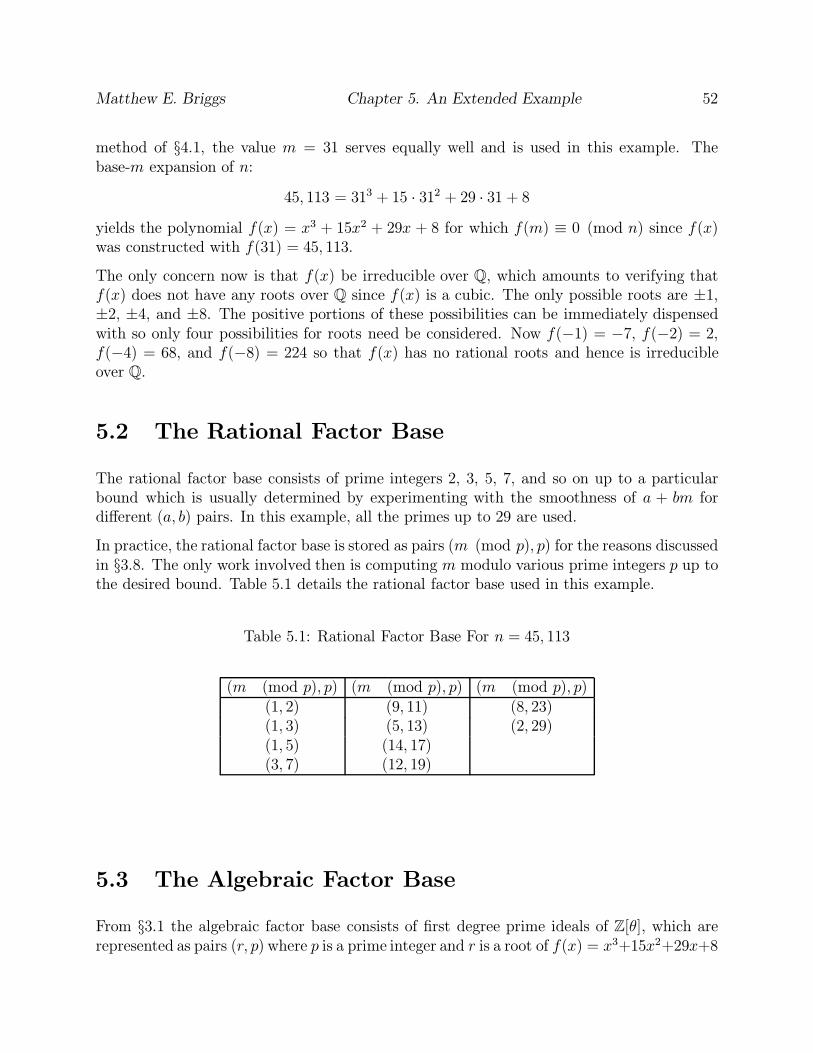
Matthew E. Briggs Chapter 5. An Extended Example 52
method of §4.1, the value m = 31 serves equally well and is used in this example. Thebase-m expansion of n:
45, 113 = 313 + 15 · 312 + 29 · 31 + 8
yields the polynomial f(x) = x3 + 15x2 + 29x + 8 for which f(m) ≡ 0 (mod n) since f(x)was constructed with f(31) = 45, 113.
The only concern now is that f(x) be irreducible over Q , which amounts to verifying thatf(x) does not have any roots over Q since f(x) is a cubic. The only possible roots are ±1,±2, ±4, and ±8. The positive portions of these possibilities can be immediately dispensedwith so only four possibilities for roots need be considered. Now f(−1) = −7, f(−2) = 2,f(−4) = 68, and f(−8) = 224 so that f(x) has no rational roots and hence is irreducibleover Q .
5.2 The Rational Factor Base
The rational factor base consists of prime integers 2, 3, 5, 7, and so on up to a particularbound which is usually determined by experimenting with the smoothness of a + bm fordifferent (a, b) pairs. In this example, all the primes up to 29 are used.
In practice, the rational factor base is stored as pairs (m (mod p), p) for the reasons discussedin §3.8. The only work involved then is computing m modulo various prime integers p up tothe desired bound. Table 5.1 details the rational factor base used in this example.
Table 5.1: Rational Factor Base For n = 45, 113
(m (mod p), p) (m (mod p), p) (m (mod p), p)(1, 2) (9, 11) (8, 23)(1, 3) (5, 13) (2, 29)(1, 5) (14, 17)(3, 7) (12, 19)
5.3 The Algebraic Factor Base
From §3.1 the algebraic factor base consists of first degree prime ideals of Z [θ], which arerepresented as pairs (r, p) where p is a prime integer and r is a root of f(x) = x3+15x2+29x+8

Matthew E. Briggs Chapter 5. An Extended Example 53
considered as a polynomial with coefficients in Z /pZ . Computing the algebraic factor basethen amounts to finding roots of f(x) modulo 2, 3, 5, 7 and so on.
Using the methods of §4.2 and the prime 67 as an example, start by computing the polynomialg(x) = gcd(f(x), x67−x) where g(x) serves to isolate the linear factors of f(x). In this case,g(x) ≡ f(x) (mod 67) so that f(x) consists of all linear factors and hence must have threeroots over Z /67Z .
Now g(0) ≡ 8 (mod 67) so that 0 is not a root of g(x). Since g(x) divides x67 − x =x(x33 + 1)(x33 − 1) it follows that g(x) must divide (x33 + 1)(x33 − 1) and in fact
g(x) ≡ gcd(x33 + 1, g(x)) · gcd(x33 − 1, g(x)) ≡ (x2 + 21x + 21) · (x+ 61) (mod 67).(5.1)
Hence, 6 ≡ −61 (mod 67) is a root of g(x) in Z /67Z and the pair (6, 67) represents a firstdegree prime ideal of Z [θ] that may be added to the algebraic factor base.
The same process can be used to determine the linear factors of g1(x) = x2 + 21x+ 21. Nowg1(−1) ≡ 1 (mod 67) so that −1 is not a root of g1(x) and hence g1(x − 1) must divide(x33 + 1)(x33 − 1) for the same reason g(x) does. However, gcd(x33 − 1, g1(x − 1)) ≡ 1(mod 67) so that g1(x− 1) can’t be immediately split into non-trivial factors as was done
with g(x) in (5.1).
Continuing on with g1(−2) ≡ 50 (mod 67) it is seen that −2 is not a root of g1(x) and henceg1(x− 2) must then divide (x33 + 1)(x33 − 1). This time luck prevails and
g1(x− 2) ≡ gcd(x33 + 1, g1(x− 2)) · gcd(x33 − 1, g1(x− 2))
≡ (x+ 21) · (x+ 63) (mod 67).
The latter yields 46 ≡ −21 (mod 67) and 4 ≡ −63 (mod 67) as roots of g1(x− 2), so that44 and 2 are roots of g1(x) over Z /67Z and hence the pairs (2, 67) and (44, 67) represent firstdegree prime ideals of Z [θ] which may be used in the algebraic factor base.
Root finding with primes other than 67 is performed in the exact same manner to determinethe rest of the algebraic factor base shown in Table 5.2.
5.4 The Quadratic Character Base
Since the quadratic character base of §3.2 is simply a small set of first degree prime ideals ofZ [θ] that don’t occur in the algebraic factor base, in practice one begins searching for rootsof f(x) modulo primes q with q strictly greater than the largest prime p occurring in a (r, p)pair in the algebraic factor base. The worked example of §5.3 serves as ample illustration ofhow the quadratic character base seen in Table 5.3 is computed.

Matthew E. Briggs Chapter 5. An Extended Example 54
Table 5.2: Algebraic Factor Base For n = 45, 113
(r, p) pair (r, p) pair (r, p) pair (r, p) pair(0, 2) (19, 41) (44, 67) (62, 89)(6, 7) (13, 43) (50, 73) (73, 89)
(13, 17) (1, 53) (23, 79) (28, 97)(11, 23) (46, 61) (47, 79) (87, 101)(26, 29) (2, 67) (73, 79) (47, 103)(18, 31) (6, 67) (28, 89)
Table 5.3: Quadratic Character Base For n = 45, 113
(r, p) pair (r, p) pair (r, p) pair(4, 107) (80, 107) (99, 109)(8, 107) (52, 109)
5.5 Sieving
For this example, the sieving interval is chosen such that −1000 < a < 1000 for b starting at1 and proceeding through 2, 3, 4, and so on until more than 39 (a, b) pairs are found witha+ bm and a+ bθ smooth. Finding more than 39 pairs will guarantee a linear dependenceamong the binary vectors associated with those pairs, which leads to perfect squares in Zand Z [θ] as explained in §4.3.
A straight forward implementation technique is to have two sieve arrays in memory, one fora + bm and the other for N(a + bθ), each with 2000 entries for all the possible a values fora fixed b. Sieving for smooth values of a+ bm proceeds exactly as in §3.5. For instance, thevalues of a for which a+bm is divisible by the prime 5 for b = 7 are of the form a = −7m+5kfor k ∈ Z such that −1000 < a < 1000. From Table 5.1 it is seen that m ≡ 1 (mod 5) andhence a is of the form a = −7 + 5k for k ∈ Z . The positions in the sieve array for a + bmcorresponding to an a value of −997, −992, . . . , −12, −7, −2, 3, 8, 13, . . . , 993, 998 thenhave ln(5) added to their value. This procedure is repeated for all the pairs of Table 5.1.A similar procedure is followed with the (r, p) pairs of Table 5.2 and the sieve array forN(a+ bθ). Each sieve array is then scanned for positions with positive value in accordancewith §3.6 and for such values a+ bm and N(a+ bθ) are trial divided to test for smoothness.The whole procedure is then repeated for the next value of b.
After enough sieving, 40 (a, b) pairs are found with a + bm and a + bθ smooth, as seen in

Matthew E. Briggs Chapter 5. An Extended Example 55
Table 5.4: (a, b) Pairs Found During Sieving
(a, b) pair (a, b) pair (a, b) pair (a, b) pair (a, b) pair (a, b) pair (a, b) pair(−73, 1) (−2, 1) (−1, 1) (2, 1) (3, 1) (4, 1) (8, 1)(13, 1) (14, 1) (15, 1) (32, 1) (56, 1) (61, 1) (104, 1)(116, 1) (−5, 2) (3, 2) (25, 2) (33, 2) (−8, 3) (2, 3)(17, 3) (19, 4) (48, 5) (54, 5) (313, 5) (−43, 6) (−8, 7)(11, 7) (38, 7) (44, 9) (4, 11) (119, 11) (856, 11) (536, 15)(5, 17) (5, 31) (9, 32) (−202, 43) (24, 55)
Table 5.4.
5.6 Forming the Matrix
To find the set U in Note 2.4.1, first a binary matrix B is constructed as in §4.3, where asingle column of the matrix corresponds to an (a, b) pair found in §5.5 with a+bm and a+bθsmooth. Since there are 10 primes in the rational factor base, 23 first degree prime idealsin the algebraic factor base, and 5 first degree prime ideals in the quadratic character base,each column of the matrix will have 39 entries, or 39 total rows for the matrix (one bit isadded for the sign of a+ bm).
To show explicitly how the matrix is formed, the column entry for the pair (−8, 3) foundin §5.5 will be calculated. The first entry is set to 0 since a + bm = −8 + 3 · 31 = 85 ispositive. The next 10 entries in this column vector are determined from the factorization ofa+ bm = 85 over the rational factor base:
85 = 20 · 30 · 51 · 70 · 110 · 130 · 171 · 190 · 230 · 290
where all the primes in the rational factor base have been shown for clarity. The columnvector for (−8, 3) then has 10 entries formed by taking the above 10 exponent vectors modulo2:
(0, 0, 1, 0, 0, 0, 1, 0, 0, 0)
Next, the norm of (−8, 3) is computed and factored over the primes occurring in first de-gree prime ideal pairs in the algebraic factor base. Recalling from (3.4) that N(a + bθ) =(−b)df(−a/b) it follows that the norm of an element a + bθ with d = 3 and f(x) =
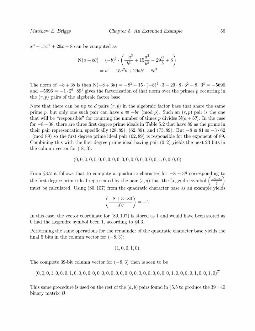
Matthew E. Briggs Chapter 5. An Extended Example 56
x3 + 15x2 + 29x+ 8 can be computed as
N(a+ bθ) = (−b)3 ·(−a3
b3+ 15
a2
b2− 29
a
b+ 8
)= a3 − 15a2b+ 29ab2 − 8b3.
The norm of −8 + 3θ is then N(−8 + 3θ) = −83 − 15 · (−8)2 · 3− 29 · 8 · 32 − 8 · 33 = −5696and −5696 = −1 · 26 · 891 gives the factorization of that norm over the primes p occurring inthe (r, p) pairs of the algebraic factor base.
Note that there can be up to d pairs (r, p) in the algebraic factor base that share the sameprime p, but only one such pair can have a ≡ −br (mod p). Such an (r, p) pair is the onethat will be “responsible” for counting the number of times p divides N(a+ bθ). In the casefor −8+3θ, there are three first degree prime ideals in Table 5.2 that have 89 as the prime intheir pair representation, specifically (28, 89), (62, 89), and (73, 89). But −8 ≡ 81 ≡ −3 · 62(mod 89) so the first degree prime ideal pair (62, 89) is responsible for the exponent of 89.
Combining this with the first degree prime ideal having pair (0, 2) yields the next 23 bits inthe column vector for (-8, 3):
(0, 0, 0, 0, 0, 0, 0, 0, 0, 0, 0, 0, 0, 0, 0, 0, 0, 0, 1, 0, 0, 0, 0)
From §3.2 it follows that to compute a quadratic character for −8 + 3θ corresponding to
the first degree prime ideal represented by the pair (s, q) that the Legendre symbol(−8+3sq
)must be calculated. Using (80, 107) from the quadratic character base as an example yields(
−8 + 3 · 80
107
)= −1.
In this case, the vector coordinate for (80, 107) is stored as 1 and would have been stored as0 had the Legendre symbol been 1, according to §4.3.
Performing the same operations for the remainder of the quadratic character base yields thefinal 5 bits in the column vector for (−8, 3):
(1, 0, 0, 1, 0).
The complete 39-bit column vector for (−8, 3) then is seen to be
(0, 0, 0, 1, 0, 0, 0, 1, 0, 0, 0, 0, 0, 0, 0, 0, 0, 0, 0, 0, 0, 0, 0, 0, 0, 0, 0, 0, 0, 1, 0, 0, 0, 0, 1, 0, 0, 1, 0)T
This same procedure is used on the rest of the (a, b) pairs found in §5.5 to produce the 39×40binary matrix B.
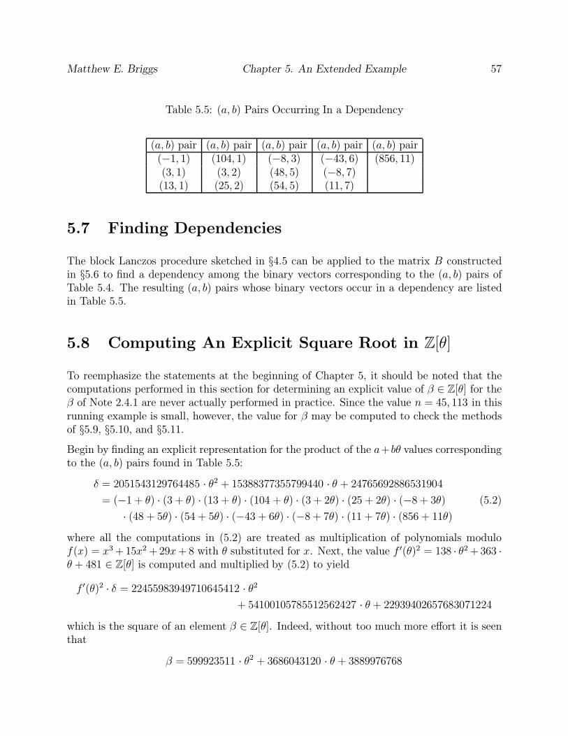
Matthew E. Briggs Chapter 5. An Extended Example 57
Table 5.5: (a, b) Pairs Occurring In a Dependency
(a, b) pair (a, b) pair (a, b) pair (a, b) pair (a, b) pair(−1, 1) (104, 1) (−8, 3) (−43, 6) (856, 11)(3, 1) (3, 2) (48, 5) (−8, 7)(13, 1) (25, 2) (54, 5) (11, 7)
5.7 Finding Dependencies
The block Lanczos procedure sketched in §4.5 can be applied to the matrix B constructedin §5.6 to find a dependency among the binary vectors corresponding to the (a, b) pairs ofTable 5.4. The resulting (a, b) pairs whose binary vectors occur in a dependency are listedin Table 5.5.
5.8 Computing An Explicit Square Root in Z [θ]
To reemphasize the statements at the beginning of Chapter 5, it should be noted that thecomputations performed in this section for determining an explicit value of β ∈ Z [θ] for theβ of Note 2.4.1 are never actually performed in practice. Since the value n = 45, 113 in thisrunning example is small, however, the value for β may be computed to check the methodsof §5.9, §5.10, and §5.11.
Begin by finding an explicit representation for the product of the a+bθ values correspondingto the (a, b) pairs found in Table 5.5:
δ = 2051543129764485 · θ2 + 15388377355799440 · θ + 24765692886531904
= (−1 + θ) · (3 + θ) · (13 + θ) · (104 + θ) · (3 + 2θ) · (25 + 2θ) · (−8 + 3θ)
· (48 + 5θ) · (54 + 5θ) · (−43 + 6θ) · (−8 + 7θ) · (11 + 7θ) · (856 + 11θ)
(5.2)
where all the computations in (5.2) are treated as multiplication of polynomials modulof(x) = x3 + 15x2 + 29x+ 8 with θ substituted for x. Next, the value f ′(θ)2 = 138 · θ2 + 363 ·θ + 481 ∈ Z [θ] is computed and multiplied by (5.2) to yield
f ′(θ)2 · δ = 22455983949710645412 · θ2
+ 54100105785512562427 · θ + 22939402657683071224
which is the square of an element β ∈ Z [θ]. Indeed, without too much more effort it is seenthat
β = 599923511 · θ2 + 3686043120 · θ + 3889976768

Matthew E. Briggs Chapter 5. An Extended Example 58
satisfies β2 = f ′(θ)2 · δ in Z [θ].
Applying the ring homomorphism φ : Z [θ]→ Z /45113Z of Proposition 2.4.1 to β gives
x = 43922 ≡ 694683807559 ≡599923511 · 312 + 3686043120 · 31 + 3889976768 ≡ φ(β) (mod 45331)
and it is this value x = 43, 922 that should result from the square root techniques of §5.9,§5.10, and §5.11.
5.9 Determining Applicable Finite Fields
The first stage in computing x = φ(β) (mod p) using the methods outlined in §4.6, §4.7,and §4.8 is to find a number of finite fields that are “compatible” with Q (θ), which boilsdown to finding prime integers p for which f(x) remains irreducible modulo p. First, f(x) =x3 + 15x2 + 29x + 8 will be tested for irreducibility modulo the prime p = 9929 using thetechniques of §4.9.
Begin by computing xp − x modulo f(x)
x9929− x ≡ 7449x2 + 4697x + 5984 (mod f(x))
and then taking the greatest common divisor with f(x) gives
gcd(7449x2 + 4697x + 5984, x3 + 15x2 + 29x+ 8) = 1
when considered modulo 9929. Thus, f(x) is irreducible over Z /9929Z by Theorem 4.9.5and the finite field F 99293 may be used in the methods of §4.6, §4.7, and §4.8.
As an example of a value for p for which f(x) does not turn out to be irreducible, if p = 9923then
x9923− x ≡ 7726x2 + 1477x + 7301 (mod f(x))
and the greatest common divisor turns out to be
gcd(7726x2 + 1477x + 7301, x3 + 15x2 + 29x + 8) = x− 847
modulo 9923. Hence 847 is a root of f(x) modulo 9923 and therefore f(x) is not irreducibleover Z /9923Z .
Table 5.6 lists the three primes pi for which the finite field F p3i
will be used in §5.10 and§5.11 for computing x in §5.8.

Matthew E. Briggs Chapter 5. An Extended Example 59
Table 5.6: Primes Determining Finite Fields F p3i
p0 p1 p2
9851 9907 9929
5.10 Square Roots in a Finite Field
The techniques of §4.8 will be illustrated for the prime p = 9929 and the finite field F p3,where the elements of the latter field may be represented as polynomials in θp where θp is aroot of f(x) in the splitting field of f(x) = x3 + 15x2 + 29x+ 8 over Z /pZ by Theorem 4.7.2.Denote F p3 by F p(θp) as well.
Begin by letting q = p3 so that q − 1 = 2r · s where r = 3 and s = 122356359011. The firsttask is to find a quadratic non-residue in F p(θp), which is very easy since exactly half theelements satisfy this property. A direct search immediately yields θp + 1 as a non-residue byTheorem 4.8.1 since
(θp + 1)99293−1
2 ≡ −1 (mod 9929).
From Theorem 4.8.3 it follows that the Sylow 2-subgroup S8 of F p(θp) can then be representedby the set
S8 ={
1, (θp + 1)s, (θp + 1)2s, (θp + 1)3s, . . . , (θp + 1)7s}.
Next, the element δ of §5.8 is computed in F p(θp) as
δp = 2027θ2p + 3891θp + 6659 ≡ f ′(θp)
2 · (−1 + θp) · (3 + θp) · (13 + θp)·(104 + θp) · (3 + 2θp) · (25 + 2θp) · (−8 + 3θp) · (48 + 5θp) ·(54 + 5θp) · (−43 + 6θp) · (−8 + 7θp) · (11 + 7θp) · (856 + 11θp)
The immediate goal is then to find an element ζ ∈ S8 with ζ2 ≡ δs. By direct computationin F p(θp) it is seen that δs ≡ 9928 (mod 9929) and from Table 5.7 it follows that ζ =(θp + 1)2s ≡ 2102 (mod 9929) is an element with the desired property.
If ω = δ(s+1)/2 then ν = ω · ζ−1 is a square root of δ since
ν2 ≡ ω2 · ζ−2 ≡ δs · δ · δ−s ≡ δ
since ζ was found such that ζ2 ≡ δs. Computing out ν explicitly involves computing themultiplicative inverse 7827 of ζ = 2102 modulo 9929 and then multiplying out
ν = ω · ζ−1 ≡ 7827 · δ s+12 ≡ 3402θ2
p + 1160θp + 3077.

Matthew E. Briggs Chapter 5. An Extended Example 60
Table 5.7: Members of S8 and Their Squares
i (θp + 1)is (θp + 1)2is i (θp + 1)is (θp + 1)2is
0 1 1 4 9928 11 1273 2102 5 8656 21022 2102 9928 6 7827 99283 4945 7827 7 4984 7827
Note that the other square root of δ is simply −ν in F p(θp), which is seen to be 6527θ2p +
8769θp + 6852
In the above description, the element ζ was found from the list of all its possible values inTable 5.7. The actual square root algorithm employed in §4.8 uses an iterative approach toavoid the explicit computation of all elements in S8. First, λ0 is initialized as λ0 = −1 ≡ δs(mod 9929) and ω0 is initialized as ω0 = 2124θ2
p + 5175θp + 4075 ≡ δ(s+1)/2. Finally, thevariable m is set to 1 since the order of λ0 in F ∗p3 is seen to be 2.
The iterative process begins by calculating λ1 and ω1 from λ0 and ω0. Letting ζ = (θp+1)s ≡1273 (mod 9929) then
λ1 ≡ λ0ζ2r−m ≡ −1 · 127323−1 ≡ −1 · 12734 ≡ 1 (mod 9929)
and
ω1 = ω0ζ2r−m−1 ≡ ω0 · 127323−1−1 ≡ ω0 · 12732 ≡ 6527θ2
p + 8769θp + 6852.
Since λ1 = 1 it follows that ω1 is a square root of δ, which is verified from the earliercalculation using Table 5.7.
5.11 Using the Chinese Remainder Theorem
From §5.8 it is known that the value of x is 694683807559 and hence x (mod 45113) = 43922.The goal of this section is to show that this value can be computed once square roots ofδ from §5.8 in the finite fields of Table 5.6 are known, as is done in §5.10. The relevantvalues from the computation of square roots in the finite fields of Table 5.6 are summarizedin Table 5.8.
For the sake of explanation, the value of z from §4.6 is computed as
z =2∑i=0
aixiPi = 7261482164111988.

Matthew E. Briggs Chapter 5. An Extended Example 61
Table 5.8: Square Roots of δ in Finite Fields
i = 0 i = 1 i = 2root 7462 · θ2
pi+ 5126 · θ2
pi+ 3402 · θ2
pi+
5791 · θpi + 4037 5072 · θpi + 3125 1160 · θpi + 3077xi 5694 4152 2002ai 7174 3691 8928pi 9851 9907 9929Pi 98366603 97810579 97593857
The value of P can also be computed as P = 9851 · 9907 · 9929 = 969009406153. Then it iseasily verified that z ≡ x (mod P ) and in fact 694683807559 = 7261482164111988 − 7493 ·969009406153 gives the value r = 7493 in x = z − rP . Note that these computations arenever carried out in practice and are done here only to verify the results of the remainingportions of the example. In the rest of this section it should be noted that all calculationstake place modulo n, which avoids the problems of unbounded integers when using directcomputations.
Begin by computing the value of r using
z
P=
2∑i=0
aixipi
=7174 · 5694
9851+
3691 · 4152
9907+
8928 · 2002
9929= 7493.72.
Rounding the last result yields r = 7493, which is indeed the correct value for r found bydirect calculation. In this computation it should be noted that neither x nor z needs to becalculated explicitly; only relatively small floating point numbers are required.
The value for x (mod n) can now be computed as
x (mod n) ≡2∑i=0
aixiPi (mod n) − rP (mod n)
≡ (a0x0p1p2) (mod n) + (a1x1p0p2) (mod n)
+ (a2x2p0p1) (mod n)− (rp0p1p2) (mod n)
≡ 7174 · 5694 · 9907 · 9929 (mod 45113)
+ 3691 · 4152 · 9851 · 9929 (mod 45113)
+ 8928 · 2002 · 9851 · 9907 (mod 45113)
− 7493 · 9851 · 9907 · 9929 (mod 45113)
≡ (41457 + 26833 + 42022 − 21277) (mod 45113)
≡ 43922 (mod 45113)
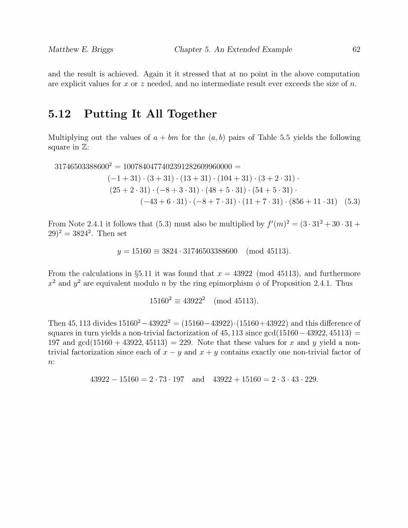
Matthew E. Briggs Chapter 5. An Extended Example 62
and the result is achieved. Again it it stressed that at no point in the above computationare explicit values for x or z needed, and no intermediate result ever exceeds the size of n.
5.12 Putting It All Together
Multiplying out the values of a + bm for the (a, b) pairs of Table 5.5 yields the followingsquare in Z :
317465033886002 = 1007840477402391282609960000 =
(−1 + 31) · (3 + 31) · (13 + 31) · (104 + 31) · (3 + 2 · 31) ·(25 + 2 · 31) · (−8 + 3 · 31) · (48 + 5 · 31) · (54 + 5 · 31) ·
(−43 + 6 · 31) · (−8 + 7 · 31) · (11 + 7 · 31) · (856 + 11 · 31) (5.3)
From Note 2.4.1 it follows that (5.3) must also be multiplied by f ′(m)2 = (3 · 312 + 30 · 31 +29)2 = 38242. Then set
y = 15160 ≡ 3824 · 31746503388600 (mod 45113).
From the calculations in §5.11 it was found that x = 43922 (mod 45113), and furthermorex2 and y2 are equivalent modulo n by the ring epimorphism φ of Proposition 2.4.1. Thus
151602 ≡ 439222 (mod 45113).
Then 45, 113 divides 151602−439222 = (15160−43922)·(15160+43922) and this difference ofsquares in turn yields a non-trivial factorization of 45, 113 since gcd(15160−43922, 45113) =197 and gcd(15160 + 43922, 45113) = 229. Note that these values for x and y yield a non-trivial factorization since each of x− y and x+ y contains exactly one non-trivial factor ofn:
43922 − 15160 = 2 · 73 · 197 and 43922 + 15160 = 2 · 3 · 43 · 229.
Chapter 6
Polynomial Selection and ParameterTuning
The first step of GNFS, selecting a polynomial, also happens to also be most important step.For any given integer n that is to be factored, there can literally be billions of choices for thepolynomial f(x) and the integer m with f(m) ≡ 0 (mod n). From real-world experimentswith the GNFS it has been seen that in many cases some polynomials are remarkably betterthan others, where a polynomial f(x) is considered “better” than another polynomial g(x) ifmore (a, b) pairs with a+ bm and 〈a+ bθ〉 smooth are found with f(x) than with g(x) usingthe same sieve interval, factor base sizes, and quadratic character base sizes. Although acrucial stage of the GNFS, polynomial selection still remains an ad-hoc and underdevelopedarea. Success relies upon some basic heuristic reasoning, lots of experimentation, and oftentimes just blind luck.
The goal here, then, is to explain how the experimentation phase of the GNFS proceeds,starting with an initial n to factor, proceeding on to trials of various candidate polynomials,and concluding with tuning the sieve for a particular selection of polynomial, factor base,and sieve interval.
6.1 Tweaking the Base-m Method
One begins polynomial selection by choosing an integer m close to n1/d such that
n = cd ·md + cd−1 ·md−1 + · · · + c1 ·m+ c0
and cd = 1. Then f(x) is defined to be f(x) = xd + cd−1xd−1 + · · · + c1x + c0 and byconstruction then f(m) = n ≡ 0 (mod n). If f(x) turns out to be reducible, then a non-trivial factorization of n is likely to be available immediately, in which case the processterminates successfully.
63

Matthew E. Briggs Chapter 6. Polynomial Selection and Parameter Tuning 64
One prominent strategy for producing “better” polynomials has been to reduce the sizes ofthe coefficients ci in f(x), with the idea being that the smaller these coefficients are, themore likely N(a+ bθ) is to be small. If N(a+ bθ) is relatively small it stands to reason thatit is more likely to factor over a small set of primes, and hence the more likely 〈a+ bθ〉 is tofactor over the algebraic factor base.
With this in mind, begin by noting that the base-m method produces an f(x) such that|ci| < m for 0 ≤ i < d. It turns out that this can be improved to |ci| < m/2, as follows. Forany ci > m/2 then m− ci < m/2. If 0 ≤ i < d− 1 then
(ci+1 + 1) ·mi+1 − (m− ci) ·mi = ci+1 ·mi+1 +mi+1 −mi+1 + ci ·mi = ci+1 ·mi+1 + cimi.
Hence, one can obtain an equivalent base-m expansion for n by replacing ci+1 with ci+1 + 1and ci with −(m− ci) for any ci > m/2. This expansion has the benefit that all coefficientsthen have absolute value less than m/2, if negative coefficients are allowed. Note i is chosenless than d− 1 so that the polynomial stays monic.
6.2 Using Polynomials of the Formf (x) + g(x)
The technique outlined in §6.1 of adjusting an existing polynomial f(x) with f(m) ≡ 0(mod n) can be expanded upon by adding another polynomial g(x) for which g(m) = 0.
Such polynomials are not too difficult to come up with, and in fact if
g(x) =d−1∑i=1
ci · (xi −mxi−1) (6.1)
then it is easily seen that g(m) = 0 since
g(m) =d−1∑i=1
ci · (mi −m ·mi−1) =d−1∑i=1
ci · (mi −mi) = 0.
To summarize, polynomial selection begins with an integer m ≈ n1/d and proceeds by ex-panding n base-m. The polynomial generated by this method can be further “tweaked”to insure that all coefficients have absolute value less than m/2. With or without this ad-justment, the polynomials of the base-m method can lead to other polynomials by addingpolynomials of the form shown in (6.1). Note polynomials of the form seen in (6.1) areproduced simply by choosing different values for c1, c2, . . . , cd−1.
6.3 Finding a Good Polynomial
Having chosen candidate polynomials for GNFS, the next step is to choose a few differentsizes for factor bases and sieve intervals, and then simply to sieve each polynomial using

Matthew E. Briggs Chapter 6. Polynomial Selection and Parameter Tuning 65
these different parameter choices. For the sake of brevity, the term “smooth” is applied hereto an (a, b) pair if that pair has a + bm and 〈a + bθ〉 smooth over their respective factorbases. The idea here is to find a polynomial that produces the most smooth (a+ b) pairs inthe shortest amount of time. For any given polynomial and factor base, the sieve interval isvaried and for each interval the number of smooth values found and the time it took to findthem is recorded. An estimate for the ratio of time taken to smooth (a, b) pairs can then bemade and compared with other ratios for the same polynomial and factor base. The intervalwith the smallest ratio is then selected and multiplied by an estimate for the total numberof pairs needed (rational primes + algebraic primes + quadratic characters will suffice) toestimate the shortest amount of time it will take to produce enough pairs, for the givenpolynomial and factor base. This latter statistic is recorded, and then the same procedurefor different factor bases with the same polynomial is performed. Once “enough” factor baseshave been examined, the factor base with the shortest time estimate for producing (a, b) pairsis chosen. This last figure represents the best performance for a particular polynomial, overa variety of factor bases and sieve intervals. The whole procedure can then be done againfor other polynomials, with the polynomial being selected for the GNFS being the one withthe shortest estimated time to produce enough (a, b) pairs.
6.4 Example Polynomial Selection
As an example of the different polynomial selection procedures and the aforementionedstrategy for selecting factor bases and sieve intervals, these techniques will be applied to thenumber
n = 556158012756522140970101270050308458769458529626977
where n is seen to be a 51 digit integer. Polynomials of degree d = 3 are generally used inthe GNFS for numbers of this size.
Begin by noting that
n1/3 ≈ 82236774153802891
so set m = 82236774153802891 and perform a base-m expansion on n to get
n = (82236774153802891)3 + 27709956990112403 ·(82236774153802891) + 45334438077235933
and hence f1(x) = x3 +27709956990112403x+45334438077235933 is a candidate polynomialfor n.
One can adjust the polynomial f1(x) by adding a polynomial g1(x) of the form g1(x) =c1 ·(x−m)+c2 ·(x2−m ·x), where c1 and c2 are usually chosen small to keep the coefficients
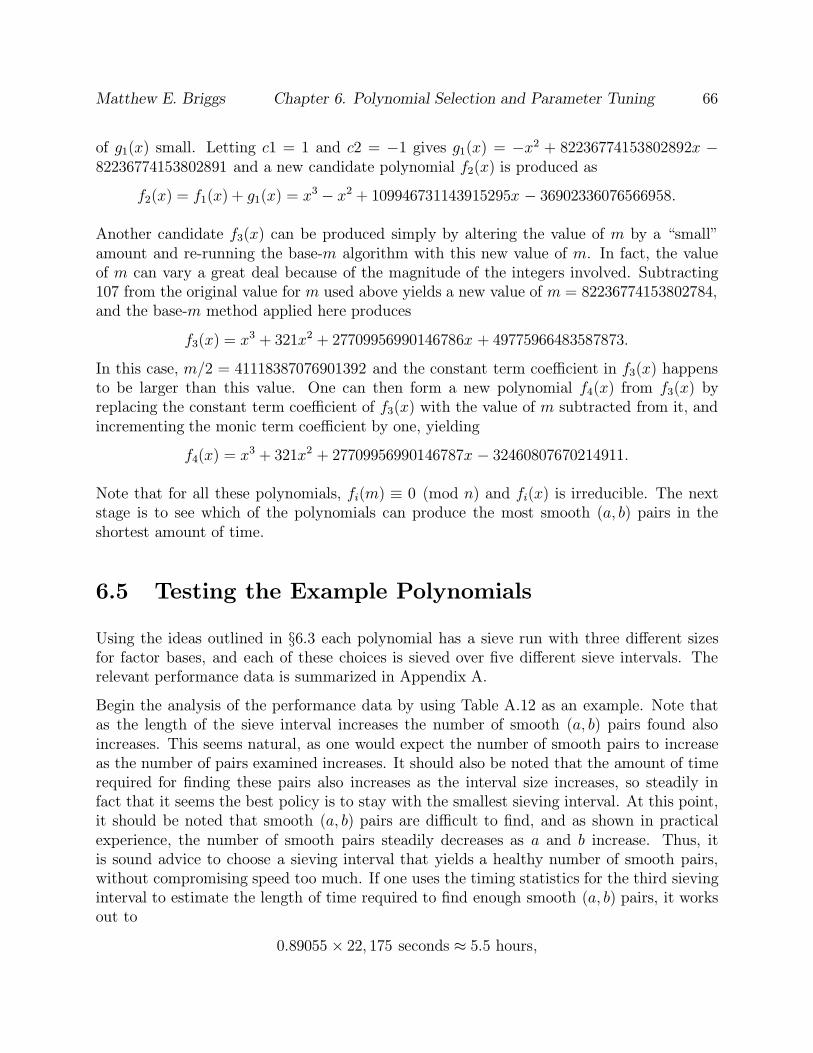
Matthew E. Briggs Chapter 6. Polynomial Selection and Parameter Tuning 66
of g1(x) small. Letting c1 = 1 and c2 = −1 gives g1(x) = −x2 + 82236774153802892x −82236774153802891 and a new candidate polynomial f2(x) is produced as
f2(x) = f1(x) + g1(x) = x3 − x2 + 109946731143915295x − 36902336076566958.
Another candidate f3(x) can be produced simply by altering the value of m by a “small”amount and re-running the base-m algorithm with this new value of m. In fact, the valueof m can vary a great deal because of the magnitude of the integers involved. Subtracting107 from the original value for m used above yields a new value of m = 82236774153802784,and the base-m method applied here produces
f3(x) = x3 + 321x2 + 27709956990146786x + 49775966483587873.
In this case, m/2 = 41118387076901392 and the constant term coefficient in f3(x) happensto be larger than this value. One can then form a new polynomial f4(x) from f3(x) byreplacing the constant term coefficient of f3(x) with the value of m subtracted from it, andincrementing the monic term coefficient by one, yielding
f4(x) = x3 + 321x2 + 27709956990146787x − 32460807670214911.
Note that for all these polynomials, fi(m) ≡ 0 (mod n) and fi(x) is irreducible. The nextstage is to see which of the polynomials can produce the most smooth (a, b) pairs in theshortest amount of time.
6.5 Testing the Example Polynomials
Using the ideas outlined in §6.3 each polynomial has a sieve run with three different sizesfor factor bases, and each of these choices is sieved over five different sieve intervals. Therelevant performance data is summarized in Appendix A.
Begin the analysis of the performance data by using Table A.12 as an example. Note thatas the length of the sieve interval increases the number of smooth (a, b) pairs found alsoincreases. This seems natural, as one would expect the number of smooth pairs to increaseas the number of pairs examined increases. It should also be noted that the amount of timerequired for finding these pairs also increases as the interval size increases, so steadily infact that it seems the best policy is to stay with the smallest sieving interval. At this point,it should be noted that smooth (a, b) pairs are difficult to find, and as shown in practicalexperience, the number of smooth pairs steadily decreases as a and b increase. Thus, itis sound advice to choose a sieving interval that yields a healthy number of smooth pairs,without compromising speed too much. If one uses the timing statistics for the third sievinginterval to estimate the length of time required to find enough smooth (a, b) pairs, it worksout to
0.89055 × 22, 175 seconds ≈ 5.5 hours,

Matthew E. Briggs Chapter 6. Polynomial Selection and Parameter Tuning 67
which is only 48 minutes more expensive than the shortest sieving interval. In practice, sincethe third sieving interval produced over one and a half times as many smooth (a, b) pairs asthe shortest sieving interval, it is probably the best one to use for this choice of polynomialand factor base.
After examining the data, the polynomial f4(x) stands out. Its performance ratio is betterthan all other polynomials for almost every choice of factor base sizes and sieve interval.
6.6 The Guessing Game
In should be noted how unpredictable the number of smooth (a, b) pairs produced is for anygiven selection of a polynomial, factor base, and sieving interval, even with this small dataset. For example, it appears as if the time required for finding smooth pairs increases asthe sieve interval increases for all the data examined, however that is not the case. There isactually a slight decrease in time when moving from the shortest interval to the next shortestinterval in Table A.1. However, that is not the case for the same polynomial and the sameintervals with larger factor bases, as seen in Table A.2 and Table A.3. Thus, a sieve intervalmay be extremely good for a polynomial with one factor base but produce terrible results forthe same polynomial with a different factor base. Another trend that seems evident is thatincreasing the sizes of the factor bases seems to decrease the overall estimated time for findingenough smooth (a, b) pairs. However as the factor base sizes increase this will not always betrue, since the larger primes in the larger factor bases occur in fewer a+ bm and N(a+ bθ)and hence are sieved with unnecessarily. Something of this sort is evidenced in Table A.4and Table A.5, where unlike any of the other polynomials, the estimated time increases fromthe smaller factor base to the larger. The inexplicable part comes from Table A.6, where theestimated time actually decreases from Table A.5.
To further debunk any kind of first glance intuition, one might initially guess that thepolynomial f1(x) would produce the most smooth pairs, since it has a coefficient of 0 for itsquadratic term. Indeed, it is the second-best performing polynomial, but as seen in the data,the best polynomial f4(x) also has the largest quadratic coefficient of all the polynomialstested. On the other hand, the worst-performing polynomial f3(x) has the same value asf4(x) for its quadratic term.
Even with a very small set of test cases, one can see that polynomial selection is still verymuch a “black” art that defies any sort of common sense intuition. There are billionsof candidate polynomials for large integers n and potentially a great deal of unexploitedstructure relating these polynomials and their probability of smoothness that needs to beinvestigated.

Matthew E. Briggs Chapter 6. Polynomial Selection and Parameter Tuning 68
6.7 An Alternate Strategy
A variation on the strategy detailed above cuts down dramatically on the amount of work thatgoes into screening candidate polynomials, with the end result being that more candidatepolynomials can be examined in a shorter amount of time. Upon examining the performancedata in Appendix A it is generally seen that when one polynomial performs better thananother for particular choices of factor base sizes and sieve interval, that polynomial willperform better than the other for all choices of factor base sizes and sieve intervals. Thebasic idea then is to judge all polynomials against one choice of factor base sizes and sieveinterval, stopping when a polynomial with dramatically better performance than any otheris found. That polynomial is then further optimized by running sieves with different factorbase sizes and sieve intervals as in §6.3. By using only a single selection of factor base sizesand sieve interval, the number of polynomials that can be examined in a given amount oftime is greatly increased.
More specifically, choose a polynomial and run multiple tests of factor base sizes and sieveintervals, as detailed in §6.3. When a mid-range parameter choice that balances the numberof smooth (a, b) pairs produced with the time required is found, that choice of factor basesizes and sieve interval will be be used as the test parameters for the remaining candidatepolynomials. All polynomials then run through a single test with the same factor base sizesand sieve interval, and the one with the least expected run time to find enough smooth pairsis kept. The original test with multiple factor base sizes and sieve intervals can then be runon the selected polynomial to further hone its performance. In fact, once the selection offactor base sizes and sieve interval are made, an automated tool can generate polynomials byvarying values for m, adjusting the coefficients of the base-m method, and substituting smallvalues for c1, c2, . . . , cd−1. The tool can further keep performance data while sieving withthe polynomials it generated. An end-user can then analyze the performance data for thevarious candidate polynomials when the tool is finished and choose the one that performsbest.
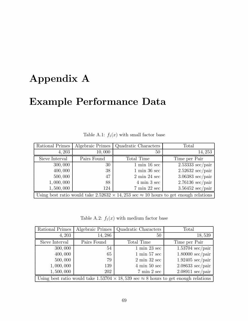
Appendix A
Example Performance Data
Table A.1: f1(x) with small factor base
Rational Primes Algebraic Primes Quadratic Characters Total4, 203 10, 000 50 14, 253
Sieve Interval Pairs Found Total Time Time per Pair300, 000 30 1 min 16 sec 2.53333 sec/pair400, 000 38 1 min 36 sec 2.52632 sec/pair500, 000 47 2 min 24 sec 3.06383 sec/pair
1, 000, 000 88 4 min 3 sec 2.76136 sec/pair1, 500, 000 124 7 min 22 sec 3.56452 sec/pair
Using best ratio would take 2.52632 × 14, 253 sec ≈ 10 hours to get enough relations
Table A.2: f1(x) with medium factor base
Rational Primes Algebraic Primes Quadratic Characters Total4, 203 14, 286 50 18, 539
Sieve Interval Pairs Found Total Time Time per Pair300, 000 54 1 min 23 sec 1.53704 sec/pair400, 000 65 1 min 57 sec 1.80000 sec/pair500, 000 79 2 min 32 sec 1.92405 sec/pair
1, 000, 000 139 4 min 50 sec 2.08633 sec/pair1, 500, 000 202 7 min 2 sec 2.08911 sec/pair
Using best ratio would take 1.53704 × 18, 539 sec ≈ 8 hours to get enough relations
69

Matthew E. Briggs Appendix A. Example Performance Data 70
Table A.3: f1(x) with large factor base
Rational Primes Algebraic Primes Quadratic Characters Total7, 837 14, 286 50 22, 173
Sieve Interval Pairs Found Total Time Time per Pair300, 000 102 1 min 28 sec 0.86275 sec/pair400, 000 127 1 min 50 sec 0.86614 sec/pair500, 000 153 2 min 38 sec 1.03268 sec/pair
1, 000, 000 249 5 min 10 sec 1.24498 sec/pair1, 500, 000 336 7 min 59 sec 1.42560 sec/pair
Using best ratio would take 0.86275 × 22, 173 sec ≈ 5.3 hours to get enough relations
Table A.4: f2(x) with small factor base
Rational Primes Algebraic Primes Quadratic Characters Total4, 203 10, 132 50 14, 385
Sieve Interval Pairs Found Total Time Time per Pair300, 000 45 1 min 26 sec 1.91111 sec/pair400, 000 54 2 min 1 sec 2.24074 sec/pair500, 000 65 2 min 32 sec 2.33846 sec/pair
1, 000, 000 106 5 min 11 sec 2.93396 sec/pair1, 500, 000 141 7 min 32 sec 3.20567 sec/pair
Using best ratio would take 1.91111 × 14, 385 sec ≈ 7.6 hours to get enough relations
Table A.5: f2(x) with medium factor base
Rational Primes Algebraic Primes Quadratic Characters Total4, 203 14, 296 52 18, 551
Sieve Interval Pairs Found Total Time Time per Pair300, 000 59 1 min 31 sec 1.54237 sec/pair400, 000 75 2 min 6 sec 1.68000 sec/pair500, 000 90 2 min 43 sec 1.81111 sec/pair
1, 000, 000 147 5 min 29 sec 2.23810 sec/pair1, 500, 000 198 7 min 53 sec 2.38889 sec/pair
Using best ratio would take 1.54237 × 18, 551 sec ≈ 7.9 hours to get enough relations
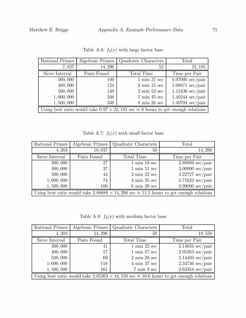
Matthew E. Briggs Appendix A. Example Performance Data 71
Table A.6: f2(x) with large factor base
Rational Primes Algebraic Primes Quadratic Characters Total7, 837 14, 296 52 22, 185
Sieve Interval Pairs Found Total Time Time per Pair300, 000 100 1 min 37 sec 0.97000 sec/pair400, 000 124 2 min 15 sec 1.08871 sec/pair500, 000 149 2 min 52 sec 1.15436 sec/pair
1, 000, 000 246 5 min 45 sec 1.40244 sec/pair1, 500, 000 338 8 min 26 sec 1.49704 sec/pair
Using best ratio would take 0.97× 22, 185 sec ≈ 6 hours to get enough relations
Table A.7: f3(x) with small factor base
Rational Primes Algebraic Primes Quadratic Characters Total4, 203 10, 037 50 14, 290
Sieve Interval Pairs Found Total Time Time per Pair300, 000 27 1 min 18 sec 2.88889 sec/pair400, 000 37 1 min 51 sec 3.00000 sec/pair500, 000 44 2 min 22 sec 3.22727 sec/pair
1, 000, 000 74 4 min 35 sec 3.71622 sec/pair1, 500, 000 100 6 min 39 sec 3.99000 sec/pair
Using best ratio would take 2.88889 × 14, 290 sec ≈ 11.5 hours to get enough relations
Table A.8: f3(x) with medium factor base
Rational Primes Algebraic Primes Quadratic Characters Total4, 203 14, 296 50 18, 550
Sieve Interval Pairs Found Total Time Time per Pair300, 000 41 1 min 22 sec 2.14634 sec/pair400, 000 57 1 min 57 sec 2.05263 sec/pair500, 000 69 2 min 28 sec 2.14493 sec/pair
1, 000, 000 118 4 min 37 sec 2.34746 sec/pair1, 500, 000 161 7 min 4 sec 2.63354 sec/pair
Using best ratio would take 2.05263 × 18, 550 sec ≈ 10.6 hours to get enough relations

Matthew E. Briggs Appendix A. Example Performance Data 72
Table A.9: f3(x) with large factor base
Rational Primes Algebraic Primes Quadratic Characters Total7, 837 14, 296 50 22, 184
Sieve Interval Pairs Found Total Time Time per Pair300, 000 87 1 min 30 sec 1.03448 sec/pair400, 000 115 2 min 7 sec 1.10435 sec/pair500, 000 136 2 min 40 sec 1.17647 sec/pair
1, 000, 000 220 5 min 23 sec 1.46818 sec/pair1, 500, 000 298 7 min 51 sec 1.58054 sec/pair
Using best ratio would take 1.03448 × 22, 184 sec ≈ 6.4 hours to get enough relations
Table A.10: f4(x) with small factor base
Rational Primes Algebraic Primes Quadratic Characters Total4, 203 10, 113 50 14, 366
Sieve Interval Pairs Found Total Time Time per Pair300, 000 50 1 min 29 sec 1.78000 sec/pair400, 000 64 2 min 4 sec 1.93750 sec/pair500, 000 74 2 min 38 sec 2.13514 sec/pair
1, 000, 000 109 5 min 18 sec 2.91743 sec/pair1, 500, 000 145 7 min 46 sec 3.21379 sec/pair
Using best ratio would take 1.78× 14, 366 sec ≈ 7.1 hours to get enough relations
Table A.11: f4(x) with medium factor base
Rational Primes Algebraic Primes Quadratic Characters Total4, 203 14, 288 50 18, 541
Sieve Interval Pairs Found Total Time Time per Pair300, 000 83 1 min 34 sec 1.13253 sec/pair400, 000 102 2 min 12 sec 1.29412 sec/pair500, 000 117 2 min 44 sec 1.40171 sec/pair
1, 000, 000 187 5 min 33 sec 1.78075 sec/pair1, 500, 000 241 8 min 7 sec 2.02075 sec/pair
Using best ratio would take 1.13253 × 18, 541 sec ≈ 5.8 hours to get enough relations

Matthew E. Briggs Appendix A. Example Performance Data 73
Table A.12: f4(x) with large factor base
Rational Primes Algebraic Primes Quadratic Characters Total7, 837 14, 288 50 22, 175
Sieve Interval Pairs Found Total Time Time per Pair300, 000 130 1 min 40 sec 0.76923 sec/pair400, 000 168 2 min 21 sec 0.83929 sec/pair500, 000 201 2 min 59 sec 0.89055 sec/pair
1, 000, 000 320 5 min 56 sec 1.11250 sec/pair1, 500, 000 428 8 min 43 sec 1.22196 sec/pair
Using best ratio would take 0.76923 × 22, 175 sec ≈ 4.7 hours to get enough relations

Bibliography
[1] Leonard M. Adleman, Factoring numbers using singular integers, Proceedings of the23rd Annual ACM Symposium on the Theory of Computing (STOC) (New Orleans),1991, pp. 64–71.
[2] David M. Bressoud, Factorization and primality testing, Undergraduate Texts in Math-ematics, Springer-Verlag, New York, 1989.
[3] John Brillhart, D.H. Lehmer, J.L. Selfridge, Bryant Tuckerman, and S.S. Wagstaff,Jr., Factorizations of bn ± 1, b = 2, 3, 5, 6, 7, 10, 11, 12 up to high powers, seconded., Contemporary Mathematics, vol. 22, American Mathematical Society, Providence,Rhode Island, 1988.
[4] J. Buchmann, J.Loho, and J.Zayer, An implementation of the general number fieldsieve, Advances in Cryptology (Proceedings of Crypto ’93) (Berlin), Lecture Notes inComputer Science, no. 773, Springer-Verlag, 1994, pp. 159–165.
[5] J.P. Buhler, H.W. Lenstra, Jr., and Carl Pomerance, Factoring integers with the numberfield sieve, In Lenstra and Lenstra [17], pp. 50–94.
[6] Henri Cohen, A course in computational algebraic number theory, Graduate Texts inMathematics, vol. 138, Springer-Verlag, Berlin, 1993.
[7] Jean-Marc Couveignes, Computing a square root for the number field sieve, In Lenstraand Lenstra [17], pp. 95–102.
[8] A.K. Lenstra Daniel J. Bernstein, A general number field sieve implementation, InLenstra and Lenstra [17], pp. 103–126.
[9] Bruce Dodson and Arjen K. Lenstra, NFS with four large primes: an explosive ex-periment, Advances in Cryptology (Crypto ’95) (Berlin), Lecture Notes in ComputerScience, no. 963, Springer-Verlag, 1995, pp. 372–385.
[10] David S. Dummit and Richard M. Foote, Abstract algebra, Prentice-Hall, EnglewoodCliffs, New Jersey, 1991.
74

Matthew E. Briggs Appendix A. Example Performance Data 75
[11] Stephen H. Friedberg, Arnold J. Insel, and Lawrence E. Spence, Linear algebra, seconded., Prentice-Hall, Englewood Cliffs, New Jersey, 1989.
[12] R.M. Huizing, An implementation of the number field sieve, Experimental Mathematics5 (1996), no. 3, 231–253.
[13] , A multiple polynomial general number field sieve, Algorithmic Number Theory(Berlin), Lecture Notes in Computer Science, vol. 1122, Springer-Verlag, 1996, pp. 99–114.
[14] Thomas W. Hungerford, Algebra, Graduate Texts in Mathematics, vol. 73, Springer-Verlag, New York, 1974.
[15] Donald E. Knuth, Seminumerical algorithms, second ed., The Art of Computer Pro-gramming, vol. 2, Addison-Wesley, Reading, Massachusetts, 1981.
[16] Ramanujachary Kumanduri, Number theory with computer applications, Prentice-Hall,Upper Saddle River, New Jersey, 1998.
[17] A.K. Lenstra and H.W. Lenstra, Jr. (eds.), The development of the number field sieve,Lecture Notes in Mathematics, vol. 1554, Berlin, Springer-Verlag, 1993.
[18] A.K. Lenstra, H.W. Lenstra, Jr., M.S. Manasse, and J.M. Pollard, The factorization ofthe ninth Fermat number, Mathematics of Computation 61 (1993), no. 203, 319–349.
[19] , The number field sieve, In Lenstra and Lenstra [17], pp. 11–42.
[20] A.K. Lenstra and M.S. Manasse, Factoring with two large primes, Mathematics of Com-putation 63 (1994), no. 208, 785–798.
[21] Rudolf Lidl and Harald Niederreiter, Introduction to finite fields and their applications,revised ed., Cambridge University Press, Cambridge, 1994.
[22] Peter L. Montgomery, Square roots of products of algebraic numbers, Proceedings ofSymposia in Applied Mathematics, Mathematics of Computation 1943–1993 (Vancou-ver) (Walter Gautschi, ed.), 1993.
[23] , A block Lanczos algorithm for finding dependencies over GF(2), Advances inCryptology – EUROCRYPT ’95 (Berlin) (L.C. Guillou and J.J. Quisquater, eds.), Lec-ture Notes in Computer Science, vol. 921, Springer-Verlag, 1995, pp. 106–120.
[24] Ivan Niven, Herbert S. Zuckerman, and Hugh L. Montgomery, An introduction to thetheory of numbers, fifth ed., John Wiley and Sons, New York, 1991.
[25] J.M. Pollard, The lattice sieve, In Lenstra and Lenstra [17], pp. 43–49.
[26] Carl Pomerance, A tale of two sieves, Notices of the American Mathematical Society43 (1996), no. 12, 1473–1485.

Matthew E. Briggs Appendix A. Example Performance Data 76
[27] Hans Riesel, Prime numbers and computer methods of factorization, second ed., Progressin Mathematics, vol. 126, Birkhauser, Boston, 1994.
[28] Kevin S. McCurley Roger A. Golliver, Arjen K. Lenstra, Lattice sieving and trial di-vision, Algorithmic Number Theory (Berlin) (L.M. Adleman and M.D. Huang, eds.),Lecture Notes in Computer Science, vol. 877, Springer-Verlag, 1994, pp. 18–27.
[29] Ian N. Stewart and David O. Tall, Algebraic number theory, second ed., Chapman andHall, London, July 1987.

Vita
Matthew Edward Briggs was born August 29, 1974 in Fairfax, Virginia to Tedford C. Briggsand Beverly D. Briggs. He is an only child who lived in the same house in Springfield,Virginia for 17 years before coming to Virginia Tech in the Fall of 1992. Matthew earned aBachelor of Science degree in Computer Science from Virginia Tech in the Spring of 1996,also graduating with a double major in Mathematics. Matthew immediately began Graduatestudy at Virginia Tech in the Summer of 1996 and continued on until the Spring of 1998when he received a Master of Science degree in Mathematics.
While pursuing his graduate degree at Virginia Tech, Matthew put his Computer Scienceskills to use working part-time at a local software company in the Virginia Tech CorporateResearch Center.
77