AN INTRODUCTION TO RELATIONAL DATABASES - …ce.sharif.edu/courses/84-85/2/ce384/resources/root/C. J... · · 2015-04-06AN INTRODUCTION TO RELATIONAL DATABASES 3.1 Introduction

59

CHAPTER3AN INTRODUCTION TO RELATIONAL DATABASES

3.1 Introduction3.2 An Informal Look at the Relational Model3.3 Relations and Relvars3.4 What Relations Mean3.5 Optimization3.6 The Catalog3.7 Base Relvars and Views3.8 Transactions3.9 The Suppliers-And-Parts Database3.10 Summary

ExercisesReferences and Bibliography

3.1 INTRODUCTION

As explained in Chapter 1, the emphasis in this book is heavily on relational systems. Inparticular, Part II covers the theoretical foundations of such systems—that is, the relationalmodel—in considerable depth. The purpose of the present chapter is to give a preliminary,intuitive, and very informal introduction to the material to be addressed in Part II (and tosome extent in subsequent parts too), in order to pave the way for a better understanding ofthose later parts of the book. Most of the topics mentioned will be discussed much moreformally, and in much more detail, in those later chapters.

Date Ch 03 Page 59 Saturday, May 3, 2003 5:45 PM

60 Part I / Preliminaries

3.2 AN INFORMAL LOOK AT THE RELATIONAL MODEL

We claimed in Chapter 1 that relational systems are based on a formal foundation,ortheory, called the relational model of data. The relational model is often described ashaving the following three aspects:

■ Structural aspect: The data in the database is perceived by the user as tables, andnothing but tables.

■ Integrity aspect: Those tables satisfy certain integrity constraints, to be discussedtoward the end of this section.

■ Manipulative aspect: The operators available to the user for manipulating thosetables—for example, for purposes of data retrieval—are operators that derive tablesfrom tables. Of those operators, three particularly important ones are restrict, project,and join.

A simple relational database, the departments-and-employees database, is shown inFig. 3.1. As you can see, that database is indeed “perceived as tables” (and the meaningsof those tables are intended to be self-evident).

Fig. 3.2 shows some sample restrict, project, and join operations against the databaseof Fig. 3.1. Here are (very loose!) definitions of those operations:

■ The restrict operation extracts specified rows from a table. Note: Restrict is some-times called select; we prefer restrict because the operator is not the same as theSELECT of SQL.

■ The project operation extracts specified columns from a table.

■ The join operation combines two tables into one on the basis of common values in acommon column.

Of the examples in the figure, the only one that seems to need any further explanationis the join example. Join requires the two tables to have a common column, which tablesDEPT and EMP do (they both have a column called DEPT#), and so they can be joined on

Fig. 3.1 The departments-and-employees database (sample values)

DEPT

EMP

DEPT# DNAME BUDGET

D1 Marketing 10MD2 Development 12MD3 Research 5M

EMP# ENAME DEPT# SALARY

E1 Lopez D1 40KE2 Cheng D1 42KE3 Finzi D2 30KE4 Saito D2 35K


Chapter 3 / An Introduction to Relational Databases 61

the basis of common values in that column. To be specific, a given row from table DEPTwill join to a given row in table EMP (to yield a row of the result table) if and only if thetwo rows in question have a common DEPT# value. For example, the DEPT and EMProws

(column names shown for explicitness) join together to produce the result row

because they have the same value, D1, in the common column. Note that the commonvalue appears once, not twice, in the result row. The overall result of the join contains allpossible rows that can be obtained in this manner, and no other rows. Observe in particularthat since no EMP row has a DEPT# value of D3 (i.e., no employee is currently assignedto that department), no row for D3 appears in the result, even though there is a row for D3in table DEPT.

Now, one point that Fig. 3.2 clearly shows is that the result of each of the three opera-tions is another table (in other words, the operators are indeed “operators that derivetables from tables,” as required). This is the closure property of relational systems, and itis very important. Basically, because the output of any operation is the same kind ofobject as the input—they are all tables— the output from one operation can become input

Fig. 3.2 Restrict, project, and join (examples)

DEPT# DNAME BUDGET EMP# ENAME DEPT# SALARY

D1 Marketing 10M E1 Lopez D1 40K

DEPT# DNAME BUDGET EMP# ENAME SALARY

D1 Marketing 10M E1 Lopez 40K

Restrict: Result:

DEPTs where BUDGET > 8M

DEPT# DNAME BUDGET

D1 Marketing 10MD2 Development 12M

Project: Result:

DEPTs over DEPT#, BUDGET

DEPT# BUDGET

D1 10MD2 12MD3 5M

Join:

DEPTs and EMPs over DEPT#

Result: DEPT# DNAME BUDGET EMP# ENAME SALARY

D1 Marketing 10M E1 Lopez 40KD1 Marketing 10M E2 Cheng 42KD2 Development 12M E3 Finzi 30KD2 Development 12M E4 Saito 35K



to another. Thus it is possible, for example, to take a projection of a join, a join of tworestrictions, a restriction of a projection, and so on. In other words, it is possible to writenested relational expressions—that is, relational expressions in which the operands them-selves are represented by relational expressions, not necessarily just by simple tablenames. This fact in turn has numerous important consequences, as we will see later, bothin this chapter and in many subsequent ones.

By the way, when we say that the output from each operation is another table, it isimportant to understand that we are talking from a conceptual point of view. We do notmean to imply that the system actually has to materialize the result of every individualoperation in its entirety.1 For example, suppose we are trying to compute a restriction of ajoin. Then, as soon as a given row of the join is formed, the system can immediately testthat row against the specified restriction condition to see whether it belongs in the finalresult, and immediately discard it if not. In other words, the intermediate result that is theoutput from the join might never exist as a fully materialized table in its own right at all.As a general rule, in fact, the system tries very hard not to materialize intermediate resultsin their entirety, for obvious performance reasons. Note: If intermediate results are fullymaterialized, the overall expression evaluation strategy is called (unsurprisingly) materi-alized evaluation; if intermediate results are passed piecemeal to subsequent operations,it is called pipelined evaluation.

Another point that Fig. 3.2 also clearly illustrates is that the operations are all set-at-a-time, not row-at-a-time; that is, the operands and results are whole tables, not just singlerows, and tables contain sets of rows. (A table containing a set of just one row is legal, ofcourse; as is an empty table, i.e., one containing no rows at all.) For example, the join inFig. 3.2 operates on two tables of three and four rows respectively, and returns a resulttable of four rows. By contrast, the operations in nonrelational systems are typically at therow- or record-at-a-time level; thus, this set processing capability is a major distinguish-ing characteristic of relational systems (see further discussion in Section 3.5).

Let us return to Fig. 3.1 for a moment. There are a couple of additional points to bemade in connection with the sample database of that figure:

■ First, note that relational systems require only that the database be perceived by theuser as tables. Tables are the logical structure in a relational system, not the physicalstructure. At the physical level, in fact, the system is free to store the data any way itlikes—using sequential files, indexing, hashing, pointer chains, compression, and soon—provided only that it can map that stored representation to tables at the logicallevel. Another way of saying the same thing is that tables represent an abstraction ofthe way the data is physically stored—an abstraction in which numerous storage-level details (such as stored record placement, stored record sequence, stored datavalue representations, stored record prefixes, stored access structures such as indexes,and so forth) are all hidden from the user.

Incidentally, the term logical structure in the foregoing paragraph is intended toencompass both the conceptual and external levels, in ANSI/SPARC terms. The pointis that—as explained in Chapter 2—the conceptual and external levels in a relational

1. In other words, to repeat from Chapter 1, the relational model is indeed a model—it has nothing to sayabout implementation.



system will both be relational, but the internal level will not be. In fact, relationaltheory as such has nothing to say about the internal level at all; it is, to repeat, con-cerned with how the database looks to the user.2 The only requirement is that, torepeat, whatever physical structure is chosen at the internal level must fully supportthe required logical structure.

■ Second, relational databases abide by a very nice principle, called The InformationPrinciple: The entire information content of the database is represented in one andonly one way—namely, as explicit values in column positions in rows in tables. Thismethod of representation is the only method available (at the logical level, that is) in arelational system. In particular, there are no pointers connecting one table toanother. In Fig. 3.1, for example, there is a connection between the D1 row of tableDEPT and the E1 row of table EMP, because employee E1 works in department D1;but that connection is represented, not by a pointer, but by the appearance of the valueD1 in the DEPT# position of the EMP row for E1. In nonrelational systems such asIMS or IDMS, by contrast, such information is typically represented—as mentionedin Chapter 1—by some kind of pointer that is explicitly visible to the user.

Note: We will explain in Chapter 26 just why allowing such user-visible pointerswould constitute a violation of The Information Principle. Also, when we say there areno pointers in a relational database, we do not mean there cannot be pointers at thephysical level—on the contrary, there certainly can, and indeed there almost certainlywill. But, to repeat, all such physical storage details are concealed from the user in arelational system.

So much for the structural and manipulative aspects of the relational model; now weturn to the integrity aspect. Consider the departments-and-employees database of Fig. 3.1once again. In practice, that database might be required to satisfy any number of integrityconstraints—for example, employee salaries might have to be in the range 25K to 95K(say), department budgets might have to be in the range 1M to 15M (say), and so on. Cer-tain of those constraints are of such major pragmatic importance, however, that they enjoysome special nomenclature. To be specific:

1. Each row in table DEPT must include a unique DEPT# value; likewise, each row intable EMP must include a unique EMP# value. We say, loosely, that columns DEPT#in table DEPT and EMP# in table EMP are the primary keys for their respectivetables. (Recall from Chapter 1 that we indicate primary keys in our figures by doubleunderlining.)

Each DEPT# value in table EMP must exist as a DEPT# value in table DEPT, toreflect the fact that every employee must be assigned to an existing department. Wesay, loosely, that column DEPT# in table EMP is a foreign key, referencing the pri-mary key of table DEPT.

2. It is an unfortunate fact that most of today’s SQL products do not support this aspect of the theoryproperly. To be more specific, they typically support only rather restrictive conceptual/internal mappings;typically, in fact, they map one logical table directly to one stored file. This is one reason why (as noted inChapter 1) those products do not provide as much data independence as relational technology is theoreti-cally capable of. See Appendix A for further discussion.



A More Formal Definition

We close this section with a somewhat more formal definition of the relational model, forpurposes of subsequent reference (despite the fact that the definition is quite abstract andwill not make much sense at this stage). Briefly, the relational model consists of the fol-lowing five components:

1. An open-ended collection of scalar types (including in particular the type boolean ortruth value)

2. A relation type generator and an intended interpretation for relations of types gen-erated thereby

3. Facilities for defining relation variables of such generated relation types

4. A relational assignment operation for assigning relation values to such relationvariables

5. An open-ended collection of generic relational operators (“the relational algebra”)for deriving relation values from other relation values

As you can see, the relational model is very much more than just “tables plus restrict,project, and join,” though it is often characterized in such a manner informally.

By the way, you might be surprised to see no explicit mention of integrity constraintsin the foregoing definition. The fact is, however, such constraints represent just one appli-cation of the relational operators (albeit a very important one); that is, such constraints areformulated in terms of those operators, as we will see in Chapter 9.

3.3 RELATIONS AND RELVARS

If it is true that a relational database is basically just a database in which the data is per-ceived as tables—and of course it is true—then a good question to ask is: Why exactly dowe call such a database relational? The answer is simple (in fact, we mentioned it in Chap-ter 1): Relation is just a mathematical term for a table—to be precise, a table of a specifickind (details to be pinned down in Chapter 6). Thus, for example, we can say that thedepartments-and-employees database of Fig. 3.1 contains two relations.

Now, in informal contexts it is usual to treat the terms relation and table as if they weresynonymous; in fact, the term table is used much more often than the term relation in prac-tice. But it is worth taking a moment to understand why the term relation was introduced inthe first place. Briefly:

■ As we have seen, relational systems are based on the relational model. The relationalmodel in turn is an abstract theory of data that is based on certain aspects of mathe-matics (mainly set theory and predicate logic).

■ The principles of the relational model were originally laid down in 1969–70 by E. F.Codd, at that time a researcher in IBM. It was late in 1968 that Codd, a mathemati-cian by training, first realized that the discipline of mathematics could be used toinject some solid principles and rigor into a field (database management) that prior to



that time was all too deficient in any such qualities. Codd’s ideas were first widelydisseminated in a now classic paper, “A Relational Model of Data for Large SharedData Banks” (reference [6.1] in Chapter 6).

■ Since that time, those ideas—by now almost universally accepted—have had a wide-ranging influence on just about every aspect of database technology, and indeed onother fields as well, such as the fields of artificial intelligence, natural language pro-cessing, and hardware design.

Now, the relational model as originally formulated by Codd very deliberately madeuse of certain terms, such as the term relation itself, that were not familiar in IT circles atthat time (even though the concepts in some cases were). The trouble was, many of themore familiar terms were very fuzzy—they lacked the precision necessary to a formal the-ory of the kind that Codd was proposing. For example, consider the term record. At differ-ent times and in different contexts, that single term can mean either a record occurrence ora record type; a logical record or a physical record; a stored record or a virtual record; andperhaps other things besides. The relational model therefore does not use the term recordat all—instead, it uses the term tuple (rhymes with couple), to which it gives a very pre-cise definition. We will discuss that definition in detail in Chapter 6; for present purposes,it is sufficient to say that the term tuple corresponds approximately to the notion of a row(just as the term relation corresponds approximately to the notion of a table).

In the same kind of way, the relational model does not use the term field; instead, ituses the term attribute, which for present purposes we can say corresponds approximatelyto the notion of a column in a table.

When we move on to study the more formal aspects of relational systems in Part II,we will make use of the formal terminology, but in this chapter we are not trying to be soformal (for the most part, at any rate), and we will mostly stick to terms such as row andcolumn that are reasonably familiar. However, one formal term we will start using a lotfrom this point forward is the term relation itself.

We return to the departments-and-employees database of Fig. 3.1 to make anotherimportant point. The fact is, DEPT and EMP in that database are really relation variables:variables, that is, whose values are relation values (different relation values at differenttimes). For example, suppose EMP currently has the value—the relation value, that is—shown in Fig. 3.1, and suppose we delete the row for Saito (employee number E4):

DELETE EMP WHERE EMP# = EMP# ('E4') ;

The result is shown in Fig. 3.3.

Fig. 3.3 Relation variable EMP after deleting E4 row

EMP EMP# ENAME DEPT# SALARY

E1 Lopez D1 40KE2 Cheng D1 42KE3 Finzi D2 30K



Conceptually, what has happened here is that the old relation value of EMP has beenreplaced en bloc by an entirely new relation value. Of course, the old value (with four rows)and the new one (with three) are very similar, but conceptually they are different values.Indeed, the delete operation in question is basically just shorthand for a certain relationalassignment operation that might look like this:

EMP := EMP WHERE NOT ( EMP# = EMP# ('E4') ) ;

As in all assignments, what is happening here, conceptually, is that (a) the expression onthe right side is evaluated, and then (b) the result of that evaluation is assigned to the vari-able on the left side (naturally that left side must identify a variable specifically). Asalready stated, the net effect is thus to replace the “old” EMP value by a “new” one. (As anaside, we remark that we have now seen our first examples of the use of the Tutorial D lan-guage—both the original DELETE and the equivalent assignment were expressed in thatlanguage.)

In analogous fashion, relational INSERT and UPDATE operations are also basicallyshorthand for certain relational assignments. See Chapter 6 for further details.

Now, it is an unfortunate fact that much of the literature uses the term relation whenwhat it really means is a relation variable (as well as when it means a relation per se—that is, a relation value). Historically, however, this practice has certainly led to some con-fusion. Throughout this book, therefore, we will distinguish very carefully between rela-tion variables and relations per se; following reference [3.3], in fact, we will use the termrelvar as a convenient shorthand for relation variable, and we will take care to phrase ourremarks in terms of relvars, not relations, when it really is relvars that we mean.3 Pleasenote, therefore, that from this point forward we take the unqualified term relation to meana relation value specifically (just as we take, e.g., the unqualified term integer to mean aninteger value specifically), though we will also use the qualified term relation value onoccasion, for emphasis.

Before going any further, we should warn you that the term relvar is not in commonusage—but it should be! We really do feel it is important to be clear about the distinctionbetween relations per se and relation variables. (We freely admit that earlier editions ofthis book failed in this respect, but then so did the rest of the literature. What is more,most of it still does.) Note in particular that, by definition, update operations and integrityconstraints—see Chapters 6 and 9, respectively—both apply specifically to relvars, notrelations.

3.4 WHAT RELATIONS MEAN

In Chapter 1, we mentioned the fact that columns in relations have associated data types(types for short, also known as domains). And at the end of Section 3.2, we said that therelational model includes “an open-ended set of . . . types.” Note carefully that the fact thatthe set is open-ended implies among other things that users will be able to define their

3. The distinction between relation values and relation variables is actually a special case of the distinc-tion between values and variables in general. We will examine this latter distinction in depth in Chapter 5.



own types (as well as being able to make use of system-defined or built-in types, ofcourse). For example, we might have user-defined types as follows (Tutorial D syntaxagain; the ellipses “. . .” denote portions of the definitions that are not germane to thepresent discussion):

TYPE EMP# ... ;TYPE NAME ... ;TYPE DEPT# ... ;TYPE MONEY ... ;

Type EMP#, for example, can be regarded (among other things) as the set of all possibleemployee numbers; type NAME as the set of all possible names; and so on.

Now consider Fig. 3.4, which is basically the EMP portion of Fig. 3.1 expanded toshow the column data types. As the figure indicates, every relation—to be more precise,every relation value—has two parts, a set of column-name:type-name pairs (the heading)together with a set of rows that conform to that heading (the body). Note: In practice weoften ignore the type-name components of the heading, as indeed we have done in all ofour examples prior to this point, but you should understand that, conceptually, they arealways there.

Now, there is a very important (though perhaps unusual) way of thinking about rela-tions, and that is as follows:

1. Given a relation r, the heading of r denotes a certain predicate (where a predicate isjust a truth-valued function that, like all functions, takes a set of parameters).

2. As mentioned briefly in Chapter 1, each row in the body of r denotes a certain trueproposition, obtained from the predicate by substituting certain argument values ofthe appropriate type for the parameters of the predicate (“instantiating the predi-cate”).

In the case of Fig. 3.4, for example, the predicate looks something like this:

Employee EMP# is named ENAME, works in department DEPT#, and earns salarySALARY

(the parameters are EMP#, ENAME, DEPT#, and SALARY, corresponding of course tothe four EMP columns). And the corresponding true propositions are:

Employee E1 is named Lopez, works in department D1, and earns salary 40K

(obtained by substituting the EMP# value E1, the NAME value Lopez, the DEPT# valueD1, and the MONEY value 40K for the appropriate parameters);

Fig. 3.4 Sample EMP relation value, showing column types

EMP# : EMP# ENAME : NAME DEPT# : DEPT# SALARY : MONEY




Employee E2 is named Cheng, works in department D1, and earns salary 42K

(obtained by substituting the EMP# value E2, the NAME value Cheng, the DEPT# valueD1, and the MONEY value 42K for the appropriate parameters); and so on. In a nutshell,therefore:

■ Types are (sets of) things we can talk about. ■ Relations are (sets of) things we say about the things we can talk about.

(There is a nice analogy here that might help you appreciate and remember these importantpoints: Types are to relations as nouns are to sentences.) Thus, in the example, the thingswe can talk about are employee numbers, names, department numbers, and money values,and the things we say are true utterances of the form “The employee with the specifiedemployee number has the specified name, works in the specified department, and earns thespecified salary.”

It follows from all of the foregoing that:

1. Types and relations are both necessary (without types, we have nothing to talk about;without relations, we cannot say anything).

2. Types and relations are sufficient, as well as necessary—i.e., we do not need anythingelse, logically speaking.

3. Types and relations are not the same thing. It is an unfortunate fact that certain com-mercial products—not relational ones, by definition!—are confused over this verypoint. We will discuss this confusion in Chapter 26 (Section 26.2).

By the way, it is important to understand that every relation has an associated predi-cate, including relations that are derived from others by means of operators such as join.For example, the DEPT relation of Fig. 3.1 and the three result relations of Fig. 3.2 havepredicates as follows:

■ DEPT: Department DEPT# is named DNAME and has budget BUDGET■ Restriction of DEPT where BUDGET > 8M: Department DEPT# is named DNAME

and has budget BUDGET, which is greater than eight million dollars■ Projection of DEPT over DEPT# and BUDGET: Department DEPT# has some name

and has budget BUDGET■ Join of DEPT and EMP over DEPT#: Department DEPT# is named DNAME and has

budget BUDGET and employee EMP# is named ENAME, works in departmentDEPT#, and earns salary SALARY (note that this predicate has six parameters, notseven—the two references to DEPT# denote the same parameter)

Finally, we observe that relvars have predicates too: namely, the predicate that iscommon to all of the relations that are possible values of the relvar in question. For exam-ple, the predicate for relvar EMP is:

Employee EMP# is named ENAME, works in department DEPT#, and earns salarySALARY



3.5 OPTIMIZATION

As explained in Section 3.2, the relational operators (restrict, project, join, and so on) areall set-level. As a consequence, relational languages are often said to be nonprocedural,on the grounds that users specify what, not how—that is, they say what they want, withoutspecifying a procedure for getting it. The process of “navigating” around the stored data inorder to satisfy user requests is performed automatically by the system, not manually bythe user. For this reason, relational systems are sometimes said to perform automatic nav-igation. In nonrelational systems, by contrast, navigation is generally the responsibility ofthe user. A striking illustration of the benefits of automatic navigation is shown in Fig. 3.5,which contrasts a certain SQL INSERT statement with the “manual navigation” code theuser might have to write to achieve an equivalent effect in a nonrelational system (actuallya CODASYL network system; the example is taken from the chapter on network databasesin reference [1.5]). Note: The database is the well-known suppliers-and-parts database.See Section 3.9 for further explanation.

INSERT INTO SP ( S#, P#, QTY ) VALUES ( 'S4', 'P3', 1000 ) ;

MOVE 'S4' TO S# IN SFIND CALC SACCEPT S-SP-ADDR FROM S-SP CURRENCYFIND LAST SP WITHIN S-SPwhile SP found PERFORM ACCEPT S-SP-ADDR FROM S-SP CURRENCY FIND OWNER WITHIN P-SP GET P IF P# IN P < 'P3' leave loop END-IF FIND PRIOR SP WITHIN S-SPEND-PERFORMMOVE 'P3' TO P# IN PFIND CALC PACCEPT P-SP-ADDR FROM P-SP CURRENCYFIND LAST SP WITHIN P-SP while SP found PERFORM ACCEPT P-SP-ADDR FROM P-SP CURRENCY FIND OWNER WITHIN S-SP GET S IF S# IN S < 'S4' leave loop END-IF FIND PRIOR SP WITHIN P-SP END-PERFORMMOVE 1000 TO QTY IN SPFIND DB-KEY IS S-SP-ADDRFIND DB-KEY IS P-SP-ADDR STORE SP CONNECT SP TO S-SPCONNECT SP TO P-SP

Fig. 3.5 Automatic vs. manual navigation



Despite the remarks of the previous paragraph, it has to be said that nonprocedural isnot a very satisfactory term, common though it is, because procedurality and nonproce-durality are not absolutes. The best that can be said is that some language A is either moreor less procedural than some other language B. Perhaps a better way of putting matterswould be to say that relational languages are at a higher level of abstraction than nonrela-tional languages (as Fig. 3.5 suggests). Fundamentally, it is this raising of the level ofabstraction that is responsible for the increased productivity that relational systems canprovide.

Deciding just how to perform the automatic navigation referred to above is the respon-sibility of a very important DBMS component called the optimizer (we mentioned thiscomponent briefly in Chapter 2). In other words, for each access request from the user, it isthe job of the optimizer to choose an efficient way to implement that request. By way of anexample, let us suppose the user issues the following query (Tutorial D once again):

( EMP WHERE EMP# = EMP# ('E4') ) { SALARY }

Explanation: The expression inside the outer parentheses (“EMP WHERE . . .”)denotes a restriction of the current value of relvar EMP to just the row for employee E4.The column name in braces ("SALARY") then causes the result of that restriction to beprojected over the SALARY column. The result of that projection is a single-column,single-row relation that contains employee E4’s salary. (Incidentally, note that we areimplicitly making use of the relational closure property in this example—we have writtena nested relational expression, in which the input to the projection is the output from therestriction.)

Now, even in this very simple example, there are probably at least two ways of per-forming the necessary data access:

1. By doing a physical sequential scan of (the stored version of) relvar EMP until therequired data is found

2. If there is an index on (the stored version of) the EMP# column—which in practicethere probably will be, because EMP# values are supposed to be unique, and manysystems in fact require an index in order to enforce uniqueness—then by using thatindex to go directly to the required data

The optimizer will choose which of these two strategies to adopt. More generally,given any particular request, the optimizer will make its choice of strategy for implement-ing that request on the basis of considerations such as the following:

■ Which relvars are referenced in the request ■ How big those relvars currently are ■ What indexes exist ■ How selective those indexes are ■ How the data is physically clustered on the disk ■ What relational operations are involved



and so on. To repeat, therefore: Users specify only what data they want, not how to get tothat data; the access strategy for getting to that data is chosen by the optimizer (“automaticnavigation”). Users and user programs are thus independent of such access strategies,which is of course essential if data independence is to be achieved.

We will have a lot more to say about the optimizer in Chapter 18.

3.6 THE CATALOG

As explained in Chapter 2, the DBMS must provide a catalog or dictionary function. Thecatalog is the place where—among other things—all of the various schemas (external,conceptual, internal) and all of the corresponding mappings (external/conceptual, concep-tual/internal, external/external) are kept. In other words, the catalog contains detailedinformation, sometimes called descriptor information or metadata, regarding the variousobjects that are of interest to the system itself. Examples of such objects are relvars,indexes, users, integrity constraints, security constraints, and so on. Descriptor informa-tion is essential if the system is to do its job properly. For example, the optimizer uses cat-alog information about indexes and other auxiliary structures, as well as much otherinformation, to help it decide how to implement user requests (see Chapter 18). Likewise,the authorization subsystem uses catalog information about users and security constraintsto grant or deny such requests in the first place (see Chapter 17).

Now, one of the nice features of relational systems is that, in such a system, the cata-log itself consists of relvars (more precisely, system relvars, so called to distinguish themfrom ordinary user ones). As a result, users can interrogate the catalog in exactly the sameway they interrogate their own data. For example, the catalog in an SQL system mightinclude two system relvars called TABLE and COLUMN, the purpose of which is todescribe the tables (or relvars) in the database and the columns in those tables. For thedepartments-and-employees database of Fig. 3.1, the TABLE and COLUMN relvarsmight look in outline as shown in Fig. 3.6.4

Note: As mentioned in Chapter 2, the catalog should normally be self-describing—thatis, it should include entries describing the catalog relvars themselves (see Exercise 3.3).

Now suppose some user of the departments-and-employees database wants to knowexactly what columns relvar DEPT contains (obviously we are assuming that for some rea-son the user does not already have this information). Then the expression

( COLUMN WHERE TABNAME = 'DEPT' ) { COLNAME }

does the job. Here is another example: “Which relvars include a column called EMP#?”

( COLUMN WHERE COLNAME = 'EMP#' ) { TABNAME }

4. Note that the presence of column ROWCOUNT in Fig. 3.6 suggests that INSERT and DELETE opera-tions on the database will cause an update to the catalog as a side effect. In practice, ROWCOUNT mightbe updated only on request (e.g., when some utility is run), meaning that values of that column might notalways be current.



Exercise: What does the following do?

( ( TABLE JOIN COLUMN ) WHERE COLCOUNT < 5 ) { TABNAME, COLNAME }

3.7 BASE RELVARS AND VIEWS

We have seen that, starting with a set of relvars such as DEPT and EMP, together with aset of relation values for those relvars, relational expressions allow us to obtain furtherrelation values from those given ones. It is time to introduce a little more terminology. Theoriginal (given) relvars are called base relvars, and their values are called base relations;a relation that is not a base relation but can be obtained from the base relations by meansof some relational expression is called a derived, or derivable, relation. Note: Base rel-vars are called real relvars in reference [3.3].

Now, relational systems obviously have to provide a means for creating the base rel-vars in the first place. In SQL, for example, this task is performed by the CREATE TABLEstatement (TABLE here meaning, very specifically, a base relvar, or what SQL calls a basetable). And base relvars obviously have to be named—for example:

CREATE TABLE EMP ... ;

However, relational systems usually support another kind of named relvar also,called a view, whose value at any given time is a derived relation (and so a view can bethought of, loosely, as a derived relvar). The value of a given view at a given time iswhatever results from evaluating a certain relational expression at that time; the rela-tional expression in question is specified when the view in question is created. For exam-ple, the statement

CREATE VIEW TOPEMP AS ( EMP WHERE SALARY > 33K ) { EMP#, ENAME, SALARY } ;

Fig. 3.6 Catalog for the departments-and-employees database (in outline)

TABLE TABNAME COLCOUNT ROWCOUNT .....

DEPT 3 3 .....EMP 4 4 ............ ........ ........

COLUMN TABNAME COLNAME .....

DEPT DEPT# .....DEPT DNAME .....DEPT BUDGET .....EMP EMP# .....EMP ENAME .....EMP DEPT# .....EMP SALARY ............ ....... .....



might be used to define a view called TOPEMP. (For reasons that are unimportant at thisjuncture, this example is expressed in a mixture of SQL and Tutorial D.)

When this statement is executed, the relational expression following the AS—theview-defining expression—is not evaluated but is merely remembered by the system insome way (actually by saving it in the catalog, under the specified name TOPEMP). Tothe user, however, it is now as if there really were a relvar in the database called TOPEMP,with current value as indicated in the unshaded portions (only) of Fig. 3.7. And the usershould be able to operate on that view exactly as if it were a base relvar. Note: If (as sug-gested previously) DEPT and EMP are thought of as real relvars, then TOPEMP might bethought of as a virtual relvar—that is, a relvar that appears to exist in its own right, but infact does not (its value at any given time depends on the value(s) of certain other rel-var(s)). In fact, views are called virtual relvars in reference [3.3].

Note carefully, however, that although we say that the value of TOPEMP is the rela-tion that would result if the view-defining expression were evaluated, we do not mean wenow have a separate copy of the data; that is, we do not mean the view-defining expres-sion actually is evaluated and the result materialized. On the contrary, the view is effec-tively just a kind of “window” into the underlying base relvar EMP. As a consequence,any changes to that underlying relvar will be automatically and instantaneously visiblethrough that window (assuming they lie within the unshaded portion). Likewise, changesto TOPEMP will automatically and instantaneously be applied to relvar EMP, and hencebe visible through the window (see later for an example).

Here is a sample retrieval operation against view TOPEMP:

( TOPEMP WHERE SALARY < 42K ) { EMP#, SALARY }

Given the sample data of Fig. 3.7, the result will look like this:

Conceptually, operations against a view like the retrieval operation just shown are han-dled by replacing references to the view name by the view-defining expression (i.e., theexpression that was saved in the catalog). In the example, therefore, the original expression

( TOPEMP WHERE SALARY < 42K ) { EMP#, SALARY }

Fig. 3.7 TOPEMP as a view of EMP (unshaded portions)

EMP# SALARY

E1 40KE4 35K

TOPEMP EMP# ENAME DEPT# SALARY




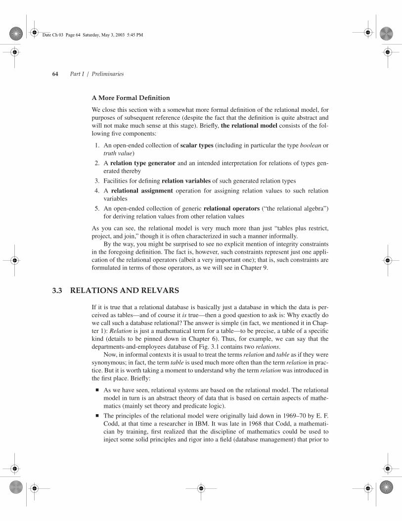
is modified by the system to become

( ( EMP WHERE SALARY > 33K ) { EMP#, ENAME, SALARY } ) WHERE SALARY < 42K ) { EMP#, SALARY }

(we have italicized the view name in the original expression and the replacement text in themodified version). The modified expression can then be simplified to just

( EMP WHERE SALARY > 33K AND SALARY < 42K ) { EMP#, SALARY }

(see Chapter 18), and this latter expression when evaluated yields the result shown earlier.In other words, the original operation against the view is effectively converted into anequivalent operation against the underlying base relvar, and that equivalent operation isthen executed in the normal way (more accurately, optimized and executed in the normalway).

By way of another example, consider the following DELETE operation:

DELETE TOPEMP WHERE SALARY < 42K ;

The DELETE that is actually executed looks something like this:

DELETE EMP WHERE SALARY > 33K AND SALARY < 42K ;

Now, the view TOPEMP is very simple, consisting as it does just of a row-and-col-umn subset of a single underlying base relvar (loosely speaking). In principle, however, aview definition, since it is essentially just a named relational expression, can be of arbi-trary complexity (it can even refer to other views). For example, here is a view whose def-inition involves a join of two underlying base relvars:

CREATE VIEW JOINEX AS ( ( EMP JOIN DEPT ) WHERE BUDGET > 7M ) { EMP#, DEPT# } ;

We will return to the whole question of view definition and view processing in Chap-ter 10.

Incidentally, we can now explain the remark in Chapter 2, near the end of Section 2.2,to the effect that the term view has a rather specific meaning in relational contexts that isnot identical to the meaning assigned to it in the ANSI/SPARC architecture. At the exter-nal level of that architecture, the database is perceived as an “external view,” defined by anexternal schema (and different users can have different external views). In relational sys-tems, by contrast, a view is, specifically, a named, derived, virtual relvar, as previouslyexplained. Thus, the relational analog of an ANSI/SPARC “external view” is (typically) acollection of several relvars, each of which is a view in the relational sense, and the“external schema” consists of definitions of those views. (It follows that views in the rela-tional sense are the relational model’s way of providing logical data independence,though once again it has to be said that today’s SQL products are sadly deficient in thisregard. See Chapter 10.)

Now, the ANSI/SPARC architecture is quite general and allows for arbitrary variabil-ity between the external and conceptual levels. In principle, even the types of data struc-tures supported at the two levels could be different; for example, the conceptual level



could be relational, while a given user could have an external view that was hierarchic.5 Inpractice, however, most systems use the same type of structure as the basis for both levels,and relational products are no exception to this general rule—views are still relvars, justlike the base relvars are. And since the same type of object is supported at both levels, thesame data sublanguage (usually SQL) applies at both levels. Indeed, the fact that a view isa relvar is precisely one of the strengths of relational systems; it is important in just thesame way as the fact that a subset is a set is important in mathematics. Note: SQL prod-ucts and the SQL standard (see Chapter 4) often seem to miss this point, however, inas-much as they refer repeatedly to “tables and views,” with the tacit implication that a viewis not a table. You are strongly advised not to fall into this common trap of taking “tables”(or “relvars”) to mean, specifically, base tables (or relvars) only.

There is one final point that needs to be made on the subject of base relvars vs. views,as follows. The base relvar vs. view distinction is frequently characterized thus:

■ Base relvars “really exist,” in the sense that they represent data that is physicallystored in the database.

■ Views, by contrast, do not “really exist” but merely provide different ways of lookingat “the real data.”

However, this characterization, though perhaps useful in informal contexts, does not accu-rately reflect the true state of affairs. It is true that users can think of base relvars as if theywere physically stored; in a way, in fact, the whole point of relational systems is to allowusers to think of base relvars as physically existing, while not having to concern themselveswith how those relvars are actually represented in storage. But—and it is a big but—thisway of thinking should not be construed as meaning that a base relvar is physically storedin any kind of direct way (e.g., as a single stored file). As explained in Section 3.2, baserelvars are best thought of as an abstraction of some collection of stored data—an abstrac-tion in which all storage-level details are concealed. In principle, there can be an arbitrarydegree of differentiation between a base relvar and its stored counterpart.6

A simple example might help to clarify this point. Consider the departments-and-employees database once again. Most of today’s relational systems would probably imple-ment that database with two stored files, one for each of the two base relvars. But there isabsolutely no logical reason why there should not be just one stored file of hierarchicstored records, each consisting of (a) the department number, name, and budget for somegiven department, together with (b) the employee number, name, and salary for eachemployee who happens to be in that department. In other words, the data can be physi-cally stored in whatever way seems appropriate (see Appendix A for a discussion of fur-ther possibilities), but it always looks the same at the logical level.

5. We will see an example of this possibility in Chapter 27.

6. The following quote from a recent book displays several of the confusions discussed in this paragraph,as well as others discussed in Section 3.3 earlier: “[It] is important to make a distinction between storedrelations, which are tables, and virtual relations, which are views ... [We] shall use relation only where atable or a view could be used. When we want to emphasize that a relation is stored, rather than a view, weshall sometimes use the term base relation or base table.” The quote is, regrettably, not at all atypical.



3.8 TRANSACTIONS

Note: The topic of this section is not peculiar to relational systems. We cover it here never-theless, because an understanding of the basic idea is needed in order to appreciate cer-tain aspects of the material to come in Part II. However, our coverage at this point isdeliberately not very deep.

In Chapter 1 we said that a transaction is a “logical unit of work,” typically involvingseveral database operations. Clearly, the user needs to be able to inform the system whendistinct operations are part of the same transaction, and the BEGIN TRANSACTION,COMMIT, and ROLLBACK operations are provided for this purpose. Basically, a transac-tion begins when a BEGIN TRANSACTION operation is executed, and terminates when acorresponding COMMIT or ROLLBACK operation is executed. For example (pseudocode):

BEGIN TRANSACTION ; /* move $$$ from account A to account B */UPDATE account A ; /* withdrawal */UPDATE account B ; /* deposit */IF everything worked fine THEN COMMIT ; /* normal end */ ELSE ROLLBACK ; /* abnormal end */END IF ;

Points arising:

1. Transactions are guaranteed to be atomic—that is, they are guaranteed (from a logi-cal point of view) either to execute in their entirety or not to execute at all,7 even if(say) the system fails halfway through the process.

2. Transactions are also guaranteed to be durable, in the sense that once a transactionsuccessfully executes COMMIT, its updates are guaranteed to appear in the database,even if the system subsequently fails at any point. (It is this durability property oftransactions that makes the data in the database persistent, in the sense of Chapter 1.)

3. Transactions are also guaranteed to be isolated from one another, in the sense that da-tabase updates made by a given transaction T1 are not made visible to any distincttransaction T2 until and unless T1 successfully executes COMMIT. COMMIT causesdatabase updates made by the transaction to become visible to other transactions;such updates are said to be committed, and are guaranteed never to be canceled. If thetransaction executes ROLLBACK instead, all database updates made by the transac-tion are canceled (rolled back). In this latter case, the effect is as if the transactionnever ran in the first place.

4. The interleaved execution of a set of concurrent transactions is usually guaranteed tobe serializable, in the sense that it produces the same result as executing those sametransactions one at a time in some unspecified serial order.

Chapters 15 and 16 contain an extended discussion of all of the foregoing points, andmuch else besides.

7. Since a transaction is the execution of some piece of code, a phrase such as “the execution of a transac-tion” is really a solecism (if it means anything at all, it has to mean the execution of an execution). How-ever, such phraseology is common and useful, and for want of anything better we will use it ourselves inthis book.



3.9 THE SUPPLIERS-AND-PARTS DATABASE

Most of our examples in this book are based on the well-known suppliers-and-parts data-base. The purpose of this section is to explain that database, in order to serve as a point ofreference for later chapters. Fig. 3.8 shows a set of sample data values; subsequent exam-ples will actually assume these specific values, where it makes any difference.8 Fig. 3.9shows the database definition, expressed in Tutorial D once again (the Tutorial D key-word VAR means “variable”). Note the primary and foreign key specifications in particu-lar. Note too that (a) several columns have data types of the same name as the column inquestion; (b) the STATUS column and the two CITY columns are defined in terms ofsystem-defined types—INTEGER (integers) and CHAR (character strings of arbitrarylength)—instead of user-defined ones. Note finally that there is an important point thatneeds to be made regarding the column values as shown in Fig. 3.8, but we are not yet in aposition to make it; we will come back to it in Chapter 5, Section 5.3, near the end of thesubsection “Possible Representations.”

The database is meant to be understood as follows:

■ Relvar S represents suppliers (more accurately, suppliers under contract). Each sup-plier has a supplier number (S#), unique to that supplier; a supplier name (SNAME),not necessarily unique (though the SNAME values do happen to be unique in Fig.3.8); a rating or status value (STATUS); and a location (CITY). We assume that eachsupplier is located in exactly one city.

■ Relvar P represents parts (more accurately, kinds of parts). Each kind of part has apart number (P#), which is unique; a part name (PNAME); a color (COLOR); a

8. For ease of reference, Fig. 3.8 is repeated as Endpaper Panel 1 at the front of the book. Note: For thebenefit of readers who might be familiar with the sample data values from earlier editions, we note thatpart P3 has moved from Rome to Oslo. The same change has also been made in Fig. 4.5 in the nextchapter.

Fig. 3.8 The suppliers-and-parts database (sample values)

S S# SNAME STATUS CITY

S1 Smith 20 LondonS2 Jones 10 ParisS3 Blake 30 ParisS4 Clark 20 LondonS5 Adams 30 Athens

P P# PNAME COLOR WEIGHT CITY

P1 Nut Red 12.0 LondonP2 Bolt Green 17.0 ParisP3 Screw Blue 17.0 OsloP4 Screw Red 14.0 LondonP5 Cam Blue 12.0 ParisP6 Cog Red 19.0 London

SP S# P# QTY

S1 P1 300S1 P2 200S1 P3 400S1 P4 200S1 P5 100S1 P6 100S2 P1 300S2 P2 400S3 P2 200S4 P2 200S4 P4 300S4 P5 400



weight (WEIGHT); and a location where parts of that kind are stored (CITY). Weassume where it makes any difference that part weights are given in pounds (but seethe discussion of units of measure in Chapter 5, Section 5.4). We also assume thateach kind of part comes in exactly one color and is stored in a warehouse in exactlyone city.

■ Relvar SP represents shipments. It serves in a sense to link the other two relvarstogether, logically speaking. For example, the first row in SP as shown in Fig. 3.8links a specific supplier from relvar S (namely, supplier S1) to a specific part fromrelvar P (namely, part P1)—in other words, it represents a shipment of parts of kindP1 by the supplier called S1 (and the shipment quantity is 300). Thus, each shipmenthas a supplier number (S#), a part number (P#), and a quantity (QTY). We assumethere is at most one shipment at any given time for a given supplier and a given part;for a given shipment, therefore, the combination of S# value and P# value is uniquewith respect to the set of shipments currently appearing in SP. Note that the databaseof Fig. 3.8 includes one supplier, supplier S5, with no shipments at all.

We remark that (as already pointed out in Chapter 1, Section 1.3) suppliers and partscan be regarded as entities, and a shipment can be regarded as a relationship between aparticular supplier and a particular part. As also pointed out in that chapter, however, arelationship is best regarded as just a special case of an entity. One advantage of relationaldatabases over all other known kinds is precisely that all entities, regardless of whether

TYPE S# ... ;TYPE NAME ... ;TYPE P# ... ;TYPE COLOR ... ;TYPE WEIGHT ... ;TYPE QTY ... ;

VAR S BASE RELATION { S# S#, SNAME NAME, STATUS INTEGER, CITY CHAR PRIMARY KEY { S# } ;

VAR P BASE RELATION { P# P#, PNAME NAME, COLOR COLOR, WEIGHT WEIGHT, CITY CHAR } PRIMARY KEY { P# } ;

VAR SP BASE RELATION { S# S#, P# P#, QTY QTY } PRIMARY KEY { S#, P# } FOREIGN KEY { S# } REFERENCES S FOREIGN KEY { P# } REFERENCES P ;

Fig. 3.9 The suppliers-and-parts database (data definition)



they are in fact relationships, are represented in the same uniform way: namely, by meansof rows in relations, as the example indicates.

A couple of final remarks:

■ The suppliers-and-parts database is clearly very simple, much simpler than any realdatabase is likely to be; most real databases will involve many more entities and rela-tionships (and, more important, many more kinds of entities and relationships) thanthis one does. Nevertheless, it is at least adequate to illustrate most of the points thatwe need to make in the rest of the book, and (as already stated) we will use it as thebasis for most—not all—of our examples as we proceed.

■ There is nothing wrong with using more descriptive names such as SUPPLIERS,PARTS, and SHIPMENTS in place of the rather terse names S, P, and SP in Figs. 3.8and 3.9; indeed, descriptive names are generally to be recommended in practice. Butin the case of the suppliers-and-parts database specifically, the relvars are referencedso frequently in what follows that very short names seemed desirable. Long namestend to become irksome with much repetition.

3.10 SUMMARY

This brings us to the end of our brief overview of relational technology. Obviously wehave barely scratched the surface of what by now has become a very extensive subject, butthe whole point of the chapter has been to serve as a gentle introduction to the much morecomprehensive discussions to come. Even so, we have managed to cover quite a lot ofground. Here is a summary of the major topics we have discussed.

A relational database is a database that is perceived by its users as a collection ofrelation variables—that is, relvars—or, more informally, tables. A relational system isa system that supports relational databases and operations on such databases, including inparticular the operations restrict, project, and join. These operations, and others likethem, are collectively known as the relational algebra,9 and they are all set-level. Theclosure property of relational systems means that the output from every operation is thesame kind of object as the input (they are all relations), which means we can write nestedrelational expressions. Relvars can be updated by means of the relational assignmentoperation; the familiar update operations INSERT, DELETE, and UPDATE can beregarded as shorthands for certain common relational assignments.

The formal theory underlying relational systems is called the relational model ofdata. The relational model is concerned with logical matters only, not physical matters. Itaddresses three principal aspects of data: data structure, data integrity, and data manipu-lation. The structural aspect has to do with relations per se; the integrity aspect has to dowith (among other things) primary and foreign keys; and the manipulative aspect has todo with the operators (restrict, project, join, etc.). The Information Principle—which we

9. We mentioned this term in the formal definition of the relational model in Section 3.2. However, wewill not start using it in earnest until we reach Chapter 6.



now observe might better be called The Principle of Uniform Representation—states thatthe entire information content of a relational database is represented in one and only oneway, as explicit values in column positions in rows in relations. Equivalently: The onlyvariables allowed in a relational database are, specifically, relvars.

Every relation has a heading and a body; the heading is a set of column-name:type-name pairs, the body is a set of rows that conform to the heading. The heading of a givenrelation can be regarded as a predicate, and each row in the body denotes a certain trueproposition, obtained by substituting certain arguments of the appropriate type for theparameters of the predicate. Note that these remarks are true of derived relations as wellas base ones; they are also true of relvars, mutatis mutandis. In other words, types are (setsof) things we can talk about, and relations are (sets of) things we say about the things wecan talk about. Together, types and relations are necessary and sufficient to represent anydata we like (at the logical level, that is).

The optimizer is the system component that determines how to implement userrequests (which are concerned with what, not how). Since relational systems thereforeassume responsibility for navigating around the stored database to locate the desired data,they are sometimes described as automatic navigation systems. Optimization and auto-matic navigation are prerequisites for physical data independence.

The catalog is a set of system relvars that contain descriptors for the various itemsthat are of interest to the system (base relvars, views, indexes, users, etc.). Users can inter-rogate the catalog in exactly the same way they interrogate their own data.

The original (given) relvars in a given database are called base relvars, and their val-ues are called base relations; a relation that is not a base relation but is obtained from thebase relations by means of some relational expression is called a derived relation (collec-tively, base and derived relations are sometimes referred to as expressible relations). Aview is a relvar whose value at any given time is such a derived relation (loosely, it can bethought of as a derived relvar); the value of such a relvar at any given time is whateverresults from evaluating the associated view-defining expression at that time. Note, there-fore, that base relvars have independent existence, but views do not—they depend on theapplicable base relvars. (Another way of saying the same thing is that base relvars areautonomous, but views are not.) Users can operate on views in exactly the same way asthey operate on base relvars, at least in theory. The system implements operations onviews by replacing references to the name of the view by the view-defining expression,thereby converting the operation into an equivalent operation on the underlying baserelvar(s).

A transaction is a logical unit of work, typically involving several database opera-tions. A transaction begins when BEGIN TRANSACTION is executed and terminateswhen COMMIT (normal termination) or ROLLBACK (abnormal termination) is exe-cuted. Transactions are atomic, durable, and isolated from one another. The interleavedexecution of a set of concurrent transactions is usually guaranteed to be serializable.

Finally, the base example for most of the book is the suppliers-and-parts database.It is worth taking the time to familiarize yourself with that example now, if you have notdone so already; that is, you should at least know which relvars have which columns andwhat the primary and foreign keys are (it is not as important to know exactly what thesample data values are!).



EXERCISES

3.1 Explain the following in your own words:

automatic navigation primary key

base relvar projection

catalog proposition

closure relational database

commit relational DBMS

derived relvar relational model

foreign key restriction

join rollback

optimization set-level operation

predicate view

3.2 Sketch the contents of the catalog relvars TABLE and COLUMN for the suppliers-and-partsdatabase.

3.3 As explained in Section 3.6, the catalog is self-describing—that is, it includes entries for thecatalog relvars themselves. Extend Fig. 3.6 to include the necessary entries for the TABLE and COL-UMN relvars themselves.

3.4 Here is a query on the suppliers-and-parts database. What does it do? What is the predicate forthe result?

( ( S JOIN SP ) WHERE P# = P# ('P2') ) { S#, CITY }

3.5 Suppose the expression in Exercise 3.4 is used in a view definition:

CREATE VIEW V AS ( ( S JOIN SP ) WHERE P# = P# ('P2') ) { S#, CITY } ;

Now consider this query

( V WHERE CITY = 'London' ) { S# }

What does this query do? What is the predicate for the result? Show what is involved on the partof the DBMS in processing this query.

3.6 What do you understand by the terms atomicity, durability, isolation, and serializability asapplied to transactions?

3.7 State The Information Principle.

3.8 If you are familiar with the hierarchic data model, identify as many differences as you canbetween it and the relational model as briefly described in this chapter.

REFERENCES AND BIBLIOGRAPHY

3.1 E. F. Codd: “Relational Database: A Practical Foundation For Productivity,” CACM 25, No. 2(February 1982). Republished in Robert L. Ashenhurst (ed.), ACM Turing Award Lectures: The FirstTwenty Years 1966–1985. Reading, Mass.: Addison-Wesley (ACM Press Anthology Series, 1987).

This is the paper Codd presented on the occasion of his receiving the 1981 ACM Turing Awardfor his work on the relational model. It discusses the well-known application backlog problem.



To quote: “The demand for computer applications is growing fast—so fast that informationsystems departments (whose responsibility it is to provide those applications) are lagging fur-ther and further behind in their ability to meet that demand.” There are two complementaryways of attacking this problem:

2. Provide IT professionals with new tools to increase their productivity.

2. Allow end users to interact directly with the database, thus bypassing the IT professionalentirely.

Both approaches are needed, and in this paper Codd gives evidence to suggest that the neces-sary foundation for both is provided by relational technology.

3.2 C. J. Date: “Why Relational?” in Relational Database Writings 1985-1989. Reading, Mass.:Addison-Wesley (1990).

An attempt to provide a succinct yet reasonably comprehensive summary of the major advan-tages of relational systems. The following observation from the paper is worth repeating here:Among all the numerous advantages of “going relational,” there is one in particular that cannotbe overemphasized, and that is the existence of a sound theoretical base. To quote: “Relationalreally is different. It is different because it is not ad hoc. Older systems, by contrast, were adhoc; they may have provided solutions to certain important problems of their day, but they didnot rest on any solid theoretical base. Relational systems, by contrast, do rest on such a base . . .which means [they] are rock solid . . . Thanks to this solid foundation, relational systemsbehave in well-defined ways; and (possibly without realizing the fact) users have a simplemodel of that behavior in their mind, one that enables them to predict with confidence what thesystem will do in any given situation. There are (or should be) no surprises. This predictabilitymeans that user interfaces are easy to understand, document, teach, learn, use, and remember.”

3.3 C. J. Date and Hugh Darwen: Foundation for Future Database Systems: The Third Manifesto(2d edition). Reading, Mass.: Addison-Wesley (2000). See also http://www.thethirdmanifesto.com,which contains certain formal extracts from the book, an errata list, and much other relevant mate-rial. Reference [20.1] is also relevant.

The Third Manifesto is a detailed, formal, and rigorous proposal for the future direction of data-bases and DBMSs. It can be seen as an abstract blueprint for the design of a DBMS and thelanguage interface to such a DBMS. It is based on the classical core concepts type, value, vari-able, and operator. For example, we might have a type INTEGER; the integer “3” might be avalue of that type; N might be a variable of that type, whose value at any given time is someinteger value (i.e., some value of that type); and “+” might be an operator that applies to inte-ger values (i.e., to values of that type). Note: The emphasis on types in particular is brought outby the book’s subtitle: A Detailed Study of the Impact of Type Theory on the Relational Modelof Data, Including a Comprehensive Model of Type Inheritance. Part of the point here is thattype theory and the relational model are more or less independent of each other. To be morespecific, the relational model does not prescribe support for any particular types (other thantype boolean); it merely says that attributes of relations must be of some type, thus implyingthat some (unspecified) types must be supported.

The term relvar is taken from this book. In this connection, the book also says this: “Thefirst version of this Manifesto drew a distinction between database values and database vari-ables, analogous to the distinction between relation values and relation variables. It also intro-duced the term dbvar as shorthand for database variable. While we still believe this distinctionto be a valid one, we found it had little direct relevance to other aspects of these proposals. Wetherefore decided, in the interests of familiarity, to revert to more traditional terminology.” This



decision subsequently turned out to be a bad one . . . To quote reference [23.4]: “With hind-sight, it would have been much better to bite the bullet and adopt the more logically correctterms database value and database variable (or dbvar), despite their lack of familiarity.” In thepresent book we do stay with the familiar term database, but we decided to do so only againstour own better judgment (somewhat).

One more point. As the book itself says: “We [confess] that we do feel a little uncomfort-able with the idea of calling what is, after all, primarily a technical document a manifesto.According to Chambers Twentieth Century Dictionary, a manifesto is a written declaration ofthe intentions, opinions, or motives of some person or group (e.g., a political party). By con-trast, The Third Manifesto is . . . a matter of science and logic, not mere intentions, opinions, ormotives.” However, The Third Manifesto was specifically written to be compared and con-trasted with two previous ones, The Object-Oriented Database System Manifesto [20.2, 25.1]and The Third-Generation Database System Manifesto [26.44], and our title was thus effec-tively chosen for us.

3.4 C. J. Date: “Great News, The Relational Model Is Very Much Alive!,” http://www.dbdebunk.com(August 2000).

Ever since it first appeared in 1969, the relational model has been subjected to an extraordinaryvariety of attacks by a number of different writers. One recent example was entitled, not at allatypically, “Great News, The Relational Model Is Dead!” This article was written as a rebuttalto this position.

3.5 C. J. Date: “There’s Only One Relational Model!” http://www.dbdebunk.com (February 2001).

Ever since it first appeared in 1969, the relational model has been subjected to an extraordinaryvariety of misrepresentation and obfuscation by a number of different writers. One recentexample was a book chapter titled “Different Relational Models,” the first sentence of whichread: “There is no such thing as the relational model for databases anymore [sic] than there isjust one geometry.” This article was written as a rebuttal to this position.



Documents

AN INTRODUCTION TO RELATIONAL DATABASES - …ce.sharif.edu/courses/84-85/2/ce384/resources/root/C. J... · · 2015-04-06AN INTRODUCTION TO RELATIONAL DATABASES 3.1 Introduction