Embed Size (px)
Citation preview

Univers
ity of
Cap
e Tow
n
An Introduction to Geotechnical Design of South African Wind Turbine Gravity
Foundations __________________________________
BY:
BYRON WADE MAWER
A thesis submitted to the University of Cape Town in partial fulfillment of the requirements for a degree in Master of Science in Engineering
Department of Civil Engineering | University of Cape Town | August 2015
The copyright of this thesis vests in the author. No quotation from it or information derived from it is to be published without full acknowledgement of the source. The thesis is to be used for private study or non-commercial research purposes only.
Published by the University of Cape Town (UCT) in terms of the non-exclusive license granted to UCT by the author.
Univers
ity of
Cap
e Tow
n

PLAGIRISM DECLARATION
Page | ii Byron Mawer MSc in Civil Engineering
Plagiarism Declaration
1. I know that plagiarism is wrong. Plagiarism is to use another’s work and pretend that it isone’s own.
2. I have used the Harvard convention for citation and referencing. Each contribution to, andquotation in, this thesis from the work(s) of other people has been attributed, and has been citedand referenced.
3. This thesis is my own work.
4. I have not allowed, and will not allow, anyone to copy my work with the intention of passingit off as his or her own work.
Signature _____________________________Date: _______________________________ 31/08/2015

Dedicated to:
Clive & Susan Mawer
For Their endless love and support in whatever I pursue

ACKNOWLEDGEMENTS
Page | iv Byron Mawer MSc in Civil Engineering
Acknowledgements This dissertation would not have been possible without the guidance and input from a number of people and organizations, and I would like to express my thanks: a) Firstly, to my supervisor, Dr. Denis Kalumba. The guidance and willingness to help on even the most minor problems I have encountered has been greatly appreciated and extremely helpful. This thesis would never have been completed without your help,
b) To Dr. Gabrielle Wotjowitz of Aurecon, for her willingness to provide me with information and her detailed guidance in what was an extremely complex topic, even though she had no obligation to assist. Your help was invaluable,
c) To my bursars, Jeffares & Green Consulting Engineers, specifically Ms. Jan Norris, Mr. Richard Fyvie and Mr. Michael Manson-Kullin for providing me with insight and valuable information when required,
d) To the Department of Civil Engineering at UCT, for the financial support and for allowing me to follow this field of research,
e) Mr. Patrick Beales of Kantey & Templar Consulting Engineers, for his help and guidance when addressing issues that were far out of my field of expertise and his willingness to respond to even the simplest questions,
f) Mr. Charles Warren-Codrington and Mr. Frans van der Merwe of SMEC, for their guidance and supply of information even when extremely busy and with little expectation of benefit for themselves,
g) My fellow researchers in the UCT Geotechnical Engineering Research Group, for always allowing me to bounce ideas off of them, or allowing me to spend hours rattling off about how interesting wind turbines actually are,
h) My proof reading team, consisting of Mr. Duncan McKune, Ms. Danica Davies, Mr. Craig Bedingfield, Mr. Andrew Robinson and Mr. Roberto Talloti. I appreciate the input into taking my dissertation to the next level,
i) My extremely supportive girlfriend, who didn’t mind when I had to work weekends and surprised me with study snacks when I most needed them,
j) Finally, my family and friends, for their love and support over the last two years.
ABSTRACT
Page | v Byron Mawer MSc in Civil Engineering
Abstract With the increasing pressure on global governments to pursue more green and renewable energy production measures, wind based solutions have progressed into one of the most dominant development areas in the global renewable energy sector. In South Africa, with notable deficiencies in reliable energy supply, a number of wind projects have been planned in order to relieve the pressure on the nation’s volatile reserves. With a lack of exposure to the complexities of wind turbine foundation design in Africa, this research aimed to present a methodology for the geotechnical design of gravity footings for these structures, specific to SA soil conditions and policies. To understand the implications of the main aim of the study, the current scope for renewable energy project uptake in South Africa was summarized, highlighting the scope and growth potential legislated by the Renewable Energy Independent Power Producer Procurement Programme. This summary indicates the current development corridors for wind projects that fall along the Eastern and South West coasts of the country and discusses the economics of wind farm ventures and their inherent ability to attract local and international investment. Additionally to this, topics including a basic introduction to turbine mechanics, tower and foundation types, and the effect of loading actions on the dynamic soil reactions, were presented. This was concluded by discussing gravity footings in context to other foundation types, and their advantages for use in these types of developments. With this understanding, the main research outcome was addressed by selecting three representative sites from each of the major wind development corridors, and using them as practical examples. These were resultantly named the Western Cape, Eastern Cape and Karoo sites. Soil profiles and properties were assumed based on site investigation data from real projects from each of these corridors and this data was compiled, discussed and used in the planning of three designs for each respective site. In this way, a geotechnical methodology was created addressing the critical criteria that require consideration for the construction of turbine base structures. These considerations included appropriate site investigation methods particularly suited for wind turbine foundations, such as Continuous Surface Wave testing, as well as bearing capacity calculations according to theories suggested by the DNV/Risφ (2002) guidelines and site-specific bearing capacity theories. Settlement concerns were addressed through the analysis of immediate elastic settlement beneath a foundation using a general elastic solution, a non-linear stepwise method as well as the computer software, Settle 3D. Unique to wind structures, the criterion of soil stiffness was considered in order address the structure’s global resistance to rotation, caused by the high overturning moments inherent in these systems. The effect that the calculated finite soil stiffness has on the assumptions in computing the natural frequency of the system was also investigated. Finally, additional concerns such as the effect of gapping, issues with designing on pedogenic soils such as calcrete, as well as the use of the finite element method in the planning of turbine foundations, were discussed. In concluding the study, a general design process for engineers tasked with planning gravity footings for wind turbines subject to local soil conditions was presented.

TABLE OF CONTENTS
Page | vi Byron Mawer MSc in Civil Engineering
Table of Contents PLAGIARISM DECLARATION ......................................................................................... II
ACKNOWLEDGEMENTS................................................................................................. IV
ABSTRACT ............................................................................................................................ V
TABLE OF CONTENTS..................................................................................................... VI
NOMENCLATURE ............................................................................................................. IX
LIST OF FIGURES ............................................................................................................. XI
LIST OF EQUATIONS .................................................................................................... XIII
LIST OF TABLES .............................................................................................................. XV
1. INTRODUCTION .......................................................................................................... 1
1.1 BACKGROUND TO STUDY ........................................................................................... 1
1.2 SOUTH AFRICAN WIND TURBINE FOUNDATION DESIGN ............................................ 2
1.2.1 Energy Crisis in South Africa ............................................................................... 2
1.2.2 Limitations of Literature ....................................................................................... 3
1.2.3 Limitation to exposure in Africa ........................................................................... 4
1.2.4 Possible Benefits of Research ............................................................................... 5
1.3 THEMES AND OBJECTIVES OF WORK.......................................................................... 5
1.3.1 Problem Statement ................................................................................................ 5
1.3.2 Objectives of Research ......................................................................................... 5
1.3.3 Scope and Limitations .......................................................................................... 6
1.4 THESIS STRUCTURE.................................................................................................... 6
2. WIND ECONOMY IN SOUTH AFRICA .................................................................... 9
2.1 BACKGROUND TO SOUTH AFRICAN ENERGY LANDSCAPE ......................................... 9
2.2 RENEWABLE ENERGY IN SOUTH AFRICA ................................................................. 10
2.3 WIND ENERGY AND PROJECT UPTAKE ..................................................................... 12
2.3.1 Siting Criteria ...................................................................................................... 13
2.3.2 Project Uptake ..................................................................................................... 14
3. WIND TURBINES ........................................................................................................ 16
3.1 INTRODUCTION ........................................................................................................ 16
3.2 GENERATION OF POWER FROM WIND TURBINES ...................................................... 16
3.3 TYPES OF WIND TURBINE INFRASTRUCTURE ........................................................... 18
3.3.1 Onshore vs. Offshore .......................................................................................... 18
3.3.2 Types of Onshore Wind Turbines ....................................................................... 19
3.4 HORIZONTAL AXIS WIND TURBINES ........................................................................ 20
3.4.1 Structure .............................................................................................................. 20
TABLE OF CONTENTS
Page | vii Byron Mawer MSc in Civil Engineering
3.4.2 Hub Height .......................................................................................................... 22
3.4.3 Design Materials ................................................................................................. 23
3.5 LOADING .................................................................................................................. 27
3.5.1 Wind Turbine Aerodynamics .............................................................................. 27
3.5.2 Operational States ............................................................................................... 31
3.5.3 Control Measures ................................................................................................ 32
3.5.4 Dynamic Soil Loading Considerations ............................................................... 33
3.6 FOUNDATION TYPES ................................................................................................ 38
3.6.1 Gravity Foundations ........................................................................................... 39
3.6.2 Piled Foundations ............................................................................................... 39
3.6.3 Caissons & Prestressed Cylinder Design ............................................................ 39
3.6.4 Rock Anchored ................................................................................................... 40
4. SOUTH AFRICAN GEOTECHNICAL PRACTICE ............................................... 42
4.1 INTRODUCTION ........................................................................................................ 42
4.2 SITE INVESTIGATIONS .............................................................................................. 43
4.2.1 Soil Parameters for Design ................................................................................. 43
4.2.2 Parameters Required ........................................................................................... 44
4.2.3 Investigation Methods ......................................................................................... 45
4.2.4 Other Investigations ............................................................................................ 52
4.2.5 Rock Properties ................................................................................................... 54
4.3 SOUTH AFRICAN SOIL CONDITIONS ......................................................................... 59
4.3.1 Eastern Cape Wind Farm .................................................................................... 60
4.3.2 Western Cape Wind Farm ................................................................................... 64
4.3.3 Karoo Wind Farm ............................................................................................... 67
5. GEOTECHNICAL DESIGN METHODOLOGY ..................................................... 71
5.1 DESIGN CODES & REFERENCES ............................................................................... 71
5.1.1 DNV/Risφ (2002) ............................................................................................... 71
5.1.2 Manufacturers Technical Guidelines .................................................................. 72
5.1.3 IEC 61400-1 ........................................................................................................ 73
5.1.4 Svensson (2008) .................................................................................................. 73
5.1.5 Warren-Codrington (2013) ................................................................................. 74
5.1.6 Das (2011) ........................................................................................................... 74
5.2 LOADING .................................................................................................................. 75
5.2.1 Types of Loads .................................................................................................... 75
5.2.2 Factors affecting Loading ................................................................................... 77
5.2.3 Load Cases & Design Situations ........................................................................ 78
5.2.4 Dimensioning & Gravity Load ........................................................................... 81
5.2.5 Loads used in design ........................................................................................... 83
5.3 BEARING CAPACITY ................................................................................................. 84
5.3.1 Introduction ......................................................................................................... 84

TABLE OF CONTENTS
Page | viii Byron Mawer MSc in Civil Engineering
5.3.2 Effective Area & Eccentricity ............................................................................. 84
5.3.3 Correction for Mz ................................................................................................ 88
5.3.4 Extremely Eccentric Load .................................................................................. 88
5.3.5 DNV/Risφ (2002) Bearing Capacity Calculation ............................................... 89
5.3.6 Site Specific Bearing Capacity Calculations ...................................................... 98
5.3.7 Discussion ......................................................................................................... 107
5.3.8 Overturning & Sliding ...................................................................................... 111
5.4 SETTLEMENT .......................................................................................................... 114
5.4.1 Introduction ....................................................................................................... 114
5.4.2 Foundation Rigidity & Stress Distribution ....................................................... 115
5.4.3 Traditional Elastic Solution for Settlement of Foundation ............................... 118
5.4.4 Archer (2014) Non-Linear Step Wise Method ................................................. 122
5.4.5 Settle 3D ........................................................................................................... 128
5.4.6 Discussion & Summary .................................................................................... 131
5.5 FOUNDATION STIFFNESS ........................................................................................ 134
5.5.1 Introduction ....................................................................................................... 134
5.5.2 Types of Soil Stiffness ...................................................................................... 135
5.5.3 Eastern Cape Wind Farm .................................................................................. 138
5.5.4 Western Cape Wind Farm ................................................................................. 139
5.5.5 Karoo Wind Farm ............................................................................................. 140
5.5.6 Discussion ......................................................................................................... 140
5.6 NATURAL FREQUENCY EFFECTS ............................................................................ 142
5.6.1 Introduction ....................................................................................................... 142
5.6.2 Theory ............................................................................................................... 142
5.6.3 Results – Natural Frequency by foundation size .............................................. 147
5.6.4 Results – Natural Frequency plots within frequency range .............................. 149
5.6.5 Results – Dynamic amplification effects .......................................................... 152
5.6.6 Discussion & Summary .................................................................................... 153
5.7 OTHER CONSIDERATIONS....................................................................................... 156
5.7.1 Foundations on Pedogenic Soils ....................................................................... 156
5.7.2 Finite Element Modelling in Design ................................................................. 158
5.7.3 Gapping ............................................................................................................. 159
6. CONCLUSION ........................................................................................................... 161
6.1 SUMMARY OF DESIGN CRITERIA RESULTS ............................................................. 161
6.2 GENERAL DESIGN METHODOLOGY ........................................................................ 163
7. RECOMMENDATIONS ............................................................................................ 164
8. REFERENCES ............................................................................................................ 165

NOMENCLATURE
Page | ix Byron Mawer MSc in Civil Engineering
Nomenclature AcronymsASCE – American Society of Civil
Engineers ATS – Advanced Tower System BS – British Standard CBR – California Bearing Ratio CCGT – Combined Cycle Gas Turbine COP17 – Conference of the Parties 17 CPT – Cone Penetration Test CSIR – Council for Scientific and
Industrial Research CSP – Concentrated Solar Power CSW – Continuous Surface Wave DAF – Dynamic Amplification Factor DCP – Dynamic Cone Penetrometer DLC – Design Load Case DMT – Dilatometer Test DNV – Det Nortske Veritas DoE – Department of Energy DPSH – Dynamic Probe Super Heavy EC – Eastern Cape EIA – Environmental Impact Assessment EWM – Extreme Wind Model FE – Finite Elements FEM – Finite Element Method FLS – Fatigue Limit State FOS – Factor of Safety GE – General Electric GSI – Geological Strength Index H-B – Hoek-Brown HAWT – Horizontal Axis Wind Turbine IEC – International Electro-Technical
Commission IEP – Integrated Energy Plan IRP – Integrated Resource Plan L.C – Load Center LC – Load Case
MARS – Mageen Air Rotor System MDD – Maximum Dry Density NERSA – National Energy Regulator of
South Africa NMC – Natural Moisture Content NWM – Normal Wind Model OCGT – Open Cycle Gas Turbine OMC – Optimum Moisture Content PMT – Pressuremeter Test PV – Photovoltaic REFIT – Renewable Energy Feed-In Tariff REIPPPP – Renewable Energy Independent
Power Producers Procurement Programme
RQD – Rock Quality Designation SA – South Africa SAER – South African Energy Regulator SANS – South African National Standards SASW – Spectral Analysis of Surface
Waves SAWEA – South African Wind Energy
Association SEA – Strategic Environmental
Assessment SG – Specific Gravity SLS – Serviceability Limit State SPT – Standard Penetration Test TMH – Technical Methods for Highways UCS – Unconfined Compressive Strength UDL – Uniform Distributed Load ULS – Ultimate Limit State UN – United Nations US – United States VAWT – Vertical Axis Wind Turbine WASA – Wind Atlas of South Africa WC – Western Cape
Geotechnical Symbols φ’ – Drained Internal Angle of Soil Friction su – Undrained Shear Strength cu – Undrained Cohesion c’ – Drained Cohesion
Other Symbols MW – Mega Watt kW – Kilo Watt kWh – Kilo Watt hour B.C. – Before Christ

NOMENCLATURE
Page | x Byron Mawer MSc in Civil Engineering
Geotechnical Symbols (cntd.) Aeff/A’ – Effective Area B – Breadth of Footing Be – Equivalent Breadth Beff/B’ – Effective Breadth CM – Linear spring stiffness adjustment D – Disturbance Factor (H-B) Df – Depth of Embedment DD – Dry Density ds – Rock Joint Spacing e – Eccentricity E0 – Small Strain Elastic Modulus E – Strain Adjusted Elastic Modulus Em – Rock Mass Modulus Ev’ – Modulus of Compressibility G0 – Small Strain Shear Modulus Gmax – Small Strain Shear Modulus G – Strain Adjusted Shear Modulus If – Settlement Influence Factor Is – Point Load Index KH – Lateral Soil Stiffness KV – Lateral Soil Stiffness K – Lateral Soil Stiffness LL – Liquid Limit L’ – Effective Length Leff/Le – Effective Length Mi – Intact Rock Constant qact – actual experienced pressure qall – allowable bearing capacity qover – overburden pressure qult – ultimate bearing capacity Q – Applied Load PL – Plastic Limit ST – Total Settlement Se – Elastic Settlement Sc – Consolidation Settlement Ss – Secondary Consolidation Settlement
SL – Shrinkage Limit ς – Damping Ratio for soil v – Poisson’s Ratio W.T. – Water Table – Unit weight of soil z – Depth to Water Table Other Symbols (cntd.) 1P – First blade 2P – Blade passing frequency (2
blades) 3P – Blade passing frequency (3
blades) – Ratio of frequency to natural
frequency Dfooting – Diameter of footing Dsteel cage – Diameter of steel cage ε – strain in soil body Fres – Resultant force in x,y directions Fres’ – Resultant force adjusted for torsion Fz – Vertical force due to weight and
wind action Hz – Hertz I – Moment of inertia k – Global stiffness value m – Mass of system fn – First natural frequency of system Mres – Resultant moment about x,y axes Mz – Torsional moment about z- axis R – Radius of footing RPM – Revolutions per minute σ – stress in soil body t – Thickness of tower wall tfooting – thickness of footing base – mass per meter for turbine tower ς – damping ratio for dynamic loading
Bearing Capacity Factors Nq – Bearing capacity factor for overburden Nc – Bearing capacity factor for cohesion N – Bearing capacity factor for wedge sq – Shape factor for overburden sc – Shape factor for cohesion s – Shape factor for wedge
dq – Depth factor for overburden dc – Depth factor for cohesion d – Depth factor for wedge iq – Inclination factor for overburden ic – Inclination factor for cohesion i – Inclination factor for wedge

LIST OF FIGURES
Page | xi Byron Mawer MSc in Civil Engineering
List of Figures Figure 1-1: Jeffery’s Bay Wind Farm, Jeffery’s Bay RSA Pg 1 Figure 1-2: South African Energy Demand for first third of 2015 Pg 3 Figure 1-3: Current planned and completed wind energy projects in Africa Pg 4 Figure 2-1: Division of South African Electricity Generation Capacity in 2012 Pg 9 Figure 2-2: Distribution & concentration of wind over South Africa Pg 12 Figure 2-3: REIPPPP Projects overlaid with Wind Energy Potential for Western Cape Pg 14 Figure 3-1: Power Curve for a Vestas V126-3.0MW Wind Turbine Pg 17 Figure 3-2: Onshore vs. Offshore Wind Turbine Foundations Pg 19 Figure 3-3: Wind Turbine Structures by type - a) HAWT, b) VAWT, c) MARS Pg 20 Figure 3-4: Physical components of a HAWT structure Pg 21 Figure 3-5: Change in Power Generation with Increasing Hub Height and Rotor Size Pg 22 Figure 3-6: Hybrid wind turbine tower elements: a) ATS, b) Max Bőgl, c) ENERCON design Pg 25 Figure 3-7: Construction of a precast concrete onshore HAWT tower Pg 26 Figure 3-8: Drag and Lift forces on a plate placed in fluid flow Pg 28 Figure 3-9: Principles of drag and lift as it applies to aircraft wings Pg 28 Figure 3-10: Aerodynamic principles behind operation of a HAWT Pg 30 Figure 3-11: Power control measures (a) active stall, (b) passive stall and (c) pitch controlled. Pg 32 Figure 3-12: Changes in soil response with increasing strain Pg 34 Figure 3-13: Hysteretic loop showing shear stress-strain for soils under dynamic loading Pg 35 Figure 3-14: Popular Onshore Wind Turbine foundation designs Pg 38 Figure 4-1: Geotechnical Design Methodology Outline for Chapter Pg 42 Figure 4-2: SPT sampler vs. DPSH Cone Setup Pg 45 Figure 4-3: Point Load Index test correlations with UCS value for Rocks Pg 48 Figure 4-4: CSW test apparatus and function diagram Pg 51 Figure 4-5: Drained modulus of compressibility (Ev’) for sands Pg 51 Figure 4-6: Example of the formation of rutting on a poorly designed haul road Pg 54 Figure 4-7: Failure mechanisms in rock under concentrated load Pg 56 Figure 4-8: Mohr-Coulomb curve generated for rock by RocLab software Pg 58 Figure 4-9: SA Wind Corridor overlain on hybrid topographical map with wind speed Pg 60 Figure 4-10: Eastern Cape Wind Farm Soil Profile and Description Pg 61 Figure 4-11: CSW Test Results for Eastern Cape Wind Farm Pg 63 Figure 4-12: Western Cape Wind Farm Soil Profile Pg 65 Figure 4-13: CSW Test Results for Western Cape Wind Farm Pg 67 Figure 4-14: Karoo Wind Farm Soil Profile Pg 68 Figure 4-15: CSW Test Results for Karoo Wind Farm Pg 70 Figure 5-1: Simplified loading on Wind Turbine Structure for design Pg 76 Figure 5-2: Spacing of wind turbines on site to increase aerodynamic efficiency Pg 77 Figure 5-3: Plan and Profile views of (1,2a) circular and (1,2b) square foundations Pg 82 Figure 5-4: Calculation of effective area of circular shaped gravity footing Pg 83
LIST OF FIGURES
Page | xii Byron Mawer MSc in Civil Engineering
Figure 5-5: Calculation of effective area for square shaped gravity footings – S1 Pg 87 Figure 5-6: Calculation of effective area for square shaped gravity footings - S2 Pg 87 Figure 5-7: Formation of failure plane over relatively rigid layer compared with soil Pg 98 Figure 5-8: Mandel & Salencon (1972) predictions of Nq* for soils supported by rigid base Pg 99 Figure 5-9: Meyerhof & Hanna (1978) method for weaker layer overlying stronger soil Pg 101 Figure 5-10: Bearing capacity calculations for foundations on rock Pg 103 Figure 5-11: Graph showing bearing capacity values for Group 2 rocks Pg 106 Figure 5-12: Diagram depicting the calculation of overturning factor of safety Pg 111 Figure 5-13: Effect of contact pressure on settlement distribution – a) flexible footing on cohesive soil, b) flexible footing on granular soil, c) rigid footing on cohesive soil, and d) rigid footing on granular footing Pg 116 Figure 5-14: Stress distribution at a point under circular distributed load Pg 117 Figure 5-15: Settle 3D settlement predictions for Eastern Cape Wind Farm Pg 129 Figure 5-16: Settle 3D settlement predictions for Western Cape Wind Farm Pg 130 Figure 5-17: Settle 3D settlement predictions for Karoo Wind Farm Pg 130 Figure 5-18: Campbell Diagram for frequency effect on turbine design Pg 135 Figure 5-19: Foundation soil stiffness components Pg 136 Figure 5-20: Link between total & differential settlements and angular distortion of footings Pg 141 Figure 5-21: Simplified beam lumped parameter system Pg 143 Figure 5-22: Simplified wind turbine lumped parameter model Pg 143 Figure 5-23: Working frequency ranges for GE 1.6 MW turbine Pg 146 Figure 5-24: Working frequency ranges for Vestas 3MW turbine Pg 146 Figure 5-25: Natural frequency for infinite and finite stiffness for Eastern Cape Wind Farm Pg 149 Figure 5-26: Natural frequency for infinite and finite stiffness for Western Cape Wind Farm Pg 150 Figure 5-27: Natural frequency for infinite and finite stiffness for Karoo Wind Farm Pg 151 Figure 5-28: Effect on Dynamic Amplification for Eastern Cape Wind Farm (R=10) Pg 152 Figure 5-29: Effect on Dynamic Amplification for Western Cape Wind Farm (R=10) Pg 152 Figure 5-30: Effect on Dynamic Amplification for Karoo Wind Farm (R=9) Pg 152 Figure 5-31: Distribution of pedocrete soils in South Africa. Pg 157 Figure 5-32: An example of FE model of wind turbine gravity foundation Pg 159 Figure 5-33: Depiction of the maximum allowed gapping and the effect on pressure Pg 160 Figure 6-1: Design Methodology for wind turbine gravity foundations in SA soil conditions Pg 163

LIST OF EQUATIONS
Page | xiii Byron Mawer MSc in Civil Engineering
List of Equations Equation 1: Rated Power Output by wind turbine structures Pg 16 Equation 2: Generated wind speed from hub to rotor tip Pg 29 Equation 3: Secant modulus relationship Pg 36 Equation 4: Calculation of Damping Ratio in Soils Pg 36 Equation 5: SPT N Correlation with DPSH for WC Soils Pg 46 Equation 6: Relationship between shear modulus and elastic modulus Pg 48 Equation 7: Relationship between shear modulus shear wave velocity Pg 50 Equation 8: Max and Minor Stresses (H-B) Pg 57 Equation 9: Normal stress calculation using H-B criteria Pg 57 Equation 10: Shear stress calculation using H-B criteria Pg 57 Equation 11: Calculation of effective H-B cohesion value Pg 57 Equation 12: Calculation of effective H-B phi value Pg 57 Equation 13: Calculation of rock mass modulus i) Pg 58 Equation 14: Calculation of rock mass modulus ii) Pg 58 Equation 15: Eccentricity calculation for bearing capacity Pg 84 Equation 16: Effective length calculations for bearing capacity Pg 84 Equation 17: Effective area calculation for circular foundations Pg 85 Equation 18: Effective area calculation for rectangular foundations - Scenario 1 Pg 86 Equation 19: Equation for correcting Mz into H’ Pg 88 Equation 20: Additional Extremely Eccentric Load bearing capacity check Pg 88 Equation 21: Hansen’s bearing capacity equation Pg 90 Equation 22: Max pressure experienced due to eccentric load Pg 92 Equation 23: Min pressure experienced due to eccentric load Pg 92 Equation 24: Mandel & Salencon (1972) bearing capacity equation Pg 99 Equation 25: Meyerhof & Hanna (1978) bearing capacity equation Pg 101 Equation 26: Adapted Terzaghi Bearing capacity equation Pg 103 Equation 27: RQD modification by Bowles (1989) Pg 103 Equation 28: Factor of safety against overturning – general Pg 111 Equation 29: Factor of safety against overturning – Vestas V112 3MW Pg 111 Equation 30: Factor of safety against sliding Pg 111 Equation 31: Total settlement equation Pg 114 Equation 32: Bounsineesq equation for vertical stress under a circular footing Pg 117 Equation 33: Bounsineesq equation for radial stress under a circular footing Pg 117 Equation 34: Derivation of traditional elastic solution Pg 118 Equation 35: Settlement formula for general elastic response Pg 118 Equation 36: Vertical strain using principal stresses Pg 123 Equation 37: Shear stress adaptation using vertical strain Pg 123

LIST OF EQUATIONS
Page | xiv Byron Mawer MSc in Civil Engineering
Equation 38: Total settlement using Archer (2014) method Pg 123 Equation 39: Basic natural frequency equation for structure Pg 134 Equation 40: Formulation of effective stiffness of system Pg 144 Equation 41: Stiffness for simplified cantilever beam Pg 144 Equation 42: Effective stiffness of simplified wind turbine system Pg 144 Equation 43: Natural frequency with Byrne (2011) finite stiffness assumption Pg 144 Equation 44: Natural frequency with Byrne (2011) infinite stiffness assumption Pg 144 Equation 45: Natural frequency with van der Tempel (2002) finite stiffness assumption Pg 145 Equation 46: Natural frequency with van der Tempel (2002) infinite stiffness assumption Pg 145 Equation 47: Dynamic amplification factor for undamped system Pg 147 Equation 48: Dynamic amplification factor for damped system Pg 147 Equation 49: Stiffness formula adjustment for gapping by Vestas (2011) Pg 160

LIST OF TABLES
Page | xv Byron Mawer MSc in Civil Engineering
List of Tables Table 2-1: 2013 Adjusted IRP Policy Plan for Infrastructure Planning Pg 10 Table 2-2: REIPPPP Rated Capacity Infrastructure Awards for each bidding round Pg 11 Table 2-3: Wind Farm Project Uptake since REIPPPP establishment in 2010 Pg 15 Table 3-1: Advantages & Disadvantages of Onshore & Offshore Wind Turbines Pg 18 Table 3-2: Stiffness degradation curves for calculation of secant shear modulus G Pg 37 Table 4-1: Table summarizing testing methods for determining dynamic soil parameters Pg 49 Table 4-2: Frequently used SA soil tests linked to parameters required for design Pg 52 Table 4-3: Summary of Soil Data for Eastern Cape Wind Farm Pg 62 Table 4-4: Available soil property data for Western Cape Wind Farm site Pg 66 Table 4-5: Soil Properties for Karoo Wind Farm Rocks from lab tests and H-B method Pg 69 Table 5-1: Table 2 extracted from IEC61400-1 for load cases and combinations Pg 79 Table 5-2: Loads acting at tower base for GE 1.6MW turbine Pg 80 Table 5-3: Loads acting at tower base for Vestas 3MW turbine Pg 80 Table 5-4: Assumed dimensions for square and circular footings Pg 81 Table 5-5: Volume and Weights of Footings Pg 82 Table 5-6: Loading cases used in the design excl. foundation weight Pg 83 Table 5-7: Values of Fz incl. foundation weight for each load case per foundation type (EC) Pg 83 Table 5-8: Eccentricity values for square and circular footings for each load case Pg 85 Table 5-9: Effective area and dimensions for circular foundations Pg 86 Table 5-10: Effective Fres for each footing shape incl. torsional moment Pg 88 Table 5-11: Extremely eccentric load check for limit B/6 Pg 89 Table 5-12: Extremely eccentric load check for limit 0.3B Pg 89 Table 5-13: Factors for Hansen bearing capacity calculations for rectangular footing Pg 91 Table 5-14: Results from Hansen bearing capacity calculations for rectangular footing Pg 92 Table 5-15: Factors for Hansen bearing capacity calculations for circular footing Pg 93 Table 5-16: Results from Hansen bearing capacity calculations for a circular footing Pg 93 Table 5-17: Summary of loads, eccentricities and effective areas for WC Wind Farm Pg 94 Table 5-18: Results of bearing capacity calculations for WC Wind Farm Pg 95 Table 5-19: Loads, eccentricities and effective areas of footings for Karoo Wind Farm Pg 96 Table 5-20: Results of bearing capacity calculations for Karoo Wind Farm Pg 97 Table 5-21: Values used in calculation of bearing capacity using Mandel & Salencon method Pg 100 Table 5-22: Properties and factors calculated using Hansen’s method Pg 102 Table 5-23: Results of bearing capacity calculations using Stagg & Zienkiewicz method Pg 104 Table 5-24: Groupings of weak and broken rocks Pg 105 Table 5-25: Results of bearing capacity calculations using Eurocode 7 empirical method Pg 105 Table 5-26: Allowable bearing capacity values compared with actual applied pressures Pg 107 Table 5-27: Summary of design dimensions for Eastern Cape Wind Farm footings Pg 108 Table 5-28: Summary of bearing capacity results for Eastern Cape Wind Farm footings Pg 108

LIST OF TABLES
Page | xvi Byron Mawer MSc in Civil Engineering
Table 5-29: Summary of design dimensions for Western Cape Wind Farm footings Pg 109 Table 5-30: Summary of bearing capacity results for Western Cape Wind Farm footings Pg 109 Table 5-31: Summary of design dimensions for Karoo Wind Farm footings Pg 110 Table 5-32: Summary of bearing capacity results for Karoo Wind Farm footings Pg 110 Table 5-33: Summary of design dimensions and values for all sites Pg 110 Table 5-34: Results of Overturning and Sliding checks for Eastern Cape Wind Farm Pg 112 Table 5-35: Results of Overturning and Sliding checks for Western Cape Wind Farm Pg 112 Table 5-36: Results of Overturning and Sliding checks for Karoo Wind Farm Pg 113 Table 5-37: Influence Factor (If) for rigid and flexible foundations Pg 118 Table 5-38: Summary of E values over Eastern Cape Wind Farm soil profile Pg 119 Table 5-39: Summary of E values over Western Cape Wind Farm soil profile Pg 120 Table 5-40: Summary of E values over Karoo Wind Farm soil profile Pg 121 Table 5-41: Summary of soil layers and assigned E0 value for Eastern Cape Wind Farm Pg 124 Table 5-42: Summary of calculation of stresses, strains for EC Wind Farm Pg 124 Table 5-43: Summary of calculation of settlement for EC Wind Farm Pg 125 Table 5-44.1: Summary of results of Archer (2014) stress-strain calcs for WC site Pg 125 Table 5-44.2 Summary of results of Archer (2014) stress-strain calcs for WC site Pg 126 Table 5-44.3: Summary of results of Archer (2014) stress-strain calcs for WC site Pg 126 Table 5-45.1: Summary of results of Archer (2014) settlement prediction for Karoo WF Pg 126 Table 5-45.2: Summary of results of Archer (2014) settlement prediction for Karoo WF Pg 127 Table 5-45.3: Summary of results of Archer (2014) settlement prediction for Karoo WF Pg 127 Table 5-46: Summary of settlement predictions by method for 3 representative sites Pg 131 Table 5-47: Summary of settlement design values for sites investigated Pg 133 Table 5-48 a): Equations for the calculation of soil stiffness Pg 137 Table 5-48 b): Equations for the calculation of soil stiffness Pg 138 Table 5-49: Manufacturers limits on soil stiffness for rigidity assumption to apply Pg 138 Table 5-50: Results of stiffness checks for Eastern Cape Wind Farm Pg 139 Table 5-51: Results of stiffness checks for Western Cape Wind Farm Pg 139 Table 5-52: Results of stiffness checks for Karoo Wind Farm Pg 140 Table 5-53: Eurocode 7 limits on settlement and angular distortions Pg 141 Table 5-54: Summary of properties and parameters used in natural frequency estimation. Pg 145 Table 5-55: Summary of operating speeds and working frequencies for range of turbines Pg 146 Table 5-56: Natural frequency excl. foundation stiffness for investigation sites Pg 147 Table 5-57: Natural frequency incl. foundation stiffness for Eastern Cape Wind Farm Pg 148 Table 5-58: Natural frequency incl. foundation stiffness for Western Cape Wind Farm Pg 148 Table 5-59: Natural frequency incl. foundation stiffness for Karoo Wind Farm Pg 148 Table 5-60: % Difference in Natural Frequency due to increasing foundation size (EC) Pg 154 Table 5-61: % Difference in Natural Frequency due to increasing foundation size (Karoo) Pg 154 Table 5-62: % Difference in Natural Frequency due to increasing foundation size (WC) Pg 155

INTRODUCTION
Page | 1 Byron Mawer MSc in Civil Engineering
1. INTRODUCTION
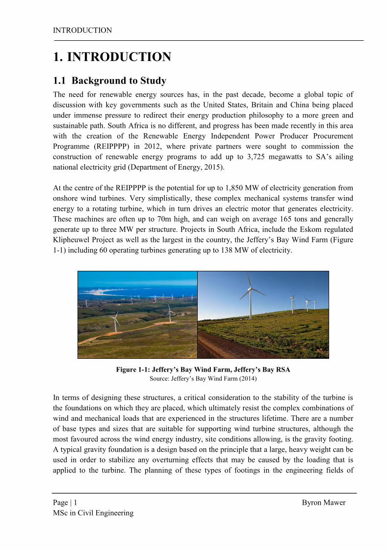
1.1 Background to Study The need for renewable energy sources has, in the past decade, become a global topic of discussion with key governments such as the United States, Britain and China being placed under immense pressure to redirect their energy production philosophy to a more green and sustainable path. South Africa is no different, and progress has been made recently in this area with the creation of the Renewable Energy Independent Power Producer Procurement Programme (REIPPPP) in 2012, where private partners were sought to commission the construction of renewable energy programs to add up to 3,725 megawatts to SA’s ailing national electricity grid (Department of Energy, 2015). At the centre of the REIPPPP is the potential for up to 1,850 MW of electricity generation from onshore wind turbines. Very simplistically, these complex mechanical systems transfer wind energy to a rotating turbine, which in turn drives an electric motor that generates electricity. These machines are often up to 70m high, and can weigh on average 165 tons and generally generate up to three MW per structure. Projects in South Africa, include the Eskom regulated Klipheuwel Project as well as the largest in the country, the Jeffery’s Bay Wind Farm (Figure 1-1) including 60 operating turbines generating up to 138 MW of electricity.
Figure 1-1: Jeffery’s Bay Wind Farm, Jeffery’s Bay RSA Source: Jeffery’s Bay Wind Farm (2014)
In terms of designing these structures, a critical consideration to the stability of the turbine is the foundations on which they are placed, which ultimately resist the complex combinations of wind and mechanical loads that are experienced in the structures lifetime. There are a number of base types and sizes that are suitable for supporting wind turbine structures, although the most favoured across the wind energy industry, site conditions allowing, is the gravity footing. A typical gravity foundation is a design based on the principle that a large, heavy weight can be used in order to stabilize any overturning effects that may be caused by the loading that is applied to the turbine. The planning of these types of footings in the engineering fields of
INTRODUCTION
Page | 2 Byron Mawer MSc in Civil Engineering
geotechnics and structures, are governed by a country’s design standards such as the Eurocode series in Europe, the ASCE standards in North America and the SANS in South Africa. Due to the unique type of loading and load combinations that act on a wind turbine structure, none of the aforementioned codes are able to deal specifically with all critical aspects that ensure a wind turbine foundation is structurally safe. In 2002, the Det Nortske Veritas and the Risφ National Laboratory in Denmark collaborated in order to publish a document entitled, “Guidelines for the Design of Wind Turbines” which has been adapted as a guideline in most European countries, in turn dealing with problems specific to the European soil conditions. The South African Energy Regulator (SAER) and its parastatal energy provider Eskom are currently developing wind energy infrastructure at 400 MW per year, which has led to a greater need to plan and construct wind turbine foundations specifically for local soil conditions. This coupled with a general lack of guidance by SA standards, and local engineers only having a basic exposure to the requirements of wind turbine foundation planning, has produced a need for a South African specific design guide to aid engineers meet the demand that SAER has planned for the next 20 years.
1.2 South African Wind Turbine Foundation Design Wind turbine foundation design, while a relatively new field of research in South Africa, is an engineering subject that has been extensively researched in both the onshore and offshore applications. The need for this work therefore requires justification, in order to validate the value of such a study being completed. The justifications include the following:
1.2.1 Energy Crisis in South Africa The energy crisis in South Africa is currently resting on a knife-edge. While the country has historically relied on its large coal reserves and nuclear power, due to poor management, the current average age of South Africa’s 22 coal power stations is estimated at 31 years, currently 60% of its useful life (Brent, 2014). Due to technical and institutional failures, Eskom also regularly has up to only 75% of its roughly 43,000 MW generation capacity available due to unplanned outages with a further 10-15% of energy producing infrastructure being unavailable due to it being placed within Eskom’s planned maintenance schedule (Brent, 2014). Coupled with the recent collapse of a coal storage silo at the Majuba power station in Mpumalanga and the current 5 year delay on the new Medupi and Kusile coal power stations, the parastatal has been left in the position that they are not be able to meet the current South African demand for energy. Figure 1-2 shows graphically how the day to day variability in SA’s energy supply is significantly affected to unplanned outages, which has ultimately led to load shedding and the potential for a grid collapse, which could leave South Africa with no power for a minimum period of two weeks.

INTRODUCTION
Page | 3 Byron Mawer MSc in Civil Engineering
25000
27000
29000
31000
33000
35000
37000
39000
41000
43000
45000
Su
pp
ly o
r D
em
an
d (
MW
)
Week of 2015
Planned Maintainance Theoretical Supply Demand Supply
Unplanned
Outages
Figure 1-2: South African Energy Demand for first third of 2015 Adapted from information from: Brent (2014)
With wind turbines requiring relatively little maintenance, and no non-renewable resource consumption they are a particularly attractive solution. The planned implementation of turbines by SAER can potentially contribute up to 8,400 MW of clean energy. The need for quick, reliable plans and skills for the competent implementation of wind turbines has therefore never been higher in the country.
1.2.2 Limitations of Literature Literature on the subject of foundation design for onshore and offshore wind turbines is extensive, including notable publications by DNV/Risφ (2002), Bonnett (2005), Karg (2008), Svensson (2010), Warren-Codrington (2013), and numerous publications by Byrne et al. (2003, 2005, 2006, 2010) on offshore foundation considerations. The IEC 61400-1 code, which is the only international code developed specifically for wind turbines, is limited to only partial mention of footing design and even less mention of founding considerations. In practice, this document as well as the publications listed above is used in addition to the documents made available from each wind turbine manufacturer. These guides aim to aid the engineer in the planning of gravity footings for each of the manufacturer’s turbine models. The problem with this approach is that these texts all fail to put an emphasis on geotechnical design, specifically the concerns of soil dynamics and soil-structure interaction. Additionally, with the exception of Warren-Codrington (2013), no texts deal specifically with South African soils or deal with the important parameters, which are required to be obtained from a geotechnical site investigation. Ultimately, there is no readily available text for engineers in SA

INTRODUCTION
Page | 4 Byron Mawer MSc in Civil Engineering
that explains the complexities and economics of wind turbine projects, the scope and mechanics of a wind turbine’s operations, or a basic geotechnical design methodology for wind turbine foundations.
1.2.3 Limitation to exposure in Africa With all countries in Africa being classed as developing by the International Monetary Fund (IMF), there has been little to no undertaking by African countries to develop renewable energy projects. Egypt is by far the most developed with up to 3,500 MW of wind energy being generated (Mukasa et al., 2013). They are closely followed by Morocco and South Africa (see Figure 1-3) although combined; these nations still only have a wind energy capacity of 5,000 MW, with only a further 5,000 MW planned for the next 5 years. This is in notable contrast to some developed European states that individually can boast between 10,000 – 40,000 MW of wind capacity. The most developed country in terms of renewable energy supply in the form of wind is China, which has over 114,000 MW of capacity – 2.7 times South Africa’s total energy supply - being produced. It follows that with Africa having such a restricted exposure to wind energy projects, the majority of structural and geotechnical engineers in Africa have very limited experience in the design of wind turbine foundations.
Figure 1-3: Current planned and completed wind energy projects in Africa Adapted from: Mukasa et al. (2013)

INTRODUCTION
Page | 5 Byron Mawer MSc in Civil Engineering
Although there are a number of construction guides and methodologies produced in Europe and the USA that deal specifically with the design of wind turbine gravity foundations, there is no guide for local engineers on how to adapt these methodologies for South African or even African conditions. There are also no considerations of available site investigation or laboratory testing technology in Africa in order to obtain reliable geotechnical data. With Africa experiencing little to no seismic activity, testing for dynamic soil properties is also limited to the Continuous Surface Wave (CSW) test that is being used for research at the University of Pretoria in South Africa and further to this, the depth of understanding required to practically use these results is also extremely restricted. This provides only a limited number of arguments that justify the need to create a design process, although many more are available.
1.2.4 Possible Benefits of Research This research may not extend to the complexity of being considered a code of practice or standard, although it may, at very least, provide a basic understanding of the economy of wind turbine projects in the country as well as an appreciation of the mechanics that govern the operation of wind turbine systems. The methodology proposed can also help guide engineers to codes or standards where more in depth analysis for unique loading or founding conditions could be obtained. It can additionally provide the designer with knowledge surrounding the critical aspects that require consideration for geotechnical stability of wind turbine structures.
1.3 Themes and Objectives of Work
1.3.1 Problem Statement With an emerging renewable energy sector in South Africa (and Africa as a whole), there is a growing need for engineers to be able to fully understand and efficiently plan wind turbine foundations for local soil conditions. With no specific standard or code for the design and implementation of wind turbine structures in SA, there is a necessity for an understanding of the scale of wind energy projects, the mechanics of the operating structure as well as an adapted geotechnical design methodology.
1.3.2 Objectives of Research The main objective of this study is to create a comprehensive methodology for South African engineers addressing the key geotechnical elements requiring consideration for the planning of wind gravity foundations. The following issues are discussed in order to meet the main objective of the research. These are also clearly apparent through each respective chapter of the study:

INTRODUCTION
Page | 6 Byron Mawer MSc in Civil Engineering
1) Discuss the scale of the wind energy economy in South Africa including the growth of projects and areas of potential development. In order to create an understanding of these issues, a basic introduction to the mechanics, internal workings of the structures and the loading conditions will also be outlined.
2) Provide the argument why gravity foundations are the focus for the design methodology and the reason they are most commonly used in SA,
3) Present the key elements and processes that need to be considered when designing a wind turbine gravity footing including references to current codes of practice and national standards and how they can be adapted for local conditions,
4) Offer case studies for typical wind turbine structure founded on indigenous soils commonly found in the region of potential wind farm developments, and
5) Assess quantitatively any key assumptions made by the structural engineers or turbine manufacturers and how these effect the geotechnical design of the structure.
1.3.3 Scope and Limitations This research has been presented to the reader by discussing critical considerations from the inception of a South African wind energy project to the final geotechnical design of the foundations of a single turbine structure partial to the statements already made above. Various foundation types and soil conditions have been discussed within the text, however only gravity footings and three site specific case studies will be assessed during this study. Additionally, while structural elements will be discussed, it will only be in reference to its effects on the geotechnical aspect that is being considered. The study is further limited to key critical factors that affect the geotechnical planning of the footings of a turbine structure and therefore not all aspects that may require attention during the planning of a foundation have been accounted for, such as structural considerations. When an aspect of design has been excluded, the assumption and its effect have been noted in text. All designs based on the methodology presented in this study, while covering the important aspects of design, are still subject to the approval of a qualified geotechnical engineer registered with Engineering Council of South Africa.
1.4 Thesis Structure This thesis begins with an introduction to the research topic, providing background and motivation for the work that will be completed. It also identifies the main aim as well as the objectives and limitations of the research. The structure of the document is split into two main parts, with each chapter within these parts attempting to address one of each of the issues specified in the objectives above. Part I, is primarily research based while Part II largely

INTRODUCTION
Page | 7 Byron Mawer MSc in Civil Engineering
presents the planning process around which the study is based. The following is covered in each chapter:
Part I is divided into two main sections. The first discusses the background to the wind economy in South Africa and specifically aims to highlight the need, current uptake and future plans for wind energy projects in South Africa. The second part provides a basic breakdown of the turbine structure and includes a summary of turbine types, foundation types and wind turbine operation and mechanics. Additionally, a short introduction to dynamic soil behaviour is introduced to aid in the understanding of considerations made in the design methodology. Stated simply, Part I aims to simply introduce the wind energy economy in South Africa and present crucial aspects of wind turbine mechanics.
Part II aims to provide a systematic planning process for gravity foundations comprising of a number of sections divided by each key design criteria. The chapter is presented in a chronological order, beginning with site investigation methods required to obtain soil parameters. From this, the codes and standards used, and the loading generated from wind turbines are discussed before the key geotechnical criteria are presented. These factors are then considered in the context of three case studies for representative sites within the wind development corridors in SA. These criteria include geotechnical issues such as bearing capacity, settlement, soil stiffness and natural frequency effects. The section is concluded with a discussion surrounding other design considerations that may require attention in South Africa.
PART I
SOUTH AFRICAN ENERGY LANDSCAPE &
THE WIND TURBINE

CHAPTER 2: South African Wind Energy Landscape – WIND ECONOMY
Page | 9 Byron Mawer MSc in Civil Engineering
2. WIND ECONOMY IN SOUTH AFRICA
2.1 Background to South African Energy Landscape The South African energy landscape is similar to most around the world with a large percentage of energy supply relying on the consumption of non-renewable fossil fuels in particular, from the massive coal reserves that the country boasts. In 2008, the country’s electricity generation capacity consisted of 85% Coal, 5.8% Natural Gas, 4.4% Nuclear and 1.40% reliance on hydro-electricity with less than 3.5% of South African energy being sourced from renewable sources (Figure 2-1). Understanding that the use of non-renewable energy resources is not sustainable as well as being harmful to the environment, another concern for the national power regulator Eskom is that the average age of thermal power stations in the country is 30 years, while only possessing a design life of approximately 40-50 years (Brent, 2014). This suggests that by the end of the year 2030, the majority of thermal power stations in South Africa are going to need replacing. Coupled with growing strains on supply due to exponential increases in demand every year, the Department of Energy has noticed the need to account for renewable energy projects in the development of future energy generation infrastructure as well as in their policies for the management of natural resources. In 2010, the DoE released the Integrated Resource Plan (IRP), which outlined their strategy for resource management, and infrastructure planning for the near future. It was created to be a “living plan” scheduled to be updated every two years in order to adapt to the changing economic and political environments. The IRP in conjunction with the 2014 Integrated Energy Plan (IEP) would then provide a platform for integration between scheduling processes in each of the energy carrier environments and form goals for decision making on energy infrastructure development for the future.
Figure 2-1: Division of South African Electricity Generation Capacity in 2012 Adapted from: Newbery & Eberhard (2008)

CHAPTER 2: South African Wind Energy Landscape – WIND ECONOMY
Page | 10 Byron Mawer MSc in Civil Engineering
Coal NuclearImport
Hydro
Gas -
CCGT
Peak -
OCGTWind CSP
Solar
PVCoal Other
DoE
Peaker Wind
Other
Renew.
MW MW MW MW MW MW MW MW MW MW MW MW MW
2010 0 0 0 0 0 0 0 0 380 260 0 0 0
2011 0 0 0 0 0 0 0 0 679 130 0 0 0
2012 0 0 0 0 0 0 0 300 303 0 0 400 100
2013 0 0 0 0 0 0 0 300 823 333 1020 400 25
2014 500 0 0 0 0 400 0 300 722 999 0 0 100
2015 500 0 0 0 0 400 0 300 1444 0 0 0 100
2016 0 0 0 0 0 400 100 300 722 0 0 0 0
2017 0 0 0 0 0 400 100 300 2168 0 0 0 0
2018 0 0 0 0 0 400 100 300 723 0 0 0 0
2019 250 0 0 237 0 400 100 300 1466 0 0 0 0
2020 250 0 0 237 0 400 100 300 723 0 0 0 0
2021 250 0 0 237 0 400 100 300 0 0 0 0 0
2022 250 0 1143 0 805 400 100 300 0 0 0 0 0
2023 250 1600 1183 0 805 400 100 300 0 0 0 0 0
2024 250 1600 283 0 0 800 100 300 0 0 0 0 0
2025 250 1600 0 0 805 1600 100 1000 0 0 0 0 0
2026 1000 1600 0 0 0 400 0 500 0 0 0 0 0
2027 250 0 0 0 0 1600 0 500 0 0 0 0 0
2028 1000 1600 0 474 690 0 0 500 0 0 0 0 0
2029 250 1600 0 237 805 0 0 1000 0 0 0 0 0
2030 1000 0 0 948 0 0 0 1000 0 0 0 0 0
TOTAL 6250 9600 2609 2370 3910 8400 1000 8400 10153 1722 1020 800 325
New Build Options Commited
2.2 Renewable Energy in South Africa Renewable energy currently makes up a very small portion of South African energy reserves with less than 3% currently dedicated to renewable energy however; the original IRP from 2010 as well as the updated IRP from 2013 were some of the first indications of the DoE’s commitment to the construction of renewable energy infrastructure. Table 2-1 below shows the IRP policy projections for energy production for the next 15 years, including a commitment to 2,400 MW of infrastructure for wind energy by 2019. By 2030, the DoE had planned for approximately 8,400 MW of wind infrastructure that will produce clean and efficient energy, and for the first time, combined wind and solar power infrastructure will contribute over 1.15 times that of scheduled new coal power infrastructure.
Table 2-1: 2013 Adjusted IRP Policy Plan for Infrastructure Planning Adapted from: Department of Energy (2013)
The problem with any infrastructure planning in South Africa is that there is not enough public funding to produce all the infrastructure required for the country to grow, and therefore government has recently relied on Public-Private Partnerships or private investment in order to fund new projects in the country. While the DoE were attempting to draw up the IRP, the National Energy Regulator of South Africa (NERSA) was also attempting to address this problem.

CHAPTER 2: South African Wind Energy Landscape – WIND ECONOMY
Page | 11 Byron Mawer MSc in Civil Engineering
In 2009, NERSA announced REFIT (Renewable Energy Feed-in Tariffs) which reported that, amongst other renewable technologies, investors in wind energy would be guaranteed to receive R1.25/kWh. After much debate, the REFIT rates were deemed unconstitutional by the DoE and scrapped in favour of a new commercial program named the REIPPPP (Brent, 2014). In late 2011, the first tenders were released with the DoE explaining that project development would commence in staged rounds with Round 1 being awarded at the UN COP17 climate change conference that took place in Durban in late December 2011. To date, 4 Rounds of bids have been successfully received with the latest set to be awarded towards the end of 2014 (Gupta, 2014). In terms of awarded projects, each round of REIPPPP bidding granted varying amounts of rated capacity infrastructure to the three major types of renewable energy sources, which includes Wind, Photovoltaic (PV) and Concentrated Solar Power (CSP). By the end of Round 1 in 2011, wind energy infrastructure of capacity 634 MW was awarded with subsequent rounds allowing for 563 MW and 787 MW in May 2012 and November 2013 respectively (Table 2-2). To date, most of Round 1 projects are complete or under construction, Round 2 projects have all reached financial close and are out for tender or under construction. Round 3 projects are still being financially processed and Round 4 has just recently concluded the bid acceptance phase.
Table 2-2: REIPPPP Rated Capacity Infrastructure Awards for each bidding round Source: Brent (2014)
Wind PV CSP Other
MW MW MW MW
Round 1 634 632 150 0
Round 2 563 417 50 0
Round 3 787 435 200 34
Round 4 590 400 0 115*
TOTAL 2 574 1 884 400 149
*is made up of 40MW biogas, 15MW Landfill gas and 60MW small hydro activity
With the change from REFIT to REIPPPP combined with bidding competition and a decline of international prices for renewable energy equipment, the commercial energy remuneration rate for renewable projects began to decline. When the REIPPPP was first introduced in 2011, NERSA announced a remuneration rate of R1.15/kWh – already R10c/kWh lower than in the REFIT schedule – for onshore wind production. By the start of Round 2, the rate had dropped by just over 20% to R0.897/kWh and by the start of Round 3; the rate had fell a further 27% to R0.656/kWh (Eberhard et al., 2014). Overall, this was a 43% reduction from the initial compensation proposed in the REFIT schedule of 2009, making investors cautious on further investment with such great reductions in return. Accepting that a reduction of 43% is

CHAPTER 2: South African Wind Energy Landscape – WIND ECONOMY
Page | 12 Byron Mawer MSc in Civil Engineering
noteworthy, this decrease was still less than that experienced with other renewable energy technologies such as PV (68.1% reduction) and CSP (45.6% reduction) which also inherently have far greater capital demands, making wind energy still the most attractive investment. Eberhard et al. (2014) also indicates that these rates have effectively bottomed-out, with any lower reductions making projects unlikely to be approved by financial institutions who eventually end up funding the ventures. This in turn forces the DoE to settle on this rate of compensation or possibly increase it in the future.
2.3 Wind Energy and Project Uptake South Africa is gifted with large changes in elevation across its landscape leading to regions of the country with very large escarpments. Due to the fact that wind is created by air movement between areas of different pressure distribution, wind is often experienced in the escarpments between the plateau of the country (Gauteng) which is dominated by high pressure systems, and the coastal areas of the country subject to low pressure systems. For this reason, wind speeds are found to be greatest in the Western and Eastern Capes as shown in Figure 2-2 below.
Figure 2-2: Distribution & concentration of wind over South Africa Source: Vortex FDC (2014)

CHAPTER 2: South African Wind Energy Landscape – WIND ECONOMY
Page | 13 Byron Mawer MSc in Civil Engineering
The South African Wind Energy Association (SAWEA) in conjunction with the Council for Scientific and Industrial Research (CSIR) have recently released the Wind Atlas of South Africa (WASA) that makes use of ten 60m masts as well as global wind data to predict wind trends in specifically the Western and Eastern Cape areas. The WASA was specifically designed to provide detailed input into Strategic Environmental Assessments (SEA’s) and provides valuable input into the siting process of current and future wind energy projects.
2.3.1 Siting Criteria The siting requirements for wind energy projects are often complex and involve consideration of a number of factors rather than purely the wind conditions in the area. The recently completed Caledon Wind Farm (Dassiesklip) addressed a number of issues in a pre-feasibility study conducted by the developers including topography, wind conditions (as mentioned), extent of the site, proximity to connections to the national grid, environmental issues, site access and proximity to local labour to name a few (Arcus GIBB, 2012). After assessing the effect of all the above factors, wind conditions and proximity to connections are generally considered the most important for profitability of a project as the extension of the national grid is a very expensive undertaking (Brent, 2014). Once a viable area has been decided on; a number of potential sites are proposed by the developer each with their own of advantages and disadvantages. After addressing these concerns, the environmental interests are normally the concerns that decide on the final location of project site. A wind energy project to the extent of the Dassiesklip Project (300 MW) required a full Environmental Impact Assessment (EIA) conducted by Arcus GIBB in 2012. By the end of the EIA, the position of the wind farm as well as the location of each individual turbine was decided upon. Due to the amount of environmental factors that need to be addressed, an EIA can often take up to a two years to be fully processed, and can include factors such as: Impacts on Fauna, Impacts on Avifauna (birds, bats and other wildlife), Impact on Soil and Groundwater, Impacts on Social Aspects (including local development), Impacts on Visual Aspects (view from nearby N2), Impacts on Heritage of Area, Impacts on Ambient Noise, and Impact on Transport. The siting of wind energy projects is evidently an extremely complex set of considerations and one that takes a significant period of time to assess. Ultimately, by the end of the process, the wind farms will be placed in areas that are believed advantageous for all parties concerned and in line with the sustainability ideals inherent in renewable energy projects.

CHAPTER 2: South African Wind Energy Landscape – WIND ECONOMY
Page | 14 Byron Mawer MSc in Civil Engineering
2.3.2 Project Uptake Since the inception of the Round 1 bids of the REIPPPP, six wind farms with a rated capacity of 252 MW are currently in operation. By the end of Round 4, it is expected that approximately 2,000 MW of power will be generated from wind farms located in the Western and Eastern Cape (Table 2-3). The uptake of projects has been reasonably well received by investors with Round 3 bids having been accepted ahead of the August 2014 deadline. Investors to date have received a good return on their initial investments and are expected to experience increasingly better returns as energy costs increase due to the limited energy supply caused by the institutional problems that have been experienced by Eskom in managing the countries power reserves. Figure 2-3 below shows the distribution of wind farms currently commissioned, planned and under construction overlaid with the wind resources available, highlighting the importance of WASA’s contribution to the siting stage of wind energy projects.
Figure 2-3: REIPPPP Projects overlaid with Wind Energy Potential for Western Cape Source: Brent (2014)

CHAPTER 2: South African Wind Energy Landscape – WIND ECONOMY
Page | 15 Byron Mawer MSc in Civil Engineering
Table 2-3: Wind Farm Project Uptake since REIPPPP establishment in 2010 Source: Brent (2014)
ROUND 1 Status Rated Capacity (MW) OEM
Dassiesklip Commissioned 26.2 Sinovel
MetroWind Van Stadens Commissioned 26.2 Sinovel
Hopefield Wind Farm Commissioned 65.4 Vestas
Noblesfontein Construction 72.8 Vestas/Gestamp
Red Cap Kouga - Oyster Bay Unknown 77.6 Nordex
Dorper Wind Farm Complete 97 Nordex
Jefferys Bay Wind Farm Commissioned 133.9 Siemens
Cookhouse Wind Farm Completed 135 Sulzon
634 MW
ROUND 2 Status Rated Capacity (MW) OEM
Gouda Wind Farm Construction 135.2 Acciona
Amakhala Emoyeni (Phase 1) Construction 137.9 Nordex
Tsitsikamma Community Construction 94.8 Vestas
West Coast 1 Construction 90.8 Vestas
Waainek Construction 23.4 Vestas
Grassridge Construction 59.8 Vestas
Chaba Construction 20.6 Vestas
562.5 MW
ROUND 3 Status Rated Capacity (MW) OEM
De Aar WEF Phase 1 Prelim/Design 100 Guodian
De Aar WEF Phase 2 Prelim/Design 144 Guodian
Khobab Wind Farm Prelim/Design 140 -
Loeriesfontein 2 Prelim/Design 140 -
Noupoort Wind Farm Prelim/Design 80 -
Gibson Bay Wind Farm Prelim/Design 110 Nordex
Nojoli Wind Farm Prelim/Design 89 -
803 MW
TOTAL CAPACITY: 2000 MW

CHAPTER 3: South African Wind Energy Landscape – WIND TURBINES
Page | 16 Byron Mawer MSc in Civil Engineering
3. WIND TURBINES
3.1 Introduction From even some of the earliest of civilizations on earth, humans have always been acutely aware of the potential for harnessing wind energy. The early Egyptians of 5000 B.C. harnessed wind energy for the first time to move their boats down the Nile, however the first wind powered structure (or windmill as it was commonly known) was only created in ±900 B.C. by the Persians in order to mill grain and pump water (US Office of Energy Efficiency & Renewable Resources, 2014). While the first electricity producing wind turbine is commonly credited to Charles F. Brush in Ohio, USA in 1887, the first electricity generating structure was actually built in Scotland in the same year by Professor James Blyth in order charge accumulators to feed the lights in his house (Department of Energy, 2014). By 2014, the wind energy market had grown to become multi-billion dollar industry with an estimated 268,000 wind turbines installed around the world (GWEC, 2014). Wind structures have changed notably over the last century with modern infrastructure being designed to handle higher wind loads and generate more electricity than believed possible in 1887. This section therefore focusses on the wind-harnessing infrastructure that is currently used in the 21st century including discussion surrounding the basic types of turbines, applied loadings, foundation designs and geotechnical environments that are required for their erection. The mechanics behind how these structures generate enough power to create a multi-billion dollar industry is addressed in the following section.
3.2 Generation of Power from Wind Turbines The generation of power by a wind structure is based on a number of factors each that have a significant role in the planning of the size and type of wind turbine model that will be used for a particular site. To calculate the power generated by a wind infrastructure, manufacturers such as Vestas, Siemens and General Electric (GE) Energy typically provide a power curve or table, which provides the rated power output based on the wind speed for a specific air density in the area of assembly. These curves and charts are based on Equation 1:
𝑃 = 1
2𝜌𝐶𝜌𝐴𝑣3 (Eqn 1)
Where P = rated power output in W; ρ = air density in kg/m3
A = swept area of the rotor blades in m2; V = wind speed in m/s
Cp = power coefficient (unitless)

CHAPTER 3: South African Wind Energy Landscape – WIND TURBINES
Page | 17 Byron Mawer MSc in Civil Engineering
In 1919, Albert Betz discovered that no wind turbines are able to convert more than approximately 60% of the kinetic energy from wind into mechanical energy of a rotating rotor system (nPower & Royal Academy of Engineering, 2014), and therefore introduced the CP coefficient to Eqn 1, in order to reduce expected energy output. This was further reduced due to inefficiencies in the conversion of mechanical energy to electricity in the generator of the system through heat loss or noise and additionally condensed because wind turbines are not operating at maximum output all the time. In industry today, a Cp factor of between 0.35 and 0.45 is commonly used to account for these losses, although the exact figure for each manufacturer’s designs are usually a trade secret. After the losses due to electrical conversion, only 15-30% of the winds kinetic energy is ever realized as electricity that is provided to the national grid (Department of Energy, 2014).
When considering a power curve (Figure 3-1), it is easy to identify the point at which the maximum possible power output as described by Equation 1 occurs. It also shows graphically the importance of wind speed and how with gradual increases in wind speed, the power generation increases exponentially. There is normally a greater potential for power at higher altitudes because wind speed is greater where there is less friction between the moving air body and the surface of the earth. At sea level, this is further amplified because there are less obstacles to obstruct the airflow. This is the driving force behind the creation of offshore wind turbines as well as structures with higher hub heights.
Figure 3-1: Power Curve for a Vestas V126-3.0MW Wind Turbine Source: Vestas (2012)
CHAPTER 3: South African Wind Energy Landscape – WIND TURBINES
Page | 18 Byron Mawer MSc in Civil Engineering
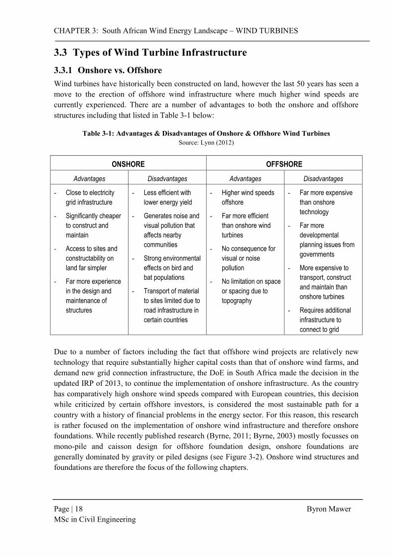
3.3 Types of Wind Turbine Infrastructure 3.3.1 Onshore vs. Offshore Wind turbines have historically been constructed on land, however the last 50 years has seen a move to the erection of offshore wind infrastructure where much higher wind speeds are currently experienced. There are a number of advantages to both the onshore and offshore structures including that listed in Table 3-1 below:
Table 3-1: Advantages & Disadvantages of Onshore & Offshore Wind Turbines Source: Lynn (2012)
ONSHORE OFFSHORE
Advantages Disadvantages Advantages Disadvantages
- Close to electricity
grid infrastructure
- Significantly cheaper
to construct and
maintain
- Access to sites and
constructability on
land far simpler
- Far more experience
in the design and
maintenance of
structures
- Less efficient with
lower energy yield
- Generates noise and
visual pollution that
affects nearby
communities
- Strong environmental
effects on bird and
bat populations
- Transport of material
to sites limited due to
road infrastructure in
certain countries
- Higher wind speeds
offshore
- Far more efficient
than onshore wind
turbines
- No consequence for
visual or noise
pollution
- No limitation on space
or spacing due to
topography
- Far more expensive
than onshore
technology
- Far more
developmental
planning issues from
governments
- More expensive to
transport, construct
and maintain than
onshore turbines
- Requires additional
infrastructure to
connect to grid
Due to a number of factors including the fact that offshore wind projects are relatively new technology that require substantially higher capital costs than that of onshore wind farms, and demand new grid connection infrastructure, the DoE in South Africa made the decision in the updated IRP of 2013, to continue the implementation of onshore infrastructure. As the country has comparatively high onshore wind speeds compared with European countries, this decision while criticized by certain offshore investors, is considered the most sustainable path for a country with a history of financial problems in the energy sector. For this reason, this research is rather focused on the implementation of onshore wind infrastructure and therefore onshore foundations. While recently published research (Byrne, 2011; Byrne, 2003) mostly focusses on mono-pile and caisson design for offshore foundation design, onshore foundations are generally dominated by gravity or piled designs (see Figure 3-2). Onshore wind structures and foundations are therefore the focus of the following chapters.
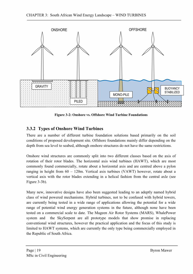
CHAPTER 3: South African Wind Energy Landscape – WIND TURBINES
Page | 19 Byron Mawer MSc in Civil Engineering
GRAVITY
PILED
MONO-PILE BUOYANCY STABILIZED
ONSHORE OFFSHORE
Figure 3-2: Onshore vs. Offshore Wind Turbine Foundations
3.3.2 Types of Onshore Wind Turbines There are a number of different turbine foundation solutions based primarily on the soil conditions of proposed development site. Offshore foundations mainly differ depending on the depth from sea level to seabed, although onshore structures do not have the same restrictions. Onshore wind structures are commonly split into two different classes based on the axis of rotation of their rotor blades. The horizontal axis wind turbines (HAWT), which are most commonly found commercially, rotate about a horizontal axis and are centred above a pylon ranging in height from 60 – 120m. Vertical axis turbines (VAWT) however, rotate about a vertical axis with the rotor blades extending in a helical fashion from the central axle (see Figure 3-3b). Many new, innovative designs have also been suggested leading to an adeptly named hybrid class of wind powered mechanisms. Hybrid turbines, not to be confused with hybrid towers, are currently being tested in a wide range of applications allowing the potential for a wide range of potential wind energy generation systems in the future, although none have been tested on a commercial scale to date. The Mageen Air Rotor Systems (MARS), WhalePower system and the SkySerpent are all prototype models that show promise in replacing conventional wind structures, however the practical application and the focus of this study is limited to HAWT systems, which are currently the only type being commercially employed in the Republic of South Africa.

CHAPTER 3: South African Wind Energy Landscape – WIND TURBINES
Page | 20 Byron Mawer MSc in Civil Engineering
Figure 3-3: Wind Turbine Structures by type - a) HAWT, b) VAWT, c) MARS Source: Lovett (2014); REUK (2014)
3.4 Horizontal Axis Wind Turbines 3.4.1 Structure The horizontal axis wind turbine is essentially divided into 3 main sections each with their own sub-sections. These parts, as shown in Figure 3-4 a), are the foundations, tower and the nacelle-rotor system. Each of these elements is extremely important as they both contribute significantly to the loading that is inherent on the structure.
Starting from the top of the structure, the nacelle houses all the mechanical and electrical equipment that facilitates the conversion of wind energy to rotational energy and finally to electrical energy. The process is rather simple; turbulent air in the form of wind passes over the rotor blades causing them to turn. The blades, which meet at the hub, are connected to a drivetrain, similar to an axle of a car. This drivetrain leads to a generator that generates the electricity. The nacelle also houses a gearbox as well as other devices that help control the pitch and speed of the rotor blades as they turn (Figure 3-4b)). This blade-hub-nacelle system is ultimately supported by the tower and all loads generated from this system are transferred to the foundations through the tower. The tower or pylon is often fabricated in interlocking steel sections, which are assembled on site and then slotted into the foundation base. The tower height can range between 30m to 130m onshore and can become even taller in offshore applications. Towers are typically transported to site in sections that are then assembled using a series of high lift capacity cranes. A more recent development has been the construction of concrete and hybrid towers that are assembled in the same way as for steel towers besides minor differences in the connection of each section (von der Haar, 2014). These designs are advantageous as transporting interlocking pre-cast elements can be far simpler than the large steel sections inherent of a purely steel tower (see Section 3.4.3).
a) b) c)
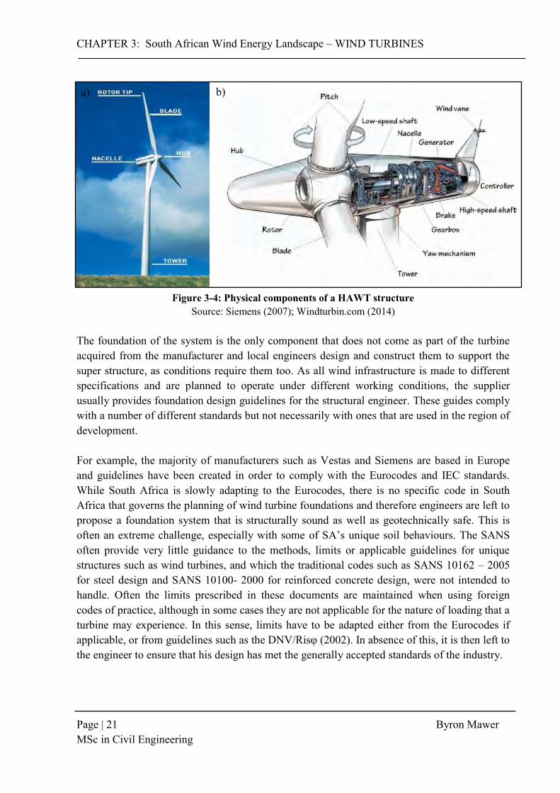
CHAPTER 3: South African Wind Energy Landscape – WIND TURBINES
Page | 21 Byron Mawer MSc in Civil Engineering
Figure 3-4: Physical components of a HAWT structure Source: Siemens (2007); Windturbin.com (2014)
The foundation of the system is the only component that does not come as part of the turbine acquired from the manufacturer and local engineers design and construct them to support the super structure, as conditions require them too. As all wind infrastructure is made to different specifications and are planned to operate under different working conditions, the supplier usually provides foundation design guidelines for the structural engineer. These guides comply with a number of different standards but not necessarily with ones that are used in the region of development. For example, the majority of manufacturers such as Vestas and Siemens are based in Europe and guidelines have been created in order to comply with the Eurocodes and IEC standards. While South Africa is slowly adapting to the Eurocodes, there is no specific code in South Africa that governs the planning of wind turbine foundations and therefore engineers are left to propose a foundation system that is structurally sound as well as geotechnically safe. This is often an extreme challenge, especially with some of SA’s unique soil behaviours. The SANS often provide very little guidance to the methods, limits or applicable guidelines for unique structures such as wind turbines, and which the traditional codes such as SANS 10162 – 2005 for steel design and SANS 10100- 2000 for reinforced concrete design, were not intended to handle. Often the limits prescribed in these documents are maintained when using foreign codes of practice, although in some cases they are not applicable for the nature of loading that a turbine may experience. In this sense, limits have to be adapted either from the Eurocodes if applicable, or from guidelines such as the DNV/Risφ (2002). In absence of this, it is then left to the engineer to ensure that his design has met the generally accepted standards of the industry.
a) b)
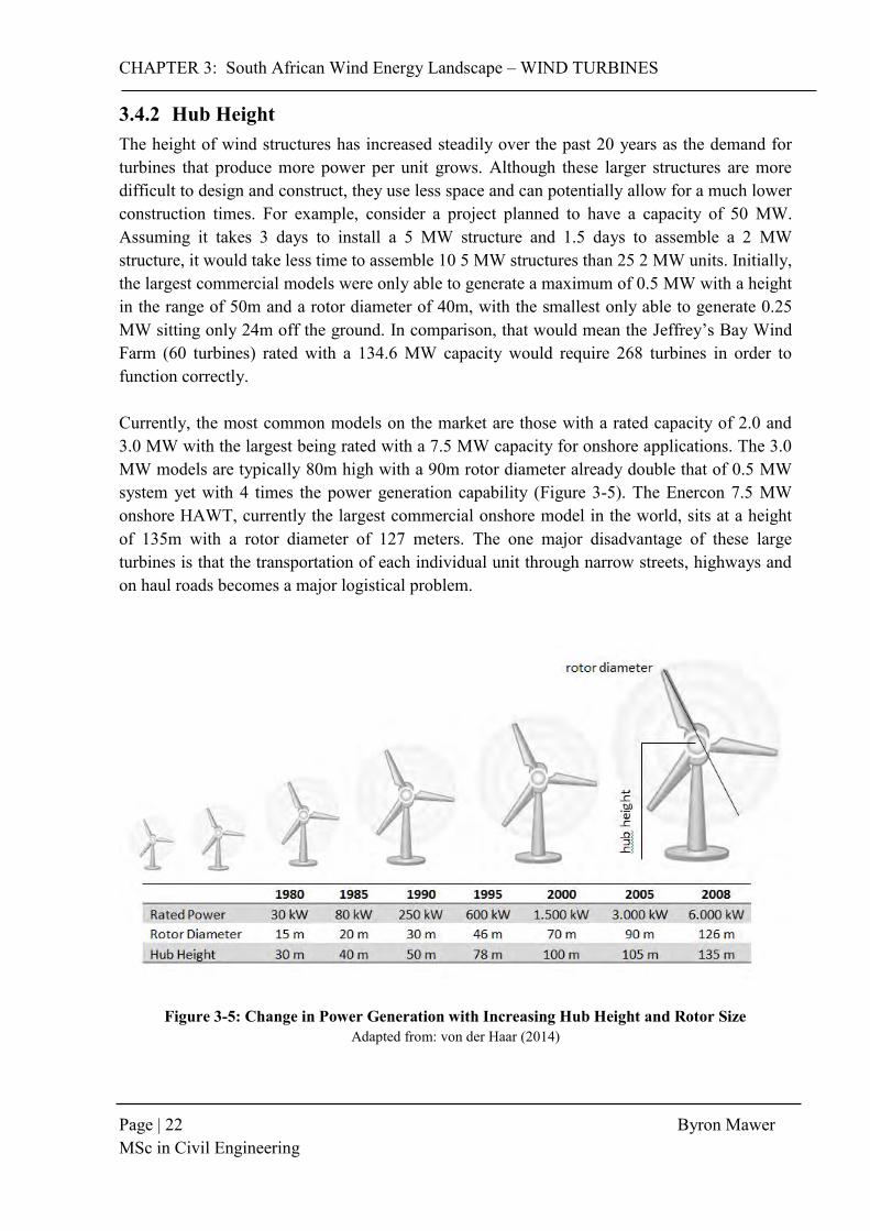
CHAPTER 3: South African Wind Energy Landscape – WIND TURBINES
Page | 22 Byron Mawer MSc in Civil Engineering
3.4.2 Hub Height The height of wind structures has increased steadily over the past 20 years as the demand for turbines that produce more power per unit grows. Although these larger structures are more difficult to design and construct, they use less space and can potentially allow for a much lower construction times. For example, consider a project planned to have a capacity of 50 MW. Assuming it takes 3 days to install a 5 MW structure and 1.5 days to assemble a 2 MW structure, it would take less time to assemble 10 5 MW structures than 25 2 MW units. Initially, the largest commercial models were only able to generate a maximum of 0.5 MW with a height in the range of 50m and a rotor diameter of 40m, with the smallest only able to generate 0.25 MW sitting only 24m off the ground. In comparison, that would mean the Jeffrey’s Bay Wind Farm (60 turbines) rated with a 134.6 MW capacity would require 268 turbines in order to function correctly. Currently, the most common models on the market are those with a rated capacity of 2.0 and 3.0 MW with the largest being rated with a 7.5 MW capacity for onshore applications. The 3.0 MW models are typically 80m high with a 90m rotor diameter already double that of 0.5 MW system yet with 4 times the power generation capability (Figure 3-5). The Enercon 7.5 MW onshore HAWT, currently the largest commercial onshore model in the world, sits at a height of 135m with a rotor diameter of 127 meters. The one major disadvantage of these large turbines is that the transportation of each individual unit through narrow streets, highways and on haul roads becomes a major logistical problem.
Figure 3-5: Change in Power Generation with Increasing Hub Height and Rotor Size Adapted from: von der Haar (2014)

CHAPTER 3: South African Wind Energy Landscape – WIND TURBINES
Page | 23 Byron Mawer MSc in Civil Engineering
3.4.3 Design Materials Historically, steel tubular structures have been the most commonly employed wind turbine commercially. However, as the height keeps increasing in order to take advantage of higher wind speeds at altitude, the size of wind energy infrastructure has been required to increase to meet the structural design requirements. With this growth in size, comes the use of larger amounts of steel, which as a construction material, is relatively expensive (TCC, 2007). This has led to a number of alternative tower designs including purely precast concrete towers, hybrid steel-concrete composite towers and reinforced concrete towers each with their own advantages and disadvantages depending on a number of factors including hub height, rotor diameter, material costs and comparative material benefits to state a few. The three main types of towers are discussed below:
3.4.3.1 Steel Towers Steel towers have historically been used due to their ease of manipulation and the material’s ability to handle a large range of tensile and compressive forces caused by the massive bending forces applied to the structure while being laterally loaded (Gaspar, 2012). This has resulted in the common tubular steel towers dominating the wind energy market over the past 20 years. Steel lattice towers have also been used in the past but never on the same scale as those of the tubular form. This is generally because they take significantly more space, however they do possess the advantage that they are subject to far less founding restrictions. Some of the largest turbines in the world have been built with a steel lattice support tower including the Fuhrlander system in Germany and the Nowy Tomysl turbine in Poland both standing 160m from the ground although they both only boast a capacity of 2.5MW. Accepting that steel towers have their limitations, they will continue to be the most commonly used across the world for units generating less than 5.0MW (Gaspar, 2012). According to Gaspar (2012), steel towers make up approximately 94% of all commercial wind energy infrastructure across the world. While this trend is expected to decrease slightly, steel tubular towers will still form the majority of new installed towers for the foreseeable future. This is due to their saturation in the market and the fact that their steel structural models have been perfected over the last decade which has led to economic and trusted designs for engineers and investors. While there are some companies in South Africa and Europe that have begun to produce precast concrete units, most commercial wind turbines currently consist of typical steel tubular towers produced by one of the major manufacturers such as Vestas or Siemens. For towers that are required to generate more than 5.0 MW, concrete and hybrid towers are becoming more beneficial for investors. There are a number of reasons for this including the logistical problem of transporting massive 4.5m diameter sections of the steel tower to site, which in South Africa particularly, can be up to 600km from the nearest port. The railway network in SA is also not favoured due to a number of factors and therefore steel tower sections are trucked to site. This is one of the key reasons why access and haul roads are a vital
CHAPTER 3: South African Wind Energy Landscape – WIND TURBINES
Page | 24 Byron Mawer MSc in Civil Engineering
part of any design for a wind energy project (Day, 2014). The other notable disadvantage of steel tower turbines is the volatility in steel price compared to concrete in the past 30 years. For long term contracts, investors and contractors open themselves up to the risk of losing large amounts of their profit due to fluctuating steel prices and the consequent increase in cost of purchasing the units from the supplier. While this can be avoided with proper planning, concrete offers an alternative that does not suffer from the same ailment.
3.4.3.2 Hybrid Towers There are a number of different concrete hybrid towers that can be used when constructing a turbine, each with a different construction method, which can be specifically selected depending on the capability of the contractor. The advantages of hybrid towers are that they can be more economical due to the lower volumes of steel required in their designs. They can also be built to great heights without being limited by the tensile strength of reinforced concrete. Another major advantage is that the transport of the large base sections is simpler for precast concrete segments than that of steel, making it extremely advantageous for projects in remote locations. The main types of hybrid tower that are found in the European market include the following:
- ENERCON Design: The hybrid ENERCON design combines the trusted concrete tower construction method (Figure 3-6) which includes a number of concrete segments internally post-tensioned combined with a small tubular steel component for the top third of the turbine tower reach. Vertical joints are reinforced concrete combined with additional longitudinal reinforcement to ensure structural integrity of the connections. Horizontal joints are connected with an epoxy polymer to limit any movement during extreme loading conditions.
- Max Bőgl Design: The Max Bőgl design very closely follows that of the ENERCON hybrid tower. The main difference being that: half the tower consists of tubular precast concrete sections with external post-tensioning combined with tubular steel sections at the upper reaches of the turbine. Vertical joints are reinforced with mortar and concrete while the horizontal joints are unique in the sense that they rely purely on friction with no concrete or epoxy to secure the connection. This construction method has won numerous awards in Europe due to its innovative nature and reliable results.
- Advanced Tower System (ATS): The ATS is a hybrid reinforced concrete design that makes use of a quadratic tower shape in order to maximize longitudinal stiffness to heights of 120m. It consists of several precast segments that are joined vertically with a reinforced concrete joint and horizontally with a bolted joint sealed with mortar or epoxy depending on the design. Some versions of this method also incorporate a steel shell or steel sections depending on local conditions. A number of these systems have been employed in Europe such as at the Salbatica II wind farm in Romania.
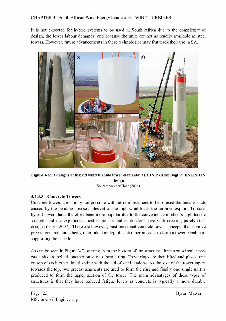
CHAPTER 3: South African Wind Energy Landscape – WIND TURBINES
Page | 25 Byron Mawer MSc in Civil Engineering
It is not expected for hybrid systems to be used in South Africa due to the complexity of design, the lower labour demands, and because the units are not as readily available as steel towers. However, future advancements in these technologies may fast track their use in SA.
Figure 3-6: 3 designs of hybrid wind turbine tower elements: a) ATS, b) Max Bőgl, c) ENERCON
design Source: van der Haar (2014)
3.4.3.3 Concrete Towers Concrete towers are simply not possible without reinforcement to help resist the tensile loads caused by the bending stresses inherent of the high wind loads the turbines exploit. To date, hybrid towers have therefore been more popular due to the convenience of steel’s high tensile strength and the experience most engineers and contractors have with erecting purely steel designs (TCC, 2007). There are however, post-tensioned concrete tower concepts that involve precast concrete units being interlinked on top of each other in order to form a tower capable of supporting the nacelle. As can be seen in Figure 3-7, starting from the bottom of the structure, three semi-circular pre-cast units are bolted together on site to form a ring. These rings are then lifted and placed one on top of each other, interlocking with the aid of steel tendons. As the size of the tower tapers towards the top, two precast segments are used to form the ring and finally one single unit is produced to form the upper section of the tower. The main advantages of these types of structures is that they have reduced fatigue levels as concrete is typically a more durable
a) b) c)
c)
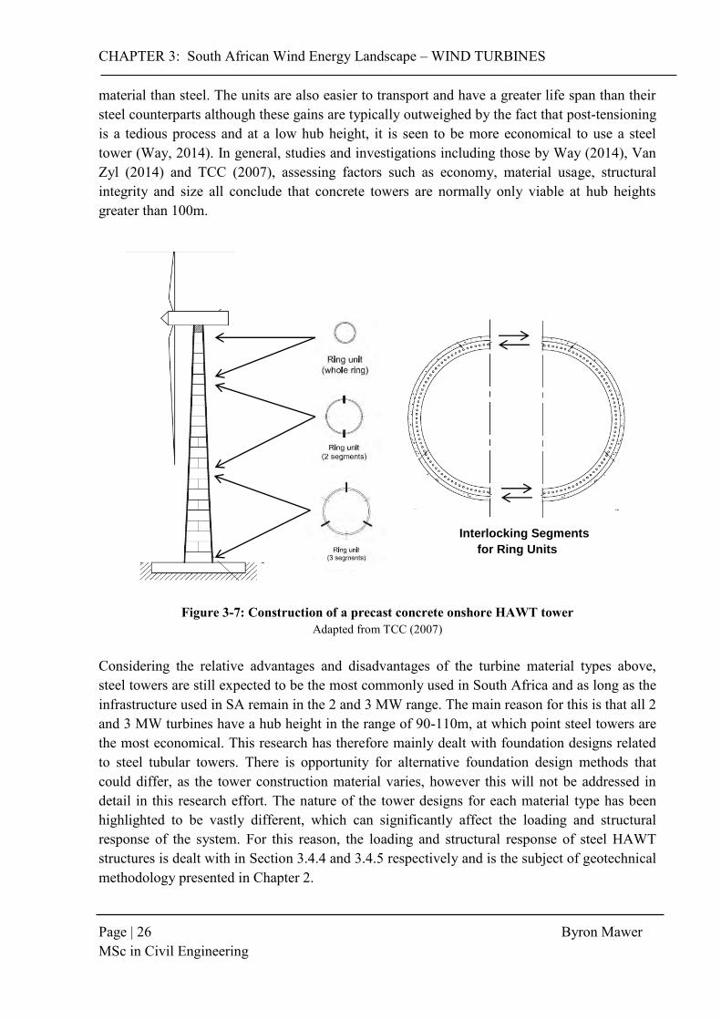
CHAPTER 3: South African Wind Energy Landscape – WIND TURBINES
Page | 26 Byron Mawer MSc in Civil Engineering
material than steel. The units are also easier to transport and have a greater life span than their steel counterparts although these gains are typically outweighed by the fact that post-tensioning is a tedious process and at a low hub height, it is seen to be more economical to use a steel tower (Way, 2014). In general, studies and investigations including those by Way (2014), Van Zyl (2014) and TCC (2007), assessing factors such as economy, material usage, structural integrity and size all conclude that concrete towers are normally only viable at hub heights greater than 100m.
Figure 3-7: Construction of a precast concrete onshore HAWT tower
Adapted from TCC (2007) Considering the relative advantages and disadvantages of the turbine material types above, steel towers are still expected to be the most commonly used in South Africa and as long as the infrastructure used in SA remain in the 2 and 3 MW range. The main reason for this is that all 2 and 3 MW turbines have a hub height in the range of 90-110m, at which point steel towers are the most economical. This research has therefore mainly dealt with foundation designs related to steel tubular towers. There is opportunity for alternative foundation design methods that could differ, as the tower construction material varies, however this will not be addressed in detail in this research effort. The nature of the tower designs for each material type has been highlighted to be vastly different, which can significantly affect the loading and structural response of the system. For this reason, the loading and structural response of steel HAWT structures is dealt with in Section 3.4.4 and 3.4.5 respectively and is the subject of geotechnical methodology presented in Chapter 2.
Interlocking Segments
for Ring Units
CHAPTER 3: South African Wind Energy Landscape – WIND TURBINES
Page | 27 Byron Mawer MSc in Civil Engineering
3.5 Loading Wind turbines experience a number of different static and dynamic loads, including gravitational, inertial and aerodynamic forces. While particular loading considerations are discussed in the design methodology (Section 4.6), it is important to understand that wind infrastructure has a number of operational states, which cause different loads to be applied to the structure at any point in its lifetime. This is mainly due to the ability of wind turbine controllers being able to change the speed of rotation of the system as well as the angle of attack of the rotor blades into the flowing air column in order to improve efficiency. To fully understand the design of the structure’s foundations, the mechanics, operational states and controlling mechanisms need to be addressed.
3.5.1 Wind Turbine Aerodynamics The efficiency and power generating capacity of a turbine is directly related to the airflow that is causing the rotation of the rotor blades. In order to understand the forces that are transferred to the foundations, it is important to first consider the complex interactions between the air columns moving past the turbine blades. The rotation of the blades is dictated by two main forces caused by the interaction of the flowing air and the blades themselves. These forces are drag and lift, common terms used in aeronautics. Lift as described in aeronautics, is the force acting at right angles to an object, in response to a disturbance caused in the moving fluid in which it is placed. The name originates from aircraft wing design, where this force makes the plane tend to lift up. In contrast, Drag is the force experienced by an object in response to the disturbance caused in a moving fluid, acting parallel to the fluids movement, and normally attempts to resist an objects motion through the fluid itself. The net force acting on the object is then the vector sum of both the drag and lift forces plus any other forces that may be acting on the object such as a thrust caused by the engines of an aircraft for example. Lynn (2012) describes this by making use of the following example: Figure 3-8 shows a flat plate with air moving from left to right. In a), the plate is orientated in the same direction as that of the airflow. Assuming there is no friction, the plate creates no disturbance in the airflow and therefore no drag or lift is experienced. In b), the plate is angled at an angle α into the direction of the fluids motion. The drag forces generated try to resist or push the object away from the fluids motion, while a lift force attempts to move the object at right angles to the airs motion. Finally, in c) with the plate orientated at 90° to the flow of the air column, no lift can be generated and therefore only drag forces are experienced by the plate. With this orientation, the max drag force is experienced if turbulent effects of fluid flow are ignored.

CHAPTER 3: South African Wind Energy Landscape – WIND TURBINES
Page | 28 Byron Mawer MSc in Civil Engineering
Figure 3-8: Drag and Lift forces on a plate placed in fluid flow Source: Lynn (2012)
With an aircraft, this lift force is used to balance the weight of the airplane and sometimes even exceed it such as during take-off, while drag is minimized so that the engine providing the thrust does not have to be worked harder than necessary. Conversely, during the landing of an aircraft, lift must be reduced while drag must increase in order help slow the airplane to a stop (see Figure 3-9). The wings of an aircraft, similarly to the blades of wind turbine are designed to maximize and minimize these forces accordingly by changing the angle at which they are orientated into the direction of the fluid’s direction of flow. This angle is often referred to as the angle of attack and is measured between the chord - the length from centre to centre of the leading edge of the wing or blade and the trailing edge – and the direction of the fluids motion.
Figure 3-9: Principles of drag and lift as it applies to aircraft wings
Adapted from: Lynn (2012) Another important phenomenon concerning objects subject to the effects of fluid flow, is the idea of stall. In aircraft, when a plane is travelling at low speed and the angle of attack is too high, there is a very sudden drop in lift and increase in drag, which can causes the aircraft to begin to fall out the sky. This is important according to Bonnet, (2005) and Lynn, (2012) as stalling can be actively used to control the power generation capability of turbines especially when the wind speeds get high enough that it might damage the generators that produce
lift
drag
drag
a) b) c)

CHAPTER 3: South African Wind Energy Landscape – WIND TURBINES
Page | 29 Byron Mawer MSc in Civil Engineering
electricity. With the ideas of lift, drag and stall explained, the theory can now be applied to wind turbine blades so that the forces during the various operational states can be understood. As aircraft make use of lift to balance out the weight of the body of the vehicle, horizontal wind turbines make use of lift to generate a rotation around the horizontal axis of the turbine. Vertical axis wind turbines can also make use of lift to generate rotation around the vertical axis however; the majority of vertical turbines actually make use of drag. The problem with drag driven wind turbines is that the speed of the turbine will be limited by the average wind speed that prevails in the location where the turbine is placed, as drag relies on getting as much surface area into the wind as possible. The advantage of modern HAWT structures is that they make use of lift to drive the rotor, and in contrast to drag driven systems, this is not limited by wind speed, which results in HAWT’s being able to generate wind speeds far higher than that of the prevailing wind speed in the area (Lynn, 2012). In order to understand the mechanics behind the rotation of a turbine, Lynn (2012) considers a typical lift driven HAWT as shown in Figure 3-10, the wind direction is shown from left to right with a section of a turbine rotor blade in its relative position to the hub. If compared to Figure 3-9, it becomes evident that the blade on the turbine is equivalent to the aircraft wing from Figure 3-9 placed with its underside directly facing the oncoming wind. This may seem confusing as, by the previous discussion, this would mean the rotor would produce significant drag and very little lift. However, the key distinction between the aerodynamics of a plane wing and that of a wind turbine is that as a turbine blade rotates, it creates its own wind orthogonal to the natural prevailing wind. It is the vector combination of both the natural and generated wind that produces the resultant pressure that turbine blades are designed for. The generated wind is often dominant as it increases dramatically the further you move out from the hub with its speed calculated using Equation 2: 𝑣 = 𝛺. 𝑟 (Eqn 2) Where v = generated wind speed (m/s) Ω = angular velocity of rotor blades (rad/s) r = the distance from the center of the hub (m) With modern turbines having blade lengths of up to 100m for a 5 MW turbine, the generated wind speed can be extremely high and significantly greater than that of the prevailing natural airflow speed. As this equation shows how the wind speed will increase as you move further out from the hub, it can be expected that the resultant winds angle of attack on the blade will constantly be changing, as the resultant force becomes more and more influenced by the generated wind from the turbine. The angle of attack therefore must change in order to maximize lift. This is the reason that modern turbine blades have the appearance of being twisted as they move out from the hub.

CHAPTER 3: South African Wind Energy Landscape – WIND TURBINES
Page | 30 Byron Mawer MSc in Civil Engineering
Figure 3-10: Aerodynamic principles behind operation of a HAWT Source: Lynn (2012)
With the resultant aerodynamic force now acting at some vertical angle up towards the centre of the hub, the generated forces can now be shown as represented by (4), (5) and (6) in Figure 3-10. (4) represents the lift generated from the resultant wind, (5) the drag and (6) the resultant of the vector combination of these two aerodynamic forces. Critically, this resultant force can be resolved into a horizontal and vertical component as shown above. The vertical portion of the resultant (7) is the component that causes the rotor to rotate and generate power. The horizontal component (8) is the one that causes stress in the rotor blades by attempting to bend them backwards. It then follows that blade designers would wish to maximize the radial force and minimize the horizontal component that acts on the turbine. This, Lynn (2012) explains, is why ensuring the blades of the structure are orientated at the right angle of attack is so critical, as the higher the drag, the greater the horizontal component of the resultant aerodynamic force will be. With this understanding, the different operation modes of a wind turbine, which are primarily based on enforcing different states of stall in the system, can now be investigated. This ultimately will aid in the comprehension of the loading information provided in the design methodology.
(1) Natural Prevailing Wind
(2) Turbine Generated Wind
(3) Resultant Wind
(4) Lift Force
(5) Drag Force
(6) Resultant Aerodynamic Force
(7) Horizontal Component of Resultant
(8) Vertical Component of Resultant
CHAPTER 3: South African Wind Energy Landscape – WIND TURBINES
Page | 31 Byron Mawer MSc in Civil Engineering
3.5.2 Operational States Wind turbines have a number of operational states, each that have a different effect on loading, and this needs to be accounted for by an engineer when conducting the structural or foundation design. The operational states according to Warren-Codrington (2013) drawn from IEC 61400-1 and DNV/Risφ (2002) include: 1) Parked, 2) Normal Operation, 3) Start-up & Shut down, 4) Normal Operation under extreme environmental conditions, and 5) Abnormal or Fault States The parked state is one in which the rotor’s rotation is restricted with no movement being possible even in high winds. A simple analogy for this would be a car with its handbrake engaged. Most wind turbines are placed in a parked state when environmental conditions are considered too extreme for operation and therefore a critical design option for the most severe loading at ULS is often when the turbine is parked. The normal operation state is when a turbine is active and rotating at lower than, or at design speed. Control measures can be put in place to allow a turbine to function at above design speed but this will be discussed later in this section. According to IEC 61400-1, due to the fact that a turbine will spend most of its design life in the normal operation state, the ULS, SLS and fatigue limit states must be checked for a turbine at its design speed, and higher if making use of speed control systems. If there are extreme weather conditions such as unusually strong gusts, ice and snow or even large wave action for offshore turbines, these must all be taken into account for the parked and normal operation operational states in design. The start-up and shut-down operation states take into account the force applied by the rotor brakes and the shutdown or start-up of the machinery housed in the nacelle. Normally these forces do not exceed those of the parked or normal operation ULS cases (Vestas, 2013) however, due to the change in vibrations of the machinery and frequencies of rotation of the rotor blades, there may be a point where the natural frequency of the tower is reached causing amplified deflections or stresses. For this reason, this can be an important case to consider during the structural design. Finally, an abnormal fault state can exist when there is a mechanical problem with the turbine and it is not operating correctly. A typical fault such as a brake failure or a gearbox failure can allow the turbine to spin faster than it should which needs to be accounted for. Different load factors and applied loads are applicable for each operation state and are dealt with as separate load cases in design. These cases are generally considered only by the manufacturer and these operating states do not affect the foundation design unless otherwise stated.

CHAPTER 3: South African Wind Energy Landscape – WIND TURBINES
Page | 32 Byron Mawer MSc in Civil Engineering
3.5.3 Control Measures To regulate the power production of wind turbine generators, a number of control measures are built into modern rotor blade design, which in turn can have an effect on the structural actions experienced in each of the loading cases discussed in the previous section. These control measures are put in place by either managing the pitch of the blades or making use of the phenomenon of stall to limit production in extreme conditions. One of the following philosophies is adopted depending on the external conditions as well as the level of control desired by the controller: 1) Active Stall Regulation (shown in Figure 3-11a), 2) Passive Stall Regulation (shown in Figure 3-11b), and 3) Pitch Regulation (shown in Figure 3-11c).
Figure 3-11: Blade behavior under power control measures (a) active stall, (b) passive stall and (c)
pitch controlled. Source: Bonnet (2005); Warren-Codrington (2013)
a) b) c)
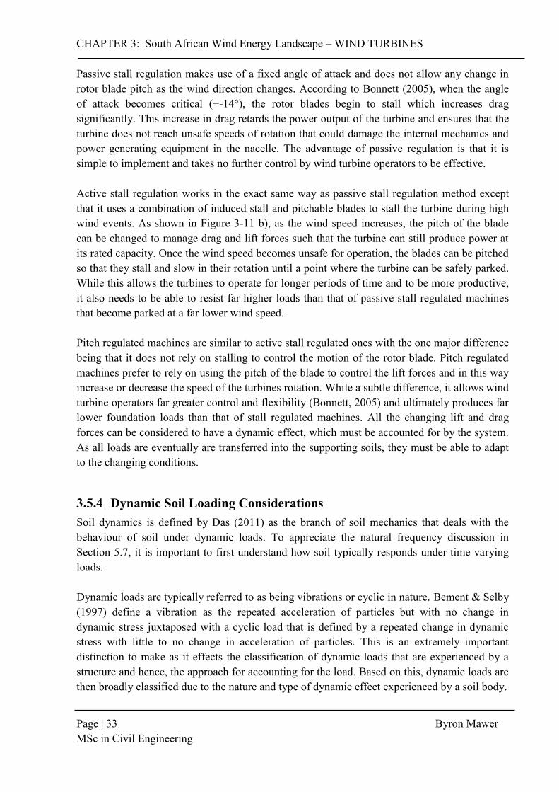
CHAPTER 3: South African Wind Energy Landscape – WIND TURBINES
Page | 33 Byron Mawer MSc in Civil Engineering
Passive stall regulation makes use of a fixed angle of attack and does not allow any change in rotor blade pitch as the wind direction changes. According to Bonnett (2005), when the angle of attack becomes critical (+-14°), the rotor blades begin to stall which increases drag significantly. This increase in drag retards the power output of the turbine and ensures that the turbine does not reach unsafe speeds of rotation that could damage the internal mechanics and power generating equipment in the nacelle. The advantage of passive regulation is that it is simple to implement and takes no further control by wind turbine operators to be effective. Active stall regulation works in the exact same way as passive stall regulation method except that it uses a combination of induced stall and pitchable blades to stall the turbine during high wind events. As shown in Figure 3-11 b), as the wind speed increases, the pitch of the blade can be changed to manage drag and lift forces such that the turbine can still produce power at its rated capacity. Once the wind speed becomes unsafe for operation, the blades can be pitched so that they stall and slow in their rotation until a point where the turbine can be safely parked. While this allows the turbines to operate for longer periods of time and to be more productive, it also needs to be able to resist far higher loads than that of passive stall regulated machines that become parked at a far lower wind speed. Pitch regulated machines are similar to active stall regulated ones with the one major difference being that it does not rely on stalling to control the motion of the rotor blade. Pitch regulated machines prefer to rely on using the pitch of the blade to control the lift forces and in this way increase or decrease the speed of the turbines rotation. While a subtle difference, it allows wind turbine operators far greater control and flexibility (Bonnett, 2005) and ultimately produces far lower foundation loads than that of stall regulated machines. All the changing lift and drag forces can be considered to have a dynamic effect, which must be accounted for by the system. As all loads are eventually are transferred into the supporting soils, they must be able to adapt to the changing conditions.
3.5.4 Dynamic Soil Loading Considerations Soil dynamics is defined by Das (2011) as the branch of soil mechanics that deals with the behaviour of soil under dynamic loads. To appreciate the natural frequency discussion in Section 5.7, it is important to first understand how soil typically responds under time varying loads. Dynamic loads are typically referred to as being vibrations or cyclic in nature. Bement & Selby (1997) define a vibration as the repeated acceleration of particles but with no change in dynamic stress juxtaposed with a cyclic load that is defined by a repeated change in dynamic stress with little to no change in acceleration of particles. This is an extremely important distinction to make as it effects the classification of dynamic loads that are experienced by a structure and hence, the approach for accounting for the load. Based on this, dynamic loads are then broadly classified due to the nature and type of dynamic effect experienced by a soil body.
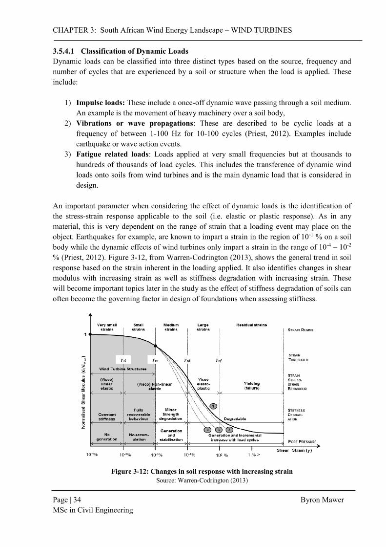
CHAPTER 3: South African Wind Energy Landscape – WIND TURBINES
Page | 34 Byron Mawer MSc in Civil Engineering
3.5.4.1 Classification of Dynamic Loads Dynamic loads can be classified into three distinct types based on the source, frequency and number of cycles that are experienced by a soil or structure when the load is applied. These include:
1) Impulse loads: These include a once-off dynamic wave passing through a soil medium. An example is the movement of heavy machinery over a soil body,
2) Vibrations or wave propagations: These are described to be cyclic loads at a frequency of between 1-100 Hz for 10-100 cycles (Priest, 2012). Examples include earthquake or wave action events.
3) Fatigue related loads: Loads applied at very small frequencies but at thousands to hundreds of thousands of load cycles. This includes the transference of dynamic wind loads onto soils from wind turbines and is the main dynamic load that is considered in design.
An important parameter when considering the effect of dynamic loads is the identification of the stress-strain response applicable to the soil (i.e. elastic or plastic response). As in any material, this is very dependent on the range of strain that a loading event may place on the object. Earthquakes for example, are known to impart a strain in the region of 10-1 % on a soil body while the dynamic effects of wind turbines only impart a strain in the range of 10-4 – 10-2 % (Priest, 2012). Figure 3-12, from Warren-Codrington (2013), shows the general trend in soil response based on the strain inherent in the loading applied. It also identifies changes in shear modulus with increasing strain as well as stiffness degradation with increasing strain. These will become important topics later in the study as the effect of stiffness degradation of soils can often become the governing factor in design of foundations when assessing stiffness.
Figure 3-12: Changes in soil response with increasing strain Source: Warren-Codrington (2013)

CHAPTER 3: South African Wind Energy Landscape – WIND TURBINES
Page | 35 Byron Mawer MSc in Civil Engineering
3.5.4.2 Dynamic Soil Behaviour When analysing any materials behaviour under loading, it is always important to analyse the stress-strain relationship that is exhibited as this, more often than not, governs a materials behaviour under loading (Karg, 2008). In soils, it is essential to analyse the relationship between shear stress and strain as the majority of soils will fail by some mechanism that is related to shear strains (Das & Ramana, 2011). Soils under the influence of cyclic loading, particularly with loads causing strain rates of between 10-4 and 10-2 %, tend to show elastoplastic behaviour. In practical terms, this means that the shear modulus (modulus that relates shear stress to shear strain) decreases as the strain on the soil increases. In addition to this, Priest (2012) describes that energy is dissipated during each stress cycle due to particle slippage at each of the grain contact points. This energy loss is referred to as damping, and is hysteretic in nature. This relationship is shown visually in Figure 3-13 below and is often referred to as the hysteretic loop in literature. For wind turbine structures the strain range is generally assumed to fall within the elastic behaviour range, however with fatigue over thousands of cycles, the stiffness of the soil can degrade to a point where elastoplastic behaviour may be experienced. In this case, the analysis of the dynamic soil response is important for design. To account for this, the dynamic soil properties must be sourced from the stress-strain relationship found in each soils unique hysteric loop.
Figure 3-13: Hysteretic loop of shear stress-strain relationship for soils under dynamic loading Source: Priest (2012)
1) 2)

CHAPTER 3: South African Wind Energy Landscape – WIND TURBINES
Page | 36 Byron Mawer MSc in Civil Engineering
The shear stress vs. strain graph in Figure 3-13 can essentially be considered as two curves: 1) Monotonic loading curve (often referred to as backbone curve), and 2) Hysteretic loop. The hysteric curve is commonly drawn by making use of laboratory soils tests such as cyclic triaxial or resonant column tests. The gradients of the measured response are equivalent to the shear modulus of the soil being investigated. The initial gradient of the backbone curve is equivalent to Gmax (the shear modulus at very small strains) while G (the secant modulus) is given by Equation 3:
𝐺 = 𝜏𝑎
𝛾𝑎 (Eqn 3)
Where: G = Secant modulus;
τa = Shear stress at a specific strain; 𝛾𝑎 = Shear strain at a specific stress
The G value is typically calculated in design making use of a stiffness reduction curve that calculates the secant modulus based on the level of strain that is expected in the soil due to the structural loading being transmitted to it. A number of stiffness degradation curves are available to a geotechnical designer and have been studied in some detail by Archer (2014). Table 3-2 below, quoted from his research, gives a number of theoretical stiffness degradation curves that could be used for design, each having been developed for a particular soil type or loading situation. Using the suggestions made by Clayton & Heymann (2001), the stiffness reduction curve proposed last in Table 3-2 above was used during this research. Other reduction curves should give representative results for SA soils if the material constants are appropriately obtained for the soil being investigated. The damping phenomenon in a soil can also be quantified from the hysteretic stress-strain relationship by relating the diagram to the energy dissipated through a loading cycle. The phenomenon is often reported by the Damping Ratio (ϛ) which is given by Equation 4:
ϛ = 1
4𝜋
∆𝑊
𝑊 (Eqn 4)
Where: ϛ = damping ratio for the soil ΔW = energy loss per cycle W = total stored energy (area under stress-strain curve)

CHAPTER 3: South African Wind Energy Landscape – WIND TURBINES
Page | 37 Byron Mawer MSc in Civil Engineering
Table 3-2: Stiffness degradation curves for calculation of secant shear modulus G Source: Archer (2014)
EQUATION REFERENCE NO. OF
VARIABLES
𝐸
𝐸0=
𝐺
𝐺0=
1
1 + 𝛼𝑅𝑦𝑅−1
- α, R are soil parameters based on the level of strain in the soil,
- E, G is the reduced Young’s modulus and shear strain,
- E0, G0 is the small strain Young’s modulus and shear strain
- 𝑦 = 𝑟⁄
1+ 𝑟⁄
- ε is axial strain at current stress level
- εr is the reference strain (𝑞𝑚𝑎𝑥 𝐸0)⁄
Ramberg & Osgood
(1943) 4
𝐸
𝐸0=
𝐺
𝐺0=
1
1 + 𝛾ℎ
With:
𝛾ℎ =𝛾
𝛾𝑟[1 + 𝑎. 𝑒
−𝑏(𝛾𝛾𝑟
)]
Where:
- α, b are soil parameters based on the level of strain in the soil,
- E, G is the reduced Young’s modulus and shear strain,
- E0, G0 is the small strain Young’s modulus and shear strain
- γ is the current strain in the soil
- γr is the reference strain (𝑞𝑚𝑎𝑥 𝐸0)⁄
- γh is the hyperbolic strain in the soil
Hardin & Dnervich
(1972) 4
𝐸
𝐸0=
𝐺
𝐺0= (1 − (
∆𝑞
𝑞𝑚𝑎𝑥)
𝑚
)𝑛
Where:
- E, G is the reduced Young’s modulus and shear strain,
- E0, G0 is the small strain Young’s modulus and shear strain
- Δq is the deviator stress
- qmax is max applied pressure
- m,n are material constants
Shibuya et al. (1997) 3
𝐺
𝐺0=
𝐸
𝐸0=
1
[1 + 16𝛾(1 + 10−20𝛾)]
Where:
- E, G is the reduced Young’s modulus and shear strain,
- E0, G0 is the small strain Young’s modulus and shear strain
- γ is the level of strain in the soil
Clayton & Heymann
(2001) 1
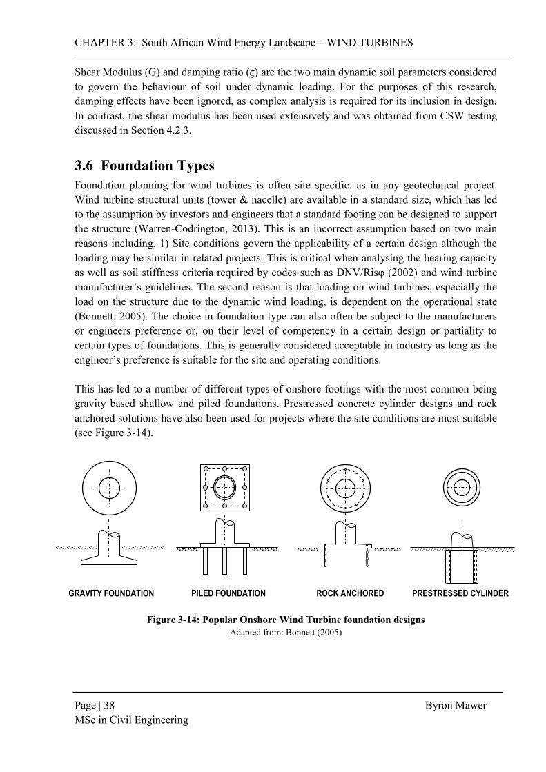
CHAPTER 3: South African Wind Energy Landscape – WIND TURBINES
Page | 38 Byron Mawer MSc in Civil Engineering
Shear Modulus (G) and damping ratio (ϛ) are the two main dynamic soil parameters considered to govern the behaviour of soil under dynamic loading. For the purposes of this research, damping effects have been ignored, as complex analysis is required for its inclusion in design. In contrast, the shear modulus has been used extensively and was obtained from CSW testing discussed in Section 4.2.3.
3.6 Foundation Types Foundation planning for wind turbines is often site specific, as in any geotechnical project. Wind turbine structural units (tower & nacelle) are available in a standard size, which has led to the assumption by investors and engineers that a standard footing can be designed to support the structure (Warren-Codrington, 2013). This is an incorrect assumption based on two main reasons including, 1) Site conditions govern the applicability of a certain design although the loading may be similar in related projects. This is critical when analysing the bearing capacity as well as soil stiffness criteria required by codes such as DNV/Risφ (2002) and wind turbine manufacturer’s guidelines. The second reason is that loading on wind turbines, especially the load on the structure due to the dynamic wind loading, is dependent on the operational state (Bonnett, 2005). The choice in foundation type can also often be subject to the manufacturers or engineers preference or, on their level of competency in a certain design or partiality to certain types of foundations. This is generally considered acceptable in industry as long as the engineer’s preference is suitable for the site and operating conditions. This has led to a number of different types of onshore footings with the most common being gravity based shallow and piled foundations. Prestressed concrete cylinder designs and rock anchored solutions have also been used for projects where the site conditions are most suitable (see Figure 3-14).
Figure 3-14: Popular Onshore Wind Turbine foundation designs Adapted from: Bonnett (2005)
GRAVITY FOUNDATION PILED FOUNDATION ROCK ANCHORED PRESTRESSED CYLINDER
CHAPTER 3: South African Wind Energy Landscape – WIND TURBINES
Page | 39 Byron Mawer MSc in Civil Engineering
3.6.1 Gravity Foundations A gravity foundation is typically considered a very large, wide and heavy shallow footing that relies on its high mass to resist the large moment loads applied to the structure. The gravity foundation has been the most widely used footing type for wind infrastructure around the world where site conditions allow for their use (Morgan, 2008). The designs often consist of either circular or rectangular geometries that have breadths or diameters of between 15-30m. They are constructed in-situ using reinforced concrete with an insertable steel cage in the centre used for the attachment of the tower. These types of footings are generally suited to soils which have uniform properties across the length of the base and have shear strength parameters that lead to medium to high bearing capacities and soil stiffness’s, with the water tables occurring far below the foundation base. Due to the large area of contact between the foundation and the soil, high water pressures below the base can cause large uplift forces that destabilize these types of footings making them unsuitable. In South Africa, where the country is one of the driest in the world, with an average annual rainfall of approximately 450mm - compared to the world average of 860mm (SA Info, 2015) - gravity foundations are generally viable options for design.
3.6.2 Piled Foundations Pile foundations, taking the form of long slender columns driven or bored and cast-in-situ, are used when soil conditions close to the surface are inadequate to support the structure. Piles transmit loading from the turbine to the subgrade through friction, end bearing or a combination of both. High lateral resistances are also required in order to resist the lateral earth pressures applied to the pile as well as the large bending moments conveyed from the structure. Generally, a series of between 6 to 24 piles are used depending on size, length and material type of the pile. Piles are then grouped using a cap which is significantly smaller than size of a gravity footing. Pile designs have been used in projects across the globe including SA when sub-surface soil conditions have been poor or there has been a threat of uplift from groundwater however, the planning and construction methods required for piles are often complex and expensive in comparison with the gravity foundation alternatives.
3.6.3 Caissons & Prestressed Cylinder Design A caisson or prestressed cylinder type foundation could be viewed as a combination between the gravity and pile designs. Essentially, caissons are large either circular, rectangular or polygonal hollow piles that are sunk into the ground to a depth where the structure can safely be founded. Caissons are often used in South Africa for bridge abutments and foundations, as they are well suited to dealing with the effects of a perched water table (Byrne & Berry, 2008).

CHAPTER 3: South African Wind Energy Landscape – WIND TURBINES
Page | 40 Byron Mawer MSc in Civil Engineering
They are very common for founding offshore wind energy infrastructure but less so for the onshore variation due to the relative merits of gravity or pile designs. The major reason for the lack of use of caissons onshore is due to the lack of expertise in caisson design and the fact that very strict monitoring of the installation is required in order for the caisson to generate the required bearing resistance. It has been advised to the DoE that these foundations only be investigated further for offshore applications or for areas where ground water is close to the surface in the South African market.
3.6.4 Rock Anchored Rock anchored foundations consist of a base foundation cap, similar to a pile cap or raft foundation that is anchored to bedrock. This type of foundation is only applicable to soil conditions where bedrock is reachable at shallow depths. Anchors are generally grouted into boreholes and post-tensioned in order to resist overturning and high moment loads. These types of founding solutions are generally limited by the compressive strength of the base cap as the bedrock can often have far higher compressive strengths than that of 30 MPa. While the use and design of rock anchor systems is well understood and widely used in South Africa, they are typically used in slope stability and retaining wall reinforcement applications and not in foundation designs. Even when rock anchored solutions may be more economical, the time it would take to design and the willingness of an engineer to take on an unfamiliar founding method generally makes the gravity foundation more attractive for investors.

PART II
GEOTECHNICAL DESIGN METHODOLOGY FOR
SOUTH AFRICAN SOIL CONDITIONS
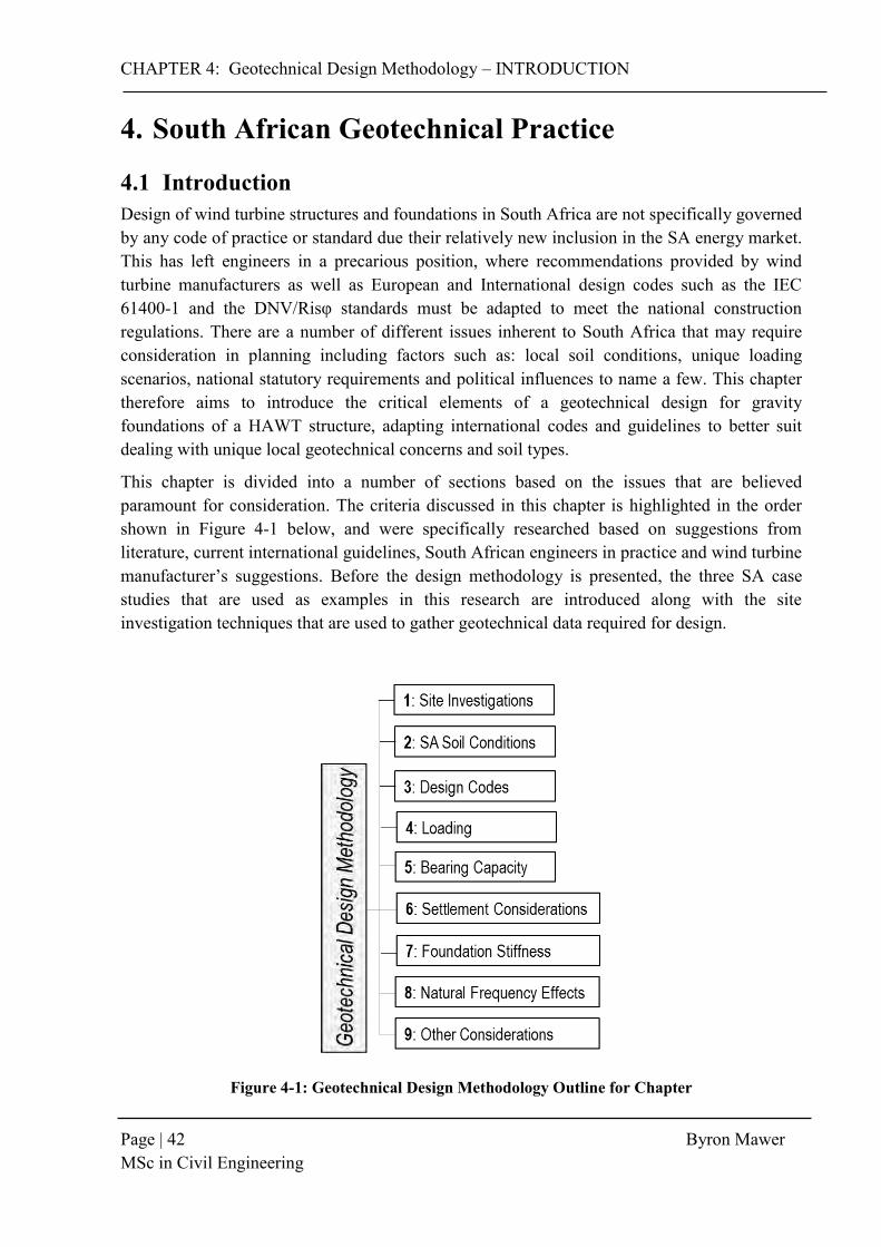
CHAPTER 4: Geotechnical Design Methodology – INTRODUCTION
Page | 42 Byron Mawer MSc in Civil Engineering
4. South African Geotechnical Practice
4.1 Introduction Design of wind turbine structures and foundations in South Africa are not specifically governed by any code of practice or standard due their relatively new inclusion in the SA energy market. This has left engineers in a precarious position, where recommendations provided by wind turbine manufacturers as well as European and International design codes such as the IEC 61400-1 and the DNV/Risφ standards must be adapted to meet the national construction regulations. There are a number of different issues inherent to South Africa that may require consideration in planning including factors such as: local soil conditions, unique loading scenarios, national statutory requirements and political influences to name a few. This chapter therefore aims to introduce the critical elements of a geotechnical design for gravity foundations of a HAWT structure, adapting international codes and guidelines to better suit dealing with unique local geotechnical concerns and soil types.
This chapter is divided into a number of sections based on the issues that are believed paramount for consideration. The criteria discussed in this chapter is highlighted in the order shown in Figure 4-1 below, and were specifically researched based on suggestions from literature, current international guidelines, South African engineers in practice and wind turbine manufacturer’s suggestions. Before the design methodology is presented, the three SA case studies that are used as examples in this research are introduced along with the site investigation techniques that are used to gather geotechnical data required for design.
Figure 4-1: Geotechnical Design Methodology Outline for Chapter

CHAPTER 4: South African Geotechnical Practice – SITE INVESTIGATIONS
Page | 43 Byron Mawer MSc in Civil Engineering
4.2 Site Investigations 4.2.1 Soil Parameters for Design Before any engineering judgement can be made on the type of foundations most suitable for a site, information about the soil that will support the structure must be gathered and analysed. This is the purpose of the geotechnical site investigation. Since any geotechnical design is only as good as the soil data available (Beales, 2012), the site investigation is possibly one of the most important aspects of the planning process for wind turbine foundations, perhaps even for all large scale foundations. As for most structures, the key geotechnical issues and checks that are required for wind turbine footings include:
1) Bearing capacity,
2) Settlement (Total and Differential),
3) Consolidation Settlement (if applicable), and
4) Stability (Overturning & Sliding).
Due to the dynamic nature of turbine loading, two further essential criteria are:
1) Soil stiffness, and
2) Effects of dynamic loading.
Each of these design criteria inherently possess an associated limit for which a wind turbine structure can be safely built and operated without the structure failing or experiencing excessive movement. The allowable limits of these design criteria or, factors of safety, as they are commonly called, can be theoretically calculated using developed geotechnical theory or empirical relationships. All of these equations or empirical relationships require input parameters based on the soil properties of the proposed development site which, when accurate, ensure that each structure that is erected will be supported adequately by the underlying strata.
Around the world, there are a number of different methods and tests that have been developed in order to ascertain the soil property data required for design. These are commonly split into two categories namely; field tests conducted on site using the in-situ arrangement of soils, and laboratory tests conducted on soil samples taken from a site for testing under controlled conditions. Depending where you are in the world, some methods are more commonly used than others and therefore, test data correlations with specific soil types are more readily available in certain regions of the world. This section therefore highlights the specific parameters required for the geotechnical design of wind turbine foundations and additionally describes the tests and methods used in South Africa to obtain these parameters.

CHAPTER 4: South African Geotechnical Practice – SITE INVESTIGATIONS
Page | 44 Byron Mawer MSc in Civil Engineering
4.2.2 Parameters Required The following information or parameters are generally required in order to conduct the design checks when considering wind turbine footings, as discussed in Section 4.2.1 above. These parameters are of importance for a number of different reasons and have been adapted from work presented by Day (2014): 1. Soil/Rock Profile: A soil/rock profile is obtained by logging the material encountered during the drilling of a borehole. The borehole log as it is often referred is crucial for geotechnical designers because it describes the types of soil found on site. When a lack of data is available, a number of assumptions can be made based on the description given by the borehole logger. A number of relationships for soil properties exist based on physical descriptions, and soil behaviour can be estimated based on physical descriptions and the regional geology. 2. Classification & Atterberg Limits: Soil samples are typically categorised according to the USCS classification system in RSA and certain soils can expect various problems based on the classification group they lie in. Classification is based on the grading of soil particle sizes and other empirical relationships and this can help the designer predict certain issues such as drainage problems, low strength, or occurrence of collapsible fabrics and more. Atterberg limit tests conducted on samples in the lab help predict at what levels of moisture, a soil exhibits elastic, semi-plastic or plastic properties. It can also help predict the level of shrinkage that may occur in the soil when dried. Specific Parameters: LL, PL, SL and Grading. 3. Inherent Soil Properties (Density, Specific Gravity, and Moisture Content): Density and specific gravity of a soil are fundamental, as they are direct indicators of the weight of a soil, which affects the bearing capacity and settlement that a soil will experience. The moisture content of soil also affects the weight of the soil; the type of strength properties exhibited as well as the degree a soil can be compacted. Specific Parameters:, ’, NMC, SG, OMC, MDD etc. 4. Strength Properties: Soil strength is modelled on the theoretical resistance to shearing that soil particles inherently possess. This is typically modelled using the Mohr-Coulomb method that bases the strength of the soil on a combination of the cohesion and the internal soil friction particles exhibit when making contact with each other. These are fundamental parameters for calculating bearing capacity, settlement, and the stiffness of a soil. Specific Parameters: c’, φ’, cu, su 5. Stiffness Parameters: Soil stiffness governs a structures response under high moment loads that the risk of soil failure in rocking. It also can in some circumstances effect the occurrence of differential settlement. It also has a major effect on the resonant frequency of a structure and its response to dynamic loading. Specific Parameters: E’, E0, G0, kϴ

CHAPTER 4: South African Geotechnical Practice – SITE INVESTIGATIONS
Page | 45 Byron Mawer MSc in Civil Engineering
4.2.3 Investigation Methods A number of investigation methods have been developed across the world that either give direct values for soil conditions and parameters or can be linked to these factors through theory. In South Africa, a combination of laboratory testing on samples obtained from site as well as field testing on in-situ soils is conducted in order to obtain these values. The typical tests conducted in SA, specifically used in wind turbine site investigations are mentioned below, including the process, the values obtained, the limitations and the alternatives used in other areas of the world where applicable.
4.2.3.1 Standard Penetration Test (SPT) The SPT is one of the most commonly used and accepted test methods worldwide and is the oldest standardized penetration test available. It works by driving a split spoon sampler; 51mm in diameter into the bottom of a borehole by use of a 63.5kg hammer free falling over a distance of 762mm. The number of blows required by the hammer to penetrate the sampler 450mm over three, 150mm intervals is recorded, and after discarding the values of the first 150mm, the other two blow counts are summed and reported as the SPT N value. There are a number of disadvantages to the test compared to new methods such as the CPT and Pressuremeter test, however due to its wide spread use it is generally accepted worldwide. Its main advantage is the number of empirical relationships that have been developed between the SPT N value and soil properties required for calculating bearing capacity, settlement, stiffness and a number of other criteria. The problem with this is that most of the relationships have been developed for a particular soil type and are not necessarily reflective of all sands for example. For this reason, SPT correlations are used cautiously. Figure 4-2 below shows the differences between the SPT and DPSH apparatus that is discussed in the following section.
Figure 4-2: SPT sampler vs. DPSH Cone Setup Sources: Various – Byrne (2008)
2.00 cm
Cone angle 60°

CHAPTER 4: South African Geotechnical Practice – SITE INVESTIGATIONS
Page | 46 Byron Mawer MSc in Civil Engineering
Many experienced local geotechnical engineers base their assumptions, and suggest further testing based on what is discovered from the SPT test. It is generally found that local companies that conduct site investigations will conduct the SPT or CPT test, with very few being familiar with other types of penetration tests or having the capacity or equipment to conduct these tests. For wind turbine projects, SPT values are commonly reported to give the designer an idea of soil properties combined with the description of the soil layers. At times, such as for estimating the modulus of compressibility (Ev), SPT N correlations are often used.
4.2.3.2 Dynamic Probe Super Heavy (DPSH) The DPSH test is widely used in SA along with the SPT mainly because it can be completed quickly and therefore is very economical (Byrne, 2008). The DPSH is primarily a penetration test, similar to the SPT, as it also uses a 63.5kg hammer dropped through a height of 762mm but instead of a split spoon sampler, a 60°, 50mm diameter cone is placed at the bottom of driving rod and it does not require a pre-drilled borehole to conduct the test. Similarly to the SPT, the number of blows required for the cone to move through 300mm is recorded. This gives a continuous record of penetration that provides an empirical indication of soil consistency and strength. The DPSH has a number of correlations associated to the value, and if the shaft friction generated on the sidewall of the driving rod is taken into account, it has been found the DPSH N values are roughly equivalent to those of SPT N values, although this is highly based on local experience according to Byrne (2008). A study was conducted by MacRobert et al. (2011), where SPT and DPSH values were compared for a number of Cape Town soils in order to generate a relationship between the two values. For 5 out of 6 soils, the relationship given in Equation 5 below provided a reasonable correlation between SPT N’ values and DPSH N values, allowing the conversion of data across tests to suit different needs.
𝑆𝑃𝑇 𝑁′ =𝐷𝑃𝑆𝐻𝑁
0.02𝐷𝑃𝑆𝐻𝑁+0.08 (Eqn 5)
where: SPT N’ = the equivalent SPT N value for the same test DPSHN = the recorded DPSH N value for the test Local geotechnical engineers often use the consistency reported from the DPSH test along with the soil description in order to roughly estimate a bearing capacity of the soil, although there is no formal relationship between the two values. This is generally accepted based on the geotechnical engineer’s judgment although, they are liable if the design is based on this assumption and the structure fails. In this study, when DPSH estimated bearing capacities have been reported, they have generally found to be a limiting value to the theoretically calculated bearing capacity (see Eastern Cape Wind Farm example).

CHAPTER 4: South African Geotechnical Practice – SITE INVESTIGATIONS
Page | 47 Byron Mawer MSc in Civil Engineering
4.2.3.3 Laboratory Tests Standard geotechnical tests are conducted on soil samples that are sent to the laboratory from site in order to classify the soil according to USCS or other classification systems depending on the local standards. This aids in obtaining a number of soil parameters such as specific gravity, unit weight, Atterberg Limits, as well as to obtain the max dry density and optimum moisture content. Generally, these tests are conducted to either SANS, BS or the TMH1 standard and are extremely well practiced across South Africa. Test methods commonly conducted include the sieve analysis and hydrometer tests, liquid limit determination via the Casagrande and Cone Penetration methods, and compaction tests via the CBR and Modified Proctor methods. In order to obtain the shear strength parameters of the soil, it is common for a triaxial test to be conducted on soil samples. Triaxial tests apply pressures in x; y and z directions to the sample, matched to the in-situ stress at the zone of interest, and then increase them until failure occurs. The pressures at failure are then linked to the Mohr-Coulomb failure criterion in order to generate c’ and φ’ values for use in design. Different consolidation and drainage conditions can be applied to the test, which makes it imperative that the designer informs the laboratory under what conditions will give the most reflective values for that particular site. In South Africa, many different test standards can be applied too depending on the Clients request. As triaxial tests are usually one of the more expensive commercial tests, SA geotechnical engineers usually conduct tests, at minimum, on samples from the proposed founding depth, which allows parameters for design (SoilLab, 2014). The values quoted in this study, are generally applicable to the proposed founding depth or to other areas of interest if more than one test was allowed for. Alternatively, shear box tests can be used in order to generate the shear strength properties of the soil although; these tests only initiate failure on a single failure plane that may not be the critical one. This may lead to higher shear strength parameters than what is actually inherent of the material.
4.2.3.4 Point Load Tests for UCS For foundations on rocks, as well as for the medium to hard consistency pedogenic soil layers, penetration tests can usually not be conducted without refusal occurring on the material. Due to this, the majority of rock strength properties are based on the Unconfined Compressive Strength (UCS) of the rock obtained from a laboratory test on core samples taken from the site. The Point Load Index (Is) test is commonly conducted on samples of 36.5mm - 50mm (the size of coring drill bits) with a length of 50mm – 75mm (SoilLab, 2014). The value obtained for the Is is generally related to the UCS through the relationship shown in Figure 4-3. Alternatively, triaxial tests can be conducted on rock samples, although they are far more expensive and more time consuming than the Point Load Index test. The UCS value that is obtained in conjunction with the Rock Quality Index (RQD) obtained during the coring, allows for the strength parameters of the rock to be calculated. This covered in more detail at the end of this section.

CHAPTER 4: South African Geotechnical Practice – SITE INVESTIGATIONS
Page | 48 Byron Mawer MSc in Civil Engineering
Figure 4-3: Point Load Index test correlations with UCS value for Rocks Adapted from: (Byrne, 2008 after Bieniawski, 1973)
4.2.3.5 Testing for Stiffness Parameters
Considering dynamic civil structures are not as common as those with static loads are, wind project sites require additional tests to assess the ability of the soil to resist the cyclic loading caused by the rotation of the wind turbine blades. With an understanding of dynamic theory, the structures resistance to these effects is directly related to the structures global stiffness. The stiffness parameters for a soil that govern this response include the Shear Modulus (G), the damping ratio (ξ) and Poisson’s Ratio (v) with the shear modulus being the most important (as discussed in Section 3.5.4). The additional value of the shear modulus is that it can be used to calculate the modulus of elasticity (E) of a soil through the constitutive relationship shown in Equation 6 below, which can be useful in settlement and stiffness calculations.
𝐸 = 2𝐺(1 + 𝑣) (Eqn 6) where: E = Modulus of Elasticity (MPa) G = Shear Modulus (MPa) v = Poisson’s Ratio There are various lab and field testing methods that can be employed to measure the stiffness parameters. The most critical consideration in deciding which of these tests to use, is based on the level of strain that will be applied to the soil and therefore in what stress-strain behaviour range the values obtained are applicable to. Table 4-1 provides an overview of the testing methods available dependent on strain range applicability. Some of the tests covered in Table 4-1 are more relevant than others and significantly more research has been conducted on the

CHAPTER 4: South African Geotechnical Practice – SITE INVESTIGATIONS
Page | 49 Byron Mawer MSc in Civil Engineering
validity of results from these particular tests than others. Laboratory testing for stiffness parameters is not common in South Africa as there is not significant enough demand for these tests for any local geotechnical laboratory to be able to fund one (SoilLab, 2014). In some instances however, there is a need for dynamic laboratory testing in which samples are sent to foreign labs where the resonant column and cyclic triaxial tests are the most frequently used for well understood and behaved soils (Kumar et al. 2013). For soils with specific problems (such as a collapsible fabric), other equipment such as the cyclic torsional shear test can be more applicable. A current trend in dynamic testing is the use of centrifuge tests as well as cyclic simple shear devices, the former, which is extensively used in South Africa for analysing collapse mechanisms of dolomite sinkholes at the University of Pretoria (Gough, 2014). These devices have specific advantages over their more commonly used alternatives, for example, the centrifuge more realistically represents the actual stress path under loading yet it has the disadvantage that it is extremely expensive to run and therefore it is not likely that it will be used for assessing wind turbine stiffness parameters.
Table 4-1: Table summarizing testing methods for determining dynamic soil parameters
Source: Kumar et al. (2013)
Field Tests Laboratory Tests
Low Strain (< 0.001%)
High Strain (> 0.1%)
Low Strain (< 0.001%)
High Strain (> 0.1%)
Seismic reflection and refraction
Standard Penetration Test (SPT)
Resonant Column test
Cyclic Triaxial test
Continuous Surface Wave Tests (CSW)
Cone Penetration Test (CPT)
Ultrasonic pulse test
Cyclic direct shear test
Spectral and Multi-Channel analysis of surface waves (SASW & MASW)
Dilatometer Test (DMT)
Bender Element test
Cyclic torsional shear test
Seismic borehole survey (Cross-hole, Down-Hole and Up-Hole)
Pressuremeter test (PMT)

CHAPTER 4: South African Geotechnical Practice – SITE INVESTIGATIONS
Page | 50 Byron Mawer MSc in Civil Engineering
Field tests are often more varied in their applications although SPT tests are often the most commonly used due to their general acceptance and availability around the world. The problem with this test is that it is destructive in nature meaning that the test effectively strains the soil beyond its failure point. This does not occur with low strain dynamic loading that occurs in wind turbines and therefore a SPT is only valid for high strain tests (i.e. applicable for earthquake design) where a plastic response is expected, but not for any projects were design is being carried where an elastic response is expected (i.e. low strain range). For wind turbine structures, the expected strain range is within a range of 0.001 – 0.1% which according to Kumar et al. (2013), would fall in an intermediate strain range. For this reason, as well as to ensure that the ground profile is not disturbed, geophysical methods are often used in South Africa to obtain the critical stiffness properties for design. With the turn of the 21st century, geophysical methods have become more popular in measuring static and dynamic soil properties (Byrne, 2014) and have grown to include the seismic borehole survey (Cross-hole, Down-Hole and Up-Hole variations), seismic reflection and refraction and the spectral analysis of surface waves (SASW). In South Africa, the Continuous Surface Wave Test (CSW), which is an upgraded version of SASW’s system, is frequently used to obtain the shear modulus of soils. The CSW test primarily operates by measuring the velocity and length of Rayleigh waves generated by a variable frequency vibrator located directly over the area of interest (see Figure 4-4). The advantage of this test is that the frequency of the vibrator can be altered during the test allowing waves to reach different depths of interest. Generally, for wind turbine sites, depending on the type of material, tests are conducted to a depth of 1.5 to 2 times the breadth of the footing, which is typically 20-30m. A number of geophones are then placed at a specific spacing from the vibrator and are used to detect the stress waves reflected by the soil, by measuring the vertical oscillation of the ground at the surface. The shear modulus is then related to the velocity of the waves by the function shown in Equation 7. The reason the CSW test is preferred over other seismic test methods, is due to the fact that it is quick (up to 4 tests can be conducted per day) which, with 40-50 turbine sites, can be a major time and cost benefit to the project. It is additionally, a non-destructive and non-intrusive test that allows designers to get properties from the materials in-situ and not from samples subject to disturbance or effected by human error. Ultimately, the results are possibly the best approximation of a soil’s stiffness properties.
𝐺 = 𝜌𝑣𝑠2 (Eqn 7)
Where G = shear modulus of soil being tested [MPa] ρ = density of soil being tested [kg/m3] 𝑣𝑠 = velocity of waves passing through soil sample [m/s]

CHAPTER 4: South African Geotechnical Practice – SITE INVESTIGATIONS
Page | 51 Byron Mawer MSc in Civil Engineering
Figure 4-4: CSW test apparatus and function diagram Adapted from: Warren-Codrington (2013)
When reliable test data for stiffness parameters is not available for design, practically, engineers often make assumptions of the stiffness of a soil based on the work by Stroud (1989) which relates the compressibility modulus (Ev’) to the SPT N value and the bearing capacity of the soil. Figure 4-5 below shows this relationship for sandy soils, although relationships for cohesive soils, as well as to the CPT cone resistance rather than the SPT are also available.
Figure 4-5: Drained modulus of compressibility (Ev’) for sands Source: Stroud (1989)
Geophones
Variable Frequency Vibrator
Geophones

CHAPTER 4: South African Geotechnical Practice – SITE INVESTIGATIONS
Page | 52 Byron Mawer MSc in Civil Engineering
4.2.3.6 Summary
A number of test methods have been presented with emphasis being placed on how they are used to obtain soil parameters required for the design of gravity foundations. It should be noted that these methods were chosen due to their popularity of use in South Africa and their applicability specifically to South African designers. Table 4-2 below briefly summarizes the method of calculation, tests used and parameters required for each investigated design criteria:
Table 4-2: Frequently used SA soil tests linked to parameters required for design
Adapted from information from Day (2014)
DESIGN CRITERIA
CALCULATION METHOD PROCESS REQUIRED PARAMETERS
REQUIRED SYMBOL
LABORATORY FIELD
Bearing Capacity
Bearing Capacity Equations & empirical rules
Triaxial Test Shear Box Test
DPSH/DCP Test SPT Test
Shear Strength Soil Properties Depth of water table
c', φ', cu γ, γ' zwt
Settlement Conventional Settlement Analysis,
FEM methods Oedometer Test
Triaxial Test DPSH/DCP Test Plate Load Test
Young’s Modulus Poisson’s Ratio
E' v'
Consolidation Empirical Formulations and
Conventional Equations Oedometer Test -
Consolidation Ratio Settlement Coeff
Cc, Cu μ
Stability Conventional checks for
Sliding & Overturning Triaxial Test
Shear Box Test -
Shear Strength Soil Properties Depth of water table
c', φ', cu γ, γ' zwt
Dynamic Stiffness
Rocking Stiffness requirements Bender Elements
(not advised) CSW Tests
Shear Modulus Poissons Ratio Dynamic Modulus
G', G0
v', Edyn
Durability under
Cyclic Fatigue
Foundation and Soil stiffness requirements
Bender Elements (not advised)
CSW Tests Shear Modulus Poissons Ratio Dynamic Modulus
G', G0
v', Edyn
4.2.4 Other Investigations A critical part of a site investigation for wind turbine projects involves the ground on which the turbines are proposed to be built, but there are two additional investigations that need to be conducted. Due to the sheer size of turbine structures, extremely large plant specifically cranes, are required to aid in the installation of the tower segments and the final placement of the nacelle. The largest of these cranes can have 9 axles and weigh up to 200 tons including counterweights (Liebherr, n.d), and with a transport weight of 108 tons this can be an axle load of up to 12 tons/axle. To put this in context, a lightweight car such as the engineer’s personal car or site vehicle could possibly weigh at a maximum 3500 kilograms. This is equivalent to approximately 3.5 tons over 2 axles which is equivalent to 1.75 tons/axle. This is more than 6 times less than that of a crane required for the installation of the turbine units. With sites often located in areas with no paved road access, this makes the design of haul roads and the crane platforms extremely important for the construction of the turbine.

CHAPTER 4: South African Geotechnical Practice – SITE INVESTIGATIONS
Page | 53 Byron Mawer MSc in Civil Engineering
4.2.4.1 Crane Platform A crane platform is the area of ground that will be used to support its weight as well as its stabilizing arms. As part of the site investigation, it is essential to ensure that the in-situ soil will not experience significant settlement or bearing failure when the crane begins to mobilize or when the stabilizing arms are placed. The stabilizing arm of a crane can often impart localised loads of up to 100 tons on the ground and with a very small cross-sectional area, this can result in point load pressures that can be extremely high. It is therefore essential during the planning phase of a wind energy project, to propose where the crane platform will be placed. Trial pits are normally dug in order to characterize the soil or judge the in-situ soil stiffness in these positions using Dynamic Cone Penetrometer (DCP) tests. Local experience and empirical relationships are then used to judge whether the soil has adequate bearing capacity to support the crane. If the soil is found to be too weak, ground improvement techniques can be used to improve the soil strength temporarily. This is often used in practice in Europe by making use of geogrid reinforcement. A practical example was conducted by NAUE at the Salbatica II Wind Farm in Romania where a stress-strain modulus of only 40-50 MPa was found during the site investigation. The result was large settlements of up 30 cm beneath the crane platform. Only with the inclusion of a number of geosynthetic layers underneath the stabilizing arm could a modulus of 170 MPa be achieved limiting the settlement to an acceptable level (Psiorz, 2014).
4.2.4.2 Haul Roads Due to the location of wind projects sites often being well off established roads in order to minimize visual impacts, wind farms often require the construction of haul roads to not only the get the wind turbine sections but the plant and engineers to the project site. While the cranes generally do not need to stop on the haul roads, and only travel over the road once, heavy vehicles carrying the wind turbine units as well as other construction materials, occurs daily. Repetitive traffic of heavy vehicles applies high cyclic loads to the soil, and if the soil has not been properly investigated to ensure it can resist the high loads from the vehicles, haul roads can start to experience rutting (Figure 4-6) as well as the formation of large potholes that makes them impassable. During the wet season, this can be amplified by water especially in soft clayey soils with very low bearing capacities. Similarly to the crane platform, the position of the haul roads must be planned before the site investigation takes place. Trial pits and DCP tests are also used to judge the in-situ soil stiffness and ultimately the bearing capacity of the roads. Typically, if the in-situ soils are of poor quality, either they need to undergo ground improvement or a new good quality base course material must be imported in order to resist the high repetitive loading. As this option is extremely expensive, cheaper and simpler solutions are often required.

CHAPTER 4: South African Geotechnical Practice – SITE INVESTIGATIONS
Page | 54 Byron Mawer MSc in Civil Engineering
Figure 4-6: Example of the formation of rutting on a poorly designed haul road Source: Cuelho & Perkins (2008)
Particularly suited to South Africa is the relatively cheap inclusion of geosynthetic products. Cuelho & Perkins (2008) conducted an extensive study where different geosynthetic grids and textiles were included under a graded haul road experiencing similar loads of what may be experienced by a transport vehicle or crane that would be used for a wind turbine project. Their results showed that certain geogrid products could improve the time taken for formation of rutting from 10 passes to up to 80 passes of a typical 80 kN equivalent axle load. Problematic pavement layer works for haul roads can be improved in a cost effective manner in this way. This gives the reader an idea of the required scope of a geotechnical site investigation for a wind turbine project, although for a designer, understanding a site investigation and its limitations and using the information found within the report, is arguably the most important factor that effects the theoretical predictions covered in later sections. For this reason, Section 4.3 covers the site investigation data obtained for each of the three representative sites that will be designed for. This data will be used through the forthcoming design sections. Before this is introduced, calculating rock properties using theoretical methods will be discussed.
4.2.5 Rock Properties
4.2.5.1 Using Rock Properties Unlike soils, the properties required for calculating the strength and resistance of rock material cannot be completely acquired through only site investigation techniques and require further analysis in order to produce usable data. Rocks do not always respond in a linear fashion although it would be useful for design if in some way rock properties such as the UCS value, RQD values and other observation based properties could be converted into the linear Mohr-

CHAPTER 4: South African Geotechnical Practice – SITE INVESTIGATIONS
Page | 55 Byron Mawer MSc in Civil Engineering
Coulomb shear strength parameters of c’ and φ’ which could then be used in traditional bearing capacity equations and theories. There are a number of theoretical engineering rock mechanics models that are able to give useable properties to rocks based on application as well as a number of other factors. Before a model is chosen however, it is essential to identify and understand the rock failure mechanism that occurs under loading, as this plays a major role in choosing a model that will yield accurate results and that can produce reasonable design predictions.
4.2.5.2 Types of Rock Failure Rocks fail by various mechanisms depending on aspects including intact rock strength, discontinuities in the bedding, jointing, quality of rock formation and the presence of ground water. Generally, rock failures can be divided into groups depending on the jointing of rocks, the absence of jointing (intact) and special cases of failure (see Figure 4-7). For intact rocks, failure normally occurs under very high loads in either local or general shear (similarly to soils) depending on whether the rock displays brittle or ductile behaviour. Alternatively, if there are very high concentrated loads and the rock has an inherently low compressive strength, localized crushing may occur. For jointed rocks, the expected failure mechanism is reliant on the orientation, spacing and the degree of closure that the joint exhibits. Typically, joints in rocks are a line of weakness in the rock body, allowing failure to occur more quickly through propagation along the length of the joint. Vertically orientated, open joints typically fail in local shear, propagating down the open gap and expanding the width as it fails. Closed vertical joints in disparity, present a general shear failure mechanism with a well-defined failure surface, but will propagate along the weakness inherent of the joint in some way. When the spacing of these joints are wider than the breadth of the footing however, failure will occur as in an intact rock. Rock beds with horizontal joints either fail in tension due to flexure, similar to bending in structural beams, or through punching shear depending on the thickness and relative strength of the layer of rock lying above the joint. Diagonal joints are often the worst case as they generally occur at angles very close to that of Terzaghi’s general or local shear failure angle of 45+φ/2° allowing failure to propagate faster. Adding groundwater that lubricates the joint only exaggerates this problem. Fractured rocks are simply a special case of this where a number of discontinuities exist and failure can propagate through any of the joints. This makes failure in fractured rocks very unpredictable and it is therefore difficult to assign a safe bearing strength to them. Finally, two special cases include the cracking of rocks under high concentrated loads and general shear failure in soft rock, a type of failure of which most geotechnical engineers are familiar. During this study, the type of bedding and jointing was generally assumed, as it was not identified during the site investigation. It was therefore assumed that rocks encountered were to be ductile in nature and therefore general shear failure is expected to be prevalent. This allows for a number of geotechnical bearing capacity theories to be investigated in this regard.

CHAPTER 4: South African Geotechnical Practice – SITE INVESTIGATIONS
Page | 56 Byron Mawer MSc in Civil Engineering
Figure 4-7: Failure mechanisms in rock under concentrated load Adapted from: Hoek & Bray (1981)
4.2.5.3 Hoek-Brown Method One of the models generally accepted around the world for converting rock properties into those of the Mohr-Coulomb criteria is the Hoek-Brown method. It was created in 1980 and has been adjusted and updated over time, but was primarily introduced in order to provide input data for the analyses of underground excavations in hard rock. Initially, it was designed for intact rock specimens but then later adapted to allow for strength reductions due to rock bodies exhibiting varying degrees of jointing. The method also took into account the non-linear behaviour of rocks making it advantageous for use. Initially, the Hoek-Brown process was based in adapting the major (σ1) and minor (σ3) stresses to account for rock strength and jointing (see Equation 8), but due to the fact that slope stability and foundation problems are more easily solved using the shear and normal stress, a means of adapting these stresses was required.
Brittle Rock - Local Shear - Brittle Failure
Ductile Rock - General Shear - Well Defined
Failure Surface
Crushing - Low Compressive
Strength - Soft Rock
Open Vertical Joint - Local Shear - Brittle Failure
Closed Vertical Joint - S<B - General Shear - Well Defined
Failure Surface
Closed Vertical Joint - S>B - Well Defined
Failure Surface
Horizontal Joint - Thin Rigid
Layer - Punching
Tensile Failure
Fractured - General Shear - Irregular failure
surface along joint
Diagonal Joint - General Shear - Threat of
failure along joint
Soft Rock - General Shear - Soft Rock treated
similar to strong soil with collapsible fabric
Horizontal Joint - Thick Rigid
Layer - Tensile Failure
due to flexure
Cracking - High concentrated
loads - Crack propagation
along line of weakness

CHAPTER 4: South African Geotechnical Practice – SITE INVESTIGATIONS
Page | 57 Byron Mawer MSc in Civil Engineering
𝜎1
′ = 𝜎3′ + 𝜎𝑐𝑖(𝑚𝑏
𝜎3′
𝜎𝑐𝑖+ 𝑠)0.5 (Eqn 8)
where: σ1 and σ3 are the major and minor effective principal stresses at failure, σci is the uniaxial compressive strength of the rock material, and mb and s are material constants, where s = 1 for intact rock. In order to account for the nature of rock quality and jointing, empirical relationships with the Geological Strength Index (GSI) was adopted in order to relate observations in the field to strength properties. Using the GSI to calculate a number of factors such as mb and s as well as a (shown below), the principal stresses were then adapted into shear and normal stresses using the Equation 9 & 10 by Balmer (1952):
𝜎𝑛′ =
𝜎1′+𝜎3
′
2−
𝜎1′−𝜎3
′
2∙
𝑑𝜎1′ 𝑑𝜎3
′⁄ −1
𝑑𝜎1′ 𝑑𝜎3
′⁄ +1 (Eqn 9)
𝜏 = (𝜎1′ − 𝜎3
′) ∙√𝑑𝜎1
′ 𝑑𝜎3′⁄
𝑑𝜎1′ 𝑑𝜎3
′⁄ +1 (Eqn 10)
where: 𝑑𝜎1
′ 𝑑𝜎3′⁄ = 1 + 𝑎𝑚𝑏(𝑚𝑏𝜎3
′ 𝜎𝑐𝑖 + 𝑠⁄ )𝑎−1
𝑎 =1
2+
1
6(𝑒−𝐺𝑆𝐼 15⁄ − 𝑒−20 3⁄ )
Using the normal and shear stresses calculated through the method above, the results could be fitted to a Mohr-Coulomb relationship in order to ascertain the shear strength parameters mostly commonly used by geotechnical engineers, c’ and φ’. Hoek (1994) argued that fitting a tangent based approximation of the Mohr-Coulomb curve was in fact an upper bound estimate and suggested rather using a least squares method to obtain a more averaged value for c’ and φ’. This led to the occurrence of the a term in Equation 11 &1 2 below which differs slightly from that suggested by Balmer (1952). Ultimately, the results are the equations for c’ and φ’ (Eqn 11 & 12) shown below:
𝑐′ = 𝜎𝑐𝑖[(1+2𝑎)𝑠+(1−𝑎)𝑚𝑏𝜎3𝑛
′](𝑠+𝑚𝑏𝜎3𝑛′)𝑎−1
(1+𝑎)(1+2𝑎)√1+(6𝑎𝑚𝑏)(𝑠+𝑚𝑏𝜎3𝑛′)𝑎−1 (1+𝑎)(2+𝑎)⁄
(Eqn 11)
𝜑′ = sin−1 [6𝑎𝑚𝑏(𝑠+𝑚𝑏𝜎3𝑛
′)𝑎−1
2(1+𝑎)(2+𝑎)+6𝑎𝑚𝑏(𝑠+𝑚𝑏𝜎3𝑛′)𝑎−1] (Eqn 12)
Additionally to this, a value often used in assessing the settlement of rocks under load is the modulus of deformation. By using the rock properties and classifications available as well as a disturbance factor D, the Hoek-Brown method predicts this value using the Equations 13 &14:

CHAPTER 4: South African Geotechnical Practice – SITE INVESTIGATIONS
Page | 58 Byron Mawer MSc in Civil Engineering
𝐸𝑚 = (1 −
𝐷
2) ∙ 10(𝐺𝑆𝐼−10)/40 for σci > 100 MPa (Eqn 13)
𝐸𝑚 = (1 −𝐷
2)√
𝜎𝑐𝑖
100∙ 10(𝐺𝑆𝐼−10)/40 for σci < 100 MPa (Eqn 14)
From the development of the Hoek-Brown method, the computer software RocLab (now known as RocData) produced by Rocscience Inc., a geotechnical software development company, was created as a simple way to conduct these calculations based purely on 4 input parameters. These parameters include: Uniaxial Compressive Strength (σci or UCS) Geological Strength Index (GSI) The material constant (Mi), and The Disturbance Factor (D). In this study, RocLab was used in order to generate values for c’ and φ’ for rocks. UCS values are obtained directly from the site investigation reports and a GSI value was selected based on the descriptions available in the borehole logs as well as from examples provided by Rocscience. For the Mi and D value, RocLab possess extensive libraries that give approximate values for different rocks conditions. For the purposes of this research, the Mi value suggested by the program’s libraries was used. The D value was primarily developed for tunnel and slope excavation and not for foundation design. In this context, a D value of 0.2 would probably be reflective as very little excavation is required for wind turbines founded in rock compared to that of a tunnel. However, to be conservative and to apply to the general outlines suggested by the program, a value of 0.8 is used to be conservative. An example of the Mohr-Coulomb curve generated by RocLab is shown in Figure 4-8 below.
Figure 4-8: Mohr-Coulomb curve generated for rock by RocLab software

CHAPTER 4: South African Geotechnical Practice – SOIL CONDITIONS
Page | 59 Byron Mawer MSc in Civil Engineering
4.3 South African Soil Conditions South Africa has one of the oldest and diverse geological histories in the world that has in part lead to the country’s abundant mineral reserves that boast extensive stockpiles of coal, gold, platinum and diamonds. The breakdown of this vast geological profile over millennia has led to an extremely varied soil profile, which presents geotechnical engineers and engineering geologists with a number of different founding challenges. The country is well known for its problematic soil regions such as the dolomitic regions of the Transvaal, the abundance of soft clay in previous depositional zones such as Richards Bay as well as the wide spread distribution of soils that present expansive and collapsible fabrics. The reclaimed land of Cape Town and its sudden Granite-Malmesbury Shale transition also present many interesting geotechnical design challenges. Many regions of SA are also dominated by rock, especially very close to the surface, such as in regions of the Karoo and the Northern Cape. As the local soil environments are so diverse, sites were chosen with representative soil data that best depict conditions within the major wind energy development corridors. As the majority of wind turbines will be developed in these corridors, the design procedures and results in this chapter will therefore be the most indicative reference, other than actual project plans, for practicing engineers who will be tasked with designing foundations in these areas A site was chosen within each of the three major wind energy corridors including the South West coast corridor, the Eastern Cape corridor and the Klein Karoo corridor. Each of these development zones contain a number of either existing or planned wind energy projects lying with in them. To ensure that soil data is reflective, the data used in this study was assumed based on site investigation reports from either already existing or currently under development wind projects. The soil data used in this report is based on privileged information and therefore cannot be referenced or referred to directly, therefore a brief overview of the applicable properties are outlined in this section. The locations of these projects are shown roughly in Figure 4-9 on the following page and in order to maintain anonymity the three sites are referred to as:
1. EASTERN CAPE WIND FARM
2. WESTERN CAPE WIND FARM
3. KAROO WIND FARM
This nomenclature will be maintained and referred to throughout this study. The following section introduces and discusses these sites in detail and presents the assumed soil profiles and soil data used during the design methodology in Section 5.

CHAPTER 4: South African Geotechnical Practice – SOIL CONDITIONS
Page | 60 Byron Mawer MSc in Civil Engineering
CORRIDOR 3
CORRIDOR 1
CORRIDOR 2
KAROO WIND FARM
EASTERN CAPE WIND FARM
WESTERN CAPE WIND FARM
Figure 4-9: SA Wind Corridor overlain on hybrid topographical map with wind speed Adapted from: Vortex DC (2015)
4.3.1 Eastern Cape Wind Farm
4.3.1.1 Geology of Site The Eastern Cape area close to the city of Port Elizabeth is generally underlain to varying degrees by the Algoa, Uitenhage and Gamtoos Group rocks with each group contributing to the overlying soil deposits found on the site. According to Almond (2010), Algoa group rocks are typically described as aeolian, coastal and shallow marine sediments formed in the Late Caenozoic period. The group can generally consist of six successive formations ranging in age from the Late Miocene through to the Holocene period. In chronological order, these can include the Bathhurst, Alexandria, Nanaga, Salnova, Nahoon and Schlem Hoek formations. Almond (2010) further states that due to the high content of fine shell material, the dominant sediment types often include very lime rich calcareous sandstones (both marine and aeolian), sandy and shelly clastic limestones, conglomerates and coquinite. After many years of deposition, solution and repreciptation of carbonate minerals; tough, white surface pedogenic calcretes form in varying degrees throughout the soil profile, especially with in the Nanaga formations. The presence of pedogenic calcrete is especially problematic to foundation designers as the degree of formation can significantly affect the strength expected from the material. The Gamtoos group rocks generally also include calcareous minerals, feldspathic units as well as phyllite. The rocks of the group also typically weather to form a red silty sand type soil with reasonable strength.

CHAPTER 4: South African Geotechnical Practice – SOIL CONDITIONS
Page | 61 Byron Mawer MSc in Civil Engineering
0.0 m
1.5 m
24.4 m 25.5 m
30.0 m
0.0m – 1.50 m: No material recovered.
1.50 m – 24.42 m: Light brown becoming light reddish brown with depth, silty fine SAND. 24.40 m – 25.50 m: Light greyish brown, slightly silty fine SAND with poorly to moder-ately well-formed CALCRETE. 25.50 m – 30.00 m: Light reddish brown, silty fine SAND with occasional poorly formed CALCRETE.
SOIL DESCRIPTION:
NO WATERTABLE
INTERCEPTED DURING
INVESTIGATION
4.3.1.2 Soil Profile Information pertaining to in-situ soil conditions was available up to a depth of 30m with the soil profile commonly consisting of light brown to red silty fine sand deposits with varying degrees of calcrete formation. Over 10+ profiles, calcrete layers with thicknesses between 0.4 – 3.0m were encountered with generally thicker profiles being found at depth. Calcrete layers were also found at depths ranging from 1.5m to 30m, with an overall trend of increasing degree of formation with depth. One of these profiles was selected for use as the design example indicative of an Eastern Cape Wind Farm. The borehole log, shown in Figure 4-10 below, is typical of the site and includes a thick deposit (roughly 23m) of light brown to red silty fine sand starting from a depth of 1.5m and extending to a depth of 24.4m. This was followed by a 1m light grey silty fine sand including poorly formed calcrete pedogenics. From 25.5m to 30m, the profile exhibited a 4.5m thick reddish silty fine sand deposit including deposits of well-formed calcrete.
Figure 4-10: Eastern Cape Wind Farm assumed soil profile and description Water was not encountered to depth. There were also no indicators in the soil profile of a fluctuating water level. For these reasons, water was assumed to occur well below the foundation base. It is important to note that ground water levels should be checked periodically in order to ensure that this remains the case. The design would require revision if water was encountered within the zone of influence of the foundation base which is commonly between one to two times the breadth of the footing (1B – 2B).

CHAPTER 4: South African Geotechnical Practice – SOIL CONDITIONS
Page | 62 Byron Mawer MSc in Civil Engineering
4.3.1.3 Soil Properties Certain soil properties were obtained by sending a number of samples from each profile for laboratory testing. Tests were conducted in order to classify the soil including a grain size analysis and Atterberg Limit tests. CBR tests were conducted in order to calculate the MDD and OMC values and a single triaxial test was conducted on the soil at the proposed founding depth. Samples were also taken to calculate the natural moisture content at varying depths. Field techniques employed included DCP testing to a depth of 3.5m within a borehole adjacent trial hole as well as DPSH tests to the same depth. During the borehole logging a SPT test was also conducted. Finally, core samples of the well-formed calcrete formations were sent to the laboratory in order to ascertain the UCS of the material. A summary of the soil data assumed for this case study based on this information is shown in Table 4-3 below:
Table 4-3: Summary of assumed soil data for Eastern Cape Wind Farm
Silty Fine Sand Classification
Depth LL PL SL (%) Classification
1.8 m 19 5 1.5 SILTY SAND
7.5 m 21 4 2.5 SILTY FINE SAND
20 m ND SP 0.5 SLIGHTLY SILTY FINE SAND
CBR Test Results
Depth MDD (kg/m3) OMC (%) NMC (%) bulk (kN/m3) v
1.8 m 2003 10.3 11 18.6 0.3
7.5 m 2039 8.9 3.2 19.2 0.3
20 m 2013 9.4 1.7 18.9 0.28
Triaxial Test Results
Depth ϕ (°) c (kPa)
3.5m 31.5 12
Field Test Results
Depth DCP (kPa) DPSH (kPa)
2.5 260 280
3.2 290 320
4.0 320 400+
Calcrete Strength Test Results
Depth (m) Point Load
Index UCS (MPa) RQD (%)
25 0.86 19.9 9

CHAPTER 4: South African Geotechnical Practice – SOIL CONDITIONS
Page | 63 Byron Mawer MSc in Civil Engineering
0.0
1.0
2.0
3.0
4.0
5.0
6.0
7.0
8.0
9.0
10.0
11.0
12.0
13.0
14.0
15.0
0 50 100 150 200 250 300 350 400
Dep
th (
m)
G0 (MPa)
4.3.1.4 CSW Test Results As wind turbines often have an extremely high moment component to their loading, foundation design requirements often dictate a minimum soil stiffness in order to avoid differential settlement of the base in rocking. As this often governs design of turbine foundations, calculating these stiffness values accurately is often of great importance to the designer to optimize their design. As soil stiffness is reliant on the soil mass’ stress-strain relationship, it is important that accurate values for Young’s modulus for the soil can be calculated. In South Africa, these values are derived from the small strain Shear Modulus (G0) most commonly obtained from Continuous Surface Wave (CSW) testing which was discussed in detail in Section 4.2.3. The assumed results for the relevant CSW tests from the Eastern Cape Wind Farm site that have been used in the design are shown in Figure 4-11 below:
Figure 4-11: Assumed CSW test results for Eastern Cape Wind Farm Format adapted from Heymann (2014)

CHAPTER 4: South African Geotechnical Practice – SOIL CONDITIONS
Page | 64 Byron Mawer MSc in Civil Engineering
4.3.1.5 Expectations for design based on soil data This site’s soil profile is made up predominantly of silty fine sands, which from laboratory tests, exhibit soil properties that are indicative of good founding conditions. Based on SPT, DCP and DPSH data, this soil is found to be reasonably dense from depths of 3m and therefore the site can generally be expected to require little to no compaction before work commences. This also means that a 3 meter depth would be a suitable founding depth for the EC design example. The most important consideration for this soil is assessing the effect that the poor to well-formed calcrete beds have on bearing strength. Calcrete is known to be a pedogenic material that is extremely variable in nature, and therefore extreme care is needed when founding on it. With the absence of a water table combined with the aforementioned facts surrounding density and strength of the soil, it is expected that there will be favourable conditions for the use of shallow gravity footings for this design.
4.3.2 Western Cape Wind Farm
4.3.2.1 Geology of Site The geology of the South West coast near the towns of Langebaan and Vredenburg is dominated by the calcareous sands of the Langebaan formation, which overlies a region of the Cape Granite Suite group rocks that forms part of the granite batholith intrusion, which is prominent in the West Coast region. The Langebaan formation rocks, which forms part of the greater Sandveld group, are quaternary aeolian deposits of calcium rich dune sands. After many years of deposition, solution and repreciptation of carbonate minerals; tough, white surface pedogenic calcretes form in varying degrees in the soil profile generally close to the surface. After many years of cyclic water movement through the soil profile, the calcareous layers are generally underlain by various degrees of weathered and residual granite material forming stiff to very stiff clay and silt materials before meeting hard granite bedrock.
4.3.2.2 Soil Profile For the WC site, over 40+ boreholes were conducted with varying conditions being found across the site. Some boreholes indicated a dominant calcrete profile underlain by granite bedrock while others showed a profile dominated more by residual granite material such as stiff clays and sandy silts. As founding on calcrete material will be addressed as part of the design of the Eastern Cape Wind Farm scenario and will be discussed in detail in Section 5.8.1, this scenario will rather focus on the complexities of constructing foundations on stiff clays and silts as characterized in the borehole log shown on the following page. The profile as shown in Figure 4-12, begins with a thin top layer of hillwash material followed by pedogenic silt material. After a 2.0m depth, there are layers of varying thickness of silt and clay materials that have formed because of the decomposition of the underlying granite material. The profile ends with hard granite bedrock.

CHAPTER 4: South African Geotechnical Practice – SOIL CONDITIONS
Page | 65 Byron Mawer MSc in Civil Engineering
0.0 m
1.1 m
9.0 m
10.4 m
19.4 m
2.0 m
27.2 m
30.0 m
0.00 m – 1.10 m: Loose to medium dense sandy SILT. Hillwash. 1.10 m – 2.0m: Stiff, slightly ferruginised fine gravelly sandy SILT. Pedogenic
2.0 m – 9.0m: Very stiff to stiff, clayey fine gravelly sandy SILT. Residual Granite. 9.0 m – 10.4 m: Stiff sandy gravelly clayey SILT. Reworked Residual Granite. 10.4 m – 19.4 m: Firm to stiff, fine gravelly sandy CLAY. Residual Granite. 19.4 m – 27.2m: Very stiff, fine gravelly sandy CLAY. Becoming Very soft rock. Residual Granite. 27.2 m – 30.0m: Medium to Hard Rock. Granite Bedrock.
NO WATER TABLE INTERCEPTED IN BORE-HOLE
SOIL DESCRIPTION:
Figure 4-12: Assumed Western Cape Wind Farm Soil Profile
4.3.2.3 Soil Properties Soil properties were assumed based on lab tests results for samples from the borehole shown in Figure 4-12 above. A number of assumptions were also made from analysing the available borehole logs, as laboratory test reports for this site were privileged, and only a limited amount of geotechnical data could be provided for analysis. The available information included the results of 6 CSW tests, a number of borehole logs, and 2 laboratory test results that included the results of a consolidated undrained triaxial test and point load tests on rock samples. The water table was not encountered on site and was believed to lie far below the zone of influence of the footing. A summary of the assumed data based on these results are available in Table 4-4.
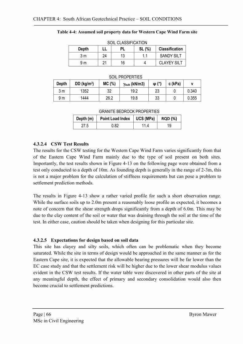
CHAPTER 4: South African Geotechnical Practice – SOIL CONDITIONS
Page | 66 Byron Mawer MSc in Civil Engineering
Table 4-4: Assumed soil property data for Western Cape Wind Farm site
SOIL CLASSIFICATION
Depth LL PL SL (%) Classification
3 m 24 13 1.1 SANDY SILT
9 m 21 16 4 CLAYEY SILT
SOIL PROPERTIES
Depth DD (kg/m3) MC (%) bulk (kN/m3) ϕ (°) c (kPa) v
3 m 1352 32 19.2 23 0 0.340
9 m 1444 26.2 19.8 33 0 0.355
GRANITE BEDROCK PROPERTIES
Depth (m) Point Load Index UCS (MPa) RQD (%)
27.5 0.82 11.4 19
4.3.2.4 CSW Test Results The results for the CSW testing for the Western Cape Wind Farm varies significantly from that of the Eastern Cape Wind Farm mainly due to the type of soil present on both sites. Importantly, the test results shown in Figure 4-13 on the following page were obtained from a test only conducted to a depth of 10m. As founding depth is generally in the range of 2-3m, this is not a major problem for the calculation of stiffness requirements but can pose a problem to settlement prediction methods. The results in Figure 4-13 show a rather varied profile for such a short observation range. While the surface soils up to 2.0m present a reasonably loose profile as expected, it becomes a note of concern that the shear strength drops significantly from a depth of 6.0m. This may be due to the clay content of the soil or water that was draining through the soil at the time of the test. In either case, caution should be taken when designing for this particular site.
4.3.2.5 Expectations for design based on soil data This site has clayey and silty soils, which often can be problematic when they become saturated. While the site in terms of design would be approached in the same manner as for the Eastern Cape site, it is expected that the allowable bearing pressures will be far lower than the EC case study and that the settlement risk will be higher due to the lower shear modulus values evident in the CSW test results. If the water table were discovered in other parts of the site at any meaningful depth, the effect of primary and secondary consolidation would also then become crucial to settlement predictions.

CHAPTER 4: South African Geotechnical Practice – SOIL CONDITIONS
Page | 67 Byron Mawer MSc in Civil Engineering
0.0
1.0
2.0
3.0
4.0
5.0
6.0
7.0
8.0
9.0
10.0
0 50 100 150 200 250 300
Dep
th (
m)
G0 (MPa)
Figure 4-13: Assumed CSW Test Results for Western Cape Wind Farm Adapted from Heymann (2014)
4.3.3 Karoo Wind Farm
4.3.3.1 Geology of Site The geology of Worcester, in the northern part of the Western Cape, is often considered to be in the region of the Klein Karoo, which is dominated by rocks of the Cape Supergroup with occasional intrusions of the Karoo Supergroup dolerites. The site itself has very little to no soil present, with only a 0.2-0.5m covering of top soil evident during the investigation. The underlying rock is distributed varyingly between Table Mountain group sandstones, dolerite formations formed during the volcanic events that led to the formation of the Drakensburg Mountains and finally, some deposited mudstone most likely part of the nearby Cedarburg Formation. Of all the sites, the geological history of this site and its surrounding area is the most critical to the predictions of foundation behaviour, as the rock will form the founding layers for this site. Knowledge of the mechanics behind the formation of fold mountains during the Cape orogeny may also help explain the cause of jointing and discontinuities of rock on this site, which has already been highlighted as a crucial aspect of the for founding on sites dominated by shallow rock.

CHAPTER 4: South African Geotechnical Practice – SOIL CONDITIONS
Page | 68 Byron Mawer MSc in Civil Engineering
0.0 m
1.5 m
4.5 m
9.5 m
30.0 m
0.0m – 1.50 m: Slightly weathered, closely jointed, light grey, medium grained, medium bedded, MEDIUM HARD ROCK SANDSTONE
1.50 m – 4.5 m: Highly weathered, loosely jointed, medium grained, medium bedded, SOFT ROCK SANDSTONE. 4.5 m – 9.5 m: Moderately weathered, grey, medium jointed, medium grained, medium bedded, HARD ROCK SANDSTONE. 9.5 m – 30.00 m: Unweathered, closely jointed, dark grey, medium bedded, VERY
HARD ROCK SANDSTONE.
SOIL DESCRIPTION:
NO WATERTABLE
INTERCEPTED DURING
INVESTIGATION
4.3.3.2 Soil Profile Assumed geotechnical data for Karoo case study was based on over 15+ boreholes that were conducted, with varying conditions being found across the site. This site was generally dominated by rock very close to the surface and extended to depth. The rock found was to be generally medium grained and exhibited various degrees of bedding, weathering, jointing and hardness. As sandstone was by far the dominant of the three rock types found on site, a borehole profile of purely varying degrees of sandstone formation was chosen for the design. The profile (Figure 4-14) begins with a thin top layer of medium hard slightly weathered sandstone followed by a highly weathered layer of softer rock of the same origin. After a depth of 4.5m, the sandstone becomes harder ranging from moderately spaced joints to closely spaced joints to depth. In general, unweathered closely jointed very hard sandstone generally dominates the profile. Additionally, no ground water was encountered on the site.
Figure 4-14: Assumed Karoo Wind Farm Soil Profile
4.3.3.3 Soil Properties Soil properties for this site are obtained slightly differently because it is made up almost completely by rock. Core samples were originally sent for laboratory testing in order to obtain UCS values and CSW tests were conducted to obtain the stiffness parameters however, no shear strength properties were available. In order to make use of the traditional bearing capacity equations, the Hoek-Brown method (as discussed in Section 4.2.5) was used in order to convert the UCS values and the Geological Strength Index (GSI) - based on the jointing and quality of rock formation - into the useable linear Mohr-Coulomb shear strength parameters (c’ and φ’). The results for the profile of this site are shown in Table 4-5:
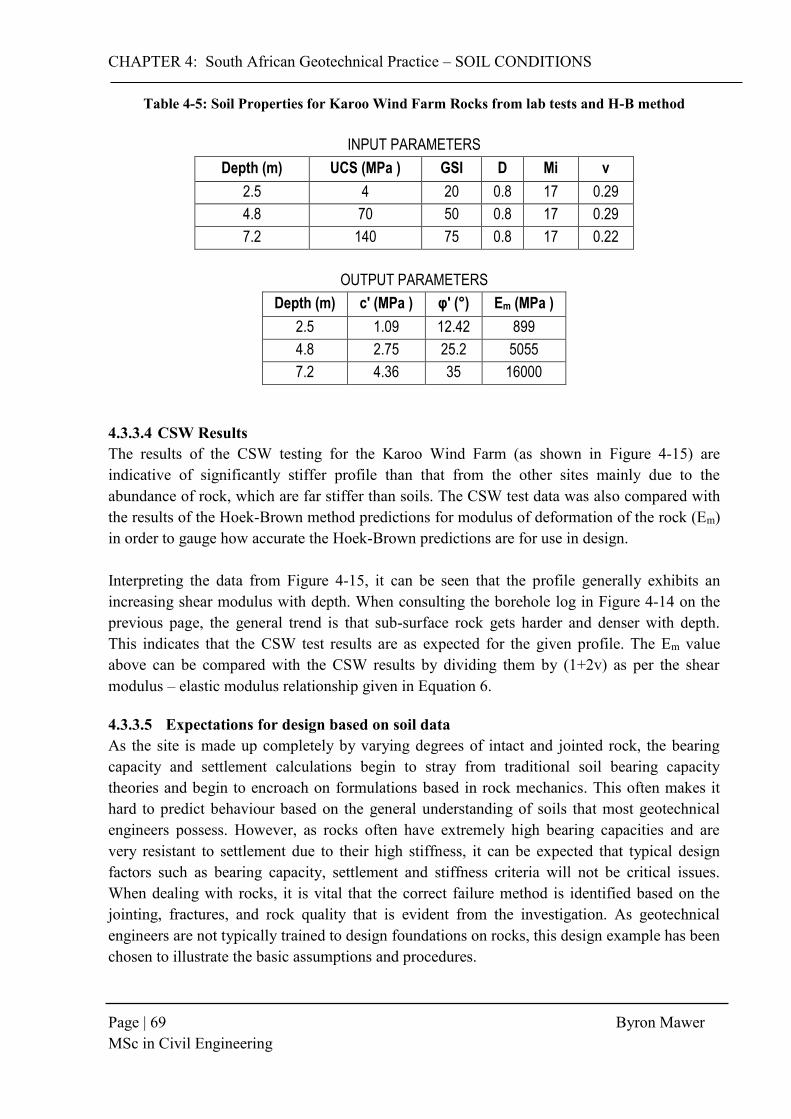
CHAPTER 4: South African Geotechnical Practice – SOIL CONDITIONS
Page | 69 Byron Mawer MSc in Civil Engineering
Table 4-5: Soil Properties for Karoo Wind Farm Rocks from lab tests and H-B method
INPUT PARAMETERS
Depth (m) UCS (MPa ) GSI D Mi v
2.5 4 20 0.8 17 0.29
4.8 70 50 0.8 17 0.29
7.2 140 75 0.8 17 0.22
OUTPUT PARAMETERS
Depth (m) c' (MPa ) φ' (°) Em (MPa )
2.5 1.09 12.42 899
4.8 2.75 25.2 5055
7.2 4.36 35 16000
4.3.3.4 CSW Results The results of the CSW testing for the Karoo Wind Farm (as shown in Figure 4-15) are indicative of significantly stiffer profile than that from the other sites mainly due to the abundance of rock, which are far stiffer than soils. The CSW test data was also compared with the results of the Hoek-Brown method predictions for modulus of deformation of the rock (Em) in order to gauge how accurate the Hoek-Brown predictions are for use in design. Interpreting the data from Figure 4-15, it can be seen that the profile generally exhibits an increasing shear modulus with depth. When consulting the borehole log in Figure 4-14 on the previous page, the general trend is that sub-surface rock gets harder and denser with depth. This indicates that the CSW test results are as expected for the given profile. The Em value above can be compared with the CSW results by dividing them by (1+2v) as per the shear modulus – elastic modulus relationship given in Equation 6.
4.3.3.5 Expectations for design based on soil data As the site is made up completely by varying degrees of intact and jointed rock, the bearing capacity and settlement calculations begin to stray from traditional soil bearing capacity theories and begin to encroach on formulations based in rock mechanics. This often makes it hard to predict behaviour based on the general understanding of soils that most geotechnical engineers possess. However, as rocks often have extremely high bearing capacities and are very resistant to settlement due to their high stiffness, it can be expected that typical design factors such as bearing capacity, settlement and stiffness criteria will not be critical issues. When dealing with rocks, it is vital that the correct failure method is identified based on the jointing, fractures, and rock quality that is evident from the investigation. As geotechnical engineers are not typically trained to design foundations on rocks, this design example has been chosen to illustrate the basic assumptions and procedures.

CHAPTER 4: South African Geotechnical Practice – SOIL CONDITIONS
Page | 70 Byron Mawer MSc in Civil Engineering
0.0
2.0
4.0
6.0
8.0
10.0
12.0
14.0
16.0
18.0
20.0
0 1000 2000 3000 4000 5000 6000 7000
Dep
th (
m)
G0 (MPa)
Figure 4-15: Assumed CSW Test Results for Karoo Wind Farm Adapted from: Heymann (2014)
CHAPTER 5: Geotechnical Design Methodology – DESIGN CODES
Page | 71 Byron Mawer MSc in Civil Engineering
5. Geotechnical Design Methodology
5.1 Design Codes & References Possibly one of the most challenging parts of designing wind turbine foundations specifically for South African conditions is the fact that there is very little mention of wind turbine structures in the national construction code, the SANS. This makes it extremely challenging for an engineer to ensure that the foundation design for a wind turbine is not only structurally safe but also meets all required limitations of the South African standard. This is exemplified by the fact that even if the standards are met, the structure will almost certainly not be safe due to the code’s limited acknowledgement of these types of systems. This in contrast to typical steel and concrete infrastructure which are essentially safe when designed to the national standards.
This has resulted in local designers making use of international design codes as well as those that have been generated by research institutions in order to ensure that the foundations are planned to be as safe as possible. As there are a number of documents available that all deal with the design of wind turbine footings, this section serves to highlight the important documents consulted for checking each of the vital criteria of HAWT gravity foundation design. As discussed in the previous section, the geotechnical planning checks for turbine foundation include bearing capacity, settlement, consolidation and stability while the dynamic loading criteria include soil stiffness and the effect of dynamic loads on natural frequency.
5.1.1 DNV/Risφ (2002) In 2002, the Det Nortske Veritas and the Risφ National Laboratory in Denmark collaborated in order to publish a document entitled, “Guidelines for the Design of Wind Turbines”. This is possibly the most citied text concerning the design of wind turbine foundations and offers thorough background to wind loading as well as to bearing capacity and stiffness considerations. The DNV/Risφ research discusses all aspects of wind turbine design including the planning of each component of a turbine structure from the basic workings of the system to the complex finite element models that are used to assess the suitability of the tower and foundation design. While the majority of theory and key citations are indicated in this text, the approach is extremely broad and no detailed calculations are available which at times make it extremely difficult to apply to a practical example. The hope is that this study addresses this problem. SECTIONS APPLICABLE TO: Loading Bearing Capacity Settlement Considerations Foundation Stiffness
CHAPTER 5: Geotechnical Design Methodology – DESIGN CODES
Page | 72 Byron Mawer MSc in Civil Engineering
5.1.2 Manufacturers Technical Guidelines Each wind turbine manufacturer produces and provides their clients engineer with their own technical specifications and foundation design guidelines that are unique to each turbine class that they produce. These technical guidelines provide the engineer with all unfactored loading as well as the load cases that are considered critical for the design of the foundation for their specific turbine model. Without this data, the engineer would be required to model the wind turbine system and expected airflow according the load cases described in IEC 61400-1. As this is a complex process, the foundation engineer is not required to fulfil this task, and the manufacturer is fully liable for this information. They additionally provide all limits on soil stiffness requirements as well as fatigue load information for the structural design. In South Africa, the majority of existing wind farms have been contracted to Vestas, General Electric, Siemens or Nordex as the turbine manufacturer, therefore for the purpose of this research, technical specifications and foundation design guidelines for Vestas and General Electric 2-3 MW turbines were used. Besides the loading data, the technical guidelines also provide guidance on the approach and applicability of certain methods as well as key considerations for the design of the foundation. This is often directly linked to discussions in the DNV/Risφ (2002) and the manufacturers often refer to this guideline. Without these two documents, wind turbine foundation design becomes significantly more reliant on the engineer to model the foundation-tower-turbine system in some sort of discrete or finite element modelling software that can handle the analysis of airflow as a turbulent fluid. This could potentially increase the design period significantly for engineers inexperienced with modelling dynamic fluid flow. The only major limitation to these guidelines are that they require a certain amount of clarification by the manufacturer and can be very difficult to comprehend without either a thorough knowledge of the field or aid from the manuals author. This being stated, these guidelines will be used thoroughly and referred to throughout the design process. SECTIONS APPLICABLE TO: Loading Bearing Capacity Settlement Considerations Foundation Stiffness Natural Frequency Effects Other Considerations

CHAPTER 5: Geotechnical Design Methodology – DESIGN CODES
Page | 73 Byron Mawer MSc in Civil Engineering
5.1.3 IEC 61400-1 The IEC 61400-1 is the International Electro-technical Commission code that specifically deals with the operation and installation of wind turbines. While the code mainly deals with design standards for the mechanical and electrical components of a wind turbine, it forms the basis of the load cases that need to be considered by the foundation designer. It also includes a relatively small section on structural design (for the tower) as well as guidelines for the planning and construction of a wind turbine. This is the international standard for which any client must abide by when erecting a wind turbine and therefore is an important document. This being stated, it provides very little practical value for the planning of foundations other than the load cases already discussed. As the manufacturers provide the loading and the applicable load cases, having taken into account these standards, it generally is not critical for the foundation designer to consult the code. For the Contractor however, it would be strongly advised that the code be reviewed before construction begins. SECTIONS APPLICABLE TO: Site Investigations (possibly) Loading
5.1.4 Svensson (2008) Svensson’s (2008) master’s thesis entitled “Design of Foundations for Wind Turbines” is a practical design guide for the structural design of wind turbine foundations in Sweden. While this is not strictly a design code, it provides valuable insight into the technical application of test data and the DNV/Risφ guidelines and how it is practically applied when planning a wind turbine foundation. While focused on structural design, geotechnical aspects are dealt with briefly in order to acquire dimensions of the foundation for structural purposes. It serves as a good reference for any designer who fails to understand the practical design calculations required and the permutations of these calculations that are unique to wind turbine foundations, however there are no explanations available and the engineer is left to assess exactly how Svensson conducted the design. The geotechnical portion of the study is also limited to bearing capacity calculations by the DNV/Risφ method and it is not compared or ratified in any way. It possibly could serve as a good study for engineers who are required to structurally design the foundation according to the Eurocode, but not for geotechnical considerations. SECTIONS APPLICABLE TO: Loading Bearing Capacity Structural Design

CHAPTER 5: Geotechnical Design Methodology – DESIGN CODES
Page | 74 Byron Mawer MSc in Civil Engineering
5.1.5 Warren-Codrington (2013) Research conducted by Warren-Codrington was the first notable South African research published by the University of Cape Town concerning geotechnical wind turbine foundation design for South African soils. Amongst other things, this research investigated specifically construction over pedocrete soils. This is particularly relevant considering a large amount of current and proposed wind turbine sites are founded upon pedocrete soils in South Africa. The research presents good background as to the mechanics and operations of wind turbines and how this effects foundation design, as well as the current theory that is applicable to each of the criteria addressed in this research. It also provides a very a good background as to the effect of the dynamic action of the turbine and how it effects the structure, the soil and the interface between the two bodies. It’s one disadvantage is that it provides no practical examples and does not apply the knowledge that is presented. For any designer who is planning to design a foundation on pedocrete soils, this text would provide valuable insight and should be consulted. Additionally, reference should be made by any designer who does not understand structural dynamics of turbines or the theory behind this research. SECTIONS APPLICABLE TO: Site Investigations (possibly) Bearing Capacity Foundation Stiffness Natural Frequency Effects Other Considerations
5.1.6 Das (2011) Bearing capacity calculations for soils that are not uniform in nature often rely on traditional theory that has been adapted in some way. For layered soils, soils close to bedrock, and for founding on rock, Das provides a number of revised bearing capacity models for assessing the effect of the turbines loading. While any geotechnical theory book could be used, Principles of Foundation Engineering by Das is considered one of the best texts on geotechnical foundation theory in the world. For this study therefore, Das has been referred to on a number of occasions. SECTIONS APPLICABLE TO: Bearing Capacity Settlement

CHAPTER 5: Geotechnical Design Methodology – LOADING
Page | 75 Byron Mawer MSc in Civil Engineering
5.2 Loading As the starting point in most structural or geotechnical analyses, the loading on a wind turbine structure is of vital importance to the foundation, which must channel these loads to the ground. The loading on a HAWT is a complex combination of many attributing loads, all of which contribute differently to the overall design requirements of the foundation. In this case, load is defined as the actions and forces that cause the resultant stresses, strains and deformations within the wind turbine structure, from the tip of the blade to the tower base, including all active machinery in the system. These loads are in turn, transferred through the structure to the foundation and ultimately to the supporting soil. This section aimed to define the type of loads that a wind turbine experiences as well as how these loads are accounted for the design phase. Finally, a summary of the loads used in this research is presented.
5.2.1 Types of Loads The types of loads experienced by a wind infrastructure is governed by three main factors including 1) the external conditions the structure is subjected too, 2) the type of turbine and its placement with respect to other turbines and, 3) the dynamic effects and subsequent response to time dependent loading. A wind turbine structure is subjected to the following forces according to IEC 61400-1:
1) Gravitational and Inertial Loads: These are static and dynamic forces that are caused by gravity, such as the weight of the structure or, the vibrations and rotations inherent in a turbine due to the rotor. Seismic activity may also fall in this category although it was not considered in this work. These types of forces primarily make up the vertical dead loads acting on the structure and are often governed by the type of turbine and its placement on site.
2) Aerodynamic Loads: These are defined by the fact that they are caused directly from the moving airflow and its interaction with the structure, most notably the blades of the turbine. The intensity and type of load is governed by a number of factors including average wind speed, turbulence of the airflow, rotational design speed of the rotor, air density, the shape of rotor blade and any interactive effects between blade and the airflow such as drag. As this is one of the most critical loads for wind turbines, the airflow and dynamics have been discussed in detail in Section 3.5.1.
3) Actuation Loads: Actuation loads are placed on the structure due to the operation and control of the wind turbine internal mechanisms by the operator. This includes the effect of controlling the speed of rotation of the rotor and the pitch and elevation of each individual blade. This is usually considered an abnormal load and is not usually accounted for in normal operation state conditions. The effects are often negligible in the ultimate limit state design where the worst case loading assumes the structure is parked. They can become important when considering long term fatigue of the structural components of the foundation depending on the control mechanism selected.

CHAPTER 5: Geotechnical Design Methodology – LOADING
Page | 76 Byron Mawer MSc in Civil Engineering
4) Other Loads (e.g. ice loads, wake loads, impact loads etc.): Other loads can include any force or pressure experienced by the structure that is not included above that may have a significant effect on the system response. The most common is that for ice loads in Europe but this is not applicable in South Africa. The idea of a wake load can also be important depending on the planned layout of the turbines.
Ultimately, these loads can be reduced down to 4 simple forces and moments based on direction and magnitude of action. Each resultant load or moment is generally provided by the manufacturer after they have conducted considered numerous airflow models and practical tests for their specific turbine within its operating limits. These loads are described below using the Vestas load schedule (2013) symbols and shown in Figure 5-1:
1) Fres: A lateral load acting through the hub of the turbine due to aerodynamic forces,
2) Fz: A vertical downward acting load typically consisting of the weight of the structural elements,
3) Mres: A moment caused at the base due to Fres acting at hub height,
4) Mz: Additional moments caused due to rotation of the turbine, subsidiary aerodynamic effects and other loading.
Figure 5-1: Simplified loading on Wind Turbine Structure for design
x z
y
Fz
Fres
Mz
Mres

CHAPTER 5: Geotechnical Design Methodology – LOADING
Page | 77 Byron Mawer MSc in Civil Engineering
While it is important to understand where the load originates from, as well as the specific force and moments considered in design, there are also a number of factors specific to wind turbines that need to be understood before the loading provided by the manufacturers will be applicable and representative of that which will occur on any given site.
5.2.2 Factors affecting Loading
5.2.2.1 Turbine Spacing The majority of the load classes above are dependent on reasonably fixed or site dependent factors such as those associated with a certain model of turbine or the expected environmental conditions in an area. The aerodynamic forces however, can be significantly affected by the placement of each individual turbine on the development site. As Lynn (2012) explains, the main task of a wind turbine is to extract as much of the kinetic energy from the moving airstream as possible. As turbines make contact with the airstream they cause a wake, similar to that of water behind a motorboat. This wake is essentially an area of turbulent air, which can adversely affect any turbines that come after it. This leads to the important idea of spacing of wind turbines on the development site. On an ideal flat site with a constant wind direction in one direction, the downwind spacing (as shown in Figure 5-2) is recommended to be at about 8-10 times the rotor diameter to limit wake losses to less than 10%. Crosswind spacing is more complicated as wind often does not occur in a uniform direction on any given site, leading to the turbine adjusting to the dominant wind direction by use of their yaw motors. This can lead to scenarios when, if the turbine has moved through a 90° change in yaw direction, the original downwind spacing has become the crosswind spacing and vice-versa. In practice, to balance this problem as well as to keep the project economical, a minimum crosswind spacing of 5 times the rotor size is suggested. Each site however, must be assessed and judged according to its unique topography and the model of turbine that is being installed. As long as a potential site for a wind farm has been planned correctly, taking into account these factors as well as those discussed in Section 3.4.4, the loading data provided from suppliers will give representative data for the structural and geotechnical design of foundations (Bonnett, 2005).
Figure 5-2: Spacing of wind turbines on site to increase aerodynamic efficiency
Adapted from: Lynn (2012)
Prevailing
wind
crosswind
spacing
downwind
spacing
turbine
CHAPTER 5: Geotechnical Design Methodology – LOADING
Page | 78 Byron Mawer MSc in Civil Engineering
5.2.3 Load Cases & Design Situations Structural and geotechnical designs often make use of Ultimate Limit State (ULS) and Serviceability Limit State (SLS) methods, which consider the most critical loading cases that a structure will experience in its lifetime. With the design satisfying the most serious limit state to an acceptable safety factor, the structure will be capable of withstanding any loading scenario that it may experience in its service life. However, due to the dynamic nature of a wind turbine’s loading as well as the number of operational states that a turbine can be placed in (see Section 3.4.4), a number of scenarios need to be checked to ensure that at no point will the structural system fail.
The IEC61400-1 provides a table listing the number of different loading scenarios that must be checked in order satisfy that the system has been adequately modelled for the worst-case conditions that a turbine may experience. The table (as shown in Table 5-1) indicates the type of check that must be performed (ULS, SLS of FLS) with a U, S or an F as well as a suggestion of whether normal, abnormal or construction related load factors should be applied during calculation (signified by N, A or T). This is listed for each mode of operation of a turbine while experiencing either normal wind conditions (NWM) which indicates the use of a Normal Wind Speed Model or extreme wind conditions (EWM) which indicates that the Extreme Wind Speed Model is being used for force calculations. Subsequent tables and clauses provide each load factor that should be included in the design.
These load calculations can often be extremely complicated requiring advanced modelling software in order to generate reliable data. As stated before, for engineers tasked with the structural and geotechnical design of foundations, the combined critical load combinations of all loading is made available by the wind turbine manufacturer for use. All liability for this information is taken by the manufacturers and meets all requirements of IEC 61 400-1. Some of the loading information, such as that from GE, provides the Design Load Case (DLC) that the provided loads are in line with. To fully understand these concepts, consider a General Electric 1.6-82.5, 79.7m HH 1.6 MW wind turbine. Provided by the supplier is a document entitled, “Load Specification for the Foundation of the Wind Turbine Generator System”. This document provides all the essential data described above including loads factored for normal operation as well as loads for cold climates where snow and frost are likely. As can be seen in Table 5-2, a number of critical DLC’s have been provided for as these have been found to be critical for the design of the foundation by the supplier. All other load cases that do not appear in the table, have been checked in regard to the stability of the mechanical design criteria of the tower which does not fall under the scope of the foundation engineer’s requirements (GE, 2013b), or those load cases did not produce the worst case scenarios relevant to the foundation engineers job. Additionally, Table 5-3 provides the loading data from the Vestas V112 3MW 1540rpm HH 94 IEC2A turbine.

CHAPTER 5: Geotechnical Design Methodology – LOADING
Page | 79 Byron Mawer MSc in Civil Engineering
Table 5-1: Table 2 extracted from IEC61400-1 for load cases and combinations Source: (IEC 61400-1, 2005)
DESIGN SITUATION DLC WIND CONDITION TYPE OF
ANALYSIS
PARTIAL SAFTEY
FACTORS
1) Power Production 1.1 NWM U N
1.2 NWM F -
1.3 ETM U N
1.4 ECD U N
1.5 EWS U N
2) Power Production + Fault State 2.1 NWM U N
2.2 NWM U A
2.3 EOG U A
2.4 NWM F -
3) Start-Up 3.1 NWP F
3.2 EOG U N
3.3 EDC U N
4) Shut Down 4.1 NWP F -
4.2 EOG U N
5) Emergency Shut Down 5.1 NWM U N
6) Parked 6.1 EWM (50 Year) U N
6.2 EWM (50 Year) U A
6.3 EWM (1 Year) U N
6.4 NWM F -
7) Parked with fault 7.1 EWM (1 year) U A
8) Transport, Assembly, Maintenance, Repair 8.1 NWM U T
8.2 EWM (1 year) U A
The loads stated in Table 5-3 are each used as per the criterion that is being checked. Only one load is missing from the tables on the following page, which is the weight of the gravity foundation itself. This is assumed based on approximate dimensioning made at the beginning of the design process. These assumptions are constantly required to be re-evaluated as each of the design values is checked.

CHAPTER 5: Geotechnical Design Methodology – LOADING
Page | 80 Byron Mawer MSc in Civil Engineering
Table 5-2: Loads acting at tower base for GE 1.6MW turbine Source: (General Electric, 2013b)
Table 5-3: Loads acting at tower base for Vestas 3MW turbine Source: (Vestas, 2013)
EXTREME LOADS Normal Operation
DLC Mres Mz Fres Mz PLF
[kNm] [kNm] [kN] [kN] [-] [-]
3.2 66700 -353 695 -4590 1.35
Abnormal Load Case
DLC Mres Mz Fres Mz PLF
[kNm] [kNm] [kN] [kN] [-] [-]
6.2 85100 1551 1031 -4500 1.35
NORMAL LOADS Normal Operation
DLC Mres Mz Fres Mz PLF
[kNm] [kNm] [kN] [kN] [-] [-]
1.1 49100 731 554 -4620 1.35
DLC Fx Fy Fz Mx My Mz Fr Mr γ Vhub Vdir
[kN] [kN] [kN] [kNm] [kNm] [kNm] [kN] [kNm] [m/s] [deg]
EXTREME LOAD CONDITIONS
2.1 2783.3 -1.7 -13.2 2354.8 -4583.1 781.5 13.3 4649.2 1.35 25 -8
6.2 2164.3 -544.1 -14.8 -802.5 -2218.4 34314.2 544.3 34385.8 1.1 48.5 95.3
1.5 2681.3 37.3 566.1 310.2 37885.6 -920.8 567.4 37896.8 1.35 32.5 -8
2.2 2134.1 84.8 -253.7 4368.4 -21306 -6335.6 267.5 22228.4 1.1 11.7 -8
1.5 2644.1 68.8 -496 1092 -41160 -3030.5 500.8 41271.8 1.35 12.1 -8
6.2 2080.7 -517.1 51.4 -1244.2 -1954 35425.9 519.6 35479.8 1.1 41.3 31.8
1.5 2681.3 37.3 566.1 310.2 37885.6 -920.8 567.4 37896.8 1.35 32.5 -8
1.5 2644.1 68.8 -496 1092 -41160 -3030.5 500.8 41271.8 1.35 12.1 -8
FOUNDATION LIFT-OFF CONDITIONS
1 1992.1 -9.3 222 -28 16080.2 1678.5 222.2 16167.6 1
OVERTURNING LOAD CONDITIONS
2.2 1996.1 7.5 456.1 -548.8 35013 983.6 456.2 35026.8 1
SLIDING LOAD CONDITIONS
2.2 1940.1 77.1 -230.7 3971.3 -19369 -5759.7 243.2 20207.6 1
6.2 1967.6 -494.7 -13.4 -729.5 -2016.7 31194.7 494.8 31260.3 1
SHEAR FAILURE LOAD CONDITIONS
1.5 2644.1 68.8 -496 1092 -41160 -3030.5 500.8 41271.8 1.35
TENSION LOADING IN PILES CONDITION
1.1 2002.5 -17.5 305.5 -3.2 20678.2 2396.1 306.1 20816.5 1

CHAPTER 5: Geotechnical Design Methodology – LOADING
Page | 81 Byron Mawer MSc in Civil Engineering
5.2.4 Dimensioning & Gravity Load To calculate the weight of the gravity footing, it is required to make a number of dimensioning and shape assumptions regarding the foundation. In this research, it was decided that two typical foundation shapes would be investigated, specifically a square and circular footing. This was limited to the bearing capacity calculations, with the round footing being carried through the rest of the design due to it being the most common foundation geometry employed in South Africa. The initial dimensions for the footing were based on the preliminary design of a Nordex N90/2500 2.5 MW turbine (see Appendix A) from which, the following dimensions were assumed for the footing sizes (Table 5-4 & Figure 5-3). In this case, any turbine dimensions may be assumed as it only serves as a starting point in design. The Nordex N90 system in this case, was simply adapted due to the simplicity of the design document as compared with other manufacturer’s.
Table 5-4: Assumed dimensions for square and circular footings
tfooting (m)
Bfooting (m)
Lfooting (m)
Dfooting (m)
dfooting (m)
SQUARE 2.0 18.0 18.0 - -
CIRCULAR 2.0 - - 18.0 2.7
Assumptions
Df 3.0 m
γreforced concrete 24.0 kN/m3
Dsteel stub 4.0 m
tfooting
Bfooting
Lfooting
1b)
Dfooting
tfooting
Dsteel stub
dfooting
1a)
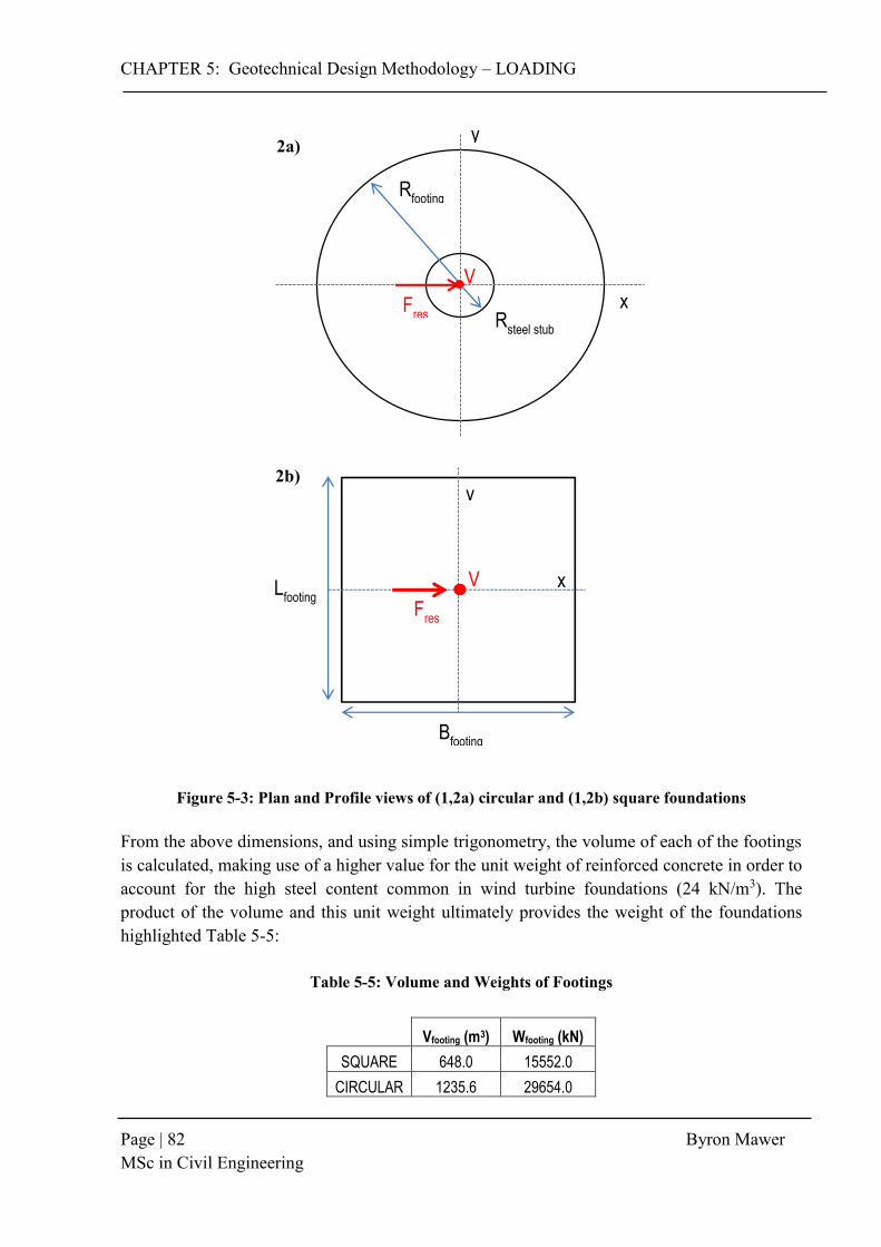
CHAPTER 5: Geotechnical Design Methodology – LOADING
Page | 82 Byron Mawer MSc in Civil Engineering
Lfooting
F
res
V
Bfooting
y
x
Figure 5-3: Plan and Profile views of (1,2a) circular and (1,2b) square foundations
From the above dimensions, and using simple trigonometry, the volume of each of the footings is calculated, making use of a higher value for the unit weight of reinforced concrete in order to account for the high steel content common in wind turbine foundations (24 kN/m3). The product of the volume and this unit weight ultimately provides the weight of the foundations highlighted Table 5-5:
Table 5-5: Volume and Weights of Footings
Vfooting (m3) Wfooting (kN)
SQUARE 648.0 15552.0
CIRCULAR 1235.6 29654.0
x
y
Rfooting
Fres
V
Rsteel stub
2a)
2b)
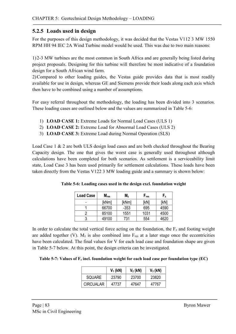
CHAPTER 5: Geotechnical Design Methodology – LOADING
Page | 83 Byron Mawer MSc in Civil Engineering
5.2.5 Loads used in design For the purposes of this design methodology, it was decided that the Vestas V112 3 MW 1550 RPM HH 94 IEC 2A Wind Turbine model would be used. This was due to two main reasons: 1) 2-3 MW turbines are the most common in South Africa and are generally being listed during project proposals. Designing for this turbine will therefore be most indicative of a foundation design for a South African wind farm. 2) Compared to other loading guides, the Vestas guide provides data that is most readily available for use in design, whereas GE and Siemens provide their loads along each axis which then have to be combined using a number of assumptions. For easy referral throughout the methodology, the loading has been divided into 3 scenarios. These loading cases are outlined below and the values are summarized in Table 5-6:
1) LOAD CASE 1: Extreme Loads for Normal Load Cases (ULS 1) 2) LOAD CASE 2: Extreme Load for Abnormal Load Cases (ULS 2) 3) LOAD CASE 3: Extreme Load during Normal Operation (SLS)
Load Case 1 & 2 are both ULS design load cases and are both checked throughout the Bearing Capacity design. The one that gives the worst case is generally used throughout although calculations have been completed for both scenarios. As settlement is a serviceability limit state, Load Case 3 has been used primarily for settlement calculations. These loads have been taken directly from the Vestas V122 3 MW loading guide and a summary is shown below:
Table 5-6: Loading cases used in the design excl. foundation weight
Load Case Mres Mz Fres Fz
- [kNm] [kNm] [kN] [kN]
1 66700 -353 695 4590
2 85100 1551 1031 4500
3 49100 731 554 4620 In order to calculate the total vertical force acting on the foundation, the Fz and footing weight are added together (V). Mz is also combined into Fres at a later stage once the eccentricities have been calculated. The final values for V for each load case and foundation shape are given in Table 5-7 below. At this point, the design criteria can be investigated.
Table 5-7: Values of Fz incl. foundation weight for each load case per foundation type (EC)
V1 (kN) V2 (kN) V3 (kN)
SQUARE 23790 23700 23820
CIRCUALAR 47737 47647 47767

CHAPTER 5: Geotechnical Design Methodology – BEARING CAPACITY
Page | 84 Byron Mawer MSc in Civil Engineering
5.3 Bearing Capacity 5.3.1 Introduction The bearing capacity is defined as the ability of a soil to support the loads that are applied to it. A number of different bearing capacity theories have been established over the last century to theoretically calculate bearing failure in soils. These have all been based on Terzaghi’s 1940 theory, which predicts that shear failure between soil particles beneath a foundation is the main cause. This has been developed into a number of modified concepts including Meyerhof’s, Hansen’s and Vesic’s theories. For wind turbine foundations, bearing capacity calculations are made more complicated by the large moments that are applied to the structure. This has been dealt with by a number of theories including Meyerhof’s Effective Area method as well as by Highter & Anders (1985), which both reduce the effective area of the foundation base to generate new effective dimensions of the footing that account for the effect of the moment that is applied. Additionally, the pressure distribution from the applied loading is affected by the application of the moment, making it more biased in the direction that the moment is placed. In this section therefore, the bearing capacity calculations for gravity foundations is outlined taking into account the complex structural loading that is applied to it. A number of theories will be used and compared based on the soil conditions for each of the 3 representative sites. This is discussed and compared before concluding the chapter. Full design calculation sheets are also available for each site in Appendix B. The explanation of the design calculations follows the Eastern Cape example, although up to Section 5.3.5, where the bearing capacity equations are presented, the process followed is the same for all design examples as these calculations are not dependent on site-specific characteristics.
5.3.2 Effective Area & Eccentricity In order to calculate the effect that a moment applied to a foundation has on the bearing capacity of the footing, an effective area is calculated to obtain new effective dimensions. When Meyerhof first introduced his modified bearing capacity equation, he suggested the “effective area method” for calculating bearing capacities of foundations subject to eccentric loads. If the eccentricity is not given, it can be calculated by Equation 15:
𝑒 =𝑀𝑟𝑒𝑠
𝑉 (Eqn 15)
This was then used in order to calculate the new effective dimensions using the equations for rectangular footings (Eqn 16):
𝐵′ = 𝐵 − 2𝑒 (Eqn 16) 𝐿′ = 𝐿 − 2𝑒 with 𝐴𝑒𝑓𝑓 = B′ ∙ L′

CHAPTER 5: Geotechnical Design Methodology – BEARING CAPACITY
Page | 85 Byron Mawer MSc in Civil Engineering
This method has been modified numerous times by various authors depending on the application of loads that is being planned. DNV/Risφ (2002) developed a method specific to circular and rectangular foundations for wind turbines that gives the most suitable parameters for design. Based on the loads and moments from Table 5-6 & 5-7, the eccentricity values were calculated, and are summarized in Table 5-8 below:
Table 5-8: Eccentricity values for square and circular footings for each load case
e1 (m) e2 (m) e3 (m)
SQUARE 2.59 3.32 1.90
CIRCUALR 1.40 1.79 1.03
The method for calculating the effective area clearly differs by foundation shape and therefore methods for both circular and rectangular foundations are shown below.
5.3.2.1 Circular Foundation The effective area that leads to the most critical result for the bearing capacity of the foundation is the generally the effective area that should be chosen. For a circular foundation, this is generally represented best by an ellipse centred laterally at a spacing of e from the foundation centre. The effective area is then calculated using Equation 17:
𝐴𝑒𝑓𝑓 = 2[𝑅2 arccos (𝑒
𝑅) − 𝑒√𝑅2 − 𝑒2] (Eqn 17)
With effective dimensions of: (as shown in Figure 5-4):
𝑏𝑒 = 2(𝑅 − 𝑒)
𝑙𝑒 = 2𝑅√1 − (1 −𝑏
2𝑅)2
As an ellipse is a shape that is usually hard to work with practically for the design, a rectangle with the same effective area as the ellipse is assumed (see Figure 5-4), centred over the same centre as the ellipse (at a lateral spacing of e from the foundation centre). These shapes and dimensions are then used in design. Table 5-9 presents the values calculated for the load cases discussed in Section 5.3.2
𝑏𝑒𝑓𝑓 =𝑙𝑒𝑓𝑓
𝑙𝑒𝑏𝑒
𝑙𝑒𝑓𝑓 = √𝐴𝑒𝑓𝑓𝑙𝑒
𝑏𝑒
For an octagon shaped base, the same formulas apply simply using the radius of the inscribed circle of the base (radius from centre of base to centre of one of the flat edges of the shape).

CHAPTER 5: Geotechnical Design Methodology – BEARING CAPACITY
Page | 86 Byron Mawer MSc in Civil Engineering
e
x
R
y
L.C le
be
beff
leff
Aeff
Table 5-9: Effective area and dimensions for circular foundations
Load Case Aeff (m2) be (m) le (m) leff (m) beff (m)
1 287.85 18.21 20.81 18.14 15.87
2 271.71 17.43 20.69 17.96 15.13
3 303.26 18.94 20.90 18.29 16.58
Figure 5-4: Calculation of effective area of circular shaped gravity footing Source: Adapted from (DNV/Risφ, 2002)
5.3.2.2 Rectangular Foundation Similarly to a circular footing, the effective area that leads to the most critical result for the bearing capacity of the foundation is the generally the effective area that should be chosen. For a rectangular or square foundation however, two eccentricity checks are calculated and the one that generates the smallest effective area is used. Unlike a circle, a square or rectangle has two distinct axes of symmetry. For calculation of Aeff, the first scenario accounts for an eccentricity occurring over only one of the axes of symmetry, while Scenario 2 accounts for the eccentricity occurring over both. Both calculations make use of Equation 18 and are highlighted in Figure 5-15 & 5-16 below.. FOR SQUARE FOOTING:
𝐴𝑒𝑓𝑓 = 𝑏𝑒𝑓𝑓 ∙ 𝑙𝑒𝑓𝑓 (Eqn 18)
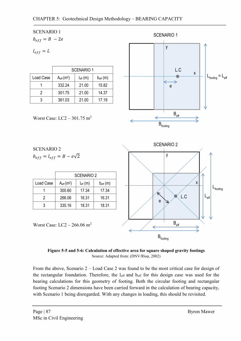
CHAPTER 5: Geotechnical Design Methodology – BEARING CAPACITY
Page | 87 Byron Mawer MSc in Civil Engineering
Bfooting
Lfooting
= Leff
y
x
e
L.C
Beff
SCENARIO 1 SCENARIO 1 𝑏𝑒𝑓𝑓 = 𝐵 − 2𝑒
𝑙𝑒𝑓𝑓 = 𝐿
SCENARIO 1
Load Case Aeff (m2) leff (m) beff (m)
1 332.24 21.00 15.82
2 301.75 21.00 14.37
3 361.03 21.00 17.19
Worst Case: LC2 – 301.75 m2
SCENARIO 2 𝑏𝑒𝑓𝑓 = 𝑙𝑒𝑓𝑓 = 𝐵 − 𝑒√2
SCENARIO 2
Load Case Aeff (m2) leff (m) beff (m)
1 300.60 17.34 17.34
2 266.06 16.31 16.31
3 335.16 18.31 18.31
Worst Case: LC2 – 266.06 m2
Figure 5-5 and 5-6: Calculation of effective area for square shaped gravity footings Source: Adapted from: (DNV/Risφ, 2002)
From the above, Scenario 2 – Load Case 2 was found to be the most critical case for design of the rectangular foundation. Therefore, the leff and beff for this design case was used for the bearing calculations for this geometry of footing. Both the circular footing and rectangular footing Scenario 2 dimensions have been carried forward in the calculation of bearing capacity, with Scenario 1 being disregarded. With any changes in loading, this should be revisited.
Bfooting
y
x
e L.C
Beff
Lfooting
Leff
SCENARIO 2
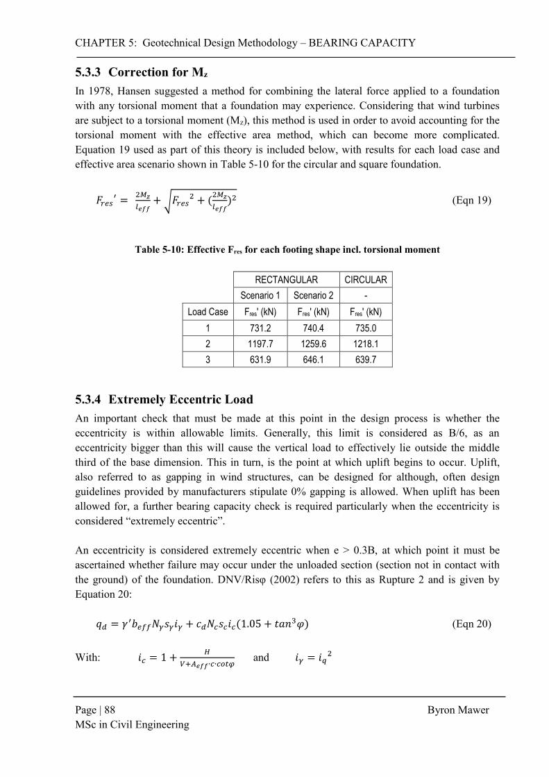
CHAPTER 5: Geotechnical Design Methodology – BEARING CAPACITY
Page | 88 Byron Mawer MSc in Civil Engineering
5.3.3 Correction for Mz In 1978, Hansen suggested a method for combining the lateral force applied to a foundation with any torsional moment that a foundation may experience. Considering that wind turbines are subject to a torsional moment (Mz), this method is used in order to avoid accounting for the torsional moment with the effective area method, which can become more complicated. Equation 19 used as part of this theory is included below, with results for each load case and effective area scenario shown in Table 5-10 for the circular and square foundation.
𝐹𝑟𝑒𝑠′ =
2𝑀𝑧
𝑙𝑒𝑓𝑓+ √𝐹𝑟𝑒𝑠
2 + (2𝑀𝑧
𝑙𝑒𝑓𝑓)2 (Eqn 19)
Table 5-10: Effective Fres for each footing shape incl. torsional moment
RECTANGULAR CIRCULAR
Scenario 1 Scenario 2 -
Load Case Fres' (kN) Fres' (kN) Fres' (kN)
1 731.2 740.4 735.0
2 1197.7 1259.6 1218.1
3 631.9 646.1 639.7
5.3.4 Extremely Eccentric Load An important check that must be made at this point in the design process is whether the eccentricity is within allowable limits. Generally, this limit is considered as B/6, as an eccentricity bigger than this will cause the vertical load to effectively lie outside the middle third of the base dimension. This in turn, is the point at which uplift begins to occur. Uplift, also referred to as gapping in wind structures, can be designed for although, often design guidelines provided by manufacturers stipulate 0% gapping is allowed. When uplift has been allowed for, a further bearing capacity check is required particularly when the eccentricity is considered “extremely eccentric”. An eccentricity is considered extremely eccentric when e > 0.3B, at which point it must be ascertained whether failure may occur under the unloaded section (section not in contact with the ground) of the foundation. DNV/Risφ (2002) refers to this as Rupture 2 and is given by Equation 20:
𝑞𝑑 = 𝛾′𝑏𝑒𝑓𝑓𝑁𝛾𝑠𝛾𝑖𝛾 + 𝑐𝑑𝑁𝑐𝑠𝑐𝑖𝑐(1.05 + 𝑡𝑎𝑛3𝜑) (Eqn 20) With: 𝑖𝑐 = 1 +
𝐻
𝑉+𝐴𝑒𝑓𝑓∙𝑐∙𝑐𝑜𝑡𝜑 and 𝑖𝛾 = 𝑖𝑞
2
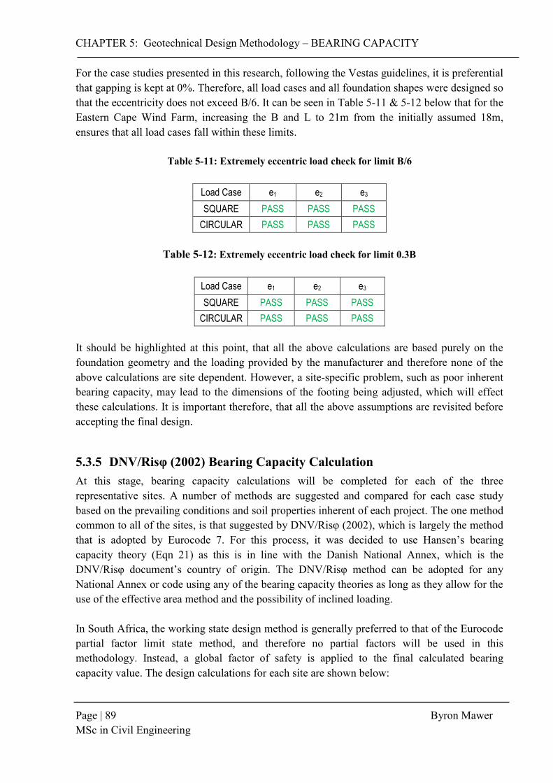
CHAPTER 5: Geotechnical Design Methodology – BEARING CAPACITY
Page | 89 Byron Mawer MSc in Civil Engineering
For the case studies presented in this research, following the Vestas guidelines, it is preferential that gapping is kept at 0%. Therefore, all load cases and all foundation shapes were designed so that the eccentricity does not exceed B/6. It can be seen in Table 5-11 & 5-12 below that for the Eastern Cape Wind Farm, increasing the B and L to 21m from the initially assumed 18m, ensures that all load cases fall within these limits.
Table 5-11: Extremely eccentric load check for limit B/6
Load Case e1 e2 e3
SQUARE PASS PASS PASS
CIRCULAR PASS PASS PASS
Table 5-12: Extremely eccentric load check for limit 0.3B
Load Case e1 e2 e3
SQUARE PASS PASS PASS
CIRCULAR PASS PASS PASS
It should be highlighted at this point, that all the above calculations are based purely on the foundation geometry and the loading provided by the manufacturer and therefore none of the above calculations are site dependent. However, a site-specific problem, such as poor inherent bearing capacity, may lead to the dimensions of the footing being adjusted, which will effect these calculations. It is important therefore, that all the above assumptions are revisited before accepting the final design.
5.3.5 DNV/Risφ (2002) Bearing Capacity Calculation At this stage, bearing capacity calculations will be completed for each of the three representative sites. A number of methods are suggested and compared for each case study based on the prevailing conditions and soil properties inherent of each project. The one method common to all of the sites, is that suggested by DNV/Risφ (2002), which is largely the method that is adopted by Eurocode 7. For this process, it was decided to use Hansen’s bearing capacity theory (Eqn 21) as this is in line with the Danish National Annex, which is the DNV/Risφ document’s country of origin. The DNV/Risφ method can be adopted for any National Annex or code using any of the bearing capacity theories as long as they allow for the use of the effective area method and the possibility of inclined loading. In South Africa, the working state design method is generally preferred to that of the Eurocode partial factor limit state method, and therefore no partial factors will be used in this methodology. Instead, a global factor of safety is applied to the final calculated bearing capacity value. The design calculations for each site are shown below:

CHAPTER 5: Geotechnical Design Methodology – BEARING CAPACITY
Page | 90 Byron Mawer MSc in Civil Engineering
USING HANSEN’S METHOD:
𝑞𝑢𝑙𝑡 = 𝑐𝑁𝑐𝑠𝑐𝑑𝑐𝑖𝑐𝑔𝑐𝑏𝑐 + 𝑞𝑁𝑞𝑠𝑞𝑑𝑞𝑖𝑞𝑔𝑞𝑏𝑞 +1
2𝛾𝐵′𝑁𝛾𝑠𝛾𝑑𝛾𝑖𝛾𝑔𝛾𝑏𝛾 (Eqn 21)
Bearing Capacity Factors: Depth Factors: 𝑁𝑐 = (𝑁𝑞 − 1)𝑐𝑜𝑡𝜑 𝑑𝑐 = 1.0 + 0.4𝑘 or/. 𝑑𝑐 = 0.4𝑘 for φ = 0 𝑁𝑞 = 𝑒𝜋𝑡𝑎𝑛𝜑𝑡𝑎𝑛2(45 +
𝜑
2) 𝑑𝑞 = 1.0 + 2𝑡𝑎𝑛∅(1 − 𝑠𝑖𝑛∅)2𝑘
𝑁𝛾 = 1.5(𝑁𝑞 − 1)tan 𝜑 𝑑𝛾 = 1.0
Shape Factors: where:
𝑠𝑐 = 1.0 + 𝑁𝑞
𝑁𝑐∙
𝐵′
𝐿′ or/. 𝑠𝑐 = 0.2
𝐵′
𝐿′ for φ = 0° 𝑘 =
𝐷
𝐵 for D/B <1 or
𝑠𝛾 = 1.0 − 0.4 𝐵′
𝐿′𝑠𝑖𝑛∅ > 0.6 𝑘 = 𝑡𝑎𝑛−1(
𝐷
𝐵) for D/B >1
𝑠𝑞 = 1.0 + 𝐵′
𝐿′𝑠𝑖𝑛∅
Inclination Factors:
𝑖𝑐′ = 0.5 − √1 − 𝐻𝑖
𝐴𝑓𝐶𝑎 for φ = 0°
𝑖𝑐 = 𝑖𝑞 − 1−𝑖𝑞
𝑁𝑞−1
𝑖𝑞 = [1 − 0.5𝐻𝑖
𝑉+ 𝐴𝑓𝑐𝑎𝑐𝑜𝑡∅]
𝛼1 Use α1 = 3
𝑖𝛾 = [1 − 0.7𝐻𝑖
𝑉+ 𝐴𝑓𝑐𝑎𝑐𝑜𝑡∅]
𝛼2 Use α2 = 3
The following factors for Hansen’s method were obtained from Bowles (1997), although DNV/Risφ (2002) provides slightly adjusted equations for calculating the shape and inclination factors. Both sets of equations were applied, with the most critical values being chosen for use in design. It should also be noted that the g and b factors are assumed to be 1.0 as the ground is assumed not to be sloped or the base to be tilted. Additionally, B’ refers to beff in the rectangular scenarios and be in the circular cases. DNV/Risφ (2002) Factors 𝑠𝛾 = 1.0 − 0.4
𝐵′
𝐿′ 𝑖𝛾 = 𝑖𝑞
2
𝑠𝑞 = 𝑠𝑐 = 1.0 + 0.2 𝐵′
𝐿′ 𝑖𝑞 = 𝑖𝑐 = (1 −
𝐻
𝑉+ 𝐴𝑒𝑓𝑓. 𝑐𝑎. 𝑐𝑜𝑡∅)
2
𝑠𝑐0 = 𝑠𝑐 𝑖𝑐
0 = 0.5 + 0.5 ∙ (1 −𝐻
𝐴𝑒𝑓𝑓. 𝑐𝑎. )
0.5
𝑁𝑐0 = 𝜋 + 2

CHAPTER 5: Geotechnical Design Methodology – BEARING CAPACITY
Page | 91 Byron Mawer MSc in Civil Engineering
For the Eastern Cape Wind Farm, the soil properties obtained from the site investigation (highlighted in Table 5-13) as well as the loading for each of the load cases are used in order to calculate the bearing capacity of the soil. The properties, factors and final bearing capacity calculated using Equation 21 are shown Table 5-13 and 5-14 for a rectangular footing. A global factor of safety of 3 was applied to all qult values in order to obtain the theoretical allowable bearing capacity. This value is then compared to the qapplied calculated in Equation 22 below. Both these values are then compared to the estimated bearing strength obtained through the empirical correlation of the DPSH test. If the qapplied, is less than either the theoretical or the DPSH prediction, the soil is considered to have insufficient bearing capacity and either ground improvement techniques need to be employed or the foundation size must be increased. While this can be a solution, the bigger the foundation gets, the more it weighs, which can ultimately offset any improvement gained by increasing the foundation breadth. This must be judged for every specific design.
Table 5-13: Factors for Hansen bearing capacity calculations for rectangular footing
Soil Parameters Value
Bearing Factors
φ (°) 31.5
Nq 21.86
c (kPa) 12
Nc 34.04
γbulk (kN/m3) 18.90
Nγ 19.18
DPSH: < 320 kPa
Depth Factors
DCP: < 100 kPa
dq 1.04
dc 1.06
dγ 1
Rectangular Footing [after Bowles (1997)]
After DNV/Risφ (2002)
sq sc sγ
sq sc sγ
LC 1 1.522 1.642 0.600
LC 1 1.2 1.2 0.60
LC 2 1.522 1.642 0.600
LC 2 1.2 1.2 0.60
LC 3 1.522 1.642 0.600
LC 3 1.2 1.2 0.60
Rectangular Footing [after Bowles (1997)]
After DNV/Risφ (2002)
iq ic iγ
iq ic iγ
LC 1 0.963 0.961 0.948
LC 1 0.950 0.950 0.903
LC 2 0.937 0.934 0.912
LC 2 0.916 0.916 0.839
LC 3 0.968 0.967 0.955
LC 3 0.957 0.957 0.917

CHAPTER 5: Geotechnical Design Methodology – BEARING CAPACITY
Page | 92 Byron Mawer MSc in Civil Engineering
Table 5-14: Results from Hansen bearing capacity calculations for rectangular footing
RECTANGULAR (Bowles) c q γ qult (kPa) qall (kPa) qreal (kPa)
LC 1 681.5 1889.4 1787.2 4358.1 1450 162.47 PASS
LC 2 662.2 1838.6 1618.0 4118.9 1370 214.88 PASS
LC 3 685.4 1899.9 1901.9 4487.2 1500 124.81 PASS
RECTANGULAR (DNV/Risφ)
LC 1 492.5 1470.0 1702.4 3664.8 1220 162.47 PASS
LC 2 474.6 1416.6 1487.4 3378.6 1130 214.88 PASS
LC 3 496.2 1481.0 1824.6 3801.7 1270 124.81 PASS
In order to calculate the qreal values, the design vertical load needed to be divided by the effective area of the foundation for each applicable load case. However, due to the eccentricity of the load caused by the resultant moment, the distribution of stress is not uniformly distributed through the base. In order to account for this, the following equation, derived from first principles, is used:
𝑞𝑚𝑎𝑥 =𝑄
𝐴𝑒𝑓𝑓(1 +
6𝑒
𝐵𝑒𝑓𝑓) (Eqn 22)
𝑞𝑚𝑖𝑛 =𝑄
𝐴𝑒𝑓𝑓(1 −
6𝑒
𝐵𝑒𝑓𝑓) (Eqn 23)
For example, consider Load Case 2. The total vertical load for the Eastern Cape Wind Farm (V2) was given as 23 700 kN (Table 5-7). This is then divided by Aeff, which equals 266.06 m2 under Scenario 2. This is then multiplied by the factor shown in Equation 22 above. With e equal to 3.31m, and Beff = 16.61m, this produces a qreal value of 214.88 kPa. When calculating qmin using this method, you may obtain a negative answer if Beff is larger than 6e. Typically, using this method, as long as B/6 > e, this qmin value (Eqn 23) can be ignored and the 0% gapping assumption under serviceability limits are still maintained for design. For this site, the empirical bearing capacity based on the DPSH test was given as 320 kPa. As all qreal values were below the qall and the DPSH prediction for all load cases, the rectangular footing of size 21m x 21m was found to be sufficient under the bearing capacity design check. The same method is followed above for a circular footing, obviously with the only adjustments coming in calculating the shape factors. Due to the much higher weight of the circular footing, the qreal values are significantly higher than that of the square footings. For this reason, in order to support the load, the foundation is required to have a diameter of 21m to avoid gapping.

CHAPTER 5: Geotechnical Design Methodology – BEARING CAPACITY
Page | 93 Byron Mawer MSc in Civil Engineering
Table 5-15: Factors for Hansen bearing capacity calculations for circular footing
Soil Parameters
Bearing Factors
φ (°) 31.5
Nq 21.86
c (kPa) 12
Nc 34.04
γbulk (kN/m3) 18.90
Nγ 19.18
DPSH: < 320 kPa
Depth Factors
DCP: < 100 kPa
dq 1.04
dc 1.06
dγ 1
Circular Footing [after Bowles (1997)]
After DNV/Risφ (2004)
sq sc sγ
sq sc sγ
LC 1 1.457 1.562 0.650
LC 1 1.175 1.175 0.650
LC 2 1.440 1.541 0.663
LC 2 1.168 1.168 0.663
LC 3 1.474 1.582 0.637
LC 3 1.181 1.181 0.637
Circular Footing [after Bowles (1997)]
After DNV/Risφ (2004)
iq ic iγ
iq ic iγ
LC 1 0.979 0.978 0.970
LC 1 0.971 0.971 0.944
LC 2 0.964 0.963 0.951
LC 2 0.953 0.953 0.908
LC 3 0.981 0.981 0.974
LC 3 0.975 0.975 0.951
Table 5-16: Results from Hansen bearing capacity calculations for a circular footing
CIRCULAR (Bowles)
c q γ q ult (kPa) q all (kPa) qreal (kPa)
LC 1 659.3 1837.9 1813.5 4310.7 1440 253.46 PASS
LC 2 640.6 1790.3 1727.8 4158.8 1390 300.15 PASS
LC 3 669.9 1864.2 1865.4 4399.5 1470 215.97 PASS
CIRCULAR (DNV/Risφ)
LC 1 492.9 1471.3 1764.1 3728.3 1240 253.46 PASS
LC 2 480.7 1434.8 1649.7 3565.2 1190 300.15 PASS
LC 3 497.5 1485.0 1821.4 3803.9 1270 215.97 PASS
With a DPSH value of 320 kPa for this site, this design is very close to the allowable bearing capacity limit although it is still within the design requirements. As the calculation method is

CHAPTER 5: Geotechnical Design Methodology – BEARING CAPACITY
Page | 94 Byron Mawer MSc in Civil Engineering
exactly the same for each wind farm site using the DNV/Risφ (2002) method, the process for each site will not be highlighted again. Instead, the values obtained from the calculations are presented (Table 5-15 & 5-16) and are explained in light of the site-specific problems that were encountered pertaining to bearing capacity.
5.3.5.1 Western Cape Wind Farm As a whole, the Western Cape Wind Farm typically exhibited soil conditions that were weaker than that of the Eastern Cape Wind Farm. For this reason, it would be expected that the foundation size would need to be enlarged in order to maintain a safe bearing capacity. For this reason, increased dimensions of 21m square and 23m in diameter were required for the square and circular footing respectively. The change in dimensions will affect the loads and eccentricities that are encountered; hence, the loads, eccentricities and new effective area parameters are highlighted in Table 5-17 below:
Table 5-17: Summary of loads, eccentricities and effective areas of footings for WC Wind Farm
V1 (kN) V2 (kN) V3 (kN)
e1 (m) e2 (m) e3 (m)
SQUARE 25758 25668 25788
SQUARE 2.59 3.32 1.90
CIRCULAR 49158 49068 49188
CIRCULAR 1.36 1.73 1.00
CIRCULAR FOOTING
Load Case Aeff (m2) be (m) le (m) leff (m) beff (m)
1 353.21 20.29 22.84 19.94 17.71
2 336.00 19.53 22.74 19.78 16.99
3 369.62 21.00 22.91 20.08 18.41
RECTANGULAR FOOTING
SCENARIO 1 SCENARIO 2
Load Case Aeff (m2) leff (m) beff (m) Aeff (m2) leff (m) beff (m)
1 332.24 21.00 15.82 300.60 17.34 17.34
2 301.75 21.00 14.37 266.06 16.31 16.31
3 361.03 21.00 17.19 335.16 18.31 18.31
RECTANGULAR CIRCULAR
Scenario 1 Scenario 2 -
Load Case Fres' (kN) Fres' (kN) Fres' (kN)
1 729.4 736.9 731.3
2 1189.2 1238.6 1199.7
3 628.0 639.6 631.6
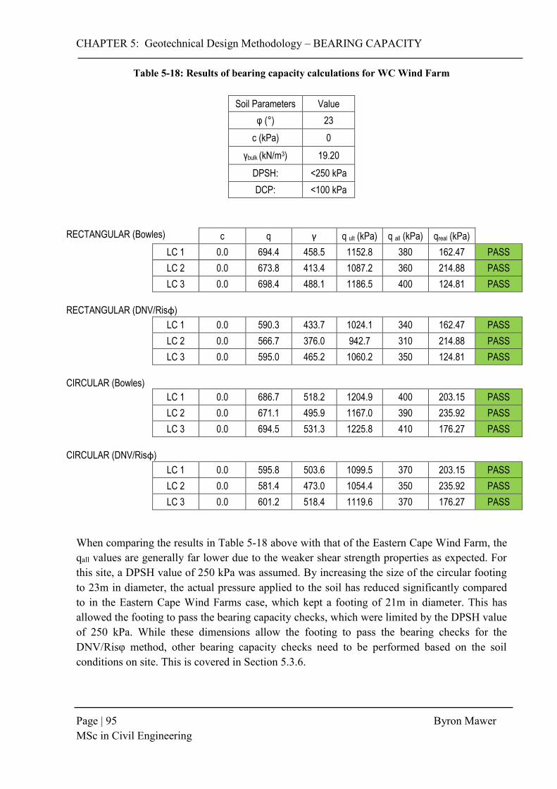
CHAPTER 5: Geotechnical Design Methodology – BEARING CAPACITY
Page | 95 Byron Mawer MSc in Civil Engineering
Table 5-18: Results of bearing capacity calculations for WC Wind Farm
Soil Parameters Value
φ (°) 23
c (kPa) 0
γbulk (kN/m3) 19.20
DPSH: <250 kPa
DCP: <100 kPa
RECTANGULAR (Bowles) c q γ q ult (kPa) q all (kPa) qreal (kPa)
LC 1 0.0 694.4 458.5 1152.8 380 162.47 PASS
LC 2 0.0 673.8 413.4 1087.2 360 214.88 PASS
LC 3 0.0 698.4 488.1 1186.5 400 124.81 PASS
RECTANGULAR (DNV/Risφ)
LC 1 0.0 590.3 433.7 1024.1 340 162.47 PASS
LC 2 0.0 566.7 376.0 942.7 310 214.88 PASS
LC 3 0.0 595.0 465.2 1060.2 350 124.81 PASS
CIRCULAR (Bowles)
LC 1 0.0 686.7 518.2 1204.9 400 203.15 PASS
LC 2 0.0 671.1 495.9 1167.0 390 235.92 PASS
LC 3 0.0 694.5 531.3 1225.8 410 176.27 PASS
CIRCULAR (DNV/Risφ)
LC 1 0.0 595.8 503.6 1099.5 370 203.15 PASS
LC 2 0.0 581.4 473.0 1054.4 350 235.92 PASS
LC 3 0.0 601.2 518.4 1119.6 370 176.27 PASS
When comparing the results in Table 5-18 above with that of the Eastern Cape Wind Farm, the qall values are generally far lower due to the weaker shear strength properties as expected. For this site, a DPSH value of 250 kPa was assumed. By increasing the size of the circular footing to 23m in diameter, the actual pressure applied to the soil has reduced significantly compared to in the Eastern Cape Wind Farms case, which kept a footing of 21m in diameter. This has allowed the footing to pass the bearing capacity checks, which were limited by the DPSH value of 250 kPa. While these dimensions allow the footing to pass the bearing checks for the DNV/Risφ method, other bearing capacity checks need to be performed based on the soil conditions on site. This is covered in Section 5.3.6.

CHAPTER 5: Geotechnical Design Methodology – BEARING CAPACITY
Page | 96 Byron Mawer MSc in Civil Engineering
5.3.5.2 Karoo Wind Farm The Karoo Wind Farm is mostly founded upon rock, which is not particularly suited for soil bearing checks however; the results generated by the DNV/Risφ method were still checked in order to be thorough and to allow for comparison between the other design example results. Hansen’s theory, under the scope of the DNV/Risφ method, is only applicable to isotropic semi-infinite soils but because shear strength parameters have been ascertained for the rock through the Hoek-Brown method, and the fact that general shear failure of a ductile intact rock has been assumed, the results are still expected to be reflective. This being stated, rock specific bearing capacity theories have also been covered and compared in Section 5.3.6.3 As rocks generally are extremely strong, and their effective Mohr-Coulomb properties are very high when compared to soils, it was expected that the dimensions of the footings would not be limited by bearing capacity and rather by overturning or stiffness. It was found in order to maintain a safe FOS against overturning, a foundation breadth and diameter of approximately 18m needed to be retained (see Section 5.4). The problem becomes that the eccentricity does not fall within the B/6 ratio at which point gapping must be assessed. This is covered in Section 5.8.3. The change in dimensions will affect the loads and eccentricities that are encountered; hence, the loads, eccentricities and new effective area parameters are in Table 5-19 below:
Table 5-19: Loads, eccentricities and effective areas of footings for Karoo Wind Farm
V1 (kN) V2 (kN) V3 (kN)
e1 (m) e2 (m) e3 (m)
SQUARE 20142 20052 20172
SQUARE 3.31 4.24 2.43
CIRCULAR 34244 34154 34274
CIRCULAR 1.95 2.49 1.43
CIRCULAR FOOTING
Load Case Aeff (m2) be (m) le (m) leff (m) beff (m)
1 184.90 14.10 17.57 15.18 12.18
2 165.93 13.02 17.30 14.85 11.17
3 203.12 15.13 17.77 15.44 13.15
RECTANGULAR FOOTING
SCENARIO 1 SCENARIO 2
Load Case Aeff (m2) leff (m) beff (m) Aeff (m2) leff (m) beff (m)
1 204.79 18.00 11.38 177.34 13.32 13.32
2 171.22 18.00 9.51 143.96 12.00 12.00
3 236.37 18.00 13.13 211.93 14.56 14.56

CHAPTER 5: Geotechnical Design Methodology – BEARING CAPACITY
Page | 97 Byron Mawer MSc in Civil Engineering
RECTANGULAR CIRCULAR
Scenario 1 Scenario 2 -
Load Case Fres' (kN) Fres' (kN) Fres' (kN)
1 735.3 750.0 743.1
2 1217.6 1321.5 1260.9
3 641.1 663.5 656.7
Table 5-20: Results of bearing capacity calculations for Karoo Wind Farm
Soil Parameters Value
φ (°) 25.2
c (kPa) 2750
γbulk (kN/m3) 26.40
DPSH: R
DCP: R
RECTANGULAR (Bowles) c q γ q ult (kPa) q all (MPa) qreal (kPa)
LC 1 89516.0 416.2 734.4 90666.6 30 283.04 PASS
LC 2 89316.4 415.4 659.8 90391.6 30 436.87 PASS
LC 3 89560.2 416.4 803.3 90780.0 30 190.39 PASS
RECTANGULAR (DNV/Risφ)
LC 1 70727.9 350.1 732.8 71810.8 24 283.04 PASS
LC 2 70536.9 349.2 656.7 71542.7 24 436.87 PASS
LC 3 70770.3 350.3 802.0 71922.6 24 190.39 PASS
CIRCULAR (Bowles)
LC 1 83496.0 391.7 760.4 84648.1 28 362.88 PASS
LC 2 81837.4 385.0 716.6 82938.9 28 482.48 PASS
LC 3 85025.2 398.0 797.6 86220.7 29 278.77 PASS
CIRCULAR (DNV/Risφ)
LC 1 68411.9 338.6 758.8 69509.3 23 362.88 PASS
LC 2 67691.9 335.1 713.8 68740.8 23 482.48 PASS
LC 3 69019.4 341.6 796.2 70157.3 23 278.77 PASS
The results (see Table 5-20) are extremely high bearing capacities above 20 MPa, which may not be realistic. For this reason, additional bearing capacity checks are completed.

CHAPTER 5: Geotechnical Design Methodology – BEARING CAPACITY
Page | 98 Byron Mawer MSc in Civil Engineering
45 – φ’/2
H
B q
applied
qoverburden
= γD
RIGID CALCRETE LAYER
5.3.6 Site Specific Bearing Capacity Calculations While the DNV/Risφ (2002) method is the most cited for calculating the bearing capacity for wind turbine foundations, these calculations are theoretical and are based on a number of assumptions. For example, one of the major assumptions is that the soil on which the foundation is placed is an isotropic, semi-infinite, continuous soil mass, which often is not true. A number of bearing capacity theories have been developed that deal with specific site conditions such as a stronger soils overlying a weaker soil layer, a weaker soil overlying a stronger soil layer, a rigid layer occurring at some point in the profile and the potential for founding on rocks to name a few. Based on the soil profile for each site, these cases have been identified and the applicable theory applied to ascertain a more reflective idea of the bearing capacity of the in-situ soils.
5.3.6.1 Eastern Cape Wind Farm The Eastern Cape Wind Farm is characterized by a number of relatively high strength soil layers with the occasional inclusion of thin pedogenic calcrete layers. As calcrete can be considered a very weak to medium strength rock, it is important to account for the fact that this will provide additional bearing capacity compared to the assumption that it is supported simply by a uniform soil layer. This being stated, poorly formed calcrete is an extremely difficult rock to design for due its nature to collapse. Therefore, care needs to be taken when using the formulations below. To highlight the considerations that need to be taken when founding on calcrete formations, Section 5.8.1 under other considerations addresses these issues. This design example is based on a founding depth of 3m with a calcrete layer of thickness 0.3m occurring at a depth 4.5m below the founding level. This was the case at one of the proposed turbine platforms on the Eastern Cape site. Calculations below consider the reinforcing ability of calcrete on the soil layers at the Eastern Cape Wind Farm (see Figure 5-7) based on theory presented in Das (2011): SOIL UNDERLAIN BY RIGID BASE AT SHALLOW DEPTH
Figure 5-7: Formation of failure plane over relatively rigid layer compared with soil Source: Adapted from: (Das, 2011)

CHAPTER 5: Geotechnical Design Methodology – BEARING CAPACITY
Page | 99 Byron Mawer MSc in Civil Engineering
Using a modified Terzaghi Bearing capacity model, Mandel & Salencon (1972) developed Equation 24 that incorporates modified bearing capacity factors to account for the increase in strength provided by the rigid inclusion in the soil:
𝑞𝑢 = 𝑐′ 𝑁𝑐
∗𝑠𝑐
∗𝑑𝑐 + 𝑞𝑁𝑞∗𝑠𝑞
∗𝑑𝑞 +1
2𝛾𝐵𝑁𝛾
∗𝑠𝛾∗𝑑𝛾 (Eqn 24)
Where: Nc* ,Nq*, Nγ* = modified bearing capacity factors
sc* ,sq*, sγ* = modified shape factors
B = width of foundation
γ = unit weight of soil
In order to calculate the modified bearing capacity and shape factors, Mandel & Salencon produced a number of graphs where the appropriate value could be selected based on the soils internal angle of friction and the H/B ratio. The graph for Nq* is shown in Figure 5-8 below with the remainder, including those for the modified shape factors available in Appendix B.
Figure 5-8: Mandel & Salencon (1972) predictions of Nq* for soils supported by rigid base

CHAPTER 5: Geotechnical Design Methodology – BEARING CAPACITY
Page | 100 Byron Mawer MSc in Civil Engineering
Table 5-21: Values used in calculation of bearing capacity using Mandel & Salencon method
D (m) 3
φ (°) 31.5
H (m) 4.5
c' (kPa) 12
B (m) 21
γ (kN/m3) 19.50
H/B 0.21
RQD 20%
sc
* 1 Nc* 500
sq* 0.41 Nq
* 1000
sγ* 0.4 Nγ
* 1000
Unfortunately, this theory is only applicable to square or rectangular footings and requires further development for circular footings. The results are therefore only comparable with the DNV/Risφ method results for square footings. Using the same depth factors as for Hansen’s method, the following results were obtained based on the data presented in Table 5-21. These were then scaled by a FOS equal to 3.0. 𝑞𝑢𝑙𝑡 = 113.2 MPa 𝑞𝑎𝑙𝑙 = 37.7 MPa The problem with this method is that it assumes the calcrete is infinitely rigid and will not fail due to inherent low compressive strength or rock fractures or account for the quality of calcrete that forms in the rigid layer and the possibility that it may fail under far lower loads. In line with theory presented in the Foundation on Rock design example shown in Section 5.3.6.3, the bearing capacity calculated above is reduced by a factor equal to the RQD. This is an assumption that has been used by the author, based on the Bowles (1997) method covered in Section 5.3.6.3 and does not form part of the Mandel & Salencon method. This was used as it produces reasonably comparable results in this case but needs further investigation to prove reliability in all cases. ∴ 𝑖𝑓 𝑞𝑎𝑙𝑙 = 37.7 MPa ∴ ∗ 𝑞𝑎𝑙𝑙 = 37.7 × 𝑅𝑄𝐷 ∴ ∗ 𝑞𝑎𝑙𝑙 = 37.7 ∙ 9% ∴ ∗ 𝑞𝑎𝑙𝑙 = 3400 kPa This value is far more comparable with that predicted by the DNV/Risφ method (1190 kPa) although higher as expected. It should be highlighted again that this reduction and the applicability of the use of this method for pedocretes is based on judgement, assumptions and comparable theory, which in this specific case yields similar results. The applicability to other soils and projects should be assessed individually and on the specific merits of the soils and pedocretes that are being analysed.

CHAPTER 5: Geotechnical Design Methodology – BEARING CAPACITY
Page | 101 Byron Mawer MSc in Civil Engineering
H
qoverburden
= γD
STRONGER LAYER
WEAKER LAYER
Di
B
V
5.3.6.2 Western Cape Wind Farm The Western Cape Wind Farm is characterized by numerous silty sand and silty clay layers that exhibit increasing shear strength parameters with depth, it therefore can be argued that the assumption of an isotropic, continuous uniform soil layer is not accurate. To account for this, Meyerhof and Hanna (1978) developed an empirical equation accounting for the effect of a stronger soil underlying a weaker soil dependent on the individual bearing capacities of each layer and the relative depth between them. Figure 5-9 below gives a graphical representation of how the theory assesses the formation of the Terzaghi failure mechanism within the two layers.
Figure 5-9: Meyerhof & Hanna (1978) method for weaker layer overlying stronger soil Source: Adapted from: (Das, 2011)
𝑞𝑢 = 𝑞𝑡 + (𝑞𝑏 − 𝑞𝑡) (𝐻
𝐷)
2
≥ 𝑞𝑡 (Eqn 25) Where: qt = ultimate bearing capacity of upper weaker soil
qb = ultimate bearing capacity of lower stronger soil D = depth of failure surface below foundation H = depth from bottom of foundation to start of stronger layer D ≈ B for loose sand and clay (Meyerhof & Hanna (1978) D ≈ 2B for dense sand (Meyerhof & Hanna (1978) Making use of this method allows for a more realistic view of the bearing capacity of the site, and gives a slightly larger capacity than that obtained using the DNV/Risφ method. This value may still be used in design in order to be conservative, although by conducting this comparison, the designer understands the limitations of the values obtained from the equations. Table 5-22 provides the properties and factors assumed for the WC case study.

CHAPTER 5: Geotechnical Design Methodology – BEARING CAPACITY
Page | 102 Byron Mawer MSc in Civil Engineering
Table 5-22: Properties and factors calculated using Hansen’s method
Weak Layer Strong Layer
φ (°) 23 φ (°) 33
c' (kPa) 0 c' (kPa) 0
γ (kN/m3) 19 γ (kN/m3) 19.6
Nq 8.7 Nq 26.1
Nc 18.0 Nc 38.6
Nγ 4.8 Nγ 26.2
dq 1.040 dq 1.120
dc 1.050 dc 1.050
dγ 1.000 dγ 1.000
sq 1.391 sq 1.545
sc 1.480 sc 1.675
sγ 0.600 sγ 0.600
iq 0.963 iq 0.963
ic 0.958 ic 0.962
iγ 0.949 iγ 0.949
USING HANSEN’s EQUATION:
𝑞𝑢𝑙𝑡 = 𝑐𝑁𝑐𝑠𝑐𝑑𝑐𝑖𝑐𝑔𝑐𝑏𝑐 + 𝑞𝑁𝑞𝑠𝑞𝑑𝑞𝑖𝑞𝑔𝑞𝑏𝑞 +1
2𝛾𝐵′𝑁𝛾𝑠𝛾𝑑𝛾𝑖𝛾𝑔𝛾𝑏𝛾
FOR WEAK LAYER:
𝑞𝑢𝑙𝑡 = (0) + (3 × 19)(8.7)(1.04)(1.391)(0.963) +1
2(19)(16.31)(4.8)(1)(0.6)(0.949)
𝑞𝑢𝑙𝑡 = 1178 kPa FOR STRONG LAYER:
𝑞𝑢𝑙𝑡 = (3 × 19.6)(26.1)(1.12)(1.545)(0.963) +1
2(19.6)(16.31)(26.2)(1)(0.6)(0.949)
𝑞𝑢𝑙𝑡 = 5226 kPa
∴ 𝑞𝑢 = 𝑞𝑡 + (𝑞𝑏 − 𝑞𝑡) (𝐻
𝐷)
2
≥ 𝑞𝑡
∴ 𝑞𝑢 = 1150 + (4939 − 1150) (4.5
21)
2
≥ 1150
∴ 𝑞𝑢 = 1364 kPa ≥ 1150 with FOS = 3 ∴ 𝑞𝑎𝑙𝑙 = 454.7 kPa ≥ 𝑞𝑟𝑒𝑎𝑙 = 215 kPa therefore, SAFE.
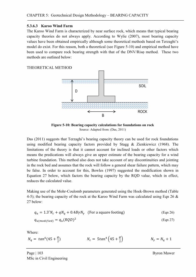
CHAPTER 5: Geotechnical Design Methodology – BEARING CAPACITY
Page | 103 Byron Mawer MSc in Civil Engineering
ROCK B
D SOIL
5.3.6.3 Karoo Wind Farm The Karoo Wind Farm is characterized by near surface rock, which means that typical bearing capacity theories do not always apply. According to Wylie (2007), most bearing capacity values have been obtained empirically although some theoretical methods based on Terzaghi’s model do exist. For this reason, both a theoretical (see Figure 5-10) and empirical method have been used to compare rock bearing strength with that of the DNV/Risφ method. These two methods are outlined below: THEORETICAL METHOD
Figure 5-10: Bearing capacity calculations for foundations on rock Source: Adapted from: (Das, 2011)
Das (2011) suggests that Terzaghi’s bearing capacity theory can be used for rock foundations using modified bearing capacity factors provided by Stagg & Zienkiewicz (1968). The limitations of the theory is that it cannot account for inclined loads or other factors which means the predications will always give an upper estimate of the bearing capacity for a wind turbine foundation. This method also does not take account of any discontinuities and jointing in the rock bed and assumes that the rock will follow a general shear failure pattern, which may be false. In order to account for this, Bowles (1997) suggested the modification shown in Equation 27 below, which factors the bearing capacity by the RQD value, which in effect, reduces the calculated value. Making use of the Mohr-Coulomb parameters generated using the Hoek-Brown method (Table 4-5); the bearing capacity of the rock at the Karoo Wind Farm was calculated using Eqn 26 & 27 below:
𝑞𝑢 = 1.3′𝑁𝑐 + 𝑞𝑁𝑞 + 0.4𝐵𝛾𝑁𝛾 (For a square footing) (Eqn 26)
𝑞𝑢(𝑚𝑜𝑑𝑖𝑓𝑖𝑒𝑑) = 𝑞𝑢(𝑅𝑄𝐷)2 (Eqn 27) Where:
𝑁𝑞 = 𝑡𝑎𝑛6(45 +𝜑
2) 𝑁𝑐 = 5𝑡𝑎𝑛4 (45 +
𝜑
2) 𝑁𝛾 = 𝑁𝑞 + 1

CHAPTER 5: Geotechnical Design Methodology – BEARING CAPACITY
Page | 104 Byron Mawer MSc in Civil Engineering
Under certain conditions, such as when an intact rock possess an inherently high shear strength and additionally when there is a good rock quality designation, the Stagg & Zienkiewicz theory can predict values of much greater than 30 MPa (generally accepted as the compressive strength of concrete). When this value is exceeded, understandably, 30 MPa is then adopted as the ultimate bearing capacity of the rock layer. The results for three drilled boreholes from the Karoo Wind Farm are provided in Table 5-23 with Borehole 1, 4.8m depth being used for comparison across all methods of calculation.
Table 5-23: Results of bearing capacity calculations using Stagg & Zienkiewicz method
POSITION DEPTH (m) Nq Nc Nγ qu (MPa ) RQD (%) qu (modified) qall (MPa )
BH1.1 2.51 4 12 5 18.1 100 18.1 6.0
BH1.2 4.82 15 31 16 115.3 32 11.8 3.9
BH1.3 7.22 50 68 51 405.2 58 136.3 45.4
BH2.1 2.16 3 9 4 9.6 45 1.9 0.6
BH2.2 5.17 8 20 9 55.0 34 6.4 2.1
BH2.3 9.95 23 40 24 186.4 69 88.7 29.6
BH3.1 3.22 4 12 5 23.5 32 2.4 0.8
BH3.2 7.07 14 30 15 147.8 27 10.8 3.6
BH3.3 14.32 47 65 48 521.0 100 521.0 173.7
*FOS of 3 has been applied Since qall is greater than 30 MPa for B1.3 and BH3.3, 30 MPa would be used instead of the value stated in Table 5-23 above. It should also be noted that BH1 is comprised of a sandstone medium, BH2 consists of mudstone and BH3 is dominated by dolerite. The properties and values of each borehole were obtained using the Hoek-Brown method and have been discussed in Section 4.3.3. EMPERICAL METHOD There is a large amount of empirical bearing strength data available, which has been obtained through observation of rock behaviour under loading over the last century. Chapters from Bowles (1997) and Wylie (1999) provide numerous presumed values for a wide variety of rock types and conditions. The problem with using presumed values is that the rock being considered in design may not present the same properties as that investigated by the authors, even if being of the same type or existing in the same conditions. For this reason, empirical relationships based on this data have been developed in order to predict rock-bearing failures. One of these methods outlined in Appendix G of Eurocode 7 based on BS8004, provides values of presumed bearing capacity based on the UCS and degree of jointing evident in the rock bed. This method provides four separate graphs depending on the category that the bedrock falls into (Table 5-24), of which the presumed bearing capacity can be read. The limitations of using this method is that the values are only valid for weak or broken rocks that have not had their

CHAPTER 5: Geotechnical Design Methodology – BEARING CAPACITY
Page | 105 Byron Mawer MSc in Civil Engineering
joints infilled and that the proposed structure can tolerate settlements of not more than 0.5% of the foundation width (90mm for 18m diameter foundation). It is assumed that medium to strong rocks will have bearing capacities greater than 30 MPa making the bearing strength of the rock irrelevant. The method is outlined below:
Table 5-24: Groupings of weak and broken rocks Source: (Eurocode 7, 1997)
GROUP TYPE OF ROCK
1 Pure limestones and dolomites Carbonate sandstones of low porosity
2
Igneous Oolitic and marly limestones Well cemented sandstones Indurated carbonate mudstones Metamorphic rocks, including slates and schist (flat cleavage/foliation)
3 Very marly limestones Poorly cemented sandstones Slates and schists (steep cleavage/foliation)
4 Uncemented mudstones and shales
In the case of Borehole 1, which is dominated by well-cemented sandstones, the description falls into the Group 2 rock category. From this, the Group 2 rock graph (seen in Figure 5-11) can be used to assess bearing resistance. Using this graph, and assumptions surrounding rock joint spacing (Table 5-25) from the borehole logs provided for the Karoo site, the bearing resistances were calculated at each investigation depth in the three boreholes conducted on site:
Table 5-25: Results of bearing capacity calculations using Eurocode 7 empirical method
UCS (MPa)
POSITION DEPTH (m) qu (MPa) ds qullt (MPa)
BH1 2.51 4.0 widely 2
BH1 4.82 70.0 medium 10
BH1 7.22 140.0 closely 30+
BH2 2.16 9.0 widely 9
BH2 5.17 58.0 medium 30+
BH2 9.95 135.0 closely 30+
BH3 3.22 51.6 closely 8
BH3 7.07 146.0 medium 30+
BH3 14.32 92.1 closely 20

CHAPTER 5: Geotechnical Design Methodology – BEARING CAPACITY
Page | 106 Byron Mawer MSc in Civil Engineering
Figure 5-11: Graph showing bearing capacity values for Group 2 rocks Source: (Eurocode 7, 1997)
As qu values were not always at the intervals shown on the figure, or alternatively were greater than 100 MPa, a number of assumptions were made in order to generate a realistic bearing capacity value. These included the following assumptions:
- When qu values fell between graphed lines, the resulting bearing capacity was linearly interpolated from graph figure,
- When qu was greater than 100 MPa, the limiting value of 30 MPa was assumed for design,
- If joints are tight, ultimate bearing pressure cannot exceed uniaxial compressive strength of the rock or 50 % of this value if joints are open. (Eurocode 7, 1997)
- As discontinuity spacing’s are not quantified, bearing pressure values were obtained in the middle of either the f), g), or h) range as per the classification in Table 5-25,
- f) is the closely spaced discontinuity range, - g) is the medium spaced discontinuity range, - h) is the widely spaced discontinuity range, and - A FOS of 3.0 is applied to values to obtain allowable bearing capacities. - After applying the factor of safety to the values obtained and comparing them to the
pressures experienced under the base, the results in Table 5-26 were obtained.

CHAPTER 5: Geotechnical Design Methodology – BEARING CAPACITY
Page | 107 Byron Mawer MSc in Civil Engineering
Table 5-26: Allowable bearing capacity values compared with actual applied pressures
POSITION qu (MPa) qall (MPa ) qact (MPa ) FOS 3
BH1 2 0.67 PASS BH1 10 3.33 PASS BH1 30 10.00 PASS
ROUND SQUARE
BH2 9 3.00 PASS qact (kPa ) qact (kPa )
BH2 30 10.00 PASS LC 1 362.88 283.04
BH2 30 10.00 PASS LC 2 482.48 436.87
BH3 8 2.67 PASS LC 3 278.77 190.39
BH3 30 10.00 PASS
BH3 20 6.67 PASS
5.3.7 Discussion With the completion of the bearing capacity calculations, there is a need to critically compare the results and ultimately choose a value that can be used in design. Typically, the solution that gives the most critical or lowest bearing capacity generated from the worst design case is used for design. As the theories used for each site differed based on underlying assumptions surrounding the make-up of the soil profile, the relative merits and demerits of using this method for choosing a design value needs to be discussed. This discussion is presented for each site before a summary and comparison of all design cases is presented.
5.3.7.1 Eastern Cape Wind Farm The Eastern Cape Wind Farm had generally very favourable shear strength parameters, which is indicative of good bearing capacities. The DNV/Risφ (2002) method in this case (see Table 5-15 & 5-16) gave the most critical theoretical bearing capacity value for both the square and circular footing of 1130 and 1190 kPa respectively with, the higher value for circular footings inherent from the greater effective area that it possesses (Table 5-27 & 5-28). When comparing this to the actual max-applied pressure of 300 kPa, this would seem a very conservative design. However, in this case, the DPSH empirical based bearing capacity of 320 kPa in fact governed the choice in dimensions. This is a far lower value than the theoretical predictions, and is possibly a result of the thin calcrete lenses that exist in the soil bed that can trap weaker soil between them resulting in far lower bearing capacities (Beales, 2015). When comparing results with the rigid base theory in Section 5.3.6.1, it is clear that founding on soils with calcrete beds can potentially reinforce or make the soil weaker depending on the type and extent of pedocrete formation that exists. This is why great care is required when using theoretical methods to predict bearing capacity in these types of soil. For this reason, problems encountered when founding on pedocretes are addressed in Section 5.8.1

CHAPTER 5: Geotechnical Design Methodology – BEARING CAPACITY
Page | 108 Byron Mawer MSc in Civil Engineering
Table 5-27: Summary of design dimensions for Eastern Cape Wind Farm footings
SQAURE CIRCULAR
LC 2 - CRITICAL LC 2 - CRITICAL
B (m) 21 D (m) 21
L (m) 21 df (m) 3
Aeff (m) 266.1 Beff (m) 15.1
Beff (m) 16.31 Leff (m) 18.0
Leff (m) 16.31 Aeff (m2) 271.7
Table 5-28: Summary of bearing capacity results for Eastern Cape Wind Farm footings
SQUARE (qall (kPa)) CIRCULAR (qall (kPa))
DNV/Risφ Bowles Rigid Base qact DNV/Risφ Bowles qact DPSH
LC 1 1220 1450 3400 162 1240 1440 253 320
LC 2 1130 1370 3400 215 1190 1390 300 320
LC 3 1270 1500 3400 125 1270 1470 216 320
5.3.7.2 Western Cape Wind Farm The Western Cape Wind Farm had generally less favourable shear strength parameters than what was found on the Eastern Cape Wind Farm. The DNV/Risφ (2002) method in this case (see Table 5-18) gave the most critical theoretical bearing capacity value for both the square and circular footing of 310 and 350 kPa respectively. This prediction is far closer to that of the DPSH empirical estimate of 250 kPa, which was the most critical for design. An argument must be made however, for the strong soil underlying weak soil case as all bearing capacity DNV/Risφ results are based on the weaker soil shear strength parameters. In order to be conservative, design is based on the most critical value of 250 kPa, however if loading conditions had to increase; the resulting cost to the client would be high in order to redesign. In this case, it may be safe to assume that the bearing capacity is quite possibly higher than that predicted by the DPSH and DNV/Risφ theories. This would need to be assessed and approved however by a qualified geotechnical engineer who is familiar with the ground conditions of the area in question. To account for these ground conditions, a square footing of 21 x 21m or a circular footing of 23m diameter would be required in order to provide a safe bearing capacity to resist the applied loads of 215 and 236 kPa respectively. Table 5-29 and 5-30 show a summary of the design dimensions and bearing capacity results for the Western Cape Wind Farm.

CHAPTER 5: Geotechnical Design Methodology – BEARING CAPACITY
Page | 109 Byron Mawer MSc in Civil Engineering
Table 5-29: Summary of design dimensions for Western Cape Wind Farm footings SQAURE CIRCULAR
LC 2 - CRITICAL LC 2 - CRITICAL
B (m) 21 D (m) 23
L (m) 21 df (m) 3
Aeff (m) 266.1 Beff (m) 17.0
Beff (m) 16.31 Leff (m) 19.78
Leff (m) 16.31 Aeff (m2) 336.0
Table 5-30: Summary of bearing capacity results for Western Cape Wind Farm footings
SQUARE (qall (kPa)) CIRCULAR (qall (kPa))
DNV/Risφ Bowles SUW qact DNV/Risφ Bowles qact DPSH
LC 1 340 380 441 162 370 400 203 250
LC 2 310 360 416 215 350 390 236 250
LC 3 350 400 455 125 370 410 176 250
5.3.7.3 Karoo Wind Farm It has already been discussed how according to Wylie (1999), since the Karoo Wind Farm is founded upon rock, that the bearing capacity is generally not the most critical criteria of foundation design. For this reason, theoretical bearing capacity theories such as the DNV/Risφ method, as well as the modification applied for the Bowles factors, offer extremely high bearing resistances based on the input c’ and φ’ values obtained using the Hoek – Brown method. Compared to the Stagg & Zienkiewicz (1968) and Eurocode 7 method that have been developed specifically for founding on rocks, it is possible that these theories can be more representative estimations of the rock’s allowable bearing strength. As the Eurocode 7 method is the most critical in this case, this value is used for the design. This being stated, the closest applied pressure to this prediction is still 7 times smaller than that of the 3330 kPa capacity. As the DPSH or any other probe method will often refuse on such a hard material as rock, no empirical investigation based approximations of strength are available for comparison. In this case, therefore the foundation dimensions were optimized at 18 x 18m for a square footing and 18m in diameter for a circular footing in order to resist max-applied pressures of 437 and 482 kPa respectively. Table 5-31 and 5-32 show a summary of the design dimensions and bearing capacity results for the Karoo Wind Farm.
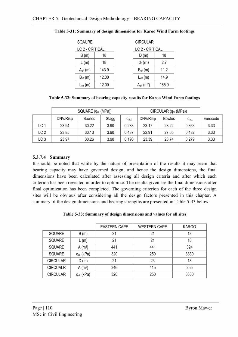
CHAPTER 5: Geotechnical Design Methodology – BEARING CAPACITY
Page | 110 Byron Mawer MSc in Civil Engineering
Table 5-31: Summary of design dimensions for Karoo Wind Farm footings SQAURE
CIRCULAR
LC 2 - CRITICAL
LC 2 - CRITICAL
B (m) 18
D (m) 18
L (m) 18
df (m) 2.7
Aeff (m) 143.9
Beff (m) 11.2
Beff (m) 12.00
Leff (m) 14.9
Leff (m) 12.00
Aeff (m2) 165.9
Table 5-32: Summary of bearing capacity results for Karoo Wind Farm footings
SQUARE (qall (MPa)) CIRCULAR (qall (MPa))
DNV/Risφ Bowles Stagg qact DNV/Risφ Bowles qact Eurocode
LC 1 23.94 30.22 3.90 0.283 23.17 28.22 0.363 3.33
LC 2 23.85 30.13 3.90 0.437 22.91 27.65 0.482 3.33
LC 3 23.97 30.26 3.90 0.190 23.39 28.74 0.279 3.33
5.3.7.4 Summary It should be noted that while by the nature of presentation of the results it may seem that bearing capacity may have governed design, and hence the design dimensions, the final dimensions have been calculated after assessing all design criteria and after which each criterion has been revisited in order to optimize. The results given are the final dimensions after final optimization has been completed. The governing criterion for each of the three design sites will be obvious after considering all the design factors presented in this chapter. A summary of the design dimensions and bearing strengths are presented in Table 5-33 below:
Table 5-33: Summary of design dimensions and values for all sites
EASTERN CAPE WESTERN CAPE KAROO
SQUARE B (m) 21 21 18
SQUARE L (m) 21 21 18
SQUARE A (m2) 441 441 324
SQUARE qall (kPa) 320 250 3330
CIRCULAR D (m) 21 23 18
CIRCUALR A (m2) 346 415 255
CIRCULAR qall (kPa) 320 250 3330
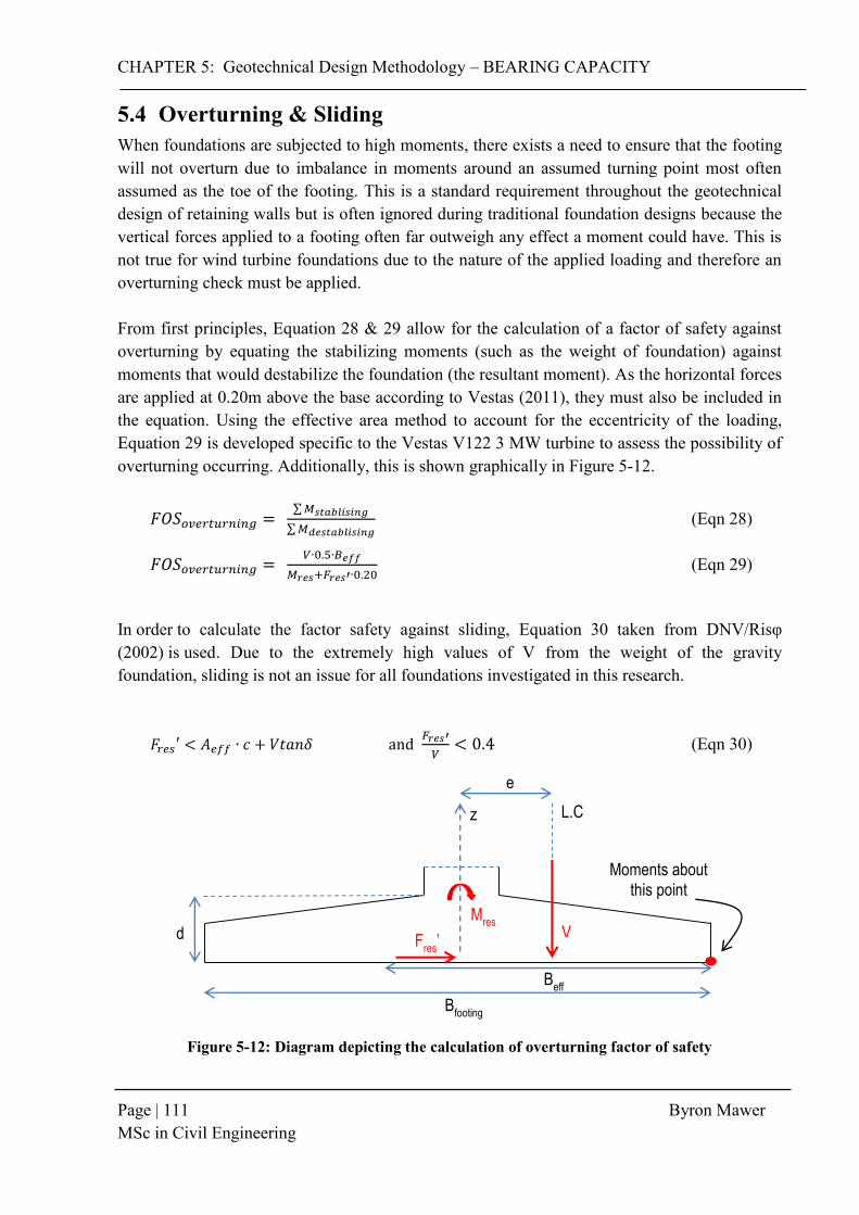
CHAPTER 5: Geotechnical Design Methodology – BEARING CAPACITY
Page | 111 Byron Mawer MSc in Civil Engineering
Bfooting
d V F
res’
Mres
e
z L.C
Beff
Moments about this point
5.4 Overturning & Sliding When foundations are subjected to high moments, there exists a need to ensure that the footing will not overturn due to imbalance in moments around an assumed turning point most often assumed as the toe of the footing. This is a standard requirement throughout the geotechnical design of retaining walls but is often ignored during traditional foundation designs because the vertical forces applied to a footing often far outweigh any effect a moment could have. This is not true for wind turbine foundations due to the nature of the applied loading and therefore an overturning check must be applied. From first principles, Equation 28 & 29 allow for the calculation of a factor of safety against overturning by equating the stabilizing moments (such as the weight of foundation) against moments that would destabilize the foundation (the resultant moment). As the horizontal forces are applied at 0.20m above the base according to Vestas (2011), they must also be included in the equation. Using the effective area method to account for the eccentricity of the loading, Equation 29 is developed specific to the Vestas V122 3 MW turbine to assess the possibility of overturning occurring. Additionally, this is shown graphically in Figure 5-12.
𝐹𝑂𝑆𝑜𝑣𝑒𝑟𝑡𝑢𝑟𝑛𝑖𝑛𝑔 = ∑ 𝑀𝑠𝑡𝑎𝑏𝑙𝑖𝑠𝑖𝑛𝑔
∑ 𝑀𝑑𝑒𝑠𝑡𝑎𝑏𝑙𝑖𝑠𝑖𝑛𝑔 (Eqn 28)
𝐹𝑂𝑆𝑜𝑣𝑒𝑟𝑡𝑢𝑟𝑛𝑖𝑛𝑔 = 𝑉∙0.5∙𝐵𝑒𝑓𝑓
𝑀𝑟𝑒𝑠+𝐹𝑟𝑒𝑠′∙0.20 (Eqn 29)
In order to calculate the factor safety against sliding, Equation 30 taken from DNV/Risφ (2002) is used . Due to the extremely high values of V from the weight of the gravity foundation, sliding is not an issue for all foundations investigated in this research.
𝐹𝑟𝑒𝑠′ < 𝐴𝑒𝑓𝑓 ∙ 𝑐 + 𝑉𝑡𝑎𝑛𝛿 and 𝐹𝑟𝑒𝑠′
𝑉< 0.4 (Eqn 30)
Figure 5-12: Diagram depicting the calculation of overturning factor of safety

CHAPTER 5: Geotechnical Design Methodology – BEARING CAPACITY
Page | 112 Byron Mawer MSc in Civil Engineering
The overturning and sliding checks were conducted on all three wind turbine designs for each of the case studies addressed in this research. This is where the major advantage of using circular foundations is highlighted as it not only uses up less area, but also inherently has a far higher volume due to the nature of its shape, which imparts a far higher vertical gravity load into the soil. In comparison therefore, the circular foundation will have a higher factor of safety against overturning than the square footing. Consulting Table 5-34 & 5-35 below, as the Eastern Cape and Western Cape wind farms were governed more by bearing capacity and gapping, the factor of safety against overturning and the factor of safety against sliding are reasonably high. For the Karoo Wind Farm however (see Table 5-36), using only gapping as the critical design factor, the factor of safety against overturning is below the desired 2.0 for the square footings and only just above 2.0 for the circular footing. This additionally emphasizes the importance of designing for 0% gapping, as it can help maintain a sufficient FOS against overturning. Due to the ability of circular foundations ability to have a higher resistance to overturning, these foundations have been carried through in the rest of the design.
Table 5-34: Results of Overturning and Sliding checks for Eastern Cape Wind Farm
OVERTURNING
Square: Scenario 1 Square : Scenario 2 Circular
V (kN) Mres (kNm) FOS V (kN) Mres (kNm) FOS V (kN) Mres (kNm) FOS
LC 1 25758.0 66700 3.05 25758.0 66700 3.34 47736.6 66700 5.67
LC 2 25668.0 85100 2.16 25668.0 85100 2.45 47646.6 85100 4.22
LC 3 25788.0 49100 4.50 25788.0 49100 4.80 47766.6 49100 8.04
SLIDING
Square: Scenario 1 Square : Scenario 2 Circular
Fres' Resistance FOS Fres' Resistance FOS Fres' Resistance FOS
LC 1 729.4 13874 19 736.9 13495 18 735.0 21779 30
LC 2 1189.2 13474 11 1238.6 13046 11 1218.1 21550 18
LC 3 628.0 14231 23 639.6 13921 22 639.7 21975 34
Table 5-35: Results of Overturning and Sliding checks for Western Cape Wind Farm
OVERTURNING
Square: Scenario 1 Square : Scenario 2 Circular
V (kN) Mres (kNm) FOS V (kN) Mres (kNm) FOS V (kN) Mres (kNm) FOS
LC 1 25758.0 66700 3.05 25758.0 66700 3.34 49157.9 66700 6.51
LC 2 25668.0 85100 2.16 25668.0 85100 2.45 49067.9 85100 4.88
LC 3 25788.0 49100 4.50 25788.0 49100 4.80 49187.9 49100 9.20
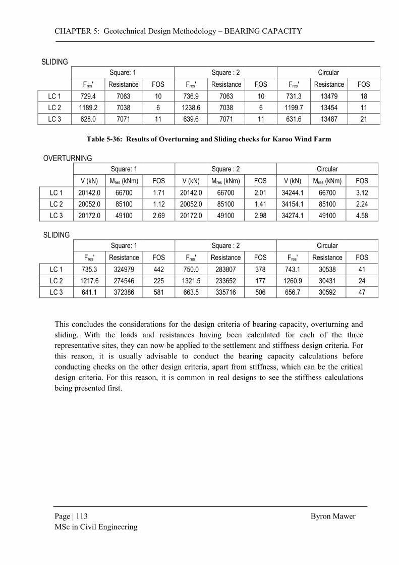
CHAPTER 5: Geotechnical Design Methodology – BEARING CAPACITY
Page | 113 Byron Mawer MSc in Civil Engineering
SLIDING
Square: 1 Square : 2 Circular
Fres' Resistance FOS Fres' Resistance FOS Fres' Resistance FOS
LC 1 729.4 7063 10 736.9 7063 10 731.3 13479 18
LC 2 1189.2 7038 6 1238.6 7038 6 1199.7 13454 11
LC 3 628.0 7071 11 639.6 7071 11 631.6 13487 21
Table 5-36: Results of Overturning and Sliding checks for Karoo Wind Farm
OVERTURNING
Square: 1 Square : 2 Circular
V (kN) Mres (kNm) FOS V (kN) Mres (kNm) FOS V (kN) Mres (kNm) FOS
LC 1 20142.0 66700 1.71 20142.0 66700 2.01 34244.1 66700 3.12
LC 2 20052.0 85100 1.12 20052.0 85100 1.41 34154.1 85100 2.24
LC 3 20172.0 49100 2.69 20172.0 49100 2.98 34274.1 49100 4.58
SLIDING
Square: 1 Square : 2 Circular
Fres' Resistance FOS Fres' Resistance FOS Fres' Resistance FOS
LC 1 735.3 324979 442 750.0 283807 378 743.1 30538 41
LC 2 1217.6 274546 225 1321.5 233652 177 1260.9 30431 24
LC 3 641.1 372386 581 663.5 335716 506 656.7 30592 47
This concludes the considerations for the design criteria of bearing capacity, overturning and sliding. With the loads and resistances having been calculated for each of the three representative sites, they can now be applied to the settlement and stiffness design criteria. For this reason, it is usually advisable to conduct the bearing capacity calculations before conducting checks on the other design criteria, apart from stiffness, which can be the critical design criteria. For this reason, it is common in real designs to see the stiffness calculations being presented first.

CHAPTER 5: Geotechnical Design Methodology – SETTLEMENT
Page | 114 Byron Mawer MSc in Civil Engineering
5.5 Settlement 5.5.1 Introduction Settlement is defined as the downward movement of soil due to an increase in vertical strain in the soil, caused by an increase in vertical stress. The increase in vertical stress is most often associated with an applied loading, which in this case, is the loading applied by wind turbine foundation that is constructed on the soil or rock mass. According to Das (2011), the design of foundations of small breadth are generally governed by bearing capacity, but as breadth increases, the considerations of allowable settlement begins to slowly dominate the design. As wind turbines are often no less than 15m in diameter, it is a reasonable assumption that settlement may be a limiting factor for design. Settlement also occurs in a number of different phases or under different mechanisms and can be estimated using Equation 31 sourced from Das (2011):
𝑆𝑇 = 𝑆𝑒 + 𝑆𝑐 + 𝑆𝑠 (Eqn 31) Where: ST = the total settlement experienced below a foundation, Se = the immediate elastic settlement, Sc = the primary consolidation settlement, and
Ss = the secondary consolidation settlement, According to Das (2011) and Craig (2004), for any foundation being analysed, one or more of the components of the above total settlement equation may be zero or negligible depending on the prevalent conditions on site, primarily the type of soil and ground water conditions. The conditions for which each of the elements of total settlement applies include:
- Elastic settlement: Generally caused by the immediate deformation of dry, moist or saturated soils under load, assuming an elastic stress-strain relationship, without any change in moisture content.
- Primary consolidation: Occurs generally in submerged fine-grained clayey soils due to the expulsion of pore-pressures over time, as the pore water in the void spaces attempts to move to areas of lower pressure. This generally is a slow process and occurs over decades depending on the permeability of the soil.
- Secondary consolidation: This generally occurs after the primary consolidation stage and is a result of the plastic adjustment of soil fabrics. This often occurs in organic soils as the organic components are broken down.
In this study, none of the soil profiles exhibited a water table and none was found to hold any significant organic content. For this reason, only immediate elastic settlement was investigated. For fine-grained soils that are organic or submerged, the additional settlement due to consolidation would need to be investigated.

CHAPTER 5: Geotechnical Design Methodology – SETTLEMENT
Page | 115 Byron Mawer MSc in Civil Engineering
Settlement is generally considered one of the harder soil design parameters to predict and estimates are often based on semi-empirical methods developed for a specific type of soil. For wind turbine foundations, which are subject to a number of low strain dynamic load cycles throughout their lifetime, this becomes an even more complex problem. In South Africa, settlement predictions are usually based on local experience coupled with empirical correlations with SPT or other probe test results. This is then compared to the traditional elastic settlement equation results in order to generate an approximation of the expected settlement that will be experienced by the footing. Additionally to this, computer software that calculate settlement based on elastic theory, such as Rocscience’s Settle 3D or Finite Element Modelling is also commonly used, each with their own set of limitations. The advantage of settlement calculations for a wind turbine site is the fact that CSW tests are conducted for stiffness checks, allowing for a precise value of the in-situ soil stiffness (E) to be calculated. This value is very often assumed during traditional foundation design leading to settlement predictions that are limited by the accuracy of this estimation. While the availability of this data is an advantage, due to the low strain dynamic load cycles experienced by the turbine from the rotation of the rotor blade, the soil undergoes stiffness degradation with time. In order to account for this, Archer (2014) suggested the use of a non-linear step wise settlement prediction method that not only accounts for stiffness degradation with increasing soil strain under loading, but also accounts for the non-linear behaviour of soil while still allowing a estimate based in elastic theory. The applicability of this method was proved by comparing forecasts of the method with the results of centrifuge testing conducted on South African sands at the University of Pretoria. As it is often easier to use theoretical methods during design, it was decided for the purposes of this study, to use three theoretical models to calculate settlement including the traditional elastic settlement method commonly used in South Africa, predictions of the settlement software Settle 3D and finally, the Archer (2014) Non-Linear Step Wise method. The results of each method for the three representative sites are compared and discussed in order to ascertain a reasonable design value for settlement.
5.5.2 Foundation Rigidity & Stress Distribution As settlement is directly related to the change of vertical stress in a soil body, before any predictions of soil settlement can be addressed, a method of predicting stress and strain at a certain point in a soil mass must be discussed. Foundation rigidity relative to the soil also contributes to the distribution of stress across the foundation breadth and therefore, at what point along the foundation the maximum settlement will occur. A foundation is classified as either rigid or flexible depending on the way it tends to deform under load. It can be seen that for flexible footing in a cohesive soil (Figure 5-13a), the footing deforms with the applied loading, allowing for the maximum strain and therefore settlement to

CHAPTER 5: Geotechnical Design Methodology – SETTLEMENT
Page | 116 Byron Mawer MSc in Civil Engineering
a) b)
c) d)
occur in the middle of the footing. For 5-13b) a flexible footing in a granular soil, the soil at the centre is confined which results in that area exhibiting a higher modulus of elasticity. As the contact pressure is constant across the footing, the edges of footing experience a larger strain under the same pressure than at the centre and therefore a larger settlement is experienced at the edges of the footing. For rigid footings, settlement is expected to be uniform as differential settlement is limited due to the stiffness of the footing. For 5-13c) a rigid footing on a cohesive soil, the contact pressure is smaller at the centre and a maximum at the edges. Alternatively, for 5-13d) a rigid footing on a granular soil, the opposite trend is observed. A number of factors contribute to whether a foundation is considered flexible or rigid including soil stiffness, structural stiffness and foundation geometry however, according to Bowles (1997); it has been found that in practice a linear distribution approximation is adequate to predict foundation behaviour, as the majority of stress distributions under footings are in fact indeterminate. For this reason, a linear approximation has been used for the purposes of this design. The problem with this assumption is that, the Settle 3D software used to analyse settlement requires the input of a choice of foundation rigidity. For these purposes, the foundation was assumed flexible, in line with the theory of elastic settlement used in the traditional method. Additionally, foundations subjected to low frequency dynamic loads are often designed to be flexible in order to avoid repetitive uplift from the ground through load cycles. With a stiff footing, this repetitive hammering on the soil would cause a compactive effect, which can degrade the soil over time. This assumption also generally gives a more conservative estimation of soil pressures and hence is favoured by designers (Beales, 2015).
Figure 5-13: Effect of contact pressure on settlement distribution – a) flexible footing on cohesive soil, b) flexible footing on granular soil, c) rigid footing on cohesive soil, and d) rigid footing on
granular footing. Source: Adapted from: (Kalumba, 2015)

CHAPTER 5: Geotechnical Design Methodology – SETTLEMENT
Page | 117 Byron Mawer MSc in Civil Engineering
While foundation rigidity has a notable effect on the contact stress experienced between footing and the soil, it does not predict the way in which stress (and therefore strain) will be distributed from the bottom of the footing into the soil bed to depth. In order to quantify this distribution, a number of mathematical relationships between loads applied to a soil and the stress experienced at any point below the footing have been developed. The most commonly used model is that developed by Boussinesq although other models such as Westergaard, Newmark, Fröhlich and the Poulos & Davis method have all been developed to address certain problems or to increase ease of calculation. In order to tie in with the assumptions of the settlement theories selected for analysis, the Boussinesq theory is used for this study. Boussinesq’s mathematical relationship was initially developed in order to account for a point load, but has since been expanded to deal with various types of loading including uniformly distributed loads under square and circular footings. Making use of Figure 5-14, a circular area of radius R, under a uniform pressure q (assumed as worst-case value distributed evenly across foundation width), allows the vertical stress increase to be calculated (Equation 32). This formulation can be extended to calculate the radial or lateral stress using Equation 33.
𝜎𝑧 = 𝑞[1 − (1
1+(𝑅 𝑧)⁄ 2)3/2] (Eqn 32)
𝜎𝑟 =𝑞
2[(1 + 2𝑣) −
2(1+𝑣)
√1+(𝑅 𝑧⁄ )2+
1
[1+(𝑅 𝑧)⁄ 2]3
2⁄] (Eqn 33)
Figure 5-14: Stress distribution at a point under circular distributed load Source: (Das, 2011)

CHAPTER 5: Geotechnical Design Methodology – SETTLEMENT
Page | 118 Byron Mawer MSc in Civil Engineering
5.5.3 Traditional Elastic Solution for Settlement of Foundation A number of texts including those of Das (2011), Bowles (1997) and Craig (2004) all refer to the calculation of settlement under a footing by making use of the elastic theory. As settlement is directly related to the level of strain in the soil, this is calculated simply by integrating the level of strain experienced throughout the soil by assuming that stress is directly proportional to strain through the modulus of elasticity. (See derivation in Equation 34 below).
𝑆𝑒 = ∫ 휀𝑧𝑑𝑧𝐻
0=
1
𝐸𝑠∫ (∆𝜎𝑧 − 𝑣∆𝜎𝑥 − 𝑣∆𝜎𝑦)𝑑𝑧
𝐻
0 (Eqn 34)
This was then simplified by Bowles (1997) into Equation 35 below which relates the total expected settlement to the load applied, the breadth of the footing, the modulus of elasticity, the Poisson’s ratio for the soil and an influence factor dependent on foundation geometry and rigidity. The influence factor is generally obtained from tables made available by Bowles (1997), recreated in Table 5-37 below.
𝑆𝑒 =𝑞𝐵
𝐸(1 − 𝑣2)𝐼𝑓 (Eqn 35)
Table 5-37: Influence Factor (If) for rigid and flexible foundations
Source: (Bowles, 1997)
Shape Flexible Foundation Rigid Foundation
Center Corner Average
Circular 1.00 0.64 0.85 0.86
Square 1.12 0.56 0.95 0.82
Rectangle
L/B = 1.5 1.36 0.68 1.20 1.06
L/B = 2 1.52 0.76 1.30 1.20
L/B = 5 2.10 1.05 1.83 1.70
L/B = 10 2.52 1.26 2.25 2.10
L/B = 100 3.38 1.69 2.96 3.40
As all foundations have been assumed flexible with an assumed linear distribution of pressure, the maximum settlement should occur beneath the centre of the footing. For this reason, an If value of 1.0 is chosen for the settlement calculations for each site. The limitation of this method is that an average value of E must be used for a depth between 1.5 and 2 times the breadth of the footing. If the soils at depth are very strong or are rock for example, with a high Es value, this can increase the average E to a value far greater than that of the weaker soils directly beneath the footing. This ultimately provides an estimation of settlement far smaller than what will actually be experienced.

CHAPTER 5: Geotechnical Design Methodology – SETTLEMENT
Page | 119 Byron Mawer MSc in Civil Engineering
For each of the three sites being investigated, the elastic solution for settlement has been explored and quantified. The results of which are given below: EASTERN CAPE WIND FARM After applying the If equal to 1.00 from Table 5-37, the elastic settlement equation is given as: 𝑆𝑒 =
𝑞𝐵
𝐸(1 − 𝑣2)
Before the calculation can be attempted, an average value of Es for the soil must first be attained. Generally, an Es value is assumed from literature, however since results of CSW testing are available, these values can be used for the calculation of settlement. The reduction of G0 from the CSW tests into E0 as well as the reduction of E0 into an E applicable for the strain range experienced is covered in Section 5.7 when dealing with foundation stiffness, however the calculated E values experienced across the soil profile at each relevant depth is summarized in Table 5-38 below. The Eavg is calculated using a weighted average where the E value is weighted by the contribution it makes to the soil profile. This is achieved by summing the product of each E value and the thickness of the appropriate layer and dividing it by the total thickness of the soil profile. The value for v was assumed from the description of the soil profile presented in Section 4.3.
Table 5-38: Summary of E values over Eastern Cape Wind Farm soil profile
Go (MPa) Eo (MPa) E (MPa) ν
3m - 5m 345 897 711 0.3
5m - 7m 355 923 732 0.3
7m - 9m 360 936 742 0.3
9m -11m 365 949 753 0.3
11m - 13m 370 962 763 0.3
13m - 15m 370 962 763 0.3
AVG: 744
Using the following parameters for the Eastern Cape Wind Farm:
q = 216 kPa B = 21 m E = 744 MPa 𝑆𝑒 =
𝑞𝐵
𝐸(1 − 𝑣2)
∴ 𝑆𝑒 =216×21
744(1 − 0.32)
∴ 𝑆𝑒 = 𝟓. 𝟓𝟓 𝒎𝒎 Over 30m profile.
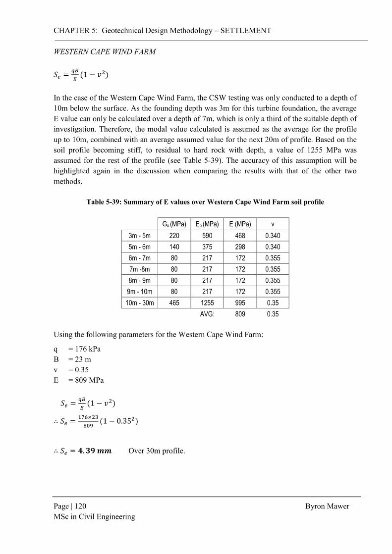
CHAPTER 5: Geotechnical Design Methodology – SETTLEMENT
Page | 120 Byron Mawer MSc in Civil Engineering
WESTERN CAPE WIND FARM 𝑆𝑒 =
𝑞𝐵
𝐸(1 − 𝑣2)
In the case of the Western Cape Wind Farm, the CSW testing was only conducted to a depth of 10m below the surface. As the founding depth was 3m for this turbine foundation, the average E value can only be calculated over a depth of 7m, which is only a third of the suitable depth of investigation. Therefore, the modal value calculated is assumed as the average for the profile up to 10m, combined with an average assumed value for the next 20m of profile. Based on the soil profile becoming stiff, to residual to hard rock with depth, a value of 1255 MPa was assumed for the rest of the profile (see Table 5-39). The accuracy of this assumption will be highlighted again in the discussion when comparing the results with that of the other two methods.
Table 5-39: Summary of E values over Western Cape Wind Farm soil profile
Go (MPa) Eo (MPa) E (MPa) ν
3m - 5m 220 590 468 0.340
5m - 6m 140 375 298 0.340
6m - 7m 80 217 172 0.355
7m -8m 80 217 172 0.355
8m - 9m 80 217 172 0.355
9m - 10m 80 217 172 0.355
10m - 30m 465 1255 995 0.35
AVG: 809 0.35
Using the following parameters for the Western Cape Wind Farm:
q = 176 kPa B = 23 m v = 0.35 E = 809 MPa 𝑆𝑒 =
𝑞𝐵
𝐸(1 − 𝑣2)
∴ 𝑆𝑒 =176×23
809(1 − 0.352)
∴ 𝑆𝑒 = 𝟒. 𝟑𝟗 𝒎𝒎 Over 30m profile.

CHAPTER 5: Geotechnical Design Methodology – SETTLEMENT
Page | 121 Byron Mawer MSc in Civil Engineering
KAROO WIND FARM 𝑆𝑒 =
𝑞𝐵
𝐸(1 − 𝑣2)
For the Karoo Wind Farm, the CSW testing was conducted to a depth of 20m below the ground surface. As the founding depth was 3m for this turbine foundation, the average E value can only be calculated over a depth of 17m. In order to account for this, the next 10m to a depth of 30m is assumed to have the same stiffness parameters as the rock above it. This is because after 9.5m, the borehole log exhibited the same rock material to the end of the profile. It is therefore considered a safe assumption that the rock will generally exhibit the same stiffness properties to depth. After taking into account the applicable strain range of ε = 10-2 for wind turbine loading, the weight averaged E was calculated as 10 390 MPa for the profile (see Table 5-40):
Table 5-40: Summary of E values over Karoo Wind Farm soil profile
Go (MPa) Eo (MPa) E (MPa) ν
1 - 1.5m 363 899 713 0.24
1.5 – 3m 122 314 249 0.29
3 - 4.5m 122 314 249 0.29
4.5 – 7m 2072 5055 4009 0.22
7 - 9.5m 2072 5055 4009 0.22
9.5 – 17m 6667 16000 12689 0.20
17 - 24.5m 6667 16000 12689 0.20
24.5 - 30m 6667 16000 12689 0.20
AVG: 10390 0.22
Using the following parameters for the Karoo Wind Farm:
q = 279 kPa B = 18 m v = 0.22 E = 10390 MPa 𝑆𝑒 =
𝑞𝐵
𝐸(1 − 𝑣2)
∴ 𝑆𝑒 =279×18
10390(1 − 0.222)
∴ 𝑆𝑒 = 𝟎. 𝟒𝟔𝟎 𝒎𝒎 Over 30m profile.

CHAPTER 5: Geotechnical Design Methodology – SETTLEMENT
Page | 122 Byron Mawer MSc in Civil Engineering
5.5.4 Archer (2014) Non-Linear Step Wise Method The main problems with settlement estimation methods used in South Africa are that they are mostly based on empirical SPT relationships or based on local experience. Additionally to this, Archer (2014) explains how it is also convenient to only require one single parameter (in this case E0) in order to predict settlement. This is favoured from relying on soil parameters obtained from laboratory testing as there is always an inherent risk of sample disturbance or other human based errors occurring, which can affect the accuracy of results. Archer therefore advised the use of a non-linear step wise method which has the advantage that it incorporates the stiffness changes with depth and does not assume an average E value for the entire profile as in traditional elastic solution, and it requires no laboratory testing, only in-situ seismic tests in order to obtain the stiffness profile of the soil. For conventional foundations, the argument could be made that traditional settlement calculations have been used for an extended period of time with very few issues. Considering that laboratory testing is required for other design criteria such as bearing capacity, it may be a considered wasteful to spend additional capital on seismic tests that are not needed for any other purpose than to aid in the calculation of settlement. As wind turbine foundations already require seismic testing in order to generate a stiffness profile for foundation stiffness checks, this method becomes an attractive solution as it avoids the possible lab based errors considered above. For this reason, this method has been used and compared with the results of the other settlement prediction methods in order to ascertain its viability for future wind turbine settlement checks. The method involves the following a step by step process presented by Archer (2014): - Obtain the small-strain shear stiffness profile with depth from in-situ seismic methods - Sub-divide the material below the foundation into layers down to at least a depth equalling
twice the foundation width or diameter. - Assign E0 as initial Young’s Modulus for each layer calculated from G0 together with
Poisson’s ratio using Equation 6:
𝐸0 = 2 ∙ 𝐺0(1 + 𝑣) - Decide on the maximum applied stress as well as the number of load steps to be used. - Using Boussinesq’s theory, calculate the vertical stress increment at the centre of each layer
using Equation 32 and the radial stress from Equation 33.
𝜎𝑧 = 𝑞[1 − (1
1+(𝑅 𝑧)⁄ 2)3/2 ]
𝜎𝑟 = 𝜎𝜃 =𝑞
2[(1 + 2𝑣) −
2(1+𝑣)
√1+(𝑅 𝑧⁄ )2+
1
[1+(𝑅 𝑧)⁄ 2]3
2⁄]

CHAPTER 5: Geotechnical Design Methodology – SETTLEMENT
Page | 123 Byron Mawer MSc in Civil Engineering
- Calculate the vertical strain (εv) for the first load step for each layer using Equation 36 which incorporates the vertical (σz) as well as the radial (σr) and circumferential stress (σθ).
휀𝑣 =[𝜎𝑧−2𝑣𝜎𝑟]
𝐸0 (Eqn 36)
- The vertical strain is calculated for the first load step with the use of the small-strain Young’s modulus values.
- Since the strain calculated is axial strain, the values should be transformed to shear strain (εs) for use with the stiffness degradation curves using Equation 37.
휀𝑠 = 휀𝑣 ∙2
3(1 + v) (Eqn 37)
- Using a stiffness degradation curve together with the strain in each layer after application of the first load step, a new Young’s modulus value is calculated for use in the next load step. For this study, a Ramberg & Osgood based stiffness reduction curve was used, obtained from Clayton & Heymann (2001) [see Table 3-2]:
𝐺
𝐺0=
𝐸
𝐸0=
1
[1+16𝛾(1+10−20𝛾)]
- For each load step, the strain is calculated together with a stiffness reduction curve to calculate a new Young’s Modulus (Ei) at each strain value.
- The process is repeated until the maximum applied stress is reached. - The total settlement is the combined settlement for all sub-layers (sub-layer thickness
multiplied by the vertical strain calculated) for all the load steps:
Total Settlement = ∑ LOAD STEPS (∑ H ∙ ε) (Eqn 38) In Archer’s study, the results of this non-linear method were compared with practical tests on sandy soils making use of centrifuge testing which typically gave a range of results based on stresses from 0 to 7000 kPa. The applicability of this method for lower stress of not greater than 500 kPa will be assessed. The process is shown systematically for the Eastern Cape Wind Farm design example, after which, the results for the Western Cape and Karoo Wind Farms are presented: EASTERN CAPE WIND FARM Following the methodology stated above, the first and second step involves outlining the small strain stiffness profile from the CSW testing that was conducted on site. This is presented in Figure 4-11, 13, 15 of Section 4.3.1. The next step is to divide the soil into layers and assign E0 values to each layer. It was decided to follow the soil profile as much as possible, and therefore a 2m layer spacing was used starting from a depth of 3m (the depth of embedment) until the termination depth of the CSW test that was 15m. Using the CSW results, E0 values were obtained from the G0 values recorded and assigned to each layer as highlighted in Table 5-41 below:

CHAPTER 5: Geotechnical Design Methodology – SETTLEMENT
Page | 124 Byron Mawer MSc in Civil Engineering
Table 5-41: Summary of soil layers and assigned E0 value for Eastern Cape Wind Farm
Go (MPa) Eo (MPa) ν
3m - 5m 345 897 0.3
5m - 7m 355 923 0.3
7m - 9m 360 936 0.3
9m -11m 365 949 0.3
11m - 13m 370 962 0.3
13m - 15m 370 962 0.3
With soil layers defined with assigned E0 values, the next step is to decide on the max-applied pressure and the load steps that would be used. It was decided as the turbines are constructed in the sequence: foundation, tower, nacelle and blades, that four load steps would be appropriate. The max applied pressure is assumed to be the bearing pressure applied from the worst load case as calculated in Section 5.3, for the Eastern Cape Wind Farm this value was 216 kPa, which over 4 load steps, was calculated as 54 kPa each. The next step involves calculating the stress and strain distribution in the soil due to the applied loading. This comprises of the vertical, radial and circumferential stresses calculated in the middle of each layer using Equation 32 and 33. These stresses are then combined in order to calculate the axial and shear stresses using the equations shown in the methodology above. A summary of the results for load step 1 are shown in Table 5-42 below. Using the stiffness reduction curve and the calculated shear strain in the soil, the E0 value is then reduced to coincide with the applicable strain range being applied to the soil. As the shear strains are so low (10-5) there is very little to no stiffness reduction in this case: Table 5-42: Summary of calculation of stresses, strains and stiffness reduction for EC Wind Farm
LAYER σz (kPa) σr (kPa) εv εs Enew (MPa)
3m - 5m 53.95 36.57 3.6E-05 3.1E-05 896
5m - 7m 52.88 24.47 4.1E-05 3.6E-05 922
7m - 9m 49.71 15.16 4.3E-05 3.8E-05 935
9m -11m 44.78 8.87 4.2E-05 3.6E-05 948
11m - 13m 39.12 4.96 3.8E-05 3.3E-05 961
13m - 15m 33.56 2.64 3.3E-05 2.9E-05 961
After calculating the new E value, the adapted values are then used in the following load step calculations and the entire process is repeated revising the E value for each load step. With the calculation completed for each load step, the total settlement can be calculated. As the change in E is minimal, and the stress increments for each load step are equal, the total settlement

CHAPTER 5: Geotechnical Design Methodology – SETTLEMENT
Page | 125 Byron Mawer MSc in Civil Engineering
experienced for each load step is the same. Therefore, the total settlement calculated for the first load step in Table 5-43 below is multiplied by 4 in order to calculate the final settlement under the full applied loading. As the profile only extends to 15m, in order to extend it to a range of 30m, the final value obtained was multiplied by 2. As the soil is assumed to maintain a similar or greater stiffness to a depth of 30m based on the soil profile, it is a safe assumption that the settlement that does occur will be less than what is calculated for upper 15m. In order to be conservative, the value was decided to be doubled.
Table 5-43: Summary of calculation of settlement for EC Wind Farm
LAYER Settlement 3m - 5m 0.062 mm
5m - 7m 0.072 mm
7m - 9m 0.075 mm
9m -11m 0.072 mm
11m - 13m 0.065 mm
13m - 15m 0.058 mm
SETTLEMENT
TOTAL: 0.404 mm x 4 LOAD STEPS = 1.61 mm
x 2 =
3.23 mm
It is evident when using this method, that at such low applied stresses, the stiffness reduction is not as marked as when using the traditional elastic solution where a strain of 10-2 is assumed. While this is a potential limitation of this method, it may provide a more accurate answer as the stiffness profile is not averaged over the area of investigation as in the traditional method. For the Western Cape and Karoo wind farms, the results of using the Archer (2014) method are highlighted in the series of tables (5-44, 5-45) below: WESTERN CAPE WIND FARM
Table 5-44.1: Summary of results of Archer (2014) stress-strain calcs for WC site
Go (MPa) Eo (MPa) ν
3m - 5m 220 590 0.340
5m - 6m 140 375 0.340
6m - 7m 80 217 0.355
7m -8m 80 217 0.355
8m - 9m 80 217 0.355
9m - 10m 80 217 0.355

CHAPTER 5: Geotechnical Design Methodology – SETTLEMENT
Page | 126 Byron Mawer MSc in Civil Engineering
Table 5-44.2 & 5-44.3: Summary of results of Archer (2014) stress-strain calcs for WC site
LAYER σz (kPa) σr (kPa) εv εs Enew (MPa)
3m - 5m 43.97 18.20 5.4E-05 4.8E-05 589
5m - 6m 43.58 12.86 9.3E-05 8.3E-05 374
6m - 7m 42.91 9.73 1.7E-04 1.5E-04 216
7m -8m 41.87 7.03 1.7E-04 1.5E-04 216
8m - 9m 40.47 4.78 1.7E-04 1.5E-04 216
9m - 10m 38.76 2.97 1.7E-04 1.5E-04 216
LAYER Settlement
3m - 5m 0.048 mm
5m - 6m 0.083 mm
6m - 7m 0.150 mm
7m -8m 0.154 mm
8m - 9m 0.154 mm
9m - 10m 0.153 mm
TOTAL: 0.742 mm
For the Western Cape Wind Farm, the stiffness profile only extended to a depth of 10m, and therefore to extend the prediction to a depth of 30m, the same assumption as used for the Eastern Cape Wind Farm was used. In this case, the final settlement that is estimated to be experienced is assumed less than 2.5 times that of the total settlement of the four load steps. This results in a total settlement value for the Western Cape Wind Farm of: 𝑆𝑒 = (4 × 0.742) × 2.5
𝑺𝒆 = 𝟕. 𝟒𝟐 𝐦𝐦
KAROO WIND FARM
Table 5-45.1: Summary of results of Archer (2014) settlement prediction for Karoo WF
Go (MPa) Eo (MPa) ν
1 - 1.5m 363 899 0.24
1.5 - 3m 122 314 0.29
3 - 4.5m 122 314 0.29
4.5 - 7m 2072 5055 0.22
7 - 9.5m 2072 5055 0.22
9.5 - 17m 6667 16000 0.20
17 - 24.5m 6667 16000 0.20

CHAPTER 5: Geotechnical Design Methodology – SETTLEMENT
Page | 127 Byron Mawer MSc in Civil Engineering
Table 5-45.2 5-44.3: Summary of results of Archer (2014) settlement prediction for Karoo WF
LAYER σz (kPa) σr (kPa) εv εs Enew (MPa)
1 - 1.5m 69.71 44.45 5.4E-05 4.4E-05 897
1.5 - 3m 69.26 38.17 1.5E-04 1.3E-04 312
3 - 4.5m 67.02 25.91 1.7E-04 1.4E-04 312
4.5 - 7m 60.83 11.80 1.1E-05 9.0E-06 5053
7 - 9.5m 50.37 4.38 9.6E-06 7.8E-06 5053
9.5 - 17m 31.72 0.00 2.0E-06 1.6E-06 15999
17 - 24.5m 16.53 0.00 1.0E-06 8.3E-07 15999
LAYER Settlement
1 - 1.5m 0.022 mm
1.5 - 3m 0.194 mm
3 - 4.5m 0.214 mm
4.5 - 7m 0.022 mm
7 - 9.5m 0.019 mm
9.5 - 17m 0.012 mm
17 - 24.5m 0.006 mm
TOTAL: 0.483 mm
For the Karoo Wind Farm, the stiffness profile only extended to a depth of 20m, however, as the stiffness values for rock were obtained using the Hoek-Brown method, the stiffness could be calculated to the end of the desired 30m profile. As the borehole log obtained only extended to a depth of 24.5m, it was assumed that the soil profile encountered at this depth extended to a depth of 30m. For this reason, when calculating settlement, the value of settlement calculated for 17- 24.5m layer was multiplied by 2. The final results over four load steps for the Karoo Wind Farm was therefore: 𝑆𝑒 = 4 × (0.482 + 0.006)
𝑺𝒆 = 𝟏. 𝟗𝟔 𝐦𝐦
What is noticed is that the CSW report for the Karoo Wind Farm in Section 4.3.3 is not used and rather the predictions of the Hoek-Brown method for modulus of elasticity are used. This is in order to keep consistent with analysis methods for rock across all of the design criteria checks. Stiffness checks in Section 5.6 will also make use of the Hoek-Brown predictions for stiffness. However, the CSW test results can be used to assess the viability of the results obtained, in order to ensure that the Hoek-Brown method predictions are suitable for this design.

CHAPTER 5: Geotechnical Design Methodology – SETTLEMENT
Page | 128 Byron Mawer MSc in Civil Engineering
5.5.5 Settle 3D The Settle 3D software is defined by the developer, Rocscience, as a 3-dimensional program for the analysis of vertical consolidation and settlement under foundations, embankments and surface loads. It is a simple way to create complex soil profiles and loading conditions, with the advantage of not having to conduct typical settlement calculations by hand. The software is capable of modelling both immediate elastic settlement as well as time dependent consolidation in the primary and secondary phases. It has been developed in order to account for a variety of conditions including the following (Rocscience, 2007):
- Linear and non-linear soil material types,
- Staged groundwater conditions including horizontal and vertical drainage,
- Staged loading at any depth in either linear, circular, rectangular or polygonal load shapes consisting of either uniform or variable loads,
- Excavations can be defined and loads applied within excavated areas, including a back analy-sis option, and
- Flexible or rigid foundations.
In order to assess the immediate settlement for the three designs, a geotechnical model for each site was established in Settle 3D including the soil profile, the staged loading and the correct geometry of each wind turbine foundation design. The geotechnical model for the Eastern Cape Wind Farm is described below with the details of the model design for the other two sites provided in Appendix C.
EASTERN CAPE WIND FARM
The geotechnical model created in Settle 3D for the Eastern Cape Wind Farm consisted of three main elements. These included:
- Set up of the soil profile, - Load shapes, magnitudes and placements within the foundation boundary, and - Construction and loading phases.
The soil profile was set up simply by assigning thicknesses to each of the soil layers taken from the borehole log presented in Section 4.3. For each soil layer, a value for the Young’s modulus was provided (Es) along with a value for Poisson’s Ratio (v) from which the settlement predictions were generated based on the stress state in the soil. The principle on which these calculations are based is similar to that of the traditional elastic solution, with a theory overview for the model available with the software package. The loading applied by the structure on the soil body is distributed according to the source of forces experienced. As moment loads could not be processed by the software, the loads were required to be split up into components that most accurately reflected the structure. The weight

CHAPTER 5: Geotechnical Design Methodology – SETTLEMENT
Page | 129 Byron Mawer MSc in Civil Engineering
of the foundation was therefore considered as a circular UDL (130 kPa in this case) over the entire foundation area of which the remaining pressures caused by the turbine loading was distributed through the calculated load centre over the effective area calculated in the bearing capacity section. This was done in order to account for the moments that the turbine experiences. Finally, in order to account for the fact that all loading is realistically not all applied at one time; the pressures are placed on the structure in stages that most closely resemble the construction process. The model consists of 4 main stages: 1) An unloading event to account for the excavation of the soil to a 3m founding depth, 2) An application of the 130 kPa foundation weight to account for the construction of the foundation in the excavation, 3) The backfilling of the excavation after completion of the foundation construction, and 4) The application of the additional 86 kPa load from the wind turbine structure, concentrated over the eccentric load centre. The software calculates the total settlement that is experienced by the structure through the summation of that experienced in each layer that is within the zone of influence of the footing. The output of the analysis is a value in mm, which is a prediction of what settlement is experienced by the structure as well as a visual representation of the distribution beneath the footing. For each of the three investigation sites, the total expected settlement as well as distribution of settlement beneath the foundation ignoring any consolidation effects is presented in Figure 5-15, 5-16 and 5-17 below:
Figure 5-15: Settle 3D settlement predictions for Eastern Cape Wind Farm
0m
30m
15m

CHAPTER 5: Geotechnical Design Methodology – SETTLEMENT
Page | 130 Byron Mawer MSc in Civil Engineering
Figure 5-16: Settle 3D settlement predictions for Western Cape Wind Farm
Figure 5-17: Settle 3D settlement predictions for Karoo Wind Farm
0m
22m
10.5m
0m
18m
9.5m

CHAPTER 5: Geotechnical Design Methodology – SETTLEMENT
Page | 131 Byron Mawer MSc in Civil Engineering
5.5.6 Discussion & Summary It is important to analyse the differences that are found between each prediction method’s results, and additionally compare them with the types of outcomes that would be expected from each method. By doing this, it allows the designer to choose a design value based on what is expected to be the most critical for the soil conditions that are being founded upon. Based on the assumptions of each method, the following results are expected: - Traditional Elastic Solution: This method is expected to produce an underestimate of the
settlement that will be experienced. This is mostly because it assumes a single representative E value for the entire soil body, which results in a solution that assumes the entire body will settle uniformly. Explained differently, a soil profile that has an overlying weak soil is expected to undergo far more settlement in this zone, than at the bottom of the profile, which possibly has far stiffer material. By averaging the stiffness value across the profile, this issue is incorrectly excluded.
- The Archer (2014) Non-Linear method: This method is also expected to be an underestimate of the expected settlement due to its limited reduction of small strain stiffness. This is caused by the inherent low strains invoked in the soil due the foundation loads being spread over a large area for the bearing capacity and gapping design requirements. The effect of this is the use of higher stiffness values, which ultimately results in lower settlements then what may be experienced. The results of this method are also limited by the extent of the stiffness profile available, as assumptions were required to predict settlements to greater depths than what was available.
- Settle 3D: This method is generally expected to be a representative estimate of soil settlement assuming the soil behaves in an elastic fashion. There are a number of issues such as the occurrence of collapsible fabrics, dispersive soil types, uncollapsed void spaces or buried organics, which could cause this assumption to be false. For this reason, the results of this method and both of the other methods should be assessed by a qualified geotechnical engineer with local experience before it is accepted as the final design value.
After conducting the settlement calculations for each site using each method, the results have been summarized in Table 5-46 for the purposes of comparison. It has also been used to assess whether the results meet the expectations of the above assumptions.
Table 5-46: Summary of settlement predictions by method for three representative sites
SETTLEMENT PREDICTION (mm)
Method Eastern Cape Western Cape Karoo
Traditional Elastic 5.55 4.39 0.460
Archer Non-Linear 3.23 7.42 1.96
Settle 3D 5.1 7.1 3.3

CHAPTER 5: Geotechnical Design Methodology – SETTLEMENT
Page | 132 Byron Mawer MSc in Civil Engineering
EASTERN CAPE WIND FARM The settlement estimates for the Eastern Cape Wind Farm were highest using the Traditional Elastic solution (5.55 mm) which was very close to the prediction made by Settle 3D (5.1 mm). This is because there is not huge difference in stiffness values across the profile (897 – 962 MPa) which allows the Traditional Solution to be more representative then what would normally be expected. The Archer (2014) method gives a higher estimate of predicated settlement, which is a result of it using an unchanging E0 value for analysis because very little stiffness reduction occurs in the range of strains being experienced in the soil, which is exactly what would be expected from is method. As the traditional elastic and Settle 3D values are of such close proximity, either could be selected for design. To be more conservative, the traditional method estimations were chosen. WESTERN CAPE WIND FARM For the Western Cape Wind Farm, the highest settlement value, in contrast to the Eastern Cape Wind Farm, came from the Archer method (7.42mm) which was closely followed by the Settle 3D predictions (7.1 mm). As the Settle 3D estimates extend to a depth of 30m, and the soil stiffness profile from CSW tests were limited to a 10m depth, an assumption was made that for the Archer method total settlement value in order to make it comparable. This assumption was that the experienced settlement for the 30m profile would be less than value for the 10m profile, multiplied by a factor of 2.5. This was considered reasonable, as the soil typically got stiffer with depth and due to the fact that the results of the Settle 3D model were comparable after applying this factor. The Traditional Elastic method in this case is far lower (4.39mm), as the soil profile in this case is very weak in the surface layers (172 MPa) compared to those at a depth of 10m (900 MPa). In this way, the method uses a false average of the entire profile, which results in a settlement estimate that is not representative. As the Archer (2014) and Settle 3D predictions are of such close proximity, either could be chosen for design. To be more conservative, the Archer model was chosen. KAROO WIND FARM The Karoo Wind Farm exhibited the lowest settlement over the three sites, as expected due to it being dominated by rock. The highest settlement prediction, in contrast to the other two methods, came from Settle 3D model (3.3 mm) which was followed by the Archer (2014) estimates (1.96 mm). As Settle 3D is developed for soils, the inherent stiffness degradation applied by the program may not be suitable for those of rocks and therefore a slightly higher value is obtained using this method. As the Archer (2014) method at this strain level reduces the stiffness of the rock very little, the stiffness values being applied are effectively the small-strain shear modulus (E0) which may be more appropriate for rocks. This being stated, the values are only 1mm apart, which is still extremely close in terms of any approximation. In order to be conservative therefore, the Settle 3D values were chosen for use in design. The traditional method is expectantly very low as the rock stiffness at depth (16 000 MPa) throws the weight averaged E used in the calculation far out of the reasonable range of the equation’s usefulness.

CHAPTER 5: Geotechnical Design Methodology – SETTLEMENT
Page | 133 Byron Mawer MSc in Civil Engineering
It should be noted that all settlement predictions are compared to the maximum allowable settlement provided either by the manufacturer or from local codes of practice. For wind turbine foundations, the settlement limit is usually placed on differential settlement in the form of rotation of the base controlled by the soils stiffness in rocking (see Section 5.6). For uniform settlement, the limit is not stated. From the work of Svennson (2010) and Nicholson (2011), the generally accepted limit is 25mm that is significantly higher than any of the predictions presented above. For this reason, all 3 turbines would be considered in the allowable settlement range and would meet this design criteria. As a final summary, the chosen design values of settlement for each of the investigated sites are presented in Table 5-47 below.
Table 5-47: Summary of settlement design values for sites investigated
Eastern Cape Western Cape Karoo D (m) 21 23 18
A (m2) 346 415 255
qmax (kPa) 216 176 279
Se (mm) 5.55 7.42 3.30
CHAPTER 5: Geotechnical Design Methodology – STIFFNESS
Page | 134 Byron Mawer MSc in Civil Engineering
5.6 Foundation Stiffness 5.6.1 Introduction As wind turbine structures are dynamic systems that generate and experience cyclic loading, the foundations are required to be able to resist any dynamic effects produced by the structure. The ability of dynamic loading to amplify static stresses and strains experienced within the body of the structure is based on the idea of resonance. Resonance, in a structural sense, is the phenomenon in which a structural element tends to oscillate or vibrate at a high amplitude when subjected to a vibration or cyclic load at a specific frequency. This specific frequency is called the natural frequency of the structure. In designing for dynamic systems, designers can prevent the effects of resonance by two methods. Firstly, they can design the system with damping systems that allow the resonant energy to dissipate quickly not allowing the system to vibrate to the point where stresses and strain become dangerous. This is done mainly by using materials that have naturally high damping properties like rubber, however for structures like wind turbines that are made primarily from steel and concrete, this is not always possible. The second method therefore is to design the system so that the frequency at which the structure operates at is not within the range of the natural frequency of the structure. This is the method generally adopted for wind turbines. The natural frequency of the structure is, very simply, a product of two main elements: the structures mass as well as its stiffness (see Equation 39).
𝑓𝑛 =1
2𝜋√
𝑘
𝑚 (Eqn 39)
Where: fn = first natural frequency of the structure in Hz
m = mass of the structure in kg k = stiffness of the structure in N/m For wind turbines, the main working frequencies that must be avoided are called the blade passing frequencies and are effectively the frequencies at which the blades rotate during normal operation. For a 2 blade turbine, the first natural frequency (1P) as well as two times this frequency (as there are two blades) (2P) are avoided. For a three bladed turbine, it follows that 1P and 3P should be avoided. The manufacturers of the turbine, design their structural components (blades, nacelle, tower) with an overall combined stiffness that produces a natural frequency that falls in one of three ranges in order to avoid the working frequencies of the turbines (see Figure 5-18). These are called the soft-soft, soft-stiff and stiff-stiff ranges, each with their own advantages. A soft-soft tower is designed for the natural frequency to occur well below that of the 1P range, which can often lead to the system not having sufficient stiffness for structural purposes. The stiff-stiff range allows for a natural frequency well above that required but this often is expensive and an over design. The soft-stiff range is the most economical of all the ranges and most turbines are designed to fall within this range. However,
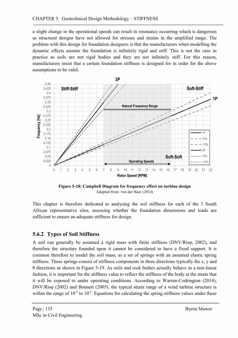
CHAPTER 5: Geotechnical Design Methodology – STIFFNESS
Page | 135 Byron Mawer MSc in Civil Engineering
a slight change in the operational speeds can result in resonance occurring which is dangerous as structural designs have not allowed for stresses and strains in the amplified range. The problem with this design for foundation designers is that the manufacturers when modelling the dynamic effects assume the foundation is infinitely rigid and stiff. This is not the case in practice as soils are not rigid bodies and they are not infinitely stiff. For this reason, manufacturers insist that a certain foundation stiffness is designed for in order for the above assumptions to be valid.
Figure 5-18: Campbell Diagram for frequency effect on turbine design
Adapted from: von der Haar (2014) This chapter is therefore dedicated to analysing the soil stiffness for each of the 3 South African representative sites, assessing whether the foundation dimensions and loads are sufficient to ensure an adequate stiffness for design.
5.6.2 Types of Soil Stiffness A soil can generally be assumed a rigid mass with finite stiffness (DNV/Risφ, 2002), and therefore the structure founded upon it cannot be considered to have a fixed support. It is common therefore to model the soil mass, as a set of springs with an assumed elastic spring stiffness. These springs consist of stiffness components in three directions typically the z, y and θ directions as shown in Figure 5-19. As soils and rock bodies actually behave in a non-linear fashion, it is important for the stiffness value to reflect the stiffness of the body at the strain that it will be exposed to under operating conditions. According to Warren-Codrington (2014), DNV/Risφ (2002) and Bonnett (2005), the typical strain range of a wind turbine structure is within the range of 10-3 to 10-2. Equations for calculating the spring stiffness values under these
0
0.025
0.05
0.075
0.1
0.125
0.15
0.175
0.2
0.225
0.25
0.275
0.3
0.325
0.35
0.375
0.4
0.425
0.45
0 1 2 3 4 5 6 7 8 9 10 11 12 13 14 15 16 17 18 19 20 21 22
Fre
qu
ency
[H
z]
Rotor Speed [RPM]
1P
10%
-10%
3P
10%
-10%
Stiff-Stiff Soft-Stiff
Soft-Soft
3P
1P
Operating Speeds
Natural Frequency Range

CHAPTER 5: Geotechnical Design Methodology – STIFFNESS
Page | 136 Byron Mawer MSc in Civil Engineering
assumptions often relate stiffness to the shear modulus of the soil (G) which can be calculated by applying a stiffness reduction curve to the small strain shear modulus (G0) obtained from the CSW test data in Section 4.3. This is the main reason that these tests are conducted on site, in order to generate the G values needed for foundation stiffness checks.
Figure 5-19: Foundation soil stiffness components
For traditional foundations, designing for seismic and cyclic loads for wind, wave and earthquake action (typically high frequency) makes use of a dynamic shear modulus or elasticity modulus value, which accounts for the repetitive cycles of loading. This value is typically far higher than the static shear and elasticity modulus and is calculated most commonly from the empirical relations developed by Stroud (1989). This generally results in a value of about 3 times larger than the equivalent static value. However, for wind turbine foundations, DNV/Risφ (2002) as well as the manufacturer’s specifications for Vestas and GE, stipulate that vibrations generated by a wind turbine are far more accurately reflected by the static stiffness parameters and therefore the dynamic stiffness parameters are assumed equal to the static values for the purposes of design. In order to calculate the stiffness values in each direction, DNV/Risφ (2002) presents equations based on the soil and embedment conditions of the foundations. This is founded on theory covered in some description by authors such as Bowles (1997) and Das (2011b). For each of the sites being investigated, the applicable sets of equations shown below have been used in order to calculate the soil stiffness in each of the z, y and θ directions [see Table 5-28a), b)] The manufacturers provide limits on the allowable stiffness in the z, y and θ directions (see Table 5-49), although the θ direction or the rocking stiffness as it is commonly known, is the most important for design. This is because rocking vibrations typically dominate the vibrations experienced by foundation (Bu, 2005) which leads to high strains under the footing edge (10-2). The rocking stiffness can also govern the allowable rotation of the structure through the soil
kz
kϴ
ky

CHAPTER 5: Geotechnical Design Methodology – STIFFNESS
Page | 137 Byron Mawer MSc in Civil Engineering
R
H G, v
ROCK
body, which also helps prevent differential settlement from occurring. The equations for the calculation of stiffness are included below:
Table 5-48 a): Equations for the calculation of soil stiffness (DNV/Risφ, 2002)
Stratum over bedrock
Stratum of half-space
Direction Stiffness Equation Stiffness Equation
Kv
𝐾𝑣 =4𝐺𝑅
1 − 𝑣(1 + 1.28
𝑅
𝐻)
𝐾𝑣 =4𝐺𝑅
1 − 𝑣(
1 + 1.28 𝑅𝐻
1 + 1.28𝑅𝐻
𝐺1𝐺2
)
KH
𝐾ℎ =8𝐺𝑅
2 − 𝑣(1 + 0.5
𝑅
𝐻)
𝐾ℎ =8𝐺𝑅
2 − 𝑣(
1 +𝑅
2𝐻
1 +𝑅
2𝐻𝐺1𝐺2
)
Kφ
𝐾∅ =8𝐺𝑅3
3(1 − 𝑣)(1 +
𝑅
6𝐻)
𝐾∅ =8𝐺𝑅3
3(1 − 𝑣)(
1 +𝑅
6𝐻
1 +𝑅
6𝐻𝐺1𝐺2
)
R
H1
G2, v
2
G1, v
1
∞
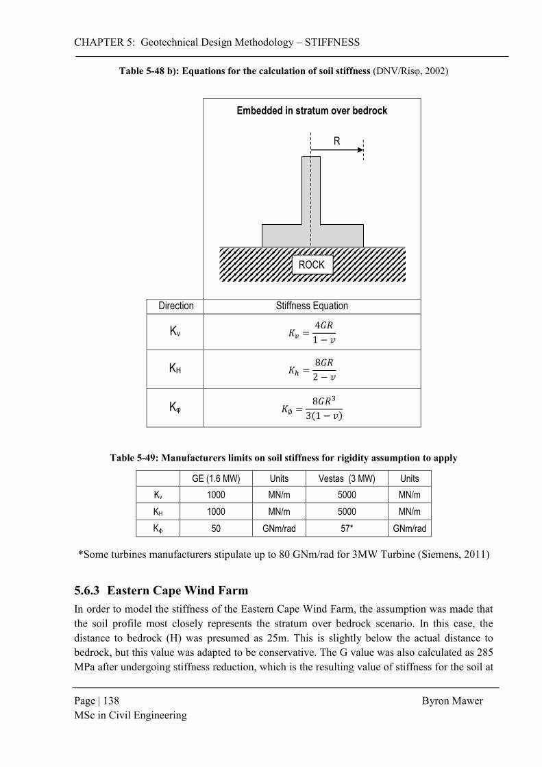
CHAPTER 5: Geotechnical Design Methodology – STIFFNESS
Page | 138 Byron Mawer MSc in Civil Engineering
R
ROCK
Table 5-48 b): Equations for the calculation of soil stiffness (DNV/Risφ, 2002)
Table 5-49: Manufacturers limits on soil stiffness for rigidity assumption to apply
GE (1.6 MW) Units Vestas (3 MW) Units
Kv 1000 MN/m 5000 MN/m
KH 1000 MN/m 5000 MN/m
Kφ 50 GNm/rad 57* GNm/rad
*Some turbines manufacturers stipulate up to 80 GNm/rad for 3MW Turbine (Siemens, 2011)
5.6.3 Eastern Cape Wind Farm In order to model the stiffness of the Eastern Cape Wind Farm, the assumption was made that the soil profile most closely represents the stratum over bedrock scenario. In this case, the distance to bedrock (H) was presumed as 25m. This is slightly below the actual distance to bedrock, but this value was adapted to be conservative. The G value was also calculated as 285 MPa after undergoing stiffness reduction, which is the resulting value of stiffness for the soil at
Embedded in stratum over bedrock
Direction Stiffness Equation
Kv 𝐾𝑣 =4𝐺𝑅
1 − 𝑣
KH 𝐾ℎ =8𝐺𝑅
2 − 𝑣
Kφ 𝐾∅ =8𝐺𝑅3
3(1 − 𝑣)

CHAPTER 5: Geotechnical Design Methodology – STIFFNESS
Page | 139 Byron Mawer MSc in Civil Engineering
the founding level of 3m. The results (as shown in Table 5-50), indicate that a footing of radius 4m or greater would be sufficient to meet the stiffness requirements of both GE and Vestas. In the case of the 21m diameter assumed design, the stiffness can be calculated to be equal to 26 339 MN/m, 17 069 MN/m and 1347 GNm/rad for each of the stiffness directions respectively. These are far above that of the requirements of both design guides and therefore this foundation design satisfies the stiffness design criteria.
Table 5-50: Results of stiffness checks for Eastern Cape Wind Farm
RADIUS (m)
3 4 5 6.25 7.5 9 10.5 12.5
KV (MN/m) 5646 7862 10245 13459 16934 21449 26339 33444
KH (MN/m) 4272 5804 7389 9447 11588 14268 17069 20993
Kφ (MN/m) 29953 71463 140483 276594 481778 840442 1347120 2301264
Kφ (GNm/rad) 30 71 140 277 482 840 1347 2301
5.6.4 Western Cape Wind Farm For the Western Cape Wind Farm, the soil profile most closely represents the stratum over bedrock scenario, similarly to the Eastern Cape Wind Farm. For this design, the distance to bedrock (H) was assumed as 20m based on the soil profile. The G value was calculated to be 63 MPa after undergoing stiffness reduction on a 80 MPa result for G0 from CSW testing for the first 6 -10m of the soil profile. This was not the value for the soil at the founding depth, although it is the weakest soil in the profile, and therefore the value of 63 MPa was chosen to be conservative for the design. The results (as shown in Table 5-51), indicate that a footing of radius between 10-25m would be sufficient to meet the stiffness requirements of both GE and Vestas specifications, with KH being critical in this case. With a 23m diameter footing size, the stiffness can be calculated to be equal to 8090 MN/m, 5334 MN/m and 677 GNm/rad for each of the stiffness directions respectively. These are above that of the requirements of both design guides and therefore this foundation design satisfies the stiffness design criteria.
Table 5-51: Results of stiffness checks for Western Cape Wind Farm
RADIUS (m)
3 4 5 6.25 7.5 9 11 12.5
KV (MN/m) 2140 2787 3485 4430 5458 6800 7978 10398
KH (MN/m) 1725 2094 2477 2977 3501 4160 5091 5829
Kφ (MN/m) 22173 44155 76504 134453 215481 348826 599720 852414
Kφ (GNm/rad) 22 44 77 134 215 349 600 852
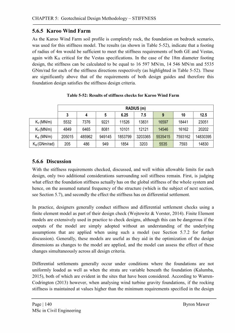
CHAPTER 5: Geotechnical Design Methodology – STIFFNESS
Page | 140 Byron Mawer MSc in Civil Engineering
5.6.5 Karoo Wind Farm As the Karoo Wind Farm soil profile is completely rock, the foundation on bedrock scenario, was used for this stiffness model. The results (as shown in Table 5-52), indicate that a footing of radius of 4m would be sufficient to meet the stiffness requirements of both GE and Vestas, again with KH critical for the Vestas specifications. In the case of the 18m diameter footing design, the stiffness can be calculated to be equal to 16 597 MN/m, 14 546 MN/m and 5535 GNm/rad for each of the stiffness directions respectively (as highlighted in Table 5-52). These are significantly above that of the requirements of both design guides and therefore this foundation design satisfies the stiffness design criteria.
Table 5-52: Results of stiffness checks for Karoo Wind Farm
RADIUS (m)
3 4 5 6.25 7.5 9 10 12.5
KV (MN/m) 5532 7376 9221 11526 13831 16597 18441 23051
KH (MN/m) 4849 6465 8081 10101 12121 14546 16162 20202
Kφ (MN/m) 205015 485962 949145 1853799 3203365 5535415 7593162 14830395
Kφ (GNm/rad) 205 486 949 1854 3203 5535 7593 14830
5.6.6 Discussion With the stiffness requirements checked, discussed, and well within allowable limits for each design, only two additional considerations surrounding soil stiffness remain. First, is judging what effect the foundation stiffness actually has on the global stiffness of the whole system and hence, on the assumed natural frequency of the structure (which is the subject of next section, see Section 5.7), and secondly the effect the stiffness has on differential settlement. In practice, designers generally conduct stiffness and differential settlement checks using a finite element model as part of their design check (Wojtowitz & Vorster, 2014). Finite Element models are extensively used in practice to check designs, although this can be dangerous if the outputs of the model are simply adopted without an understanding of the underlying assumptions that are applied when using such a model (see Section 5.7.2 for further discussion). Generally, these models are useful as they aid in the optimization of the design dimensions as changes to the model are applied, and the model can assess the effect of these changes simultaneously across all design criteria. Differential settlements generally occur under conditions where the foundations are not uniformly loaded as well as when the strata are variable beneath the foundation (Kalumba, 2015), both of which are evident in the sites that have been considered. According to Warren-Codrington (2013) however, when analysing wind turbine gravity foundations, if the rocking stiffness is maintained at values higher than the minimum requirements specified in the design
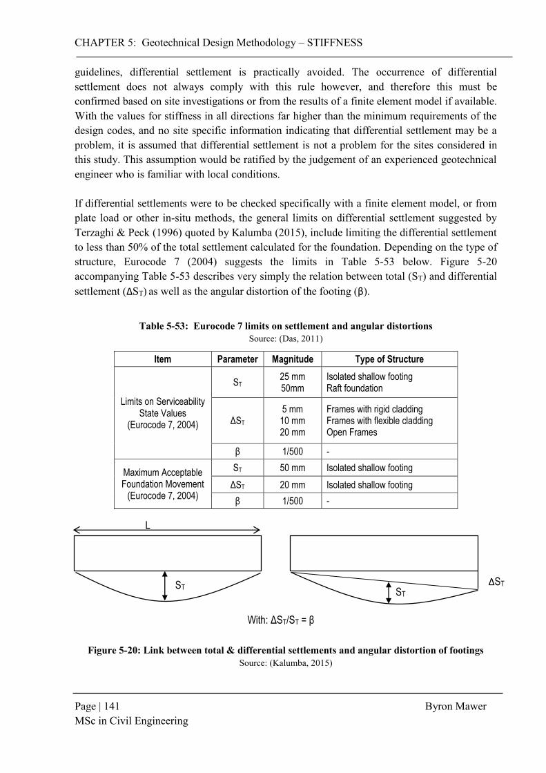
CHAPTER 5: Geotechnical Design Methodology – STIFFNESS
Page | 141 Byron Mawer MSc in Civil Engineering
guidelines, differential settlement is practically avoided. The occurrence of differential settlement does not always comply with this rule however, and therefore this must be confirmed based on site investigations or from the results of a finite element model if available. With the values for stiffness in all directions far higher than the minimum requirements of the design codes, and no site specific information indicating that differential settlement may be a problem, it is assumed that differential settlement is not a problem for the sites considered in this study. This assumption would be ratified by the judgement of an experienced geotechnical engineer who is familiar with local conditions. If differential settlements were to be checked specifically with a finite element model, or from plate load or other in-situ methods, the general limits on differential settlement suggested by Terzaghi & Peck (1996) quoted by Kalumba (2015), include limiting the differential settlement to less than 50% of the total settlement calculated for the foundation. Depending on the type of structure, Eurocode 7 (2004) suggests the limits in Table 5-53 below. Figure 5-20 accompanying Table 5-53 describes very simply the relation between total (ST) and differential settlement (ΔST) as well as the angular distortion of the footing (β).
Table 5-53: Eurocode 7 limits on settlement and angular distortions
Source: (Das, 2011)
Item Parameter Magnitude Type of Structure
Limits on Serviceability State Values
(Eurocode 7, 2004)
ST 25 mm 50mm
Isolated shallow footing Raft foundation
ΔST 5 mm
10 mm 20 mm
Frames with rigid cladding Frames with flexible cladding Open Frames
β 1/500 -
Maximum Acceptable Foundation Movement
(Eurocode 7, 2004)
ST 50 mm Isolated shallow footing
ΔST 20 mm Isolated shallow footing
β 1/500 -
Figure 5-20: Link between total & differential settlements and angular distortion of footings Source: (Kalumba, 2015)
L
ST ST
ΔST
With: ΔST/ST = β

CHAPTER 5: Geotechnical Design Methodology – NATURAL FREQUECNY
Page | 142 Byron Mawer MSc in Civil Engineering
5.7 Natural Frequency Effects 5.7.1 Introduction With the stiffness calculated for each of the investigation sites, the assumptions surrounding the calculation of the natural frequency of the structure can be revisited. The natural frequency of the wind turbine structure, as mentioned in Section 4.9, is calculated based on two main components, the mass and the global stiffness of the structure. As the mass of the structure remains constant, the only factor that can affect the natural frequency is the global stiffness (See Equation 39).
𝑓𝑛 =1
2𝜋√
𝑘
𝑚
Manufacturer’s technical guidelines predict this natural frequency based on the assumption that the foundation acts as a rigid body, has infinite stiffness and responds in an elastic manner. However, as soils in fact behave non-linearly and have a finite stiffness, the effect that this assumption has on the natural frequency of system requires analysis. In order to do this, a dynamic model of the system is required which calculates firstly, the natural frequency of the structure under the infinite stiffness assumption and secondly, the natural frequency of the structure including the effect of foundation stiffness. These values can then be compared to assess whether the soil stiffness effects the natural frequency of the structure. According to DNV/Risφ (2002), the natural frequency typically increases or decreases by between 0-5% accounting for the effect of a finite foundation stiffness, and up to 20% in special cases. As foundation stiffness is site specific, the effect of this assumption was checked for each of the representative South African investigation sites.
5.7.2 Theory A dynamic model of a wind turbine system is required in order to generate approximate natural frequencies of the system. Using dynamic theory, the model can be based on either a distributed or discrete parameter model, each possessing their own inherent advantages. A distributed model assumes the mass in the system is distributed evenly throughout the structure while a discrete (or lumped) parameter model assumes that the mass is concentrated at certain discrete points (see Figure 5-21). The advantages of the lumped parameter model according to Clough & Penzien (2003), is that the model limits the number of degrees of freedom that must be considered when conducting a dynamic analysis, which greatly simplifies the analysis required. It also allows the structure itself to be considered weightless other than at the selected discrete points, which can make the analysis simpler. As a wind turbine system typically has the majority of its mass concentrated at the nacelle and rotor, the lumped parameter model most accurately reflects the distribution of mass through the structure and therefore the dynamic model used is based on this method.

CHAPTER 5: Geotechnical Design Methodology – NATURAL FREQUECNY
Page | 143 Byron Mawer MSc in Civil Engineering
Figure 5-21: Simplified beam lumped parameter system Source: (Clough & Penzien, 2003)
Using a simplified view of a wind turbine system, as shown in Figure 5-22, a dynamic model can be created assuming a lumped mass M, is supported by a weightless cantilevered column with stiffness E, moment of inertia I and length H. This system is then supported by a set of equivalent linear springs, each with their own distinct stiffness based on the strain-dependent stiffness values calculated in Section 5.6. This model can then be used in order to derive the equations required to calculate the natural frequency of the system, from first principles.
Figure 5-22: Simplified wind turbine lumped parameter model Adapted from: (Byrne, 2011)
Both of the models, including one that predicts the natural frequency of the system under the infinite stiffness assumptions and one that does not, require the global stiffness of the system to be calculated. For the infinite stiffness assumption, the stiffness of the system is simply described by the stiffness of the tower, E. For the finite stiffness system however, the effective stiffness of the tower and foundation combined is required to predict the global dynamic response of the system. As the foundation and tower can be viewed as two linear springs connected in series, Equation 40 can be used to calculate the effective stiffness of the springs.
KV
Kϴ KH
M
EI μ
H
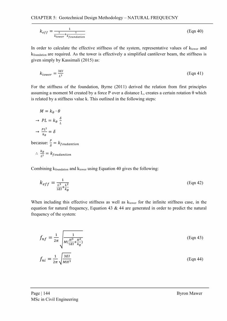
CHAPTER 5: Geotechnical Design Methodology – NATURAL FREQUECNY
Page | 144 Byron Mawer MSc in Civil Engineering
𝑘𝑒𝑓𝑓 =1
1
𝑘𝑡𝑜𝑤𝑒𝑟+
1
𝑘𝑓𝑜𝑢𝑛𝑑𝑎𝑡𝑖𝑜𝑛
(Eqn 40)
In order to calculate the effective stiffness of the system, representative values of ktower and kfoundation are required. As the tower is effectively a simplified cantilever beam, the stiffness is given simply by Kassimali (2015) as:
𝑘𝑡𝑜𝑤𝑒𝑟 =3𝐸𝐼
𝐿3 (Eqn 41) For the stiffness of the foundation, Byrne (2011) derived the relation from first principles assuming a moment M created by a force P over a distance L, creates a certain rotation θ which is related by a stiffness value k. This outlined in the following steps:
𝑀 = 𝑘𝜃 ∙ 𝜃
→ 𝑃𝐿 = 𝑘𝜃 𝛿
𝐿
→ 𝑃𝐿2
𝑘𝜃= 𝛿
becasue: 𝑃
𝛿= 𝑘𝑓𝑜𝑢𝑑𝑎𝑛𝑡𝑖𝑜𝑛
∴ 𝑘𝜃
𝐿2= 𝑘𝑓𝑜𝑢𝑑𝑎𝑛𝑡𝑖𝑜𝑛
Combining kfoundation and ktower using Equation 40 gives the following:
𝑘𝑒𝑓𝑓 =1
𝐿3
3𝐸𝐼+
𝐿2
𝑘𝜃
(Eqn 42)
When including this effective stiffness as well as ktower for the infinite stiffness case, in the equation for natural frequency, Equation 43 & 44 are generated in order to predict the natural frequency of the system:
𝑓𝑛𝑓 =1
2𝜋 √1
𝑀(𝐻3
3𝐸𝐼+
𝐻2
𝑘∅) (Eqn 43)
𝑓𝑛𝑖 =1
2𝜋√
3𝐸𝐼
𝑀𝐻3 (Eqn 44)

CHAPTER 5: Geotechnical Design Methodology – NATURAL FREQUECNY
Page | 145 Byron Mawer MSc in Civil Engineering
As these formulations have been derived from a simplified system, an empirical equation generated by van der Tempel (2002) based on the same principles as the Byrne (2011) method was also used for means of comparison. All assumptions made in both the Byrne and van der Tempel models were equivalent except that van der Tempel allowed for the mass of the tower to be included in calculations. This resulted in the Equation 45 & 46 for both the finite and infinite stiffness cases, where µ is the mass per meter of the tower in kg/m:
𝑓𝑛𝑓 =1
2𝜋 √1
(𝑚+0.227𝜇𝐻)(𝐻3
3𝐸𝐼+
𝐻2
𝑘∅) (Eqn 45)
𝑓𝑛𝑖 =1
2𝜋√
3.04𝐸𝐼
(𝑚+0.227𝜇𝐻)𝐻3 (Eqn 46)
To calculate the natural frequencies using the Byrne (2011) and van der Tempel (2002) method, a number of physical properties of the turbine are required. As some of this information is not readily available (such as the Young’s modulus of the steel used), a number of parameters were assumed in the general range of material properties. Information such as the tower mass (m), nacelle and rotor mass (M), average diameter of tower (D), height of tower (H) and average tower wall thickness (t) were obtained from the manufacturers designs where possible. These properties are summarized in Table 5-54 below:
Table 5-54: Summary of properties and parameters used in natural frequency estimation.
M (kg) m (kg) t (m) D (m) H (m) E (GPa) μ (kg/m) I (m4)
GE 1.6 MW 116000 71000 0.28 2.40 95 200 747.4 1.520
Vestas V112 137000 73500 0.32 3.60 84 200 875.0 5.863
Siemens SWT 133000 78000 0.25 3.50 79.5 200 981.1 4.209
where: 𝐼 ≅
1
8𝜋𝐷3𝑡 (van der Tempel, 2002)
In order to assess whether the structure will vibrate at the natural frequencies and in turn causing resonance, the range of working frequencies require calculation. The working frequencies are based on the rotor rotation frequency (1P) as well as the blade passing frequency (3P) as discussed in Section 5.6. These are calculated from the range of operating speeds that each turbine experiences. These are simply converted from a RPM value to Hz in order to generate the working frequency values. This is summarized for a GE 1.6 MW, Vestas 3 MW and Siemens 3 MW turbine, each with a unique operating speed range (Table 5-55). To illustrate this more effectively, Figure 5-23 & 5-24 show the operating range of working frequencies graphically compared with the stiffness design ranges discussed in Section 5.6.

CHAPTER 5: Geotechnical Design Methodology – NATURAL FREQUECNY
Page | 146 Byron Mawer MSc in Civil Engineering
Table 5-55: Summary of operating speeds and working frequencies for range of turbines
LOW (rpm) HIGH (rpm) 1P LOW 1P HIGH 3P LOW 3P HIGH
GE 1.6 - 82.5 9.75 15.33 0.163 0.255 0.488 0.767
Vestas V112 6.7 17.7 0.112 0.295 0.335 0.885
Siemens SWT 6 16 0.100 0.266 0.300 0.800
Figure 5-23: Working frequency ranges for GE 1.6 MW turbine
Figure 5-24: Working frequency ranges for Vestas 3MW turbine
0 0.1 0.2 0.3 0.4 0.5 0.6 0.7 0.8 0.9 1
FREQUENCY [Hz]
0 0.1 0.2 0.3 0.4 0.5 0.6 0.7 0.8 0.9 1
FREQUENCY [Hz]
SOFT-SOFT SOFT-STIFF STIFF-STIFF
1P
LOW
1P
HIGH
3P
HIGH
3P
LOW
1P
LOW
1P
HIGH
3P
LOW
3P
HIGH
SOFT-STIFF SOFT-SOFT STIFF-STIFF
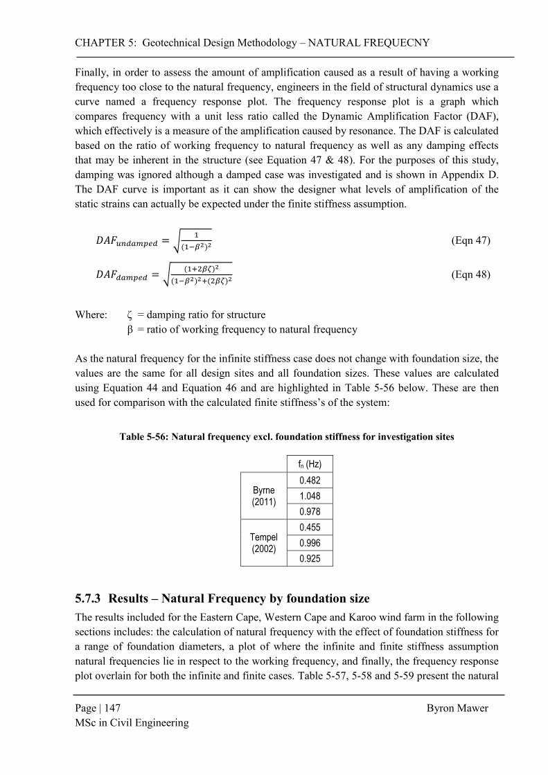
CHAPTER 5: Geotechnical Design Methodology – NATURAL FREQUECNY
Page | 147 Byron Mawer MSc in Civil Engineering
Finally, in order to assess the amount of amplification caused as a result of having a working frequency too close to the natural frequency, engineers in the field of structural dynamics use a curve named a frequency response plot. The frequency response plot is a graph which compares frequency with a unit less ratio called the Dynamic Amplification Factor (DAF), which effectively is a measure of the amplification caused by resonance. The DAF is calculated based on the ratio of working frequency to natural frequency as well as any damping effects that may be inherent in the structure (see Equation 47 & 48). For the purposes of this study, damping was ignored although a damped case was investigated and is shown in Appendix D. The DAF curve is important as it can show the designer what levels of amplification of the static strains can actually be expected under the finite stiffness assumption.
𝐷𝐴𝐹𝑢𝑛𝑑𝑎𝑚𝑝𝑒𝑑 = √1
(1−𝛽2)2 (Eqn 47)
𝐷𝐴𝐹𝑑𝑎𝑚𝑝𝑒𝑑 = √(1+2𝛽 )2
(1−𝛽2)2+(2𝛽 )2 (Eqn 48)
Where: ζ = damping ratio for structure
β = ratio of working frequency to natural frequency As the natural frequency for the infinite stiffness case does not change with foundation size, the values are the same for all design sites and all foundation sizes. These values are calculated using Equation 44 and Equation 46 and are highlighted in Table 5-56 below. These are then used for comparison with the calculated finite stiffness’s of the system:
Table 5-56: Natural frequency excl. foundation stiffness for investigation sites
fn (Hz)
Byrne (2011)
0.482
1.048
0.978
Tempel (2002)
0.455
0.996
0.925
5.7.3 Results – Natural Frequency by foundation size The results included for the Eastern Cape, Western Cape and Karoo wind farm in the following sections includes: the calculation of natural frequency with the effect of foundation stiffness for a range of foundation diameters, a plot of where the infinite and finite stiffness assumption natural frequencies lie in respect to the working frequency, and finally, the frequency response plot overlain for both the infinite and finite cases. Table 5-57, 5-58 and 5-59 present the natural

CHAPTER 5: Geotechnical Design Methodology – NATURAL FREQUECNY
Page | 148 Byron Mawer MSc in Civil Engineering
frequency response for each site investigated by foundation size while Figure 5-25, 5-26 and 5-27 shows the effect the finite stiffness assumption has on the natural frequency for each design.
Table 5-57: Natural frequency incl. foundation stiffness for Eastern Cape Wind Farm
RADIUS OF FOOTING
3 4 5 6.25 7.5 9 10 12.5
fn (Hz) fn (Hz) fn (Hz) fn (Hz) fn (Hz) fn (Hz) fn (Hz) fn (Hz)
Byrne (2011)
GE 1.6 MW 0.431 0.458 0.470 0.476 0.478 0.480 0.480 0.481
Vestas 3MW 0.722 0.866 0.943 0.990 1.014 1.028 1.033 1.040
Siemens 3MW 0.722 0.842 0.902 0.937 0.954 0.964 0.968 0.973
Tempel (2002)
GE 1.6 MW 0.403 0.429 0.440 0.446 0.448 0.450 0.450 0.451
Vestas 3MW 0.683 0.820 0.892 0.937 0.959 0.972 0.977 0.984
Siemens 3MW 0.682 0.795 0.851 0.885 0.901 0.911 0.914 0.919
Table 5-58: Natural frequency incl. foundation stiffness for Western Cape Wind Farm
RADIUS OF FOOTING
3 4 5 6.25 7.5 9 10 12.5
fn (Hz) fn (Hz) fn (Hz) fn (Hz) fn (Hz) fn (Hz) fn (Hz) fn (Hz)
Byrne (2011)
GE 1.6 MW 0.195 0.332 0.403 0.437 0.454 0.466 0.472 0.475
Vestas V112 0.217 0.434 0.616 0.750 0.842 0.915 0.959 0.990
Siemens 0.232 0.453 0.627 0.746 0.822 0.880 0.913 0.937
Tempel (2002)
GE 1.6 MW 0.183 0.311 0.377 0.409 0.426 0.436 0.442 0.446
Vestas V112 0.206 0.411 0.583 0.710 0.797 0.865 0.907 0.936
Siemens 0.219 0.428 0.592 0.705 0.777 0.831 0.863 0.885
Table 5-59: Natural frequency incl. foundation stiffness for Karoo Wind Farm
RADIUS OF FOOTING
3 4 5 6.25 7.5 9 10 12.5
fn (Hz) fn (Hz) fn (Hz) fn (Hz) fn (Hz) fn (Hz) fn (Hz) fn (Hz)
Byrne (2011)
GE 1.6 MW 0.460 0.472 0.477 0.479 0.480 0.481 0.481 0.482
Vestas V112 0.879 0.965 1.003 1.024 1.034 1.039 1.042 1.045
Siemens 0.852 0.919 0.946 0.962 0.969 0.973 0.974 0.976
Tempel (2002)
GE 1.6 MW 0.431 0.443 0.447 0.449 0.450 0.451 0.451 0.451
Vestas V112 0.831 0.913 0.949 0.969 0.978 0.983 0.985 0.988
Siemens 0.805 0.867 0.894 0.908 0.915 0.919 0.920 0.922
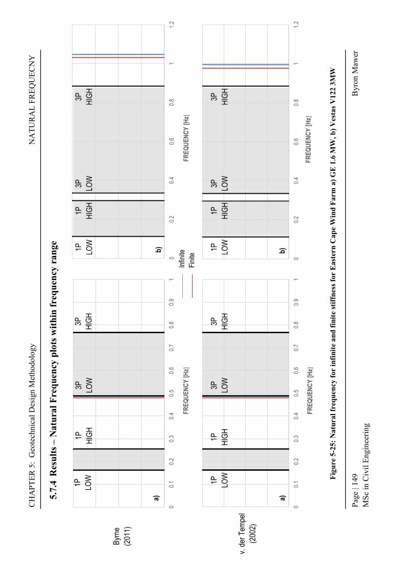
CH
APT
ER 5
: G
eote
chni
cal D
esig
n M
etho
dolo
gy
N
ATU
RA
L FR
EQU
ECN
Y
Page
| 14
9
B
yron
Maw
er
MSc
in C
ivil
Engi
neer
ing
00.
10.
20.
30.
40.
50.
60.
70.
80.
91
FR
EQ
UE
NC
Y [
Hz]
00.
10.
20.
30.
40.
50.
60.
70.
80.
91
FR
EQ
UE
NC
Y [
Hz]
00.
20.
40.
60.
81
1.2
FR
EQ
UE
NC
Y [
Hz]
5.7.
4 R
esul
ts –
Nat
ural
Fre
quen
cy p
lots
with
in fr
eque
ncy
rang
e
Figu
re 5
-25:
Nat
ural
freq
uenc
y fo
r in
finite
and
fini
te st
iffne
ss fo
r E
aste
rn C
ape
Win
d Fa
rm a
) GE
1.6
MW
, b) V
esta
s V12
2 3M
W
00.
20.
40.
60.
81
1.2
FR
EQ
UE
NC
Y [
Hz]
1P
LOW
1P
HIG
H
3P
LOW
3P
HIG
H
1P
LOW
1P
HIG
H
3P
LOW
3P
HIG
H
1P
LOW
1P
HIG
H
3P
LOW
3P
HIG
H
1P
LOW
1P
HIG
H
3P
LOW
3P
HIG
H
Infin
ite
Fin
ite
Byr
ne
(201
1)
v. d
er T
empe
l
(200
2)
b)
a)
a)
b)

CH
APT
ER 5
: G
eote
chni
cal D
esig
n M
etho
dolo
gy
N
ATU
RA
L FR
EQU
ECN
Y
Page
| 15
0
B
yron
Maw
er
MSc
in C
ivil
Engi
neer
ing
00.
10.
20.
30.
40.
50.
60.
70.
80.
91
FR
EQ
UE
NC
Y [
Hz]
00.
20.
40.
60.
81
1.2
FR
EQ
UE
NC
Y [
Hz]
00.
10.
20.
30.
40.
50.
60.
70.
80.
91
FR
EQ
UE
NC
Y [
Hz]
00.
20.
40.
60.
81
1.2
FR
EQ
UE
NC
Y [
Hz]
Figu
re 5
-26:
Nat
ural
freq
uenc
y fo
r in
finite
and
fini
te st
iffne
ss fo
r W
este
rn C
ape
Win
d Fa
rm a
) GE
1.6
MW
, b) V
esta
s V12
2 3M
W
Infin
ite
Fin
ite
1P
LOW
1P
HIG
H
3P
LOW
3P
HIG
H
1P
LOW
1P
HIG
H
3P
LOW
3P
HIG
H
1P
LOW
1P
HIG
H
3P
LOW
3P
HIG
H
1P
LOW
1P
HIG
H
3P
LOW
3P
HIG
H
Byr
ne
(201
1)
v. d
er T
empe
l
(200
2)
a)
a)
b)
b)

CH
APT
ER 5
: G
eote
chni
cal D
esig
n M
etho
dolo
gy
N
ATU
RA
L FR
EQU
ECN
Y
Page
| 15
1
B
yron
Maw
er
MSc
in C
ivil
Engi
neer
ing
Fi
gure
5-2
7: N
atur
al fr
eque
ncy
for
infin
ite a
nd fi
nite
stiff
ness
for
Kar
oo W
ind
Farm
a) G
E 1
.6 M
W, b
) Ves
tas V
122
3MW
00.
10.
20.
30.
40.
50.
60.
70.
80.
91
FR
EQ
UE
NC
Y [
Hz]
00.
20.
40.
60.
81
1.2
FR
EQ
UE
NC
Y [
Hz]
00.
10.
20.
30.
40.
50.
60.
70.
80.
91
FR
EQ
UE
NC
Y [
Hz]
00.
20.
40.
60.
81
1.2
FR
EQ
UE
NC
Y [
Hz]
1P
LOW
1P
HIG
H
3P
LOW
3P
HIG
H
1P
LOW
1P
HIG
H
3P
LOW
3P
HIG
H
1P
LOW
1P
HIG
H
3P
LOW
3P
HIG
H
1P
LOW
1P
HIG
H
3P
LOW
3P
HIG
H
Infin
ite
Fin
ite
Byr
ne
(201
1)
v. d
er T
empe
l
(200
2)
b) b)
a) a)

CHAPTER 5: Geotechnical Design Methodology - NATURAL FREQUECNY
Page | 152 Byron Mawer MSc in Civil Engineering
0.0
2.0
4.0
6.0
8.0
10.0
12.0
0 0.2 0.4 0.6 0.8 1 1.2 1.4 1.6 1.8 2 2.2
DA
F
β
GE Incl.Stiffness
Vestas Incl.Stiffness
GE Excl.Stiffness
Vestas Excl.Stiffness
0.0
2.0
4.0
6.0
8.0
10.0
12.0
0 0.2 0.4 0.6 0.8 1 1.2 1.4 1.6 1.8 2 2.2
DA
F
β
GE Incl.Stiffness
Vestas Incl.Stiffness
GE Excl.Stiffness
Vestas Excl.Stiffness
0.0
2.0
4.0
6.0
8.0
10.0
12.0
0 0.2 0.4 0.6 0.8 1 1.2 1.4 1.6 1.8 2 2.2
DA
F
β
GE Incl.Stiffness
Vestas Incl.Stiffness
GE Excl.Stiffness
Vestas Excl.Stiffness
5.7.5 Results – Dynamic amplification effects
Figure 5-28: Effect on Dynamic Amplification for Eastern Cape Wind Farm (R=10)
Figure 5-29: Effect on Dynamic Amplification for Western Cape Wind Farm (R=10)
Figure 5-30: Effect on Dynamic Amplification for Karoo Wind Farm (R=9)
CHAPTER 5: Geotechnical Design Methodology - NATURAL FREQUECNY
Page | 153 Byron Mawer MSc in Civil Engineering
5.7.6 Discussion & Summary From the results presented, a number of trends and relationships can be found between the foundation stiffness and the effect on natural frequency. Using the tables presented in Section 5.7.5, it can be seen that natural frequency, using the finite stiffness assumption, gets closer to value predicted with the infinite stiffness assumption as the foundation size increases. This is expected as the soil stiffness will increase with foundation size (as shown in Section 5.6) and hence, the stiffness will begin to tend to a value large enough to have very little effect on the natural frequency. At foundation diameters of 20m+, the percentage difference in natural frequency between the finite and infinite stiffness assumption is generally less than 2%, which is negligible for design purposes. This is also in-line with DNV/Risφ (2002) predictions. As the turbine foundation size is generally limited to at least 16m in diameter to avoid gapping, for stiff South African soils, the infinite stiffness assumption could effectively be used with little concern for its effect on design. For less stiff soils, this is not true. When consulting the graphs of natural frequency against working frequency in Section 5.7.5, it is evident that the GE turbine has been designed in the soft-stiff range while the Vestas turbine for the Stiff-Stiff range. The reason for the Vestas turbine being designed in the stiff-stiff range is due to the narrow range of safe frequencies available for designing in the soft-stiff range. Any error in the assumption of natural frequency would have resulted in resonance occurring at some 1P High or 3P Low working frequency value of the turbine. These graphs also clearly indicate the notable difference in natural frequency caused by including the foundation stiffness for less stiff soils in calculation. When comparing the Eastern Cape and Karoo wind farm, which have a relatively high inherent stiffness profile, with that of the Western Cape Wind Farm, with an inherently low stiffness profile, it can be seen that the difference in natural frequency is far more pronounced for that of the Western Cape farm. If the Vestas 3MW tower had been designed for a lower natural frequency in order to be more cost-effective, they would have found after checking for the effect of foundation stiffness, that their turbine would have a natural frequency within the 3P working frequency range at which point resonance would occur. This emphasizes how important it is to check the natural frequency assumption for design for soils with weaker stiffness profiles and provides evidence for why it should be included in all site-specific design checks. For the structural engineers, the change in design for the dynamic amplification caused at certain operating frequencies is evident from the graphs in Figure 5-28, 5-29 & 5-30. For example, consider the change of natural frequency due to foundation stiffness for the Western Cape Wind farm: at a β value of 0.9, a strain amplification of 3.8 was expected using the infinite stiffness assumption. Because of the reduced natural frequency, at a β value of 0.9, the DAF becomes 7.44, significantly higher than what was designed for. For higher stiffness values, such as in Figure 5-29 & 5-30, this effect is less pronounced. For this reason, it should be ensured in design either that the foundation stiffness is accounted for in the natural frequency prediction or that the foundation is designed to be significantly big that the infinite stiffness assumption is valid. It is also a validation that the Byrne (2011) and van der Tempel

CHAPTER 5: Geotechnical Design Methodology - NATURAL FREQUECNY
Page | 154 Byron Mawer MSc in Civil Engineering
(2002) prediction methods are very similar for all foundation sizes and sites, providing a solid foundation for the accuracy of the Byrne method’s prediction value. Table 5-60, 5-61, 5-62 shown below emphasize the difference in natural frequency between the infinite and finite stiffness assumptions by footing size for each investigation site. As the turbines are generally limited by gapping, only foundations with diameter 15m+ have been highlighted. As discussed above, the Eastern Cape and Karoo wind farms both had very stiff profiles and therefore all differences between finite and infinite stiffness assumptions fell within the expected DNV/Risφ (2002) range of 0-5% reduction. For the Western Cape wind farm however, the soil stiffness was significantly lower and hence fell outside the normal range (highlighted orange and red). To conclude, the results of this analysis have highlighted the importance of including foundation stiffness considerations in natural frequency calculations. It is highly recommended therefore that these checks be carried out, at least at a basic level, using this method or using more complicated models with FEM or dynamic design software.
Table 5-60: % Difference in Natural Frequency due to increasing foundation size (EC)
RADIUS OF FOOTING
3 4 5 6.25 7.5 9 10 12.5
% Diff % Diff % Diff % Diff % Diff % Diff % Diff % Diff
Byrne (2011)
GE 1.6 MW 4.7 2.0 1.0 0.5 0.3 0.2 0.1 0.1
Vestas V112 19.2 8.5 4.4 2.3 1.3 0.8 0.6 0.3
Siemens 14.8 6.5 3.4 1.7 1.0 0.6 0.4 0.2
Tempel (2002)
GE 1.6 MW 5.4 2.7 1.7 1.2 1.0 0.8 0.8 0.7
Vestas V112 19.8 9.0 4.9 2.8 1.8 1.3 1.0 0.8
Siemens 15.0 6.7 3.5 1.9 1.1 0.7 0.6 0.4
Table 5-61: % Difference in Natural Frequency due to increasing foundation size (Karoo)
RADIUS OF FOOTING
3 4 5 6.25 7.5 9 10 12.5
% Diff % Diff % Diff % Diff % Diff % Diff % Diff % Diff
Byrne (2011)
GE 1.6 MW 11.9 5.2 2.7 1.4 0.8 0.4 0.3 0.2
Vestas V112 45.0 20.9 11.1 5.8 3.4 1.9 1.4 0.7
Siemens 35.5 16.2 8.5 4.4 2.6 1.5 1.1 0.5
Tempel (2002)
GE 1.6 MW 12.7 5.9 3.3 2.0 1.4 1.1 1.0 0.8
Vestas V112 45.7 21.5 11.6 6.3 3.8 2.4 1.9 1.2
Siemens 35.7 16.4 8.7 4.6 2.7 1.6 1.2 0.7
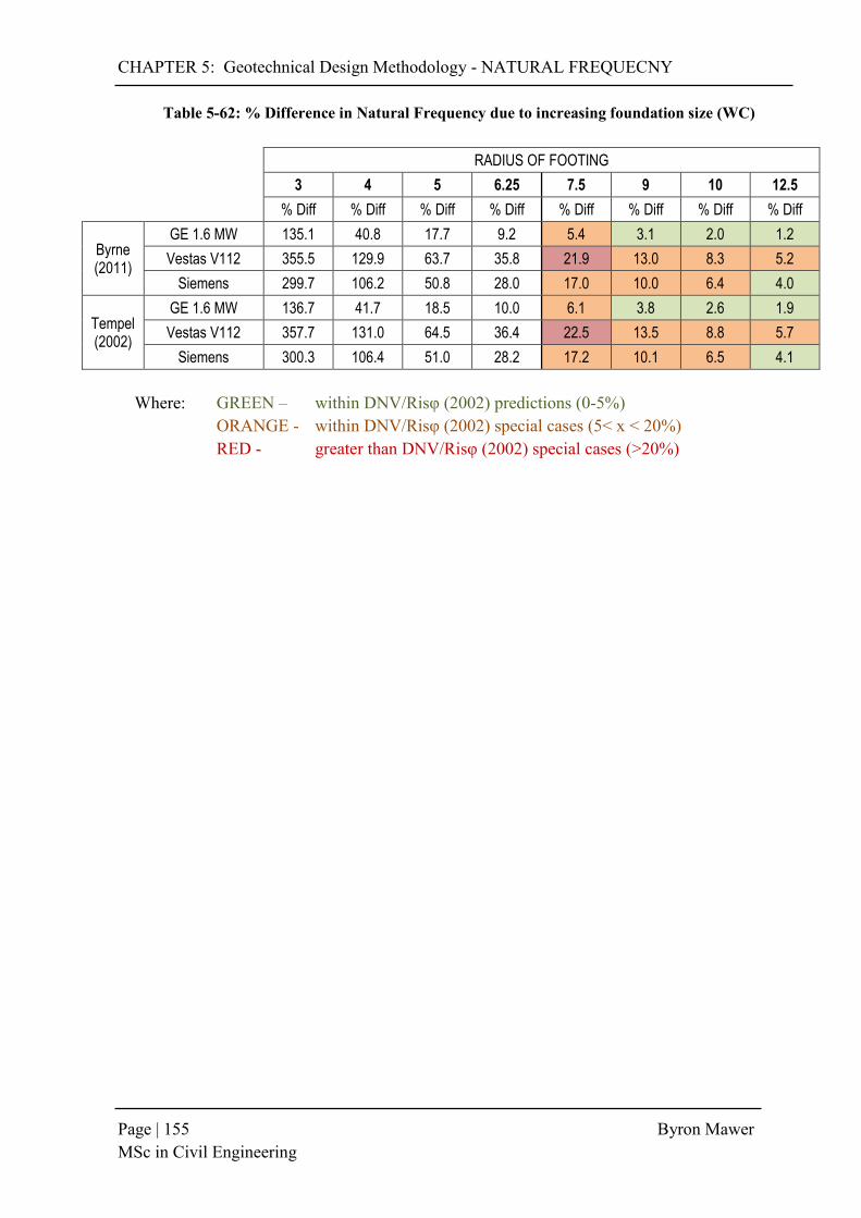
CHAPTER 5: Geotechnical Design Methodology - NATURAL FREQUECNY
Page | 155 Byron Mawer MSc in Civil Engineering
Table 5-62: % Difference in Natural Frequency due to increasing foundation size (WC)
RADIUS OF FOOTING
3 4 5 6.25 7.5 9 10 12.5
% Diff % Diff % Diff % Diff % Diff % Diff % Diff % Diff
Byrne (2011)
GE 1.6 MW 135.1 40.8 17.7 9.2 5.4 3.1 2.0 1.2
Vestas V112 355.5 129.9 63.7 35.8 21.9 13.0 8.3 5.2
Siemens 299.7 106.2 50.8 28.0 17.0 10.0 6.4 4.0
Tempel (2002)
GE 1.6 MW 136.7 41.7 18.5 10.0 6.1 3.8 2.6 1.9
Vestas V112 357.7 131.0 64.5 36.4 22.5 13.5 8.8 5.7
Siemens 300.3 106.4 51.0 28.2 17.2 10.1 6.5 4.1
Where: GREEN – within DNV/Risφ (2002) predictions (0-5%) ORANGE - within DNV/Risφ (2002) special cases (5< x < 20%) RED - greater than DNV/Risφ (2002) special cases (>20%)

CHAPTER 5: Geotechnical Design Methodology – OTHER
Page | 156 Byron Mawer MSc in Civil Engineering
5.8 Other Considerations All geotechnical projects are site-specific and therefore all sites inherently have very particular issues that are not always relevant or expected in a typical design process. As South Africa has a very diverse geological background, there are a number of indigenous soils found in the local wind development corridors possessing troublesome properties that can significantly affect foundation designs. For this reason, as well as to account for wind turbine specific loading and structural issues, this section aims to briefly discuss a number of important issues that should be considered by the engineer. These concerns do not always apply to every project but can have a significant effect on either the expected results or approach to the foundation planning. These considerations include founding on Pedogenic soils, the use of finite element modelling, and issues with foundation gapping.
5.8.1 Foundations on Pedogenic Soils Pedogenic soils are defined by Brink (1979) as soils, which have become cemented or replaced by certain authegenic minerals, often through the breakdown of natural inclusions in the soil profile, resulting in precipitation of minerals into the soil over time. These minerals then have a cementing effect on the surrounding soil particles forming soils with various degrees of hardness. Some common precipitated minerals encountered in South African pedocretes or duricrusts include those of: - calcite (calcrete), - dolomite (dolocrete), - iron oxides (ferricrete), and - silica (silcrete). Netterberg (1994) advises that by definition of the Specialty Session (1976), a soil body containing these minerals be only defined as a pedocrete when soils contain more than 50% of the cementing or replacing material. Further to this, soils with less than a 50% make up of cementing material is described as lateritic, calcified, or ferruginised depending on the mineral make-up of the material. In terms of founding on calcrete material, one has to understand the various types of calcrete that will be encountered and what the resulting founding implications are. Pedocretes can occur in a number of phases or consistencies depending on the type of conditions that were prevalent during their formation. Netterberg (1994) classifies them into 3 distinct groups: - Indurated (hardpans and nodules), - Non-indurated (soft or powder forms), and - Combinations of the two (nodular).

CHAPTER 5: Geotechnical Design Methodology – OTHER
Page | 157 Byron Mawer MSc in Civil Engineering
The problem with hardpan calcrete is that it forms irregularly in the ground and although hardpan calcrete inclusion can act as a soil support similar to that of a buried raft foundation, it is often safer to assume that the calcrete reinforcing effect does not contribute to the stability of the system. This is because it is often very difficult to predict the thickness and extent of the formation in its entirety, and therefore it is dangerous to assume this in design. In the case, where the calcrete can safely be assumed to contribute, the calcrete thickness and strength are important for bearing capacity purposes. This is the reason that the site-specific bearing capacity check of a soil underlain by rigid base at shallow depth is included for the Eastern Cape wind farm, which takes into account this rafting effect by the hardpan calcrete layers found in the profile. Powdered and soft calcrete rarely has issues with expansion but there are notable mentions by Netterbeg (1994) of collapse potential especially if the hardpan calcrete is a weaker than its stronger variations (Beales, 2015). In some instances, the calcrete forms in between sandy transported layers, with loose sandy layers occurring within the hardpan lenses. The result is that the sand layers settle and voids form directly beneath the calcrete, which can lead to collapse under certain structural loadings. This can result in a soil that seems to have a favourable bearing capacity based on the shear strength parameters from field and laboratory testing, while actually experiencing failure under far lower loads. In terms of assessing soil profiles with pedocrete inclusions, it is down to the geotechnical engineer on the project to assess the situation carefully and on the in-situ conditions. Figure 5-31 below, shows the distribution of pedocrete formations across South Africa.
Figure 5-31: Distribution of pedocrete soils in South Africa.
Source: (Netterberg, 1994)

CHAPTER 5: Geotechnical Design Methodology – OTHER
Page | 158 Byron Mawer MSc in Civil Engineering
5.8.2 Finite Element Modelling in Design One of the most common preconceived notions in South Africa surrounding wind turbine foundation planning is the need for use of the finite element method in order to safely prepare a geotechnical and structural design for gravity foundations. As with any engineering software, the predictions that are produced by finite element models are only useful to the designer if the user is able to interpret the results while understanding the assumptions and limitations the program has used. The major advantage of the FEM for wind turbine gravity foundations is that, if setup correctly, they can produce very good estimations of the global rotational stiffness of the soil body (kφ). They can additionally be very effectively used in order to optimize the dimensions of the footings based on all the design conditions, specifically the minimum lateral and rocking stiffness combination, which can often control the size of the footings. For example, for gravity foundations of the West Coast 1 Wind Farm in the Western Cape, Wojtowitz & Vorster (2014) describe the use of a Plaxis 3D FE model in order to determine the optimum combination of factors to meet the design criteria, while ensuring the requirements for stiffness was maintained. The model contained 17,160 No. 15-noded elements with 45,913 No. nodes representing a 90 x 90 x 200m soil block profile (see Figure 5-32). Additionally, a Plaxis 2D version of the same system was also created in order to assess the possibility of softening of the high plasticity material discovered at founding depth, as well as local failure of the contact layer between the foundation and the soil bed. In this case, Plaxis 3D is a useful tool that links the all criteria and footing dimensions in one location allowing for optimization of all the factors at the same time. However, this model is still based completely on the theory and calculations presented in this methodology and therefore the finite element method would not be necessary in order to complete the design. It effectively streamlines and aids the optimization of the process but is based on the same principles and criteria investigated. The Plaxis 2D version of the footing on the other hand, assess site specific problems that are very difficult to assess individually, and as a result has allowed the optimization of the foundation size to be far lower than expected for a soil falling in the Western Cape region. The disadvantages of using the FEM is that a very in depth understanding of the finite element method is required in order to understand which theories, boundary conditions, and constitutive relations best represent the situation of a particular site. For example, in some instances, according to Potts & Zdravkovic (2001), Mohr-Coulomb theory does not always yield representative results for undrained and partially drained conditions and therefore a more appropriate soil stress-strain idealisation may be required. They further add that for the purposes of a FE setup, soil property idealizations are required that best represent the soil behaviour being investigated. In other words, the model that best represents stress and strain relations in a soil mass should be used for bearing capacity design, and the model that best represents deformation in soils should be used for assessing settlement criteria. At the end of
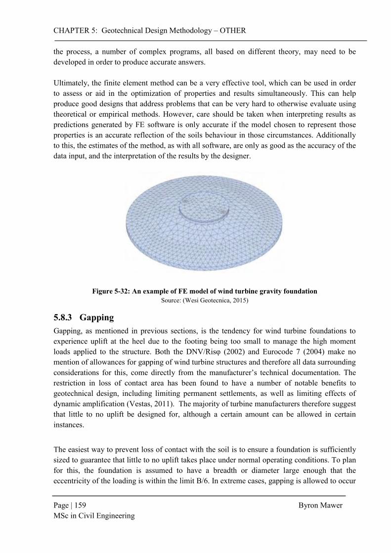
CHAPTER 5: Geotechnical Design Methodology – OTHER
Page | 159 Byron Mawer MSc in Civil Engineering
the process, a number of complex programs, all based on different theory, may need to be developed in order to produce accurate answers. Ultimately, the finite element method can be a very effective tool, which can be used in order to assess or aid in the optimization of properties and results simultaneously. This can help produce good designs that address problems that can be very hard to otherwise evaluate using theoretical or empirical methods. However, care should be taken when interpreting results as predictions generated by FE software is only accurate if the model chosen to represent those properties is an accurate reflection of the soils behaviour in those circumstances. Additionally to this, the estimates of the method, as with all software, are only as good as the accuracy of the data input, and the interpretation of the results by the designer.
Figure 5-32: An example of FE model of wind turbine gravity foundation Source: (Wesi Geotecnica, 2015)
5.8.3 Gapping Gapping, as mentioned in previous sections, is the tendency for wind turbine foundations to experience uplift at the heel due to the footing being too small to manage the high moment loads applied to the structure. Both the DNV/Risφ (2002) and Eurocode 7 (2004) make no mention of allowances for gapping of wind turbine structures and therefore all data surrounding considerations for this, come directly from the manufacturer’s technical documentation. The restriction in loss of contact area has been found to have a number of notable benefits to geotechnical design, including limiting permanent settlements, as well as limiting effects of dynamic amplification (Vestas, 2011). The majority of turbine manufacturers therefore suggest that little to no uplift be designed for, although a certain amount can be allowed in certain instances.
The easiest way to prevent loss of contact with the soil is to ensure a foundation is sufficiently sized to guarantee that little to no uplift takes place under normal operating conditions. To plan for this, the foundation is assumed to have a breadth or diameter large enough that the eccentricity of the loading is within the limit B/6. In extreme cases, gapping is allowed to occur

CHAPTER 5: Geotechnical Design Methodology – OTHER
Page | 160 Byron Mawer MSc in Civil Engineering
SOIL
Mres
+
-
PRESSUE DISTRIBTUION
50% GAPPING
Loss of Contact
within certain limits defined by the manufacturer. Vestas (2011) recommends that if allowed for, only uplift of 25% of the footing base is acceptable to ensure foundation stability. When calculating the percentage gapping, the extreme normal load case (LC 2 in this study) should be considered, acting along the main axis of the foundation and assuming an elastic soil pressure distribution (see Figure 5-33). General Electric (2011b) recommends that the design should comply with the Germanischer Lloyd Wind Energy GmbH IV Rules and Guidelines Edition 2003, 6.7.6.3 Part (3) and Part (4). From this code, 100% contact area between the foundation and soil during normal operational loading is required, and for the extreme load case, at least 50% contact is must be maintained. The problem with allowing for gapping in design is that it directly effects the stiffness of the soil that can be mobilized in rocking. Therefore, the kθ value must be recalculated for a new rotation angle that has been factored to account for the loss of contact area. Equation 49 below, adapted from Vestas (2011) can be used, where CM is spring stiffness of soil in rotation: 𝑘𝜃 =
𝑀
𝜑=
𝑀(𝜎𝑚𝑎𝑥−𝜎𝑚𝑖𝑛)
𝐵𝑒𝑓𝑓∙𝐶𝑀
(Eqn 49)
To avoid this process, it is therefore important to attempt to prevent gapping, although it can be tolerated in design depending on its effects on settlement, foundation stiffness and dynamic amplification. It is vital that the turbine manufacture’s technical guidelines are consulted to assess how their specific turbines should be treated for the allowance of uplift or whether it should be avoided under all loading conditions.
Figure 5-33: Depiction of the maximum allowed gapping for GE turbines

CONCLUSION
Page | 161 Byron Mawer MSc in Civil Engineering
6. CONCLUSION The objective of this study was to create a general geotechnical design methodology addressing wind turbine gravity foundations for South African soil conditions. In developing the methodology, the following concerns were addressed:
1. The scale of the wind energy economy in SA, including the current project uptake and bidding processes that govern the REIPPP programme. Additionally addressed are the future plans for expansion of the industry based on the local Integrated Energy Plan,
2. Turbine types, mechanisms, loading effects and foundation alternatives, with focus on the reasons for gravity foundations being favoured in South Africa, and therefore the justification for their choice as the subject of this research,
3. Key principles, criteria and investigation techniques, that require consideration when planning a wind turbine gravity footing, including reference to current codes of practice, design methodologies and the way in which they can be adapted for local conditions, and
4. Regional case studies, including 3 unique sites with varying soil conditions in each of the 3 major wind development corridors of South Africa, with the aim of adapting this into a general design methodology for local conditions.
6.1 Summary of Design Criteria Results From the work presented in this study, the following criteria were found to be critical, and are listed containing the relevant methods of investigation, the results that have been obtained for the three SA representative case studies, and finally items that have been found to be important considerations during the planning process:
- SITE INVESTIGATIONS: Wind turbine foundation site investigations consist of common laboratory and field-testing methods including SPT, DPSH and lab classification tests, all of which are readily available in SA. Methods unique to wind energy projects include in-situ seismic tests, such as the CSW test, in order to assess the in-situ ground stiffness needed for the foundation stiffness checks. Generally, soil data is needed for depths of 1 – 2 times the breadth of the footing, which is often between 20-30m in depth. An introduction to obtaining Mohr-Coulomb parameters using the Hoek-Brown criteria was also presented for sites dominated by sub-surface rock such as in the Karoo region of the country.
- BEARING CAPACITY: Dimensioning and bearing capacity checks for wind turbine gravity structures are mostly based on the suggestions of the DNV/Risφ (2002) guidelines. This method was presented and the results compared with a number of site-specific bearing capacity analyses as well as empirical DPSH predictions for both a square a circular footing shape. The DPSH empirical results were found to be critical in all cases however they were generally very close to that of
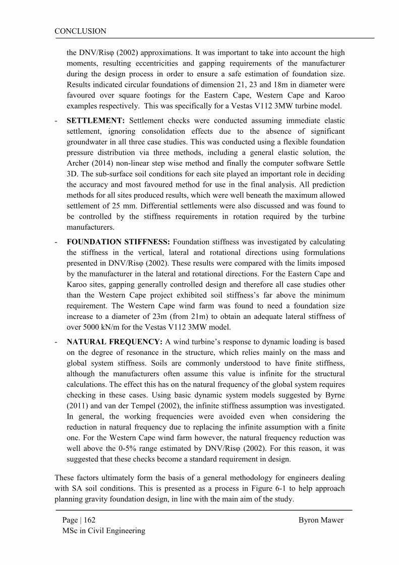
CONCLUSION
Page | 162 Byron Mawer MSc in Civil Engineering
the DNV/Risφ (2002) approximations. It was important to take into account the high moments, resulting eccentricities and gapping requirements of the manufacturer during the design process in order to ensure a safe estimation of foundation size. Results indicated circular foundations of dimension 21, 23 and 18m in diameter were favoured over square footings for the Eastern Cape, Western Cape and Karoo examples respectively. This was specifically for a Vestas V112 3MW turbine model.
- SETTLEMENT: Settlement checks were conducted assuming immediate elastic settlement, ignoring consolidation effects due to the absence of significant groundwater in all three case studies. This was conducted using a flexible foundation pressure distribution via three methods, including a general elastic solution, the Archer (2014) non-linear step wise method and finally the computer software Settle 3D. The sub-surface soil conditions for each site played an important role in deciding the accuracy and most favoured method for use in the final analysis. All prediction methods for all sites produced results, which were well beneath the maximum allowed settlement of 25 mm. Differential settlements were also discussed and was found to be controlled by the stiffness requirements in rotation required by the turbine manufacturers.
- FOUNDATION STIFFNESS: Foundation stiffness was investigated by calculating the stiffness in the vertical, lateral and rotational directions using formulations presented in DNV/Risφ (2002). These results were compared with the limits imposed by the manufacturer in the lateral and rotational directions. For the Eastern Cape and Karoo sites, gapping generally controlled design and therefore all case studies other than the Western Cape project exhibited soil stiffness’s far above the minimum requirement. The Western Cape wind farm was found to need a foundation size increase to a diameter of 23m (from 21m) to obtain an adequate lateral stiffness of over 5000 kN/m for the Vestas V112 3MW model.
- NATURAL FREQUENCY: A wind turbine’s response to dynamic loading is based on the degree of resonance in the structure, which relies mainly on the mass and global system stiffness. Soils are commonly understood to have finite stiffness, although the manufacturers often assume this value is infinite for the structural calculations. The effect this has on the natural frequency of the global system requires checking in these cases. Using basic dynamic system models suggested by Byrne (2011) and van der Tempel (2002), the infinite stiffness assumption was investigated. In general, the working frequencies were avoided even when considering the reduction in natural frequency due to replacing the infinite assumption with a finite one. For the Western Cape wind farm however, the natural frequency reduction was well above the 0-5% range estimated by DNV/Risφ (2002). For this reason, it was suggested that these checks become a standard requirement in design.
These factors ultimately form the basis of a general methodology for engineers dealing with SA soil conditions. This is presented as a process in Figure 6-1 to help approach planning gravity foundation design, in line with the main aim of the study.
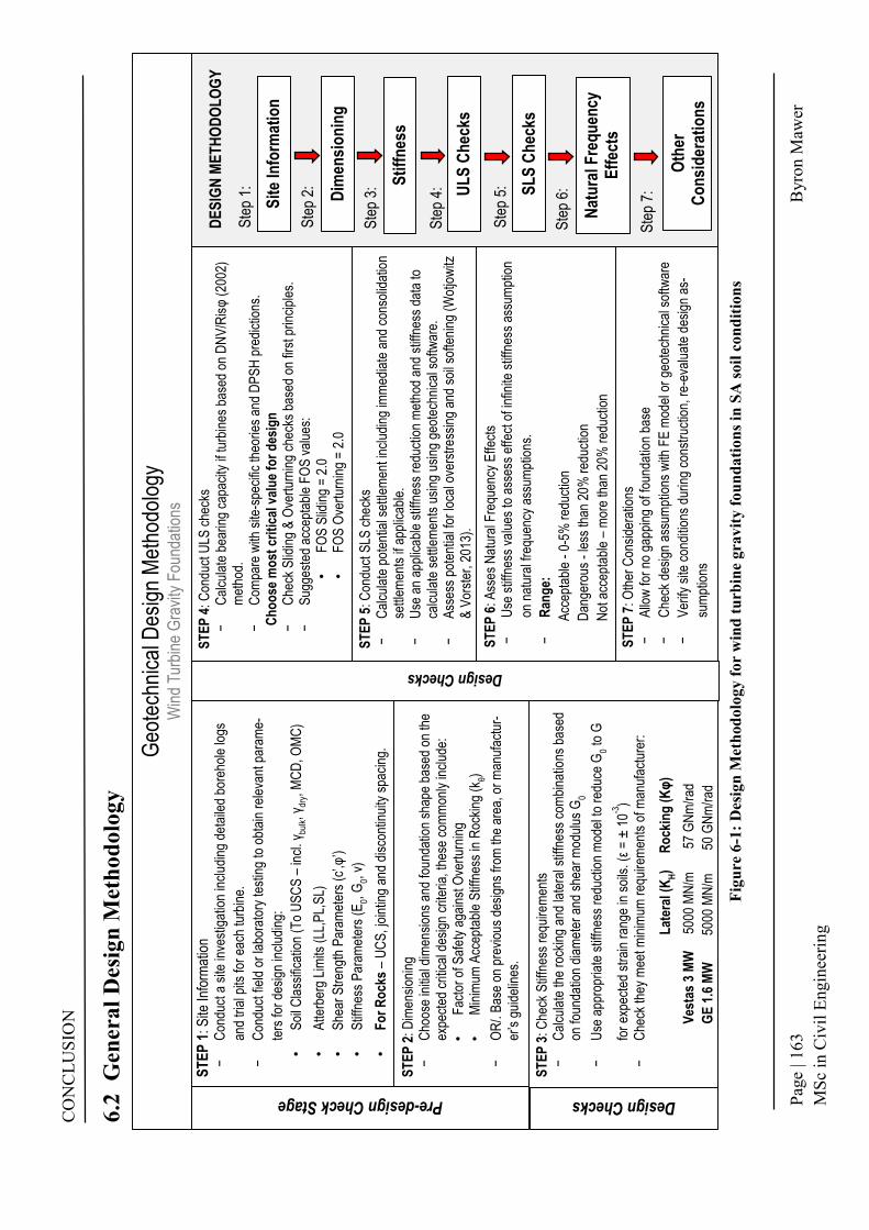
CO
NC
LUSI
ON
Page
| 16
3
B
yron
Maw
er
MSc
in C
ivil
Engi
neer
ing
6.2
Gen
eral
Des
ign
Met
hodo
logy
Figu
re 6
-1: D
esig
n M
etho
dolo
gy fo
r w
ind
turb
ine
grav
ity fo
unda
tions
in S
A so
il co
nditi
ons
ST
EP
5: C
ondu
ct S
LS c
heck
s −
Cal
cula
te p
oten
tial s
ettle
men
t inc
ludi
ng im
med
iate
and
con
solid
atio
n se
ttlem
ents
if a
pplic
able
. −
Use
an
appl
icab
le s
tiffn
ess
redu
ctio
n m
etho
d an
d st
iffne
ss d
ata
to
calc
ulat
e se
ttlem
ents
usi
ng u
sing
geo
tech
nica
l sof
twar
e.
−A
sses
s po
tent
ial f
or lo
cal o
vers
tre
ssin
g an
d so
il so
ften
ing
(Wot
jow
itz
& V
orst
er, 2
013)
.
ST
EP
1: S
ite In
form
atio
n −
Con
duct
a s
ite in
vest
igat
ion
incl
udin
g de
taile
d bo
reho
le lo
gs
and
tria
l pits
for
each
turb
ine.
−
Con
duct
fiel
d or
labo
rato
ry te
stin
g to
obt
ain
rele
vant
par
ame-
ters
for
desi
gn in
clud
ing:
•
Soi
l Cla
ssifi
catio
n (T
o U
SC
S –
incl
. γbu
lk, γ
dry,
MC
D, O
MC
) •
Atte
rber
g Li
mits
(LL
,PL,
SL)
•
She
ar S
tren
gth
Par
amet
ers
(c’,φ
’)
•S
tiffn
ess
Par
amet
ers
(E0, G
0, v)
•F
or
Ro
cks
– U
CS
, joi
ntin
g an
d di
scon
tinui
ty s
paci
ng.
ST
EP
4: C
ondu
ct U
LS c
heck
s −
Cal
cula
te b
earin
g ca
paci
ty if
turb
ines
bas
ed o
n D
NV
/Ris
φ (
2002
) m
etho
d.
−C
ompa
re w
ith s
ite-s
peci
fic th
eorie
s an
d D
PS
H p
redi
ctio
ns.
Ch
oo
se m
ost
cri
tica
l val
ue
for
des
ign
−C
heck
Slid
ing
& O
vert
urni
ng c
heck
s ba
sed
on fi
rst p
rinci
ples
. −
Sug
gest
ed a
ccep
tabl
e F
OS
val
ues:
•
FO
S S
lidin
g =
2.0
•
FO
S O
vert
urni
ng =
2.0
ST
EP
3: C
heck
Stif
fnes
s re
quire
men
ts
−C
alcu
late
the
rock
ing
and
late
ral s
tiffn
ess
com
bina
tions
bas
ed
on fo
unda
tion
diam
eter
and
she
ar m
odul
us G
0 −
Use
app
ropr
iate
stif
fnes
s re
duct
ion
mod
el to
red
uce
G0 to
G
for
expe
cted
str
ain
rang
e in
soi
ls. (
ε =
± 1
0-3)
−C
heck
they
mee
t min
imum
req
uire
men
ts o
f man
ufac
ture
r:
L
ater
al (
KH)
R
ock
ing
(K
φ)
V
esta
s 3
MW
5
000
MN
/m
5
7 G
Nm
/rad
GE
1.6
MW
500
0 M
N/m
50
GN
m/r
ad
ST
EP
7: O
ther
Con
side
ratio
ns
−A
llow
for
no g
appi
ng o
f fou
ndat
ion
base
−
Che
ck d
esig
n as
sum
ptio
ns w
ith F
E m
odel
or
geot
echn
ical
sof
twar
e
−V
erify
site
con
ditio
ns d
urin
g co
nstr
uctio
n, r
e-e
valu
ate
desi
gn a
s-
sum
ptio
ns
ST
EP
6: A
sses
Nat
ural
Fre
quen
cy E
ffect
s −
Use
stif
fnes
s va
lues
to a
sses
s ef
fect
of i
nfin
ite s
tiffn
ess
assu
mpt
ion
on n
atur
al fr
eque
ncy
assu
mpt
ions
. −
Ran
ge:
Acc
epta
ble
- 0-
5% r
educ
tion
Dan
gero
us -
less
than
20
% r
educ
tion
N
ot a
ccep
tabl
e –
mor
e th
an 2
0%
red
uctio
n
SL
S C
hec
ks
Sit
e In
form
atio
n
Dim
ensi
on
ing
Sti
ffn
ess
UL
S C
hec
ks
Ste
p 7:
Ste
p 1:
Ste
p 2:
Ste
p 3:
Ste
p 4:
Ste
p 5:
Ste
p 6:
DE
SIG
N M
ET
HO
DO
LO
GY
Nat
ura
l Fre
qu
ency
E
ffec
ts
Oth
er
Co
nsi
der
atio
ns
Design Checks
ST
EP
2: D
imen
sion
ing
−C
hoos
e in
itial
dim
ensi
ons
and
foun
datio
n sh
ape
base
d on
the
expe
cted
crit
ical
des
ign
crite
ria, t
hese
com
mon
ly in
clud
e:
•F
acto
r of
Saf
ety
agai
nst O
vert
urni
ng
•M
inim
um A
ccep
tabl
e S
tiffn
ess
in R
ocki
ng (
k θ) −
OR
/. B
ase
on p
revi
ous
desi
gns
from
the
area
, or
man
ufac
tur-
er’s
gui
delin
es.
Pre-design Check Stage
Design Checks
Geo
tech
nica
l Des
ign
Met
hodo
logy
W
ind
Tur
bine
Gra
vity
Fou
ndat
ions

RECOMMENDATIONS
Page | 164 Byron Mawer MSc in Civil Engineering
7. RECOMMENDATIONS The following recommendations are made to further pursue this field of study, improve on presented research and to further help guide South African wind turbine foundation designers in the future:
1) Further research can be conducted for various onshore wind turbine foundation types for local soil conditions. This can include pile, rock anchored or caisson designs as soil conditions are not always conducive to gravity foundations in South Africa,
2) An investigation into the design of offshore wind turbine foundation structures specifically off the southern coast, may lead to beneficial advances in the development of an offshore wind energy market for SA,
3) Design checks could be completed for wind turbine sites on less favourable soils such as clays and silts or soils dominated by soft or nodular pedocretes. This can only add to the considerations this research has already presented,
4) A gravity foundation design for SA soil conditions could be conducted using methods presented in this research in conjunction with a finite element model, to assess the strengths and weaknesses of the use of FEM in wind turbine gravity foundation design,
5) Investigating the use of resonant column or bender element laboratory testing to predict soil stiffness as an alternative to CSW testing,
6) A theoretical bearing capacity theory could be created that more accurately takes into account the occurrence of pedocrete layers to various degrees of consistency. This could be helpful for all local foundation designers not exclusively wind turbine foundation designers,
7) Settlement checks for wind turbine structures presented in this research could be expanded to include consolidation effects, as well as the assessment of the assumptions surrounding the control of differential settlement by the rocking stiffness requirements,
8) A more refined and accurate dynamic model of wind turbine soil-structure interaction could be investigated in order to further assess the infinite vs. finite soil stiffness effect on the natural frequency of the structure, and
9) This research could be furthered in the aim of producing a more comprehensive wind turbine gravity foundation guideline (similar to the DNV/Risφ guideline) suited for African soil conditions, geotechnical expertise and site investigation capabilities.

REFERENCES
Page | 165 Byron Mawer MSc in Civil Engineering
8. REFERENCES 1) Almond, J.E. (2010). Paleontological heritage assessment of the Coega IDZ, Eastern
Cape Province, 112 pp. plus appendix. Natura Viva cc, Cape Town.
2) Archer, A. (2014). Using small-strain stiffness to predict the settlement of shallow foundations on sand. MSc Dissertation. Department of Civil Engineering. University of Pretoria, South Africa.
3) Arcus GIBB Pty Ltd. (2012).Final Environmental Impact Assessment Report Submitted For Dassiesklip Wind Farm. DEA Reference: 12/12/20/1701. Available from the Department of Environmental Affairs.
4) Balmer, G. (1952). A general analytical solution for Mohr's envelope. American. Society of Testing and Materials. 52, 1260-1271.
5) Beales, P. (2012). Site Investigation Practices [Part of CIV3024S course work]. Department of Civil Engineering. University of Cape Town, South Africa.
6) Beales, P. (2015). Site Investigation Practices [Part of CIV3024S course work]. Department of Civil Engineering. University of Cape Town, South Africa.
7) Bement, R.A.P., Selby, A.R. (1997). Compaction of granular soils by uniform vibration equivalent to vibrodriving of piles. Journal of Geotechnical and Geological Engineering. 1997 (15) 121-143.
8) Bhattacharya, S. (2014). Challenges in Design of Foundations for Offshore Wind Turbines. The Institution of Engineering & Technology Reference Article. ISSN 2056-4007.
9) Bonnett, D. (2005). Wind Turbine Foundations – loading, dynamics and design. The Structural Engineer. ICE Publishing, February 2005, Pg. 41-45.
10) Bowles, J.E. (1997). Foundation analysis and design, 5th edition. McGraw-Hill Companies, Inc., Illinois, USA.
11) Brent, A. (2014). Renewable Energy in South Africa. Proceedings of the International Seminar on Design of Wind Turbine Support Structures. 3 September 2014. University of Stellenbosch, Cape Town. 1-15.
12) Brinch Hansen, J. (1970). A Revised and Extended Formula for Bearing Capacity. Denmark Geoteknisk Institut Bulletin. 28 28, 0-9.
13) Brink, A.B.A, (1979). Engineering Geology of Southern Africa - Post Gondwana Deposits. Building Publications, Pretoria, pp. 286–312.
14) Bu, D. (2005). Engineering Considerations for design of wind farm foundations. New Civil Engineer. Available at: http://www.nce.co.uk/engineering-considerations-for-design-of-wind-farm-foundations/540265.article [16 July 2015]

REFERENCES
Page | 166 Byron Mawer MSc in Civil Engineering
15) Byrne, B. (2000). Investigations of Suction Caissons in Dense Sand. Oxford University. London
16) Byrne, B. (2011). Foundation Design for Offshore Wind Turbines, Géotechnique Lecture Géotechnique ICE, London.
17) Byrne, B.W., Houlsby, G.T. (2003). Foundations for Offshore Wind Turbines. Philsophical transactions. Series A, Mathematical, physical, and engineering sciences 361, 2909–30.
18) Byrne, G., Berry, A.D., (2008). A Guide to Practical Geotechnical Engineering in Southern Africa. Franki Africa, Johannesburg, South Africa.
19) Canadian Geotechnical Society. (2006). Canadian Foundation Engineering Manual. 4th Edition. Canadian Geotechnical Society Publishing. Calgary, Canada.
20) Clayton, C. (2000). Assessing the stiffness of soils and weak rocks, Geotechnics for Developing Africa. A. A. Balkema, Rotterdam, pp. 303–315.
21) Clayton, C. (2011). Stiffness at Small Strain: Research and Practice. Geotechnique 2 61, 5–37. London.
22) Clayton, C. R. I. & Heymann, G. (2001). Stiffness of geomaterials at very small strains. Geotechnique 51, No. 3, 245-255.
23) Clayton, C. R. I., Heymann, G., Matthews, M.C., (2012). The Value of Stiffness Measured in Field Seismic Surveys. International Journal of Geo-Engineering 4(2) : 17-36
24) Clough, R.., Pienzien, J. (2003). Dynamics of Structures. Computers & Structures Inc. Berkley, USA.
25) Craig, R.F. (2004). Craig’s Soil Mechanics, 7th edition. Spon Press, Dundee, Scotland.
26) Cuelho, E., Perkins,S. (2008). Field Investigation of Geosynthetics used for Subgrade Stabilization. Made available at: http://www.mdt.mt.gov/other/research/external/docs/research_proj/subgrade/final_report.pdf Accessed on: 28 January 2015.
27) Das, B. (2009). Shallow Foundations: Bearing Capacity & Settlement. 2nd Edition. CRC Press, New York, USA.
28) Das, B. (2011). Principles of Foundation Engineering. 7th Edition. Cengage Learning, Stamford, USA.
29) Das, B., Ramana, C (2010). Principles of Soil Dynamics. 4th Edition. Cengage Learning, Stamford, USA.
30) Das, B., Sivakugan, S. (2007). Settlements of shallow foundations on granular soils - an overview. International Journal of Geotechnical Engineering, 1 (1). pp. 19-29.

REFERENCES
Page | 167 Byron Mawer MSc in Civil Engineering
31) Day, P. (2014). Wind Turbines – Geotechnical Investigations recommended practices and specifications. Proceedings of the International Seminar on Design of Wind Turbine Support Structures. 3 September 2014. University of Stellenbosch, Cape Town. 15-36.
32) Department of Energy. Renewable Energy Independent Power Producer Procurement Programme. Available at: http://www.ipprenewables.co.za/#page/303/ [20 January 2015]
33) Department of Energy. (2013). Integrated Resource Plan For Electricity (IRP) 2010-2030 – Update Report. Prepared for the Presidency of South Africa. Available at: http://www.energy.gov.za/IRP/irp%20files/IRP2010_2030_Final_Report_20110325.pdf
34) Department of Energy. (2014) Wind Energy: General. Made available at: http://www.poweredbywind.co.za/general/
35) Det Norske Veritas & Risϕ National Laboratory. (2002). Guidelines for the design of wind turbines. 2nd Edition. Det Norske Veritas. Copenhagen, Denmark.
36) Eberhard, A., Kolker,J., Leigland, J.(2014). South Africa’s Renewable Energy IPP Procurement Program: Success Factors and Lessons. Public-Private Infrastructure Advisory Facility. Washington D.C, USA.
37) European Committee for Standardization (2004) Eurocode 7: Geotechnical design - Part 1: General Rules (EN 1997-1(2004)). Brussels, Belgium
38) Gaspar, R. (2012). Concrete Wind Towers: A Low-tech Innovation for a High-tech Sector. Available at: www.renewableenergyworld.com/rea/blog/post/2012/11/concrete-wind-towers-a-low-techinnovation-for-a-high-tech-sector [April 11, 2015]
39) General Electric Report. (2013a). Load Specification for the Foundation of the Wind Turbine Generator System. GE 1.6-82.5 50 Hz 79.7m HH NAMTS IEC 2B. Document No. 109W4680.
40) General Electric Report. (2013b). Technical Specification Wind Turbine Generator Systems All Types. Document No. 109W4732.
41) Germanischer Lloyd. (2010). Guideline for the Certification of Wind Turbines. Germanischer Lloyd. Hamburg, Germany.
42) Global Wind Energy Council. (2014). Wind in numbers. Made available at: http://www.gwec.net/global-figures/wind-in-numbers/ [18 August 2015]
43) Gough, M.B. (2014) An investigation into the propagation of sinkholes using the geotechnical centrifuge. Proceedings of the 8th South African Young Geotechnical Engineers Conference. 17-19 September 2014. Stellenbosch, South Africa. 117-124.

REFERENCES
Page | 168 Byron Mawer MSc in Civil Engineering
44) Gupta, R. (2014). REIPPP in South Africa: what to expect from latest bid window. Insider PV. Available at: http://analysis.pv-insider.com/industry-insight/reippp-south-africa-what-expect-latest-bid-window [11 January 2015]
45) Hagemann, K. (2013). South Africa’s Wind Power Potential. SANEA Lecture Series. G7 Renewable Energy. Available at: http://www.sanea.org.za/CalendarOfEvents/2013/SANEALecturesCT/Feb13/KilianHagemann-G7RenewableEnergiesAndSAWEA.pdf
46) Heymann, G. (2007). Ground stiffness measurement by the continuous surface wave test. South African Institute of Civil Engineering Journal 49, 25–31.
47) Heymann, G. (2014). Report on CSW testing for Metrowind Windfarm Development. Prepared for Afri-Coast Engineers SA (Pty) Ltd. 15/10/2012.
48) Highter, W., Anders, J. (1985). Dimensioning Footings Subjected to Eccentric Loads. Journal of Geotechnical. Engineering. 111(5), 659–665.
49) Hoek, E. (1994). Strength of rock and rock masses. ISRM News Journal, 2 (2), 4-16.
50) Hoek, E., Bray, J.D. (1981). Rock Slope Engineering.3rd Edition. Taylor & Francis. New York, USA.
51) Hoek, E., Carranza-Torres, C., Corkum, B. (2002). Hoek Brown Failure Criterion – 2002 Edition. Made available as part of RocLab v1.0 software from RocScience. Vancouver, Canada.
52) International Electrotechnical Commission. (2005). IEC 61400-1 Wind Turbines Part 1 – Design Requirements. 3rd Edition. International Electrotechnical Commission. Geneva, Switzerland.
53) International Electrotechnical Commission. (2005). Wind Turbines Part 1 – Design Requirements. (IEC 61400-1 2005-08), Geneva, Switzerland.
54) Kalumba, D. (2015). Differential Settlement [CIV5110Z: Foundation Design course notes]. Department of Civil Engineering, University of Cape Town.
55) Karg, C. (2008). Modelling of Strain Accumulation Due to Low Level Vibrations in Granular Soils. PhD Dissertation. Department of Civil Engineering. Ghent University, Belgium.
56) Kassimali, A. (2015). Structural Analysis.5th Edition. Cengage Learning. Stamford, USA.
57) Kumar, S., Krishna, A., Arindam, D. 2013. Parameters affecting Dynamic Soil Properties: A review treatise. Proceeding of Indian National Conference on Recent Advances in Civil Engineering. Made available at: http://www.iitg.ac.in/arindam.dey/Publications%20Corner/2013/Kumar%20et%20al.,%20NCRACE,%202013.pdf

REFERENCES
Page | 169 Byron Mawer MSc in Civil Engineering
58) Liebherr Cranes. (n.d.). LTM Mobile Crane Technical Specifications. Made available at: http://www.liebherr.com/AT/en-GB/products_at.wfw/id-8607-0/measure-nonMetric Accessed on: 14 November 2014.
59) Lynn, P. (2012). Onshore and Offshore Wind Energy: An Introduction. John Wiley & Sons. West Sussex, United Kingdom.
60) MacRobert, C., Kalumba, D., Beales, P. (2011). Correlating Standard Penetration Test and Dynamic Probe Super Heavy Penetration Resistance Values in Sandy Soils. Journal of the South African Institution of Civil Engineering 153(1):46-54
61) Mandel, J., and Salencon, J. (1969). Force portante d’un sol sur une assise rigide, in Proceedings of 7th International Conference of Soil Mechanics and Foundation Engineering. (2) 157. Mexico City, Mexico.
62) Meyerhof, G.G. (1963). Some Recent Research on the Bearing Capacity of Foundations. Canadian Geotechnical Journal 1, 16–26.
63) Meyerhof, G. G., Hanna, A. M. (1978). Ultimate bearing capacity of foundations on layered soils under inclined load. Canadian Geotechnical Journal, 15(4): 565.
64) Morgan, K. (2008). Wind Turbine Foundation Behavior and Design Considerations. AWEA Wind Power Conference, Houston, USA. June 2008.
65) Mukasa, A., Mutambatsere, E., Arvanitis, Y., Triki, T. (2013) Development of Wind Energy in Africa. African Development Bank Group, Working Paper Series. No. 170 – March 2013.
66) Netterberg, F. (1994). Engineering Geology of Pedocrete and other Residual Soils. Proceedings of the 7th IAEG Congress, Lisbon, Portugal. September 1994.
67) Newbery, D., Eberhard, A. (2008). South African Network Infrastructure Review: Electricity. Completed for National Treasury & Department of Public Enterprises. Available at: http://www.gsb.uct.ac.za/files/SAElectricityPaper08.pdf
68) Nicholson, J. (2011). Design of wind turbine tower and foundation systems: optimization approach. Iowa Research Online. MS Dissertation. Department of Civil Engineering. University of Iowa, USA.
69) nPower & Royal Academy of Engineering. (n.d). Wind Turbine Power Calculations. Made available at: http://www.raeng.org.uk/publications/other/23-wind-turbine
70) Nordex Energy Report. (2011a). Preliminary Foundation Design N90/2500 R80 MT IEC 1b (250). Document No. PM-XEUSPC-0046.
71) Nordex Energy Report. (2011b) Specification Dynamic spring rate kphi,dyn: Foundation Design Basics. Document No. PM-XGLSPC-0057
72) Palmström , A. (1995). RMi – a rock mass characterization system for rock engineering purposes. Chapter 8. PhD thesis, Oslo University, Norway.

REFERENCES
Page | 170 Byron Mawer MSc in Civil Engineering
73) Parrock, A. (2013). Geotechnical Aspects of an Eastern Cape Wind Farm. South African Institute of Civil Engineering Magazine. April 2013: 20–25.
74) Potts, P., Zdravkovic, L. (2001). Finite Element Analysis in Geotechnical Engineering. 1st Edition. Thomas Telford. London, United Kingdom.
75) Priest, J. (2012). Chapter 24: Dynamic and Seismic Loading of Soils. ICE Manual of Geotechnical Engineering. London. United Kingdom. ICE Publishing Co. Pg. 259-269.
76) Psiorz, C. (2014). NAUE on Reinforcing Salbatica Wind Farm in Romania [Part of CIV5124Z Geosynthetic Engineering Course]. Department of Civil Engineering. University of Cape Town, South Africa.
77) Rocscience Inc. (2007). Settle 3D Theory Manual. Rocscience Inc. Made available at: https://rocscience.com/help/settle3d/webhelp/pdf_files/theory/Settle3D_Theory.pdf [14 April 2015]
78) SA Info.com. (2015). South Africa. Fast Facts. Made available at: http://www.southafrica.info/about/facts.htm#.VbIorlWqpBc#ixzz3goFgiHvG
79) Schmertmann, J.H. (1978). Use of the SPT to Measure Dynamic Soil Properties… Yes, But…!. Dynamic Geotechnical Testing, STP 654, ASTM, Philadelphia, 341–355.
80) Siemens. (2011). Wind Turbine SWT-3.0-101 / SWT-3.2-101. Made available at: http://www.energy.siemens.com/hq/en/renewable-energy/wind-power/platforms/d3-platform/wind-turbine-swt-3-2-101.htm
81) SoilLab. (2014). Geotechnical Laboratory Testing in South Africa [Lecture]. 8th South African Young Geotechnical Engineers Conference. 17-19 September 2014. Stellenbosch, South Africa
82) South African Department of Energy. (2013). IRP 2010 – 2030 Update Report. Department of Energy, Pretoria, South Africa. Available at: www.doe- irp.co.za/content/IRP2010_updatea.pdf
83) Stagg, K.G., Zienkiewicz, O.C. (1968). Rock Mechanics in Engineering Practice. John Wiley & Sons. Shepherdstown, USA.
84) Stroud, M.A. (1989) The standard penetration test: its application and interpretation. Penetration Testing in the UK, pp. 29–49, Thomas Telford, London
85) Svensson, H. (2010). Design of Foundations for Wind Turbines. MSc Dissertation. Department of Construction Studies. Lund University, Sweden.
86) The Concrete Centre & Gifford. (2007). Concrete Towers for Onshore and Offshore Wind Farms. ISBN 1-904818-48-X. Surrey, United Kingdom.
87) US Office of Energy Efficiency & Renewable Energy. (2015). Wind Turbine Basic & FAQ. Made available at: http://energy.gov/eere/energybasics/articles/wind-turbine-basics
REFERENCES
Page | 171 Byron Mawer MSc in Civil Engineering
88) Van der Tempel, J., Molenaar, D.P. (2002). Wind Turbine Structural Dynamics – A Review of the Principles for Modern Power Generation, Onshore and Offshore. Wind Engineering Volume 26, No. 4 , 2002 Pp 211–220
89) Van Zyl, W. (2014). Concrete Wind Turbine Towers. Proceedings of the International Seminar on Design of Wind Turbine Support Structures. 3 September 2014. University of Stellenbosch, Cape Town. 74-87.
90) Vestas Report. (2011). Foundations Design Guidelines: Foundations with Anchors. Document No. 0020-3286 V00. Class 2: V80/V90/V100/V112. 2011-07-08
91) Vestas Report. (2013). Foundation Loads V112 3MW 1540rpm HH 94 IEC2A. Document No. 0024-5696.V03. 2013.03.12
92) von der Haar, C. (2014). Design Aspects of Concrete Towers for Wind Turbines. Proceedings of the International Seminar on Design of Wind Turbine Support Structures. 3 September 2014. University of Stellenbosch, Cape Town. 37-46.
93) Warren-Codrington, C. (2013). Geotechnical Considerations for Onshore Wind Turbines. MSc Dissertation. Department of Civil Engineering. University of Cape Town, South Africa.
94) Way, A. (2014). A study on the design and material costs of tall wind turbine towers in South Africa. Proceedings of the International Seminar on Design of Wind Turbine Support Structures. 3 September 2014. University of Stellenbosch, Cape Town. 61-73
95) Wojtowitz, G, Vorster, E. (2014). The Design of Gravity Foundations for Wind Turbines for West Coast 1 Wind Farm. Proceedings of the 8th South African Young Geotechnical Engineers Conference. 17-19 September 2014. Stellenbosch, South Africa. 379-388.
96) Wylie, D.C. (1999). Foundations on Rock. 2nd Edition. E & FN Spon. New York, USA.)