An Introduction to GeoGebra - Mathemina/teaching/5270s13/Intro_to_Geogebra.pdfAn Introduction To GeoGebra An Introduction to GeoGebra ... as the Inverse Filling check box. It's ok

An Introduction To GeoGebra

An Introduction to GeoGebra

Steve PhelpsGeoGebra Institute of Ohio

Madeira High SchoolUniversity of Cincinnati

[email protected]

1


Table of Contents1. How to Get Started with GeoGebra ...................................................................................................................... 3

2. GeoGebra 4.0 (August 2011)................................................................................................................................. 4

3. Introduction to the GeoGebra4.0 Interface...........................................................................................................6

4. Getting to Know The Graphics View..................................................................................................................... 9

5. Changing How Things Look: GeoGebra’s Object Properties ..........................................................................11

6. Algebra 1 and Algebra 2 Things..........................................................................................................................14

7. Geometry Things.................................................................................................................................................. 27

8. Exploring Conditional Hide and Show................................................................................................................35

9. Creating Custom Tools........................................................................................................................................ 38

10. Pre-Calculus and Calculus Things..................................................................................................................40

11. Creating Dynamic Worksheets.......................................................................................................................... 47

12. Customizing the Toolbar................................................................................................................................... 49

13. Useful Links and Information: Your GeoGebra to-do List..............................................................................51

2


1. How to Get Started with GeoGebra

If you have not downloaded GeoGebra, open your browser and go to the GeoGebra Website http://www.geogebra.org.

I rarely have any problems using the WEBSTART on the networked computers at my school, nor in individual workshops with participants. However, if you are having trouble, let me know, and I will supply on off-line installer for you to use.

3


2. GeoGebra 4.0 (August 2011)

Getting to Know GeoGebra4.0

Let's begin by getting GeoGebra4.0 Beta webstarted on your laptop. This is a fully functioning version of GeoGebra, scheduled to become the official webstart version in late August (you will then follow the procedure in Section 1 to get GeoGebra4.0 started). Since it is late in the Beta testing processes, you will be working with (close) to the finished product. However, a word to the wise:

Please note that this version has many unfinished features and that all features are subject to change. GeoGebra files that you create today may not work in future versions.

Begin by opening a web browser and going to http://www.geogebra.org/forum/ . This forum is where you go to get “technical support” or “customer service.” You should spend some time reading through the Forum threads.

Scroll down towards the bottom of this page to the English: GeoGebra 4.0 Beta Forum. Click on the Forum link.

4


You want to click on the Thread Link shown below.

Click on the webstart link shown below. This will install GeoGebra4.0 Beta.

The only thing you are asked to do is to report any bugs on the GeoGebra4.0 forum. Remember! After August 21, you will follow the procedure in Section 1 to get GeoGebra4.0 started by going to the GeoGebra Website http://www.geogebra.org, clicking on the Download button, then clicking on the Webstart button on the next page.

5


3. Introduction to the GeoGebra4.0 InterfaceThe dynamic mathematics software GeoGebra provides six different views of mathematical objects as shown in the figure at right. Three of these views – the Graphics View 2, The Computer Algebra View, and the Construction Protocol – are new to GeoGebra4.0. In a nutshell, there is a lot of things you can do with GeoGebra4.0

Luckily for us, we will primarily use three of these views: a Graphics view, a, numeric Algebra view and a Spreadsheet view. These three views allow you to display mathematical objects in three different representations: graphically (e.g., points, function graphs), algebraically (e.g., coordinates of points, equations), and numerically in spreadsheet cells. Thereby, all representations of the same object are linked dynamically and adapt automatically to changes made to any of the representations, no matter how they were initially created.

6


4. Getting to Know The Graphics View

Just DRAW!

The purpose of this first activity is to practice using the Tool Bar and to get comfortable working with objects in the Graphics View.

1. To begin with, hide the Algebra View. There are three ways you can do this:

• You can go to the View Menu → Algebra,or

• Ctrl + Shift + Aor

• You can click on the small icon in the upper right corner of the Algebra View Window.

2. Next, show the Coordinate Grid . There are two ways you can do this:

• You can go to the View Menu → Grid,or

• Now that the Algebra View is closed, you can click on the small grid icon in the upper left corner.

PLAY! Draw a picture with GeoGebraUse the mouse and various tools from the Tool Bar to draw figures on the drawing pad (e.g. square, rectangle, house, tree,…). To access the tools, you must click on the small triangle to open the tools, then select the tool you want to use.

Don’t forget to read the toolbar help if you don’t know how to use a tool.

7


Things to try... • Try changing the colors and sizes of different objects.

Click on an object, then explore these mini-tools.

• Practice creating a point that lies on and object.

• Practice using the measuring tools tools

• Correct mistakes step-by-step using the Undo and Redo buttons located in the upper right corner of the window.

• Select any object and right-click (MacOS: Ctrl-click). Explore the menu that pops up.

8


5. Changing How Things Look: GeoGebra’s Object Properties Every object that you create in GeoGebra has its own PROPERTIES or attributes (color, thickness, labels, algebraic representation) that can be changed in the PROPERTIES DIALOG window.

How to access the Object PropertiesYou have already seen one way to change the object properties. Clicking on the small button in the upper right corner of the Graphics View will display an Object Properties Bar where you can change how selected objects in the Graphics View look.

9


However there are four other ways that you can access a more detailed Object Properties.

1. Right-click (MacOS: Ctrl-click) an object in either the Algebra View or Graphics View and select Object Properties OR

2. Select Object Properties… from the Edit Menu OR

3. Press Ctrl+E OR4. Double-click on an object in the Graphics

View and click on the Object Properties button.

What do the Tabs do?

Look at Steve's Circle in the image on the previous page.

Under the Basic Tab, I have selected the Circle with the name a and the caption Steve's Circle. Notice the circle command in the definition line.

Under the Color Tab, these are the available colors for any objects created in GeoGebra. Notice the history of colors used in this file.

10


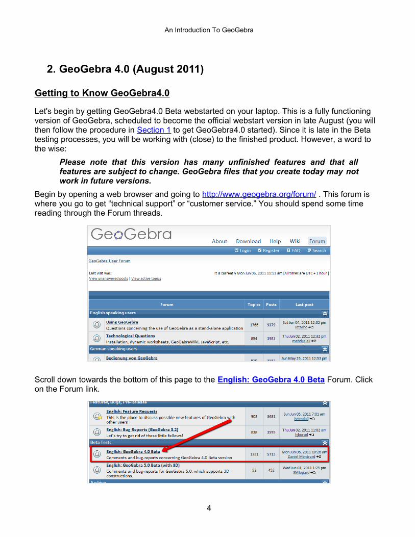
Under the Style Tab, notice how the Filling is set to 25%? You should explore the Line Style pull-down menu and the Filling Menu, as well as the Inverse Filling check box. It's ok...you will not hurt anything!

Under the Algebra Tab, the equation form can be selected.

These are the tabs that you will use most often. We will explore the Advanced Tab, time permitting. Anyone who would like to explore the Scripting Tab, I can help you individually.

Things to try... Select different objects from the list on the left hand side and explore the available

properties tabs for different types of objects. Select several objects in order to change a certain property for all of them at the same

time. Hold the Ctrl-key (MacOS: Ctrl-click) pressed and select all desired objects. Select all objects of one type by clicking on the corresponding heading. Show the value of different objects and try out different label styles. Change the properties of certain objects (e.g. color, style,…).

11


6. Some Useful ShortcutsThere are a handful of things you will do over and over in GeoGebra. Theses things are so common, that there are keyboard shortcuts to make doing this things easier. Here is a short list of useful shortcuts.

To Move the Graphics View, hold down the shift key, then click and hold and drag your mouse.

To Zoom in or out, you can scroll the scroll wheel on your mouse. This is ctrl +/– on a laptop. You can also right-click, hold, and drag a selection box in the graphics view. You will zoom in onto this box.

To Undo something you have done, you can press the key combination Ctrl-z. Often times, you will need to enter Pi in the Input Line or in some other dialogue line. You

can enter Pi by the key combination Alt-p. You can also just type the word “pi.”

Likewise, to enter a Degree symbol, use the key combination Alt-o.

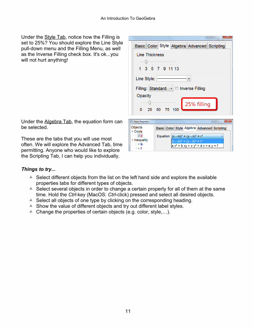
If you want to show the Coordinate Grid or the Coordinate Axes, you can View Menu → Grid, Axes. You can also use these Icon Shortcuts in the upper left corner of the graphics view.

You can also display the Algebra View, the Spreadsheet or the CAS View under the View Menu. You can also use the key combinations ctrl+shift+A, ctrl+shift+S, ctrl+shift+K, respectively.)

To change the scale on any axis, simply mover your mouse over the axis until the cursor changes into an arrow. Hold the shift key down, then click and hold and drag on the axis.

Sometimes, you may need to quickly access the lower-case Greek letters, which are used as default for angles.

Alt+A αAlt+B βAlt+D δAlt+F φAlt+G γAlt+M μ

To enter powers quickly, use the Alt key. Alt+2 is “to the second power.” Alt+6 is “to the 6 th

power.”

These are just a few of the keyboard shortcuts. Other keyboard shortcuts can be found on the GeoGebra Wiki at http://wiki.geogebra.org/en/Keyboard_Shortcuts

12


7. Algebra 1 and Algebra 2 Things

Like a Graphing Calculator

GeoGebra can be used as a graphing calculator. However, better than a graphing calculator, GeoGebra can graph implicit functions (such as x = 3) and inequalities (such as x + y < 3).

Open a new window showing the Algebra View and the Graphics View. Graph the following equations and inequalities, then graph anything of your choosing:

x ≥ 2 (x – 3)2 + y2 < 4 y ≤ x2 – 4 y > (x – 1)(x)(x + 2) x2 + x y + y2 = 1 g(x) = (x – 1)(x + 2)(x + 3)

13


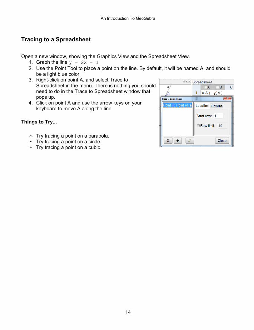
Tracing to a Spreadsheet

Open a new window, showing the Graphics View and the Spreadsheet View. 1. Graph the line y = 2x – 12. Use the Point Tool to place a point on the line. By default, it will be named A, and should

be a light blue color.3. Right-click on point A, and select Trace to

Spreadsheet in the menu. There is nothing you should need to do in the Trace to Spreadsheet window that pops up.

4. Click on point A and use the arrow keys on your keyboard to move A along the line.

Things to Try...

Try tracing a point on a parabola. Try tracing a point on a circle. Try tracing a point on a cubic.

14


Creating A Random Line

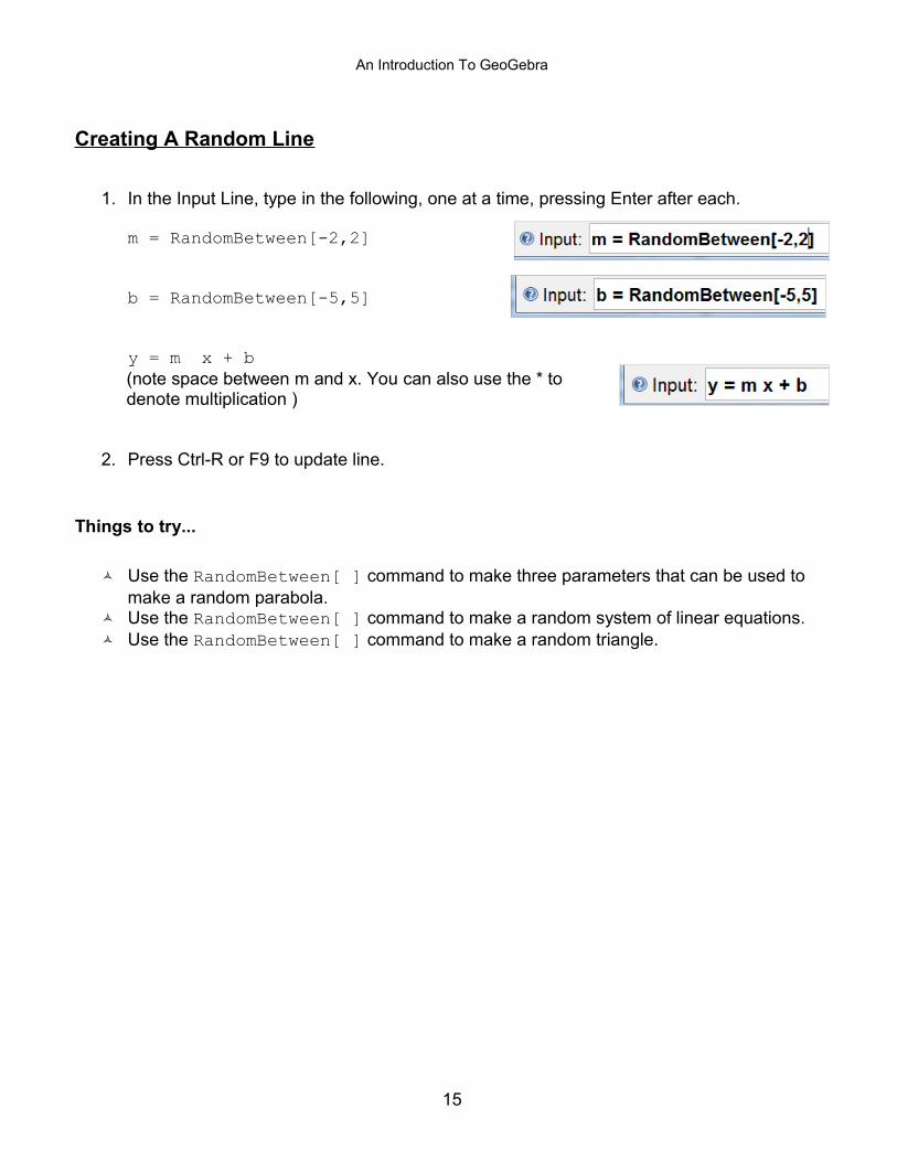
1. In the Input Line, type in the following, one at a time, pressing Enter after each.

m = RandomBetween[-2,2]

b = RandomBetween[-5,5]

y = m x + b (note space between m and x. You can also use the * to denote multiplication )

2. Press Ctrl-R or F9 to update line.

Things to try...

Use the RandomBetween[ ] command to make three parameters that can be used to make a random parabola.

Use the RandomBetween[ ] command to make a random system of linear equations. Use the RandomBetween[ ] command to make a random triangle.

15


Enhancing the Random Line

We are going to take this random line and create a Dynamic Worksheet that students could use to practice finding the equation of a line. Begin by hiding the Algebra View (View Menu → Algebra) and showing the Grid (View Menu → Grid).

1. Go to the Object Properties of the line, hide the name of the line, and make the line thicker with a brighter color (but not too bright).

2. We need to create a Text Box to show the equation of the line. To do this, activate the Insert Text Tool, and click anywhere in an open space in the Graphics View.

3. In the Text Menu that appears, click on the Object Menu, and select a, which is the name of the line. Click OK.

4. Repeatedly press CTRL+R to create a new random line. Notice that the equation of the line is dynamic, and changes, too.

5. Of course, this would not be a very good activity for our students if they could just SEE the equation. We need to create a Check Box that students can click on to Show and Hide the answer. Begin by activating the Check Box Tool, and clicking in an open space in the Graphics View.

16


6. In the Check Box window that appears, give your Check Box a name (Caption), and select the objects you want to be controlled by the Check Box by either clicking on the objects in the Graphics View, or by using the Pull-down menu to select the object. Play with your random line and the check box!

7. In anticipation of creating our Dynamic Worksheet, reduce the size of your window, move the check box and text close together, and make sure you UNCHECK the check box.

17


Creating a Dynamic Worksheet

A Dynamic Worksheet is a webpage with a GeoGebra Applet that students interact with. You need to do nothing special. Creating this webpage is as easy as saving your GeoGebra file.

1. To create a Dynamic Worksheet, go to the File Menu → Export → Dynamic Worksheet as Webpage. A window like the one below will appear.

2. After you have filled in the Title, Author (YOU), and any text or instructions you would like to appear on the webpage, click on the Advanced Tab.

3. Save the file somewhere where you will find it easily!

18


4. The finished product. Upload this file to your teacher webpage, wiki, or blog.

19


Linear Programming

Linear programming is a staple of Algebra 2 curricula. GeoGebra can be used to explore the solutions of these problems with its dynamic capabilities.

Consider the problem from http://www.purplemath.com/modules/linprog3.htm .

A calculator company produces a scientific calculator and a graphing calculator. Long-term projections indicate an expected demand of at least 100 scientific and 80 graphing calculators each day. Because of limitations on production capacity, no more than 200 scientific and 170 graphing calculators can be made daily. To satisfy a shipping contract, a total of at least 200 calculators much be shipped each day.

If each scientific calculator sold results in a $2 loss, but each graphing calculator produces a $5 profit, how many of each type should be made daily to maximize net profits?

Let x be the number if scientific calculators produced, and y be the number of graphing calculators produced.

The constraints are as follows:

x > 100y > 80 x < 200y < 170

x + y > 200

I want to maximize -2x + 5y subject to the given constraints.

Let's solve this using GeoGebra.

1. Begin by showing the Algebra View, the Graphics View, and the Spreadsheet View. Show the Coordinate Axes.

2. We need to change the scales on the axes and label the axes. To do this, we need to access the Object Properties of the Graphics View. You can do this in one of two ways: You can go to the Options Menu → Settings... , or you can right-click in on open space in the Graphics View and select Graphics... in the context menu that pops up.

20


3. Regardless of the method you use to access the Graphics settings, click on the Graphics tab at the top of the window. Make sure you click on the Basic tab underneath that tab. Use these window settings as a place to start. We can customize our window settings later.

4. Click on the xAxis tab, and make the changes shown in the figure.

5. Click on the yAxis tab and make the same types of changes there.

Under both of these tabs, you may want to consider checking the box Positive Direction Only, but this is a personal preference.

Do not worry about the Grid Tab. There is nothing we need to change for this problem.

6. Click CLOSE when finished making desired changes.

7. In the Input Line, type in the following constraints:

100 < x < 200

80 < y < 170

x + y > 200

21


8. All of your inequalities are shaded the same color. To change how the different regions are shaded, we need to access the Object Properties of each region. With all of these overlapping regions, I find it easiest to right-click on the object in the Algebra View, and selecting Object Properties from the context menu.

9. You can change the color of the regions under the COLOR tab. You can change the shading of the regions under the STYLE tab. Explore this different settings for the shadings. Click CLOSE when finished making your changes.

10.Place a point somewhere in an open space in the graphics view, NOT in one of the shaded regions. By default, this should be labeled A. Access the object properties, and change the Labeling property to Value.

11. In the Input Line, enter A1 = -2 x(A) + 5 y(A). Drag point A around the feasible region, confirming that the maximum value occurs at (100, 170).

22


Linear Programming (An Alternative Solution)

Some folks will not care for graphing the inequalities, and will rather the students construct the feasible region. Here is another way to solve this problem.

1. Use the same settings as before. Graph each of the following equations one at a time.

x = 100, y = 80 , x = 200, y = 170, x + y = 200

2. Use the Intersection Point Tool to construct the vertices of the feasible region.

3. Use the Polygon Tool to construct the feasible region. You can also use the command POLYGON[ A, B, C, D, E ]

4. Use the Point on Object Tool to place a point inside the feasible region. By default, this point will be labeled F. You will be able to drag this point, but it can not be removed from the feasible region.

5. In the Input Line, enter A1 = -2 x(F) + 5 y(F). Drag point F around the feasible region, confirming that the maximum value occurs at (100, 170).

23


Changing Parameters Using Sliders

Creating SlidersOne of the beautiful things about GeoGebra is the ease with which you can create a slider. Another beautiful thing about GeoGebra is that any command that takes a number as an input (for example: Circle[point, radius] or Polygon[point, point, number of sides] )can be controlled by a slider.

There are two ways to create a slider:

1. Begin by activating the Slider Tool. To use the tool, click anywhere is an open space in the graphics view.

In the window that appears, give your slider a name (no spaces). If you are using the slider to control a rotations, select the Angle button. Determine the interval for your slider. Under the SLIDER tab, you can control the size of the slider.

2. Another way to create a slider is by entering the name of the slider in the Input Line and pressing Enter. The slider will appear in the Algebra View. Click on the small empty circle to un-hide the slider. Once you have created the slider, explore its object properties.

Things to Try...

Create a slider n then enter each of these in the input line:

Circle[(1,2) , n] Polygon[(0,0), (1,-1), n] TaylorPolynomial[ sin(x), 1, n] ( n , n2 )

24


Parameters of a Linear Equation

You have already created a file that produces a line with a random slope and a random y-intercept, enhanced the file by adding color, a text box, and a check box, then created a Dynamic Worksheet for your students to practice. We will now create a file that can be used for the INSTRUCTION of writing equations of lines.Begin by opening a new GeoGebra file. Showi the Algebra View and the Graphics View. Show the Grid and the Axes in the Graphics View.

1. Create sliders m and b.2. In the Input Line, enter line: y = m * x + b

Drag the sliders and observe the changes in the graph of the line.

Enhancing the Construction

3. Create the intersection point of the line and the y-axis by activiating the intersection point tool, then clicking on the line and the y-axis. You can use the command Intersect[line, yAxis]. By default, this will be named A.

4. Construct a point at the origin. By default, this will be named B.

5. Construct a segment from A to B. Use the segment's Object Properties to make the segments thicker, more colorful, and to have only its VALUE show as it label.

6. Use the Slope Tool to show the slope triangle for the line.

7. Hide any unwanted points or unnecessary objects.

8. Add a Text Box that will show the equation of the line.

Things to Try... Some folks do not like the slope triangle. Try to construct

your own! Export this file to a Dynamic Worksheet. Go back to Step #2 and enter line: f(x) = m * x + b. Then open up the

Speadsheet View and create a list of function values. Right-click on a slider, and select Animation On.

25


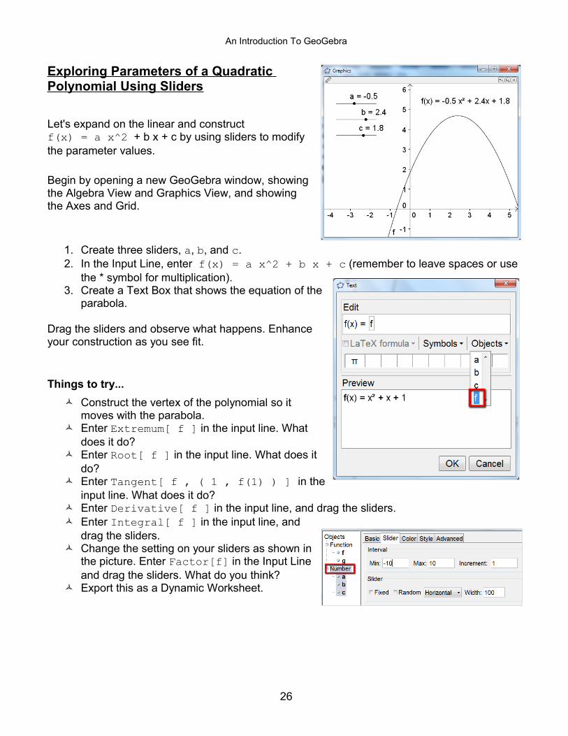
Exploring Parameters of a Quadratic Polynomial Using Sliders

Let's expand on the linear and construct f(x) = a x^2 + b x + c by using sliders to modify the parameter values.

Begin by opening a new GeoGebra window, showing the Algebra View and Graphics View, and showing the Axes and Grid.

1. Create three sliders, a, b, and c.2. In the Input Line, enter f(x) = a x^2 + b x + c (remember to leave spaces or use

the * symbol for multiplication).3. Create a Text Box that shows the equation of the

parabola.

Drag the sliders and observe what happens. Enhance your construction as you see fit.

Things to try... Construct the vertex of the polynomial so it

moves with the parabola. Enter Extremum[ f ] in the input line. What

does it do? Enter Root[ f ] in the input line. What does it

do? Enter Tangent[ f , ( 1 , f(1) ) ] in the

input line. What does it do? Enter Derivative[ f ] in the input line, and drag the sliders. Enter Integral[ f ] in the input line, and

drag the sliders. Change the setting on your sliders as shown in

the picture. Enter Factor[f] in the Input Line and drag the sliders. What do you think?

Export this as a Dynamic Worksheet.

26


Graphing a Polynomial Using Roots

It may be useful to graph a polynomial using it roots. Open a new window. Show the Algebra View and the Graphics View. Show the coordinate axes.

1. Use the point tool to place three points on the x-axis. By default, these points will be labeled A, B, and C.

2. In the input line, enter f(x) = ( x – x(A) ) ( x – x(B) ) ( x – x(C) ) .

3. You may need to change the scale of the y-axis by clicking, holding, and dragging the y-axis until you can see the entire graph.

Things to Try...

• Enhance your construction by adding color, line thickness, and a text box that displays the function equation.

• Try the command Expand[ f(x) ] and display the result in a text box in the Graphics View.

• Create a quartic with four roots.

• Create a quadratic using roots, and construct the line of symmetry.

• Try some of these commands: Extremum[f(x)] and InflectionPoint[f(x)]

27


Creating a Factoring Practice Applet

Every student in Algebra 1 will need to practice factoring quadratics at some time or another. The following steps will walk you through how to create your own “Factoring Practice” applet.

Our strategy will be as follows: We will create two random integers, a and b. We will use these random integers in the product (x + a)(x + b) = x2 + (a + b)x + ab

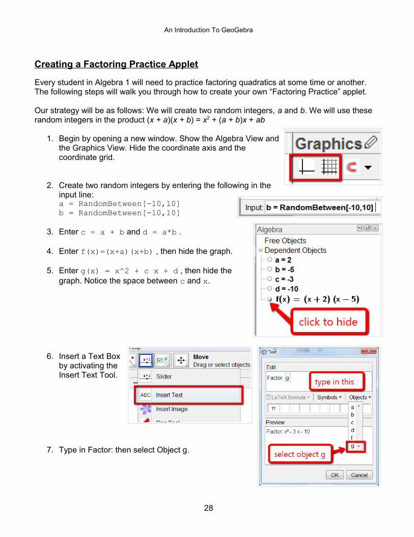
1. Begin by opening a new window. Show the Algebra View and the Graphics View. Hide the coordinate axis and the coordinate grid.

2. Create two random integers by entering the following in the input line: a = RandomBetween[-10,10]b = RandomBetween[-10,10]

3. Enter c = a + b and d = a*b .

4. Enter f(x)=(x+a)(x+b) , then hide the graph.

5. Enter g(x) = x^2 + c x + d , then hide the graph. Notice the space between c and x.

6. Insert a Text Box by activating the Insert Text Tool.

7. Type in Factor: then select Object g.

28


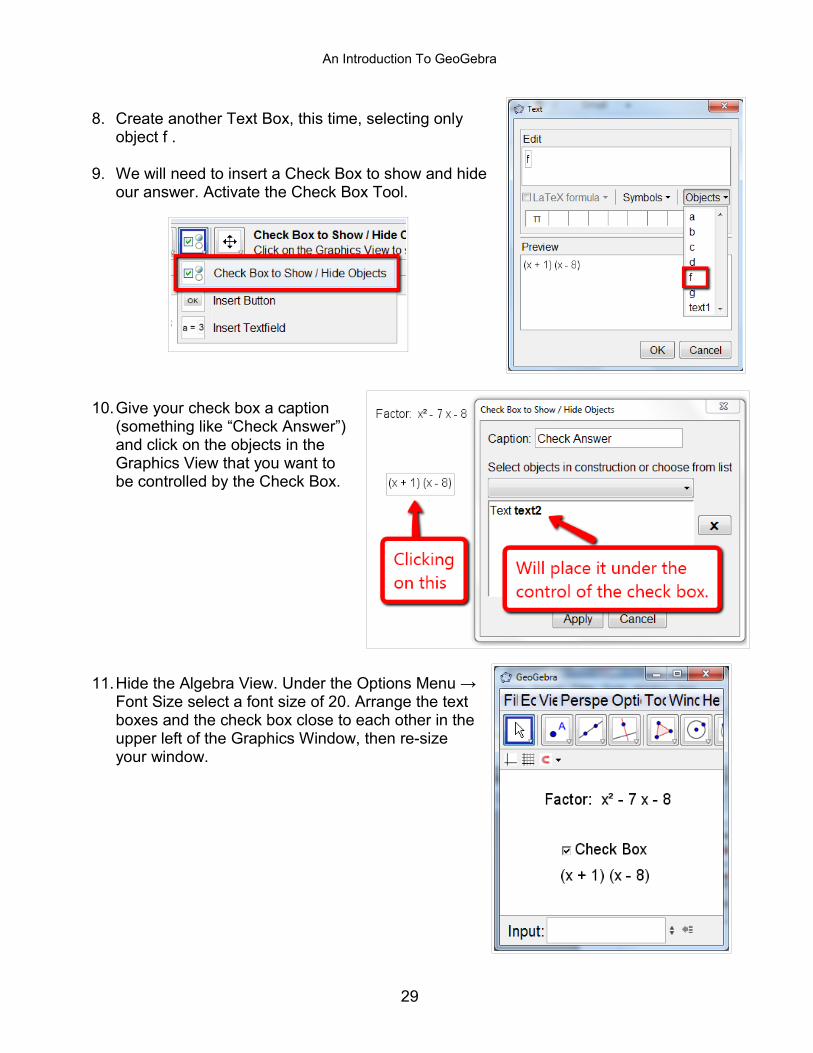
8. Create another Text Box, this time, selecting only object f .

9. We will need to insert a Check Box to show and hide our answer. Activate the Check Box Tool.

10.Give your check box a caption (something like “Check Answer”) and click on the objects in the Graphics View that you want to be controlled by the Check Box.

11.Hide the Algebra View. Under the Options Menu → Font Size select a font size of 20. Arrange the text boxes and the check box close to each other in the upper left of the Graphics Window, then re-size your window.

29


12.Uncheck the Check Box so your answer is hidden. Export this file to a Dynamic Worksheet. Type instructions in the box that will appear above the applet.

13.Click on the Advanced Tab. The only thing you should check on this page is the Show Icon to Reset Construction.

14. Save the resulting html file somewhere where you can find it easily. This file is what you would upload to your teacher webpage or wiki.

Things to Try...

• Modify this so the leading coefficient is not 1.

• Modify this so it is a Factoring a Difference of Two Squares practice, or a Factoring a Perfect Square Trinomial Practice.

• Modify this so it is Factoring a Difference off Two Cubes practice.

30


Creating a Factoring Applet: A Different Way

1. Open a new GeoGebra window. Show the Algebra View and the Graphics View. Hide the coodinate axes.

2. Create two random integers a and b as before.

3. Create the function f(x) = (x+a)(x+b), and hide the graph as before.

4. Create the function g(x) = simplify[ f(x) ], and hide the graph as before.

5. Continue as before from Step 6.

31


The Sequence Command

If the Algebra View is not open, open it by View Menu → Algebra

1. Type each of these commands one at a time in the Input Line, pressing Enter after each. BE CAREFUL TYPING THISE IN! LOOK OUT FOR COMMAS! Study carefully what is happening!

Sequence[2n + 1, n, 1, 10]

Sequence[(a, a2), a, 1, 10]

Sequence[Sequence[(i,j),j,1,i],i,1,10]

2. Let's create a Limaçon. Type each of these commands one at a time in the Input Line, pressing Enter after each.

A=(2, 0)

Sequence[Circle[( sin(i), cos(i) ), A], i, 0, 2π, 0.1]

3. Move A to (1, 0) for a cardioid.

Things to try...Play around with these sequences by making changes to the numbers.

Sequence[ Polygon[ (0,0) , ( 1,0) , n ] , n , 3 , 10 ] Sequence[ Circle[ (0,0) , r ] , r , 1 , 5 , 0.25] Sequence[ TaylorPolynomial[ sin(x) , pi , n ] , n , 1 , 5 ] Sequence[ Derivative[ x + x³ + x² + x + 1 , n ] , n , 1 , 4 ]⁴ Sequence[x² + c, c, -5, 5, 0.5] Sequence[x² + c x, c, -5, 5, 0.5] Sequence[c x² - 1, c, -5, 5, 0.5]

32


Library of Algebraic Functions

Apart from polynomials there are different types of functions available in GeoGebra (e.g. trigonometric functions, absolute value function, exponential function). Functions are treated as objects and can be used in combination with geometric constructions.

To access the list of function, click on the list icon in the lower left corner of the window.

You can click on the individual function you wish to use, you you can just type it in yourself. To close the function window, just click on the list icon again.

Excursion into Physics: Superposition of Sine WavesSound waves can be mathematically represented as a combination of sine waves. Every musical tone is composed of several sine waves of form y ( t)=a⋅sin (ω⋅t +φ )

The amplitude a influences the volume of the tone while the angular frequency ω determines the pitch of the tone. The parameter φ is called phase and indicates if the sound wave is shifted in time.

If two sine waves interfere, superposition occurs. This means that the sine waves amplify or diminish each other. We can simulate this phenomenon with GeoGebra in order to examine special cases that also occur in nature.

The lower case Greek Letters and other special symbols can be found in the Input Line when you begin to type.

To insert a subscript, use an underscore.

33


Graphing Trig Functions

Open a new widow, show the Algebra View and the Graphics View.

1. Begin by creating three sliders: a_1, ω_1, and φ_12. Enter the sine function: g(x)= a_1 sin(ω_1 x + φ_1)3. Create three more sliders: a_1, ω_1, and φ_14. Enter another sine function:

h(x)= a_2 sin(ω_2 x + φ_2)5. Create the sum of both functions:

sum(x) = g(x) + h(x)

Next, we want to change the axes so they work better with Trig Functions. Right-click in on open space, and in the menu that appears, select Graphics...

In the Graphics Properties, click on the xAxis Tab, then in the Distance pull-down menu, select π/2.

This is a GREAT time to explore this window!

Things to Try… Add a text box that displays the two sine graph equations as well as their sum. Examine the impact of the parameters on the graph of the sine functions by changing the

values of the sliders. Set a1 = 1, ω1 = 1, and φ1 = 0. For which values of a2, ω2, and φ2 does the sum have

maximal amplitude? For which values of a2, ω2, and φ2 do the two functions cancel each other?

34


Solving Equations with CAS

A Computer Algebra System (CAS) can be a powerful way for students to learn how to solve equations.

1. Begin by opening a new GeoGebra window. Show the CAS View be View Menu → CAS. This view will open in a new window. Type in your favorite linear equation in one variable, and click on the equal button.

2. Enter the left parentheses in Line 2 (both right and left parentheses will appear), then click on the equation you entered in Line 1. This will insert the equation into Line 2 inside the parentheses.

3. Perform the operation, clicking on the equal button.

4. Continue step-by-step until you reach a solution.

Things to Try...

What are some of the common mistakes students make when solving equation? How can CAS help students to see the error of their ways?

Explore solving other equations, or some of the other tools.

35


8. Geometry Things

Plotting a Graph of Two Variables

Let's construct an equilateral triangle and plot a graph of the area vs. the side length.

1. Begin by opening a new GeoGebra window. Show the Algebra View, the Graphic View, and the GRAPHICS 2 VIEW. Set the Labeling Options to NEW POINTS ONLY. Show the Coordinate Axes in Graphics View 1. Hide the Coordinate Axes and Grid in Graphics View 2.

2. Click in the Graphics 2 View. Use the Point Tool to construct two points . By default, they will be labeled A and B.

3. Activate the Regular Polygon Tool. Click on points A and B. Enter the number of sides in the window that pops up.

36


4. In the Algebra View, the sides of the equilateral triangle as displayed as a, b, and c. The area of the triangle is displayed as poly1.

5. Click in the Graphics 1 Window. Look for the PENCIL icon to be displayed in header of the window.

6. In the Input Line, enter P = ( c , poly1 ) .

7. Right-click on point P in the Graphics 1 Window, and select TRACE ON from the context menu.

8. Click on Point A or B in the Graphics 2 Window, and use the mouse or the arrow keys to move one of these points around your screen.

9. Click in the Graphics 1 Window. In the Input Line, enter Area(x) = 0.25 sqrt(3) x² .

Things to Try...

• Add a slider n in Graphics View 1. Graph the equation Area(x) = n sqrt(3) x². Use the slider to help you match the graph.

• Explore Area v. Side Length graphs for other regular polygons.

• Show the Spreadsheet View and generate some Area(x) values.

• Export this to a Dynamic Worksheet.

37


Changing the Steps in a Construction: The Construction Protocol.

Lets construct a rectangle, and then explore how we might be able to change the order of the steps in the construction using something called The Construction Protocol.

1. Open up a new window, hiding the Algebra View, the Coordinate Axes, and the Grid. Set Labeling options to All New Objects. You can do this under the Options Menu. Make sure Point Capturing is set to Automatic.

2. Use the Segment tool to construct a segment. By default, the endpoints will be A and B, and the segment label will be a.

3. Use the Perpendicular Line Tool to construct a perpendicular to the segment AB at point B. You could also use the command PerpendicularLine[ B , a ]. By default, this line will be named b.

4. Construct a Perpendicular line to segment AB through point A. This line will be named c.

5. Place a point on line b. You could use the tool, but try the command C=Point[b].

6. Construct a line perpendicular to line b through point C. This line will be named d.

7. Construct the intersection point of lines c and d. You can use the intersection point tool by clicking on the two objects that intersect, or you can use the command Intersect[ c, d ]. This point will be named D.

8. Hide lines b, c, and d. Construct the sides of the rectangle using the segment tool.

9. Show the Construction Protocol by View Menu → Construction Protocol. You can play through your construction step-by-step. Try to click on a step and drag it to another spot in the list, then play through the construction again.

38


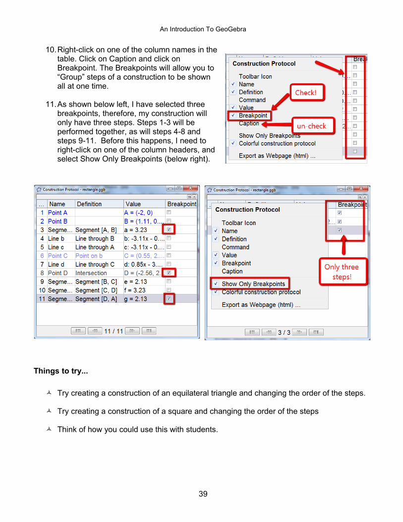
10.Right-click on one of the column names in the table. Click on Caption and click on Breakpoint. The Breakpoints will allow you to “Group” steps of a construction to be shown all at one time.

11.As shown below left, I have selected three breakpoints, therefore, my construction will only have three steps. Steps 1-3 will be performed together, as will steps 4-8 and steps 9-11. Before this happens, I need to right-click on one of the column headers, and select Show Only Breakpoints (below right).

Things to try...

Try creating a construction of an equilateral triangle and changing the order of the steps.

Try creating a construction of a square and changing the order of the steps

Think of how you could use this with students.

39


Polygons and Pi

Begin by turning off the labeling. Go to Options Menu → Labeling → No New Objects

1. Create point A=(0,0) and point B=(1,0).

2. Draw a circle Circle Tool with center A and radius point B or by using the command Circle[ A, B ]. You may want to adjust your axis scale by zooming in.

3. Use the Slider Tool to create a slider n with increment 1. Activate the tool, click in an open space, then modify the slider menu as shown.

4. Rotate B about A by angle 360°/n. You can use the Rotate Tool, or you can type in the command Rotate[B, 360°/n, A] into the Input Bar. Remember Alt+o.

5. Use the Regular Polygon Tool to create a Regular Polygon with with n sides using points B and B', or you can enter the command Polygon[B,B',n]

6. Use the Text Tool by clicking in an open space and typing in “ Area of Polygon = ” then selecting poly1 on the Objects menu.

7. Change the rounding by Options Menu → Rounding → 10 decimal places.

Things to Try...

Export this to a Dynamic Worksheet

40


Transformation by Matrices

If the Spreadsheet View is not open, open it by View Menu → Spreadsheet View.

Set the labeling properties to label New Points Only. Object Menu → Labeling → New Points Only.

1. Type the following into the Input Line one at a time:

A=(1,0) B=(0,1) A1=x(A)

A2=y(A) B1=x(B) B2=y(B)

2. Select cells A1, A2, B1, B2. Right click in one of the cells, then select Create Matrix.

3. Use the Polygon Tool to draw a Triangle CDE.

4. Type the following into the Input Line one at a time.

C' = matrix1 C

D' = matrix1 D

E' = matrix1 E

Polygon[C', D', E']

Polygon[ (0,0), A, A + B, B]

Be certain to drag points A and B around and observe the changes.

Things to Try...

GeoGebra will operate on Matrices. Create another matrix and explore which operations you can perform.

41


Transformations Using Images

Inserting an Image in GeoGebraWith GeoGebra, users have had the ability to insert images into the Graphics View for many years. In order to insert an image, be certain you have an image saved on your computer to use. I find students like to see my picture distorted!

To insert an image, begin by activating the Insert Image Tool. Click in on open space in the Graphics View. This will set the lower left corner (corner 1) of your image

When you insert an image, the corners are numbered counterclockwise beginning with the lower left corner.

By attaching the corners to Free Points in the Graphics View, you can easily distort the image as shown below. You can do this by going to the position tab in the Image Object Properties. Right-click on the image to go to the Object Properties.

42


Resizing, Reflecting, and Distorting a Picture

In this activity you will to learn how to resize an inserted picture to a certain size and how to apply transformations to the picture in GeoGebra.

1. Begin by finding a picture online and saving it somewhere where you can easily find it.

2. Open a new GeoGebra window and hide the Algebra View.3. Insert the picture using the Insert Picture Tool.4. Place a point A somewhere in the Graphics View. Set this as

CORNER 1 of your image.

5. In the Input Line, type in B = A + (3, 0). This will create point B 3 units to the right of point A. Set point B Corner 2.

6. Use the Line Tool to construct a line. 7. Use the Reflect Object about Line tool to reflect the image

across the line (Click on the image, then the line).

8. Access the Object Properties of the reflected image, and change the Opacity of the image to something less than 100. Explore the Filling pull-down menu while you are here!

Things to Try… Move point A with the mouse. How does this affect the picture? Move the picture with the mouse and observe how this affects its image. Move the line of reflection by dragging the two points with the mouse. How does this

affect the image? How can you use this construction to demonstrate something NOT being symmetric? Add point C = A + (0,4). What does this do to the construction. Go back to the Transformations by Matrices and add images to the construction. Insert an image and try to graph equations that match the image.

43


Translating Images

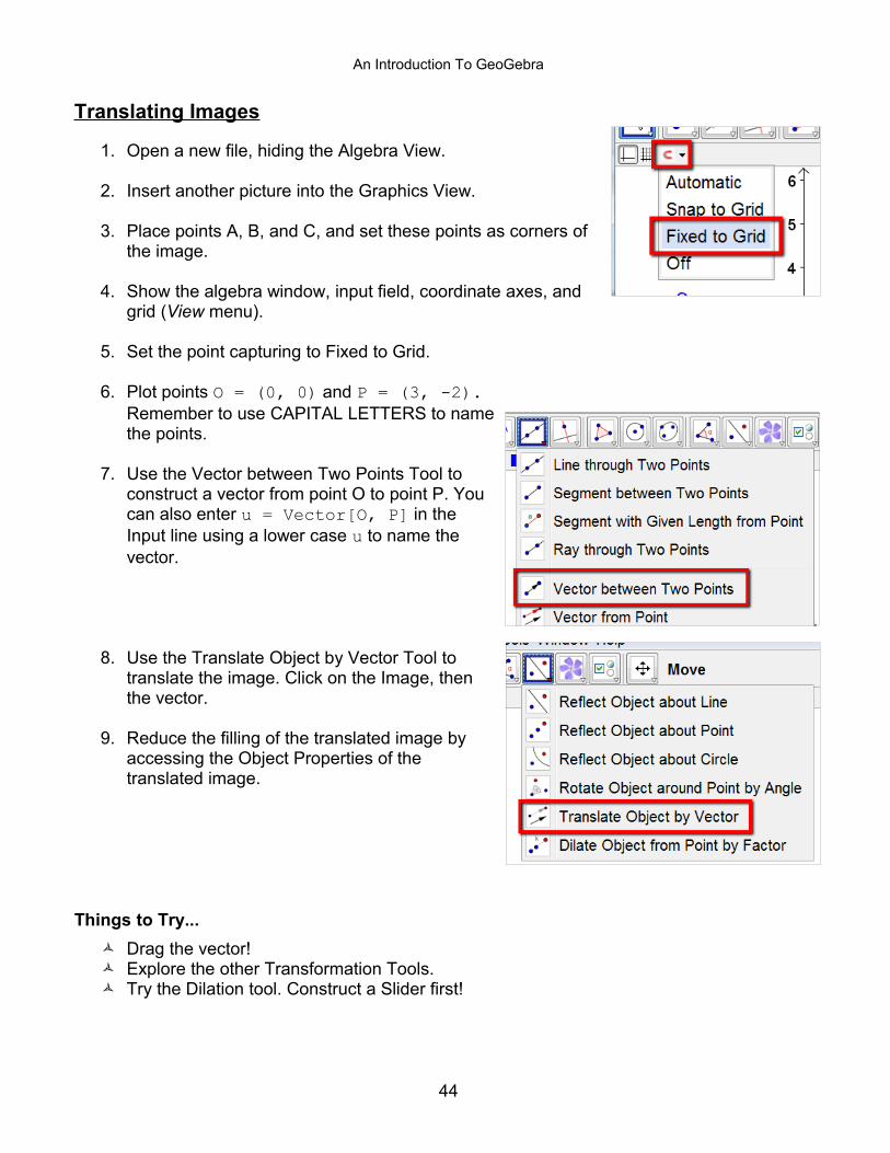
1. Open a new file, hiding the Algebra View.

2. Insert another picture into the Graphics View.

3. Place points A, B, and C, and set these points as corners of the image.

4. Show the algebra window, input field, coordinate axes, and grid (View menu).

5. Set the point capturing to Fixed to Grid.

6. Plot points O = (0, 0) and P = (3, -2). Remember to use CAPITAL LETTERS to name the points.

7. Use the Vector between Two Points Tool to construct a vector from point O to point P. You can also enter u = Vector[O, P] in the Input line using a lower case u to name the vector.

8. Use the Translate Object by Vector Tool to translate the image. Click on the Image, then the vector.

9. Reduce the filling of the translated image by accessing the Object Properties of the translated image.

Things to Try... Drag the vector! Explore the other Transformation Tools. Try the Dilation tool. Construct a Slider first!

44


Rotating Images Using a Slider

1. Begin by opening a new GeoGebra window, hiding the Algebra View, setting the Labeling Options to New Points Only. Show the Axes and the Grid.

2. Use the Polygon Tool to draw an object. I like to use the letter F because it is easier for students to see the orientation. Use the Point tool to place a point anywhere.

3. Use the Slider Tool to insert a slider by clicking in an open space in the Graphics View.

4. In the Slider window that opens, select the Angle Button, give your slider a name (something better than the default α), and change the increment to 45°.

5. Activate the Rotate Object tool. You will click on the Object you want to rotate (the F), then the center of rotation (point K), and then you will be prompted to enter an angle. Just type the name of your slider and select Counterclockwise.

Things to Try...

Export this to a Dynamic Worksheet. Change the slider to rotate in 90° increments.

45


Dilating Images using a Slider

1. Begin by inserting an image, and attaching the image to three points.

2. Construct a slider. Name it ScaleFactor.

3. Place another point somewhere close to the image, but not on the image. By default, this point will be labeled D. After you put the Point Tool away, rename it by clicking on the point and typing the name Center.

4. Activate the Dilate Object from Point by Factor tool. To use it, Click on the Image, then Click on the point CENTER, then in the window that pops up, type in the name of the slider.

Things to Try...• Reduce the Filling of the dilated image.• Combine two translations and explore when they are equivalent.

46


9. Exploring Conditional Hide and ShowThis is something that can be anywhere. We will walk through a couple of examples that will show you how to make objects appear and disappear based on some other object.

1. Begin with a new GeoGebra window. Show the Algebra View and the Graphics View. Leave the coordinate axes visible.

2. Place Point A somewhere in the First Quadrant. Change the properties of Point A so that it is BIG and Colorful! Also, have the coordinates of the point show, too.

3. Place a text box in each quadrant by entering in the Input Line Q1 = Text[ “Quadrant I” ] . You will need to drag this text box up into the first quadrant.

4. Repeat this for the remaining Quadrants. You should have something that looks like the figure at right.

We want to have each text box appear only when Point A is located in that quadrant. In GeoGebra terms, we want the Text Box named Q1 to appear when x(A) > 0 and y(A) > 0.

5. Access the Object Properties of text box Q1. Under the Advanced Tab, enter x(A) > 0 && y(A) > 0 in the Conditions to Show Object line. The && mean Logical AND in GeoGebra.

6. Repeat this for each of the other text boxes, entering the appropriate conditions for each.

Things to Try...

Export this to a Dynamic Worksheet. Add two more text boxes that will display when Point A is on the x-axis or y-axis. Instead of text boxed, make images that will hide and show based

on the position of point A.

47


Self-Checking Reflected Point

These steps will walk you through the construction of a file that kids could use to practice identifying the reflection of a point in a line.

1. Begin by Opening a new GeoGebra file. Hide the Algebra View. Set point capturing to Fixed on Grid. Set labeling options to New Points Only by Options Menu → Labeling → New Points Only.

2. In the Input Line, enter A = (RandomBetween[-5,5], RandomBetween[-5,5]).

3. Plot point B anywhere you like.

4. Construct point C by C = (RandomBetween[-2,2], RandomBetween[-2,2])

5. Construct point D by D = C + (1,0).

6. Construct point E by E = Rotate[D, RandomBetween[0, 3] 45°, C] (Alt+o for the degree symbol)

7. Construct a line using the command Line[ C , E ].

8. Reflect Point A over this line. By default, it will be named A'.

9. Hide points A', C, D, and E. Press CTRL+R a couple of times so you can see how things change.

10. In the Input Line, type the command Text[ “ Good Work! “ ] , then drag the resulting text off to the side of the window.

11. In the Input Line, type the command Text[ “ Keep Trying! “ ] , then drag the resulting text off to the side of the window.

12. Insert a Check Box. In the window that pops up, just give your Check Box a caption (Check Answer).

48


13. Access the Object properties of the Text Box that says Good Work!. Go to the Advanced Tab.

In the Conditions to Show Object line, type in A'= =B && a . Typing = = is how you test for two things to be equal. Typing in && is the logical AND.

By typing this, we are telling the text box to appear only when point B is dragged to point A', and when the Check Box is checked. DO NOT CLOSE THE WINDOW YET!

14.Click on text2 on the left side of the Object Properties window, and enter A'!=B && a for the Condition to Show Object. Can you guess what != means?

Things to Try...

Change the random coordinates or the points, or change how the line behaves.

Instead of showing a text box, show a smiley face or a frowny face image.

Make a file the will allow students to practice random rotations of 90°, 180°, and 270°. This command might be helpful E = Rotate[D, RandomBetween[1, 3] 90°, C]. Then you just want to drag A to E.

Make a text box that shows the equation of a random line. Have a line that you drag to match the equation. Have a smiley face image appear when you are correct!

49


Conditional Coloring

You are going to construct a circle and one point that is not the center or radius point of the circle.. Depending where the point is located with respect to the lines will determine the color of the point.

1. Begin by opening a new window. Show the Algebra View and the Graphics View. Hide the coordinate axes. Set the Labeling Options to New Points Only.

2. Use the Circle Tool to construct a circle. By default, the center will be labeled A and the radius point will be labeled B.

3. Use the point tool to construct a point the is not on the circle. This circle will be labeled C.

4. Access the Object Properties of point C. Click on the Advanced Tab. In the Dynamic Colors, type in AC > AB in the Red Line, and AC < AB in the Green line. The point will be blue elsewhere. By entering these inequalities, the point will be RED outside the circle and GREEN when inside the circle.

Things to Try...

• Explore the RGB Pull Down Menu in this window.

• Repeat this for a line, or a parabola, or a square.

50


10. Creating Custom ToolsThis is probably most useful in Geometry, especially when you have to repeat a number of constructions over and over. Creating customs tools is easy to do. Let's make a Custom Tool that will construct the centroid of a triangle (ignoring the fact that there IS a centroid command already!).

1. Begin with a new GeoGebra window. Hide the Algebra View and the coordinate axes. Set the Labeling Options to New Points Only.

2. Use the Polygon Tool to construct a triangle.

To construct the Centroid, we need to construct two medians. To construct a median, we need to construct the midpoint of two sides of the triangle, then construct a segment from this midpoint to the opposite vertex.

3. Use the Midpoint Tool to construct the midpoints of any two sides by activating the tool and clicking on the side. You could also use either of the commands Midpoint[ A, B ] or Midpoint[ a ] .

4. Use the Segment Tool to construct segments connecting these midpoints to their opposite vertices.

5. Use the Intersection Point Tool to construct the Intersection of these two medians by placing your selection arrow over the intersection point. Both medians should now be selected. Click on the intersection point.

51


Now that our construction is complete, we want to make a tool that will construct the centroid – point F – for us.

6. Under the Tool Menu, select Create New Tool

7. In the window that pops up, you can select your Output Objects (for us, point F) from the pull down menu, or you can click on the Output Objects in the Graphics View.

8. Click on the Input Objects Tab. The Input Objects are selected automatically for you.

9. Click on the Name & Icon Tab. You need to give your tool a recognizable name. You should also provide some Tool Help Hints that will help others use the tool. You do not need to fill in the Command Name; that is done for you.

Things to Try...

Create a custom tool for the other three classical triangle centers.

52


11. Pre-Calculus and Calculus Things

Parametric Equations

1. Open a new GeoGebra Window. Show the Algebra View, the Graphics View, and the coordinate axes.

2. Parametric equations are graphed using the Curve[ ] Command. The Curve[ ] Command works as follows:

Curve[ x(t) , y(t) , t , t start , t end ]

You do not need to use t as the variable.

3. Type the following into the Input Line, then press Enter. Notice what happens in each:

Curve[a+3,a-1,a,-3,4]

Curve[s,s2,s,-1,2]

Curve[cos(2t),sin(3t),t,-2π,2π]

Things to Try... Create a slider named k and graph Curve[cos(k t),sin(3t),t,-2π,2π]. Notice

the space between k and t.

Create a slider named n and graph Curve[cos(2t),sin(3t),t,-2π,n]. (Continuation) Graph the point (cos(2n),sin(3n))

Your curve should be named a(t). Generate some function values using the Input Line or the Spreadsheet View.

53


Piecewise Functions

1. Open a new GeoGebra Window. Show the Algebra View, the Graphics View, and the coordinate axes.

2. Piecewise functions are graphed using the If[ ] Command. The If[ ] Command for graphing functions works as follows:

if[ condition , f(x) , g(x) ]

In other words, IF the condition is met, then f(x) will be graphed. IF the condition is NOT met, then g(x) will be graphed.

3. Type the following into the Input Line, then press Enter.

If[x<2,x+1,x²]

When x<2, x+1 will be graphed. When x>2, x² will be graphed.

In general, the command is If[ Condition , Then , Else ]

4. You can use nested If[ ] Commands in place of the Then or the Else statements. Graph the following:

h(x) = if[ x < -1 , x+1 , if[ x < 2 , x2, sqrt(x) ] ]

5. Graph the following points to test function h(x). (-2,h(-2)) (-1,h(-1)) (1,h(1)) (2,h(2)) (3,h(3))

6. Enter f(x) = sqrt(x) and g(x) = abs(x), then hide their graphs. Enter M=Point[xAxis]. Enter m(x) = if[ x < x(M), g(x) , f(x) ]. Drag M along the axis.

Things to Try... Create a slider named n. As your condition, use n<0. Use two different functions for the

Then and Else statements. Drag your slider.

Open the Spreadsheet View, and create a list of function values.

Create a slider named n. As your condition, use n<3. Use Circle[(0,0),1] for the Then statement, and use Polygon[(0,0),(1,0),n] for the Else statement. Drag your slider.

54


Restricting the Domain

You can limit the graph of a function to a particular domain by using the Function[] command.

1. Begin by opening a new GeoGebra Window. Place point A and point B on the x-Axis.

2. Graph the function f(x) = x2 – 4. Hide the graph.

3. Enter the command Function[ f(x) , x(A) , x(B) ].

4. Drag points A and B along the axis.

Putting it all Together

1. Begin by opening a new GeoGebra Window. Show the Algebra View, the Graphics View, and the Coordinate Axes. Hide the coordinate grid.

2. Use the Point Tool to place three points on the x-axis. By default, they will be labeled A, B, and C. Arrange them in alphabetical order from left to right.

3. Enter the functions f(x) = x2 – 4 and g(x) = 2x - 1. Hide the graphs by clicking on the small circles in the Algebra View.

4. Enter the piecewise function h(x) = if[ x<x(B) , f(x) , g(x) ]. Hide the graph.

5. Enter the function j(x) = Function[ h(x) , x(A) , x(C) ].

6. Drag points A, B, and C around.

55


Working With Vectors

Let's explore some of the ways vectors can be constructed and used in GeoGebra.

1. Begin by opening a new window. Show the Algebra View, the Graphics View, the coordinate axes, and the coordinate grid. Set the Labeling Options to ALL NEW OBJECTS.

2. Use the Point Tool or the Input Line to create three points. By default, they will be labeled A, B, and C.

3. Activate the Vector Between Two Points Tool. Click on Point A, then on Point B. The vectors are displayed as column vectors in the Algebra View. By default, this vector will be labeled u.

4. Construct the vector from point A to point C by using the command Vector[ A, C]. By default, this vector will be named v.

5. In the Input Line, enter u + v . The sum of these two vectors, labeled w , is placed with its tail at the origin by default.

If you would like the vector sum to have its tail at point A, activate the Vector from Point Tool, click on vector w, then click on point A.

Keep this tool activated, and complete the parallelogram by clicking on vector u, then point C, and clicking on vector v, then point B.

Be certain to drag your vector around to observe how they respond.

56


More Working With Vectors

1. Open a new GeoGebra Window, setting up your workspace like before. In the input line, type in a = (3,-1) and b = (3,4). We are using lower-case letters for our labels. When you do this you are creating vectors.

2. In the Input Line, enter Sequence[n a + b, n, -5, 5] .

3. This created a list of vectors displayed in the Algebra View. Hide these vectors by clicking on the small circle.

4. In the Input Line, enter Line[(3, 1), b] . What is happening here? Look at the equation of the line. How are the parameters of the line related to vector b?

Things to Try...

• Create a Dynamic Worksheet illustrating the parallelogram method for adding two vectors.

• Create a Dynamic Worksheet illustrating how the diagonals of a parallelogram can be expressed as the sum and the difference of two vectors.

• Graph the function f(x) = (x-1)(x-2)(x+1) . Place a point on the graph of the function. Provided the point is named A, type in the command CurvatureVector[A, f] .

57


Complex Numbers

1. Begin by opening a new GeoGebra window. Show the Algebra View, the Graphics View, and the coordinate axes.

2. Use the Zoom In Tool to zoom in on the origin until the y-axis displays from ab out -3 to 3.

3. Place three points in the first quadrant somewhat close to the origin.

4. Access the Object Properties by Edit Menu → Object Properties. Click on the POINT label in the window on the left. Click on the Algebra Tab. Select Complex Number from the pull down menu.

5. Notice that all the points are now expressed as complex numbers.

58


6. In the Input Line, enter the following one at a time. Be certain move points around to observe the drag behavior of the results. Notice that your results area named with a z.

A + B B – C A B B / C C / B A B C

7. Enter A*A in the input line. Drag point A to the point (0,1). What does that tell you about the value of i² ?

8. Delete Points B and C. Use the Line Tool to construct a line. Points B and C will be created again as a part of the line construction, but will not be expressed as complex numbers. The Line, by default, is named a.

9. Access the Object Properties of Point A. Click on the Basic Tab. In the Definition Line, delete anything that is there, and type in Point[a]. This places point A on line a.

10. Drag point A around, making certain it is ON the line you constructed. Drag Point A close to the x-axis.

11. In the Input Line, enter A*A (or you can leave a space between the two). The point that is created should be named z . This is the default for working with complex numbers.

12.Activate the Locus Tool. Click on z, then click on Point A. Then, drag point A along the line. Notice how z moves.

What shape is the path of point z?

Things to Try...

• Instead of placing Point A on a line, construct a circle and place point A on a circle in the same manner.

• Instead of using A*A, create another complex number D and create a locus of A*D.

• Instead of using A*A, create another complex number D and create a locus of A / D.

• Instead of using A*A, create another complex number D and create a locus of D / A.

59


Quadratic Julia Set

A Quadratic Julia Set is an iterative complex mapping zn+1=zn

2+c for some fixed complex number c and some initial complex number z1 . Let's create this mapping in GeoGebra.

1. Begin by opening a new GeoGeba window. Show the Algebra View, the Graphics View and the Spreadsheet View. Set the Labeling Options to NO NEW OBJECTS.

2. In the input line, enter the command Circle[ (0,0) , 1 ]. Zoom in on the origin so this circle fill the Graphics View. Access the Object Properties of the circle and make the circle dotted.

3. Use the point tool to place points A and B inside this circle. Access their object properties so they are represented as complex numbers. Under the Basic Tab, change the name of A to z_1, and change the name of B to c.

4. Right-click on each point and select Show Label.

5. In the Input Line, type in A1 = z_1 . Unfortunately, A1 is now plotted on top of z1 . In the Algebra View, hide A1 by clicking on the circle.

6. In the Input Line, enter A2 = A1^2 + c . Drag points z1

and c and observe the drag behavior of the point that was just plotted, which is in cell A2.

7. Click on cell A2, click on the small blue box, hold, and drag down to row 100.

60


8. Click on the Row A header. Right-click on the header, and select Object Properties.

9. Under the STYLE TAB, change the size to either 2 or 1.

10.Under the COLOR TAB, change the color to something bright, but not too bright.

11.Access the Object Properties of points z1 and c. Under the ALGEBRA TAB, change the INCREMENT to 0.01.

12.Click on points z1 or c and use the Arrow Keys on your keyboard to move the point around. Observe the various spiral shapes that appear.

Things to Try...

• What happens if you change the rule to zn+1=zn2−c ?

• Add more points to the plot by dragging down to row 200.

61


Polar Graphing – Plotting Polar Points

There are two parts to polar graphing. The first part – plotting polar points – is easy. The second part – graphing functions r(θ) – is just slightly more difficult. However, once you set up the polar graphing file, you will have it forever!

1. Let's begin by setting up a polar coordinate grid. Access the Graphics View Object Properties by right-clicking in an open space, or by Options Menu → Settings...

2. Click on the Graphics Tab, then set you your Grid Tab as shown in the figure at right. Of course, you should explore the check boxes and menus on this tab.

3. Next, you may want to set up your polar axis by hiding the y-axis . To do this, click on the yAxis tab and uncheck the Show yAxis check box.

4. Likewise, you may only want to show the positive x-axis. Click on the xAxis tab and check the Positive Direction Only check box.

62


5. It may be helpful to make the positive x-axis stand out. Click on the Basic Tab, and select BOLD on the Line Style pull-down menu.

6. To plot points in polar form, you plot points as you usually do, but you use a semi-colon instead of a comma. Try plotting the following points by typing them into Input Line one at a time. Remember Alt+o for the degree symbol, and Alt+p for π.

( 3 ; 45° ) ( 4 ; π ) ( 5 ; 1 ) ( 5 ; 125° )

What is happening?

7. Create a slider n . Try plotting these points, then dragging the slider.

( n ; 45° ) ( 4 ; n ) ( cos(n) ; n ) ( n ; n )

63


Polar Graphing – Graphing Polar Functions

As things stand right now, we need to “trick” GeoGebra into graphing polar functions. However, tricking GeoGebra into doing this is fun, and will test your understanding of polar functions.

Suppose we wanted to graph the polar function r(θ)=1+4cos(5θ). We can't (yet) just type it in and graph it. GeoGebra only recognizes x and y as variable used for graphing functions.

Now, the trick.

1. Begin by setting up your Graphics View coordinate plane in the same way for plotting polar points.

2. Graph the function r(x)=1+4cos(5x). Hide the graph of the function.

3. Use the Curve command to graph Curve[ r(t) cos(t) , r(t) sin(t) , t , 0 , 2pi ] .

Viola! Now...why does this work? That is for you to think about!

Things to Try...

• Enhance your sketch by adding colors.• Add a slider n and try graphing

Curve[ r(t) cos(t) , r(t) sin(t) , t , 0 , n ]• If you just did the one before this, plot the point (r(n) cos(n), r(n) sin(n)).

Drag the slider.• Add a slider k and explore different functions r(x) = cos(k x).• Explore different functions r(x).

64


Introducing Derivatives – The Slope Function

Let's trace the slope function for a given function as an introduction to the derivative.

1. Open a new GeoGebra file. Show the Algebra View and Coordinate Axes.

2. Enter the polynomial f(x) = x^2/2 + 1.

3. Place a point on the graph of the function. You can use the Point Tool, or you can use the command Point[f]. By default, it will be named A.

4. Create a tangent to the function at point A by using the Tangent Tool. You can also use the command Tangent[ A , f ]. By default, it will be named a

5. Use the Slope Tool to find the slope of the tangent line. You can also use the command Slope[ a ]. The slope should be named b. If you would like to rename it to m, just click once on the slope triangle, and type m.

6. Assuming you renamed your slope as m, define a new Point S as S = ( x(A) , m ) . Connect points A and S with a segment.

7. Right-click on point S and select Trace On.

Things to Try...

Change f(x) to something else. Try a trig function! Change it to show how the area accumulates when

you change the limits of the integral function.

65


Exploring Polynomials

Let's explore a cubic polynomial in a couple of different ways. We will first use the traditional commands, then we will use the new Function Inspector Tool.

1. Begin by opening a new GeoGebra document. Show the Algebra View and coordinate axes.

2. Enter the cubic polynomial f(x) = 0.5x3 + 2x2 + 0.2x – 1

3. Create the roots of polynomial f: R = Root[ f ]. If there are more than one root, GeoGebra will produce subscripts for their names if you type inR = (e.g. R1, R2, R3).

4. Create the maximum and minimum of polynomial f: E = Extremum[ f

5. Create the inflection point of polynomial f: I = InflectionPoint[ f ]

Exploring Polynomials Using the Function Inspector

1. Begin by opening a new GeoGebra document. Show the Algebra View and coordinate axes. Enter the same polynomial as before.

2. Activate the Function Inspector Tool. The Function Inspector has only been fully activated for about a month. I am curious to hear if you like it!

66


Taylor Series

For a given function f(x), you can use GeoGebra to find a Taylor polynomial approximation of f(x) at x=c.

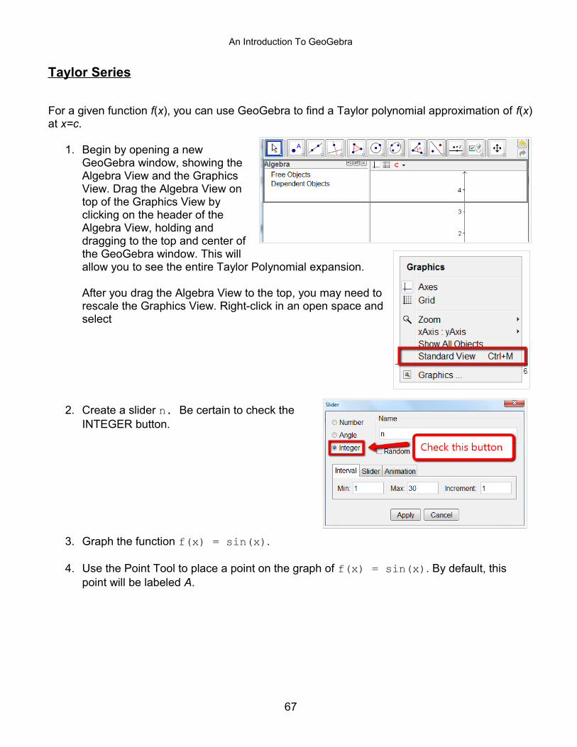
1. Begin by opening a new GeoGebra window, showing the Algebra View and the Graphics View. Drag the Algebra View on top of the Graphics View by clicking on the header of the Algebra View, holding and dragging to the top and center of the GeoGebra window. This will allow you to see the entire Taylor Polynomial expansion.

After you drag the Algebra View to the top, you may need to rescale the Graphics View. Right-click in an open space and select

2. Create a slider n. Be certain to check the INTEGER button.

3. Graph the function f(x) = sin(x).

4. Use the Point Tool to place a point on the graph of f(x) = sin(x). By default, this point will be labeled A.

67


5. Access the Graphics View Properties by Options Menu → Settings... or by right-clicking in an open space in the Graphics View, and selecting Graphics... at the bottom of the context menu. Make the changes shown at right. This will make your coordinate axes “trig-friendly.”

6. You should now have something that looks like the figure at right.

7. In the Input Line, type in the command TaylorPolynomial[ f(x),x(A),n] .

8. Slowly drag the slider.

Things to Try...

• Enhance your sketch by changing colors.• Open the Spreadsheet View and create a table of values for f(x) and for the Taylor

Polynomial.• Export your sketch to a Dynamic Worksheet.

68


Lower Sums, Upper Sums, and Trapezoidal Sums

You will now create a dynamic worksheet that illustrates how lower, upper, and trapezoidal sums can be used to approximate the area between a function and the x-axis, which can be used to introduce the concept of integral to students.

1. Open a new GeoGebra file. Show the Algebra View,and coordinate axes. Set labeling options to New Points Only.

2. Graph the cubic polynomial f(x) = -0.5x3 + 2x2 – x + 1

3. Use the Point Tool to place points A and B on the x-axis. You can also use the command A = Point[ xAxis ] . Points A and B will be the limits of integration.

4. Create a slider n with interval 1 to 50 and increment 1.

5. Enter: uppersum = UpperSum[f, x(A), x(B), n].

6. Enter: lowersum = LowerSum[f, x(A), x(B), n].

7. Enter: trapezoidalsum = TrapezoidalSum[f, x(A), x(B), n]

8. Enter: integral = Integral[f, x(A), x(B)]

9. Create a Dynamic Text Box for each of the sums constructed in steps 5-8.

69


10.Create a checkbox to hide and show each of the four sums created in steps 5-8 as well as the textbox that goes along with it. You should have four checkboxes when done, each controlling one sum and one text box.

When you create your Check Box, just click on the objects you want to be controlled by the check box. I clicked on uppersum in the Algebra View, and I clicked on the Text Box in the Graphics View.

Things to Try...

Arrange the objects on your screen so similar objects are close together and enhance your construction by adding color to the various objects. Consider making everything associated with one particular sum, say, the Upper Sum, all one color.

Export this to a Dynamic Worksheet.

70


Newton's Method

This next construction will demonstrate the power of the Spreadsheet. If the Spreadsheet View is not open, open it. Close the Algebra view if it is open. Change the Labeling options to No New Objects.

1. Start by graphing your favorite cubic function, then adjust the axes (shift-drag on the axis) if need be so you can see the entire function.

2. Place a point on the x-axis by using the Point Tool or by typing Point[xAxis] in the Input Line. Since this is the first point created, it will be known as A.

3. Enter each of the following in the Input Line one at a time, pressing Enter after each:

A1 = A

B1 = PerpendicularLine[ A1, xAxis ]

C1 = Intersect[ f , B1 ]

D1 = Tangent[ C1, f ]

A2 = Intersect[ D1, xAxis ]

4. Select cells B1-D1 and copy them down to B2-D2 by clicking and dragging the small blue box.

5. Select cells A2-D2 and copy them down to cells A10-D10 by clicking and dragging the small blue box.

6. You can enhance your file by changing the colors of a column. Click on the column header, then go to Edit Menu → Object Properties → Color Tab

Things to Try... Change f(x) Export to a Dynamic Worksheet.

71


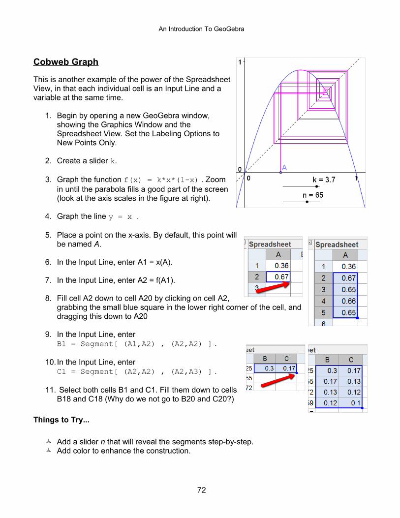
Cobweb Graph

This is another example of the power of the Spreadsheet View, in that each individual cell is an Input Line and a variable at the same time.

1. Begin by opening a new GeoGebra window, showing the Graphics Window and the Spreadsheet View. Set the Labeling Options to New Points Only.

2. Create a slider k.

3. Graph the function f(x) = k*x*(1-x) . Zoom in until the parabola fills a good part of the screen (look at the axis scales in the figure at right).

4. Graph the line y = x .

5. Place a point on the x-axis. By default, this point will be named A.

6. In the Input Line, enter A1 = x(A).

7. In the Input Line, enter A2 = f(A1).

8. Fill cell A2 down to cell A20 by clicking on cell A2, grabbing the small blue square in the lower right corner of the cell, and dragging this down to A20

9. In the Input Line, enter B1 = Segment[ (A1,A2) , (A2,A2) ] .

10. In the Input Line, enter C1 = Segment[ (A2,A2) , (A2,A3) ] .

11. Select both cells B1 and C1. Fill them down to cells B18 and C18 (Why do we not go to B20 and C20?)

Things to Try...

Add a slider n that will reveal the segments step-by-step. Add color to enhance the construction.

72


12. Creating Dynamic WorksheetsWe have already exported our GeoGebra Files to Dynamic Worksheets. This section will show you what the things on the Advanced Tab will do.

We will start with the User Interface, and the Check Boxes available there.

User InterfaceDo you want the Menubar, or Toolbar, or Toolbar help, or Input Bar to show in your applet? If so, you should check the appropriate box.

RULE 1: Show Toolbar and Show Toolbar Help should be checked together.RULE 2: Enable Save, Print & Undo should always be checked whenever Double Click Opens Application Window (FUNCTIONALITY) is checked.

73


Functionality

The first two check boxes are self-explanatory. I rarely check the first one (this will allow the user to change object properties and the like). I usually check the second one (sometimes labels get it the way.

RULE 3: Whenever you create a Random file, you must check Show Icon To Reset Construction. This will allow the user to create a new problem made possible by the RandomBetween command.

RULE 4: Checking Double-click Opens Application Window allows the user to double click on the applet, have it open in a GeoGebra window, and make the file their own. Useful, but be careful using it with students.

RULE 5: I have never used the last box. Try it, though. You may like it.

RULE 6: If you have properly resized your GeoGebra window, you will never need to mess with these numbers.

If you use Moodle, or if you have a class wiki or a blog, the CLIPBOARD: MOODLE will allow you to embed applets in your moodle, blog or wiki page.

Other than that, I typically use FILE: html.

74


13. Customizing the ToolbarCustomizing the Tool Bar is something I found useful in Geometry. For example, I may want my students to construct a parallel line through a given point, but with the Parallel Line Tool available, this is not difficult to do.

Let's make a custom tool bar so students can construct the Perpendicular Bisector of a segment. Begin by opening a new GeoGebra window, and hiding the Algebra View and the Coordinate Axes.

1. Go to Tools Menu → Customize Toolbar. The window on the left shows the tools currently available in the tool bar. What we want to do is to remove some of these tools.

2. The tools are organized in this window the same way they are organized in the tool bar. To open up each group of tools, just click on the small + icon.

75


3. I like to begin by opening up the Move Tool Icon by clicking on the small + next to the Move Tool Icon, then just removing ALL the tools in the category. I do this for each tool. This way, I can select only those tools I want to use.

Of course, this is just me. You may discover a better method that suites you!

4. These are the tools I have included in my Perpendicular Bisector Toolbar.

5. You will need to use the input bar to plot two points and the segment between the two point. For example, I entered A = (1,0), B = (5,2), and Segment[ A , B ] because I had no tools to make these objects.

Things to Try...

Create a Custom Tool Bar for another common construction. Export to a Dynamic Worksheet.

76


14. Useful Links and Information: Your GeoGebra to-do List

1. Remember to visit the GeoGebra Website: http://www.geogebra.org

2. Remember to register on the forum: www.geogebra.org/forum/

3. Remember to visit GeoGebra on Facebook: www.facebook.com/geogebra

4. Remember to work through the tutorials for beginning to advanced users: http://math4allages.wordpress.com/geogebra/

5. Remember to watch the video tutorials on GeoGebra's YouTube Channel: http://www.youtube.com/user/GeoGebraChannel

6. Remember to visit the GeoGebra Wiki: http://www.geogebra.org/en/wiki/index.php/Main_Page

7. Remember to visit GeoGebraTube: http://www.geogebratube.org

77

Documents

An Introduction to GeoGebra - Mathemina/teaching/5270s13/Intro_to_Geogebra.pdfAn Introduction To GeoGebra An Introduction to GeoGebra ... as the Inverse Filling check box. It's ok