An Introduction to Finite Element Analysis - Triton Racingsae.eng.ucsd.edu/wp-content/uploads/Uploaded Forms and Files... · An Introduction to Finite Element Analysis With Emphasis

12/3/2012 ▪ Slide 1

Copyright © 2012 ▪ Luxon Engineering ▪ Proprietary and Confidential ▪ All Rights Reserved.

An Introduction to Finite Element Analysis With Emphasis on Altair HyperWorks Suite Applications for FSAE December 3rd, 2012

Billy Wight President Luxon Engineering

12/3/2012 ▪ Slide 2


What is FEA? Finite Element Analysis is not a black box!

• Too often FEA is regarded as quick to do, or simple, but in reality it is quite complex • Today’s software has made the FEA simple to use which makes it easy to make mistakes

without knowing! • SolidWorks is a great example…

• The analysis results are only as good as the engineer performing the analysis

FEA

12/3/2012 ▪ Slide 3


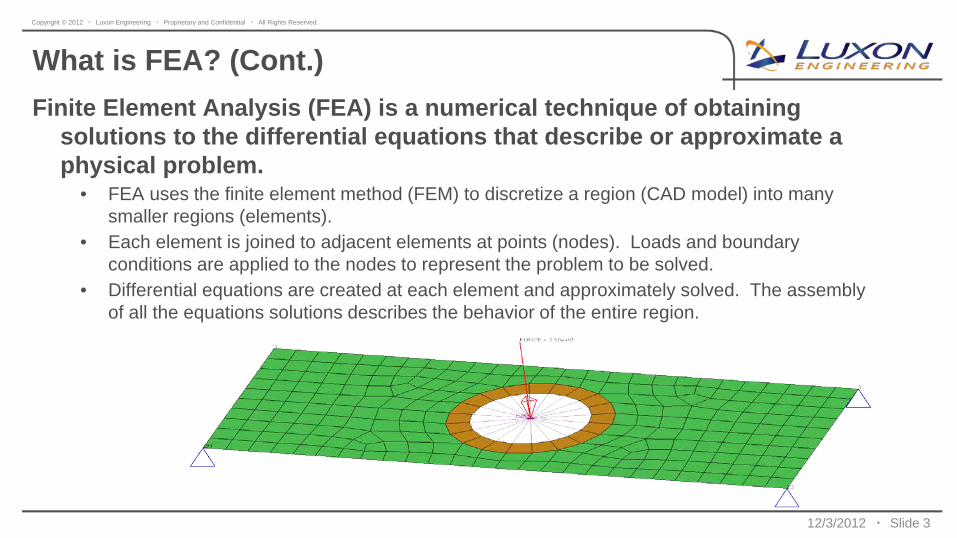
What is FEA? (Cont.) Finite Element Analysis (FEA) is a numerical technique of obtaining

solutions to the differential equations that describe or approximate a physical problem.

• FEA uses the finite element method (FEM) to discretize a region (CAD model) into many smaller regions (elements).

• Each element is joined to adjacent elements at points (nodes). Loads and boundary conditions are applied to the nodes to represent the problem to be solved.

• Differential equations are created at each element and approximately solved. The assembly of all the equations solutions describes the behavior of the entire region.

12/3/2012 ▪ Slide 4


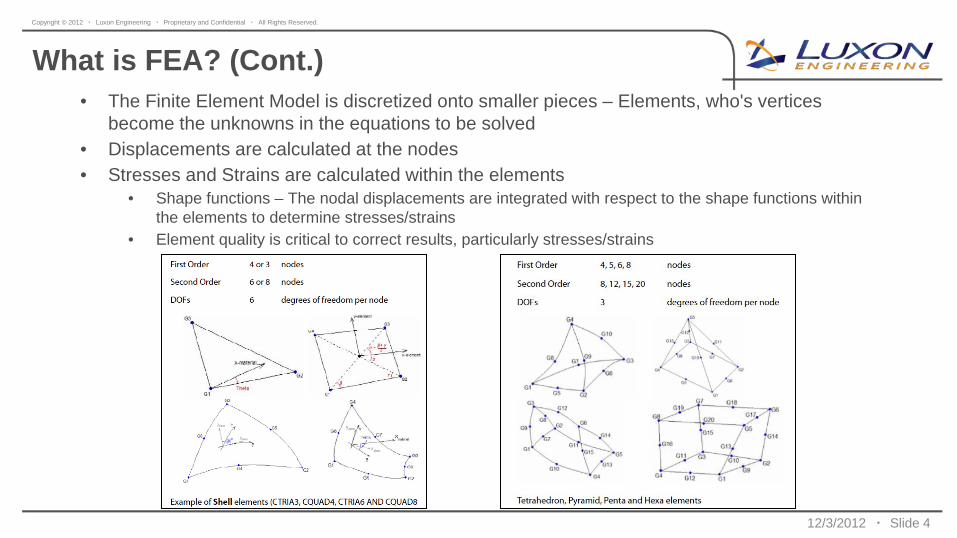
What is FEA? (Cont.) • The Finite Element Model is discretized onto smaller pieces – Elements, who's vertices

become the unknowns in the equations to be solved • Displacements are calculated at the nodes • Stresses and Strains are calculated within the elements

• Shape functions – The nodal displacements are integrated with respect to the shape functions within the elements to determine stresses/strains

• Element quality is critical to correct results, particularly stresses/strains

12/3/2012 ▪ Slide 5


Types of Analysis Many applications of FEA/FEM:

• Structural Linear Static • Structural Quasi-Dynamic and Dynamic • Modal (Frequency) and Buckling • Fatigue • Computational Fluid Dynamics (CFD) • Thermal and Heat Transfer • Electromagnetic (EMS) • Rigid-Body Dynamics

• Dynamic motion solvers, not really FEM, but a fairly typical engineering analysis

• Combinations of the above • Fluid-Structure interactions (CFD+FEA) • Flexible-Body Dynamics (Structural Analysis + Rigid-Body Dynamics) • Others…

• Optimization Studies of any of the above

12/3/2012 ▪ Slide 6


What is Linear Static? The most common type of analysis you will preform

• Linear: • Material linearity - linear elastic, properties do not change with respect to strain, strain rate, etc.

• Most metals, some plastics • Deformations must be linear

• Must have small deformations and small rotations • Most not have snap-through response (buckling)

• Boundary conditions must be constant • No contact • No sliding • No friction

• Static: • Boundary conditions do not change in time

• Loading and constraints are always constant • Loading must be assumed to be applied slowly

• No inertial effects

12/3/2012 ▪ Slide 7


Math (Linear Static)

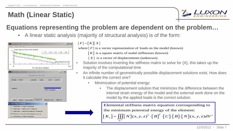
Equations representing the problem are dependent on the problem… • A linear static analysis (majority of structural analysis) is of the form:

• Solution involves inverting the stiffness matrix to solve for {X}, this takes up the majority of the computational time

• An infinite number of geometrically possible displacement solutions exist, How does it calculate the correct one?

• Minimization of potential energy: • The displacement solution that minimizes the difference between the

internal strain energy of the model and the external work done on the model by the applied loads is the correct solution.

{ } [ ]{ }{ }[ ]{ }

where is a vector representation of loads on the model (known)

is a square matrix of nodal stiffnesses (known)

is a vector of displacements (unknown)

F K X

F

K

X

=

[ ] [ ] [ ] [ ] [ ] [ ]

Elemental stiffness matrix equation corrosponding to the minimum potential energy of the element:

( , , ) ( , , )e

TT ee

V

K N x y z B C B N x y z dV= ⋅ ⋅ ⋅ ⋅∫∫∫

12/3/2012 ▪ Slide 8


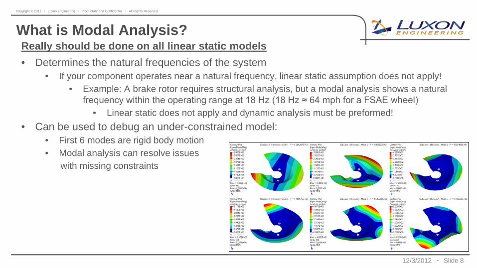
What is Modal Analysis? Really should be done on all linear static models

• Determines the natural frequencies of the system • If your component operates near a natural frequency, linear static assumption does not apply!

• Example: A brake rotor requires structural analysis, but a modal analysis shows a natural frequency within the operating range at 18 Hz (18 Hz ≈ 64 mph for a FSAE wheel)

• Linear static does not apply and dynamic analysis must be preformed! • Can be used to debug an under-constrained model:

• First 6 modes are rigid body motion • Modal analysis can resolve issues with missing constraints

12/3/2012 ▪ Slide 9


Math (Modal) An undamped modal (frequency) analysis is of the form:

[ ]{ } [ ]{ }[ ][ ]{ }{ }

0

where is a matrix representation of the mass and loads on the model (known)

is a square matrix of nodal stiffnesses (known)

is a vector of displacements (unknown)

i

M X K X

M

K

X

X

+ =

{ } { }

{ } { }

[ ]{ } [ ]{ }{ }

2

2

s a vector of accelerations (unknown)

The Solution assumes:sin( )

so that

sin( )

The solution for the naturalfrequency can be written as:

0

where is the mode sha

o

o

th

ii i

thi

X X t

X X t

i

K X M X

X i

ω

ω ω

ω

= ⋅

= − ⋅

− =

pe and is the corrosponding natural frequencyiω

12/3/2012 ▪ Slide 10


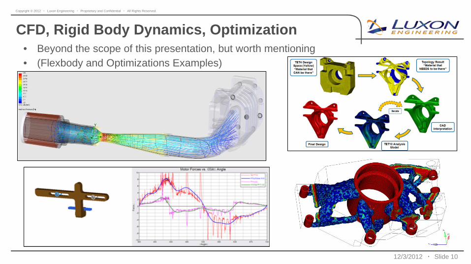
CFD, Rigid Body Dynamics, Optimization • Beyond the scope of this presentation, but worth mentioning • (Flexbody and Optimizations Examples)

12/3/2012 ▪ Slide 11


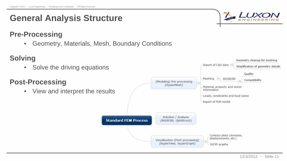
General Analysis Structure

Pre-Processing • Geometry, Materials, Mesh, Boundary Conditions

Solving • Solve the driving equations

Post-Processing • View and interpret the results

12/3/2012 ▪ Slide 12


Pre-Processing: Geometry

Geometry Definition • Used to create the mesh (nodes and elements) • Typically imported from a CAD program

• SolidWorks, Pro/Engineer, Catia, Unigraphics, etc. • Can be created within the analysis software

• Usually a very tedious process

Geometry Cleanup • Unnecessary model details are removed to simplify meshing

• Small holes, fillets and chamfers, shared edge removal, sliver surface removal • Can be done within the FE program or before CAD import

12/3/2012 ▪ Slide 13


Pre-Processing: Material Material Definition

• Various material properties need to be defined • Analysis Dependent…

• Linear Static • Young’s Modulus (E) • Poisson’s Ratio (ν) • Density (ρ)

• Material properties available online: • www.matweb.com

• Physical testing • Most accurate • Unavailable material data

12/3/2012 ▪ Slide 14


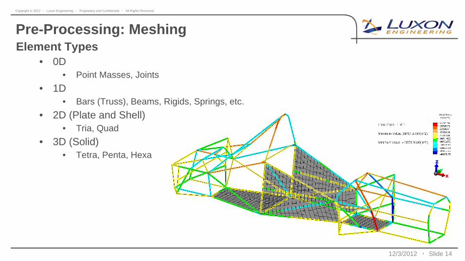
Pre-Processing: Meshing Element Types

• 0D • Point Masses, Joints

• 1D • Bars (Truss), Beams, Rigids, Springs, etc.

• 2D (Plate and Shell) • Tria, Quad

• 3D (Solid) • Tetra, Penta, Hexa

12/3/2012 ▪ Slide 15


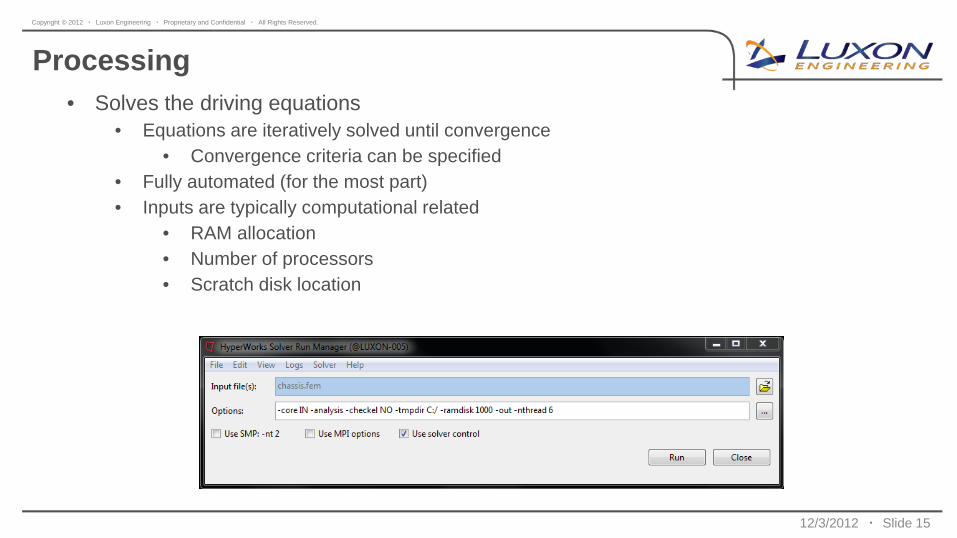
Processing • Solves the driving equations

• Equations are iteratively solved until convergence • Convergence criteria can be specified

• Fully automated (for the most part) • Inputs are typically computational related

• RAM allocation • Number of processors • Scratch disk location

12/3/2012 ▪ Slide 16


Post-Processing • View and interpret the results

• Many plotting options are available • Deformation (nodal displacement), Stress, Strain, etc. • Contour plots, tensor plots, etc. • Iso-clipping, Planar clipping, etc.

• Lots of analysis type specific options • Damage plot (fatigue) • Pathlines (CFD) • Mode Shape (modal)

12/3/2012 ▪ Slide 17


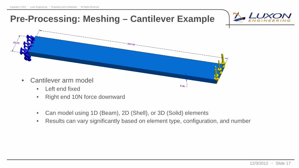
Pre-Processing: Meshing – Cantilever Example

• Cantilever arm model • Left end fixed • Right end 10N force downward

• Can model using 1D (Beam), 2D (Shell), or 3D (Solid) elements • Results can vary significantly based on element type, configuration, and number

12/3/2012 ▪ Slide 18


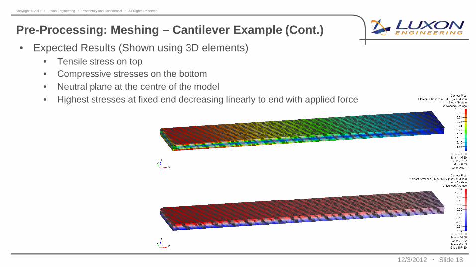
Pre-Processing: Meshing – Cantilever Example (Cont.) • Expected Results (Shown using 3D elements)

• Tensile stress on top • Compressive stresses on the bottom • Neutral plane at the centre of the model • Highest stresses at fixed end decreasing linearly to end with applied force

12/3/2012 ▪ Slide 19


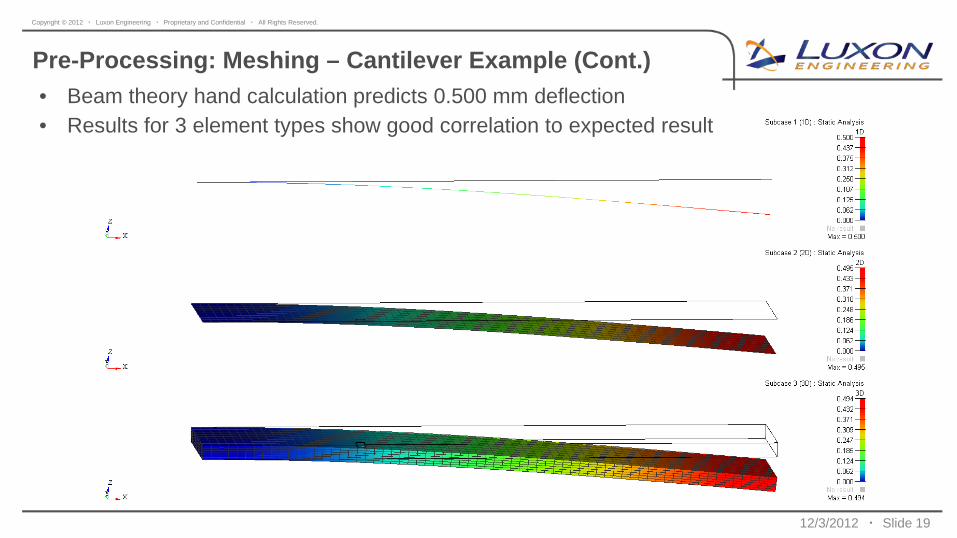
Pre-Processing: Meshing – Cantilever Example (Cont.) • Beam theory hand calculation predicts 0.500 mm deflection • Results for 3 element types show good correlation to expected result

12/3/2012 ▪ Slide 20


Pre-Processing: Meshing – Cantilever Example (Cont.) • Results can vary significantly for different element configurations and densities • It is important to have the correct setup for the analysis you are preforming as it is easy to

get bad results Element Type Order

Element Size Across

Beam

Elements Across

Thickness

Model Total

Elements

Model Total

Nodes

Max Deformation

(mm)

Deformation Error

Stress (MPa), Elements, 58mm In

Elemental Stress Error

Descriptions

Theory - - - - - 0.500 0.0% 13.61 0.0% Beam Theory1D BEAM 1st 3 - 67 158 0.500 0.1% - - Altair 1D Demo (Tensile/Comp Stresses Only)2D QUAD 1st 3 - 536 686 0.495 -0.9% 13.90 2.1% Altair 2D Demo3D HEXA 1st 3 6 3,216 4,304 0.494 -1.1% 11.59 -14.9% Altair 3D Demo2D QUAD 2nd 3 N/A 536 1,833 0.514 2.9% 13.90 2.1% Altair 2D Demo (2nd Order)3D HEXA 2nd 3 6 3,216 16,005 0.509 1.9% 11.59 -14.9% Altair 3D Demo (2nd Order)3D HEXA 1st 1.667 3 5,760 8,228 0.495 -0.9% 9.29 -31.8% Altair 3D Demo3D HEXA 2nd 1.667 3 5,760 30,303 0.508 1.7% 9.28 -31.8% Altair 3D Demo (2nd Order)3D HEXA 1st 0.833 6 43,200 52,297 0.495 -0.9% 11.37 -16.5% Altair 3D Demo Perfect Elements3D HEXA 2nd 0.833 6 43,200 199,813 0.502 0.5% 11.37 -16.5% Altair 3D Demo Perfect Elements (2nd Order)3D HEXA 1st 3 1 536 1,224 0.495 -0.9% 0.22 -98.4% Altair 3D Demo - Bad3D HEXA 2nd 3 1 536 4,130 0.508 1.7% 0.21 -98.4% Altair 3D Demo - Bad (2nd Order)3D TETRA 1st 3 1 3,216 1,224 0.160 -68.0% 4.55 -66.5% Altair 3D Demo - Bad3D TETRA 2nd 3 1 3,216 6,885 0.500 0.1% 6.97 -48.8% Altair 3D Demo - Bad (2nd Order)3D TETRA 1st 1.667 3 34,560 8,228 0.355 -28.9% 10.22 -24.9% Altair 3D Demo - Good3D TETRA 2nd 1.667 3 34,560 55,671 0.506 1.3% 11.67 -14.2% Altair 3D Demo - Good (2nd Order)

3D TETRA 2nd 5.8501 1 1,327 2,572 0.493 -1.3% 7.00 -48.6% SolidWorks Coarse Settings3D TETRA 2nd 2.9251 2 8,190 14,147 0.495 -0.9% 10.30 -24.3% SolidWorks Default Settings3D TETRA 2nd 1.4625 3 58,004 88,969 0.495 -0.9% 12.50 -8.2% SolidWorks Fine Settings3D TETRA 1st 5.8501 1 1,327 443 0.169 -66.2% 5.10 -62.5% SolidWorks Coarse Settings - Draft Quality3D TETRA 1st 2.9251 2 8,190 2,212 0.307 -38.5% 7.50 -44.9% SolidWorks Default Settings - Draft Quality3D TETRA 1st 1.4625 3 58,004 12,598 0.416 -16.7% 12.90 -5.2% SolidWorks Fine Settings - Draft Quality

12/3/2012 ▪ Slide 21


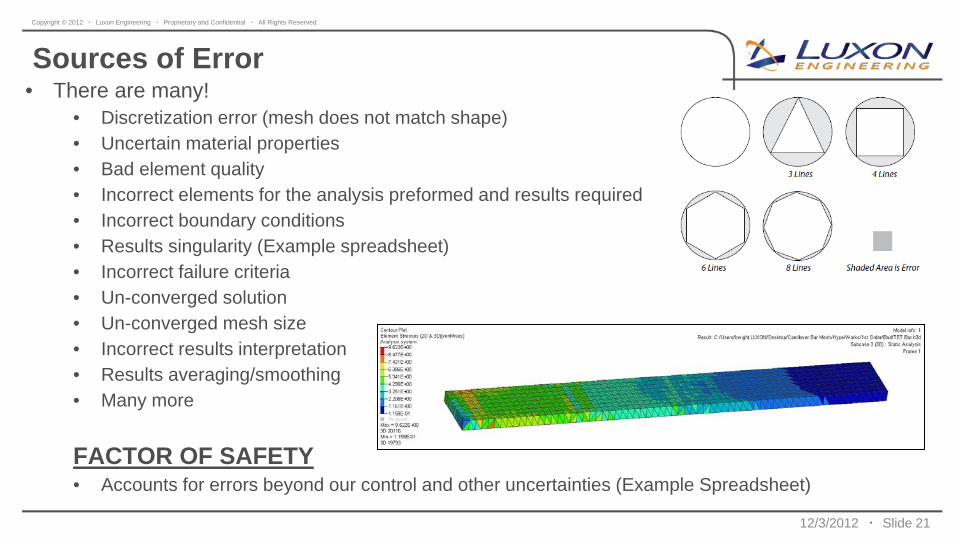
Sources of Error • There are many!

• Discretization error (mesh does not match shape) • Uncertain material properties • Bad element quality • Incorrect elements for the analysis preformed and results required • Incorrect boundary conditions • Results singularity (Example spreadsheet) • Incorrect failure criteria • Un-converged solution • Un-converged mesh size • Incorrect results interpretation • Results averaging/smoothing • Many more

FACTOR OF SAFETY • Accounts for errors beyond our control and other uncertainties (Example Spreadsheet)

12/3/2012 ▪ Slide 22


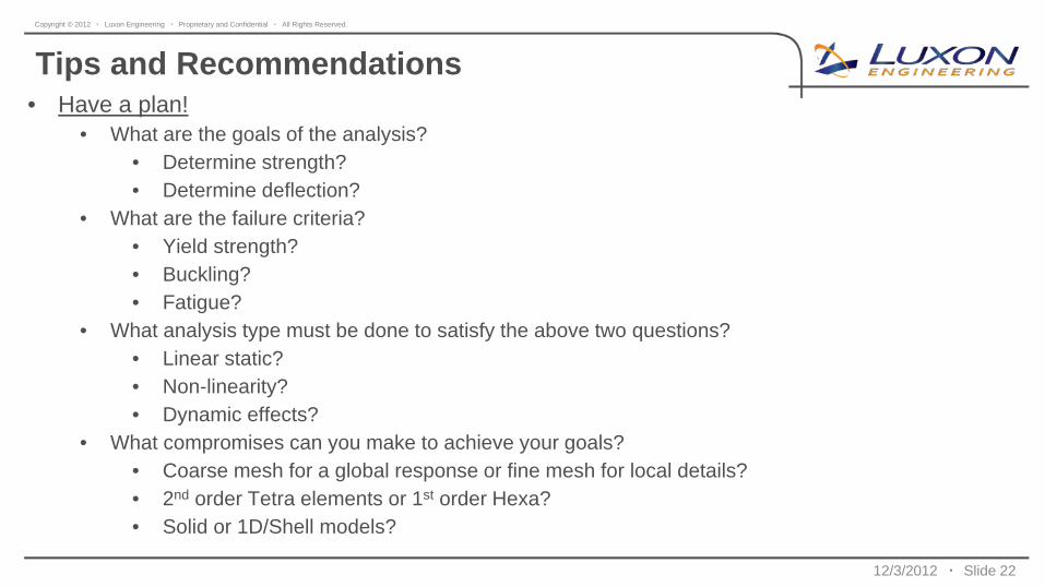
Tips and Recommendations • Have a plan!

• What are the goals of the analysis? • Determine strength? • Determine deflection?

• What are the failure criteria? • Yield strength? • Buckling? • Fatigue?

• What analysis type must be done to satisfy the above two questions? • Linear static? • Non-linearity? • Dynamic effects?

• What compromises can you make to achieve your goals? • Coarse mesh for a global response or fine mesh for local details? • 2nd order Tetra elements or 1st order Hexa? • Solid or 1D/Shell models?

12/3/2012 ▪ Slide 23


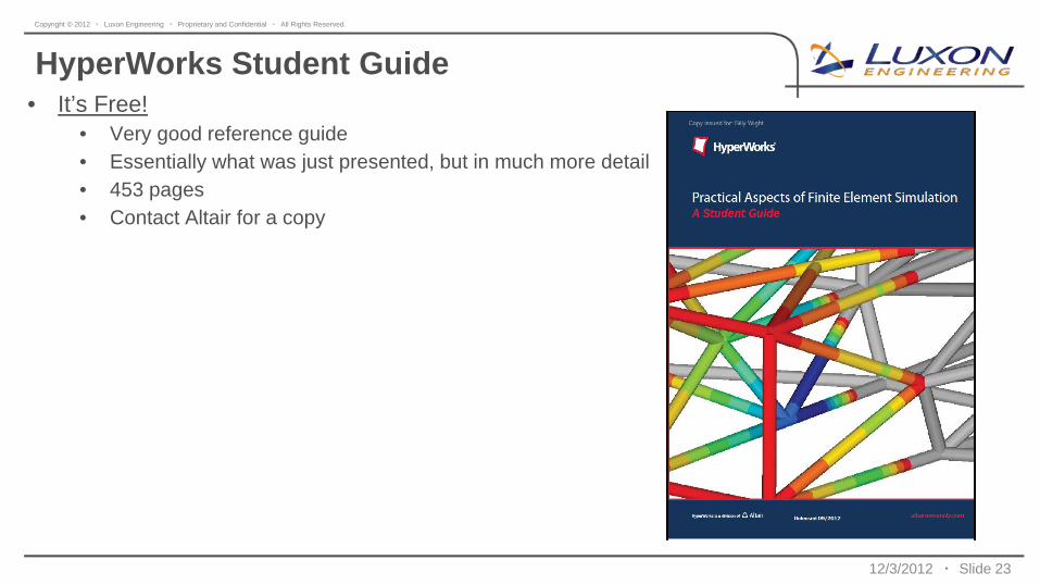
HyperWorks Student Guide • It’s Free!

• Very good reference guide • Essentially what was just presented, but in much more detail • 453 pages • Contact Altair for a copy

12/3/2012 ▪ Slide 24


Linear Static Example • Motocross Suspension Linkage Component

Documents

An Introduction to Finite Element Analysis - Triton Racingsae.eng.ucsd.edu/wp-content/uploads/Uploaded Forms and Files... · An Introduction to Finite Element Analysis With Emphasis