An Introduction to Active Shape Models ∗

Tim Cootes

1 Introduction

Biomedical images usually contain complex objects, which will vary in appear-ance significantly from one image to another. Attempting to measure or detectthe presence of particular structures in such images can be a daunting task.The inherent variability will thwart naive schemes. However, by using modelswhich can cope with the variability it is possible to successfully analyse compleximages.

Here we will consider a number of methods where the model represents theexpected shape and local grey-level structure of a target object in an image.

Model-based methods make use of a prior model of what is expected in theimage, and typically attempt to find the best match of the model to the datain a new image. Having matched the model, one can then make measurementsor test whether the target is actually present.

This approach is a ‘top-down’ strategy, and differs significantly from ‘bottom-up’ methods. In the latter the image data is examined at a low level, lookingfor local structures such as edges or regions, which are assembled into groups inan attempt to identify objects of interest. Without a global model of what toexpect, this approach is difficult and prone to failure.

A wide variety of model based approaches have been explored (see the reviewbelow). This chapter will concentrate on a statistical approach, in which a modelis built from analysing the appearance of a set of labelled examples. Wherestructures vary in shape or texture, it is possible to learn what are plausiblevariations and what are not. A new image can be interpreted by finding thebest plausible match of the model to the image data. The advantages of such amethod are that

• It is widely applicable. The same algorithm can be applied to many dif-ferent problems, merely by presenting different training examples.

• Expert knowledge can be captured in the system in the annotation of thetraining examples.

∗appears as Chapter 7: ”Model-Based Methods in Analysis of Biomedical Images” in”Image Processing and Analysis”, Ed.R.Baldock and J.Graham,Oxford University Press, 2000,pp223-248.

1

• The models give a compact representation of allowable variation, but arespecific enough not to allow arbitrary variation different from that seen inthe training set.

• The system need make few prior assumptions about the nature of theobjects being modelled, other than what it learns from the training set.(For instance, there are no boundary smoothness parameters to be set.)

The models described below require a user to be able to mark ‘landmark’points on each of a set of training images in such a way that each landmarkrepresents a distinguishable point present on every example image. For in-stance, when building a model of the appearance of an eye in a face image,good landmarks would be the corners of the eye, as these would be easy to iden-tify and mark in each image. This constrains the sorts of applications to whichthe method can be applied - it requires that the topology of the object cannotchange and that the object is not so amorphous that no distinct landmarks canbe applied. Unfortunately this makes the method unsuitable in its current formfor objects which exhibit large changes in shape, such as some types of cells orsimple organisms.

The remainder of this chapter will briefly review other model based methods,describe how one form of statistical model can be built and tested, and how suchmodels can be used to interpret objects in new images.

2 Background

The simplest model is to use a typical example as a ‘golden image’. A correlationmethod can be used to match (or register) the golden image to a new image.If structures in the golden image have been labelled, this match then gives theapproximate position of the structures in the new image. For instance, onecan determine the approximate locations of many structures in an MagneticResonance (MR) image of a brain by registering a standard image, where thestandard image has been suitably annotated by human experts. However, thevariability of both shape and texture of most targets limits the precision of thismethod.

One approach to representing the variations observed in an image is to ‘hand-craft’ a model to solve the particular problem currently addressed. For instanceYuille et al [23] build up a model of a human eye using combinations of param-eterised circles and arcs. Though this can be effective it is complicated, and acompletely new solution is required for every application.

Staib and Duncan [22] represent the shapes of objects in medical imagesusing fourier descriptors of closed curves. The choice of coefficients affects thecurve complexity. Placing limits on each coefficient constrains the shape some-what but not in a systematic way. It can be shown that such fourier models canbe made directly equivalent to the statistical models described below, but arenot as general. For instance, they cannot easily represent open boundaries.

2

Kass et al [15] introduced Active Contour Models (or ‘snakes’) which areenergy minimising curves. In the original formulation the energy has an internalterm which aims to impose smoothness on the curve, and an external termwhich encourages movement toward image features. They are particularly usefulfor locating the outline of general amorphous objects, such as some cells (seeChapter 3, secion 3.1 for the application of a snake to microscope images).However, since no model (other than smoothness) is imposed, they are notoptimal for locating objects which have a known shape. As the constraints areweak, this can easily converge to incorrect solutions.

Alternative statistical approaches are described by Grenander et al [10] andMardia et al [18]. These are, however, difficult to use in automated imageinterpretation. Goodall [9] and Bookstein [2] use statistical techniques for mor-phometric analysis, but do not address the problem of automated interpretation.Kirby and Sirovich [16] describe statistical modelling of grey-level appearance(particularly for face images) but do not address shape variability.

A more comprehensive survey of deformable models used in medical imageanalysis is given in [19].

3 Application

We demonstrate the method by applying it to two problems, that of locatingfeatures in images of the human face and that of locating the cartilage in MRimages of a knee.

Images of the face can demonstrate a wide degree of variation in both shapeand texture. Appearance variations are caused by differences between individ-uals, the deformation of an individual face due to changes in expression andspeaking, and variations in the lighting. Typically one would like to locate thefeatures of a face in order to perform further processing (see Figure 1). Theultimate aim may vary widey, from determining the identity or expression ofthe person to deciding in which direction they are looking [17].

When analysing the MR images of the knee (Figure 2), we wish to accuratelylocate the boundary of the cartilage in order to estimate its thickness and volume[21].

In both applications difficulties arise because of the complexity of the targetimages. Bottom-up approaches are unlikely to solve the problems successfully.Complex images give rise to many primitives, which must be linked togethercorrectly to give a successful interpretation. The number of ways in whichthey can be connected explodes exponentially with the number of components.Thus a bottom-up approach can become inefficient for complex scenes. Bybuilding models from sets of examples we can apply the same algorithms toboth applications. In each case the output is a set of model landmark pointswhich best match the image data, together with the model parameters requiredto generate the points. The points or the parameters can then be used infurther processing. For instance, in the face example the parameters can beused to estimate the person’s expression or identity. In the knee example, we

3

Figure 1: Example face image annotated with landmarks

Figure 2: Example MR image of knee with cartilage outlined

4

can estimate the area of the cross-section of the cartilage from the points.

4 Theoretical Background

Here we describe the statistical models of shape and appearance used to repre-sent objects in images. A model is trained from a set of images annotated bya human expert. By analysing the variations in shape and appearance over thetraining set, a model is built which can mimic this variation. To interpret a newimage we must find the parameters which best match a model instance to theimage. We describe an algorithm which can do this efficiently. Having fit themodel to the image, the parameters or the model point positions can be usedto classify or make measurements, or as an input to further processing.

4.1 Building Models

In order to locate a structure of interest, we must first build a model of it. Tobuild a statistical model of appearance we require a set of annotated imagesof typical examples. We must first decide upon a suitable set of landmarkswhich describe the shape of the target and which can be found reliably on everytraining image.

4.1.1 Suitable Landmarks

Good choices for landmarks are points at clear corners of object boundaries, ‘T’junctions between boundaries or easily located biological landmarks. However,there are rarely enough of such points to give more than a sparse desription of theshape of the target object. We augment this list with points along boundarieswhich are arranged to be equally spaced between well defined landmark points(Figure 3).

Object Boundary

High Curvature

‘T’ Junction

Equally spacedintermediate points

Figure 3: Good landmarks are points of high curvature or junctions. Interme-diate points can be used to define boundary more precisely.

To represent the shape we must also record the connectivity defining howthe landmarks are joined to form the boundaries in the image. This allowsus to determine the direction of the boundary at a given point. Suppose thelandmarks along a curve are labelled {(x1, y1), (x2, y2), . . . , (xn, yn)}.

5

For a 2-D image we can represent the n landmark points, {(xi, yi)}, for asingle example as the 2n element vector, x, where

x = (x1, . . . , xn, y1, . . . , yn)T (1)

If we have s training examples, we generate s such vectors xj . Before wecan perform statistical analysis on these vectors it is important that the shapesrepresented are in the same co-ordinate frame. The shape of an object is nor-mally considered to be independent of the position, orientation and scale of thatobject. A square, when rotated, scaled and translated, remains a square.

Appendix 6 describes how to align a set of training shapes into a commonco-ordinate frame. The approach is to translate, rotate and scale each shapeso that the sum of distances of each shape to the mean (D =

∑

|xi − x|2) isminimised.

4.1.2 Statistical Models of Shape

Suppose now we have s sets of points xi which are aligned into a common co-ordinate frame. These vectors form a distribution in the 2n dimensional spacein which they live. If we can model this distribution, we can generate newexamples, similar to those in the original training set, and we can examine newshapes to decide whether they are plausible examples.

To simplify the problem, we first wish to reduce the dimensionality of thedata from 2n to something more manageable. An effective approach is to applyPrincipal Component Analysis (PCA) to the data. The data form a cloud ofpoints in the 2n-D space, though by aligning the points they lie in a (2n− 4)-Dmanifold in this space. PCA computes the main axes of this cloud, allowingone to approximate any of the original points using a model with less than 2nparameters (See Appendix 6).

If we apply a PCA to the data, we can then approximate any of the trainingset, x using

x ≈ x + Pb (2)

where P = (p1|p2| . . . |pt) contains t eigenvectors of the covariance matrixand b is a t dimensional vector given by

b = PT (x − x) (3)

(See Appendix 6 for details).The vector b defines a set of parameters of a deformable model. By varying

the elements of b we can vary the shape, x using Equation 2. The variance ofthe ith parameter, bi, across the training set is given by λi. By applying limitsof ±3

√λi to the parameter bi we ensure that the shape generated is similar to

those in the original training set.We usually call the model variation corresponding to the ith parameter, bi,

as the ith mode of the model. The eigenvectors, P, define a rotated co-ordinate

6

frame, aligned with the cloud of original shape vectors. The vector b definespoints in this rotated frame.

4.1.3 Examples of Shape Models

Figure 4 shows example shapes from a training set of 300 labelled faces (see Fig-ure 1 for an example image showing the landmarks). Each image is annotatedwith 133 landmarks. The shape model has 36 parameters, and can explain 98%of the variance in the landmark positions in the training set. Figure 5 shows theeffect of varying the first three shape parameters in turn between ±3 standarddeviations from the mean value, leaving all other parameters at zero. These‘modes’ explain global variation due to 3D pose changes, which cause move-ment of all the landmark points relative to one another. Less significant modescause smaller, more local changes. The modes obtained are often similar tothose a human would choose if designing a parameterised model, for instanceshaking and nodding the head, or changing expression. However, they are de-rived directly from the statistics of a training set and will not always separateshape variation in an obvious manner.

Figure 4: Example shapes from training set of faces

Figure 6 shows examples from a training set of 33 knee cartilage boundaries.(See Figure 2 for an example of the corresponding images). Each is annotatedwith 42 landmarks. When we apply the alignment and PCA as described above,we generate a model with 15 modes. Figure 7 shows the effect of varying thefirst three shape parameters in turn between ±3 standard deviations from themean value, leaving all other parameters at zero.

Thus in the case of faces the use of the PCA reduced the dimension of theshape vectors from 266 to 36. In the case of the knees, the dimension went from84 to 15.

4.1.4 Fitting a Model to New Points

A particular value of the shape vector, b, corresponds to a point in the rotatedspace described by P. It therefore corresponds to an example model. This can

7

Mode 1

Mode 2

Mode 3

Figure 5: Effect of varying each of first three face model shape parameters inturn between ±3 s.d.

Figure 6: Example shapes from training set of knee cartilages

Mode 1

Mode 2

Mode 3

Figure 7: Effect of varying each of first three cartilage model shape parametersin turn between ±3 s.d.

8

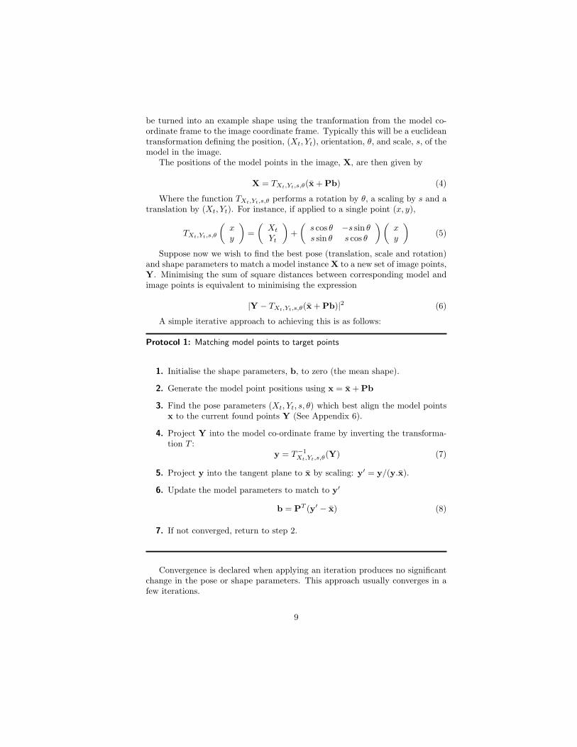
be turned into an example shape using the tranformation from the model co-ordinate frame to the image coordinate frame. Typically this will be a euclideantransformation defining the position, (Xt, Yt), orientation, θ, and scale, s, of themodel in the image.

The positions of the model points in the image, X, are then given by

X = TXt,Yt,s,θ(x + Pb) (4)

Where the function TXt,Yt,s,θ performs a rotation by θ, a scaling by s and atranslation by (Xt, Yt). For instance, if applied to a single point (x, y),

TXt,Yt,s,θ

(

xy

)

=

(

Xt

Yt

)

+

(

s cos θ −s sin θs sin θ s cos θ

)(

xy

)

(5)

Suppose now we wish to find the best pose (translation, scale and rotation)and shape parameters to match a model instance X to a new set of image points,Y. Minimising the sum of square distances between corresponding model andimage points is equivalent to minimising the expression

|Y − TXt,Yt,s,θ(x + Pb)|2 (6)

A simple iterative approach to achieving this is as follows:

Protocol 1: Matching model points to target points

1. Initialise the shape parameters, b, to zero (the mean shape).

2. Generate the model point positions using x = x + Pb

3. Find the pose parameters (Xt, Yt, s, θ) which best align the model pointsx to the current found points Y (See Appendix 6).

4. Project Y into the model co-ordinate frame by inverting the transforma-tion T :

y = T−1Xt,Yt,s,θ(Y) (7)

5. Project y into the tangent plane to x by scaling: y′ = y/(y.x).

6. Update the model parameters to match to y′

b = PT (y′ − x) (8)

7. If not converged, return to step 2.

Convergence is declared when applying an iteration produces no significantchange in the pose or shape parameters. This approach usually converges in afew iterations.

9

4.1.5 Testing How Well the Model Generalises

The shape models described use linear combinations of the shapes seen in atraining set. In order to be able to generate new versions of the shape to matchto image data, the training set must exhibit all the variation expected in theclass of shapes being modelled. If it does not, the model will be over-constrainedand will not be able to match to some types of new example. For instance, amodel trained only on squares will not generalise to rectangles.

One approach to estimating how well the model will perform is to use ‘leave-one-out’ experiments (see Chapter 4). Given a training set of s examples, builda model from all but one, then fit the model to the example missed out andrecord the error (for instance using (6)). Repeat this, missing out each of thes examples in turn. If the error is unacceptably large for any example, moretraining examples are probably required. However, small errors for all examplesonly mean that there is more than one example for each type of shape variation,not that all types are properly covered (though it is an encouraging sign).

Equation (6) gives the sum of square errors over all points, and may averageout large errors on one or two individual points. It is often wise to calculatethe error for each point and ensure that the maximum error on any point issufficiently small.

4.1.6 Choice of Number of Modes

Section 4.1.2 suggested that during training the number of modes, t, could bechosen so as to explain a given proportion (eg 98%) of the variance exhibited inthe training set.

An alternative approach is to choose enough modes that the model canapproximate any training example to within a given accuracy. For instance, wemay wish that the best approximation to an example has every point withinone pixel of the corresponding example points.

To achieve this we build models with increasing numbers of modes, testingthe ability of each to represent the training set. We choose the first model whichpasses our desired criteria.

Additional confidence can be obtained by performing this test in a miss-one-out manner. We choose the smallest t for the full model such that modelsbuilt with t modes from all but any one example can approximate the missingexample sufficiently well.

4.2 Image Interpretation with Models

4.2.1 Overview

To interpret an image using a model, we must find the set of parameters whichbest match the model to the image. This set of parameters defines the shape andposition of the target object in an image, and can be used for further processing,such as to make measurements or to classify the object.

10

There are several approaches which could be taken to matching a modelinstance to an image, but all can be thought of as optimising a cost function.For a set of model parameters, c, we can generate an instance of the modelprojected into the image. We can compare this hypothesis with the targetimage, to get a fit function F (c). The best set of parameters to interpret theobject in the image is then the set which optimises this measure. For instance,if F (c) is an error measure, which tends to zero for a perfect match, we wouldlike to choose parameters, c, which minimise the error measure.

Thus, in theory all we have to do is to choose a suitable fit function, and usea general purpose optimiser to find the minimum. There are many approachesto optimisation which can be used, for instance simplex, Powells Method [20] orGenetic Algorithms [8]. The minimum is defined only by the choice of function,the model and the image, and is independent of which optimisation method isused to find it. However, in practice, care must be taken to choose a functionwhich can be optimised rapidly and robustly, and an optimisation method tomatch.

4.2.2 Choice of Fit Function

Ideally we would like to choose a fit function which represents the probabilitythat the model parameters describe the target image object, P (c|I) (where Irepresents the image). We then choose the parameters which maximise thisprobability.

In the case of the shape models described above, the parameters we can varyare the shape parameters, b, and the pose parameters Xt, Yt, s, θ.

The form of the fit measure, however, is harder to determine. If we assumethat the shape model represents boundaries and strong edges of the object, auseful measure is the distance between a given model point and the neareststrong edge in the image (Figure 8).

on Normal (X’,Y’)

Model Boundary

Image Object

Nearest Edge

Model Point (X,Y)

Normal to ModelBoundary

Figure 8: An error measure can be derived from the distance between modelpoints and strongest nearby edges.

If the model point positions are given in the vector X, and the nearest edge

11

points to each model point are X′, then an error measure is

F (b,Xt, Yt, s, θ) = |X′ − X|2 (9)

Alternatively, rather than looking for the best nearby edges, one can searchfor structure nearby which is most similar to that occuring at the given modelpoint in the training images (see below).

It should be noted that this fit measure relies upon the target points, X′,begin the correct points. If some are incorrect, due to clutter or failure of theedge/feature detectors, Equation (9) will not be a true measure of the qualityof fit.

An alternative approach is to sample the image around the current modelpoints, and determine how well the image samples match models derived fromthe training set. This approach was taken by Haslam et al [11].

A related approach is to model the full appearance of the object, includingthe internal texture. The quality of fit of such an appearance model can beassessed by measuring the difference between the target image and a syntheticimage generated from the model. This is beyond the scope of this chapter, butis described in detail in [4].

4.2.3 Optimising the Model Fit

Given no initial knowledge of where the target object lies in an image, findingthe parameters which optimise the fit is a difficult general optimisation problem.This can be tackled with general global optimisation techniques, such as GeneticAlgorithms or Simulated Annealing [12].

If, however, we have an initial approximation to the correct solution (weknow roughly where the target object is in an image, due to prior processing),we can use local optimisation techniques such as Powell’s method or Simplex.A good overview of practical numeric optimisation is given by Press et al [20].

However, we can take advantage of the form of the fit function to locate theoptimum rapidly. We derive an algorithm which amounts to a directed searchof the parameter space - the Active Shape Model.

4.3 Active Shape Models

Given a rough starting approximation, an instance of a model can be fit to animage. By choosing a set of shape parameters, b for the model we define theshape of the object in an object-centred co-ordinate frame. We can create aninstance X of the model in the image frame by defining the position, orientationand scale, using Equation 4.

An iterative approach to improving the fit of the instance, X, to an imageproceeds as follows:

Protocol 2: Active Shape Model Algorithm

12

1. Examine a region of the image around each point Xi to find the bestnearby match for the point X′

i

2. Update the parameters (Xt, Yt, s, θ,b) to best fit the new found points X

3. Apply constraints to the parameters, b, to ensure plausible shapes (eglimit so |bi| < 3

√λi).

4. Repeat until convergence.

In practise we look along profiles normal to the model boundary througheach model point (Figure 9). If we expect the model boundary to correspondto an edge, we can simply locate the strongest edge (including orientation ifknown) along the profile. The position of this gives the new suggested locationfor the model point.

Inte

nsity

Distance along profile

Image Structure

Model Point

Profile Normalto Boundary

Model Boundary

Figure 9: At each model point sample along a profile normal to the boundary

However, model points are not always placed on the strongest edge in thelocality - they may represent a weaker secondary edge or some other imagestructure. The best approach is to learn from the training set what to look forin the target image. This is done by sampling along the profile normal to theboundary in the training set, and building a statistical model of the grey-levelstructure.

Suppose for a given point we sample along a profile k pixels either side ofthe model point in the ith training image. We have 2k+1 samples which can beput in a vector gi. To reduce the effects of global intensity changes we samplethe derivative along the profile, rather than the absolute grey-level values. Wethen normalise the sample by dividing through by the sum of absolute elementvalues,

gi →1

∑

j |gij |gi (10)

We repeat this for each training image, to get a set of normalised samples{gi} for the given model point. We assume that these are distributed as a

13

multivariate gaussian, and estimate their mean g and covariance Sg. This givesa statistical model for the grey-level profile about the point. This is repeatedfor every model point, giving one grey-level model for each point.

The quality of fit of a new sample, gs, to the model is given by

f(gs) = (gs − g)T S−1g (gs − g) (11)

This is the Mahalanobis distance of the sample from the model mean, andis linearly related to the log of the probability that gs is drawn from the distri-bution. Minimising f(gs) is equivalent to maximising the probability that gs

comes from the distribution.During search we sample a profile m pixels either side of the current point (

m > k ). We then test the quality of fit of the corresponding grey-level modelat each of the 2(m− k) + 1 possible positions along the sample (Figure 10) andchoose the one which gives the best match (lowest value of f(gs)).

Model

Sampled Profile

Cost of Fit

Figure 10: Search along sampled profile to find best fit of grey-level model

This is repeated for every model point, giving a suggested new position foreach point. We then apply one iteration of the algorithm given in (4.1.4) toupdate the current pose and shape parameters to best match the model to thenew points.

4.3.1 Multi-Resolution Active Shape Models

To improve the efficiency and robustness of the algorithm, it is implementededin a multi-resolution framework. This involves first searching for the object ina coarse image, then refining the location in a series of finer resolution images.This leads to a faster algorithm, and one which is less likely to get stuck on thewrong image structure.

For each training and test image, a gaussian image pyramid is built [3]. Thebase image (level 0) is the original image. The next image (level 1) is formed

14

by smoothing the original then subsampling to obtain an image with half thenumber of pixels in each dimension. Subsequent levels are formed by furthersmoothing and sub-sampling (Figure 11).

Level 1

Level 2

Level 0

Figure 11: A gaussian image pyramid is formed by repeated smoothing andsub-sampling

During training we build statistical models of the grey-levels along normalprofiles through each point, at each level of the gaussian pyramid. We usuallyuse the same number of pixels in each profile model, regardless of level. Since thepixels at level L are 2L times the size of those of the original image, the modelsat the coarser levels represent more of the image (Figure 12). Similarly, duringsearch we need only search a few pixels, (ns), either side of the current pointposition at each level. At coarse levels this will allow quite large movements,and the model should converge to a good solution. At the finer resolution weneed only modify this solution by small amounts.

Level 0

Level 1

Level 2

Figure 12: Statistical models of grey-level profiles represent the same numberof pixels at each level

When searching at a given resolution level, we need a method of determiningwhen to change to a finer resolution, or to stop the search. This is done byrecording the number of times that the best found pixel along a search profileis within the central 50% of the profile (ie the best point is within ns/2 pixels

15

of the current point). When a sufficient number (eg ≥ 90%) of the points areso found, the algorithm is declared to have converged at that resolution. Thecurrent model is projected into the next image and run to convergence again.When convergence is reached on the finest resolution, the search is stopped.

To summarise, the full MRASM search algorithm is as follows:

Protocol 3: Multi-Resolution Search Algorithm

1. Set L = Lmax

2. While L ≥ 0

(a) Compute model point positions in image at level L.

(b) Search at ns points on profile either side each current point

(c) Update pose and shape parameters to fit model to new points

(d) Return to (2a) unless more than pclose of the points are found closeto the current position, or Nmax iterations have been applied at thisresolution.

(e) If L > 0 then L → (L − 1)

3. Final result is given by the parameters after convergence at level 0.

The model building process only requires the choice of three parameters:

Model Parameters

n Number of model pointst Number of modes to usek Number of pixels either side of point to represent in grey-model

The number of points is dependent on the complexity of the object, andthe accuracy with which one wishes to represent any boundaries. The numberof modes should be chosen that a sufficient amount of object variation can becaptured (see 4.1.5 above). The number of pixels to represent in each localgrey model will depend on the width of the boundary structure (however, usingbetween 3 and 7 pixels either side has given good results for many applications).

The search algorithm has four parameters:

Search Parameters (Suggested default)Lmax Coarsest level of gaussian pyramid to searchns Number of sample points either side of current point (2)Nmax Maximum number of iterations allowed at each level (5)pclose Desired proportion of points found within ns/2 of current position (0.9)

16

The levels of the gaussian pyramid to seach will depend on the size of theobject in the image.

4.3.2 Examples of Search

Figure 13 demonstrates using the ASM to locate the features of a face. Themodel instance is placed near the centre of the image and a coarse to fine searchperformed. The search starts at level 3 (1/8 the resolution in x and y comparedto the original image). Large movements are made in the first few iterations,getting the position and scale roughly correct. As the search progresses to finerresolutions more subtle adjustments are made. The final convergence (after atotal of 18 iterations) gives a good match to the target image. In this case atmost 5 iterations were allowed at each resolution, and the algorithm convergesin much less than a second (on a 200MHz PC).

Initial After 2 iterations

After 6 iterations After 18 iterations

Figure 13: Search using Active Shape Model of a face

Figure 14 demonstrates how the ASM can fail if the starting position is toofar from the target. Since it is only searching along profiles around the current

17

position, it cannot correct for large displacements from the correct position. Itwill either diverge to infinity, or converge to an incorrect solution, doing its bestto match the local image data. In the case shown it has been able to locate halfthe face, but the other side is too far away.

Initial After 2 iterations After 20 Iterations

Figure 14: Search using Active Shape Model of a face, given a poor startingpoint. The ASM is a local method, and may fail to locate an acceptable resultif initialised too far from the target

Figure 15 demonstrates using the ASM of the cartilage to locate the structurein a new image. In this case the search starts at level 2, samples at 2 pointseither side of the current point and allows at most 5 iterations per level. Adetailed description of the application of such a model is given by Solloway et.al. in [21].

5 Discussion

Active Shape Models allow rapid location of the boundary of objects with similarshapes to those in a training set, assuming we know roughly where the objectis in the image. They are particularly useful for:

• Objects with well defined shape (eg bones, organs, faces etc)

• Cases where we wish to classify objects by shape/appearance

• Cases where a representative set of examples is available

• Cases where we have a good guess as to where the target is in the image

However, they are not necessarily appropriate for

• Objects with widely varying shapes (eg amorphous things, trees, longwiggly worms etc)

• Problems involving counting large numbers of small things

18

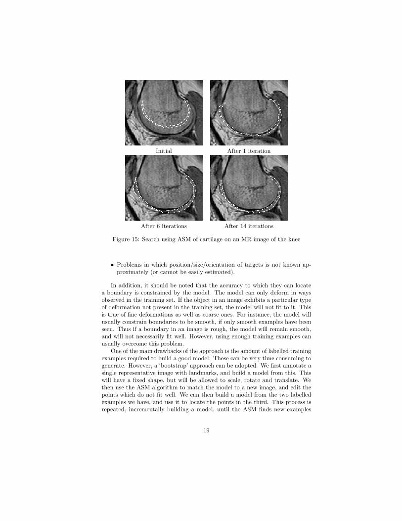
Initial After 1 iteration

After 6 iterations After 14 iterations

Figure 15: Search using ASM of cartilage on an MR image of the knee

• Problems in which position/size/orientation of targets is not known ap-proximately (or cannot be easily estimated).

In addition, it should be noted that the accuracy to which they can locatea boundary is constrained by the model. The model can only deform in waysobserved in the training set. If the object in an image exhibits a particular typeof deformation not present in the training set, the model will not fit to it. Thisis true of fine deformations as well as coarse ones. For instance, the model willusually constrain boundaries to be smooth, if only smooth examples have beenseen. Thus if a boundary in an image is rough, the model will remain smooth,and will not necessarily fit well. However, using enough training examples canusually overcome this problem.

One of the main drawbacks of the approach is the amount of labelled trainingexamples required to build a good model. These can be very time consuming togenerate. However, a ‘bootstrap’ approach can be adopted. We first annotate asingle representative image with landmarks, and build a model from this. Thiswill have a fixed shape, but will be allowed to scale, rotate and translate. Wethen use the ASM algorithm to match the model to a new image, and edit thepoints which do not fit well. We can then build a model from the two labelledexamples we have, and use it to locate the points in the third. This process isrepeated, incrementally building a model, until the ASM finds new examples

19

sufficiently accurately every time, so needs no more training.Both the shape models and the search algorithms can be extended to 3D. The

landmark points become 3D points, the shape vectors become 3n dimensionalfor n points. Although the statistical machinery is identical, a 3D alignmentalgorithm must be used (see [13]). Of course, annotating 3D images with land-marks is difficult, and more points are required than for a 2D object. In addition,the definition of surfaces and 3D topology is more complex than that requiredfor 2D boundaries. However, 3D models which represent shape deformation canbe successfully used to locate structures in 3D datasets such as MR images (forinstance [14]).

The ASM is well suited to tracking objects through image sequences. In thesimplest form the full ASM search can be applied to the first image to locate thetarget. Assuming the object does not move by large amounts between frames,the shape for one frame can be used as the starting point for the search in thenext, and only a few iterations will be required to lock on. More advancedtechniques would involve applying a Kalman filter to predict the motion [1][7].

The shape models described above assume a simple gaussian model for thedistribution of the shape parameters, b. A more general approach is to use amixture of gaussians. We need to ensure that the model generates plausibleshapes. Using a single gaussian we can simply constrain the parameters with abounding box or hyper-ellipse. With a mixture of gaussians we must arrangethat the probability density for the current set of parameters is above a suitablethreshold. Where it isn’t, we can use gradient ascent to find the nearest pointin parameter space which does give a plausible shape [5]. However, in practice,unless large non-gaussian shape variations are observed and the target imagesare noisy or cluttered, using a single gaussian approximation works perfectlywell.

To summarise, by training statistical models of shape from sets of labelledexamples we can represent both the mean shape of a class of objects and thecommon modes of shape variation. To locate similar objects in new images wecan use the Active Shape Model algorithm which, given a reasonable startingpoint, can match the model to the image very quickly.

6 Implementation

Though the core mathematics of the models described above are relatively sim-ple, a great deal of machinery is required to actually implement a flexible system.This could easily be done by a competent programmer.

However, implementations of the software are already available.The simplest way to experiment is to obtain the MatLab package imple-

menting the Active Shape Models, available from Visual Automation Ltd. Thisprovides an application which allows users to annotate training images, to buildmodels and to use those models to search new images. In addition the packageallows limited programming via a MatLab interface.

A C++ software library, co-written by the author, is also available from

20

Visual Automation Ltd. This allows new applications incorporating the ASMsto be written.

See http://www.wiau.man.ac.uk/VAL for details of both of the above.It is intended that a free (C++) software package implementing ASMs will

be provided for the Image Understanding Environment (a free computer visionlibrary of software). For more details and the latest status, seehttp://s20c.smb.man.ac.uk/services/IUE/IUE gate.html.

In practice the algorithms work well on mid-range PC (200 Mhz). Searchwill usually take less than a second for models containing up to a few hundredpoints.

Details of other implementations will be posted onhttp://www.wiau.man.ac.uk

Acknowledgements

Dr Cootes is grateful to the EPSRC for his Advanced Fellowship Grant, and tohis colleagues at the Wolfson Image Analysis Unit for their support. The MRcartilage images were provided by Dr C.E. Hutchinson and his team, and wereannotated by Dr S.Solloway. The face images were annotated by G. Edwards,Dr A. Lanitis and other members of the Unit.

Appendix A Aligning the Training Set

There is considerable literature [9, 6] on methods of aligning shapes into a com-mon co-ordinate frame, the most popular approach being Procrustes Analysis[9]. This aligns each shape so that the sum of distances of each shape to themean (D =

∑

|xi − x|2) is minimised. It is poorly defined unless constraintsare placed on the alignment of at least one of the shapes. Typically one wouldensure the shapes are centred on the origin, have a mean scale of unity andsome fixed but arbitrary orientation.

Though analytic solutions exist to the alignment of a set [6], a simple iterativeapproach is as follows:

Protocol 4: Aligning a Set of Shapes

1. Translate each example so that its centre of gravity is at the origin.

2. Choose one example as an initial estimate of the mean shape and scale sothat |x| =

√

x21 + y2

1 + x22 . . . = 1.

3. Record the first estimate as x0 to define the default orientation.

4. Align all the shapes with the current estimate of the mean shape.

5. Re-estimate the mean from aligned shapes.

21

6. Apply constraints on scale and orientation to the current estimate of themean by aligning it with x0 and scaling so that |x| = 1.

7. If not converged, return to 4.

(Convergence is declared if the estimate of the mean does not changesignificantly after an iteration)

The operations allowed during the alignment will affect the shape of thefinal distribution. A common approach is to centre each shape on the origin,then to rotate and scale each shape into the tangent space to the mean so as tominimise D. The tangent space to xt is the hyperplane of vectors normal to xt,passing through xt. ie All the vectors x such that (xt − x).xt = 0, or x.xt = 1if |xt| = 1.

To align two shapes, x1 and x2, each centred on the origin, we choose a scale,s, and rotation, θ, so as to minimise |Ts,θ(x1)−x2|2, the sum of square distancesbetween points on shape x2 and those on the scaled and rotated version of shapex1. Appendix 6 gives the optimal solution.

The simplest way to find the optimal point in the tangent plane is to firstalign the current shape, x, with the mean, allowing scaling and rotation, thenproject into the tangent space by scaling x by 1/(x.x).

Since we normalise the scale and orientation of the mean at each step, themean of the shapes projected into the tangent space, x, may not be equal tothe (normalised) vector defining the tangent space, xt. We must retain xt sothat when new shapes are studied, they can be projected into the same tangentspace as the original data.

Different approaches to alignment can produce different distributions of thealigned shapes. We wish to keep the distribution compact and keep any non-linearities to a minimum, so recommend using the tangent space approach.

Appendix B Principal Component Analysis

Principal Component Analysis (PCA) allows us to find the major axes of a cloudof points in a high dimensional space. This is useful, as we can then approximatethe position of any of the points using a small number of parameters.

Given a set of vectors {xi}, we apply PCA as follows.

Protocol 5: Principal Component Analysis

1. Compute the mean of the data,

x =1

s

s∑

i=1

xi (12)

22

2. Compute the covariance of the data,

S =1

s − 1

s∑

i=1

(xi − x)(xi − x)T (13)

3. Compute the eigenvectors, pi, and corresponding eigenvalues, λi, of S(sorted so that λi ≥ λi+1). (When there are fewer samples than dimen-sions in the vectors, there are quick methods of computing these eigenvec-tors - see Appendix 6.)

4. Each eigenvalue gives the variance of the data about the mean in thedirection of the corresponding eigenvector. Compute the total variancefrom VT =

∑

t λi

5. Choose the first t largest eigenvalues such that

t∑

i=1

λi ≥ fvVT (14)

where fv defines the proportion of the total variation one wishes to explain(for instance, 0.98 for 98%). (See also section 4.1.6 below)

Given the eigenvectors {pi}, we can approximate any of the training set, xusing

x ≈ x + Pb (15)

where P = (p1|p2| . . . |pt) contains t eigenvectors and b is a t dimensionalvector given by

b = PT (x − x) (16)

The eigenvectors pi essentially define a rotated co-ordinate frame (centred onthe mean) in the original 2n-D space. The parameters b are the most significantco-ordinates of the shapes in this rotated frame.

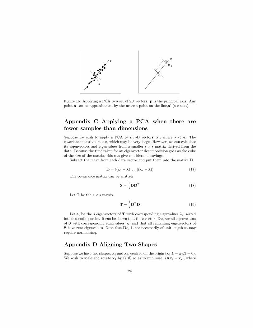
For instance, Figure 16 shows the principal axes of a 2D distribution ofvectors. In this case any of the points can be approximated by the nearest pointon the principal axis through the mean. x ≈ x′ = x+ bp where b is the distancealong the axis from the mean of the closest approach to x.

23

x

p

b

x

p

x

x’

Figure 16: Applying a PCA to a set of 2D vectors. p is the principal axis. Anypoint x can be approximated by the nearest point on the line,x′ (see text).

Appendix C Applying a PCA when there are

fewer samples than dimensions

Suppose we wish to apply a PCA to s n-D vectors, xi, where s < n. Thecovariance matrix is n×n, which may be very large. However, we can calculateits eigenvectors and eigenvalues from a smaller s × s matrix derived from thedata. Because the time taken for an eigenvector decomposition goes as the cubeof the size of the matrix, this can give considerable savings.

Subract the mean from each data vector and put them into the matrix D

D = ((x1 − x)| . . . |(xs − x)) (17)

The covariance matrix can be written

S =1

sDDT (18)

Let T be the s × s matrix

T =1

sDT D (19)

Let ei be the s eigenvectors of T with corresponding eigenvalues λi, sortedinto descending order. It can be shown that the s vectors Dei are all eigenvectorsof S with corresponding eigenvalues λi, and that all remaining eigenvectors ofS have zero eigenvalues. Note that Dei is not necessarily of unit length so mayrequire normalising.

Appendix D Aligning Two Shapes

Suppose we have two shapes, x1 and x2, centred on the origin (x1.1 = x2.1 = 0).We wish to scale and rotate x1 by (s, θ) so as to minimise |sAx1 − x2|, where

24

A performs a rotation of a shape x by θ. Let

a = (x1.x2)/|x1|2 (20)

b =

(

n∑

i=1

(x1iy2i − y1ix2i)

)

/|x1|2 (21)

Then s2 = a2 + b2 and θ = tan−1(b/a). If the shapes do not have centroidson the origin, the optimal translation is chosen to match their centroids, thescaling and rotation chosen as above.

References

[1] A. Baumberg and D. Hogg. Learning flexible models from image sequences. InJ.-O. Eklundh, editor, 3nd European Conference on Computer Vision, volume 1,pages 299–308. Springer-Verlag, Berlin, 1994.

[2] F. L. Bookstein. Principal warps: Thin-plate splines and the decomposition ofdeformations. IEEE Transactions on Pattern Analysis and Machine Intelligence,11(6):567–585, 1989.

[3] P. Burt. The pyramid as a structure for efficient computation. In A.Rosenfeld,editor, Multi-Resolution Image Processing and Analysis, pages 6–37. Springer-Verlag, Berlin, 1984.

[4] T. F. Cootes, G. J. Edwards, and C. J. Taylor. Active appearance models. InH.Burkhardt and B. Neumann, editors, 5th European Conference on ComputerVision, volume 2, pages 484–498. Springer, Berlin, 1998.

[5] T. F. Cootes and C. J. Taylor. A mixture model for representing shape varia-tion. In A. Clarke, editor, 8th British Machine Vison Conference, pages 110–119.BMVA Press, Essex, Sept. 1997.

[6] I. Dryden and K. V. Mardia. The Statistical Analysis of Shape. Wiley, London,1998.

[7] G. J. Edwards, C. J. Taylor, and T. F. Cootes. Learning to identify and trackfaces in image sequences. In 8th British Machine Vison Conference, pages 130–139, Colchester, UK, 1997.

[8] D. E. Goldberg. Genetic Algorithms in Search, Optimisation and Machine Learn-ing. Addison-Wesley, Wokingham,UK, 1989.

[9] C. Goodall. Procrustes methods in the statistical analysis of shape. Journal ofthe Royal Statistical Society B, 53(2):285–339, 1991.

[10] U. Grenander and M. Miller. Representations of knowledge in complex systems.Journal of the Royal Statistical Society B, 56:249–603, 1993.

[11] J. Haslam, C. J. Taylor, and T. F. Cootes. A probabalistic fitness measure fordeformable template models. In E. Hancock, editor, 5th British Machine VisonConference, pages 33–42, York, England, Sept. 1994. BMVA Press, Sheffield.

[12] A. Hill, T. F. Cootes, and C. J. Taylor. A generic system for image interpretationusing flexible templates. In D. Hogg and R. Boyle, editors, 3rd British MachineVision Conference, pages 276–285. Springer-Verlag, London, Sept. 1992.

25

[13] A. Hill, T. F. Cootes, and C. J. Taylor. Active shape models and the shapeapproximation problem. Image and Vision Computing, 14(8):601–607, Aug. 1996.

[14] A. Hill, T. F. Cootes, C. J. Taylor, and K. Lindley. Medical image interpretation:A generic approach using deformable templates. Journal of Medical Informatics,19(1):47–59, 1994.

[15] M. Kass, A. Witkin, and D. Terzopoulos. Snakes: Active contour models. In1st International Conference on Computer Vision, pages 259–268, London, June1987.

[16] M. Kirby and L. Sirovich. Appliction of the karhumen-loeve procedure for thecharacterization of human faces. IEEE Transactions on Pattern Analysis andMachine Intelligence, 12(1):103–108, 1990.

[17] A. Lanitis, C. J. Taylor, and T. F. Cootes. Automatic interpretation and codingof face images using flexible models. IEEE Transactions on Pattern Analysis andMachine Intelligence, 19(7):743–756, 1997.

[18] K. V. Mardia, J. T. Kent, and A. N. Walder. Statistical shape models in im-age analysis. In E. Keramidas, editor, Computer Science and Statistics: 23rd

INTERFACE Symposium, pages 550–557. Interface Foundation, Fairfax Station,1991.

[19] T. McInerney and D. Terzopoulos. Deformable models in medical image analysis:a survey. Medical Image Analysis, 1(2):91–108, 1996.

[20] W. Press, S. Teukolsky, W. Vetterling, and B. Flannery. Numerical Recipes in C(2nd Edition). Cambridge University Press, 1992.

[21] S. Solloway, C. Hutchinson, J. Waterton, and C. J. Taylor. Quantification ofarticular cartilage from MR images using active shape models. In B. Buxtonand R. Cipolla, editors, 4th European Conference on Computer Vision, volume 2,pages 400–411, Cambridge, England, April 1996. Springer-Verlag.

[22] L. H. Staib and J. S. Duncan. Boundary finding with parametrically deformablemodels. IEEE Transactions on Pattern Analysis and Machine Intelligence,14(11):1061–1075, 1992.

[23] A. L. Yuille, D. S. Cohen, and P. Hallinan. Feature extraction from faces usingdeformable templates. International Journal of Computer Vision, 8(2):99–112,1992.

26