Active Contour ModelsActive Contour Models& Active Shape Models & Active Shape Models (Snakes & Smart Snakes)(Snakes & Smart Snakes)

Image Analysis GroupImage Analysis GroupChalmers University of TechnologyChalmers University of Technology

ContentsContents

• Motivation, applications and problem description

• Active Contour Models (Snakes)

• Active Shape Models (Smart Snakes)

ApplicationsApplications

Human-computer interaction

Lip-reading

Surveillance/speed control Face recognition

Applications Applications -- MedicalMedical

Heart in ultrasound

Blood vessels

3D brain

brain in MR

Applications Applications -- Our groupOur group

Spatio-Temporal Segmentation Boundary detection

Spray segmentation

Neural cells

ProblemProblem

20 40 60 80 100 120

20

40

60

80

100

120

20 40 60 80 100 120

20

40

60

80

100

120

The basic problem is to locate an object The basic problem is to locate an object in an image (segmentation, detection)in an image (segmentation, detection)

Part IPart I

Contents for ACMContents for ACM• Active Contour Models (Snakes)

– Contour representation– Contour Energy– Formulation– Discretization– Segmentation– Notes

Contour RepresentationContour RepresentationAlthough some curves can be represented explicitly by equations of the form: 0),( =yxf

01),( 22 =−+= yxyxf

When working with complex contours usually implicit and parametric representations are used

)(xfy =)cos(xy =

)();( syysxx ==E.g. an ellipse for example is represented by

[ ]ππ, ),sin();cos( −∈== ssbysax

or...

for a parameter s.

[ ] [ ]1 ,0 ,)()()( ∈= ssysxs Tv

s=0s=1

si=0.2

y

x

v(x(si) , y(si))

x(s)

s

y(s)

ssi=0.2

si=0.2

Assign low energy values to ‘good’ contours and high energy to ‘bad’ ones

Internal energyInternal energyIn natural objects we usually require smooth contours

High energy

Low energy

Internal Energy depends on the shape of the contour itself.

s∂∂v

small

tension in the contour,low internal energy

x(s)

s

x(s)

sHigh Low

2

2

s∂∂ vsmall

No bending in the contour, low internal energy

x(s)

s

x(s)

sHigh Low

Contour Energy Contour Energy -- InternalInternal

Contour Energy Contour Energy -- ExternalExternal

When locating an object in an image...External energyExternal energy

Look for high intensity gradient (watch out for noise - gradient of smoothed image)

External Energy is derived from the image data

High energy

Low energy

could have other than gradient e.g. intensity, termination, corners...

[ ]),( yxIG ∗∇ σ

image convolved with a smoothing (ex. Gaussian) filter.

IG ∗σ

σI(x,y) image intensity

parameter controlling the extent of the smoothing (ex. variance of Gaussian).

high Low external energy

Assign low energy values to ‘good’ contours and high energy to ‘bad’ ones

Contour Energy Contour Energy -- ExamplesExampleshigh-internal energyhigh-external energy (not smooth and away from target)

high-internal energylow-external energy(not smooth and close to target)

low-internal energyhigh-external energy(smooth and away from target)

low-internal energylow-external energy(smooth and very close to target)

FormulationFormulation

first two terms:internal stretching and bending forces the third term:external forces

∫

∫

=

∂∂+

∂∂=

+=

1

0

1

0

2

2

2

2

2

1

))(()(

)()()(

)()()(

dssP

dss

sws

sw

vv

vvv

vvv

β

α

βαξ

[ ]),(),( yxIGcyxP ∗∇−= σ

[ ] [ ]1 ,0 ,)()()( ∈= ssysxs Tv

Our problem is to find the contour that minimizes the total energy (internal+external) along the contour.

In accordance with the calculus of variations, the contour must satisfy vector valued partial differential (Euler-Lagrange) equation:

w1 and w2 control the tension and rigidity

( ) 0vvv =∇+

∂∂

∂∂+

∂∂

∂∂− ))((2

2

22

2

1 sPs

wss

ws

minimization � balance of forces

DiscretizationDiscretization

Require a discrete setting:

( ) ( )

( )( ) ( )

∑∫ →

−→∂

∂=→

+

ds

ssss

Niss

ii

i

L

Kvv

vvv

1

,,2,1 ;

SegmentationSegmentation•Deform an initial contour to one having less energy.•Apply forces that decrease the energy.

Tensile force

Flexural force

Inflation force

Image force

( ) ( ) ( )112 +− −−= iiii sss vvv( ) ( ) ( )1 12i i i is s sα α α− += − −

( ) ( )( )( ) iiii sysxIqF n,=

( )( )( )

−

≥+=

otherwise 1, if 1

,TyxI

yxIF

[ ]),(),( yxIGcyxP ∗∇−= σ

( )yxPpi ,∇=

v(si+1)

v(si)

v(si-1)

Search region

p,q: constantsni: unit vector normal

to the contour at si

NotesNotes

Disadvantages of manual segmentation:•Difficult to obtain reproducible results •Operator bias•Viewing each 2D-slice separately•Operator fatigue and time consuming

Types of deformable models/active contours:•snakes •deformable templates•dynamic contours

Extensions to basic Snakes:•Inflation force (makes snake less sensitive to initial conditions)•‘dynamic programming’ and ‘simulated annealing’ (search for global minima)•Region-based image features•Changing topology

Snakes/Active contour models/deformable contour:The contour is actively changing and deforming to have less energy(deformable ~ elasticity)

Part IIPart II

Contents for ASMContents for ASM• Active Shape Models (Smart Snakes)

– Observation– Overview– Shape representation– Considerations– Training ASM– Applying ASM– Extensions

Incorporate knowledge about the desired object in the snake model

Why use the same ‘Snakes’ to locate different types of objects?

Train the snake � smart snake

ObservationObservation

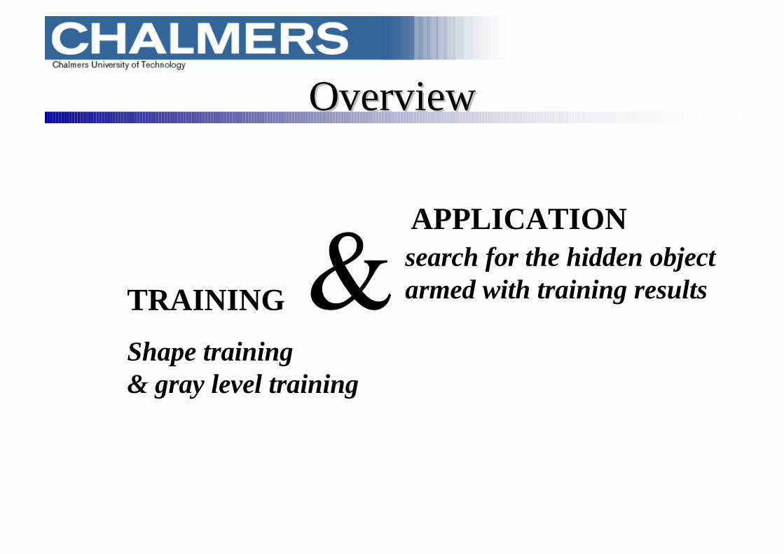
Shape training& gray level training

TRAINING

APPLICATIONsearch for the hidden objectarmed with training results

OverviewOverview

Shapes are represented by landmarks

x =

xyxy

xy

xy

k

k

1

1

2

2

16

16

M

M( , )x y16 16

Shape RepresentationShape Representation

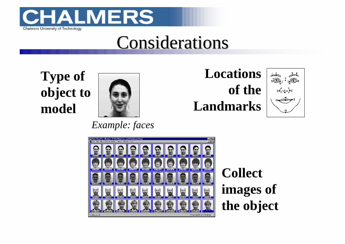
Type of object to model

Example: faces

Collect images of the object

Locations of the

Landmarks

ConsiderationsConsiderations

Study the variations of the landmark positions

Training set of images

Labeling

Shapes represented by landmarks

Aligned shapes

Aligning

Now,we can...

Shape TrainingShape Training

Capture the main modes of variation of the landmark positions

A Shapethe

mean shape

weighted sum of different shape variation modes

2Lx1 2Lx1 2Lxt tx1

Shape TrainingShape Training Result Result -- PDMPDM

Using Principal Component Analysis (PCA) we obtain the...

Point Distribution Model (PDM)

L:number of Landmarks

Rotate, scalescale, and translateto minimizethe distance

between landmarks

AligningAligning

•3D pose•Expression•Identity (subject)

Causes of variations...

Variation modesVariation modes

[ ]Ttbbb 110 ... −=b

[ ]110 ... −= tpppP

Pbxx +=

x x==∑1

1Ni

i

N

Ti

N

i

iN

))((1

1

1

xxxxCx −−−

= ∑=

[ ]Tnn yxyxyx ,,...,,,, 2211=x

P is obtained from the eigenvectors of the covariance matrix (PCA)

Constrained, only allowable variations

The corresponding eigenvalues equal the variance explained by each variation mode

iii ppCx λ=

Shape Training EquationsShape Training Equations

Study the gray levels around the landmarks

Training set of images

Shapes represented by landmarks

Extract gray level profiles around landmarks

Labeling

Now,we can...

Gray Level TrainingGray Level Training

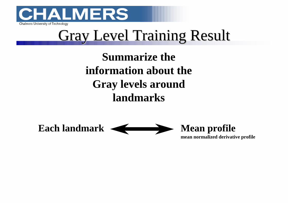
Summarize the information about the

Gray levels around landmarks

Each landmark Mean profilemean normalized derivative profile

Gray Level Training ResultGray Level Training Result

[ ]gij ij ij ijnT

g g g p= 1 2 ...

[ ]d g g g g g gij ij ij ij ij ijn ijnp pg = − − − −2 1 3 2 1...

yg

gij

ij

ijkk

n

d

dp=

=

−

∑1

1

y yji

N

ijN

==∑1

1

Gray level profile for landmark j in image i

The derivative profile for landmark j in image i

The normalized derivative profile for landmark j in image i

The mean normalized derivative profile for landmark j

Gray Level Training EquationsGray Level Training Equations

Using the shape and the gray level information to find instances of shapes in new images

Force only main modes of variation

Start with an initial shape

Search around landmarks for expected gray levelsand propose a new shape

Generally, an unallowable shapeis obtained

Find the required rotation, scaling, translation, and shape parameters updates needed to deform the current estimate to the proposed shape

Image SearchImage Search

NotesNotes

Extensions to ASMExtensions to ASM•Automatic landmark generation for PDMs•Multi resolution image search•Active Appearance Models (AAMs)•Genetic algorithms•Extension to 3D data•Other shape representations•Classification using ASM

ReferencesReferences• Image Processing, Analysis and Machine Vision. By

Sonka, Hlavac and Boyle. Second edition. PWS Publishing (pages 374-390).

• Snakes: Active Contour Models. Kass, Witkin and Terzopoulos. International Journal of Computer Vision. 1(4):321-331, 1987.

• Cootes, Taylor, Cooper and Graham. Active Shape Models - Their Training and Application. Computer Vision and Image Understanding January 1995, volume: 61, No. 1, page(s): 38-59.