An Introduction Lecture I Haye Hinrichsen DP Phase Transition DP Lattice Models Introduction Directed Percolation Outline 1 Introduction Stochastic Many-Particle Systems Equilibrium

Introduction Directed Percolation

Non-equilibrium phase transitionsAn Introduction

Lecture I

Haye Hinrichsen

University of Würzburg, Germany

March 2006


http://latex-beamer.sourceforge.net


Outline

1 IntroductionStochastic Many-Particle SystemsEquilibrium Statistical MechanicsEquilibrium and Nonequilibrium Dynamics

2 Directed PercolationFrom Isotropic to Directed PercolationThe DP Phase TransitionDP Lattice Models


Outline




Stochastic Many-Particle Systems– Basic Assumptions

Classical Statistical Physics

At a given instance of time the system is in a certainconfiguration c.

All possible configurations c form a set of configurations C.

Transitions c → c′ from one configuration to a different oneoccur spontaneously at a certain rate wc→c′ .


Transition rates

Configurations c Transition rates wc→c′


Transition rates

...trivial, but often a source of mistakes...

Rates are probabilities per unit time.

Rates carry the same dimension as 1/t .

The numerical value of a rate can be larger than 1.

In a computer simulation rates have to be multiplied by atime interval ∆t to get a probability.

if (w*dt < random(0,1)) ...


Direct Monte-Carlo Simulations

1. Choose an initial configuration and set t = 0.

2. Compute total outgoing rate Wc =∑

c′∈C wc→c′ .

3. Select new configuration c′ with probability wc→c′/Wc .

4. Increase t by 1/Wc*.

5. Monitor quantities of interest and continue while t < tmax .

* Approximation, good if t � 1/Wc


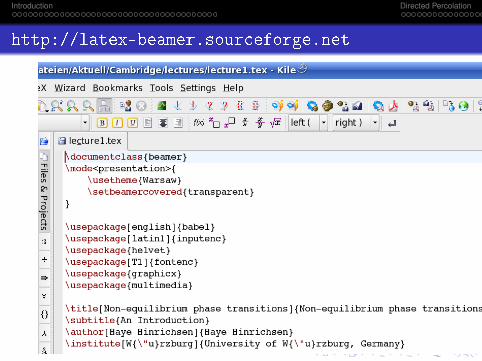
Direct Monte-Carlo Simulations

Approximation:

Poisson statistics (like radioactive decay) → regular intervals


Time-dependent Probability Distribution

The individual trajectory of aclassical stochastic system is unpredictable.

Probability Distribution

Pt(c) is the probability to find the system at time tin the configuration c.∑

c∈CPt(c) = 1

The evolution of Pt(c) is predictable.


Master Equation

The master equation is a linear deterministic evolutionequation that describes the flow of probability:

∂

∂tPt(c) =

∑c′

wc′→cPt(c′)︸︷︷︸gain

−∑c′

wc→c′Pt(c)︸︷︷︸loss

.

In the continuum also called Fokker-Planck equation.(do not mix up with Langevin equations, see below.)


Compact Notation – Time Evolution Operator

List all the probabilities in a vector:

|Pt〉 =

Pt(c1)Pt(c2)Pt(c3). . .

∈ [0,1]⊗|C|

Write Master equation in a compact form:

∂t |Pt〉 = −L|Pt〉

L is called Liouville operator.


Compact Notation – Formal Solution

The Lioville operator L is defined by the matrix elements

〈c′|L|c〉 = −wc→c′ + δc,c′∑c′′

wc→c′′ .

Formal solution:|Pt〉 = e−Lt |P0〉 ,

where |P0〉 is the initial probability distribution at t = 0

...looks like quantum mechanics...


Compact Notation – Conservation of Probability

Probability conservation ∑c∈C

Pt(c) = 1

can be expressed as〈1|Pt〉 = 1 ,

where〈1| :=

∑c∈C

〈c| = (1,1,1,1, . . . ,1)

⇒〈1|L = 0


Compact Notation – Structure of L

The matrix of the time evolution operator in configuration basis

has positive entries on the diagonal,has negative non-diagonal entries,and the sum over columns vanishes.

Example: L =

2 −3 −5−1 5 −1−1 −2 6

Such matrices are called intensity matrices.


Solving the Master Equation by Diagonalization

The master equation can be solved by diaogalization of L:1. Solve eigenvalue problem:

L|φi〉 = λi |φi〉

2. Express initial state |P0〉 in terms of eigenvectors:

|P0〉 =∑

i

ai |φi〉

3. Write down the solution:

|Pt〉 = e−Lt |P0〉 =∑

i

ai e−λi t |φi〉

solution = sum over exponentially decaying eigenmodes


Spectrum of the Time Evolution Operator

The time evolution operatoris non-Hermitean, meaning that left and right eigenvectorsto the same eigenvalue may have different representations.

Because of 〈1|L = 0 there is at least one eigenvalueλ0 = 0, representing the stationary state.

All eigenvalues have a non-negative real part.

Eigenvalues may occur in complex-conjugate pairs.

complex? damped oscillations?


Complex Eigenvalues of L – Chemical Oscillations

Belusov-Zhabotinsky-Reaction

http://online.redwoods.cc.ca.us/instruct/darnold/deproj/


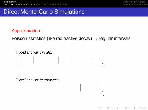
Complex Eigenvalues - Chemical Oscillations

Chemical oscillations occur in activator-inhibitorreactions:


Complex Conjugate Eigenvalues - ChemicalOscillations

Even spatio-temporal oscillations can be observed...


Complex Conjugate Eigenvalues - ChemicalOscillations

...and may be simulated by partial differential equations:


Classical Stochastic Dynamics compared toQuantum Mechanics

Quantum Mechanics∫ψ∗(x)ψ(x)dx = 1 〈ψ|ψ〉 = 1 H = H† U−1 = U†

Classical Stochastic Dynamics∑c Pt(c) = 1 〈1|Pt〉 = 1 〈1|L = 0 〈1|U = U

...look similar, but differ significantly.



Relaxation times

The relaxation time of an eigenmode |φi〉 is (Reλi)−1

Systems with finite configuration space relax to theirstationary state exponentially within finite timedetermined by the eigenvalue with the smallest real part.

Conversely: Systems exhibiting infinite relaxation times orpower laws must have an infinite configuration space.



Relaxation times






Relaxation times





Outline




System in Equilibrium with a Heat Bath


Temperature

In equilibrium Nature maximizes theentropy S of the entire system.

The total entropy is extensive: S = S1 + S2

The total energy is conserved: E = E1 + E2

⇒ ∂S1

∂E1= −∂S1

∂E1=∂S2

∂E2

⇒ The quantity 1T := ∂S

∂E is the same in both subsystems.

Temperature ⇔ equilibrium & energy conservation.


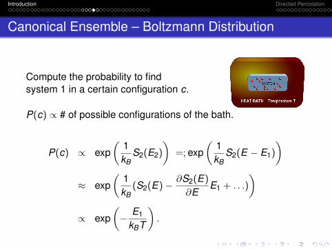
Canonical Ensemble – Boltzmann Distribution

Compute the probability to findsystem 1 in a certain configuration c.

P(c) ∝ # of possible configurations of the bath.

P(c) ∝ exp(

1kB

S2(E2)

)=; exp

(1kB

S2(E − E1)

)

≈ exp(

1kB

(S2(E)− ∂S2(E)

∂EE1 + . . .)

)

∝ exp(− E1

kBT

).


Equilibrium Statistical Mechanics

In equilibrium statistical mechanicsthere is no notion of time.

Equilibrium models are defined by anenergy functional c → E(c).

In equilibrium statistical mechanics we getthe probability distribution for free!

——————————————————–

Nonequilibrium models are defined by aset of transition rates.

In nonequilibrium statistical mechanicsthe probability distribution is obtainedby solving the master equation.


Outline




Equilibrium and Nonequilibrium Dynamics

There are two types of stochastic dynamical processes:

1 Equilibrium dynamics:Dynamical processes which relax towards a stationarystate described by an equilibrium ensemble.

2 Nonequilibrium dynamics:All other processes.








Equilibrium Dynamics

Example:The following dynamical processes

1 Ising Heat bath dynamics2 Glauber-Ising model3 Ising Metropolis dynamics4 Ising Kawasaki dynamics∗5 Swendsen-Wang cluster algorithm6 Wolf cluster algorithm7 · · ·

relax towards a stationary state which is precisely theequilibrium ensemble of the Ising model.

Proof needed!


Detailed Balance

A system is said to obey Detailed Balance if the probabilitycurrents between pairs of configurations compensate eachother:

Peq(c) wc→c′ = Peq(c′) wc′→c .


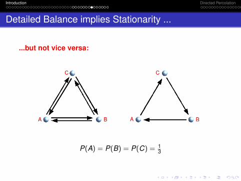
Detailed Balance implies Stationarity ...

...but not vice versa:

P(A) = P(B) = P(C) = 13


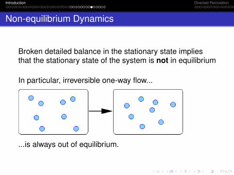
Non-equilibrium Dynamics

Broken detailed balance in the stationary state impliesthat the stationary state of the system is not in equilibrium

In particular, irreversible one-way flow...

...is always out of equilibrium.


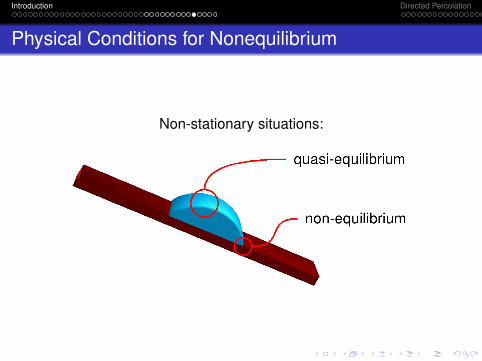
Physical Conditions for Nonequilibrium

Non-stationary situations:



Flow of energy through the system:



Flow of particles through the system:


Continuous Phase Transitions

Continuous phase transitions at equilibrium:

can be categorized into universality classes .

are particularly well understood in two dimensions,where conformal invariance leads to a classificationscheme.

Nonequilibrium phase transitions ?


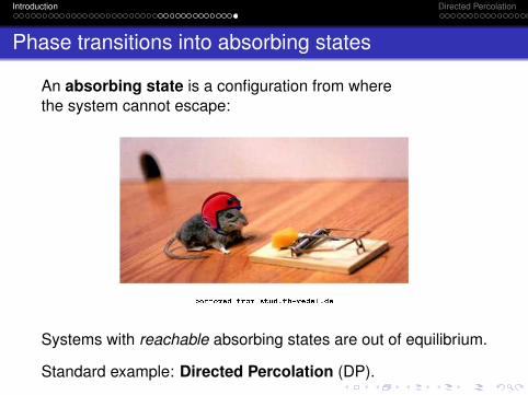
Phase transitions into absorbing states

An absorbing state is a configuration from wherethe system cannot escape:

borrowed from stud.fh-wedel.de

Systems with reachable absorbing states are out of equilibrium.

Standard example: Directed Percolation (DP).


Outline




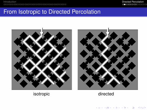
From Isotropic to Directed Percolation

isotropic directed


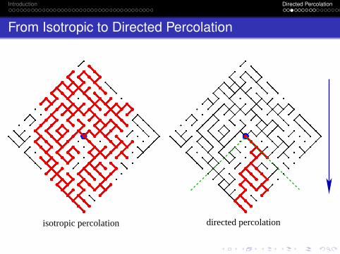
From Isotropic to Directed Percolation

isotropic percolation directed percolation


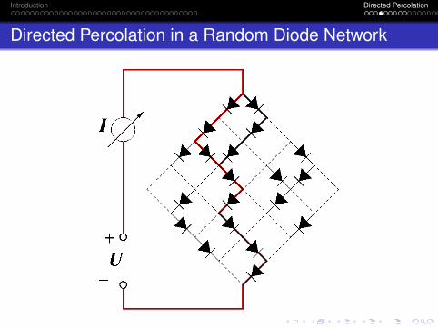
Directed Percolation in a Random Diode Network


Directed Percolation as a Dynamical Process

The preferred direction can be interpreted as time t .


DP is easy to simulate


DP is easy to simulate


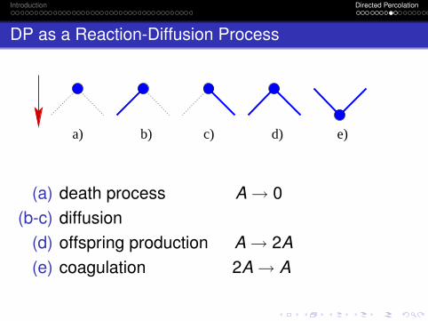
DP as a Reaction-Diffusion Process

a) b) c) d) e)

(a) death process A → 0(b-c) diffusion

(d) offspring production A → 2A(e) coagulation 2A → A


DP as a Simple Model for Epidemic Spreading


Outline




DP exhibits a Phase Transition

...starting with a fully active lattice:


DP exhibits a Phase Transition

...starting with a single active site:


Order Parameter: Number of Active Sites N(t)

Let us measure 〈N(t)〉 for various q.


This little program does it:

#include <fstream.h>using namespace std;const int T=1000; // number of updatesconst int R=10000; // number of independent runsconst double p=0.6447; // percolation probability

double rnd(void) { return (double)rand()/0x7FFFFFFF; }

int main (void){int s[T][T],N[t]i,t,r;for (t=0; t<T; t++) N[t]=0; // clear cumulative particle numberfor (r=0; r<R; r++) { // loop over R runs

s[0][0]=1; // place initial seedfor (t=0; t<T-1; t++) { // temporal loop

for (i=0; i<=t+1; ++i) s[t+1][i]=0; // clear new configfor (i=0; i<=t; ++i) if (s[t][i]==1) { // loop over active sites

N[t]++; // count active sitesif (rnd()<p) s[t+1][i]=1; // random activation leftif (rnd()<p) s[t+1][i+1]=1; // random activation right

} } }ofstream os ("N.dat"); // write average N(t) to filefor (t=0; t<T-1; t++) os << t << ' ' << (double)N[t]/R << endl;}


This is the Output (via xmgrace):

1 10 100 1000t

0,01

0,1

1

10

100

<N

(t)>

p=0.7p=0.65p=0.6447 (critical)p=0.64p=0.6

0 100 300 400t10

-2

10-1

100

<N

(t)>


Result for 〈N(t)〉:

For q < qc 〈N(t)〉 crosses over to an exponential decay.

For q > qc 〈N(t)〉 tends to a linear increase.

At q = qc 〈N(t)〉 increases algebraically as tθ

with an exponent θ ≈ 0.302.


WARNING: NEVER use the Standard Deviation:


UNIVERSALITY

The exponent

θ = 0.313686(8)

is the same in all realizations of DP.It only depends on the dimension d .

DP stands for a universality classof non-equilibrium phase transitions.

DP is the ’Ising model’ of non-equilibrium.


UNIVERSALITY

All long-range properties, especially critical exponentsand scaling functions, are universal, i.e., they are thesame for all models in the DP universality class.

Short-range properties and critical threshold (pc) arenon-universal.

→ Examples of different DP models?→ Can we characterize the range of DP models?


Outline




DP Lattice Models


Domany-Kinzel Cellular Automaton

Transition probabilities:

P[1|0,0] = 0P[1|0,1] = P[1|1,0] = p1

P[1|1,1] = p2



p 2p1s p 1i

t+1

t

i-1s i+1s

Algorithm:

For all i generate a random number zi ∈ [0,1] and set:

si(t + 1) =

1 if si−1(t) 6= si+1(t) and zi(t) < p1 ,1 if si−1(t) = si+1(t) = 1 and zi(t) < p2 ,0 otherwise .



Special cases:

case restriction p1,c p2,c

Wolfram 18 p2 = 0 0.801(2) 0

Site DP p2 = p1(2− p1) 0.70548515(20) 0.70548515(20)

Bond DP p1 = p2 0.644700185(5) 0.873762040(3)

Compact DP p2 = 1 1/2 1


Domany-Kinzel Model: Phase Diagram

0 1p

1

0

1

p2

inactive phase

activephase

compact DP

bond DP

site DP

rule 18Wolfram


Domany-Kinzel Model: Phase Diagram

site DP bond DP compact DPWolfram 18

Compact DP is not DPbut it is the same as Glauber-Ising at T = 0.

All the rest of the transition line belongs to DP.


Two-dimensional Domany-Kinzel model

t


End of Part I

Documents

An Introduction Lecture I Haye Hinrichsen DP Phase Transition DP Lattice Models Introduction Directed Percolation Outline 1 Introduction Stochastic Many-Particle Systems Equilibrium