Embed Size (px)
Citation preview


ESCUELA TÉCNICA SUPERIOR DE INGENIEROS DE MONTES
UNIVERSIDAD POLITÉCNICA DE MADRID
AN INTEGRAL MODEL FOR NATURAL
REGENERATION OF Pinus pinea L. IN THE NORTHERN
PLATEAU (SPAIN)
-
MODELO INTEGRAL DE REGENERACIÓN NATURAL
PARA Pinus pinea L. EN LA MESETA NORTE (ESPAÑA)
TESIS DOCTORAL
RUBÉN MANSO GONZÁLEZ
Ingeniero de Montes
MADRID, 2012


PROGRAMA DE DOCTORADO DE SILVOPASCICULTURA
ESCUELA TÉCNICA SUPERIOR DE INGENIEROS DE MONTES
UNIVERSIDAD POLITÉCNICA DE MADRID
AN INTEGRAL MODEL FOR NATURAL
REGENERATION OF Pinus pinea L. IN THE NORTHERN
PLATEAU (SPAIN)
-
MODELO INTEGRAL DE REGENERACIÓN NATURAL
PARA Pinus pinea L. EN LA MESETA NORTE (ESPAÑA)
RUBÉN MANSO GONZÁLEZ
Ingeniero de Montes
DIRECTORES
MADRID, 2012
MARTA PARDOS MÍNGUEZ
Doctora Ingeniera de Montes
RAFAEL CALAMA SÁINZ
Doctor Ingeniero de Montes


Tribunal nombrado por el Mgfco. y Excmo. Sr. Rector de la Universidad Politécnica
de Madrid, el día………de………………de 2012
Presidente D. …………………………………
Vocal D. …………………………………
Vocal D. …………………………………
Vocal D. …………………………………
Secretario D. …………………………………
Realizado el acto de defensa y lectura de la Tesis el día………de ………………de
2013 en ………………..
Calificación…………………………
EL PRESIDENTE LOS VOCALES
EL SECRETARIO


La presente tesis ha sido financiada dentro del marco funcional del proyecto
RTA 2007-00044 del Instituto Nacional de Investigación y Tecnología Agraria y
Alimentaria (INIA)


i
Contents Resumen ......................................................................................................................... v
Abstract ........................................................................................................................ vii
1. Introduction ................................................................................................................ 1
1.1. Pinus pinea ethnobotany ..................................................................................... 3 1.2. Pinus pinea in the Northern Plateau of Spain ..................................................... 4 1.3. Regeneration of Pinus pinea in managed forests of the Northern Plateau ......... 7 1.4. Reproductive ecology of Pinus pinea ............................................................... 10 1.5. A model for natural regeneration of Pinus pinea .............................................. 12 1.6. Study site ........................................................................................................... 14 1.7. Objectives and organization .............................................................................. 16 References ................................................................................................................ 18
2. Primary dispersal ..................................................................................................... 23
2.1. Abstract ............................................................................................................. 27 2.2. Introduction ....................................................................................................... 28 2.3. Material and methods ........................................................................................ 31
2.3.1. Study site .................................................................................................... 31 2.3.2. Experimental design................................................................................... 32 2.3.3. Modelling the spatial pattern ..................................................................... 32 2.3.4. Modelling the temporal pattern .................................................................. 37
2.4. Results ............................................................................................................... 38 2.4.1. Seed rain..................................................................................................... 38 2.4.2. Spatial pattern ............................................................................................ 39 2.4.3. Temporal pattern ........................................................................................ 42
2.5. Discussion ......................................................................................................... 43 2.5.1. The inverse modelling approach ................................................................ 43 2.5.2. Model improvements ................................................................................. 45 2.5.3. Spatial pattern of seed dispersal ................................................................. 46 2.5.4. Temporal pattern of seed dispersal ............................................................ 47 2.5.5. Management implications .......................................................................... 48
References ................................................................................................................ 49 3. Seed germination ..................................................................................................... 53
3.1. Abstract ............................................................................................................. 57 3.2. Introduction ....................................................................................................... 58 3.3. Material and methods ........................................................................................ 60
3.3.1. Study area................................................................................................... 60 3.3.2. Experimental design................................................................................... 61 3.3.3. Survival analysis ........................................................................................ 63 3.3.4. Hazard function definition ......................................................................... 64 3.3.5. Likelihood function formulation ................................................................ 66 3.3.6. Model fitting and evaluation ...................................................................... 67
3.4. Results ............................................................................................................... 68 3.4.1. Hazard function .......................................................................................... 68 3.4.2. Optimum conditions for germination......................................................... 69

ii
3.4.3. Model evaluation ....................................................................................... 72 3.5. Discussion ......................................................................................................... 72
3.5.1. Modelling approach ................................................................................... 72 3.5.2. Pinus pinea case study ............................................................................... 75
References ................................................................................................................ 77 4. Seed predation and secondary dispersal .................................................................. 81
4.1. Abstract ............................................................................................................. 85 4.2. Introduction ....................................................................................................... 86 4.3. Material ............................................................................................................. 88
4.3.1. Study site .................................................................................................... 88 4.3.2. Experimental design................................................................................... 89
4.4. Methods............................................................................................................. 91 4.4.1. Camera sightings ........................................................................................ 91 4.4.2. Seed removal .............................................................................................. 92 4.4.3. Seed fate ..................................................................................................... 96
4.5. Results ............................................................................................................... 96 4.5.1. Camera sightings ........................................................................................ 96 4.5.2. General pattern of seed removal ................................................................ 97 4.5.3. Seed removal model ................................................................................... 98 4.5.4. Seed fate ................................................................................................... 101
4.6. Discussion ....................................................................................................... 102 4.6.1. The role of A. sylvaticus in P. pinea natural regeneration ....................... 102 4.6.2. Seed removal ............................................................................................ 103 4.6.3. Secondary seed dispersal ......................................................................... 104 4.6.4. The Apodemus sylvaticus-Pinus pinea interaction .................................. 106
References .............................................................................................................. 108 5. Seedling survival .................................................................................................... 115
5.1. Abstract ........................................................................................................... 117 5.2. Introduction ..................................................................................................... 118 5.3. Material and methods ...................................................................................... 118
5.3.1. Study site .................................................................................................. 118 5.3.2. Experimental design................................................................................. 119 5.3.3. Modelling approach ................................................................................. 119
5.4. Results ............................................................................................................. 121 5.5. Discussion ....................................................................................................... 123 References .............................................................................................................. 125
6. Multistage stochastic model ................................................................................... 127
6.1. Abstract ........................................................................................................... 131 6.2. Introduction ..................................................................................................... 132 6.3. Material and methods ...................................................................................... 134
6.3.1. Regeneration model ................................................................................. 134 6.3.2. Stochastic simulation ............................................................................... 138 6.3.3. Stochastic optimisation ............................................................................ 141
6.4. Results ............................................................................................................. 143 6.4.1. Stochastic simulations .............................................................................. 143 6.4.2. Optimisation ............................................................................................. 147

iii
6.5. Discussion ....................................................................................................... 150 6.5.1. Stochastic simulations and stochastic optimisation ................................. 150 6.5.2. Current implications for management ..................................................... 152 6.5.3. Future climate and future management.................................................... 153
References .............................................................................................................. 157 7. Conclusions ............................................................................................................ 161
Epílogo ....................................................................................................................... 167

iv
v
Resumen
La regeneración natural es un proceso ecológico clave que posibilita la
persistencia de las especies vegetales y, por tanto, representa un elemento de gran
relevancia para la gestión forestal sostenible. Sin embargo, la regeneración natural en
rodales regulares de Pinus pinea L. de la Meseta Norte (España) no siempre se consigue
de forma satisfactoria, a pesar de más de un siglo de gestión centrada en la producción
de piñón. Como consecuencia, la regeneración natural es en la actualidad una cuestión
de gran interés para los gestores, en un momento de racionalización de los recursos
destinados a la gestión forestal. Mediante la presente tesis se pretende ofrecer respuestas
en este sentido al gestor mediante el desarrollo de un modelo integral multietápico de
regeneración para rodales del P. pinea de la Meseta Norte. A partir de este modelo se
pueden derivar recomendaciones para una selvicultura basada en la regeneración natural
bajo el clima actual y también considerando escenarios climáticos futuros. Además, la
estructura del modelo permite la detección de los cuellos de botella que pudieran afectar
al proceso. El modelo integral consta de cinco submodelos correspondientes a cada uno
de los subprocesos que ligan las diferentes fases de la regeneración natural (producción
de semillas, dispersión, germinación, predación y supervivencia del regenerado). Las
salidas de los submodelos representan las probabilidades de transición entre estas fases
en función de variables climáticas y de masa que, a su vez, recogen el efecto de los
factores ecológicos que gobiernan el proceso de regeneración. A nivel de subproceso,
los resultados de esta tesis deben interpretarse como sigue. La programación de las
cortas del aclareo sucesivo uniforme que se viene aplicando en rodales altamente
aclarados induce a una limitación por dispersión desde las primeras fases del periodo de
regeneración. En lo relativo a la predación, la actividad de los predadores aparentemente
sólo queda condicionada por las intensas sequías estivales y los eventos veceros, de
donde se deduce que el verano es un periodo seguro para las semillas. Fuera de este
periodo, la práctica totalidad de las semillas son consumidas. Dado que la diseminación
en P. pinea se produce en verano (el periodo seguro para las semillas), la probabilidad
de que una semilla no sea destruida depende de que la germinación tenga lugar con
anterioridad a la reactivación de la actividad predadora. Sin embargo, las condiciones
óptimas para la germinación no se dan de forma habitual, limitando la emergencia a
unos pocos días durante el otoño. En suma, existe una ventana muy estrecha para
vi
alcanzar la fase de plántula. Además, el submodelo de supervivencia del regenerado
predice tasas de mortalidad de plántulas extremadamente altas y por tanto sólo algunos
individuos de cohortes numerosas podrán instalarse definitivamente. Estas
circunstancias, junto con el fuerte carácter vecero de P. pinea, controlado por factores
climáticos, indican que la probabilidad final de establecimiento es baja. Partiendo de
estas circunstancias, la gestión actual –bajas densidades como consecuencia de claras
intensas y un esquema de regeneración estricto– condiciona la ocurrencia de un número
suficiente de eventos favorables para la consecución de la regeneración natural durante
el periodo de regeneración actual. Las simulaciones y optimización estocástica que se
han llevado a cabo por medio del modelo integral confirman este extremo, sugiriendo
que los tratamientos de regeneración deberían ejecutarse de forma más flexible y
progresiva. Desde un punto de vista ecológico, estos resultados son informativos de una
estrategia reproductiva que implica una estructura irregular de masa, en la línea de lo
que podría deducirse del temperamento medianamente tolerante de la especie. Como
observación final, las simulaciones estocásticas realizadas bajo un escenario de cambio
climático muestran que la regeneración en la especie no se verá fuertemente afectada en
el futuro. Este comportamiento resiliente refuerza el fundamental papel ecológico que
juega P. pinea en áreas donde la severas condiciones ambientales impiden la
persistencia de otras especies arbóreas.

vii
Abstract
Natural regeneration is an ecological key-process that makes plant persistence
possible and, consequently, it constitutes an essential element of sustainable forest
management. In this respect, natural regeneration in even-aged stands of Pinus pinea L.
located in the Spanish Northern Plateau has not always been successfully achieved
despite over a century of pine nut-based management. As a result, natural regeneration
has recently become a major concern for forest managers when we are living a moment
of rationalization of investment in silviculture. The present dissertation is addressed to
provide answers to forest managers on this topic through the development of an integral
regeneration multistage model for P. pinea stands in the region. From this model,
recommendations for natural regeneration-based silviculture can be derived under
present and future climate scenarios. Also, the model structure makes it possible to
detect the likely bottlenecks affecting the process. The integral model consists of five
submodels corresponding to each of the subprocesses linking the stages involved in
natural regeneration (seed production, seed dispersal, seed germination, seed predation
and seedling survival). The outputs of the submodels represent the transitional
probabilities between these stages as a function of climatic and stand variables, which in
turn are representative of the ecological factors driving regeneration. At subprocess
level, the findings of this dissertation should be interpreted as follows. The scheduling
of the shelterwood system currently conducted over low density stands leads to
situations of dispersal limitation since the initial stages of the regeneration period.
Concerning predation, predator activity appears to be only limited by the occurrence of
severe summer droughts and masting events, the summer resulting in a favourable
period for seed survival. Out of this time interval, predators were found to almost totally
deplete seed crops. Given that P. pinea dissemination occurs in summer (i.e. the safe
period against predation), the likelihood of a seed to not be destroyed is conditional to
germination occurrence prior to the intensification of predator activity. However, the
optimal conditions for germination seldom take place, restraining emergence to few
days during the fall. Thus, the window to reach the seedling stage is narrow. In addition,
the seedling survival submodel predicts extremely high seedling mortality rates and
therefore only some individuals from large cohorts will be able to persist. These facts,
along with the strong climate-mediated masting habit exhibited by P. pinea, reveal that

viii
the overall probability of establishment is low. Given this background, current
management –low final stand densities resulting from intense thinning and strict felling
schedules– conditions the occurrence of enough favourable events to achieve natural
regeneration during the current rotation time. Stochastic simulation and optimisation
computed through the integral model confirm this circumstance, suggesting that more
flexible and progressive regeneration fellings should be conducted. From an ecological
standpoint, these results inform a reproductive strategy leading to uneven-aged stand
structures, in full accordance with the medium shade-tolerant behaviour of the species.
As a final remark, stochastic simulations performed under a climate-change scenario
show that regeneration in the species will not be strongly hampered in the future. This
resilient behaviour highlights the fundamental ecological role played by P. pinea in
demanding areas where other tree species fail to persist.

ix
“Mais les destins se forment lentement et nul ne sait, parmi tous nos actes semés au
hasard, lesquels germeront pour s’épanouir, comme des arbres”
Maurice Druon
Les rois maudits

x

Chapter 1 Introduction
1. Introduction


–––––––––––––––––––––––––––––––––––––––––––––––– Chapter 1: Introduction
3
1. Introduction
1.1. Pinus pinea ethnobotany
Pinus pinea L., the Mediterranean stone pine, is one of the most emblematic
Mediterranean plant species. Its current distribution in the Mediterranean area
comprises forests that, although sparse, are widely spread all over the northern shore of
the Mediterranean basin, from Lebanon to Portugal. Easily recognizable at first glance
for its distinctive umbrella-like crown, P. pinea is acknowledged as a structural element
of the Mediterranean landscape. The species is remarkably plastic in the Mediterranean
context, able to bear severe and persistent droughts, relatively extreme temperatures as
well as poor and sandy soils. These features inform a valuable ecological role of P.
pinea, which can occur in limiting sites, even where other tree species fail to persist. In
this respect, P. pinea has been reported to provide shelter and food to wild and
endangered fauna (SEO/BirdLife, 1999), to protect watershed and soil and to efficiently
stabilize dunes (Montero et al., 2008). However, it is the edible and highly nutritious
seed born by its cones (pine nuts, pinyons, piñons, pignons) what renders P. pinea an
inseparable companion of Mediterranean inhabitants from ancient times. Indeed, pine
nuts from P. pinea have been exploited by human communities since the Palaeolithic
era, as demonstrated by the findings from various archaeological sites (Carrión et al.,
2008).
Because P. pinea has been so intimately present in human ecohistory, it is
difficult –not to say impossible– to precisely determine its original distribution area.
Both accidental and intentional installation due to human transit and trade, taking place
since Neolithic times 6,000 years BP (Earle, 2011), may have favoured the occurrence
of the species in the northern Mediterranean. In addition, modern protective and
productive plantations have extended the presence of P. pinea within the boundaries of
the Mediterranean basin (up to 0.7 million hectares) but also beyond them as far as
Chile, Argentina, South Africa or Australia (Mutke et al., 2012) .
Nevertheless, there is overwhelming abundance of macrofossil and
palynological records that confirm the presence of P. pinea as a native species or a
protohistoric archeophyte throughout all the current Mediterranean distribution area
during the Holocene (Feinbrun, 1959; Franco-Múgica et al., 2005; García-Amorena et
al., 2007; Henri et al., 2010, among many others) and even before and during the Last
–––––––––––––––––––––––––––––––––––––––––––––––– Chapter 1: Introduction
4
Glacial Maximum (50,000–18,000 years BP; Bazile-Robert (1981); Carrión et al.
(2008)). The recent finding of a practically null genetic variation between and within
populations suggests that the species experienced a rigorous and prolonged
demographic bottleneck before its quaternary expansion (Vendramin et al., 2008). This
fact gives rise to the hypothesis that the species already occupied southern European
areas in the upper Tertiary, as confirmed by the studies by Menéndez-Amor (1951) and
Klaus (1989) in the Iberian Peninsula and Austria, respectively.
A detailed review on P. pinea natural and cultural history can be found in Mutke
et al. (2012).
1.2. Pinus pinea in the Northern Plateau of Spain
The Northern Plateau of Spain is located in north central Iberian Peninsula. It
consists of an inland tableland of about 50,000 km2 at a mean altitude of 700 m above
sea level surrounded by mountain ranges. The latitude of the plateau determines its
Mediterranean-dominant climate, mainly evidenced by the occurrence of severe, four-
month summer droughts. In this context, its sheltered physiographic situation, which
prevents the ocean humid influence, leads to low mean precipitation values (ranging
from 300 to 500 mm), only higher in the Iberian Peninsula than those recorded in the
semi-desert southeasternmost areas (AEMET-IM, 2011). In addition, its relatively high
elevation conditions the winter period, colder than in most of the peninsular territory
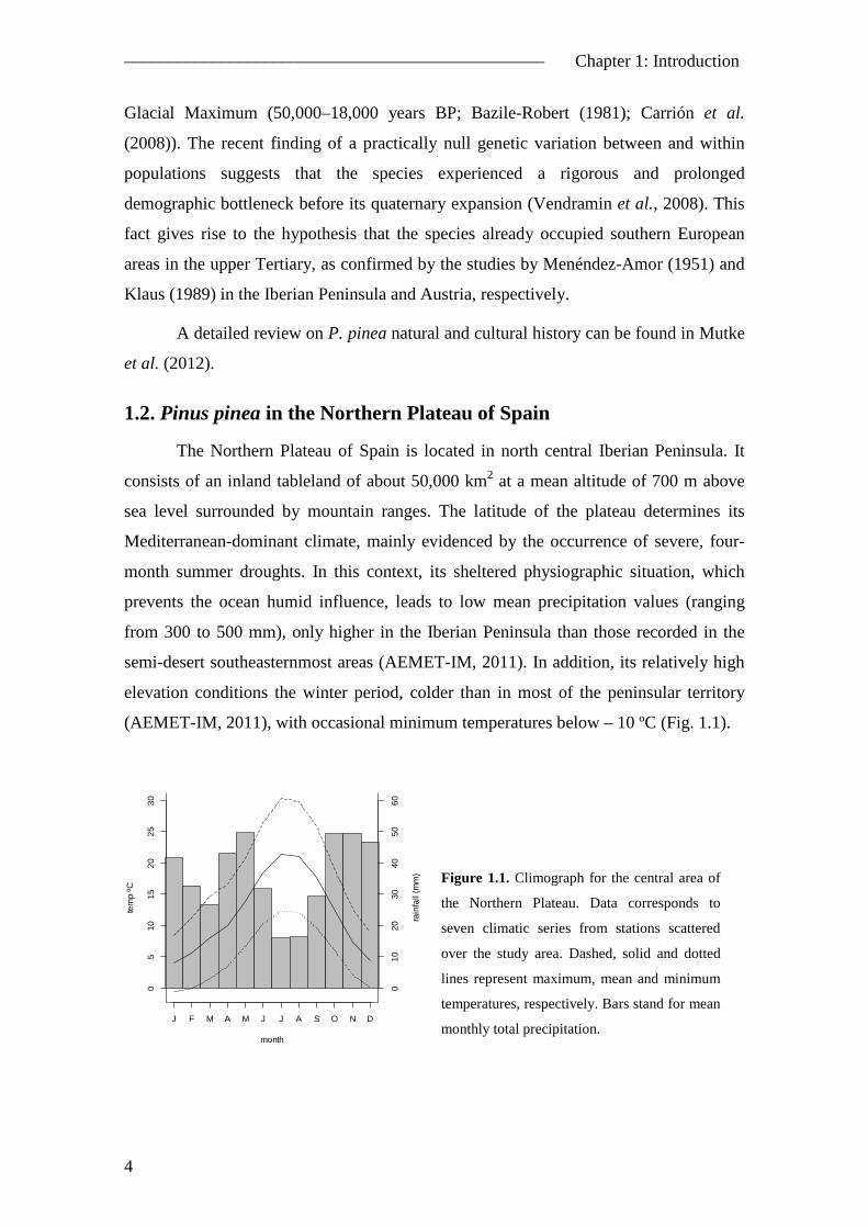
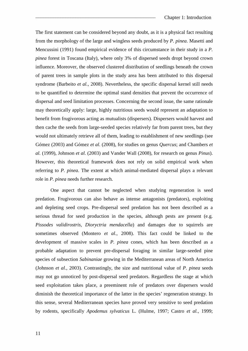
(AEMET-IM, 2011), with occasional minimum temperatures below – 10 ºC (Fig. 1.1).
month
tem
p ºC
05
1015
2025
30
J F M A M J J A S O N D
010
2030
4050
60
rain
fall
(mm
)
Figure 1.1. Climograph for the central area of
the Northern Plateau. Data corresponds to
seven climatic series from stations scattered
over the study area. Dashed, solid and dotted
lines represent maximum, mean and minimum
temperatures, respectively. Bars stand for mean
monthly total precipitation.

–––––––––––––––––––––––––––––––––––––––––––––––– Chapter 1: Introduction
5
Northern Plateau’s origin dates from the late Mesozoic and early Cenozoic,
when the Alpine orogeny (65–100 Ma BP) produced the depression of the territories
corresponding to central Iberian Peninsula nowadays. During the Miocene (23–5 Ma
BP), the sediments of an inland lake gave rise to a calcareous plain, origin, in turn, of
the Duero River basin. Later, during the Pleistocene (2,588–11.7 ka BP), Duero
tributaries flowing northwards through the plateau from the Central Range deposited an
important amount of eroded siliceous materials, which were ultimately spread by
aeolian erosion. As a result of these processes, the areas located between the Duero
River and the Central Range are presently dominated by two main units: limestone flat
uplands and sandy plains. It is in these areas where one of the more extensive Iberian P.
pinea woodlands currently lies (over 50,000 ha; Gordo et al. (2012)) and consequently
named after as Tierra de Pinares (Pinewoods Land; Fig. 1.2).
Although the occurrence of P. pinea in the Iberian Peninsula during the
Pleistocene is widely accepted, there is not a general agreement on the naturalness of
the species in the Northern Plateau, probably as a result of a divergence on the
approaches to interpret the past landscape (see Navarro and Valle (1987) and Rivas-
Martínez (2007) for a geographical and phytosociological approach, respectively).
However, the persistence of the species both in the limestone and sandy environments
of the region, at least throughout the Holocene, can no longer be ignored, as supported
by the palynological analyses by Franco-Múgica et al. (2001; 2005). Moreover, the
findings by Rubiales et al. (2011) and Hernández et al. (2011) based on macro-remains
indubitably indicate the intense use of P. pinea resources by pre-Roman populations
about 2500 years BP.
Figure 1.2. Location of the Northern Plateau in the Iberian context (left) and natural distribution of
Pinus pinea in the Northern Plateau (right). Source: INIA

–––––––––––––––––––––––––––––––––––––––––––––––– Chapter 1: Introduction
6
Natural occurrence of pure stands of P. pinea is unlikely in the Northern Plateau,
except when very specific soil and climate conditions take place (Gordo et al., 2012).
Ideally, the species would grow intimately associated to Pinus pinaster Ait. when
highly sandy soils are present and to Quercus ilex, Quercus faginea, Juniperus
thuriphera and Juniperus communis on limestone uplands (Clément, 1993; Franco-
Múgica et al., 2001; Franco-Múgica et al., 2005). This landscape must be what Roman
invaders found in the area in the 2nd century BC. According to Apiano’s chronicles
(151 BC), pinewoods located southwards Duero River were not severely altered by
Celtiberian Vaccaean indigenous tribes, in contrast to the total deforestation
accomplished over the northern shore as a result of its superior quality as agricultural
land and grassland (Hopfner, 1954). Human pressure on these forests during the Roman
domination (2nd century BC to 5th century AC) and the Visigoth period (5th–7th
century AC) was most probably neither drastic nor irreversible, given the persistence of
dense woodlands used as a “convenient unpopulated border” (the so called “Duero
desert”) between Arabians and Christians until the 11th century (Clément, 1993). After
the taking of Toledo by Christians in 1085, the first permanent settlements were
established in the area and a period of increasing transformation of woodlands, normally
communal, into agrarian exploitations took place. This deforestation process was
augmented as a result of the privileges bestowed by the Castilian Crown to grazing
activities after the 13th century. Contemporary to this change in land uses, the density
of P. pinea within pinewoods notably decreased due to the uncontrolled timber
extraction from this species, given its higher adequacy as lumber over the wood from P.
pinaster (Gordo et al., 2000). As a consequence of the higher power concentration on
the Monarchy after the 15th century (and especially during the 18th century), different
laws and rules were passed as an attempt to protect these forests and particularly P.
pinea individuals, reaching different degrees of success (Guerra, 2001). However, the
liberal thought arising by the half of the 19th century in Spain along with the
complicated situation of the Public Treasure, led the State to confiscate, among many
other goods, an important fraction of communal forests for immediate selling, which in
many cases also implied immediate logging. Had not been for the new conservationist
concerns that simultaneously appeared in opposition to the confiscation law of 1855, P.
pinea forests would have been seriously endangered. Efforts were not spared by forest
managers in order to survey all relevant forests throughout Spain and to select those to
be excluded from selling. As a result, the Catalogue of Forests of Public Utility of 1866
–––––––––––––––––––––––––––––––––––––––––––––––– Chapter 1: Introduction
7
indicated that about 65,000 ha of public forests with presence of P. pinea had been
preserved in the Northern Plateau. Contrastingly, a more realistic value of 27,263 ha is
found in the Catalogue of 1901, the difference being probably due to errors in the first
inventories but also to illegal selling and logging during the period (Gordo, 1999).
Despite the enormous task undertaken to conserve the integrity of these forests, the
degree of conservation of P. pinea stands was poor. Grazing, which prevented
recruitment, and abusive pruning and debarking, leading to high mortality of adult trees,
promoted extremely low stand densities all over the region. Therefore, modern
managers at the end of the 19th century faced a sad heritage of sparse, scattered and
extremely clear pinewoods in the Northern Plateau (Gordo, 1999).
Although P. pinea played an important economic role linked to pine nut
production and it was still retained as the main species in a number of stands, forest
management was at the moment resin-oriented. This fact led to promote pure stands of
P. pinaster from 1894 onwards over the region, favouring this species where present or
through extensive afforestations (Gordo, 1999). As a proof of the higher interest of
management in P. pinaster, resin-extraction strategies were rapidly developed whereas
pine nut harvesting was only tentatively planned in the 1960s (i.e. Ximénez de Embún,
1959).
Only the resin crisis arising in the 1970s made it possible a recovery of P. pinea
throughout the region. Nowadays, the species is more appreciated from an economic
point of view than P. pinaster, providing very important benefits to local population
mainly from pine nuts, but also from timber. P. pinea is also preferred when
afforestation is required, since it would be better adapted to summer droughts (Gandía
et al., 2009). Consequently, there is a clear tendency towards a landscape of P. pinea-
dominated forests throughout the Tierra de Pinares.
1.3. Regeneration of Pinus pinea in managed forests of the Northern
Plateau
Despite over a century of management, natural regeneration of P. pinea is not
always successful in the sandy flats of the Northern Plateau under the formerly and
currently applied regeneration methods. In the first monographic work on P. pinea in
the region, dating back to the 19th century (Romero, 1886), the transformation of the
stand structure into even-aged stands was recommended. For this purposes, the

–––––––––––––––––––––––––––––––––––––––––––––––– Chapter 1: Introduction
8
shelterwood system was proposed. However, the very low stand density at rotation-
length age suggested that seeding cuttings should be avoided, which results, in practice,
in the seed-tree system. The same author also recognised that the poor state of
conservation of the overstory may prove unsuitable for achieving natural regeneration
and then clearcuttings followed by direct seeding could be an adequate alternative. This
last option was considered in the first management plans but budget limitations soon led
to the application of the seed-tree system. The seed-tree system produced good results
concerning seedling occurrence although saplings were not always viable. According to
the management plans carried out until the 1960s, the conservative criterion adopted
when conducting the single removal cutting would be behind the aforementioned
viability loss, as a result of an irradiation deficit on the saplings over 4–5 years old.
Consequently, the system was modified and strip clearcuttings were applied, assisted by
artificial regeneration (direct seeding). The positive results were observed already
during the 1980s, when only very limiting sites conditioned by poorly qualified, highly
sandy soils presented serious problems of regeneration.
Contrastingly, pure natural regeneration has become a major concern for forest
managers nowadays and it is preferred within a context of rationalization and
optimisation of silvicultural resources (Gordo et al., 2012). Therefore, the shelterwood
system is again the main regeneration method utilised, after 100–120-year rotations,
complemented with seeding only when necessary (Fig. 1.3). The reader is referred to
Gordo (1999), where further information on the evolution of management of P. pinea
stands in the Northern Plateau over the last 150 years can be found.
Silviculture in pine nut-oriented
(even-aged) stands usually leads to final
low stand densities (75–125 stems·ha-1),
attained at ages of 50–60 years.
Thinnings are carried out less intensively
when the stand is managed for timber
production, with final densities of 200–
250 stems·ha-1, although this alternative
is seldom considered. In both cases, once
an age of 100–120 years is reached, the
regeneration treatments commence and
Figure 1.3. Regeneration block in a Pinus pinea
stand managed through the shelterwood system
where complementary seeding was conducted

–––––––––––––––––––––––––––––––––––––––––––––––– Chapter 1: Introduction
9
restrictions to cone harvesting are imposed. The regeneration period ranges from 20 to
25 years (Montero et al., 2008). According to Gordo et al. (2012), the current felling
scheme would consist of preparatory cuttings to be conducted during the first three to
four years of the regeneration period to reduce the stand density up to 100–150
stems·ha-1, when the stocking exceeded this value. Subsequently, harvesting through
seeding cuttings is carried out until the half of the period, leading to densities of 50–60
stems·ha-1. Providing natural regeneration is attained, removal cuttings are performed
and only 25–30 stems·ha-1 are retained until the final felling, when about 6–10 stems·ha-
1 are reserved for the next rotation. However, most stands reach the end of the rotation
with densities lower than 100 stems·ha-1 and then the method actually applied is the
seed-tree method (Gordo et al., 2012): stand density is reduced in the very beginning of
the regeneration period to 37 to 50 stems·ha-1 and afterwards only two harvesting
operations are conducted (Montero et al., 2008). The first of them is carried out around
the 10th year (intensity 50% of the trees; remaining density 18 to 25 stems·ha-1) and the
second one corresponds to the final felling.
The inventories carried out in regeneration blocks in the province of Valladolid
by the Regional Forest Service between 2001 and 2010 reveal that the aforementioned
felling schedule has only partially achieved its purposes (Gordo et al., 2012). Taking as
a reference the Forest Service’s thresholds for successful regeneration of (i) sapling
density of at least 200 seedlings·ha-1; and (ii) regeneration covered fraction of at least
75%, only the 33% of the surveyed area could be considered adequately regenerated.
Moreover, the percentage of zero counts between 2006 and 2010 was as high as 30%,
probably indicative of a strongly clustered distribution of seedlings.
In the light of these data, it is clear that there exists a gap in the knowledge
related to the regeneration ecology of P. pinea. To date, various factors have been noted
as determinants of P. pinea natural regeneration failure but they have not been
conveniently tested: (i) intense, long summer droughts and extreme maximum
temperatures may negatively impact on seedling survival; (ii) masting habit, which
constricts potential establishment to few cohorts, may additionally reduce the overall
probability of recruitment if lacking a synchrony with regeneration fellings; (iii) cone
harvesting operations during the rotation result in depauperate seed banks prior to the
regeneration period; (iv) too long rotations could lead to tree vigour decline and
therefore poor seed crops can be expected during the regeneration period; (v) the

–––––––––––––––––––––––––––––––––––––––––––––––– Chapter 1: Introduction
10
species’ gravity-based seed dispersal would probably determine a clumped seedling
distribution; and (vi) the influence of post-dispersal seed predation, which would be
responsible of a non-negligible reduction of the amount of seed available for
germination (Calama and Montero, 2007; Barbeito et al., 2008; Manso et al., 2010).
Furthermore, there is high uncertainty concerning the effect of climate change
on Mediterranean ecosystems and it is specifically unknown how predictions from
climate global models will impact on natural regeneration in the Mediterranean
(Valladares et al., 2005). Together with the current difficulties in this respect, future
perspectives urge managers and scientists to unify efforts and aims to understand the
underlying ecological processes involved, to quantify the influence on regeneration of
different silviculture alternatives under varying climatic scenarios and to take the
adequate decisions in consequence.
1.4. Reproductive ecology of Pinus pinea
A first step to take before analysing the aforementioned issues is to gather all the
available information concerning P. pinea regeneration ecology. Presently, there are
very scarce and partial studies on the topic, offering only a fragmented view of the
overall process. In the subsequent paragraphs I shall summarize the state of knowledge
of the different phases involved in natural regeneration in the species, including the
aspects that need further research as well as the main hypotheses arising from the traits
exhibited by P. pinea.
The first stage in all regenerative process is seed production. At present, it is
well known that P. pinea is a masting species whose masting habit is climate-mediated
(Mutke et al., 2005a; Calama et al., 2011). The occurrence of favourable climatic
conditions during key-phenological stages of cone formation determines mast events.
Over the three-year cycle of reproductive development of cones, (i) bud formation and
bud differentiation are positively affected by spring and fall precipitation of the first
year; (ii) extreme drought or frost occurring during the summer and winter, respectively,
of the second year (cone setting) could lead to the destruction of the whole crop; and
(iii) precipitation during the maturation year enhances cone growth and ripening.
P. pinea is referred as to a gravity-dispersed species (Montero et al., 2008) but
dispersal of pine nuts is often assumed to be also animal-mediated (e.g. Mutke et al.,
2012), even though it has been rarely described as so (but see Richardson et al. (1990)).
–––––––––––––––––––––––––––––––––––––––––––––––– Chapter 1: Introduction
11
The first statement can be considered beyond any doubt, as it is a physical fact resulting
from the morphology of the large and wingless seeds produced by P. pinea. Masetti and
Mencussini (1991) found empirical evidence of this circumstance in their study in a P.
pinea forest in Toscana (Italy), where only 3% of dispersed seeds dropt beyond crown
influence. Moreover, the observed clustered distribution of seedlings beneath the crown
of parent trees in sample plots in the study area has been attributed to this dispersal
syndrome (Barbeito et al., 2008). Nevertheless, the specific dispersal kernel still needs
to be quantified to determine the optimal stand densities that prevent the occurrence of
dispersal and seed limitation processes. Concerning the second issue, the same rationale
may theoretically apply: large, highly nutritious seeds would represent an adaptation to
benefit from frugivorous acting as mutualists (dispersers). Dispersers would harvest and
then cache the seeds from large-seeded species relatively far from parent trees, but they
would not ultimately retrieve all of them, leading to establishment of new seedlings (see
Gómez (2003) and Gómez et al. (2008), for studies on genus Quercus; and Chambers et
al. (1999), Johnson et al. (2003) and Vander Wall (2008), for research on genus Pinus).
However, this theoretical framework does not rely on solid empirical work when
referring to P. pinea. The extent at which animal-mediated dispersal plays a relevant
role in P. pinea needs further research.
One aspect that cannot be neglected when studying regeneration is seed
predation. Frugivorous can also behave as intense antagonists (predators), exploiting
and depleting seed crops. Pre-dispersal seed predation has not been described as a
serious thread for seed production in the species, although pests are present (e.g.
Pissodes validirostris, Dioryctria mendacella) and damages due to squirrels are
sometimes observed (Montero et al., 2008). This fact could be linked to the
development of massive scales in P. pinea cones, which has been described as a
probable adaptation to prevent pre-dispersal foraging in similar large-seeded pine
species of subsection Sabinaniae growing in the Mediterranean areas of North America
(Johnson et al., 2003). Contrastingly, the size and nutritional value of P. pinea seeds
may not go unnoticed by post-dispersal seed predators. Regardless the stage at which
seed exploitation takes place, a preeminent role of predators over dispersers would
diminish the theoretical importance of the latter in the species’ regeneration strategy. In
this sense, several Mediterranean species have proved very sensitive to seed predation
by rodents, specifically Apodemus sylvaticus L. (Hulme, 1997; Castro et al., 1999;

–––––––––––––––––––––––––––––––––––––––––––––––– Chapter 1: Introduction
12
Gómez et al., 2003; Gómez et al., 2008), becoming a major concern in respect to natural
regeneration. As in seed dispersal, I am not aware of any previous study addressed to
quantify the impact of predation in P. pinea. Therefore, the challenge remains to
determine this impact and, specifically, to identify the species foraging on P. pinea
seeds, the climatic factors driving the temporal pattern of seed predation, the possible
distance dependence accounting for its spatial pattern or the functional response of
predators.
Concerning seed germination in P. pinea, the sole available reference appears to
be that of Magini (1955). From this study, we roughly know the cardinal temperatures
(base, ~10 ºC; ceiling, ~25–28 ºC; and optimal, ~17.5 ºC) for germination in the species
and the influence of three different levels of substrate humidity. However, this
information is of little interest for forest managers out of the scope of experimental
nurseries. On the one hand the thermal ranges for germination need to be provided at
daily or monthly basis, as this is the work scale in management. On the other hand,
humidity conditions must be related to easily available variables. In addition, the effect
of many other essential factors typically associated to germination remains unknown,
such as the influence of frosts, light or microhabitat conditions.
Establishment and seedling survival is the last stage in the regeneration process.
As in the other subprocesses, we currently lack much information on the importance of
seedling mortality in P. pinea, its spatio-temporal incidence and the factors involved.
An interesting remark in this matter is that P. pinea has been classically assumed to be a
strongly shade-intolerant species (e.g. Montero et al., 2008). However, the study by
Awada et al. (2003) reveals that this species can tolerate some degree of shading. The
relevance of these findings should not be overlooked, as they could motivate deep
changes in the species’ silviculture paradigm.
1.5. A model for natural regeneration of Pinus pinea
A powerful approach to study regeneration is the modelling of the process. In
addition to shed new light on the ecological factors involved in natural regeneration,
models provide predictions that can be used as a decision-making tool for forest
managers, particularly if model formulation is silviculture-oriented through convenient
variables and, additionally, it is flexible enough to make simulations of different social
and environmental scenarios possible.

–––––––––––––––––––––––––––––––––––––––––––––––– Chapter 1: Introduction
13
Regeneration modelling has been carried out from two different perspectives.
Recruitment models represent the first and far more used approach, probably due to
their simplicity: the response variable is the abundance and/or occurrence of recruits,
which is directly modelled through environmental, climatic or silvicultural explanatory
variables (e.g. Eerikäinen et al., 2007; Fortin and DeBlois, 2007; Barbeito et al., 2011).
An alternative approach are multistage regeneration models (e.g.: Leak, 1968; Ferguson
et al., 1986; Pukkala and Kolström, 1992; Ordóñez et al., 2006). In this case,
regeneration is synthesized as a multistage process consisting of underlying consecutive
subprocesses (i.e. seed production, dispersal, predation, germination and seedling
survival) that usually can be identified as a series of successive survival thresholds for
potential seedlings (Fig. 1.4). These thresholds are independently modelled as
corresponding transition probabilities, whose product yields the probability of
regeneration occurrence in space and time. Consequently, the response variable in
multistage models does not aggregate all the information from the previous processes
relevant for establishment. Rather, multistage models can actually be described as
process-based models, presenting mechanistic basis at subprocess level.
Figure 1.4. Diagram of the regeneration process through all the considered stages. Sij is the number of
established recruits, Nkl represents seed production, whereas Pdijk, Ppij, Pgij and Psj stand for the dispersal,
predation, germination and survival transition probabilities, respectively. i, j, k and l are the indices for
the location, the time, the tree and the year

–––––––––––––––––––––––––––––––––––––––––––––––– Chapter 1: Introduction
14
These characteristics, inherent to multistage models, are supportive for the
development of this approach in the case of P. pinea, as the mechanisms involved in
regeneration at subprocess level could require special attention. Specifically, multistage
models can detect bottlenecks, defined as the collapse of the entire regeneration process
due to one or several transition probabilities equalling or approaching zero. This
phenomenon is expected in P. pinea given the highly limiting conditions present in its
locations in the Northern Plateau.
Finally, the applicability of a multistage regeneration model to P. pinea real
management strongly depends on the kind of explanatory variables used. Transition
probabilities need to be modelled taking into account the ecological processes briefly
described in section 1.4 but also through covariates that are easily modifiable and/or
easily accessible to managers. These two latest features can be considered by means of a
model formulation based on silvicultural-related variables and climatic variables. In
turn, silvicultural-based and climatic-based models offer the valuable possibility of (i)
computing predictions under different silviculture alternatives and climatic scenarios;
and (ii) implementing optimisation routines that lead to optimal management schedules.
Throughout the present thesis these essential developments are assessed to meet
the requirements of forest managers concerning natural regeneration in the Northern
Plateau of Spain.
1.6. Study site
When developing a multistage model, independent data relative to each of the
considered subprocesses are required. For these purposes, independent experiments
specifically designed to study seed dispersal, seed germination, seed predation and
seedling survival were set up. The study site was chosen, on the one hand, to be
representative of the average conditions of the pinewoods of the Northern Plateau –the
Tierra de Pinares– and, on the other hand, to comprise stands at the end the rotation.
Hence, the trials were based in the Corbejón y Quemados public forest, located in the
municipality of La Pedraja de Portillo, province of Valladolid. Additionally, the study
site was extended to the Común y Escobares public forest, belonging to the municipality
of Nava del Rey, also in Valladolid (Fig. 1.5). In the main site, six plots of 0.48 ha (60
m × 80 m) were installed, where the fellings of two different regeneration methods were
in process (seed-tree system and shelterwood system; three replications each; Fig. 1.6).

–––––––––––––––––––––––––––––––––––––––––––––––– Chapter 1: Introduction
15
Moreover, a control plot (no fellings) of similar dimensions was also deployed. In Nava
del Rey, two similar plots were established, the shelterwood system being the
regeneration method used (Fig. 1.7).
(N) (P)
Figure 1.5. Location of the study area. (P) stands for the site in La Pedraja de Portillo, whereas (N)
represents the site in Nava del Rey. Source: INIA
Figure 1.6. Sample plots of La Pedraja de Portillo site. The seed-tree felling system was applied in plots
P1–P3. Shelterwood system corresponds to P4–P5. P7 stands for the control. Orthoimages source:
Google Maps visor
P1
P2
P3
P5
P6
P4
P7
P5
P2
P7

–––––––––––––––––––––––––––––––––––––––––––––––– Chapter 1: Introduction
16
1.7. Objectives and organization
The objective of this thesis is to develop and apply an integral multistage model
for natural regeneration of P. pinea from where recommendations for natural
regeneration-based silviculture can be derived under present and future climate
scenarios. This main aim is attained by means of the following specific objectives:
1. Selecting variables to include in the different submodels that are easily-accessible or
controllable by forest managers so that the final model can truly constitute a decision-
making tool.
2. Modelling the spatio-temporal transition probability of seeds to be dispersed,
considering the physical features governing seed release and dispersal.
3. Modelling the spatio-temporal transition probability of the dispersed seeds to
germinate, through the ecological factors involved in the germination subprocess.
4. Modelling the spatio-temporal transition probability of non-germinated seeds to be
predated, taking into account the ecological factors driving seed predation.
5. Modelling the temporal transition probability of seedlings to survive.
6. Identifying the potential bottlenecks that could affect natural regeneration at
subprocess level, taking into consideration the silvicultural practices and the ecological
processes involved.
7. Formulating the multistage model, from where (i) different silviculture alternatives
can be evaluated under varying climatic scenarios; and (ii) the optimal schedule for
regeneration fellings can be found out.
N1 N2
Figure 1.7. Sample plots of Nava del Rey site. Orthoimages source: Sigpac visor
–––––––––––––––––––––––––––––––––––––––––––––––– Chapter 1: Introduction
17
The present thesis is structured into seven chapters, preceded by a bilingual
Abstract (Spanish and English). The current Introduction (Chapter 1) is followed by
Chapter 2 (dealing with the specific objective 2), Chapter 3 (corresponding to specific
objective 3), Chapter 4 (developing the specific objective 4), Chapter 5 (coping with the
specific objective 5) and Chapter 6 (addressing the specific objective 7). Specific
objectives 1 and 6 are common for Chapters 2 to 5. Each of these central chapters is
self-consistent, including a brief introduction to the topic, a material and methods
section and an exposition and discussion of the main results achieved. Given the
inherent unifying essence of Chapter 6, which summarizes and, in turn, accomplishes
the fundamental target of this study, contrasting the research with the available
literature, the current dissertation does not include a general discussion. Finally, thesis
Conclusions are listed in Chapter 7.

–––––––––––––––––––––––––––––––––––––––––––––––– Chapter 1: Introduction
18
References
AEMET-IM (2011) Iberian climate atlas. AEMET-IM, Madrid. Awada, T., Radoglou, K., Fotelli, M. N. & Constantinidou, H. I. A. (2003)
Ecophysiology of seedlings of three Mediterranean pine species in contrasting light regimes. Tree Physiology, 23, 33-41.
Barbeito, I., LeMay, V., Calama, R. & Canellas, I. (2011) Regeneration of Mediterranean Pinus sylvestris under two alternative shelterwood systems within a multiscale framework. Canadian Journal of Forest Research-Revue Canadienne De Recherche Forestiere, 41, 341-351.
Barbeito, I., Pardos, M., Calama, R. & Cañellas, I. (2008) Effect of stand structure on Stone pine (Pinus pinea L.) regeneration dynamics. Forestry, 81, 617-629.
Bazile-Robert, E. (1981) Le pin pignon (Pinus pinea L.) dans le Würm récent de Provence. Geobios, 14, 395-397.
Calama, R. & Montero, G. (2007) Cone and seed production from stone pine (Pinus pinea L.) stands in Central Range (Spain). European Journal of Forest Research, 126, 23-35.
Calama, R., Mutke, S., Tomé, J., Gordo, J., Montero, G. & Tomé, M. (2011) Modelling spatial and temporal variability in a zero-inflated variable: The case of stone pine (Pinus pinea L.) cone production. Ecological Modelling, 222, 606-618.
Carrión, J. S., Finlayson, C., Fernández, S., Finlayson, G., Allué, E., López-Sáez, J. A., López-García, P., Gil-Romera, G., Bailey, G. & González-Sampériz, P. (2008) A coastal reservoir of biodiversity for Upper Pleistocene human populations:palaeoecological investigations in Gorham's Cave (Gibraltar) in the context of the Iberian Peninsula. Quaternary Science Review, 27, 2118-2135.
Castro, J., Gómez, J. M., García, D., Zamora, R. & Hodar, J. A. (1999) Seed predation and dispersal in relict Scots pine forests in southern Spain. Plant Ecology, 145, 115-123.
Clément, V. (1993) Frontière, reconquête et mutation des paysages végétaux entre Duero et Système Central du XIe au milieu du XVe siècle. Mélanges de la Casa de Velázquez, 29.
Chambers, J., Vander Wall, S. & Schupp, E. (1999) Seed and seedling ecology of piñon and juniper species in the Pygmy woodlands of Western North America. Botanical Review, 65, 1-38.
Earle, C. J. (2011) Pinus pinea. The gymnosperm database. www.conifers.org/pi/pin/pinea.htm
Eerikäinen, K., Miina, J. & Valkonen, S. (2007) Models for the regeneration establishment and the development of established seedlings in uneven-aged, Norway spruce dominated forest stands of southern Finland. Forest Ecology and Management, 242, 444-461.
Feinbrun, N. (1959) Spontaneous Pineta in the Lebanon. Bulletin of the Research Council of Israel, 7D, 132-153.
Ferguson, D. E., Stage, A. R. & Boyd, R. J. (1986) Predicting regeneration in the grand fir-cedar-hemlock ecosystem of the Northern Rocky Mountains. Forest Science, Monograph 26.
Fortin, M. & DeBlois, J. (2007) Modeling tree recruitment with zero-inflated models: The example of hardwood stands in southern Quebec, Canada. Forest Science, 53, 529-539.
–––––––––––––––––––––––––––––––––––––––––––––––– Chapter 1: Introduction
19
Franco-Múgica, F., García-Antón, M., Maldonado-Ruiz, J., Morla-Juaristi, C. & H., S.-O. (2001) The holocene history of Pinus forests in the Spanish northern meseta. Holocene, 11, 343-358.
Franco-Múgica, F., García-Antón, M., Maldonado-Ruiz, J., Morla-Juaristi, C. & H., S.-O. (2005) Ancient pine forest in inland dunes in the Spanish northern Meseta. Quaternary Research, 63, 1-14.
Gandía, R., Alegría, R. & Plaza, F. J. (2009) Resultados de ayudas a la regeneración artificial en los arenales de la cuenca del Adaja, comarca de Arévalo, Ávila. Actas del 5º Congreso Forestal Español (eds SECF & Junta de Castilla y León). Sociedad Española de Ciencias Forestales, Ávila.
García-Amorena, I., Gómez-Manzaneque, F., Rubiales, J. M., Granja, H. M., Soares de Carvalho, G. & Morla, C. (2007) The Late Quaternary coastal forests of western Iberia: a study of their macroremains. Palaeogeography, Palaeoclimatology, Palaeoecology, 254, 448-461.
Gómez, J. M. (2003) Spatial patterns in long-distance dispersal of Quercus ilex acorns by jays in a heterogeneous landscape. Ecography, 26, 573-584.
Gómez, J. M., García, D. & Zamora, R. (2003) Impact of vertebrate acorn- and seedling-predators on a Mediterranean Quercus pyrenaica forest. Forest Ecology and Management, 180, 125-134.
Gómez, J. M., Puerta-Piñero, C. & Schupp, E. W. (2008) Effectiveness of rodents as local seed dispersers of Holm oaks. Oecologia, 155, 529-537.
Gordo, F. (1999) Ordenación y selvicultura de Pinus pinea L. en la provincia de Valladolid. Ciencias y técnicas forestales. 150 años de aportaciones de los ingenieros de montes (ed Fundación Conde del Valle de Salazar), pp. 638. Madrid.
Gordo, F. J., Mutke, S. & Gil, L. (2000) Plan de mejora genética para la producción de fruto de Pinus pinea L. en Castilla y León. Junta de Castilla y León.
Gordo, F. J., Rojo, L. I., Calama, R., Mutke, S., Martín, R. & García, M. (2012) Selvicultura de regeneración natural de Pinus pinea L. en montes públicos de la provincia de Valladolid. La regeneración natural de los pinares en los arenales de la Meseta Castellana (eds J. Gordo, R. Calama, M. Pardos, F. Bravo & G. Montero), pp. 254. Instituto Universitario de Investigación en Gestión Forestal Sostenible (Universidad de Valladolid-INIA), Valladolid.
Guerra, J. C. (2001) Análisis biogeográfico de los Montes de Torozos en relación con el medio físico y la actividad humana. PhD Thesis. Universidad de Valladolid.
Henri, F., Talon, B. & Dutoit, T. (2010) The age and history of the French Mediterranean steppe revisited by soil wood charcoal analysis. Holocene, 20, 25-34.
Hernández, L., Rubiales, J. M., Morales-Molino, C., Romero, F., Sanz, C. & Gómez Manzaneque, F. (2011) Reconstructing forest history from archaeological data: A case study in the Duero basin assessing the origin of controversial forests and the loss of tree populations of great biogeographical interest. Forest Ecology and Management, 261, 1178-1187.
Hopfner, H. (1954) La evolución de los bosques de Castilla la Vieja en tiempos históricos. Contribución a la investigación del primitivo paisaje de la España Central. Estudios Geográficos, 56, 415-430.
Hulme, P. E. (1997) Post-dispersal seed predation and the establishment of vertebrate dispersed plants in Mediterranean scrublands. Oecologia 111, 91-98.
–––––––––––––––––––––––––––––––––––––––––––––––– Chapter 1: Introduction
20
Johnson, M., Vander Wall, S. B. & Borchert, M. (2003) A comparative analysis of seed and cone characteristics and seed-dispersal strategies of three pines in the subsection Sabinianae. Plant Ecology, 168, 69-84.
Klaus, W. (1989) Mediterranean pines and their history. Plant Systematics and Evolution, 162, 133-163.
Leak, W. D. (1968) Birch regeneration: a stochastic model. U. S. Forest Service Research NE-85.
Magini, E. (1955) Sulle condizioni di germinazione del pino d'Aleppo e del pino domestico. Italia Forestale e Montana, Anno X, 106-124.
Manso, R., Pardos, M., Garriga, E., De Blas, S., Madrigal, G. & Calama, R. (2010) Modelling the spatial-temporal pattern of post-dispersal seed predation in stone pine (Pinus pinea L.) stands in the Northern Plateau (Spain). Frugivores and Seed Dispersal: Mechanisms and Consequences of a Key Interaction for Biodiversity. Montpellier (France).
Masetti, C. & Mencussini, M. (1991) Régénération naturelle du pin pignon (Pinus pinea L.) dans la Pineta Granducale di Alberese (Parco Naturalle della Maremma, Toscana, Italie). Ecologia Mediterranea, 17, 103-188.
Menéndez-Amor, J. (1951) Una piña fósil nueva para el plioceno de Málaga. Boletín de la Real Sociedad Española de Historia Natural (Sección Geología), 49, 193-195.
Montero, G., Calama, R. & Ruiz Peinado, R. (2008) Selvicultura de Pinus pinea L. Compendio de Selvicultura de Especies (eds G. Montero, R. Serrada & J. Reque), pp. 431-470. INIA - Fundación Conde del Valle de Salazar, Madrid.
Mutke, S., Calama, R., González-Martínez, S. C., Montero, G., Gordo, F. J., Bono, D. & Gil, L. (2012) Mediterranean stone pine: botany and horticulture. Horticultural Reviews, 39, 153-201.
Mutke, S., Gordo, J. & Gil, L. (2005a) Variability of Mediterranean Stone pine cone production: Yield loss as response to climate change. Agricultural and Forest Meteorology, 132, 263-272.
Navarro, F. & Valle, C. J. (1987) Castilla y León. La vegetación de España (eds M. Peinado & S. Rivas-Martínez), pp. 117-162. Universidad de Alcalá de Henares, Madrid.
Ordóñez, J. L., Molowny-Horas, R. & Retana, J. (2006) A model of the recruitment of Pinus nigra from unburned edges after large wildfires. Ecological Modelling, 197, 405-417.
Pukkala, T. & Kolström, T. (1992) A stochastic spatial regeneration model for Pinus sylvestris. Scandinavian Journal of Forest Research, 7, 377-385.
Richardson, D. M., Cowling, R. M. & Le Maitre, D. C. (1990) Assessing the risk of invasive success in Pinus and Banksia in South African mountain fynbos. Journal of Vegetation Science, 1, 629-642.
Rivas-Martínez, S. (2007) Memoria del Mapa de Vegetación Potencial de España, Parte I. Mapa de series, geoseries y geopermaseries de vegetación de España.
Romero, F. (1886) El pino piñonero en la provincia de Valladolid. Imprenta y Librería Nacional y Extranjera de los Hijos de Rodríguez, Libreros de la Univesidad y del Instituto, Valladolid.
Rubiales, J. M., Hernández, L., Romero, F. & Sanz, C. (2011) The use of forest resources in central Iberia during the late Iron Age. Insights from the wood charcoal analysis of Pintia, a Vaccaean oppidum. Journal of Archaeological Science, 38, 1-10.

–––––––––––––––––––––––––––––––––––––––––––––––– Chapter 1: Introduction
21
SEO/BirdLife (1999) Talas de pinares-isla en Tierras de Campiñas en época de cría. Revista Quercus, 163.
Valladares, F., Peñuelas, J. & de Luis, E. (2005) Impacts on terrestrial ecosystems. A preliminary assessment of the impacts in Spain due to the effects of climate change. ECCE Project-Final report. Ministerio de Medio Ambiente, Madrid.
Vander Wall, S. B. (2008) On the relative contributions of wind vs. animals to seed dispersal of four Sierra Nevada pines. Ecology, 89, 1837-1849.
Vendramin, G. G., Fady, B., González-Martínez, S. C., Hu, F. S., Scotti, I., Sebastiani, F., Soto, A. & Petit, R. J. (2008) Genetically depauperate but widespread: The case of an emblematic mediterranean pine. Evolution, 62, 680-688.
Ximénez de Embún, J. (1959) El pino piñonero en las llanuras castellanas. Hojas divulgativas. Ministerio de Agricultura, Madrid.


Chapter 2 Primary dispersal
2. Primary dispersal
0 2 4 6 8 10
010
2030
40
r(m)
N(s
emill
asm
2 )
fuera de copabajo copa

Based on:
Manso, R., Pardos, M., Keyes, C.R. & Calama, R. (2012) Modelling the spatio-temporal pattern of primary dispersal in stone pine (Pinus pinea L.) stands in the Northern Plateau (Spain). Ecological Modelling, 226, 11-21.
Specific objectives:
1. Selecting variables to include in the different submodels that are easily-accessible or
controllable by forest managers so that the final model can truly constitute a decision-
making tool
2. Modelling the spatio-temporal transition probability of seeds to be dispersed,
considering the physical features governing seed release and dispersal
6. Identifying the potential bottlenecks that could affect natural regeneration at
subprocess level, taking into consideration the silvicultural practices and the ecological
processes involved
Data:
- Seed trap data series (2005-2011) from plots P1 to P6 from the natural regeneration
INIA site in La Pedraja de Portillo (Valladolid)
Methodology:
- Maximum likelihood estimation of parameters of established non-linear dispersal
models
- Simple regression analysis including correction for temporal correlation
Main findings:
- The resulting seed shadow is highly aggregated, the vast majority of the seeds being
dispersed up to 2 crown radii
- Seed release starting is controlled by a thermal threshold, whereas release rate is
related to the occurrence of rainfall events
Management implications:
- Under currently-applied regeneration systems, dispersal limitation can be considered
as a serious concern, and therefore the dispersal pattern of the species may result in a
bottleneck for natural regeneration
- Higher densities are to be maintained until successful regeneration events occurs

––––––––––––––––––––––––––––––––––––––––––––– Chapter 2: Primary dispersal
27
2. Primary dispersal
2.1. Abstract
Natural regeneration in stone pine (Pinus pinea L.) managed forests in the
Northern Plateau of Spain is not achieved successfully under current silviculture
practices, constituting a main concern for forest managers. We modelled spatio-
temporal features of primary dispersal to test whether (i) present low stand densities
constrain natural regeneration success; and (ii) seed release is a climate-controlled
process. The present study is based on data collected from a 6-years seed trap
experiment considering different regeneration felling intensities. From a spatial
perspective, we attempted alternate established kernels under different data distribution
assumptions to fit a spatial model able to predict P. pinea seed rain. Due to P. pinea
umbrella-like crown, models were adapted to account for crown effect through
correction of distances between potential seed arrival locations and seed sources. In
addition, individual tree fecundity was assessed independently from existing models,
improving parameter estimation stability. Seed rain simulation enabled to calculate seed
dispersal indexes for diverse silvicultural regeneration treatments. The selected spatial
model of best fit (Weibull, Poisson assumption) predicted a highly clumped dispersal
pattern that resulted in a proportion of gaps where no seed arrival is expected (dispersal
limitation) between 0.25 and 0.30 for intermediate intensity regeneration fellings and
over 0.50 for intense fellings. To describe the temporal pattern, the proportion of seeds
released during monthly intervals was modelled as a function of climate variables –
rainfall events– through a linear model that considered temporal autocorrelation,
whereas cone opening took place over a temperature threshold. Our findings suggest the
application of less intensive regeneration fellings, to be carried out after years of
successful seedling establishment and, seasonally, subsequent to the main rainfall
period (late fall). This schedule would avoid dispersal limitation and would allow for a
complete seed release. These modifications in present silviculture practices would
optimise seed arrival in managed stands.
Keywords: inverse modelling, fecundity, crown effect, seed limitation indexes, climate
control, regeneration fellings
––––––––––––––––––––––––––––––––––––––––––––– Chapter 2: Primary dispersal
28
2.2. Introduction
Pinus pinea L. is an essential species of Mediterranean ecosystems that provides
important economic benefits to local populations from its edible seed production and
timber production. In addition, the species plays a valuable ecological role as its natural
distribution occupies challenging sites that exhibit general Mediterranean weather
conditions, continental winters and highly sandy soils, where few arboreal species
persist. Such an environment can be often found throughout the Northern Plateau of
Spain (Prada et al., 1997), where there are more than 50,000 ha of indigenous P. pinea
forests. These stands have been managed for over a century through modern silviculture
techniques.
P. pinea natural regeneration in the species has become a primary concern for
forest management. Like other Mediterranean species (e.g. species of genus Quercus),
natural regeneration is commonly unsuccessful under currently-applied silvicultural
methods, which lead to low densities to optimise cone production per tree. Regeneration
fellings derived from these treatments (seed-tree system, and, increasingly, shelterwood
system) produce even-aged non-coetaneous stands as they intend to imitate natural
forest decay leading generally to these structures (Schütz, 2002). Several factors have
been noted as determinants of this regeneration failure, including: climate, and
specifically severe summer droughts and high summer temperatures that lead to
establishment failure; masting habit and lack of synchrony with regeneration fellings
and adequate years for seedling establishment; intensive cone harvesting, resulting in
depauperate seed banks prior to regeneration fellings; long rotations, inducing poor seed
crops during the regeneration period due to tree vigour decline; the species’s gravity-
based seed dispersal strategy, resulting in patchy seed distribution; and post-dispersal
seed predation (Calama and Montero, 2007; Barbeito et al., 2008; Manso et al., 2010).
The study of primary seed dispersal spatial patterns has focused on
understanding the general mechanisms that control fundamental population dynamics
(Clark et al., 1998; Clark et al., 1999b; Nathan et al., 2002; Levin et al., 2003; Muller-
Landau et al., 2008; Martínez and González-Taboada, 2009), or their ecological
consequences in local circumstances (Ordóñez et al., 2006; Santos et al., 2006; Debain
et al., 2007; Gómez-Aparicio et al., 2007; Sagnard et al., 2007). Similarly, most studies
about cone opening processes have mainly aimed to test the relative importance of

––––––––––––––––––––––––––––––––––––––––––––– Chapter 2: Primary dispersal
29
pyriscence and xeriscence strategies from an ecological perspective (Nathan et al.,
1999; Nathan et al., 2000), evolutionary perspective (Tapias et al., 2001) and structural
perspective (Nathan and Ne'eman, 2004). With few exceptions (such as Tsakaldimi et
al. (2004) or Ganatsas and Thanasis (2010)), little effort has been undertaken to apply
the valuable information generated from ecological studies to inform practices of
promoting natural regeneration.
The density of seeds deposited in a particular location within a stand is a
function of stand stocking and the spatial arrangement of trees (source), and of seed
production and the capacity for seed dispersal over long distances (Clark et al., 1998).
Provided that the latter is a serious constraint for colonization in P. pinea, due to the
species’ large wingless seed (Magini, 1955), a deeper knowledge of seed dispersal
spatial traits can offer essential information with reference to the suitability of current
densities in stands after seed fellings for natural regeneration. Low stockings promote a
higher cone production per tree (Calama et al., 2008b) but may result in a seed arrival
limitation (dispersal limitation). On the other hand, dense stands largely favour an even
distribution of seeds but may contribute to insufficient seed production (seed
limitation). Optimal densities would lead to a compromise between both situations, with
acceptable trade-offs in both seed production and seed dispersal. Because cone opening
is related to physical variables (Dawson et al., 1997), accurate predictions of seed
release rates based on climate variables would allow for optimised temporal
regeneration felling schedules.
In the present study, an established methodology to analyze the spatial pattern of
seed dispersal was used. The methodology, introduced by Ribbens et al. (1994) to study
the spatial distribution of seedlings from seed source locations, utilizes “inverse
modelling” procedures in order to estimate the summed seed shadow from data
collected in a seed trap experiment. Although broadly applied (Clark et al., 1998; Clark
et al., 1999b; Uriarte et al., 2005; Debain et al., 2007; Sagnard et al., 2007; Nanos et al.,
2010), the approach is not without controversy, especially with regard to the
experimental design (Clark et al., 1999a). Recently, comparisons carried out with seed
dispersal kernels attained from genetic analysis demonstrated that trap location can
dramatically bias parameter estimation (Robledo-Arnuncio and García, 2007).
Furthermore, a more stable and reliable estimation is achieved if the fitting process is
independent of the fecundity parameter. It has also been argued that other

––––––––––––––––––––––––––––––––––––––––––––– Chapter 2: Primary dispersal
30
considerations, such as the bias introduced by immigrant seeds (i.e. from no mapped
sources), should be taken into account (Jones and Muller-Landau, 2008). For P. pinea,
however, the relatively short dispersal distance (Rodrigo et al., 2007) and the
availability of existing models to independently estimate seed production (Calama et al.,
2008b) severely reduce parameterization stability problems, and immigrant seeds
occurrence can be safely considered negligible. In addition, potential bias derived from
trap location can be minimized with a sensible trap deployment in order to obtain a
larger representation of critical (and more relevant) dispersal distances.
Alternative kernels estimated by inverse modelling have been recently proposed
based on different assumptions that deal better with species specific dispersal features.
Mechanistic approaches (Greene and Johnson, 1989; Stoyan and Wagner, 2001; Wright
et al., 2008) were specifically developed to model wind dispersed species kernels. From
a non-mechanistic perspective, different variants of the Weibull distribution have been
assessed (Ribbens et al., 1994; Clark et al., 1998), while improvements on those
methods were attained to manage its specific rigid behaviour (Clark et al., 1999b;
Bullock and Clarke, 2000). Eventually, other empirical approaches comprising genetics
procedures have been developed to obtain more accurate predictions (González-
Martínez et al., 2006; Robledo-Arnuncio and García, 2007). For our study, we tested
and compared the performance of alternative models, sensu Debain et al. (2007),
selected according to P. pinea specific dispersal syndrome, as a useful protocol to
achieve the best fit and, consequently, a correct interpretation of the phenomenon.
Additionally, from simulations assessed through the model of best fit, we calculated and
compared source abundance and dispersal limitation index values (Clark et al., 1998;
Muller-Landau et al., 2002) under P. pinea’s two most common regeneration felling
systems and a control stand (i.e. no prior fellings).
The main aims of the present work were to understand, model and predict the
spatio-temporal patterns of the primary dispersal in P. pinea managed stands in the
Northern Plateau of Spain. The purpose was to identify the likely bottlenecks occurring
during the first step of the natural regeneration process. Our hypotheses were (i) that
current stand densities at rotation age in managed P. pinea forests condition natural
regeneration success; and (ii) there exists a climate control on the temporal pattern of
primary dispersal, similar to the phenomenon driving cone production (Mutke et al.,

––––––––––––––––––––––––––––––––––––––––––––– Chapter 2: Primary dispersal
31
2005a; Calama et al., 2011). Our findings will serve as an essential tool for forest
managers attempting to achieve satisfactory natural regeneration of P. pinea.
2.3. Material and methods
2.3.1. Study site
The study site is located at 700 m above sea level in a representative P. pinea
stand on the flat sandy soils of the Northern Plateau, Spain. The study was performed in
a 120-year-old even-aged pure stand in the Corbejón y Quemados public forest
(41º28’N, 4º43’W; municipality of La Pedraja de Portillo). Site location was selected
and regeneration felling treatments designed to represent typical conditions in a mature
managed forest, when restrictions on cone collection for commercial purposes are
commonly imposed to allow for seed rain and regeneration. Regeneration fellings
commenced during 2002–2003 following the highly intensive seed-tree method (ST)
and the more progressive shelterwood method (SW). Both systems have been broadly
applied as regeneration treatments for the species. Pre-felling and post-felling stand
densities are shown in Table 2.1. Climate is continental-Mediterranean. Mean monthly
temperatures range from 4.0 ºC in January to 21.7 ºC in July. Mean annual precipitation
is 435 mm, with a period of summer drought (July–September mean precipitation of 66
mm). Site index is 15–16 m at 100 years, characteristic of a II class quality (Calama et
al., 2003). This index defines the quality of a stand as a function of its dominant height
at a particular age. The considered dominant height criterion was the height of those
trees whose diameter at breast height (1.3 m; dbh) was included amongst the 20% of the
thickest trees of the stand (Weise, 1880).
Table 2.1. Summary of stand densities
Plot Treatment Nb/f c(ha-1) Nd (ha-1) BAe (m2/ha-1) Dgf (cm) Hg (m) FCCh (%)
P1 STa 144 46 8.17 47.6 13.6 19
P2 ST 115 48 9.37 49.9 15.5 22
P3 ST 156 46 6.99 44.1 12.6 14
P4 SWb 192 73 10.82 43.4 14.1 31
P5 SW 233 75 9.70 40.6 12.9 30
P6 SW 169 75 12.26 45.6 15.8 34
P7 Control 149 149 18.42 40.1 13.8 70 aST-Seed tree method; bSW-Shelterwood method. cNb/f-Density prior fellings. After fellings:dN-remaining density;
eBA-basal area; fDg-quadratic mean diameter; gH-average height; hFCC-Forest canopy cover
––––––––––––––––––––––––––––––––––––––––––––– Chapter 2: Primary dispersal
32
Our study is part of a broader project focused on the overall process of P. pinea
natural regeneration in the Northern Plateau.
2.3.2. Experimental design
The primary dispersal trial was installed in 2005, to allow for a stand response to
fellings in cone production. It consisted of six 60 m × 80 m (0.48 ha) sample plots that
were established under different stand densities produced by regeneration fellings.
Densities in plots P1–P3 were representative of the ST method, whereas those in plots
P4–P6 were distinctive of the SW method. On the one hand, these treatments provided a
convenient range of stand densities, essential for modelling purposes. On the other
hand, they offer an excellent framework for further model simulation. A 7.5 m buffer
area was included around each plot, increasing the overall plot surface up to 0.7 ha. An
available control plot (P7; no fellings) of identical dimensions was used exclusively for
simulation purposes. All trees within plots were stem-mapped and measured. Tree
measurements included dbh, total height, and 4 perpendicular crown radii in cardinal
directions.
In May 2005, a systematic grid (17.7 m × 17.7 m) of ten circular seed traps of
0.25 m2 was established within each of the six plots (control excluded). Two traps in
plot P1 were destroyed at the beginning of the experiment and were discarded from the
analysis. The shortest distance from a trap to plot boundary was 12 m. The trap design
was a bag made of textile fine mesh stapled on three wooden sticks at 1 m above the
ground (to prevent rodent predation). Trapped seeds were collected on 60 occasions
from trap deployment to January 2011 at intervals averaging 34.6 days (range from 19
to 70, standard error 1.26), with longest intervals corresponding to low intensity seed
rain months or difficult access to plots (winter).
2.3.3. Modelling the spatial pattern
The inverse modelling approach
In order to determine the spatial pattern of dispersal, an approach based on non-
mechanistic models involving inverse modelling procedures was attempted (sensu
Ribbens et al., 1994). With this type of model, the seed shadow is calculated as the
product of two factors: the kernel and source fertility. The first factor, the kernel (kij),
represents the probability that a seed is primary dispersed to location i, given a source j

––––––––––––––––––––––––––––––––––––––––––––– Chapter 2: Primary dispersal
33
and travelling, isotropically, a distance r ij (m). The kernel includes parameters to be
estimated that control the shape of the curve as a function of distance. The second factor
is the fertility of the source. In our approach, the model developed by Calama et al.
(2008b) is used to estimate average cone weight (wcj) during the studied period (2005–
2010) for each individual tree j. Rather than estimate a parameter to obtain the number
of seeds from the response variable of the aforementioned model, we used the model
developed by Morales (2009) to predict the number of seeds per kg of cones (P). P was
calculated considering a constant fraction of cone weight attributable to seeds (0.259)
and assuming an average seed weight of 0.615 g. Consequently, the value Nij (seeds·m-2)
of the generic seed shadow for a single tree j at a location i is defined as:
)(·· ijjij rkwcPN = [2.1]
In the case of non-discrete sources (e.g. a stand), the number of seeds reaching a
location i is computed as the sum of the expected number of seeds dispersed to this
location from the T trees considered. In that case, the summed seed shadow can be
expressed as:
∑=
=T
jijji rkwcPN
1
)(·· [2.2]
Note that definition of the summed seed shadow leads to individual tree kernel
parameterization.
Source determination
For modelling purposes, we optimised the number of sources T to contribute to
the summed seed shadow at a specific location. Therefore, we initially plotted the
inverse cumulative rate of seed arrival
to each trap along normalized
distances (total distance between a trap
i and a tree j (dc) / crown radius
dimension (db)) to the nearest tree.
Crown radii were calculated as the
distance from the crown centroid j to
dripline in the direction of the trap i
(Fig. 2.1)). Such simplification
db centroid j
dctrap i
Figure 2.1. Crown radii definition. db is the crown
radius of tree j and dc the distance between centroid j
and trap i
––––––––––––––––––––––––––––––––––––––––––––– Chapter 2: Primary dispersal
34
indicates both the degree of clumping of data and the relative distance of traps no
receiving seeds to the closest tree. The latter defines the maximum relative dispersal
distance found from the data available (2 crown radii). Thus, the procedure to optimise
the T contributor seed sources was to exclude from analysis trees located over a distance
of 2 crown radii from traps. To do it, we calculated the empirical distribution of
distances in crown radii from each trap to the stem of the nearest 1st to Tth tree. Then, T
was considered optimum when the distribution of distances between traps and the Tth+1
nearest tree only included figures over 2 crown radii, resulting in T = 3 (Fig. 2.2).
Distance definition
In order to consider crown effect in the kernel value assignment, we computed
standardized distances between traps and sources, normalizing the beneath-crown
segment db to an average crown radius (R ), leaving the rest (beyond crown) unaltered.
When a trap was located beneath a crown shadow, its distance to source was assessed as
the corresponding proportion of R . In turn, beneath-crown distances are slightly
rescaled, whereas two points located at the same distance to dripline of equally
productive trees of different crown sizes are considered to be reached by the same
number of seeds. Corrected distance r’ ij (m) analytic definition is then:
Figure 2.2. Histograms of
frequency for relative distances
from trap i to the closest 1st, 2nd,
3rd and 4th tree j. Distances below 2
crown radii are grey coloured for
clarity. Note that the 4th nearest tree
was always further than 2 crown
radii. Mean crown radius was 3.5 m

––––––––––––––––––––––––––––––––––––––––––––– Chapter 2: Primary dispersal
35
( )( ) crownbeneath is trap theif/
crown beyond is trap theif
Rdbdc
Rdbdc
⋅+−
[2.3]
where db is the real crown radius length and dc is the distance between the centroid of
tree j and the trap i.
Kernel formulation
In order to estimate the seed shadow that best fit the data, two kernels were
tested: the Weibull (Clark et al., 1998), and the 2Dt model (Clark et al., 1999b).
Parameter estimation was performed through the optimisation of the log-likelihood
function for the assumed theoretical distribution of data, through a variant of the
simulated annealing algorithm (Belisle, 1992).
The Weibull kernel can be re-formulated as:
−=
c
ijij
r
nk
α'
exp1
[2.4]
where α is the dispersal parameter, c is the shape parameter and n is the normalizer:
( )c
cn
22 2 Γ⋅⋅⋅=
απ
with Γ(·), the gamma distribution
Shape parameter c is assessed together with α in the log-likelihood
maximization. Nevertheless, whenever optimisation becomes unstable we assumed, like
Clark et al. (1998), a Gaussian curve (c = 2).
On the other hand, the 2Dt kernel consists of a reformulation of the Weibull
curve with c = 2, allowing α to vary along r ij:
( )12'1
+
+⋅⋅
=u
ij
ij
pr
p
uk
π [2.5]
where u is the scale parameter and p is the shape parameter.
Likelihood functions
Parameters involved in both kij formulations were achieved through log-
likelihood maximization, under two alternative hypotheses (Poisson and negative
––––––––––––––––––––––––––––––––––––––––––––– Chapter 2: Primary dispersal
36
binomial) with respect to the stochastic process of seed arrival. In the case of the 2Dt
model, only the Poisson hypothesis was used. Poisson and negative binomial log-
likelihoods adapted by Ribbens et al. (1994) and Clark et al. (1998), respectively, are
expressed as:
( )∑ −−⋅=i
iiii yNNy !logloglogl [2.6]
( ) ( ) ( )(
( ) ( ))θθθθ
θθ
+⋅−−⋅+⋅
+Γ−+Γ−+Γ= ∑
iiii
iii
NyNy
yy
logloglog
log1logloglog l
[2.7]
where ℓ is the likelihood function to maximize, yi is the observed number of seeds
collected from the trap i, Ni is the expected number of seeds in trap i, θ is the clumping
parameter and Γ(·) is the gamma distribution. Maximization of the log-likelihood
functions was assessed using the data from all traps simultaneously.
Model evaluation
Comparisons between models were performed through the Akaike Information
Criterion (AIC) to test model accuracy and select that one which best fitted the data. We
also computed a regression between observed and expected seed density values, testing
whether the intercept and slope differed significantly from 0 and 1, respectively (H0: a =
0, b = 1), as a measure of the level of concordance between data and model. In addition,
the coefficient of determination for this regression was calculated, as suggested by
Clark et al. (1998).
Seed limitation
For the two proposed regeneration felling treatments and control, we tested
whether changes in density (post-harvesting basal area) could lead to severe variations
in seed availability (in regard to both abundance and occurrence). This was
accomplished by computing the source limitation index, or SL, and the dispersal
limitation index, or DL (Clark et al., 1998; Muller-Landau et al., 2002). SL is expressed
as the proportion of sites where no seeds arrive assuming that the total amount of seeds
is distributed uniformly:
––––––––––––––––––––––––––––––––––––––––––––– Chapter 2: Primary dispersal
37
∑−
=
>−= ∑l
N
ii
i
elNPoissonNSL
ˆˆ
|0ˆPr1 [2.8]
with iN , the expected number of seeds reaching the location i, and l the number of
locations taken into consideration. DL can be defined as the comparison between the
proportion of sites actually reached by dispersed seeds and the proportion of locations
where seeds would arrive if dispersal were uniform, where a is the number of points
reached by at least one seed:
−−=
SL
laDL
11 [2.9]
Using the best model, we assessed a simulated seed rain at 1 m2 scale throughout
2501 points (l) located in a regular grid in the central 41 m × 61 m rectangle of each
plot. Regarding model consistence, distances between simulation points and trees must
be modified similarly to equation [2.3]. These simulations allowed for SL and DL
calculation throughout all plots, including the control.
2.3.4. Modelling the temporal pattern
In order to model seed dispersal from a temporal perspective, the total seed
collected in traps during each data collection interval was graphically compared with
that period’s mean climate variables, including mean temperature, maximum
temperature, mean relative humidity and total precipitation. Based on this analysis, the
most suitable variables were selected to control the process of cone opening. All climate
data were achieved from a nearby meteorological station (coordinates 40º17′N, 4º40′W;
data available in www.inforiego.org).
Concerning seed release, we constructed a response variable (sr) related to the
total amount of collected seed that also considered the seasonally decreasing aerial seed
bank over time, as the percentage of seeds released in a particular period with respect to
the total amount of seeds remaining in the cone. The nature of the response variable (a
percentage) renders it insensitive to extremely low cone crops, thus we only considered
years of appreciable crops in the analysis (i.e. 2006–2007, 2007–2008, 2008–2009 and
2010–2011). Significant differences among yields were determined via the non-
parametric Kruskal-Wallis test for non-normal data (α = 0.05).
––––––––––––––––––––––––––––––––––––––––––––– Chapter 2: Primary dispersal
38
A graphical analysis was also undertaken to indentify prior relationships
between climate variables and sr as a basis to model sr through a simple linear
regression. In order to prevent unrealistic confidence intervals for the parameters, an
auto-regressive error structure was applied within dispersal periods, due to the fact that
the observations of the response variable are intrinsically autocorrelated from a
temporal perspective. In addition, those cases where sr = 100 were not used in the
regression as it is a constant throughout all terminal values of every dispersal period
with no ecological meaning. Eventually, potential transformations in explanatory
variables were carried out when necessary to linearize the relationship. Model
evaluation was performed comparing the AIC of alternative models.
All statistical analyses and calculations in this study were performed in R 2.12.0
(R Core Team, 2009).
2.4. Results
2.4.1. Seed rain
During the dispersal periods from 2005 to 2010, 753 seeds were collected in the
seed traps. The spatial distribution of trapped seeds was not uniform. Twenty-four traps
(41%) were not reached by any seed during all periods. The Kruskal-Wallis test
indicated significant differences among years in number of seeds collected (χ2 =
48.6924, p-value < 0.0001). Dispersal was especially scarce (non-appreciable) during
2005–2006 (6 seeds) and 2009–2010 (7 seeds); higher yields occurred during 2008–
2009 (29 seeds) and 2010–2011 (73 seeds). In contrast, 2006–2007 (237 seeds) and
2007–2008 (401 seeds) were strong masting years. Statistics per trap are summarized in
Table 2.2.
Table 2.2. Main annual seed dispersal statistics per trap and seed rain density (seeds·ha-1)
Period 2005-2006 2006-2007 2007-2008 2008-2009 2009-2010 2010-2011
mean 0.10 4.09 6.91 0.50 0.12 1.26
sda 0.36 9.24 11.65 1.23 0.46 2.57
CIb (95%) ±0.09 ±2.38 ±3.00 ±0.32 ±0.12 ±0.66
seeds·ha-1 4,137.93 163,448.28 276,551.72 20,000.00 4,827.59 50,344.83 asd: standard deviation; bCI: Confident Intervals
Cone opening took place during June and July all years, when seeds reaching
traps increased considerably. Concerning the progressive seed release after opening,

––––––––––––––––––––––––––––––––––––––––––––– Chapter 2: Primary dispersal
39
although a strong dispersal peak occurred at the beginning of each dispersal period, a
relative maximum at advanced stages of the process arose as a common feature for all
years holding appreciable yields (Fig. 2.3). Notably, in 2006 a large portion of the
year’s dispersed seeds fell during November. The same trend occurred in 2007, when a
high percentage of the year’s seedfall was collected during September. In 2008, the
peak occurred in October, while in 2010 two late maxima were recorded in September
and November. During the years of appreciable cone crop, those data collection
intervals of lesser seed rain intensity showed a residual (non-null) dispersal rate, with
only four lags where no trapped seeds were found.
0
20
40
60
80
100
120
140
160
Jun-
05
Sep-0
5
Dec-05
Mar
-06
Jun-
06
Sep-0
6
Dec-0
6
Mar
-07
Jun-
07
Sep-0
7
Dec-07
Mar
-08
Jun-
08
Sep-0
8
Dec-08
Mar
-09
Jun-
09
Sep-0
9
Dec-09
Mar
-10
Jun-
10
Sep-1
0
Dec-10
Seed
s - H
r (%
)
0
5
10
15
20
25
T (ºC
)
2.4.2. Spatial pattern
The Weibull model considering a Poisson distribution of data (henceforth W.P)
proved the most accurate, with the lowest AIC value, together with the 2Dt model
(Table 2.3). The maximization of the negative binomial log-likelihood function for the
Weibull curve (hereafter W.NB) presented high instability in parameter estimation even
fixing c. The clumping parameter in the negative binomial had a trend to large values
(θ>100), meaning lack of overdispersion in the data.
Table 2.3. Estimated parameters. In bold, the lowest AIC. for each model is also shown
α c u p AICb logℓc r2d
W.P 3.308 2.065 - - 2358.300 – 1,177.150 0.428
2Dt - 2a 24.837 253.6 2358.758 – 1,117.379 0.424 afixed parameter; bAIC:Akaike Information Criterium; clogℓ: loglikelihood; dr2: coefficient of
determination among observed and predicted values
Figure 2.3. Number of seeds trapped (solid line), monthly mean relative humidity (Hr; dotted line) and
monthly mean temperature (T; dashed line) during 2005-2010
––––––––––––––––––––––––––––––––––––––––––––– Chapter 2: Primary dispersal
40
Consistently, few differences in regard to prediction were found among all
tested models. Even for the W.NB, which showed unstable parameter estimation, the
range of attained parameters commonly tended to produce similar curves to those from
the other proposed approaches. Basically, the models differed in seed dispersal
estimation at short distances (beneath crown) with expected density at source ranging
from 39.89 (2Dt) to 37.71 seeds·m-2 (W.P), as illustrated in Fig. 2.4 for an average tree
with a 3.5 m crown radius. The probability that a
seed is dispersed beyond crown varied from 0.312
(W.P) to 0.310 (2Dt). Beyond 3.5 m from the
dripline (2 mean crown radii), the probability was
less than 0.01 for all models, indicating a highly
aggregated spatial pattern (Fig. 2.5).
Figure 2.4. Comparison of seed density curves
produced by the fitted models for an average tree
with crown radius R
Figure 2.5. Examples of seed shadow maps for plot
P1 (ST treatment), plot P4 (SW treatment) and plot
P7 (control). Crosses correspond to stems locations.
Lines represent levels of equal predicted seed density
(value indicated by the figure within lines)
––––––––––––––––––––––––––––––––––––––––––––– Chapter 2: Primary dispersal
41
A high level of agreement between
model and data was found in the case of the
W.P model. As shown in Fig. 2.6 and Table
2.3, there were no evidences for rejecting the
null hypothesis of a linear relationship with
slope = 1 (p-value > 0.05) and intercept = 0
(p-value = 0.24) among observed and
expected values. Coefficients of
determination between them in the W.P and
2Dt models were similar (Table 2.3),
exhibiting relatively low values.
Simulations to calculate limitation
indexes were performed with the W.P model
(Fig. 2.4). Source limitation index (Fig. 2.7)
indicated that limitation due to seed availability was negligible for all plots (SL<0.005),
implying that under a uniform seed rain, most of the space would be reached. Dispersal
limitation showed a tendency for lower values as basal area increased (Fig. 2.7). At low
densities (basal area < 9 m2·ha-1; plots P3 and P1), DL was 0.58 and 0.49, respectively;
DL was 0.32 (plot P5), 0.29 (plot P2), 0.28 (plot P4) and 0.25 (plot P6), where basal
area was between 9 and 13 m2·ha-1. DL in plot P7 was 0.13 (basal area = 18.4 m2·ha-1).
Figure 2.7. Source limitation (SL) and dispersal limitation (DL) indexes vs BA (m2·ha-1) for the seven
plots. Circles indicate seed tree treatment; crosses, shelter wood treatment; and the squared symbol
corresponds to the control
Figure 2.6. Observed vs expected seed shadow
in traps i. Solid line indicates a theoretical
perfect agreement between model and data
(slope=1, intercept=0). Dotted line shows the
real degree of accordance (slope=0.858;
a=2.361)
––––––––––––––––––––––––––––––––––––––––––––– Chapter 2: Primary dispersal
42
2.4.3. Temporal pattern
An exploratory analysis of different climate variables showed that cones opened
when mean temperature of data collection intervals (mostly monthly) reached 16 ºC
(Fig. 2.3). However, when considering the subsequent seed release, there was no
apparent relationship of the number of harvested seeds to temperature variables or mean
relative humidity.
On the contrary, when taking into account the percentage of seeds fallen during
the collecting interval related to the overall amount of seeds to be released at the end of
the dispersal period (sr), a synchronic pattern with total precipitation was found (Fig.
2.8; anomalous values in this trend were those corresponding to February and March of
2007).
0
20
40
60
80
100
120
Jun-0
5
Sep-05
Dec-05
Mar-06
Jun-0
6
Sep-06
Dec-06
Mar-07
Jun-0
7
Sep-07
Dec-07
Mar-08
Jun-0
8
Sep-08
Dec-08
Mar-09
Jun-0
9
Sep-09
Dec-09
Mar-10
Jun-1
0
Sep-10
Dec-10
sr (%
)
0
50
100
150
200
250
pp (m
m)
The best fit at
modelling sr was achieved
using the cubic root of total
precipitation (pp1/3 ) during the
collection interval as the
explanatory variable (see
Table 2.4, Fig. 2.9). A slight
coefficient standard error t p-value
Intercept – 0.0989 9.2157 – 0.0107 0.9915
pp1/3a 10.1624 2.7346 3.7162 0.0008
φb 0.3727 - - -
Figure 2.8. Variable sr (solid line) and total precipitation per dispersal period (pp; dashed line) in time.
For clarity, we do not show sr data from 2005-2006 and 2009-2010 dispersal periods (negligible). Note
that sr=100 corresponds to the last value of each dispersal period
Table 2.4. Summary of the estimated coefficients for the
temporal model
app1/3: cubic root of precipitation. bφ: auto-regressive
parameter of order 1

––––––––––––––––––––––––––––––––––––––––––––– Chapter 2: Primary dispersal
43
improvement in the AIC value was obtained when an autoregressive structure (AR-1)
was applied within each dispersal period (ranging from 285.939 without structure to
284.538 with structure).
2.5. Discussion
2.5.1. The inverse modelling approach
We attempted to fit empirical models using inverse modelling procedures to
describe and predict seed shadow and, by implication, the spatial pattern of primary
seed dispersal and its consequences in natural regeneration of P. pinea. Our main
concern was short dispersal distance, particularly, the scope of the crown. Therefore, we
used two competing models (Weibull and 2Dt) that work properly at this scale. Even
though the flexibility of the 2Dt kernel was developed to account for long distance
events (Clark et al., 1999b), those models have been reported to underestimate long
dispersal distances (Debain et al., 2007), in comparison with the mixture model
proposed by Bullock and Clarke (2000). Similarly, mechanistic approaches were not
taken into consideration, as they have been developed using physical variables
specifically related to wind dispersal mechanisms (e.g. Greene and Johnson, 1989;
Bullock and Clarke, 2000; Stoyan and Wagner, 2001; but see also Martínez and
González-Taboada, 2009) or even to model secondary dispersal by animals (Greene et
al., 2004).
A serious constraint of inverse modelling is that plot size and spatial distribution
of seed traps may lead to underestimation of mean dispersal distance when leptokurtic
Figure 2.9. Regression model for the temporal
pattern of seed release (solid line) between sr
and the cubic root of total precipitation (pp).
Data from the dispersal years used to fit the
model are displayed separately
––––––––––––––––––––––––––––––––––––––––––––– Chapter 2: Primary dispersal
44
dispersal takes place (Robledo-Arnuncio and García, 2007). However, this problem
does not severely apply to this study, as an extremely high kurtosis is not expected in P.
pinea, provided the gravity primary dispersal strategy in the species. In addition, our
regular grid maximizes the number of traps between one and 2 crown radii, where
dropped seeds in traps commence to be uncommon (deficient sampling in those
circumstances could result in an unreliable parameter estimation). An indirect
consequence of this dispersal feature is that the arrival of immigrant seeds is expected to
be a highly unlikely event in this case, considering also the spatial disposition of the
grid in regard to the plot boundaries.
On the other hand, although genetic analysis deals with these difficulties,
dispersal kernel estimation through parentage analysis requires the use of highly
variable molecular markers, which provide an exact identification of all potential seed
sources (Robledo-Arnuncio and García, 2007; Jones and Muller-Landau, 2008). This
interesting and powerful technique is unfeasible to be applied in the case of P. pinea,
due to the extremely low genetic diversity in the species (Vendramin et al., 2008).
Depending on the nature of the data, several authors have proposed different
theoretical distributions to fit the dispersal models. The obvious approach is the Poisson
distribution, as the response variable is obtained from counts (Ribbens et al., 1994;
Sagnard et al., 2007). However, Clark et al. (1998) first appreciated the unsuitability of
the Poisson process when clumping of data was present, suggesting the use of the
negative binomial distribution instead. This interesting finding and the subsequent
proposal may deal with clumping, at cost of an extra parameter (θ), being, in practice, a
generalization of the Poisson approach. Indeed, θ tends to be large when data
accommodates a Poisson process.
The 2Dt model involves the Poisson assumption by definition. This very flexible
Gaussian model deals reasonably well with a clumped data distribution, not being
essential to construct complex likelihood functions (Clark et al., 1999b). However, we
attempted the negative binomial for the Weibull model. Parameter estimation became
unstable and the clumping parameter frequently produced high figures (θ>100; in
contrast to Clark et al., 1998). Consequently, we used the Poisson likelihood as a
particular case of the negative binomial to achieve accurate estimates. Difficulties in
fitting and lack of stability are not uncommon for poorly primary dispersed species
––––––––––––––––––––––––––––––––––––––––––––– Chapter 2: Primary dispersal
45
(zoochorous and barochorus dispersal syndromes) as reported by Clark et al. (1998) and
Martínez and González-Taboada (2009).
Eventually, given the specific features of P. pinea spatial primary dispersal, all
models showed a similar behaviour in terms of prediction (comparable r2), with slight
differences nearby the stem. In addition, the coefficient of determination was relatively
low, as a result of increasing variance along with the value of the mean (Poisson
assumption), especially at short distances (below crown).
2.5.2. Model improvements
In accordance with the findings of Rodrigo et al. (2007), through our
preliminary analysis to estimate the maximum relative dispersal distance (crown radii),
it was observed that seed traps located further than 2 crown radii from the nearest tree
seldom received any seed, dropping 80% of seeds under the crown. This circumstance,
due to the aforementioned gravity dispersal pattern and to the low stand densities,
allowed us to assume a limited number of sources associated with each trap.
Consequently, it was possible to improve computing efficiency to assess high resolution
distances and, in turn, to supply more accurate inputs for model fit. In addition, our
systematic trap design, deployed throughout a variety of stand densities, provided a high
range of distances under this assumption, which constitutes a desirable circumstance
(Clark et al., 1998).
Commonly, inverse modelling procedures reduce seed sources to points. To our
knowledge, there is no study where crown size has been taken into account in kernel
parameterization, but Sagnard et al. (2007) in a different case study. Nevertheless, due
to the umbrella-like shape of P. pinea crowns and cone occurrence throughout the upper
fraction of the crown (Mutke et al., 2005b), the whole crown must be considered as a
seed source. Besides, as its size may strongly influence primary seed arrival (Barbeito et
al., 2008), it is of great interest to predict the proportion of seeds dropped beneath
crowns. We propose a method that successfully accomplishes this objective. Providing
that a summed seed shadow model impedes using relative distances (crown radii)
between trees and traps, due to dimensional inconsistence, distances from trap to source
are corrected, implying a double scale: beyond crown, distance to the dripline is known
and unaltered, whereas beneath crown, relative distances are assessed in terms of crown
radii (1 crown radius = 3.5 m, mean crown radius at our experimental plots). Beyond its

––––––––––––––––––––––––––––––––––––––––––––– Chapter 2: Primary dispersal
46
application in P. pinea stands, the approach provides an interesting tool to accurately
study primary dispersal in large-seeded species with broad crowns (e.g. genus Quercus),
with modest changes to customize the model (mean crown radius).
One of the main drawbacks in classic seed shadow estimation using inverse
modelling is that it requires source fecundity figures. Frequently, these values are
difficult to achieve and are defined as the product of some known variable related to
seed productivity. For example, dbh (Ribbens et al., 1994; Clark et al., 1998; Uriarte et
al., 2005) or number of cones (Sagnard et al., 2007) plus a parameter to estimate
number of seeds per dbh unit or cone. A different approach was proposed by Nanos et
al. (2010), where fecundity was allowed to vary among trees without restrictions. The
simultaneous estimation of fecundity and dispersal parameters may comprise high
instability in the process (Clark et al., 2004; Nanos et al., 2010). In our approach, we
reduced model complexity derived from this issue by estimating fecundity via the
existing model developed by Calama et al. (2008b) and the dimensional corrections
assessed by Morales (2009), which enable accurate prediction of seed production in P.
pinea as a function of dbh and site index.
2.5.3. Spatial pattern of seed dispersal
The seed shadow estimated from the selected model (W.P) showed a highly
aggregated spatial pattern of primary seed dispersal for P. pinea. Therefore, the
presence of dropped seeds is bounded beneath crowns or in nearby areas (up to 2 crown
radii for an average tree), in full accordance with the findings of Rodrigo et al. (2007).
Simulations produced by the selected model allowed to attain source and dispersal
limitation indexes. Comparisons of these indexes with the corresponding basal area
values within each plot showed that source limitation was negligible for all plots
considering the whole period, although due to the species’ masting habit, limitation
would occur frequently in no mast years (Calama et al., Unpublished data).
Nevertheless, the results supported our hypothesis that current management densities
are inefficient in regard to dispersal limitation. For post-harvest basal area values under
both regeneration fellings (especially the seed-tree method), the current seed shadows
produced a notable percentage of gaps where dispersed seeds are not expected to arrive.
These results are consistent with those from Dalling et al. (2002) when considering
large seeded, non-zoochorus species with low densities within a stand. This issue could
limit natural regeneration if stand density is reduced prior to seedling establishment,

––––––––––––––––––––––––––––––––––––––––––––– Chapter 2: Primary dispersal
47
particularly when basal area is reduced below a critical value of 10 m2·ha-1 (seed-tree
method). In that circumstance, the remaining trees are insufficient to successfully
regenerate the stand, even if highly favourable dispersal events take place, and thus
necessitating artificial regeneration (direct seeding). This scenario constitutes a common
circumstance given current felling schedules, involving stand densities that range from
50 to 60 stems·ha-1 (or even less) during the first 10 years of the regeneration period
(Montero et al., 2008).
2.5.4. Temporal pattern of seed dispersal
From a temporal perspective, the results also support our hypothesis that climate
controls cone opening and seed release in P. pinea. During our study, cones opened in
response to a temperature threshold (16 ºC). Accordingly, Tapias et al. (2001), in a
comparative study under controlled conditions, found that P. pinea cones opening took
place at 28º C (the lowest temperature tested). On the other hand, the relationship
between sr and total precipitation could be connected to passive physical processes
involving scale tissues structure and changes in relative humidity (Dawson et al., 1997).
That would promote cone scales movements, alternatively opening and closing the
cone, which would facilitate seed release. Contrastingly, Masetti and Mencuccini (1991)
observed dispersal peaks for P. pinea during the driest month in two correlative years in
Toscana (Italy), although that analysis was performed without taking into account the
seasonally-declining of the canopy seed bank. In our case, such an effect was observed
only during the dispersal peak that began in March 2007. A daily analysis of
precipitation rates shows that most of the rainfall took place at the end of the previous
interval (February) along correlative days. However, the dispersal peak was recorded
next month (March, which was drier). This discrepancy might indicate that seed release
can be controlled by alternate dry and humid events in climates characterized by a lower
and more uneven precipitation than in Toscana, such as the Northern Plateau of Spain.
Similarly, Nathan et al. (1999) claimed that Pinus halepensis seed release was strongly
related to extremely dry and hot climate events. Although rainfall was not involved in
the process, short changes in humidity with respect to prior daily values produced the
release.
––––––––––––––––––––––––––––––––––––––––––––– Chapter 2: Primary dispersal
48
2.5.5. Management implications
Our findings suggest that under the current management of P. pinea stands in
the Northern Plateau, primary dispersal could constitute a bottleneck for the species’
natural regeneration, provided that secondary dispersal has not been documented in the
area. Interestingly, Pardos et al. (2010) found out poor physiological performance of
seedlings located beyond the crown influence, whereas Calama et al. (Unpublished
data) observed higher mortality in seedlings located beyond 2 crown radii from trees. In
addition, Awada et al. (2003) established that P. pinea response to late shade releasing
did not condition further plant development. Therefore, the absence of long dispersal
distance events could apparently beneficiate the species. The models developed in this
study showed a highly clumped dispersal spatial pattern, where the occurrence of seed
rain is intimately related to rainfall events. Seed limitation indexes obtained from
selected model simulations suggest that natural regeneration failure is due to, at least in
part, dispersal limitation. In addition, as seed release proved climate-controlled, current
felling schedules following no ecological criteria can result in unsuitable stand density
reduction before dispersal takes place. These spatial and temporal constrictions limit
dispersal through space and time, and indicate that present silviculture practices in P.
pinea stands can be modified in order to optimise seed arrival. A reduction in the
intensity of regeneration fellings and their scheduling a few years after the occurrence
of favourable recruitment events would reduce the probability of regeneration failure
through a more evenly distributed dispersal. Because the control dispersal limitation
index showed a negligible seed limitation with respect to basal area, the residual
densities at the beginning of the regeneration period should exceed 16–18 m2·ha-1 of
basal area. Regeneration fellings should be limited to post-dispersal periods, after the
rainfalls that follow cone opening in this area (i.e. October–December) in order to
guarantee the release of all the seeds. In conclusion, silvicultural recommendations
based on the models developed in the present study would increase the available seed in
the soil bank necessary for the next processes in natural regeneration.

––––––––––––––––––––––––––––––––––––––––––––– Chapter 2: Primary dispersal
49
References
Awada, T., Radoglou, K., Fotelli, M. N. & Constantinidou, H. I. A. (2003) Ecophysiology of seedlings of three Mediterranean pine species in contrasting light regimes. Tree Physiology, 23, 33-41.
Barbeito, I., Pardos, M., Calama, R. & Cañellas, I. (2008) Effect of stand structure on Stone pine (Pinus pinea L.) regeneration dynamics. Forestry, 81, 617-629.
Belisle, C. J. P. (1992) Convergence theorems for a class of simulated annealing algorithms on R(d). Journal of Applied Probability, 29, 885-895.
Bullock, J. M. & Clarke, R. T. (2000) Long distance seed dispersal by wind: measuring and modelling the tail of the curve. Oecologia, 124, 506-521.
Calama, R., Cañadas, N. & Montero, G. (2003) Inter-regional variability in site index models for even-aged stands of stone pine (Pinus pinea L.) in Spain. Annals of Forest Science, 60, 259-269.
Calama, R., Gordo, F. J., Mutke, S. & Montero, G. (2008b) An empirical ecological-type model for predicting stone pine (Pinus pinea L.) cone production in the Northern Plateau (Spain). Forest Ecology and Management, 255, 660-673.
Calama, R., Manso, R., Barbeito, I., Madrigal, G., Garriga, E., Gordo, F. J., Montero, G., Cañellas, I. & Pardos, M. (Unpublished data) Does inter-specific differences in seed size determine natural regeneration traits in Pinus pinea and Pinus sylvestris?
Calama, R. & Montero, G. (2007) Cone and seed production from stone pine (Pinus pinea L.) stands in Central Range (Spain). European Journal of Forest Research, 126, 23-35.
Calama, R., Mutke, S., Tomé, J., Gordo, J., Montero, G. & Tomé, M. (2011) Modelling spatial and temporal variability in a zero-inflated variable: The case of stone pine (Pinus pinea L.) cone production. Ecological Modelling, 222, 606-618.
Clark, J. S., Beckage, B., Camill, P., Cleveland, B., HilleRisLambers, J., Lichter, J., McLachlan, J., Mohan, J. & Wyckoff, P. (1999a) Interpreting recruitment limitation in forests. American Journal of Botany, 86, 1-16.
Clark, J. S., LaDeau, S. & Ibanez, I. (2004) Fecundity of trees and the colonization-competition hypothesis. Ecological Monographs, 74, 415-442.
Clark, J. S., Macklin, E. & Wood, L. (1998) Stages and spatial scales of recruitment limitation in southern Appalachian forests. Ecological Monographs, 68, 213-235.
Clark, J. S., Silman, M., Kern, R., Macklin, E. & HilleRisLambers, J. (1999b) Seed dispersal near and far: Patterns across temperate and tropical forests. Ecology, 80, 1475-1494.
Dalling, J. W., Muller-Landau, H. C., Wright, S. J. & Hubbell, S. P. (2002) Role of dispersal in the recruitment limitation of neotropical pioneer species. Journal of Ecology, 90.
Dawson, J., Vincent, J. F. V. & Rocca, A. M. (1997) How pine cones open. Nature, 390, 668-668.
Debain, S., Chadoeuf, J., Curt, T., Kunstler, G. & Lepart, J. (2007) Comparing effective dispersal in expanding population of Pinus sylvestris and Pinus nigra in calcareous grassland. Canadian Journal of Forest Research-Revue Canadienne De Recherche Forestiere, 37, 705-718.
Ganatsas, P. & Thanasis, G. (2010) Pinus halepensis invasion in Pinus pinea habitat in Strofylia forest (Site of NATURA 2000 network), southern Greece. Journal for Nature Conservation, 18, 106-117.
––––––––––––––––––––––––––––––––––––––––––––– Chapter 2: Primary dispersal
50
Gómez-Aparicio, L., Gómez, J. M. & Zamora, R. (2007) Spatiotemporal patterns of seed dispersal in a wind-dispersed Mediterranean tree (Acer opalus subsp. granatense): implications for regeneration. Ecography, 30, 13-22.
González-Martínez, S. C., Burczyk, J., Nathan, R., Nanos, N., Gil, L. & Alía, R. (2006) Effective gene dispersal and female reproductive success in Mediterranean maritime pine (Pinus pinaster Aiton). Molecular Ecology, 15, 4577-4588.
Greene, D. F., Canham, C. D., Coates, K. D. & Lepage, P. T. (2004) An evaluation of alternative dispersal functions for trees. Journal of Ecology, 92, 758-766.
Greene, D. F. & Johnson, E. A. (1989) A model of wind dispersal of winged or plumed seeds. Ecology, 70, 339-347.
Jones, F. A. & Muller-Landau, H. C. (2008) Measuring long-distance seed dispersal in complex natural environments: an evaluation and integration of classical and genetic methods. Journal of Ecology, 96, 642-652.
Levin, S. A., Muller-Landau, H. C., Nathan, R. & Chave, J. (2003) The ecology and evolution of seed dispersal: A theoretical perspective. Annual Review of Ecology Evolution and Systematics, 34, 575-604.
Magini, E. (1955) Sulle condizioni di germinazione del pino d'Aleppo e del pino domestico. Italia Forestale e Montana, Anno X, 106-124.
Manso, R., Pardos, M., Garriga, E., De Blas, S., Madrigal, G. & Calama, R. (2010) Modelling the spatial-temporal pattern of post-dispersal seed predation in stone pine (Pinus pinea L.) stands in the Northern Plateau (Spain). Frugivores and Seed Dispersal: Mechanisms and Consequences of a Key Interaction for Biodiversity. Montpellier (France).
Martínez, I. & González-Taboada, F. (2009) Seed dispersal patterns in a temperate forest during a mast event: performance of alternative dispersal kernels. Oecologia, 159, 389-400.
Masetti, C. & Mencussini, M. (1991) Régénération naturelle du pin pignon (Pinus pinea L.) dans la Pineta Granducale di Alberese (Parco Naturalle della Maremma, Toscana, Italie). Ecologia Mediterranea, 17, 103-188.
Montero, G., Calama, R. & Ruiz Peinado, R. (2008) Selvicultura de Pinus pinea L. Compendio de Selvicultura de Especies (eds G. Montero, R. Serrada & J. Reque), pp. 431-470. INIA - Fundación Conde del Valle de Salazar, Madrid.
Morales, L. (2009) Modelos para la predicción del contenido y calidad de piñón en piñas de Pinus pinea L. en los valles del Tiétar y del Alberche. Master Thesis, Universidad Politécnica de Madrid, Madrid.
Muller-Landau, H. C., Wright, S. J., Calderón, O., Condit, R. & Hubbell, S. P. (2008) Interspecific variation in primary seed dispersal in a tropical forest. Journal of Ecology, 96, 653-667.
Muller-Landau, H. C., Wright, S. J., Calderón, O., Hubbell, S. P. & Foster, R. B. (2002) Assessing recruitment limitation: concepts, methods and case-studies from a tropical forest. Seed dispersal and frugivory: Ecology, Evolution and Conservation (eds D. J. Levey, W. R. Silva & M. Galetti), pp. 35-53. CAB International, Wallingford.
Mutke, S., Gordo, J. & Gil, L. (2005a) Variability of Mediterranean Stone pine cone production: Yield loss as response to climate change. Agricultural and Forest Meteorology, 132, 263-272.
Mutke, S., Sievanen, R., Nikinmaa, E., Perttunen, J. & Gil, L. (2005b) Crown architecture of grafted Stone pine (Pinus pinea L.): shoot growth and bud differentiation. Trees-Structure and Function, 19, 15-25.
––––––––––––––––––––––––––––––––––––––––––––– Chapter 2: Primary dispersal
51
Nanos, N., Larson, K., Milleron, M. & Sjostedt-de Luna, S. (2010) Inverse modeling for effective dispersal: Do we need tree size to estimate fecundity? Ecological Modelling, 221, 2415-2424.
Nathan, R., Katul, G. G., Horn, H. S., Thomas, S. M., Oren, R., Avissar, R., Pacala, S. W. & Levin, S. A. (2002) Mechanisms of long-distance dispersal of seeds by wind. Nature, 418, 409-413.
Nathan, R. & Ne'eman, G. (2004) Spatiotemporal dynamics of recruitment in Aleppo pine (Pinus halepensis Miller). Plant Ecology, 171, 123-137.
Nathan, R., Safriel, U. N., Noy-Meir, I. & Schiller, G. (1999) Seed release without fire in Pinus halepensis, a Mediterranean serotinous wind-dispersed tree. Journal of Ecology, 87, 659-669.
Nathan, R., Safriel, U. N., Noy-Meir, I. & Schiller, G. (2000) Spatiotemporal variation in seed dispersal and recruitment near and far from Pinus halepensis trees. Ecology, 81, 2156-2169.
Ordóñez, J. L., Molowny-Horas, R. & Retana, J. (2006) A model of the recruitment of Pinus nigra from unburned edges after large wildfires. Ecological Modelling, 197, 405-417.
Pardos, M., Puértolas, J., Madrigal, G., Garriga, E., de Blas, S. & Calama, R. (2010) Seasonal changes in the physiological activity of regeneration under a natural light gradient in a Pinus pinea regular stand. Forest Systems, 19, 367-380.
Prada, M. A., Gordo, J., De Miguel, J., Mutke, S., Catalán, G., Iglesias, S. & Gil, L. (1997) Las regiones de procedencia de Pinus pinea L. en España. Ministerio de Medio Ambiente, Madrid.
Ribbens, E., Silander, J. A. & Pacala, S. W. (1994) Seedling recruitment in forests - calibrating models to predict patterns of tree seedling dispersion. Ecology, 75, 1794-1806.
Robledo-Arnuncio, J. J. & García, C. (2007) Estimation of the seed dispersal kernel from exact identification of source plants. Molecular Ecology, 16, 5098-5109.
Rodrigo, A., Quintana, V. & Retana, J. (2007) Fire reduces Pinus pinea distribution in the northeastern Iberian Peninsula. Ecoscience, 14, 23-30.
Sagnard, F., Pichot, C., Dreyfus, P., Jordano, P. & Fady, B. (2007) Modelling seed dispersal to predict seedling recruitment: Recolonization dynamics in a plantation forest. Ecological Modelling, 203, 464-474.
Santos, B. A., Melo, F. P. L. & Tabarelli, M. (2006) Seed shadow, seedling recruitment, and spatial distribution of Buchenavia capitata (Combretaceae) in a fragment of the Brazilian Atlantic Forest. Brazilian Journal of Biology, 66, 883-890.
Schütz, J. P. (2002) Silvicultural tools to develop irregular and diverse forest structures. Forestry, 45, 329–337.
Stoyan, D. & Wagner, S. (2001) Estimating the fruit dispersion of anemochorous forest trees. Ecological Modelling, 145, 35-47.
Tapias, R., Gil, L., Fuentes-Utrilla, P. & Pardos, J. A. (2001) Canopy seed banks in Mediterranean pines of southeastern Spain: a comparison between Pinus halepensis Mill., P. pinaster Ait., P. nigra Arn. and P. pinea L. Journal of Ecology, 89, 629-638.
R Core Team (2009) R: A Language and Environment for Statistical Computing. R Foundation for Statistical Computing, Vienna, Austria.
Tsakaldimi, M. N., Tsitsoni, T. K., Zagas, T. & Ganatsas, P. P. (2004) Aleppo pine (Pinus halepensis) natural regeneration, without fire, in the Kassandra Peninsula, northern Greece. MEDECOS Conference, 25th April - 1st May (ed A. Papanastasis). Millpress, Rhodes, Greece.

––––––––––––––––––––––––––––––––––––––––––––– Chapter 2: Primary dispersal
52
Uriarte, M., Canham, C. D., Thompson, J., Zimmerman, J. K. & Brokaw, N. (2005) Seedling recruitment in a hurricane-driven tropical forest: light limitation, density-dependence and the spatial distribution of parent trees. Journal of Ecology, 93, 291-304.
Vendramin, G. G., Fady, B., González-Martínez, S. C., Hu, F. S., Scotti, I., Sebastiani, F., Soto, A. & Petit, R. J. (2008) Genetically depauperate but widespread: The case of an emblematic mediterranean pine. Evolution, 62, 680-688.
Weise, W. (1880) Ertragstafeln für Kiefer. J. Springer. Wright, S. J., Trakhtenbrot, A., Bohrer, G., Detto, M., Katul, G. G., Horvitz, N., Muller-
Landau, H. C., Jones, F. A. & Nathan, R. (2008) Understanding strategies for seed dispersal by wind under contrasting atmospheric conditions. Proceedings of the National Academy of Sciences of the United States of America, 105, 19084-19089.
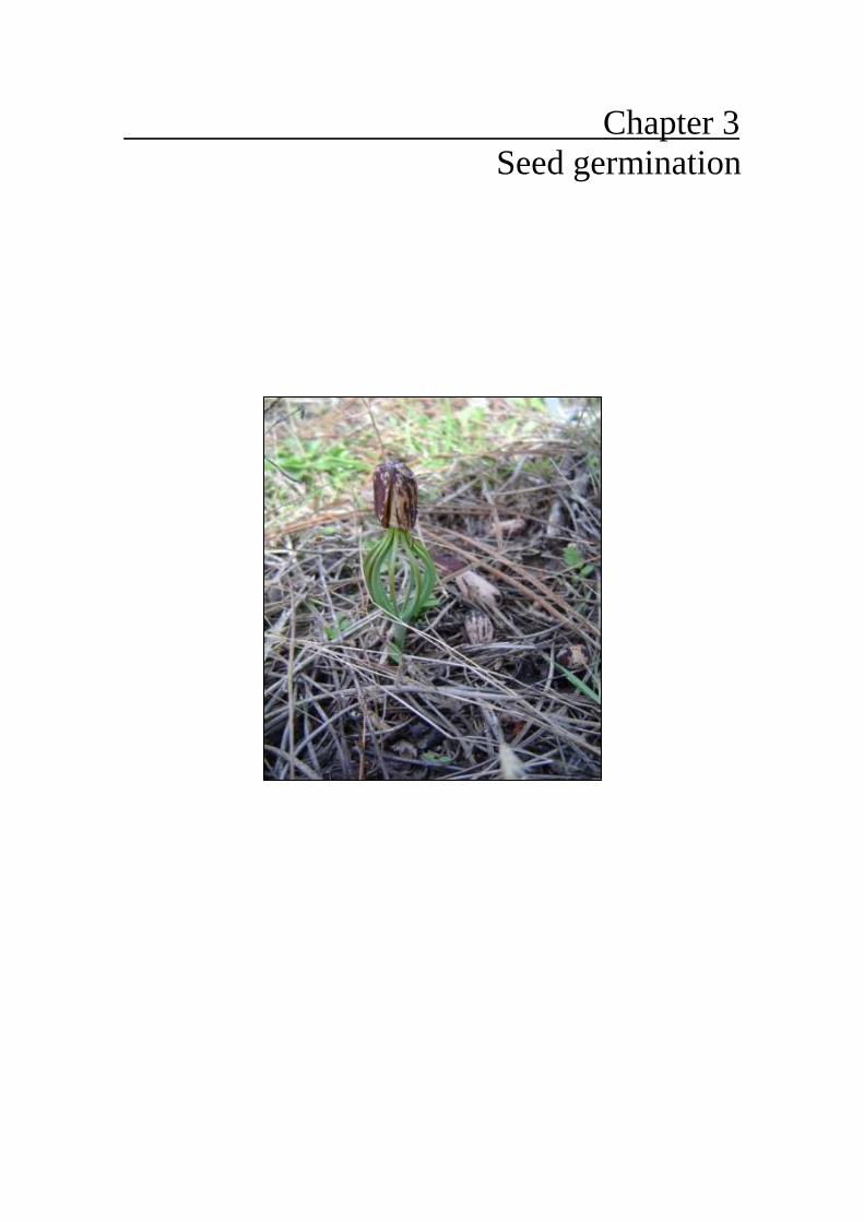
Chapter 3 Seed germination
3. Seed germination


Based on:
Manso, R., Fortin, M., Calama, R. & Pardos, M. (2012) Modelling seed germination in forest tree species through survival analysis. The Pinus pinea L. study case. Forest Ecology and Management, in press.
Specific objectives:
1. Selecting variables to include in the different submodels that are easily-accessible or
controllable by forest managers so that the final model can truly constitute a decision-
making tool
3.- Modelling the spatio-temporal transition probability of the dispersed seeds to
germinate, through the ecological factors involved in the germination subprocess
6. Identifying the potential bottlenecks that could affect natural regeneration at
subprocess level, taking into consideration the silvicultural practices and the ecological
processes involved
Data:
- Germination occurrence data series (2006-2010) from plots P3 and P4 from the natural
regeneration INIA site in La Pedraja de Portillo (Valladolid)
Methodology:
- Proportional-hazards mixed model
Main findings:
- Seed germination is mainly a climate-mediated processes, strongly hampered by frost
occurrence and temperatures out of a narrow optimal range
- The absence of overstory negatively affects germination. Also, a time-lag in the
response was detected
- Proportional-hazards models with no assumptions in the definition of the baseline
represent an interesting tool for modelling seed germination in forest tree species
Management implications:
- Germination may constitute a bottleneck for regeneration, given the high incertitude of
the process as a consequence of the narrow window of adequate conditions
- The strict scheduling of current regeneration systems neglect this aspect and,
consequently, more flexible felling schemes should be applied

––––––––––––––––––––––––––––––––––––––––––––– Chapter 3: Seed germination
57
3. Seed germination
3.1. Abstract
The direct application of existing models for seed germination may often be
inadequate in the context of ecology and forestry germination experiments. This is
because basic model assumptions are violated and variables available to forest managers
are rarely used. In this paper, we present a method which addresses the aforementioned
shortcomings. The approach is illustrated through the case study of Pinus pinea L. Our
findings will also shed light on the role of germination in the general failure of natural
regeneration in managed forests of this species. The presented technique consists of a
regression mixed model based on survival analysis. Climate and stand covariates were
tested. Data for fitting the model were gathered from a 5-year germination experiment
in a mature, managed P. pinea stand in the Northern Plateau of Spain in which two
different stand densities can be found. The model predictions proved to be unbiased and
highly accurate when compared with the training data. Germination in P. pinea was
controlled through thermal variables at stand level. At microsite level, low densities
negatively affected the probability of germination. A time-lag in the response was also
detected. Overall, the proposed technique provides a reliable alternative to germination
modelling in ecology/forestry studies by using accessible/suitable variables. The P.
pinea case study highlights the importance of producing unbiased predictions. In this
species, the occurrence and timing of germination suggest a very different regeneration
strategy from that understood by forest managers until now, which may explain the high
failure rate of natural regeneration in managed stands. In addition, these findings
provide valuable information for the management of P. pinea under climate-change
conditions.
Keywords: Survival analysis, hazard function, random effects, natural regeneration,
climate change, dormancy

––––––––––––––––––––––––––––––––––––––––––––– Chapter 3: Seed germination
58
3.2. Introduction
Natural regeneration is a key process in plant population dynamics consisting of
several well-defined stages such as dispersal, predation, germination and establishment
(Gómez-Aparicio, 2008). Germination occurrence and germination timing play an
essential role in subsequent seedling emergence (Baskin and Baskin, 2001) and
therefore, in the overall success of natural regeneration. Hence, the development of
tools to predict germination events will lead to an improvement in our understanding of
regeneration dynamics, which is a major issue in sensitive ecosystems affected by
global change or where natural disturbances have been substituted by management
(Dullinger et al., 2004; Castro et al., 2005; Brudvig and Asbjiornsen, 2009).
Germination modelling has been developed extensively within an agronomic
framework, mainly through the hydrothermal model (Gummerson, 1986; Bradford,
1990), which is a nonlinear regression approach based on the cumulative effect of water
potential and temperature on the cumulative germination rate. However, these methods
have been reported to be limited when the true germination time is unknown (Onofri et
al., 2010). This is the case in experiments that are revisited at specific intervals (Rees
and Long, 1993) or where seeds do not germinate before the end of the experiment
(Scott and Jones, 1990). Therefore, rather than the exact moment of germination, the
observation data situates the time of germination either within a given interval (interval
censoring) or at an undetermined moment after the last measurement (right censoring).
Not considering the data as censored in these cases (e.g. hydrothermal model) leads to
misspecifications of the likelihood function, which results in biased parameter estimates
(Onofri et al., 2010).
Another constraint of the hydrothermal model in studies concerned with
predicting germination under natural conditions is the type of covariate used. In
practice, water potential is difficult to obtain, hence it is not feasible to make predictions
based on this data type at stand, forest or regional scale. However, there are a number of
other variables closely associated with water availability which are more readily
available and which can be used instead. Soil water content, in particular, can be
expressed as a function of time since the last significant rainfall (Roman et al., 2000),
depending on the water-holding capacity of the soil. The relative humidity of the air
influences water loss through evapotranspiration (Müller, 2000). Additionally, when

––––––––––––––––––––––––––––––––––––––––––––– Chapter 3: Seed germination
59
attempting to identify the thermal requirements for germination under natural
conditions, frost occurrence should be taken into account together with temperature.
Although low temperatures can induce changes in a hypothetical dormancy state
(Baskin and Baskin, 2001), little is known about the effect of frosts on the instantaneous
capacity to germinate. In addition, stand structure and density can modify the general
climatic conditions at microsite scale (Keyes et al., 2009) as well as limit the possible
influence of light as a germination enhancing factor (Seiwa et al., 2009). However,
stand-related variables are commonly overlooked in existing germination models.
Germination modelling based on survival time analyses was suggested as an
option to cope with censoring in the 1980s (Scott et al., 1984; Pyke and Thompson,
1986). The first applications arose about 10 years afterwards. Rees and Long (1993)
developed a likelihood function for interval censoring in order to analyse cohorts of
emerged plants at year level. Right censoring was, however, the main concern where
data were collected at short enough intervals that made interval censoring negligible
(Fox et al., 1995; Evans et al., 1996). Although there are some other subsequent
examples of this approach for germination, new improvements have only recently been
developed, for instance, to include corrections for seeds that acquire dormancy (Onofri
et al., 2011). However, all these models relied on the assumption that time to
germination follows a specific distribution, which leads to a time-dependent underlying
process for germination (also referred as to “baseline”). Additionally, as these
experiments were not designed within a forestry framework, the correspondent models
usually neglect to test stand and/or other easily measurable variables, just as in the case
of the hydrothermal approach.
Two main families of regression models which include survival time analysis
have been commonly used: Accelerated Failure Time (AFT) models and proportional
hazard (PH) models (Lawless, 2003). These two types differ in the way that the
covariates enter the model. Whereas in AFT models the covariates modify the survival
response by altering the time scale, PH models include a fixed survival response (or
“baseline”) as a function of time, which is affected by a function of covariates. In the
present study, a PH model is developed in order to achieve a clearer understanding and
more precise prediction of seed germination in forest tree species under natural
conditions.
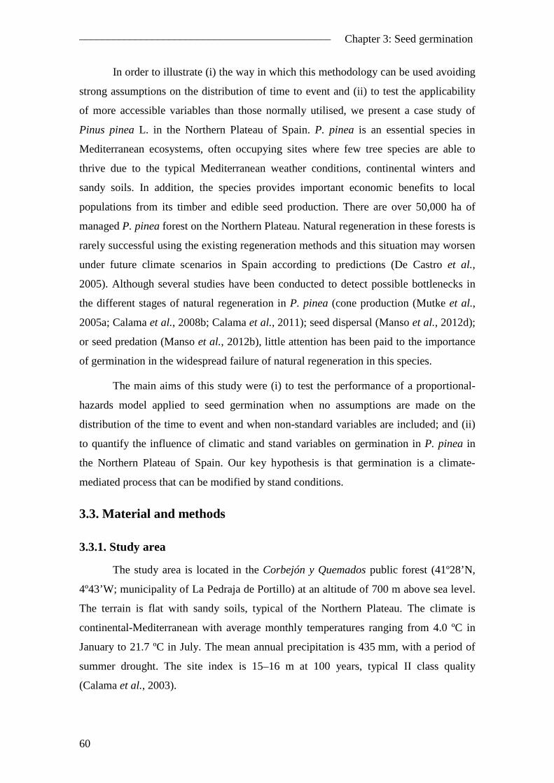
––––––––––––––––––––––––––––––––––––––––––––– Chapter 3: Seed germination
60
In order to illustrate (i) the way in which this methodology can be used avoiding
strong assumptions on the distribution of time to event and (ii) to test the applicability
of more accessible variables than those normally utilised, we present a case study of
Pinus pinea L. in the Northern Plateau of Spain. P. pinea is an essential species in
Mediterranean ecosystems, often occupying sites where few tree species are able to
thrive due to the typical Mediterranean weather conditions, continental winters and
sandy soils. In addition, the species provides important economic benefits to local
populations from its timber and edible seed production. There are over 50,000 ha of
managed P. pinea forest on the Northern Plateau. Natural regeneration in these forests is
rarely successful using the existing regeneration methods and this situation may worsen
under future climate scenarios in Spain according to predictions (De Castro et al.,
2005). Although several studies have been conducted to detect possible bottlenecks in
the different stages of natural regeneration in P. pinea (cone production (Mutke et al.,
2005a; Calama et al., 2008b; Calama et al., 2011); seed dispersal (Manso et al., 2012d);
or seed predation (Manso et al., 2012b), little attention has been paid to the importance
of germination in the widespread failure of natural regeneration in this species.
The main aims of this study were (i) to test the performance of a proportional-
hazards model applied to seed germination when no assumptions are made on the
distribution of the time to event and when non-standard variables are included; and (ii)
to quantify the influence of climatic and stand variables on germination in P. pinea in
the Northern Plateau of Spain. Our key hypothesis is that germination is a climate-
mediated process that can be modified by stand conditions.
3.3. Material and methods
3.3.1. Study area
The study area is located in the Corbejón y Quemados public forest (41º28’N,
4º43’W; municipality of La Pedraja de Portillo) at an altitude of 700 m above sea level.
The terrain is flat with sandy soils, typical of the Northern Plateau. The climate is
continental-Mediterranean with average monthly temperatures ranging from 4.0 ºC in
January to 21.7 ºC in July. The mean annual precipitation is 435 mm, with a period of
summer drought. The site index is 15–16 m at 100 years, typical II class quality
(Calama et al., 2003).
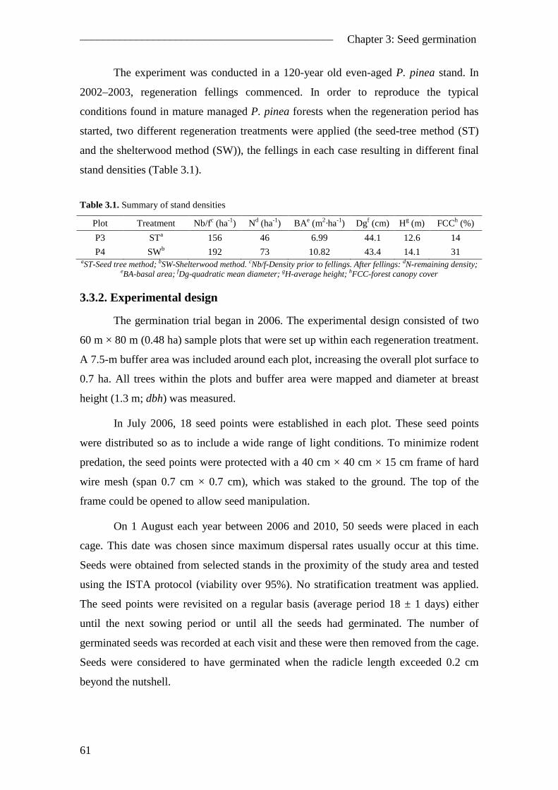
––––––––––––––––––––––––––––––––––––––––––––– Chapter 3: Seed germination
61
The experiment was conducted in a 120-year old even-aged P. pinea stand. In
2002–2003, regeneration fellings commenced. In order to reproduce the typical
conditions found in mature managed P. pinea forests when the regeneration period has
started, two different regeneration treatments were applied (the seed-tree method (ST)
and the shelterwood method (SW)), the fellings in each case resulting in different final
stand densities (Table 3.1).
Table 3.1. Summary of stand densities
Plot Treatment Nb/fc (ha-1) Nd (ha-1) BAe (m2·ha-1) Dgf (cm) Hg (m) FCCh (%)
P3 STa 156 46 6.99 44.1 12.6 14
P4 SWb 192 73 10.82 43.4 14.1 31 aST-Seed tree method; bSW-Shelterwood method. cNb/f-Density prior to fellings. After fellings: dN-remaining density;
eBA-basal area; fDg-quadratic mean diameter; gH-average height; hFCC-forest canopy cover
3.3.2. Experimental design
The germination trial began in 2006. The experimental design consisted of two
60 m × 80 m (0.48 ha) sample plots that were set up within each regeneration treatment.
A 7.5-m buffer area was included around each plot, increasing the overall plot surface to
0.7 ha. All trees within the plots and buffer area were mapped and diameter at breast
height (1.3 m; dbh) was measured.
In July 2006, 18 seed points were established in each plot. These seed points
were distributed so as to include a wide range of light conditions. To minimize rodent
predation, the seed points were protected with a 40 cm × 40 cm × 15 cm frame of hard
wire mesh (span 0.7 cm × 0.7 cm), which was staked to the ground. The top of the
frame could be opened to allow seed manipulation.
On 1 August each year between 2006 and 2010, 50 seeds were placed in each
cage. This date was chosen since maximum dispersal rates usually occur at this time.
Seeds were obtained from selected stands in the proximity of the study area and tested
using the ISTA protocol (viability over 95%). No stratification treatment was applied.
The seed points were revisited on a regular basis (average period 18 ± 1 days) either
until the next sowing period or until all the seeds had germinated. The number of
germinated seeds was recorded at each visit and these were then removed from the cage.
Seeds were considered to have germinated when the radicle length exceeded 0.2 cm
beyond the nutshell.
––––––––––––––––––––––––––––––––––––––––––––– Chapter 3: Seed germination
62
In addition to germination measurements, daily climatic variables, such as the
mean, maximum and minimum temperatures, mean relative humidity (ratio of the
partial pressure of water vapour in the air to the saturated vapour pressure of water),
daily precipitation, days with precipitation and days with frost were gathered from a
nearby meteorological station (41º17'N, 4º40'W; data available in www.inforiego.org).
To estimate light availability at each seed point, Global Site Factor (GSF) was
calculated from hemispheric photographs taken at each cage. GSF is the proportion of
global solar radiation (direct plus diffuse) under a plant canopy relative to that in the
open. The resulting index was corrected for the angle of incidence relative to a flat
intercepting surface. The water-holding capacity of the surface layer of the soil was
obtained for each point through texture analysis of two soil samples taken near to each
seed point, following the method by Gandullo (1985). Each sample comprised the top
20 cm of the soil profile (soil cylinder of 1.57 dm3).
Finally, in order to take into account the possible influence of trees on
microclimate conditions at ground level, we calculated the influence potential (IPOT) of
all trees located within a 15 m radius of each seed point. None of the seed points were
located at distance below 15 m from the outside margin of the buffered area. IPOT is a
competition index based on the concept of ecological field theory (Wu et al., 1985) and
empirically modified by Kuuluvainen and Pukkala (1989) and Barbeito et al. (2011):
IPOTj = 1 – GPOTj
where ( )∏=
−=jn
hhjj IGPOT
1
1 and Ihj = Ihj(0) × exp(– b·dhj)
Ihj is the potential influence of tree h at seed point j, dhj is the distance from tree
h to seed point j, Ihj(0) is dbhhj/(max dbhh at each plot), dbhhj is the diameter at breast
height of tree h in the influence area of seed point j, b is a parameter, and nj is the
number of trees in the influence area of seed point j. A value of 0.25 was heuristically
assigned for b. IPOT ranges from zero (no competition) to one (maximum competition).
The range of all variables, along with observed seasonal cumulative germination
rates are shown in Table 3.2.

––––––––––––––––––––––––––––––––––––––––––––– Chapter 3: Seed germination
63
3.3.3. Survival analysis
Germination modelling was approached through survival analysis. To illustrate
the basis of this technique, let T be defined as a random variable that corresponds to the
time until germination for a particular seed. The cumulative density probability of T at
time t is actually the probability that germination occurred at or before time t, i.e. F(t) =
P(T ≤ t). The survival function S(t) is the probability that a particular seed remains latent
after time t, i.e. S(t) = 1 – F(t). The hazard function h(t) represents the instantaneous
germination rate, or hazard for a given seed at time t, providing it is still latent at time t.
This hazard function is related to the survival function as follows:
( )
−= ∫
tdxxhtS
0)(exp [3.1]
The survival function (equation [3.1]) implies that the probability of a seed
remaining latent at time t is a decreasing function of the sum of all hazards prior to time
t.
Table 3.2. Summary of variables of interest and observed values for seasonal cumulative germination for
the 5 years of study
mean max min stand. error
spatial covariates
WHCa (mm/cm depth of soil) 104.2267 141.7141 84.0367 2.2125
GSFb 0.6654 0.8629 0.4163 0.0169
IPOTc 0.4031 0.7174 0.1492 0.0272
time-varying covariates
mean temperature (°C) 11.43 28.03 – 5.19 0.15
maximum temperature (°C) 18.36 38.5 – 1.71 0.19
minimum temperature (°C) 4.41 19.59 – 12.02 0.13
relative humidity (%) 67.14 100 17.83 0.37
freezing days year-1 90.4 114 74 8.18
rainfall days year-1 128.6 161 90 12.20 cumulative germination (%)
Fall Winter Spring 2006-2007 89.74 90.92 - 2007-2008 9.63 22.81 43.35 2008-2009 4.31 7.04 8.3 2009-2010 55.04 63.82 79.61 2010-2011 60.94 65.12 71.13
aWHC-water holding capacity; bGSF-Global Site Factor; cIPOT-overstory influence potential

––––––––––––––––––––––––––––––––––––––––––––– Chapter 3: Seed germination
64
3.3.4. Hazard function definition
The hazard function includes time-varying and time-independent explanatory
variables as well as a number of unknown parameters. Covariates tested in this study
were of three types: (i) thermal variables (days elapsed from the last frost event (fr) and,
alternately, daily mean, maximum and minimum temperature (temp) in ºC); (ii) water
availability-related variables (water-holding capacity (WHC), daily relative air humidity
(rh), daily precipitation (dp) and days elapsed from the last precipitation event (prec));
and (iii) stand-related variables: Global Site Factor (GSF) and IPOT.
For the sake of clarity, let i, j, k, l and m be the indices of the plot, the seed point,
the year, the seed and the day, respectively. In order to take into account the time-
varying covariates, the hazard function can be expressed on a daily basis, i.e.
( )
−= ∑=
t
mijklmijkl htS
1
),(exp βx [3.2]
where t is the number of days since seed l at seed point j in plot i was sown on 1 August
of year k; xijklm is a vector of explanatory variables, some of which are measured daily;
and β is a vector of unknown but estimable parameters.
From a biological perspective, we can infer that the response of the germination
to various explanatory variables is not linear, but rather, nonlinear with some optimal
values. Consequently, it can be assumed that the hazard is the product of nonlinear
functions of the explanatory variables such that
( ) ( ) ( )( ) ( ) ( ) ( ) ( )( )91,988776655
443322110
,,,,,
),(,,,),(
βxββββ
ββββββx
−+⋅⋅⋅
⋅⋅⋅⋅⋅=
mijklkmkmkmkm
kmijijijijklm
hftempffrfprecfdpf
rhfWHCfGSFfIPOTfh [3.3]
where β = (β0T,β1
T,β2T,β3
T,β4T,β5
T,β6T,β7
T,β8T,β9
T)T.
The functions f1–f8 define the effect of each explanatory variable on the daily
probability of germination. The independent multiplicative parameter β0 is a sort of
scaling factor that can be understood as a generic model baseline. The function
f9(h(xijkl,m-1, β9)) = β9h(xijkl,m-1) acts like a lag in the response. In other words, the current
daily probability of germination is expected to depend also on the conditions of
previous days. In statistical terminology, this lag function is similar to an autoregressive
correlation structure (Pinheiro and Bates, 2000, ch. 5.3).

––––––––––––––––––––––––––––––––––––––––––––– Chapter 3: Seed germination
65
We defined the functions f1–f8 so that they range from 0 (maximum hazard
reduction) to 1 (minimum hazard reduction). Negative values would be inconsistent as
they would lead to a survival function Sijkl(t) that could exceed 1. In such a context, the
product of the functions f1–f8 seemed to be a desirable feature because we expected the
effect of the explanatory variables to be multiplicative. Also, from a biological
standpoint, this form made more sense as unfavourable conditions from one explanatory
variable are likely to reduce the hazard to zero for a particular day if we put aside the
lag effect. Therefore, our hazard function can be seen as a product of ecological factors
that can reduce the maximum daily germination hazard represented by β0. The challenge
remained to find a functional form that made sense for each function.
Provided that the potential lowest value for IPOTij, GSFij, WHCij, rhkm and dpkm
is zero and that it can be assumed that their influence on germination increases with the
value of the explanatory variable, the corresponding functions can be parameterized as:
f1(IPOTij,β1) = 1 – exp(β1IPOTij)
f2(GSFij,β2) = 1 – exp(β2GSFij)
f3(WHC,β3) = 1 – exp(β3WHCij)
f4(rhkm,β4) = 1 – exp(β4rhkm)
f5(dpkm,β5) = 1 – exp(β5dpkm)
where the parameters can only adopt negative values.
In the case of rainfall and frost events, we assumed that these have long lasting
effects on the hazard. We hypothesised that germination hazard was intensified when a
precipitation event takes place, the effect decreasing with the number of days since
precipitation occurrence. As preckm equals zero on the day of precipitation occurrence,
the corresponding function can be defined as f6(preckm,β6) = exp(β6preckm), with β6<0.
Inversely, freezing was thought to reduce hazard as a function of the number of days
elapsed since the last frost, with maximum reduction taking place on days when frost
occurred( )0=kmfr . Hence it can be parameterized as f7(frkm,β7) = 1 – exp(β7frkm), where
β7<0.
Finally, the response to the temperature effect was defined as a non-negative
function with a maximum in accordance with existing knowledge on seed ecology
(Bewley and Black, 1994). Daily mean, maximum and minimum temperatures were

––––––––––––––––––––––––––––––––––––––––––––– Chapter 3: Seed germination
66
tested under different parameterizations based on those summarized by Kamkar et al.
(2012) plus an additional logistic option. We also considered a strictly non-skewed
function through a scaled Normal probability density function that ranged from 0 to 1
(Table 3.3).
Table 3.3. Temperature functions tested
Function Equation
( )
( )
( )
( )( ) ( )( )
( )( )( )( )
( ) ( )
( ) ( )
−−=
−−=
>+=≤+=
−−×
−−=
≥≤=
<≤−−−=
<<−
−=
−−
2
2
8
1221
228
118
max
max8
max8
maxmax
8
8
2exp Normal Scaled
where
logit
logitLogistic
Beta
0
1Segmented
σµ
λληηµ
µληµλη
µµµ
µµµ
µµ
µµµµµ
µµµµ
µ
µµµµ
okmkm
o
okmkmkm
okmkmkm
o
km
bo
bkmkm
kmbkmkm
kmoo
okmkm
okmbbo
bkmkm
temptempf
tempiftemptempf
tempiftemptempf
temptemptempf
temportempiftempf
tempiftemp
tempf
tempiftemp
tempf
aboom
The Segmented and Beta functions comprise the following parameters defining the appropriate thermal interval for germination: µo (optimum temperature), µb (base temperature) and µmax (ceiling temperature). The logistic function
includes intercept (η1-2) and slope (λ1-2) from where µo can be deduced. Parameters in the scaled Normal function are µo and σ, the latter accounting for the amplitude of the thermal interval. tempkm stands for temperature at plot k in
day m
3.3.5. Likelihood function formulation
The data presented in this study are actually interval censored seed lifetimes
since observations were carried out periodically. As a consequence, the exact moment
of germination is unknown. For each seed l in year k at seed point j in plot i, we only
know that the germination time Tijkl took place within an interval of time where the
upper bound is the observation confirming seed germination and the lower bound is the
previous observation when the seed had not yet germinated. In other words, we know
that tlower,ijkl <Tijkl <tupper,ijkl where tlower,ijkl and tupper,ijkl represent the two limits of the time
interval. If the seed fails to germinate during year k, then tupper,ijkl = ∞ and Tijkl is said to
be right-censored.

––––––––––––––––––––––––––––––––––––––––––––– Chapter 3: Seed germination
67
Therefore, the marginal likelihood function for this experiment is
( ) ( )[ ] ( )[ ] ijklijkl qijkllowerijkl
q
i j k lijkllowerijklijklupperijkl tStStS −⋅−= ∏∏∏∏ 1
,,,l [3.4]
where Sijkl(t) is the survival function that sums the daily hazards h(xijklm,β) (equation
[3.3]) in the terms shown in equation [3.2] and qijkl is a dummy variable that equals one
when the seed has germinated during a known interval (tupper,ijkl–tlower,ijkl] and zero if it is
right-censored in relation to this interval.
3.3.6. Model fitting and evaluation
In addition to the explanatory variables, we also tried to account for the data
structure. In fact, the sampling scheme is likely to result in clustered data and the
correlation between observations that belong to the same plot i, seed point j, and/or year
k of study might be non-null. In order to prevent this violation of the independence
assumption, a vector b of random effects ui, vj and wk for the mentioned levels of
variability was included through the expansion of parameter β0, the generic baseline.
Random effects are assumed to be normally distributed so that b~N(0, D), where D is
the random effects variance–covariance matrix. Although random effects are commonly
included as a multiplicative parameter and they are assumed to follow a distribution
adopting non-negative values only (i.e. Gamma; Lawless (2003, p. 497)), computing
limitations to accommodate our customized hazard function with correction for data
correlation forced us to use the present formulation. Also severe problems of
convergence arise when different levels of variability are simultaneously considered,
especially if it implies crossed effects. Therefore, random effects were tested separately
and the resulting models were evaluated in terms of Akaike Information Criteria (AIC).
In order to illustrate the effect of each explanatory variable and optimal
conditions for germination, the marginal hazard function was plotted against the
covariate of interest whereas the rest was set to its theoretical maximum. Where
possible, a comparison with average climatic conditions in the area was performed.
IPOT influence on germination needs to be interpreted in terms of density. Therefore,
IPOT was simulated in the central 70 m × 70 m subplot of a 100 m × 100 m plot at a
scale of 1 m2 for different stocking densities, considering regular spacing and identical
diameters for all trees. The IPOT effect, where significant, was then computed based on
the resulting model parameterization for each simulated plot.

––––––––––––––––––––––––––––––––––––––––––––– Chapter 3: Seed germination
68
The model accuracy was evaluated using graphical methods on the training data.
Conditional predictions of cumulative germination proportion (F(t) = 1 – S(t)) were
averaged for each interval across all seed points and compared with the corresponding
observed values for those intervals. This approach provides evidence of the existence of
bias (systematic error in the prediction of the mean) and shows in a simple manner the
degree of agreement between model and data (overall agreement between the predicted
and observed pattern of germination). Additionally, bias was quantified through the
mean error (E) of F(t) for all n individual observations:
( ) ( )( )n
tFtFE ijkl ijklijkl∑ −
=ˆ
[3.5]
All calculations were carried out using PROC NLMIXED in SAS 9.2.
3.4. Results
3.4.1. Hazard function
Optimisation of the likelihood function shown in equation [3.4] was not
straightforwardly achieved under the proposed parameterization. In the selection
process we found most of the combinations of parameters to result in severe problems
of convergence. This is particularly true in all cases where dpkm and/or rhkm were
included in the model. When the model was fitted without the aforementioned
covariates, convergence was achieved either if GSFij and WHCij or, alternately, prepkm
were excluded from model formulation. When fitting the model considering the first
possibility, prepkm was the only non-significant covariate (p-value 0.2327). In regard to
the second possibility, both GSFij and WHCij were also found to be non-significant (p-
values 0.9315 and 0.9877, respectively) and consequently the model was alternately
fitted with each of them at a time. In this process, WHCij was found to be non-
significant, whereas convergence was not attained when the model included GSFij. As it
can be seen, both possibilities led to the same set of parameters when non-significant
covariates are dropped of the model. Therefore, germination hazard was finally defined
by the overstory competition (IPOTij), number of days elapsed from last frost event
(frkm) and daily temperature (tempkm), all of them significant. These variables modulated
the generic base germination through interaction with the baseline (parameter β0; p-
value<0.0106). The autoregressive term was also found to be significant. Out of all the

––––––––––––––––––––––––––––––––––––––––––––– Chapter 3: Seed germination
69
mentioned options for the temperature effect (Table 3.3), only the scaled Normal
approach proved adequate, as the rest implied poorly-resolved estimates with large
values in the gradient matrix. Maximum daily temperature produced the best fits and
was therefore used in preference to mean and minimum temperature. Selected fixed
effects were similar irrespective of the variance structure tested. As regards the random
effects, year level of variability performed better (AIC 24,821) than seed point (AIC
24,861) or plot (AIC 25,218). The AIC value for the marginal model was 25,242, which
indicates a better performance when random effects are included. Table 3.4 presents the
parameter estimates of the preferred model.
In order to assure we did not have problems of collinearity among the spatial
covariates that could yield an incorrect variable selection, the final model was
additionally fitted excluding IPOTij and alternately testing GSFij and WHCij. As a result,
convergence problems identically arose when GSFij was considered in absence of
WHCij, whereas the latter was non-significant (p-value 0.9820).
Table 3.4. Summary of parameter estimates for the selected model
parameter estimate std. error df t value p-value
β0a 0.0250 0.0057 4 4.53 0.0106
β1b – 8.4053 0.7211 4 – 11.66 0.0003
β7c – 0.0127 0.0016 4 – 7.94 0.0014
µod 14.1700 0.0537 4 263.76 <0.0001
σ2e 0.7486 0.0244 4 30.73 <0.0001
β8f 0.9603 0.0023 4 421.8 <0.0001
σ2wk
g 0.0001 - - - - aβ0: generic baseline; bβ1 and cβ7: parameters related to IPOT and frost occurrence, respectively; dµo: optimum daily
maximum temperature; eσ2: variance of the (scaled) normally distributed germination response to maximum temperature; fβ8: autoregressive parameter; gσ2
wk : variance linked to year random effect
3.4.2. Optimum conditions for germination
The parameterized hazard function produces a hyperplane, depending on
climatic and environmental variables, from which a set of the most favourable
conditions can be deduced. Optimum daily maximum temperature was found to be 14.2
ºC, the value of parameter µ0, and the symmetric thermal interval ranges from 12 to 16
ºC approximately (Fig. 3.1a). The hazard-reducing effect of frost occurrence only
became negligible after 300 days from the frost event, whereas germination risk is set to
zero on days when freezing occurs (Fig. 3.1b). As regards IPOT, only very low values
for this variable notably reduced germination risk (when IPOT equals 0.3, hazard
––––––––––––––––––––––––––––––––––––––––––––– Chapter 3: Seed germination
70
reduction with respect to the maximum is only 10.5%). Fig. 3.2 shows that densities
over 25 stems·ha-1 resulted in a reduction in germination of up to 20% in simulated
plots, which implies that only where the overstory is very sparse is there any notable
conditioning of germination. Theoretically, germination hazard will be null when
overstory competition completely disappears (Fig. 3.1c). Finally, the autoregressive
term showed a notable influence, for example, considerably mitigating the effect of frost
(Fig. 3.1d). In addition, the autoregressive factor causes the hazard value to increase
beyond its theoretical maximum when suitable conditions for germination occur (Fig.
3.1e).
When considering historic climatic records, Fig. 3.3 shows how temperatures
between June and September over the last 10 years were higher in general than those
suitable for germination. In winter, the effect of frost cancels out the potential hazard
increase, even if adequate thermal conditions are possible (December and January).
Figure 3.1. Marginal effects on hazard of the different covariates included in the model (solid line). (a-
c) Daily maximum temperature (temp), frost occurrence (fr), IPOT. The rest of fixed effects were set to
one and autoregressive term not consider. (d-e) Autoregressive parameter over time (maximum initial
hazard) during 10 consecutive freezing days and during 10 consecutive days of optimum temperature

––––––––––––––––––––––––––––––––––––––––––––– Chapter 3: Seed germination
71
Figure 3.3. Histograms of maximum (white) and minimum (light grey) daily temperatures. Dark grey
area represents theoretical suitable thermal interval for germination. Vertical dashed line highlights
freezing value (0 ºC)
Figure 3.2. Histograms of IPOT values and corresponding reducing effects on hazard for three different
densities. Evaluation was carried out in a simulated 70 m × 70 m plot at 1 m2 scale
––––––––––––––––––––––––––––––––––––––––––––– Chapter 3: Seed germination
72
Given that frost presents a highly durable effect, spring germination is unlikely
in the area and restricted to years with unusually warm winters, such as that of 2007–
2008. It can be deduced, therefore, that the optimum germination period in the Northern
Plateau are the months of October and November, when there is a greater probability of
favourable conditions and the possible influence of frost is less likely.
3.4.3. Model evaluation
Predictions of the proportion of germinated seeds over time closely mimic the
observed patterns in the two sample plots for all the years of the study (Fig. 3.4). The
model proved to be highly accurate for all years, although displaying a slightly weaker
performance in 2009–2010. Furthermore, no bias pattern was apparent, which is
confirmed by the low absolute value of the mean error (E = – 0.0166).
3.5. Discussion
3.5.1. Modelling approach
Although survival analysis techniques have been scarcely used in the context of
seed germination compared to other methodologies, the recent comparative studies
carried out by Onofri et al. (2010) and Onofri et al. (2011) demostrate the superiority of
Figure 3.4. Predicted (solid line) and observed (crossed-solid line) cumulative proportion of germinated
seeds. The abscissa is a one year temporal axis starting at the seed deployment date
––––––––––––––––––––––––––––––––––––––––––––– Chapter 3: Seed germination
73
those models developed through survival analysis. The present paper confirms the
potential of survival analysis applied to germination when censored observations are
present. We also demonstrate that conventional formulations can be successfully
adapted to avoid strong assumptions on the baseline of the process and to include non-
standard explanatory variables. Furthermore, the proposed model extends the existing
methods to fulfil further model assumptions, such as independence of observations
through random effects. Although the use of mixed effect modelling is unavoidable
when the independence assumption is violated, it has been scarcely employed in the
context of survival analysis (but see Rose et al., 2006; Fortin et al., 2008). In our case,
we allowed our generic baseline to vary randomly among years, thus absorbing
unnoticed aggregate climatic influences on germination.
A common procedure in survival analysis is to assume a prior behaviour of the
process in question (baseline). This prior behaviour can be modified as a function of
several covariates. For instance, Onofri et al. (2010) used an AFT model to predict seed
germination based on a logistic baseline using water potential as an explanatory
variable. However, under non-controlled field conditions, there is no evidence of an
existing independent baseline for germination. In our model, we defined the
germination hazard as a function of ecological factors with no prior assumptions as
regards a baseline for seed germination, with the exception of a technically required
scaling parameter.
In the present study we also show that germination can be accurately explained
by climatic and stand covariates, at least in this particular case study. The proposed
model gained applicability through the set of selected variables in two ways: firstly,
they are readily available (as long as daily records are kept) and, secondly, they take
into account the effects of forest structure and management on microclimatic conditions
(stand variables). The inclusion of time-dependent variables allows predictions to be
generated with varying field conditions. Although this paper focuses on the case of P.
pinea, these possibilities can be explored for most tree species. As a shortcoming, it
should be noted that the use of IPOT as a stand variable could produce non-comparable
results if applied to stands with very different structures.
In contrast to the majority of germination studies, the covariates relating to water
availability proved non-significant or convergence was not achieved when included.
Concerning water-holding capacity, the notable homogeneity of the variable throughout

––––––––––––––––––––––––––––––––––––––––––––– Chapter 3: Seed germination
74
the two sampled plots could be behind this lack of significance. In regard to
precipitation, the low values for water-holding capacity would imply high drainage
coefficients (Müller, 2000) and, consequently, little impact of the covariate on water
potential reduction. With respect to relative air humidity, it is known to be highly
collinear to temperature, which in turn already determines water loss through
evapotranspiration (Müller, 2000). Given the high ecological homogeneity of this
region, it is presumable that these results would have not notably differed should we
have had a replicated design throughout the Northern Plateau. Nevertheless, it is
important to note that the non-significance of our water ability-related variables does
not necessarily mean that water potential is irrelevant: it only implies that these
covariates, under these conditions, could not capture water potential variability and that
the importance of water potential in this context is reduced in contrast to the influence
of thermal variables.
Dormancy is a major concern in seed ecology research (Chambers et al., 1999;
Baskin and Baskin, 2001). In the case study presented here it was not possible to test
dormancy processes, since the seed lots were exposed to natural conditions for a
maximum of one year. Non-germinated P. pinea seeds are assumed to perish in the
course of a year due to the high rodent predation rates occurring in the area (Manso et
al., 2012b). Under these conditions, distinction between non-germinated seeds and true
dormant seeds (if any) is not feasible. However, the proposed methodology allows us to
take into account the abovementioned phenomenon in dormancy related experiments.
The variables currently included in the model are common for interval and right
censored observations, meaning that non-germinated seeds result from an absence of
suitable enhancing factors. In order to take into account potentially dormant seeds, the
non-germinated fraction should be partitioned into those seeds that simply never
abandoned latency and those that acquired dormancy. The latter can be related to a set
of covariates z thought to induce the process through the function π(z), representing the
probability of not germinating due to dormancy. Therefore, the likelihood function in
equation [3.4] can be extended as:
( )( ) ( ) ( )( )[ ]( ) ( )( ) ( )[ ] ijkl
ijkl
qijkllowerijklijklijkl
q
i j k lijkllowerijklijklupperijklijkl
tSzz
tStSz
−⋅−+
×−⋅−= ∏∏∏∏1
,
,,
1
1
ππ
πl
[3.5]

––––––––––––––––––––––––––––––––––––––––––––– Chapter 3: Seed germination
75
similar to those used in zero-inflated model fits (Affleck, 2006; Fortin and DeBlois,
2007; Calama et al., 2011), in this case, a zero-inflated binomial distribution (Tyre et
al., 2003). A comparable approach accounting only for the dormant fraction as right
censored observations can be found in Onofri et al. (2011), as an extension of an AFT
model.
3.5.2. Pinus pinea case study
The proposed model succeeded in determining the importance of germination in
P. pinea natural regeneration in our sample plots, providing some prior outcomes about
regeneration dynamics in the species. The results of this study seem to confirm our key
hypothesis of climatic control for seed germination and the importance of forest
structure in the process.
The extrapolation of our findings to P. pinea stands in the Northern Plateau as a
whole must be made prudently, as we did not have a randomized design over the region.
However, the high homogeneity of conditions throughout the area leads us to suggest
that the role of germination in the P. pinea regeneration strategy could be described as
follows: P. pinea seed dispersal takes place from June to early November (Manso et al.,
2012d), whereas maximum rates of seed predation occur in winter months (Manso et
al., 2012b) due to higher rodent activity in Mediterranean areas outside the dry period
(Díaz et al., 2010). These circumstances lead to a seed-limiting scenario in spring,
coinciding with the scarce likelihood of germination predicted for these months. In
addition, Calama et al. (2012) found that seedlings established in the fall are more likely
to survive the following summer drought period than those produced by spring
germinated seeds. Therefore, rapid germination in fall, regardless of site characteristics,
could be a key factor for natural regeneration in P. pinea, creating a perfectly
synchronized post-fructification strategy.
However, this “window” of optimal conditions in fall is not guaranteed every
year. Therefore, such a strategy only makes sense if there is a relatively long period for
regeneration and a significant seed source density, which permits both dispersal and
germination to occur simultaneously. Consequently, a light-independent germination
pattern would be expected. Our findings suggest such a pattern (non-significant GSF),
at least in the Northern Plateau. Accordingly, Seiwa et al. (2009) stated that large-
seeded, non-pioneer species show little sensitivity to environmental signals which

––––––––––––––––––––––––––––––––––––––––––––– Chapter 3: Seed germination
76
enhance germination potential. Non-detection of light as a gap signal along with
germination reduction at very low densities leads to a seedling shadow which
potentially mimics the seed shadow (Calama et al., 2012). This fact would confirm the
medium shade-tolerant behaviour of P. pinea reported by Awada et al. (2003) and
therefore, the tendency to naturally produce uneven-aged stands (Calama et al., 2008a).
In turn, this stand structure ensures long periods for seedling emergence in the absence
of large gaps.
In contrast with the strategy described above, the currently-applied regeneration
methods in the study area assume a strong shade-intolerant behaviour in stone pine
(Montero et al., 2008). For this kind of species, intensive fellings are prescribed to
achieve natural regeneration (Smith et al., 1996). However, such practices rapidly lead
to seed limitation in P. pinea forests (Manso et al., 2012d). If efficient germination has
not occurred prior to reducing tree density, natural regeneration will obviously be
affected. Additionally, the presence of large gaps in the forest canopy is not favourable
to germination.
The future climatic scenario in Spain is characterized by increasing mean and
maximum temperatures, particularly during the warm period (De Castro et al., 2005).
Minimum temperatures in winter, however, are expected to be more stable. According
to these predictions, suitable conditions for germination in terms of daily temperature
may shift towards the colder months, but the only moderate reduction in frost
occurrence during this period implies a high degree of uncertainty in regard to the
likelihood of successful germination.
Under the present climatic conditions and management methods employed in P.
pinea stands in the Northern Plateau, germination can constitute a bottleneck for the
natural regeneration of the species. From an ecological perspective, the intensity of
regeneration treatments should be reduced and also delayed until a few years after the
occurrence of favourable germination/recruitment events in accordance with the light
requirements of the species and subsequent natural forest dynamics. In a scenario of
global climate change, predictions for future climatic conditions in the Mediterranean
basin underline the necessity to consider the recommendations outlined in this paper.

––––––––––––––––––––––––––––––––––––––––––––– Chapter 3: Seed germination
77
References
Affleck, D. L. R. (2006) Poisson mixture models for regression analysis of stand level mortality. Canadian Journal of Forest Research-Revue Canadienne De Recherche Forestiere, 36, 2994-3006.
Awada, T., Radoglou, K., Fotelli, M. N. & Constantinidou, H. I. A. (2003) Ecophysiology of seedlings of three Mediterranean pine species in contrasting light regimes. Tree Physiology, 23, 33-41.
Barbeito, I., LeMay, V., Calama, R. & Canellas, I. (2011) Regeneration of Mediterranean Pinus sylvestris under two alternative shelterwood systems within a multiscale framework. Canadian Journal of Forest Research-Revue Canadienne De Recherche Forestiere, 41, 341-351.
Baskin, C. C. & Baskin, J. M. (2001) Seeds. Ecology, biogeography, and evolution of dormancy and germination. Academic Press, San Diego.
Bewley, J. D. & Black, M. (1994) Seeds: physiology of development and germination. Plenum press, New York.
Bradford, K. (1990) A water relations analysis of seed germination rates. Plant Physiology, 94, 840-849.
Brudvig, L. & Asbjiornsen, H. (2009) Dynamics and determinants of Quercus alba seedling success following savanna encroachment and restoration. Forest Ecology and Management, 257, 876-884.
Calama, R., Barbeito, I., Pardos, M., Del Río, M. & Montero, G. (2008a) Adapting a model for even-aged Pinus pinea L. stands for complex multi-aged structures. Forest Ecology and Management, 256, 1390-1399.
Calama, R., Cañadas, N. & Montero, G. (2003) Inter-regional variability in site index models for even-aged stands of stone pine (Pinus pinea L.) in Spain. Annals of Forest Science, 60, 259-269.
Calama, R., Gordo, F. J., Mutke, S. & Montero, G. (2008b) An empirical ecological-type model for predicting stone pine (Pinus pinea L.) cone production in the Northern Plateau (Spain). Forest Ecology and Management, 255, 660-673.
Calama, R., Madrigal, G., Manso, R., Garriga, E., Gordo, F. J. & Pardos, M. (2012) Germinación, emergencia y supervivencia de regenerado en Pinus pinea L. La regeneración natural de los pinares en los arenales de la Meseta Castellana (eds J. Gordo, R. Calama, M. Pardos, F. Bravo & G. Montero). Instituto Universitario de Investigación en Gestión Forestal Sostenible (Universidad de Valladolid-INIA), Valladolid.
Calama, R., Mutke, S., Tomé, J., Gordo, J., Montero, G. & Tomé, M. (2011) Modelling spatial and temporal variability in a zero-inflated variable: The case of stone pine (Pinus pinea L.) cone production. Ecological Modelling, 222, 606-618.
Castro, J., Zamora, R., Hódar, A. & Gómez, J. (2005) Ecology of seed germination of Pinus sylvestris L. at its southern, Mediterranean distribution range. Investigaciones Agrarias: Sistemas y Recursos Forestales, 14, 143-152.
Chambers, J., Vander Wall, S. & Schupp, E. (1999) Seed and seedling ecology of piñon and juniper species in the Pygmy woodlands of Western North America. Botanical Review, 65, 1-38.
De Castro, M., Martín-Vide, J. & Alonso, S. (2005) The climate of Spain: past, present and scenarios for the 21st century. A preliminary assessment of the impacts in Spain due to the effects of climate change. ECCE Project-Final report, pp. 1-64. Ministerio de Medio Ambiente, Madrid.
––––––––––––––––––––––––––––––––––––––––––––– Chapter 3: Seed germination
78
Díaz, M., Torre, I. & Arrizabalaga, A. (2010) Relative roles of density and rainfall on the short-term regulation of Mediterranean wood mouse Apodemus sylvaticus populations. Acta Theriologica, 55, 251-260.
Dullinger, S., Dimböck, T. & Grabherr, G. (2004) Modelling climate change-driven treeline shifts: relative effects of temperature increase, dispersal and invasibility. Journal of Ecology, 92, 241-252.
Evans, A. S., Mitchell, R. J. & Cabin, R. J. (1996) Morphological side effects of using gibberellic acid to induce germination: Consequences for the study of seed dormancy. American Journal of Botany, 83, 543-549.
Fortin, M., Bedard, S., DeBlois, J. & Meunier, S. (2008) Predicting individual tree mortality in northern hardwood stands under uneven-aged management in southern Quebec, Canada. Annals of Forest Science, 65, 12.
Fortin, M. & DeBlois, J. (2007) Modeling tree recruitment with zero-inflated models: The example of hardwood stands in southern Quebec, Canada. Forest Science, 53, 529-539.
Fox, G. A., Evans, A. S. & Keefer, C. J. (1995) Phenotypic consequences of forcing germination - a general problem of intervention in experimental-design. American Journal of Botany, 82, 1264-1270.
Gandullo, J. M. (1985) Ecología Vegetal. Fundación Conde del Valle de Salazar, Madrid.
Gómez-Aparicio, L. (2008) Spatial patterns of recruitment in Mediterranean plant species: linking the fate of seeds, seedlings and saplings in heterogeneous landscapes at different scales. Journal of Ecology, 96, 1128-1140.
Gummerson, R. (1986) The effect of constant temperatures and osmotic potential on the germination of sugar beet. Journal of Experimental Botany, 37, 729-741.
Kamkar, B., Al-Alahmadi, M. J., Mahdavi-Damghani, A. & Villalobos, F. J. (2012) Quantification of the cardinal temperatures and thermal time requirement of opium poppy (Papaver somniferum L.) seeds to germinate using non-linear regression models. Industrial Crops and Products, 35, 192-198.
Keyes, C. R., Maguire, D. A. & Tappeiner, J. C. (2009) Recruitment of ponderosa pine seedlings in the Cascade Range. Forest Ecology and Management, 257, 495-501.
Kuuluvainen, T. & Pukkala, T. (1989) Effect of Scots pine seed trees on the density of ground vegetation and tree seedlings. Silva Fennica, 23, 159-167.
Lawless, J. F. (2003) Statistical Models and Methods for Lifetime Data. Wiley Series in Probability and Statistics, pp. 630. Wiley & Sons, New Jersey.
Manso, R., Calama, R., Madrigal, G., Garriga, E., De Blas, S., Gordo, F. J. & Pardos, M. (2012b) Dispersión primaria, dispersión secundaria y predación post-dispersión en Pinus pinea L. La regeneración natural de los pinares en los arenales de la Meseta Castellana (eds J. Gordo, R. Calama, M. Pardos, F. Bravo & G. Montero), pp. 254. Instituto Universitario de Investigación en Gestión Forestal Sostenible (Universidad de Valladolid-INIA), Valladolid.
Manso, R., Pardos, M., Keyes, C. R. & Calama, R. (2012d) Modelling the spatio-temporal pattern of primary dispersal in stone pine (Pinus pinea L.) stands in the Northern Plateau (Spain). Ecological Modelling, 226, 11-21.
Montero, G., Calama, R. & Ruiz Peinado, R. (2008) Selvicultura de Pinus pinea L. Compendio de Selvicultura de Especies (eds G. Montero, R. Serrada & J. Reque), pp. 431-470. INIA - Fundación Conde del Valle de Salazar, Madrid.
Müller, C. (2000) Modelling soil-biosphere interactions. CABI, New York.

––––––––––––––––––––––––––––––––––––––––––––– Chapter 3: Seed germination
79
Mutke, S., Gordo, J. & Gil, L. (2005a) Variability of Mediterranean Stone pine cone production: Yield loss as response to climate change. Agricultural and Forest Meteorology, 132, 263-272.
Onofri, A., Gresta, F. & Tei, F. (2010) A new method for the analysis of germination and emergence data of weed species. Weed Research, 50, 187-198.
Onofri, A., Mesgaran, M. B., Tei, F. & Cousens, R. D. (2011) The cure model: an improved way to describe seed germination? Weed Research, 51, 516-524.
Pinheiro, J. & Bates, D. (2000) Mixed-Effects Models in S and S-PLUS. Springer, Verlag New York.
Pyke, D. A. & Thompson, J. N. (1986) Statistical-analysis of survival and removal rate experiments. Ecology, 67, 240-245.
Rees, M. & Long, M. J. (1993) The analysis and interpretation of seedling recruitment curves. American Naturalist, 141, 233-262.
Roman, E. S., Murphy, S. D. & Swanton, C. J. (2000) Simulation of Chenopodium album seedling emergence. Weed Science, 48, 217-224.
Rose, C. E., Hall, D. B., Shiver, B. D., Clutter, M. L. & Borders, B. (2006) A multilevel approach to individual tree survival prediction. Forest Science, 52, 31-43.
Scott, S. J. & Jones, R. A. (1990) Generation means analysis of right-censored response-time traits - low-temperature seed-germination in tomato. Euphytica, 48, 239-244.
Scott, S. J., Jones, R. A. & Williams, W. A. (1984) Review of data-analysis methods for seed-germination. Crop Science, 24, 1192-1199.
Seiwa, K., Ando, M., Imaji, A., Tomita, M. & Kanou, K. (2009) Spatio-temporal variation of environmental signals inducing seed germination in temperate conifer plantations and natural hardwood forests in northern Japan. Forest Ecology and Management, 257, 361-369.
Smith, D., Larson, B., Kelty, J. & Ashton, P. (1996) The practice of silviculture: applied forest ecology. John Wiley & Sons, Inc., Hoboken.
Tyre, A. J., Tenhumberg, B., Field, S. A., Niejalke, D., Parris, K. & Possingham, H. P. (2003) Improving precision and reducing bias in biological surveys: estimating false-negative error rates. Ecological Applications, 13, 1790-1801.
Wu, H. I., Sharpe, P. J. H., Walker, J. & Penridge, L. K. (1985) Ecological field-theory-A spatial-analysis of resource interference among plants. Ecological Modelling, 29, 215-243.


Chapter 4 Seed predation and secondary dispersal
4. Seed predation and secondary dispersal


Based on:
Manso, R., Pardos, M. & Calama, R. (Unpublished data) Plant-animal interactions in Pinus pinea, an emblematic Mediterranean species. Submitted to Ecological Applications.
Specific objectives:
1. Selecting variables to include in the different submodels that are easily-accessible or
controllable by forest managers so that the final model can truly constitute a decision-
making tool
4. Modelling the spatio-temporal transition probability of non-germinated seeds to be
predated, taking into account the ecological factors driving seed predation
6. Identifying the potential bottlenecks that could affect natural regeneration at
subprocess level, taking into consideration the silvicultural practices and the ecological
processes involved
Data:
- Predation data series (2009-2011) from plots P2, P7, N1 and N2 from the natural
regeneration INIA site in La Pedraja de Portillo and Nava del Rey (Valladolid)
Methodology:
- Zero-inflated binomial mixed model
Main findings:
- Apodemus sylvaticus is, by far, the main animal species interacting with P. pinea, its
role being mainly that of a predator
- A dual climate prey-predator control was found: climate-mediated masting and lack of
water availability allow for a period of seed survival in summer. Otherwise, A.
sylvaticus totally depletes seed crops
Management implications:
- Providing that summer-dispersed seeds survive during the whole warm period,
predation would become a bottleneck only if favourable conditions for germination
occur after the recovery of predation activity
- The uncertainty associated to the effects of predation on seed crops may render the
strict and intensive current regeneration systems ineffective to achieve their main
objective


––––––––––––––––––––––––––– Chapter 4: Seed predation and secondary dispersal
85
4. Seed predation and secondary dispersal
4.1. Abstract
Plant-animal interactions are essential for those plant species exhibiting specific
traits to benefit from frugivore activity (large seeds, masting habit…). This is the case
of Pinus pinea L., a widespread North Mediterranean species that plays a key role in
arid areas of its distribution, the species presenting serious problems concerning natural
regeneration. The present study is addressed to understand the aforementioned
interactions through an experimental trial located in the pinewoods of the Northern
Plateau of Spain. A camera trap experiment was conducted, revealing that the main
frugivore interacting with P. pinea was Apodemus sylvaticus L. (80% of sightings),
whereas corvids were far less important (Cyanopica cyanus Pallas, 16% of sightings;
Corvus corone L., 4% of sightings). A. sylvaticus dispersal activity was found to be
scarce and potentially inefficient for regeneration of P. pinea. Much more relevant was
its impact on P. pinea seeds as a post-dispersal predator, which was studied through a
zero-inflated binomial mixed model. From a temporal point of view, seeds crops were
almost totally depleted during the colder months, the summer resulting in a safe period
for seeds. Decreasing rodent population (linked to summer droughts) and masting (as
dispersal takes place in summer) were found to positively affect seed survival. A
Holling Type II predator functional response can be deduced from these results, typical
of specialists but also of generalists foraging on highly nutritive/palatable preys, as P.
pinea seeds. From a spatial perspective, seeds were exploited more rapidly in the
vicinity of parent trees and close to shelters (stumps), although further research on P.
pinea dispersal and seedling establishment indicates that predator activity does not
significantly modify the seed shadow. In synthesis, predator-prey interactions
predominate in the case of P. pinea and the frugivores associated with the species. P.
pinea persistence may strongly depend on a temporal dual seed predator control that
allows germination to take place just before seeds can be potentially destroyed.
However, this “survival window” is narrow, resulting in an overall low probability of
emergence, which, in turn, could be behind the common regeneration failure in
intensively managed, even-aged P. pinea forests.
Keywords: Plant–herbivore interactions, Apodemus sylvaticus, masting, summer
drought, distance dependence, zero-inflated modelling
––––––––––––––––––––––––––– Chapter 4: Seed predation and secondary dispersal
86
4.2. Introduction
Frugivore behavior plays a key role in plant distribution and demography
(Janzen, 1970; Jordano, 1992; Herrera, 1995a), ultimately even conditioning plant
persistence (De Steven, 1982; Andersen, 1987; Hulme, 1997). Therefore, adaptive
strategies by plants to either benefit from animal-mediated seed dispersal or to escape
seed predation are crucial to guarantee the coexistence of plants and their associated
frugivores (Crawley and Long, 1995; Curran and Leighton, 2000; Vander Wall, 2002),
although the development of these adaptations is not necessarily dependent on animal
activity (Herrera et al., 1998; Kelly and Sork, 2002). Furthermore, the spatial pattern of
seed predation and habitat preference for seed hoarding is known to modify primary
seed shadow and the spatial arrangement of recruitment (Schupp, 1995; Schupp and
Fuentes, 1995).
In the Mediterranean area, it has been reported that seed predation drastically
reduces the amount of seed available for subsequent stages of natural regeneration,
leading to processes of seed limitation (Hulme, 1997; Castro et al., 1999; Gómez et al.,
2003; Gómez et al., 2008). In this respect, much research has focused on the existing
plant-animal interactions in the genus Quercus (Herrera, 1995b; Gómez et al., 2003;
González-Rodríguez and Villar, 2012, among many others). Quercus species present
particular traits with respect to natural regeneration such as large seeds, a highly
aggregated seed shadow or masting habit (Sork, 1993), which may be associated with
both mutualist (seed disperser) and antagonist (seed predator) activity.
Contrastingly, little is known about the effect and importance of frugivores on
natural regeneration in stone pine (Pinus pinea L.), a sympatric and equally
representative Mediterranean species sharing some of the aforementioned phenotypic
features with the Quercus species. P. pinea is a masting, large-seeded species which is
widely distributed throughout the northern Mediterranean basin, particularly in the
western regions, including Spain. One of the most extensive Spanish P. pinea
woodlands is located in the Northern Plateau where the species occurs naturally, dating
back to at least the beginning of the Holocene (Hernández et al., 2011). Because of the
highly demanding conditions of the region, including severe droughts, extreme
temperatures and sandy soils, the ecological value of P. pinea is particularly high.
Furthermore, given the commercial importance of its edible seeds, P. pinea forests have
been managed since the 19th century. However, although seed harvesting restrictions

––––––––––––––––––––––––––– Chapter 4: Seed predation and secondary dispersal
87
are imposed to favour seed rain, natural regeneration rarely succeeds. The impact of
intensive management techniques on the underlying ecological factors affecting
regeneration, such as plant-animal interactions, remains unknown.
Therefore, it is important to fully understand the relationships between P. pinea
and the frugivores which act as mutualists and/or antagonists. In this study, we firstly
attempted to identify the potential dispersers/predators and determine their role in the
system. Using this information as a starting point, the study then attempts to shed light
on the mechanisms that facilitate the coexistence of P. pinea and rodents, focusing
particularly on the wood mouse (Apodemus sylvaticus L.). A. sylvaticus is a
Paneuropean and North African generalist rodent, widely documented as being central
to the exploitation and depletion (and to some extent, the dispersal) of seed crops in
different Mediterranean species (Gómez et al., 2003; Gómez et al., 2008; Puerta-Piñero
et al., 2010).
For the purposes of the study, a two-year trial was set up in the Northern Plateau
of Spain, including camera traps, seed fate and rodent-exclusive seed removal
experiments. The data from the latter was used to fit an empirical zero-inflated binomial
mixed model which considered all factors assumed to be involved in seed removal.
Despite the extensive development of theoretical models focusing on the functional
response of predators to changes in prey availability (Nathan and Casagrandi, 2004; van
Leeuwen et al., 2007; Kratina et al., 2009), to our knowledge there is no integral
empirical approach which deals with seed removal. Four groups of potentially
influencing factors were tested in the model based on established ecological hypothesis:
(i) predator demographic stage, based on water availability as a surrogate of primary
productivity, which in turn controls A. sylvaticus Mediterranean populations; (ii)
distance and density dependence to seed source; (iii) preferences for foraging habitat,
paying special attention to the influence of elements that could be used as shelters in the
absence of dense understory vegetation; and (iv) functional response of predator to seed
density, which defines the extent to which animals can regulate prey population
according to the three Holling’s Types (Holling, 1959a; Holling, 1959b).
Overall, our main objectives were (i) to identify the animal species which
potentially act as antagonists/mutualists in the case of P. pinea; (ii) to characterize the
role of A. sylvaticus as a post-dispersal seed predator and a possible seed disperser of P.
pinea; and (iii) to model the process or processes which take place so that the key

––––––––––––––––––––––––––– Chapter 4: Seed predation and secondary dispersal
88
factors underlying the coexistence of the two species can be identified as well as the
extent to which A. sylvaticus reshapes the potential seed shadow. We hypothesized (i)
that A. sylvaticus acts mainly as an intensive (and most determinant) antagonist of P.
pinea, the latter persisting due to combined climatic and predator-mediated adaptations;
(ii) that the spatial pattern of predation will reshape the seed shadow to maximize the
survival of established seedlings; and (iii) that current management practices could
result in severe constrictions for natural regeneration of the species given the expected
potential role of A. sylvaticus.
4.3. Material
4.3.1. Study site
The study site is located in two managed P. pinea forests (Corbejón y Quemados
and Común y Escobares public forests) on the flats of the Northern Plateau in the
municipalities of La Pedraja de Portillo and Nava del Rey at a mean altitude of 700 m
above sea level. The study was conducted in two mature even-aged stands at each
location (differing in their respective densities as shown in Table 4.1), where
restrictions exist on cone collection for commercial purposes and where regeneration
fellings have commenced. The climate is continental-Mediterranean with mean monthly
temperatures ranging from 4.0 ºC in January to 21.7 ºC in July. Mean annual
precipitation is 435 mm, including a period of summer drought (July to September,
mean precipitation of 66 mm). Soils in this area are highly sandy.
Table 4.1. Summary of stand features
plot coordinates Nsa(ha-1) BAb(m2·ha-1) Dgc (cm) Hd (m)
P2 41º28’N, 4º43’W 48 9.76 50.9 15.5
P7 41º27’N, 4º43’W 149 18.42 40.1 13.8
N1 41º26’N, 5º03’W 87 7.65 33.4 8.6
N2 41º27’N, 5º02’W 60 7.04 38.5 8.8 aNs: stand density; bBA: basal area; cDg: quadratic mean diameter; dH: average height
The demanding environmental and climatic features described above prevent the
profusion of understory vegetation other than a poor herbaceous stratum. Climatic data
were obtained from two meteorological stations located at 15 km and 6 km respectively
from both forests and at the same altitude (41º17'N, 4º40'W and 41º29’N, 4º59’W; data
available in www.inforiego.org). Meteorological data included daily mean temperature
and daily total rainfall.

––––––––––––––––––––––––––– Chapter 4: Seed predation and secondary dispersal
89
4.3.2. Experimental design
A 60 m × 80 m (0.48 ha) sample plot was set up at each of the four stands
considered in November 2008 (P2 and P7, La Pedraja de Portillo; N1 and N2, Nava del
Rey). A 7.5 m buffer area was included around each plot, increasing the overall plot
surface to 0.7 ha. All trees and stumps within the plots were mapped and their relative
coordinates within each plot calculated. Four different experiments were carried out:
Frugivore identification
In order to identify those species that may act as dispersers or predators of P.
pinea and the seasonality of their activity, a self-activating HCO ScoutGuard
SG550 camera, baited with pine nuts, was installed at each plot. The devices were
placed approximately 30 cm above ground level, attached to natural elements such as
pieces of dead wood. The cameras were equipped with an infrared flash allowing night
recording and therefore the possibility for round the clock video capture. They were
programmed to capture 20 seconds of video to investigate the behaviour of the animals.
The time elapsed between consecutive videos was set to three minutes to prevent
multiple recordings of the same visit. Recorded material was downloaded and reviewed
monthly, discarding false detections and those videos which were either poorly captured
or which captured species unrelated to the objectives of the study. Visiting animals were
identified at specific level.
Seed removal patterns
As regards the pattern of seed removal by rodents, a trial consisting of 64 seed
points deployed throughout the four plots (16 seed points per plot) was conducted. Seed
point location was set such that a wide range of distances among seeds and trees and
stumps were represented. Seed points were protected with a 40 cm × 40 cm × 15 cm
cage made of hard wire mesh (span 4 cm × 4 cm) to exclude other possible
predators/dispersers, such as corvids. From January 2009 to March 2011, 50 sound
seeds collected from a nearby stand were placed at each seed point at the beginning of
each month. This amount of seeds was considered appropriate as a single average cone
produces over 90 pine nuts (Morales, 2009), which are primary dispersed by gravity,
leading to a strongly clustered distribution. Given the factors tested, we chose a
balanced experiment at temporal (as in Klinger and Rejmanek (2009)) and spatial level
(as in Castro et al. (1999)), in order to capture both spatial and temporal variability, thus

––––––––––––––––––––––––––– Chapter 4: Seed predation and secondary dispersal
90
avoiding possible confounding effects related to the experimental design. The number
of seeds removed was recorded monthly and intact seeds were eliminated.
Seed fate. All locations
A seed fate experiment was carried out in one plot per stand (plots P2 and N1) in
order to evaluate rodent dispersal activity. The aim of this trial was specifically to
determine seed fate in all possible locations. For this purpose, 240 seeds were tagged
using a 5 cm steel wire with a 2 cm × 1 cm white plastic label attached to its end. A
unique code was printed on each label so that the seeds were individually identifiable.
The pine nuts were previously immersed in water for 8 hours and then dried at room
temperature to permit partial opening of the shell. The free end of the wire was bent and
glue-sealed to the seed through the opening in the shell. In previous tests, rodents had
not shown a significant preference for untreated seeds. Tagged seeds were
systematically deployed in groups of 20 seeds throughout the two selected plots (6
groups per plot). After 10 and 20 days from placing the seeds, the surroundings of each
seed group were checked for labelled seeds up to a distance of 20 m. The experiment
was then revisited monthly until either emergence or seed depletion occurred. A first lot
of seeds was released on 11 December 2009. An extraordinary snow event which took
place immediately afterwards prevented us from revisiting the experiment for over a
month and therefore we set up a second lot of tagged seeds on 19 January 2010.
The pine nuts were classified into the following categories according to seed
fate: predated in situ, removed and left intact on the soil surface, removed and buried,
intact at original position or missing. Where seeds had been removed, the distance from
the points of seed release was measured and recorded.
Seed fate. Burrows and shelters
A second dispersal experiment was conducted to test the numerical relevance of
seeds larder-hoarded in burrows or natural shelters and its effectiveness as a dispersal
process, since this kind of cache cannot be detected through label-tracking. This trial
was based on the main predation experiment and carried out in plots P2 and N1. In
December 2009, 12 artificial shelters (Fig. 4.1) were deployed and partially buried in
the vicinity of 12 out of the 16 seed predation points (range 1–12.5 m) in the two plots
(overall 24 shelters). The minimum distance from one shelter to another was 20 m to
minimize interaction from possible relocations. In addition, shelter location was chosen
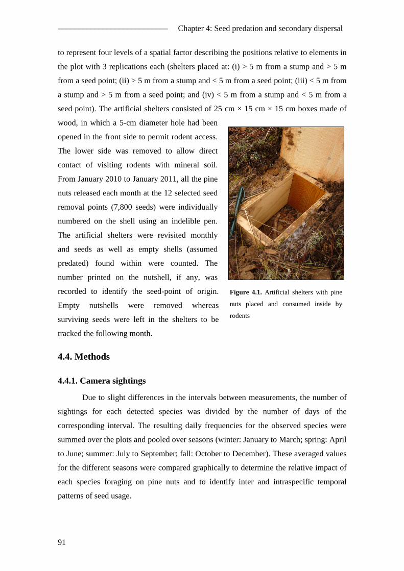
––––––––––––––––––––––––––– Chapter 4: Seed predation and secondary dispersal
91
to represent four levels of a spatial factor describing the positions relative to elements in
the plot with 3 replications each (shelters placed at: (i) > 5 m from a stump and > 5 m
from a seed point; (ii) > 5 m from a stump and < 5 m from a seed point; (iii) < 5 m from
a stump and > 5 m from a seed point; and (iv) < 5 m from a stump and < 5 m from a
seed point). The artificial shelters consisted of 25 cm × 15 cm × 15 cm boxes made of
wood, in which a 5-cm diameter hole had been
opened in the front side to permit rodent access.
The lower side was removed to allow direct
contact of visiting rodents with mineral soil.
From January 2010 to January 2011, all the pine
nuts released each month at the 12 selected seed
removal points (7,800 seeds) were individually
numbered on the shell using an indelible pen.
The artificial shelters were revisited monthly
and seeds as well as empty shells (assumed
predated) found within were counted. The
number printed on the nutshell, if any, was
recorded to identify the seed-point of origin.
Empty nutshells were removed whereas
surviving seeds were left in the shelters to be
tracked the following month.
4.4. Methods
4.4.1. Camera sightings
Due to slight differences in the intervals between measurements, the number of
sightings for each detected species was divided by the number of days of the
corresponding interval. The resulting daily frequencies for the observed species were
summed over the plots and pooled over seasons (winter: January to March; spring: April
to June; summer: July to September; fall: October to December). These averaged values
for the different seasons were compared graphically to determine the relative impact of
each species foraging on pine nuts and to identify inter and intraspecific temporal
patterns of seed usage.
Figure 4.1. Artificial shelters with pine
nuts placed and consumed inside by
rodents

––––––––––––––––––––––––––– Chapter 4: Seed predation and secondary dispersal
92
4.4.2. Seed removal
Modelling approach
As in a number of ecological processes, seed survival data from the removal
experiment are expected to show a zero-inflated distribution, meaning that on most
occasions, the majority of seed points (or at least, more than expected from the
corresponding distribution) will present zero counts (all seeds removed or destroyed).
The so-called zero-inflated models (Lambert, 1992) can deal with this kind of
distributions by simultaneously modelling the probability of event occurrence (e.g. total
removal at a seed point) and the intensity of the event conditional to occurrence, also
referred as to abundance (e.g. proportion of non-removed seeds at a seed point
providing that some seeds escaped rodent activity). In the present study we attempted to
model the process through a zero-inflated binomial model (Hall, 2000). This approach
combines two binomial distributions. The first distribution acts at seed point level and it
is used to model the probability of all seeds being removed from a seed point. The
second distribution models the probability of a single seed remaining at a seed point
(seed level) conditional to partial exploitation at seed point level. The binomial nature of
the abundance process is justified on the grounds that all seeds within a seed point hold
the same prior probability of remaining. Simultaneous estimation of parameters defining
both processes is attained through the maximisation of the likelihood function (ℓ) of the
observations, given by the product of the two abovementioned independent processes:
( ) ( ) ( )[ ]( ) ( )[ ] jkljkljkl
jkl
qynijkl
y
ijkljkl
l k j i
qnijkljkljklijkljkljkl
pp
ppy
−−−⋅⋅−×
×−⋅−+= ∏∏∏∏1
11
11,|
π
πππl
[4.1]
where πjkl is the probability of obtaining a zero count at seed point j within plot k in
month l (total exploitation at a seed point); pijkl is the probability of a seed i remaining at
a seed point j, plot k and month l; n is the initial number of seeds (50) at each seed point
j, plot k and each month l; and yjkl is the number of seeds remaining at each seed point j,
plot k and month l. qjkl is a dummy variable that equals one when a seed point j presents
a zero count in month l and zero otherwise.

––––––––––––––––––––––––––– Chapter 4: Seed predation and secondary dispersal
93
Covariate selection
Parameters π and p actually define the core processes involved in model
formulation. In order to link them to the real ecological processes underlying seed
removal, a linear model can be used to model the parameters using a set of explanatory
covariates through the logit link function. Different covariates were tested to identify
both processes based on established ecological hypothesis:
(i) Demographic stage: Cumulative precipitation over the three months prior to
each survival recording (Ppl-3) was tested, as this variable has been found to reflect the
availability of resources required to successfully overcome different stages of rodent life
(Díaz et al., 2010). We also included the physiological drought of the month in which
the measurement was taken as a covariate (Dl) to take into account the extreme summer
conditions present in the Northern Plateau. This variable was assessed as the difference
between the potential evapotranspiration and the actual maximum evapotranspiration of
month l (Thornthwaite and Mather, 1957).
(ii) Spatial location of stand elements: distance to source, seed density and
foraging preferences are factors known to possibly modify the seed shadow, and
therefore they are likely to influence the resulting distribution of seedlings. Given that
foraging choice is generally related to shelter locations, a factor considered was
proximity to stumps since these are the only protective elements in this scarce, low
diversity understory layer. In order to test these three effects, the influence potential of
all trees (IPOTtj) and stumps (IPOTsj) located within an influence area of 15 m radius
from seed points was calculated for each seed point. IPOT is a competition index based
on the concept of ecological field theory (Wu et al., 1985), empirically modified by
Kuuluvainen and Pukkala (1989):
( ) ( ) ( )tjtjtj
Nt
ttjjjj dbIIIGPOTtGPOTtIPOTt
j
⋅−×=−=−= ∏=
exp0and1where,11
( ) ( )sjsj
Ns
ssjjjj dbIIGPOTsGPOTsIPOTs
j
⋅−=−=−= ∏=
expand1where,11
Itj and Isj are the potential influence of tree t or stump s at seed point j, dtj and dsj
are the distances from tree t or stump s to seed point j, Itj(0) is dbhtj/(max dbht at each
plot), dbhtj is the diameter at breast height of tree t in the seed point j influence area, b is
a parameter assumed to equal 0.4, and Ntj and Nsj are the number of trees and stumps in
––––––––––––––––––––––––––– Chapter 4: Seed predation and secondary dispersal
94
the seed point j influence area. IPOT ranges from zero (no competition) to one
(maximum competition).
(iii) Functional response: Seed production over the two years of the study for all
four plots was predicted by means of the model proposed by Calama et al. (2011). The
beginning and length of the dispersal period were assessed using the model proposed by
Manso et al. (2012d). The weight of cones borne by trees divided by the length of the
dispersal period on a monthly basis (N0, in kg·ha-1·month-1) was used as an explanatory
variable to test the effect of varying seed production on the functional response of
rodents at stand level. The covariate entered the model as a two-order polynomial (sensu
Juliano, 2001), so that the effect is studied through an empirical approach: Type I
functional response implies that neither the linear nor the quadratic terms in the
polynomial are significant (independence of N0); Type II functional response yields a
significant and negative value for the linear term in the polynomial (the higher N0, the
lower the proportion of available seeds harvested); Type III functional response arises
when both the linear and the quadratic terms are found to be significant and are positive
and negative, respectively (comprising a certain value of N0 that maximizes seed
predation). Note that this interpretation of the sign applies directly for the occurrence
model as it predicts predation (total exploitation). In the abundance model, opposite
signs would lead to similar conclusions because this model predicts seed survival (i.e.
proportion of non-harversted seeds). The predicted seed rain was notably higher in 2010
than in 2009 in plots P2 and P7 (plot P2, 33.31 and 3.17 kg of cones·ha-1; plot P7, 34.96
and 3.33 kg of cones·ha-1). Trees in plots N1 and N2 bore slightly more cones in 2009
(14.10 and 18.05 kg of cones·ha-1) than in 2010 (13.18 and 16.87 kg of cones·ha-1).
Seeds were predicted to be released from cones from May onwards in all cases.
Overall, the evaluated expression of the two parts of the model is:
( )( ) jkjkll IPOTsβIPOTtβPpβDβNβNββ 653432
02010jkljkl 1log ++++++=− −ππ [4.2a]
( )( ) ijk653432
02010ijklijkl 1log IPOTsγIPOTtγPpγDγNγNγγpp ijkll ++++++=− − [4.2b]
where β0-6 and γ0-6 are unknown but predictable parameters related to the
aforementioned set of covariates.

––––––––––––––––––––––––––– Chapter 4: Seed predation and secondary dispersal
95
Model fitting and evaluation
Given the sampling scheme, correlation between observations that belong to the
same plot j, seed point k, and/or year m of study, as well as their interactions, might be
non-null. In order to prevent this violation of the independence assumption, random
effects for the mentioned levels of variability were included as intercept linear terms u
and v in equations [4.2a] and [4.2b], respectively. Random effects were assumed to be
normally distributed, with mean zero and variance-covariance matrix D. Due to
computing limitations, random effects were tested separately starting from the saturated
model (including all possible fixed effects) and sequentially on the models resulting
from covariate selection. The final models were evaluated in terms of Akaike
Information Criteria (AIC).
Model accuracy was evaluated by comparing predicted ( jkly ) and observed (yjkl)
values of remaining seeds at each seed point j, plot k and month l. Predictions were
obtained through the following expression ŷjkl = n × (1 – πjkl) × pjkl, where n is the initial
number of seeds at each seed point j (50 seeds), 1 – πjkl is the estimated probability of a
seed point to hold surviving seeds and pjkl is the estimated abundance at seed point
level. Mean error (E), root mean squared error (RMSE) and modelling efficiency (EF)
of the selected conditional model were calculated (equations [4.3a], [4.3b] and [4.3c]):
( )n
yyE jkl jkljkl∑ −
=ˆ
[4.3a]
( )1
ˆ2
−
−=∑
n
yyRMSE jkl jkljkl [4.3b]
( )( )∑
∑−
−−=
jkl jkljkl
jkñ jkljkl
yy
yyEF
ˆ1 [4.3c]
In addition to these indexes, a regression between observed and predicted values
( jkljkl yδδy ˆ10 += ) was computed as a measure of the level of concordance between data
and model. A successful fit of the seed removal model would imply that this regression
would be a 45º line through the origin. Therefore, the null hypothesis of δ0 = 0 and δ1 =
1 was evaluated using a simultaneous F-test (Montgomery and Peck, 1992).
––––––––––––––––––––––––––– Chapter 4: Seed predation and secondary dispersal
96
Furthermore, observed and predicted values were averaged by measurement
period at plot level and then graphically compared to test the ability of the model to
account for pure temporal variability.
All calculations were done using PROC NLMIXED in SAS 9.2.
4.4.3. Seed fate
Polar coordinates of all recovered seeds were recorded on each revisiting date of
the first fate experiment (deployment location was taken as a fixed point). The
categories described in the subsection 2.2 were used to classify seed fate. This
descriptive analysis undertaken on each visit also included the proportion of recovered
seeds and proportion of destroyed seeds. In the second seed-fate trial, distances and
final locations were controlled (artificial shelters) and therefore a generalized linear
model was fitted to the pooled data to infer the influence of shelter location and distance
to the seed source on the process. Shelter location entered the model as a factor (locikst)
of four levels accounting for the four spatial possibilities observed in the present design.
Distance of seed i within an artificial shelter to a seed point j in plot k was included as a
continuous variable (distijk). Given the nature of these data (counts), the Poisson error
structure was attempted. Alternatively, the negative binomial distribution was also
considered in order to deal with overdispersion problems. For both distributions, the log
link function was used. The expanded expression of this model is:
( ) ijkikstijkst distλlocλd 10log ++= [4.4]
where dijkst is the sum of all seeds i placed within a given artificial shelter in plot k with
a closest seed point j, stump s and tree t. λ0-1 are parameters to be estimated. A
sequential variable selection was carried out. The performance of the two models fitted
with the Poisson and negative binomial distribution respectively was tested through the
comparison of their resulting AICs. This analysis was performed using R 2.14 (R Core
Team, 2011).
4.5. Results
4.5.1. Camera sightings
Overall, 1,335 videos of fauna feeding on P. pinea seeds were recorded. The
vast majority (80%) corresponded to the wood mouse (A. sylvaticus) whereas the azure-

––––––––––––––––––––––––––– Chapter 4: Seed predation and secondary dispersal
97
winged magpie (Cyanopica cyanus Pallas) was observed in 16% of sightings. Much less
frequent was the carrion crow (Corvus corone L.; 4%) and the common crossbill (Loxia
curvirostra L.; <1%). Frequencies changed seasonally, with a minimum for A.
sylvaticus in summer, the opposite being
the case for C. cyanus (Fig. 4.2). C.
corone mostly appeared in spring.
From a behavioural perspective,
A. sylvaticus normally took only few
seconds to select a single targeted seed,
which was either consumed in situ or
removed from the field of vision of the
cameras. Contrastingly, birds always
took seeds to a different location and
took longer to make their selection than
the wood mice. The number of pine nuts
per flight was commonly two in the case
of C. cyanus, whereas C. corone
collected up to five seeds.
4.5.2. General pattern of seed removal
From a temporal perspective, with few exceptions, most seed points were
completely exploited from October/November to May/June in both years of study (Fig.
4.3). Specifically, in 49 surveys (out of 112 = four plots × 28 visits/plot) there were no
seeds to be found at the original placement. Additionally, it was found that during
certain periods, normally the warmer months (which tend to be a “safe” period for
seeds), seed removal either ceased completely or was much reduced (less than 10% of
seeds removed). As regards locations, plots P2 and P7 shared a similar pattern, with a
longer safe period in 2010 (May to February (2011) and June to January (2011)) than in
2009 (June to September and July to September), the latter exhibiting a lower mean
proportion of remaining seeds (mean and standard error for 2009 and 2010,
respectively: plot P2, 0.31±0.03, 0.61±0.03; plot P7, 0.42±0.04, 0.81±0.02).
Contrastingly, plot N2 showed the opposite trend with a longer safe period and higher
levels of intact seeds in 2009 than in 2010 (May to November (0.78±0.03) and July to
August (0.46±0.06), respectively). The process in plot N1 emulated the pattern of plots
Figure 4.2. Frequencies of daily animal
sightings pooled over seasons. Dark, medium
and light grey bars represent Apodemus
sylvaticus, Cyanopica cyanus and Corvus
corone values, respectively
––––––––––––––––––––––––––– Chapter 4: Seed predation and secondary dispersal
98
P2 and P7 in 2009 (May to September (0.35±0.03)) and was closer to that of plot N2 in
2010 (June to October (0.44±0.06)).
As shown in Fig. 4.3, the occurrence of physiological drought loosely coincided
with those periods of less removal activity and, in general, seed exploitation increased
along with three-month cumulative precipitation.
4.5.3. Seed removal model
The variance structure accounting for seed point × year random variability
proved the most appropriate for the current data set in terms of AIC (Table 4.2). In the
sequential fixed effects selection carried out under this structure, different covariates
resulted non-significant and therefore were dropped from the model. Regarding the
occurrence part of the model, the parameter linked to IPOTs was not found to
statistically differ from zero. Consequently, the probability of absolute predation
occurrence in a seed point j and plot k for a given month l (πjkl) is explained by seed
production (N0), physiological drought (Dl) and cumulative precipitation three months
Figure. 4.3. Mean number of remaining seeds (solid line), physiological drought (D, in mm, dotted
line) and cumulative precipitation of the three previous months (Ppl-3, in cm, dashed line) over time for
plots P2 (a), P7 (b), N1 (c) and N2 (d)
––––––––––––––––––––––––––– Chapter 4: Seed predation and secondary dispersal
99
prior to predation event (Ppl-3) at temporal level, and proximity to trees (IPOTt) at
spatial level. The sign of the parameters indicates that the higher the physiological
drought and seed production and the lower the precipitation (Table 4.3), the lower the
likelihood that total exploitation will occur. A positive IPOTt parameter implies higher
removal in the proximity of trees.
Table 4.2. Fit statistics for the different random structure alternatives tested. In bold, values
corresponding to the preferred model
random level seed point plot year* year × seed point year × plot
–2LL a 38,509 38,728 - 36,641 37,378
AICb 38,531 38,750 - 36,665 37,402
a–2LL: minus twice the logarithm of the maximum likelihood estimate; bAICb: Akaike Information Criterium; *: lack of stable convergence
Table 4.3. Summary of parameter estimates and significance for the selected model, including variance
components of the random effects
occurrence of zero counts (β) abundance of survival (γ)
covariate estimate p-value estimate p-value
Intercept 1.9769 < 0.0001 – 0.9589 < 0.0001
N0a – 0.6301 < 0.0001 0.2946 < 0.0001
Dlb – 0.0547 < 0.0001 0.0164 < 0.0001
Ppl-3c 1.8830 0.0024 - -
IPOTtjd 0.0087 0.0003 - -
IPOTsje - - – 0.6410 < 0.0001
σ2uf 1.5904 - - -
σ2vg - - 1.1562 -
σuvh – 0.6858 - – 0.6858 -
aN0: variable linked to seed dispersal;bDl: physiological drought; cPpl-3: cumulative precipitation of the three previous months; dIPOTt and eIPOTs: tree and stump IPOT indexes; fσ2
u and gσ2v: estimated variances associated to
the random intercepts (see point × year level); hσuv: covariance between both random effects.
As regards the abundance of remaining seeds (pijkl), Ppl-3 and IPOTtj were non-
significant. However, in consistence with the effects observed in the occurrence
subprocess, increasing drought intensity and large crop size limit seed removal.
Furthermore, seeds are harvested more rapidly in the proximity of stumps, as the
parameter related to IPOTsj adopted a negative value. Finally, in both occurrence and
abundance submodels, the quadratic term in the polynomial function of seed production
was non-significant, inferring a Type II functional response at stand level. The final
parameterization is shown in Table 4.3. Note that opposite signs in parameters linked to
the same covariates in equations [2a] and [2b] reveals a common tendency, as πjkl
represents the probability of total exploitation whereas pijkl stands for the probability of
––––––––––––––––––––––––––– Chapter 4: Seed predation and secondary dispersal
100
seed survival conditional to 1 – πjkl. This is also consistent with the negative value
obtained for the covariance between random effects affecting the respective intercepts
of equations [2a] and [2b].
The model proved highly accurate, with EF = 68.61%, E = 0.1171 surviving
seeds·(seed point·month)-1 and RMSE = 10.2286 seeds·(seed point·month)-1. As regards
the regression between observed and predicted values, the null hypothesis of intercept
and slope parameters not differing from zero and one respectively was not rejected (F =
1.0093; p-value = 0.3647), confirming that the model was unbiased. At temporal level,
Fig. 4.4 shows how the model closely mimics the pattern of seed removal, perfectly
capturing the existing seasonal variability in each plot.
Figure. 4.4. Observed (dashed line) and predicted values (solid line) of mean number of remaining
seeds per seed point over time in sampling plots P2 (a), P7 (b), N1 (c) and N2 (d)
––––––––––––––––––––––––––– Chapter 4: Seed predation and secondary dispersal
101
4.5.4. Seed fate
As regards the first experiment, all seeds recovered following release on 11
December 2009 had been completely exploited by rodents when the plots were revisited
on 19 January 2010. The fate of seeds from the second attempt (set up on 19 January
2010) was checked on 28 January, 8 February and 16 March 2010. In this case, the
small number of seeds that escaped rodent predation during the first week of exposition
was found to be either unaltered at the original position, larder-hoarded or scattered on
the ground at short distances from the deployment point (mean distance 3.16 m).
Surviving seeds were mostly exploited by rodents in subsequent visits. These results are
detailed in Fig. 4.5.
In the second experiment, 1227 seeds (out of which 79% were marked) were
recovered from the artificial shelters. 89% of cached seeds were consumed within the
boxes immediately after relocation and those that survived were found to have been
predated within the next month. One exception to this pattern was a shelter containing
38 seeds, which was undisturbed for two consecutive months. The seeds in this shelter
germinated and consequently escaped predation. The number of cached seeds over time
shared a common pattern from one plot to another, with higher values in autumn and
spring. Seed caching was maximum in plot P2 in March 2010 (3.86 seeds·day-1) and in
December 2010 (1.27 seeds·day-1). Maximum values in plot N1 were reached in
December 2009 (5.2 seeds·day-1), May 2010 (5.6 seeds·day-1) and November 2011 (5.3
seeds·day-1). The monthly ratio between non-predated and predated seeds was only
higher than one in summer. As regards the fitted model, the Poisson distribution could
not account for the overdispersion present in our data and therefore the negative
binomial distribution proved significantly more adequate (Table 4.4). In the final model,
only distance from the shelter to the closest seed point was significant. The associated
parameter was negative, meaning that there is less likelihood of finding dispersed seeds
as distance from the place of collection increases (Table 4.4).

––––––––––––––––––––––––––– Chapter 4: Seed predation and secondary dispersal
102
Table 4.4. Selection process for the seed fate model. p-values of the different variables and parameter
values for the preferred model are given (in bold)
Poisson model negative binomial model parameter value variable/statistic 1 2 1 2
Intercept < 0.0001 < 0.0001 < 0.0001 < 0.0001 4.6049
locikst,2a 0.0007 - 0.5200 - -
locikst,3 0.2181 - 0.8060 - -
locikst,4 0.0371 - 0.9650 - -
distijkb < 0.0001 < 0.0001 0.2730 0.00859 – 0.1517
θc 1* 1* 1.248 1.222 1.222
– 2LLd 868.73 888.07 229.90 230.46 -
AICe 878.73 898.07 241.9 236.46 - alocikst: 4-level factor accounting for seed location in regard to trees and stumps; bdistijk: distance from seed location to the nearest seed station; cθ: parameter modelling overdispersion: when set fixed to 1 (*) a Poisson distribution is
used; otherwise, a negative binomial distribution is utilized. d– 2LL is minus twice the logarithm of the maximum likelihood estimate and eAIC is the Akaike Information Criterium
4.6. Discussion
4.6.1. The role of A. sylvaticus in P. pinea natural regeneration
In the present study, we attempted to describe and predict the spatio-temporal
interactions between A. sylvaticus and P. pinea. This general purpose gives rise to the
first question addressed in this paper: what role does this rodent species play in the
natural regeneration of P. pinea forests throughout the Northern Plateau of Spain?
Although we found evidence suggesting a marginal (and potentially effective) dispersal
activity, our seed fate experiments provided overwhelming evidence that confirmed our
hypothesis of a predominant predator-prey interaction. This fact appears to be a
common trend in other Mediterranean large-seeded tree species. In this respect, our
results are consistent with those reported by Gómez et al. (2003) for ecological
interactions between Apodemus spp. and Quercus pyrenaica. Identically, Gómez et al.
(2008) determined that A. sylvaticus consumed over 98% of the Quercus ilex seeds
deployed and also pointed to the potential benefits associated with the dispersal of a
small (albeit minimal) fraction of the seeds. Hulme (1997) observed the same behavior
in this species when foraging on different food sources in south-eastern Spain. In the
following paragraphs we shall further discuss the association of A. sylvaticus with P.
pinea and attempt to analyze the plant developed strategies underlying the coexistence
of both species.

––––––––––––––––––––––––––– Chapter 4: Seed predation and secondary dispersal
103
4.6.2. Seed removal
Seed predation temporal pattern
Our results reveal that seed predation is indirectly controlled by climate on a
temporal scale through two mechanisms. On the one hand, water availability appears to
account for within-year seed predation rates, leading to a safe period during the months
of water shortage. The reason for this is the strong dependence of A. sylvaticus
populations on short-term prior precipitation conditions, which in turn are a surrogate of
primary productivity, as reported by Díaz et al. (2010) for north-western Spain. This
dependence on climatic conditions is also revealed by the significant influence of
drought intensity as an additional factor explaining food limitation, probably resulting
from the more extreme conditions of central Spain. Rodent population reduction in the
study area during the summer period is confirmed by the consequent decrease in the
number of A. sylvaticus individuals in our recorded videos. On the other hand, A.
sylvaticus proved highly sensitive to the occurrence of masting events, a between-year
climate-mediated process in P. pinea (Mutke et al., 2005a; Calama et al., 2011). Dual
climate prey-predator control of this type has been identified in alpine ecosystems,
enhancing fitness in European larch (Poncet et al., 2009), which suggests that the
described pattern may be common, at least in limiting environments. Nevertheless, it
should be noted that a non-negligible fraction of the observed between-year and spatial
variability in seed predation is attributable to the stochasticity of the process, as
indicated by the non-null random variance at seed point × year level.
The resulting parameterization of seed production as a covariate explaining
predation also shed light on the shape of the functional response of A. sylvaticus at stand
scale. On the one hand, the predicted Holling Type II response indicates that there is a
greater chance of seeds escaping predation with increasing seed production (for
instance, when mast seed crops are produced). This supports the predator satiation
hypothesis (Salisbury, 1942; Janzen, 1974), which is expected in low diversity plant
communities where among-individual synchrony in fecundity occurs (Nilsson and
Wastljung, 1987; Homma et al., 1999) and where the frugivore present is not primarily
a mutualist (Hulme and Hunt, 1999; Vander Wall, 2002), as is clearly the case in our
study. On the other hand, Type II response would also suggest that the studied predator
is a specialist (Andersson and Erlinge, 1977), in contrast with the behaviour commonly

––––––––––––––––––––––––––– Chapter 4: Seed predation and secondary dispersal
104
exhibited by A. sylvaticus (Díaz et al., 2010). The most likely explanation in this case is
that A. sylvaticus is acting as a specialist with respect to this particular source of food.
In this regard, generalists are able to switch from one food source to another when the
preferred source is scarce. However, when the preferred food is notably more
palatable/nutritive than others, it is possible that frequency dependence does not occur
at low crop densities (Hulme and Hunt, 1999) and therefore the generalist continues
foraging preferentially on the same crop, leading to total exploitation of exposed seeds
and even to instability of the system (Murdoch, 1969; Murdoch and Oaten, 1975). This
may be the case of A. sylvaticus and the highly nutritive P. pinea seeds in periods of
pine nut scarcity.
Seed predation spatial pattern
From a spatial perspective, A. sylvaticus was distance dependent with respect to
seed sources. As a consequence of the higher predation rates in the close vicinity of
trees, recruitment might be expected to occur at relatively large distances from seed
sources (Janzen-Connell hypothesis; Janzen, 1970; Connell, 1971). However, Calama et
al. (2012) identified a clumped distribution of one-year-old P. pinea seedlings beneath
the tree crowns, suggesting that the spatial distribution of predator activity does not
qualitatively alter the P. pinea seed shadow. This fact is ecologically consistent with the
findings of these authors, who stated that seedling survival was also higher under the
canopy. Therefore, those locations which offer the highest probability of offspring
survival are also those with the greatest probability of seed occupation after predation.
Seeds were also more rapidly predated in the proximity of the potential natural
shelters identified (stumps). This finding is consistent with those reported in other
studies concerned with spatial foraging preferences in A. sylvaticus, reflecting the
preference of this species for protected feeding areas (Hulme, 1997; Fedriani and
Manzaneda, 2005).
4.6.3. Secondary seed dispersal
It has been reported that masting promotes animal-mediated seed dispersal
because hoarding animals are able to cache excessive amounts of food in order to
withstand unfavourable periods (Vander Wall, 2002). No evidence of such behaviour
was detected in our experiments, which supports the results of other studies conducted
in the Iberian Peninsula (Hulme, 1997; Gómez et al., 2003; Gómez et al., 2008) even

––––––––––––––––––––––––––– Chapter 4: Seed predation and secondary dispersal
105
though in its southernmost distribution area, A. sylvaticus usually coexists with masting
species. The fact that A. sylvaticus acts mainly as a predator would suggest that cached
resources are not further required, as the seed dispersal period in P. pinea (warm period)
is immediately followed by the favourable period for the rodent species (colder period)
(Torre et al., 2002; Díaz et al., 2010).
Despite the limited extent of animal-mediated dispersal according to our data, a
number of conclusions can be drawn with regard to the effectiveness of the small
fraction of surviving, animal dispersed seeds. Scatter-hoarding of P. pinea seeds seems
to be a rarely used mechanism in A. sylvaticus, as previously suggested by Hulme
(2002) with regard to rodents (excepting squirrels). Furthermore, when scatter-hoarding
occurs, our observations revealed rapid pilfering and immediate consumption of the
cached seed. Larder-hoarding was much more frequent although probably ineffective as
a dispersal mechanism. Such hoards were normally used as very short-term reserves.
Moreover, those seeds that remain in caches at very high densities (until the arrival of
the unfavourable period for rodents, escaping predation through early germination) are
not expected to produce viable seedlings due to interspecific competition (Hulme, 2002;
Gómez et al., 2003). Furthermore, the model fitted using the artificial-shelter data
indicates that A. sylvaticus only larder-hoards up to very short distances, displaying no
particular habitat preference, which suggests that the impact on final seedling shadow
would be of little importance.
As regards other guilds of possible dispersers, there were far fewer camera
sightings of C. cyanus and C. coronae than of A. sylvaticus and therefore the impact of
potential dispersal on managed forest dynamics would be limited. However, corvids are
well-known dispersers (Vander Wall, 2002; Gómez, 2003) and most visits coincided
with the dispersal period of P. pinea, suggesting possible hoarding behaviour of birds,
presumably attracted by seed abundance as described in Vander Wall (2002). The
behaviour exhibited by the birds in the recorded videos, in which seeds were never
predated in situ but removed somewhere else. Although beyond the scope of this
particular study, the importance of these birds should not be overlooked from an
ecological viewpoint.
––––––––––––––––––––––––––– Chapter 4: Seed predation and secondary dispersal
106
4.6.4. The Apodemus sylvaticus-Pinus pinea interaction
The results of this study highlight the strong influence of climate in regulating
the coexistence of A. sylvaticus and P. pinea through two complementary strategies: on
the plant side, seeds are able to escape predation for a period of several months (i)
concentrating dispersal in the unfavourable period for rodent populations; and (ii)
producing mast pulses that notably increase the fraction of non-predated seeds during
the aforementioned period. Therefore, it may be inferred that the dispersal strategy
developed by P. pinea is an adaptation mediated by the specialist-like behaviour of A.
sylvaticus when feeding on P. pinea seeds. This selective pressure of A. sylvaticus
would be more important at within-year level, given the climatic origin of P. pinea
masting habit.
The abovementioned strategy alone, however, does not guarantee the persistence
of P. pinea: on the animal side, fluctuations in A. sylvaticus populations mainly depend
on primary productivity, the numerical recovery of which at the end of the dry period
results in rapid depletion of previously dispersed seeds. Given the strict conditions
required for seed germination in the species (Manso et al., 2012c; in press), conditions
which normally coincide with early fall (Calama et al., 2012), the window for
emergence and subsequent establishment is especially narrow. Due to the high
stochasticity generally associated with ecological processes, it can be concluded that the
predatory pressure exerted by A. sylvaticus could dramatically condition P. pinea
natural regeneration at annual level.
However, the intense and non-progressive fellings carried out in the managed P.
pinea forests of the Northern Plateau of Spain, severely reduce the likelihood of
adequate conditions for establishment in the long term. This situation may underlie the
observed natural regeneration failure in managed forests. As regards a future climatic
scenario of increasing drought intensity and length in central Spain (De Castro et al.,
2005), predation levels might be expected to decrease although seed production and
germination may also be seriously constrained (Manso et al., 2012c; in press).
Therefore, further research needs to be conducted in this field in order to shed more
light on this particular matter.

–––––––––––––––––––––––––––––––––––––––––––––––––––––––––––––– Chapter 4: Post-dispersal seed predation and secondary dispersal
107
Figure 4.5. Results of the seed fate experiment. Each box represents a specific state for a particular number of seeds and specific date (left). In brackets, the corresponding
proportion over the total. Possible states: TS: Total Seeds; P: Predated; NP: No Predated; L: Lost; P-IS: Predated In Situ; P-M: reMoved and Predated; P-SH: Scatter-Hoarded
and Predated; P-LH: Larder-Hoarded and Predated; IS: In Situ; M: reMoved; LH: Larder-Hoarded. In bold, terminal states
–––––––––––––––– Chapter 4: Post-dispersal seed predation and secondary dispersal
108
References
Andersen, A. N. (1987) Effects of seed predation by ants on seedling densities at a woodland site in SE Australia. Oikos, 48, 171-174.
Andersson, M. & Erlinge, S. (1977) Influence of predation on rodent populations. Oikos, 29, 591-597.
Calama, R., Madrigal, G., Manso, R., Garriga, E., Gordo, F. J. & Pardos, M. (2012) Germinación, emergencia y supervivencia de regenerado en Pinus pinea L. La regeneración natural de los pinares en los arenales de la Meseta Castellana (eds J. Gordo, R. Calama, M. Pardos, F. Bravo & G. Montero). Instituto Universitario de Investigación en Gestión Forestal Sostenible (Universidad de Valladolid-INIA), Valladolid.
Calama, R., Mutke, S., Tomé, J., Gordo, J., Montero, G. & Tomé, M. (2011) Modelling spatial and temporal variability in a zero-inflated variable: The case of stone pine (Pinus pinea L.) cone production. Ecological Modelling, 222, 606-618.
Castro, J., Gómez, J. M., García, D., Zamora, R. & Hodar, J. A. (1999) Seed predation and dispersal in relict Scots pine forests in southern Spain. Plant Ecology, 145, 115-123.
Connell, J. H. (1971) On the role of natural enemies in preventing competitive exclusion in some marine animals and in rain forest trees. Dynamics of Numbers in Populations (Proceedings of the Advanced Study Institute, Osterbeek 1970) (eds P. J. Boer & G. R. Graadwell), pp. 298-312. Centre for Agricultural Publication and Documentation, Wageningen
Crawley, M. J. & Long, C. R. (1995) Alternate bearing, predator satiation and seedling recruitment in Quercus robur L. Journal of Ecology, 83, 683-696.
Curran, L. M. & Leighton, M. (2000) Vertebrate responses to spatiotemporal variation in seed production of mast-fruiting dipterocarpaceae. Ecological Monographs, 70, 101-128.
De Castro, M., Martín-Vide, J. & Alonso, S. (2005) The climate of Spain: past, present and scenarios for the 21st century. A preliminary assessment of the impacts in Spain due to the effects of climate change. ECCE Project-Final report, pp. 1-64. Ministerio de Medio Ambiente, Madrid.
De Steven, D. (1982) Seed production and seed mortality in a temperate forest shrub (witch-hazel, Hamamelis virginiana). Journal of Ecology 70, 437-443.
Díaz, M., Torre, I. & Arrizabalaga, A. (2010) Relative roles of density and rainfall on the short-term regulation of Mediterranean wood mouse Apodemus sylvaticus populations. Acta Theriologica, 55, 251-260.
Fedriani, J. M. & Manzaneda, A. J. (2005) Pre- and postdispersal seed predation by rodents: balance of food and safety. Behavioral Ecology, 16, 1018-1024.
Gómez, J. M. (2003) Spatial patterns in long-distance dispersal of Quercus ilex acorns by jays in a heterogeneous landscape. Ecography, 26, 573-584.
Gómez, J. M., García, D. & Zamora, R. (2003) Impact of vertebrate acorn- and seedling-predators on a Mediterranean Quercus pyrenaica forest. Forest Ecology and Management, 180, 125-134.
Gómez, J. M., Puerta-Piñero, C. & Schupp, E. W. (2008) Effectiveness of rodents as local seed dispersers of Holm oaks. Oecologia, 155, 529-537.
González-Rodríguez, V. & Villar, R. (2012) Post-dispersal seed removal in four Mediterranean oaks: species and microhabitat selection differ depending on large herbivore activity. Ecological Research, 27, 587-594.
–––––––––––––––– Chapter 4: Post-dispersal seed predation and secondary dispersal
109
Hall, D. B. (2000) Zero-inflated Poisson and binomial regression with random effects: A case study. Biometrics, 56, 1030-1039.
Hernández, L., Rubiales, J. M., Morales-Molino, C., Romero, F., Sanz, C. & Gómez Manzaneque, F. (2011) Reconstructing forest history from archaeological data: A case study in the Duero basin assessing the origin of controversial forests and the loss of tree populations of great biogeographical interest. Forest Ecology and Management, 261, 1178-1187.
Herrera, C. M. (1995a) Plant-vertebrate seed dispersal systems in the Mediterranean: ecological, evolutionary and historical determinants. Annual Review of Ecology and Systematics, 26, 705-727.
Herrera, C. M., Jordano, P., Guitian, J. & Traveset, A. (1998) Annual variability in seed production by woody plants and the masting concept: Reassessment of principles and relationship to pollination and seed dispersal. American Naturalist, 152, 576-594.
Herrera, J. (1995b) Acorn predation and seedling production in a low-density population of cork oak (Quercus suber L.). Forest Ecology and Management, 76, 197-201.
Holling, C. S. (1959a) The components of predation as revealed by a study of small-mammal predation of the European pine sawfly. The Canadian Entomologist, 91, 293-320.
Holling, C. S. (1959b) Some characteristics of simple types of predation and parasitism. The Canadian Entomologist, 91, 385-398.
Homma, K., Akashi, N., Abe, T., Hasegawa, M., Harada, K., Hirabuki, Y., Irie, K., Kaji, M., Miguchi, H., Mizoguchi, N., Mizunaga, H., Nakashizuka, T., Natume, S., Niiyama, K., Ohkubo, T., Sawada, S., Sugita, H., Takatsuki, S. & Yamanaka, N. (1999) Geographical variation in the early regeneration process of Siebold's Beech (Fagus crenata BLUME) in Japan. Plant Ecology, 140, 129-138.
Hulme, P. E. (1997) Post-dispersal seed predation and the establishment of vertebrate dispersed plants in Mediterranean scrublands. Oecologia 111, 91-98.
Hulme, P. E. (2002) Seed-eaters: seed dispersal, destruction and demography. Seed dispersal and frugivory: Ecology, Evolution and Conservation (eds D. J. Levey, W. R. Silva & M. Galetti), pp. 257-273. CAB International, Wallingford.
Hulme, P. E. & Hunt, M. K. (1999) Rodent post-dispersal seed predation in deciduous woodland: predator response to absolute and relative abundance of prey. Journal of Animal Ecology, 68, 417-428.
Janzen, D. H. (1970) Herbivores and the number of tree species in tropical forests. American Naturalist 104, 501-528.
Janzen, D. H. (1974) Tropical blackwater rivers, animal and mast fruiting by the Dipterocarpaceae. Biotropica, 4, 69-103.
Jordano, P. (1992) Fruits and frugivory. Seeds: the ecology of regeneration in natural plant communities (ed M. Fenner), pp. 105-156. CAB International, Wallingford.
Juliano, S. A. (2001) Non-linear curve-fitting: predation and functional response curves. Design and Analysis of Ecological Experiments (eds S. M. Scheiner & J. Gurevitch), pp. 178-196. Chapman & Hall, New York.
Kelly, D. & Sork, V. L. (2002) Mast seeding in perennial plants: Why, how, where? Annual Review of Ecology and Systematics, 33, 427-447.
Klinger, R. & Rejmanek, M. (2009) The numerical and functional responses of a granivorous rodent and the fate of Neotropical tree seeds. Ecology, 90, 1549-1563.

–––––––––––––––– Chapter 4: Post-dispersal seed predation and secondary dispersal
110
Kratina, P., Vos, M., Bateman, A. & Anholt, B. R. (2009) Functional responses modified by predator density. Oecologia, 159, 425-433.
Kuuluvainen, T. & Pukkala, T. (1989) Effect of Scots pine seed trees on the density of ground vegetation and tree seedlings. Silva Fennica, 23, 159-167.
Lambert, D. (1992) Zero-inflated Poisson regression, with an application to defects in manufacturing. Technometrics, 34, 1-14.
Manso, R., Fortin, M., Calama, R. & Pardos, M. (2012c) Modelling seed germination in forest tree species through survival analysis. The Pinus pinea L. case study. Forest Ecology and Management, in press.
Manso, R., Pardos, M., Keyes, C. R. & Calama, R. (2012d) Modelling the spatio-temporal pattern of primary dispersal in stone pine (Pinus pinea L.) stands in the Northern Plateau (Spain). Ecological Modelling, 226, 11-21.
Montgomery, D. C. & Peck, E. A. (1992) Introduction to Linear Regression Analysis. Wiley, New York.
Morales, L. (2009) Modelos para la predicción del contenido y calidad de piñón en piñas de Pinus pinea L. en los valles del Tiétar y del Alberche. Master Thesis, Universidad Politécnica de Madrid, Madrid.
Murdoch, W. W. (1969) Switching in general predators. Experiments on predator specificity and stability of prey populations. Ecological Monographs, 39, 335-&.
Murdoch, W. W. & Oaten, A. (1975) Predation and population stability. Advances in Ecological Research, 9, 1-131.
Mutke, S., Gordo, J. & Gil, L. (2005a) Variability of Mediterranean Stone pine cone production: Yield loss as response to climate change. Agricultural and Forest Meteorology, 132, 263-272.
Nathan, R. & Casagrandi, R. (2004) A simple mechanistic model of seed dispersal, predation and plant establishment: Janzen-Connell and beyond. Journal of Ecology, 92, 733-746.
Nilsson, S. G. & Wastljung, U. (1987) Seed predation and cross-pollination in mast-seeding beech (Fagus sylvatica) patches. Ecology, 68, 260-265.
Poncet, B. N., Garat, P., Manel, S., Bru, N., Sachet, J.-M., Roques, A. & Despres, L. (2009) The effect of climate on masting in the European larch and on its specific seed predators. Oecologia, 159, 527-537.
Puerta-Piñero, C., Gómez, J. M. & Schupp, E. W. (2010) Spatial patterns of acorn dispersal by rodents: do acorn crop size and ungulate presence matter? Oikos, 119, 179-187.
R Core Team (2011) R: A language and environment for statistical computing. R Foundation for Statistical Computing, Vienna, Austria.
Salisbury, E. J. (1942) The reproductive capacity of plants. Bell, London. Schupp, E. W. (1995) Seed-seedling conflicts, habitat choice, and patterns of plant
recruitment. American Journal of Botany, 82, 399-409. Schupp, E. W. & Fuentes, M. (1995) Spatial patterns of seed dispersal and the
unification of plant population ecology. Ecoscience, 2, 267-275. Sork, V. L. (1993) Evolutionary ecology of mast-seeding in temperate and tropical oaks
(Quercus spp.). Vegetatio, 108, 133-147. Thornthwaite, C. W. & Mather, J. R. (1957) Instructions and tables for computing
potential evapotranspiration and the water balances. Climatology 10, 181-311. Torre, I., Arrizabalaga, A. & Díaz, M. (2002) Ratón de campo (Apodememus sylvaticus
L.). Galemys, 14.

–––––––––––––––– Chapter 4: Post-dispersal seed predation and secondary dispersal
111
van Leeuwen, E., Jansen, V. A. A. & Bright, P. W. (2007) How population dynamics shape the functional response in a one-predator-two-prey system. Ecology, 88, 1571-1581.
Vander Wall, S. B. (2002) Masting in animal-dispersed pines facilitates seed dispersal. Ecology, 83, 3508-3516.
Wu, H. I., Sharpe, P. J. H., Walker, J. & Penridge, L. K. (1985) Ecological field-theory-A spatial-analysis of resource interference among plants. Ecological Modelling, 29, 215-243.

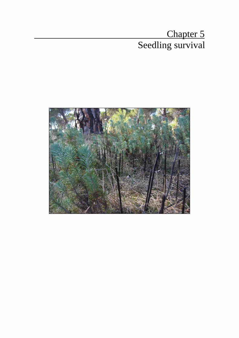
Chapter 5 Seedling survival


5. Seedling survival Based on:
Manso, R., Calama, R., Madrigal, G., Conde, M., Gordo, F. J. & Pardos, M. (2012) Supervivencia del regenerado en Pinus pinea L. en la Meseta Norte. Previsiones en un contexto de cambio climático. V Reunión del Grupo de Trabajo de Selvicultura de la Sociedad Española de las Ciencias Forestales (SECF) "Regeneración natural y cambio global" (eds R. Ruiz-Peinado, J. Reque & R. Serrada). Sociedad Española de Ciencias Forestales, Madrid. in press.
Specific objectives:
1. Selecting variables to include in the different submodels that are easily-accessible or
controllable by forest managers so that the final model can truly constitute a decision-
making tool
5.- Modelling the temporal transition probability of seedlings to survive
6. Identifying the potential bottlenecks that could affect natural regeneration at
subprocess level, taking into consideration the silvicultural practices and the ecological
processes involved
Data:
- Seedling occurrence and survival data series (2004-2011) from plots P1 to P6 from the
natural regeneration INIA site in La Pedraja de Portillo (Valladolid)
Methodology:
- Proportional-hazards model
Main findings:
- When cohorts are generated in fall, seedling mortality was extremely high during the
first months, the number of surviving seedlings being stabilised after two years
- Contrastingly, almost no seedling appeared in spring survived the summer season,
suggesting that drought is a limiting factor for seedling survival
Management implications:
- Given that only abundant cohorts occurred in fall are expected to produce a relevant
number of persistent seedlings, seedling survival could become a bottleneck for natural
regeneration
- Present strict and intensive regeneration fellings are currently conducted without
considering these findings and, therefore, flexibility is needed in this respect until
cohorts can be considered as established


––––––––––––––––––––––––––––––––––––––––––––– Chapter 5: Seedling survival
117
5. Seedling survival
5.1. Abstract
The current study intends to model seedling survival of Pinus pinea L. in the
Northern Plateau of Spain, as well as to identify the key factors that determine seedling
mortality. These findings will make it possible to infer recommendations for silviculture
under both the present and future climate. For the purposes of this research, survival of
different cohorts has been surveyed from 2004 to date in P. pinea even-aged stands
located in the sandy flats of the province of Valladolid. Data were analyzed through a
proportional-hazards model, based on the cohorts occurred in fall. The effect of drought
on these cohorts was also considered. The use of the latter as an explanatory variable
leads to unrealistic predictions, which suggests that most of the variability is accounted
for seedling age. Survival of autumn seedlings during the first year is lower than 20%,
the surviving individuals being stabilized in 4% of the emerged seedlings from the
second year onwards. In the case of seedlings appearing in spring, almost none of them
overcame the first summer, suggesting that drought is behind mortality in these cohorts.
In a scenario of climatic change, it would be likely that drought impact would also
affect the seedlings from the previous fall period. Given the predicted high mortality
rates, current silviculture schedules should become more flexible, allowing the
occurrence of an enough number of cohorts to guarantee successful recruitment.
Keywords: survival analysis, seedling mortality, drought, stone pine

––––––––––––––––––––––––––––––––––––––––––––– Chapter 5: Seedling survival
118
5.2. Introduction
Seedling mortality represents a major cause for natural regeneration failure in
Mediterranean forests (Calama and Montero, 2007). In the case of Pinus pinea L.,
where bottlenecks for regeneration are expected in all the processes involved (seed
production (Calama et al., 2011); seed dispersal (Manso et al., 2012d); germination
(Manso et al., 2012c; in press); and seed predation (Manso et al., 2012b), seedling
survival has become a major concern for forest managers. Specifically, it is of crucial
importance the impact of summer drought on seedling survival, as water availability is
acknowledged as the most serious constraining factor in the Mediterranean (Blondel and
Aronson, 1999).
As a consequence, there is an urgent necessity of modelling the process through
realistic and accessible models as a management tool. Regression models based on
survival analysis techniques have been successfully used for that purpose in studies on
seedling survival (Selander, 1993).
The main aims of the present paper are (i) modelling the seedling survival
process; (ii) identifying the variables involved; and (iii) providing silviculture
alternatives that guarantee natural regeneration. We hypothesized that (i) summer
drought drastically conditions recruitment; and that (ii) seedling mortality could be
partially behind the natural regeneration failure of the species in the Northern Plateau of
Spain.
5.3. Material and methods
5.3.1. Study site
The study site is located in the Tierra de Pinares county, province of Valladolid,
in the municipality of La Pedraja de Portillo (41º28’N, 4º43’W), at an altitude of 700 m
above sea level. The study was conducted in a P. pinea pure even-aged stand (Corbejón
y Quemados public forest), representative of the regional average conditions
(Mediterranean-continental climate and sandy soils). Specifically the experiment was
set up in a 120-years-old regeneration block and site index 15–16 m at 100 years,
characteristic of a II class quality (Calama et al., 2003). Seeding felling were carried out
in 2002–2003.

––––––––––––––––––––––––––––––––––––––––––––– Chapter 5: Seedling survival
119
5.3.2. Experimental design
The experiment, set up in 2003, consists of six 60 m × 80 m plots (0.48 ha each),
with a 7.5 m buffer area outwards, where two regeneration systems were applied (the
shelterwood system (SW; plots P4-P6) and the seed-tree system (ST; plots P1-P3)),
implying three replications each. Additionally, a control plot was also established. Stand
density and basal area (BA) in the control (P7) is 149 stems·ha-1 (18.42 m2·ha-1).
Otherwise, stand density ranges from 73–75 stems·ha-1 (BA 9.70–12.26 m2·ha-1), in the
plots where the SW system was applied, to 46–48 stems·ha-1 (BA 6.99–9.37 m2·ha-1) in
those plots were the ST system was used. Trees in all plots were mapped and their dbh
(1.30 m) measured.
Twenty 3 m × 3 m subplots were established on a regular grid across all plots
(140 subplots; Fig. 5.1). From February 2004 to date, two inventories of seedling
emergence and survival have been conducted each year at each subplot (except in 2010,
when only one survey was carried out). New seedlings were counted and identified,
recording separately also the mortality of the different cohorts.
Daily climatic data including temperature and rainfall corresponding to the
whole period of study were gathered from a nearby meteorological station (41º17’N,
4º40’W; data available in www.inforiego.org).
5.3.3. Modelling approach
Modelling of seedling survival was conducted through a non-linear regression
based on survival analysis techniques. According to Lawless (2003), in this kind of
approaches the probability of survival of a seedling i up to time t is defined as:
Figure 5.1. Example of
subplot deployment within
plot 5 (P5). Source: Calama et
al. 2012
––––––––––––––––––––––––––––––––––––––––––––– Chapter 5: Seedling survival
120
( ) ( )
−= ∑t
ii xhtS0
exp [5.1]
where hi(x) is the instantaneous mortality rate or hazard for the subject i in the time t,
conditional to survival up to t; and x is a vector or suitable covariates. Therefore, the
probability of survival is a decreasing function of the sum of all hazards previous to t.
In the present study, a functional form for h(x) corresponding to the proportional
hazards-model (Cox, 1972) with daily basis was adopted. Generically, the hazard can be
expressed as:
( ) ( ) ( )xfthxh ⋅= 0 [5.2]
where h0(t) is the mortality baseline, a function of time, and f(x) is a function of the
considered covariates. Both terms must be positive. The shape of the baseline depends
on the distribution function assumed for the time T to occurrence of the event of interest
(death of subject i, in this case). In the present study, the Gompertz distribution was
assumed, which is widely used due to its notable flexibility (Lawless, 2003).
Consequently, equation [5.1] can be reformulated as:
( ) ( )tγγth 210 exp⋅= [5.3]
where γ1 and γ2 are estimable parameters, the former strictly positive.
Two different parameterizations were tested. In the first of them, the hazard is
set to the baseline (equation [5.3]) and then mortality will be only dependent on
seedling age. As an alternative, a second model is presented, where a function of the
daily physiological drought (sf, assessed as in Thornthwaite and Mather (1957)) directly
affects the baseline:
( ) ( )[ ] ( )[ ] ( )[ ]tγγsfββtγγxh 432121 expexp1exp ⋅+⋅−×⋅= [5.4]
where β1 and β2 are parameters to be estimated. β1 and β2 necessarily must adopt
positive and negative values, respectively, so that the drought function ranges from zero
to one. An auxiliary baseline was included through an additive term with parameters γ3
and γ4 to prevent the hazard to be necessarily null when sf = 0. γ3 must take positive
values only.
The parameters were estimated through maximum likelihood fit. The nature of
the observations was taking into account in the formulation of the likelihood function:

––––––––––––––––––––––––––––––––––––––––––––– Chapter 5: Seedling survival
121
the death of a seedling can occur before the first measurement (left truncation), between
two measurements (interval censoring) or the seedling can remain alive longer than the
experiment time (right censoring). Therefore, the likelihood function is defined as:
( ) ( )[ ] [ ] ii quii
i
quiiiuiii tTttTtStTtS −≥×≥−≥= ∏ 1
,sup,,inf,,sup, |||l [5.5a]
with
( ) ( ) ( )uiiiiuiii tStStTtS ,sup,,sup, | =≥ [5.5b]
( ) ( ) ( )uiiiiuiii tStStTtS ,inf,,inf, | =≥ [5.5c]
where equations [5.5b] and [5.5c] stand for the probability of survival of a seedling i
until the last time it was found alive (ti,sup) and the time it was found dead (ti,inf),
respectively, conditional to survival until the first observation (Si(ti,u)). ti,u was predicted
by means of the germination model by Manso et al. (2012c; in press). Thus, seedling
emergence for cohorts installed in autumn can be assumed to occur on 1 December.
Concerning spring cohorts, there is a wider between-years variability. Finally, qi is a
dummy variable adopting the value of one if the seedling i dies during the experiment
time and zero otherwise.
Both parameterizations were graphically evaluated and compared in terms of
their respective Akaike Information Criterion (AIC) value. All calculations were carried
out in R 2.14 (R Core Team, 2011).
5.4. Results
In a number of occasions, no seedling was observed when the experiment was
revisited. Moreover, only individuals from four cohorts were able to persist, at least
until the next visit. Consequently, only these cohorts were used to fit the model. These
seedlings were detected in the spring of 2005, 2006, 2007 and 2010, respectively, all of
them emerged in the previous autumn. The progression of survival seedlings across
cohorts is shown in Table 5.1. Contrastingly, when emergence took place in spring,
none of the recorded seedlings survived during the time elapsed until the next
measurement.
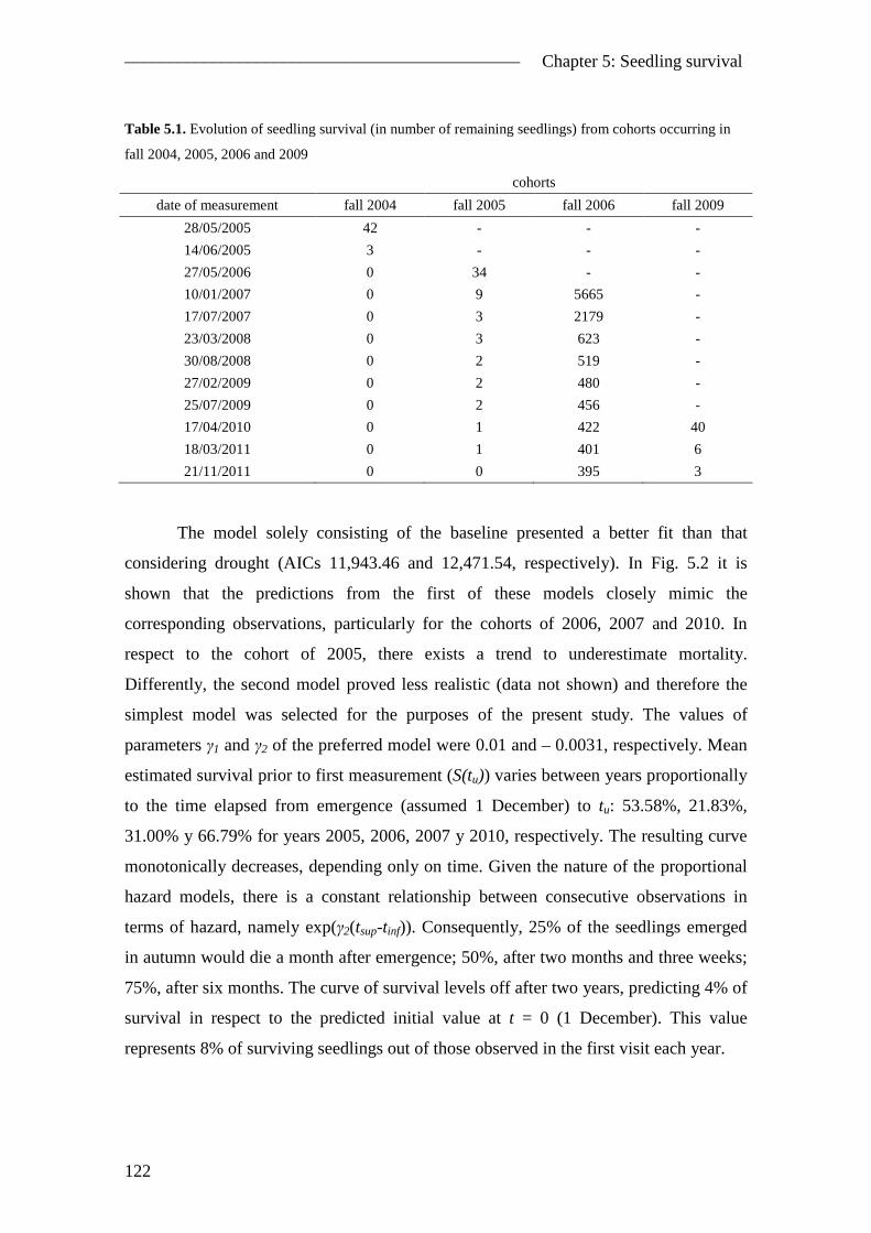
––––––––––––––––––––––––––––––––––––––––––––– Chapter 5: Seedling survival
122
Table 5.1. Evolution of seedling survival (in number of remaining seedlings) from cohorts occurring in
fall 2004, 2005, 2006 and 2009
cohorts
date of measurement fall 2004 fall 2005 fall 2006 fall 2009
28/05/2005 42 - - -
14/06/2005 3 - - -
27/05/2006 0 34 - -
10/01/2007 0 9 5665 -
17/07/2007 0 3 2179 -
23/03/2008 0 3 623 -
30/08/2008 0 2 519 -
27/02/2009 0 2 480 -
25/07/2009 0 2 456 -
17/04/2010 0 1 422 40
18/03/2011 0 1 401 6
21/11/2011 0 0 395 3
The model solely consisting of the baseline presented a better fit than that
considering drought (AICs 11,943.46 and 12,471.54, respectively). In Fig. 5.2 it is
shown that the predictions from the first of these models closely mimic the
corresponding observations, particularly for the cohorts of 2006, 2007 and 2010. In
respect to the cohort of 2005, there exists a trend to underestimate mortality.
Differently, the second model proved less realistic (data not shown) and therefore the
simplest model was selected for the purposes of the present study. The values of
parameters γ1 and γ2 of the preferred model were 0.01 and – 0.0031, respectively. Mean
estimated survival prior to first measurement (S(tu)) varies between years proportionally
to the time elapsed from emergence (assumed 1 December) to tu: 53.58%, 21.83%,
31.00% y 66.79% for years 2005, 2006, 2007 y 2010, respectively. The resulting curve
monotonically decreases, depending only on time. Given the nature of the proportional
hazard models, there is a constant relationship between consecutive observations in
terms of hazard, namely exp(γ2(tsup-tinf)). Consequently, 25% of the seedlings emerged
in autumn would die a month after emergence; 50%, after two months and three weeks;
75%, after six months. The curve of survival levels off after two years, predicting 4% of
survival in respect to the predicted initial value at t = 0 (1 December). This value
represents 8% of surviving seedlings out of those observed in the first visit each year.

––––––––––––––––––––––––––––––––––––––––––––– Chapter 5: Seedling survival
123
.
0 500 1500 2500
0.0
0.2
0.4
0.6
0.8
1.0
days from 01-Dic-2004
surv
ival
S(tu)
0 500 1000 1500 2000
0.0
0.2
0.4
0.6
0.8
1.0
days from 01-Dic-2005
surv
ival
S(tu)
0 500 1000 1500
0.2
0.4
0.6
0.8
1.0
days from 01-Dic-2006
surv
ival
S(tu)
0 200 400 600
0.0
0.2
0.4
0.6
0.8
1.0
days from 01-Dic-2009
surv
ival
S(tu)
5.5. Discussion
The model presented in the current study precisely predicts seedling survival of
P. pinea for those cohorts emerged in fall as a function of seedling age.
Despite being only few, a fraction of the seedlings originated in fall finally
became established. The successfully establishment of these recruits contrasts with the
almost total mortality of the seedlings emerged in spring. This fact indicates that
summer drought is a strong limiting factor for recruitment for just-emerged seedlings,
such as suggested by Calama et al. (2012). On the contrary, and according to the results
from our models, drought appears not to affect those seedlings that had already faced
the winter period. This feature informs a relevant ecological adaptation of P. pinea to
xeric environments, in contrast to other pine species in the Mediterranean, where severe
summer droughts lead to the complete destruction of two-years-old cohorts (Tíscar-
Oliver, 2007). From a spatial perspective, other factors, such as the influence of
overstory, needs to be tested in the future. In this respect, the medium shade-tolerant
behaviour exhibited by P. pinea (Awada et al., 2003) suggests a better performance of
seedlings when relatively high stand densities are present, as demonstrated for other
Mediterranean shade-tolerant species (i.e. Pinus nigra; Ordóñez et al. (2004)) and
already pointed out for P. pinea by Calama et al. (2012).
Figure 5.2. Observed
(circles) and predicted
(crosses) seedling survival
over time for the four used
cohorts. The horizontal line
represents the estimated
survival up to time of
cohort detection (S(tu)).
The vertical line stands for
the instant tu. Note that
observations have been
scaled so that they coincide
with predictions at tu

––––––––––––––––––––––––––––––––––––––––––––– Chapter 5: Seedling survival
124
All processes involved in regeneration of P. pinea are partially responsible for
regeneration failure through either low transition probabilities between consecutive
stages or the occurrence of a bottleneck (Calama et al., 2011; Manso et al., 2012b;
Manso et al., 2012c; in press; Manso et al., 2012d). Along with this circumstance, the
observed high mortality rates suggest that current intensive and strict regeneration
fellings (Montero et al., 2008) severely condition recruitment, as cuttings are commonly
conducted before seedlings could be considered as established. In this respect,
flexibility is needed in the application of fellings.
In a context of climatic change, where summer droughts are thought to increase
(De Castro et al., 2005), more difficulties to successfully achieve natural regeneration in
the Mediterranean are expected (Valladares et al., 2005). Consequently, the impact of
more drastic and persistent droughts on seedlings emerged in fall may be relevant. The
extent at which this circumstance will affect natural regeneration should be study in
detail, given the dramatic consequences for the persistence of the species.

––––––––––––––––––––––––––––––––––––––––––––– Chapter 5: Seedling survival
125
References
Awada, T., Radoglou, K., Fotelli, M. N. & Constantinidou, H. I. A. (2003) Ecophysiology of seedlings of three Mediterranean pine species in contrasting light regimes. Tree Physiology, 23, 33-41.
Blondel, J. & Aronson, J. (1999) Biology and wildlife of the Mediterranean region. Oxford University Press, Nueva York.
Calama, R., Cañadas, N. & Montero, G. (2003) Inter-regional variability in site index models for even-aged stands of stone pine (Pinus pinea L.) in Spain. Annals of Forest Science, 60, 259-269.
Calama, R., Madrigal, G., Manso, R., Garriga, E., Gordo, F. J. & Pardos, M. (2012) Germinación, emergencia y supervivencia de regenerado en Pinus pinea L. La regeneración natural de los pinares en los arenales de la Meseta Castellana (eds J. Gordo, R. Calama, M. Pardos, F. Bravo & G. Montero). Instituto Universitario de Investigación en Gestión Forestal Sostenible (Universidad de Valladolid-INIA), Valladolid.
Calama, R. & Montero, G. (2007) Cone and seed production from stone pine (Pinus pinea L.) stands in Central Range (Spain). European Journal of Forest Research, 126, 23-35.
Calama, R., Mutke, S., Tomé, J., Gordo, J., Montero, G. & Tomé, M. (2011) Modelling spatial and temporal variability in a zero-inflated variable: The case of stone pine (Pinus pinea L.) cone production. Ecological Modelling, 222, 606-618.
De Castro, M., Martín-Vide, J. & Alonso, S. (2005) The climate of Spain: past, present and scenarios for the 21st century. A preliminary assessment of the impacts in Spain due to the effects of climate change. ECCE Project-Final report, pp. 1-64. Ministerio de Medio Ambiente, Madrid.
Lawless, J. F. (2003) Statistical Models and Methods for Lifetime Data. Wiley Series in Probability and Statistics, pp. 630. Wiley & Sons, New Jersey.
Manso, R., Calama, R., Madrigal, G., Garriga, E., De Blas, S., Gordo, F. J. & Pardos, M. (2012b) Dispersión primaria, dispersión secundaria y predación post-dispersión en Pinus pinea L. La regeneración natural de los pinares en los arenales de la Meseta Castellana (eds J. Gordo, R. Calama, M. Pardos, F. Bravo & G. Montero), pp. 254. Instituto Universitario de Investigación en Gestión Forestal Sostenible (Universidad de Valladolid-INIA), Valladolid.
Manso, R., Fortin, M., Calama, R. & Pardos, M. (2012c) Modelling seed germination in forest tree species through survival analysis. The Pinus pinea L. case study. Forest Ecology and Management, in press.
Manso, R., Pardos, M., Keyes, C. R. & Calama, R. (2012d) Modelling the spatio-temporal pattern of primary dispersal in stone pine (Pinus pinea L.) stands in the Northern Plateau (Spain). Ecological Modelling, 226, 11-21.
Montero, G., Calama, R. & Ruiz Peinado, R. (2008) Selvicultura de Pinus pinea L. Compendio de Selvicultura de Especies (eds G. Montero, R. Serrada & J. Reque), pp. 431-470. INIA - Fundación Conde del Valle de Salazar, Madrid.
Ordóñez, J. L., Franco, S. & Retana, J. (2004) Limitation of the recruitment of Pinus nigra subsp. salzmanii in a gradient of post-fire environmental conditions. Ecoscience 11, 296-304.
R Core Team (2011) R: A language and environment for statistical computing. R Foundation for Statistical Computing, Vienna, Austria.
Selander, J. (1993) Survival model for Pinus sylvestris seedlings at risk from Hylobius abietis. Scandinavian Journal of Forest Research, 8, 66-72.

––––––––––––––––––––––––––––––––––––––––––––– Chapter 5: Seedling survival
126
Thornthwaite, C. W. & Mather, J. R. (1957) Instructions and tables for computing potential evapotranspiration and the water balances. Climatology 10, 181-311.
Tíscar-Oliver, P. A. (2007) Dinámica de regeneración de Pinus nigra subsp. salzmannii al sur de su área de distribución: etapas, procesos y factores implicados. Investigacion Agraria-Sistemas y Recursos Forestales, 16, 124-135.
Valladares, F., Peñuelas, J. & de Luis, E. (2005) Impacts on terrestrial ecosystems. A preliminary assessment of the impacts in Spain due to the effects of climate change. ECCE Project-Final report. Ministerio de Medio Ambiente, Madrid.

Chapter 6 Multistage stochastic model
6. Multistage stochastic model
6. Multistage stochastic model


Based on:
Manso, R., Pukkala, R., Pardos, M., Miina, J. & Calama, R. (Unpublished data) A multistage stochastic regeneration model for Pinus pinea L in the Northern Plateau (Spain), in preparation.
Specific objective:
7.- Formulating the integral model, from where (i) different silviculture alternatives can
be evaluated under varying climatic scenarios; and (ii) the optimal schedule for
regeneration fellings can be found out
Data:
- Outputs from (i) models based on those developed in Chapters 2, 3, 4 and 5 of the
present dissertation and (ii) cone production model by Calama et al. (2011)
Methodology:
- Multistage stochastic model
- Stochastic simulation
- Stochastic spatial optimisation
Main findings and management implications:
- Multistage stochastic regeneration models are a suitable tool for simulating
regeneration performance under different silviculture alternatives and climatic
scenarios; also, they permit to optimise management in regard to regeneration success
- Current stand densities at rotation age are insufficient to guarantee adequate dispersal,
the optimal value being around 150 stems·ha-1. Rotation length needs to be extended up
to 120 years
- In addition, flexibility is required in the scheduling of the regeneration fellings, which
could comprise even longer regeneration periods
- In consequence, P. pinea regeneration dynamics in unmanaged stands may lead to
uneven-aged structures
- Under a scenario of climatic change, P. pinea shows an acceptable behaviour
concerning natural regeneration, which reveals a notable ecological value of this species
to be considered in the future

––––––––––––––––––––––––––––––––––––– Chapter 6: Multistage stochastic model
131
6. Multistage stochastic model
6.1. Abstract
Natural regeneration represents an essential factor in sustainable forest
management. Pinus pinea L. woodlands located in the Northern Plateau of Spain have
been object of modern management for over a century but, unfortunately, natural
regeneration has not always been successful. Regeneration has not thrived either under
the seed-tree system or under the shelterwood system without complementary seeding.
Moreover, serious concerns arise in the perspective of a changing future climate. In
order to quantify recruitment under different silviculture alternatives and varying
climatic scenarios, and to optimise management scheduling, a stochastic multistage
regeneration model is presented. The model consists of a multiplicative structure where
each factor represents the transition probability between the different stages, from seed
production to definitive seedling establishment. Outputs of a seed production submodel
are therefore multiplied by the transition probabilities assessed through the submodels
of dispersal, germination, post-dispersal seed predation and seedling survival. All
submodels include stand and climatic variables. Model simulations show that current
stand densities at rotation age are insufficient to guarantee adequate dispersal, the
optimal value being around 150 stems·ha-1. Identically, rotation length needs to be
extended up to 120 years, in order to benefit from higher per tree seed production.
These results are confirmed by the stochastic optimisation, which additionally suggests
that more flexible regeneration felling schedules are needed to achieve natural
regeneration in the species. This fact may indicate that P. pinea would spontaneously
grow in semi-uneven-aged stands, accordingly to its medium shade-tolerant behaviour.
Regeneration performance does not appear to worsen under a scenario of climate
change, as long as relatively high rotation lengths and stand densities are permitted.
This acceptable behaviour under climatic change conditions informs an additional
ecological value for the species in Mediterranean sites threatened by an increasingly
severe drought occurrence.
Keywords: natural regeneration, transitional probability, stochastic spatial optimisation,
climatic change

––––––––––––––––––––––––––––––––––––– Chapter 6: Multistage stochastic model
132
6.2. Introduction
Natural regeneration in forest species has been modelled from two main
perspectives. A first approach consists of the so called recruitment models. They predict
the abundance or occurrence of established seedlings directly from environmental,
climatic or silvicultural explanatory variables (e.g. Eerikäinen et al., 2007; Fortin and
DeBlois, 2007; Barbeito et al., 2011). Thus, the response variable aggregates all
previous processes relevant for establishment. Recruitment models are simple but show
limitations when the mechanisms involved in regeneration at subprocess level (e.g. seed
production, dispersal, etc.) require special attention (Price et al., 2001). This is the case
of critical variables affecting only a single stage in the process during a short time
interval and that could be unnoticed when modelling regeneration marginally. Also,
when bottlenecks at some stages are expected, recruitment models may prove
inadequate.
Multistage regeneration models constitute an alternative approach to overcome
these shortcomings (e.g. Leak, 1968; Ferguson et al., 1986; Pukkala and Kolström,
1992; Ordóñez et al., 2006). This approach considers regeneration as a multistage
process consisting of underlying consecutive subprocesses that usually can be identified
as a series of successive survival thresholds for potential seedlings (Pukkala and
Kolström, 1992). Therefore, the probability of regeneration occurrence in space and
time can be seen as the product of the transition probabilities corresponding to each
involved sequential subprocess. Consequently, multistage models are, at least partly,
process-based models, presenting mechanistic basis at subprocess level. In multistage
models transition probabilities are separately assessed. They can be empirically
obtained, being unique for a specific subprocess (Rey and Alcántara, 2000) or
exhibiting a discrete number of values corresponding to different possible states of a
particular phase (Ordóñez et al., 2006). A more complex but rather more flexible
possibility is to model each transition probability as a set of explanatory variables.
Moreover, from a management standpoint, it is convenient to include climatic and
silvicultural variables among the explanatory variables.
Regardless of the modelling approach, regeneration models can be used
deterministically (i.e. model response produces an unequivocal output) or stochastically
(i.e. model response is subject to random variability inherent to the process). The

––––––––––––––––––––––––––––––––––––– Chapter 6: Multistage stochastic model
133
numerous sources of uncertainty arising from the subprocesses involved in regeneration
often render deterministic models insufficient for management purposes. Hence, the use
of stochastic models is essential to produce accurate and unbiased predictions (Miina
and Heinonen, 2008).
This background was taken into account when we undertook the effort of
modelling natural regeneration in Pinus pinea L. in the Northern Plateau of Spain, a
particularly complicated case of unsuccessful regeneration in managed forests. P. pinea
is an essential species in Mediterranean ecosystems, often occupying sites where few
tree species are able to thrive due to the typical Mediterranean weather conditions,
continental winters and sandy soils. In addition, the species provides important
economic benefits to local populations from its timber and edible seed production.
There are over 50,000 ha of managed P. pinea forest on the Northern Plateau. Natural
regeneration in these forests is rarely successful when using the existing regeneration
methods and this situation may worsen under future climate scenarios in Spain (De
Castro et al., 2005). To date, several studies have focused on the modelling of the
different stages of natural regeneration in P. pinea (seed production (Calama et al.,
2011); seed dispersal (Manso et al., 2012d); germination (Manso et al., 2012c; in press);
seed predation (Manso et al., 2012b) and seedling mortality (Manso et al., 2012a; in
press)), concluding that all these subprocesses can potentially become a bottleneck for
regeneration. However, the challenge remained to ensemble this information into an
integral model for the species.
In order to accomplish this task, a multistage stochastic model was developed.
Transition probabilities were independently modelled, based on the aforementioned
partial studies for the species, through climatic, environmental and silvicultural
variables. This model formulation is particularly useful as it makes possible to conduct
predictions in order to evaluate the effect on regeneration of different climatic scenarios
and varying silvicultural alternatives at spatial and temporal level. In this respect, the
model can be used as a complement of the growth and yield simulator PINEA2 (Calama
et al., 2007). So far, we are not aware of any multistage regeneration model comprising
these options. In addition, the model was implemented in an optimisation routine
addressed to find out the management schedule that maximizes the probability of
uniform recruitment occurrence. Although optimisation has been widely used in forestry
studies to maximize the production of different resources (Valsta, 1992; Hyytiäinen and
––––––––––––––––––––––––––––––––––––– Chapter 6: Multistage stochastic model
134
Tahvonen, 2002; González-Olabarría et al., 2008; Pasalodos-Tato et al., 2010), to our
knowledge the target has never been natural regeneration.
The main aims of this study were (i) to evaluate suitability of different
silviculture alternatives in regard to natural regeneration under different climatic
scenarios in P. pinea even-aged stands in the Northern Plateau of Spain; and (ii) to
optimise the regeneration fellings schedule. For these purposes, a multistage stochastic
regeneration model for the species was developed. Our prior hypotheses to be tested
from the resulting simulations and optimisations are that (i) more flexible management
schedules would be the key aspect to successfully achieve natural regeneration in the
species; and (ii) future climate may negatively impact on natural regeneration, although
adequate management schemes could mitigate these effects.
6.3. Material and methods
6.3.1. Regeneration model
In the present study, seed dispersal, seed germination, post-dispersal seed
predation and seedling survival were considered as transitional subprocesses with
transition probabilities Pdij, Pgij, Ppij and Psij, respectively, for the location i in the time
j. In the case of dispersal, the probability of a seed to reach the given location i in the
time j needs to be summed over all trees k expected to disperse to location i. The
product of these probabilities times the number of seeds Nkl produced by the tree k in the
year l represents the complete sequence of the regeneration process. Therefore, the
generic expression for the number of established seedlings for the location i in the time j
= 1 would be:
( ) 11111 1 iiikik
kli PsPpPgPdNS ⋅−⋅⋅⋅=∑ [6.1]
It can be easily followed that the generalized equation for any time j yields:
( ) ( ) ijijijk
ijijkklijij PsPpPgNPdNSS ⋅
−⋅⋅+⋅+= ∑ −− 111 [6.2]
The submodels explaining the transitional probabilities considered in the present
paper are briefly detailed below. Given the temporal precision of the submodels, a
monthly time step was set for the regeneration model.
––––––––––––––––––––––––––––––––––––– Chapter 6: Multistage stochastic model
135
Seed production
Based on Calama et al. (2011), this submodel provides annual predictions of
seed production at tree level. The original model was formulated as a zero-inflated
lognormal linear mixed model, meaning that: (i) it predicts the probability of a given
tree to bear cones in a specific year through a binomial process, considering the species’
masting habit; (ii) conditional to cone occurrence, lognormal predictions on cone weight
per tree for that year are provided. The weight of cones for a given tree was transformed
into our interest variable Nkl (seeds·(year·tree)-1) using the dimensional correction
deduced by Morales (2009). Covariates accounting for cone occurrence and cone weight
are of four types: tree variables, stand variables, site variables and climatic variables. In
this respect, different factors can limit seed production, including (i) too low or too high
densities, which could lead either to seed limitation or to a reduction in the per tree cone
production, respectively (Calama et al., 2008b; Calama et al., 2011); (ii) tree age, as the
younger the individual, the lower the production, up to an age of 120 years; and (iii)
intense dry conditions and extreme frost events affecting the key periods of cone
formation, which gives rise to P. pinea masting habit (Mutke et al., 2005a; Calama et
al., 2011) .
Dispersal
The spatial pattern of dispersal of P. pinea seeds was parameterized by Manso et
al. (2012d) based on the 2Dt model developed by Clark et al. (1999a). In this submodel,
Pdik is defined through the kernel, or Poisson-distributed probability of a seed from a
particular tree k to drop in a specific location i. The kernel is a monotonic decreasing
function of the distance between the tree k and the considered point i. Thus, the number
of seeds Nikl from tree k reaching the location i during year l would be the product of the
kernel Pdik and the nut production of tree k for that year Nkl. The total number of seeds
expected in point i is assessed as the sum of Njk over all trees. Providing year k is a mast
year, low values of Pdik are due to stand densities below a certain threshold and/or a
highly aggregated pattern of adult trees’ spatial distribution, resulting in dispersal
limitation, given the very short dispersal distance characteristic of P. pinea (Barbeito et
al., 2008; Manso et al., 2012d)
The submodel accounting for the temporal pattern of seed release in P. pinea is
detailed in Manso et al. (2012d). Once a suitable thermal threshold for cones to open is

––––––––––––––––––––––––––––––––––––– Chapter 6: Multistage stochastic model
136
reached (mean monthly temperature>16 ºC), the model produces monthly predictions
on the proportion of released seeds out of those remaining in the cone in the previous
month. This proportion is a linear function of the square root of total monthly
precipitation.
Germination
The utilised germination submodel was that proposed by Manso et al. (2012c; in
press). In the mentioned study, germination modelling in P. pinea was approached
through a proportional-hazards mixed model. The probability Pgij of a seed to germinate
in a specific time interval j at location i can be interpreted as a binomial process and it is
predicted on a daily basis via integration of the hazard function. This function describes
the daily germination rate conditional to no prior emergence. The hazard function was
defined as the product of a generic germination baseline and several nonlinear functions
of covariates ranging from zero to one. Covariates controlling germination were
climatic (thermal) and stand-related (overstory influence). An additive autoregressive
term was included in the model to deal with daily correlation in the hazard. The model
takes into account the interval and right censoring nature of observations as well as the
lack of independence within years through the inclusion of random effects affecting the
baseline. From this submodel it can be inferred that at temporal level, germination is
favoured by occurrence of adequate –though rare– thermal conditions in fall and it is
limited by frost events, the optimal period for germination being limited to few days in
late fall and spring. Moreover, occasional dispersal to large enough overstory gaps can
motivate Pgij to significantly decrease (Manso et al., 2012c; in press).
Predation
The seed predation submodel used in the current study is based on that described
in Manso et al. (2012b), producing monthly predictions of predation probability Ppij for
P. pinea seeds. As zero records (no seed survival due to predation) occurred in more
units than expected from the correspondent distribution, it was assumed that two
different mechanisms affected the probability of seed predation: occurrence of absolute
predation in a given location and abundance of survival conditional to no absolute
predation. Abundance was considered binomial-distributed, as it can be assumed that all
seeds hold the same probability of being predated, providing they have not been
destroyed before. The aforementioned features were accommodated through a zero-
––––––––––––––––––––––––––––––––––––– Chapter 6: Multistage stochastic model
137
inflated binomial linear mixed model, considering data correlation within years. The
covariates accounting for both mechanisms described the main environmental trophic
characteristics that control predator population: water availability (system primary
productivity) and food inputs, independent of current weather (P. pinea masting habit).
Only predation by rodents is considered, as seed losses caused by birds can be assumed
as negligible (Manso et al., 2012b). According to this model, the safe period for seeds is
restricted to summer months, coinciding with dispersal in the species. Therefore, seed
predation becomes a conditional bottleneck: whenever fall germination fails, most
dispersed seeds will be destroyed due to total winter exploitation. This effect is partially
mitigated along with increasing seed production.
Seedling survival
In order to consider mortality of emerged seedlings in the regeneration process,
a simplification of the model developed by Manso et al. (2012a; in press) was
employed. The daily probability Psj of a seedling to survive is predicted through a
proportional-hazards regression model. In this model, the hazard function was assumed
to be a Weibull mortality baseline affected uniquely by the age of the seedling, thus
daily mortality rate decreases monotically over time. This model predicts high mortality
rates of seedlings during the first year since emergence, strongly limiting recruitment in
the species. Therefore, only a few individuals from abundant cohorts that resulted from
favourable conditions in all previous phases (fruit production, dispersal, germination
and predation) are likely to persist.
Given the multiplicative structure of our model, regeneration failure will be
motivated by the existence of a bottleneck in at least one of the considered sequential
subprocesses. As the explanatory variables included in the corresponding submodels
account for both, stand structure and climatic features, bottlenecks must be due to (i) the
spatial arrangement and age of mother trees; and to (ii) the occurrence of adverse
climatic conditions. A summary of the covariates included in all models as well as their
influence in the correspondent subprocess is shown in Table 6.1.
Further information on experimental design and data collection can be found in
the referred literature and the previous chapters of this dissertation.

––––––––––––––––––––––––––––––––––––– Chapter 6: Multistage stochastic model
138
Table 6.1. Description of the used models
model submodel level covariates effect random effect time lag
cone production occurrence stand log(Na) – plot year
tree db/dgc +
site SId +
NUe categorical
temporal ppf (may to jun 3ybd) +
(climate) pp (oct to nov 3ybd) +
frostg (dec to mar) –
abundance stand log(N) –
tree d +
d/dg +
site SI +
NU categorical
temporal pp (may to jun 3ybd) +
(climate) pp (oct to nov 3ybd) +
pp (jul to sep 2ybd) +
pp (feb to may) +
frost (dec to mar) –
dispersal (spatial) - stand distance to trees – - -
tree seed production +
dispersal (temp) - temporal pp + - month
(climate) thermal cut-off +
germination - stand IPOTh + year day
temporal max temperature optimal
(climate) time from last frost +
- autorregressive term +
predation non-occurrence temporal drought – year month
(climate) cumularive pp 3mbp +
abundance stand seed production +
temporal drought +
(climate) cumularive pp 3mbp –
seedling survival - - time + - day aN: stand density; bd: dbh; cdg: mean squared dbh; dSI:site index; eNU:natural unit; fpp: precipitation (ybd: years
before dispersal; mbp: months before predation); gfrost: number of days with severe frost; hIPOT: influence potential (competition index)
6.3.2. Stochastic simulation
In order to evaluate the effect of management on recruitment, the described
model was used to simulate natural regeneration for different silviculture alternatives.
Specifically, the influence on regeneration of varying stand stockings and rotation
lengths existing at the beginning of the regeneration period was tested during an interval
of 10 years. In order to achieve realistic results on final recruitment, mortality was
––––––––––––––––––––––––––––––––––––– Chapter 6: Multistage stochastic model
139
allowed to occur for an additional 10-years period, according to predictions from the
weather-independent survival submodel. Moreover, provided that a majority of the
subprocesses are climate-mediated, these simulations were conducted both under
current climatic conditions and also considering the predictions for central Spain in the
last third of the 21st century under the A2 climate-change scenario (De Castro et al.,
2005).
As a starting point, deterministic stands holding typical conditions of the end of
the rotation within the range of application of all submodels have to be defined to
compute simulations in. To accomplish this task, we simulated twelve 100 m × 100 m
plots where tree location was the result of a Poisson process. A buffer strip of 12 m was
also taken into account. Single tree development was simulated using the growth
module of the software PINEA2 projecting up to an age of 80, 100 and 120 years an
initial common 20-years-old even-aged P. pinea stand with 500 stems·ha-1 and site
index 15 m. Besides rotation length age, simulated plots differed in the applied thinning
schedule, which led to densities at rotation age of 50, 100, 150 and 200 stems·ha-1,
resulting in twelve age-density combinations.
The regeneration process was stochastically simulated at each of the twelve plots
using scenarios (Rockafellar and Wets, 1987; Valsta, 1992) by means of the software
RODAL 5.0 (Pukkala, 2003�2012). Each scenario consisted of a joint realization of the
stochastic processes involved in the model over the planning horizon. Simulation under
many scenarios will provide a weighted outcome to be used to generate a probability
regeneration map for the plot. Therefore, for each of our twelve initial, deterministic
plots, 500 simulations (corresponding to one scenario each) were computed at 1 m2
scale. As a result, 500 regeneration Boolean maps were generated where those 1 m2
quadrats where at least one seedling was predicted to establish were assigned the value
of one. Otherwise, a zero value was given. Finally, the average value over the 500 maps
for each quadrat was calculated, producing as a result a regeneration map where each
cell value ranges from zero to one, representing the mean probability of holding at least
one seedling at the end of the regeneration period. Additionally, the average probability
µ across all 1 m2-quadrats of the resulting regeneration map and the standard deviation σ
of the probability among all cells in the same map were assessed.
The stochastic scenarios to be simulated were defined as follows:
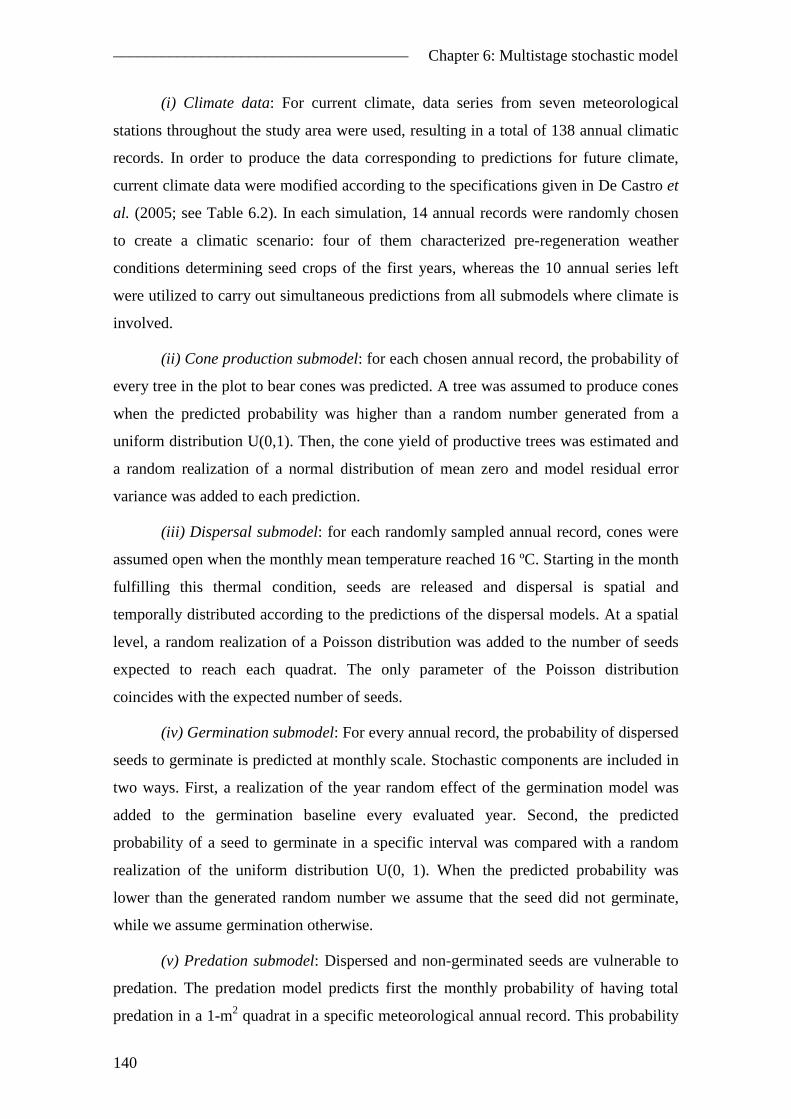
––––––––––––––––––––––––––––––––––––– Chapter 6: Multistage stochastic model
140
(i) Climate data: For current climate, data series from seven meteorological
stations throughout the study area were used, resulting in a total of 138 annual climatic
records. In order to produce the data corresponding to predictions for future climate,
current climate data were modified according to the specifications given in De Castro et
al. (2005; see Table 6.2). In each simulation, 14 annual records were randomly chosen
to create a climatic scenario: four of them characterized pre-regeneration weather
conditions determining seed crops of the first years, whereas the 10 annual series left
were utilized to carry out simultaneous predictions from all submodels where climate is
involved.
(ii) Cone production submodel: for each chosen annual record, the probability of
every tree in the plot to bear cones was predicted. A tree was assumed to produce cones
when the predicted probability was higher than a random number generated from a
uniform distribution U(0,1). Then, the cone yield of productive trees was estimated and
a random realization of a normal distribution of mean zero and model residual error
variance was added to each prediction.
(iii) Dispersal submodel: for each randomly sampled annual record, cones were
assumed open when the monthly mean temperature reached 16 ºC. Starting in the month
fulfilling this thermal condition, seeds are released and dispersal is spatial and
temporally distributed according to the predictions of the dispersal models. At a spatial
level, a random realization of a Poisson distribution was added to the number of seeds
expected to reach each quadrat. The only parameter of the Poisson distribution
coincides with the expected number of seeds.
(iv) Germination submodel: For every annual record, the probability of dispersed
seeds to germinate is predicted at monthly scale. Stochastic components are included in
two ways. First, a realization of the year random effect of the germination model was
added to the germination baseline every evaluated year. Second, the predicted
probability of a seed to germinate in a specific interval was compared with a random
realization of the uniform distribution U(0, 1). When the predicted probability was
lower than the generated random number we assume that the seed did not germinate,
while we assume germination otherwise.
(v) Predation submodel: Dispersed and non-germinated seeds are vulnerable to
predation. The predation model predicts first the monthly probability of having total
predation in a 1-m2 quadrat in a specific meteorological annual record. This probability
––––––––––––––––––––––––––––––––––––– Chapter 6: Multistage stochastic model
141
was compared with a random number sampled from the uniform distribution and total
predation was predicted to occur if the probability value was higher than the random
realization. Conditional to quadrat-level survival, probability of seed-level survival
during that month was predicted and randomized through the same procedure, given its
binomial nature. An additional source of stochasticity is given by the year random effect
affecting both processes within the model. As the estimated covariance of both random
components is non-null, randomization cannot be carried out directly from uncorrelated
random numbers generation. Therefore, Cholesky decomposition of the variance-
covariance matrix of the year effects was calculated and then multiplied by a 2 × 1
matrix whose rows represented uncorrelated random realizations from two normal
distributions of mean zero and variances equalling one. The two values of the resulting
matrix were used as correlated year effects in both parts of the model.
(vi) Seedling survival submodel: the number of seedlings from different monthly
cohorts was reduced uniformly across quadrats over time accordingly to the climate-
independent predictions from the survival submodel. No randomization was carried out
in this model.
Table 6.2. Changes in mean temperature (ºC) and total precipitation (%) under the A2 climatic scenario
in Central Iberian Peninsula in the last third of the 21st century
Dec to Feb Mar to May Jun to Aug Sep to Nov
temperature + 3.7 + 4.6 + 5.9 + 4.9
precipitation – 21.6 – 40.8 – 48.7 – 26.2
6.3.3. Stochastic optimisation
Besides evaluating the impact of the silviculture applied through the cycle on
regeneration via simulations, the regeneration felling scheduling can be optimised in
order to maximize sufficient and well distributed recruitment for a given stand.
Initial stand
A 250-stems·ha-1 stand with a bimodal diameter distribution was simulated.
Diameter distribution resulted from the mixture of two normal distributions of mean 20
and 40 cm and standard deviation 3 and 7 cm, respectively. Two thirds of the diameters
were sampled from the first distribution whereas the rest were randomly selected from
the second one. Lower diameters were assigned to those trees standing in denser
positions. The coordinates of 80 trees were generated by a Poisson process. Subsequent

––––––––––––––––––––––––––––––––––––– Chapter 6: Multistage stochastic model
142
tree locations were identically simulated, but the position was only retained when the
distance to the closest tree was lesser than a random realization of a Weibull distribution
(shape parameter = scale parameter = 1), leading to an aggregated distribution of trees.
Objective function
A function to maximize representing the interest of managers concerning natural
regeneration is to be defined. Successful regeneration is expected to be abundant and
evenly distributed. These two features were summarized in this study through the
following objective function (OF):
( )σµ −+= 1OF [6.3]
µ and σ being defined in subsection 6.3.2. Higher values of µ imply in general
better average conditions for regeneration in the stand whereas lower values of σ
indicate a more even distribution of seedling throughout the considered space.
Decision variables
A management schedule is defined by a set of controllable variables, called
decision variables. Optimisation of decision variables leads to an optimum management
schedule that, in the case of this study, maximizes the probability of abundant and
uniform natural regeneration. The chosen decision variables determined the felling
intensity during the regeneration period and the sequence in which trees are removed in
fellings. The sequence depended on the size and spatial distributions of trees. Decision
variables were chosen so as to take into account main stand conditions affecting
regeneration. The tree-selection algorithm developed by Pukkala et al. (1998) and
modified for optimisation purposes by Pukkala and Miina (1998) was adopted. When
using the original algorithm, less competitive trees are removed first. The
aforementioned modification includes two parameters b1 and b2 that are optimised along
with the rest of decision variables. The effect of these parameters is to provide a high
degree of flexibility in felling tree-selection, which in turn makes it possible to
accommodate the optimal spatial organisation of tree diameter in regard to regeneration.
The number of fellings (Nfell) was not optimised but a feasible schedule was set
consisting of two operations taking place in the first and fifth year of the regeneration
period, respectively (Nfell = 2). As a conclusion, in the present optimisation problem
decision variables were felling intensity (in percentage of removed trees) and

––––––––––––––––––––––––––––––––––––– Chapter 6: Multistage stochastic model
143
parameters b1 and b2 at each intermediate harvest operation, which yields 3 × Nfell
decision variables.
Optimisation method
The optimisation algorithm utilised in this problem was the direct search method
of Hooke and Jeeves (1961). This method does not require the use of derivatives and
therefore is appropriate for non-smooth and non-differentiable objective functions. It
consists of two differentiated steps: exploratory search and pattern search. From a user-
defined starting base point, the exploratory search alternately looks for the best solution
in the direction of the coordinate axes by altering one decision variable at a time. This
procedure basically provides a direction defined by the original base point and the best
solution found by exploratory search. Then, pattern search moves the base point along
this new direction and the process is repeated again. The step size is reduced when the
search does not find a better solution in the next move, so that convergence is assumed
to occur when step size is lower than a certain proportion (0.001 in this study) of the
initial step size for all decision variables. Each search-move implies a call to the
simulator, which evaluates the value of the objective function with the information
provided by the optimiser based on 500 scenarios. In order to test the effect of using
different starting points, optimisation was initialized from two different base points,
defined by two sets of decision variables. The first of them corresponds to a light
management (intensity of fellings of 10% and 20%, respectively; b1 = 1 and b2 = 2). The
second starting point was set to be representative of intensive management (intensity of
fellings of 70% and 50%; b1 = – 1 and b2 = – 2). The optimisation was assessed through
the software RODAL 5.0.
6.4. Results
6.4.1. Stochastic simulations
Effect of stand structure
The mean probability of holding at least one seedling·m-2 (µ) increased after a
10-years period along with both stand final density and rotation age (Figs. 6.1 and 6.3a).
The increment in µ was lower as the tested densities became larger, with a tendency to
level off when density was higher than 150 stems·ha-1. This pattern was similar for all
rotation ages, whose effect was basically to evenly intensify the effect of density in all

––––––––––––––––––––––––––––––––––––– Chapter 6: Multistage stochastic model
144
situations. µ values averaged 0.50 for the 50 stems·ha-1 plot, 0.74 for the 100 stems·ha-1
plot, 0.82 for the 150 stems·ha-1 plot and 0.85 for the 200 stems·ha-1 plot, across rotation
ages.
Concerning the degree of uniformity of established seedlings’ spatial
distribution, measured by the standard deviation of the quadrat-level probability of
holding at least one seedling·m-2 (σ), there was a trend to decline as density increased.
However, no clear pattern arose in regard to rotation age. σ values started to level off at
densities as high as 150 stems·ha-1. Mean values of σ across rotation ages were 0.23 in
the 50 stems·ha-1 simulations, 0.11 in the 100 stems·ha-1 simulations, 0.06 in the 150
stems·ha-1 simulations and 0.06 for the 200 stems·ha-1 simulations.
Effect of climate
Simulations under the A2 climatic scenario revealed that climate change would
presumably influence natural regeneration of P. pinea. The effect of future climate is
mainly evidenced through a gradient of increment of µ values in respect to those
predicted for the current climate along with decreasing densities and increasing rotation
ages. In the opposite extreme of this tendency, simulations carried out considering
rotations of 80 and 100 years and densities over 50 stems·ha-1 showed an reduction in
terms of µ (Table 6.3; Figs. 6.2 and 6.3b). Overall, µ reached maximum values of 0.74
and 0.82 when simulating 80 and 100 year rotations, respectively, as the leveling off
was appreciable at densities as low as 100 stems·ha-1 and the tendency of µ was even to
decrease beyond 150 stems·ha-1. On the contrary, for the longest rotation, µ exceeded
0.90 at the highest stocking. Contrastingly, σ values presented little changes under the
A2 climatic scenario.
Table 6.3. Proportion of variation in predicted mean probability of establishment between the A2 climate
scenario and current climate for different densities and rotation lengths. Negative values represent
decreasing future probabilities and positive values stand for increasing future probabilities
density (stems·ha-1)
Rotation (yr) 50 100 150 200
80 0.145 – 0.033 – 0.029 – 0.113
100 0.124 0.052 – 0.003 – 0.079
120 0.112 0.056 0.015 0.027

––––––––––––––––––––––––––––––––––––– Chapter 6: Multistage stochastic model
145
Figure 6.1. Maps of the simulated probabilities of achieving at least one established seedling at 1 m2
scale in 100 m × 100 m plots at the end of the regeneration period for varying densities and rotations
under current climatic conditions. Dark colours indicate lower probability whereas light colours stand for
higher probability. Circle positions represent tree locations and circle size is proportional to tree’s dbh. µ
and σ are, respectively, the mean and standard deviation of the probability among 1 m2 quadrats. OF = µ
+ (1 – σ)

––––––––––––––––––––––––––––––––––––– Chapter 6: Multistage stochastic model
146
Figure 6.2. Maps of the simulated probabilities of achieving at least one established seedling at 1 m2
scale in 100 m × 100 m plots at the end of the regeneration period for varying densities and rotations
under predicted climatic conditions in the A2 scenario. Circle positions represent tree locations and circle
size is proportional to tree’s dbh. Dark colours indicate lower probability whereas light colours stand for
higher probability. µ and σ are, respectively, the mean and standard deviation of the probability among 1
m2 quadrats. OF = µ + (1–σ)
––––––––––––––––––––––––––––––––––––– Chapter 6: Multistage stochastic model
147
Figure 6.3. Mean (µ, higher lines) and standard deviation (σ, lower lines) probability of establishment for
varying densities and rotations (dotted line, 120 years; slashed line, 100 years; solid line, 80 years) under
current (a) and future (b; A2 scenario) conditions
6.4.2. Optimisation
The optimisation algorithm converged regardless of the defined starting point.
Convergence criterion was reached for the base point representing light management
when the objective function was OF = 1.6608 (µ = 0.8250, σ = 0.1642). This maximum
of the objective function corresponds to the decision variables’ optimal solution
consisting of fellings intensity of 30.16% and 18.75%, for the first and second felling,
respectively, and b1 = 1 and b2 = 4, implying that small trees are to be removed from
dense places. Concerning the second starting point, the maximized value of the
objective function was OF = 1.6298 (µ = 0.7998, σ = 0.1700), which implied intensity
fellings of 20.00% and 12.50%, respectively, and b1 = 1 and b2 = 0.75, as the optimal
solution. In both cases the optimal scheme for achieving natural regeneration included a
slight reduction of the stand initial density and an even less intensive second felling,
both of them removing thinner trees located in the densest areas (Figs. 6.4 and 6.5). The
progress of the objective function and the decision variables over the iterative process is
shown in Fig. 6.6. The provided light-management initial solution resulted to be a close-
to-optimal solution, as the search in the surroundings of the given values for the
decision variables did not seemingly produce a substantial improvement in the objective
function. Only intensity of the first felling and the b2 parameter changed to some extent
from the starting point, rapidly stabilizing after the first moves of the direct search. In

––––––––––––––––––––––––––––––––––––– Chapter 6: Multistage stochastic model
148
contrast, when started from the intensive-management solution, the algorithm spent up
to 20 iterations before the objective function leveled off, the initial values of decision
variables being noticeably modified.
Figure 6.4. Optimised order of tree
logging for the optimisation initialized
from close-to-optimal initial values. In
(a), circle sizes represent the logging
order (larger circles are to be cut first); in
(b) and (c) circle sizes are proportional
to tree’s dbh and darker circles stand for
the logged trees in the first and second
harvest operation respectively
Figure 6.5. Optimised order of tree
logging for the optimisation initialized
from sub-optimal initial values. In (a),
circle sizes represent the logging order
(larger circles are to be cut first); in (b)
and (c) circle sizes are proportional to
tree’s dbh and darker circles stand for
the logged trees in the first and second
harvest operation respectively

––––––––––––––––––––––––––––––––––––– Chapter 6: Multistage stochastic model
149
Figure 6.6. Evolution of the utility function (OF) and decision variables (felling intensities and
parameters b1 and b2) through iterations in the optimisation initialized from close-to-optimal (left) and the
optimisation initialized from sub-optimal values of decision variables (right)

––––––––––––––––––––––––––––––––––––– Chapter 6: Multistage stochastic model
150
6.5. Discussion
In the current study we presented a multistage stochastic model for natural
regeneration in P. pinea. There are two main aspects contributing to the originality of
this paper. On the one hand, the key environmental and climatic effects and the random
variability associated to each subprocess were thoroughly defined and modelled. This
model specification (i) renders the estimation of the transition probabilities highly
flexible across a continuous range of relevant ecological inputs and (ii) enables
simulations of seedling establishment under different climatic scenarios and
management alternatives. On the other hand, the further implementation of an
optimisation algorithm based on the model represents a novel tool for decision making
in managed P. pinea stands.
6.5.1. Stochastic simulations and stochastic optimisation
Model simulations suggested that stand densities below 150 stems·ha-1 at the
beginning of the regeneration period may be suboptimal for attaining an adequate
number of emerged seedlings in a 10 years period (i.e. high µ), mainly due to dispersal
limitation and seed shortage. Identically, stockings above the aforementioned value do
not appear to improve µ, revealing the effect of declining cone production at high stand
densities (Calama et al., 2011). In contrast, σ only noticeably changed over varying
stockings (the higher density, the lower σ; Fig. 6.3a and 6.3b). In the light of these
results, µ seems to be strongly dependent on factors driving seed production and
dispersal, whereas σ is only closely related to the spatial arrangement of parent trees.
This fact is also observed when considering the effect of rotation length, which only
affects µ: shorter rotations (i.e. 80 years) would reduce µ due to seed limitation as
younger trees are less productive (Calama et al., 2011).
The best results for natural regeneration, considering only a 10 years interval,
are attained for the highest rotation tested (120 years; µ = 0.89, σ = 0.04), when the
optimal stand density is met (150 stems·ha-1). In spite of not being straightforwardly
comparable due to dimensional incompatibility, these results largely improve the
records from manager inventories under current felling schedules, where seedling
density was below 200 seedlings·ha-1 in 44% of the surveyed area and only in 10% it
was over 1,600 seedlings·ha-1 (Gordo et al., 2012).

––––––––––––––––––––––––––––––––––––– Chapter 6: Multistage stochastic model
151
The abovementioned finding of an optimal stand density of 150 stems·ha-1 is
confirmed by the outputs resulting from the first and second optimisation, where the
programmed fellings at algorithm convergence reduced the initial density (250 stems·ha-
1) in 39% and 32.5% of the stems in 5 years, respectively. Moreover, from a spatial
perspective, final b1 and b2 values indicate that fellings should be addressed to remove
first those trees of lower diameter from denser areas. Seed production and dispersal
subprocesses mainly drive this circumstance. On the one hand, smaller trees are
potentially less productive and account for a decrease in the per tree productivity at
stand level (Calama et al., 2011); hence, they are to be cut rapidly. On the other hand,
trees located in open areas are preferred to remain, even if low productive, given the
short dispersal distances of the species (Manso et al., 2012d), as the final seedling
distribution should be as uniform as possible. Accordingly, in optimisation problems
where the per tree value is not relevant, resulting b1 and b2 usually lead to the removal of
large trees first, as in Pukkala and Miina (1998).
The two different starting points led to final management schedules qualitatively
equivalent, although not exactly the same. The reason behind this fact is that the used
algorithm does not necessarily converge to the global maximum (Miina, 1998). There
are two particularities in this study case that potentially can hamper the finding of this
absolute maximum. On the one hand, the remarkable degree of stochasticity involved in
the regeneration process implies that every call to the simulator may result in highly
varying values of the objective function, even for identical values of the decision
variables. This drawback was counteracted by using a high number of simulations in
each call. On the other hand, estimated transition probabilities are generally positively
related to stand density. Therefore, several combinations of felling intensity may lead to
similar final values for the objective function, as long as the cuttings are light enough to
just cancel out the unfavourable effect of over-dense stands in seed production. The
same applies for b1 and b2 parameters: given that few subprocesses are controlled by
spatial covariates, only the positive effect of age (dbh) on seed production and the
clustered distribution of dispersal can inform the parameters’ value.
The objective function used in the present optimisation problem combines two
features of interest for regeneration: the mean (µ) and the standard deviation of (σ) of
the probability of regeneration for a given plot at 1 m2 precision. Although these two
variables are obviously correlated, none of them can be neglected. Whereas very high

––––––––––––––––––––––––––––––––––––– Chapter 6: Multistage stochastic model
152
values of µ will lead unequivocally σ to be null, lower µ are possible under different
spatial distribution of seedlings (varying σ), some of them being more adequate than
others. Nevertheless, caution must be taken when using this objective function below
realistic stand densities and spatial arrangement. The relationship between µ and σ is not
monotonic for the full domain of the two variables. However, this relation was found to
be always decreasing within the range used in the present study (µ over 0.35).
6.5.2. Current implications for management
Current management in P. pinea in the study area primary focuses in pine nut
production. Consequently, stands reach the regeneration period with very low densities
ranging from 80 to 125 stems·ha-1 at age 80–100 years. According to Montero et al.
(2008), the shelterwood method is then applied to regenerate the stands, consisting of
two highly intense fellings (50% reduction of the remaining trees) to be carried out
between the first and the 10th year of the regeneration period (preparatory felling and
seeding felling) and a final felling that extracts the few stems still standing in the 20th
year. This scheme strongly contrasts with the results of this paper for an adequate
management scheduling.
In fact, given that stand density in the beginning of the regeneration period is
normally below 150 stems·ha-1, no preparatory or even secondary fellings should be
conducted. Afterwards, the initial density should be maintained as long as needed, until
the occurrence of successful establishment events. Actually, first forest managers in the
region at the end of the 19th century were already aware of this circumstance (Romero,
1886). Despite the good results achieved in terms of number of recruits, problems were
detected concerning the viability of these saplings in the 1960s. These problems were
attributed to an excess of shade, promoting a –nowadays unsustainable– artificial
regeneration-based silviculture model, including strip clearcuttings (Gordo, 1999).
Indeed, seedlings need to be released from parent tree’s shade at some point, which
implies that a longer maintenance of relatively high stockings would not necessarily be
better for natural regeneration (Smith et al., 1996). However, the medium shade-tolerant
behaviour exhibited by P. pinea (Awada et al., 2003) suggests that seedlings can bear
relatively high stand densities at least during few years, these stockings favouring the
establishment of new recruits. Subsequently, parent trees should be progressively
removed to release from shade those cohorts with increasing light requirements. The
present multistage model does not include a seedling survival submodel taking into

––––––––––––––––––––––––––––––––––––– Chapter 6: Multistage stochastic model
153
account the effect of shade on long-term established seedlings. Further improvements in
this respect will make possible to optimise also the progressive removal of the
remaining trees as their role as a constraining factor for regeneration becomes more
important than those beneficial of seed source (Manso et al., 2012d) and shelter in the
first seedling stages (Calama et al., 2012).
Concerning rotation length, current values are also often below the proposed
optimal (120 years). Surprisingly, it is not uncommon that regeneration in managed
forests is perceived as unsuccessful due to too short rotation lengths (Tíscar-Oliver,
2007; Kerr et al., 2008). In these cases, if parent trees were allowed to remain longer
(increasing the length of the regeneration period), the probability of establishment will
increase, overcoming the effect of the various factors responsible for the reduction in
the transition probabilities or even the system’s collapse (bottleneck). Moreover, even
for optimal rotation lengths, the enormous stochasticity of the process and/or shorter
rotation lengths may lead to repeated failures over a longer time interval and therefore
flexibility will be needed to delay the planned cuttings after favourable regeneration
events. Identically, for those locations of very low quality, longer periods might be
required. A high degree of stochasticity in unfavourable conditions for regeneration was
also found for Mediterranean Pinus nigra by Tíscar-Oliver (2007), who concluded also
that flexible (discontinuous) fellings were required to guarantee successful recruitment.
As a consequence, if the regeneration period needs to be extended over 20 years in P.
pinea, a semi-even-aged stand structure would typically be expected. Interestingly, this
management schedule has been marginally attempted in the region for the species,
achieving reasonably good results (Finat et al., 2000).
Differently, from a spatial perspective, our results do coincide with current
silviculture practices. The present cone production-oriented management highlights the
importance of maintaining large trees as evenly distributed as possible, the condition
being fulfilled during the whole rotation through both thinnings and fellings (Montero
et al., 2008).
6.5.3. Future climate and future management
Interestingly, the application of the multistage model including simulated
climatic data for the A2 scenario did not reveal a worse performance of the system
concerning natural regeneration. On the contrary, the mean probability of establishment

––––––––––––––––––––––––––––––––––––– Chapter 6: Multistage stochastic model
154
increases in most tested circumstances. These findings can be explained in the light of
the specific impact of changing climate in the different climate-mediated subprocesses.
The first of them –seed production– is notably sensitive to precipitation reduction and
consequently fewer mast events and less abundant crops are expected. However, this
negative effect is clearly cancelled out or even reversed in the longest rotation and lower
densities by reduced seed predation: because rainfall is expected to decrease all over the
year, the predation-free period is to increase (Manso et al., 2012b). Consequently,
predation may be a less severe limiting factor, as seeds would be available to germinate
during a wider period. This pattern would be reinforced by the more drastic
precipitation decline taking place from July to August, which implies a negative lagged
response for rodent abundance in fall, the period where germination typically occurs.
Germination, however, is only thermal-mediated: on the one hand it is not negatively
affected by rainfall variations and, on the other hand, it is likely to be favoured by frost
decrease. Consequently, suitable conditions for germination would be both more
probable and extended longer.
The cases where probability of regeneration diminishes are those of higher
densities and shorter rotations. Given the definition of successful regeneration, it is
equally thriving to hold one seedling·m-2 than a higher quantity. Most probably, under
the current climate these plots contain a relevant number of quadrats successfully
regenerated but not far from the defined threshold. Considering seed production
reduction in the A2 scenario, it is most likely that a fraction of the stand comes in seed
limitation problems that in average are not compensated for by the increasing number of
successful seedlings right beneath the crowns.
As it has been showed, a sensible management of seed production (extending
rotation length) and dispersal (maintaining adequate stocking) can mitigate the impact
of climate change on the regeneration of P. pinea and even improve regeneration
performance in respect to current probabilities. Therefore, the same recommendations as
those stated for the current climate apply for the future: emphasis should be taken in
rotation age and scheduling flexibility. These measures are compatible with the general
recommendations for adaptive silviculture in Mediterranean forests in a context of
climatic change (Lindner et al., 2008). Whereas future conditions will promote
increasing growth in boreal and mountainous forests and therefore shortening of
rotation length will be a suitable adaptive measure (Kellomäki et al., 1997; García-

––––––––––––––––––––––––––––––––––––– Chapter 6: Multistage stochastic model
155
Gonzalo et al., 2007), the negative impact of drought on growth in the Mediterranean
suggests the opposite silviculture paradigm. Moreover, when silviculture techniques are
aimed to achieve the natural regeneration of stands, lowered rotations are generally
regarded as inadequate (Lindner et al., 2008). In respect to stand density,
recommendations to mitigate drought effects through evapotranspiration control and
increasing individual vigour point out to a more intensive thinning schedule, aimed to
reduce stand density (Kellomäki et al., 2000; Spiecker, 2003). Because management of
P. pinea woodlands is oriented to seed production, current stand density is among the
lowest in pine forests throughout Spain (Montero et al., 2008), meeting the
aforementioned proposal. Nevertheless, the conclusions from our study must be
considered prudently. At first, although precipitation reduction appears to be a
beneficial factor for natural regeneration, water shortage may also imply negative
effects on tree growth (Lindner et al., 2008). This circumstance indirectly affects
regeneration through seed production, modulating the effect of the different proposed
rotation lengths on natural regeneration. Secondly, the prey-predator system consists of
complex interactions (Kratina et al., 2009) and therefore predictions based on current
behaviour should not be deterministically admitted. Third, the effect of more intense
drought in seedling survival is unknown, although seedling performance is likely to
worsen (Valladares et al., 2005; Calama et al., 2012). Finally, future climate conditions
used in this study are the result of model predictions and therefore they are subject to
some degree of uncertainty (De Castro et al., 2005). Additionally, our results are
conditioned by the selected climatic scenario (A2; high emission increment). Would the
B2 scenario (moderate emissions increment) prove more realistic, our conclusions may
differ. In this respect, an advantage of the proposed stochastic model is that it considers
all feasible scenarios providing also multiple solutions for the different posed problems.
This is known as flexible adaptive planning and it has been stated to be an optimal
alternative among forest planning strategies (von Gadow, 2000). Furthermore, tools
such as that developed in the present paper are strongly encouraged by the European
Union Forest-Based Sector Technology Platform, which highlights the importance of
forest decision support systems (DSSs).
Overall, natural regeneration of P. pinea in the Northern Plateau of Spain
appears to be a reachable target, as long as management is adequate. In addition, the
acceptable behaviour exhibited by the species concerning natural regeneration in a

––––––––––––––––––––––––––––––––––––– Chapter 6: Multistage stochastic model
156
context of climate change, together with its frugal character, makes of P. pinea a
potentially resilient species of remarkable interest throughout different areas in Inner
Iberian Peninsula susceptible of aridification.

––––––––––––––––––––––––––––––––––––– Chapter 6: Multistage stochastic model
157
References
Awada, T., Radoglou, K., Fotelli, M. N. & Constantinidou, H. I. A. (2003) Ecophysiology of seedlings of three Mediterranean pine species in contrasting light regimes. Tree Physiology, 23, 33-41.
Barbeito, I., LeMay, V., Calama, R. & Canellas, I. (2011) Regeneration of Mediterranean Pinus sylvestris under two alternative shelterwood systems within a multiscale framework. Canadian Journal of Forest Research-Revue Canadienne De Recherche Forestiere, 41, 341-351.
Barbeito, I., Pardos, M., Calama, R. & Cañellas, I. (2008) Effect of stand structure on Stone pine (Pinus pinea L.) regeneration dynamics. Forestry, 81, 617-629.
Calama, R., Gordo, F. J., Mutke, S. & Montero, G. (2008b) An empirical ecological-type model for predicting stone pine (Pinus pinea L.) cone production in the Northern Plateau (Spain). Forest Ecology and Management, 255, 660-673.
Calama, R., Madrigal, G., Manso, R., Garriga, E., Gordo, F. J. & Pardos, M. (2012) Germinación, emergencia y supervivencia de regenerado en Pinus pinea L. La regeneración natural de los pinares en los arenales de la Meseta Castellana (eds J. Gordo, R. Calama, M. Pardos, F. Bravo & G. Montero). Instituto Universitario de Investigación en Gestión Forestal Sostenible (Universidad de Valladolid-INIA), Valladolid.
Calama, R., Mutke, S., Tomé, J., Gordo, J., Montero, G. & Tomé, M. (2011) Modelling spatial and temporal variability in a zero-inflated variable: The case of stone pine (Pinus pinea L.) cone production. Ecological Modelling, 222, 606-618.
Calama, R., Sánchez-González, M. & Montero, G. (2007) Integrated management models for Mediterranean multifunctional forests: the case of stone pine (Pinus pinea L.). EFI Proceedings.
Clark, J. S., Beckage, B., Camill, P., Cleveland, B., HilleRisLambers, J., Lichter, J., McLachlan, J., Mohan, J. & Wyckoff, P. (1999a) Interpreting recruitment limitation in forests. American Journal of Botany, 86, 1-16.
De Castro, M., Martín-Vide, J. & Alonso, S. (2005) The climate of Spain: past, present and scenarios for the 21st century. A preliminary assessment of the impacts in Spain due to the effects of climate change. ECCE Project-Final report, pp. 1-64. Ministerio de Medio Ambiente, Madrid.
Eerikäinen, K., Miina, J. & Valkonen, S. (2007) Models for the regeneration establishment and the development of established seedlings in uneven-aged, Norway spruce dominated forest stands of southern Finland. Forest Ecology and Management, 242, 444-461.
Ferguson, D. E., Stage, A. R. & Boyd, R. J. (1986) Predicting regeneration in the grand fir-cedar-hemlock ecosystem of the Northern Rocky Mountains. Forest Science, Monograph 26.
Finat, L., Campana, V. & Seseña, A. (2000) La ordenación por entresaca en las masas de piñonero de la provincia de Valladolid. I Simposio del pino piñonero (Pinus pinea L.) (ed J. d. C. y. León), pp. 147-157. Valladolid.
Fortin, M. & DeBlois, J. (2007) Modeling tree recruitment with zero-inflated models: The example of hardwood stands in southern Quebec, Canada. Forest Science, 53, 529-539.
García-Gonzalo, J., Peltola, H., Briceño-Elizondo, E. & Kellomäki, S. (2007) Effects of climate change and management on timber yield in boreal forests, with economic implications: A case study. Ecological Modelling, 209.
––––––––––––––––––––––––––––––––––––– Chapter 6: Multistage stochastic model
158
González-Olabarría, J. R., Palahí, M., Pukkala, T. & Trasobares, A. (2008) Optimising the management of Pinus nigra Arn. stands under endogenous risk of fire in Catalonia. Investigacion Agraria-Sistemas y Recursos Forestales, 17, 10-17.
Gordo, F. (1999) Ordenación y selvicultura de Pinus pinea L. en la provincia de Valladolid. Ciencias y técnicas forestales. 150 años de aportaciones de los ingenieros de montes (ed Fundación Conde del Valle de Salazar), pp. 638. Madrid.
Gordo, F. J., Rojo, L. I., Calama, R., Mutke, S., Martín, R. & García, M. (2012) Selvicultura de regeneración natural de Pinus pinea L. en montes públicos de la provincia de Valladolid. La regeneración natural de los pinares en los arenales de la Meseta Castellana (eds J. Gordo, R. Calama, M. Pardos, F. Bravo & G. Montero), pp. 254. Instituto Universitario de Investigación en Gestión Forestal Sostenible (Universidad de Valladolid-INIA), Valladolid.
Hooke, R. & Jeeves, T. A. (1961) "Direct search" solution of numerical and statistical problems. Journal of the Association for Computing Machinery, 8, 212-229.
Hyytiäinen, K. & Tahvonen, O. (2002) Economics of forest thinnings and rotation periods for Finnish conifer cultures. Scandinavian Journal of Forest Research, 17, 274-288.
Kellomäki, S., Karjalainen, T., Mohren, F. & Lapveteläinen, T. (2000) Expert assessment on the likely impacts of climate change on forests and forestry in Europe. European Forest Institute, Joensuu.
Kellomäki, S., Karjalainen, T. & Väisänen, H. (1997) More timber from boreal forests under changing climate? Forest Ecology and Management, 94, 195-208.
Kerr, G., Gosling, P., Morgan, G., Stokes, V., Cunningham, V. & Parratt, M. (2008) Seed production and seedling survival in a 50-year-old stand of Corsican pine (Pinus nigra subsp. laricio ) in southern Britain. Forestry, 81.
Kratina, P., Vos, M., Bateman, A. & Anholt, B. R. (2009) Functional responses modified by predator density. Oecologia, 159, 425-433.
Leak, W. D. (1968) Birch regeneration: a stochastic model. U. S. Forest Service Research NE-85.
Lindner, M., García-Gonzalo, J., Kolström, M., Green, T., Reguera, R., Maroschek, M., Seidl, R., Lexer, M. J., Netherer, S., Schopf, A., Kremer, A., Delzon, S., Barbati, A., Marchetti, M. & Corona, P. (2008) Impacts of climate change on European forests and options for adaptation. EFI-BOKU-INRA-IAFS, Joensuu.
Manso, R., Calama, R., Madrigal, G., Conde, M., Gordo, F. J. & Pardos, M. (2012a) Supervivencia del regenerado en Pinus pinea L. en la Meseta Norte. Previsiones en un contexto de cambio climático. V Reunión del Grupo de Trabajo de Selvicultura de la Sociedad Española de las Ciencias Forestales (SECF) "Regeneración natural y cambio global" (eds R. Ruiz-Peinado, J. Reque & R. Serrada). Sociedad Española de Ciencias Forestales, Madrid. in press.
Manso, R., Calama, R., Madrigal, G., Garriga, E., De Blas, S., Gordo, F. J. & Pardos, M. (2012b) Dispersión primaria, dispersión secundaria y predación post-dispersión en Pinus pinea L. La regeneración natural de los pinares en los arenales de la Meseta Castellana (eds J. Gordo, R. Calama, M. Pardos, F. Bravo & G. Montero), pp. 254. Instituto Universitario de Investigación en Gestión Forestal Sostenible (Universidad de Valladolid-INIA), Valladolid.
Manso, R., Fortin, M., Calama, R. & Pardos, M. (2012c) Modelling seed germination in forest tree species through survival analysis. The Pinus pinea L. case study. Forest Ecology and Management, in press.

––––––––––––––––––––––––––––––––––––– Chapter 6: Multistage stochastic model
159
Manso, R., Pardos, M., Keyes, C. R. & Calama, R. (2012d) Modelling the spatio-temporal pattern of primary dispersal in stone pine (Pinus pinea L.) stands in the Northern Plateau (Spain). Ecological Modelling, 226, 11-21.
Miina, J. (1998) Preparation of management models using simulation and optimisation. Tree seedling production and management of plantation forests (eds T. Pukkala & K. Eerikäinen), pp. 165-180. University of Joensuu. Faculty of Forestry, Joensuu.
Miina, J. & Heinonen, J. (2008) Stochastic simulation of forest regeneration establishment using a multilevel multivariate model. Forest Science, 54, 206-219.
Montero, G., Calama, R. & Ruiz Peinado, R. (2008) Selvicultura de Pinus pinea L. Compendio de Selvicultura de Especies (eds G. Montero, R. Serrada & J. Reque), pp. 431-470. INIA - Fundación Conde del Valle de Salazar, Madrid.
Morales, L. (2009) Modelos para la predicción del contenido y calidad de piñón en piñas de Pinus pinea L. en los valles del Tiétar y del Alberche. Master Thesis, Universidad Politécnica de Madrid, Madrid.
Mutke, S., Gordo, J. & Gil, L. (2005a) Variability of Mediterranean Stone pine cone production: Yield loss as response to climate change. Agricultural and Forest Meteorology, 132, 263-272.
Ordóñez, J. L., Molowny-Horas, R. & Retana, J. (2006) A model of the recruitment of Pinus nigra from unburned edges after large wildfires. Ecological Modelling, 197, 405-417.
Pasalodos-Tato, M., Pukkala, T. & Rojo Alboreca, A. (2010) Optimal management of Pinus pinaster in Galicia (Spain) under risk of fire. International Journal of Wildland Fire, 19, 937-948.
Price, D. T., Zimmermann, N. E., van der Meer, P. J., Lexer, M. J., Leadley, P., Jorritsma, I. T. M., Schaber, J., Clark, D. F., Lasch, P., McNulty, S., Wu, J. G. & Smith, B. (2001) Regeneration in gap models: Priority issues for studying forest responses to climate change. Climatic Change, 51, 475-508.
Pukkala, T. (2003�2012) RODAL 5.0: Simulation-optimisation system for the management of any-aged stands in Spain.
Pukkala, T. & Kolström, T. (1992) A stochastic spatial regeneration model for Pinus sylvestris. Scandinavian Journal of Forest Research, 7, 377-385.
Pukkala, T. & Miina, J. (1998) Tree-selection algorithms for optimizing thinning using a distance-dependent growth model. Canadian Journal of Forest Research-Revue Canadienne De Recherche Forestiere, 28, 693-702.
Pukkala, T., Miina, J., Kurttila, M. & Kolström, T. (1998) A spatial yield model for optimizing the thinning regime of mixed stands of Pinus sylvestris and Picea abies. Scandinavian Journal of Forest Research, 13, 31-42.
Rey, P. J. & Alcántara, J. M. (2000) Recruitment dynamics of a fleshy-fruited plant (Olea europaea): connecting patterns of seed dispersal to seedling establishment. Journal of Ecology, 88, 622-633.
Rockafellar, R. T. & Wets, R. J. B. (1987) Scenario and policy aggregation in optimization under uncertainty. IIASA Working Paper WP-87-119, Laxenburg, Austria.
Romero, F. (1886) El pino piñonero en la provincia de Valladolid. Imprenta y Librería Nacional y Extranjera de los Hijos de Rodríguez, Libreros de la Univesidad y del Instituto, Valladolid.
Smith, D., Larson, B., Kelty, J. & Ashton, P. (1996) The practice of silviculture: applied forest ecology. John Wiley & Sons, Inc., Hoboken.

––––––––––––––––––––––––––––––––––––– Chapter 6: Multistage stochastic model
160
Spiecker, H. (2003) Silvicultural management in maintaining biodiversity and resistance of forests in Europe Temperate zone. Journal of Environmental Management 67, 55-65.
Tíscar-Oliver, P. A. (2007) Dinámica de regeneración de Pinus nigra subsp. salzmannii al sur de su área de distribución: etapas, procesos y factores implicados. Investigacion Agraria-Sistemas y Recursos Forestales, 16, 124-135.
Valsta, L. T. (1992) A scenario approach to stochastic anticipatory optimization in stand management. Forest Science, 38, 430-447.
Valladares, F., Peñuelas, J. & de Luis, E. (2005) Impacts on terrestrial ecosystems. A preliminary assessment of the impacts in Spain due to the effects of climate change. ECCE Project-Final report. Ministerio de Medio Ambiente, Madrid.
von Gadow, K. (2000) Evaluating risk in forest planning models. Silva Fennica, 34.

Chapter 7 Conclusions
7. Conclusions


––––––––––––––––––––––––––––––––––––––––––––––––– Chapter 7: Conclusions
163
7. Conclusions
I. The spatial primary dispersal pattern of Pinus pinea proved strongly
aggregated, only 1% of the seeds being expected to drop beyond 2 crown radii.
Consequently, currently-applied regeneration fellings prevent seeds be to uniformly
dispersed throughout the stand. From a temporal perspective, seed release is climate-
controlled: cones break open when mean monthly temperature reaches a thermal
threshold (usually in May), whereas the subsequent release rate is positively related to
precipitation, taking place during the summer until early fall.
II. Germination of P. pinea seeds is governed by thermal and stand variables in
the Northern Plateau. On the one hand, the absence of climatic optimal conditions
severely limits the process, resulting in a narrow window for seed germination, which
occurs either in late fall or spring. On the other hand, extremely poor overstory cover
leads to low probabilities of germination. Additionally, there is a relevant time-lag
effect in the process, meaning that precedent environmental conditions significantly
influence current germination performance.
III. Apodemus sylvaticus is the main frugivour removing seeds of P. pinea,
whereas corvids affect seed crops to a much lesser extent. A. sylvaticus mainly acts as a
predator, exploiting almost all available seeds out of the dry period. The favourable
period for seed survival is a consequence of both the decreasing rodent populations due
to the effect of drought and the higher seed availability in summer, when dispersal takes
place. This fact suggests the existence of a dual climate prey-predator control, driven by
summer conditions and the climate-mediated masting habit of the species. From a
spatial perspective, seeds are more intensively predated in the close vicinity of trees and
potential shelters.
IV. The vast majority of emerged seedlings are expected to perish two years
after emergence. In the case of individuals from cohorts occurring in fall, a small
fraction can survive, the mortality rate being irrespective of any specific climatic event.
––––––––––––––––––––––––––––––––––––––––––––––––– Chapter 7: Conclusions
164
When considering those seedlings appeared in spring, none persists. Emergence rapidly
followed by severe summer drought could be behind this circumstance.
V. As it can be seen, all processes involved in natural regeneration of P. pinea
are subject to a high degree of uncertainty, including seed production, given the species
masting habit. This circumstance results in low transition probabilities between
consecutive stages or even leads to the collapse of the system (bottleneck). These
bottlenecks can occur as a consequence of dispersal limitation, high predation rates
before germination takes place, lack of suitable conditions for germination, and intense
mortality. However, an adequate management scheme can mitigate these difficulties.
VI. Simulations and optimisations undertaken through the developed multistage
stochastic model demonstrate that current intensive and strict regeneration fellings lead
to processes of dispersal limitation before a sufficient number of evenly distributed
recruits has been established. Longer rotation lengths, an optimal stand density at the
beginning of the regeneration period and more flexibility in the scheduling of
subsequent fellings are the key factors that would lead to successfully achieve natural
regeneration in even-aged stands of P. pinea in the Northern Plateau of Spain.
VII. According to model predictions, regeneration of P. pinea is expected to
show an acceptable behaviour in a context of a climatic change. In this respect, the
species proves highly valuable from an ecological point of view, as it will be able to
occur in demanding sites where other tree species probably will fail to persist.
VIII. The findings of the present dissertation indicate that, ideally, natural
regeneration of P. pinea would occur as follows: (i) seeds are dispersed in summer
during a mast event, mainly beneath parent tree’s crowns; as long as stand density is
high enough, no dispersal limitation should rise; (ii) seed germination thrives to take
place by early fall; (iii) seed predation diminished rates hold until emergence; (iv)
seedlings are then uniformly arranged in a sufficient number throughout the stand, so
that at least a surviving fraction of them definitely becomes established.

––––––––––––––––––––––––––––––––––––––––––––––––– Chapter 7: Conclusions
165
IX. Providing that parent tree’s crowns facilitate performance of established
seedlings for several years given the medium shade-tolerant behaviour of the species,
regeneration dynamics would rely on the regeneration under cover, until gaps in the
overstory occur. This feature and the characteristic low transition probabilities could
lead to various regeneration failures over time and therefore an uneven-aged stand
structure is expected.
X. Advanced statistical methods are required in order to precisely model the
subprocesses involved in natural regeneration, given the nature of data. Furthermore,
providing all subprocesses have been adequately modelled, the multistage stochastic
approach is a powerful approach to model the entire process of regeneration.
XI. Regardless of formulation complexity, the variables included in models
addressed to provide tools for forest management must be easily measurable/modifiable
by forest managers, such as climate and/or stand variables. This is the base of
silviculture and, consequently, the development of accurate but not accessible models
would be completely senseless.


Epílogo
Epílogo


–––––––––––––––––––––––––––––––––––––––––––––––––––––––––––– Epílogo
169
Epílogo
1. Motivación
El presente epílogo no es una sección de agradecimientos. Antes bien, se trata de una crónica de los últimos cuatro años de vida… o de agonía.
2. Caso práctico de modelización mediante análisis de supervivencia
La probabilidad de que el doctorando sobreviva como tal en el periodo en el que se desarrolla su tesis es un caso típico de aplicación de modelos basados en análisis de supervivencia. Si bien se puede definir una línea base de supervivencia que agrega un amplio abanico de variabilidad estocástica indefinida tal como la desidia, el aburrimiento o la desesperación, existen ciertas variables que aceleran o ralentizan el riesgo de que el doctorando lo mande todo a hacer puñetas.
Pero la supervivencia del sujeto está condicionada a la propia ocurrencia del proceso. Cuatro fueron las circunstancias que permitieron que el factor que define esta ocurrencia adoptara el valor de uno. En primer lugar, aunque ponerse con una tesis doctoral me sigue pareciendo que no es nada del otro barrio, lo cierto es que muy pocos “chicos de barrio” hacen tesis doctorales. Este mérito corresponde exclusivamente a mi casa (sin rodeos, el binomio padre-madre) que, sin seguramente saber muy bien cómo, han edificado sobre los escombros de un pasado en ruinas, común al de una generación de perdedores de guerras, una sólida estructura basada en el conocimiento, el esfuerzo y la dignidad. En segundo lugar, la actitud no sirve de nada si no se tiene acceso a la información sobre financiación para personal predoctoral. Imperativo es en este punto saludar a Salvia García y agradecerle el envío de esta convocatoria, demostrando que el apoyo mutuo es mucho más eficaz que la paralítica competencia. Como tercera condición en esta interacción a cuatro bandas se sitúa la osadía del salto al vacío: una vez dados todos los pasos hasta el borde del abismo, aún hay que atreverse a arrojarse. Mucha, mucha gente, tanta que no cabe aquí, escuchó mis dudas. De entre las personas que aún merecen que se les recuerde hay que destacar a aquellos zaragozanos/as de origen o de acogida como Belén Sirviente, Sergio Co!, Arantxa Lorente o David Gil “el Calata” y a alguna gente de la difunta EUIT Forestal como Alfredo Bravo y, una vez más, Valentín Gómez. Finalmente, cierran este grupo de elementos determinantes los, entonces, potenciales directores de tesis, Rafa Calama y Marta Pardos, que dieron un voto de confianza a una historia que podría no haber sido cierta (aunque lo era), creyendo seleccionar (digo yo) a un paradigma de la honestidad y “cráneo previlegiado”. Sólo se acercaron algo a la verdad en lo primero.
A partir de aquí, ya nadie regala nada. Entonces, ¿cómo definir la función de riesgo, esa tasa instantánea de “mortalidad de doctorando” cuya suma día a día nos permite evaluar el grado de frustración de aquél? La forma más sencilla es considerar de forma aditiva todas las variables influyentes y meterlas en una exponencial, acorde a la magnificación que de todo –dicen– hace el doctorando. Algunas de estas variables dependen del tiempo; otras no tanto. Estudiaremos la cuestión, en cualquier caso, considerando diferentes grupos de factores. Por otra parte, existe una parte de variabilidad que no podemos relacionar directamente con nada y que es intrínseca a distintos niveles. Es aquí donde se hace necesaria la inclusión de los efectos aleatorios: el efecto aleatorio despacho, el efecto aleatorio lo contentos que estén los jefes, el efecto aleatorio precio del café,. Los EBLUPs podemos asumir que son realizaciones aleatorias de una Normal, en el caso del precio del café-solo-con-hielo-para-llevar, de media 0.65€ y desviación típica 0.1€, de acuerdo al criterio de esa genial camarera llamada Tere.
3. Factores intrínsecos
En los comienzos, Rafa Calama, el cerebro de la Operación Pinea, tenía una idea de tesis que, retrospectivamente, vemos que respondía a un plan bien trazado, habida cuenta de que esa estructura sigue siendo la que sustenta el documento. Eso fue siempre una ventaja que amortiguó la caída de la probabilidad de supervivencia del doctorando antes mencionada: saber, sin fisuras, qué quedaba por hacer y a dónde queríamos llegar. La estructura de la que hablo, sin embargo, fue fuertemente zarandeada en esos primeros tiempos por el alto grado de entropía del entorno, hasta el ecuador de la beca, en el que Marta Pardos puso un poco de orden y se fijaron unos plazos que al final hemos ido
–––––––––––––––––––––––––––––––––––––––––––––––––––––––––––– Epílogo
170
cumpliendo. Entretanto, un factor positivo nada desdeñable fue el apoyo presupuestario para todo tipo de idas de pinza en relación a los experimentos vallisoletanos.
Como quiera que fuera muy rápido cuando yo lo empecé a percibir, cabe hablar ya del efecto INIA. El INIA tiene una envidiable disponibilidad de recursos, desde los coches a la reprografía, y de personal. Pero también tiene sus cosas, que terminan por afectar a la supervivencia del doctorando, de los contratados por el antiguo Régimen Especial Agrario en fraude o no de ley, del capataz, del tecnólogo, del investigador, y al mismo tiempo, son todos estos sujetos los que lo componen y lo retroalimentan. El efecto INIA en este sentido es semejante al bosón de Higgs: una especie de campo de ácido butírico y dimetil, en el que cada uno de nosotros no es sino una simple perturbación, parte integrante del mismo, como igualmente lo es este párrafo. Esperemos que, al contrario que el campo de Higgs, el efecto INIA no tenga vocación de eternidad y esté sujeto a cambios para bien.
Pero volvamos al resto de variables. Íbamos por los comienzos, cuando al llegar tempranito sólo se escuchaba, muy bajito, rock&roll en la radio de Estrella y la tos, menos bajito, del Kike. Las salidas de campo a tientas entre la niebla y los valores siempre negativos de la temperatura de la Tierra de Pinares se sucedían por entonces. Esto cambiaba cíclicamente según avanzaba el tiempo con episodios de insolación norteafricana. ¿Y aún alguien se preguntaba por qué el piñonero pasaba de regenerar por allí? Lo de acumular aproximadamente 12000 km en salidas de un día por allí arriba en su momento tuvo un impacto negativo. También para el pobre Guillermo Madrigal, cuando venía conmigo, que tenía que fingir durante horas lo muy interesado que estaba en mi imparable verborrea. En realidad, el problema de las salidas de campo no sólo correlaciona con el bosón de Higgs-INIA en forma de trámites, el tráfico de la A6 y con el clima, sino también con la preocupación de burlar como burlamos todos los controles de la Benemérita para poder meter en Madrid las dos fanegas de farlopa que siempre nos bajábamos de los pinares, así como las muchas “9 mm Parabellum” destinadas a reiniciar la lucha armada en Egoalde. En esto era especialista el bueno de Santi de Blas, más que yo si cabe, fiel aliado mío en muchas “excursiones” y en la lucha contra las alharacas de Valsaín. Siempre de signo positivo en este modelo de supervivencia, excepto el día que cruzó el Terrano en la pista aquella, el mismo día que se nos rajó una rueda. Un emocionado saludo desde aquí a aquel retén que nos sacó por dos veces del fango aquel día (aún estarán descojonándose, me imagino).
Positivo, igualmente, que Javier Gordo sea de los pocos gestores de Hispanistán que confía en la investigación. Y en consecuencia, también favorable el poder encontrarse de vez en cuando con los guardas de Tordesillas, Alejandro y Eugenio, ambos dos, antagonistas de los Romera. Eugenio, además, es un ecólogo de verdad, sin necesidad de publicar en revistas importantes ni saberse la última genialidad teórica de algún listo genérico al que todos nos toca citar. Disculparme desde estas líneas porque el dispositivo de predación aún debe andar descomponiéndose por sus propios medios en el pinar de la Nava. Los guardas, asimismo, echaron una mano con los datos cuando yo “andaba de vacaciones”, como se suele afirmar cuando estás en el extranjero trabajando como si no hubiera un mañana. En este sentido, gracias a la gente del INIA que anduvo al quite: Rafa, Guille y el personal de prácticas. Puntualmente también hasta se pringaron Carolina Mayoral, María Pasalodos (hauska tutustua, Marrrrria!) y Eduardo López, notable francófilo y frecuente consejero en asuntos morales y edáficos (gracias también a Salva por esto), con el que esperemos algún día podamos colaborar para aplicar mi amplia experiencia en el análisis de datos con exceso de ceros (sentimentales, sobre todo) a los falsos ceros en la ocurrencia de especies.
Otro efecto positivo, enlazando con lo anterior, es el de nuestra “plantilla flotante”, los famosos capataces en prácticas o cómo aprovechar(nos) del fraude de la formación. Aún a riesgo de olvidar a alguien: Sergio, Maribel, Susana, Paula, Rodri, Eduardo, Adrián y, especialmente Merche, mil gracias. Mar Conde, la más guapa del INIA y de Carabanchel Bajo, va aparte, aunque sólo sea por haber soportado más chapas que nadie en sus sucesivos contratos. Negativa, en cambio, la sensación de que este hecho esclavista no llega a entenderse como tal. Así nos va con eso de las conquistas sociales. Pero si de campo y de conquistas (de todo tipo) hablamos, ¿cómo obviar la función sinusoidal que describe mi buen amigo Enrique Garriga, el Kike? Cambiando una rueda, lijando rodajas, estudiando física, intoxicándose (conmigo) con la ración aquella de oreja en Mojados, escondiéndonos de los pelotazos de los antidisturbios en Tirso o vaciando un tercio de Mahou verde, un tipo siempre valiente, que si hace falta le mete “un rodamiento del 9 a la Secretaria General en el entrecejo”. Y no es broma. Pendiente queda el cochinillo y la botella de Ribera en Segovia, rediós.
En aquella primera fase forzosamente hay que hablar también de los cursos de doctorado, enfoque decididamente deficiente para la formación. No obstante, se trata del típico factor con diferentes niveles, algunos de ellos afectando de forma positiva a la variable respuesta. Entre estos debo resaltar a Miguel Ángel Ibáñez, de Agrónomos, Diseño de Experimentos, siempre dispuesto a

–––––––––––––––––––––––––––––––––––––––––––––––––––––––––––– Epílogo
171
ayudar en los cortocircuitos mentales de los alumnos sin el más mínimo interés por la estadística (sé que es aquí cuando queréis que hable de la Prêt. Pues no, os jodéis). Y a Carlos Morla, entrañable, en cuyo curso, además, tuve la ocasión de retomar el contacto con Raúl Iglesias, el Ruli, más conocido como el Sabio de Tubilla. Gloriosas jornadas del alpinismo-torocismo ibérico quedaron atrás empujadas por las suelas de nuestras botas. Primera mención especial para Sven Mutke, (“Eh’ben”, voz carpetana), quien me facilitó la bibliografía, me aconsejó y me revisó un trabajo infumable de historia medieval pinariega para uno de esos cursos, del que he tenido la deferencia para con los miembros del tribunal de sólo incluir algunas pinceladas en la introducción de esta tesis. Segunda mención especial: con qué poca gente se puede hablar de religiones ecológicas, sectas ácratas y otras minucias, con la seguridad de que además se está aprendiendo algo (y encima, en el bello castellano del siglo XVII). Tercera mención especial: remarcable excepción en las reuniones de grupo, levantando la mano para pedir la palabra; se nota el “background”, majo.
Por aquellos entonces también hubo un intento de transformación masiva a R, sospecho que con poco éxito. Aunque a Mathieu y a Rafa les rechinen los dientes yo voy a valorar positivamente que R exista, a pesar del bando dogmático que sustenta el sistema. Creo que Andrés Bravo estará conmigo.
Para terminar con la primera fase de la tesis, caracterizada por los palos de ciego contra la cabeza propia, particularmente con el tema de los bichos, hay que indicar que fue un elemento positivo la enorme amabilidad y disponibilidad de José Luis Tellería (Biología de la Complu) y Eduardo Mezquida (antes Montes Madrid, ahora en otros entornos más propicios, espero). No obstante, pese a las aportaciones de ambos, de María M. Jáuregui y de Alberto Hurtado (EUITF, aúpa), para mí, amigos, los bichos siguen siendo variables aleatorias y poco más.
Los “biodiversos” vinieron un poco después. La interacción con ellos (ellas, mayoría absoluta de chicas) a nivel laboral es poco significativa a causa de nuestras muy distintas orientaciones “pofesionales” del momento, pero debo incluirla en el modelo porque ahora me sabe francamente mal no haber aceptado nunca el cafelito y la magdalena que Marcelo amablemente me ofreció cada día. Ah, y porque los pantalones que le dieron a Laura me quedan increíblemente bien. Y aprovecho el momento histórico, aunque no pegue ni con cola, para mencionar que por ahí tuvo lugar el asalto al centro de una avanzadilla de la EUITF, Álvaro y Raquel.
Una interesante variable cuyo efecto mutó de positivo (por los vínculos) a negativo (por el seguimiento) según avanzaba el tiempo y que, por tanto, cabe introducir en nuestro modelo como una interacción cuadrática con aquél, es el de la (nada) famosa Asamblea de Becarixs. Mientras me entretenía pintando piñones, hecho objeto de mucha burla (englóbese en efecto Higgs-INIA), también perdíamos el tiempo principalmente Marina de Miguel, Quique Sáez y yo mismo (aunque en menor medida, también todos los de nuestra planta en el CIFOR y alguna gente “del otro lao”) en remitir un escrito al Director Particular (porque ya no era General) del INIA solicitando cinco tonterías de forma (paréntesis para Bea: siempre fuimos, somos y seremos; ¡salud!), en connivencia con Marisa Barragán, que siempre nos apoyó. Con la misma cintura con la que este Director Particular pasaba del escrito, el grueso de los becarios del INIA ignoraba, rechazaba y hasta despreciaba con alevosía hasta una raquítica hoja de firmas. Yo, que no soy rencoroso, les deseo todo lo mejor a esos esquiroles miserables con los numerosos artículos que habrán publicado mientras otros se preocupaban por su propia dignidad en el centro. Luis Alté estará de acuerdo conmigo, la única persona de por aquí que conoce el daño que hicieron los Pactos de la Moncloa.
Siguiendo esta línea, por lo que representa, por lo que le debemos, por lo que le admiramos, debo evaluar como variable aparte un fenómeno único en la naturaleza: JB. Estimado amigo, te dedico estas líneas. Aun con tu enorme parecido al Ministro De Guindos, éste no te llega ni a la suela en lo que se refiere a la defensa de los intereses del Estado. Serías un antidisturbios formidable, si dimensionalmente fuera posible. Te sugiero que leas el preámbulo de la Ley 30/1992, donde se indica para qué están los funcionarios públicos. Tampoco dejes de ojear el régimen sancionador. Eso de andar pidiendo barrenas de Pressler por el CIFOR para cargarte con sal un árbol colindante a tu parcela se llama malversación de fondos públicos. Y pobre árbol.
Menos mal que siempre estuvieron Dori y Toñi para evitar males mayores mediando con semejante individuo. Aparte, a mi modo de ver, estas dos mujeres ejemplares e infatigables en su capacidad administrativa son el verdadero motor del CIFOR. Su competencia, aliviar la parálisis que produce el entramado burocrático del centro y del INIA, así como su absurda rigidez, diríase de origen napoleónico. Curiosamente, me he encontrado Doris y Toñis en cada estancia. Creo que es el puesto más importante en un centro de investigación. Del mismo modo, aunque en general poca gente las considere compañeras de trabajo, y quizá por eso, debo incluir en este párrafo a quien hace que el

–––––––––––––––––––––––––––––––––––––––––––––––––––––––––––– Epílogo
172
CIFOR no sea un estercolero: Juani, por la que no pasan los años, e Isabel, que a pesar de los mismos, tiene diligencia para limpiar por las tardes, co-gestionar un bar por las mañanas y sacar adelante todas las plantas del centro.
Otro grupo de variables a considerar es aquél que engloba al resto de becarixs de selvicultura, que por proximidad, representan un colchón sobre el que recostar las miserias diarias y, por tanto, detienen la caída al vacío. Lástima que mi paso por el INIA ha sido en este sentido un poco como un paseo por las parameras de la Meseta Norte: al llegar yo, ya se iban Nacho Barbeito y Darío Martín, y ya se había ido Guillermo Gea. Me alegro sinceramente de la vuelta de este último, ¿o con quién podría yo discutir del verdadero significado de un mínimo relativo en la función de verosimilitud en un espacio n-dimensional sin llegar a la conclusión conjunta de que la ciencia es un negocio deshonesto y lamentable? Gente con tablas en cualquier caso.
Y por otra parte, las nuevas incorporaciones tardaron mucho en llegar para estar en el mismo momento del proceso de supervivencia. Los eché siempre en falta, incluso antes de saber que existían. Sin embargo, estos compañeros que dignamente recogen el testigo Pinea –Carolina Mayoral (experta musicóloga y envidiable “viviora” que estoy seguro debí ya haber conocido en el Crápula de Zgz) y Javier de Dios (¡un biólogo! ¿Será el principio del fin (por fin) de las masas puras DE forestales?)– son funciones de riesgo en sí mismas (para eso hacen la tesis a tiempo completo) que limitan el riesgo de mortalidad condicional del resto de doctorandos. Sin olvidar en este epígrafe, claro está, a Laura Fernández y Víctor Mora. Una pena que haya sido tan sorprendentemente complicado lo de compartir con ellos despacho, que es donde creo me correspondía.
Y, por cierto, a pesar de que los comienzos no les han sido del todo fáciles a ninguno, estoy seguro de que encontrarán su lugar en esto de la ciencia (también en el avispero) y que sus trabajos serán excelentes. Con la excepción del de Víctor, claro, que nos dio una admirable lección de humildad y creo que nos hizo a todos preguntarnos si esto merecía realmente la pena. Un tipo tremendamente válido, por lo demás, que no sólo jugaba bien al basket sino que en el fondo sabía de sobra por qué la inversa de la matriz hessiana de la función de verosimilitud es equivalente a la matriz de varianza-covarianza de los parámetros a estimar. Y es que el coincidir con gente más lista que uno mismo yo lo entiendo como una ventaja, no como una amenaza: el ingenio se lanza hacia delante y la eficacia se incrementa, superándose más rápido la fase de chapuza científica. En este sentido, la profesionalidad y la capacidad de computación tipo i-7 de Alicia Ledo, otra chica de barrio, son parte fundamental de la robustez de últimos pisos de esta tesis, aunque se discrepe en algo tan fundamental como es la preferencia de los empalagosos tintos de verano sobre un buen tercio de Mahou verde.
Y enlazando con eso de los últimos pasos del proceso, debo mencionar el interesante fenómeno (no muy positivo en esta formidable ecuación que propongo) que advertí según el entorno se iba oliendo que el final se acercaba: el ambiente súbitamente se torna todo paternalismo, paternalismo que recuerda a cuando el aguerrido ciclista pre-EPO, que se aferraba a su manillar para no caer al asfalto en el último y desesperado esfuerzo por coronar los Lagos de Covadonga, justo recibe la palmadita en el lomo de cientos de aficionados. Se agradece con sinceridad la atención, queridos, pero un punto de mesura, un punto de mesura…
Como vemos, son muchos los factores que afectan la supervivencia. La salud ha quedado hecha mierda en este periodo (cuánto se agradece que Rocío (Rotxi), mi compi de clase en el Gaudí, fuera tan determinada en escoger medicina y se convirtiera así en médico particular cuando a uno más lo necesita). Me pregunto si la tesis deja taras. Yo creo que sí: ahora soy peor persona. Me temo que algún día tenga que seguir las recomendaciones de José Pablo para ingresar en el centro de desintoxicación de Los Molinos.
4. Factores extrínsecos científicos
Las estancias. He aquí que el Ministerio a veces acierta, muy a pesar de JB. ¿Qué hubiera sido de esta tesis sin las estancias? Muy probablemente algo bien administrado pero no muy distante un puñado de pintones modelos mixtos generalizados. ¿Qué hubiera sido de la idea del doctorando sobre la investigación? El bosón de Higgs como teoría única. En suma, hubiera supuesto tasas tan elevadas de riesgo de perecer, que quizá hubieran catalizado un abandono definitivo del ámbito científico en algún momento.
La primera de les estadas va ser a Barcelona, Cerdanyola del Vallès, al Centre de Recerca Ecològica i Aplicacions Forestals (CREAF), amb en Josep Maria Espelta, en Tete, a qui vaig trobar un tio veritablement eficient, ordenat, professional i supersimpàtic. Tot i que va ser només d’un mes, vam
–––––––––––––––––––––––––––––––––––––––––––––––––––––––––––– Epílogo
173
aprofitar moltíssim, i no solament pel que fa de l’avanç a la tasca dels bichos, sino també per treballar des del punt de vista dels ecològs: cal n’aprendre molt! Tengo que agradecer también a José Luis Ordóñez el rato que echó conmigo para explicarme cómo iba el modelo estocástico de su tesis, porque fue así cómo entendí enteramente el objetivo de la mía. També he d’agrair el consells del Lluis Comas sobre els ratolins. A nivell personal, va ser un period força agradable amb en Tete, però també amb tota la gent del CREAF, particularmente con Roberto Molowny i el mon de becaris que hi havia. És bastant dificil oblidar-se’n, però és també complicat recordar tots els noms: el Guille, la Jara, Laura... Merci a tots per la vostra hospitalitat i molt especialment a la Lucia per fer més fàcil el camí cap a Montana.
En Barcelona vivía en Sans, gracias a los contactos talibanes movidos por la pequeña Soyarina. Allí compartía casa con el Nacho, el Popi, compañero castellanista y notable pensador que me hizo descubrir los bajos fondos barcelonís y los grifos de cerveza Voll-damn. Dentro de este bando de la casa estaba también Sawali, egipcio economista y abogado tetralingüe (árabe, inglés, francés y castellano) que trabajaba en un bar. Y el Manolín, que como si fuera de la casa. En el otro bando, el pulsar (hispano)navarro Laura-Lorea, del cual la primera llevaba la voz cantante. Nunca conseguimos que bajaran a Ciutat Vella a darle al alpiste.
També molt d’altres amics van contribuir a que l’estada fossi un èxit personal: moltes gràcies a la Marta i l’Andrea per fer-me sentir com a casa tot el temps. Mai podria jo haver pensat que la nit aquesta del partit del Barça fossi a acabar a aquella festa del copón al Gòtic (d’on, malauradament, es va escapar la Rosa de foc...) i d’allí, a la fi, a una casa modernista del Passeig de San Joan. Un plaer també sortir a la muntanyeta amb la Neus i el seu xicot, quedar amb en Dani-Alacant de Montes UPM, la Elena de Tarragona i de veure tan, tan bé a la Desireé. Espero que tot vagi igual ara...
The second stay was kind of exotic, in Missoula, University of Montana, with Chris Keyes. Chris was always a devoted host who did his best to make me feel as at home. And definitely, he succeeded. I strongly appreciate his efforts on our paper on dispersal. I think I improved quite a lot with scientific compositions in English at that time. Also I am sincerely grateful for the opportunity to travel with Tom (heart-breaker man!) to the forests of Mediterranean California as well as to the IMPRESSIVE sequoia forest at Reddish. Back in the lab, thanks also to David Affleck for solving my agonic doubts with R programming and to Bob Keane, from the Missoula Fire Lab for his interest in our work. Among the students, it was a pleasure to share room with Kyle, I’m sure nowadays a remarkable forester, and Woongsoon (sorry if the spelling is incorrect), a South Korean gay who can be listed among those who are intelligent beyond the average. Y como lo mío es juntarme con gente brillante, por ver si se pega algo, no podía ser de otra manera que llegara a trabar buena amistad con Adrienne Keller, brillantísima hispanófila “oregonesa”. Definitely, I like type-A people. Greetings also to my neighbours, Suyama, Helgue and his girlfriend, with whom I shared amazing beer-evenings. Y gracias, ante todo, a Juan Abarca, por crear y mantener en ese estado de pureza escatológica el virtuosismo de Mamá Ladilla, que me acompañó en cualquier momento de debilidad, estreñimiento o parálisis mental.
Però, és clar, cal parlar del Dani i la Margarita, dos fenómenos valencianets de la vida social missouliana, grands competidors en l’art de fer tortilles de patates. A més, si coneixes al Dani ja coneixes a tothom! I quina grand surpresa, quand va venir ca meva en Josep, ja conegut de un congress a Montpellier. Un tio excellent en Josep, critic i internacionaliste que, amb l’Albert (campion dels pedos!) i l’Anna, em van deixar un sitio al cotxe per poder anar a Yellowstone. Y en este contexto no podemos olvidar, por supuesto, a la Sole, (Soledad Jimena Inés, concretamente, no sé si ese era el orden), montañera patagónica excepcional. El Trapper Peak fue coser y cantar para nosotros tres and however we and the others would have found our death in the Missions but for the incredible sense of orientation of Charley. Hei, man, I still own you some pictures of the last hike we did! Finalment, he d’enviar una abraçada forta a l’Anna Sala, a la seva filla i al seu marit: estava collonut el pavo d’acció de gràcies!
Le troisième stage a été au centre INRA de Nancy (France). Je ne voulais pas. Je vraiment ne voulais pas. Mais il sembla que le destin avais fait un chemin unique, direction la Lorraine, bien difficile à ne pas le suivre. Je me suis aperçu à ça après voir, par hasard, un film de la Mélanie Laurent. En fait, j’étais bien sûr que je la rencontrerais sur Nancy. Pas de tout. Dommage. Mais par contre j’ai trouvé Mathieu Fortin. Ce n’est pas le même, mais de toute façon, je vraiment le dois beaucoup et on pourrait dire qui il y avait deux phases en la thèse: Before Mathieu et After Mathieu. Pour ce qui est de la statistique, pour ce qui est de la programmation, pour ce qui est de l’efficacité, pour ce qui est de la génialité, pour ce qui est de la capacité didactique et linguistique et sur tout, pour ce qui est de sa disponibilité.

–––––––––––––––––––––––––––––––––––––––––––––––––––––––––––– Epílogo
174
Et, en France, un autre mythe que tombe. Oui, semblant chez les catalans, les françaises, quand même les lorraines, sont des gens qui ne perdent pas le temps à penser comment enmerder les espagnols. Bientôt, tout le contraire, spécialement si on considère leur patience avec mon très déficient français. Comme exemple, les chercheurs de l’INRA, un d’entre eux me donnant même une bouteille de vin excellent ou les étudiants de la résidence de l’Engref: Matilde et beaucoup d’autres. Ou mes amis Tony (formidable cuisiner et magicien des eaux de vie), Haykel et Johannes (capable de pas mélanger le catalan, le castellan, le française et le português). Ou le groupe de stagiaires a l’INRA, particulièrement Vivien, palentino de acogida, como yo. Ou les très sympathiques filles du bus à Champenoux, avec particulier attention à la Leslie, jeune lorraine-alsacien qui toujours s’a excusé de boire une bière à cause de sa thèse (mis cojones 33). D’hors de l’environ INRA, ils ont été bien agréables avec moi Florent et Florence (brouillardé journée aux Vosgues!) et aussi Gabi. Et beaucoup plus loin du truc académique, il faut se rappeler à l’hospitalité de Coco et Sonja (¡no pasarán!). Y, por si fuera poco, hete ahí que coincidí en esta estancia con Marina, quien absorbió, como más cercana hispanoparlante, parte de la tensión que supone andar en dos artículos de lo mismo perfectamente a la par.
Ja Suomi! Rafa sanoi että täytyin mennä Joensuun. Ein halua mennä siellä uudelleen! Minusta Pöhjois-Karjala on liian kylmä ja seillä ei ola valo talvissa! Mutta Timo Pukkala ja Jari Miina olivat Joensuussa. And I wonder what kind of simulator I would have carried out and how long it would have taken without their selfless help, their deep knowledge on the underlying stochasticity of the processes to study, the formulation of such problems and, overall, their incredible capacity to solve any question, suggestion or shortcoming in a record time, regardless of the difficulty of the targeted objective. In this respect, I sincerely appreciate the confidence and rapid response of Jari to provide a favorable report for my thesis. Truly, this is optimization.
No menos increíble es la resiliencia del grupito español “finófilo” en Carelia del Norte. Y que a pesar del friazo de por allí, reciban con extraordinario calor a los viejos conocidos. Después del chiste tonto, debo pedir el aplauso más fuerte para uno de esos perpetuos hispano-fineses, Javier Arévalo, que me hizo la vida más fácil en todos los aspectos, integrándome en la farándula joensuusta y en las memorables pachangas de baloncesto del Metla. Asimismo, y por antigüedad, merece un hueco en este apartado el Jaume a qui no hi havia vist des d’una llunyana nit al Meksiko, ja fa sis anys. Y en otro orden de cosas, realmente agradable las charletas, cervezas y paseos con Isa (EUITF Madrid, dejando huella), Juha (Espanjalainen en el fondo), Sergio, Víctor, Antonio, Rubén, Javi Pasalodos y espero no olvidarme de nadie. En cualquier caso, quizá sea la maximización de las experiencias negativas, quizá sea este ambiente propicio, quizá sea el trabajar con gente seria, quizá sea esa luz boreal que no deja que el ánimo baje (ni dormir tampoco deja), quizá sea la Vía Carpetana pero la verdad es que la cuesta de Niinivaara nunca volvió a ser un obstáculo penoso para llegar a ese rincón del Pyhäselka llamado Hukanhauta.
Por cierto, que en Hukanhauta tenía dos compañeros finlandeses. Antti, carélico pura sangre, parco en palabras, digamos, pero un tío majo que creo que me tenía en buena estima. El death metal hace amigos. Y la tortilla de patatas y el salmón al horno, más. El otro, el Markus, en el fondo también me tenía aprecio, porque si no, no hubiera intentado evangelizarme con tanto ahínco.
And, concerning Finns, it was a pleasure to visit Tampere to meet Kapa and Adrien (français-finnois), one of the most expected encountering of all times. Sure there will be more, hopefully in the “warmness” of Lorraine! And to finish with Finnish people, it is compulsory, though the word may be inconsistent to some extent in this context, to identify the significantly positive effect of Johana and Jakko, representing the generational succession to JOA in Joensuu, in an effort for demonstrating that human beings only can be integrally free. Do not hesitate, it is always worthy to keep on.
Et un autre stage encore. Hors du temps de la thèse, mais reliée à la thèse de toute façon. Voilà que j’ai me rendu une autre foi en Nancy, pour finir quelques choses et développer une autre model avec des données de Rafa en suivant une autre idée brillante de Mathieu. Et c’est à ce moment-là quand j’ai intégralement eu le document intégrativement intégral de la thèse, comme François dirait. Tout ce que j’ai déjà dit sur Nancy est applicable ici, sauf que aussi on est allé à Freiburg, pour rencontrer Axel, le windthrow-modelling-man et le Valhala. También era diferente en Nancy que ahora la liebre ibérica, Nacho Barbeito, andaba, o más bien corría, por la Lorraine, a quien tengo que agradecer mi rapidísima reintegración en la localidad, los platos, los vasos y la tabla que luego se partió. Y también lo del segundo informe de experto que faltaba. La próxima St Georges será con entrenamientos más intensivos en la Pépinière. Se van a cagar los nancienses. No así los keniatas: el centro de África siempre corrió mejor que el norte del continente.

–––––––––––––––––––––––––––––––––––––––––––––––––––––––––––– Epílogo
175
A nosotros, por el contrario, nos visitó menos gente. Como interacciones significativas, mencionaré la de Luke, que estuvo a punto de morir de frío en el Ocejón, y la de César, que me recomendó el escribir unos agradecimientos orientados a objetos, pero programar las complejas interacciones de los elementos del bosón de Higgs-INIA está más allá de mis capacidades. Y aunque no se tratara de una estancia, por el tiempo que coincidimos, como si lo fuera: Ana Rincón, que resultó ser famosa por Nancy y que me dijo que le enviara el primer artículo tan pronto como saliera. El parto fue tan largo, que me olvidé.
Pero no sólo hubo estancias. También el Ministerio acierta con lo de los congresos, en general positivos en esta construcción estocástica de la supervivencia del doctorando.
El primero, el Congreso Forestal E’hhpañol de Ávila, buen sitio para pasearse y dejarse ver. Allí se coincidió con tanta gente que necesitaría un disco duro externo para acordarme, pero debo mencionar, al menos, al núcleo palentino, con Irene, Josu, Celia, Oli, etc., etc., a la Miriam Piqué, a Joserra, que me salvó el pellejo en Finlandia la primera vez, a Serrada, con el famoso símil de los pliegos y, en otro orden de cosas, a Pedro “el de Monflorite” y a Íñigo Oleagordia.
El segundo fue una cosa de la IUFRO en Palencia, donde ni que decir tiene que estaban los autóctonos dirigiendo. Me parece que fue aquí cuando Ricardo Ruíz-Peinado, pobre, debió flipar con “mi vida paralela” y los comentarios talibanes de mi amiga Ana, que suscribo íntegramente.
El tercer congreso fue en Francia, en Montpellier, una cosa de bichos y ecólogos. Aquí tengo que agradecerle a Rafa la búsqueda de financiación. Pensaba yo que el congreso no iba a tener relevancia para “lo nuestro”. Pero vaya que sí. Entre otras muchas cosas, supe que el queso francés es cojonudo, que Akiko Nakahasi era una chica de menos de 30 años, que a Kim V. le afectaba suficientemente “one point five bottles of white wine”, que Pedro Jordano es un tío llanísimo, que a Dani, el de Oviedo, espero encontrármelo otras muchas veces, que Carolina Puerta, quien me había dado amables consejos para la primera estancia, era de carne y hueso y que Juanjo Robledo Arnuncio es un verdadero crack que trabaja en el INIA.
La cuarta reunión fue la de transferencia del piñonero y el pináster en la capital financiera de Castilla, Pozal de Gallinas. Aunque fueron unas jornadas con regusto triste, creo que fueron a la vez una buena oportunidad para poner en práctica lo que, en mi opinión, debería ser un centro público de investigación y tecnología como el INIA: si enfocamos los recursos públicos sólo a sacar artículos sobre “trendy topics”, los verdaderos beneficiarios, gestores y sociedad, se van a terminar por mosquear. Además, fue un gusto reencontrarse con el núcleo palentino una vez más, escuchar la copla de Gregorio sobre el Caballero de Olmedo y asaltar la barra con el Kike (sí, fuimos nosotros).
La quinta fue una de la SECF, de modelización en Lugo. Creo que Mariola temió por su vida cuando me cortó el 40% de mi tiempo por orden de la superioridad dado que la Conselleira de Judías Pintas, Sardinas Arenques y Gusanos de Seda había llegado tarde al mitin de apertura. También tuvimos que escuchar algunas barbaridades sobre modelos mixtos contra las que Javier Vázquez y Rafa se batieron el cobre con el disgusto de entender que nadie ha terminado de entender nada después de 10 años de esto. Un requetegusto recoincidir por cuarta vez con el núcleo palentino y con la gente del CREAF. No tan agradable el discutir con mis ex-coincidentes laborales sobre cuáles son las normas tácitas que el doctorando asume al firmar su contrato. Me imagino que una vez reducido el sueldo un 11% y subidas las tasas un 100%, podemos dejar claro que aquí no hay convencionalismos que valgan, ya que el propio Estado no cumple ni siquiera las normas explícitas.
El quinto, de pinos, en Avignon. Yo ya no sé si había alguien de Palencia o no. Els que si que estaven a tot arreu van ser els del Centre. Quina capacitat! No fue un congreso muy allá y además me tiraron el artículo para el número especial. Pero boicotear la charla de aquella francesa presumida que revoloteaba alrededor de Sergio de Miguel estuvo bien, así como la cena de clausura y la borrachera subsiguiente, que tampoco fue desdeñable.
El sexto, el Agropine de Sven, en Pucela, unas buenas jornadas técnicas sobre el piñonero a las que acudimos la flor y nata, la élite, la más avanzada representación de la ciencia piñoneril, mención no muy complicada de obtener habida cuenta de lo limitado de semejante parroquia.
Séptima, otra de la SECF, en el INIA, donde copamos las charlas, que para eso jugábamos en casa con el bosón de nuestro lado. De Palencia estaba Encarna, a quien, por cierto, también agradezco sus buenos consejos para la primera estancia y que, de hecho, me terminaron llevando a Montana. Y de Albacete, cual “Miguelito de la Roda”, ¡David Candel!

–––––––––––––––––––––––––––––––––––––––––––––––––––––––––––– Epílogo
176
Y luego el memorable maratón del CIFOR y las aún más memorables Jornadas de Jóvenes Investigadores de Valsaín. Es en estas últimas donde he elegido ubicar a Luis Santos, setero, endrinero, eRrero y escéptico… En fin, de esa gente a la que el Estado de Hispanistán despilfarra con su antipolítica de investigación. Allí también estaba, claro, el núcleo palentino, con un buen número de nuevas incorporaciones. Esperemos ver a Paloma pronto por el INIA.
Y, por último, los cursos, como elemento determinante si uno quiere avanzar algo en cosas nuevas. Realmente bueno el de Carrascal y Seaone, del Museo de Ciencias Naturales, sobre ajuste por PLS. Allí coincidí con Laura Sánchez, otra de las escasas doctorandas cosladeñas, y con Tere, pinchadiscos de categoría en diferentes jolgorios. Sin embargo, el curso más notable fue, sin duda, el que tomé en Bayreuth, chivado por Alicia, con el agua al cuello ya, a cargo de Florian Hartig y otros antifrecuentistas de pro, sobre inferencia bayesiana. Ich will kein scheiβ-Weizen ohne schaum!!!
5. Factores extrínsecos no científicos
Por fuera del INIA, donde aún había vida, anduve rehaciendo la red social después de cinco años de ausencia, elemento que afecta a la supervivencia del doctorando de forma cuadrática (pasado cierto punto de socialización, resulta difícil trabajar, especialmente al final de la tesis). Así nació el núcleo sectario talibán cosladeño-sanfernandino, que igualmente tuvo forma cuadrática, alcanzando un máximo para decaer después, pero sin perder nunca su esencia combativa. El tiempo nos va dando la razón.
Y se fundaron los cimientos de Caterva, con mi inseparable socio musical y cervecero desde el tiempo en el que “ciencia” era sólo parte del nombre de una asignatura de instituto: Jesús Silveira, mejor guitarrista de lo que se cree y prolífico fabricante de pedales de distorsión. El edificio se siguió elevando con la llegada de Álvaro Carrillo, perversamente engatusado por mí en un momento de entusiasmo en las lomas de unos picachos de la montaña cántabra. Y David Flores, que vendió su alma al diablo de la matemática (¡saludos a Cati y al Pablito!). Y Nacho, también vino Nacho. La construcción se vino abajo justo cuando se puso la última teja, broche de oro a la aventura.
Por Madrid se retomaron otros contactos, curiosamente relacionados con el mundo forestal, que siempre fueron vía de escape para el rompecabezas de la tesis. Por ejemplo, con Sira (y a veces con Miriam, ohh) apuntalamos las miserias propias de cada cual, unas contra las otras, en buen equilibrio, que son ya muchos años. Con David, el Torrado, pateamos a lo tonto la sierra de Albarracín y los Ancares, con gran empacho de callos de primero y botillo de segundo en el Bierzo, ganándole al ajedrez a un ex-legionario al frente de un ¿albergue? Con el Miguel (forestal, escalador, montañero, artesano, programador y filósofo), como siempre, aprendiendo más y más cosas, aunque el cociente entre ambos no deja de aumentar a su favor. También vivimos en común con cierta angustia el costillazo del mendrugo anterior contra un muro en la Capadocia. Con César Muñoz trepamos por varios sietemiles del Guadarrama, excepcional compañero en el campo. Como mi tío Paco, que aunque se queja bastante, le quedan piernas para rato. Con Amparo revivimos la esencia del rock de los 90. Con Salvia pasamos muy buenos ratos, valorando, entre otras cosas, el uso de la violencia contra quien se la merece, con desacuerdo, por lo general. Creo que con Rubén Laína estaría más en sintonía; lástima haber coincidido tan poco, quitando la vez aquella en Carabanchel (quién me lo iba a decir). Porque ahí seguimos, en los Carabancheles, merced al precio de amigo de Paco padre, padre de mi amigo sin precio Paco. Seguimos pendientes de darle a la oreja por el barrio, por cierto.
Aquí en Carabanchel las cosas tomaron nuevos derroteros. Para empezar, la tele del Crescente y las voces del Aaaadrian y el I’hmaeeeel arrojaron luz a por qué los griegos representaban el Olimpo con seres eternos, donde no había infancia ni vejez. Y también en relación a las grandes jornadas de ciclismo que se han vivido en los puertos de primera y categoría especial de la Vía Carpetana y C/ Segovia, respectivamente. Lástima que el “Madrid Río” sea semejante chapuza. Sospechaba que su promotor era gilipollas, pero ahora lo ha confirmado a la cabeza del Ministerio de Justicia. Por otra parte, la cercanía al corazón de la bestia talibana, formado por personas de integridad y coherencia fuera de toda duda, da la seguridad de poder decirle las cosa claras al JB, al Director y al Ministro en persona sin ningún tipo de vergüenza. Además, vivir en Carabanchel permite ser sociable en Madrid; las dificultades para esto cuando se vive más allá de la M-40 (i.e. Cojjlada) es algo que los madrileños circunscritos por la misma suelen no comprender. De ahí, que por ejemplo, me animara hasta a ir a la Teatro Real para demostrar lo cultivado que soy en la iniciativa promovida por nuestros representantes germánicos, Katha (Deutschland) y Gregor (Österreich). Pero, sobre todo, es en esta etapa cuando se refunda Caterva, en forma de Hatajo, con el Silveira, Laura y yo mismo. El formato acústico cerca estuvo de provocar una tendinitis, pero mereció la pena.

–––––––––––––––––––––––––––––––––––––––––––––––––––––––––––– Epílogo
177
Como punto final a este apartado de madrileñismo exacerbado, es imperativo mencionar un factor binomial espacial altamente determinante en la función de riesgo: vivir o no en Cojjlada, que es donde antes andaba. Siempre es positiva la presencia de un hermano como Javier, pieza clave para atemperar este factor. También para tomar lo de “O pozu” a coña. “¿Lo viste o lo miraste?”. La verdad es que con Javier todo se relativiza y las cosas son mucho más fáciles de lo que parecen. Excepto alcanzarlo cuando corre. Liebre ibérica plusmarquista.
En todo este tiempo, Aragón siempre estuvo muy presente. Así, la visita de Pablo a la Prospe o el reencuentro (mucho después) con Juanjo y Óscar no son al final fruto de la estocasticidad del universo. También en Zgz sufrimos el festival infame del viento, con posada y fonda en casa de Sergio CO! Y con este último, la subida al Moncayo (cara sur, por supuesto, co), los efectos de la deshidratación (yonkización) en el Cercanías pasado El Pozo o los tapeos por lo poco que queda de auténtico en Madrid. De baturra crianza es también Laura, que amablemente me saludaba cada vez que venía a visitar museos a la capi. Lamentablemente, la escasa probabilidad de supervivencia del doctorando al final del trance ha impedido que pueda yo responder con igual gentileza cuando ella recientemente se ha mudado a Madrid. Y el otro Juanjo, virtuoso de la música y de casi todo, a quien debo los numerosos consejos sobre qué guitarra acústica agenciarse en Montana. Notable también la visita especial a Calatayud, a cargo del gentil Calata, y alguna visita turística adicional a cargo de Melisa, también ilustre bilbilitana. Sin embargo, es Huesqueta la ciudad que se lleva la palma, con especial atención a sus Sanlorenzos, donde, más borrachos imposible, Álvaro Mur y yo tuvimos ocasión de repartir buenos tomatazos, antes de llegar (en otro momento) a lo alto del Teide en compañía del Álvaro bajista. Fue un verdadero placer recoincidir además con Carlos, Pablo, César y Alodia, entre otros muchos y muchas, y muy especialmente con Eva/Eba. También con la Jess que, pobre, siempre le toca el lado malo de la barra en fiestas. Y con Marta, cuyo gato asesino esperemos que haya madurado.
También el País Vasco ha tenido su peso (positivo) para la tesis. En Egoalde (sí, es Euskadi Sur, pero seguramente sólo Mirem se lo sabía esto) no nos hemos dejado ni una: Sanse, la quedada en Astigarraga con Samu (extraordinarios fiestorros en Pucela a cargo de la Tere), Rubén Rodolfo y Paula, con consecuente hinchazón de sagardoa, extraña conversación con una joven psicóloga llamada Ainara y pernocta en Intxaurrondo; como en Palencia pero ahora con perras para esos excesos; Bilbao, Barakaldo y fiestas de Ibarretxe, discutiendo con Jaione sobre cualquier cosa que pudiera parecer irrelevante; Vitoria, Jungitu, donde el Gurbindo y Teresa se han apañado una casa de cojones, precedente del remarcable bodorrio en Donostia un poco después (Pasalodos es testigo), con reencuentro incluido con la cuadrilla iruñesa 10 años después en un contexto igualmente etílico y encontronazos como el de la Lore.
6. Hiperfactores
La ciencia como negocio es el peor enemigo del doctorando y de la propia ciencia. En estos días, asistimos atónitos en el campo forestal y ecológico a un sistema de calidad basado en el número de cesiones gratuitas de un producto construido mayormente con financiación pública (artículos) a empresas privadas (revistas). La proliferación de los “lobbies” científicos con sus teorías científicas asociadas y sus estrategias empresariales nos lleva a que el conocimiento sea lo último que nos interesa. Verdaderamente desalentador para cualquier profesional un poco serio.
A otro nivel, el laberinto administrativo de la Escuela Única aumenta significativamente la quiebra moral del doctorando. Las trabas institucionales que hasta el último momento han jalonado el camino y algunas estrategias que no he llegado a entender así lo demuestran. Al final, semejantes malabarismos terminan por pagarlos sólo el alumnado. Afortunadamente, a estos malabares se han opuesto los de dos mujeres de gran valía, Marta y María José, de la secretaría de Montes.
Y no me entretendré en algo que ya sabemos. La lamentable planificación de la economía nacional desde hace 30 años y el querer jugar en una liga que no toca ha dado al traste con cualquier posibilidad de que la investigación convierta a este Estado en algo diferente, y eso desanima enormemente a quien trata de empezar en esto. El derroche educativo va a ser de gran utilidad a la Europa central. Pero no olvidemos que no se trata de algo coyuntural: las crisis son parte del juego en el que todos resulta que al final queremos participar.

–––––––––––––––––––––––––––––––––––––––––––––––––––––––––––– Epílogo
178
Desmotiva, más si cabe, que el reformismo, la coartada responsable de estas crisis, tampón que absorbe la ira del pueblo, más aún que todos los mercenarios terroristas al servicio del Estado, impregne cada rincón de la sociedad. En nuestra mano está el tomar las riendas.
Madrid, diciembre de 2012


![Artificial Regeneration of Pinus Sylvestris var. Mongolica ......mongolica [1], afforestation techniques, growth characteristics and ecological functions of Pinus sylvestris var. mongolica,](https://img.dokumen.tips/doc/110x75/60e65d5182ddcc0ef10d2146/artificial-regeneration-of-pinus-sylvestris-var-mongolica-mongolica-1.jpg)