An inquiry into the lunar interior: A nonlinear inversion ...jupiter.ethz.ch/~akhan/amir/Research_files/JGR2002.pdf · An inquiry into the lunar interior: A nonlinear inversion of

An inquiry into the lunar interior: A nonlinear inversion

of the Apollo lunar seismic data

A. KhanDepartment of Geophysics, Niels Bohr Institute, University of Copenhagen, Denmark

Departement de Geophysique Spatiale et Planetaire, Institut de Physique du Globe de Paris, France

K. MosegaardDepartment of Geophysics, Niels Bohr Institute, University of Copenhagen, Denmark

Received 22 September 2001; revised 6 December 2001; accepted 6 December 2001; published 11 June 2002.

[1] This study discusses in detail the inversion of the Apollo lunar seismic data and thequestion of how to analyze the results. The well-known problem of estimating structuralparameters (seismic velocities) and other parameters crucial to an understanding of aplanetary body from a set of arrival times is strongly nonlinear. Here we consider thisproblem from the point of view of Bayesian statistics using a Markov chain Monte Carlomethod. Generally, the results seem to indicate a somewhat thinner crust with a thicknessaround 45 km as well as a more detailed lunar velocity structure, especially in the middlemantle, than obtained in earlier studies. Concerning the moonquake locations, the shallowmoonquakes are found in the depth range 50–220 km, and the majority of deepmoonquakes are concentrated in the depth range 850–1000 km, with what seems to be anapparently rather sharp lower boundary. In wanting to further analyze the outcome of theinversion for specific features in a statistical fashion, we have used credible intervals, two-dimensional marginals, and Bayesian hypothesis testing. Using this form of hypothesistesting, we are able to decide between the relative importance of any two hypotheses givendata, prior information, and the physical laws that govern the relationship between modeland data, such as having to decide between a thin crust of 45 km and a thick crust asimplied by the generally assumed value of 60 km. We obtain a Bayes factor of 4.2,implying that a thinner crust is strongly favored. INDEX TERMS: 6250 Planetology: Solar

System Objects: Moon (1221); 5430 Planetology: Solid Surface Planets: Interiors (8147); 3260 Mathematical

Geophysics: Inverse theory; 5455 Planetology: Solid Surface Planets: Origin and evolution; KEYWORDS:Moon, inverse theory, seismology, interior structure, terrestrial planets

1. Introduction

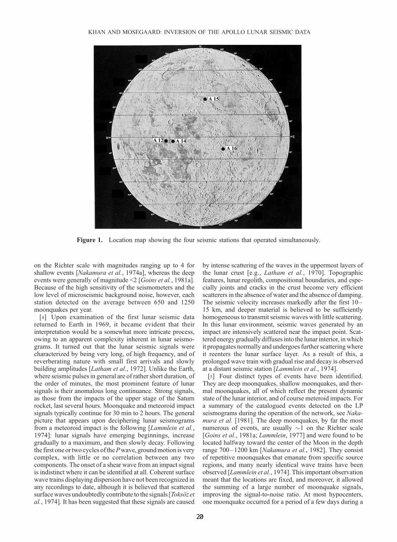
[2] Using seismology to obtain information about theinterior of the Moon saw its advent with the U.S. Apollomissions which were undertaken from July 1969 to Decem-ber 1972. Seismic stations were deployed at five of the sixlocations (Apollo 17 did not carry a seismometer) as part ofthe integrated set of geophysical experiments called theApollo Lunar Surface Experiment Package (ALSEP). Onlyfour of these five stations (12, 14, 15, and 16), powered byradioactive thermal generators, operated concurrently as afour-station seismic array, which was operative from April1972 until 30 September 1977, when transmission of seismicdata was suspended. Each seismic package consisted of threelong-period (LP) seismometers aligned orthogonally tomeasure one vertical (Z ) and two horizontal (X and Y )components of surface motion. The sensor unit also includeda short-period seismometer which was sensitive to verticalmotion at higher frequencies (for more instrumental details,

see Latham et al. [1969]). Digital data were transmittedcontinuously from the lunar surface to receiving stations onEarth and were stored on magnetic tapes for subsequentanalysis. All the seismic data were then displayed on acompressed timescale format from which lunar seismicsignals were identified [Nakamura et al., 1980].[3] The lunar seismic network spans the near face of the

Moon in an approximate equilateral triangle with 1100 kmspacing between stations with two seismometers placed 180km apart at one corner (see Figure 1) and covers mostgeological settings on the front side of the Moon. Since thefirst mission, more than 12,000 events have been recordedand catalogued over a period of 8 years, and it has takenseveral more to evaluate the data [Nakamura et al., 1981].Since the compilation of the recorded seismograms, it hasbeen shown that the Moon is very aseismic compared to theEarth. In comparison to the Earth the energy released inseismic activity is 8 orders of magnitude less, being about1010 J yr�1, compared to 1018 J yr�1 by earthquakes [Goins etal., 1981a], although Nakamura [1980] has pointed out thatthe actual average lunar seismic energy release could be ashigh as 1014 J yr�1. Most of the moonquakes are very small

JOURNAL OF GEOPHYSICAL RESEARCH, VOL. 107, NO. E6, 10.1029/2001JE001658, 2002

Copyright 2002 by the American Geophysical Union.0148-0227/02/2001JE001658$09.00

19

Klaus Mosegaard

Klaus Mosegaard

on the Richter scale with magnitudes ranging up to 4 forshallow events [Nakamura et al., 1974a], whereas the deepevents were generally of magnitude <2 [Goins et al., 1981a].Because of the high sensitivity of the seismometers and thelow level of microseismic background noise, however, eachstation detected on the average between 650 and 1250moonquakes per year.[4] Upon examination of the first lunar seismic data

returned to Earth in 1969, it became evident that theirinterpretation would be a somewhat more intricate process,owing to an apparent complexity inherent in lunar seismo-grams. It turned out that the lunar seismic signals werecharacterized by being very long, of high frequency, and ofreverberating nature with small first arrivals and slowlybuilding amplitudes [Latham et al., 1972]. Unlike the Earth,where seismic pulses in general are of rather short duration, ofthe order of minutes, the most prominent feature of lunarsignals is their anomalous long continuance. Strong signals,as those from the impacts of the upper stage of the Saturnrocket, last several hours. Moonquake and meteoroid impactsignals typically continue for 30 min to 2 hours. The generalpicture that appears upon deciphering lunar seismogramsfrom a meteoroid impact is the following [Lammlein et al.,1974]: lunar signals have emerging beginnings, increasegradually to a maximum, and then slowly decay. Followingthe first one or two cycles of thePwave, groundmotion is verycomplex, with little or no correlation between any twocomponents. The onset of a shear wave from an impact signalis indistinct where it can be identified at all. Coherent surfacewave trains displaying dispersion have not been recognized inany recordings to date, although it is believed that scatteredsurfacewaves undoubtedly contribute to the signals [Toksoz etal., 1974]. It has been suggested that these signals are caused

by intense scattering of the waves in the uppermost layers ofthe lunar crust [e.g., Latham et al., 1970]. Topographicfeatures, lunar regolith, compositional boundaries, and espe-cially joints and cracks in the crust become very efficientscatterers in the absence of water and the absence of damping.The seismic velocity increases markedly after the first 10–15 km, and deeper material is believed to be sufficientlyhomogeneous to transmit seismic waves with little scattering.In this lunar environment, seismic waves generated by animpact are intensively scattered near the impact point. Scat-tered energygradually diffuses into the lunar interior, inwhichit propagates normally and undergoes further scatteringwhereit reenters the lunar surface layer. As a result of this, aprolonged wave train with gradual rise and decay is observedat a distant seismic station [Lammlein et al., 1974].[5] Four distinct types of events have been identified.

They are deep moonquakes, shallow moonquakes, and ther-mal moonquakes, all of which reflect the present dynamicstate of the lunar interior, and of course meteroid impacts. Fora summary of the catalogued events detected on the LPseismograms during the operation of the network, see Naka-mura et al. [1981]. The deep moonquakes, by far the mostnumerous of events, are usually �1 on the Richter scale[Goins et al., 1981a; Lammlein, 1977] and were found to belocated halfway toward the center of the Moon in the depthrange 700–1200 km [Nakamura et al., 1982]. They consistof repetitive moonquakes that emanate from specific sourceregions, and many nearly identical wave trains have beenobserved [Lammlein et al., 1974]. This important observationmeant that the locations are fixed, and moreover, it allowedthe summing of a large number of moonquake signals,improving the signal-to-noise ratio. At most hypocenters,one moonquake occurred for a period of a few days during a

Figure 1. Location map showing the four seismic stations that operated simultaneously.

KHAN AND MOSEGAARD: INVERSION OF THE APOLLO LUNAR SEISMIC DATA

Klaus Mosegaard

20

fixed time in the monthly lunar tidal cycle, giving rise topeaks at 27-day intervals of the observed lunar seismicactivity. In addition, a 206-day variation and a 6-yearvariation in the activity, also due to tidal effects, such as thesolar perturbation of the lunar orbit, have been observed[Lammlein et al., 1974; Lammlein, 1977]. These periodicitieshave been taken as evidence that the deep focus moonquakesare related to the tidal forces acting on the Moon and appearto represent merely a process of storage and release of tidalenergy without a significant release of tectonic energy[Nakamura, 1978; Koyama and Nakamura, 1980].[6] The shallow moonquakes are a manifestation of

another type of natural lunar seismicity. These are the mostenergetic seismic sources observed on the Moon, althoughthey are less abundant than the other types of seismic events,with an average of 4 events per year [Nakamura, 1977]. Theyare also known as high-frequency-teleseismic (HFT) eventsowing to their unusually high frequency content and the greatdistances at which they are observed [Nakamura et al.,1974a]. The estimation of the source depth at which HFTevents occur has been inconclusive, although several lines ofevidence, such as the variation of the observed amplitude ofHFT signals with distance, suggested that they originated nodeeper than a few hundred kilometers [Nakamura et al.,1979]. It has been pointed out that there is no clear correlationbetween them and the tides, as is obvious for deep moon-quakes [Nakamura, 1977]. This led to the conclusion thattheir origin is likely to be tectonic, given their similarity tointraplate earthquakes [Nakamura et al., 1979, 1982]. Theirmechanism, though, could not be explained by plate motion,because of the lack of concentration of events into narrowbelts as is observed on the Earth.[7] A large percentage of the events observed on the short

period components are very small moonquakes, occurringwith great regularity. It is believed that these events, alsotermed thermal moonquakes, are triggered by diurnal ther-mal variations [Duennebier and Sutton, 1974].[8] With the completion of processing of all the lunar

seismic data collected during the Apollo seismic networkoperation, a set of arrival times was obtained, constituting aprimary data set from which the interior velocity structure ofthe Moon could be inferred. The most recent and concisesummary of the seismic velocity profile is based on thecomplete 5-year data set acquired when the four Apolloseismometers were simultaneously operative [Nakamura etal., 1982; Nakamura, 1983]. Nakamura and coworkers haveused arrival times from various seismic events for theelucidation of the seismic velocity profile of the lunar interior.Analysis of the man-made impacts led to a model of theshallow lunar structure, a model for the upper mantle wasconstructed on the basis of the shallow moonquakes and themeteroid impacts, and modeling of the deep lunar interiorwas subject to deep moonquake data. A linearized leastsquares inversion technique using arrival time data from 41deep moonquakes, 7 artificial impacts, 18 meteroid impacts,and 14 shallow moonquakes as compared to only 24 deepmoonquake sources used byGoins et al. [1981b] was appliedin steps. These models established the Moon as a highlydifferentiated body, with a crust and a mantle whose lowerparts were thought to be partially molten [Nakamura et al.,1973]. However, velocity variations and the depths of pos-sible discontinuities in the mantle could not be addressed,

although they were believed to be present [Nakamura, 1983].The central part of the Moon could also not be ascertainedfrom the seismic data owing to the distribution of seismicsources. All confirmed deep moonquakes occurred on thenearside, except for one source, A33, which is located on thefarside beyond the eastern limb. No big meteoroid impactsantipodal to the stations giving rise to unequivocal arrivalswere detected, leaving the important question of the existenceof a lunar core unanswered, although it has to be noted for thesake of completeness that a farside impact, almost diametri-cally opposite to station 15, gave tentative evidence for a low-velocity core with a radius around 400 km [Nakamura et al.,1974b; Sellers, 1992].[9] In the earlier studies mentioned above, the analysis of

the nonlinear inverse problem was primarily centered on theconstruction of best fitting models, thereby obviating theanalysis of uncertainty and nonuniqueness, which are impor-tant items when inferring scientific conclusions from inversecalculations. We [Khan et al., 2000] presented a new P and Swave velocity structure for the Moon from a Monte Carloinversionof theApollo lunar seismic data,whereweadopted aBayesian viewpoint on inverse problems [Tarantola andValette, 1982;Mosegaard and Tarantola, 1995] whose mainfeature is the use of probabilities to describe the modelparameters (which are the ones we invert for) and what lendsitself to their description is the a posteriori probability densityin the model space which summarizes all information aboutthe model we are studying supplied by data, a priori informa-tion, and the physical laws relatingmodel and data. Given thatfor general inverse problems the shape of the posteriorprobability distribution is not known, it cannot simply bedescribed by mathematical means and covariances. TheMarkov ChainMonte Carlo (MCMC) algorithm, on the otherhand, samples a large suite of models from this probabilitydistribution, thereby rendering uswith a better representation.The main purpose of the present study is, on the one hand, todetail themethod of analysis underlying that investigation andmoreover to extend the Bayesian analysis carried out byKhanet al. [2000] (a detailed discussion of the results has alreadybeen given in that study and will not be reiterated here) and asan application of this to investigate the suite of modelssampled via theMCMCalgorithmas to lunar crustal thicknessusing Bayesian hypothesis testing [Bernardo and Smith,1994]. In regard to the data set, no attempt was made toidentify new events or arrivals, and the data used in this studyare the same events as those considered in the study byNakamura [1983], comprising first arrivals of P and Swaves.However, seismograms from these events have been reviewedin order to assess the uncertainty and consistency on thesearrivals. Finally, as regards the outline of the present manu-script, we have chosen first to present general ideas concern-ing (1) the use of MCMC algorithms to solve the generalinverse problem and (2) the analysis of the posterior distribu-tion. Upon this follows a detailed description of the applica-tion of these methods to the Apollo lunar seismic data set.

2. Theory: General Ideas

2.1. Solving the General Inverse Problem Usinga MCMC Algorithm

[10] It is customary to commence an investigation such asthis one by delineating our physical system by a set of


Klaus Mosegaard

21

model parameters, m = (m1, m2,. . ., ms), which completelydefine the system. These parameters are not directly meas-urable. What we usually are in possession of, though, arecertain observable data, d = (d1, d2,. . ., dn), obtainedthrough physical measurements. Now, what we could donext is to try to prognosticate the observable parameters byusing any theory applicable to our particular predicament.This results in another set of parameters, termed calculateddata dcal, which are dependent on the model parameters.This dependency can be depicted by a relation of the form

d ¼ gðmÞ; ð1Þ

g being a functional relation governing the physical laws thatcorrelate model and data. What is meant by solving theforward problem, then, is the prediction of observable datagiven a set of model parameters, and conversely, solving theinverse problem is understood to be the inference of values ofthe model parameters, given observable data. Central to ourmethod is the notion of a state of information over theparameter set. In concordance with the most generaldescription of states of information over a given parameterset, as presented by Tarantola and Valette [1982] andTarantola [1987], we shall be employing probabilitydensities over the corresponding parameter space, describingthe various states of information inherent to our system. Thisknowledge embodies the results of measurements of theobservable parameters and the a priori information on modelparameters as well as the information on the physicalcorrelations between observable and model parameters.Solving the inverse problem, then, shall be formulated as aproblem of combining all this information into an alteriorstate, termed the posterior probability density. The extensiveuse of probability densities for delineating any informationhas the advantage of presenting the solution to the inverseproblem in the most generic way, thereby implicitlyincorporating any nonlinearities [Tarantola and Valette,1982].[11] It is clear, then, that the most general method for

solving nonlinear inverse problems needs an extensiveexploration of the model space, since the posterior proba-bility density in the model space contains all the informationabout the system being studied. Therefore, given probabil-istic prior information on m and a statistical description ofthe observational uncertainties of d, the main idea is todesign a random walk in the model space which samples theposterior probability distribution, that is, samples modelswhich are consistent with data as well as prior information.To this end, we shall use a Markov Chain Monte Carloalgorithm of the following form (the basic premises under-lying the use of MC algorithms to solve general inverseproblems are reviewed by Mosegaard [1998]):1. Propose a new model, mpert, by taking a step of a

random walk to some current model mcur, with a probabilityproportional to r(m), the prior probability density on themodel parameters.2. Calculate the likelihood function for the new model

using L(m) = k�exp(�S(m), where k is a normalizationconstant, S(m) is the misfit function, and L(m) is a measureof the degree of data fit.3. Accept the new model with a probability Pacc ¼

minð1; LðmpertÞ=LðmcurÞÞ:

4. If mpert is accepted, then mcur = mpert. If not, thenreapply mcur and repeat the above steps.[12] This algorithm will sample the posterior probability

density

sðmÞ ¼ hrðmÞLðmÞ; ð2Þ

h being a normalization constant, asymptotically. ‘‘Asymp-totically,’’ in this case, implies that the statistical correlationbetween samples taken at times separated by n iterationswill converge toward zero as n goes to infinity. Theadvantage of using the above scheme to sample theposterior probability density s(m) is that sampling isconferred to those parts of the model space where modelparameters consistent with data and prior information exist.

2.2. Analysis of the Posterior Distribution

[13] Having designated the posterior probability distribu-tion s(m) as the solution to our inverse problem, our mainconcern is now the analysis of this distribution. However,owing to its complex shape (it might be multimodal, containinfinite variances, etc.), it is not possible to directly accessinformation from it. Instead, the information of most use isobtained by investigating the probability P that a certainfeature resides at a given depth or depth range (correspond-ing to the model parameters being contained within a givensubset of the model space), which can be calculated from

Pðm 2 �Þ ¼R� sðmÞdmR� sðmÞdm ; ð3Þ

where � denotes a subset of the model space � and thedenominator is clearly identified as a normalization factor.This can easily be extended to the calculation of means andcovariances.[14] We could also adopt the point of view taken by

Mosegaard [1998], who states that the main aim ofresolution analysis is to aid in having to choose betweendiffering interpretations of a given data set. In line here-with our principal purpose in analyzing the sampledmodels will basically be to conjure up queries addressingcorrelations between several model parameters. The onequestion that we intend to investigate using the sampledmodels concerns the lunar crust and could be formulatedas follows:. How likely is it, on the basis of the seismic data and

their uncertainties as well as prior information, that theMoon has a discontinuity (suitably defined) in a certaindepth range, marking for example the crust-mantle inter-face?However, answering questions like these involves having toevaluate resolution measures of the form [Mosegaard,1998]

Rð�; f Þ ¼Z�

f ðmÞsðmÞdm; ð4Þ

where f (m) is a given function of the model parameters mand � is, as in (3), an event or subset of the model space �containing the models of current interest. The similaritybetween (3) and (4) is obvious.


Klaus Mosegaard

22

[15] It is clear from the above discussion that in the caseof the general inverse problem, (3) and (4) are inaccessibleto analytical evaluation, since we do not have an analyticalexpression for s(m). However, the problem can be solvedusing the MCMC algorithm, as mentioned before, whichsamples a large collection of models, m1, m2, . . . , mn, froms(m), whereby the resolution measure, given by (4), in turncan be approximated by the following simple average[Mosegaard, 1998]:

Rð�; f Þ 1

N

Xfnjmn2�g

f ðmnÞ; ð5Þ

where N normalizes the resolution measure. For the numberof samples N ! 1 the equality of (4) and (5) correspondsto the important ergodicity property used in Monte Carlointegration.[16] However, we shall avail ourselves of a slightly

different approach which is known as hypothesis testing.While the two analyses basically amount to the same, sincea hypothesis corresponds to a question, the advantage inhypothesis testing lies in the fact that we are able tocompare any two hypotheses against each other.[17] The classical problem of hypothesis testing concerns

itself with making a choice among different hypotheses,H1,H2,. . . , Hn, on the basis of some observed data d. Orformulated alternatively, we might be in the position ofhaving to decide how the prior probability P(H), concern-ing any hypothesis H, has been amended by taking intoaccount observed data d (henceforth abbreviated data); thatis, we are interested in evaluating P(H|d), which is usuallytermed the posterior probability distribution. The mathe-matical connection linking the prior and the posterior isgiven by the Bayes theorem

PðHjdÞ ¼ hPðdjHÞPðHÞ; ð6Þ

where h is a normalization constant. Extending the analysisin order to compare any two hypotheses, we arrive at theBayes factor, whose definition has been ascribed to Turing[e.g., Good, 1988].2.2.1. Definition (Bayes factor)

[18] Given two hypotheses Hi, Hj corresponding todifferent areas of the model space �, for data d, the Bayesfactor Bij in favor of Hi (and against Hj) is given by theposterior to prior odds ratio.

BijðdÞ ¼PðdjHiÞPðdjHjÞ

¼PðHijdÞ=PðHj

��dÞPðHiÞ=PðHjÞ

; ð7Þ

P(d|Hi) being the probability distribution, usually termedthe likelihood (see below). Thus the Bayes factor provides ameasure of whether the data d have increased or decreasedthe odds on Hi relative to Hj. Accordingly, if Bij(d) > 1, Hi

is now more relatively plausible than Hj in the light of d; onthe other hand, if Bij(d) < 1, it signifies that Hj has nowincreased in relative plausibility [Bernardo and Smith,1994]. It is clear that apart from how one defines the crust-mantle transition or any other hypothesis for that matter, thisform of analysis is straightforward as seen from the

Bayesian viewpoint. This can be appreciated by rewritingthe above equation as

PðHijdÞPðHj

��dÞ ¼ PðdjHiÞPðdjHjÞ

� PðHiÞPðHjÞ

; ð8Þ

that is, the ratio of posterior odds equals the integratedlikelihood ratio times the ratio of prior odds. Thisequation shows explicitly how the ratio of integratedlikelihoods plays the key part in providing the mechanismby which data transform relative prior beliefs into relativeposterior beliefs. If we compare this to the form of theposterior probability distribution, equation (2), which weused in sampling solutions to our inverse problem, theconnection is complete, in that (2) states in an analogousmanner the role of the likelihood function L(m), whichcontains information on data d and on the physicaltheories linking data and model parameters, in changingthe prior probability distribution on model parametersr(m) into the posterior s(m) [Mosegaard and Tarantola,1995; Mosegaard, 1998].

3. Analysis: Application of the MCMC Algorithmto the Apollo Lunar Seismic Data

3.1. Forward Problem

[19] As mentioned, the forward problem consists of calcu-lating data, that is, travel times, given a set of modelparameters, that is, a model of the subsurface velocitystructure, among other things. In our model of the Moon theassumption of radial symmetry is made. The Moon is parti-tioned into 56 shells of variable size, with each layer beingcharacterized by its physical extent andmaterial parameters inthe form of the velocity. To each shell is assigned a piecewiselinearly varyingP and Swave velocity of the form v(r) = vo+ k� r, which is continuous at layer boundaries. In order toaccommodate ray theory, certain limits are placed on thevelocity gradients, resulting in a smoothness constraint limit-ing vertical resolution to roughly 5 km.[20] Since the Moon is neither spherically symmetric nor

geologically homogeneous, an additional asset was intro-duced to facilitate a more realistic modeling of the lunarinterior. Our model of the Moon was stripped of a surficiallayer, 1 km thick, which is known to be of very low velocity[Kovach and Watkins, 1973]. Because of the extremevelocity gradients encountered by the rays when impingingthis layer, they will be almost vertically incident uponreaching the surface. The travel time for a ray in this layerwill therefore to a good approximation be given by T =1 km/vsurface. So, instead of ray tracing in a sphere with aradius of 1738 km, we traced in one with a radius of1737 km and added for every station and surface source atime correction to the travel time. Starting off with a surfacevelocity of, say, 0.5 km s�1 [Nakamura et al., 1982] meansthat we have to add a total time correction of 4 s to the traveltime of a ray emanating from a surface source and 2 s forone originating within the Moon. Leaving the time correc-tions variable, this method has the added advantage oftaking localized properties of the surficial material beneatheach station into account. For consistency, all time correc-tions have been correlated in such a way that if a particularstation has been assigned a given initial correction, this


Klaus Mosegaard

23

same correction will be added to the travel times for the raysemitted from all sources and traveling to this particularreceiver. In the same way, the corrections are correlated forthe impacts; that is, all rays emanating from a particularimpact have the same correction added to their total traveltime.

3.2. Inverse Problem

[21] Three parameters as discussed in the previous sec-tion are used to describe our physical model of the Moonwhich included the position of the layer boundaries, ri, theirvelocities, vi, and the time corrections, tk, in the surficiallayer. In choosing how to parameterize our physical system,however, it has to be noted that the choice of whichparameterization to employ is an ambiguous matter, in thesense that it is not unique [Tarantola and Valette, 1982]. So,instead of examining a number of different parameteriza-tions, such as the velocity or the slowness, we shall availourselves of another approach, this being the invarianceargument. As the name suggests, invariance implies theprocurement of commensurate distributions upon transfor-mation from any one invariant measure. The ‘‘log-velocity’’possesses exactly this property [Tarantola, 1987]; that is,given a uniform distribution in log(v/vo), for example, wewill achieve a similar distribution whether it be the velocityor the slowness we are transforming to. We shall thereforeadopt log(v/vo) as the parameterization throughout thisstudy. (In the following we shall continue to use vi todescribe the velocity parameters, but it is tacitly assumedthat we actually mean the log-velocity. Throughout thisstudy, vo = 1.0 km s�1.)[22] To fully characterize our physical system, we also

need to incorporate parameters which describe the meteor-oid impact as well as the shallow and deep moonquakelocations, thus resulting in the addition of three otherparameters in the delineation of our model. These parame-ters are the depth coordinate of every moonquake and theselenographical position of the epicenter, that is, longitudeand latitude, which we shall label sj and the latter two qj andfj, respectively. Our model is thus ultimately given by m ={ri, vi, tk, sj, qj, fj}.[23] In commencing the MCMC algorithm we started

out by assuming some initial model m, henceforth mcur,comprising a set of values. Now, by perturbing one ofthese parameters, that is, by either changing the positionof a boundary layer, changing the value of the velocity ata given layer boundary, assigning a new time correctionfor either a source or a station, or amending the hypo-central or epicentral coordinates depending on the partic-ular event, we obtain a new model. The random walker isthen set out to sample the parameter space according tothe prior information and using a set of random ruleswhose efficiency has been optimized through severalnumerical experiments. Let us outline these random rulesand the prior information. For every iteration it is firstdecided which parameter is to be perturbed next. Thedecision is made whether to change a parameter pertain-ing to the lunar interior or one regarding the location of aseismic event, which are equally probable. Performing avelocity perturbation has the same probability (0.5) asperforming a boundary layer perturbation. When it comesto perturbing the time corrections, these are set to be

amended every fifth iteration. When perturbing either thevelocity or the position of a boundary, the layer isselected uniformly at random and so is the value of theparameter to be changed. It should be kept in mind thatperturbations concerning the placement of boundarieshave in a certain sense been restricted in order toaccommodate ray theory. Every layer to be perturbedcan be assigned any value, except in a range of 5 kmwithin the layer immediately above or below; that is, anygiven layer i can assume a value within ri � 1 + 5 km �ri � ri + 1 � 5 km. Concerning the time amendments,whether it is a source location or the location of a station,which is to be perturbed will be chosen uniformly atrandom, as are their values. Let us note that we havemade the assumption of a uniform distribution in the ‘‘log-time’’ domain as in the case of the velocities, the reasonbeing that the time is directly related to the velocities inthe top layer. Concerning the hypocenter coordinates, thesource depths are uniformly distributed from the surfaceto the center of the Moon, and the epicentral coordinatesare likewise assumed to be uniformly distributed, in thiscase across the lunar surface. As regards the sampling ofS wave velocities, it has to be remarked that in order tomake the inversion tractable the problem was actuallydivided into two stages. The first entailed the inversion ofthe P wave arrival times, while the second considered theinversion of the S wave arrivals. Now, it is clear that thetwo parameters, vp and vs, are not independent ifdescribed in terms of the elastic moduli, r, k, and m,these being the density, bulk, and shear modulus, respec-tively. It could therefore be argued that this division ofthe problem might result in physically unrealizable mod-els (for further discussion, see section 8). However, beingaware of the connection between the two parameters, wedid impose certain constraints on the sampling of S wavevelocities, corresponding to the addition of prior informa-tion, by introducing a Gaussian distribution centered onthe average vp

� ffiffiffi3

pas obtained from the first inversion

and with a standard deviation given by svp� ffiffiffi

3p

. Thisprior information thus signifies that S wave velocitieslying far from this distribution are less likely sampled.[24] This body of information, then, serves as prior

knowledge, in the sense that the random walker will besampling the model space with a probability densitydescribing exactly this information.[25] At this point the reader might wonder about what

happened to the estimation of parameters pertaining to theorigin time of events, since these are also unknowns when itcomes to event localization. These are also determined inthis study; however, instead of including these in the modelparameter vector m above as another set of parameters to bedetermined, we adopted a slightly different approach.[26] Generally, we have the following relation concerning

the arrival times:

da ¼ mo þ gðmÞ;

where da is the vector of arrival times, mo is a modelparameter vector of origin times corresponding to individualarrivals, and g(m) is our set of calculated travel times. Now,for the present purposes we made the assumption that the a


Klaus Mosegaard

24

priori information concerning the origin time modelparameters was normally distributed with mean values asdetermined by the Nakamura model [Nakamura et al.,1976; Nakamura, 1983] and an a priori uncertainty,typically of a few seconds. This sets the stage for thefollowing formal definition of new data:

d ¼ da �mo:

To these were assigned a new standard deviation as the sumof the standard deviation of arrival times and the a prioridispersion on origin time model parameters, thus defining acomposite uncertainty (to be dealt with later on).[27] The reason that we ended up choosing what might be

labeled rather loose prior knowledge on model parameters,by assuming that they were all uniformly distributed withina large range, was our main aim of wanting to investigatethe full model variability inherent in the lunar seismic data.[28] Having designated prior information, let us continue

the MCMC algorithm and assume that the random walkerwishes to sample the velocity at some depth. He currentlyresides at vi and from there takes a step in some direction toa point vi

new. Now, we do not restrict the random walker towander within some specified range, but shall rather let himdrift around the model space from zero to infinity, althoughevery jump is in a sense constrained so as to assure that therandom walker can take only small steps. Sampling the apriori distribution by this method basically corresponds tothe process of diffusion, since the random walker canessentially, if given steps enough, explore the whole modelspace. Mathematically, we would write this condition asvinew = vi + x � (2 � a � 1), where a denotes a uniformly

distributed number in the interval [0,1] and x is a constant,typically of the order of 0.2 km s�1 in this study.[29] After having obtained a new model, mpert, our next

step is to gauge the posterior distribution. This we do byfirst calculating a new set of arrival times using g(mpert) andthen comparing these to the observed data in order to obtainthe misfit function. This misfit is of importance, since weshall by the Metropolis rule use it to either accept or rejectthe new model, with probability Pacc = min{1, L(mpert)/L(mcur)}. In words, we could state this by saying that therandom walker essentially updates his knowledge of thecurrent state of affairs, as prescribed by Bayes’ theorem, bymerging together prior information with data and theory.The revision of the prior into the posterior is illustrated in

Figure 2, which shows how a prior distribution for a givenvelocity parameter is being changed as data are taken intoaccount. Moreover, we are led to the conclusion that thelevel of confinement is a direct measure of the knowledgewe possess about the system; that is, the more the randomwalker is constrained when sampling the posterior distribu-tion in the model space, the greater is our degree ofknowledge.[30] Now, the strategy set forth here of perturbing only

one parameter at a time is sure to preserve most of thecharacteristics of the current model which may haveresulted in a good data fit. While being efficient, in thesense that we are interested in sampling models with a gooddata fit, this strategy will result in a sequence of samples,that is, models, that tend to be correlated. This is somewhatunfortunate, since analyses of error and resolution require acollection of statistically independent models from theposterior distribution. The way to proceed is to choosefewer samples from the set of accepted models in such away that they constitute a set of independent models. Thiscan be done by introducing an elapse time (number ofiterations) between retention of samples which was foundby analyzing the fluctuations of the likelihood function asthe algorithm proceeded to be 100. Inspection of theautocorrelation function for these fluctuations showed thataccepted models separated by 100 iterations were unlikelyto be correlated. On the other hand, the limited number ofiterations performed may not be sufficient to allow thealgorithm to visit enough extrema in the model space. Tocircumvent this problem, we chose to commence at differentplaces in the model space for every 10,000 iterationsperformed by the algorithm. This was done by restartingthe MCMC algorithm with different initial values at thoseintervals. This procedure should guarantee that the samplesare less correlated as well as leading to a better coverage ofthe probability distribution. (It should be noted thatalthough this method is more efficient in detecting mostof the extrema, its downside is the fact that it is biasedtoward an approximately equal coverage of them all. Theglobal extremum, corresponding to the most likely solution,might end up being sampled on a par with secondaryextrema, thereby conferring them with equal weight.) Toensure that the posterior probability density was adequatelysampled in our analysis, we monitored the time series of alloutput parameters from the algorithm to verify that thesewere indeed stationary over the many iterations performed.

Figure 2. Prior and posterior marginal log(v/vo) parameter distribution. Note how the prior is changedfrom sampling a uniform distribution by taking data into account so as to sample the posterior.


Klaus Mosegaard

25

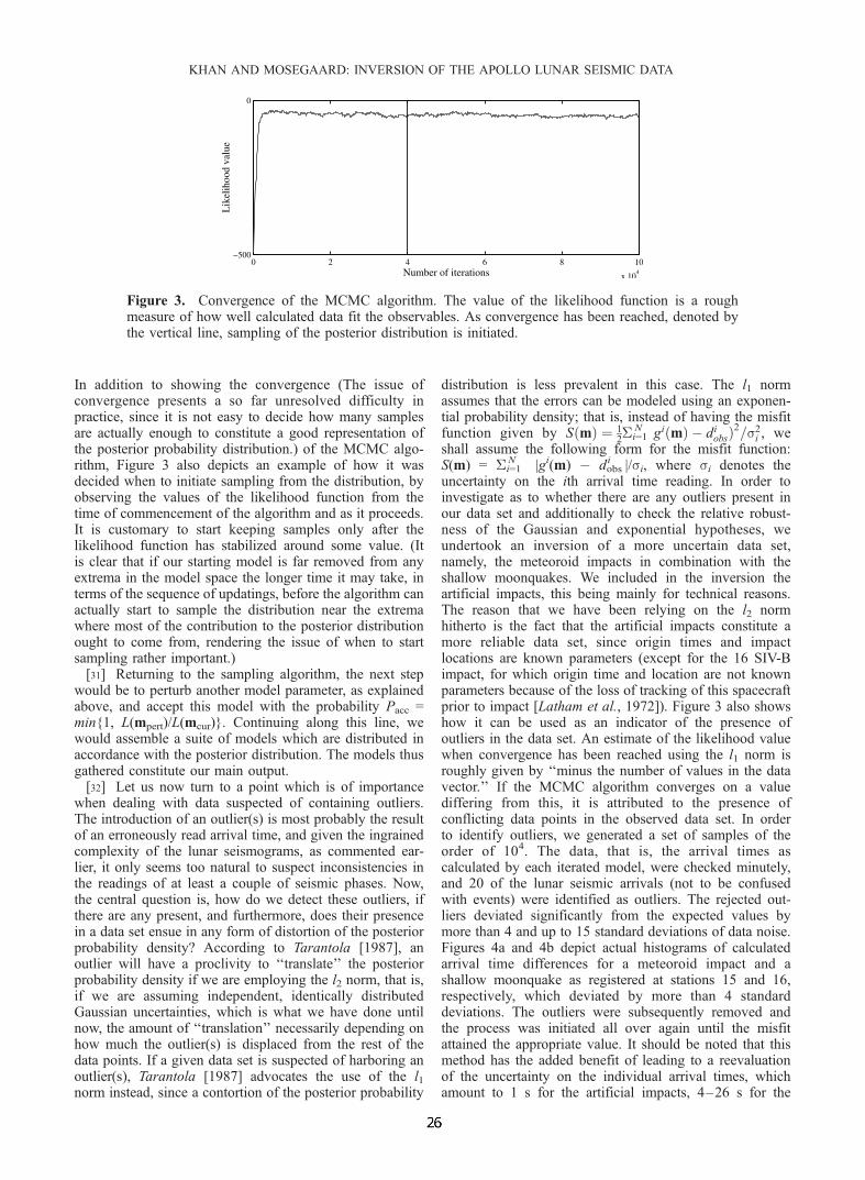
In addition to showing the convergence (The issue ofconvergence presents a so far unresolved difficulty inpractice, since it is not easy to decide how many samplesare actually enough to constitute a good representation ofthe posterior probability distribution.) of the MCMC algo-rithm, Figure 3 also depicts an example of how it wasdecided when to initiate sampling from the distribution, byobserving the values of the likelihood function from thetime of commencement of the algorithm and as it proceeds.It is customary to start keeping samples only after thelikelihood function has stabilized around some value. (Itis clear that if our starting model is far removed from anyextrema in the model space the longer time it may take, interms of the sequence of updatings, before the algorithm canactually start to sample the distribution near the extremawhere most of the contribution to the posterior distributionought to come from, rendering the issue of when to startsampling rather important.)[31] Returning to the sampling algorithm, the next step

would be to perturb another model parameter, as explainedabove, and accept this model with the probability Pacc =min{1, L(mpert)/L(mcur)}. Continuing along this line, wewould assemble a suite of models which are distributed inaccordance with the posterior distribution. The models thusgathered constitute our main output.[32] Let us now turn to a point which is of importance

when dealing with data suspected of containing outliers.The introduction of an outlier(s) is most probably the resultof an erroneously read arrival time, and given the ingrainedcomplexity of the lunar seismograms, as commented ear-lier, it only seems too natural to suspect inconsistencies inthe readings of at least a couple of seismic phases. Now,the central question is, how do we detect these outliers, ifthere are any present, and furthermore, does their presencein a data set ensue in any form of distortion of the posteriorprobability density? According to Tarantola [1987], anoutlier will have a proclivity to ‘‘translate’’ the posteriorprobability density if we are employing the l2 norm, that is,if we are assuming independent, identically distributedGaussian uncertainties, which is what we have done untilnow, the amount of ‘‘translation’’ necessarily depending onhow much the outlier(s) is displaced from the rest of thedata points. If a given data set is suspected of harboring anoutlier(s), Tarantola [1987] advocates the use of the l1norm instead, since a contortion of the posterior probability

distribution is less prevalent in this case. The l1 normassumes that the errors can be modeled using an exponen-tial probability density; that is, instead of having the misfitfunction given by S mð Þ ¼ 1

2�i=1

N gi mð Þ � diobsÞ2=s2i , we

shall assume the following form for the misfit function:S(m) = �i=1

N |gi(m) � dobsi |/si, where si denotes the

uncertainty on the ith arrival time reading. In order toinvestigate as to whether there are any outliers present inour data set and additionally to check the relative robust-ness of the Gaussian and exponential hypotheses, weundertook an inversion of a more uncertain data set,namely, the meteoroid impacts in combination with theshallow moonquakes. We included in the inversion theartificial impacts, this being mainly for technical reasons.The reason that we have been relying on the l2 normhitherto is the fact that the artificial impacts constitute amore reliable data set, since origin times and impactlocations are known parameters (except for the 16 SIV-Bimpact, for which origin time and location are not knownparameters because of the loss of tracking of this spacecraftprior to impact [Latham et al., 1972]). Figure 3 also showshow it can be used as an indicator of the presence ofoutliers in the data set. An estimate of the likelihood valuewhen convergence has been reached using the l1 norm isroughly given by ‘‘minus the number of values in the datavector.’’ If the MCMC algorithm converges on a valuediffering from this, it is attributed to the presence ofconflicting data points in the observed data set. In orderto identify outliers, we generated a set of samples of theorder of 104. The data, that is, the arrival times ascalculated by each iterated model, were checked minutely,and 20 of the lunar seismic arrivals (not to be confusedwith events) were identified as outliers. The rejected out-liers deviated significantly from the expected values bymore than 4 and up to 15 standard deviations of data noise.Figures 4a and 4b depict actual histograms of calculatedarrival time differences for a meteoroid impact and ashallow moonquake as registered at stations 15 and 16,respectively, which deviated by more than 4 standarddeviations. The outliers were subsequently removed andthe process was initiated all over again until the misfitattained the appropriate value. It should be noted that thismethod has the added benefit of leading to a reevaluationof the uncertainty on the individual arrival times, whichamount to 1 s for the artificial impacts, 4–26 s for the

Figure 3. Convergence of the MCMC algorithm. The value of the likelihood function is a roughmeasure of how well calculated data fit the observables. As convergence has been reached, denoted bythe vertical line, sampling of the posterior distribution is initiated.


Klaus Mosegaard

26

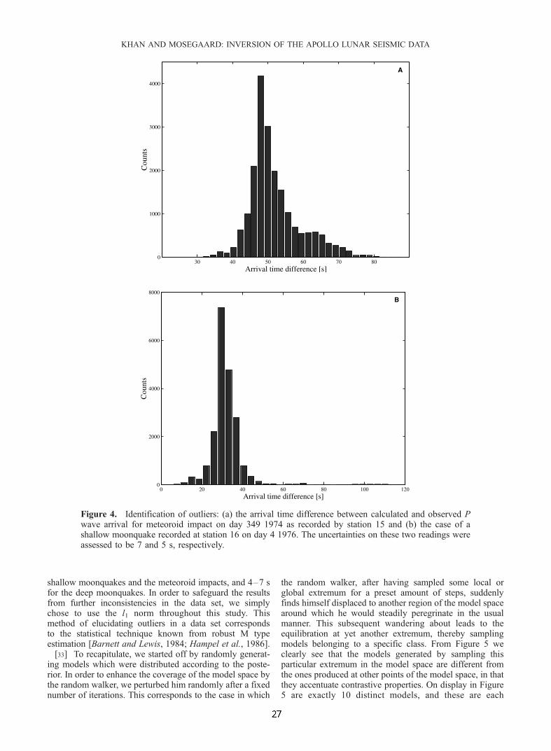
shallow moonquakes and the meteoroid impacts, and 4–7 sfor the deep moonquakes. In order to safeguard the resultsfrom further inconsistencies in the data set, we simplychose to use the l1 norm throughout this study. Thismethod of elucidating outliers in a data set correspondsto the statistical technique known from robust M typeestimation [Barnett and Lewis, 1984; Hampel et al., 1986].[33] To recapitulate, we started off by randomly generat-

ing models which were distributed according to the poste-rior. In order to enhance the coverage of the model space bythe random walker, we perturbed him randomly after a fixednumber of iterations. This corresponds to the case in which

the random walker, after having sampled some local orglobal extremum for a preset amount of steps, suddenlyfinds himself displaced to another region of the model spacearound which he would steadily peregrinate in the usualmanner. This subsequent wandering about leads to theequilibration at yet another extremum, thereby samplingmodels belonging to a specific class. From Figure 5 weclearly see that the models generated by sampling thisparticular extremum in the model space are different fromthe ones produced at other points of the model space, in thatthey accentuate contrastive properties. On display in Figure5 are exactly 10 distinct models, and these are each

Figure 4. Identification of outliers: (a) the arrival time difference between calculated and observed Pwave arrival for meteoroid impact on day 349 1974 as recorded by station 15 and (b) the case of ashallow moonquake recorded at station 16 on day 4 1976. The uncertainties on these two readings wereassessed to be 7 and 5 s, respectively.


Klaus Mosegaard

27

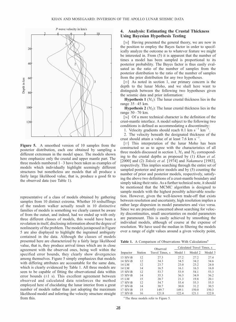
representative of a class of models obtained by gatheringsamples from 10 distinct extrema. Whether 10 reshufflingsof the random walker actually result in 10 distinctivefamilies of models is something we clearly cannot be awareof from the outset, and indeed, had we ended up with onlythree different classes of models, this would have been arevelation in itself, disclosing information about the degree ofnonlinearity of the problem. The models juxtaposed in Figure5 are also displayed to highlight the ingrained ambiguitycontained in the data. Although the classes of modelspresented here are characterized by a fairly large likelihoodvalue, that is, they produce arrival times which are in closeagreement with the observed ones, being well within thespecified error bounds, they clearly show divergenciesamong themselves. Figure 5 simply emphasizes that modelswith differing attributes are accountable for the same data,which is clearly evidenced by Table 1. All three models areseen to be capable of fitting the observational data withinerror bounds (±1 s). This excellent agreement betweenobserved and calculated data reinforces the methodemployed here of elucidating the lunar interior from a greatnumber of models rather than just adopting the maximumlikelihood model and inferring the velocity structure straightfrom this.

4. Analysis: Estimating the Crustal ThicknessUsing Bayesian Hypothesis Testing

[34] Having presented the general theory, we are now inthe position to employ the Bayes factor in order to specif-ically analyze the outcome as to whatever feature we mightbe interested in. From (5) it is apparent that the number oftimes a model has been sampled is proportional to itsposterior probability. The Bayes factor is thus easily eval-uated as the ratio of the number of samples from theposterior distribution to the ratio of the number of samplesfrom the prior distribution for any two hypotheses.[35] As noted in section 1, our primary concern is the

depth to the lunar Moho, and we shall here want todistinguish between the following two hypotheses giventhe seismic data and prior information:Hypothesis 1 (H1): The lunar crustal thickness lies in the

range 35–45 km.Hypothesis 2 (H2): The lunar crustal thickness lies in the

range 50–70 km.[36] Of a more technical character is the definition of the

crust-mantle interface. A model subject to the following twoconditions is defined as accommodating a discontinuity:1. Velocity gradients should reach 0.1 km s�1 km�1.2. The velocity beneath the designated thickness of the

crust should attain a value of at least 7.6 km s�1.[37] This interpretation of the lunar Moho has been

constructed so as to agree with the characteristics of allthree models discussed in section 1, H1 and H2 correspond-ing to the crustal depths as proposed by (1) Khan et al.[2000] and (2) Toksoz et al. [1974] and Nakamura [1983],respectively. This implies searching through the entire set ofsampled posterior and prior models and by (5) counting thenumber of prior and posterior models, respectively, satisfy-ing the above two definitions of a crust-mantle boundary andsimply taking their ratio. As a further technical note, it shouldbe mentioned that the MCMC algorithm is designed tosample models with the highest possibly achievable resolu-tion. However, given the well-known trade-off that existsbetween resolution and uncertainty, high resolution implies arather large dispersion in model parameters and vice versa.Since we are presently concerned about searching for veloc-ity discontinuities, small uncertainties on model parametersare paramount. This is easily achieved by smoothing theindividual models, although of course at the expense ofresolution. We have used the median in filtering the modelsover a range of eight values around a given velocity point,

Figure 5. A smoothed version of 10 samples from theposterior distribution, each one obtained by sampling adifferent extremum in the model space. The models shownhere emphasize only the crustal and upper mantle part. Thethree models numbered 1–3 have been taken as examples ofmodels which individually highlight seemingly differentstructures but nonetheless are models that all produce afairly large likelihood value, that is, produce a good fit tothe observed data (see Table 1).

Table 1. A Comparison of Observations With Calculationsa

Impactor StationObserved

Travel Times, s

Calculated Travel Times, s

Model 1 Model 2 Model 3

13 SIV-B 12 27.3 27.2 27.2 27.414 SIV-B 12 34.3 34.5 34.2 34.614 LM 12 23.7 23.0 23.2 24.014 LM 14 16.5 16.1 16.3 16.015 SIV-B 12 53.7 53.9 54.1 53.315 SIV-B 14 35.3 36.3 34.9 36.215 LM 15 20.7 21.3 19.8 20.117 SIV-B 12 54.7 55.4 55.3 55.517 SIV-B 14 30.7 30.0 31.2 30.517 SIV-B 15 149.7 149.1 150.0 150.317 SIV-B 16 121.8 122.4 121.1 122.0

aThe three models refer to Figure 5.


Klaus Mosegaard

28

since the median preserves any discontinuities rather thansmoothing them.[38] The posterior and prior odds ratios were found to be

P(H1|d)/P(H2|d) = 2.5 and P(H1)/P(H2) = 0.6, respec-tively, resulting in a Bayes factor of

B12 ¼PðH1jdÞ=PðH2jdÞPðH1Þ=PðH2Þ

¼ 2:5

0:6¼ 4:2;

whereby H1 is favored to H2 given data and priorinformation.

5. Interpretation of the Results

[39] As emphasized previously, the solution to the Baye-sian formulation of general inverse problems results in a

posterior probability distribution and not single estimates,although these can be obtained from the posterior distributionby numerical integration. What this signifies is that we aresolely working with solutions in terms of probability distri-butions, and moreover, given the multidimensional nature ofthe posterior distribution, it is not accessible for direct displayand only marginals can be exhibited. Therefore care must beexercised in interpreting the outcome, since false conclusionsand overinterpretations are easily reached.[40] Now, from Figure 6, depicting the final velocity

model, it would seem very natural to assume the modelbelonging to the region of highest probability as theprevalent one and therefore pick it as the main lunarvelocity structure. However, this particular model willusually not correspond to the most likely model (which istypical of strongly nonlinear problems and is clarifiedfurther below), since it has to be remembered that the

Figure 6. The marginal posterior velocity distributions depicting the velocity structure of the Moon. Atotal of 50,000 models have been used in constructing the two results. For each kilometer a histogramreflecting the marginal probability distribution of sampled velocities has been set up. By lining up thesemarginals, the velocity as a function of depth is envisioned as contours directly relating their probabilityof occurrence. The contour lines define nine equal-sized probability density intervals for the distributions.The uncertainties on the results are in part due to the large uncertainty in arrival time readings. It shouldbe kept in mind that the velocity models are depicted using marginal probability distributions, and as sucha model incorporating velocities of maximum probability does not necessarily correspond to the mostlikely model. See color version of this figure at back of this issue.


Klaus Mosegaard

29

velocity models shown here have been displayed usingmarginal posterior probability distributions, one-dimen-sional (1-D) marginals, actually. What this means is that ifwe were to choose the most probable velocity at a givendepth, this would correspond to the most likely velocity atthis particular depth only, while disregarding the informa-tion on all other parameters.[41] Given that s(m) is a rather complicated entity, it is

more convenient and probably also sufficient for generalorientation regarding the uncertainty about m simply todescribe regions of given probability under s(m). From thispoint of view the identification of intervals containing 50, 90,or 99% of the probability under s(m) might actually suffice togive a good idea of the general quantitative messages implicitins(m), leading us to the calculation of credible intervals. Thecredible interval is defined as the shortest possible intervalcontaining a given probability, and in Figure 7 we havedepicted credible intervals containing 99% of the marginalprobability.At first glance these credible intervals appear to bequite broad,which essentially indicates that the absolute valueof the velocity in a given layer is not very well determined. Asa consequence, the interpretation of the marginals shown inFigure 6 is a subtle issue where the use of qualities such asprudence and restraint are to be advocated. For example, if ithappens that at a certain depth or within a certain depth rangethere might be a large probability for a somewhat high

velocity, this is, because of the aforementioned ill-determinednature of the absolute velocities, by nomeans to be interpretedas the results stating this particular fact.[42] This conundrum inherent in nonlinear problems is

further illustrated with the following simple example. Fig-ure 8a shows the nonlinear function investigated for thepurpose (a third-degree polynomial). Also included is thetrue model, mtrue, giving rise to noise-free data dtrue. Let usimagine that we have performed some sort of physicalmeasurement which results in an observed datum, dobs,which is also shown. Let us also assume, mainly for sim-plicity, that noise concerning this data point is normallydistributed with uncertainty s. In this particular example,dobs turns out to be displaced one s from dtrue (experimentaldetails are included in the caption of Figure 8). Now, thesituation is this: we have measured a datum, dobs, and giventhis observation we would like to infer information about themodel m (here one model parameter) by computing itsposterior probability density (the prior probability densityis assumed constant). What has been said so far is exactlywhat we have been describing hitherto in dealing with inverseproblems. Next, the posterior probability distribution for a setof model parameter values is easily calculated, and Figure 8bshows this probability distribution. Here mtrue has also beendepicted, and it is obvious that the true model is situated farfrom the model of maximum posterior probability.[43] This example more than anything else reveals the

intricacies hidden in nonlinear problems and explains whythe most probable model is not necessarily the one ofutmost interest, since it might be far displaced, as indeedit is in the example outlined here (by more than 100%),from the true model, and this in spite of the fact that data

Figure 7. The lunar P wave velocity structure shownusing 99% credible intervals. The broad velocity rangesevince the uncertainties involved. The structure in themiddle shows the Nakamura velocity model [Nakamura etal., 1982] so as to highlight consistency with earlier models.

Figure 8. A simple illustration of a nonlinear problem: (a)the nonlinear function and (b) the posterior probabilitydistribution for the model parameterm. Here the true model isdisplaced bymore than 100% from themodelwith the greatestposterior probability, ultimately showing that care has to beexercised in interpreting the outcome of nonlinear problems.Details of the experiment are as follows: g(m) = (am)3 + bm,where a = 0.7 and b = 700; dobs is assumed to be Gaussiandistributed with uncertainty s = 105 and whose actual value isgiven by dtrue + s. The posterior probability distribution iscalculated from L(m) = exp(�||dobs � g(m)||2/2s2).


Klaus Mosegaard

30

uncertainty has been modeled using a Gaussian distribution.With this example in mind it is also clear why, in the case ofnonlinear problems, the model with the highest posteriorprobability does not necessarily correspond to the rightsolution and thus why interpretations using the most prob-able model can be erroneous.[44] Returning to the credible intervals, we further

superposed the Nakamura model on top of our credibleintervals to highlight consistency. Although the Nakamuramodel at certain ranges lies just barely within ours, it isnonetheless contained within the 99% credible region,which shows that there is no inconsistency between ourresults and his model.[45] On the other hand, an item which turns out to be

well determined is the existence of a velocity discontinu-ity. This is easily evidenced using two-dimensional mar-ginals. As an example, we plotted in Figure 9 the marginalprobability distribution among two model parameters, theP wave velocity at 500 km and at 580 km depth,respectively, which depicts the correlation that existsbetween the two model parameters. From this it is appa-rent that by far the largest probability is displaced towardthe model parameter at 580 km depth, clearly indicatingthat higher velocities at this depth are favored in compar-ison to those above. This translation of the probabilitydistribution then is evidence of a velocity discontinuity.Whether the purported discontinuity is sharp or gradual ismore difficult to assess with this method. It should benoted that this inference was made without any referenceas to absolute velocity values.[46] Of course, we could also display 3-D marginals,

depicting the probability distribution among three modelparameters at a time. This is exemplified in Figure 10,where we have shown examples of 3-D marginals depictingthe sampled hypocentral coordinates of all deep moon-

quakes, giving a good representation of the their distributionin space.

6. Results and Discussion

[47] In interpreting the results, we have to be aware of thelimitations which have been imposed in part on us by way ofthe nature of the data and in part by us in our choice of ourparticular model of the Moon and the inversion. Chieflimitations imposed by data are, of course, due to the factthat only four stations were operative, covering only a smallarea of the front side of the Moon with two stations placedclose to each other, raising the question whether they reallyrepresent independent degrees of freedom to determine theunknowns. And of course the complex lunar signal character-istics have right from the beginning been a major obstacle,limiting modeling to essentially first arrivals, althoughattempts at modeling the low-frequency part of the signalshave also been undertaken [Loudin, 1979; Khan and Mose-gaard, 2001].[48] In terms of our model of the Moon the necessary

assumption of spherical symmetry has to be cited as alimiting factor, and the obtained velocity structure is thusto be viewed as an average over the front side of the Moon,covered by the four seismic stations, with near-surface lateralheterogeneity modeled using local corrections. Althoughthese local corrections are a simple way of dealing withlateral heterogeneity, by being a vertical average over the 1km surficial low-velocity layer which has been stripped off,they nonetheless contain a clue to the differences among thefour stations. However, whether this difference is due toactual differences in velocity, thereby reflecting differentgeological settings, or simply due to differences in top-ography among the four stations cannot be assessed by thelocal corrections. The importance of the local corrections,

Figure 9. Two-dimensional marginal P wave velocity distribution depicting the correlation betweensampled velocity parameters at 500 and 580 km depth. The distribution is clearly seen to be translatedtoward higher velocities at a depth of 580 km, indicating the existence of a velocity jump. Eighty-eightpercent of the probability distribution lies above the equality line.


Klaus Mosegaard

31

however, becomes obvious when one considers the questionas to whether or not stations 12 and 14 can be regarded asbeing independent sources of information. It is clear thatwith the large number of parameters that have to be deter-mined the arrival times from these two stations should carryfull weight. However, if the arrival time is delayed at onestation relative to the other and this happens to be due tolocal structural differences beneath the two stations, suchdifferences directly affect large systematic errors in struc-tural parameters thus determined, as noted by Nakamura[1983]. The significance of the local corrections is thusobvious, since structural differences if extant are dealt withby these local parameters. Figure 11 depicts the sampledlocal corrections in terms of velocities, showing differencesto be present beneath each of the four stations.

[49] From the point of view of the inversion there existsthe usual trade-off between resolution and uncertainty. Inthis study it has to be emphasized that we have chosen thehighest possible resolution given the constraint we had tosatisfy to accommodate ray theory. The uncertainties aretherefore to be viewed in the light of this. Had we, forexample, chosen to increase the minimum layer thickness,this would have reduced the uncertainties on the velocities.This is partly the reason why the Nakamura model hassmaller uncertainties. Accordingly, we have chosen the bestpossible resolution given ray theory and thus the mostconservative estimate of model parameter uncertainties.As regards the MCMC algorithm, it has to be said that inthe end we are able to pick only a limited number ofsamples from the posterior distribution. If the problem is

Figure 10. Sampled deep moonquake hypocenter coordinates showing the spatial distribution of quakesin the lunar interior. Figures 10a–10c display all sampled hypocenter coordinates for each deepmoonquake source region from a number of different viewpoints. Since the individual source regionscontain a cluster of many thousand samples, which are indvidually not distinguishable, Figure 10ddepicts the distribution of sampled hypocenter coordinates for the lone farside moonquake, A33, forenhancement. Figures 10a–10c also contain a central sphere with a radius of 500 km, which wasincluded so as to enhance illustration of the spatial distribution of the moonquakes and is not meant tosignify a lunar core. In Figure 10c we are viewing down on the lunar north pole, and the only farsidemoonquake observed to date, A33, lying just over the eastern limb, is clearly visible. Crosses denoteseismic stations. See color version of this figure at back of this issue.


Klaus Mosegaard

32

too complex, one might tend to bypass solutions in themodel space. This would result in an underestimation of thewidth of the uncertainty, because of the inadequate coverageof the model space. Stationarity in the likelihood functionand model parameters, while sampling, is a necessarycondition, but not a sufficient one to ensure that we haveactually sampled the posterior distribution in a satisfactorymanner. Despite these shortcomings in mathematical details,this method is still a much better tool than deterministicones (like linearized methods), in that the deterministicmethods tend to sample a model which lies close to itsstart, introducing a bias, since the uncertainty on theobtained model essentially depends on where one starts off.[50] Another issue concerning this study which merits a

comment is the very limited data set, giving in part rise tothe error bounds on the results. Earlier studies assumed allarrival time readings equally uncertain. This has the unfor-tunate consequence of conferring equal weight to all datapoints. Good as well as bad arrival time readings are thusequally probable, which might lead to inconsistencies. Now,the point of view adopted here of assigning to a givenarrival time an a priori uncertainty and the subsequentprocess of looking for and discarding outliers, resulting ina revision of the posterior uncertainty, should protect the

results from these inconsistencies. On the other hand, itmust be said that the procedure of eliminating certain datapoints on the grounds that they deviate from the assignedarrival time reading ± the uncertainty is a somewhat crudeapproach, since the given data point is strictly an event,which, however, owing to the complex nature of theseismogram, is extremely difficult to pick.[51] In spite of this, inversion of the artificial impacts led

to the crustal velocity structure (to a depth of roughly100 km), inversion of meteoroid impacts in combinationwith the shallow moonquakes provided information on thelunar upper mantle (depth range roughly 100 to 500 km),and finally, inversion of the deep moonquakes providedinformation about the middle mantle velocity structure(depth range 500–1100 km). About 5 � 106 models weresampled in all, from which 5 � 104 were used for analysisin this study. The results are shown in Figure 6. Figure 12shows the marginal distributions of sampled hypocentercoordinates for deep moonquake source A7, depictinganother way of presenting the full posterior distribution(Figure 10). The hypocentral coordinates for all deep andshallow moonquakes and the epicentral coordinates for themeteoroid impacts are compiled in Tables 2, 3, and 4,respectively.

Figure 11. The P wave velocity structure of the uppermost 1 km of the lunar crust, comprising the verylow velocity layer beneath each of the four Apollo landing sites. Mean values are v12 = 0.6 km s�1, v14 =1.3 km s�1, v15 = 1.0 km s�1, and v16 = 0.9 km s�1.

Figure 12. Marginal distributions depicting the sampled source depths and epicentral coordinates interms of latitude and longitude for deep moonquake source A7.


Klaus Mosegaard

33

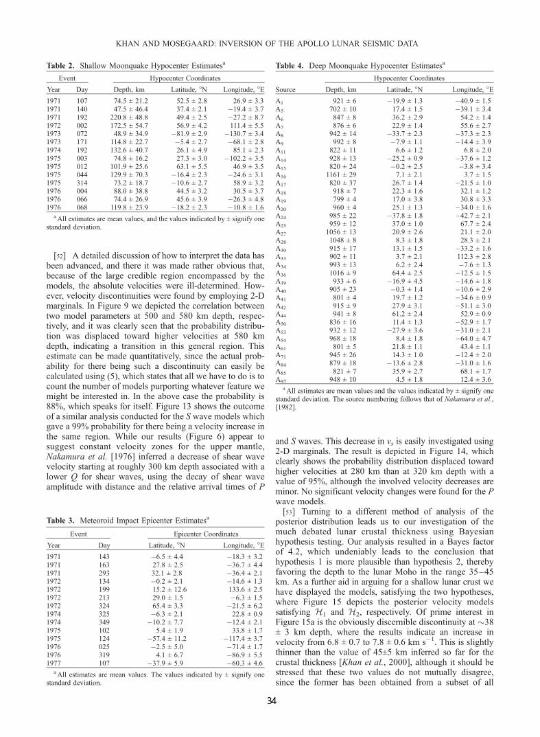
[52] A detailed discussion of how to interpret the data hasbeen advanced, and there it was made rather obvious that,because of the large credible region encompassed by themodels, the absolute velocities were ill-determined. How-ever, velocity discontinuities were found by employing 2-Dmarginals. In Figure 9 we depicted the correlation betweentwo model parameters at 500 and 580 km depth, respec-tively, and it was clearly seen that the probability distribu-tion was displaced toward higher velocities at 580 kmdepth, indicating a transition in this general region. Thisestimate can be made quantitatively, since the actual prob-ability for there being such a discontinuity can easily becalculated using (5), which states that all we have to do is tocount the number of models purporting whatever feature wemight be interested in. In the above case the probability is88%, which speaks for itself. Figure 13 shows the outcomeof a similar analysis conducted for the S wave models whichgave a 99% probability for there being a velocity increase inthe same region. While our results (Figure 6) appear tosuggest constant velocity zones for the upper mantle,Nakamura et al. [1976] inferred a decrease of shear wavevelocity starting at roughly 300 km depth associated with alower Q for shear waves, using the decay of shear waveamplitude with distance and the relative arrival times of P

and S waves. This decrease in vs is easily investigated using2-D marginals. The result is depicted in Figure 14, whichclearly shows the probability distribution displaced towardhigher velocities at 280 km than at 320 km depth with avalue of 95%, although the involved velocity decreases areminor. No significant velocity changes were found for the Pwave models.[53] Turning to a different method of analysis of the

posterior distribution leads us to our investigation of themuch debated lunar crustal thickness using Bayesianhypothesis testing. Our analysis resulted in a Bayes factorof 4.2, which undeniably leads to the conclusion thathypothesis 1 is more plausible than hypothesis 2, therebyfavoring the depth to the lunar Moho in the range 35–45km. As a further aid in arguing for a shallow lunar crust wehave displayed the models, satisfying the two hypotheses,where Figure 15 depicts the posterior velocity modelssatisfying H1 and H2, respectively. Of prime interest inFigure 15a is the obviously discernible discontinuity at �38± 3 km depth, where the results indicate an increase invelocity from 6.8 ± 0.7 to 7.8 ± 0.6 km s�1. This is slightlythinner than the value of 45±5 km inferred so far for thecrustal thickness [Khan et al., 2000], although it should bestressed that these two values do not mutually disagree,since the former has been obtained from a subset of all

Table 2. Shallow Moonquake Hypocenter Estimatesa

Event Hypocenter Coordinates

Year Day Depth, km Latitude, �N Longitude, �E

1971 107 74.5 ± 21.2 52.5 ± 2.8 26.9 ± 3.31971 140 47.5 ± 46.4 37.4 ± 2.1 �19.4 ± 3.71971 192 220.8 ± 48.8 49.4 ± 2.5 �27.2 ± 8.71972 002 172.5 ± 54.7 56.9 ± 4.2 111.4 ± 5.51973 072 48.9 ± 34.9 �81.9 ± 2.9 �130.7 ± 3.41973 171 114.8 ± 22.7 �5.4 ± 2.7 �68.1 ± 2.81974 192 132.6 ± 40.7 26.1 ± 4.9 85.1 ± 2.31975 003 74.8 ± 16.2 27.3 ± 3.0 �102.2 ± 3.51975 012 101.9 ± 25.6 63.1 ± 5.5 46.9 ± 3.51975 044 129.9 ± 70.3 �16.4 ± 2.3 �24.6 ± 3.11975 314 73.2 ± 18.7 �10.6 ± 2.7 58.9 ± 3.21976 004 88.0 ± 38.8 44.5 ± 3.2 30.5 ± 3.71976 066 74.4 ± 26.9 45.6 ± 3.9 �26.3 ± 4.81976 068 119.8 ± 23.9 �18.2 ± 2.3 �10.8 ± 1.6

aAll estimates are mean values, and the values indicated by ± signify onestandard deviation.

Table 3. Meteoroid Impact Epicenter Estimatesa

Event Epicenter Coordinates

Year Day Latitude, �N Longitude, �E

1971 143 �6.5 ± 4.4 �18.3 ± 3.21971 163 27.8 ± 2.5 �36.7 ± 4.41971 293 32.1 ± 2.8 �36.4 ± 2.11972 134 �0.2 ± 2.1 �14.6 ± 1.31972 199 15.2 ± 12.6 133.6 ± 2.51972 213 29.0 ± 1.5 �6.3 ± 1.51972 324 65.4 ± 3.3 �21.5 ± 6.21974 325 �6.3 ± 2.1 22.8 ± 0.91974 349 �10.2 ± 7.7 �12.4 ± 2.11975 102 5.4 ± 1.9 33.8 ± 1.71975 124 �57.4 ± 11.2 �117.4 ± 3.71976 025 �2.5 ± 5.0 �71.4 ± 1.71976 319 4.1 ± 6.7 �86.9 ± 5.51977 107 �37.9 ± 5.9 �60.3 ± 4.6

aAll estimates are mean values. The values indicated by ± signify onestandard deviation.

Table 4. Deep Moonquake Hypocenter Estimatesa

Source

Hypocenter Coordinates

Depth, km Latitude, �N Longitude, �E

A1 921 ± 6 �19.9 ± 1.3 �40.9 ± 1.5A5 702 ± 10 17.4 ± 1.5 �39.1 ± 3.4A6 847 ± 8 36.2 ± 2.9 54.2 ± 1.4A7 876 ± 6 22.9 ± 1.4 55.6 ± 2.7A8 942 ± 14 �33.7 ± 2.3 �37.3 ± 2.3A9 992 ± 8 �7.9 ± 1.1 �14.4 ± 3.9A11 822 ± 11 6.6 ± 1.2 6.8 ± 2.0A14 928 ± 13 �25.2 ± 0.9 �37.6 ± 1.2A15 820 ± 24 �0.2 ± 2.5 �3.8 ± 3.4A16 1161 ± 29 7.1 ± 2.1 3.7 ± 1.5A17 820 ± 37 26.7 ± 1.4 �21.5 ± 1.0A18 918 ± 7 22.3 ± 1.6 32.1 ± 1.2A19 799 ± 4 17.0 ± 3.8 30.8 ± 3.3A20 960 ± 4 25.1 ± 1.3 �34.0 ± 1.6A24 985 ± 22 �37.8 ± 1.8 �42.7 ± 2.1A25 959 ± 12 37.0 ± 1.0 67.7 ± 2.4A27 1056 ± 13 20.9 ± 2.6 21.1 ± 2.0A28 1048 ± 8 8.3 ± 1.8 28.3 ± 2.1A30 915 ± 17 13.1 ± 1.5 �33.2 ± 1.6A33 902 ± 11 3.7 ± 2.1 112.3 ± 2.8A34 993 ± 13 6.2 ± 2.4 �7.6 ± 1.3A36 1016 ± 9 64.4 ± 2.5 �12.5 ± 1.5A39 933 ± 6 �16.9 ± 4.5 �14.6 ± 1.8A40 905 ± 23 �0.3 ± 1.4 �10.6 ± 2.9A41 801 ± 4 19.7 ± 1.2 �34.6 ± 0.9A42 915 ± 9 27.9 ± 3.1 �51.1 ± 3.0A44 941 ± 8 61.2 ± 2.4 52.9 ± 0.9A50 836 ± 16 11.4 ± 1.3 �52.9 ± 1.7A53 932 ± 12 �27.9 ± 3.6 �31.0 ± 2.1A54 968 ± 18 8.4 ± 1.8 �64.0 ± 4.7A61 801 ± 5 21.8 ± 1.1 43.4 ± 1.1A71 945 ± 26 14.3 ± 1.0 �12.4 ± 2.0A84 879 ± 18 �13.6 ± 2.8 �31.0 ± 1.6A85 821 ± 7 35.9 ± 2.7 68.1 ± 1.7A97 948 ± 10 4.5 ± 1.8 12.4 ± 3.6

aAll estimates are mean values and the values indicated by ± signify onestandard deviation. The source numbering follows that of Nakamura et al.,[1982].


Klaus Mosegaard

34

sampled models, namely, those models that additionallyconcur with the constraints imposed by H1. The modelswhich were found to have discontinuities in the depth range50–70 km are displayed in Figure 15b. One might betempted to label these models unphysical, but what isactually apparent here is the nonuniqueness inherent in

the data we are dealing with, which leads to a multitudeof possible models with clearly quite different implicationsfor the lunar crustal velocity structure. The interpretation ofFigure 15b is such that it shows that in order for the MCMCalgorithm to generate models incorporating velocity dis-continuities at depths around 60 km it seems at the same

Figure 13. Two-dimensional marginal S wave velocity distribution depicting the correlation betweensampled velocity parameters at 500 and 580 km depth. The distribution is clearly seen to be translatedtoward higher velocities at a depth of 580 km, indicating the existence of a velocity jump. Ninety-ninepercent of the probability distribution is situated above the equality line.

Figure 14. Two-dimensional marginal S wave velocity distribution depicting the correlation betweensampled velocity parameters at 280 and 320 km depth. The distribution is clearly seen to be translatedtoward higher velocities at a depth of 280 km, indicating the existence of a velocity decrease in thisregion. Ninety-five percent of the probability distribution lies below the equality line.


Klaus Mosegaard

35

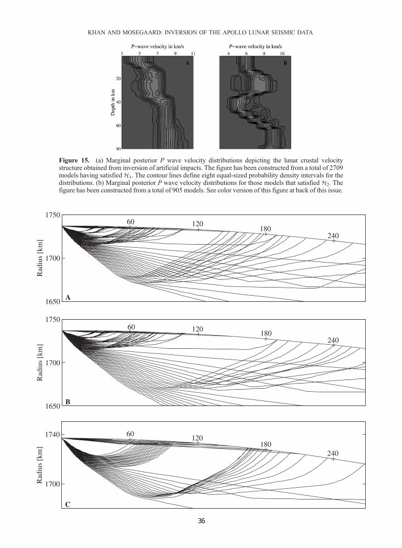
Figure 15. (a) Marginal posterior P wave velocity distributions depicting the lunar crustal velocitystructure obtained from inversion of artificial impacts. The figure has been constructed from a total of 2709models having satisfied H1. The contour lines define eight equal-sized probability density intervals for thedistributions. (b) Marginal posterior P wave velocity distributions for those models that satisfied H2. Thefigure has been constructed from a total of 905 models. See color version of this figure at back of this issue.


Klaus Mosegaard

36

time to have a preference for generating substantial velocitydecreases in the lower crust. Now, the sampling of suchgeologically unsound models could easily have beenrestricted. However, this would have required the introduc-tion of prior information into the inverse problem, whichimplies constraining the numerical system, thereby reducingits nonuniqueness and not exposing the true model varia-bility, which, as noted, was one of the primary motivations

for conducting our reanalysis of the Apollo lunar seismicdata. Moreover, what actually constitutes ‘‘geologicallyunsound’’ features in a model is often debatable given itssubjectivity.[54] Of relevance in assessing Bayesian hypothesis test-

ing as a tool for inferring conclusions is to inquire whetherthe conclusions reached are contingent upon the hypotheses;that is, is the Bayes factor dependent upon the specific

Figure 16. (opposite) Seismic ray paths in the Moon for a surface source. Figures 16a and 16b correspond to the Toksozmodel with velocity discontinuities of 2 km/s and 1 km/s placed at 60 km depth. Figure 16c shows ray paths using thevelocity model obtained here, with a velocity discontinuity of 1 km/s at a depth of 42 km. Where the density of rays is high,focusing of energy has occurred, leading to large amplitudes. Numbers on the lunar surface denote epicentral distance inkilometers.

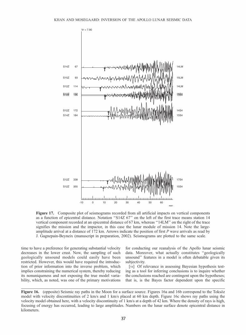
Figure 17. Composite plot of seismograms recorded from all artificial impacts on vertical componentsas a function of epicentral distance. Notation ‘‘S14Z 67’’ on the left of the first trace means station 14vertical component recorded at an epicentral distance of 67 km, whereas ‘‘14LM’’ on the right of the tracesignifies the mission and the impactor, in this case the lunar module of mission 14. Note the large-amplitude arrival at a distance of 172 km. Arrows indicate the position of first P wave arrivals as read byJ. Gagnepain-Beyneix (manuscript in preparation, 2002). Seismograms are plotted to the same scale.


Klaus Mosegaard

37

constraints employed in describing the physical features ofinterest? This is easily verified by simply altering theconstraints. As an example, let us look for discontinuitiesin our models specified according to the following defini-tions:1. Velocity gradients should reach 0.3 km s�1 km�1.

2. The velocity beneath the crust should reach a value of8.0 km s�1.[55] We also extended the depth range in which we seek

the crust-mantle boundary of hypothesis 1, from 35–45 kmto 30–50 km, so as to have the same size as the rangeconsidered in hypothesis 2, but intuitionally searching agreater depth range should just result in an augmentednumber of models satisfying H1. The Bayes factor for thisanalysis is B12 = 7.5, leading to a further increase in theplausibility of H1 relative to H2. This should confirm thereliability of hypothesis testing.[56] In view of the discrepancy between the crustal

thickness estimate presented in this study and the onesobtained earlier, with values ranging from 65 km [Toksozet al., 1972] over 55 km [Toksoz et al., 1974] to 58 km[Nakamura et al., 1982] for the region below the Apollo 12and 14 landing sites, a few comments are merited. (For thesake of completeness, it should be noted that another recentreanalysis of the Apollo lunar seismic data set, althoughusing a different inversion technique, has also resulted in athinner estimate for the crustal thickness [Chenet et al.,2002].) In the study of Toksoz et al. [1972, 1974], amplitudedata and synthetic seismograms were employed in additionto the travel times from the man-made impacts.

[57] Now, amplitude data do provide additional informa-tion on velocity discontinuities, since phenomena such asgeometric focusing, defocusing, and reflection of seismicrays are controlled by velocity gradients. These effects areillustrated in Figures 16a, 16b, and 16c for three differentvelocity models. Figures 16a and 16b depict ray paths inthe crust using the Toksoz model, with velocity disconti-nuities of 2 and 1 km/s situated at 60 km depth, respec-tively. It is clear that in order to focus rays at theappropriate epicentral distance with the Toksoz model soas to obtain the observed large first P wave arrival at adistance of 172 km (see Figure 17), a discontinuity of 2 km/s is needed, which is probably difficult to realize. Figure16c, on the other hand, shows that it is indeed possible to fitthe same data by a model corresponding to the onepresented in this study, including a 1 km/s discontinuityat a depth of 42 km.[58] The positive velocity discontinuity will, of course,

produce a multiplicity in the travel time curve correspondingto the different arrivals, like the refracted first arrival, thedirect arrival, and, if present, any reflected arrivals. Thereforethe presence of any later P wave arrivals will provide addi-tional evidence for velocity gradients or discontinuities insidethe Moon. In the studies of Toksoz et al. [1972, 1974], laterarrivals as well as surface reflected phases were reportedlyidentified in the seismograms and used to further evince theexistence of a high-velocity discontinuity. However, thenotorious coda seen on lunar seismograms, produced byintense scattering, obscures secondary and all later arrivingphases, thereby severely hampering their identification. This

Figure 18. The SIVB 15 impact, 29 July 1971, as recorded at ALSEP 12 (LP) at a distance of 356 km.Traces start at 20 h 58 min 50.5 s. Ground motion is given in du. Here X and Y represent the horizontalcomponents of ground motion, and Z corresponds to vertical motion. The two peaks immediately after thearrow are clearly visible on the Z component and were identified as noise by Toksoz et al. [1972]. Aheadof these two pulses the signal itself contains very little noise, and the present authors are therefore moreprone to picking the first arrival at the arrow, rather than 5 s later. While the Y component does not revealanything, the X component contains a signal (indicated by the arrow) that corresponds to the one on thevertical component.


Klaus Mosegaard

38

does not necessarily mean that none of the purported secon-dary arrivals are real. Some of them may truly representreflected and converted phases from some interface, butothers may quite possibly be due to side scattering(Y. Nakamura, personal communication, 2001).[59] The calculation of theoretical seismograms defines a

more definitive approach, since these can be directly com-pared to their observed equivalents. The computation ofsynthetic seismograms is mostly dependent on the velocitystructure but, of course, also depends on the seismic sourceand the response of the seismometer. For details of howseismograms were computed the reader is referred to Toksozet al. [1972]. Figure 6 of that manuscript, in particular, showsa comparison of observed and synthetic seismograms, and itis apparent even from a first look that discrepancies are

present, especially when considering the impact recorded atan epicentral distance of 356 km. Concerning this particularseismogram, the authors state that (p. 497): ‘‘. . .the first twopeaks of the observed seismograms are noise pulses and canbe clearly identified as such in unfiltered seismograms.’’However, an independent review of this event, by the presentauthors (see Figure 18) does not qualify the two pulses asnoise, but rather as the start of the signal, which, of course,leaves the synthetics and thereby the velocity model used inderiving these questionable.[60] Having said this, one should be aware that the act of

using uncertain data, in the sense of those discussed herewhen solving inverse problems, should be cautioned, sincethe probable inconsistency with which, as an example,secondary later arrivals have been read can lead to biasing

Figure 19. Map of the lunar nearside showing the four Apollo stations as well as deep and shallowmoonquake epicenters taken from Tables 2 and 4, respectively. The white dots on the face of the Moondenote the four stations. Black dots indicate deep moonquakes, and open circles denote shallowmoonquakes. On the rim of the Moon are additionally located three white dots indicating the location ofthe shallow moonquakes on the lunar farside. The white square on the right near the lunar equator showsthe location of the lone farside deep moonquake.


Klaus Mosegaard

39

of the final result, as it is succinctly stated by Tarantola[1987]:....With such kinds of data, it is clear that the subjectivityof the scientist plays a major role. It is indeed the case,whichever inverse method is used, that results obtained bydifferent scientists (for instance for the location of ahypocenter) from such data sets are different. Objectivitycan only be attained if the data redundancy is greatenough that differences in data interpretation amongdifferent observers do not significantly alter the modelsobtained.[61] In having performed a relocalization of all events,

except the artificial impacts, we will briefly discuss thespatial distribution of the natural seismic events. The currentdepth distribution (50–220 km depth) of shallow moon-quakes confirms earlier evidence suggesting the uppermantle to be tectonically active, implying that this regionof the Moon is the only zone in the lunar interior wheretectonic stresses thought to arise from thermal contractionand expansion are high enough to cause mechanical failure[Nakamura et al., 1979]. When the epicenters are drawn onthe lunar surface, some shallow moonquakes appear tooccur, now as then, on the edges of impact basins, whichhad led to the suggestion that they were correlated [Naka-mura et al., 1979] (see Figure 19). However, because of thelimited number of detected events, the statistical signifi-cance of this correlation must be considered inconclusive.[62] Concerning the deep moonquakes, it was observed

in earlier studies [Lammlein et al., 1974; Lammlein, 1977;Nakamura et al., 1982] that their source regions clusteredwithin seismic belts. Two deep belts were identified byLammlein et al. [1974], one belt extending ENE to WSWand another belt extending south. In addition, Nakamura etal. [1982] discerned two more belts in the NW quadranttrending W and WNW. The present distribution seems moreto define a main SW to NE trending belt extending fromsource A24 at 37.8�S and 42.7�W to A85 at 35.9�N and68.1�E, comprising 60% of the events investigated here andlying on an arc of a great circle (see Figure 19). This belt is�250 km in width and 3800 km in length as measured onthe lunar surface. The linear trends inferred earlier in theNW quadrant are less conspicuous with the present distri-bution. The only farside moonquake observed to date,situated at 3.7�N and 112.3�E, most clearly presents anisolated, well-located source of moonquake activity anddoes not appear to be part of the main NE to SW trendingbelt as previously noted [Lammlein et al., 1974]. Thecurious lack of moonquake activity in the SE quadrantwas also observed earlier and was ascribed as being dueto the presence of a localized high attenuation zone oralternatively may simply be due to the absence of deepmoonquakes beneath this mostly highland region [Naka-mura et al., 1982].[63] As concerns the depth distribution of deep moon-

quakes, we have found that 16 events, corresponding toalmost 50%, fall in the narrow range from 850 to 950 km.

7. Conclusion

[64] In this paper we have presented a detailed analysis ofa general inverse problem as is constituted by the inversionof the Apollo lunar seismic data. This was done by using a

MCMC sampling algorithm, that is, by performing a ran-dom walk in a multidimensional model space that combinesprior information with information from measurements andfrom the theoretical relationship between data and modelparameters. Input to the algorithm were random modelsgenerated according to the prior distribution and the like-lihood function. As output we assimilated random realiza-tions of the posterior distribution, which contains all theinformation about the parameterized physical system deriv-able from available sources.[65] We furthermore gave examples of how to investigate

the models comprising the complex posterior distribution ina statistical fashion, using credible intervals, 2-D marginals,and Bayesian hypothesis testing. Common to all of them isthe notion of conjuring up questions relating to any partic-ular property of our interest, like the depth of a particulardeep moonquake, for instance. All models exhibit anexample of this property, and it may turn out that all ofthem provide the same value for it, in which case we wouldsay that the depth of this moonquake is well-constrained bydata. On the other hand, it might also happen that all modelsend up giving different answers to that question, thusrendering this feature ill-determined. Whatever the partic-ular method, the point to note here is that within theprobabilistic formulation of the general inverse problem,doing statistics is an all important asset which provides uswith a clear probabilistic answer.[66] It was also shown that because of the large credible

intervals containing 99% of the probability distribution, theabsolute velocities were not very well-determined. Two-dimensional marginals, on the other hand, could be used toinvestigate the correlation between any two parameters,shedding light on the presence of velocity changes, dis-continuities, and the like. Moreover, Bayesian hypothesistesting was shown to be a very informative tool in providingevidence for the relative plausibility between any twohypotheses concerning features of interest. The advantageof using this form of hypothesis testing to examine a set ofmodels as to certain features was made obvious. Instead ofhaving to a priori constrain the system in certain ways fromthe outset, which means having to run the algorithm againwith different sets of prior information, we chose to invokeas few prior constraints as possible so as to facilitate thecomparison between any two hypotheses in order to gaugewhich particular feature is most probable given data andprior information. We specifically employed Bayesianhypothesis testing to distinguish between a thin and a thicklunar crust, which resulted in a Bayes factor Bij of 4.2,clearly favoring a thinner crust with a thickness around38 km.

8. Future Work

[67] Finally, we would like to touch on the matter alludedto earlier regarding the sampling of P and S wave velocities.Let us consider the following two relations governing thewave velocities as a function of the material parameters:

vp ¼

ffiffiffiffiffiffiffiffiffiffiffiffiffiffiffiffiffiffiffikþ 4=3m

r

s; ð9Þ


Klaus Mosegaard

40

vs ¼ffiffiffimr

r: ð10Þ

From these two equations it is immediately apparent that theparameters vp and vs considered in this study are notindependent when considered in terms of the elasticconstants describing the medium. This raises the interestingproblem of inverting for these parameters instead of thewave velocities using the same arrival time data set, sincethe inherent dependency that is here brought out wouldprobably result in narrower distributions.

[68] Acknowledgments. We are grateful to Yosio Nakamura for aconstructive review of this paper. An anonymous reviewer is also thankedfor comments. Stimulating and highly informative discussions with AlbertTarantola concerning this study and inverse problems in general are muchappreciated by the first author. Finally, we would like to extend ourgratitude to Jeannine Gagnepain-Beyneix for making available Figures 17and 18.

ReferencesBarnett, V., and T. Lewis, Outliers in Statistical Data, John Wiley, NewYork, 1984.

Bernardo, J., and A. Smith, Bayesian Theory, John Wiley, 586 pp., NewYork, 1994.

Chenet, H., J. Gagnepain-Beyneix, and P. Lognonne, A new geophysicalview of the Moon, Lunar Planet. Sci., XXXIII, abstract 1684, 2002.

Duennebier, F., and G. Sutton, Thermal moonquakes, J. Geophys. Res., 79,4351, 1974.

Goins, N., A. Dainty, and M. Toksoz, Seismic energy release of the Moon,J. Geophys. Res., 86, 378, 1981a.

Goins, N., A. Dainty, and M. Toksoz, Lunar seismology: The internalstructure of the Moon, J. Geophys. Res., 86, 5061, 1981b.

Good, I., The interface between statistics and philosophy of science, Stat.Sci., 3, 386, 1988.

Hampel, F., P. Rousseeuw, E. Ronchetti, andW. Stabel,Robust Statistics: TheApproach Based on Influence Functions, John Wiley, New York, 1986.

Khan, A., K. Mosegaard, and K. Rasmussen, A new seismic velocity modelfor the Moon from a Monte Carlo inversion of the Apollo lunar seismicdata, Geophys. Res. Lett., 27, 1591, 2000.

Khan, A., and K. Mosegaard, New information on the deep lunar interiorfrom an inversion of lunar free oscillation periods, Geophys. Res. Lett.,28, 1791, 2001.

Kovach, R., and J. Watkins, Apollo 17 seismic profiling—Probing the lunarcrust, Science, 180, 1063, 1973.

Koyama, J., and Y. Nakamura, Focal mechanism of deep moonquakes,Proc. Lunar Planet. Sci. Conf. 11th, 1855, 1980.

Lammlein, D., Lunar seismicity and tectonics, Phys. Earth Planet. Inter.,14, 224, 1977.

Lammlein, D., G. Latham, J. Dorman, Y. Nakamura, and M. Ewing, Lunarseismicity, structure and tectonics, Rev. Geophys., 12, 1, 1974.

Latham, G., M. Ewing, F. Press, and G. Sutton, Apollo Passive SeismicExperiment, Science, 165, 241, 1969.

Latham, G., et al., Seismic data from man-made impacts on the Moon,Science, 170, 620, 1970.

Latham, G., M. Ewing, F. Press, G. Sutton, J. Dorman, Y. Nakamura,M. Toksoz, D. Lammlein, and F. Duennebier, Passive Seismic Experi-ment, in Apollo 16 Preliminary Science Report, NASA Spec. Publ., NASASP-315, sec. 9, 29 pp., 1972.

Loudin, M., Structural-compositional models of the lunar interior, M.S.thesis, Pa. State Univ., Univ. Park, 1979.

Mosegaard, K., Resolution analysis of general inverse problems throughinverse Monte Carlo sampling, Inverse Problems, 14, 405, 1998.

Mosegaard, K., and A. Tarantola, Monte Carlo sampling of solutions toinverse problems, J. Geophys. Res., 100, 12,431, 1995.

Nakamura, Y., HFT events: Shallow moonquakes?, Phys. Earth Planet.Inter., 14, 217, 1977.

Nakamura, Y., A1 moonquakes: Source distribution and mechanism, Proc.Lunar Planet. Sci. Conf. 9th, 3589, 1978.

Nakamura, Y., Shallow moonquakes: How they compare with earthquakes,Proc. Lunar Sci. Conf. 11th., 1847, 1980.

Nakamura, Y., Seismic velocity structure of the lunar mantle, J. Geophys.Res., 88, 677, 1983.

Nakamura, Y., D. Lammlein, G. Latham, M. Ewing, J. Dorman, F. Press,and M. Toksoz, New seismic data on the state of the deep lunar interior,Science, 181, 49, 1973.

Nakamura, Y., J. Dorman, F. Duennebier, M. Ewing, D. Lammlein, andG. Latham, High-frequency lunar teleseismic events, Proc. Lunar Sci.Conf. 5th, 2883, 1974a.

Nakamura, Y., G. Latham, D. Lammlein, M. Ewing, F. Duennebier, andJ. Dorman, Deep lunar interior inferred from recent seismic data, Geo-phys. Res. Lett., 1, 137, 1974b.

Nakamura, Y., F. Duennebier, G. Latham, and H. Dorman, Structure of thelunar mantle, J. Geophys. Res., 81, 4818, 1976.

Nakamura, Y., G. Latham, H. Dorman, A. Ibrahim, J. Koyama, andP. Horvath, Shallow moonquakes: Depth, distribution and implicationsas to the present state of the lunar interior, Proc. Lunar Planet. Sci. Conf.10th, 2299, 1979.

Nakamura, Y., G. Latham, and J. Dorman, How we processed Apollo lunarseismic data, Phys. Earth Planet. Inter., 21, 218, 1980.

Nakamura, Y., G. Latham, J. Dorman, and J. Harris, Passive Seismic Ex-periment long-period event catalog, Final Version, 1969 day 202–1977day 273, Galveston Geophys. Lab. Contrib. 491, 314 pp., Univ. of Tex.at Austin, 1981.

Nakamura, Y., G. Latham, and J. Dorman, Apollo Lunar Seismic Experi-ment—Final summary, J. Geophys. Res., 87, A117, 1982.

Sellers, P., Seismic evidence for a low-velocity lunar core, J. Geophys. Res.,97, 11,663, 1992.

Tarantola, A., Inverse Problem Theory, 613 pp., Elsevier Sci., New York,1987.

Tarantola, A., and B. Valette, Inverse problems: Quest for information,J. Geophys., 50, 159, 1982.

Toksoz, M., Geophysical data and the interior of the Moon, Annu. Rev.Earth Planet. Sci., 2, 151, 1974.

Toksoz, M., et al., Velocity structure and properties of the lunar crust,Moon, 4, 490, 1972.

Toksoz, M., A. Dainty, S. Solomon, and K. Anderson, Structure of theMoon, Rev. Geophys., 12, 539, 1974.

��

A. Khan and K. Mosegaard, Department of Geophysics, Niels BohrInstitute for Astronomy, Physics and Geophysics, University of Copenha-gen, Juliane Maries Vej 30, 2100 Copenhagen O, Denmark. ([email protected]; [email protected])


Klaus Mosegaard

41

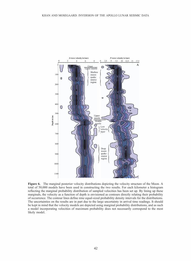
Figure 6. The marginal posterior velocity distributions depicting the velocity structure of the Moon. Atotal of 50,000 models have been used in constructing the two results. For each kilometer a histogramreflecting the marginal probability distribution of sampled velocities has been set up. By lining up thesemarginals, the velocity as a function of depth is envisioned as contours directly relating their probabilityof occurrence. The contour lines define nine equal-sized probability density intervals for the distributions.The uncertainties on the results are in part due to the large uncertainty in arrival time readings. It shouldbe kept in mind that the velocity models are depicted using marginal probability distributions, and as sucha model incorporating velocities of maximum probability does not necessarily correspond to the mostlikely model.

42


Figure 10. Sampled deep moonquake hypocenter coordinates showing the spatial distribution of quakesin the lunar interior. Figures 10a–10c display all sampled hypocenter coordinates for each deepmoonquake source region from a number of different viewpoints. Since the individual source regionscontain a cluster of many thousand samples, which are indvidually not distinguishable, Figure 10ddepicts the distribution of sampled hypocenter coordinates for the lone farside moonquake, A33, forenhancement. Figures 10a–10c also contain a central sphere with a radius of 500 km, which wasincluded so as to enhance illustration of the spatial distribution of the moonquakes and is not meant tosignify a lunar core. In Figure 10c we are viewing down on the lunar north pole, and the only farsidemoonquake observed to date, A33, lying just over the eastern limb, is clearly visible. Crosses denoteseismic stations.

43


Figure 15. (a) Marginal posterior P wave velocity distributions depicting the lunar crustal velocitystructure obtained from inversion of artificial impacts. The figure has been constructed from a total of2709 models having satisfied H1. The contour lines define eight equal-sized probability density intervalsfor the distributions. (b) Marginal posterior P wave velocity distributions for those models that satisfiedH2. The figure has been constructed from a total of 905 models.

44


Documents

An inquiry into the lunar interior: A nonlinear inversion ...jupiter.ethz.ch/~akhan/amir/Research_files/JGR2002.pdf · An inquiry into the lunar interior: A nonlinear inversion of