An Individual Tree-Based Automated Registration of …josh.yosh.org/publications/Lee et al 2016 - An individual tree... · An Individual Tree-Based Automated Registration of Aerial

An Individual Tree-Based Automated Registration of Aerial Images to Lidar Data in a Forested Area

Jun-Hak Lee, Gregory S. Biging, and Joshua B. Fisher

Abstract In this paper, we demonstrate an approach to align aerial images to airborne lidar data by using common object features (tree tops) from both data sets under the condition that conventional correlation-based approaches are challenging due to the fact that the spatial pattern of pixel gray-scale values in aerial images hardly exist in lidar data. We extracted tree tops by using an image processing technique called extended-maxima transfor-mation from both aerial images and lidar data. Our approach was tested at the Angelo Coast Range Reserve on the South Fork Eel River forests in Mendocino County, California. Although the aerial images were acquired simultaneously with the lidar data, the images had only approximate exposure point locations and average flight elevation information, which mimicked the condi-tion of limited information availability about the aerial images. Our results showed that this approach enabled us to align aerial images to airborne lidar data at the single-tree level with reason-able accuracy. With a local transformation model (piecewise lin-ear model), the RMSE and the median absolute deviation (MAD) of the registration were 9.2 pixels (2.3 meters) and 6.8 pixels (1.41 meters), respectively. We expect our approach to be applicable to fine scale change detection for forest ecosystems and may serve to extract detailed forest biophysical parameters.

IntroductionIn forestry, there have been numerous attempts to combine lidar and aerial images to obtain further information and create information-rich products in high spatial resolution (e.g., species identification (Holmgren et al., 2008; Ke et al., 2010; Puttonen et al., 2009), fuel mapping (Mutlu et al., 2008; García et al., 2011), habitat modeling (Hartfield et al., 2011; Estes et al., 2010), land cover classification (Antonarakis et al., 2008; Tooke et al., 2009)). However, the major problem that continues to arise is image rectification, particularly when automated (Leckie et al., 2003; McCombs et al., 2003; Suárez et al., 2005). The rectification of photographic and lidar data is an essential prerequisite to make better use of both systems (Habib et al., 2005; Schenk and Csathó, 2002). The registration of different datasets requires common fea-tures, which are used to geometrically align multiple images. Traditional procedures employ a manual selection of common control points from two datasets for the registration (Habib et al., 2004). However, these manual approaches can be subjec-tive and labor intensive. Also, they may identify a limited number of usable points with poor spatial distribution so that the overall registration accuracy is not guaranteed (Liu et al., 2006). Automated procedures for common feature extraction

are able to cope with some of the limitations of manual pro-cedures (Kennedy and Cohen, 2003). There have been various studies about automatic image registration techniques (Zitova and Flusser, 2003). In brief, techniques for identifying control points are divided into two categories: area-based methods and feature-based methods (Kennedy and Cohen, 2003). Area-based methods (using pixel intensity) have the advantage of easy implementation and no preprocessing requirement for feature extraction. In addition, the resulting control points are evenly distributed over the image so that more robust registra-tion can be performed (Liu et al., 2006; Zitova and Flusser, 2003). However, area-based methods may not be applicable to rectifying aerial images and lidar data because the spatial patterns of pixel grey-scale values (optical reflectance) in aerial images hardly exist in the raw lidar point data. Con-versely, feature-based methods use salient features rather than direct intensity values so that feature-based methods are more suitable for multi-sensor analysis (i.e., lidar and aerial images in this study) (Zitova and Flusser, 2003). For feature-based methods, distinctive and detectable common objects (features) should be extracted from both datasets. The common features selected for the registration greatly influ-ence subsequent registration procedures. Hence, it is crucial to decide on the appropriate common features to be used for the registration between the datasets (Habib et al., 2004). Since there is nothing in common at the level of raw data (discrete points in lidar and pixels in aerial image), additional processing is required to extract the common features (Schenk and Csathó, 2002). Habib et al. (2005) used linear features for matching. Mitishita and others (2008) extracted the centroids of rectangular building roofs as common features. De Lara and others (2009) proposed corner and edge detection methods for automatic integration of digital aerial images and lidar data. Abayowa et al. (2015) registered optical aerial imagery to a lidar point cloud. However, these methods cannot be readily applied to non-urban forested areas that do not have built-up objects (e.g., buildings, roads and roofs) for the registration (Li et al., 2013).

Common features for the registration ideally should be distinct, evenly distributed over the entire image, and eas-ily detectable. In forested areas, trees are usually detectable objects and spread across areas of interest so that there is great potential in utilizing dominant trees as control points. Several studies have verified the feasibility of automated tree apex detection in both aerial images and lidar data. For aerial images, different approaches have been made to detect tree tops; local maxima (Dralle and Rudemo, 1997; Pouliot et al., 2002; Wulder et al., 2000), image binarization (Dralle and Rudemo, 1996; Walsworth and King, 1998), scale analy-sis (Brandtberg and Walter, 1998; Pouliot and King, 2005),

Jun-Hak Lee is with the Department of Landscape Architecture, University of Oregon, Eugene, OR 97403 ([email protected]).

Gregory S. Biging is with the Department of Environmental Science, Policy and Management, University of California, Berkeley, CA 94720.

Joshua B. Fisher is with the Jet Propulsion Laboratory, California Institute of Technology, Pasadena, CA 91109.

Photogrammetric Engineering & Remote SensingVol. 82, No. 9, September 2016, pp. 699–710.

0099-1112/16/699–710© 2016 American Society for Photogrammetry

and Remote Sensingdoi: 10.14358/PERS.82.9.699

Photogrammetric engineering & remote SenSing September 2016 699

08-16 September Peer Reviewed.indd 699 8/24/2016 9:17:20 AM

template matching (Pollock, 1996; Sheng et al., 2001), Markov random fields (Descombes and Pechersky, 2006), and marked point processes (Perrin et al., 2004). Ke and Quackenbush (2011) and Larsen et al. (2011) summarized and explained dif-ferent methods to detect tree tops and delineate tree canopy boundaries from aerial images. The majority of these studies used the fact that bright peaks in the image correspond to treetops because of the higher level of solar illumination (Ke and Quackenbush, 2011). Also, for lidar data, there have been extensive studies to detect individual trees by using a Digital Surface Model (DSM) from lidar data (Chen et al., 2006; Jing et al., 2012; Kankare et al., 2015; Persson et al., 2002; Popescu and Wynne, 2004; Solberg et al., 2006).

The objective of this study is to register aerial images to lidar data by means of automated tree top detection for use as control points. More specific aims are: (1) detecting individ-ual tree top locations from lidar data and aerial images by us-ing image processing techniques (morphological operations), (2) finding corresponding point pairs between aerial images and lidar data, (3) aligning aerial images to lidar data, and (4) mosaicking aligned multiple aerial images to lidar data.

Although we conducted this study with forestry applica-tions in mind, we intended to detect only relatively large trees for the aerial image registration to lidar data. In addition, we developed this approach to perform correctly when minimal information about the aerial images (flight path, time, and flight height) is available. Thus, the images without Inertial Measurement Unit (IMU) and Differential Global Positioning System (DGPS) data can be registered to the lidar data using our approach. The proposed method is specifically designed for a structurally heterogeneous forested area with complex local distortion, which is challenging for automated multi-source data integration at high spatial resolution.

Study Area and Remote Sensing Data

Study SiteThis study was conducted at the Angelo Coast Range Reserve (39° 45' N; 123° 38' W; 430 to 1,290 m elevation), part of the University of California Natural Reserve System on the South Fork Eel River in Mendocino County, California. The Angelo Coast Range Reserve is composed of old conifer forests, domi-nated by Douglas Fir (Pseudotsuga menziesii) and Redwood (Sequoia sempervirens) trees and mixed-hardwood, includ-ing several oaks (Lithocarpus densiflorus, Quercus agrifolia, Quercus kelloggi), California bay (Umbellularia californica), and mandrone (Arbutus menziesii) (Kotanen, 2004). Average temperatures range from 16°C to 31°C with annual average precipitation of 216 cm/yr (http://www.ucnrs.org/reserves/angelo-coast-range-reserve.html). We studied a subset of the larger 180 km2 of the South Fork Eel River watershed for which lidar and aerial photos were acquired by the National Center for Earth-surface Dynamics.

DataThe lidar data and aerial photography were acquired simul-taneously on the same airplane on 29 June 2004. Figure 1 shows an overview of the subset area by means of the DSM generated from the lidar data and the flight lines with approx-imate photo center locations. Lidar data were recorded using the Airborne Laser Swath Mapping (ALSM) system. The ALSM system is comprised of an Optech, Inc. model 1233 Airborne Laser Terrain Mapper (ALTM) unit, Inertial Measurement Unit (IMU) and Differential Global Positioning System (DGPS). The laser pulse frequency is 33 kHz, and the swath width is 20 degrees per half angle. The datasets include the first and last returns for x, y, z coordinates, intensity value, and GPS time for the first and last returns. The point density of the lidar points was 2.64 returns/m2. The vertical accuracy of the point data was reported as 15 to 20 cm for the ALTM system. Digital aerial images were acquired by an optical 3-Charge-Coupled Device (CCD) digital multispectral camera (Redlake MASD, Inc., model MS4100). The image frame size is 1920 (cross-

track) × 1080 (along-track) for two million pixels with three visible bands (Red, Green, Blue). The 28 mm focal length lens has a 25 cm × 25 cm ground sample distance at 600 m flying height above ground. The aerial images were taken from a near vertical viewpoint. Al-though aerial images were acquired simultaneously with the lidar data, the images had only approximate exposure points and average flight elevation data in Esri shape file format. We were not able to acquire the detailed IMU and DGPS data.

MethodsThe work flow of our method is de-picted in Figure 2. In this study, we extracted tree tops as common con-trol points from the aerial images and the lidar DSM by morphological operations, and we used tree top points from the lidar DSM, which is georeferenced, as reference points. Then, feature matching between the two data sets was performed to find an initial matching of control points. Because we used point fea-tures as control points, we applied a point pattern matching method

Figure 1. Overview of the study area (Digital Surface Model generated from lidar data and the flight lines with approximate photo center locations).

700 September 2016 Photogrammetric engineering & remote SenSing


to find corresponding pairs. In order to cope with radial relief displacement problems in the aerial images, only the subset of the detected points (near the principal point) was used for the initial matching. Also, the search range for the refer-ence points (from the lidar DSM) was limited based on camera

orientation information such as aerial image center coordi-nates, flight directions, and flight heights. Once the initial referencing was conducted, exterior orientation parameters of the aerial image were estimated coarsely. Based on the initial estimation, we iteratively refined the exterior orientation by back-projecting tree top locations from lidar data onto the aerial images to search and expand corresponding pairs. We registered aerial images onto lidar data by a piecewise-linear transformation with the previously paired control points. After we registered each aerial image, adjacent aerial images were combined by means of automatic image mosaicking pro-cedures. We used MATLAB® to conduct this study and Esri’s ArcGIS® 10.2 for visualization of different data sets.

Lidar Data Analysis

Digital Surface Model (DSM)Tree top detection is typically performed using a canopy height model (CHM), which is calculated by subtracting the DEM from the DSM. However, in this study, we used the DSM rather than the CHM because the DSM is a representation of surface shape of the real world (not modified by subtracting ground elevation). In order to detect tree tops by morphologi-cal operations, discrete lidar points needed to be converted to a regular grid. First, a regular grid was laid out and the maximum elevation point within each cell was assigned as a cell value to derive the top of the vegetation surface (Popescu and Wynne, 2004). Then, linear interpolation was performed

to create the DSM. The cell size was set to 0.25 m because we intended to process the DSM with aerial photo-graphs that had a ground sample distance of 20 to 30 cm so we want these pixel sizes to be equivalent.

Smoothing the DSM It is common to smooth the surface before detecting tree tops because smoothing reduces irrelevant surface fluctuations, which can cause inac-curate tree top detection (Wang et al., 2004; Wulder et al., 2000; Pouliot et al., 2002; Leckie et al., 2005). In this study, we used a 2D Gauss-ian filter to smooth the DSM. With coarse scales (large smoothing filter sizes), small trees could be missed and overlapping trees could be mistakenly detected as a single tree. In contrast, with fine scales (small smoothing filter sizes), large branch-es or other variances within a crown could be falsely detected as tree tops (Figure 3 shows the effect of different filter sizes for tree top detection with a lidar DSM).

We used an empirical approach to select an optimum filter size. In this study it was more important to detect distinctive tree tops rather than to identify all tree tops. Also, falsely detected tree tops were more problematic than omission errors (missed trees). However, it was required to extract enough tree tops (control points) to construct an accu-rate transformation equation. Hence, the filter size had to be as small as possible to maximize the number of

Figure 2. Workflow of rectification method.

Figure 3. An example of the effect of different filter sizes for tree top detection with lidar DSM; w: Gaussian filter width (in meters); (+) represents a detected tree top location.



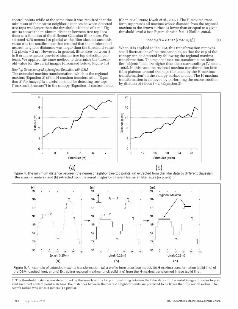
control points while at the same time it was required that the minimum of the nearest neighbor distances between detected tree tops was larger than the threshold distance of 3 m1. Fig-ure 4a shows the minimum distance between tree top loca-tions as a function of the different Gaussian filter sizes. We selected 4.75 meters (19 pixels) as the filter size, because this value was the smallest one that ensured that the minimum of nearest neighbor distances was larger than the threshold value (12 pixels = 3 m). However, in general, filter sizes between 3 to 5 or more meters provided similar tree top detection pat-terns. We applied the same method to determine the thresh-old value for the aerial images (discussed below; Figure 4b)

Tree Top Detection by Morphological Operation with DSMThe extended-maxima transformation, which is the regional maxima (Equation 2) of the H-maxima transformation (Equa-tion 3) for image f, is a useful method for detecting tree tops (“maximal structure”) in the canopy (Equation 1) surface model

(Chen et al., 2006; Kwak et al., 2007). The H-maxima trans-form suppresses all maxima whose distance from the regional maxima to the crown surface is lower than or equal to a given threshold level h (see Figure 5b with h = 1) (Soille, 2003).

EMAXh(f) = RMAX[HMAXh (f)] (1)

When it is applied to the DSM, this transformation removes small fluctuations of the tree canopies, so that the cap of the canopy can be detected by following the regional maxima transformation. The regional maxima transformation identi-fies “objects” that are higher than their surroundings (Vincent, 1993). In this case, the regional maxima transformation iden-tifies plateaus around tree tops (flattened by the H-maxima transformation) in the canopy surface model. The H-maxima transformation is achieved by performing the reconstruction by dilation of f from f − h (Equation 2):

Figure 4. The minimum distance between the nearest neighbor tree top points: (a) extracted from the lidar data by different Gaussian filter sizes (in meters), and (b) extracted from the aerial images by different Gaussian filter sizes (in pixels)

Figure 5. An example of extended-maxima transformation: (a) a profile from a surface model, (b) H-maxima transformation (solid line) of the DSM (dashed line), and (c) Extracting regional maxima (thick solid line) from the H-maxima transformed image (solid line).

1. The threshold distance was determined by the search radius for point matching between the lidar data and the aerial images. In order to pre-vent incorrect control point matching, the distances between the nearest neighbor points are preferred to be larger than the search radius. The search radius was set as 3 meters (12 pixels).



HMAXh(f) = Rfδ(f – h) (2)

where f is an input image, h a nonnegative scalar, R a recon-struction function, and δ a dilation operator. In this study, f is the DSM and Rf

δ(f – h) is defined as the geodesic dilation of f with respect to f – h, and iterated until stability is reached (Soille, 2003).

The regional maxima transformation is performed by subtracting the dilation of f – h from f (Equation 3) and this transformation identifies regional maxima as 1 and all others as 0.

RMAX(f) = f – Rfδ(f – h) (3)

When h is too small, the results are too sensitive to small fluctuations of the DSM. In this case the h-value creates too many false tree tops. On the other hand, when the h value is too large, the extended maxima transformation cannot detect tree tops properly. Based on results from pilot tests, we set the h-value to 1 meter, which was not too sensitive to the fluc-tuation of DSM and small enough to detect tips of the canopy surface as tree tops. Because the result of extended maxima transformation was a region (connected cells), the point with maximum elevation value in the region was marked as a tree top location. Figure 5 illustrates an example of the extended-maxima transformation.

Aerial Image AnalysisFor an individual tree, the tree top is typically the brightest part because the peak is more likely to be directly illuminated from different sun angles than the edge parts for the convex shape of a tree; adjacent trees will shade the edges of their neighbor (Wulder, 2003). Therefore, reflectance value (image intensity) can represent relative height within an individual tree. The same method as described for extracting individual tree tops from the DSM with the lidar data was applied to extract tops of individual trees from aerial images with reflec-tance values.

Grayscale Intensity SurfaceThe aerial images used in this study have three visible bands (red, green, blue). Although multispectral information is use-ful for object classification, morphological analysis is appli-cable to only single band images. Accordingly, we converted color images into panchromatic images (intensity) by the “rgb2gray” function in Matlab. Once grayscale intensity im-ages were created, these images were processed with the same method we used for the DSM from the lidar data.

Smoothing Aerial ImagesWe applied Gaussian filtering to reduce image noise and re-move in-canopy fluctuations (Pouliot et al., 2002). As we did for the lidar DSM, the optimal smoothing parameters were em-pirically selected to maximize detecting distinctive tree tops and to minimize falsely detected tree tops. Figure 4b shows the minimum distance between tree top locations by the dif-ferent Gaussian filter sizes. We selected 23 pixels as the filter size, because this was the smallest value that ensured that the minimum of the nearest neighbor distances was larger than the threshold value (12 pixels).

Tree Top Detection by Morphological Operation with Aerial ImagesThe extended-maxima transformation was applied to identify groups of pixels that represent the tip of tree crowns. Then, the tree apex was detected by selecting the maximum inten-sity value within a certain group of pixels. An h-value was set to 1 in grayscale images (0 to 255), which was decided by sim-ilar pilot tests as previously conducted. We utilized bright-ness gradient information to detect tree tops. However, not all of the brighter spots were associated with tree apexes. Thus,

we separated vegetation pixels from non-vegetation pixels and excluded non-vegetation pixels because falsely detected tree tops from non-vegetation pixels may cause problems in finding a correct pair of tree tops (as control points). Because the peak points from non-vegetation regions were brighter than the peak points from vegetation regions, we applied a threshold value for excluding non-vegetation points (Dralle and Rudemo, 1996; Pitkänen, 2001; Pouliot and King, 2005). By using the histogram of brightness values of the detected peak locations, we plotted a histogram and determined the threshold value as 130. Accordingly, only the points whose pixel brightness values were lower than 130, were classified as tree tops and used as control points.

Initial Transformation EstimationIt is well understood that in aerial photographs relief dis-placement increases as radial distance from the principal point increases (Wolf and Dewitt, 2000). Accordingly, there is only a negligible amount of relief displacement near the principal point. Because lidar data are already geo-rectified, feature points (tree tops) detected from lidar DSM are also geo-registered. Tree top point features that were detected from the center (near the principal point) of the aerial images have a negligible amount of displacement as well. Hence, a geometric transformation (linear conformal transformation in this study which equals rotation, scaling and translation) was applicable to align two sets of points. The major prob-lem in estimating a transformation equation to align two data sets was finding correct matching pairs. In order to solve this problem, we used the fact that the transformation equation estimated from corresponding pairs yields the highest number of matched pairs, while the transformation equations from non-corresponding pairs have a limited number of matched pairs; the concept of this approach is similar to the random sample consensus (RANSAC) method (Fischler and Bolles, 1981). We applied a linear conformal transformation com-posed of four parameters: s, θ, tx, and ty, where s was a scale factor, δ the rotation angle, and tx and ty the translation along the x and y directions, respectively. We used conformal trans-formation rather than affine transformation. The transforma-tion employed in this step was described by Equation 4 (Wolf and Dewitt, 2000).

θ θx

y

t

tscos ssin

ssin scosLiDAR

LiDAR

x

y

=

+

− θ θ

x

yphoto

photo (4)

To begin our procedure one of the N (N-1)/2 tree top points pairs were selected from the center region of the aerial image and two tree top points were randomly selected from the lidar DSM (N is the number of detected tree top points from the aeri-al images). Then, using Equation 4 we solved for s, θ, tx, and ty. Once the relationship was established it was possible to trans-late other tree top points in the middle region of the aerial images into the lidar DSM which had a geo-rectified coordinate system. Then, the nearest points between the transformed points (from the aerial image to the lidar data) and the tree top points from the lidar DSM were paired. If the distance between the two points from the two data sources was within a given threshold (12 pixels), the points were considered as “matched points.” We counted the number of “matched points” for each of all possible combination of point pairs. When the correct corresponding pair of points was selected, the estimated transformation equation provided the maximum number of “matched points.”

Figure 6 demonstrates an example of the initial transforma-tion estimation. It started with selecting a pair of points (P16 and P19) from the center region of the aerial image (Figure 6a). Then, a pair of points was selected from the detected tree



tops from the lidar DSM. (Figure 6b shows the search area in the lidar data). In order to find the correct corresponding pair, we counted the number of “matched points” for each of all possible combination of point pairs.

Figure 6c shows a case of selecting incorrect correspond-ing pairs. When incorrect corresponding points (P59 and P71) were selected, the estimated conformal transformation provided only a small number of “matched points” (six cases in this example). Conversely, when a correct correspond-ing pair of points (P59 - P61) was selected, we obtained the highest number of matched pairs (23 cases in this example) (Figure 6d).

In order to speed up the search procedure, we reduced the search sets by setting up threshold values for transformation angles and scales. The point pairs that are out of the range of the threshold values were excluded when finding matched pairs. Also, these threshold values helped to prevent false cor-responding pairs. The angle thresholds were calculated from

the flight line data. The flight line data had the approximate orientation of each image so that the angle thresholds are set to the flight line orientation angle ±5 degrees. The scale threshold is estimated from the average flight height. The range of threshold height was set to ±200 m of the average flight height. Then, the scale threshold range was calculated from the focal length and the average flight height. We in-tended to expand the threshold value of the orientation angle and the scale, but we were able to find sufficient numbers of corresponding point pairs using the initial threshold values. Therefore, we did not need to expand threshold values.

Once the initial matching control point pairs were found, we used the Direct Linear Transformation (DLT) method, which is applicable to non-calibrated camera models, to de-termine initial approximate internal and external orientation elements. The DLT models the transformation between the 2D image plane and 3D object space as a linear function and the basic projective equations are as follow:

Figure 6. An example of initial transformation estimation: (a) Tree tops detected near the center of aerial image, (b) tree tops detected from lidar DSM, (c) an example of few matched pairs when the transformation equation is estimated by using trees 59 and 71 in the lidar image and trees 16 and 19 in the aerial image, and (d) an example of the maximum number of matched pairs when the transformation equa-tion is estimated by using trees 59 and 61 in the lidar image and trees 16 and 19 in the aerial image. White circles (O) indicate correctly matched control points, and white crosses (X) indicate incorrectly matched control points. The coordinates of the X and Y axes are in meters.



x xL X L Y L Z L

L X L Y L Z

y yL X L Y L

p p p

p p p

p p

+ =+ + ++ + +

+ =+ +

δ

δ

1 2 3 4

9 10 11

5 6

1

77 8

9 10 11 1

Z L

L X L Y L Zp

p p p

++ + +

(5)

where Xp, Yp, and Zp are the object space coordinates of the point; x and y are the image coordinates; δx and δy are nonlin-ear systematic errors; L1 to L11 are 11 DLT parameters that can be interpreted in terms of the interior and exterior orientation of the image (Abdel-Aziz and Karara, 1971).

Iterative Matched Point Expansion and Exterior Orientation RefinementAlthough we used geometric relations of the points between the two data sets for finding corresponding pairs between aerial images and the lidar DSM for initial matching, this approach was only applicable for the part of the image near the principal point. As the radial distance increases the relief displacement increases and the geometric relations of points were not consistent. Consequently, it was necessary to consider the relief displacement of aerial images for finding corresponding pairs by the nearest point matching scheme (the nearest points between two data sources were paired if the distance between two points was smaller than a threshold value). The initial coarse external orientation parameters for the aerial image estimated using the feature points from the lidar data had 3D information (x, y, z). Then, we applied the backward projection of the 3D feature points from the lidar DSM (in object space) into the aerial images (in image space) for searching and adding corresponding pairs. The backward projection was conducted using the collinearity equation (Equation 6) (Wolf and Dewitt, 2000).

x x x cr X X r Y Y r Z Zr X X r Y Y

c c c

c c

+ = −− + − + −− + − +

δ 011 12 13

31 32

( ) ( ) ( )( ) ( ) rr Z Z

y y y cr X X r Y Y r Z Zr X X

c

c c c

c

33

021 22 23

31

( )

( ) ( ) ( )( )

−

+ = −− + − + −− +

δrr Y Y r Z Zc c32 33( ) ( )− + −

(6)

where Xc, Yc, and Zc, are object coordinates of the camera location, and x0 and y0 are image coordinates of the principal point, c is the principal distance, δx and δy are nonlinear systematic errors, and r11, r12, … r33 are the camera orientation parameters estimated from the previous steps.

Once we performed the backward projection, the nearest point matching scheme could be used to find corresponding pairs between the two data sets. Based on newly added con-trol point pairs, camera orientation parameters were updated and used for the next step. At each step, the radius (a distance from the principal point) of the search area is gradually in-creased until all the points in the image were used.

Image RectificationOnce the feature correspondence between the lidar data (mas-ter image) and the aerial images was established, the mapping function should be determined for image registration (Zitova and Flusser, 2003). In order to establish the mapping function, the type of the mapping function needs to be selected and the parameters for the function should be estimated. Models of mapping functions can be divided into two broad groups; global and local transformation models. For global transfor-mation models, the model parameters are the same for the entire image so that they are inappropriate for handling vari-ous local distortions. In contrast, local transformation models can have different model parameters, which depict local distortions across the whole image (Zitova and Flusser, 2003). Because the aerial images are acquired over heterogeneous

mixed forests that consist of tall conifer trees and steep topo-graphic slopes, the aerial images have various local geometric distortions. Thus, in this study, we employed a local trans-formation model to determine the mapping function. More specifically, we applied a piecewise linear mapping, which decomposes the whole image into triangular facets, and then we used local mapping functions to model the local geometric distortions (Goshtasby, 1986; Liu et al., 2006). We constructed a Delaunay triangulation to decompose the input image by us-ing the extracted control points, and we rectified the image by estimating the transformation of each triangular facet. In addi-tion, we employed three global transformation models (affine, 2nd, and 3rd order polynomial) for the purpose of comparison.

Multi-Frame MosaickingMosaicking combines several image frames into a single composite image to cover a large area (Kerschner, 2001). Aerial photographs are a common source for creating photo mosaics because multiple frames are acquired to cover a large area (Afek and Brand, 1998). Because we rectify multi-frame images, which cover a part of the study area, we also perform image mosaicking to combine the rectified aerial images. In mosaicking two adjacent images, it is necessary to decide how to process the overlapping areas. In most cases, a seam line (cutline) is defined between two images and the overlapping regions are blended to create a seamless mosaic (Afek and Brand, 1998). In this study, we decomposed each frame into triangular facets which was constructed by common control points. Accordingly, each triangle facet had different trans-formation functions based on the control points. Then, the whole mapping function was acquired by piecing triangular regions together. Because the image mosaicking combined multiple images into one large image, adjacent image frames had overlapping areas. We used the proximity of the trian-gular facet to the center of the images in order to determine which image frame would be selected for each triangular region. The proximity was calculated by finding the nearest image center point from the vertices of the triangle.

Evaluation of Image Registration AccuracyBecause we used the lidar data as master image for the reg-istration, we used the treetop points detected using morpho-logical operations from the lidar data as reference points. For evaluating the accuracy of the registration, we applied the Leave-One-Out Cross-Validation (LOOCV), which is a com-mon cross-validation method. Cross-validation is a statisti-cal method of evaluating and comparing the performance of learning algorithms by dividing data into two groups (one is for learning or training and the other is for validation) (Stone, 1974). The LOOCV is a special case of the k-fold cross-valida-tion method, which split the data into k mutually exclusive subsets of equal (or almost equal) size (Kohavi, 1995). In k-fold cross-validation, a single subset is retained for validation, and the remaining k-1 subsets are used as training data. The training and validation are performed iteratively (k times) so that each of the k subsets is used exactly once (Refaeilzadeh and Tang, 2009). The LOOCV uses only one observation for validation and uses the remaining observations as training data. In other words, the LOOCV is a k-fold cross validation, where k is equal to the size of the dataset. Accordingly, we retained one control point from the pool as a validation point and estimated a geometric transformation function using the remaining points. Then, we applied this transformation func-tion to locate the retained control point. In each iteration, we calculated the residual (distance) between the true point and the estimated point. By using the calculated residuals, we calculated the maximum x-residual, the maximum y-residual, the total RMSE, the median absolute deviation (MAD), and the standard deviation (SD) of the residuals to evaluate the



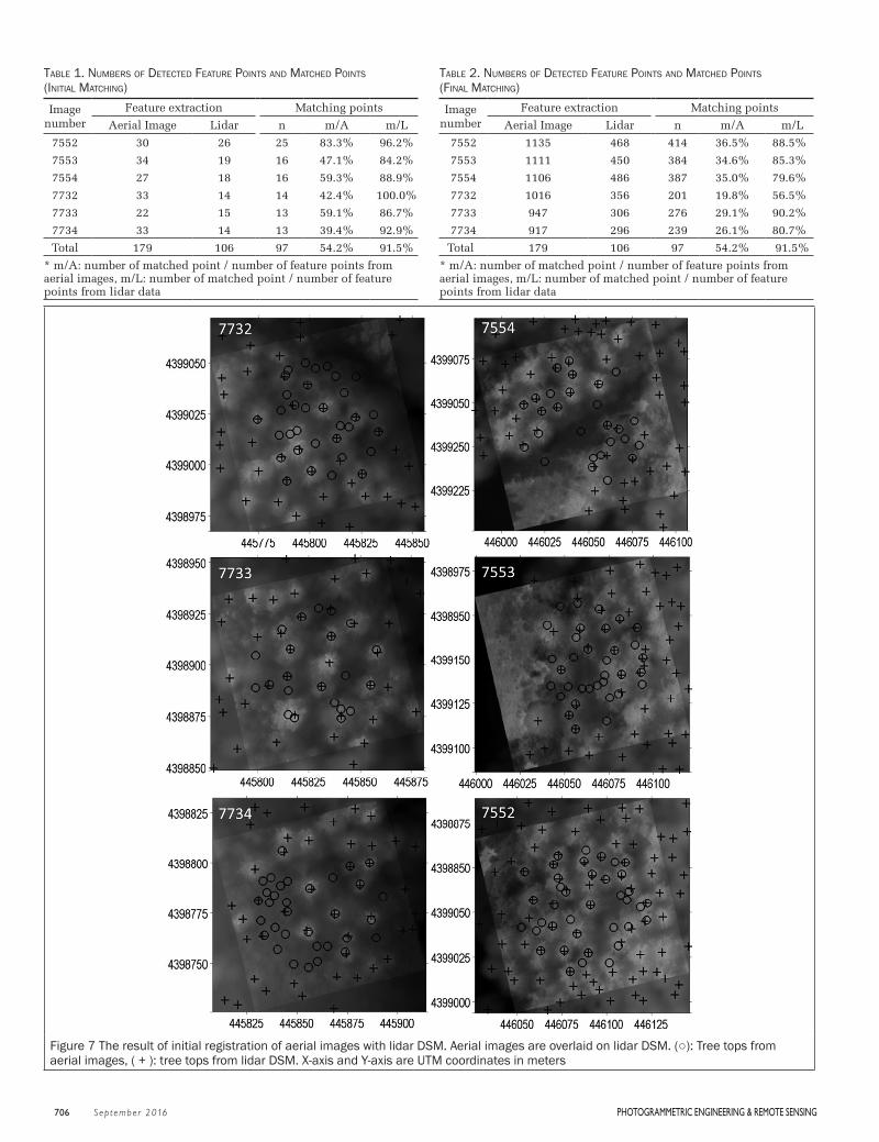
table 1. numbers oF DetecteD Feature Points anD matcheD Points (initial matching)

Image number

Feature extraction Matching points

Aerial Image Lidar n m/A m/L

7552 30 26 25 83.3% 96.2%

7553 34 19 16 47.1% 84.2%

7554 27 18 16 59.3% 88.9%

7732 33 14 14 42.4% 100.0%

7733 22 15 13 59.1% 86.7%

7734 33 14 13 39.4% 92.9%

Total 179 106 97 54.2% 91.5%

* m/A: number of matched point / number of feature points from aerial images, m/L: number of matched point / number of feature points from lidar data

table 2. numbers oF DetecteD Feature Points anD matcheD Points (Final matching)

Image number

Feature extraction Matching points

Aerial Image Lidar n m/A m/L

7552 1135 468 414 36.5% 88.5%

7553 1111 450 384 34.6% 85.3%

7554 1106 486 387 35.0% 79.6%

7732 1016 356 201 19.8% 56.5%

7733 947 306 276 29.1% 90.2%

7734 917 296 239 26.1% 80.7%

Total 179 106 97 54.2% 91.5%

* m/A: number of matched point / number of feature points from aerial images, m/L: number of matched point / number of feature points from lidar data

Figure 7 The result of initial registration of aerial images with lidar DSM. Aerial images are overlaid on lidar DSM. (○): Tree tops from aerial images, ( + ): tree tops from lidar DSM. X-axis and Y-axis are UTM coordinates in meters



registration errors. Also, we used these four indexes to com-pare the differences between transformation models: affine, 2nd order polynomial, 3rd order polynomial, and piecewise linear model.

ResultsTree Top Detection and MatchingTable 1 shows the number of feature points extracted from six aerial images and lidar data in the initial matching step. In this study, the aerial images had more feature points than the lidar data. Accordingly, the matched points between two data-sets were mainly limited by the feature points obtained from the lidar data. Although some images had fewer correspond-ing points than the others, all the images had enough control points to estimate initial exterior orientation parameters. Fig-ure 7 shows the results of initial alignment of the six images. Although the initial match was conducted from the small cen-tral region of the aerial image, we were able to conduct initial alignment for all images. Table 2 lists the number of feature points obtained in automatic tree top detection from both data sets and the number of corresponding points by the iterative matched point expansion method. We detected an average of 1,038 points per image and an average of 394 points from the lidar DSM from the equivalent area. Overall, 80 percent of the feature points from the lidar data were matched to corresponding points for the transformation. However, only 30.5 percent of the feature points from the aerial images were paired with the corresponding points from the lidar data. This was mainly because small deciduous trees had less distinc-tive apexes in the canopy. Consequently, those fluctuations were removed by the image smoothing. While the number of trees detected from the different aerial images range from 917 to 1,135, the number of detected trees from image #7552 to #7554 was larger than that of detected trees from image #7732 to #7734 (Table 2). We suspect two major factors affected the differences between images. First, the densities of detectable trees were not the same for different images, and the areas with lower densities had less detectable trees than the others. Second, the time of day that the image was taken might cause the differences in the shapes and patterns of shadows. For the test images, trees on the eastern slope (#7732, #7733, and #7734) were less detectable than the others (#7752, #7753, and #7754) because those trees were located on the shaded slope (the images were acquired in the afternoon hours).

Transformation Model ComparisonWe applied a local transformation model (piecewise linear model) to register the aerial images to the lidar data. In addi-tion, we used three global transformation models (affine, 2nd order polynomial, and 3rd order polynomial) for the purpose of comparison. We employed the LOOCV method to evaluate the accuracy of the registration between the aerial images and lidar data. Table 3 shows the result of accuracy assessment by using five different registration error indexes: maximum x-residual, maximum y-residual, total RMSE, median absolute deviation (MAD), and standard deviation of the overall residu-al. All the registration error indexes verify that the piecewise linear model produced the smallest registration errors. Be-cause a global transformation model cannot properly handle local image deformation, a global transformation model has relatively larger registration errors than a local transformation model. Therefore, when we applied a piecewise linear model, the total RMSE of the residual was 9.21 pixels (2.3 meters), and MAD was 6.81 pixels (1.41 meters). The maximum X direc-tional errors were larger than the maximum Y directional errors, because the aerial images were wider in the X (1,920 pixels) direction than in the Y direction (1,080 pixels). As

the distance from the principal point increases, the relief displacement also increases. Therefore, it was more likely to have a larger number of points which were further away from the principal point in the X direction than in the Y direction.

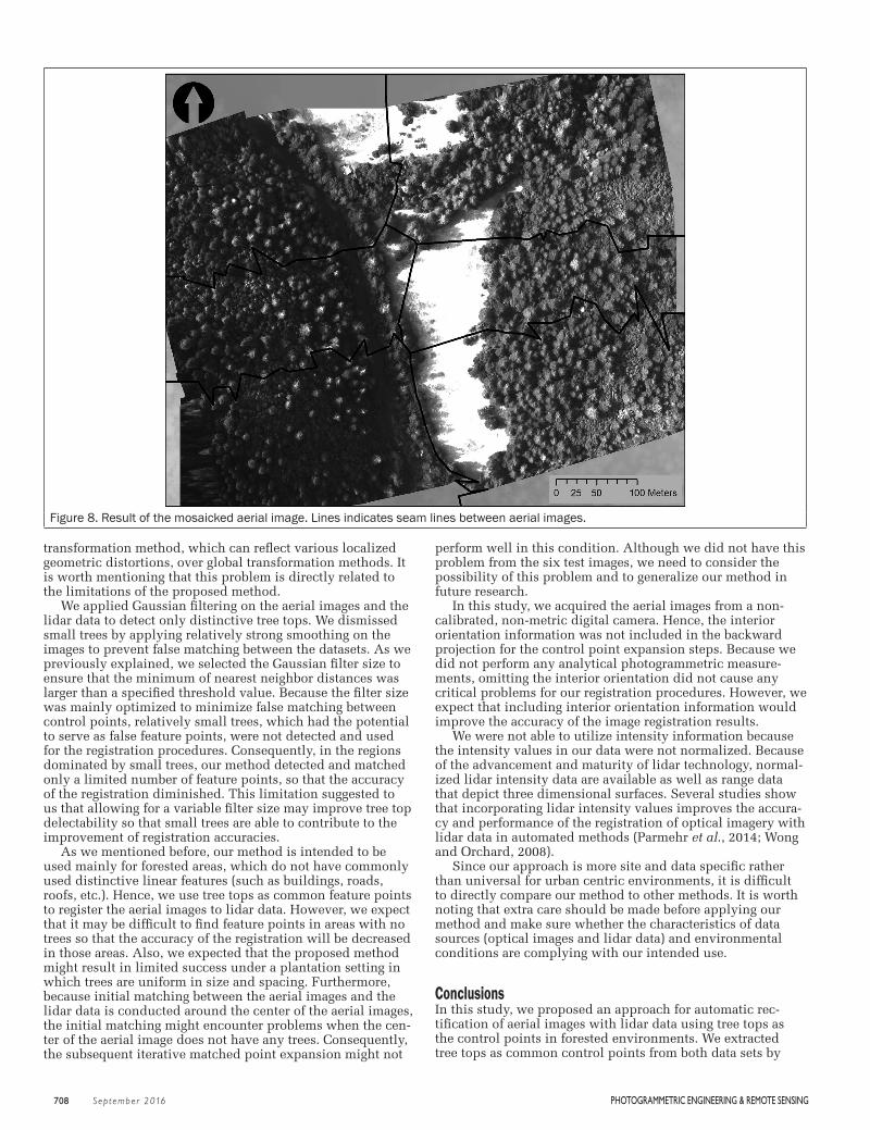
Image MosaickingWe mosaicked six overlapping images together by using com-mon control points that were shared by adjacent images. We visually examined the transitional areas between images for comparisons. Compared to the outcome of the simple prox-imity based image mosaicking method, the result of image mosaicking using common control points showed seamless transitions around the seam lines (Figure 8). The quality of the seamless transition between images was better when enough common control points existed. However, when the overlapping area had sparse common points, the seam lines were more noticeable because of misalignment between the neighboring images. In this study, the test site included open areas without trees. Thus, these open areas have sparsely distributed control points so that the transitions between the images around the open areas were less smooth than the tran-sitions between the images around the densely forested areas.

DiscussionAutomatic registration of multi-source remote sensing is not an easy task because it needs to handle various radiometric characteristics, image resolution, sensor orientation, and local deformation in the registration procedures: feature identifica-tion, feature matching, spatial transformation, and interpola-tion (Zitova and Flusser, 2003). Combining multi-spectral images and lidar data is useful because the complementary characteristics of lidar and aerial photography enable us to more fully utilize the advantages of both systems (Habib et al., 2005; Schenk and Csathó, 2002). However, these multi-source data sets have very different radiometric characteris-tics, so it is challenging to identify and match corresponding features to register the two datasets by automated procedures. In this study, we employed trees (generally tall trees), which are abundant over forested areas, as common control points for the feature-based registration. In addition, we utilized the geometric configuration of the detected tree tops to find initial corresponding point pairs between the aerial images and the lidar data, which had very different radiometric charac-teristics. The results indicated that tree tops were able to be used to register high spatial resolution multi-source remote sensing data in forested areas. Also, as we expected, the piecewise linear transformation was more accurate than other polynomial and affine transformation methods. However, the accuracy differences between the piecewise linear transfor-mation and other polynomial transformation methods were less pronounced than expected. We suspect some regions do not have enough control points for accurate registration, and this problem might diminish the advantage of using a local

table 3. comParison between moDels anD accuracy inDexes (in meters)Transformation

ModelMax X

ResidualMax Y

ResidualTotal RMSE MAD

S.D. of the residual

Affine 15.08 13.51 4.88 3.77 2.42

2nd order polynomial

13.33 8.54 2.94 1.87 1.78

3rd order polynomial

11.65 8.05 2.48 1.70 1.42

Piecewise linear

10.12 6.27 2.30 1.41 1.41



transformation method, which can reflect various localized geometric distortions, over global transformation methods. It is worth mentioning that this problem is directly related to the limitations of the proposed method.

We applied Gaussian filtering on the aerial images and the lidar data to detect only distinctive tree tops. We dismissed small trees by applying relatively strong smoothing on the images to prevent false matching between the datasets. As we previously explained, we selected the Gaussian filter size to ensure that the minimum of nearest neighbor distances was larger than a specified threshold value. Because the filter size was mainly optimized to minimize false matching between control points, relatively small trees, which had the potential to serve as false feature points, were not detected and used for the registration procedures. Consequently, in the regions dominated by small trees, our method detected and matched only a limited number of feature points, so that the accuracy of the registration diminished. This limitation suggested to us that allowing for a variable filter size may improve tree top delectability so that small trees are able to contribute to the improvement of registration accuracies.

As we mentioned before, our method is intended to be used mainly for forested areas, which do not have commonly used distinctive linear features (such as buildings, roads, roofs, etc.). Hence, we use tree tops as common feature points to register the aerial images to lidar data. However, we expect that it may be difficult to find feature points in areas with no trees so that the accuracy of the registration will be decreased in those areas. Also, we expected that the proposed method might result in limited success under a plantation setting in which trees are uniform in size and spacing. Furthermore, because initial matching between the aerial images and the lidar data is conducted around the center of the aerial images, the initial matching might encounter problems when the cen-ter of the aerial image does not have any trees. Consequently, the subsequent iterative matched point expansion might not

perform well in this condition. Although we did not have this problem from the six test images, we need to consider the possibility of this problem and to generalize our method in future research.

In this study, we acquired the aerial images from a non-calibrated, non-metric digital camera. Hence, the interior orientation information was not included in the backward projection for the control point expansion steps. Because we did not perform any analytical photogrammetric measure-ments, omitting the interior orientation did not cause any critical problems for our registration procedures. However, we expect that including interior orientation information would improve the accuracy of the image registration results.

We were not able to utilize intensity information because the intensity values in our data were not normalized. Because of the advancement and maturity of lidar technology, normal-ized lidar intensity data are available as well as range data that depict three dimensional surfaces. Several studies show that incorporating lidar intensity values improves the accura-cy and performance of the registration of optical imagery with lidar data in automated methods (Parmehr et al., 2014; Wong and Orchard, 2008).

Since our approach is more site and data specific rather than universal for urban centric environments, it is difficult to directly compare our method to other methods. It is worth noting that extra care should be made before applying our method and make sure whether the characteristics of data sources (optical images and lidar data) and environmental conditions are complying with our intended use.

ConclusionsIn this study, we proposed an approach for automatic rec-tification of aerial images with lidar data using tree tops as the control points in forested environments. We extracted tree tops as common control points from both data sets by

Figure 8. Result of the mosaicked aerial image. Lines indicates seam lines between aerial images.



applying a morphological operation and searched the cor-responding points based on the fact that the transformation equation estimated from corresponding pairs yields the high-est number of matched pairs. The test aerial images were suc-cessfully rectified over the lidar DSM data with the automated procedures at single-tree level accuracy.

The main limitation of our approach was in using only tree tops as matching feature points for the registration. Although our approach performed well over the forested area with enough distinctive trees, it would be very difficult to regis-ter the aerial images with lidar data over an area with few or no detectable trees. We need more research to find other corresponding features (other than tree tops) to cope with this problem for future studies. In addition, we assume that brightness maxima in aerial images correspond to tree apex locations (Korpela et al., 2006). However, we suspect that this simplified assumption is one of the major sources of relatively large registration errors. Hence, more rigorous investigations need to be conducted to assess the discrepancies between the tree apex locations and brightness maxima.

We expect the proposed approach will enable us to inte-grate aerial images and lidar data at the individual tree level. Hence, the integrated data sets may serve to extract detailed forest biophysical parameters (vertical and horizontal struc-tures, forest type classification, tree canopy volume, forest stand age, and aboveground biomass) so that more detailed and accurate information will help to expand our understand-ing of forest ecosystem dynamics. In addition, our approach may contribute to fine scale single tree level change detection for forest ecosystems.

AcknowledgmentsWe gratefully acknowledge the use of lidar data sets supplied by Dr. William E. Dietrich and the National Center of Air-borne Laser Mapping (NCALM). The first author was partially funded by the W.S. Rosecrans Fellowship, Environmental Science, Policy, and Management, University of Califor-nia, Berkeley. Dr. Joshua B. Fisher contributed to this paper through work by the Jet Propulsion Laboratory, California Institute of Technology, under a contract with the National Aeronautics and Space Administration.

ReferencesAbdel-Aziz, Y.I., and H.M. Karara. 2015. Direct linear transformation

from comparator coordinates into object space coordinates in close-range photogrammetry, Photogrammetric Engineering & Remote Sensing, 81(2):103–107.

Abayowa, B.O., A. Yilmaz, and R.C. Hardie. 2015. Automatic registration of optical aerial imagery to a LiDAR point cloud for generation of city models, ISPRS Journal of Photogrammetry and Remote Sensing, 106:68–81.

Afek, Y., and A. Brand. 1998. Mosaicking of orthorectified aerial images, Photogrammetric Engineering & Remote Sensing 64(2):115–124.

Antonarakis, A., K. Richards, and J. Brasington, 2008. Object-based land cover classification using airborne LiDAR, Remote Sensing of Environment, 112(6):2988–2998.

Brandtberg, T., and F. Walter, 1998. Automated delineation of individual tree crowns in high spatial resolution aerial images by multiple-scale analysis, Machine Vision and Applications, 11(2):64–73.

Chen, Q., D. Baldocchi, P. Gong, and M. Kelly, 2006. Isolating individual trees in a Savanna woodland using small footprint lidar data, Photogrammetric Engineering & Remote Sensing, 72(8):923–932.

Descombes, X., and E. Pechersky, 2006. Tree crown extraction using a three states Markov Random Field, Rapport de Recherche, RR-5982:14.

Dralle, K., and M. Rudemo, 1996. Stem number estimation by kernel smoothing of aerial photos, Canadian Journal of Forest Research, 26(7):1228–1236.

Dralle, K. 1997. Automatic estimation of individual tree positions from aerial photos, Canadian Journal of Forest Research, 27(11):1728–1736.

Estes, L.D., P.R. Reillo, A.G. Mwangi, G.S. Okin, and H.H. Shugart, 2010. Remote sensing of structural complexity indices for habitat and species distribution modeling, Remote Sensing of Environment, 114(4):792–804.

Fischler, M.A., and R.C. Bolles, 1981. Random sample consensus: A paradigm for model fitting with applications to image analysis and automated cartography, Communications of the ACM, 24(6):381–395

García, M., D. Riaño, E. Chuvieco, J. Salas, and F.M. Danson, 2011. Multispectral and LiDAR data fusion for fuel type mapping using Support Vector Machine and decision rules, Remote Sensing of Environment, 115(6):1369–1379.

Goshtasby, A., 1986. Piecewise linear mapping functions for image registration, Pattern Recognition, 19(6):459–466.

Habib, A., M. Ghanma, and E. Mitishita, 2004. Co-registration of photogrammetric and LIDAR data: Methodology and case study, Revista Brasileira de Cartografia, 56(1):1–13.

Habib, A., M.S. Ghanma, E.A. Mitishita, and E.M. Kim. 2005. Image georeferencing using LIDAR data, Proceedings 2005 IEEE International Geoscience and Remote Sensing Symposium, 2005, IGARSS ’05, 2:1158–1161.

Hartfield, K.A., K.I. Landau, and W.J. van Leeuwen. 2011. Fusion of high resolution aerial multispectral and LiDAR data: Land cover in the context of urban mosquito habitat, Remote Sensing, 3(11):2364–2383.

Holmgren, J., å. Persson, and U. Söderman, 2008. Species identification of individual trees by combining high resolution LiDAR data with multi-spectral images, International Journal of Remote Sensing, 29(5):1537–1552.

Jing, L., B. Hu, J. Li, and T. Noland, 2012. Automated delineation of individual tree crowns from lidar data by multi-scale analysis and segmentation, Photogrammetric Engineering & Remote Sensing, 78(12):1275–1284.

Kankare, V., X. Liang, M. Vastaranta, X. Yu, M. Holopainen, and J. Hyyppä., 2015. Diameter distribution estimation with laser scanning based multisource single tree inventory, ISPRS Journal of Photogrammetry and Remote Sensing, 108:161–171.

Korpela, I., P. Anttila, and J. Pitkänen, 2006. A local maxima method in detecting individual trees in color-infrared aerial photographs, International Journal of Remote Sensing, 27(6):1159–1175 Kwak, D.A., W.K. Lee, J.H. Lee, G.S. Biging, and P. Gong, 2007. Detection of individual trees and estimation of tree height using LiDAR data, Journal of Forest Research, 12(6):425–434.

Ke, Y., and L.J. Quackenbush, 2011. A review of methods for automatic individual tree-crown detection and delineation from passive remote sensing, International Journal of Remote Sensing, 32(17):4725–4747.

Ke, Y., L.J. Quackenbush, and J. Im, 2010. Synergistic use of QuickBird multispectral imagery and LIDAR data for object-based forest species classification, Remote Sensing of Environment 114(6):1141–1154.

Kennedy, R.E., and W.B. Cohen. 2003. Automated designation of tie-points for image-to-image coregistration, International Journal of Remote Sensing, 24(17):3467–3490.

Kerschner, M., 2001. Seamline detection in colour orthoimage mosaicking by use of twin snakes, ISPRS Journal of Photogrammetry and Remote Sensing, 56(1):53–64.

Kohavi, R., 1995. A study of cross-validation and bootstrap for accuracy estimation and model selection, Proceedings of the International Joint Conference on Artificial Intelligence, 14:1137–1145.

De Lara, R., E.A. Mitishita, T. Vogtle, and H.P. Bahr, 2009. Automatic digital aerial image resection controlled by LIDAR data, 3D Geo-Information Sciences, Berlin, Heidelberg: Springer Berlin Heidelberg, pp. 213–234.



Larsen, M., M. Eriksson, X. Descombes, G. Perrin, T. Brandtberg, and F.A. Gougeon, 2011. Comparison of six individual tree crown detection algorithms evaluated under varying forest conditions, International Journal of Remote Sensing, 32(20):5827–5852.

Leckie, D.G., F.A. Gougeon, S. Tinis, T. Nelson, C.N. Burnett, and D. Paradine. 2005. Automated tree recognition in old growth conifer stands with high resolution digital imagery, Remote Sensing of Environment, 94(3):311–326.

Leckie, D., F. Gougeon, D. Hill, R. Quinn, L. Armstrong, and R. Shreenan, 2003. Combined high-density lidar and multispectral imagery for individual tree crown analysis, Canadian Journal of Remote Sensing, 29(5):633–649. Li, N., X. Huang, F. Zhang, and L. Wang, 2013. Registration of aerial imagery and lidar data in desert areas using the centroids of bushes as control information, Photogrammetric Engineering & Remote Sensing, 79(8):743–752.

Liu, D., P. Gong, M. Kelly, and Q. Guo, 2006. Automatic registration of airborne images with complex local distortion, Photogrammetric Engineering & Remote Sensing, 72(9):1049.

McCombs, J.W., S.D. Roberts, and D.L. Evans. 2003. Influence of fusing lidar and multispectral imagery on remotely sensed estimates of stand density and mean tree height in a managed loblolly pine plantation, Forest Science, 49(3):457–466.

Mitishita, E., A. Habib, J. Centeno, A. Machado, J. Lay, and C. Wong, 2008. Photogrammetric and lidar data integration using the centroid of a rectangular roof as a control point, The Photogrammetric Record, 23(121):19–35.

Mutlu, M., S.C. Popescu, C. Stripling, and T. Spencer. 2008. Mapping surface fuel models using lidar and multispectral data fusion for fire behavior, Remote Sensing of Environment,112 (1):274–285.

Parmehr, E.G., C.S. Fraser, C. Zhang, and J. Leach, 2014. Automatic registration of optical imagery with 3D LiDAR data using statistical similarity, ISPRS Journal of Photogrammetry and Remote Sensing 88:28–40.

Perrin, G., X. Descombes, and J. Zerubia, 2004. Tree crown extraction using marked point processes, Proceedings of the European Signal Processing Conference (EUSIPCO), Vienna, Austria.

Persson, A., J. Holmgren, and U. Söderman. 2002. Detecting and measuring individual trees using an airborne laser scanner, Photogrammetric Engineering & Remote Sensing, 68(9):925–932.

Pitkänen, J., 2001. Individual tree detection in digital aerial images by combining locally adaptive binarization and local maxima methods, Canadian Journal of Forest Research, 31(5):832–844.

Pollock, R. 1996. The Automatic Recognition of Individual Trees in Aerial Images of Forests Based On A Synthetic Tree Crown Image Model, Ph.D. Thesis, University of British Columbia.

Popescu, S.C., and R.H. Wynne. 2004. Seeing the trees in the forest: Using lidar and multispectral data fusion with local filtering and variable window size for estimating tree height, Photogrammetric Engineering and Remote Sensing, 70(5):589–604.

Pouliot, D.A., and D.J. King, 2005. Approaches for optimal automated individual tree crown detection in regenerating coniferous forests, Canadian Journal of Remote Sensing, 31:255–267.

Pouliot, D.A., D.J. King, F.W. Bell, and D.G. Pitt, 2002. Automated tree crown detection and delineation in high-resolution digital camera imagery of coniferous forest regeneration, Remote Sensing of Environment, 82(2):322–334.

Puttonen, E., P. Litkey, and J. Hyyppä, 2009. Individual tree species classification by illuminated - shaded area separation, Remote Sensing, 2(1):19–35.

Refaeilzadeh, P., and L. Tang, 2009. Cross-Validation, Encyclopedia of Database Systems (L. Liu and M. Tamer, editors), Boston, Massachusetts, Springer.

Schenk, T., and B. Csathó, 2002. Fusion of lidar data and aerial imagery for a more complete surface description, International Archives of Photogrammetry Remote Sensing and Spatial Information Sciences, 34:310–317.

Sheng, Y., P. Gong, and G.S. Biging. 2001. Model-based conifer-crown surface reconstruction from high-resolution aerial images. Photogrammetric Engineering & Remote Sensing, 67(8):957–965.

Soille, P., 2003. Morphological Image Analysis : Pinciples and Applications, Second edition, Springer, Berlin ;New York.

Solberg, S., E. Naesset, and O.M. Bollandsas, 2006. Single tree segmentation using airborne laser scanner data in a structurally heterogeneous spruce forest, Photogrammetric Engineering and Remote Sensing, 72(12):1369.

Stone, M., 1974. Cross-valedictory choice and assessment of statistical predictions, Journal of the Royal Statistical Society, Series B (Methodological), pp. 111–147.

Suárez, J.C., C. Ontiveros, S. Smith, and S. Snape, 2005. Use of airborne LiDAR and aerial photography in the estimation of individual tree heights in forestry, Computers & Geosciences, 31(2):253–262.

Tooke, T.R., N.C. Coops, N.R. Goodwin, and J.A. Voogt, 2009. Extracting urban vegetation characteristics using spectral mixture analysis and decision tree classifications, Remote Sensing of Environment, 113(2):398–407.

Vincent, L., 1993. Morphological grayscale reconstruction in image analysis: Applications and efficient algorithms, IEEE Transactions on Image Processing, 2(2):176–201.

Walsworth, N.A., and D.J. King, 1998. Comparison of two tree apex delineation techniques, Proceedings of the International Forum on Automated Interpretation of High Spatial Resolution Digital Imagery for Forestry, pp. 93–104.

Wang, L., P. Gong, and G.S. Biging, 2004. Individual tree-crown delineation and treetop detection in high-spatial-resolution aerial imagery, Photogrammetric Engineering & Remote Sensing, 70(3):351–357.

Wolf, P., and B.A. Dewitt, 2000. Elements of Photogrammetry : With Applications in GIS, Third edition, Boston: McGraw-Hill.

Wong, A., and J. Orchard, 2008. Efficient FFT-accelerated approach to invariant optical-LIDAR registration, IEEE Transactions on Geoscience and Remote Sensing, 46(11):3917–3925.

Wulder, M. 2003. Remote Sensing of Forest Environments : Concepts and Case Studies., Boston: Kluwer Academic Publishers.

Wulder, M., K.O. Niemann, and D.G. Goodenough, 2000. Local maximum filtering for the extraction of tree locations and basal area from high spatial resolution imagery, Remote Sensing of Environment, 73(1):103–114.

Zitova, B., and J. Flusser, 2003. Image registration methods: A survey, Image and Vision Computing, 21(11):977–1000.

(Received 14 January 2016; accepted 26 February 2016; final version 28 March 2016)



Documents

An Individual Tree-Based Automated Registration of …josh.yosh.org/publications/Lee et al 2016 - An individual tree... · An Individual Tree-Based Automated Registration of Aerial