Article

Estimating Individual Tree Height and Diameter atBreast Height (DBH) from Terrestrial Laser Scanning(TLS) Data at Plot Level

Guangjie Liu 1,2,3 ID , Jinliang Wang 1,2,3,*, Pinliang Dong 4, Yun Chen 1,2,3 and Zhiyuan Liu 1,2,3

1 College of Tourism and Geographic Sciences, Yunnan Normal University, Kunming 650500, China;guangjiers@gmail.com (G.L.); cqchenyun@126.com (Y.C.); liuzhiyuangis@163.com (Z.L.)

2 Key Laboratory of Resources and Environmental Remote Sensing for Universities in Yunnan,Kunming 650500, China

3 Center for Geospatial Information Engineering and Technology of Yunnan Province, Kunming 650500, China4 Department of Geography and the Environment, University of North Texas, 1155 Union Circle #305279,

Denton, TX 76203, USA; pdong@unt.edu* Correspondence: wang_jinliang@hotmail.com; Tel.: +86-0871-6594-1202

Received: 12 June 2018; Accepted: 2 July 2018; Published: 4 July 2018�����������������

Abstract: Abundant and refined structural information under forest canopy can be obtained by usingterrestrial laser scanning (TLS) technology. This study explores the methods of using TLS to obtainpoint cloud data and estimate individual tree height and diameter at breast height (DBH) at plot levelin regions with complex terrain. Octree segmentation, connected component labeling and randomHough transform (RHT) are comprehensively used to identify trunks and extract DBH of trees insample plots, and tree height is extracted based on the growth direction of the trees. The results showthat the topography, undergrowth shrubs, and forest density influence the scanning range of the plotsand the accuracy of feature extraction. There are differences in the accuracy of the results for differentmorphological forest species. The extraction accuracy of Yunnan pine forest is the highest (DBH: RootMean Square Error (RMSE) = 1.17 cm, Tree Height: RMSE = 0.54 m), and that of Quercus semecarpifoliaSm. forest is the lowest (DBH: RMSE = 1.22 cm, Tree Height: RMSE = 1.23 m). At plot scale, with theincrease of the mean DBH or tree height in plots, the estimation errors show slight increases, andboth DBH and height tend to be underestimated.

Keywords: diameter at breast height (DBH); tree height; random Hough transform; point cloud;terrestrial laser scanning

1. Introduction

Earth’s forests, which cover 30% of the total land area, are dynamic systems that are constantlyin a state of change and drive/respond to the changes taking place in our environment. Tree height,diameter at breast height (DBH) and other forest structure parameters are examples of the importantbasic data recovered from a traditional forest resource survey. They are of great significance for theresearch on forest biomass estimation, forest carbon cycle, carbon flow and global climate change.With the development of remote sensing technology, especially the technology of Light Detection andRanging (LiDAR), many research results have been obtained by using remotely sensed data to extractinformation on forest structure parameters. There are mainly two ways for estimating parametersof forest structure using traditional passive optical imaging: (1) the correlation between foreststructural parameters and spectral information is established by using multi-spectral characteristicsof optical remote sensing data [1,2]; and (2) forest structure parameters are extracted using highspatial resolution image texture features [3–5]. However, due to the complicated structure of forest

Forests 2018, 9, 398; doi:10.3390/f9070398 www.mdpi.com/journal/forests

Forests 2018, 9, 398 2 of 19

canopy cover, atmospheric scattering, and topography, it is difficult for optical remote sensing toprovide accurate information about the vertical distribution of the forests [6,7]. As microwaves canpenetrate dense canopy to obtain information on the branches and trunks below forest canopies,synthetic aperture radar (SAR) is more advantageous than passive optical remote sensing methodsto detect forest structure parameters and biomass [4]. Backscattering mechanism of SAR data [8–10]and interferometric synthetic aperture radar (InSAR) [11,12], polarimetric synthetic aperture radarinterferometry (POLinSAR) [13,14] and polarization coherence tomography (PCT) [15,16] techniquesall have obtained many research results on forest structural parameters. Meanwhile, LiDAR hasbeen intensively applied to the study of forest structural parameters. As space-borne LiDAR canobtain a wide extent of tree height information, it has been applied to studies on large-scale forestbiomass [17,18] and forest canopy height [19,20]. However, the new generation of LiDAR satelliteICESat-2 has not yet been launched, and the lack of spaceborne LiDAR data remains a limitingfactor [21]. Airborne LiDAR has the ability to obtain the vertical structure of large areas of forest, but itusually cannot reflect detailed structural information under tree canopy [22]. Compared with theabove two LiDAR platforms, terrestrial laser scanning (TLS) obtains high density point clouds and canget more detailed information on forest internal structure, including tree location, DBH, tree height,crown width, and other biophysical parameters.

TLS is a laser-based instrument that measures its surroundings using LiDAR for rangemeasurement and precise angular measurements through the optical beam deflection mechanismto derive 3D point observations from the object surfaces [23]. The high-density point cloud dataobtained by TLS is widely used and researched in many fields such as engineering surveys [24,25],Earth sciences [26,27], natural disasters [28–30], coastline erosion [31–33], vegetation monitoring [34,35],and digital terrain mapping [35,36]. In recent years, TLS has been increasingly applied to forest resourcesurveys, forest management and planning [37,38]. Among a variety of forest structural parameters,DBH and tree height are the most important ones obtained in forest resource surveys. They canprovide not only structural parameters of individual trees but also information and data on sampleplot level, which are of great significance for the study of forest carbon storage and biomass estimation.Many researchers have conducted investigations on how to extract DBH, tree height and othersstructural parameters using TLS data efficiently and accurately.

In terms of methodology, the methods for automatically extracting DBH from TLS datamainly include Hough transform [22,39,40], circle fitting algorithm [41–47], and cylinder fittingalgorithm [42,48,49]. Li [40] used the Hough transform method to detect circles on rasterized pointcloud data to estimate DBH and tree height. Liu et al. [22] applied the Hough transform method tonatural forest and plantation in Puer City, China, and concluded that TLS data could be used to extractDBH (RMSE = 2.18 cm, R2 = 0.91). Bienert et al. [41] used a method for fitting circles to extract DBHof trees accurately, and concluded that the tree trunks blocked each other when the tree density washigh, which resulted in the reduction of DBH extraction precision or even led to the unrecognizabletrees. Moskal et al. [38] used the method of cylindrical fitting to extract DBH, with an RMSE of 9.17 cm.The main reasons for the relatively low accuracy were the poor visibility of the scanning station andthe blockage of individual tree trunks. Due to mutual occlusion between the canopy of individualtrees, tree heights extracted from TLS point cloud data are always lower than the measured values [22].The most commonly used method for tree height extraction is to obtain the highest point over theground within a certain range of a single tree, and use the height of the highest cloud point as the treeheight [50]. In order to improve the extraction precision of tree height, most studies have employedthe circle fitting method to determine the growth direction of the tree trunk, and calculate the treeheight along the growth direction of the tree trunk [22,40,51]. In order to improve the efficiency of thealgorithm, the method of extracting DBH based on circle detection or circle fitting needs to rasterizethe point cloud data, which reduces the availability of data and the extraction accuracy [22].

As far as study areas are concerned, most of the studies on the extraction of forest structuralparameters from TLS data focus on plantations of single forest types or a small amount of natural

Forests 2018, 9, 398 3 of 19

forests, and research on tree height and DBH extraction of natural forests from typical tree species in aparticular area is lacking. Also, most of studies on DBH and tree height inversion have been carriedout at scales of individual woods, and studies at scales of forest sample plots with multiple tree speciesand multi-aged forests are still lacking.

To improve the efficiency and accuracy of forest resource surveys, this study explores methods forextracting tree height and DBH at plot level in complex terrain and different sub-wooded environmentsusing TLS data. Four types of dominant forest species (Pinus yunnanensis Franch., Pinus densata Mast.,Picea Mill. & Abies fabri (Mast.) Craib, Quercus semecarpifolia Sm.) are investigated in Shangri-La,northwest of Yunnan, China. Identification of individual trees and extraction of DBH from TLS pointcloud data are implemented by using octree segmentation, connected component labeling (CCL) andRandom Hough Transform (RHT), following the tree growth direction obtained from TLS point data.Based on the extracted individual tree DBH and tree height, the average DBH and the average treeheight are obtained by method of square average.

2. Materials and Methods

2.1. Study Area and Sample Plots

Shangri-La is located in the northwestern part of Yunnan Province, China, the eastern part ofDiqing Tibetan Autonomous Prefecture, between 26◦52′~28◦52′ N and 99◦22′~100◦19′ E with an areaof 11,613 km2. It is one of the largest county-level administrative areas in Yunnan Province (Figure 1).With elevations over 3000 m above sea level in most areas of Shangri-La, the main landform types inthe region are subalpine and alpine, which determines the distribution of cold-temperate coniferousforests and temperate-cool coniferous forests in the area. The area of woodland is 962,159.3 hectares inShangri-La, and total volume of living wood is 133,224,410 m3; the forest coverage rate is 76.00%, andthe forest greening rate is 83.19%. Quercus semecarpifolia, Pinus yunnanensis, Pinus densata, and Picea &Abies fabri (including Abies georgei Orr, Abies delavayi Franch., and Picea likiangensis (Franch.) E.Pritz.)account for 90.8% of the total area of arbors in Shangri-La.

Forests 2018, 9, x FOR PEER REVIEW 3 of 19

a particular area is lacking. Also, most of studies on DBH and tree height inversion have been carried

out at scales of individual woods, and studies at scales of forest sample plots with multiple tree

species and multi-aged forests are still lacking.

To improve the efficiency and accuracy of forest resource surveys, this study explores methods

for extracting tree height and DBH at plot level in complex terrain and different sub-wooded

environments using TLS data. Four types of dominant forest species (Pinus yunnanensis Franch., Pinus

densata Mast., Picea Mill. & Abies fabri (Mast.) Craib, Quercus semecarpifolia Sm.) are investigated in

Shangri-La, northwest of Yunnan, China. Identification of individual trees and extraction of DBH

from TLS point cloud data are implemented by using octree segmentation, connected component

labeling (CCL) and Random Hough Transform (RHT), following the tree growth direction obtained

from TLS point data. Based on the extracted individual tree DBH and tree height, the average DBH

and the average tree height are obtained by method of square average.

2. Materials and Methods

2.1. Study Area and Sample Plots

Shangri-La is located in the northwestern part of Yunnan Province, China, the eastern part of

Diqing Tibetan Autonomous Prefecture, between 26°52′~28°52′ N and 99°22′~100°19′ E with an area

of 11,613 km2. It is one of the largest county-level administrative areas in Yunnan Province (Figure

1). With elevations over 3000 m above sea level in most areas of Shangri-La, the main landform types

in the region are subalpine and alpine, which determines the distribution of cold-temperate

coniferous forests and temperate-cool coniferous forests in the area. The area of woodland is 962,159.3

hectares in Shangri-La, and total volume of living wood is 133,224,410 m3; the forest coverage rate is

76.00%, and the forest greening rate is 83.19%. Quercus semecarpifolia, Pinus yunnanensis, Pinus densata,

and Picea & Abies fabri (including Abies georgei Orr, Abies delavayi Franch., and Picea likiangensis

(Franch.) E.Pritz.) account for 90.8% of the total area of arbors in Shangri-La.

Figure 1. Study Area. Figure 1. Study Area.

Forests 2018, 9, 398 4 of 19

This study used the Leica P40 to acquire high-precision 3D point cloud data. The P40 is Leica’slatest generation 3D laser scanning device for fast, high-density point cloud and panoramic imagecollection. The main performance indicators of the device are shown in Table 1.

Table 1. Main performance indicators of Leica P40.

Indicators Descriptions

Range Accuracy 1.2 mm + 10 ppm

3D position Accuracy 3 mm @ 50 m6 mm @ 100 m

Wavelength 1550nm (invisible); 658 nm (visible)

Scan Rate Up to 1,000,000 points per second

Field-of-View 360◦ (Horizontal); 290◦ (Vertical)

Range and ReflectivityMinimum range: 0.4 m

Maximum range at reflectivity:120 m (8%), 180 m (18%), 270 m (34%)

Range Noise 0.4 mm RMS at 10 m0.5 mm RMS at 50 m

Point cloud data were obtained at three different times (August 2016, July 2017 and September2017) respectively. Because the point cloud data of all trees in a sample plot cannot be acquired by onlyone scanning station, the method of measuring from multiple stations is used in the study. In eachplot, five stations (four stations in some samples) were scanned. One station was in the center of theplot with refined scanning method for 10-min scanning, and panoramic photos were obtained at thesame time. Other stations were set up on the edge of the sample plot with a 5-min scanning. The studyobtained 196 stations of LiDAR point cloud data in 39 forest sample plots (Table 2), which weredistributed in various townships in Shangri-La (Figure 2).

In order to obtain a sufficient amount of data for verification and ensure the reliability of researchresults, we used DBH rulers, Trueyard SP1500H laser rangefinder and steel tape to obtain foreststructural parameters in all 39 forest sample plots (Figure 2). The range of forest plots varies accordingto topography and forest density, but the diameter of each plot is not less than 40 m. With thetopographical conditions permitting, the range of the sample plot was expanded as much as possibleto obtain more data of the tree and to verify the range and accuracy of laser scanning.

Table 2. Number of different types of forest sample plots in the study.

Dominant ForestSpecies

Age ofStand

Number ofSample Plots

Number ofStations

Average Altitude(Unit: m)

Average Slope(Unit: Degree)

Quercussemecarpifolia Sm.

Young 1 5 3892 11.0Middle 2 10 3673 15.0Mature 1 4 3723 30.0

Pinus densataMast.

Young 3 17 3225 16.0Middle 4 20 3210 16.4Mature 2 9 3128 23.5

Pinus yunnanensisFranch.

Young 3 14 2538 19.3Middle 5 25 2692 15.3Mature 8 43 2316 13.9

Picea Mill. &Abies fabri (Mast.)

Craib

Young 2 10 3453 23.3Middle 4 20 3604 13.0Mature 4 19 3680 15.6

Forests 2018, 9, 398 5 of 19Forests 2018, 9, x FOR PEER REVIEW 5 of 19

Figure 2. Forest sample plots in Shangri-La, Yunnan, China.

2.2. Data Acquisition and Processing

The main research process includes point cloud data preprocessing, normalization of point

cloud height, point cloud segmentation, trunk identification, and tree height and DBH extraction. A

flowchart detailing the methods in this study is shown in Figure 3. First, a software, Leica Cyclone,

is used to stitch multi-site point cloud data based on the Leica 4.5″ circular black & white target.

Because there is a lot of redundancy in multi-site point cloud data, the software also is used to deduct

data so that we can reduce the time cost in data processing under the premise of ensuring data

extraction accuracy.

Figure 2. Forest sample plots in Shangri-La, Yunnan, China.

2.2. Data Acquisition and Processing

The main research process includes point cloud data preprocessing, normalization of point cloudheight, point cloud segmentation, trunk identification, and tree height and DBH extraction. A flowchartdetailing the methods in this study is shown in Figure 3. First, a software, Leica Cyclone, is used tostitch multi-site point cloud data based on the Leica 4.5” circular black & white target. Because there isa lot of redundancy in multi-site point cloud data, the software also is used to deduct data so that wecan reduce the time cost in data processing under the premise of ensuring data extraction accuracy.

Forests 2018, 9, 398 6 of 19

Forests 2018, 9, x FOR PEER REVIEW 6 of 19

Figure 3. Flowchart detailing the methods in this study. (a) In order to remove useless data and reduce

the amount of data, point cloud data needs to be preprocessed; (b) Normalization of points height

facilitates the extraction of DBH and tree height; (c) The slicing and segmenting point clouds can

improve the efficiency and accuracy of trunk recognition; (d) According to the trunk position, directly

we extract or fit the DBH. Tree heights are obtained based on the tree growth direction and continuity

detecting.

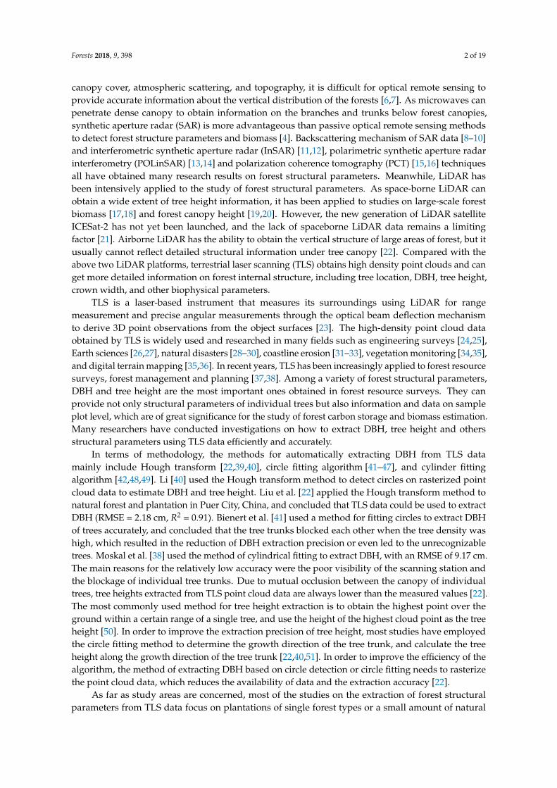
2.2.1. Normalization of Point Cloud Height

A morphological filtering method [52] is used to separate ground points from non-ground

points. The main idea of morphological filtering is to use the corrosion and expansion operations in

mathematical morphology to remove the higher point cloud in the point cloud and keep the lower

point cloud to achieve the purpose of extracting ground points [53]. Ground points are interpolated

and meshed by Inverse Distance Weighting (IDW) method. Finally, using the generated grid of

ground, points heights are normalized to eliminate the difference in tree height caused by differences

in elevation (Figure 4).

Figure 3. Flowchart detailing the methods in this study. (a) In order to remove useless data andreduce the amount of data, point cloud data needs to be preprocessed; (b) Normalization of pointsheight facilitates the extraction of DBH and tree height; (c) The slicing and segmenting point cloudscan improve the efficiency and accuracy of trunk recognition; (d) According to the trunk position,directly we extract or fit the DBH. Tree heights are obtained based on the tree growth direction andcontinuity detecting.

2.2.1. Normalization of Point Cloud Height

A morphological filtering method [52] is used to separate ground points from non-groundpoints. The main idea of morphological filtering is to use the corrosion and expansion operations inmathematical morphology to remove the higher point cloud in the point cloud and keep the lowerpoint cloud to achieve the purpose of extracting ground points [53]. Ground points are interpolatedand meshed by Inverse Distance Weighting (IDW) method. Finally, using the generated grid ofground, points heights are normalized to eliminate the difference in tree height caused by differencesin elevation (Figure 4).

Forests 2018, 9, 398 7 of 19Forests 2018, 9, x FOR PEER REVIEW 7 of 19

Figure 4. Normalization of point cloud height. (a) Original point cloud data acquired using TLS; (b)

Filtering results with ground points in red and non-ground points in gray; (c) Ground points with

RGB color; (d) Points with normalized height.

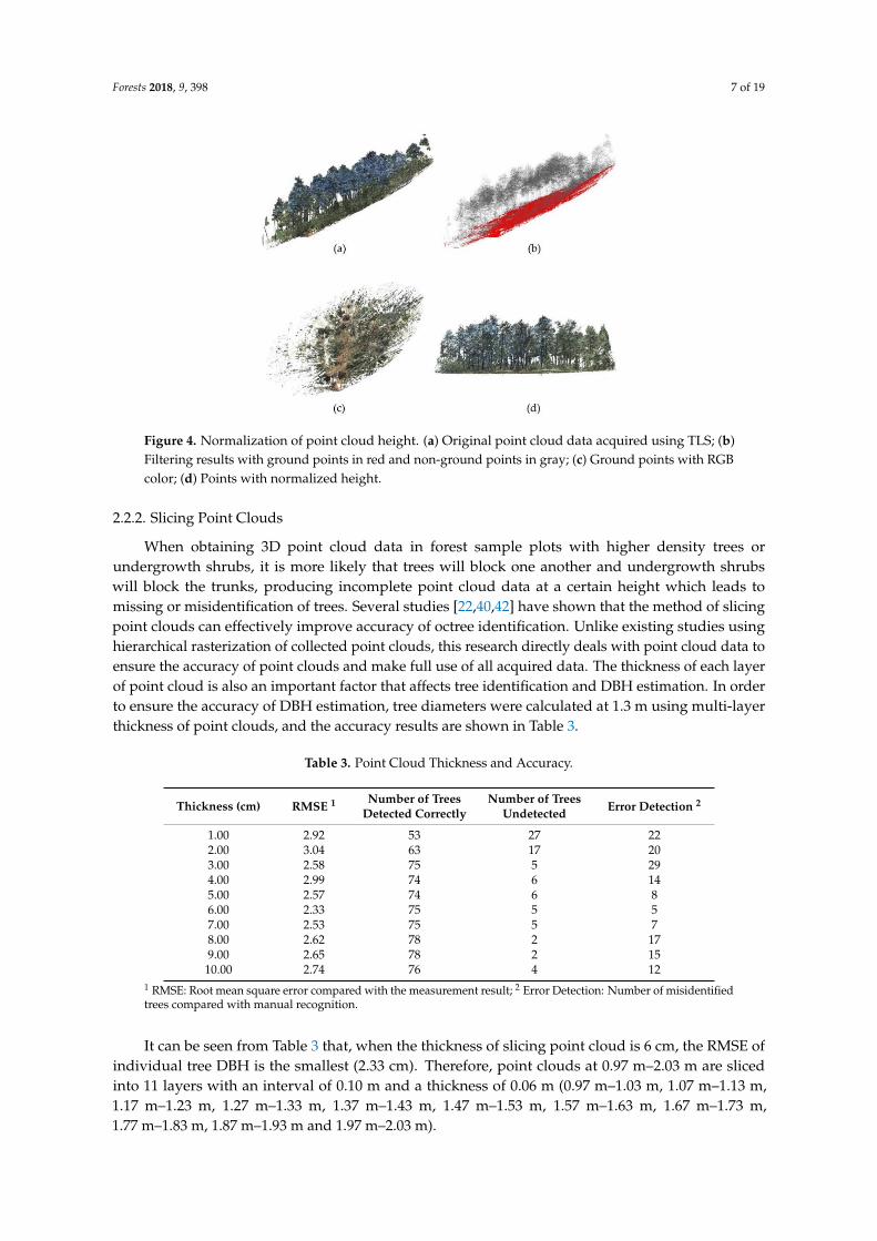
2.2.2. Slicing Point Clouds

When obtaining 3D point cloud data in forest sample plots with higher density trees or

undergrowth shrubs, it is more likely that trees will block one another and undergrowth shrubs will

block the trunks, producing incomplete point cloud data at a certain height which leads to missing

or misidentification of trees. Several studies [22,40,42] have shown that the method of slicing point

clouds can effectively improve accuracy of octree identification. Unlike existing studies using

hierarchical rasterization of collected point clouds, this research directly deals with point cloud data

to ensure the accuracy of point clouds and make full use of all acquired data. The thickness of each

layer of point cloud is also an important factor that affects tree identification and DBH estimation. In

order to ensure the accuracy of DBH estimation, tree diameters were calculated at 1.3 m using multi-

layer thickness of point clouds, and the accuracy results are shown in Table 3.

Table 3. Point Cloud Thickness and Accuracy.

Thickness

(cm) RMSE 1

Number of Trees

Detected Correctly

Number of Trees

Undetected

Error

Detection 2

1.00 2.92 53 27 22

2.00 3.04 63 17 20

3.00 2.58 75 5 29

4.00 2.99 74 6 14

5.00 2.57 74 6 8

6.00 2.33 75 5 5

7.00 2.53 75 5 7

8.00 2.62 78 2 17

9.00 2.65 78 2 15

10.00 2.74 76 4 12 1 RMSE: Root mean square error compared with the measurement result; 2 Error Detection: Number

of misidentified trees compared with manual recognition.

It can be seen from Table 3 that, when the thickness of slicing point cloud is 6 cm, the RMSE of

individual tree DBH is the smallest (2.33 cm). Therefore, point clouds at 0.97 m–2.03 m are sliced into

11 layers with an interval of 0.10 m and a thickness of 0.06 m (0.97 m–1.03 m, 1.07 m–1.13 m, 1.17 m–

Figure 4. Normalization of point cloud height. (a) Original point cloud data acquired using TLS; (b)Filtering results with ground points in red and non-ground points in gray; (c) Ground points with RGBcolor; (d) Points with normalized height.

2.2.2. Slicing Point Clouds

When obtaining 3D point cloud data in forest sample plots with higher density trees orundergrowth shrubs, it is more likely that trees will block one another and undergrowth shrubswill block the trunks, producing incomplete point cloud data at a certain height which leads tomissing or misidentification of trees. Several studies [22,40,42] have shown that the method of slicingpoint clouds can effectively improve accuracy of octree identification. Unlike existing studies usinghierarchical rasterization of collected point clouds, this research directly deals with point cloud data toensure the accuracy of point clouds and make full use of all acquired data. The thickness of each layerof point cloud is also an important factor that affects tree identification and DBH estimation. In orderto ensure the accuracy of DBH estimation, tree diameters were calculated at 1.3 m using multi-layerthickness of point clouds, and the accuracy results are shown in Table 3.

Table 3. Point Cloud Thickness and Accuracy.

Thickness (cm) RMSE 1 Number of TreesDetected Correctly

Number of TreesUndetected Error Detection 2

1.00 2.92 53 27 222.00 3.04 63 17 203.00 2.58 75 5 294.00 2.99 74 6 145.00 2.57 74 6 86.00 2.33 75 5 57.00 2.53 75 5 78.00 2.62 78 2 179.00 2.65 78 2 15

10.00 2.74 76 4 121 RMSE: Root mean square error compared with the measurement result; 2 Error Detection: Number of misidentifiedtrees compared with manual recognition.

It can be seen from Table 3 that, when the thickness of slicing point cloud is 6 cm, the RMSE ofindividual tree DBH is the smallest (2.33 cm). Therefore, point clouds at 0.97 m–2.03 m are slicedinto 11 layers with an interval of 0.10 m and a thickness of 0.06 m (0.97 m–1.03 m, 1.07 m–1.13 m,1.17 m–1.23 m, 1.27 m–1.33 m, 1.37 m–1.43 m, 1.47 m–1.53 m, 1.57 m–1.63 m, 1.67 m–1.73 m,1.77 m–1.83 m, 1.87 m–1.93 m and 1.97 m–2.03 m).

Forests 2018, 9, 398 8 of 19

2.2.3. Octree Segmentation and Connected Component Labeling

In order to reduce redundancy and improve processing efficiency and accuracy, octreesegmentation and connected component labeling are combined to segment the point clouds beforetrunks are identified.

The method of connected component labeling [54] is usually used to detect connected areas ofbinary images in the field of computer vision. It can be used for processing color images and higherdimensional data as well. Different from the image data, point cloud data is composed of a largenumber of independent, discrete points with spatial coordinates. Therefore, the method of octreesegmentation is used to obtain voxelization data of the hierarchical point cloud. Voxelization is aprocessing of point cloud segmentation based on octree. First, a closed minimal cube is determined asa root node or a zero-level node, and then the root node is subdivided into eight voxels recursively.Non-empty voxels continue to be divided until they are divided into the remaining thresholds or theminimum pixel size criteria are reached [55].

As shown in Figure 5, the raw point cloud contains a large number of useless points (shrubs,weeds, etc.). With the increasing depth of octree (Figure 5b–h), the points are divided into relativelyindependent spaces. When the octree level = 10, trunks, shrubs and weeds show better separability.By further increasing the depth of the octree (Octree level = 11 or Octree level = 12), the originalseparability between the trees is maintained, but the amount of data has increased substantially.Therefore, this study uses the octree segmentation method with octree level = 10 to voxelize each layerof cloud data of trunks. Based on voxelization of points, we use the method of connected componentlabeling to get point cloud voxels connected and complete the segmentation of tree stem form stratifiedpoint clouds. The segmentation results are shown in Figure 5i.

Forests 2018, 9, x FOR PEER REVIEW 8 of 19

1.23 m, 1.27 m–1.33 m, 1.37 m–1.43 m, 1.47 m–1.53 m, 1.57 m–1.63 m, 1.67 m–1.73 m, 1.77 m–1.83 m,

1.87 m–1.93 m and 1.97 m–2.03 m).

2.2.3. Octree Segmentation and Connected Component Labeling

In order to reduce redundancy and improve processing efficiency and accuracy, octree

segmentation and connected component labeling are combined to segment the point clouds before

trunks are identified.

The method of connected component labeling [54] is usually used to detect connected areas of

binary images in the field of computer vision. It can be used for processing color images and higher

dimensional data as well. Different from the image data, point cloud data is composed of a large

number of independent, discrete points with spatial coordinates. Therefore, the method of octree

segmentation is used to obtain voxelization data of the hierarchical point cloud. Voxelization is a

processing of point cloud segmentation based on octree. First, a closed minimal cube is determined

as a root node or a zero-level node, and then the root node is subdivided into eight voxels recursively.

Non-empty voxels continue to be divided until they are divided into the remaining thresholds or the

minimum pixel size criteria are reached [55].

As shown in Figure 5, the raw point cloud contains a large number of useless points (shrubs,

weeds, etc.). With the increasing depth of octree (Figure 5b–h), the points are divided into relatively

independent spaces. When the octree level = 10, trunks, shrubs and weeds show better separability.

By further increasing the depth of the octree (Octree level = 11 or Octree level = 12), the original

separability between the trees is maintained, but the amount of data has increased substantially.

Therefore, this study uses the octree segmentation method with octree level = 10 to voxelize each

layer of cloud data of trunks. Based on voxelization of points, we use the method of connected

component labeling to get point cloud voxels connected and complete the segmentation of tree stem

form stratified point clouds. The segmentation results are shown in Figure 5i.

Figure 5. Processing of octree segmentation and connected component labeling (top view). (a) Raw

point cloud with shrubs and weeds; (b–h) With the increasing depth of octree, the points are divided

into independent spaces relatively; (i) The point cloud is divided into different parts (represented by

Figure 5. Processing of octree segmentation and connected component labeling (top view). (a) Rawpoint cloud with shrubs and weeds; (b–h) With the increasing depth of octree, the points are dividedinto independent spaces relatively; (i) The point cloud is divided into different parts (represented bydifferent colors), and randomly taking points within a single area can effectively reduce the invalid loop.

Forests 2018, 9, 398 9 of 19

2.2.4. Random Hough Transform and DBH Extraction

The detailed process of extracting DBH using random Hough transform is shown in Figure 6.For sliced point cloud data, the RHT method is used to sequentially perform circular detection frommultiple sub-regions in each layer respectively until extraction of all sliced point cloud is completed.The process of extracting each sub-partition (point cloud set P) of each layer is as follows:

(1) First, the point set P is projected onto the X–Y plane in the direction of Z-axis to form a 2-Dpoint cloud set P′ (Figure 6f). Defining the Hough space M (m, n, r) is carried out, where m isthe number of grids with 0.01 m intervals for point cloud set P’ in the direction of X-axis, n isthe number of grids with 0.01 m intervals for P′ in the direction of Y-axis, and r is the radiusstored in millimeters (Figure 6g, the gray grid under points). Three points p1(x1, y1), p2(x2, y2),p3(x3, y3) that are non-collinear and where the distance between any two points is greater than0.02 m are selected from the point cloud set P’ randomly. The condition of three non-collinearpoints p1(x1, y1), p2(x2, y2), p3(x3, y3) can be expressed as:∣∣∣∣∣∣∣

x− x1 y− y1 z− z1

x2 − x1 y2 − y1 z2 − z1

x3 − x1 y3 − y1 z3 − z1

∣∣∣∣∣∣∣ = 0 (1)

The distance conditions between the points are:√(x1 − x2)

2 + (y1 − y2)2 > 0.02√

(x1 − x3)2 + (y1 − y3)

2 > 0.02√(x2 − x3)

2 + (y2 − y3)2 > 0.02

(2)

Then, these 3 points can form a circle C1, with the center point O1 (a1, b1) (Figure 6g) and theradius r1 of the circle can be obtained. According to our field survey results, if r1 > 0.7 or r1 < 0.03(trees with DBH larger than 1.40 m or less than 0.06 m are not extracted), a new set of three pointsshould be selected for calculating the radius ri until ri satisfies 0.03 ≤ ri ≤0.7. The correspondingHough parameter space is voted in as M(ai,bi,ri) = M(ai,bi,ri) + 1.

(2) This method is repeatedly performed on the remaining point clouds until the elements in P′ aredepleted, so that the final M is obtained. If the difference between the radii of two concentriccircles in M is less than 0.01 m, the circles are considered to be the same circle, the average radiusof all concentric circles is used as the final radius, and the final voting result is the sum of allcircles that meet the conditions. Formula (3) expresses the voting result in M:

M(ai, bi, ri)

max(M)> ε (3)

where, ε is the threshold value of a circle detected for sliced point cloud of trees. Many tests inthe study show that the accuracy of DBH extraction is high when ε = 0.80. The next conditionneeding to be tested is the relative position between any point (xi,yi) in point cloud P’ and thecircle Ci (ai,bi,ri) satisfying the voting result in M:√

(xi − ai)2 + (yi − bi)

2 < 0.7× ri (4)

Equation (4) indicates that there are points inside the identified trunk, which are inconsistentwith the actual results and should be excluded from the circle that satisfies the voting result.

(3) Using this method, all layers of point clouds are extracted, and the trunk position and the trunksection radius of each layer of trees are obtained. If the position of tree trunk is detected in fouror more layers, it is assumed that there is a tree at this position, and the single-wood position is

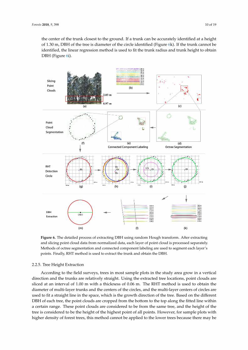
Forests 2018, 9, 398 10 of 19

the center of the trunk closest to the ground. If a trunk can be accurately identified at a heightof 1.30 m, DBH of the tree is diameter of the circle identified (Figure 6k). If the trunk cannot beidentified, the linear regression method is used to fit the trunk radius and trunk height to obtainDBH (Figure 6i).

Forests 2018, 9, x FOR PEER REVIEW 10 of 19

identified, the linear regression method is used to fit the trunk radius and trunk height to obtain

DBH (Figure 6i).

Figure 6. The detailed process of extracting DBH using random Hough transform. After extracting

and slicing point cloud data from normalized data, each layer of point cloud is processed separately.

Methods of octree segmentation and connected component labeling are used to segment each layer’s

points. Finally, RHT method is used to extract the trunk and obtain the DBH.

2.2.5. Tree Height Extraction

According to the field surveys, trees in most sample plots in the study area grow in a vertical

direction and the trunks are relatively straight. Using the extracted tree locations, point clouds are

sliced at an interval of 1.00 m with a thickness of 0.06 m. The RHT method is used to obtain the

diameter of multi-layer trunks and the centers of the circles, and the multi-layer centers of circles are

used to fit a straight line in the space, which is the growth direction of the tree. Based on the different

DBH of each tree, the point clouds are cropped from the bottom to the top along the fitted line within

a certain range. These point clouds are considered to be from the same tree, and the height of the tree

is considered to be the height of the highest point of all points. However, for sample plots with higher

density of forest trees, this method cannot be applied to the lower trees because there may be point

clouds of other trees along the growth direction of the trunk, as shown in Figure 7a. To handle such

situations, Liu et al. [22] adopted a method of vertical detection along the growth direction of the

trunk to calculate the tree height of the lower tree by counting the changes in the voxel of the point

cloud. However, the method can only reflect the change of the number of point clouds in the direction

Figure 6. The detailed process of extracting DBH using random Hough transform. After extractingand slicing point cloud data from normalized data, each layer of point cloud is processed separately.Methods of octree segmentation and connected component labeling are used to segment each layer’spoints. Finally, RHT method is used to extract the trunk and obtain the DBH.

2.2.5. Tree Height Extraction

According to the field surveys, trees in most sample plots in the study area grow in a verticaldirection and the trunks are relatively straight. Using the extracted tree locations, point clouds aresliced at an interval of 1.00 m with a thickness of 0.06 m. The RHT method is used to obtain thediameter of multi-layer trunks and the centers of the circles, and the multi-layer centers of circles areused to fit a straight line in the space, which is the growth direction of the tree. Based on the differentDBH of each tree, the point clouds are cropped from the bottom to the top along the fitted line withina certain range. These point clouds are considered to be from the same tree, and the height of thetree is considered to be the height of the highest point of all points. However, for sample plots withhigher density of forest trees, this method cannot be applied to the lower trees because there may be

Forests 2018, 9, 398 11 of 19

point clouds of other trees along the growth direction of the trunk, as shown in Figure 7a. To handlesuch situations, Liu et al. [22] adopted a method of vertical detection along the growth direction ofthe trunk to calculate the tree height of the lower tree by counting the changes in the voxel of thepoint cloud. However, the method can only reflect the change of the number of point clouds in thedirection of Z-axis, and cannot accurately stratify the different levels of trees. In order to detect theattributions of the tree point cloud effectively, extracted tree points (Figure 7b) are segmented usingthe CCL method based on the octree segmentation described previously. The segmentation result isshown in Figure 7c. It can be seen from Figure 7c that the algorithm separates points of the low treeand points of high-level tree accurately, and the height of the low tree can be obtained from the highestz value of the segmented tree.

Forests 2018, 9, x FOR PEER REVIEW 11 of 19

of Z-axis, and cannot accurately stratify the different levels of trees. In order to detect the attributions

of the tree point cloud effectively, extracted tree points (Figure 7b) are segmented using the CCL

method based on the octree segmentation described previously. The segmentation result is shown in

Figure 7c. It can be seen from Figure 7c that the algorithm separates points of the low tree and points

of high-level tree accurately, and the height of the low tree can be obtained from the highest z value

of the segmented tree.

Figure 7. Height extraction of trees in a natural forest. (a) Mixture of trees with different heights; (b)

The height of the highest point of a point cloud may not represent tree height; (c) Segmented tree

points.

3. Results and Discussion

3.1. Analysis of the Influence of Forest Density on Scanning Range and Accuracy

Forest point clouds collected by TLS are often affected by mutual shelter between trees. Mutual

obstruction between trunks results in lower accuracy in tree segmentation and DBH extraction, while

mutual shelter between canopies leads to lower accuracy of tree height extraction. From Table 1, it

can be seen that the Leica P40 can obtain a large range of high-precision 3D data. However, due to

the shelter between trees, the extent of scanning is limited, and the density of trees in forest limits the

size of forest sample plots. In order to ensure the accuracy of tree height and DBH extraction, three

typical sample plots of Pinus yunnanensis (plot numbers 20170726012, 20160831017 and 20160824002)

are selected to analyze the accuracy of the same tree species with different forest density (Table 4).

According to the result of that, we can determine a range of sample plots suitable.

It can be seen from Figure 8 and Table 4 that topography and forest density affect the scanning

range and scanning accuracy of the terrestrial laser scanner.

(1) The scanning range of high-density young forest sample plots is seriously affected by the mutual

obstruction between trees. Trees can be identified more accurately (99/106) within a range of 15

m centered on the central station, but there are a small number of missing trees (7 trees) due to

mutual shelter between trees within the forest sample plot (5 m–10 m). The identification

accuracy of trees near the edge of the young sample plot (distance from the center of the sample

plot > 15 m) is low, and there are a large number of missed trees (35). The DBH and extraction

accuracy of tree height of the entire sample plot is relatively high (mean RMSE of DBH is 1.03

cm, and mean RMSE of the tree height is 0.51 m). The maximum error is also located near the

edge of the sample plot.

(2) The scanning range of the medium–density plot is mainly affected by the topography and low

bushes under the forest canopy. In areas with low tree density and relatively flat terrain, a larger

range of scanning areas can be obtained and the accuracy of tree identification and height/DBH

extraction are higher as well. For the sample plot of NO. 20160831017, within the range of 20 m

Figure 7. Height extraction of trees in a natural forest. (a) Mixture of trees with different heights; (b)The height of the highest point of a point cloud may not represent tree height; (c) Segmented tree points.

3. Results and Discussion

3.1. Analysis of the Influence of Forest Density on Scanning Range and Accuracy

Forest point clouds collected by TLS are often affected by mutual shelter between trees. Mutualobstruction between trunks results in lower accuracy in tree segmentation and DBH extraction, whilemutual shelter between canopies leads to lower accuracy of tree height extraction. From Table 1, it canbe seen that the Leica P40 can obtain a large range of high-precision 3D data. However, due to theshelter between trees, the extent of scanning is limited, and the density of trees in forest limits thesize of forest sample plots. In order to ensure the accuracy of tree height and DBH extraction, threetypical sample plots of Pinus yunnanensis (plot numbers 20170726012, 20160831017 and 20160824002)are selected to analyze the accuracy of the same tree species with different forest density (Table 4).According to the result of that, we can determine a range of sample plots suitable.

It can be seen from Figure 8 and Table 4 that topography and forest density affect the scanningrange and scanning accuracy of the terrestrial laser scanner.

(1) The scanning range of high-density young forest sample plots is seriously affected by the mutualobstruction between trees. Trees can be identified more accurately (99/106) within a range of15 m centered on the central station, but there are a small number of missing trees (7 trees) dueto mutual shelter between trees within the forest sample plot (5 m–10 m). The identificationaccuracy of trees near the edge of the young sample plot (distance from the center of the sampleplot > 15 m) is low, and there are a large number of missed trees (35). The DBH and extractionaccuracy of tree height of the entire sample plot is relatively high (mean RMSE of DBH is 1.03 cm,

Forests 2018, 9, 398 12 of 19

and mean RMSE of the tree height is 0.51 m). The maximum error is also located near the edge ofthe sample plot.

(2) The scanning range of the medium–density plot is mainly affected by the topography and lowbushes under the forest canopy. In areas with low tree density and relatively flat terrain, a largerrange of scanning areas can be obtained and the accuracy of tree identification and height/DBHextraction are higher as well. For the sample plot of NO. 20160831017, within the range of 20 mfrom the center of the sample plot, 64 out of 66 trees are identified, with an RMSE of 1.28 cm forDBH, and an RMSE of 0.57 m for tree height. When the distance from the tree to the center of thesample plot exceeds 20 m, the tree recognition accuracy decreases slightly. The tree height andDBH extraction accuracy also slightly decreases with the increase of the distance from the tree tothe center of the sample plot.

(3) Low–density mature forests have a relatively complete vertical structure of individual trees.The growth space under the forest canopy is sufficient for the growth of low shrubs. It can beseen from the point clouds (Plot 20160824002) that a large number of shrub points are includedin the point cloud near the ground. Meanwhile, the effective range of sample plots obtainedby multi–station scanning is limited due to terrain influences. It can be seen from Table 4 thatextraction results obtained within the range of 20 m is better than those beyond the range: The treedetection rate is high (36/40), with an RMSE of 1.24 cm for DBH, and an RMSE of 0.46 m for treeheight. When the distance from the tree to the TLS scanner is more than 20 m, the accuracy oftree detection is slightly reduced (40/51) due to the longer distance and the influence of shrubsaround the station.

Forests 2018, 9, x FOR PEER REVIEW 12 of 19

from the center of the sample plot, 64 out of 66 trees are identified, with an RMSE of 1.28 cm for

DBH, and an RMSE of 0.57 m for tree height. When the distance from the tree to the center of

the sample plot exceeds 20 m, the tree recognition accuracy decreases slightly. The tree height

and DBH extraction accuracy also slightly decreases with the increase of the distance from the

tree to the center of the sample plot.

(3) Low–density mature forests have a relatively complete vertical structure of individual trees. The

growth space under the forest canopy is sufficient for the growth of low shrubs. It can be seen

from the point clouds (Plot 20160824002) that a large number of shrub points are included in the

point cloud near the ground. Meanwhile, the effective range of sample plots obtained by multi–

station scanning is limited due to terrain influences. It can be seen from Table 4 that extraction

results obtained within the range of 20 m is better than those beyond the range: The tree

detection rate is high (36/40), with an RMSE of 1.24 cm for DBH, and an RMSE of 0.46 m for tree

height. When the distance from the tree to the TLS scanner is more than 20 m, the accuracy of

tree detection is slightly reduced (40/51) due to the longer distance and the influence of shrubs

around the station.

Figure 8. Results of trunk extraction in different density plots of Pinus yunnanensis.

Table 4. Effects of Forest Density and Distance on Scanning Range and Accuracy.

Plot # Stand Age Mean

DBH

Mean

T.H. 1

<5 m 5 m–10 m

RMSE Trees

Num.

ER

Trees 2

RMSE Trees

Num.

ER

Trees DBH T.H. DBH T.H.

20170726012 Young 11.30 8.2 0.91 0.41 13 0 1.09 0.44 43 7

20160831017 Middle-age 24.70 15.2 1.27 0.54 2 0 1.20 0.89 18 0

20160824002 Mature 28.40 18.0 0.68 0.59 2 0 1.64 0.46 6 0

10 m–15 m 15–20 m >20 m

RMSE Trees

Num

ER

Trees

RMSE Trees

Num.

ER

Trees

RMSE Trees

Num. ER Trees

DBH T.H. DBH T.H. DBH T.H.

0.81 0.57 43 0 1.30 0.60 12 35 – – □ –

1.28 0.56 18 1 1.36 0.30 26 1 1.33 0.78 218 30

1.64 0.52 10 2 1.00 0.17 18 2 1.43 0.84 40 11

1 T.H.: Tree Height; 2 ER Trees: Error trees, misidentified trees.

Figure 8. Results of trunk extraction in different density plots of Pinus yunnanensis.

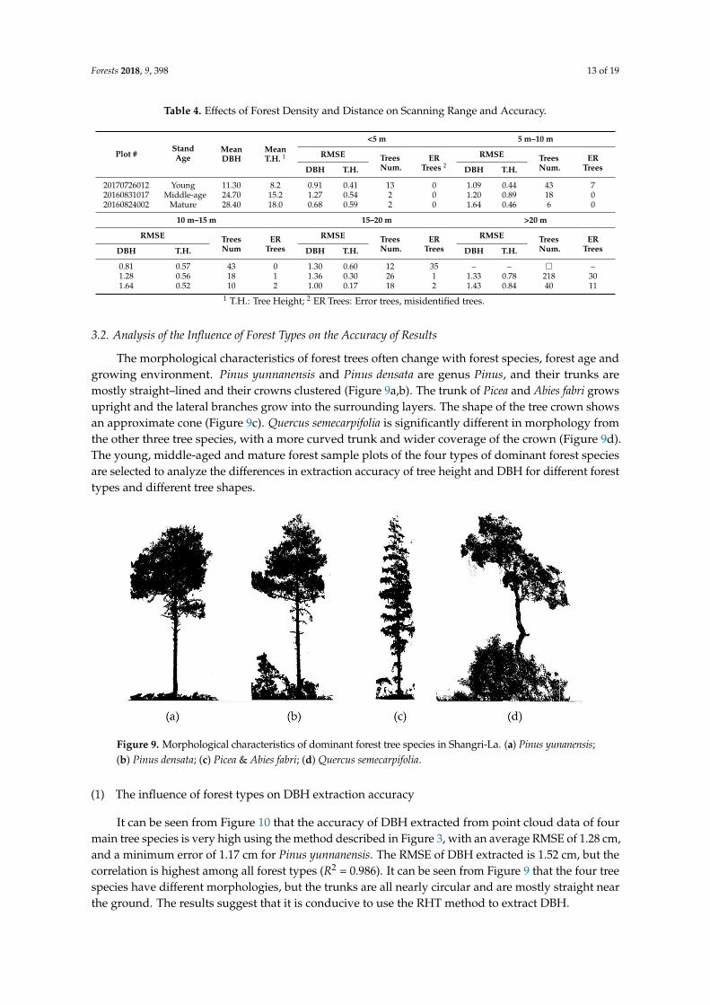
Forests 2018, 9, 398 13 of 19

Table 4. Effects of Forest Density and Distance on Scanning Range and Accuracy.

Plot #StandAge

MeanDBH

MeanT.H. 1

<5 m 5 m–10 m

RMSE TreesNum.

ERTrees 2

RMSE TreesNum.

ERTreesDBH T.H. DBH T.H.

20170726012 Young 11.30 8.2 0.91 0.41 13 0 1.09 0.44 43 720160831017 Middle-age 24.70 15.2 1.27 0.54 2 0 1.20 0.89 18 020160824002 Mature 28.40 18.0 0.68 0.59 2 0 1.64 0.46 6 0

10 m–15 m 15–20 m >20 m

RMSE TreesNum

ERTrees

RMSE TreesNum.

ERTrees

RMSE TreesNum.

ERTreesDBH T.H. DBH T.H. DBH T.H.

0.81 0.57 43 0 1.30 0.60 12 35 – – � –1.28 0.56 18 1 1.36 0.30 26 1 1.33 0.78 218 301.64 0.52 10 2 1.00 0.17 18 2 1.43 0.84 40 11

1 T.H.: Tree Height; 2 ER Trees: Error trees, misidentified trees.

3.2. Analysis of the Influence of Forest Types on the Accuracy of Results

The morphological characteristics of forest trees often change with forest species, forest age andgrowing environment. Pinus yunnanensis and Pinus densata are genus Pinus, and their trunks aremostly straight–lined and their crowns clustered (Figure 9a,b). The trunk of Picea and Abies fabri growsupright and the lateral branches grow into the surrounding layers. The shape of the tree crown showsan approximate cone (Figure 9c). Quercus semecarpifolia is significantly different in morphology fromthe other three tree species, with a more curved trunk and wider coverage of the crown (Figure 9d).The young, middle-aged and mature forest sample plots of the four types of dominant forest speciesare selected to analyze the differences in extraction accuracy of tree height and DBH for different foresttypes and different tree shapes.

Forests 2018, 9, x FOR PEER REVIEW 13 of 19

3.2. Analysis of the Influence of Forest Types on the Accuracy of Results

The morphological characteristics of forest trees often change with forest species, forest age and

growing environment. Pinus yunnanensis and Pinus densata are genus Pinus, and their trunks are

mostly straight–lined and their crowns clustered (Figure 9a,b). The trunk of Picea and Abies fabri

grows upright and the lateral branches grow into the surrounding layers. The shape of the tree crown

shows an approximate cone (Figure 9c). Quercus semecarpifolia is significantly different in morphology

from the other three tree species, with a more curved trunk and wider coverage of the crown (Figure

9d). The young, middle-aged and mature forest sample plots of the four types of dominant forest

species are selected to analyze the differences in extraction accuracy of tree height and DBH for

different forest types and different tree shapes.

Figure 9. Morphological characteristics of dominant forest tree species in Shangri-La. (a) Pinus

yunanensis; (b) Pinus densata; (c) Picea & Abies fabri; (d) Quercus semecarpifolia.

(1) The influence of forest types on DBH extraction accuracy

It can be seen from Figure 10 that the accuracy of DBH extracted from point cloud data of four

main tree species is very high using the method described in Figure 3, with an average RMSE of 1.28

cm, and a minimum error of 1.17 cm for Pinus yunnanensis. The RMSE of DBH extracted is 1.52 cm,

but the correlation is highest among all forest types (R2 = 0.986). It can be seen from Figure 9 that the

four tree species have different morphologies, but the trunks are all nearly circular and are mostly

straight near the ground. The results suggest that it is conducive to use the RHT method to extract

DBH.

Figure 9. Morphological characteristics of dominant forest tree species in Shangri-La. (a) Pinus yunanensis;(b) Pinus densata; (c) Picea & Abies fabri; (d) Quercus semecarpifolia.

(1) The influence of forest types on DBH extraction accuracy

It can be seen from Figure 10 that the accuracy of DBH extracted from point cloud data of fourmain tree species is very high using the method described in Figure 3, with an average RMSE of 1.28 cm,and a minimum error of 1.17 cm for Pinus yunnanensis. The RMSE of DBH extracted is 1.52 cm, but thecorrelation is highest among all forest types (R2 = 0.986). It can be seen from Figure 9 that the four treespecies have different morphologies, but the trunks are all nearly circular and are mostly straight nearthe ground. The results suggest that it is conducive to use the RHT method to extract DBH.

Forests 2018, 9, 398 14 of 19Forests 2018, 9, x FOR PEER REVIEW 14 of 19

Figure 10. Accuracy analysis of four dominant forest species in Shangri-La. (a) Pinus yunanensis; (b)

Pinus densata; (c) Picea & Abies fabri; (d) Quercus semecarpifolia.

(2) The effect of tree species on tree height extraction accuracy

Several studies [38,56,57] have shown that the extraction of forest trees by TLS cannot obtain the

point cloud information at the top of the canopy due to the mutual occlusion between canopies, which

Figure 10. Accuracy analysis of four dominant forest species in Shangri-La. (a,b) Pinus yunanensis;(c,d) Pinus densata; (e,f) Picea & Abies fabri; (g,h) Quercus semecarpifolia.

(2) The effect of tree species on tree height extraction accuracy

Several studies [38,56,57] have shown that the extraction of forest trees by TLS cannot obtainthe point cloud information at the top of the canopy due to the mutual occlusion between canopies,which leads to an underestimation of tree height. The forest in the study area is mainly coniferous with

Forests 2018, 9, 398 15 of 19

some broad-leaved trees. Compared with broadleaf forests, coniferous forest canopy has some voids,and relatively accurate tree heights can be obtained in a certain range when the stations are properlyarranged. It can be seen from Figure 10 that the largest underestimation of tree height is from Picea& Abies fabri (RMSE = 1.28 m), followed by Quercus semecarpifolia, Pinus densata and Pinus yunanensis.The mean RMSE of 4 species is 0.95 m, and all of them showed good correlation.

3.3. Accuracy Analysis of Results in Forest Sample Plots

Major elements of forest surveys include tree diameter, height, coverage, and density, amongwhich the tree height and diameter are the most important ones. Mean DBH is the diametercorresponding to the average basal area of dominant tree species, which is a basic index reflectingthe forest roughness. The methods of calculating mean DBH include the arithmetic mean method,quadratic mean method, volume mean method, mode method, and median method. At present,the method of quadratic mean is commonly used in forest surveys:

D =

√∑ d2

in

(5)

where, D is the mean DBH, di is the DBH of tree i, and n is the total number of trees in forestsample plots.

The mean stand height is an important indicator that reflects the height level of stands, and it isan important tree parameter in forest surveys. For the measurement of arborous forest, it should bedetermined by selecting 3 to 5 average sample trees among the main forest layer dominant tree speciesaccording to the average DBH, and the average tree height should be calculated using the arithmeticmean method.

In this paper, the mean DBH and mean stand height are calculated by using the methods above,and compared with the measured data in sample plots for accuracy assessment. It can be seen fromFigure 11 that the mean DBH and mean tree height extracted by the RHT method combined withoctree segmentation have strong correlations (correlation of DBH is R2 = 0.957, correlation of treeheight is R2 = 0.905) with the measured data. The mean RMSE of the extracting method is 1.96 cm.The smaller the mean DBH, the higher the extraction accuracy. With the increase of the mean DBHin plots, the errors tend to increase slightly. The RMSE of the extracted mean stand height is 1.40 m.Because the canopy obscures the point cloud, results of tree height extracted by TLS data are slightlylower than the actual tree height in forest sample plots with higher average tree heights.

Forests 2018, 9, x FOR PEER REVIEW 15 of 19

leads to an underestimation of tree height. The forest in the study area is mainly coniferous with some

broad-leaved trees. Compared with broadleaf forests, coniferous forest canopy has some voids, and

relatively accurate tree heights can be obtained in a certain range when the stations are properly

arranged. It can be seen from Figure 10 that the largest underestimation of tree height is from Picea &

Abies fabri (RMSE = 1.28 m), followed by Quercus semecarpifolia, Pinus densata and Pinus yunanensis.

The mean RMSE of 4 species is 0.95 m, and all of them showed good correlation.

3.3. Accuracy Analysis of Results in Forest Sample Plots

Major elements of forest surveys include tree diameter, height, coverage, and density, among

which the tree height and diameter are the most important ones. Mean DBH is the diameter

corresponding to the average basal area of dominant tree species, which is a basic index reflecting

the forest roughness. The methods of calculating mean DBH include the arithmetic mean method,

quadratic mean method, volume mean method, mode method, and median method. At present, the

method of quadratic mean is commonly used in forest surveys:

�� = √∑𝑑𝑖

2

𝑛 (5)

where, D is the mean DBH, di is the DBH of tree i, and n is the total number of trees in forest sample

plots.

The mean stand height is an important indicator that reflects the height level of stands, and it is

an important tree parameter in forest surveys. For the measurement of arborous forest, it should be

determined by selecting 3 to 5 average sample trees among the main forest layer dominant tree

species according to the average DBH, and the average tree height should be calculated using the

arithmetic mean method.

In this paper, the mean DBH and mean stand height are calculated by using the methods above,

and compared with the measured data in sample plots for accuracy assessment. It can be seen from

Figure 11 that the mean DBH and mean tree height extracted by the RHT method combined with

octree segmentation have strong correlations (correlation of DBH is R2 = 0.957, correlation of tree

height is R2 = 0.905) with the measured data. The mean RMSE of the extracting method is 1.96 cm.

The smaller the mean DBH, the higher the extraction accuracy. With the increase of the mean DBH

in plots, the errors tend to increase slightly. The RMSE of the extracted mean stand height is 1.40 m.

Because the canopy obscures the point cloud, results of tree height extracted by TLS data are slightly

lower than the actual tree height in forest sample plots with higher average tree heights.

Figure 11. Accuracy analysis of DBH and tree height in forest sample plots.

4. Conclusions

Figure 11. Accuracy analysis of DBH and tree height in forest sample plots.

Forests 2018, 9, 398 16 of 19

4. Conclusions

The study focused on extracting tree height and DBH data of natural forest species at plot level inShangri-La, Northwest Yunnan, China. Combining methods of octree segmentation, CCL and RHTalgorithm, tree heights and DBH of natural forests at individual tree level and plot level were obtained.Topography, understory shrubs and tree density influence the TLS scanning range and accuracyof results. Because of different morphology of different tree species in Shangri-La, the accuracy oftree height and DBH extraction for different tree species is different using the method. In general,Pinus yunnanensis, Pinus densata and Picea & Abies fabria are coniferous forests, with vertical trunks andsimilar morphological structures and tree height extraction precision is high. Quercus semecarpifolia is abroad–leaved forest species, and its morphology is different from that of coniferous forest, leadingto relatively low extraction accuracy. In general, the methods used in the study have high accuracyfor the extraction of DBH and tree height for four dominant tree species in Shangri-La. The averageRMSE of DBH is 1.28 cm, and the average RMSE of tree height is 0.95 m. The results at forest sampleplot levels also show that the method can obtain the mean tree height and mean DBH accurately incomplex terrains. In the last few years, mobile/personal laser scanning and image-based techniqueshave become capable of providing similar 3D point cloud data, and have their own advantages,e.g., lower cost when using image-based techniques and high efficiency when using mobile/personallaser scanning. Further studies need to demonstrate the added value of using TLS, which mostprobably comes from the highly accurate tree attribute estimates.

Author Contributions: J.W., P.D. and G.L. conceived and designed the experiments; Y.C. performed theexperiments; Z.L. analyzed the data; and G.L. wrote the paper. All authors read and approved the final manuscript.

Funding: This research was funded by the National Natural Science Foundation of P.R. China grant number41271230 and 41561048.

Acknowledgments: Thanks to Cheng Wang of the Institute of Remote Sensing and Digital Earth, ChineseAcademy of Sciences for providing guidance in data collection and processing.

Conflicts of Interest: The authors declare no conflict of interest.

References

1. Wu, D.; Li, B.; Yang, A. Estimation of tree height and biomass based on long time series data of landsat.Eng. Surv. Mapp. 2017, 1–5. [CrossRef]

2. Lu, D. Aboveground biomass estimation using landsat TM data in the Brazilian amazon. Int. J. Remote Sens.2005, 26, 2509–2525. [CrossRef]

3. Liu, X.; Dan, Z.; Xing, Y. Study on Crown Diameter Extraction and Tree Height Inversion Based onHigh-resolution Images of UAV. Cent. South For. Invent. Plan. 2017, 36, 39–43. [CrossRef]

4. Dong, L. New Development of Forest Canopy Height Remote Sensing. Remote Sens. Technol. Appl. 2016, 31,833–845. [CrossRef]

5. Ozdemir, I.; Karnieli, A. Predicting forest structural parameters using the image texture derived fromworldview-2 multispectral imagery in a dryland forest, Israel. Int. J. Appl. Earth Obs. Geoinform. 2011, 13,701–710. [CrossRef]

6. Gibbs, H.K.; Brown, S.; Niles, J.O.; Foley, J.A. Monitoring and estimating tropical forest carbon stocks:Making redd a reality. Environ. Res. Lett. 2007, 2, 045023. [CrossRef]

7. Chopping, M.; Nolin, A.; Moisen, G.G.; Martonchik, J.V.; Bull, M. Forest canopy height from the multiangleimaging spectroradiometer (MISR) assessed with high resolution discrete return lidar. Remote Sens. Environ.2009, 113, 2172–2185. [CrossRef]

8. Rauste, Y. Multi-temporal jers sar data in boreal forest biomass mapping. Remote Sens. Environ. 2005, 97,263–275. [CrossRef]

9. Wang, Y. Estimation of Forest Volume Based on Multi-Source Remote Sensing Data; Beijing Forestry University:Beijing, China, 2015.

Forests 2018, 9, 398 17 of 19

10. Watanabe, M.; Motohka, T.; Thapa, R.B.; Shimada, M. Correlation between L-band SAR PolarimetricParameters and LiDAR Metrics over a Forested Area. In Proceedings of the 2015 IEEE InternationalGeoscience and Remote Sensing Symposium (IGARSS), Milan, Italy, 26–31 July 2015; pp. 1574–1577.[CrossRef]

11. Solberg, S.; Astrup, R.; Gobakken, T.; Næsset, E.; Weydahl, D.J. Estimating spruce and pine biomass withinterferometric X-band SAR. Remote Sens. Environ. 2010, 114, 2353–2360. [CrossRef]

12. Magnard, C.; Morsdorf, F.; Small, D.; Stilla, U.; Schaepman, M.E.; Meier, E. Single tree identification usingairborne multibaseline sar interferometry data. Remote Sens. Environ. 2016, 186, 567–580. [CrossRef]

13. Wu, Y.; Hong, W.; Wang, Y. The Current Status and Implications of Polarimetric SAR Interferometry.J. Electron. Inf. Technol. 2007, 29, 1258–1262.

14. Khati, U.; Kumar, S.; Agrawal, S.; Singh, J. Forest height estimation using space-borne polinsar dataset overtropical forests of India. ESA POLinSAR 2015, 4. [CrossRef]

15. Luo, H.; Chen, E.; Li, Z.; Cao, C. Forest above ground biomass estimation methodology based on polarizationcoherence tomography. J. Remote Sens. 2011, 15, 1138–1155. [CrossRef]

16. Schaedel, M.S.; Larson, A.J.; Affleck, D.L.; Belote, R.T.; Goodburn, J.M.; Wright, D.K.; Sutherland, E.K.Long-term precommercial thinning effects on larix occidentalis (western larch) tree and stand characteristics.Can. J. For. Res. 2017, 47, 861–874. [CrossRef]

17. Huang, K.; Pang, Y.; Shu, Q.; Fu, T. Aboveground forest biomass estimation using ICESat GLAS in Yunnan,China. J. Remote Sens. 2013, 17, 169–183. [CrossRef]

18. Man, Q.; Dong, P.; Guo, H.; Liu, G.; Shi, R. Light detection and ranging and hyperspectral data for estimationof forest biomass: A review. J. Appl. Remote Sens. 2014, 8, 081598. [CrossRef]

19. Xing, Y.; Wang, L. ICESat-GLAS Full Waveform-based Study on Forest Canopy Height Retrieval in SlopedArea—A Case Study of Forests in Changbai Mountains, Jilin. Geomat. Inf. Sci. Wuhan Univ. 2009, 34, 696–700.

20. Nie, S.; Wang, C.; Zeng, H.; Xi, X.; Xia, S. A revised terrain correction method for forest canopy heightestimation using icesat/glas data. ISPRS J. Photogramm. Remote Sens. 2015, 108, 183–190. [CrossRef]

21. Li, Z.; Liu, Q.; Pang, Y. Review on forest parameters inversion using LiDAR. J. Remote Sens. 2016, 20,1138–1150. [CrossRef]

22. Liu, L.; Pang, Y.; Li, Z. Individual Tree DBH and Height Estimation Using Terrestrial Laser Scanning (TLS) inA Subtropical Forest. Sci. Silvae Sin. 2016, 52, 26–37. [CrossRef]

23. Liang, X.; Kankare, V.; Hyyppä, J.; Wang, Y.; Kukko, A.; Haggrén, H.; Yu, X.; Kaartinen, H.; Jaakkola, A.;Guan, F. Terrestrial laser scanning in forest inventories. ISPRS J. Photogramm. Remote Sens. 2016, 115, 63–77.[CrossRef]

24. Nuttens, T.; De Wulf, A.; Bral, L.; De Wit, B.; Carlier, L.; De Ryck, M.; Stal, C.; Constales, D.; De Backer, H.High Resolution Terrestrial Laser Scanning for Tunnel Deformation Measurements. In Proceedings of the2010 FIG Congress, Sydney, Australia, 11–16 April 2010.

25. Fröhlich, C.; Mettenleiter, M. Terrestrial laser scanning—New perspectives in 3d surveying. Int. Arch.Photogramm. Remote Sens. Spat. Inf. Sci. 2004, 36, W2.

26. Telling, J.; Lyda, A.; Hartzell, P.; Glennie, C. Review of earth science research using terrestrial laser scanning.Earth Sci. Rev. 2017, 169, 35–68. [CrossRef]

27. Buckley, S.J.; Howell, J.; Enge, H.; Kurz, T. Terrestrial laser scanning in geology: Data acquisition, processingand accuracy considerations. J. Geol. Soc. 2008, 165, 625–638. [CrossRef]

28. Abellán, A.; Jaboyedoff, M.; Oppikofer, T.; Vilaplana, J. Detection of millimetric deformation using a terrestriallaser scanner: Experiment and application to a rockfall event. Nat. Hazards Earth Syst. Sci. 2009, 9, 365–372.[CrossRef]

29. Prokop, A.; Panholzer, H. Assessing the capability of terrestrial laser scanning for monitoring slow movinglandslides. Nat. Hazards Earth Syst. Sci. 2009, 9, 1921–1928. [CrossRef]

30. Olsen, M.J.; Cheung, K.F.; Yamazaki, Y.; Butcher, S.; Garlock, M.; Yim, S.; McGarity, S.; Robertson, I.;Burgos, L.; Young, Y.L. Damage assessment of the 2010 chile earthquake and tsunami using terrestrial laserscanning. Earthq. Spectra 2012, 28, S179–S197. [CrossRef]

31. Rosser, N.; Petley, D.; Lim, M.; Dunning, S.; Allison, R. Terrestrial laser scanning for monitoring the processof hard rock coastal cliff erosion. Q. J. Eng. Geol. Hydrogeol. 2005, 38, 363–375. [CrossRef]

Forests 2018, 9, 398 18 of 19

32. Vos, S.; Lindenbergh, R.; de Vries, S.; Aagaard, T.; Deigaard, R.; Fuhrman, D. Coastscan: Continuousmonitoring of coastal change using terrestrial laser scanning. In Proceedings of the Coastal Dynamics 2017,Helsingør, Denmark, 12–16 June 2017; Volume 233, pp. 1518–1528.

33. Kuhn, D.; Prüfer, S. Coastal cliff monitoring and analysis of mass wasting processes with the application ofterrestrial laser scanning: A case study of Rügen, Germany. Geomorphology 2014, 213, 153–165. [CrossRef]

34. Anderson, K.E.; Glenn, N.F.; Spaete, L.P.; Shinneman, D.J.; Pilliod, D.S.; Arkle, R.S.; McIlroy, S.K.;Derryberry, D.R. Methodological considerations of terrestrial laser scanning for vegetation monitoringin the sagebrush steppe. Environ. Monit. Assess. 2017, 189, 578. [CrossRef] [PubMed]

35. Pirotti, F.; Guarnieri, A.; Vettore, A. Ground filtering and vegetation mapping using multi-return terrestriallaser scanning. ISPRS J. Photogram. Remote Sens. 2013, 76, 56–63. [CrossRef]

36. Vaaja, M.; Hyyppä, J.; Kukko, A.; Kaartinen, H.; Hyyppä, H.; Alho, P. Mapping topography changes andelevation accuracies using a mobile laser scanner. Remote Sens. 2011, 3, 587–600. [CrossRef]

37. Srinivasan, S.; Popescu, S.C.; Eriksson, M.; Sheridan, R.D.; Ku, N.-W. Terrestrial laser scanning as an effectivetool to retrieve tree level height, crown width, and stem diameter. Remote Sens. 2015, 7, 1877–1896. [CrossRef]

38. Moskal, L.M.; Zheng, G. Retrieving forest inventory variables with terrestrial laser scanning (TLS) in urbanheterogeneous forest. Remote Sens. 2011, 4, 1–20. [CrossRef]

39. Thies, M.; Spiecker, H. Evaluation and future prospects of terrestrial laser scanning for standardized forestinventories. Forest 2004, 2, 1.

40. Li, D.; Pang, Y.; Yue, C.; Zhao, D.; Xue, G. Extraction of individual tree DBH and height based on terrestriallaser scanner data. J. Beijing For. Univ. 2012, 34, 79–86. [CrossRef]

41. Bienert, A.; Scheller, S.; Keane, E.; Mullooly, G.; Mohan, F. Application of terrestrial laser scannersfor the determination of forest inventory parameters. In Proceedings of the International Archives ofPhotogrammetry, Remote Sensing and Spatial Information Sciences, Dresden, Germany, 25–27 September2006; Volume 36.

42. Brolly, G.; Király, G. Algorithms for stem mapping by means of terrestrial laser scanning. Acta Silvaticaet Lignaria Hungarica 2009, 5, 119–130.

43. Shang, R.; Xi, X.; Wang, C.; Wang, X.; Luo, S. Retrieval of individual tree parameters using terrestrial laserscanning data. Sci. Surv. Mapp. 2015, 40, 78–81. [CrossRef]

44. Janowski, A. The circle object detection with the use of msplit estimation. E3S Web Conf. 2018, 26, 00014.[CrossRef]

45. Janowski, A.; Bobkowska, K.; Szulwic, J. 3D modelling of cylindrical-shaped objects from lidar data-anassessment based on theoretical modelling and experimental data. Metrol. Meas. Syst. 2018, 25. [CrossRef]

46. Bobkowska, K.; Szulwic, J.; Tysiac, P. Bus bays inventory using a terrestrial laser scanning system. MATECWeb Conf. 2017, 122, 04001. [CrossRef]

47. Cao, T.; Xiao, A.; Wu, L.; Mao, L. Automatic fracture detection based on terrestrial laser scanning data: A newmethod and case study. Comput. Geosci. 2017, 106, 209–216. [CrossRef]

48. Wezyk, P.; Koziol, K.; Glista, M.; Pierzchalski, M. Terrestrial laser scanning versus traditional forest inventoryfirst results from the polish forests. Tanpakushitsu Kakusan Koso Protein Nucleic Acid Enzyme 2007, 44, 325–337.

49. Cernava, J.; Tucek, J.; Koren, M.; Mokroš, M. Estimation of diameter at breast height from mobile laserscanning data collected under a heavy forest canopy. J. For. Sci. 2017, 63, 433–441.

50. Wezyk, P.; Koziol, K.; Glista, M.; Pierzchalski, M. Terrestrial Laser Scanning Versus Traditional ForestInventory: First Results from the Polish Forests. In Proceedings of the ISPRS Workshop on Laser Scanning,Espoo, Finland, 12–14 September 2007; pp. 12–14.

51. Olofsson, K.; Holmgren, J.; Olsson, H. Tree stem and height measurements using terrestrial laser scanningand the ransac algorithm. Remote Sens. 2014, 6, 4323–4344. [CrossRef]

52. Zhang, K.; Chen, S.-C.; Whitman, D.; Shyu, M.-L.; Yan, J.; Zhang, C. A progressive morphological filter forremoving nonground measurements from airborne lidar data. IEEE Trans. Geosci. Remote Sens. 2003, 41,872–882. [CrossRef]

53. Serra, J.; Vincent, L. An overview of morphological filtering. Circ. Syst. Signal Process. 1992, 11, 47–108.[CrossRef]

54. Dillencourt, M.B.; Samet, H.; Tamminen, M. A general approach to connected-component labeling forarbitrary image representations. J. ACM 1992, 39, 253–280. [CrossRef]

Forests 2018, 9, 398 19 of 19

55. Vo, A.-V.; Truong-Hong, L.; Laefer, D.F.; Bertolotto, M. Octree-based region growing for point cloudsegmentation. ISPRS J. Photogram. Remote Sens. 2015, 104, 88–100. [CrossRef]

56. Király, G.; Brolly, G. Tree height estimation methods for terrestrial laser scanning in a forest reserve. Int. Arch.Photogram. Remote Sens. Spat. Inf. Sci. 2007, 36, 211–215.

57. Kankare, V.; Holopainen, M.; Vastaranta, M.; Puttonen, E.; Yu, X.; Hyyppä, J.; Vaaja, M.; Hyyppä, H.; Alho, P.Individual tree biomass estimation using terrestrial laser scanning. ISPRS J. Photogram. Remote Sens. 2013, 75,64–75. [CrossRef]

© 2018 by the authors. Licensee MDPI, Basel, Switzerland. This article is an open accessarticle distributed under the terms and conditions of the Creative Commons Attribution(CC BY) license (http://creativecommons.org/licenses/by/4.0/).