Embed Size (px)
Citation preview

An Exact Solver for the Weston-Watkins SVM Subproblem
Yutong Wang 1 Clayton Scott 1 2
Abstract
Recent empirical evidence suggests that theWeston-Watkins support vector machine isamong the best performing multiclass exten-sions of the binary SVM. Current state-of-the-artsolvers repeatedly solve a particular subproblemapproximately using an iterative strategy. In thiswork, we propose an algorithm that solves thesubproblem exactly using a novel reparametriza-tion of the Weston-Watkins dual problem. Forlinear WW-SVMs, our solver shows significantspeed-up over the state-of-the-art solver when thenumber of classes is large. Our exact subproblemsolver also allows us to prove linear convergenceof the overall solver.
1. IntroductionSupport vector machines (SVMs) (Boser et al., 1992;Cortes & Vapnik, 1995) are a powerful class of algorithmsfor classification. In the large scale studies by Fernandez-Delgado et al. (2014) and by Klambauer et al. (2017),SVMs are shown to be among the best performing clas-sifers.
The original formulation of the SVM handles only binaryclassification. Subsequently, several variants of multiclassSVMs have been proposed (Lee et al., 2004; Crammer& Singer, 2001; Weston & Watkins, 1999). However, aspointed out by Dogan et al. (2016), no variant has beenconsidered canonical.
The empirical study of Dogan et al. (2016) compared nineprominent variants of multiclass SVMs and demonstratedthat the Weston-Watkins (WW) and Crammer-Singer (CS)SVMs performed the best with the WW-SVM holding aslight edge in terms of both efficiency and accuracy. This
1Department of Electrical Engineering and Computer Sci-ence, University of Michigan. 2Department of Statistics, Uni-versity of Michigan. Correspondence to: Yutong Wang <[email protected]>, Clayton Scott <[email protected]>.
Proceedings of the 38 th International Conference on MachineLearning, PMLR 139, 2021. Copyright 2021 by the author(s).
work focuses on the computational issues of solving theWW-SVM optimization efficiently.
SVMs are typically formulated as quadratic programs.State-of-the-art solvers such as LIBSVM (Chang & Lin,2011) and LIBLINEAR (Fan et al., 2008) apply block co-ordinate descent to the associated dual problem, which en-tails repeatedly solving many small subproblems. For thebinary case, these subproblems are easy to solve exactly.
The situation in the multiclass case is more complex, wherethe form of the subproblem depends on the variant of themulticlass SVM. For the CS-SVM, the subproblem can besolved exactly in O(k log k) time where k is the numberof classes (Crammer & Singer, 2001; Duchi et al., 2008;Blondel et al., 2014; Condat, 2016). However, for the WW-SVM, only iterative algorithms that approximate the sub-problem minimizer have been proposed, and these lack run-time guarantees (Keerthi et al., 2008; Igel et al., 2008).
In this work, we propose an algorithm called Walrus1 thatfinds the exact solution of the Weston-Watkins subprob-lem in O(k log k) time. We implement Walrus in C++ in-side the LIBLINEAR framework, yielding a new solver forthe linear WW-SVM. For datasets with large number ofclasses, we demonstrate significant speed-up over the state-of-the-art linear solver Shark (Igel et al., 2008). We alsorigorously prove the linear convergence of block coordinatedescent for solving the dual problem of linear WW-SVM,confirming an assertion of Keerthi et al. (2008).
1.1. Related works
Existing literature on solving the optimization from SVMslargely fall into two categories: linear and kernel SVMsolvers. The seminal work of Platt (1998) introduced thesequential minimal optimization (SMO) for solving kernelSVMs. Subsequently, many SMO-type algorithms were in-troduced which achieve faster convergence with theoreticalguarantees (Keerthi et al., 2001; Fan et al., 2005; Steinwartet al., 2011; Torres-Barran et al., 2021).
SMO can be thought of as a form of (block) coordinatedescent where where the dual problem of the SVM opti-
1WW-subproblem analytic log-linear runtime solver
arX
iv:2
102.
0564
0v2
[st
at.M
L]
7 J
un 2
021

Weston-Watkins SVM subproblem
mization is decomposed into small subproblems. As such,SMO-type algorithms are also referred to as decompositionmethods. For binary SVMs, the smallest subproblems are1-dimensional and thus easy to solve exactly. However, formulticlass SVMs with k classes, the smallest subproblemsare k-dimensional. Obtaining exact solutions for the sub-problems is nontrivial.
Many works have studied the convergence properties ofdecomposition focusing on asymptotics (List & Simon,2004), rates (Chen et al., 2006; List & Simon, 2009), bi-nary SVM without offsets (Steinwart et al., 2011), and mul-ticlass SVMs (Hsu & Lin, 2002). Another line of researchfocuses on primal convergence instead of the dual (Hushet al., 2006; List & Simon, 2007; List et al., 2007; Becket al., 2018).
Although kernel SVMs include linear SVMs as a specialcase, solvers specialized for linear SVMs can scale to largerdata sets. Thus, linear SVM solvers are often developedseparately. Hsieh et al. (2008) proposed using coordinatedescent (CD) to solve the linear SVM dual problem and es-tablished linear convergence. Analogously, Keerthi et al.(2008) proposed block coordinate descent (BCD) for mul-ticlass SVMs. Coordinate descent on the dual problem isnow used by the current state-of-the-art linear SVM solversLIBLINEAR (Fan et al., 2008), liquidSVM (Steinwart &Thomann, 2017), and Shark (Igel et al., 2008).
There are other approaches to solving linear SVMs, e.g.,using the cutting plane method (Joachims, 2006), andstochastic subgradient descent on the primal optimization(Shalev-Shwartz et al., 2011). However, these approachesdo not converge as fast as CD on the dual problem (Hsiehet al., 2008).
For the CS-SVM introduced by Crammer & Singer (2001),an exact solver for the subproblem is well-known and thereis a line of research on improving the solver’s efficiency(Crammer & Singer, 2001; Duchi et al., 2008; Blondelet al., 2014; Condat, 2016). For solving the kernel CS-SVM dual problem, convergence of an SMO-type algo-rithm was proven in (Lin, 2002). For solving the linearCS-SVM dual problem, linear convergence of coordinatedescent was proven by Lee & Chang (2019). Linear CS-SVMs with `1-regularizer have been studied by Babichevet al. (2019)
The Weston-Watkins SVM was introduced by Breden-steiner & Bennett (1999); Weston & Watkins (1999); Vap-nik (1998). Empirical results from Dogan et al. (2016) sug-gest that the WW-SVM is the best performing multiclassSVMs among nine prominent variants. The WW-SVMloss function has also been successfully used in natural lan-guage processing by Schick & Schutze (2020).
Hsu & Lin (2002) gave an SMO-type algorithm for solving
the WW-SVM, although without convergence guarantees.Keerthi et al. (2008) proposed using coordinate descent onthe linear WW-SVM dual problem with an iterative sub-problem solver. Furthermore, they asserted that the algo-rithm converges linearly, although no proof was given. Thesoftware Shark (Igel et al., 2008) features a solver for thelinear WW-SVM where the subproblem is approximatelyminimized by a greedy coordinate descent-type algorithm.MSVMpack (Didiot & Lauer, 2015) is a solver for multi-class SVMs which uses the Frank-Wolfe algorithm. Theexperiments of (van den Burg & Groenen, 2016) showedthat MSVMpack did not scale to larger number of classesfor the WW-SVM. To our knowledge, an exact solver forthe subproblem has not previously been developed.
1.2. Notations
Let n be a positive integer. Define [n] := {1, . . . , n}. Allvectors are assumed to be column vectors unless stated oth-erwise. If v ∈ Rn is a vector and i ∈ [n], we use thenotation [v]i to denote the i-th component of v. Let 1nand 0n ∈ Rn denote the vectors of all ones and zeros, re-spectively. When the dimension n can be inferred from thecontext, we drop the subscript and simply write 1 and 0.
Let m be a positive integer. Matrices w ∈ Rm×n are de-noted by boldface font. The (j, i)-th entry of w is denotedby wji. The columns of w are denoted by the same symbolw1, . . . , wn using regular font with a single subscript, i.e.,[wi]j = wji. A column of w is sometimes referred to asa block. We will also use boldface Greek letter to denotematrices, e.g., α ∈ Rm×n with columns α1, . . . , αn.
The 2-norm of a vector v is denoted by ‖v‖. The Frobeniusnorm of a matrix w is denoted by ‖w‖F . The m × midentity and all-ones matrices are denoted by Im and Om,respectively. When m is clear from the context, we dropthe subscript and simply write I and O.
For referencing, section numbers from our supplementarymaterials will be prefixed with an “A”, e.g., Section A.5.
2. Weston-Watkins linear SVMThroughout this work, let k ≥ 2 be an integer denoting thenumber of classes. Let {(xi, yi)}i∈[n] be a training datasetof size n where the instances xi ∈ Rd and labels yi ∈ [k].The Weston-Watkins linear SVM 2 solves the optimization
minw∈Rd×k
1
2‖w‖2F +C
n∑i=1
∑j∈[k]:j 6=yi
hinge(w′yixi−w′jxi) (P)
2Similar to other works on multiclass linear SVMs (Hsu &Lin, 2002; Keerthi et al., 2008), the formulation (P) does not useoffsets. For discussions, see Section A.1.

Weston-Watkins SVM subproblem
where hinge(t) = max{0, 1− t} and C > 0 is a hyperpa-rameter.
Note that if an instance xi is the zero vector, then for anyw ∈ Rd×k we have hinge(w′yixi − w
′jxi) = 1. Thus, we
can simply ignore such an instance. Below, we assume that‖xi‖ > 0 for all i ∈ [n].
2.1. Dual of the linear SVM
In this section, we recall the dual of (P). Derivation of allresults here can be found in Hsu & Lin (2002); Keerthi et al.(2008).
We begin by defining the function f : Rk×n → R
f(α) :=1
2
∑i,s∈[n]
x′sxiα′iαs −
∑i∈[k]
∑j∈[k]:j 6=yi
αij
and the set
F :={α ∈ Rk×n |
0 ≤ αij ≤ C, ∀i ∈ [n], j ∈ [k], j 6= yi,
αiyi = −∑
j∈[k]\{yi}
αij , ∀i ∈ [n]}.
The dual problem of (P) is
minα∈F
f(α). (D1)
The primal and dual variables w and α are related via
w = −∑i∈[n]
xiα′i. (1)
State-of-the-art solver Shark (Igel et al., 2008) uses coordi-nate descent on the dual problem (D1). It is also possibleto solve the primal problem (P) using stochastic gradientdescent (SGD) as in Pegasos (Shalev-Shwartz et al., 2011).However, the empirical results of Hsieh et al. (2008) showthat CD on the dual problem converges faster than SGD onthe primal problem. Hence, we focus on the dual problem.
2.2. Solving the dual with block coordinate descent
Block coordinate descent (BCD) is an iterative algorithmfor solving the dual problem (D1) by repeatedly improvinga candidate solution α ∈ F . Given an i ∈ [n], an inneriteration performs the update α ← α where α is a mini-mizer of the i-th subproblem:
minα∈F
f(α) such that αs = αs, ∀s ∈ [n] \ {i}. (S1)
An outer iteration performs the inner iteration once foreach i ∈ [n] possibly in a random order. By running sev-eral outer iterations, an (approximate) minimizer of (D1) isputatively obtained.
Later, we will see that it is useful to keep track of w so that(1) holds throughout the BCD algorithm. Suppose that αand w satisfy (1). Then w must be updated via
w← w − xi(αi − αi)′ (2)
prior to updating α← α.
3. Reparametrization of the dual problemIn this section, we introduce a new way to parametrize thedual optimization (D1) which allows us to derive an algo-rithm for finding the exact minimizer of (S1).
Define the matrix π :=[1 −I
]∈ R(k−1)×k. For each
y ∈ [k], let σy ∈ Rk×k be the permutation matrix whichswitches the 1st and the yth indices. In other words, givena vector v ∈ Rk, we have
[σy(v)]j =
v1 : j = y
vy : j = 1
vj : j 6∈ {1, y}.
Define the function g : R(k−1)×n → R
g(β) :=1
2
∑i,s∈[n]
x′sxiβ′iπσyiσysπ
′βs −∑i∈[n]
1′βi
and the set
G :={β ∈ R(k−1)×n |
0 ≤ βij ≤ C, ∀i ∈ [n], j ∈ [k − 1]}.
Consider the following optimization:
minβ∈G
g(β). (D2)
Up to a change of variables, the optimization (D2) is equiv-alent to the dual of the linear WW-SVM (D1). In otherwords, (D2) is a reparametrization of (D1). Below, wemake this notion precise.
Definition 3.1. Define a map Ψ : G → Rk×n as follows:Given β ∈ G, construct an element Ψ(β) := α ∈ Rk×n
whose i-th block is
αi = −σyiπ′βi. (3)
The map Ψ will serve as the change of variables map,where π reduces the dual variable’s dimension from k forαi to k − 1 for βi. Furthermore, σyi eliminates the depen-dency on yi in the constraints. The following propositionshows that Ψ links the two optimization problems (D1) and(D2).

Weston-Watkins SVM subproblem
Proposition 3.2. The image of Ψ is F , i.e., Ψ(G) = F .Furthermore, Ψ : G → F is a bijection and
f(Ψ(β)) = g(β).
Sketch of proof. Define another map Ξ : F → R(k−1)×n
as follows: For each α ∈ F , define β := Ξ(α) block-wiseby
βi := proj2:k(σyiαi) ∈ Rk−1
whereproj2:k =
[0 Ik−1
]∈ R(k−1)×k.
Then the range of Ξ is in G. Furthermore, Ξ and Ψ areinverses of each other. This proves that Ψ is a bijection.
3.1. Reparametrized subproblem
Since the map Ψ respects the block-structure of α and β,the result below follows immediately from Proposition 3.2:Corollary 3.3. Let β ∈ G and i ∈ [n]. Let α = Ψ(β).Consider
minβ∈G
g(β) such that βs = βs, ∀s ∈ [n] \ {i}. (S2)
Let β ∈ F be arbitrary. Then β is a minimizer of (S2) ifand only if α := Ψ(β) is a minimizer of (S1).
Below, we focus on solving (D2) with BCD, i.e., repeat-edly performing the update β ← β where β is a minimizerof (S2) over different i ∈ [n]. By Corollary 3.3, this isequivalent to solving (D1) with BCD, up to the change ofvariables Ψ.
The reason we focus on solving (D2) with BCD is becausethe subproblem can be cast in a simple form that makes anexact solver more apparent. To this end, we first show thatthe subproblem (S2) is a quadratic program of a particularform. Define the matrix Θ := Ik−1 + Ok−1.
Theorem 3.4. Let v ∈ Rk−1 be arbitrary and C > 0.Consider the optimization
minb∈Rk−1
1
2b′Θb− v′b (4)
s.t. 0 ≤ b ≤ C.
Then Algorithm 2, solve subproblem(v, C), computesthe unique minimizer of (4) in O(k log k) time.
We defer further discussion of Theorem 3.4 and Algo-rithm 2 to the next section. The quadratic program (4) isthe generic form of the subproblem (S2), as the followingresult shows:Proposition 3.5. In the situation of Corollary 3.3, let βi bethe i-th block of the minimizer β of (S2). Then βi is theunique minimizer of (4) with
v := (1− πσyiw′xi)/‖xi‖22 + Θβi
and w as in (1).
3.2. BCD for the reparametrized dual problem
As mentioned in Section 2.2, it is useful to keep track of wso that (1) holds throughout the BCD algorithm. In Propo-sition 3.5, we see that w is used to compute v. The updateformula (2) for w in terms of α can be cast in terms of βand β by using (3):
w← w − xi(αi − αi)′ = w + xi(βi − βi)′πσyi .
We now have all the ingredients to state the reparametrizedblock coordinate descent pseudocode in Algorithm 1.
Algorithm 1 Block coordinate descent on (D2)1: β ← 0(k−1)×n2: w← 0d×k3: while not converged do4: for i← 1 to n do5: v ← (1− πσyiw
′xi)/‖xi‖22 + Θβi6: βi ← solve subproblem(v, C) (Algorithm 2)7: w← w + xi(βi − βi)′πσyi8: βi ← βi9: end for
10: end while
Multiplying a vector by the matrices Θ and π both onlytakes O(k) time. Multiplying a vector by σyi takes O(1)time since σti simply swaps two entries of the vector.Hence, the speed bottlenecks of Algorithm 1 are computingw′xi and xi(βi − βi)
′, both taking O(dk) time and run-ning solve subproblem(v, C), which takes O(k log k)time. Overall, a single inner iteration of Algorithm 1 takesO(dk + k log k) time. If xi is s-sparse (only s entries arenonzero), then the iteration takes O(sk + k log k) time.
3.3. Linear convergence
Similar to the binary case (Hsieh et al., 2008), BCD con-verges linearly, i.e., it produces an ε-accurate solution inO(log(1/ε)) outer iterations:Theorem 3.6. Algorithm 1 has global linear convergence.More precisely, let βt be β at the end of the t-th iterationof the outer loop of Algorithm 1. Let g∗ = minβ∈G g(β).Then there exists ∆ ∈ (0, 1) such that
g(βt+1)− g∗ ≤ ∆(g(βt)− g∗), ∀t = 0, 1, 2 . . . (5)
where ∆ depends on the data {(xi, yi)}i∈[n], k and C.
Luo & Tseng (1992) proved asymptotic3 linear conver-gence for cyclic coordinate descent for a certain class of
3Asymptotic in the sense that (5) is only guaranteed after t >t0 for some unknown t0.

Weston-Watkins SVM subproblem
minimization problems where the subproblem in each co-ordinate is exactly minimized. Furthermore, Luo & Tseng(1992) claim that the same result holds if the subproblem isapproximately minimized, but did not give a precise state-ment (e.g., approximation in which sense).
Keerthi et al. (2008) asserted without proof that the resultsof Luo & Tseng (1992) can be applied to BCD for WW-SVM. Possibly, no proof was given since no solver, ex-act nor approximate with approximation guarantees, wasknown at the time. Theorem 3.6 settles this issue, whichwe prove in Section A.4 by extending the analysis of Luo& Tseng (1992); Wang & Lin (2014) to the multiclass case.
4. Sketch of proof of Theorem 3.4Throughout this section, let v ∈ Rk−1 and C > 0 be fixed.We first note that (4) is a minimization of a strictly con-vex function over a compact domain, and hence has uniqueminimizer b ∈ Rk−1. Furthermore, it is the unique pointsatisfying the KKT conditions, which we present below.Our goal is to sketch the argument that Algorithm 2 out-puts the minimizer upon termination. The full proof can befound in Section A.5.
4.1. Intuition
We first study the structure of the minimizer b in and ofitself. The KKT conditions for a point b ∈ Rk−1 to beoptimal for (4) are as follows:
∀i ∈ [k − 1],∃λi, µi ∈ R satisfying[(I + O)b]i + λi − µi = vi stationarity (KKT)
C ≥ bi ≥ 0 primal feasibilityλi ≥ 0, and µi ≥ 0 dual feasibility
λi(C − bi) = 0, and µibi = 0 complementary slackness
Below, let maxi∈[k−1] vi =: vmax, and 〈1〉, . . . , 〈k − 1〉 bean argsort of v, i.e., v〈1〉 ≥ · · · ≥ v〈k−1〉.
Definition 4.1. The clipping map clipC : Rk−1 →[0, C]k−1 is the function defined as follows: forw ∈ Rk−1,[clipC(w)]i := max{0,min{C,wi}}.
Using the KKT conditions, we check that b = clipC(v −γ1) for some (unknown) γ ∈ R and that γ = 1′b.
Proof. Let γ ∈ R be such that Ob = γ1. The stationaritycondition can be rewritten as bi + λi − µi = vi − γ. Thus,by complementary slackness and dual feasibility, we have
bi
≤ vi − γ : bi = C
= vi − γ : bi ∈ (0, C)
≥ vi − γ : bi = 0
Note that this is precisely b = clipC(v − γ1).
For γ ∈ R, let bγ := clipC(v − γ1) ∈ Rk−1. Thus,the (k−1)-dimensional vector b can be recovered from thescalar γ via bγ , reducing the search space from Rk−1 to R.
However, the search space R is still a continuum. We showthat the search space for γ can be further reduced to a finiteset of candidates. To this end, let us define
Iγu := {i ∈ [k − 1] : bγi = C}Iγm := {i ∈ [k − 1] : bγi ∈ (0, C)}.
Note that Iγu and Iγm are determined by their cardinalities,denoted nγu and nγm, respectively. This is because
Iγu = {〈1〉, 〈2〉, . . . , 〈nγu〉}Iγm = {〈nγu + 1〉, 〈nγu + 2〉, . . . , 〈nγu + nγm〉}.
Let TkU := {0} ∪ [k − 1]. By definition, nγm, nγu ∈ TkU.
For (nm, nu) ∈ TkU2, define S(nm,nu), γ(nm,nu) ∈ R by
S(nm,nu) :=
nu+nm∑i=nu+1
v〈i〉, (6)
γ(nm,nu) :=(C · nu + S(nm,nu)
)/(nm + 1). (7)
Furthermore, define b(nm,nu) ∈ Rk−1 such that, for i ∈[k − 1], the 〈i〉-th entry is
b(nm,nu)〈i〉 :=
C : i ≤ nuv〈i〉 − γ(nm,nu) : nu < i ≤ nu + nm
0 : nu + nm < i.
Using the KKT conditions, we check that
b = b(nγm,n
γu) = clipC(v − γ(nγm,n
γu)1).
Proof. It suffices to prove that γ = γ(nγm,nγu). To this end,
let i ∈ [k − 1]. If i ∈ I γm, then bi = vi − γ. If i ∈ I γu , thenbi = C. Otherwise, bi = 0. Thus
γ = 1′b = C · nγu + S(nγm,nγu) − γ · nγm (8)
Solving for γ, we have
γ =(C · nγu + S(nγm,n
γu))/(nγm + 1) = γ(nγm,n
γu),
as desired.
Now, since (nγm, nγu) ∈ TkU2, to find bwe can simply check
for each (nm, nu) ∈ TkU2 if b(nm,nu) satisfies the KKTconditions. However, this naive approach leads to anO(k2)runtime.

Weston-Watkins SVM subproblem
To improve upon the naive approach, define
< := {(nγm, nγu) : γ ∈ R}. (9)
Since (nγm, nγu) ∈ <, to find b it suffices to search through
(nm, nu) ∈ < instead of TkU2. Towards enumerating all el-ements of <, a key result is that the function γ 7→ (Iγm, I
γu )
is locally constant outside of the set of discontinuities:
disc := {vi : i ∈ [k − 1]} ∪ {vi − C : i ∈ [k − 1]}.
Proof. Let γ1, γ2, γ3, γ4 ∈ R satisfy the following: 1)γ1 < γ2 < γ3 < γ4, 2) γ1, γ4 ∈ disc, and 3) γ 6∈ disc
for all γ ∈ (γ1, γ4). Assume for the sake of contradictionthat (Iγ2m , Iγ2u ) 6= (Iγ3m , Iγ3u ). Then Iγ2m 6= Iγ3m or Iγ2u 6= Iγ3u .Consider the case Iγ2m 6= Iγ3m . Then at least one of the setsIγ2m \Iγ3m and Iγ3m \Iγ2m is nonempty. Consider the case whenIγ2m \ Iγ3m is nonempty. Then there exists i ∈ [k − 1] suchthat vi−γ2 ∈ (0, C) but vi−γ3 6∈ (0, C). This implies thatthere exists some γ′ ∈ (γ2, γ3) such that vi − γ′ ∈ {0, C},or equivalently, γ′ ∈ {vi, vi − C}. Hence, γ′ ∈ disc,which is a contradiction. For the other cases not consid-ered, similar arguments lead to the same contradiction.
Thus, as we sweep γ from +∞ to−∞, we observe finitelymany distinct tuples of sets (Iγm, I
γu ) and their cardinalities
(nγm, nγu). Using the index t = 0, 1, 2 . . . , we keep track
of these data in the variables (Itm, Itu) and (ntm, n
tu). For
this proof sketch, we make the assumption that |disc| =2(k − 1), i.e., no elements are repeated.
By construction, the maximal element of disc is vmax.When γ > vmax, we check that nγm = nγu = ∅. Thus,we put I0
m = I0u = ∅ and (n0
m, n0u) = (0, 0).
Now, suppose γ has swept across t − 1 points of disconti-nuity and that It−1
m , It−1u , nt−1
m , nt−1u have all been defined.
Suppose that γ crossed a single new point of discontinuityγ′ ∈ disc. In other words, γ′′ < γ < γ′ where γ′′ is thelargest element of disc such that γ′′ < γ′.
By the assumption that no elements of disc are repeated,exactly one of the two following possibilities is true:
there exists i ∈ [k − 1] such that γ′ = vi, (Entry)there exists i ∈ [k − 1] such that γ′ = vi − C. (Exit)
Under the (Entry) case, the index i gets added to It−1m while
It−1u remains unchanged. Hence, we have the updates
Itm := Iγm = It−1m ∪ {i}, Itu := Iγu = It−1
u (10)
ntm := nγm = nt−1m + 1, ntu := nγu = nt−1
u . (11)
Under the (Exit) case, the index imoves from It−1m to It−1
u .Hence, we have the updates
Itm := Iγm = It−1m \ {i}, Itu := Iγu = It−1
u ∪ {i} (12)
ntm := nγm = nt−1m − 1, ntu := nγu = nt−1
u + 1. (13)
Thus, {(ntm, ntu)}2(k−1)t=0 = <. The case when disc has
repeated elements requires more careful analysis which isdone in the full proof. Now, we have all the ingredients forunderstanding Algorithm 2 and its subroutines.
4.2. A walk through of the solver
If vmax ≤ 0, then b = 0 satisfies the KKT conditions.Algorithm 2-line 3 handles this exceptional case. Below,we assume vmax > 0.
Algorithm 2 solve subproblem(v, C)
1: Input: v ∈ Rk−1
2: Let 〈1〉, . . . , 〈k − 1〉 sort v, i.e., v〈1〉 ≥ · · · ≥ v〈k−1〉.
3: if v〈1〉 ≤ 0 then HALT and output: 0 ∈ Rk−1.
4: n0u := 0, n0
m := 0, S0 := 0
5: (δ1, . . . , δ`)← get up dn seq() (Subroutine 3)
6: for t = 1, . . . , ` do7: (ntm, n
tu, S
t)← update vars() (Subroutine 4).
8: γt := (C · ntu + St)/(ntm + 1)
9: if KKT cond() (Subroutine 5) returns true then10: HALT and output: bt ∈ Rk−1 where
bt〈i〉 :=
C : i ≤ ntuv〈i〉 − γt : ntu < i ≤ ntu + ntm0 : ntu + ntm < i.
11: end if12: end for
Algorithm 2-line 4 initializes the state variables ntm and ntuas discussed in the last section. The variable St is alsoinitialized and will be updated to maintain St = S(ntm,n
tu)
where the latter is defined at (6).
Algorithm 2-line 5 calls Subroutine 3 to construct the valsordered set, which is similar to the set of discontinuitiesdisc, but different in three ways: 1) vals consists of tuples(γ′, δ′) where γ′ ∈ disc and δ′ ∈ {up, dn} is a decisionvariable indicating whether γ′ satisfies the (Entry) or the(Exit) condition, 2) vals is sorted so that the γ′s are indescending order, and 3) only positive values of disc areneeded. The justification for the third difference is becausewe prove that Algorithm 2 always halts before reaching thenegative values of disc. Subroutine 3 returns the list ofsymbols (δ1, . . . , δ`) consistent with the ordering.
In the “for” loop, Algorithm 2-line 7 calls Subroutine 4which updates the variables ntm, n
tu using (11) or (13), de-
pending on δt. The variable St is updated accordingly sothat St = S(ntm,n
tu).
We skip to Algorithm 2-line 9 which constructs the putative

Weston-Watkins SVM subproblem
Subroutine 3 get up dn seq Note: all variables fromAlgorithm 2 are assumed to be visible here.
1: vals ← {(vi, dn) : vi > 0, i = 1, . . . , k − 1} ∪{(vi−C, up) : vi > C, i = 1, . . . , k−1} as a multiset,where elements may be repeated.
2: Order the set vals = {(γ1, δ1), . . . , (γ`, δ`)} such thatγ1 ≥ · · · ≥ γ`, ` = |vals|, and for all j1, j2 ∈ [`] suchthat j1 < j2 and γj1 = γj2 , we have δj1 = dn impliesδj2 = dn.Note that by construction, for each t ∈ [`], there existsi ∈ [k − 1] such that γt = vi or γt = vi − C.
3: Output: sequence (δ1, . . . , δ`) whose elements are re-trieved in order from left to right.
Subroutine 4 update vars Note: all variables fromAlgorithm 2 are assumed to be visible here.
1: if δt = up then2: ntu := nt−1
u + 1, ntm := nt−1m − 1
3: St := St−1 − v〈nt−1u 〉
4: else5: ntm := nt−1
m + 1, ntu := nt−1u .
6: St := St−1 + v〈ntu+ntm〉7: end if8: Output: (ntm, n
tu, S
t)
solution bt. Observe that bt = b(ntm,n
tu) where the latter is
defined in the previous section.
Going back one line, Algorithm 2-line 8 calls Subroutine 5which checks if the putative solution bt satisfies the KKTconditions. We note that this can be done before the puta-tive solution is constructed.
For the runtime analysis, we note that Subroutines 5 and 4both use O(1) FLOPs without dependency on k. The main“for” loop of Algorithm 2 (line 6 through 11) has O(`)runtime where ` ≤ 2(k − 1). Thus, the bottlenecks areAlgorithm 2-line 2 and 5 which sort lists of length at mostk − 1 and 2(k − 1), respectively. Thus, both lines run inO(k log k) time.
5. ExperimentsLIBLINEAR is one of the state-of-the-art solver for lin-ear SVMs (Fan et al., 2008). However, as of the latestversion 2.42, the linear Weston-Watkins SVM is not sup-ported. We implemented our linear WW-SVM subproblemsolver, Walrus (Algorithm 2), along with the BCD Algo-rithm 1 as an extension to LIBLINEAR. The solver andcode for generating the figures are available4.
4See Section A.6.
Subroutine 5 KKT cond Note: all variables from Algo-rithm 2 are assumed to be visible here.
1: kkt cond← true2: if ntu > 0 then3: kkt cond← kkt cond ∧
(C + γt ≤ v〈ntu〉
)Note: ∧ denotes the logical “and”.
4: end if5: if ntm > 0 then6: kkt cond← kkt cond ∧
(v〈ntu+1〉 ≤ C + γt
)7: kkt cond← kkt cond ∧
(γt ≤ v〈ntu+ntm〉
)8: end if9: if ntd := k − 1− ntu − ntm > 0 then
10: kkt cond← kkt cond ∧(v〈ntu+ntm+1〉 ≤ γt
)11: end if12: Output: kkt cond
Table 1. Data sets used. Variables k, n and d are, respectively, thenumber of classes, training samples, and features.
DATA SET k n d
DNA 3 2,000 180SATIMAGE 6 4,435 36MNIST 10 60,000 780NEWS20 20 15,935 62,061LETTER 26 15,000 16RCV1 53 15,564 47,236SECTOR 105 6,412 55,197ALOI 1,000 81,000 128
We compare our implementation to Shark (Igel et al.,2008), which solves the dual subproblem (S1) using a formof greedy coordinate descent. For comparisons, we reim-plemented Shark’s solver also as a LIBLINEAR extension.When clear from the context, we use the terms “Walrus”and “Shark” when referring to either the subproblem solveror the overall BCD algorithm.
We perform benchmark experiments on 8 datasets from“LIBSVM Data: Classification (Multi-class)5” spanning arange of k from 3 to 1000. See Table 1.
In all of our experiments, Walrus and Shark perform identi-cally in terms of testing accuracy. We report the accuraciesin Section A.6.3. Below, we will only discuss runtime.
For measuring the runtime, we start the timer after the datasets have been loaded into memory and before the statevariables β and w have been allocated. The primal ob-jective is the value of (P) at the current w and the dualobjective is −1 times the value of (D2) at the current β.The duality gap is the primal minus the dual objective. Theobjective values and duality gaps are measured after eachouter iteration, during which the timer is paused.
5See Section A.6.2.

Weston-Watkins SVM subproblem
Figure 1. Runtime comparison of Walrus and Shark. Abbrevia-tions: pr. = primal and du. = dual. The X-axes show time elapsed.
For solving the subproblem, Walrus is guaranteed to returnthe minimizer in O(k log k) time. On the other hand, tothe best of our knowledge, Shark does not have such guar-antee. Furthermore, Shark uses a doubly-nested for loop,each of which has length O(k), yielding a worst-case run-time ofO(k2). For these reasons, we hypothesize that Wal-rus scales better with larger k.
As exploratory analysis, we ran Walrus and Shark on theSATIMAGE and SECTOR data sets6, which has 6 and 105classes, respectively. The results, shown in Figure 1, sup-port our hypothesis: Walrus and Shark are equally fast forSATIMAGE while Walrus is faster for SECTOR.
We test our hypothesis on a larger scale by running Wal-rus and Shark on the datasets in Table 1 over the grid ofhyperparameters C ∈ {2−6, 2−5, . . . , 22, 23}. The resultsare shown in Figure 2 where each dot represents a triplet(DATA SET, C, δ) where δ is a quantity we refer to as theduality gap decay. The Y-axis shows the comparative met-ric of runtime ETδWalrus/ET
δShark to be defined next.
Consider a single run of Walrus on a fixed data set with agiven hyperparameter C. Let DGtWalrus denote the dualitygap achieved by Walrus at the end of the t-th outer iter-ation. Let δ ∈ (0, 1). Define ETδWalrus to be the elapsedtime at the end of the t-th iteration where t is minimalsuch that DGtWalrus ≤ δ · DG1
Walrus. Define DGtShark andETδShark similarly. In all experiments DG1
Walrus/DG1Shark ∈
6The regularizers are set to the corresponding values from Ta-ble 5 of the supplementary material of Dogan et al. (2016) chosenby cross-validation.
[0.99999, 1.00001]. Thus, the ratio ETδWalrus/ETδShark mea-
sures how much faster Shark is relative to Walrus.
From Figure 2, it is evident that in general Walrus con-verges faster on data sets with larger number of classes.Not only does Walrus beat Shark for large k, but it alsoseems to not do much worse for small k. In fact Walrusseems to be at least as fast as Shark for all datasets exceptSATIMAGE.
The absolute amount of time saved by Walrus is often moresignificant on datasets with larger number of classes. Toillustrate this, we let C = 1 and compare the times for theduality gap to decay by a factor of 0.01. On the data setSATIMAGE with k = 6, Walrus and Shark take 0.0476 and0.0408 seconds, respectively. On the data set ALOI withk = 1000, Walrus and Shark take 188 and 393 seconds,respectively.
We remark that Figure 2 also suggests that Walrus tends tobe faster during early iterations but can be slower at latestages of the optimization. To explain this phenomenon,we note that Shark solves the subproblem using an iterativedescent algorithm and is set to stop when the KKT vio-lations fall below a hard-coded threshold. When close tooptimality, Shark takes fewer descent steps, and hence lesstime, to reach the stopping condition on the subproblems.On the other hand, Walrus takes the same amount of timeregardless of proximity to optimality.
For the purpose of grid search, a high degree of optimalityis not needed. In Section A.6.3, we provide empirical ev-idence that stopping early versus late does not change theresult of grid search-based hyperparameter tuning. Specifi-cally, Table 7 shows that running the solvers until δ ≈ 0.01or until δ ≈ 0.001 does not change the cross-validationoutcomes.
Finally, the optimization (4) is a convex quadratic programand hence can be solved using general-purpose solvers(Voglis & Lagaris, 2004). However, we find that Walrus,being specifically tailored to the optimization (4), is ordersof magnitude faster. See Tables 8 and 9 in the Appendix.
6. Discussions and future worksWe presented an algorithm called Walrus for exactly solv-ing the WW-subproblem which scales with the numberof classes. We implemented Walrus in the LIBLINEARframework and demonstrated empirically that BCD usingWalrus is significantly faster than state-of-the-art linearWW-SVM solver Shark on datasets with a large numberof classes, and comparable to Shark for small number ofclasses.
One possible direction for future research is whether Wal-rus can improve kernel WW-SVM solver. Another di-

Weston-Watkins SVM subproblem
Figure 2. X-coordinates jittered for better visualization.
rection is lower-bounding time complexity of solving theWW-subproblem (4).
AcknowledgementsThe authors were supported in part by the National ScienceFoundation under awards 1838179 and 2008074, by theDepartment of Defense, Defense Threat Reduction Agencyunder award HDTRA1-20-2-0002, and by the Michigan In-stitute for Data Science.
ReferencesBabichev, D., Ostrovskii, D., and Bach, F. Efficient primal-
dual algorithms for large-scale multiclass classification.arXiv preprint arXiv:1902.03755, 2019.
Beck, A., Pauwels, E., and Sabach, S. Primal and dual pre-dicted decrease approximation methods. MathematicalProgramming, 167(1):37–73, 2018.
Blondel, M., Fujino, A., and Ueda, N. Large-scale mul-ticlass support vector machine training via Euclideanprojection onto the simplex. In 2014 22nd Interna-tional Conference on Pattern Recognition, pp. 1289–1294. IEEE, 2014.
Boser, B. E., Guyon, I. M., and Vapnik, V. N. A training al-gorithm for optimal margin classifiers. In Proceedings ofthe Fifth Annual Workshop on Computational LearningTheory, pp. 144–152, 1992.
Bredensteiner, E. J. and Bennett, K. P. Multicategory clas-sification by support vector machines. In ComputationalOptimization, pp. 53–79. Springer, 1999.
Chang, C.-C. and Lin, C.-J. Libsvm: A library for sup-port vector machines. ACM transactions on intelligentsystems and technology (TIST), 2(3):1–27, 2011.
Chen, P.-H., Fan, R.-E., and Lin, C.-J. A study onSMO-type decomposition methods for support vector
machines. IEEE Trans. Neural Networks, 17(4):893–908, 2006.
Chiu, C.-C., Lin, P.-Y., and Lin, C.-J. Two-variable dualcoordinate descent methods for linear SVM with/withoutthe bias term. In Proceedings of the 2020 SIAM Interna-tional Conference on Data Mining, pp. 163–171. SIAM,2020.
Condat, L. Fast projection onto the simplex and the l1 ball.Mathematical Programming, 158(1-2):575–585, 2016.
Cortes, C. and Vapnik, V. Support-vector networks. Ma-chine Learning, 20(3):273–297, 1995.
Crammer, K. and Singer, Y. On the algorithmic imple-mentation of multiclass kernel-based vector machines.Journal of Machine Learning Research, 2(Dec):265–292, 2001.
Didiot, E. and Lauer, F. Efficient optimization of multi-class support vector machines with msvmpack. In Mod-elling, Computation and Optimization in InformationSystems and Management Sciences, pp. 23–34. Springer,2015.
Dogan, U., Glasmachers, T., and Igel, C. A unified view onmulti-class support vector classification. The Journal ofMachine Learning Research, 17(1):1550–1831, 2016.
Duchi, J., Shalev-Shwartz, S., Singer, Y., and Chandra, T.Efficient projections onto the l1-ball for learning in highdimensions. In Proceedings of the 25th InternationalConference on Machine Learning, pp. 272–279, 2008.
Fan, R.-E., Chen, P.-H., and Lin, C.-J. Working set se-lection using second order information for training sup-port vector machines. Journal of Machine Learning Re-search, 6(Dec):1889–1918, 2005.
Fan, R.-E., Chang, K.-W., Hsieh, C.-J., Wang, X.-R., andLin, C.-J. Liblinear: A library for large linear classifi-cation. Journal of Machine Learning Research, 9:1871–1874, 2008.
Fernandez-Delgado, M., Cernadas, E., Barro, S., andAmorim, D. Do we need hundreds of classifiers to solvereal world classification problems? Journal of MachineLearning Research, 15(1):3133–3181, 2014.
Hsieh, C.-J., Chang, K.-W., Lin, C.-J., Keerthi, S. S., andSundararajan, S. A dual coordinate descent method forlarge-scale linear SVM. In Proceedings of the 25th Inter-national Conference on Machine Learning, pp. 408–415,2008.
Hsu, C.-W. and Lin, C.-J. A comparison of methods formulticlass support vector machines. IEEE Transactionson Neural Networks, 13(2):415–425, 2002.

Weston-Watkins SVM subproblem
Hush, D., Kelly, P., Scovel, C., and Steinwart, I. QP algo-rithms with guaranteed accuracy and run time for sup-port vector machines. Journal of Machine Learning Re-search, 7(May):733–769, 2006.
Igel, C., Heidrich-Meisner, V., and Glasmachers, T. Shark.Journal of Machine Learning Research, 9(Jun):993–996,2008.
Joachims, T. Training linear SVMs in linear time. In Pro-ceedings of the 12th ACM SIGKDD International Con-ference on Knowledge Discovery and Data Mining, pp.217–226, 2006.
Keerthi, S. S., Shevade, S. K., Bhattacharyya, C., andMurthy, K. R. K. Improvements to Platt’s SMO algo-rithm for SVM classifier design. Neural Computation,13(3):637–649, 2001.
Keerthi, S. S., Sundararajan, S., Chang, K.-W., Hsieh, C.-J., and Lin, C.-J. A sequential dual method for largescale multi-class linear SVMs. In Proceedings of the14th ACM SIGKDD International Conference on Knowl-edge Discovery and Data Mining, pp. 408–416, 2008.
Klambauer, G., Unterthiner, T., Mayr, A., and Hochreiter,S. Self-normalizing neural networks. In Advances inNeural Information Processing Systems, pp. 971–980,2017.
Lee, C.-P. and Chang, K.-W. Distributed block-diagonalapproximation methods for regularized empirical riskminimization. Machine Learning, pp. 1–40, 2019.
Lee, Y., Lin, Y., and Wahba, G. Multicategory support vec-tor machines: Theory and application to the classifica-tion of microarray data and satellite radiance data. Jour-nal of the American Statistical Association, 99(465):67–81, 2004.
Lin, C.-J. A formal analysis of stopping criteria of decom-position methods for support vector machines. IEEETransactions on Neural Networks, 13(5):1045–1052,2002.
List, N. and Simon, H. U. A general convergence theoremfor the decomposition method. In International Confer-ence on Computational Learning Theory, pp. 363–377.Springer, 2004.
List, N. and Simon, H. U. General polynomial time de-composition algorithms. Journal of Machine LearningResearch, 8(Feb):303–321, 2007.
List, N. and Simon, H. U. SVM-optimization and steepest-descent line search. In Proceedings of the 22nd AnnualConference on Computational Learning Theory, 2009.
List, N., Hush, D., Scovel, C., and Steinwart, I. Gaps insupport vector optimization. In International Confer-ence on Computational Learning Theory, pp. 336–348.Springer, 2007.
Luo, Z.-Q. and Tseng, P. On the convergence of the coordi-nate descent method for convex differentiable minimiza-tion. Journal of Optimization Theory and Applications,72(1):7–35, 1992.
Luo, Z.-Q. and Tseng, P. Error bounds and convergenceanalysis of feasible descent methods: a general ap-proach. Annals of Operations Research, 46(1):157–178,1993.
Platt, J. Sequential minimal optimization: A fast algorithmfor training support vector machines. Technical report,1998.
Schick, T. and Schutze, H. It’s not just size that matters:Small language models are also few-shot learners. arXivpreprint arXiv:2009.07118, 2020.
Shalev-Shwartz, S., Singer, Y., Srebro, N., and Cotter, A.Pegasos: Primal estimated sub-gradient solver for SVM.Mathematical Programming, 127(1):3–30, 2011.
Steinwart, I. and Thomann, P. liquidSVM: A fast and ver-satile SVM package. arXiv preprint arXiv:1702.06899,2017.
Steinwart, I., Hush, D., and Scovel, C. Training SVMswithout offset. Journal of Machine Learning Research,12(1), 2011.
Torres-Barran, A., Alaız, C. M., and Dorronsoro, J. R.Faster SVM training via conjugate SMO. Pattern Recog-nition, 111:107644, 2021. ISSN 0031-3203.
van den Burg, G. and Groenen, P. Gensvm: A general-ized multiclass support vector machine. The Journal ofMachine Learning Research, 17(1):7964–8005, 2016.
Vapnik, V. Statistical learning theory, 1998.
Voglis, C. and Lagaris, I. E. Boxcqp: An algorithm forbound constrained convex quadratic problems. In Pro-ceedings of the 1st International Conference: From Sci-entific Computing to Computational Engineering, IC-SCCE, Athens, Greece, 2004.
Wang, P.-W. and Lin, C.-J. Iteration complexity of feasibledescent methods for convex optimization. The Journalof Machine Learning Research, 15(1):1523–1548, 2014.
Weston, J. and Watkins, C. Support vector machines formulti-class pattern recognition. In Proc. 7th EuropeanSymposium on Artificial Neural Networks, 1999, 1999.

Supplementary materials forAn Exact Solver for the Weston-Watkins SVM Subproblem
ContentsA.1 Regarding offsets . . . . . . . . . . . . . . . . . . . . . . . . . . . . . . . . . . . . . . . . . . . . . . 11A.2 Proof of Proposition 3.2 . . . . . . . . . . . . . . . . . . . . . . . . . . . . . . . . . . . . . . . . . . 11A.3 Proof of Proposition 3.5 . . . . . . . . . . . . . . . . . . . . . . . . . . . . . . . . . . . . . . . . . . 13A.4 Global linear convergence . . . . . . . . . . . . . . . . . . . . . . . . . . . . . . . . . . . . . . . . . 14A.5 Proof of Theorem 3.4 . . . . . . . . . . . . . . . . . . . . . . . . . . . . . . . . . . . . . . . . . . . . 18A.6 Experiments . . . . . . . . . . . . . . . . . . . . . . . . . . . . . . . . . . . . . . . . . . . . . . . . 29A.7 Code availability . . . . . . . . . . . . . . . . . . . . . . . . . . . . . . . . . . . . . . . . . . . . . . 31
A.1. Regarding offsets
In this section, we review the literature on SVMs in particular with regard to offsets.
For binary kernel SVMs, Steinwart et al. (2011) demonstrates that kernel SVMs without offset achieve comparable classi-fication accuracy as kernel SVMs with offset. Furthermore, they propose algorithms that solve kernel SVMs without offsetthat are significantly faster than solvers for kernel SVMs with offset.
For binary linear SVMs, Hsieh et al. (2008) introduced coordinate descent for the dual problem associated to linear SVMswithout offsets, or with the bias term included in the w term. Chiu et al. (2020) studied whether the method of Hsiehet al. (2008) can be extended to allow offsets, but found evidence that the answer is negative. For multiclass linear SVMs,Keerthi et al. (2008) studied block coordinate descent for the CS-SVM and WW-SVM, both without offsets. We are notaware of a multiclass analogue to Chiu et al. (2020) although the situation should be similar.
The previous paragraph discussed coordinate descent in relation to the offset. Including the offset presents challenges toprimal methods as well. In Section 6 of Shalev-Shwartz et al. (2011), the authors argue that including an unregularizedoffset term in the primal objective leads to slower convergence guarantee. Furthermore, Shalev-Shwartz et al. (2011)observed that including an unregularized offset did not significantly change the classification accuracy.
The original Crammer-Singer (CS) SVM was proposed without offsets (Crammer & Singer, 2001). In Section VI of (Hsu& Lin, 2002), the authors show the CS-SVM with offsets do not perform better than CS-SVM without offsets. Furthermore,CS-SVM with offsets requires twice as many iterations to converge than without.
A.2. Proof of Proposition 3.2
Below, let i ∈ [n] be arbitrary. First, we note that −π′ =
[−1′Ik−1
]and so
π′βi =
[−1′βiβi
]. (14)
Now, let j ∈ [k], we have by (3) that
[αi]j = [−σyiπ′βi]j = [−π′βi]σyi (j). (15)
Note that if j 6= yi, then σyi(j) 6= 1 and so [αi]j = [−π′βi]σyi (j) = [βi]σyi (j)−1 ∈ [0, C]. On the other hand, if j = yi,then σyi(yi) = 1 and [αi]yi = [−π′βi]1 = −1′βi = −
∑t∈[k−1][βi]t = −
∑t∈[k]:t 6=yi [βi]σyi (t)−1 = −
∑t∈[k]:t6=yi [αi]t.
Thus, α ∈ F . This proves that Ψ(G) ⊆ F .

Weston-Watkins SVM subproblem
Next, let us define another map Ξ : F → R(k−1)×n as follows: For each α ∈ F , define β := Ξ(α) block-wise by
βi := proj2:k(σyiαi) ∈ Rk−1
whereproj2:k =
[0 Ik−1
]∈ R(k−1)×k.
By construction, we have for each j ∈ [k − 1] that [βi]j = [σyiαi]j+1 = [σyiαi]j+1 = [αi]σyi (j+1) Since j + 1 6= 1 forany j ∈ [k − 1], we have that σyi(j + 1) 6= yi for any j ∈ [k − 1]. Thus, [βi]j = [αi]σyi (j+1) ∈ [0, C]. This proves thatΞ(F) ⊆ G.
Next, we prove that for all α ∈ F and β ∈ G, we have Ξ(Ψ(β)) = β and Ψ(Ξ(α)) = α.
By construction, the i-th block of Ξ(Ψ(β)) is given by
proj2:k(σyi(−σyiπ′βi)) = −proj2:k(σyiσyiπ′βi)
= −proj2:k(π′βi)
= −[0 Ik−1
] [ 1′
−Ik−1
]βi
= Ik−1βi = βi.
For the second equality, we used the fact that σ2y = I for all y ∈ [k]. Thus, Ξ(Ψ(β)) = β.
Next, note that the i-th block of Ψ(Ξ(α)) is, by construciton,
−σyiπ′proj2:k(σyiαi) = −σyiπ′[0 Ik−1
]σyiαi = −σyi
[0 π′
]σyiαi (16)
Recall that π′ =
[1′
−Ik−1
]and so
[0 π′
]=
[0 1′
0 −Ik−1
]. Therefore,
[[0 π′
]σyiαi
]1
=
k∑j=2
[σyiαi] =∑
j∈[k]:j 6=yi
[αi]j = −[αi]yi = −[σyiαi]1
and, for j = 2, . . . , k, [[0 π′
]σyiαi
]j
= −[σyiαi]j .
Hence, we have just shown that[0 π′
]σyiαi = −σyiαi. Continuing from (16), we have
−σyiπ′proj2:k(σyiαi) = −σyi(−σyiαi) = σyiσyiαi = αi.
This proves that Ψ(Ξ(α)) = α. Thus, we have shown that Ψ and Ξ are inverses of one another. This proves that Ψ is abijection.
Finally, we prove thatf(Ψ(β)) = g(β).
Recall thatf(α) :=
1
2
∑i,s∈[n]
x′sxiα′iαs −
∑i∈[k]
∑j∈[k]:j 6=yi
αij
Thus,α′iαs = (−σyiπ′βi)′(−σysπ′βs) = β′iπσyiσ
′ysπ′βs
On the other hand, (3) implies that σyiαi = −π′βi. Hence∑j∈[k]\{yi}
αij =∑
j∈[k]:j 6=1
[αi]σyi (j) =∑
j∈[k]:j 6=1
[σyiαi]j =∑
j∈[k]:j 6=1
[−π′βi]j =∑
j∈[k−1]
[βi]j = 1′βi.
Thus,
f(α) :=1
2
∑i,s∈[n]
x′sxiα′iαs −
∑i∈[k]
∑j∈[k]:j 6=yi
αij =1
2
∑i,s∈[n]
x′sxiβ′iπσyiσ
′ysπ′βs −
∑i∈[k]
1′βi = g(β)
as desired. Finally, we note that σy = σ′y for all y ∈ [k]. This concludes the proof of Proposition 3.2.

Weston-Watkins SVM subproblem
A.3. Proof of Proposition 3.5
We prove the following lemma which essentially unpacks the succinct Proposition 3.5:
Lemma A.1. Recall the situation of Corollary 3.3: Let β ∈ G and i ∈ [n]. Let α = Ψ(β). Consider
minβ∈G
g(β) such that βs = βs, ∀s ∈ [n] \ {i}. (17)
Let w be as in (1), i.e., w = −∑i∈[n] xiα
′i. Then a solution to (17) is given by [β1, . . . , βi−1, βi, βi+1, . . . , βn] where βi
is a minimizer of
minβi∈Rk−1
1
2β′iΘβi − β′i
((1− πσyiw
′xi)/‖xi‖22 + Θβi)
such that 0 ≤ βi ≤ C.
Furthermore, the above optimization has a unique minimizer which is equal to the minimizer of (4) where
v := (1− ρyiπw′xi + Θβi‖xi‖22)/‖xi‖22
and w is as in (1).
Proof. First, we prove a simple identity:
ππ′ =[1 −Ik−1
] [ 1′
−Ik−1
]= I + O = Θ. (18)
Next, recall that by definition, we have
g(β) :=
1
2
∑s,t∈[n]
x′sxtβ′tπσytσysπ
′βs
−∑s∈[n]
1′βs
.
Let us group the terms of g(β) that depends on βi:
g(β) =1
2x′ixiβ
′iπσyiσyiπ
′βi
+1
2
∑s∈[n]:s6=i
x′sxiβ′iπσyiσysπ
′βs
+1
2
∑t∈[n]:t6=i
x′ixtβ′tπσytσyiπ
′βi
+1
2
∑s,t∈[n]
x′sxtβ′tπσytσysπ
′βs −∑s∈[n]
1′βs
=1
2x′ixiβ
′iΘβi ∵ σ2
yi = I and (18)
+∑
s∈[n]:s6=i
x′sxiβ′iπσyiσysπ
′βs
− 1′βi
+1
2
∑s,t∈[n]
x′sxtβ′tπσytσysπ
′βs −∑
s∈[n]:s6=i
1′βs︸ ︷︷ ︸=:Ci
where Ci is a scalar quantity which does not depend on βi. Thus, plugging in β, we have
g(β) =1
2‖xi‖22β′iΘβi +
∑s∈[n]:s6=i
x′sxiβ′iπσyiσysπ
′βs − 1′βi + Ci. (19)

Weston-Watkins SVM subproblem
Furthermore, ∑s∈[n]:s 6=i
x′sxiβ′iπσyiσysπ
′βs =∑
s∈[n]:s6=i
β′iπσyiσysπ′βsx
′sxi
= β′iπσyi
∑s∈[n]:s6=i
σysπ′βsx
′s
xi
= β′iπσyi
−σyiπ′βix′i +∑s∈[n]
σysπ′βsx
′s
xi
= β′iπσyi
−σyiπ′βix′i −∑s∈[n]
αsx′s
xi ∵ (3)
= β′iπσyi (−σyiπ′βix′i + w′)xi ∵ (1)
= β′i(−πσyiσyiπ′βi‖xi‖22 + πσyiw
′xi)
= β′i(πσyiw
′xi − ππ′βi‖xi‖22)
∵ σ2yi = I
= β′i(πσyiw
′xi −Θβi‖xi‖22)
∵ (18)
Therefore, we have
g(β) =1
2‖xi‖22β′iΘβi + β′i
(πσyiw
′xi −Θβi‖xi‖22 − 1)
+ Ci
=1
2‖xi‖22β′iΘβi − β′i
(1− πσyiw
′xi + Θβi‖xi‖22)
+ Ci
Thus, (17) is equivalent to
minβ∈G
1
2‖xi‖22β′iΘβi − β′i
(1− πσyiw
′xi + Θβi‖xi‖22)
+ Ci
s.t. βs = βs, ∀s ∈ [n] \ {i}.
Dropping the constant Ci and dividing through by ‖xi‖22 does not change the minimizers. Hence, (17) has the same set ofminimizers as
minβ∈G
1
2β′iΘβi − β′i
((1− πσyiw
′xi)/‖xi‖22 + Θβi)
s.t. βs = βs, ∀s ∈ [n] \ {i}.
Due to the equality constraints, the only free variable is βi. Note that the above optimization, when restricted to βi, isequivalent to the optimization (4) with
v := (1− πσyiw′xi)/‖xi‖22 + Θβi
and w is as in (1). The uniqueness of the minimizer is guaranteed by Theorem 3.4.
A.4. Global linear convergence
Wang & Lin (2014) established the global linear convergence of the so-called feasible descent method when applied toa certain class of problems. As an application, they prove global linear convergence for coordinate descent for solvingthe dual problem of the binary SVM with the hinge loss. Wang & Lin (2014) considered optimization problems of thefollowing form:
minx∈X
f(x) := g(Ex) + b′x (20)

Weston-Watkins SVM subproblem
where f : Rn → R is a function such that ∇f is Lipschitz continuous, X ⊆ Rn is a polyhedral set, arg minx∈X f(x) isnonempty, g : Rm → R is a strongly convex function such that ∇g is Lipschitz continuous, and E ∈ Rm×n and b ∈ Rn
are fixed matrix and vector, respectively.
Below, let PX : Rn → X denote the orthogonal projection on X .
Definition A.2. In the context of (20), an iterative algorithm that produces a sequence {x0, x1, x2, . . . } ⊆ X is a feasibledescent method if there exists a sequence {ε0, ε1, ε2, . . . } ⊆ Rn such that for all t ≥ 0
xt+1 = PX(xt −∇f(xt) + εt
)(21)
‖εt‖ ≤ B‖xt − xt+1‖ (22)
f(xt)− f(xt+1) ≥ Γ‖xt − xt+1‖2 (23)
where B,Γ > 0.
One of the main result of (Wang & Lin, 2014) is
Theorem A.3 (Theorem 8 from (Wang & Lin, 2014)). Suppose an optimization problem minx∈X f(x) is of the form (20)and {x0, x1, x2, . . . } ⊆ X is a sequence generated by a feasible descent method. Let f∗ := minx∈X f(x). Then thereexists ∆ ∈ (0, 1) such that
f(xt+1)− f∗ ≤ ∆(f(xt)− f∗), ∀t ≥ 0.
Now, we begin verifying that the WW-SVM dual optimization and the BCD algorithm for WW-SVM satisfies the require-ments of Theorem A.3.
Given β ∈ R(k−1)×n, define its vectorization
vec(β) =
β1
...βn
∈ R(k−1)n.
Define the matrix Pis = πσyix′ixsσysπ
′ ∈ R(k−1)×(k−1), and Q ∈ R(k−1)n×(k−1)n by
Q =
P11 P12 · · · P1n
P21 P22 · · · P2n
......
. . ....
Pn1 Pn2 · · · Pnn
.Let
E =
x1σy1π
′
x2σy2π′
...xnσynπ
′
.We observe that Q = E′E. Thus, Q is symmetric and positive semi-definite. Let ‖Q‖op be the operator norm of Q.
Proposition A.4. The optimization (D2) is of the form (20). More precisely, the optimization (D2) can be expressed as
minβ∈G
g(β) = ϕ(Evec(β))− 1′vec(β) (24)
where the feasible set G is a nonempty polyhedral set (i.e., defined by a system of linear inequalities, hence convex), ϕ isstrongly convex, and ∇g is Lipschitz continuous with Lipschitz constant L := ‖Q‖op. Furthermore, (24) has at least oneminimizer.

Weston-Watkins SVM subproblem
Proof. Observe
g(β) =1
2
∑i,s∈[n]
x′sxiβ′iπσyiσysπ
′βs −∑i∈[n]
1′βi
=1
2vec(β)′Qvec(β)− 1′vec(β)
=1
2(Evec(β))′(Evec(β))− 1′vec(β)
= ϕ(Evec(β))− 1′vec(β)
where ϕ(•) = 12‖ • ‖
2. Note that vec(∇g(β)) = Qvec(β) − 1. Hence, the Lipschitz constant of g is ‖Q‖op. For the“Furthermore” part, note that the above calculation shows that (24) is a quadratic program where the second order term ispositive semi-definite and the constraint set is convex. Hence, (24) has at least one minimizer.
Let B = [0, C]k−1. Let βt be β at the end of the t-iteration of the outer loop of Algorithm 1. Define
βt,i := [βt+11 , · · · , βt+1
i , βti+1, · · · , βtn].
By construction, we haveβt+1i = arg min
β∈Bg([βt+1
1 , · · · , βt+1i−1 , β, β
ti+1, · · · , βtn]
)(25)
For each i = 1, . . . , n, let
∇ig(β) =
[∂g
∂β1i(β),
∂g
∂β2i(β), . . . ,
∂g
∂β(k−1)i(β)
]′.
By Lemma 24 (Wang & Lin, 2014), we have
βt+1i = PB(βt+1
i −∇ig(βt,i))
where PB denotes orthogonal projection on to B. Now, define εt ∈ R(k−1)×n such that
εti = βt+1i − βti −∇ig(βt,i) +∇ig(βt).
Proposition A.5. The BCD algorithm for the WW-SVM is a feasible descent method. More precisely, the sequence{β0,β1, . . . } satisfies the following conditions:
βt+1 = PG(βt −∇g(βt) + εt
)(26)
‖εt‖ ≤ (1 +√nL)‖βt − βt+1‖ (27)
g(βt)− g(βt+1) ≥ Γ‖βt − βt+1‖2 (28)
where L is as in Proposition A.4, Γ := mini∈[n]‖xi‖2
2 , G is the feasible set of (D2), and PG is the orthogonal projectiononto G.
The proof of Proposition A.5 essentially generalizes Proposition 3.4 of (Luo & Tseng, 1993) to the higher dimensionalsetting:
Proof. Recall that G = B×n := B × · · · ×B. Note that the i-th block of βt −∇g(βt) + εt is
βti −∇ig(βt) + εti = βti −∇ig(βt) + (βt+1i − βti −∇ig(βt,i) +∇ig(βt)) = βt+1
i −∇ig(βt,i).
Thus, the i-th block of PG(βt −∇g(βt) + εt) is
PB(βt+1i −∇ig(βt,i)) = βt+1
i .
This is precisely the identity (26).

Weston-Watkins SVM subproblem
Next, we have
‖εti‖ ≤ ‖βt+1i − βti‖+ ‖∇ig(βt,i)−∇ig(βt)‖
≤ ‖βt+1i − βti‖+ L‖βt,i − βt‖
≤ ‖βt+1i − βti‖+ L‖βt+1 − βt‖.
From this, we get that
‖εt‖ =
√√√√ n∑i=1
‖εti‖2
≤
√√√√ n∑i=1
(‖βt+1i − βti‖+ L‖βt+1 − βt‖)2
≤
√√√√ n∑i=1
‖βt+1i − βti‖2 +
√√√√ n∑i=1
L2‖βt+1 − βt‖2
= ‖βt+1 − βt‖+√nL‖βt+1 − βt‖
= (1 +√nL)‖βt+1 − βt‖.
Thus, we conclude that ‖εt‖ ≤ (1 +√nL)‖βt+1 − βt‖ which is (27).
Finally, we show thatg(βt,i−1)− g(βt,i) +∇ig(βt,i)′(βt+1
i − βti ) ≥ Γ‖βt+1i − βti‖2
where Γ := mini∈[n]‖xi‖2
2 .
Lemma A.6. Let β1, · · · , βi−1, β, βi+1, · · · , βn ∈ Rk−1 be arbitrary. Then there exist v ∈ Rk−1 and C ∈ R whichdepend only on β1, . . . , βi−1, βi+1, . . . , βn, but not on β, such that
g ([β1, · · · , βi−1, β, βi+1, · · · , βn]) =1
2‖xi‖2β′β − v′β − C.
In particular, we have∇ig ([β1, · · · , βi−1, β, βi+1, · · · , βn]) = ‖xi‖2β − v.
Proof. The result follows immediately from the identity (19).
Lemma A.7. Let β1, · · · , βi−1, β, η, βi+1, · · · , βn ∈ Rk−1 be arbitrary. Then we have
g ([β1, · · · , βi−1, η, βi+1, · · · , βn])− g ([β1, · · · , βi−1, β, βi+1, · · · , βn])
+∇ig ([β1, · · · , βi−1, β, βi+1, · · · , βn])′(β − η)
=‖xi‖2
2‖η − β‖2
Proof. Let v, C be as in Lemma A.6. We have
g ([β1, · · · , βi−1, η, βi+1, · · · , βn])− g ([β1, · · · , βi−1, β, βi+1, · · · , βn])
=‖xi‖2
2‖η‖2 − v′η − ‖xi‖
2
2‖β‖2 + v′β
=‖xi‖2
2(‖η‖2 − ‖β‖2) + v′(β − η)
and

Weston-Watkins SVM subproblem
∇ig ([β1, · · · , βi−1, β, βi+1, · · · , βn])′(β − η) = (‖xi‖2β − v)′(β − η) = ‖xi‖2(‖β‖2 − β′η)− v′(β − η).
Thus,
g ([β1, · · · , βi−1, η, βi+1, · · · , βn])− g ([β1, · · · , βi−1, β, βi+1, · · · , βn])
+∇ig ([β1, · · · , βi−1, β, βi+1, · · · , βn])′(β − η)
=‖xi‖2
2(‖η‖2 − ‖β‖2) + v′(β − η) + ‖xi‖2(‖β‖2 − β′η)− v′(β − η)
=‖xi‖2
2(‖η‖2 − ‖β‖2) + ‖xi‖2(‖β‖2 − β′η)
= ‖xi‖2(
1
2(‖η‖2 − ‖β‖2) + (‖β‖2 − β′η)
)= ‖xi‖2
(1
2(‖η‖2 + ‖β‖2)− β′η
)=‖xi‖2
2‖η − β‖2
as desired.
Applying Lemma A.7, we have
g(βt,i−1)− g(βt,i) +∇ig(βt,i)′(βt+1i − βti ) ≥
‖xi‖2
2‖βt+1
i − βti‖2.
Since (25) is true, we have by Lemma 24 of (Wang & Lin, 2014) that
∇ig(βt,i)′(βti − βt+1i ) ≥ 0
Equivalently, ∇ig(βt,i)′(βt+1i − βti ) ≤ 0. Thus, we deduce that
g(βt,i−1)− g(βt,i) ≥ ‖xi‖2
2‖βt+1
i − βti‖2 ≥ Γ‖βt+1i − βti‖2
Summing the above identity over i ∈ [n], we have
g(βt,0)− g(βt,n) =
n∑i=1
g(βt,i−1)− g(βt,i) ≥ Γ
n∑i=1
‖βt+1i − βti‖2 = Γ‖βt+1 − βt‖2
Since (βt,0) = βt and βt,n = βt+1, we conclude that g(βt)− g(βt+1) ≥ Γ‖βt+1 − βt‖2.
To conclude the proof of Theorem 3.6, we note that Proposition A.5 and Proposition A.4 together imply that the require-ments of Theorem 8 from (Wang & Lin, 2014) (restated as Theorem A.3 here) are satisfied for the BCD algorithm forWW-SVM. Hence, we are done.
A.5. Proof of Theorem 3.4
The goal of this section is to prove Theorem 3.4. The time complexity analysis has been carried out at the end of Section 4of the main article. Below, we focus on the part of the theorem on the correctness of the output. Throughout this section,k ≥ 2, C > 0 and v ∈ Rk−1 are assumed to be fixed. Additional variables used are summarized in Table 2.

Weston-Watkins SVM subproblem
Table 2. Variables used in Section A.5
VARIABLE(S) DEFINED IN NOTA BENE
t ALGORITHM 2 ITERATION INDEX
`, vals, δt, γt SUBROUTINE 3 t ∈ [`] IS AN ITERATION INDEX
up, dn SUBROUTINE 3 SYMBOLS
b, γ, vmax LEMMA A.9
〈1〉, . . . , 〈k − 1〉 ALGORITHM 2
ntm, ntu, S
t, γt, bt ALGORITHM 2 t ∈ [`] IS AN ITERATION INDEX
TkU, Iγu , Iγm, n
γu , n
γm DEFINITION A.10 γ ∈ R IS A REAL NUMBER
S(nm,nu) , γ(nm,nu) , b(nm,nu) DEFINITION A.13 (nm, nu) ∈ TkU2
vals+ DEFINITION A.18
u(j), d(j) DEFINITION A.19 j ∈ [k − 1] IS AN INTEGER
crit1 , crit2 DEFINITION A.20
KKT cond() SUBROUTINE 5
A.5.1. THE CLIPPING MAP
First, we recall the clipping map:Definition A.8. The clipping map clipC : Rk−1 → [0, C]k−1 is the function defined as follows: for w ∈ Rk−1,[clipC(w)]i := max{0,min{C,wi}}.Lemma A.9. Let vmax = maxi∈[k−1] vi. The optimization (4) has a unique global minimum b satisfying the following:
1. b = clipC(v − γ1) for some γ ∈ R
2. γ =∑k−1i=1 bi. In particular, γ ≥ 0.
3. If vi ≤ 0, then bi = 0. In particular, if vmax ≤ 0, then b = 0.
4. If vmax > 0, then 0 < γ < vmax.
Proof. We first prove part 1. The optimization (4) is a minimization over a convex domain with strictly convex objective,and hence has a unique global minimum b. For each i ∈ [k − 1], let λi, µi ∈ R be the dual variables for the constraints0 ≥ bi − C and 0 ≥ −bi, respectively. The Lagrangian for the optimization (4) is
L(b, λ, µ) =1
2b′(I + O)b− v′b+ (b− C)′λ+ (−b)′µ.
Thus, the stationarity (or gradient vanishing) condition is
0 = ∇bL(b, λ, µ) = (I + O)b− v + λ− µ.
The KKT conditions are as follows:
for all i ∈ [k − 1], the following holds:[(I + O)b]i + λi − µi = vi stationarity (29)
C ≥ bi ≥ 0 primal feasibility (30)λi ≥ 0 dual feasibility (31)µi ≥ 0 " (32)
λi(C − bi) = 0 complementary slackness (33)µibi = 0 " (34)

Weston-Watkins SVM subproblem
(29) to (34) are satisfied if and only if b = b is the global minimum.
Let γ ∈ R be such that γ1 = Ob. Note that by definition, part 2 holds. Furthermore, (29) implies
b = v − γ1− λ+ µ. (35)
Below, fix some i ∈ [k − 1]. Note that λi or µi cannot both be nonzero. Otherwise, (33) and (34) would imply thatC = bi = 0, a contradiction. We claim the following:
1. If vi − γ ∈ [0, C], then λi = µi = 0 and bi = vi − γ.
2. If vi − γ > C, then bi = C.
3. vi − γ < 0, then bi = 0.
We prove the first claim. To this end, suppose vi − γ ∈ [0, C]. We will show λi = µi = 0 by contradiction. Supposeλi > 0. Then we have C = bi and µi = 0. Now, (35) implies that C = bi = vi − γ − λi. However, we now havevi − γ − λi ≤ C − λi < C, a contradiction. Thus, λi = 0. Similarly, assuming µi > 0 implies
0 = bi = vi − λ+ µi ≥ 0 + µi > 0,
a contradiction. This proves the first claim.
Next, we prove the second claim. Note that
C ≥ bi = vi − γ − λi + µi > C − λi + µi =⇒ 0 > −λi + µi ≥ −λi.
In particular, we have λi > 0 which implies C = bi by complementary slackness.
Finally, we prove the third claim. Note that
0 ≤ bi = vi − γ − λi + µi < −λi + µi ≤ µi
Thus, µi > 0 and so 0 = bi by complementary slackness. This proves that b = clipC(v− γ1), which concludes the proofof part 1.
For part 2, note that γ =∑k−1i=1 bi holds by definition. The “in particular” portion follows immediately from b ≥ 0.
We prove part 3 by contradiction. Suppose there exists i ∈ [k − 1] such that vi ≤ 0 and bi > 0. Thus, by (34), we haveµi = 0. By (29), we have bi + γ ≤ bi + γ + λi = vi ≤ 0. Thus, we have −γ ≥ bi > 0, or equivalently, γ < 0.However, this contradicts part 2. Thus, bi = 0 whenever vi ≤ 0. The “ in particular” portion follows immediately from theobservation that vmax ≤ 0 implies that vi ≤ 0 for all i ∈ [k − 1].
For part 4, we first prove that γ < vmax by contradiction. Suppose that γ ≥ vmax. Then we have v− γ1 ≤ v−vmax1 ≤ 0.Thus, by part 1, we have b = clipC(v − γ1) = 0. By part 2, we must have that γ =
∑k−1i=1 bi = 0. However,
γ ≥ vmax > 0, which is a contradiction.
Finally, we prove that γ > 0 again by contradiction. Suppose that γ = 0. Then part 2 and the fact that b ≥ 0 impliesthat b = 0. However, by part 1, we have b = clipC(v). Now, let i∗ be such that vi∗ = vmax. This implies thatbi∗ = clipC(vmax) > 0, a contradiction.
A.5.2. RECOVERING γ FROM DISCRETE DATA
Definition A.10. For γ ∈ R, let bγ := clipC(v − γ1) ∈ Rk−1. Define
Iγu := {i ∈ [k − 1] : bγi = C}Iγm := {i ∈ [k − 1] : bγi ∈ (0, C)}nγu := |Iγu |, and nγm := |nγm|.
Let TkU := {0} ∪ [k − 1]. Note that by definition, nγm, nγu ∈ TkU.

Weston-Watkins SVM subproblem
Note that Iγu and Iγm are determined by their cardinalities. This is because
Iγu = {〈1〉, 〈2〉, . . . , 〈nγu〉}Iγm = {〈nγu + 1〉, 〈nγu + 2〉, . . . , 〈nγu + nγm〉}.
Definition A.11. Define
disc+ := {vi : i ∈ [k − 1], vi > 0} ∪ {vi − C : i ∈ [k − 1], vi − C > 0} ∪ {0}.
Note that disc+ is slightly different from disc as defined in the main text.
Lemma A.12. Let γ′, γ′′ ∈ disc+ be such that γ 6∈ disc+ for all γ ∈ (γ′, γ′′). The functions
(γ′, γ′′) 3 γ 7→ Iγm
(γ′, γ′′) 3 γ 7→ Iγu
are constant.
Proof. We first prove Iλm = Iρm. Let λ, ρ ∈ (γ′, γ′′) be such that λ < ρ. Assume for the sake of contradiction that Iλm 6= Iρm.Then either 1) i ∈ [k − 1] such that vi − λ ∈ (0, C) but vi − ρ 6∈ (0, C) or 2) i ∈ [k − 1] such that vi − λ 6∈ (0, C) butvi−ρ ∈ (0, C). This implies that there exists some γ ∈ (λ, ρ) such that vi−γ ∈ {0, C}, or equivalently, γ ∈ {vi, vi−C}.Hence, γ ∈ disc+, which is a contradiction. Thus, for all λ, ρ ∈ (γ′, γ′′), we have Iλm = Iρm.
Next, we prove Iλu = Iρu . Let λ, ρ ∈ (γ′, γ′′) be such that λ < ρ. Assume for the sake of contradiction that Iλu 6= Iρu . Theneither 1) i ∈ [k − 1] such that vi − λ ≥ C but vi − ρ < C or 2) i ∈ [k − 1] such that vi − λ < C but vi − ρ ≥ C. Thisimplies that there exists some γ ∈ (λ, ρ) such that vi − γ = C, or equivalently, γ = vi = C. Hence, γ ∈ disc+, which isa contradiction. Thus, for all λ, ρ ∈ (γ′, γ′′), we have Iλu = Iρu .
Definition A.13. For (nm, nu) ∈ TkU2, define S(nm,nu), γ(nm,nu) ∈ R by
S(nm,nu) :=
nu+nm∑i=nu+1
v〈i〉,
γ(nm,nu) :=(C · nu + S(nm,nu)
)/(nm + 1).
Furthermore, define b(nm,nu) ∈ Rk−1 such that, for i ∈ [k − 1], the 〈i〉-th entry is
b(nm,nu)〈i〉 :=
C : i ≤ nuv〈i〉 − γ(nm,nu) : nu < i ≤ nu + nm
0 : nu + nm < i.
Below, recall ` as defined on Subroutine 3-line 2.
Lemma A.14. Let t ∈ [`]. Let ntm, ntu, and bt be as in the for loop of Algorithm 2. Then γ(ntm,ntu) = γt and b(n
tm,n
tu) = bt.
Proof. It suffices to show that St = S(ntm,ntu) where the former is defined as in Algorithm 2 and the latter is defined as in
Definition A.13. In other words, it suffices to show that
St =∑
j∈[k−1] :ntu<j≤ntu+ntm
v〈j〉. (36)
We prove (36) by induction. The base case t = 0 follows immediately due to the initialization in Algorithm 2-line 4.
Now, suppose that (36) holds for St−1:
St−1 =∑
j∈[k−1] :nt−1u <j≤nt−1
u +nt−1m
v〈j〉. (37)

Weston-Watkins SVM subproblem
Consider the first case that δt = up. Then we have ntu + ntm = nt−1u + nt−1
m and ntu = nt−1u + 1. Thus, we have
St = St−1 − v〈nt−1u 〉 ∵ Subroutine 4-line 3,
=∑
j∈[k−1] :nt−1u +1<j≤nt−1
u +nt−1m
v〈j〉 ∵ (37)
=∑
j∈[k−1] :ntu<j≤ntu+ntm
v〈j〉
which is exactly the desired identity in (36).
Consider the second case that δt = dn. Then we have ntu + ntm = nt−1u + nt−1
m + 1 and ntu = nt−1u . Thus, we have
St = St−1 + v〈ntu+ntm〉 ∵ Subroutine 4-line 6,
=∑
j∈[k−1] :nt−1u +1<j≤nt−1
u +nt−1m +1
v〈j〉 ∵ (37)
=∑
j∈[k−1] :ntu<j≤ntu+ntm
v〈j〉
which, again, is exactly the desired identity in (36).
Lemma A.15. Let γ be as in Lemma A.9. Then we have
b = b(nγm,n
γu) = clipC(v − γ(nγm,n
γu)1).
Proof. It suffices to prove that γ = γ(nγm,nγu). To this end, let i ∈ [k − 1]. If i ∈ I γm, then bi = vi − γ. If i ∈ I γu , then
bi = C. Otherwise, bi = 0. Thus
γ = 1′b = C · nγu + S(nγm,nγu) − γ · nγm
Solving for γ, we have
γ =(C · nγu + S(nγm,n
γu))/(nγm + 1) = γ(nγm,n
γu),
as desired.
A.5.3. CHECKING THE KKT CONDITIONS
Lemma A.16. Let (nm, nu) ∈ TkU2. To simplify notation, let b := b(nm,nu), γ := γ(nm,nu). We have Ob = γ1 and for alli ∈ [k − 1] that
[(I + O)b]〈i〉 =
C + γ : i ≤ nuv〈i〉 : nu < i ≤ nu + nm
γ : nu + nm < i.
(38)
Furthermore, b satisfies the KKT conditions (29) to (34) if and only if, for all i ∈ [k − 1],
v〈i〉
≥ C + γ : i ≤ nu∈ [γ,C + γ] : nu < i ≤ nu + nm
≤ γ : nu + nm < i.
(39)

Weston-Watkins SVM subproblem
Proof. First, we prove Ob = γ1 which is equivalent to [Ob]j = γ for all j ∈ [k− 1]. This is a straightforward calculation:
[Ob]j = 1′b =∑
i∈[k−1]
b〈i〉
=∑
i∈[k−1] : i≤nu
b〈i〉 +∑
i∈[k−1] :nu<i≤nu+nm
b〈i〉 +∑
i∈[k−1] :nu+nm<i
b〈i〉
=∑
i∈[k−1] : i≤nu
C +∑
i∈[k−1] :nu<i≤nu+nm
v〈i〉 − γ
= C · nu + S(ntm,ntu) − nmγ
= γ.
Since [(I + O)b]i = [Ib]i + [Ob]i, the identity (38) now follows immediately.
Next, we prove the “Furthermore” part. First, we prove the “only if” direction. By assumption, we have b = b and soγ = γ. Furthermore, from Lemma A.9 we have b = clipC(v − γ1) and so b = clipC(v − γ1). To proceed, recall thatby construction, we have
b〈i〉 =
C : i ≤ nuv − γ : nu < i ≤ nu + nm
0 : nu + nm < i
Thus, if i ≤ nu, then C = b〈i〉 = [clipC(v−γ1)]〈i〉 implies that v〈i〉−γ ≥ C. If nu < i ≤ nu +nm, then b〈i〉 = v〈i〉−γ.Since bj ∈ [0, C] for all j ∈ [k − 1], we have in particular that v〈i〉 − γ ∈ [0, C]. Finally, if nu + nm < i, then0 = b〈i〉 = [clipC(v − γ1)]〈i〉 implies that v − γ ≤ 0. In summary,
v〈i〉 − γ
≥ C : i ≤ nu∈ [0, C] : nu < i ≤ nu + nm
≤ 0 : nu + nm < i.
Note that the above identity immediately implies (39).
Next, we prove the “if” direction. Using (38) and (39), we have
[(I + O)b]〈i〉 − v〈i〉
≤ 0 : i ≤ nu= 0 : nu < i ≤ nu + nm
≥ 0 : nu + nm < i.
For each i ∈ [k − 1], define λi, µi ∈ R where
λ〈i〉 =
−([(I + O)b]〈i〉 − v〈i〉) : i ≤ nu0 : nu < i ≤ nu + nm
0 : nu + nm < i
and
µ〈i〉 =
0 : i ≤ nu0 : nu < i ≤ nu + nm
[(I + O)b]〈i〉 − v〈i〉 : nu + nm < i.
It is straightforward to verify that all of (29) to (34) are satisfied for all i ∈ [k − 1], i.e., the KKT conditions hold at b.
Recall that we use indices with angle brackets 〈1〉, 〈2〉, . . . , 〈k − 1〉 to denote a fixed permutation of [k − 1] such that
v〈1〉 ≥ v〈2〉 ≥ · · · ≥ v〈k−1〉.

Weston-Watkins SVM subproblem
Corollary A.17. Let t ∈ [`] and b be the unique global minimum of the optimization (4). Then bt = b if and only ifKKT cond() returns true during the t-th iteration of Algorithm 2.
Proof. First, by Lemma A.9 we have bt = b if and only if bt satisfies the KKT conditions (29) to (34). From Lemma A.14,we have b(n
tm,n
tu) = bt and γ(ntm,n
tu) = γt. To simplify notation, let γ = γ(ntm,n
tu). By Lemma A.16, b(n
tm,n
tu) satisfies the
KKT conditions (29) to (34) if and only if the following are true:
v〈i〉
≥ C + γ : i ≤ ntu∈ [γ,C + γ] : ntu < i ≤ ntu + ntm≤ γ : ntu + ntm < i.
Since v〈1〉 ≥ v〈2〉 ≥ · · · , the above system of inequalities holds for all i ∈ [k − 1] if and only ifC + γ ≤ v〈ntu〉 : if ntu > 0.γ ≤ v〈ntu+ntm〉 and v〈ntu+1〉 ≤ C + γ : if ntm > 0,v〈ntu+ntm+1〉 ≤ γ : if ntu + ntm < k − 1.
Note that the above system holds if and only if KKT cond() returns true.
A.5.4. THE VARIABLES ntm AND ntu
Definition A.18. Define the set vals+ = {(vj , dn, j) : vj > 0, j = 1, . . . , k − 1} ∪ {(vj − C, up, j) : vj > C, j =1, . . . , k − 1}. Sort the set vals+ = {(γ1, δ1, j1), . . . , (γ`, δ`, j`)} so that the ordering of {(γ1, δ1), . . . , (γ`, δ`)} isidentical to vals from Subroutine 3-line 2.
To illustrate the definitions, we consider the following running example
〈j〉 = 〈1〉 〈2〉 〈3〉 〈4〉 〈5〉 〈6〉 〈7〉 〈8〉 〈9〉 〈10〉v〈j〉 = 1.8 1.4 1.4 1.4 1.2 0.7 0.4 0.4 0.1 −0.2
t = 1 2 3 4 5 6 7 8 9 10 11 12 13 14γt = 1.8 1.4 1.4 1.4 1.2 0.8 0.7 0.4 0.4 0.4 0.4 0.4 0.2 0.1δt = dn dn dn dn dn up dn up up up dn dn up dn
Definition A.19. Define
u(j) := max{τ ∈ [`] : v〈j〉 − C = γτ}, and d(j) := max{τ ∈ [`] : v〈j〉 = γτ}, (40)
where max ∅ = `+ 1.
Below, we compute d(3), d(6) and u(3) for our running example.
d(3) d(6) u(3)↓ ↓ ↓
t = 1 2 3 4 5 6 7 8 9 10 11 12 13 14γt = 1.8 1.4 1.4 1.4 1.2 0.8 0.7 0.4 0.4 0.4 0.4 0.4 0.2 0.1δt = dn dn dn dn dn up dn up up up dn dn up dn
Definition A.20. Define the following sets
crit1(v) = {τ ∈ [`] : γτ > γτ+1}crit2(v) = {τ ∈ [`] : γτ = γτ+1, δτ = up, δτ+1 = dn}
where γ`+1 = 0.

Weston-Watkins SVM subproblem
Below, we illustrate the definition in our running example. The arrows ↓ and ⇓ point to elements of crit1(v) and crit2(v),respectively.
↓ ↓ ↓ ↓ ↓ ⇓ ↓ ↓ ↓t = 1 2 3 4 5 6 7 8 9 10 11 12 13 14γt = 1.8 1.4 1.4 1.4 1.2 0.8 0.7 0.4 0.4 0.4 0.4 0.4 0.2 0.1δt = dn dn dn dn dn up dn up up up dn dn up dn
Later, we will show that Algorithm 2 will halt and output the global optimizer b on or before the t-th iteration wheret ∈ crit1(v) ∪ crit2(v).
Lemma A.21. Suppose that t ∈ crit1(v). Then
#{j ∈ [k − 1] : d(j) ≤ t} = #{τ ∈ [t] : δτ = dn}, and #{j ∈ [k − 1] : u(j) ≤ t} = #{τ ∈ [t] : δτ = up}.
Proof. First, we observe that
#{τ ∈ [t] : δτ = up} = #{(γ, δ, j′) ∈ vals+ : δ = up, γ ≥ γt}
Next, note that j 7→ (γd(j), up, 〈j〉) is a bijection from {j ∈ [k − 1] : d(j) ≤ t} to {(γ, δ, j′) ∈ vals+ : δ = up, γ ≥ γt}.To see this, we view the permutation 〈1〉, 〈2〉, . . . viewed as a bijective mapping 〈·〉 : [k − 1]→ [k − 1] given by j 7→ 〈j〉.Denote by 〉 · 〈 the inverse of 〈·〉. Then the (two-sided) inverse to j 7→ (γd(j), up, 〈j〉) is clearly given by (γ, up, j′) 7→〉j′〈.This proves the first identity of the lemma.
The proof of the second identity is completely analogous.
Lemma A.22. The functions u and d : [k − 1] → [` + 1] are non-decreasing. Furthermore, for all j ∈ [k − 1], we haveu(j) < d(j).
Proof. Let j′, j′′ ∈ [k − 1] be such that j′ < j′′. By the sorting, we have v〈j′〉 ≥ v〈j′′〉. Now, suppose that d(j′) > d(j′′),then by construction we have γd(j′) < γd(j′′). On the other hand, we have
γd(j′) = v〈j′〉 ≥ v〈j′′〉 = γd(j′′)
which is a contradiction.
For the “Furthermore” part, suppose the contrary that u(j) ≥ d(j). Then we have γu(j) ≤ γd(j). However, by definition,we have γu(j) = v〈j〉 > v〈j〉 − C = γd(j). This is a contradiction.
Lemma A.23. Let t ∈ crit1(v). Then ntu = #{j ∈ [k − 1] : u(j) ≤ t}. Furthermore, [ntu] = {j ∈ [k − 1] : u(j) ≤ t}.Equivalently, for each j ∈ [k − 1], we have j ≤ ntu if and only if u(j) ≤ t.
Proof. First, we note that
ntu = #{τ ∈ [t] : δτ = up} ∵ Subroutine 4-line 2= #{j ∈ [k − 1] : u(j) ≤ t} ∵ Lemma A.21
This proves the first part. For the “Furthermore” part, let N := #{j ∈ [k − 1] : u(j) ≤ t}. Since u is monotonicnon-decreasing (Lemma A.22), we have {j ∈ [k− 1] : u(j) ≤ t} = [N ]. Since N = ntu by the first part, we are done.
Lemma A.24. Let t, t ∈ crit1(v) be such that there exists t ∈ [`] where
ntm = #{j ∈ [k − 1] : d(j) ≤ t } −#{j ∈ [k − 1] : u(j) ≤ t }. (41)
Then d(j) ≤ t and t < u(j) if and only if ntu < j ≤ ntu + ntm.

Weston-Watkins SVM subproblem
Proof. By Lemma A.23 and (41), we have #{j ∈ [k − 1] : d(j) ≤ t } = ntu + ntm. By Lemma A.22, d is monotonicnon-decreasing and so [ntu + ntm] = {j ∈ [k − 1] : d(j) ≤ t }. Now,
{j ∈ [k − 1] : d(j) ≤ t, t < u(j)}= {j ∈ [k − 1] : d(j) ≤ t } ∩ {j ∈ [k − 1] : t < u(j)}= {j ∈ [k − 1] : d(j) ≤ t } \ {j ∈ [k − 1] : u(j) ≤ t }
= [ntu + ntm] \ [ntu],
where in the last equality, we used Lemma A.23.
Corollary A.25. Let t ∈ crit1(v). Then d(j) ≤ t and t < u(j) if and only if ntu < j ≤ ntu + ntm.
Proof. We apply Lemma A.24 with t = t = t, which requires checking that
ntm = #{j ∈ [k − 1] : d(j) ≤ t} −#{j ∈ [k − 1] : u(j) ≤ t}.
This is true because from Subroutine 4-line 2 and 5, we have
ntm = #{τ ∈ [t] : δτ = dn} −#{τ ∈ [t] : δτ = up}.
Applying Lemma A.21, we are done.
Lemma A.26. Let t ∈ crit1(v). Let ε > 0 be such that for all τ, τ ′ ∈ crit1(v) where τ ′ < τ , we have γτ ′ − ε > γτ .Then (ntm, n
tu) = (nγt−εm , nγt−εu ).
Proof. We claim that
v〈j〉 − γt + ε
< 0 : t < d(j)
∈ (0, C) : d(j) ≤ t < u(j)
> C : u(j) ≤ t.(42)
To prove the t < d(j) case of (42), we have
v〈j〉 − γt + ε = γd(j) − γt + ε ∵ (40)< −ε+ ε = 0 ∵ t < d(j) implies that γt − ε > γd(j).
To prove the d(j) ≤ t < u(j) case of (42), we note that
v〈j〉 − γt + ε = γd(j) − γt + ε (40)≥ ε > 0 ∵ d(j) ≤ t implies γd(j) ≥ γt.
For the other inequality,
v〈j〉 − γt + ε = γu(j) + C − γt + ε ∵ (40)< −ε+ C + ε = C ∵ t < u(j) implies γt − ε > γu(j).
Finally, we prove the u(j) ≤ t case of (42). Note that
v〈j〉 − γt + ε = γu(j) + C − γt + ε ∵ (40)≥ C + ε > C ∵ u(j) ≤ t implies that γu(j) ≥ γt.
Thus, we have proven (42). By Lemma A.23 and Corollary A.25, (42) can be rewritten as
v〈j〉 − γt + ε
< 0 : ntu + ntm < j,
∈ (0, C) : ntu < j ≤ ntu + ntm,
> C : j ≤ ntu.(43)
Thus, we have Iγt−εu = {〈1〉, . . . , 〈ntu〉} and Iγt−εm = {〈ntu + 1〉, . . . , 〈ntu + ntm〉}. By the definitions of nγt−εu and nγt−εm ,we are done.

Weston-Watkins SVM subproblem
t t t d(9)↓ ⇓ ↓ ↓
1 2 3 4 5 6 7 8 9 10 11 12 13 14γt = 1.8 1.4 1.4 1.4 1.2 0.8 0.7 0.4 0.4 0.4 0.4 0.4 0.2 0.1δt = dn dn dn dn dn up dn up up up dn dn up dn
Figure 3. Example of a critical iterate type 2. The first case that t < d(j) where j = 9.
Lemma A.27. Let t ∈ crit2(v). Then (ntm, ntu) = (nγtm , n
γtu ).
Proof. Let t ∈ crit1(v) be such that γt = γt, and t = max{τ ∈ crit1(v) : γτ > γt}. We claim that
v〈j〉 − γt
≤ 0 : t < d(j),
∈ (0, C) : d(j) ≤ t, t < u(j),
≥ C : u(j) ≤ t.(44)
Note that by definition, we have γt > γt, which implies that t < t.
Consider the first case of (44) that t < d(j). See the running example Figure 3. We have by construction that v〈j〉 = γd(j)and so v〈j〉 − γt = γd(j) − γt ≤ 0.
Next, consider the case when d(j) ≤ t and t < u(j). Thus,
v〈j〉 − γt > v〈j〉 − γt ∵ γt > γt
= γd(j) − γt ∵ definition of d(j)
≥ 0 ∵ d(j) ≤ t =⇒ γd(j) ≥ γt.
On the other hand
v〈j〉 − γt = γu(j) + C − γt ∵ definition of u(j)
< C ∵ t < u(j) =⇒ γt > γu(j)
Thus, we’ve shown that in the second case, we have v〈j〉 − γt ∈ (0, C).
We consider the final case that u(j) ≤ t. We have
v〈j〉 − γt = γu(j) + C − γt ∵ definition of t
≥ C ∵ u(j) ≤ t =⇒ γu(j) ≥ γt.
Thus, we have proven (44).
Next, we claim that t, t, t satisfy the condition (41) of Lemma A.24, i.e.,
ntm = #{j ∈ [k − 1] : d(j) ≤ t } −#{j ∈ [k − 1] : u(j) ≤ t }.
To this end, we first recall that
ntm = #{τ ∈ [t] : δτ = dn} −#{τ ∈ [t] : δτ = up}.
By assumption on t, for all τ such that t < τ ≤ t, we have δτ = up. Thus,
#{τ ∈ [t] : δτ = dn} = #{τ ∈ [t ] : δτ = dn} = #{j ∈ [k − 1] : d(j) ≤ t }
where for the last equality, we used Lemma A.21. Similarly, for all τ such that t < τ ≤ t, we have δτ = dn. Thus, we getthat analogous result
ntu = #{τ ∈ [t] : δτ = up} = #{τ ∈ [t ] : δτ = up} = #{j ∈ [k − 1] : u(j) ≤ t } = ntu. (45)

Weston-Watkins SVM subproblem
Thus, we have verified the condition (41) of Lemma A.24. Now, applying Lemma A.23 and Lemma A.24, we get
v〈j〉 − γt
≤ 0 : ntu + ntm < j,
∈ (0, C) : ntu < j ≤ ntu + ntm≥ C : j ≤ ntu.
(46)
By (45) and that γt = γt, the above reduces to
v〈j〉 − γt
≤ 0 : ntu + ntm < j,
∈ (0, C) : ntu < j ≤ ntu + ntm≥ C : j ≤ ntu.
(47)
Thus, Iγtu = {〈1〉, . . . , 〈ntu〉} and Iγtm = {〈ntu + 1〉, . . . , 〈ntu + ntm〉}. By the definitions of nγtu and nγtm , we are done.
A.5.5. PUTTING IT ALL TOGETHER
If vmax ≤ 0, then Algorithm 2 returns 0.
Otherwise, by Lemma A.9, we have γ ∈ (0, vmax).
Lemma A.28. Let t ∈ [`] be such that (ntm, ntu) = (nγm, n
γu). Then during the t-th loop of Algorithm 2 we have b = bt and
KKT cond() returns true. Consequently, Algorithm 2 returns the optimizer b on or before the t-th iteration.
Proof. We have
b = b(nγm,n
γu) ∵ Lemma A.15
= b(ntm,n
tu) ∵ Assumption
= bt ∵ Lemma A.14.
Thus, by Corollary A.17 KKT cond() returns true on the t-th iteration. This means that Algorithm 2 halts on or before iter-ation t. Let τ ∈ [`] be the iteration where Algorithm 2 halts and outputs bτ . Then τ ≤ t. Furthermore, by Corollary A.17,bτ = b, which proves the “Consequently” part of the lemma.
By Lemma A.28, it suffices to show that (ntm, ntu) = (nγm, n
γu) for some t ∈ [`].
We first consider the case when γ 6= γt for any t ∈ crit1(v). Thus, there exists t ∈ crit1(v) such that γt+1 < γ < γt,where we recall that γ`+1 := 0.
Now, we return to the proof of Theorem 3.4.
(ntm, ntu) = (nγt−εm , nγt−εu ) ∵ Lemma A.26
= (nγm, nγu) ∵ Lemma A.12, and that both γ and γi − ε ∈ (γt+1, γt).
Thus, Lemma A.28 implies the result of Theorem 3.4 under the assumption that γ 6= γt for any t ∈ crit1(v).
Next, we consider when γ = γt for some t ∈ crit1(v). There are three possibilities:
1. There does not exist j ∈ [k − 1] such that v〈j〉 = γt,
2. There does not exist j ∈ [k − 1] such that v〈j〉 − C = γt,
3. There exist j1, j2 ∈ [k − 1] such that v〈j1〉 = γt and v〈j2〉 − C = γt.
First, we consider case 1. We claim that
(nγtm , nγtu ) = (nγt−ε
′
m , nγt−ε′
u ) for all ε′ > 0 sufficiently small. (48)

Weston-Watkins SVM subproblem
We first note that nγtu = nγt−ε′
u for all ε′ > 0 sufficiently small. To see this, let i ∈ [k − 1] be arbitrary. Note that
i ∈ Iγtu ⇐⇒ vi − γt ≥ C ⇐⇒ vi − γt + ε′ ≥ C, ∀ε′ > 0, sufficiently small
⇐⇒ i ∈ Iγt−ε′
u ,∀ε′ > 0, sufficiently small.
Next, we show that nγtm = nγt−ε′
m for all ε′ > 0 sufficiently small. To see this, let i ∈ [k − 1] be arbitrary. Note that
i ∈ Iγtm ⇐⇒ vi − γt ∈ (0, C)†⇐⇒ vi − γt + ε′ ∈ (0, C), ∀ε′ > 0, sufficiently small
⇐⇒ i ∈ Iγt−ε′
m ,∀ε′ > 0, sufficiently small
where at “†⇐⇒ ”, we used the fact that vi− γt 6= 0 for any i ∈ [k− 1]. Thus, we have proven (48). Taking ε′ > 0 so small
so that both (48) and the condition in Lemma A.26 hold, we have
(ntm, ntu) = (nγt−ε
′
m , nγt−ε′
u ) = (nγtm , nγtu ) = (nγm, n
γu).
This proves Theorem 3.4 under case 1.
Next, we consider case 2. We claim that
(nγtm , nγtu ) = (nγt+ε
′′
m , nγt+ε′′
u ) for all ε′′ > 0 sufficiently small. (49)
We first note that nγtu = nγt−ε′′
u for all ε′′ > 0 sufficiently small. To see this, let i ∈ [k − 1] be arbitrary. Note that
i ∈ Iγtu ⇐⇒ vi − γt ≥ C‡⇐⇒ vi − γt − ε′′ ≥ C, ∀ε′′ > 0, sufficiently small
⇐⇒ i ∈ Iγt+ε′′
u ,∀ε′′ > 0, sufficiently small.
where at “‡⇐⇒ ”, we used the fact that vi − γt 6= C for any i ∈ [k − 1]. Next, we show that nγtm = nγt−ε
′′
m for all ε′′ > 0sufficiently small. To see this, let i ∈ [k − 1] be arbitrary. Note that
i ∈ Iγtm ⇐⇒ vi − γt ∈ (0, C)‡⇐⇒ vi − γt − ε′′ ∈ (0, C), ∀ε′′ > 0, sufficiently small
⇐⇒ i ∈ Iγt+ε′′
m ,∀ε′′ > 0, sufficiently small
where again at “‡⇐⇒ ”, we used the fact that vi − γt 6= C for any i ∈ [k − 1]. Thus, we have proven (49). Since
γ = γt ∈ (0, vmax) and γ1 = vmax, we have in particular that γt < γ1. Thus, there exists τ ∈ crit1(v) such that τ < tand γt < γτ . Furthermore, we can choose τ such that for all γ ∈ (γt, γτ ), γ 6∈ crit1(v). Let ε′′ > 0 be so small thatγt + ε′′, γτ − ε′′ ∈ (γt, γτ ), and furthermore both (49) and the condition in Lemma A.26 hold. We have
(nτm, nτu) = (nγτ−ε
′′
m , nγτ−ε′′
u ) ∵ Lemma A.26
= (nγt+ε′′
m , nγt+ε′′
u ) ∵ Lemma A.12 and γt + ε′′, γτ − ε′′ ∈ (γt, γτ )
= (nγtm , nγtu ) ∵ (49)
= (nγm, nγu) ∵ Assumption.
This proves Theorem 3.4 under case 2.
Finally, we consider the last case. Under the assumptions, we have t ∈ crit2(v). Then Lemma A.27 (ntm, ntu) =
(nγtm , nγtu ) = (nγm, n
γu). Thus, we have proven Theorem 3.4 under case 3.
A.6. Experiments
The Walrus solver is available at:
https://github.com/YutongWangUMich/liblinear
The actual implementation is in the file linear.cpp in the class Solver MCSVM WW.

Weston-Watkins SVM subproblem
All code for downloading the datasets used, generating the train/test split, running the experiments and generating thefigures are included. See the README.md file for more information.
All experiments are run on a single machine with the following specifications:
Operating system and kernel:
4.15.0-122-generic #124-Ubuntu SMP Thu Oct 15 13:03:05 UTC 2020 x86 64 GNU/Linux
Processor:
Intel(R) Core(TM) i7-6850K CPU @ 3.60GH
Memory:
31GiB System memory
A.6.1. ON SHARKS LINEAR WW-SVM SOLVER
Shark’s linear WW-SVM solver is publicly available in the GitHub repository https://github.com/Shark-ML.Specifically, the C++ code is in Algorithms/QP/QpMcLinear.h in the class QpMcLinearWW. Our reimplementa-tion follows their implementation with two major differences. In our implementations, neither Shark nor Walrus use theshrinking heuristic. Furthermore, we use a stopping criterion based on duality gap, following (Steinwart et al., 2011).
We also remark that Shark solves the following variant of the WW-SVM which is equivalent to ours after a change ofvariables. Let 0 < A ∈ R be a hyperparameter.
minu∈Rd×k
FA(u) :=1
2‖u‖2F +A
n∑i=1
∑j∈[k]:j 6=yi
hinge((u′yixi − u
′jxi)/2
). (50)
Recall the formulation (P) that we consider in this work, which we repeat here:
minw∈Rd×k
GC(w) :=1
2‖w‖2F + C
n∑i=1
∑j∈[k]:j 6=yi
hinge(w′yixi − w′jxi). (51)
The formulation (50) is used by Weston & Watkins (1999), while the formulation (51) is used by Vapnik (1998). Thesetwo formulations are equivalent under the change of variables w = u/2 and A = 4C. To see this, note that
GC(w) = GC(u/2)
=1
2‖u/2‖2F + C
n∑i=1
∑j∈[k]:j 6=yi
hinge((u′yixi − u′jxi)/2)
=1
8‖u‖2F + C
n∑i=1
∑j∈[k]:j 6=yi
hinge((u′yixi − u′jxi)/2)
=1
4
1
2‖u‖2F + 4C
n∑i=1
∑j∈[k]:j 6=yi
hinge((u′yixi − u′jxi)/2)
=
1
4F4C(u) =
1
4FA(u).
Thus, we have proven
Proposition A.29. Let C > 0 and u ∈ Rd×k. Then u is a minimizer of F4C if and only if u/2 is a minimizer of GC .
In our experiments, we use the above proposition to rescale the variant formulation to the standard formulation.

Weston-Watkins SVM subproblem
Table 3. Data sets used from the “LIBSVM Data: Classification (Multi-class)” repository. Variables k, n and d are, respectively, thenumber of classes, training samples, and features. The SCALED column indicates whether a scaled version of the dataset is available onthe repository. The TEST SET PROVIDED column indicates whether a test set of the dataset is provided on the repository.
DATA SET k n d SCALED TEST SET AVAILABLE
DNA 3 2,000 180 YES YESSATIMAGE 6 4,435 36 YES YESMNIST 10 60,000 780 YES YESNEWS20 20 15,935 62,061 YES YESLETTER 26 15,000 16 YES YESRCV1 53 15,564 47,236 NO YESSECTOR 105 6,412 55,197 YES YESALOI 1,000 81,000 128 YES NO
A.6.2. DATA SETS
The data sets used are downloaded from the “LIBSVM Data: Classification (Multi-class)” repository:
https://csie.ntu.edu.tw/˜cjlin/libsvmtools/datasets/multiclass.html
We use the scaled version of a data set whenever available. For testing accuracy, we use the testing set provided wheneveravailable. The data set ALOI did not have an accompanying test set. Thus, we manually created a test set using methodsdescribed in the next paragraph. See Table 3 for a summary.
The original, unsplit ALOI dataset has k = 1000 classes, where each class has 108 instances. For creating the test set,we split instances from each class such that first 81 elements are training instances while the last 27 elements are testinginstances. This results in a “75% train /25% test” split with training and testing set consisting of 81,000 and 27,000 samples,respectively.
A.6.3. CLASSIFICATION ACCURACY RESULTS
For both algorithms, we use the same stopping criterion: after the first iteration t such that DGt• < δ · DG1•. The results are
reported in Table 5 and Table 6 where δ = 0.009 and δ = 0.0009, respectively. The highest testing accuracies are in bold.
Note that going from Table 5 to Table 6, the stopping criterion becomes more stringent. The choice of hyperparametersachieving the highest testing accuracy are essentially unchanged. Thus, for hyperparameter tuning, it suffices to use themore lenient stopping criterion with the larger δ.
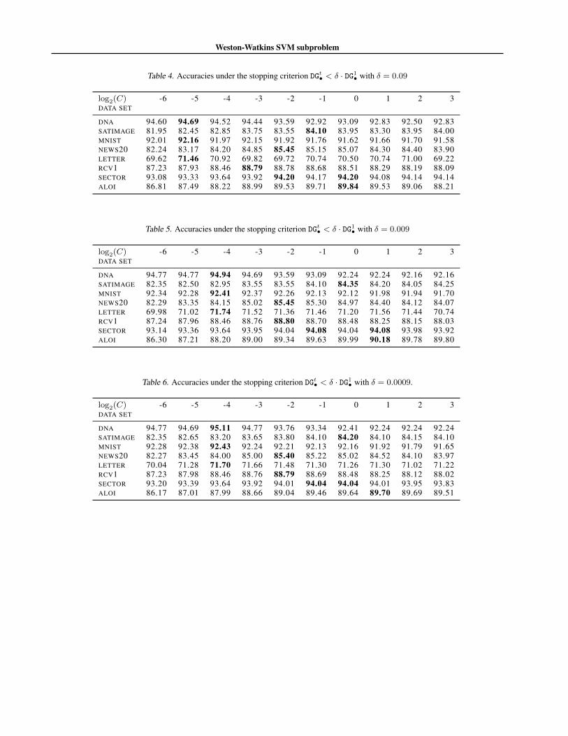
Weston-Watkins SVM subproblem
Table 4. Accuracies under the stopping criterion DGt• < δ · DG1• with δ = 0.09
log2(C) -6 -5 -4 -3 -2 -1 0 1 2 3DATA SET
DNA 94.60 94.69 94.52 94.44 93.59 92.92 93.09 92.83 92.50 92.83SATIMAGE 81.95 82.45 82.85 83.75 83.55 84.10 83.95 83.30 83.95 84.00MNIST 92.01 92.16 91.97 92.15 91.92 91.76 91.62 91.66 91.70 91.58NEWS20 82.24 83.17 84.20 84.85 85.45 85.15 85.07 84.30 84.40 83.90LETTER 69.62 71.46 70.92 69.82 69.72 70.74 70.50 70.74 71.00 69.22RCV1 87.23 87.93 88.46 88.79 88.78 88.68 88.51 88.29 88.19 88.09SECTOR 93.08 93.33 93.64 93.92 94.20 94.17 94.20 94.08 94.14 94.14ALOI 86.81 87.49 88.22 88.99 89.53 89.71 89.84 89.53 89.06 88.21
Table 5. Accuracies under the stopping criterion DGt• < δ · DG1• with δ = 0.009
log2(C) -6 -5 -4 -3 -2 -1 0 1 2 3DATA SET
DNA 94.77 94.77 94.94 94.69 93.59 93.09 92.24 92.24 92.16 92.16SATIMAGE 82.35 82.50 82.95 83.55 83.55 84.10 84.35 84.20 84.05 84.25MNIST 92.34 92.28 92.41 92.37 92.26 92.13 92.12 91.98 91.94 91.70NEWS20 82.29 83.35 84.15 85.02 85.45 85.30 84.97 84.40 84.12 84.07LETTER 69.98 71.02 71.74 71.52 71.36 71.46 71.20 71.56 71.44 70.74RCV1 87.24 87.96 88.46 88.76 88.80 88.70 88.48 88.25 88.15 88.03SECTOR 93.14 93.36 93.64 93.95 94.04 94.08 94.04 94.08 93.98 93.92ALOI 86.30 87.21 88.20 89.00 89.34 89.63 89.99 90.18 89.78 89.80
Table 6. Accuracies under the stopping criterion DGt• < δ · DG1• with δ = 0.0009.
log2(C) -6 -5 -4 -3 -2 -1 0 1 2 3DATA SET
DNA 94.77 94.69 95.11 94.77 93.76 93.34 92.41 92.24 92.24 92.24SATIMAGE 82.35 82.65 83.20 83.65 83.80 84.10 84.20 84.10 84.15 84.10MNIST 92.28 92.38 92.43 92.24 92.21 92.13 92.16 91.92 91.79 91.65NEWS20 82.27 83.45 84.00 85.00 85.40 85.22 85.02 84.52 84.10 83.97LETTER 70.04 71.28 71.70 71.66 71.48 71.30 71.26 71.30 71.02 71.22RCV1 87.23 87.98 88.46 88.76 88.79 88.69 88.48 88.25 88.12 88.02SECTOR 93.20 93.39 93.64 93.92 94.01 94.04 94.04 94.01 93.95 93.83ALOI 86.17 87.01 87.99 88.66 89.04 89.46 89.64 89.70 89.69 89.51

Weston-Watkins SVM subproblem
Table 7. Accuracies under the stopping criterion DGt• < δ · DG1• with δ = 0.09 (first row in each cell), = 0.009 (second row) and= 0.0009 (third row).
log2(C) -6 -5 -4 -3 -2 -1 0 1 2 3DATA SET
DNA (δ = 0.09) 94.60 94.69 94.52 94.44 93.59 92.92 93.09 92.83 92.50 92.83δ = 0.009 94.77 94.77 94.94 94.69 93.59 93.09 92.24 92.24 92.16 92.16δ = 0.0009 94.77 94.69 95.11 94.77 93.76 93.34 92.41 92.24 92.24 92.24
SATIMAGE 81.95 82.45 82.85 83.75 83.55 84.10 83.95 83.30 83.95 84.0082.35 82.50 82.95 83.55 83.55 84.10 84.35 84.20 84.05 84.2582.35 82.65 83.20 83.65 83.80 84.10 84.20 84.10 84.15 84.10
MNIST 92.01 92.16 91.97 92.15 91.92 91.76 91.62 91.66 91.70 91.5892.34 92.28 92.41 92.37 92.26 92.13 92.12 91.98 91.94 91.7092.28 92.38 92.43 92.24 92.21 92.13 92.16 91.92 91.79 91.65
NEWS20 82.24 83.17 84.20 84.85 85.45 85.15 85.07 84.30 84.40 83.9082.29 83.35 84.15 85.02 85.45 85.30 84.97 84.40 84.12 84.0782.27 83.45 84.00 85.00 85.40 85.22 85.02 84.52 84.10 83.97
LETTER 69.62 71.46 70.92 69.82 69.72 70.74 70.50 70.74 71.00 69.2269.98 71.02 71.74 71.52 71.36 71.46 71.20 71.56 71.44 70.7470.04 71.28 71.70 71.66 71.48 71.30 71.26 71.30 71.02 71.22
RCV1 87.23 87.93 88.46 88.79 88.78 88.68 88.51 88.29 88.19 88.0987.24 87.96 88.46 88.76 88.80 88.70 88.48 88.25 88.15 88.0387.23 87.98 88.46 88.76 88.79 88.69 88.48 88.25 88.12 88.02
SECTOR 93.08 93.33 93.64 93.92 94.20 94.17 94.20 94.08 94.14 94.1493.14 93.36 93.64 93.95 94.04 94.08 94.04 94.08 93.98 93.9293.20 93.39 93.64 93.92 94.01 94.04 94.04 94.01 93.95 93.83
ALOI 86.81 87.49 88.22 88.99 89.53 89.71 89.84 89.53 89.06 88.2186.30 87.21 88.20 89.00 89.34 89.63 89.99 90.18 89.78 89.8086.17 87.01 87.99 88.66 89.04 89.46 89.64 89.70 89.69 89.51
A.6.4. COMPARISON WITH CONVEX PROGRAM SOLVERS
For solving (4), we compare the speed of Walrus (Algorithm 2) versus the general-purpose, commercial convex program(CP) solver MOSEK. We generate random instances of the subproblem (4) by randomly sampling v. The runtime resultsof Walrus and the CP solver are shown in Table 8 and Table 9, where each entry is the average over 10 random instances.
Table 8. Runtime in seconds for solving random instances of the problem (4). The parameter C = 1 is fixed while k varies.
log2(k − 1) 2 4 6 8 10 12
WALRUS 0.0009 0.0001 0.0001 0.0001 0.0002 0.0005
CP SOLVER 0.1052 0.0708 0.0705 0.1082 0.5721 12.6057
Table 9. Runtime in seconds for solving random instances of the problem (4). The parameter k = 28 + 1 is fixed while C varies.
log10(C) -3 -2 -1 0 1 2 3
WALRUS 0.0004 0.0001 0.0001 0.0001 0.0001 0.0001 0.0001
CP SOLVER 0.1177 0.1044 0.1046 0.1005 0.1050 0.1127 0.1206
As shown here, the analytic solver Walrus is faster than the general-purpose commercial solver by orders of magnitude.