An economic forecast for the world 2030 - · PDF fileBrazil, Mexico and Russia ... the effects of different ways of running the economy in, for different ... An economic forecast for

Keld Simonsen: An economic forecast for the world 2030

GDP:China

USA

India

1

D E T S A M F U N D S V I D E N S K A B E L I G E F A K U L T E TØ k o n o m i s k I n s t i t u tK Ø B E N H AV N S U N I V E R S I T E T

Kandidatspeciale

Keld Jørn Simonsen

An economic forecast for the world 2030Building a free skeleton for world long time forecasting

Vejleder: Mich Tvede

Afleveret den: 2009-07-22

© Keld Simonsen, 2008. released under the Gnu GFDL licence.


An economic forecast for the world 2030Building a free skeleton for world long time forecasting

It is easy to predict, especially about the future,but whether it will hold trueis a completely other matter

Foreword

The report will give a bid on an economic forecast for the world for the year 2030. A number of problems could then be analysed, such as: Who would be the economic superpower in 2030, India, China, the USA or Europe? What will be the status of Africa, Latin America, and muslim regions? What will happen with the world population and average wages?

To make forecasts, an economic model need to be produced. Initially this may only encompass a few variables, but then the model could be enhanced. This could be with various demographic data such as fertility, and death rates, possibly given for groups of age ranges, for a series of countries and regions. Also included may be economic key data such as GDP. trade balances, employment rates and wage levels. Some outcomes could then be tried out, such as different levels and developments in fertility, mortality, and wage levels.

A special emphasis will be made on the freedom of tools and data. I would like to continue the work after completing the thesis, and then the access to tools and data will most likely be much more restricted than it currently is at the university. For tools, I plan to investigate the statistics package ”R” and a tool from Ib Hansen in the Danish National Bank, and also see if other free tools for economic modelling are available. With respect to data, publicly available sources will be surveyed, although it is expected that UN, IMF and World Bank data series would suffice – given that these series are available eg. on a trial basis to the public. Also other work in the field of longer term world economic forecasts will be researched, including the models employed.

I intend to make the thesis and its model including tools and methods for obtaining data freely available on the web under an open source license, so that others could experiment and refine the work. The open source model is widely used in the computer software world with great results like Linux, Firefox and OpenOffice.org, and it could be interesting to see what this model for development can do for economic models.

2


The model is intended to be time series oriented, and a start could be few key economic and demographic time series for a dozen major regions of the world, including an aggregated world result.

Some factors could later be included for explaining the differences in development:Education: investments in education may really pay off, incl computers for children.religion and culture: Muslim religion may be a hindering factor for growth, strong chinese culture may help in building up a society.

In comparison this version of the document has undergone some changes compared to the delivered version of the thesis. The text has been expanded on a number of issues, including growth theory, measurement issues, other work, statistics, and conclusions. A number of spelling mistakes and language problems has been corrected. Page numbers have been added, and table of contents have been updated with some extra entries.

My motivation for writing this report is that I have done quite some other work on a world scale, including writing a number of software standards for ISO and the IETF, mostly in the areas of cultural diversity support in computer systems, and the internet. So my focus has been very much on the world scene. Furthermore I have been working at University of Copenhagen for a number of years in the 1970ies and 1980ies on maintaining the availability of IMF databases – when these were only available on magnetic tape – so the idea developed then to do a forecast based on these data.

However, I have not received substantial help from my partners of the years of working on IMF tapes when writing this report. And I have not used special material from this work, all material that is used in the report is freely available on the Internet, or as referenced in the bibliography. I have received some help on a number of minor points of the report, as I have discussed it with friends and colleagues and on the R email help list. A special thanks goes to my two supervisors, professor Anders Milhøj and professor Mich Tvede, and to Jesper Ovesen who proofread and came with suggestions for the report.

I have also done much work with the Linux operating system and other open source projects, and I have seen how productive it can be to have many persons from all over the world cooperate freely and voluntarily on a project. This kind of working is not commonplace in the economics scene, and I would like to try to se if the idea can lead to improved productivity also in economics.

Surely, I could have benefited myself in writing this report if I could have used freely the works of others in the area. It is my hope that others may find my work interesting and that they could build on it, to make much more refined models, and use such models to produce much better substantiated results.

3


Table of contentsForeword.................................................................................................................................2Growth and development theory............................................................................................7

Some empirical observations on the growth per capita.....................................................9Convergence.......................................................................................................................9Historic growth and source of growth.............................................................................10Globalization as a development strategy..........................................................................14

Selection of variables............................................................................................................16Previous work in the area......................................................................................................18

Japan Center for Economic Research..............................................................................18Allan Greenspan: The Age of Turbulence......................................................................19Barro and SalaiMartin...................................................................................................19HEIMDAL.......................................................................................................................19United Nations World Population Prospects....................................................................20

Finding the right tools..........................................................................................................21Finding the right data material.............................................................................................22Building the model...............................................................................................................24

Time series naming..........................................................................................................28Getting data into R...........................................................................................................29

Running the model – results and analysis.............................................................................31Estimations of variables...................................................................................................37Population in China, India and USA................................................................................38Total GDP in China, India and USA................................................................................43China, India and USA per capita production...................................................................47The relative roles of USA, EU, China, Asia and Africa..................................................51World population.............................................................................................................52World production per capita............................................................................................54Brazil, Mexico and Russia...............................................................................................55China, Taiwan and Hong Kong........................................................................................56Ireland, Norway and Denmark.........................................................................................57Eastern Europe.................................................................................................................59Africa...............................................................................................................................60Advanced Asia.................................................................................................................61

Describing documenting the work on web...........................................................................62Comparison of results with earlier work..............................................................................63Findings, conclusions and future work.................................................................................65Appendix – log of some R commands.................................................................................67Bibliography.........................................................................................................................86

4


Purpose of the work – hypothesesThe idea of the report is to see what is going to happen in the future, if the current trends in the world economy were to continue. I wanted to see the effects of the trends, in a somewhat longer time range, so that the trends can make some significant effect.

This report is set out to make a forecast for the world economy for the year 2030. I chose the year 2030 as this is something that is quite some years ahead, but still something that I would have a reasonable chance to see in my lifetime. In 2030 I should be retired, so it would also be interesting to see what kind of economic world environment it is likely that I would be experiencing then.

Also forecasts for different countries and regions of the world for 2030 is to be made, including comparisons between various somewhat related economies. This would illustrate the effects of different ways of running the economy in, for different countries.

A specific goal of my work is that I want to continue the work after completing this report, with updated data, and with more elaborate techniques. I also would like to invite others to use my work, so they can make more elaborate work, and maybe we could work together to make better estimations. For that purpose I set another goal, to make the report only with freely available data and tools, preferably open source, so that everybody (including myself) were free to do the work in the future. A goal was then to make a skeleton for world analyses with open source data and tools.

As the world is one of the biggest economic objects to take on, and also for pedagogical reasons and time reasons the idea was to limit the work to only a few basic economic variables. The variables I have chosen to examine are the Gross Domestic Product (GDP), the Gross Domestic product per Capita (GDPPP), and the Population (P). I have initially merely set out to do mere projections of these variables for this report.

The report has a pedagogical angle. Some areas that I hope the work could be used in are:

1. As basis for other scholar work, as a starting point for other students.2. As a basis for teaching3. As a basis for specific sectorial work, like global environment work, pollution or

demographical analysis, where an overall economy estimate is needed.4. I can collect work from others, to make a much more enhanced model

5


5. The enhanced model can be used for testing out policy decisions on a global scale, such as a kind of UN or G20 financial policy, or effects of bigger regional policy decisions in the USA, India, China or EU.

Some issues that I hope to be able to shed some light on are: USA: Heading for bankruptcy?Europe: Stagnation?China: the new emperor?India: the service Goliat.Brazil: Samba to heaven?Middle East: Muslim culture hindering progress?Africa: still in the dark?Korea: one of the tigersJapan: the old industrial wonder.Philippines/Malaysia/Indonesia/Vietnam: on the riseDenmark: land of milk and honey

6


Growth and development theory

The reference B+SiM has an outlay of growth theory, which I use in the following.

The basic neoclassical production function is stated by Solow and Swan, via the form

Y(t) = F ( K(t), L(t), T(t) )

where:

Y(t) is the total production of goods and services at time tK(t) is the level of capital used in the production of Y at time tL(t) is the level of labour used in the production of Y at time tT(t) is the technology level used in the production of Y at time t

A definition of the input variables, and their principal sources of growth:

K Capital represents the durable physical inputs, such as machines, buildings, and so on. The capital goods were produced in the past, as the outcome of a former application of the production function for Y(t). Capital goods also have the characteristic of being a rival good, it cannot be used by several users at the same time.

The capital may accumulate over the years, as not all of Y is consumed, and the depreciation on K may be smaller than the production surplus.

There is a tendency to diminishing returns on capital, that leads to an equilibrium, a steady state.

One part of K is the human capital, which is accumulation of knowledge and thus related to technology. However, it often takes much time (and thus money) to produce human capital, to educate people to a number of tasks, takes many years of school or university attendance, and human capital is a rival good, the same person's knowledge cannot be used by two different producers at the same time.

L Labour represents inputs associated with the human body. It includes such things as the number of workers and the amount of time they work, as well as their physical strength, skills, and health. Labour is a rival good, because a worker cannot work on one activity without reducing the time for another activity.

In this report the population is used as a measure for the labour in one country or region. To get to the real labour component, one then should also take in the other factors, such as employment, rate of men, women and children working, age distribution and their work rates , health and skills, but that data was not available in

7


the data I used on a worldwide scale, and furthermore there would be a problem on how to measure this, also across time.

For longer periods, the population may grow, and thus the amount of labour may increase. Also net effects of immigration and emigration may lead to higher levels of the population. In some regions of the world, like some places in Europe and Russia, the population is declining, and China has a onechildper family policy. So it is not given that population will grow forever. There is a tendency that for higher income countries, fertility is declining, even to at state where the population does not reproduce itself.

T Technology, or knowledge, is the methods employed in the production. Workers and machines cannot produce anything without a formula or blueprint that shows them how to do it, the formula is what is called technology or knowledge. Technology can vary over time for example the same amount of labour and capital produces a larger output in 2000 than in 1900, because the technology used in 2000 is superior. Technology can also differ across countries: the same amount of labour and capital produces a larger output in Japan than in Tanzania, because technology in Japan is better.

The technology most likely improves as knowledge most likely accumulates over time. Sometimes quality production methods are forgotten, but this is not the general trend.

The important aspect of technology is that it is a nonrival good, as two or more producers can use the same formula at the same time.

Technology is in the classical growth analyses taken as exogenous and constant, and as labour given as population growth is also exogenous, and not guaranteed to be positive nor negative, and capital is expected to have diminishing returns approximating zero, then the long term growth is only explained by this exogenous component. It is rather unsatisfactory that growth theory thus is explained by an unexplainable component, but on the other hand it is promising that per capita growth is expected to grow constantly for all future to come.

Fortunately, over the history of time, the world economy has been almost growing all the time, and each of the components K, L, T have also been growing. So economically, we are better off in the world as a whole, as we were a hundred years ago, or a thousand years ago, or ten thousand years ago.

8


Some empirical observations on the growth per capita

Nicolas Kaldor and others have made some observations about what seems to hold about economic growth (B+SiM p 12)

1. Per capita output grows over time, and its growth rate does not tend to diminish2. Physical capital per worker grows over time3. The ratio of physical capital to output is nearly constant4. The shares of labour and physical capital in national income is nearly constant5. The growth rate of output per worker differs substantially across countries6. Poorer countries will grow more than richer countries, but will converge to the growth

rate of the richer countries, when the growth gap is closing

Convergence

There is a general theory on convergence: that the lesser developed countries will catch up with the more developed countries. The more specific specification is called conditional β convergence, that is that the per capita income or production in poorer countries tend to catch up with that of the richer countries, with some conditions set. B+SiM shows that this holds true if you hold constant some factors such as initial levels of human capital, measures of government policies, and the propensities to save and have children. B+SiM claims this relation to be very significant.

Another convergence theory is that factor prices for capital and labour will converge, a part of the HeckscherOhlin model on international trade. This is much what is happening in East Asia, where wages are going up, due to globalization. Globalization is movement of work to areas where the labour is relatively cheaper. This movement of work in facilitated by the use of the Internet and telecommunications, for example software development and customer telephone services can be located to India, which has many persons that can speak English well, and where there have been educated a lot of engineers for the computer industry. Wages in India in the IT industry has then gone up, and there then is a tendency that other countries, such as Vietnam may be a cheaper place to outsource such work.

Another example is the Chinese manufacturing boom, where the manufacturing of many kinds of goods for export have moved many people from the countryside to the cities. Wages have not gone up considerably, though.

9


The convergence of factor prices, especially labour is known to not always hold true. For example the USA is known to export labour intensive goods. Also the conditions mentioned above about the influence of government policies, birth rate, savings rate etc. need to hold true.

Historic growth and source of growth

So what does all this come to, for the countries of the world?

B+SiM has an overview of the economic growth of parts of the last century. Illustrations are taken from B+SiM.

This shows a growth of about 75 % in 30 year. In historic times the last few thousands of years, the production per capita has been ever increasing, except for a few periods with famine or plagues.

10


So there is a wide spread of the income/production per capita, with some African countries in the bottom, some Asian countries next, including China and India, then Latin American countries, and then European and North American countries.

The picture is changing due to different growth rates.

11


Unfortunately some of the poorest countries are also some of those with the smallest growth, such as many African countries, this is in contradiction to a general theory on productivity convergence.

However, the world is getting richer, and even the poor are getting richer, except for Africa.

12


It can be seen that during the last 40 years in all other parts of the world than Africa, poverty has been reduced drastically, in South and East Asia from a level of about 30 % to about 3 %.

What about the convergence of growth rates? One thing is theory, another is what has really happened. B+SiM has figures page 561 onwards. For example the USA surpassed England in the beginning of the 20th century. Argentina and Venezuela were amongst the richest countries in 1870, but are now only at a level of about 25 % of the USA. Australia was 40 % richer than the USA in 1870, but is in 1990 about 25 % poorer. For the period 19001973 India and China were about equal, but in 1987 China were 250 % of India. And many of the lessdeveloped countries, like Bangladesh, India, Indonesia, Pakistan, Philippines, had a decline in GDP per capita Countries improving their relative income per capita include Taiwan, China and South Korea, and Brazil, while other Latin American countries seem to have no change in the relative income. And African countries, some of the poorest of them all, also have a decline in the relative income.

How come? Convergence theory says that poorer countries should approach the income level of the richer countries, but apparently this does not hold true

13


Alan Greenspan has a number of explanations. being a free market evangelist, he speaks much of bureaucratic, governmental hindrances, for example in India, or populistic antiUSA politics in South American countries.

Globalization as a development strategy

I see some trends. H+P claims that development aid does not help. What seems to help, in a big scale, is international trade, and much in the form of globalization.

The production model Y = F(K,L,T) gives special focus to the technology factor as the key factor to growth. Furthermore the technology factor is the key factor to income convergence, it is assumed that the technology is the same all over the world, and that it is a nonrival factor.

Getting the price on the labour factor up and doing the same production in less developed countries, would mean transfer of technology and capital from the more developed countries to the less developed countries. This is exactly what is done with globalization: that companies in more developed countries make subsidiary companies or transfer work to the less developed countries, because of the factor price on the labour factor is less here. In this way, especially when a foreign company creates a subsidiary company in the developing country, transfer of technology and capital, and to some extent also labour is a part of the deal. The technology transfer is mostly carried out by engineers that know the technology. Technology transfer is thus facilitated by government policies of promoting globalization, making it easy to create a company subsidiary in the developing country and have adequate laws for capital transfer in and out of the country and otherwise regulations that make globalization easy, and have a fair amount of locally educated engineers to learn the technology.

Also there should be an adequate ecosystem for the production, such as reasonable skilled and disciplined workforce, no wars, as little corruption as possible, and a legal environment that facilitate the globalization for a foreign company or joint venture.

Such a strategy for a developing country, where the production in the first stages are mainly done for exports, seems to have worked well for a number of countries, such as Taiwan, Hong Kong, China, South Korea, Malaysia, Thailand, Singapore, and even Ireland.

14


In later stages, when the technology transfer has been done to local engineers, and local income has been improved and created a bigger domestic demand for more expensive goods, the emergence of a domestic market for more advanced technologies can happen, and the imported technology can be used for production for the domestic market.

Many of the developing countries are doing a lot of production for exports, which also results in a big trade surplus, and resulting ownership of assets on the importing countries. This does change the distribution of ownership of the production capital for the world.

It could be interesting to investigate how much of the Chinese, Taiwanese and Japanese GDP that is exported netto, mostly to the USA and the EU, and I wonder how long these countries will continue working hard for these foreigners, instead of making products for them selves.

It seems like much effort to improve agricultural production does not lead to much growth, and governments in developing countries should try to play the globalization card.

Is this different to inviting in the foreign countries, that was much accused of imperialism in the 1970ies? I don't know, except that globalization seems to have worked well for the economies mentioned above. Also the focus should be on import of technology, with an emphasis of first making employment and raising the wages of the local people, and later create local businesses and markets.

Some issues are the problems of pollution, energy and global warming, and developing countries should pay special attention to these issues to prevent even bigger problems in the future for them..

15


Selection of variables

The selection of variables for this report is a choice for me between what variables per theory should be significant, and what data series show to be significant, limited to what relevant data series that are available given the requirements for availability of this report, and the limit on the total number of variables that it is viable to work on in this report. In many cases central data is not available on a worldwide basis and in a consistent way, for example it has not been possible for me to find good data on the capital component, including the human capital part.

B+SiM chapter 12 list a number of reasons to explain growth or not. They analyse their data on 112 countries for the 10 and 5 year periods from 1960 to 2000. Their main variable is GDP per capita, so if the total GDP is considered, as in this report, their findings needs to be multiplied with the population figures.

B+SiM suggest in the order of 100 explanatory variables. This is too many variables for a viable model, as it is good practice to limit the number of explanatory variables so that the model explains as much as possible with as few as possible variables.

Given that a reduction of variables is necessary, B+SiM make use of a Bayesian model to estimate the significance and robustness of the variable candidates, and finds about 10 variables (p 553), with related positive or negative effects on growth:

1. + East Asia2. + Primary schooling 19603. Investment price 196019644. GDP 1960 (log)5. Fraction of tropical area6. + Life expectancy in 19607. Latin America or subSaharan Africa8. + Fraction of GDP from mining9. Spanish colony10. + open economy time11. + muslim or buddhist religion12. ethnological fractionalization13. government consumption

The problem is then whether all or some of these variables should be included in this report. I have some doubts about the geographical variables: East Asian, SubSaharan, Latin American, Muslim, Buddhist, tropical area, Spanish colony, as B+SiM at another place say

16


that looking at diverse geographical dummy variables did not explain anything as other variables made the explanatory effects. The geographical dummy variables thus seem to be reflecting other economical variables.

H+P lists another number of variables in their report on whether aid can help developing countries converge to the richer countries’ standard of living. Their conclusion is that aid does not help. So the level of aid will not be analysed in this report. On the other hand they find that there is convergence on the GDP per capita, which is also what B+SiM find.

As mentioned before, in order to make projections of relative GDP levels between countries, demographic data need to be included. This would explain much of the differences in output between say Europe, USA, India and China in 2030.

17


Previous work in the area

Japan Center for Economic Research

The Japan Center for Economic Research has done some work on looking ahead on economy and population till 2050 for major economies of the world. For 2005 and 2030 they report the following figures:

GDP billions GDPPP thousands Population millions

2005 2030 2005 2030 2005 2030

Japan 3470 4710 27.1 40.9 128 115

China 7730 25150 6.8 17.8 1328 1411

Korea 940 1860 19.7 39.5 48 47

India 3380 10390 3.0 6.8 1109 1509

ASEAN 2210 5460 4.6 6.9 385 616

USA 11090 21410 37.2 59.3 298 361

EU 11160 16310 24.8 36.3 449 439

Russia 1390 1890 9.7 15.8 142 119

Brazil 1410 2390 7.5 9.3 186 246

GDP and GDPPP are measured in Purchase Power Parities base year 2000, like also done in this report.

They say they use a homegrown technique for modelling called Successive Approximation, both for their economic and their population outlooks. They say that the UN population forecasts seem to be overestimated, specifically for developed countries, and blame the UN for both doing the estimations and being in charge of programs to reduce world population. They say that total fertility rates are very dependent and declining with advances in per capita income, and that would impact the outlook on population. They use World Bank World Development Indicators data. They say that world population growth rate will fall from 1.3 % today to 1.0 % in 2025 and 0.5 % in 2050. Their analyses include age segments, and they find that all the developed countries will have a much aging population.

18


Their estimation for the economies is that in 2020 China will overcome USA and the EU as the biggest economy in the world.

Allan Greenspan: The Age of Turbulence

Former chief of the US federal bank, Alan Greenspan has written a book titled ”The Age of Turbulence”, where he has published a number of findings for an economic outcast for 2030. In chapter 25 (only) he writes about a forecast, mainly for the USA, and also for a few other countries. He describes the model on page 469 onwards. It is based on number of working hours, calculated on a number of variables are used such as population, age distribution, and employment rate. He estimates an annual growth in working hours of 0.5 %. The then estimates a growth in productivity per hour of 2.2 %, remarkably stable since 1870. He notes though a slip down to 1 % in 2007. He predicts an overall growth rate of 2,5 % based on the hours and productivity estimates, giving a real GDP 75 % higher in 2030 than in 2006.

He also addresses from page 499 onwards other regions of the world, but seemingly without background in time series. Britain he also gives a rosy future. Central Europe will not be as dominating as before because of diminishing population and workforce, Japan likewise. Russia will rise, but it has a long way to go as the GDP per capita is only 1/3 of the Western world. India looks to get much growth, but due to bureaucratic bindings it will be surpassed in growth by China, which doubled its GDP per capita over the last 40 years over India. For China, he leaves it up in the air, dependent on what the politicians of China will allow to happen.

Barro and Sala-i-Martin

B+SiM do list a number of time series for their model work, and has a number of estimations, but no attempt on doing forecasts is made. I am not aware of systematic updates of their data material.

HEIMDAL

HEIMDAL is the Historical Estimated International Model of the DAnish Labour movement.The HEIMDAL model has done work for 13 Western economies, so they have a multinational model. It is a work which was released in 1997, so it is a bit old. It builds on data from the OECD Economic Outlook database, which is updated two times a year. Updated OECD databases exist for 2008, but they are available only on a paid subscription basis.

19


The model has several submodels: the household sector, the business sector, the labour market, domestic prices, foreign sector, public sector and the financial sector. Key explanatory variables are disponible income, interest rate, wages, capital costs, import prices, capacity usage, unemployment, productivity, prices, wage quota, foreign wages, employment, and public and financial sector variables. A number of key variables for each of the sectors are determined.

Each country model has about 100 equations. The countries are related to each other via foreign prices, traded amounts, interest, currency exchange rates and wages. The total set of equations for HEIMDAL in 1997 was 1413 relations and 1155 exogenous variables.

An educational version of the Heimdal model, with data, is available for Danish schools.

United Nations World Population Prospects

The United Nations have done forecasts of the world population, based on individual countries, until 2050. There are numbers from their ”World Population Prospects: The 2008 Revision” for the period that is also covered by this report: Year Millions1980 44371985 48461990 5290 1995 57132000 61152005 65122010 69082015 73022020 76742025 80112030 8308

20


Finding the right tools

As the aim of this report is also to have all results available, so that others can use them, the choice is quite limited.

For the moment I have located 2 tools that may be relevant for the report:

a. The statistical package R. This is a big open source statistical package, which is available in open source, and which has time series capabilities. R is built on the statistical programming language S. A number of tools on top of this are available.

b. Ib Hansen’s econometric package. I have asked for under what conditions this can be made available, and not gotten a clear answer.

Other tools, like SAS, SPSS, STATA, have been excluded as they are only available to the public on a forpay basis. However, there exists open source versions of SAS, called DAP, and of SPSS, called PSPP. These do not enjoy the same level of user support as R.

I have chosen the R package as this is a very big package that is used as a lingua franca in statistics. It has good econometrics support. It seems like very much of the current research in statistics is using R, in international research conferences the majority of talks are using R. R is not used in the education at my economics institute, so help for it has been not so plentiful at my institute.

R is a command line oriented tool, looking like a programming language, which it in fact is. I used the tutorial written by Grant V. Famsworth oriented towards using R in econometrics, and I succeeded in doing my analyses from that tutorial, plus some reading of the R reference documentation plus the help commands of R, so that is a recommendable read, if you want to try running R and the do some analyses. The command line nature of R makes it easy to document what has been done, as R maintains a command log. The command line interface and history makes it easy to repeat previous commands, possibly with small changes. R maintains a data store with all created variables which persists between executions. readily available in a new run. As such I was able to just continue working on old results several months after I did the first calculations. There is a more graphical point and click tool on top of R, called rkward. I have not tried this tool, and I don't know if it is suited for econometric work.

21


Finding the right data material.

Finding data sets that can be used for this project is a major task. The data sets need to be long term, consistent between countries, cover all of the world, and consistent over time.

Providing data in a coherent way on a worldwide basis is a major undertaking. You need to be sure that the same definitions have been used when collecting the data. And as the data is collected from all over the world, and a myriad of series is desirable, there need to be a number of people involved, possibly from each country involved. These people need to have extensive skills in data handling, and economic knowledge. To build a data collection apparatus, that can perform with regularity and consistency, thus take a lot of organisation, and it is only the biggest institutions that can maintain such an apparatus.

Some of these organisations are the International Monetary Fund IMF and the World Bank, both institutions under the United Nations. Other sources could be OECD and agencies of the European Union (EU), the United States of America (USA), and Japan.

The world wide data scene seems to change quite often. So if you are looking for free data then you should regularly check the data providers, especially the ones mentioned above, for new developments in their data offerings.

International Monetary Fund (IMF) has extensive sets of data, available from their web site, This is available in the following series:

IFS: International Financial Statistics

World Trade

The IMF data is available free of charge for a restricted time period. However there seems to be no limit to how many times it is possible to renew the period. There seems to be no restrictions on use of the data.

IMF has issued the IMF data mapper, which contains yearly data since 1980 on key economic indicators. Avilable for download in an excel file.

IMF has issued a data collection World Economic Outlook WEO. The data is free, just like I like it. The focus is very much the same as in this report: data for the world to make forecasts. There is also a web forum for discussion of the WEO project.

The WEO data is available in 2 data sets, both in Microsoft Excel format: one for all countries, and one aggregated for each major region of the world. The data has for each country 33 variables, including Gross Domestic Product, trade balance, debt, inflation, population and unemployment. Data start in 1980. For the aggregated series, 121 series are

22


available, including the above series, and many series on commodity goods such as oil, steel and rice. Data start in 1980 and extend to 2013.

The country series include a series on GDP in national currency that is not deflated, and these series have no counterpart in the aggregate series.

As IMF is predicting figures until 2013, they must have a model for it. I have not been able to get hold on this.

B+SiM list a number of data sets. I have not succeeded in approaching the authors and the publisher to get the status, according to the copyright in the book, and I expect that these data are not regularly updated.

H+P has data, I did contact one of the authors and he said that the article is available from his web page, but I could not find the data there.

The problem with such private data sets is that they are not maintained, so that new data is not readily available.

There is available data via the Institute of Economics, but the data sources are all available on a restricted basis.

The agency CIA in the USA has data.

World Bank worldbank.org

The World Bank WDI World Development Indicators is subscription based, costs USD 200 per year. It covers over 800 development indicators since 1960 for 227 economies.

A smaller set is available for trying out the data, since 1960, for all 227 economies but only about 50 of the most important time series.

It did not look obvious how to retrieve data as time series, but it could possibly be done by some mechanisms.

For this report I chose the IMF WEO data, as it was freely available in a processable form, and the focus of the data was the same as of this report.

23


Building the model

Initially two main economic figures will be examined:

1. Gross Domestic product GDP. This is an indication of the economic power of the country or region in question, and also leads to political power on the world scene, and influence on the whole world economic scenery. The GDP is a main indication of the production of goods and services of a country or region.

2. Gross Domestic Product Per Capita GDPPC. This is an indication of the wealth of each person in the country or region. B+SiM points out that this figure has been constantly improving, with no substantial fallbacks during the last centuries and that is a promising trend – economically it seems like it can only be a better future. Then there are problems, like ”limits to growth”, pollution and scarcity of goods such as oil, financial crises, but in general I think these problems would lead to a slower growth, but still growth will be obtained. Substitutes for oil can be found. We will live in a cleaner world. These factors is not examined in this report, but could be the objects of a refined work.

In the analyses the labour ingredient of the production function will be a major variable, and of course a defining variable of the GDPPC. The labour variable is a quite complex one, which could include skill, health, attitude, working hours, holidays etc. I have chosen the population variable as an estimation of the labour variable, as the labour has to come out of the population and that changes in population is assumed to lead to proportionate changes in labour. If we measure the labour component by the population P we get the equation

GDPPC = GDP / P

Convergence is important, both in the population and also the technology component of the production function. In both instances there is a tendency to convergence for the lesser developed economies towards the figures for the more developed economies. But we cannot assume that they will become asymptotically the same. For example the USA grew out over England in the early 1900, and in the second half of the century Germany outgrew England..

The time series need to be deflated, and also measured in a common currency. The WEO data have series in USD, which is problematic, as the USD has had its own upturns and downturns. The USD exchange rate eg. towards the EUR has fluctuated by over 50 % in the period since

24


1980 till 2009, and the USD has fallen in value towards the EUR about 40 % since 2000. For countries not having a currency strongly related to USD this would mean a growth rate of about 7 %, which is due only to exchange rates, and thus not an indicator of real growth.

The WEO data also has data in ”International dollars” , also known as the GearyKhamis dollar, a term strongly related to Purchasing Power Parity, a term to compensate for that the real cost of products may be different from what to be expected if you just use official currency rates. For example a McDonald's burger may be relatively much cheaper in Portugal compared to Danish prices. The special currency rates for each country to the International dollar is then calculated, using a weighted batch of prices on commodities., which may vary over time. IMF and other international organizations use this artificial currency in some of their time series, as this remedies a number of problems, including the one described above for the USD. The International dollar is a kind of black box currency, which definition is somewhat obscure and maintained by a couple of scientists, but it is well established with the best esteemed economic institutions in the world, such as IMF and the World Bank.

One factor for determining the GDP is the amount of labour employed. This is measured by the population P of the country or region. The population is not an accurate measure of the work force or the labour hours delivered for a given period t, as for example, children, students, pensionists, unemployed and sick people are not subtracted, and changes in working hours are not recorded, but it is assumed that there is a reasonable constant ratio between the population size and the labour hours delivered for a given country or region. The population in each country or region is estimated as part of the model, by a mere ARIMA projection of the population in the countries, and an aggregated world population is estimated out of the projected country populations.

For the neoclassical production function mentioned earlier we thus have some time series that are a reasonable approximation for some of the components, namely GDP for the production Y, and P for the labour component L. I have not found good time series for the capital component K. For the technology component T it is assumed that the growth of technology is constant, which is a reasonable assumption according to B+SiM (and many other growth economists), and the time t is simply taken as a measure for the technology.

To make the predictions even simpler, a number of estimations are done by just projecting the production of the period t as an Arima estimate based on the previous periods. This gives usable estimates, but does not have much relation the the neoclassical production function (you can say that the constant technology growth is included in the time variable, and that the K and L factors are indicated by the previous Y(t) values, but in my mind that is stretching the definitions to a wide extent).

25


In economics we are mostly dealing with terms that can be measured in money. One can dispute if that is so relevant, economists do have an underlying concept of utility to measure, and relations to the money variables. For this report, spanning the 50 years of 1980 to 2030, and other work on longer time scale, such discussion is very relevant. What is it we want to measure, and can we do that consistently over a longer time span? We are said to live in the information age. The very products of Information Technology have a habit of getting cheaper and faster for every year, computers and networking and communications technologies like telephones get cheaper and cheaper. Also Information Age products like music, film, newspapers, TV, radio, (all information content services) get cheaper and cheaper. This trend is expected to continue for the foreseeable future. How can we compare the value of an IT product of today with a product of say ten years ago, or ten years from now? The International Dollar term measures information technology products together with material products like food, and goods. In real terms there will thus be an underestimation of the growth of wealth, because the core technology of the society have these specific attributes of rapid development and ever lower costs.

Furthermore the service products like information content, and also the production capital like programs get a very low reproduction cost. It is easy and very cheap to make a copy of the products and also the capital apparatus. Information technology content goods can actually be seen as nonrival goods, as two producers can use that same source at the same time. In many cases there is negligible production cost, or production and consumption is the same, like downloading a piece of music, and listening to it at the same time, or watching a TV programme. Copying without paying is in many cases not legal due to immaterial law, especially the Berner convention on copyright , but in a major section of the whole business it is legal. One section is the open source software section, which runs much of the backbone of the Internet, and is also viable in the workstation end user market, and the telephone market. Fair use legislation makes it legal to watch, listen to, and copy music and film from TV and radio broadcasts, and in major parts of the world, like China, India and Russia copying freely (by maybe not legally) is the order of the day. In more regulated areas of the world, like Western Europe and the USA, big parts of the population are routinely downloading without paying music and films that they are not allowed to. Some countries like South Korea has made new legislation making such downloading legal. I will expect that there be made more regulations like this all over the world, so that the products of the Information Technology Age will be available to the population at large for the very nominal reproduction cost, that in most cases can be done by the consumers them selves, and that the information content producers can get some payment via some taxes. For the society this would maximize the production of information content products, for a comparatively very small cost. I thus foresee an explosion of the consumption of Information Content products, without anything which looks like a proportionate growth in the GDP.

Given that information technology content products are virtually nonrival goods, there should possibly be special economics for this area. The marginal cost of producing one more copy is virtually nil, or included in the cost of consuming the good, like listening to music over the net, or watching TV or a film over the net.

26


I thus foresee a vast growth of the capabilities of the information age equipment (computers, telephones, network bandwidth etc) and consumption of information age products and services, both without having comparable impact on the GDP. So the growth in GDP and related GDP will be underestimated, and given the importance of these core products and services in the Information Society, this will be a major underestimation of the growth.

The tendency to underestimate growth due to advances in technology will also be present in many other areas of the economy, as technology makes it cheaper to for example produce cars and other goods.

Furthermore, what is it that we want to measure? Since Adam Smith and his wealth of nations it has been one of the economists' major aims to maximize the total wealth of the society. The wealth could be measured in various ways. Many economists have used the market to be a way of maximising production and the underlying utility of the individuals in the society, the utility itself being hard to measure and theoretically impossible to aggregate. One may go a step further to try to maximize the total happiness of the society, which probably has the same difficult characteristics as the utility concept for measuring, comparing and aggregating. But happiness is probably a more core value to humans than utility. So economist and politicians should also have an eye to the happiness measurements. Some happiness measurements are made in the EU and other places on peoples' happiness with life, so it is not completely impossible to measure. Information age technology will lead to cheap access to intellectual property, which for many will enhance their happiness, for example, music, films, books, knowledge in general, better contact with other people, and this to a reproduction cost that is close to nothing. On the other hand, the technology of the information age may be used to watch and control people in a way that may affect their happiness negatively, and it may lead to a society that is controlled centrally, and where secrets are hard to be kept.

The economists settled for mainly maximizing wealth as measured in money terms, and that is what I will also do in this report. You could say that this then only addresses a specific part of human life, but nevertheless, I think it is a very important part, and it is something that we can handle with some certainty.

27


Time series naming.

For an economic analyses data may be obtained from several sources. The different sources may have information on essentially the same economic indicators, but for reasons such as differences in definition, and way of collecting, the data may actually differ. For that reason it is desirable to have the source of the data included in the name of the time series. So the time series naming scheme should be made up from:

1. The source of the data, given by the data bank name. For example WEO not IMFWEO there is no need to specify the institution, when the data bank name is clearly identified.

2. The country or region that the data applies to, ISO 3166 3letter codes are preferable.

3. The name or abbreviation for the time series. It is preferred to keep a naming as close as the name of the source for easy identification.

Fir the time being I actually just use the index number in the two WEO data series, and then for specific analyses I use ad hoc naming. Using the index number was sometimes taken further to having a name – as the ISO 3166 3letter code, plus an offset, using the WEO variable name for the offset name.

For example the name for USA is ”usa” and the name for the world is ”wld”. The offset for the Purchasing Power Parity Per Capita is ”ppppc”. Lowercase names are used as they are easier to type.

28


Getting data into R

The initial trial with the apparatus would be with the IMF WEO data.

I give here a description of my quest for getting the data in a usable form, mostly to warn the reader of where some pitfalls are, so they can be avoided. Readers not interested in working on the data can safely skip this section.

The data was downloaded into two MS Excel files: WEOApr2008all.xls and WEOApr2008alla.xls which were then converted to Comma Separated (.cvs) files WEOApr2008all.csv and WEOApr2008alla.csv via the office application OpenOffice.org. This was later found unnecessary, these files were already in a csv format, with tabulator as the field delimiter. The conversion via OpenOffice.org introduced some problems, such as using the comma as the decimal delimiter. Also semicolons created trouble, these should not be specified as field delimiters in any conversion. I found it misleading to label the data files .xls when they actually were ..csv files. Anyway this did not work either, as somehow the numbers were represented as strings with thousands separators, the comma – USA style, which could not easily be converted to numeric data type, and instead turned up as N/A. Also there were problems interpreting US style thousands separators (comma) – this was then removed in the xls (csv) file. This was then handled via OpenOffice.org, reading it in, saving it as a csv file, editing this and replacing decimal comma (Danish style) with dot, doing these changes made it readable by the read.delim() function of R. I think many of these problems could be avoided by just using an English version of OpenOffice.org

In R the files were then converted into internal R structures via the command:

weoa < read.csv("WEOApr2008alla.xls",header=T,,sep=" ")

Similar for the weo database with all countries.

These were made into time series via the command:

ts(t(as.matrix(weo[,9:42],nrol=34)),start=1980,names=paste("x",weo[,1],".",weo[,2],sep=""))

Make it into a matrix of time series:29


tsw < ts(t(as.matrix(weo[10:43],ncol=34)),start=1980,names=paste("x",weo[,2],".",weo[,3],sep=""))

Convert from character to numeric representation

tsw2 < t( matrix(as.numeric(tsw),ncol=34,byrow=1))

remove IMF estimates:

tsw1 < tsw2[1:28,]

make it into time series again:

tsw3 < ts(tsw2[1:28,],start=1980)

add NA for fitting:

b < cbind(tsw3, matrix(nrow=23,ncol=5975))

I had trouble with this as the data in the time series were character type, where they should be numeric. Various ways of transforming the numbers to numeric were unsuccessful, I tried as.numeric() and data.matrix(). It seems odd that data in time series can be other than numeric. as.numeric() destroyed the dimension aspect of the data, but did convert data to numeric. I then used matrix() to recreate the matrix with correct dimensions,

t( matrix(as.numeric(tswa),ncol=34,byrow=1))

I then tried to do some ordinary least squares analyses via the lm() function.

I used data for the USA, India and China for this, making a model of production Y – measured in international dollars dependent on the labour involved measured by the population L. I did not have data for capital K, so I had to make do with only the L component.

Y = f(L)

So that was the simple model that I set out to investigate.

30


Running the model – results and analysis

Forecasting is easy, but it is done with great uncertainty. For the work at hand predicting into 2030, this is even worse, as predicting so long out in the future may have quite big variation. And the numbers presented in this section of the report should then be taken with all possible precautions.

On the other hand this longer term forecasting gives the opportunity to clearly see the results of trends of the past decades. The trends are strong and unmistakable, as can be seen from the statistical soundness reported in the previous section.

Whether the trends can sustain will of course only be seen in the future. Many things can change the scenario, like global climate crisis, epidemics, economic and natural disasters and war.

Still, I think the scenarios described here are plausible, and thoughtprovoking.

Going on with the work, I then had a look at the estimation of the model. This was first done with the lm() function, to do ordinary Least Squares estimates.

The model to be estimated is:

Y(t) = F(t)

This is a simplification of the model mentioned earlier. The assumption is that the capital and labour factors are constant for each country, and that the technology factor is constant, but also possibly different due to convergence for each country, and that the technology growth is correlated with the time. Furthermore I have no good data for the capital factor. Alternatively one can assume that also the capital and labour components have a constant growth rate correlated with time.

31


I had a look at the GDP, measured in PPP:

ts.plot(tsw3[,usa+pppgdp],tsw3[,ind+pppgdp],tsw3[,chn+pppgdp])

GDP:

USA

China

India

As can be seen these are not really linear, as can be expected for GDP figures. There is normally a growth rate, so the curves are exponential.

32


I then took the logarithmic value of the PPPGDPs:

ts.plot(log(tsw3[,usa+pppgdp]),log(tsw3[,ind+pppgdp]),log(tsw3[,chn+pppgdp]))

log(GDP)

USA

China

India

33


The same was done for the populations (WEO LP)

ts.plot(log(tsw3[,usa+lp]),log(tsw3[,ind+lp]),log(tsw3[,chn+lp]))

log(LP)

China

India

USA

Both the PPPGDP and the LP values now look a lot more linear. I then used the lm() function to make estimates of parameters:

USA:

summary(lm(log(tsw3[,usa+pppgdp]) ~ log(tsw3[,usa+lp])))

34


Call:

lm(formula = log(tsw3[, usa + pppgdp]) ~ log(tsw3[, usa + lp]))

Residuals:

Min 1Q Median 3Q Max

0.1461258 0.0287773 0.0001553 0.0321712 0.0999446

Coefficients:

Estimate Std. Error t value Pr(>|t|)

(Intercept) 20.0759 0.6886 29.16 <2e16 ***

log(tsw3[, usa + lp]) 5.1874 0.1237 41.95 <2e16 ***

Signif. codes: 0 '***' 0.001 '**' 0.01 '*' 0.05 '.' 0.1 ' ' 1

Residual standard error: 0.0575 on 26 degrees of freedom

Multiple Rsquared: 0.9854, Adjusted Rsquared: 0.9849

Fstatistic: 1760 on 1 and 26 DF, pvalue: < 2.2e16

China:

summary(lm(log(tsw3[,chn+pppgdp]) ~ log(tsw3[,chn+lp])))

Call:

lm(formula = log(tsw3[, chn + pppgdp]) ~ log(tsw3[, chn + lp]))

Residuals:

35



0.19056 0.09734 0.01299 0.08383 0.32789

Coefficients:


(Intercept) 67.8590 1.9027 35.66 <2e16 ***

log(tsw3[, chn + lp]) 10.6292 0.2693 39.48 <2e16 ***

Signif. codes: 0 '***' 0.001 '**' 0.01 '*' 0.05 '.' 0.1 ' ' 1




India:

summary(lm(log(tsw3[,ind+pppgdp]) ~ log(tsw3[,ind+lp])))

Call:

m(formula = log(tsw3[, ind + pppgdp]) ~ log(tsw3[, ind + lp]))

Residuals:


0.10217 0.01944 0.00553 0.02505 0.14819

Coefficients:


(Intercept) 21.5842 0.4249 50.79 <2e16 ***

log(tsw3[, ind + lp]) 4.1908 0.0627 66.84 <2e16 ***

36





For all 3 countries the relation was very significant, with a P < 0.001

Estimations of variables

I then tried to make predictions via this lm() method but could not find out how to use the predict() function with the lm() estimation to make forecasts for the coming years. From interrogations I did on the rhelp@rproject.org mailing list it seemed that this was not possible.

I found out that the arima() function could do it. Arima is a BoxJenkins modelling tool, that uses the AutoRegressive Integrated Moving Average technique. Using arima, I could estimate each variable. Arima was also recommended in the tutorial on econometric analyses with R.

The Arima model has 3 parameters ARIMA(p,d,q). where p is the number of autoregressive parameters, d is the number of differentiating passes (lags) over the data, and q is the number of moving average parameters, which are calculated after the differentiating passes. The ARIMA model requires that the input series are stationary, that is that data should have constant mean, standard deviation and autocorrelation over time. The R arima() function automatically checks that a time series is stationary and refuses to give results if the preconditions are not met. Applying different parameters p,d,q to the Arima model should generate very similar results, the model should thus be quite robust to varying parameters..

The Arima technique I have been using is of the order (1,1,2). This means that the moving average is calculated on 1 year's lag.

A question arose about model control in this case. With Arima there is no straight lines estimated as with OLSQ, but you can still draw residual plots for the difference between the observed values and the estimated values.

37

mailto:[email protected]




Population in China, India and USA

Here are the commands to predict populations in China, India and USA:

usa.ml = arima(log(tsw3[,usa+lp]),order=c(1,1,2))

ind.ml = arima(log(tsw3[,ind+lp]),order=c(1,1,2))

chn.ml = arima(log(tsw3[,chn+lp]),order=c(1,1,2))

usa.lp = predict(usa.ml, 23)$pred

ind.lp = predict(ind.ml, 23)$pred

chn.lp = predict(chn.ml, 23)$pred

Population

India

China

USA

ts.plot(tsw3[,usa+lp],tsw3[,ind+lp],tsw3[,chn+lp],exp(usa.lp),exp(ind.lp),exp(chn.lp))

38


From the figure we see that India will overtake China as the most populous nation in about 2020.

We then investigate the residuals for the fitted values to determine the soundness of the regression:

39


India:

Coefficients:

ar1 ma1 ma2

0.9994 0.6287 0.2189

s.e. 0.0035 0.2621 0.2714

sigma^2 estimated as 1.826e05: log likelihood = 106.97, aic = 205.93

40


China:

Coefficients:

ar1 ma1 ma2

0.9928 0.7119 0.2862

s.e. 0.0101 0.2255 0.1965


41


USA:

Coefficients:

ar1 ma1 ma2

0.9950 0.6583 0.3105

s.e. 0.0066 0.1768 0.1721


We see that the data fits reasonably well, with some skewness in the start of the China and USA series, and a downwards slope in the India data. However, the skewness is different for the time series examined, a downwards slope for one series and some tail divergence for the 2 others, and we cannot have different models for different countries, and the deviations are reasonably small, the biggest deviations are about 0.2 % of the fitted values, for all the series..

42


Total GDP in China, India and USA

usa.my = arima(log(tsw3[,usa+pppgdp]),order=c(1,1,2))

chn.my = arima(log(tsw3[,chn+pppgdp]),order=c(1,1,2))

ind.my = arima(log(tsw3[,ind+pppgdp]),order=c(1,1,2))

usa.yp = predict(usa.my, 23)$pred

ind.yp = predict(ind.my, 23)$pred

chn.yp = predict(chn.my, 23)$pred

ts.plot(tsw3[,usa+pppgdp],tsw3[,ind+pppgdp],tsw3[,chn+pppgdp],exp(usa.yp),exp(ind.yp),exp(chn.yp))

43


Here we see that China will overtake the USA in about 10 years time, around 2018, in terms of size of the economy (measured in International Dollars). And we see that India will not catch up significantly with the USA. In 2030 the Chinese economy will be more than twice the size of the economy of the USA.

Does this look plausible? With a population of something like 5 times that of USA, it is not unlikely that Chinese economy will look like this. It is to me more surprising that India is not catching up better.

Residual plots give

China:

44


Coefficients:

ar1 ma1 ma2

0.9996 0.0433 0.8469

s.e. 0.0013 0.1945 0.2143

sigma^2 estimated as 0.000302: log likelihood = 67.84, aic = 127.69

USA:

Coefficients:

ar1 ma1 ma2

0.9976 0.8169 0.0689

s.e. 0.0040 0.3235 0.3205


45


India:

Coefficients:

ar1 ma1 ma2

0.9890 0.0335 0.0859

s.e. 0.0206 0.3519 0.3614


The residuals do not seem to have systematic skewness, so the estimations seem sound.

46


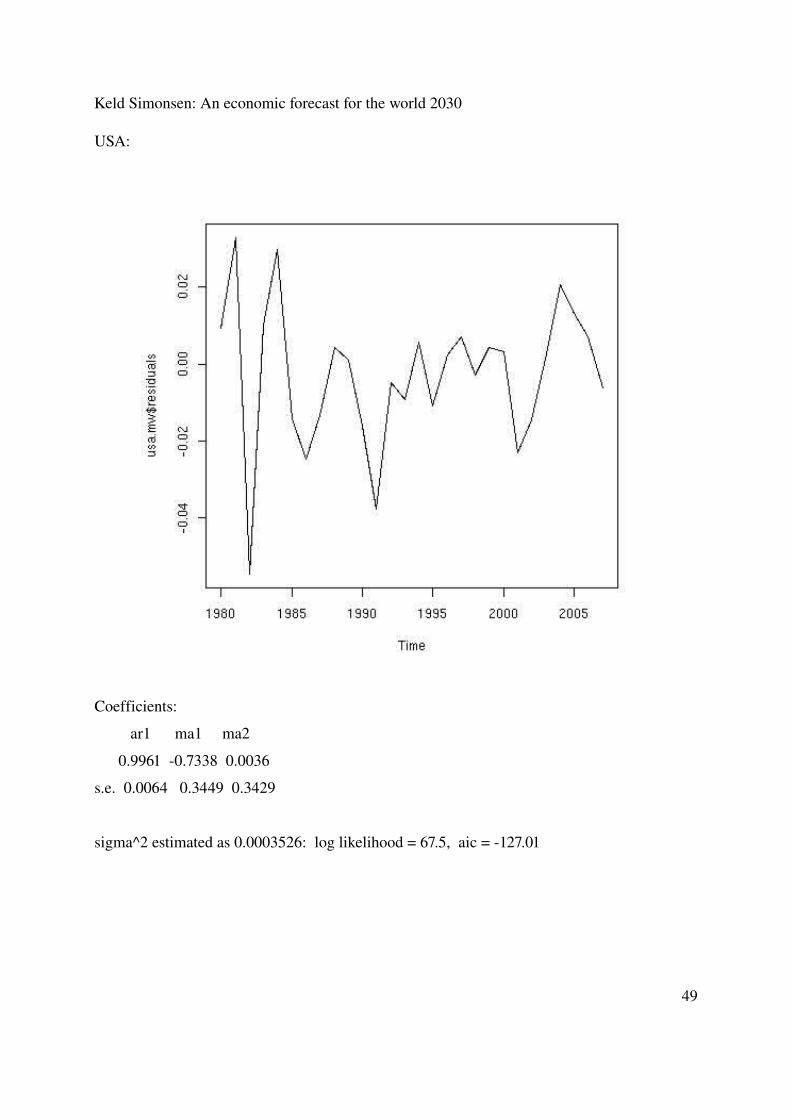
China, India and USA per capita production

Having a look at PPP per capita:

chn.mw = arima(log(tsw3[,chn+ppppc]),order=c(1,1,2))

ind.mw = arima(log(tsw3[,ind+ppppc]),order=c(1,1,2))

usa.mw = arima(log(tsw3[,usa+ppppc]),order=c(1,1,2))

chn.wp = predict(chn.mw, 23)$pred

ind.wp = predict(ind.mw, 23)$pred

usa.wp = predict(usa.mw, 23)$pred

GDPPP

USA

China

India

ts.plot(tsw3[,usa+ppppc],tsw3[,ind+ppppc],tsw3[,chn+ppppc],exp(usa.wp),exp(ind.wp),exp(chn.wp))

47


Assuming that income per person is the same as production per capita, this shows that the Chinese income per person will rise to something like 60 % of the USA income, while income in India will remain low at about 16 % of the USA income, which though is a lot better than the current 6 % of the US figure, and more than 5 times the per capita income in India today.

Residual plots:

China:

Coefficients:

ar1 ma1 ma2

1e+00 0.0248 0.9379

s.e. 2e04 0.2069 0.2078


48


USA:

Coefficients:

ar1 ma1 ma2

0.9961 0.7338 0.0036

s.e. 0.0064 0.3449 0.3429


49


India:

Coefficients:

ar1 ma1 ma2

0.9813 0.1634 0.0597

s.e. 0.0292 0.2749 0.3157


The residual plots do not show any skewness here either. I have not reported residual plots for the rest of the estimations in the report, as that would be using much space, and I cannot change the model for each country or region, they must have the same model, and for the times series where I have done the residual plots, both for the GDP and the GDP per capita, the reported results seem without skewness. Furthermore the report is only reporting possible outcasts, and many things could change, where the statistics are probably the smallest factor.

50


The relative roles of USA, EU, China, Asia and Africa

Using Arima on the aggregated WEO base, on the PPPGPD series we can get the following graph of total production in the respective areas:

GDP:

World

Asia

China

USA/EU

Africa

USA and EU are almost the same. This will hold even if the EU is more populous. It is seen that China is the main contributor to the growth in the world for the next 20 years, and that the developing countries in Asia will account for more than half of the world's economy in 2030, up from about 20 % today. The world will be about 4 times as rich in 2030 as of today.

51


World population

Looking then at the PPPPC, there is no figure for the world in the WEO base. But it can be calculated more or less from the sum of the individual countries. Here there is a problem with missing values for a number of countries, especially in the early period from 1980. I chose to then count the missing values as zero, this gives an estimate that is useful, although biased to have too small initial figures, which will tend to make the growth bigger. With the ARIMA technique, moving averages will help eliminating the bias.

I summed all the populations of the nations:

ix=2+33; wld.lp = tsw3[,2+lp] ; repeat { for (i in 1:28) {wld.lp[i] = sum(tsw3[i,ix+lp],wld.lp[i],na.rm=T);}; ix = ix + 33; if (ix >= 5975) break; }

> wld.lp

Time Series:

Start = 1980

End = 2007

Frequency = 1

[1] 4027.75 4096.19 4169.02 4244.52 4318.98 4397.33 4484.55 4565.64 4642.81

[10] 4871.37 4975.18 5054.24 5284.41 5371.24 5455.02 5534.92 5617.29 5693.15

[19] 5781.95 5859.72 5943.61 6018.93 6117.39 6194.57 6269.58 6346.75 6423.60

[28] 6500.64

This looked reasonable. Estimation via arima() gives:

52


World

population

Which is also reasonable, giving a growth of about 600 million people over 23 years, and growth declining. This is not a population explosion. The world population grew more in the last 25 years than it will do the next 25 years, 2200 million vs 600 million

53


World production per capita

Calculating the PPPPC – income per capita is then done by:

wld.pw = exp(wld.py) / exp(wld.pw)

Which gives:

World

GDPPP

This gives a 4 time growth in average production, or income for all inhabitants of the world. This is mainly due to the big advancements in developing countries like China and India, advanced economies will see growth here under 100 %.

54


Brazil, Mexico and Russia

If we compare Brazil and Mexico as the two biggest latin American countries, with Russia, as the biggest Eastern European country, all built on European culture, and in the middle band of countries, and China, the economic locomotive of the next decades, we get the following, for the PPPPC variable.

GDPPP

China

Russia

Mexico

Brazil

We see that China will surpass these more developed economies in 7 to 15 years. here the phenomenal growth rates of the Chinese economy will make its day. The other economies will not have profound growth, only in the range of 50 to 100 % in the whole period.

55


China, Taiwan and Hong Kong

China, Taiwan, and Hong Kong are all Chinese countries (Hong Kong is a special part of China), and share common Chinese culture. Comparing them wrt. PPPPC – and also USA gives the following:

GDPPP

Hong Kong

Taiwan

USA

China

It seems strange that Hong Kong and Taiwan can surpass the USA, but Hong Kong is already on par with the USA, and being a city state (special part of China) does give them the benefit of city economies, which tend to be above average. Also, having the growth area of the world, Eastern Asia as its close neighbourhood gives both Hong Kong and Taiwan excellent economic opportunities, The USA with its economic problems of trade deficits and slow growth also have a disadvantage in the race here.

56


It is also shown that China, although becoming the economic superpower of the world – still have a lot of room to improve its economy and the welfare of its citizens, as China in 2030 will have less than half of the income per inhabitant as Taiwan.

Ireland, Norway and Denmark

GDPPP

Ireland

Norway

USA

Denmark

China

Ireland, Norway and Denmark are 3 small European countries, each with their special story. Ireland has experienced high growth the last decade, and was in 2007 one of the richest countries in Europe. This was done with a specific industryfriendly set of politics, and some special provisions for the housing market. In the latest year Ireland has experienced substantial economic trouble, but that is not yet reflected in the time series in the available data. Norway has been outside the EU, and has vast income on oil. Denmark has joined the EU, and also has a lot of oil ressources, but the Danish state has not taken control of this as in Norway. Looking at the PPPPC estimates:

57


According to the used data Ireland will here be taking the lead, and already has done so in many respects. Denmark seems to have lost its momentum, and China looks like it will surpass Danish wages in about 30 years time. Norway will keep its pace and have an income more than 50 % higher than Denmark in 2030.

58


Eastern Europe

Eastern Europe has experienced dramatic political changes the last 20 years, going from communist economies dominated by the Soviet Union, to westernstyle economies, and for a number of these countries being members of the EU.

GDPPP

USA

Czech

Latvia

Russia

Ukraine

The former Soviet Union (SU) countries here does not experience so much growth here, while the Czech Republic does, it is about double up for the SU countries, while the Czechs are up for about 200 % growth, and that even on a higher starting point. They do not come even near of the level of USA, and also Western European countries (see analyses of Ireland, Norway, Denmark above).

59


Africa

What will become of Africa? PPPPC analysis again, for the whole of Africa, and then for SubSaharan Africa, compared to the wonder boy of the world, China.

GDPPP

China

Africa

Subsahara

It does not matter here if you live North or South of the Sahara, the development will be roughly the same, a more than 4 fold growth in income. But still nothing compared to the 11fold growth of China.

60


Advanced Asia

Analysing advanced Asia gives the following interesting results

GDPPP

Singapore

Korea

Taiwan

Japan

China

Here it is seen that because of the slow growth in Japanese economy, Singapore, Korea and Taiwan will surpass Japan within the next 25 years, and China will come close to surpassing Japan.

61


Describing documenting the work on web

One aspect of publishing is under which conditions to make the information available. My aim is to make the information available under an open source license, and with a so called viral license, that is, if other people use my work, and publish it, then it must be under the same license. In this way a community around the work can be built, and there is hope that we can together build a model for analysing the effect of world economic policies, which is my ultimate goal, but which is too big for me to undertake as a single person.

Candidates for the license are:

1. The GNU Free Documentation License (GFDL). This license is viral and is used eg. to make the Wikipedia encyclopedia, which is highly successful and one of the world’s primary sources for information. http://en.wikipedia.org/wiki/Wikipedia:Text_of_the_GNU_Free_Documentation_License

2. The Creative Commons license is another set of popular open source licenses, but it is not in general viral.

A further discussion on licenses can be found at http://www.gnu.org/licenses/licenselist.html#DocumentationLicenses

For this work and report, I have chosen the GFDL license, as it suits my purpose, and is well known, and it has been used effectively to create highly successful projects.

For the software produced under this report, I have chosen the GNU General Public License (GPL) http://www.gnu.org/copyleft/gpl.html . This is what I normally do for my software, and I see no reason to chose another license for this project. GPL is one of the most well known licenses in this area and it is viral – which is a property I want, as explained above. The information for this work will be available at the address http://www.dkuug.dk/keld/world2030/

62

http://www.gnu.org/copyleft/gpl.html

http://www.gnu.org/licenses/license-list.html#DocumentationLicenses







Comparison of results with earlier work

With the findings of this report been calculated, I have compared the results with other work in the field as mentioned earlier.

The Japan Center for Economic Research (JCRE) is quite close in subject to the work in this report, both dealing with GDP, GDP per capita and population, as their main variables. Their focus in their report referenced is however the population. They are restricted to a defined set of countries for the economic outlook, mostly Asian countries, and then USA, EU, Russia and Brazil. They use a technique called successive approximation, which sounds a lot like ARIMA, but is more likely a method where they approximate a model of more components for each period, and then continue from there. For example the income level affects the fertility rate, which again affects the income level. I have not been able to find more about the actual method. Their population forecasts are building on more parameters such as age distribution, and womens' work rates, They find many of the same trends as in this report, China will be the economic champion of the world in 2030, India will not overtake USA and EU, the population growth will decline, but it will take until 2050 to reach the 0.5 % level . The growth rates from JCRE and this report are different, and this could be caused by using different data and different models. Especially Japan seems to have a bigger growth by JCRE than in this report.

The Alan Greenspan work is not very elaborate, but well advertised. His calculations are only done as I can see on basis on time series data for the USA. Here he reports a 75 % increase the GDP for 2030. My estimate is a growth of 200 % corresponding to a growth rate of 4.9 %. which is more than I would have expected, but it corresponds to the observed growth rate 19802007 of 5,9 % in PPPGDP for the USA. Greenspan does not make calculations for other countries. Greenspan says that just doing calculations on main economic variables such as GDP and populations makes much sense for longer term forecasts.

The Heimdal model people do not report calculations usinf the model, so there is nothing to compare with. Their model is quite elaborate, but their focus is a bit out of date, mainly focussing on OECD countries. The world has changed and will change even more, as Eastern Asia (excluding Japan) will reach 50 % of the world production in the next 25 years, and also countries like Russia and Brazil will make their mark in the world. It is interesting that Heimdal do try to disseminate their work to schools, I could probably learn much from their methods here, and maybe cooperate with them.

63


B+SiM do not have any predictions , so I cannot compare results. The variables chosen seem to be too specialized to build work on, the Heimdal approach here seems better. Also the data for B+SiM seems to not become updated on a regular basis.

The UN population report has a growth in world population of about 1600 million people, till 2030, where I predict a mere 600 million more inhabitants on this planet. Both estimates are less than the 2200 million I reported as the growth 19802007. My calculations were based on a lower initial population of 4000 million people in 1980 while UN says 4400 million. This should lead to a higher observed growth rate for me and thus to more predicted growth, but the static methods used (ARIMA) predicts a significant lower growth rate, namely 0.5 % compared to the UN figure of 1.0 % The growth rate 19802007 was 1.4 %. Or maybe the ARIMA estimation sees a bigger growth in population in the first part of the time series, because date will emerge here, and then underestimates the growth in the end of the series. Anyway I think the UN population people knows more on this subject than I do.

64


Findings, conclusions and future work

I have achieved what I set out to do. I have successfully gotten hold of data and tools that can be worked on without severe restrictions, and which are gratis to also distribute to other people. I have used the tools and data to do some economic forecasts, with some interesting results – at least to me. Of course the results, being so far in the future, should be taken with a grain (or a ton) of salt, but I believe the trends are true.

Some major findings of this report are:

China will, not surprisingly, be the new emperor of the world. It will overtake the USA and the EU as the biggest economy of the world by about 2018, and by 2030 it will have a GDP of about double the USA GDP. Per capita income will rise about 11 times, approaching about 60 % of USA income, and surpassing a number of other countries in the world.

India will emerge as the most populous country in the world, and will overtake the lead position from China in about 2020, and in 2030 it will be about 300 million more than the 1500 million people in China. However, the per capita income/production growth will be just about 5 times, and thus not gaining much relative importance in the market shares of world production, and not surpass the USA.

The USA will have a 200 % growth in per capita income till 2030.

Brazil and other Latin American countries like Mexico will only enjoy a growth of 110 – 120 %, like Russia.

Africa, both the Muslim area North of Sahara, and the Subsaharan part, will enjoy a 300 % increase in income.

South Korea will overtake Japan in per capita income already in a few years, other East Asian countries will do the same, and even China will overtake Japan in about 2030. More interesting: Singapore, Korea, Hong Kong and Taiwan, in that order, will significantly overtake the USA. Total GDP of what is now regarded as Asian developing countries (including China and India, excluding Japan) will grow from 20 % of the world production in 2007 to 50 % of the world production in 2030.

65


The EU will stay in total GDP on level with the USA. Some countries, including Norway will clearly surpass the USA for the per capita income, while Denmark will stay at a rate 33 % under that of Norway. Some countries in former Eastern Europe, such as the Czech Republic will enjoy a 200 % growth, while Eastern Europe countries outside the EU like Russia and Ukraine will only have a growth of about 100 %.

All in all the world production per capita will have a 4 times increase, and the world population will grow with only 600 million from 6600 million in 2007 to 7200 million in 2030, a mere 0.5 % growth per year, a drop from 1.5 % the preceding 25 years. The population explosion has severely lost pace.

I do find these results very encouraging indeed, and I look forward to my life in 2030!

For future work, of course more economic analyses could be done, including a more elaborate model. Confidence analyses could be introduced. Also many things could be automated in R via functions, and using R in a more clever way. The graphics could be much improved. But the apparatus at hand is a start that can be used to generate quite interesting results.

Working in an educational environment where the tools involved were not very well supported have given some problems, and thus coursed me delays. But then you need to change your habits, and use the open source ways. For example I got good and quick help via the rhelp@rproject.org – I often had response within an hour of my questions. This leads to high bandwidth on that mailing list, but that is of course the consequences. Of course Google and Wikipedia was also an enormous help in my solitary situation.

So may the free economy, and the free economy tools and data live long and prosper, to the benefit of the humanity!

66








Appendix – log of some R commands

Here is the log of some R commands done to do the statistical analyses of this report. This is useful to see how R is used, and also documents the way many of the analyses and the graphs have been conducted. Using the log is very productive when you make similar actions, as you then just can change an existing working command. I also reproduce this as I have been irritated over the lack of disclosure of the methods used in other work. How did they do it? Unfortunately I have not saved all of the history.

weo < read.csv("WEOApr2008alla.csv",header=T,dec=",",sep=" ")

weo < read.csv("WEOApr2008alla.csv",header=T,dec=",",sep=" ")

ts(t(as.matrix(weo[1:4,9:42],nrol=34)),start=1980,names=paste("x",weo[1:4,1],".",weo[1:4,2],sep=""))

tsw= ts(t(as.matrix(weo[1:4,9:42],nrol=34)),start=1980,names=paste("x",weo[1:4,1],".",weo[1:4,2],sep=""))

tsw[7]

dim (tsw)

tsw < ts(t(as.matrix(weo[9:42],nrol=34)),start=1980,names=paste("x",weo[,1],".",weo[,2],sep=""))

dim (tsw)

tsm$x1.ld

tsw$x1.ld

tsw[7]

tsw[7,]

tsw[,7]

tsw[,8]67


tsw[,2]

plot(tsm[,2])

plot(tsw[,2])

plot(tsw[,6])

tsw[,6]

plot(tsw[,7])

tsw[,7]

tsw[,6]

plot(tsw[,6])

plot(tsw[,1])

plot(tsw[,1],tsw[,122]tsw[,243])

plot(tsw[,1],tsw[,122],tsw[,243])

plot(tsw[,1],tsw[,121+1],tsw[,121*2+1],type="1")

plot(tsw[,1])

lines(,tsw[,121+1])

lines(tsw[,121+1])

lines(tsw[,121*2+1])



usa.fit = usapredict(usa.m,usa.fit,n.ahead=23)usa.fitusa.fit = log(usa)predict(usa.m,usa.fit,n.ahead=23)usa.fit?na.actionoptions("na.action")

68


?na.passpredict(usa.m,usa.fit,n.ahead=23)usa.m < lm (log(usa) ~ log(usa.p),na.action =na.pass)usa.m < lm (log(usa) ~ log(usa.p),na.action =na.)dim(usa)usaus = numeric(usa)usus = as.numeric(usa)usus.p = as.numeric(usa.p)us.m = lm( log(us) ~ log(us.p))summary(us.m)predict(us.m)us.m = lm( log(us) ~ log(us.p),na.action=na.exclude)predict(us.m)?arimapredict(us.m,n.ahead=4)names(usa.m)usa.m.na.actionusa.m$na.actionusa.m$fitted.values?lmfit?lsfitus.l =lsfit (log(us), log(us.p))summary(us.l)us.lcoeeficientsus.l$coeeficientsus.l$coeficientsus.l$coefficientsus.l =lsfit (log(us.p), log(us))us.l$coefficientssummary(us.m)predict(us.l,n.count=4)predict(us.m,n.count=4)us = usa[1:28]ususaus.p = usa.p [1:28]us.l = lm(log(us) ~ log(us.p))predict(us.l,n.ahead=5)library(stat)library(stats)us.l = lm(log(us) ~ log(us.p))predict(us.l,n.ahead=5)usa

69


usa.pusus.pus.n = us.pus.l = lm(log(us) ~ log(us.p))predict(us.l,us.n,n.ahead=5)us.nus.n = log(us.p)predict(us.l,us.n,n.ahead=5)us.d = data.frame(us.)predict(us.l,us.d,n.ahead=5)us.dus.p1 = log(us.p)us.y1 = log(us)?lm?predict.lmdata.frame(x = seq(3, 3, 0.5))history()usa.pusausa.m = lm(usa ~ usa.p)usa.d = data.frame(usa.p)predict(usa.m,usa.d,n.count=5)usa.dusausa.ppredict(usa.m,usa.d,n.count=5)predict(usa.m,usa.d,n.count=51)?dynlmlibrary(dynlm)?glslibrary(nlme)?gls?arima.sim?arimapredict.lm(usa.m,usa.d,n.count=51)usa.dusa.pusa.pf = usa.pusa.pf[29:51]=0usa.pfusa.m = lm(usa ~ usa.pf)usa.d = data.frame(usa.pf)usa.m = lm(usa ~ usa.pl)usa.m = lm(usa ~ usa.pf)predict.lm(usa.m,usa.d,n.count=51)m = arima(usa,order=c(1,1,2))

70


predict(m,5)dim (tsw3)chn.ml = arima(tsw3[,1145),order=c(1,1,2))chn.ml = arima(tsw3[,1145],order=c(1,1,2))predict(chn.ml,23)tsw3[,1145]chn.ml = arima(tsw3[,1145],order=c(1,1,2))

predict(chn.ml,23)$predchn.pt = cbind(tsw3[,1145],predict(chn.ml,23)$pred)chn.ptchn.pt = rbind(tsw3[,1145],predict(chn.ml,23)$pred)dim(predict(chn.ml,23)$pred)chn.pt = cbind(tsw3[1,28,1145],predict(chn.ml,23)$pred[1:23])dim(b)b[29:50],1145] =predict(chn.ml,23)$pred[1:23])b[29:50,1145] =predict(chn.ml,23)$pred[1:23])b[29:50,1145] =predict(chn.ml,23)$pred[1:23]b[29:50,1145] =predict(chn.ml,23)$predb[29:50, 1145]predict(chn.ml, 23)$predb[29:50,1145] =predict(chn.ml,23)$pred[1:23]chn.pp = predict(chn.ml, 23)$predtsplot(chn.p,chn.pp)plotts(chn.p,chn.pp)plot.ts(chn.p,chn.pp)?plot.tsts.plot(chn.p,chn.pp)chn.my = arima(tsw3[,1132],order=c(1,1,2))tsw3[,1132]chn.my = arima(log(tsw3[,1132]),order=c(1,1,2))predict(chn.my, 23)$predchn.yp = predict(chn.my, 23)$predchn=1122chn=1124pppgdp=11lp=22usa=5678tsw3[,usa+lp]usa+lplp=21usa+lptsw3[,usa+lp]pppgdp=10tsw3[,usa+pppgdp]tsw3[,usa+pppgdp+1]usa+pppgdptsw3[,usa+pppgdp1]

71


gdpppppppgdppppgdp=9tsw3[,usa+pppgdp]ind=2444ind.my = arima(log(tsw3[,ind+pppgdp]),order=c(1,1,2))indind.yp = predict(ind.my, 23)$predusa.my = arima(log(tsw3[,usa+pppgdp]),order=c(1,1,2))usa.yp = predict(usa.my, 23)$predusa.ml = arima(log(tsw3[,usa+lp]),order=c(1,1,2))ind.ml = arima(log(tsw3[,ind+lp]),order=c(1,1,2))chn.ml = arima(log(tsw3[,chn+lp]),order=c(1,1,2))usa.lp = predict(usa.ml, 23)$predind.lp = predict(ind.ml, 23)$predchn.lp = predict(chn.ml, 23)$predts.plot(exp(usa.yp),exp(ind.yp),exp(chn.up))ts.plot(exp(usa.yp),exp(ind.yp),exp(chn.yp))chn.lp = predict(chn.ml, 30)$predind.lp = predict(ind.ml, 30)$predusa.lp = predict(usa.ml, 30)$predusa.yp = predict(usa.my, 23)$predusa.yp = predict(usa.my, 30)$predind.yp = predict(ind.my, 30)$predchn.yp = predict(chn.my, 30)$predts.plot(exp(usa.yp),exp(ind.yp),exp(chn.yp))tsw3[,ind+pppgdp]tsw3[,chn+pppgdp]tsw3[,usa+pppgdp]ind+pppgdpchn+pppgdppppgdppppgdp=8tsw3[,usa+pppgdp]tsw3[,usa+pppgdp]tsw3[,chn+pppgdp]tsw3[,ind+pppgdp]usa.my = arima(log(tsw3[,usa+pppgdp]),order=c(1,1,2))ind.my = arima(log(tsw3[,ind+pppgdp]),order=c(1,1,2))chn.my = arima(log(tsw3[,chn+pppgdp]),order=c(1,1,2))ts.plot(exp(usa.yp),exp(ind.yp),exp(chn.yp))ind.yp = predict(ind.my, 30)$predchn.yp = predict(chn.my, 30)$predusa.yp = predict(usa.my, 23)$predusa.yp = predict(usa.my, 30)$predts.plot(exp(usa.yp),exp(ind.yp),exp(chn.yp))ts.plot(tsw3[,usa+pppgdp],tsw3[,ind+pppgdp],tsw3[,chn+pppgdp],exp(usa.yp),exp(ind.yp),exp(chn.yp))

72


usa.yp = predict(usa.my, 23)$predchn.yp = predict(chn.my, 23)$predind.yp = predict(ind.my, 23)$predts.plot(tsw3[,usa+pppgdp],tsw3[,ind+pppgdp],tsw3[,chn+pppgdp],exp(usa.yp),exp(ind.yp),exp(chn.yp))ts.plot(log(tsw3[,usa+pppgdp]),log(tsw3[,ind+pppgdp]),tsw3[,log(chn+pppgdp]))ts.plot(log(tsw3[,usa+pppgdp]),log(tsw3[,ind+pppgdp]),log(tsw3[,chn+pppgdp]))yn =0ts.plot(log(tsw3[,usa+yn]),log(tsw3[,ind+yn]),log(tsw3[,chn+yn]))tsw3[,chn+yn]tsw3[,ind+yn]yn=1ts.plot(log(tsw3[,usa+yn]),log(tsw3[,ind+yn]),log(tsw3[,chn+yn]))tsw3[,ind+yn]tsw3[,chn+yn]tsw3[,usa+yn]ppppc=pppgdp+1ts.plot(log(tsw3[,usa+ppppc]),log(tsw3[,ind+ppppc]),log(tsw3[,chn+ppppc]))ts.plot(tsw3[,usa+ppppc],tsw3[,ind+ppppc],tsw3[,chn+ppppc])plot.ts(tsw3[,usa+ppppc],tsw3[,ind+ppppc],tsw3[,chn+ppppc])?plot.ts?ts.polt?ts.plotjpeg("out.jpg")o = dev.off()osa =jpeg("out.jpg")sb =ots.plot(tsw3[,usa+pppgdp],tsw3[,ind+pppgdp],tsw3[,chn+pppgdp])sats.plot(tsw3[,usa+pppgdp],tsw3[,ind+pppgdp],tsw3[,chn+pppgdp])sbts.plot(tsw3[,usa+pppgdp],tsw3[,ind+pppgdp],tsw3[,chn+pppgdp])jpeg("out.jpg")ts.plot(tsw3[,usa+pppgdp],tsw3[,ind+pppgdp],tsw3[,chn+pppgdp])dev.off()ts.plot(log(tsw3[,usa+pppgdp]),log(tsw3[,ind+pppgdp]),log(tsw3[,chn+pppgdp]))jpeg("out.jpg")ts.plot(log(tsw3[,usa+pppgdp]),log(tsw3[,ind+pppgdp]),log(tsw3[,chn+pppgdp]))dev.off()

73


ts.plot(log(tsw3[,usa+pl]),log(tsw3[,ind+pl]),log(tsw3[,chn+pl]))lpts.plot(log(tsw3[,usa+lp]),log(tsw3[,ind+lp]),log(tsw3[,chn+lp]))jpeg("out.jpg")ts.plot(log(tsw3[,usa+lp]),log(tsw3[,ind+lp]),log(tsw3[,chn+lp]))dev.off()model = lm(log(tsw3[,usa+lp]) ~ log(tsw3[,usa+lp]))model = lm(log(tsw3[,usa+pppgdp]) ~ log(tsw3[,usa+lp]))summary(model)summary(model = lm(log(tsw3[,usa+pppgdp]) ~ log(tsw3[,usa+lp])))summary(model = lm(log(tsw3[,usa+pppgdp]) ~ log(tsw3[,usa+lp])))summary(lm(log(tsw3[,usa+pppgdp]) ~ log(tsw3[,usa+lp])))summary(lm(log(tsw3[,chn+pppgdp]) ~ log(tsw3[,chn+lp])))summary(lm(log(tsw3[,ind+pppgdp]) ~ log(tsw3[,ind+lp])))?savehistoryhistory(max.show =200)history(max.show =200)ts.plot(tsw3[,usa+pppgdp],tsw3[,ind+pppgdp],tsw3[,chn+pppgdp],exp(usa.yp),exp(ind.yp),exp(chn.yp))jpeg("out.jpg")ts.plot(tsw3[,usa+pppgdp],tsw3[,ind+pppgdp],tsw3[,chn+pppgdp],exp(usa.yp),exp(ind.yp),exp(chn.yp))dev.off()ts.plot(tsw3[,usa+lp],tsw3[,ind+lp],tsw3[,chn+lp],exp(usa.lp),exp(ind.lp),exp(chn.lp))jpeg("out.jpg")ts.plot(tsw3[,usa+lp],tsw3[,ind+lp],tsw3[,chn+lp],exp(usa.lp),exp(ind.lp),exp(chn.lp))dev.off()ts.plot(tsw3[,usa+ppppc],tsw3[,ind+ppppc],tsw3[,chn+ppppc])usa.my = arima(log(tsw3[,usa+pppgdp]),order=c(1,1,2))chn.my = arima(log(tsw3[,chn+pppgdp]),order=c(1,1,2))ind.my = arima(log(tsw3[,ind+pppgdp]),order=c(1,1,2))usa.yp = predict(usa.my, 23)$predind.yp = predict(ind.my, 23)$predchn.yp = predict(chn.my, 23)$predchn.mw = arima(log(tsw3[,chn+ppppc]),order=c(1,1,2))ind.mw = arima(log(tsw3[,ind+ppppc]),order=c(1,1,2))usa.mw = arima(log(tsw3[,usa+ppppc]),order=c(1,1,2))chn.wp = predict(chn.mw, 23)$predind.wp = predict(ind.mw, 23)$predusa.wp = predict(usa.mw, 23)$pred

74


ts.plot(tsw3[,usa+ppppc],tsw3[,ind+ppppc],tsw3[,chn+ppppc],exp(usa.wp),exp(ind.wp),exp(chn.wp))jpeg("out.jpg")ts.plot(tsw3[,usa+ppppc],tsw3[,ind+ppppc],tsw3[,chn+ppppc],exp(usa.wp),exp(ind.wp),exp(chn.wp))dev.off()exp(chn.wp)exp(usa.wp)exp(ind.wp)tswa[,7]tswa[,6]2927.959/ 47852.3716468.951/ 117823.3516468.951/2927.95969751.252/117823.35wld=2eur=728afr=970mea=1696asi=1454y=5tswa[,wld+y]y=4tswa[,wld+y]tswa[,asi+y]tswa[,eur+y]tswa[,afr+y]tswa[,mea+y]historyhistory()amr=1817amr.my = arima(log(tswa[,amr+y]),order=c(1,1,2))dim(tswa3)tswa2 < t( matrix(as.numeric(tswa),ncol=34,byrow=1))tswa3 < ts(tswa2[1:28,],start=1980)amr.my = arima(log(tswa3[,amr+y]),order=c(1,1,2))ts.plot(tswa3[, amr + y])asi.my = arima(log(tswa3[,asi+y]),order=c(1,1,2))eur.my = arima(log(tswa3[,eur+y]),order=c(1,1,2))afr.my = arima(log(tswa3[,afr+y]),order=c(1,1,2))asi.my = arima(log(tswa3[,asi+y]),order=c(1,1,2))ts.plot(tswa3[, asi + y])tswa3[, asi + y]tswa3[1, asi + y]= 886.531ts.plot(tswa3[, asi + y])asi.my = arima(log(tswa3[,asi+y]),order=c(1,1,2))tswa3[, amr + y]amr.my = arima(log(tswa3[,amr+y]),order=c(1,1,2))

75


wld.my = arima(log(tswa3[,wld+y]),order=c(1,1,2))ts.plot(tswa3[, amr + y])eur.py = predict(eur.my, 23)$predamr.py = predict(amr.my, 23)$predasi.py = predict(asi.my, 23)$predafr.py = predict(afr.my, 23)$predmea.py = predict(mea.my, 23)$predmea.my = arima(log(tswa3[,mea+y]),order=c(1,1,2))wld.my = arima(log(tswa3[,wld+y]),order=c(1,1,2))wld.py = predict(wld.my, 23)$predts.plot(wld.py,afr.py,asi.py,eur.py)ts.plot(wld.py,afr.py,asi.py,eur.py,amr.py)ts.plot(wld.py,asi.py,eur.py,amr.py)ts.plot(wld.py,amr.py)ts.plot(wld.py,eur.py)tswa3[,eur+y]tswa3[,amr+y]usa.ypexp(usa.yp)exp(eur.py)exp(amr.py)tswa3[,amr+y]tswa3[,eur+y]ts.plot(wld.py,amr.py)ts.plot(wld.py,asi.py)ts.plot(exp(wld.py),exp(asi.py))ts.plot(exp(wld.py),exp(asi.py),exp(eur.py),exp(usa.yp),exp(afr.py))ts.plot(exp(wld.py),exp(asi.py),exp(eur.py),exp(usa.yp),exp(afr.py),exp(chn.yp))jpeg("out.jpg")ts.plot(exp(wld.py),exp(asi.py),exp(eur.py),exp(usa.yp),exp(afr.py),exp(chn.yp))dev.off()exp(asi.py)exp(wld.py)158388.45/285960.7614561.85/69215.93285960.76/69215.93exp(afr.py)10778.368/2209.824wld.pl = tsw3(2)ix =2wld.pl = tsw3(ix+pl)wld.pl = tsw3[,ix+pl]pllpwld.pl = tsw3[,ix+lp]

76


dim(tsw3)repeatif (ix > 5975) breakixrepeat { if (ix > 5975) break; ix = ix + 33; wld.pl = tsw3[,ix+lp] + wld.pl; }ixix=2; wld.lp = 0; repeat { wld.lp = tsw3[,ix+lp] + wld.lp; ix = ix + 33; if (ix >= 5975) break; }wld.lpix=2+33; wld.lp = tsw3[,2+lp] ; repeat { wld.lp = tsw3[,ix+lp] + wld.lp; ix = ix + 33; if (ix >= 5975) break; }ixwld.lpwld.lp = tsw3[,2+lp]wld.lphelp.search("na")help.search("na")?na?substitutenahelp.search("substitutena")?substitute?na.omit?na.action?optionoptions("na.action")?options("na.action")?na.actionna.action(tswa3)na.action(tswa3)=na.omitts0 = tswa3dim(ts0)for (i in 1:28) for (j in 1:ts0 = tsw3dim(ts0)for (i in 1:28) for (j in 1:5975) { if (ts0[i,j] == NA ] ts0[i,j] =0;}for (i in 1:28) for (j in 1:5975) { if (ts0[i,j] == NA ) ts0[i,j] =0;}for (i in 1:28) for (j in 1:5975) { if (ts0[i,j] = NA ) ts0[i,j] =0;}?ifhelp(if)help("if")for (i in 1:28) for (j in 1:5975) { if (!ts0[i,j] ) ts0[i,j] =0;}for (i in 1:28) for (j in 1:5975) { if (!ts0[i,j] ) {ts0[i,j] =0;}}

77


a = NAaif (!a) aif (!a) { a}if (!a) { a= 3}if (a) { a= 3}if (a> 2) { a= 3}help("if")syntaxSyntaxhelp("Syntax")for (i in 1:28) {for (j in 1:5975) { if (!ts0[i,j] ) {ts0[i,j] =0;}}}ts0[5,22]for (i in 1:28) {for (j in 1:5975) { if (ts0[i,j] == NA ) {ts0[i,j] =0;}}}idn=2477mex=3500rus=4358dnk=1454twn=5183bra=728hkg=2345tsa3[,dnk+lp]tsw3[,dnk+lp]history(max.show=299)dnk.ml = arima(log(tsw3[,dnk+lp]),order=c(1,1,2))dnk.mw = arima(log(tsw3[,dnk+ppppc]),order=c(1,1,2))twn.mw = arima(log(tsw3[,twn+ppppc]),order=c(1,1,2))twn.ml = arima(log(tsw3[,twn+lp]),order=c(1,1,2))hkg.mw = arima(log(tsw3[,hkg+ppppc]),order=c(1,1,2))h =history(max.show=299)hh()h <history(max.show=299)hh()history(max.show=299)bra.ml = arima(log(tsw3[,bra+lp]),order=c(1,1,2))bra.mw = arima(log(tsw3[,bra+ppppc]),order=c(1,1,2))mex.mw = arima(log(tsw3[,mex+ppppc]),order=c(1,1,2))tsw3[,mex+ppppc]ts.plot(tsw3[,mex+ppppc])ts.plot(tsw3[,bra+ppppc])ts.plot(tsw3[,bra+ppppc],tsw3[,mex+ppppc])rus.mw = arima(log(tsw3[,rus+ppppc]),order=c(1,1,2))history(max.show=299)mex.pw = predict(mex.mw, 23)$pred

78


rus.pw = predict(rus.mw, 23)$predbra.pw = predict(bra.mw, 23)$predts.plot(exp(chn.pw),exp(rus.pw),exp(bra.pw),exp(mex.pw))bra.pw = predict(chn.mw, 23)$predbra.pw = predict(bra.mw, 23)$predchn.pw = predict(chn.mw, 23)$predts.plot(exp(chn.pw),exp(rus.pw),exp(bra.pw),exp(mex.pw))history(max.show=299)jpeg("out.jpg")ts.plot(exp(chn.pw),exp(rus.pw),exp(bra.pw),exp(mex.pw))dev.off()twn.pw = predict(twn.mw, 23)$predhkg.pw = predict(hkg.mw, 23)$predts.plot(exp(chn.pw),exp(hkg.pw),exp(twn.pw))ts.plot(exp(chn.pw),exp(hkg.pw),exp(twn.pw),exp(usa.pw))usa.pw = predict(usa.mw, 23)$predts.plot(exp(chn.pw),exp(hkg.pw),exp(twn.pw),exp(usa.pw))ts.plot(exp(chn.pw),exp(hkg.pw),exp(twn.pw),exp(usa.pw))usa.pwhkg.pwtwn.pwjpeg("out.jpg")ts.plot(exp(chn.pw),exp(hkg.pw),exp(twn.pw),exp(usa.pw))dev.off()history(max.show=299)irl=2543irl.mw = arima(log(tsw3[,irl+ppppc]),order=c(1,1,2))irl.pw = predict(irl.mw, 23)$prednor=3962nor.mw = arima(log(tsw3[,+ppppc]),order=c(1,1,2))nor.pw = predict(nor.mw, 23)$predts.plot(exp(chn.pw),exp(nor.pw),exp(irl.pw),exp(dnk.pw))dnk.pw = predict(dnk.mw, 23)$predts.plot(exp(chn.pw),exp(nor.pw),exp(irl.pw),exp(dnk.pw),exp(usa.pw))exp(usa.pw)exp(dnk.pw)ts.plot(exp(chn.pw),exp(nor.pw),exp(irl.pw),exp(dnk.pw),exp(usa.pw))

a = NA; if (a == NA) { a = 0}

?sum

ix=2; wld.lp = 0; repeat { wld.lp = sum(tsw3[,ix+lp],wld.lp,na.rm=T); ix = ix + 33; if (ix >= 5975) break; }

79


wld.lp

ix=2+33; wld.lp = tsw3[,2+lp] ; repeat { wld.lp = sum(tsw3[,ix+lp],wld.lp,na.rm=T); ix = ix + 33; if (ix >= 5975) break; }

wld.lp

wld.lp = tsw3[,2+lp]

wld.lp

ix=2+33

wld.lp = sum(tsw3[,ix+lp],wld.lp,na.rm=T)

wld.lp

ix=2+33; wld.lp = tsw3[,2+lp] ; repeat { for (i in 1:28) {wld.lp[i] = sum(tsw3[i,ix+lp],wld.lp[i],na.rm=T); ix = ix + 33; if (ix

>= 5975) break; }

wld.lp

ix=2+33; wld.lp = tsw3[,2+lp] ; repeat { for (i in 1:28) {wld.lp[i] = sum(tsw3[i,ix+lp],wld.lp[i],na.rm=T);} ix = ix + 33; if (ix

>= 5975) break; }

ix=2+33; wld.lp = tsw3[,2+lp] ; repeat { for (i in 1:28) {wld.lp[i] = sum(tsw3[i,ix+lp],wld.lp[i],na.rm=T);}; ix = ix + 33; if (i

x >= 5975) break; }

wld.lp

wld.ml = arima(log(wld.lp),order=c(1,1,2))

log(wld.lp)

wld.pl = predict(wld.ml, 23)$pred

wld.pw = wld.py / wld.pl

80


ts.plot(exp(wld.pl))

wld.pw = wld.py / exp(wld.pl)

ts.plot(wld.pw)

wld.py

tswa[,wld+y]

tswa3[,wld+y]

wld.pw = exp(wld.py) / exp(wld.pw)

ts.plot(wld.pw)

exp(wld.py)

jpeg("out.jpg")

ts.plot(exp(wld.pl))

dev.off()

exp(wld.pl)

jpeg("out.jpg")

ts.plot(wld.pw)

dev.off()

wld.pw

pol=4226

svn=4724

ukr=5579

rou=4325

pol.mw = arima(log(tsw3[,pol+ppppc]),order=c(1,1,2))

tsw3[,pol+ppppc]

ukr.mw = arima(log(tsw3[,ukr+ppppc]),order=c(1,1,2))

81


rou.mw = arima(log(tsw3[,rou+ppppc]),order=c(1,1,2))

svn.mw = arima(log(tsw3[,svn+ppppc]),order=c(1,1,2))

bgr=793

cze=1421

cze.mw = arima(log(tsw3[,cze+ppppc]),order=c(1,1,2))

lva=2972

lva.mw = arima(log(tsw3[,lva+ppppc]),order=c(1,1,2))

lva.pw = predict(lva.mw, 23)$pred

cze.pw = predict(cze.mw, 23)$pred

ukr.pw = predict(ukr.mw, 23)$pred

rou.pw = predict(rou.mw, 23)$pred

ts.plot(exp(usa.pw),exp(cze.pw),exp(ukr.pw),exp(lva.pw))

ts.plot(exp(usa.pw),exp(cze.pw),exp(ukr.pw),exp(lva.pw),exp(rus.pw))

exp(ukr.pw)

exp(rus.pw)

wld.pw

pol=4226

svn=4724

ukr=5579

rou=4325

pol.mw = arima(log(tsw3[,pol+ppppc]),order=c(1,1,2))

tsw3[,pol+ppppc]

ukr.mw = arima(log(tsw3[,ukr+ppppc]),order=c(1,1,2))

rou.mw = arima(log(tsw3[,rou+ppppc]),order=c(1,1,2))

82


svn.mw = arima(log(tsw3[,svn+ppppc]),order=c(1,1,2))

bgr=793

cze=1421

cze.mw = arima(log(tsw3[,cze+ppppc]),order=c(1,1,2))

lva=2972

lva.mw = arima(log(tsw3[,lva+ppppc]),order=c(1,1,2))

lva.pw = predict(lva.mw, 23)$pred

cze.pw = predict(cze.mw, 23)$pred

ukr.pw = predict(ukr.mw, 23)$pred

rou.pw = predict(rou.mw, 23)$pred

ts.plot(exp(usa.pw),exp(cze.pw),exp(ukr.pw),exp(lva.pw))


exp(ukr.pw)

exp(rus.pw)

exp(lva.pw)

exp(cze.pw)

jpeg("out.jpg")


dev.off()

sah=1091

sah.mw = arima(log(tswa3[,sah+y]),order=c(1,1,2))

sah.pw = predict(sah.mw, 23)$pred

ts.plot(exp(afr.pw),exp(sah.pw)exp(chn.pw))

83


ts.plot(exp(afr.pw),exp(sah.pw),exp(chn.pw))

afr.mw = arima(log(tswa3[,afr+y]),order=c(1,1,2))

afr.pw = predict(afr.mw, 23)$pred


chn.pw = predict(chn.mw, 23)$pred


jpeg("out.jpg")


dev.off()

afr.pw

exp(afr.pw )

chn.pw

exp(chn.pw )

jpn=2675

sgp=4655

kor=2840

kor.mw = arima(log(tsw3[,kor+ppppc]),order=c(1,1,2))

jpn.mw = arima(log(tsw3[,jpn+ppppc]),order=c(1,1,2))

sgp.mw = arima(log(tsw3[,sgp+ppppc]),order=c(1,1,2))

84


sgp.pw = predict(sgp.mw, 23)$pred

jpn.pw = predict(jpn.mw, 23)$pred

kor.pw = predict(kor.mw, 23)$pred

ts.plot(exp(twn.pw),exp(sgp.pw),exp(jpn.pw),exp(kor.pw),exp(chn.pw))

exp(twn.pw)

exp(sgp.pw)

exp(jpn.pw)

exp(chn.pw)

exp(kor.pw)

jpeg("out.jpg")

ts.plot(exp(twn.pw),exp(sgp.pw),exp(jpn.pw),exp(kor.pw),exp(chn.pw))

dev.off()

jpeg("out.jpg"); ts.plot(chn.ml$residuals); dev.off() jpeg("out.jpg"); ts.plot(ind.ml$residuals); dev.off() jpeg("out.jpg"); ts.plot(usa.ml$residuals); dev.off() jpeg("out.jpg"); ts.plot(chn.my$residuals); dev.off() jpeg("out.jpg"); ts.plot(usa.my$residuals); dev.off() jpeg("out.jpg"); ts.plot(ind.my$residuals); dev.off() jpeg("out.jpg"); ts.plot(chn.mw$residuals); dev.off() jpeg("out.jpg"); ts.plot(usa.mw$residuals); dev.off() jpeg("out.jpg"); ts.plot(ind.mw$residuals); dev.off()

85


Bibliography

B+SiM: Barro, Robert S.; SalaiMartin, Xavier: Economic Growth, MIT Press, Cambridge, 2004.

H+P: Herbertson, Tryggvi Thor; Paldam, Martin: Does development aid help poor countries converge to our standard of living? Nationaløkonomisk Tidsskrift 145 (2007) p 188214

Grant V. Farnsworth: Econometrics in Rhttp://cran.rproject.org/doc/contrib/FarnsworthEconometricsInR.pdf

Japan Center for Economic Research: World Economic and Population Outlook 20062050http://www.jcer.or.jp/eng/pdf/2006long_contents.pdfhttp://www.jcer.or.jp/eng/pdf/2006long_table.pdf

United nations Population Prospectshttp://esa.un.org/unpp

Alan Greenspan: The age of turbulence – Adventures in a new world. Penguin Press, London, 2007.

Heimdal Historical Estimated International Model of the DAnish Labour movement (in Danish), 1997http://www.aeraadet.dk/media/filebank/org/HEISLUT.PDF

Wikipedia, various articleshttp://wikipedia.org

86

http://www.aeraadet.dk/media/filebank/org/HEI-SLUT.PDF

http://esa.un.org/unpp

http://www.jcer.or.jp/eng/pdf/2006long_table.pdf

http://cran.r-project.org/doc/contrib/Farnsworth-EconometricsInR.pdf

Documents

An economic forecast for the world 2030 - · PDF fileBrazil, Mexico and Russia ... the effects of different ways of running the economy in, for different ... An economic forecast for