An e cient linear-precision partition of unity basis for

An efficient linear-precision partition of unitybasis for unstructured meshless methods

Petr Krysl∗ Ted Belytschko†

October 1, 1999

Abstract

We describe an approach to construct approximation basis functions formeshless methods, which is based on the concept of a partition of unity.The approach has the following properties: (i) the grid consists of scatterednodes, (ii) the basis reproduces exactly complete linear polynomials, (iii)only the values of the approximated function at the nodes are used asunknowns, (iv) the construction of the basis is only slightly more expensivethan the Shepard constant-precision method, and finally, (v) the methodis applicable in any number of spatial dimensions.

Keywords: Meshless methods, partition of unity, linear-precision basis

Introduction

The partition of unity (PU) approach to the construction of interpolations andapproximations has been known for a long time, although perhaps not explicitlyrecognized as such. The methods of Shepard1, McLain2,3, Franke and Nielson4

are all in this category. In recent years, the partition of unity method (PUM) hasreceived increased attention especially due to the work of Babuska and Melenk5–7

and Duarte and Oden8–10. The element-free Galerkin method as introduced byBelytschko, Lu and Gu11 also generates a partition-of-unity basis (the nodalfunctions are constants). The main reasons for the upsurge of interest are thepotentially meshless character of methods based on these approximations, andtheir good approximation properties. The criteria of when a method can beclassified as “meshless” are not well established in the literature. We considera method as meshless if the approximation basis is constructed on arbitrarily

∗Research Assistant Professor, Civil Engineering, Northwestern University; currently withCalifornia Institute of Technology, Pasadena, CA.†Walter P. Murphy Professor of Civil and Mechanical Engineering, Northwestern University,

Evanston, IL, USA.

1

overlapping supports of scattered nodes, without recourse to a partition of thedomain into non-overlapping subdomains of the finite element type.

The PUM can be concisely described as follows. Let the union of compact,overlapping sets ΩI be a cover of the domain Ω, and construct PU functionsωI(x) subordinate to this cover. On each set ΩI construct an approximationspace VI(x), which should be able to locally capture the solution. The globalapproximation space is then defined as a blend of the local approximation spacesthrough the PU functions, V =

∑I ωI(x)VI(x).

To implement the PUM there are two issues to be resolved. First, how to con-struct the PU functions ωI(x), and second, how to design the local approximationspaces VI(x). If a meshless character of the approximation is important, the PUcan be constructed in a well-known way from weight functions WI(x) defined onthe sets ΩI : ωI(x) = WI(x)/

∑Wk(x). These partition of unity functions are

identical with the Shepard basis1.The local approximation spaces can be tailored to the known properties of

the solution6, or they can be polynomial spaces generated by a Taylor seriesexpansion of the solution. In many cases, a polynomial is a good choice for thelocal spaces. The order of the polynomial space should be chosen judiciously.For example, for second order partial differential equations in elasticity at least alinear polynomial should be reproduced exactly. This is the so-called consistencycondition, which is related to the patch test of Strang and Fix12. For the Taylorseries approximation space, this leads to degrees of freedom which correspond tothe derivatives of the solution. This may be undesirable, because it may well leadto numerical difficulties due to the conditioning of the global matrices. Therefore,local spaces VI(x) in which the coefficients are all nodal values of the solutioncan be advantageous. Such spaces have been proposed by Babuska and Melenk6

in 1-D in the form of Lagrange interpolation polynomials. The extension of thisidea to two and more dimensions is difficult.

In this paper, we present an approach to the construction of a linear PU basis.We use the Shepard functions as the PU. In contrast to other PU methods, wedesign the nodal functions so that the degrees of freedom are exclusively thevalues of the approximated function at the nodes (or their equivalents if the non-interpolating Shepard basis is used). The benefits of this approach include betterconditioning of the discrete equations and easier handling of essential boundaryconditions in applications to PDE’s. Furthemore, compared to moving leastsquares approximations, the construction of the present basis is quite fast.

The outline of the paper is as follows: In Section 1 we review the Shepard’smethod, which is used as the partition of unity. We list the properties of theweight functions, and the characteristics of the functions ωI(x). Section 2 thendeals with modifications of the Shepard method, which have been proposed withthe goal of making the Shepard interpolation more accurate. These improve-ments can be recognized as variants of the general PUM. In Section 3 we explainthe construction of the local spaces VI(x) for the proposed approximation. Sec-

2

tion 4 illustrates the properties of the present approach, such as accuracy, andperformance, on a number of numerical examples.

1 Shepard’s method

We consider discretization of domain Ω with an approximation based on a setof scattered nodes. Each node affects the approximation in its neighborhood, ordomain of influence ΩI . The domains of influence can be of any shape: square,circular, etc. A weight function WI(x) is associated with each node I. It is non-negative inside ΩI , vanishes on the boundary ∂ΩI , and is non-zero at node I.

The Shepard’s approximation1 can be written as

uh(x) =N∑I=1

ωI(x)uI , (1.1)

where uI are the nodal parameters, and ωI(x) are the basis functions of compactsupport, which are constructed from the weight functions associated with thenodes, WI(x), by

ωI(x) =WI(x)∑Nk=1Wk(x)

. (1.2)

It is trivially shown that

N∑I=1

ωI(x) = 1 . (1.3)

Equation (1.3) expresses the fact that the functions ωI(x) represent a partition ofunity: A constant function u(x) = C is reproduced exactly. (This property is alsocalled “constant precision”.) If uI = C, for I = 1, . . . , N , it follows from (1.1)that

uh(x) =N∑I=1

ωI(x)uI =N∑I=1

ωI(x)C = C

N∑I=1

ωI(x) = 1 . (1.4)

Other properties of the Shepard functions depend on the weight functions. Toachieve interpolation, Franke and Nielson4 propose the following singular weightfunction with compact-support

WI(xI ,x) =

[

(Rw − ||x− xI ||)Rw||x− xI ||

]2

for ||x− xI || < Rw,

0 elsewhere,

(1.5)

3

where Rw is the radius of the support. The PU basis ωI(x) generated via (1.2)from the weight function of (1.5) has the following properties:

ωI(xK) = δIK (1.6)

∂ ωI(xK)

∂ xm= 0 , (1.7)

where the derivatives are with respect to all spatial dimensions, m = 1, 2, . . . ,and δIK is the Kronecker delta.

If interpolation is not required, a non-singular weight function is an option.In this work we have used the radial quartic weight function

WI(x) =

(1− 6r2 + 8r3 − 3r4) for 1 > r ≥ 0,

0 for r ≥ 1,(1.8)

where r = ||x−xI ||/Rw. Other choices of the weight function are also acceptable,but the above is one of the simplest; see Reference 13.

2 Modified Shepard’s method

The PU basis ωI(x) defined above is only of constant precision. Therefore,the approximation (1.1) does not have much appeal. It does not converge forsecond-order partial differential equations, and it displays so-called flat spotsat the nodes14. In order to enhance the approximation, Franke and Nielsonhave proposed a modification leading to an inverse distance weighted least-squareinterpolation4, which can be explained in the framework of a general PU method.

The basic idea is to replace the nodal values in (1.1) by a local approximatingfunctions VI(x) (also called a local fit, or nodal function4,15; the span of this spacecan be chosen to fit the expected behaviour of the solution, or may be selectedto reproduce polynomials of certain degree

uh(x) =N∑I=1

ωI(x)VI(x) (2.1)

where ωI(x) is the PU function. The resulting approximation is a blend of thefunctions VI(x) through the PU basis ωI(x).

The approximation (2.1) reproduces exactly any function contained in all theVI(x) functions. Let nodal functions VI(x) contain the function f(x). Then wecan rewrite (2.1) as

uh(x) =N∑I=1

ωI(x)VI(x) =N∑I=1

ωI(x)f(x) = f(x)N∑I=1

ωI(x) = f(x) , (2.2)

where the last step follows from (1.3).

4

If the singular weight function (1.5) is used, the approximation (2.1) inter-polates at the nodes, and the derivatives of the approximation at the nodes areequal to the derivatives of the nodal functions VI(x). This follows from theproperties (1.6) and (1.7) of the singular weights.

Shepard proposed using the derivative data (linear terms of a Taylor series)to achieve linear precision1 of the approximation basis. In order to enhance thecapabilities of the method for data fitting (surface approximation), Franke andNielson4 proposed the quadratic local least-squares fit

VI(x) = c(I)1 (x− xI)2 + c

(I)2 (x− xI)(y − yI) + c

(I)3 (y − yI)2

+c(I)4 (x− xI) + c

(I)5 (y − yI) + c

(I)6

(2.3)

If the PU functions ωI(x) allow for interpolation, the coefficient c(I)6 can be iden-

tified with the value of the approximated function at the node I; otherwise itneeds to be determined by a weighted least-squares fit4. The fact that the coeffi-cients c

(I)j , j = 1, . . . , 5 correspond to the derivatives of the solution, is a distinct

disadvantage for applications of the approximation (2.1) in numerical solutionsof partial differential equations: the nodal parameters have different physical di-mensions, and the number of degrees of freedom per node increases. Therefore,a formulation using only the values of the sought function at nodes as degrees offreedom is desirable.

3 Linear nodal PU approximation

Our goal is to design the local approximating space in such a way as to achieve(i) linear precision, and (ii) use of only one type of nodal parameter. Therefore,

we are looking for a set of linear functions µ(I)m (x) such that

VI(x) = µ(I)I (x)uI +

NI∑k=1

µ(I)k (x)uk ,

where uI is the nodal parameter associated with the node I, and uk are the nodalparameters associated with some other nodes, which are “close” to node I. Weshall call this set of nodes the star nodes; see Fig. 1, where the star nodes areenclosed in square boxes. The selection of the star nodes is quite arbitrary. Noteespecially that the star nodes are not required to be in the domain of influence ofthe node I, and node I is not required to be in the domains of influence of the starnodes. However, since the star nodes are essential in determining the derivativedata, the closest nodes to the node I can be expected to work best. (Figure 1looks similar to those used by Perrone and Kao 16 to explain their irregular finitedifference method. The methods are not related, though.)

If the singular weights are used, interpolation may be achieved if the nodalfunction VI interpolate at the node I for any values of nodal parameters at the

5

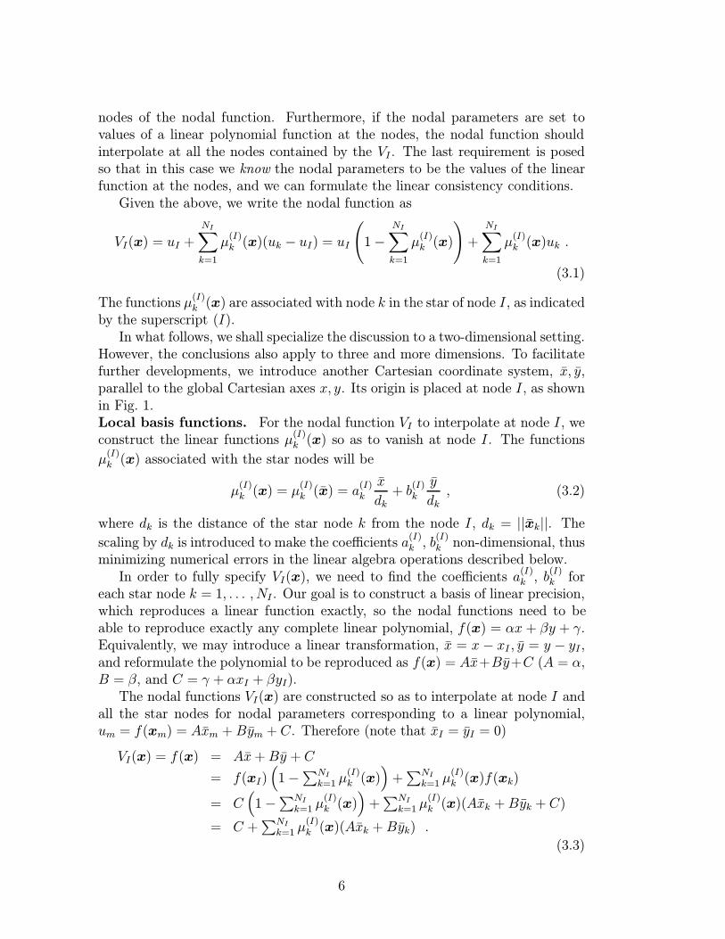
nodes of the nodal function. Furthermore, if the nodal parameters are set tovalues of a linear polynomial function at the nodes, the nodal function shouldinterpolate at all the nodes contained by the VI . The last requirement is posedso that in this case we know the nodal parameters to be the values of the linearfunction at the nodes, and we can formulate the linear consistency conditions.

Given the above, we write the nodal function as

VI(x) = uI +

NI∑k=1

µ(I)k (x)(uk − uI) = uI

(1−

NI∑k=1

µ(I)k (x)

)+

NI∑k=1

µ(I)k (x)uk .

(3.1)

The functions µ(I)k (x) are associated with node k in the star of node I, as indicated

by the superscript (I).In what follows, we shall specialize the discussion to a two-dimensional setting.

However, the conclusions also apply to three and more dimensions. To facilitatefurther developments, we introduce another Cartesian coordinate system, x, y,parallel to the global Cartesian axes x, y. Its origin is placed at node I, as shownin Fig. 1.Local basis functions. For the nodal function VI to interpolate at node I, weconstruct the linear functions µ(I)

k (x) so as to vanish at node I. The functions

µ(I)k (x) associated with the star nodes will be

µ(I)k (x) = µ

(I)k (x) = a

(I)k

x

dk+ b

(I)k

y

dk, (3.2)

where dk is the distance of the star node k from the node I, dk = ||xk||. The

scaling by dk is introduced to make the coefficients a(I)k , b

(I)k non-dimensional, thus

minimizing numerical errors in the linear algebra operations described below.In order to fully specify VI(x), we need to find the coefficients a

(I)k , b

(I)k for

each star node k = 1, . . . , NI . Our goal is to construct a basis of linear precision,which reproduces a linear function exactly, so the nodal functions need to beable to reproduce exactly any complete linear polynomial, f(x) = αx + βy + γ.Equivalently, we may introduce a linear transformation, x = x − xI , y = y − yI ,and reformulate the polynomial to be reproduced as f(x) = Ax+By+C (A = α,B = β, and C = γ + αxI + βyI).

The nodal functions VI(x) are constructed so as to interpolate at node I andall the star nodes for nodal parameters corresponding to a linear polynomial,um = f(xm) = Axm +Bym + C. Therefore (note that xI = yI = 0)

VI(x) = f(x) = Ax+By + C

= f(xI)(

1−∑NI

k=1 µ(I)k (x)

)+∑NI

k=1 µ(I)k (x)f(xk)

= C(

1−∑NI

k=1 µ(I)k (x)

)+∑NI

k=1 µ(I)k (x)(Axk +Byk + C)

= C +∑NI

k=1 µ(I)k (x)(Axk +Byk) .

(3.3)

6

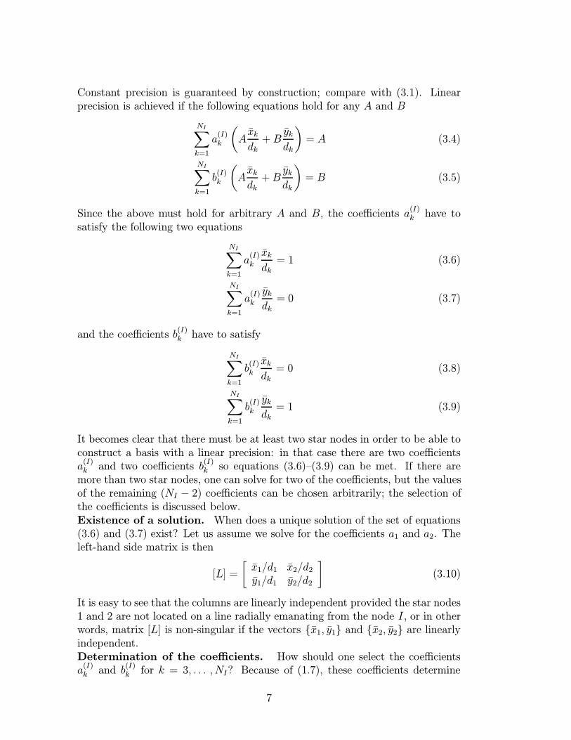
Constant precision is guaranteed by construction; compare with (3.1). Linearprecision is achieved if the following equations hold for any A and B

NI∑k=1

a(I)k

(Axkdk

+Bykdk

)= A (3.4)

NI∑k=1

b(I)k

(Axkdk

+Bykdk

)= B (3.5)

Since the above must hold for arbitrary A and B, the coefficients a(I)k have to

satisfy the following two equations

NI∑k=1

a(I)k

xkdk

= 1 (3.6)

NI∑k=1

a(I)k

ykdk

= 0 (3.7)

and the coefficients b(I)k have to satisfy

NI∑k=1

b(I)k

xk

dk= 0 (3.8)

NI∑k=1

b(I)k

ykdk

= 1 (3.9)

It becomes clear that there must be at least two star nodes in order to be able toconstruct a basis with a linear precision: in that case there are two coefficientsa

(I)k and two coefficients b

(I)k so equations (3.6)–(3.9) can be met. If there are

more than two star nodes, one can solve for two of the coefficients, but the valuesof the remaining (NI − 2) coefficients can be chosen arbitrarily; the selection ofthe coefficients is discussed below.Existence of a solution. When does a unique solution of the set of equations(3.6) and (3.7) exist? Let us assume we solve for the coefficients a1 and a2. Theleft-hand side matrix is then

[L] =

[x1/d1 x2/d2

y1/d1 y2/d2

](3.10)

It is easy to see that the columns are linearly independent provided the star nodes1 and 2 are not located on a line radially emanating from the node I, or in otherwords, matrix [L] is non-singular if the vectors x1, y1 and x2, y2 are linearlyindependent.Determination of the coefficients. How should one select the coefficientsa

(I)k and b

(I)k for k = 3, . . . , NI? Because of (1.7), these coefficients determine

7

the slope of the approximated function at the nodes. The question is then, howshould the coefficients a

(I)k be distributed to achieve a good approximation to the

derivatives of a given function at the node I? (Analogous reasoning applies to

the determination of the coefficients b(I)k .)

It is reasonable to require some kind of symmetry of the distribution withrespect to the axes x, y. Also, for a perfectly symmetric distribution of nodesthe coefficients should be also symmetric. For instance, for the star nodes ofFig. 2, both distributions of the coefficients a

(I)k , k = 0, . . . , 7 are acceptable. The

left side in fact loosely corresponds to a central difference estimate of the firstderivative with respect to x at the central node. One can expect a connectionbetween the design of the nodal function in the present method and the finitedifference approximations of derivative data. In particular, the connection to thegeneralized finite difference method of Liszka and Orkisz 17 seems worth exploring.

We propose the following rule for the initial selection of the coefficients a(I)k

for any irregular distribution of the star nodes (analogous estimates apply to the

coefficients b(I)k )

a(I)k =

(NI∑m=1

x2m

d2m

)−1

xkdk

. (3.11)

As can be easily verified, for symmetric arrangements of the star nodes, (3.11)satisfies (3.6) by construction. If either one of equations (3.6) and (3.7) is not

satisfied exactly for the values estimated from (3.11), the values of a(I)1 and a

(I)2

are obtained via the solution of (3.6) and (3.7).Some comments are in order: (i) one can expect deterioration of the absolute

accuracy for non-optimal distributions of the coefficients, but the convergencerate is not affected, since the linear precision conditions are met, (ii) further in-vestigation is needed to determine if there are optimality criteria for the selectionof the stars and for the distribution of the coefficients in the stars.Implementation. Applying the above results, equation (2.1) can be writtenas

uh(x) =N∑I=1

ωI(x)

[uI

(1−

NI∑k=1

µ(I)k (x)

)+

NI∑k=1

µ(I)k (x)uk

], (3.12)

which can be also converted to the standard form

uh(x) =N∑I=1

ϕI(x)uI , (3.13)

where the resulting linear-precision basis functions ϕI(x) are expressed as

ϕI(x) = ωI(x)

(1−

NI∑k=1

µ(I)k (x)

)+

AI∑k=1

ωk(x)µ(k)I (x) . (3.14)

8

Note the distinction in the sums: AI is the number of stars in which the node Iparticipates.

4 Numerical examples

In order to gain some insight into the properties of the proposed approximationbasis, we present L2 interpolation errors. The schemes compared are:

1. Moving least squares, which are used in the element-free Galerkin (EFG)method, with a linear basis11,13, 18,

2. FEM with linear triangles,

3. Interpolating PUM (the singular weight function of (1.5) is used),

4. Non-interpolating PUM (non-singular weight function of (1.8) is used).

Two surfaces have been approximated, S(x, y) = (−x3 + sin(2y) + xy/2)/4, andR(x, y) = −xy exp(−2x4y4); both on a square domain x ∈ 〈−2; 2〉2. Four gridshave been used. The spacing of the grids was set to 1/5, 1/10, 1/20 and 1/40of the length of the domain edge. An unstructured triangulation with edgesapproximately the same length was generated for each spacing, and the nodesin the meshless methods were placed at the vertices of the triangulation. (TheFEM solution was obtained on the triangulations, of course.) The support sizewas set to 1.7le for the meshless methods, EFG and the interpolating and non-interpolating PU; le is the average length of edges in the triangulation. TheEFG method used a linear basis, and a quartic polynomial weight function on aspherical support. For the EFG and the non-interpolating PU methods the nodalvalues were found from the interpolation conditions

[φI(xj)] fI = f(xj) (4.1)

The star nodes were selected from nodes within the domain of influence ofthe central node. As will be discussed later, the number of star nodes was eitherunlimited, or the nodes were sorted by distance, and only the closest to the centralnode have been considered.

The interpolation error is measured by the L2 norm

||f − fh||2L2=

∫[f(x)− fh(x)]2 dΩ , (4.2)

and error in derivatives is measured by the L2 seminorm

||∂f − ∂fh||2L2=

∫ [∂ f

∂ x(x)− ∂ fh

∂ x(x)

]2

+

[∂ f

∂ y(x)− ∂ fh

∂ y(x)

]2

dΩ , (4.3)

9

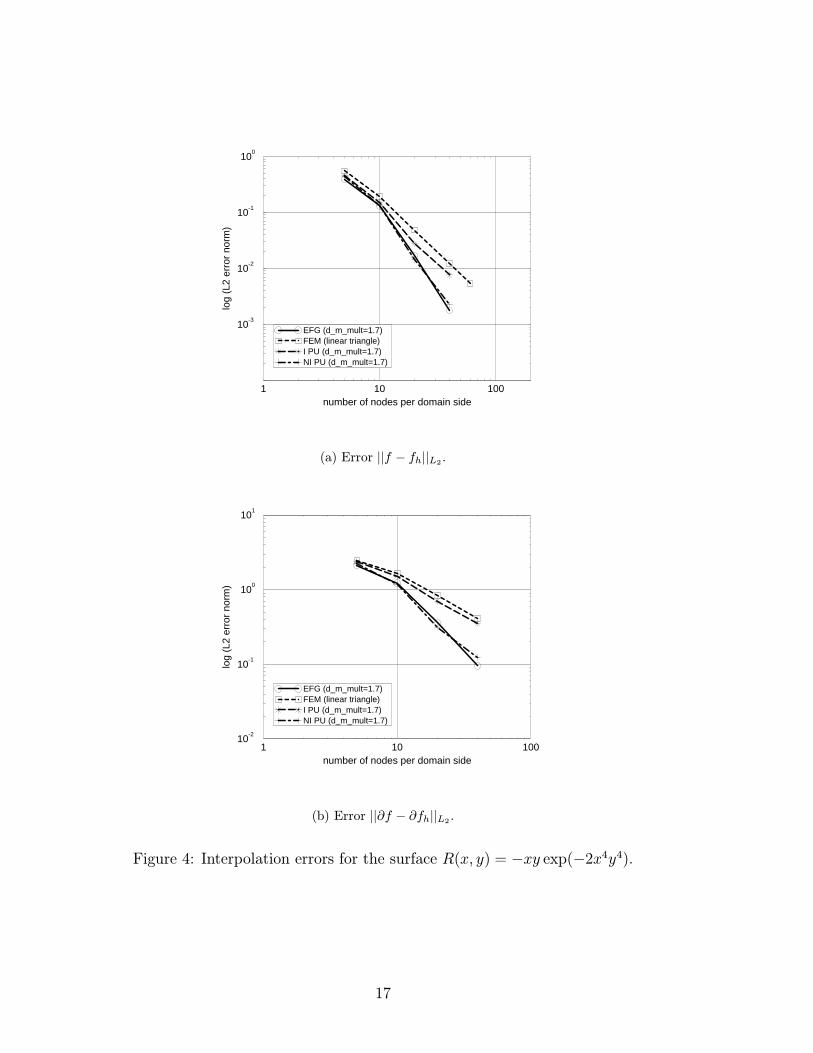
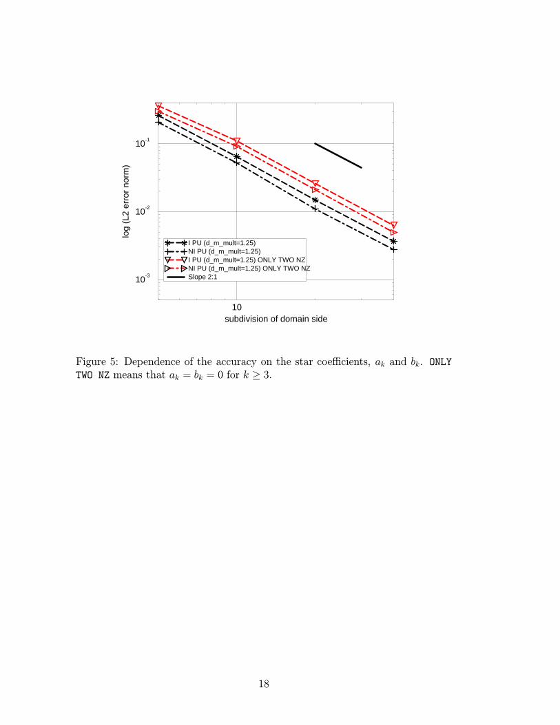
Figure 3 shows the convergence of the interpolation error norms for the surfaceS, and the corresponding interpolation errors for the surface R are shown inFig. 4. The expected convergence rate for linear triangles is two in the norm (4.2),and one in the norm (4.3). It can be seen that the EFG method and the non-interpolating PUM display similar absolute accuracy and convergence rates. Theinterpolating PUM is only slightly more accurate than the linear finite elements.The kink in Fig. 4 can be probably attributed to pre-asymptotic behavior, butthe convergence rate of the EFG and the present non-interpolating PUM is notcompletely understood yet.Dependence on the star coefficients In order to assess how the star coeffi-cients influence the accuracy we compare interpolation errors for the surface S forcoefficients obtained from (3.11), with results obtained for obviously non-optimalcoefficients ak = bk = 0, k ≥ 3. As can be seen from Fig. 5, the latter distributiongives slightly worse absolute accuracy, but the convergence rate is, as expected,unchanged.Dependence on the support size The support size, and in a related mannerthe number of star nodes selected at a given point, has a modest influence onthe absolute approximation errors. To assess this characteristic, we compare theinterpolation errors for varying support sizes. The support size is measured inmultiples of the smallest nodal spacing for a regular grid. The interpolation errorsare evaluated for the surface S on a perfectly regular grid of 10 × 10 nodes, andon a grid of 10× 10 nodes with slightly randomly shifted nodes (approx. 1/5 ofthe node spacing). Figure 6 shows the interpolation error for the case where allthe nodes inside the domain of influence of the center node are selected as starnodes; figure 7 depicts analogous results for the case the star nodes are limited tothe four closest nodes in the domain of influence of the center node. The accuracyof the present interpolating PUM is almost independent of the support size; theaccuracy of the non-interpolating PUM is comparable to the accuracy of the EFGmethod, but does not improve as markedly for larger supports. Interestingly, thepresent approach seems to be less sensitive to the irregularity of the grid thanthe EFG method.

5 Performance

The cost of the PU method of (2.1) is composed of the cost of constructingthe functions ωI(x) and of the cost involved in the computation of the nodalfunctions VI(x). Therefore, it is not possible to reduce the total CPU time costbelow that needed to construct the functions ωI(x). We use equation (1.2) toconstruct the functions ωI(x) (or, in other words, the Shepard approximation isused as the PU). In view of the preceding argument, we compare the cost of thepresented approach with the cost of the EFG method, and also with the cost ofthe evaluation of the PU functions ωI(x). The efficiency of the construction of thefunctions ωI(x) depends crucially on the efficiency with which nodes associated

10

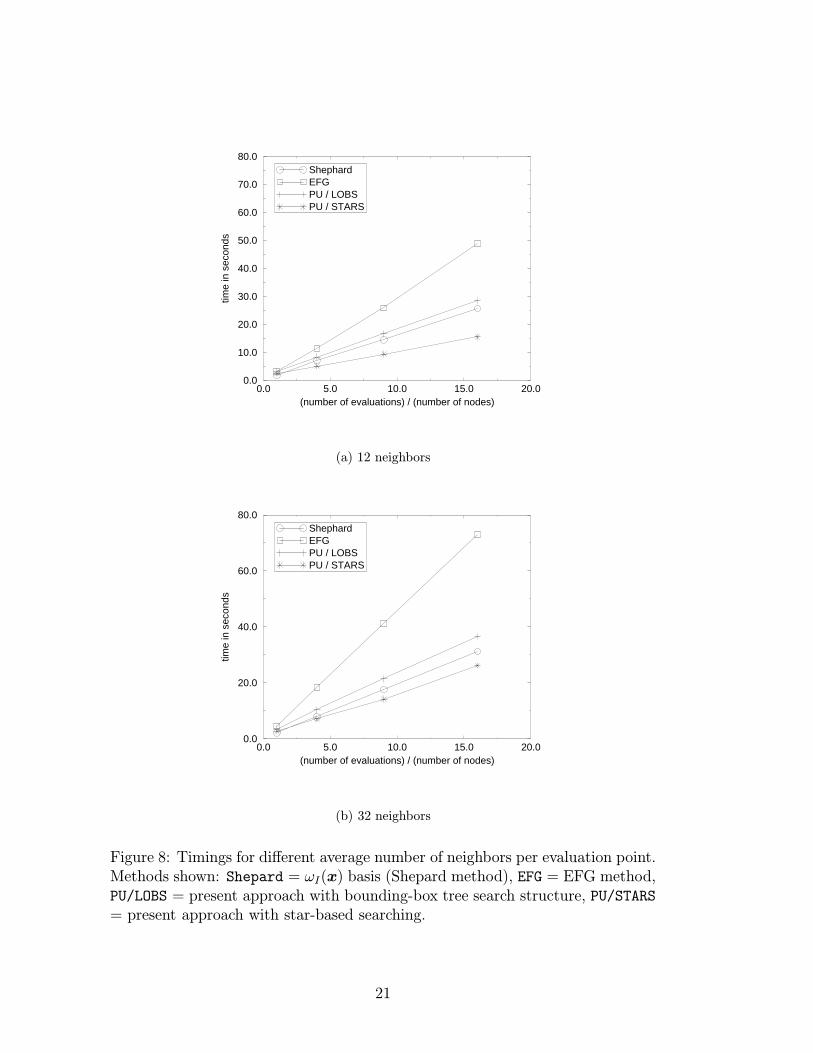
with non-zero weight can be found at any given point. We use a bounding-boxtree search technique with the EFG method.Star-based searching. Interestingly, the present approach allows us to use astar-based searching technique which is more efficient than the bounding-box treesearch. The star-based search makes use of the fact that one can search for onlya single node using the bounding-box tree search, and then the star connectivitycan be used to collect all the remaining nodes. (In order to make this work, allthe nodes in the domain of influence need to be included in the star.)Timing comparisons. We use a grid with 10,000 nodes, and we evaluatethe basis functions and their first derivatives at 10, 000×M randomly scatteredpoints, M = 1, 4, 9, 16. We measure the CPU time for the following methods: (i)Shepard method (or construction of the PU functions ωI(x)), (ii) EFG methodwith a linear basis, (iii) the present approach with a bounding-box tree searchstructure, (iv) the present approach with star-based searching.

The domains of influence of the nodes are square, and of two sizes leading to12 and 32 neighbors per evaluation point, respectively. The times are compared inFig. 8. As can be seen, the present approach using the bounding-box tree searchis only slightly slower than the construction of the PU functions ωI(x). Thisindicates that the effort expended in making the approximation basis linearlyprecise is minor, and in fact, the present method can be seen to be close tooptimal in the sense that the bulk of the cost is associated with the functionsωI(x).

As already mentioned, the connectivity information stored with the star ateach node allows us to use a more efficient way to construct the functions ωI(x),since the necessary searches can be performed more quickly. Therefore, thepresent method in conjunction with the more efficient searching technique is evenfaster than the construction of the functions ωI(x) using the slower bounding-boxtree searching method; compare with Fig. 8.

Conclusions

We have described how to construct approximation basis functions for a partition-of-unity (PU) method. The PU is in our case the Shepard basis. In order to en-hance its accuracy, we have designed linear-precision nodal functions (local fits)in such a way as to involve only the magnitude of the solution at the nodes asthe degrees of freedom. The nodal functions are sought as linear combinations ofthe nodal parameters at the central node and a set of near-by nodes, called thestar nodes. The unknown coefficients are computed in a pre-processing step. Theresulting approximation is meshless, and it is applicable to any number of spatialdimensions. Two variants can be constructed depending on the weight functionswhich generate the PU: an interpolating PU method (for singular weight func-tions), and a non-interpolating PU method. The non-interpolating PU methodis comparable in accuracy with the element free Galerkin (moving least squares)

11

method. The present method is very efficient, in fact the cost of the precisionenhancement constitutes only a small fraction of the cost involved in the con-struction of the Shepard basis. Furthermore, the connectivity information storedin the star allows for more efficient search. In this way the present linear-precisionbasis can be constructed with the more efficient search technique more quicklythan a constant-precision Shepard basis using the usual search strategy.

To summarize, the present approach has the following desirable properties:(i) the grid consists of scattered nodes, (ii) the basis exactly reproduces completelinear polynomials, (iii) only the values of the approximated function at the nodesare used as unknowns, (iv) the construction of the basis is only slightly moreexpensive than the Shepard constant-precision method, and, (v) the method isapplicable in any number of spatial dimensions.

Acknowledgments

The support of the Office of Naval Research is gratefully acknowledged. Theanonymous reviewers are thanked for useful comments.

References

[1] D. Shephard. A two dimensional interpolation function for irregularly spaceddata. In Proc. 23rd Nat. Conf. ACM, pages 517–523. ACM, 1968.

[2] D. H. McLain. Drawing contours from arbitrary data points. Comput. J.,17:318–324, 1974.

[3] D. H. McLain. Two-dimensional interpolation from random data. Comput.J., 19:178–181, 1976.

[4] R. Franke and G. Nielson. Smooth interpolation of large sets of scattereddata. International Journal of Numerical Methods in Engineering, 15:1691–1704, 1980.

[5] I. Babuska and J. M. Melenk. The partition of unity finite element method.Technical Report BN-1185, Institute for Physical Science and Technology,University of Maryland, 1995.

[6] I. Babuska and J. M. Melenk. The Partition of Unity Method. InternationalJournal of Numerical Methods in Engineering, 40:727–758, 1997.

[7] J. M. Melenk and I. Babuska. The Partition of Unity Method: Basic theoryand applications. Computer Methods in Applied Mechanics and Engineering,139:289–314, 1996.

12

[8] C. A. Duarte. A review of some meshless methods to solve partial differentialequations. Technical Report 95-06, Texas Institute for Computational andApplied Mathematics, University of Texas at Austin, 1995.

[9] C. A. Duarte and J. T. Oden. Hp clouds—a meshless method to solveboundary-value problems. Technical Report 95-05, Texas Institute for Com-putational and Applied Mathematics, University of Texas at Austin, 1995.

[10] C. A. Duarte and J. T. Oden. H-p clouds—an h-p meshless method. Nu-merical Methods for Partial Differential Equations, pages 1–34, 1996.

[11] T. Belytschko, Y.Y. Lu, and L. Gu. Element free Galerkin methods. Inter-national Journal for Numerical Methods in Engineering, 37:229–256, 1994.

[12] G. Strang and G. Fix. An Analysis of the Finite Element Method. Prentice-Hall, Englewood Cliffs, N.J., 1973.

[13] T. Belytschko, Y. Krongauz, D. Organ, M. Fleming, and P. Krysl. Mesh-less methods: An overview and recent developments. Computer Methods inApplied Mechanics and Engineering, 139:3–47, 1996.

[14] W. J. Gordon and J. A. Wixom. Shephard’s method of metric interpolationto bivariate and multivariate data. Math. Comput., 32:253–264, 1978.

[15] R. Franke. Scattered data interpolation: Test of some methods. Mathematicsof Computation, 38:181–200, 1982.

[16] N. Perrone and R. Kao. A general finite difference method for arbitrarymeshes. Computers and Structures, 5:45–47, 1975.

[17] T. Liszka and J. Orkisz. The finite difference method for arbitrary irregularmeshes — a variational approach to applied mechanics problems. GAMNI,pages 227–235, 1980.

[18] P. Krysl and T. Belytschko. ESFLIB: A library to compute the elementfree Galerkin shape functions. Computer Methods in Applied Mechanics andEngineering, 1998, to appear.

13

domain of influence

Ix

0

2

4

y3

1y

x

... star node of node I

Figure 1: The nodes constituting the star of node I, with the coordinate systemx, y.

.

14

a=0

x

y

I

x

y

0 1

2

3

4 5

6 7

domain of influenceof node I

d dx

y

I

x

y

0 1

2

3

4 5

6 7

domain of influenceof node I

d d

a=-1/8 a=1/8

a=1/4

a=-1/8 a=1/8

a=-1/4

a=0

a=-1/2 a=1/2

a=0

a=0a=0

a=0

a=0a=0

Figure 2: Regular arrangment of nodes.

15

1 10 100number of nodes per domain side

10-3

10-2

10-1

100

log

(L2

erro

r no

rm)

EFG (d_m_mult=1.7)FEM (linear triangle)I PU (d_m_mult=1.7)NI PU (d_m_mult=1.7)

(a) Error ||f − fh||L2 .


10-2

10-1

100

101

log

(L2

erro

r no

rm)


(b) Error ||∂f − ∂fh||L2 .

Figure 3: Interpolation errors for the surface S(x, y) = (−x3 + sin(2y) +xy/2)/4.

16


10-3

10-2

10-1

100

log

(L2

erro

r no

rm)


(a) Error ||f − fh||L2 .


10-2

10-1

100

101

log

(L2

erro

r no

rm)


(b) Error ||∂f − ∂fh||L2 .

Figure 4: Interpolation errors for the surface R(x, y) = −xy exp(−2x4y4).

17

10subdivision of domain side

10-3

10-2

10-1

log

(L2

erro

r no

rm)

I PU (d_m_mult=1.25)NI PU (d_m_mult=1.25)I PU (d_m_mult=1.25) ONLY TWO NZNI PU (d_m_mult=1.25) ONLY TWO NZSlope 2:1

Figure 5: Dependence of the accuracy on the star coefficients, ak and bk. ONLY

TWO NZ means that ak = bk = 0 for k ≥ 3.

18

1.0 2.0 3.0support size in multiples of node spacing

10-3

10-2

10-1

100

101

log(

L2 e

rror

nor

m)

EFGPUIPUNI

(a) Regular grid


10-3

10-2

10-1

100

101

log(

L2 e

rror

nor

m)

EFGPUIPUNI

(b) Irregular grid

Figure 6: Interpolation errors ||f − fh||L2 for varying support size. Grid 10× 10nodes. Quartic circular weight. All the nodes inside the domain of influence ofthe center node are selected as the star nodes.

19


10-3

10-2

10-1

100

101

log(

L2 e

rror

nor

m)

EFGPUIPUNI

(a) Regular grid


10-3

10-2

10-1

100

101

log(

L2 e

rror

nor

m)

EFGPUIPUNI

(b) Irregular grid

Figure 7: Interpolation errors ||f − fh||L2 for varying support size. Grid 10× 10nodes. Quartic circular weight. Only the closest four nodes are selected as thestar nodes.

20

0.0 5.0 10.0 15.0 20.0(number of evaluations) / (number of nodes)

0.0

10.0

20.0

30.0

40.0

50.0

60.0

70.0

80.0

time

in s

econ

ds

ShephardEFGPU / LOBSPU / STARS

(a) 12 neighbors

0.0 5.0 10.0 15.0 20.0(number of evaluations) / (number of nodes)

0.0

20.0

40.0

60.0

80.0

time

in s

econ

ds

ShephardEFGPU / LOBSPU / STARS

(b) 32 neighbors

Figure 8: Timings for different average number of neighbors per evaluation point.Methods shown: Shepard = ωI(x) basis (Shepard method), EFG = EFG method,PU/LOBS = present approach with bounding-box tree search structure, PU/STARS= present approach with star-based searching.

21

Documents

An e cient linear-precision partition of unity basis for