A Particle-Partition of Unity Method{Part IV: Parallelizationwissrech.ins.uni-bonn.de/research/pub/schweitzer/... · · 2015-03-23A Particle-Partition of Unity Method{Part IV: Parallelization

A Particle-Partition of Unity Method–Part IV:Parallelization

Michael Griebel and Marc Alexander Schweitzer

Institut fur Angewandte Mathematik, Universitat Bonn, Bonn, Germany.

Abstract In this sequel to [7, 8, 9] we focus on the parallelization of our multilevelpartition of unity method for distributed memory computers. The presented par-allelization is based on a data decomposition approach which utilizes a key-basedtree implementation and a weighted space filling curve ordering scheme for the loadbalancing problem. We present numerical results with up to 128 processors. Theseresults show the optimal scaling behavior of our algorithm.

1 Introduction

Numerical simulations with millions of degrees of freedom require the useof optimal order algorithms. Here, the number of operations necessary toobtain an approximate solution within a given accuracy should be of the or-der O(dof). But still the overall computing time can be unacceptably large.Another problem with large simulations is their storage demand. These is-sues make the use of parallel computers with distributed memory a must forlarge numerical simulations. Here, the data have to be partitioned into al-most equally sized parts and assigned to different segments of the distributedmemory to exploit the available memory. This partitioning, however, shouldallow for a single processor to complete most operations on its assigned partof the data independently of the other processors. Furthermore, the numberof operations per processor should be almost identical to utilize all availableprocessors for the larger part of the computation.

In this paper we present the parallelization of our multilevel particle-partition of unity method for the approximate solution of an elliptic partialdifferential equation. The main ingredients are a key-based tree implemen-tation and a space filling curve load balancing scheme. The overall methodcan be split into three major steps: The initial tree construction and loadbalancing step, the assembly step where we set up the stiffness matrices Akand interlevel transfers on all levels k = 0, . . . , J , and finally the solutionstep where we use a multiplicative multilevel iteration to solve the linear(block-)system AJ uJ = fJ . The complexities of the tree construction andload balancing step is given by O(N℘ J + (N℘ )

d−1d + J(log℘)2 +℘ log℘) where

N denotes the number of leaves of the tree, J denotes the number of levels ofthe tree (J ' logN for a balanced tree) and ℘ is the number of processors.The assembly of the stiffness matrices is trivially parallel with a complexity

2 M. Griebel, M. A. Schweitzer

of O(N℘ ), and the complexity of the solution step is the well-known complex-

ity O(N℘ + (N℘ )d−1d + J + log℘) of a multiplicative multilevel iteration [26].

The results of our numerical experiments with up to 128 processors and 42million degrees of freedom clearly show the scalability of our method.

The remainder of the paper is organized as follows. In §2 we shortly re-view the Galerkin discretization and multilevel solution of an elliptic partialdifferential equation with the particle-partition of unity method. The paral-lelization of our method is presented in §3. Here, a fundamental ingredientis a key-based tree implementation which we introduce in §3.2 and §3.3. Wefocus on the load balancing problem in §3.4. There, we present a cheap nu-merical scheme based on space filling curves to (re-)partition data in parallel.The algorithmic changes we have to apply to our particle-partition of unityfor parallel computations are presented in §3.5, §3.6 and §3.7. The resultsof our numerical experiments are presented in §4. Finally, we conclude withsome remarks in §5.

2 Particle-Partition of Unity Method

In the following, we give a short recap of our particle-partition of unitymethod for the Galerkin discretization of an elliptic partial differential equa-tion of second order and its multilevel solution, see [7, 8, 9, 19] for details.

2.1 Construction of Partition of Unity Spaces

In a partition of unity method (PUM), we define a global approximation uPU

simply as a weighted sum of local approximations ui,

uPU(x) :=N∑i=1

ϕi(x)ui(x). (2.1)

These local approximations ui are completely independent of each other. Thelocal supports ωi := supp(ui), the local basis ψni and the order of approxi-mation pi for every single ui :=

∑n u

ni ψ

ni can be chosen independently of all

other uj . Here, the functions ϕi form a partition of unity (PU), i.e.∑i ϕi ≡ 1.

They are used to splice the local approximations ui together in such a waythat the global approximation uPU benefits from the local approximation or-ders pi, yet it still fulfills global regularity conditions. For further details see[7, 19].

The starting point for any meshfree method is a collection of N indepen-dent points P := xi ∈ Rd |xi ∈ Ω, i = 1, . . . , N. In the partition of unityapproach we first have to construct a PU ϕi on the domain of interestΩ. Then we can choose local approximation spaces V pii = span〈ψni 〉 on thepatches ωi to define the PUM space

V PU :=∑i

ϕiVpii =

∑i

ϕi span〈ψni 〉 = span〈ϕiψni 〉

A Particle-Partition of Unity Method–Part IV: Parallelization 3

and an approximate solution (2.1). Here, the union of the supports supp(ϕi) =ωi have to cover the domain, i.e. Ω ⊂

⋃Ni=1 ωi. Given a cover CΩ := ωi | i =

1, . . . , N we can define a PU by using Shepard functions as ϕi.The efficient construction of an appropriate cover CΩ for general point sets

P is not an easy task [7, 8, 19] and it is the most crucial step in a PUM. Thecover has a significant impact on the computational costs associated withthe assembly of the stiffness matrix A, since the cover already defines the(block-)sparsity pattern of the stiffness matrix, i.e. the number of integralsto be evaluated. Furthermore, the cover influences the algebraic structure ofthe PU functions ϕi, which has to be resolved for the proper integration ofa stiffness matrix entry [7, 8, 19]. Throughout this paper we use a parallelversion (see §3.5) of a tree-based algorithm for the construction of a sequenceof rectangular covers [8, 9].

With the help of weight functions Wk defined on the patches ωk of thecover CΩ we can easily generate a PU by Shepard’s method, i.e. we define

ϕi(x) =Wi(x)∑

ωk∈CiWk(x), (2.2)

where Ci := ωj ∈ CΩ |ωi ∩ωj 6= ∅ is the set of all geometric neighbors of acover patch ωi. We restrict ourselves to the use of cover patches ωi which ared-rectangular, i.e. the patches ωi are products of intervals [xli − hli, xli + hli].Therefore, the most natural choice for a weight function Wi is a product ofone-dimensional functions, i.e. Wi (x) =

∏dl=1W

li (xl) =

∏dl=1W (x

l−xli+hli

2hli)

with supp(W) = [0, 1] such that supp(Wi) = ωi. It is sufficient for thisconstruction to choose a one-dimensional weight function W which is non-negative. The PU functions ϕi inherit the regularity of the generating weightfunction W. We always use a normed B-spline [19] as the generating weightfunction W, throughout this paper we use a linear B-spline.

In general, a PU ϕi can only recover the constant function on the do-main Ω. For the discretization of a partial differential equation (PDE) this ap-proximation quality is not sufficient. Therefore, we multiply the PU functionsϕi locally with polynomials ψni . Since our cover patches ωi are d-rectangular, alocal tensor product space is the most natural choice. Throughout this paper,we use products of univariate Legendre polynomials as local approximationspaces V pii , i.e. we choose

V pii = span〈ψni |ψni =d∏l=1

Lnli , ‖n‖1 =d∑l=1

nl ≤ pi〉,

where n = (nl)dl=1 is the multi-index of the polynomial degrees nl of theunivariate Legendre polynomials Lnli : [xli − hli, xli + hli] → R, and n is theindex associated with the product function ψni =

∏dl=1 L

nli .


2.2 Galerkin Discretization

We want to solve elliptic boundary value problems of the type

Lu = f in Ω ⊂ Rd ,Bu = g on ∂Ω ,

where L is a symmetric partial differential operator of second order and Bexpresses suitable boundary conditions. For reasons of simplicity we considerin the following the model problem

−∆u+ u = f in Ω ⊂ Rd ,∇u · nΩ = g on ∂Ω ,

(2.3)

of Helmholtz type with natural boundary conditions. The Galerkin discretiza-tion of (2.3) leads to a definite linear system.1 In the following let a (·, ·) bethe continuous and elliptic bilinear form induced by L on H1(Ω). We dis-cretize the PDE using Galerkin’s method. Then, we have to compute thestiffness matrix

A = (A(i,n),(j,m)) , with A(i,n),(j,m) = a (ϕjψmj , ϕiψni ) ∈ R ,

and the right hand side vector

f = (f(i,n)) , with f(i,n) = 〈f, ϕiψni 〉L2 =∫Ω

fϕiψni ∈ R .

Throughout this paper we assume that the stiffness matrix is arranged inpolynomial blocks Ai,j = (A(i,n),(j,m)) [9].

The integrands of the weak form of (2.3) may have quite a number ofjumps of significant size since we use piecewise polynomial weights Wi whosesupports ωi overlap in the Shepard construction (2.2). Therefore, the inte-grals of the weak form have to be computed carefully using an appropriatenumerical quadrature scheme, see [7, 8].

2.3 Multilevel Solution

We use a multilevel solver developed in [9] for the fast and efficient solutionof the resulting large sparse linear (block-)system Au = f , where u denotesa coefficient (block-)vector and f a moment (block-)vector.1 The implementation of Neumann boundary conditions with our PUM is straight-

forward and similar to their treatment within the finite element method (FEM).The realization of essential boundary conditions with meshfree methods is moreinvolved than with a FEM due to the non-interpolatory character of the meshfreeshape functions. There are several different approaches to the implementation ofessential boundary conditions with meshfree approximations, see [1, 7, 12, 19].Note that the resulting linear system may be indefinite, e.g. when we use La-grangian multipliers to enforce the essential boundary conditions. A more naturalapproach toward the treatment of Dirichlet boundary conditions due to Nitsche[16] leads to a definite linear system.


In a multilevel method we need a sequence of discretization spaces Vkwith k = 0, . . . , J where J denotes the finest level. To this end we constructa sequence of PUM spaces V PU

k as follows. We use a tree-based algorithmdeveloped in [8, 9] to generate a sequence of point sets Pk and covers CkΩfrom a given initial point set P . Following the construction given in §2.1 wecan then define an associated sequence of PUM spaces V PU

k . Note that thesespaces are nonnested, i.e. V PU

k−1 6⊂ V PUk , and that the shape functions ϕi,kψni,k

are non-interpolatory. Thus, we need to construct appropriate transfer op-erators Ikk−1 : V PU

k−1 → V PUk and Ik−1

k : V PUk → V PU

k−1. With such transferoperators Ikk−1, Ik−1

k and the stiffness matrices Ak coming from the Galerkindiscretization on each level k we can then set up a standard multiplicativemultilevel iteration to solve the linear system AJ uJ = fJ .

Our multilevel solver utilizes special localized L2-projections for the in-terlevel transfers and a block-smoother to treat all local degrees of freedomψni within a patch ωi simultaneously. For further details see [9].

3 Parallel Particle-Partition of Unity Method

In this section we present the parallelization of our PUM. Here, we use adata decomposition approach to split up the data among the participatingprocessors and their respective local memory.

Our cover construction algorithm [8] is essentially a simple tree algorithm.Hence, we need to be concerned with a parallel tree implementation (§3.2and §3.3). Another cause of concern in parallel computations is the loadbalancing issue which we discuss in §3.4. We then focus on the parallel coverconstruction in §3.5 where we construct a sequence of d-rectangular coversCkΩ . The assembly of the stiffness matrices Ak on all levels k in parallel ispresented in §3.6. Finally, we discuss the multilevel solution of AJ uJ = fJ inparallel in §3.7.

Note that neither the assembly phase nor the solution phase make explicituse of the tree data structure. Here, we employ a parallel sparse matrix datastructure to store each of the sparse (block-)matrices Ak, Ikk−1 and Ik−1

k on alllevels k. The neighborhoods Ci,k := ωj,k ∈ CkΩ |ωj,k ∩ ωi,k 6= ∅ determinethe sparsity pattern of the stiffness matrices Ak, i.e. the nonzero (block-)-entries of the ith (block-)row. Furthermore, they are needed for the evaluationof (2.2). Once the neighborhoods are known the evaluation of a PU function(2.2) and the matrix assembly are independent of the tree construction. Thetree data structure is used only for the multilevel cover construction and forthe efficient computation of the neighborhoods Ci,k.

3.1 Data Decomposition

There are two main tasks associated with the efficient parallelization of anynumerical computation on distributed memory computers. The first is to


evenly split up the data among the participating processors, i.e. the asso-ciated computational work should be well-balanced. The second is to allowfor an efficient access to data stored by another processor; i.e. on distributedmemory parallel computers also the amount of remote data needed by aprocessor should be small.

In a data decomposition approach we partition the data, e.g. the compu-tational domain or mesh, among the participating processors [17]. Then, wesimply restrict the operations of the global numerical method to the assignedpart of the data/domain. A processor has read and write access to its localdata but only read access to remote data it may need to complete its localcomputation. On distributed memory machines these required data have beto exchanged explicitly in distinct communication steps.

The quality of the partition of the domain/data essentially determinesthe efficiency of the resulting parallel computation. The local parts of thedata assigned to each processor should induce a similar amount of computa-tional work so that each processor needs roughly the same time to completeits local computation. Here, a processor may need to access the data of theneighboring sub-domains to solve its local problem. Hence, the geometry ofthe sub-domains should be simple to limit the number of communicationsteps and the communication volume. The number of neighboring processors(which determines the number of communication steps) should be small andthe geometry of the local boundary (which strongly influences the communi-cation volume) should be simple, i.e. its size should be small.

The data structure which describes the computational domain in ourPUM is a d-binary tree (quadtree, octree) used for the cover construction[8] and the fast neighbor search for the evaluation of the Shepard PU func-tions (2.2). In a conventional implementation of a d-binary tree the topologyis represented by storing links to the successor cells in the tree cells. Notethat this data structure does not allow for random access to a particular cellof the tree and special care has to be taken on distributed memory machinesif a successor cell is assigned to another processor. These issues make the useof a conventional tree implementation rather cumbersome on a distributedmemory parallel computer.

3.2 Key Based Tree Implementation

A different implementation of a d-binary tree which is more appropriate fordistributed memory machines was developed in [23, 24]. Here, the tree isrealized with the help of a hashed associative container. A unique label isassigned to each possible tree cell and instead of linking a cell directly to itssuccessor cells the labeling scheme implicitly defines the topology of the treeand allows for the easy access to successors and ancestors of a particular treecell. Furthermore, we can randomly access any cell of the tree via its uniquelabel. This allows us to catch accesses to non-local data and we can easily


compute the communication pattern and send and receive all necessary datato complete the local computation.

The labeling scheme maps tree cells CL =⊗d

i=1[ciL, ciL + hiL] ⊂ Rd to a

single integer value kL ∈ N0, the key. For instance, we can use the d-binarypath as the key value kL associated with a tree cell CL. The d-binary path kLis defined by the search path that has to be completed to find the respectivecell in the tree. Starting at the root of the tree we set kL = 1 and descendthe tree in the direction of the cell CL. Here we concatenate the current keyvalue (in binary representation) and the d Boolean values 0 and 1 associatedwith the decisions to which successor cell the descent continues to reach therespective tree cell CL. In Table 1 we give the resulting path key values kLfor a two dimensional example. Note that the key value kL = 1 for the rootcell is essentially a stop bit which is necessary to insure the uniqueness of thekey values.

Table1. Path key values for the successor cells of a tree cell CL =⊗di=1[ciL, c

iL + hiL] with associated key kL in two dimensions.

successor cell binary key value integer key value

[c1L, c1L + 1

2h1L] × [c2L, c

2L + 1

2h2L] kL00 4kL

[c1L, c1L + 1

2h1L] × [c2L + 1

2h2L, c

2L + h2

L] kL01 4kL + 1

[c1L + 12h1L, c

1L + h1

L] × [c2L, c2L + 1

2h2L] kL10 4kL + 2

[c1L + 12h1L, c

1L + h1

L] × [c2L + 12h2L, c

2L + h2

L] kL11 4kL + 3

3.3 Parallel Key Based Tree Implementation

The use of a global unique integer key for each cell of the tree allows for asimple description of a partitioning of the computational domain. The set ofall possible2 keys 0, 1, . . . , kmax is simply split into ℘ subsets which are thenassigned to the ℘ processors. We subdivide the range of keys into ℘ intervals

0 = r0 ≤ r1 ≤ · · · ≤ r℘ = kmax

and assign the interval [rq, rq+1) to the qth processor, i.e. the set of treecells assigned to the qth processor is CL | kL ∈ [rq, rq+1). With this verysimple decomposition each processor can identify which processor stores aparticular tree cell CL. A processor only has to compute the key value kL forthe tree cell CL and the respective interval [rq, rq+1) with kL ∈ [rq, rq+1) todetermine the processor q which stores this tree cell CL. The question nowarises if such a partition of the domain with the path keys kL is a reasonable2 The maximal key value kmax is a constant depending on the architecture of the

parallel computer.


k=4

k=1

k=5 k=6 k=7

k=23k=22k=21k=20

Figure1. The tree is ordered horizontally by the path key values k.

choice? Obviously the partitioning of the tree should be done in such a fashionthat complete sub-trees are assigned to a processor to allow for efficient treetraversals. But the path key labeling scheme given above orders the tree cellsrather horizontally (see Figure 1) instead of vertically. Therefore, we need totransform the path keys kL to so-called domain keys kDL .

A simple transformation which leads to a vertical ordering of the tree cellsis the following: First, we remove the leading bit (the initial root key value)from the key’s binary representation. Then we shift the remaining bits all theway to the left so that the leading bit of the path information is now storedin the most significant bit.3 Assume that the key values are stored as an 8 bitinteger and that we are in two dimensions. Then this simple transformationof a path key value kL = 18 to a respective domain key value kDL = 32 isgiven by

kL = 0001 0010︸︷︷︸path

7→ 0010︸︷︷︸path

0000 = kDL . (3.1)

With these domain keys kDL the tree is now ordered vertically and we canassign complete sub-trees to a processor using the simple interval domaindescription [rq, rq+1). But the transformed keys are no longer unique andcannot be used as the key value for the associative container to store thetree itself. Obviously, a successor cell CS of a tree cell CL can be assigned thesame domain key as the tree cell, i.e. kDS = kDL . Hence, we use the uniquepath keys kL for the container and the associated domain keys kDL for thedomain description, i.e. for the associated interval boundaries [rq, rq+1).

Note that the description of the data partition via the intervals [rq, rq+1)defines a minimal refinement stage of the tree which has to be present on allprocessors to insure the consistency of the tree. In the following we refer tothis top part of the tree as the common global tree. The leaves CL of the com-mon global tree are characterized by the fact that they are the coarsest treecells for which all possible successor cells are stored on the same processor,see Figure 2. The domain key values kDS of all possible successor cells CS lie

3 This transformation needs O(1) operations if we assume that the current refine-ment level of the tree is known, otherwise it is of the order O(J), where J denotesthe number of levels of the tree.


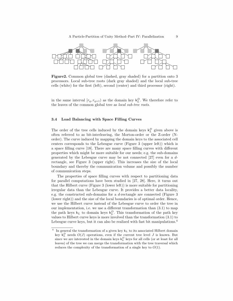
Figure2. Common global tree (dashed, gray shaded) for a partition onto 3processors. Local sub-tree roots (dark gray shaded) and the local sub-treecells (white) for the first (left), second (center) and third processor (right).

in the same interval [rq, rq+1) as the domain key kDL . We therefore refer tothe leaves of the common global tree as local sub-tree roots.

3.4 Load Balancing with Space Filling Curves

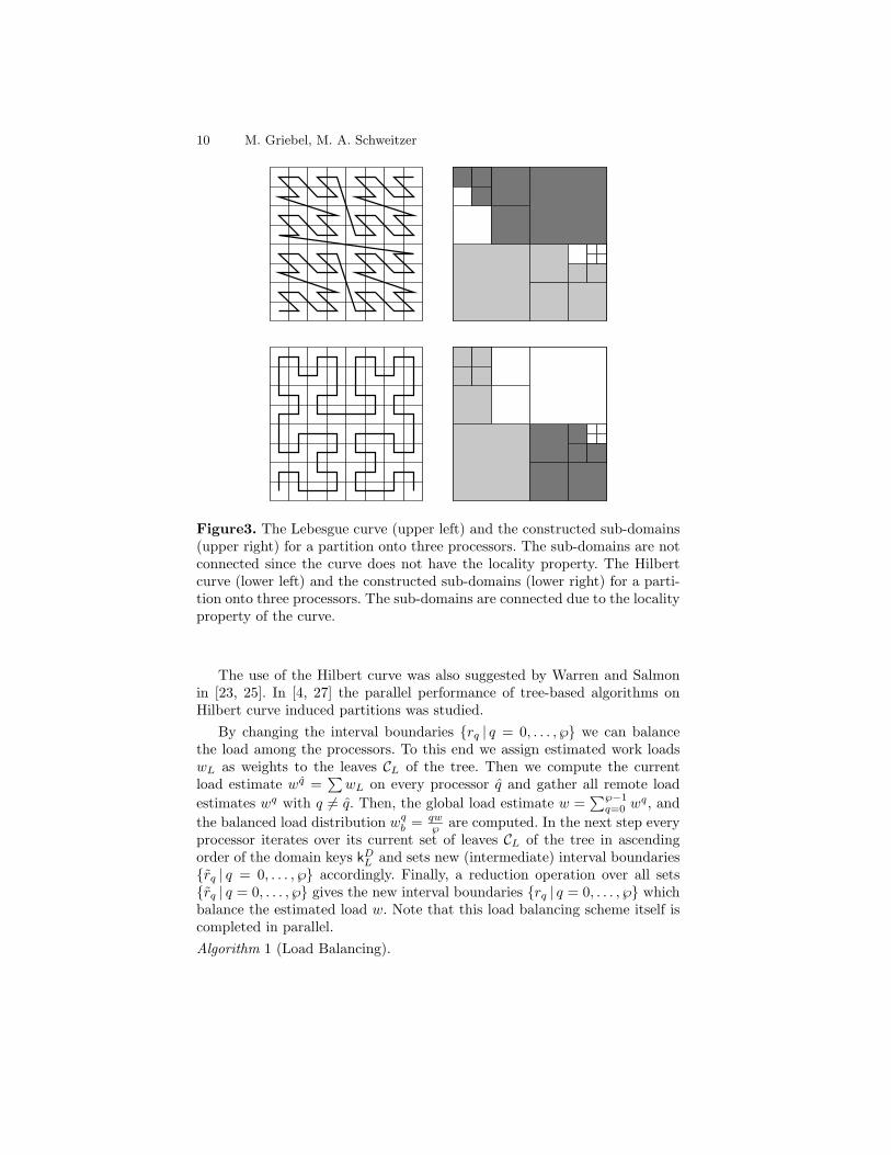
The order of the tree cells induced by the domain keys kDL given above isoften referred to as bit-interleaving, the Morton-order or the Z-order (N-order). The curve induced by mapping the domain keys to the associated cellcenters corresponds to the Lebesgue curve (Figure 3 (upper left)) which isa space filling curve [18]. There are many space filling curves with differentproperties which might be more suitable for our needs; e.g. the sub-domainsgenerated by the Lebesgue curve may be not connected [27] even for a d-rectangle, see Figure 3 (upper right). This increases the size of the localboundary and thereby the communication volume and possibly the numberof communication steps.

The properties of space filling curves with respect to partitioning datafor parallel computations have been studied in [27, 28]. Here, it turns outthat the Hilbert curve (Figure 3 (lower left)) is more suitable for partitioningirregular data than the Lebesgue curve. It provides a better data locality,e.g. the constructed sub-domains for a d-rectangle are connected (Figure 3(lower right)) and the size of the local boundaries is of optimal order. Hence,we use the Hilbert curve instead of the Lebesgue curve to order the tree inour implementation, i.e. we use a different transformation than (3.1) to mapthe path keys kL to domain keys kDL . This transformation of the path keyvalues to Hilbert curve keys is more involved than the transformation (3.1) toLebesgue curve keys, but it can also be realized with fast bit manipulations.4

4 In general the transformation of a given key kL to its associated Hilbert domainkey kDL needs O(J) operations, even if the current tree level J is known. Butsince we are interested in the domain keys kDL keys for all cells (or at least for allleaves) of the tree we can merge the transformation with the tree traversal whichreduces the complexity of the transformation of a single key to O(1).


Figure3. The Lebesgue curve (upper left) and the constructed sub-domains(upper right) for a partition onto three processors. The sub-domains are notconnected since the curve does not have the locality property. The Hilbertcurve (lower left) and the constructed sub-domains (lower right) for a parti-tion onto three processors. The sub-domains are connected due to the localityproperty of the curve.

The use of the Hilbert curve was also suggested by Warren and Salmonin [23, 25]. In [4, 27] the parallel performance of tree-based algorithms onHilbert curve induced partitions was studied.

By changing the interval boundaries rq | q = 0, . . . , ℘ we can balancethe load among the processors. To this end we assign estimated work loadswL as weights to the leaves CL of the tree. Then we compute the currentload estimate wq =

∑wL on every processor q and gather all remote load

estimates wq with q 6= q. Then, the global load estimate w =∑℘−1q=0 w

q, andthe balanced load distribution wqb = qw

℘ are computed. In the next step everyprocessor iterates over its current set of leaves CL of the tree in ascendingorder of the domain keys kDL and sets new (intermediate) interval boundariesrq | q = 0, . . . , ℘ accordingly. Finally, a reduction operation over all setsrq | q = 0, . . . , ℘ gives the new interval boundaries rq | q = 0, . . . , ℘ whichbalance the estimated load w. Note that this load balancing scheme itself iscompleted in parallel.Algorithm 1 (Load Balancing).


1. For all local leaves CL of the tree: Assign estimated work load wL.2. Compute local estimate wq =

∑L wL.

3. Gather remote estimates wq with q = 0, . . . , ℘− 1 and q 6= q.4. Compute global load estimate w =

∑℘−1q=0 w

q.

5. Set local estimate wqg =∑q<qq=0 w

q.6. Set balanced load distribution wqb = qw

℘ for q = 0, . . . , ℘.7. For all local leaves CL (in ascending order of domain keys kDL ): Set local

intermediate interval boundary rq = kDL where q ∈ 0, . . . , ℘ is thesmallest integer with wqg ≤ w

qb and update estimate wqg = wqg + wL.

8. Set interval boundaries rq = maxq rq by reducing the intermediate bound-aries rq over all processors, force r0 = 0 and r℘ = kmax.

The complexity of this load balancing scheme is given by O( card(PJ )℘ +

℘ log℘), where PJ denotes the generating point set for our PUM space V PUJ

on the finest level J , i.e. card(PJ) corresponds to the number of leaves ofthe tree.5 We use the number of neighboring patches card(CL,J) on the finestlevel J as the load work estimate wL. By this choice we balance the number of(block-)integrals on the finest level among the processors. Under the assump-tion that the computation of every (block-)integral is equally expensive webalance the assembly of the operator on level J . Since we use a dynamic inte-gration scheme [8] this assumption does not hold exactly but our experimentsindicate that the difference in the cost of the integration is small. A slightlybetter load balance might be achieved if we use the number of integrationcells [8] per (block-)row instead of the number of (block-)entries, but still thenumber of quadrature points may not be balanced. Furthermore, the maininfluence on the number of quadrature cells is the number of neighboringpatches [8].

Currently, our load estimator wL involves only the neighbors CL,J on thefinest level J . But for highly irregular point sets we might need to includean estimate of the computational work on coarser levels as well. To this endwe could either include the number of neighbors card(CL,k) on coarser levelsk < J or take the local refinement level of the tree into account. Furthermore,the estimator does not involve the local polynomial degrees pi which influencethe cost during the integration. In applications with a large variation of thelocal polynomial degrees pi or varying local basis functions ψni the estimatorshould also take these features into account.

Note that the computational cost associated with the estimation of thecurrent load can often be reduced. In a time-dependent setting or in adaptiverefinement we usually have a pretty good load estimate from a previous timestep or a coarser level without extra computations. This estimate can eitherbe used directly to partition the data or it can be updated with only a

5 The complexity may be reduced to O( card(PJ )℘

+log℘) only under very restrictiveassumptions on the load imbalance.


few operations. Furthermore, we typically have to re-distribute only a smallamount of data in these situations.

Let us now consider the solution phase of our PUM where we use ourmultilevel iteration to solve the linear (block-)system AJ uJ = fJ . The solveressentially consist of matrix-vector-products and scalar-products. So we needto be concerned with the performance of these two basic operations.

Our load balancing strategy partitions the number of (block-)integralsevenly among the processors so that we have an optimal load balance inthe assembly of the stiffness matrix. Hence, the number of (block-)entries inthe stiffness matrix AJ per processor are also (almost) identical due to thisbalancing strategy, i.e. the number of operations in a matrix-vector-productis balanced among the processors. Unlike in grid-based discretizations wehave to cope with a varying “stencil size”, i.e. the number of (block-)entriesper (block-)row in the stiffness matrix is not constant. Therefore, the perfectload balance for the matrix-vector-product does no longer coincide with theload balance for the scalar-product. Since a matrix-vector-product is certainlymore expensive than a scalar-product the parallel performance of the overalliteration is dominated by the performance of the matrix-vector-product wherewe have a perfect load balance. Hence, our balancing scheme leads to anoptimal load balance in the discretization phase as well as in the solutionphase.

3.5 Parallel Cover Construction

Now that the computational domain is partitioned in an appropriate fashionamong the processors we turn to the algorithmic changes for our parallelimplementation, e.g. the computation of the communication pattern. Thefirst task in our PUM is the multilevel cover construction [8, 9] which isessentially a post-order tree operation. Due to our tree decomposition whichassigns complete sub-trees to processors most work can be done completelyin parallel. When we reach elements of the common global tree we need togather the respective tree cells from remote processors. Then, all processorscan complete the cover construction on the common global tree. The parallelversion of the multilevel cover construction algorithm [8, 9] reads as:Algorithm 2 (Parallel Multilevel Cover Construction).

1. Given the domain Ω ⊂ Rd and a bounding box RΩ =⊗d

i=1[liΩ , uiΩ ] ⊃ Ω.

2. Given the interval boundaries rq | q = 0, . . . , ℘ and the local part Pqof the initial point set P = xj |xj ∈ Ω, i.e. kDj ∈ [rq, rq+1) for allxj ∈ Pq.6

3. Initialize the common global d-binary tree (quadtree, octree) accordingto the ℘ intervals [rq, rq+1).

6 An initial partition can easily be constructed by choosing uniform interval bound-aries rq and partitioning the initial point set P according to the domain keyson the finest possible tree level.


4. Build parallel d-binary sub-trees over local sub-tree roots, such thatper leaf L at most one xi ∈ Pq lies within the associated cell CL :=⊗d

i=1[liL, uiL].

5. Set J to the finest refinement level of the tree.6. For all local sub-tree roots CL =

⊗di=1[liL, u

iL]:

(a) If current tree cell CL is an INNER tree node:i. Descend tree for all successors of CL.ii. Set patch ωL =

⊗di=1[xiL−hiL, xiL+hiL] ⊃ CL where xL = 1

2d

∑xS

is the center of its successors points xS and hiL = 2 maxhiS is twicethe maximum radius of its successors hiS .

iii. Set active levels lminL = lmax

L = min lminS − 1 and update for all

successors lminS = min lmin

S .(b) Else:

i. Set patch ωL =⊗d

i=1[xiL − hiL, xiL + hiL] ⊃ CL where xiL = liL +12 (uiL − liL) and hiL = αl

2 (uiL − liL).ii. Set active levels lmin

L = lmaxL = J .

7. Broadcast patches ωL associated with local sub-tree roots CL to all pro-cessors.

8. For common global root CL =⊗d

i=1[liL, uiL]:

(a) If current tree cell CL is not the root of any complete processor sub-tree and an INNER tree node:

i. Descend tree for all successors of CL.ii. Set patch ωL =

⊗di=1[xiL−hiL, xiL+hiL] ⊃ CL where xL = 1

2d

∑xS

is the center of its successors points xS and hiL = 2 maxhiS is twicethe maximum radius of its successors hiS .

iii. Set active levels lminL = lmax

L = min lminS − 1 and update for all

successors lminS = min lmin

S .

9. For k = 0, . . . , J :

(a) Set P kΩq = xL | lminL ≤ k ≤ lmax

L and kDL ∈ [rq, rq+1).(b) Set CkΩq = ωL | lmin

L ≤ k ≤ lmaxL and kDL ∈ [rq, rq+1).

Here, the parameter αl in step 6(b)i is only dependent on the order lof the spline W used in the construction of the PU, see [8]. Throughoutthis paper we use a linear spline W to generate the partition of unity withαl = 1.3. Note that this cover construction algorithm introduces additionalpoints, i.e. card(PJ) =

∑℘−1q=0 card(PJq) ≥ card(P ) =: N , to insure the shape

regularity of the cover patches, see [8] for details. Also note that we haveassumed RΩ = Ω for ease of notation in Algorithm 2, in general we onlyneed to consider tree cells CL which overlap the domain Ω, i.e. CL ∩ Ω 6= ∅.The complexity of this parallel multilevel cover construction including thesetup of the tree is given by O( card(PJ )

℘ J + ℘ log℘).


3.6 Parallel Matrix Assembly

Now that we have constructed the covers CkΩ in a distributed fashion, we cometo the Galerkin discretization of (2.3) in parallel. Here, we simply restrict theassembly of the stiffness matrix (and the transfer operators) on each of the℘ processors to the (block-)rows associated with its assigned patches ωi,k. Aprocessor q computes all (block-)entries

(Ak)i,j = (Ak(i,n),(j,m)) , with Ak(i,n),(j,m) = a (ϕj,kψmj,k, ϕi,kψni,k) ∈ R ,

(3.2)where ϕi,k is the PU function associated with one of its assigned patchesωi,k, i.e. the domain key kDi,k = kDi associated with the patch ωi,k is elementof [rq, rq+1). The (block-)sparsity pattern of the respective (block-)row isdetermined by the neighborhood Ci,k = ωj,k ∈ CkΩ |ωi,k ∩ ωj,k 6= ∅. Hence,a processor needs to access all geometric neighbors ωi,k∩ωj,k 6= ∅ of its patchesωi,k to compute its assigned part of the stiffness matrix Ak on level k. In factthese neighbors are already needed to evaluate the local PU functions (2.2).

Although most neighbors ωj,k of a patch ωi,k are stored on the localprocessor, the patch ωi,k may well overlap patches which are stored on aremote processor. Hence, a processor may need copies of certain patches froma remote processor for the assembly of its assigned (block-)rows of the globalstiffness matrices Ak. The computation of a single (block-)entry (3.2) involvesϕi,k and ϕj,k. Hence, it seems that we not only need remote patches ωj,k butalso all their neighbors ωl,k ∈ Cj,k for the evaluation of the integrands (3.2)involved in the (block-)row corresponding to the local patch ωi,k. This wouldsignificantly increase the communication volume and storage overhead dueto parallelization. But since all function evaluations of ϕj,k are restricted tothe support of ϕi,k—recall that the integration domain for the block entry isΩ∩ωi,k∩ωj,k—every neighboring patch ωl,k ∈ Cj,k that contributes a nonzeroweight Wl,k to the PU function ϕj,k (on the integration domain) must alsobe a neighbor of ωi,k. Hence, it is sufficient to store copies of remote patchesωj,k which are direct neighbors of a local patch ωi,k. There is no need to storeneighbors of neighbors for the assembly of the stiffness matrix.

But how does a processor determine which neighbors ωj,k exist on a re-mote processor? A processor cannot determine which patches to request froma remote processor. But a processor can certainly determine which of its localpatches ωi,k overlap the remote sub-trees. Hence, a processor can computewhich local patches a remote processor may need to complete its neighborsearch. We only need to perform a parallel communication step where a pro-cessor sends its local patches which overlap the remote sub-trees prior to thecomputation of the neighborhoods Ci,k.

Our cover construction algorithm constructs patches with increasing over-lap on coarser levels k < J to control the gradients ∇ϕi,k for k < J . Hence,many local patches ωi,k will overlap a remote sub-tree root patch ωj,k. Butfor the computation of the neighborhoods Cj,k on level k > k the remote pro-cessor may not need the local patch ωi,k. The remote patches ωj,k on level


k might not overlap ωi,k, even though the coarser patch ωj,k does overlapωi,k. Hence, the patch ωi,k is not needed by the remote processor to completeits computation and ωi,k should not be sent. This problem can be easilycured if we first compute a “minimal cover”. Here, the patches associatedwith the tree cells are computed without increasing the overlap from levelto level. This computation of patches with “minimal” overlap can be donewith a variant of Algorithm 2. We only need to change steps 6(a)ii and 8(a)iiof Algorithm 2 where we set the patches on coarser levels. Then, we storeseparate copies of the minimal patches associated with the leaves of the com-mon global tree before we compute the correct cover with Algorithm 2. Aprocessor can now test its local patches with the correct supports against the“minimal” patches associated with remote sub-tree roots to compute the cor-rect overlap with respect to the finest level J . The complexity of this overlapcomputation is given by O(J(log℘)2) and the communication volume is ofthe order O(( card(PJ )

℘ )d−1d ).7

For the computation of the neighborhoods Ci,k on coarser levels k < J wehave to keep in mind that the complete tree is coarsened from level to level.Hence, we may need to coarsen the common global tree and we also have toupdate the minimal overlaps.8

For the interlevel transfer operators we have to compute interlevel neigh-bors Ci,k,k−1 := ωj,k−1 ∈ Ck−1

Ω |ωi,k∩ωj,k−1 6= ∅ and Ci,k,k+1 := ωj,k+1 ∈Ck+1Ω |ωi,k∩ωj,k+1 6= ∅ for all local patches ωi,k. Hence, we need to compute

overlaps within a given level as well as between successive levels. The over-laps between between different levels can be computed in a similar fashionas described above. After the exchange of the overlaps the neighbor searchcan be completed on each processor just like in a sequential implementation.The complexity of the neighborhood computation is given by O( card(PJ )

℘ J).In our implementation we pre-compute the neighborhoods Ci,k on all lev-

els k = 0, . . . , J prior to the assembly of the stiffness matrices Ak. Theseneighborhoods, i.e. the respective keys, are stored in an additional sparsedata structure since they not only determine the sparsity pattern of the stiff-ness matrix but they are also needed for the function evaluation of the PUfunctions ϕi,k. Hence, we compute the neighborhoods Ci,k only once andutilize the O(1) random access capabilities of our key-based tree implemen-tation so that the single function evaluation of ϕi,k is of the order O(1). Theinterlevel neighbors Ci,k,l with k 6= l are computed on demand during the7 The complexity of the overlap computation may be reduced to O(J log℘) if we

employ a second tree data structure to store a complete copy of the commonglobal tree.

8 Under certain constraints on the overlap parameter α in the cover constructionand the regularity of the tree we can compute the neighborhoods Ci,k on coarserlevels k < J directly from the neighborhoods Ci,J on the finest level J and thereis no need for an overlap computation of coarser levels. But this does not improvethe overall complexity since we still need to search for neighbors on the finestlevel J .


assembly of the respective transfer operators I lk and Ikl since they are neededfor the sparsity structure of the transfer operators only. Hence, the assem-bly of the stiffness matrices is of the order O( card(PJ )

℘ ) whereas the assembly

of the transfer operators is of the order O( card(PJ )℘ J) due to the necessary

neighbor search.

3.7 Parallel Multilevel Solution

The first challenge we encounter in the parallelization of our multilevel solveris the question of smoothing in parallel. In [9] we have used a (block-)Gauß–Seidel iteration as a smoother since its smoothing rate is superior to thatof the simpler (block-)Jacobi smoother. The parallelization of a (block-)-Gauß–Seidel iteration though is not an easy task especially for unstructureddiscretizations such as ours. A common approach to circumvent the com-plete parallelization of the (block-)Gauß–Seidel smoother is a sub-domain-blocking approach. Here, the (block-)Gauß–Seidel iteration is only appliedlocally within a processor’s assigned sub-domain and these local iterates arethen merged using an outer sub-domain-block-Jacobi iteration. Note that thisapproach changes the overall iteration for different numbers of sub-domains,i.e. varying processor numbers. The rate of this composite sub-domain-block-Jacobi smoother with an internal (block-)Gauß–Seidel iteration is somewhatreduced compared with the original (block-)Gauß–Seidel rate but it is stillsuperior to that of the (block-)Jacobi iteration (for large sub-domains). Thenumber of operations of this composite smoother is similar to the numberof operations of a (block-)Jacobi iteration. Their communication demandsare identical. Hence, the composite sub-domain-block-Jacobi smoother withinternal (block-)Gauß–Seidel iteration (in general) outperforms the (block-)-Jacobi smoother and it is therefore used in our multilevel solver.

The second basic operation of our multilevel iteration is the applicationof the prolongation and restriction operators. In our implementation we com-pletely assemble the prolongation as well as the restriction operators in ananalogous fashion as described above for the stiffness matrices Ak. This in-creases somewhat the storage overhead but on the other hand we do not needan explicit transposition or a transpose matrix-vector-product in parallel. Weonly need a parallel matrix-vector-product to transfer information betweenlevels.

Since we assign complete sub-trees to a processor most (block-)coefficientsper processor are stored locally. Therefore the communication volume in thesmoother as well as in the interlevel transfer is small. In [9] we have de-veloped and tested several interlevel transfer operators Ikk−1. First, a globalL2-projection between the involved PUM spaces V PU

k−1 and V PUk which turned

out to be too expensive to be used in practice. Then, a localized L2-projection,the so-called Global-to-Local projection, which showed essentially the sameapproximation qualities as the global L2-projection at lower computational


costs and is applicable to any sequence of PUM spaces. Finally, a completelylocalized L2-projection which utilizes our tree based cover construction and isextremely cheap to assemble but also shows similar approximation propertiesas the global L2-projection. Furthermore, this so-called Local-to-Local pro-jection has a minimal (block-)sparsity pattern. The Local-to-Local projectiontherefore has an especially simple communication demand. Here, a (block-)-row of the restriction operator only consists only of a single (block-)entrywhich corresponds to the coarser cover patch associated with the ancestortree-cell of the current fine level patch. Most of these ancestors are locatedon the same processor as the current patch due to our partition of the tree.Hence, the application of the Local-to-Local transfer operators involve verylittle communication. This though does not change the overall complexity ofour parallel multilevel solver which is O( card(PJ )

℘ + ( card(PJ )℘ )

d−1d + J + log℘)

as usual.

4 Numerical Results

The model problem we apply our multilevel PUM to is the PDE

−∆u+ u = 0 in Ω = (0, 1)2 (4.1)

of Helmholtz type with vanishing Neumann boundary conditions ∇u · nΩ =0 on ∂Ω. In all our experiments we use a linear normed B-spline as thegenerating weight function W for the PU construction and αl = 1.3. Theinitial partition of the domain is a uniform decomposition, i.e. the commonglobal tree is a uniform refined tree with at least ℘ leaves. We assign the samenumber of leaves of the common global tree to each processor. This can beachieved by setting the initial interval boundaries rq = qhkey where hkey is onlydependent on the dimension d, the number of processors ℘ and the maximalkey kmax (i.e. the bit length of kmax). The given point set P = xj |xj ∈Ω, j = 1, . . . , N is then partitioned using the finest possible domain keys kDjand the uniform interval boundaries rq. All computations were carried outon the Parnass2 cluster9 [20] built by our department.

We are concerned with the scaling behavior of the overall parallel al-gorithm. To this end we (approximately) fix the computational load perprocessor; i.e as we increase the number of processors ℘ we also increasethe global work load. Note that we cannot exactly prescribe the compu-tational load since our cover construction introduces additional points, i.e.card(PJ) ≥ card(P ) = N . Therefore we expect to see some fluctuations inour measurements which stem from the irregularity of the initial point setsP .

We consider several values for the local load = N℘ per processor in our

experiments. Here, we measure wall clock times for different parts of the9 Parnass2 consist of 72 dual processor PCs connected by a Myrinet.


overall algorithm. Our parallel PUM can be split into three major parts. Firstthe computation of the load estimate w and the balancing step (see §3.4).Then, the discretization step where we assemble the discrete operators andthe transfer operators on all levels (see §3.6). Finally, the solution step wherewe solve the linear (block-)system with a multiplicative multilevel iteration(see §3.7).

Example 1 (Halton points). In our first experiment we use a Halton10

sequence with N points as the initial point set P for our cover construction.The local approximation spaces V pi,ki,k we use in this experiment are linearLegendre polynomials, i.e. we choose pi,k = 1 for all i and k. Hence, thenumber of degrees of freedom dof in our two dimensional example is givenby dof = 3 card(PJ) where J is denotes the finest discretization level.

Since the distribution of a Halton point set is uniform our d-binary treewill be balanced and our initial uniform data partition is close to the opti-mal data partition. Here, we need to redistribute only few data. Hence, itis reasonable to study the scaling behavior of the load balancing step itself.In general, when we have a significant load imbalance, the balancing step,i.e. the computation of the load estimate w, cannot scale since the respectiveoperations are completed on an inappropriate data partition.

Load Balancing. The load balancing step consists of several parts withdifferent scaling behavior. At first we have to compute the cover based on theinitial data distribution. This post-order operation involves a gather commu-nication step where only very few data have to be sent/received. Therefore, weexpect a perfect scaling behavior. The execution times should stay (almost)constant since the amount of work per processor is (almost) constant. Thisbehavior can be observed in Figure 4 (upper left) where we have plotted themeasured wall clock times against the number of processors for varying localloads. Although our current load estimator involves only the neighbors on thefinest level, we compute the overlap on all levels. This is essentially a reducedneighbor search operation on all levels. Roughly speaking, we determine thesurface of our partition on all levels. The computation of the overlap is of theorder O(J(log℘)2), see Figure 4 (upper center). In the communication stepthe computed overlaps are exchanged between the processors. The communi-cation volume is of order O(( card(PJ )

℘ )d−1d ), see Figure 4 (upper right). From

both graphs we can observe that the anticipated scaling behavior is reachedfor a larger number of processors only. For smaller processor numbers thespace filling curve partitioning scheme leads to sub-domains with a relativelylarge number of geometric neighbors, so that we find an all-to-all communi-cation pattern for small processor numbers. The neighbor search on all levels

10 Halton–sequences are quasi Monte Carlo sequences with a uniform distribution,which are used in sampling and numerical integration. Consider n ∈ N0 given as∑j njp

j = n for some prime p. We can define the transformation Hp from N0 to

[0, 1] with n 7→ Hp(n) =∑j njp

−j−1. Then, the (p, q) Halton–sequence with N

points is defined as HaltonN0 (q, p) := (Hp(n), Hq(n)) |n = 0, . . . , N.


20 40 60 80 100 1200

0.5

1

1.5

2

2.5

3

3.5

4

4.5

execution times

number of processors

seconds

load=131072load=65536load=32768load=16384load=8192load=4096load=2048load=1024

20 40 60 80 100 1200

0.05

0.1

0.15

0.2

0.25

0.3

execution times


seconds


20 40 60 80 100 1200

0.1

0.2

execution times


seconds


20 40 60 80 100 1200

5

10

15

20

25

30

35

40

execution times


seconds


20 40 60 80 100 1200

0.05

0.1

0.15

0.2

0.25

execution times


seconds


20 40 60 80 100 1200

1

2

3

4

5

6

7

8

9

execution times


seco

nds


Figure4. Our load balancing step with a weighted space filling curve consistsof several parts with different scaling behavior. The cover construction (upperleft), the computation of the communication pattern and the overlaps on alllevels (upper center), the actual communication of the overlaps (upper right),the computation over all neighbors on all levels (lower left), the update ofthe data partition rq (lower center), and the redistribution of the dataincluding a rebuild of the tree (lower right).

is of the order O( card(PJ )℘ J). From the graphs given in Figure 4 (lower left)

we can observe only a slight logarithmic scaling behavior.Note that all these steps are necessary just to compute the load estimate.

The actual load balancing step involves only the leaves of the tree and the re-duction operation over the interval boundaries. We can observe a very slightlogarithmic scaling behavior from the graph depicted in Figure 4 (lower cen-ter). After the update of the interval boundaries we have to redistribute thedata and insert the data into a tree. Here, we chose to rebuild the completetree and hence we expect a logarithmic scaling behavior. We can observed aslight logarithmic scaling from the graphs given in Figure 4 (lower right).

Note that about 90% of the total execution time of the complete loadbalancing phase is spent in the computation of a good load estimate andits associated communication. The balancing step itself involves only a neg-ligible amount of compute time. In a time-dependent setting or in adaptiverefinement we might have a pretty good load estimate from the previous timestep or previous refinement level and may therefore not need to compute thecurrent load. Yet the computational work associated with our load estimator


0 20 40 60 80 100 120

1000

2000

3000

4000

5000

6000

7000

8000

execution times


seconds

load=32768load=16384load=8192load=4096load=2048load=1024

0 20 40 60 80 100 120

500

1000

1500

2000

2500

3000

3500

4000

4500

5000

execution times


seconds


0 20 40 60 80 100 120

20

40

60

80

100

120

execution times


seconds


Figure5. Setup times for the assembly of the operator (left), the Global-to-Local transfers (center), and the Local-to-Local transfers (right) on alllevels.

is completely negligible compared with the assembly of the stiffness matricesand transfer operators on all levels.

Galerkin Discretization. The next step of our PUM is the discretiza-tion phase. Since our load balancing step is aimed to balance the load in theassembly of the operator on the finest level we can now observe the quality ofour load estimator and the resulting data partition. Note that the assemblyof all operators can be completed without any communication at all.

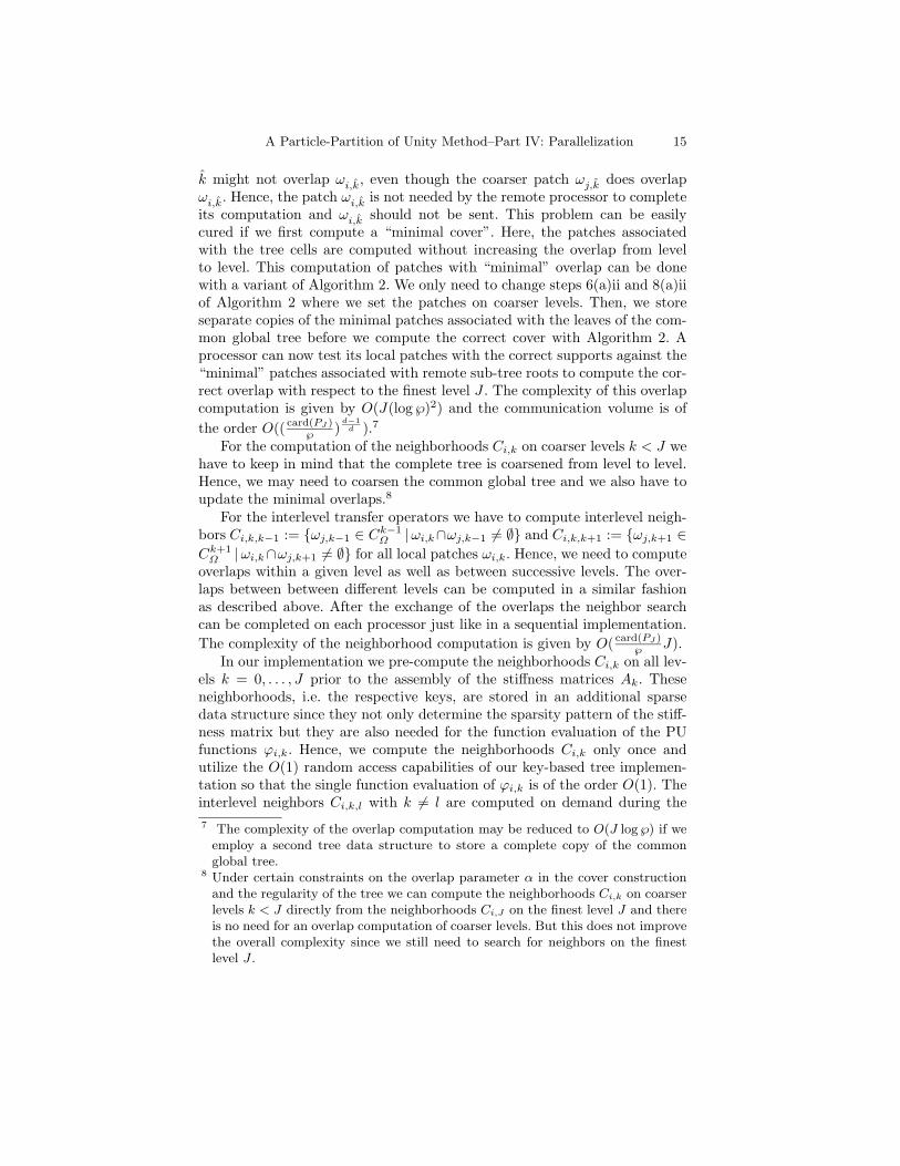
The timing results are given in Table 2 for the stiffness matrix and thetransfer operators, i.e. displayed are the sum of the assembly times on alllevels k = 0, . . . , J . The scaling behavior of these assembly steps are depictedin Figure 5. From the numbers displayed in Table 2, we can observe a perfectspeed-up for the operator setup as well as for both interlevel transfer opera-tors. Note that the setup times for the interlevel transfer operators includesthe assembly times for the prolongation as well as for the restriction.

The scaling behavior of the assembly phase is as expected (almost) per-fect. Here, we see some fluctuations in the execution times due to the effectthe irregularity of the initial point set has on the number of neighbors. Wecan observe that the curves for the operator assembly (Figure 5 (left)) andthe transfer operators based on the Global-to-Local projection (Figure 5 (cen-ter)) are very similar, whereas the curve for the Local-to-Local projectionsis somewhat different (Figure 5 (right)). This is due to the fact that theGlobal-to-Local projection involves all geometric neighboring patches justlike the operator. The Local-to-Local projection, however, involves hierarchi-cal neighbors [9] only. Hence, the fluctuations in the execution times for theLocal-to-Local projections are due to variations in the number of levels of theglobal tree only. But the fluctuations in the measured wall clock times for theassembly of the operators and the Global-to-Local projections stem from thevariation of the local refinement levels which essentially determine the num-ber of neighbors. Furthermore, the assembly of the Global-to-Local transfersinvolves the integration of more complicated integrals than the assembly of


the Local-to-Local transfers, see [9]. Hence, the logarithmic complexity of theneighbor search completed in the assembly of both types of transfer operatorsis not really visible in the curves for the Global-to-Local transfers and justslightly visible in the assembly of the Local-to-Local transfers. Note that theimprovement in the execution times for 128 processors with load = 32768again comes from the use of the Halton point set. Here, the resulting coveris closer to the uniform situation and the overall storage utilization is betterthan for smaller processor numbers.

Multilevel Solution. The parallel scaling behavior of our multilevelsolver should essentially be the same as that of classical multigrid meth-ods for mesh-based discretizations which has been studied in many articles[2, 3, 5, 6, 10, 11, 13, 14, 15, 21, 22]. A classical parallel multigrid solverscales with O( dof

℘ + ( dof℘ )

d−1d + log(dof) + log(℘)). Hence, we expect to see a

logarithmic scaling behavior of our multilevel solver as well.We measure the wall clock times for the solution of the linear system and

divide it by the number of completed iterations r to get the average cycletime. The initial value u0 for the multilevel iteration is random valued with‖u0‖ = 1. The stopping criterion for the iteration is ‖ur‖ < 10−10 or r > 50.The error reduction rate of the iteration is therefore given by ρ := ‖ur‖

1r .

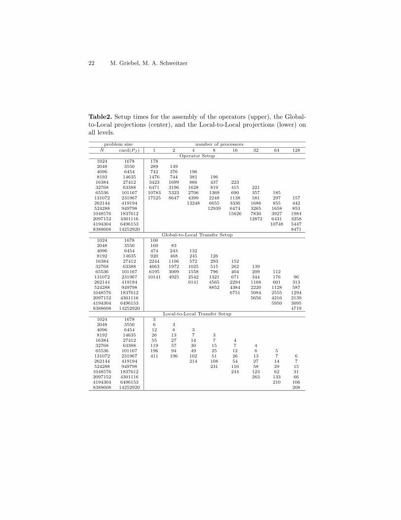
The scaling behavior of the average cycle times are depicted in Figure6 for V (µ, µ)-cycles with µ = 1, 2, 3. These graphs show only a very slightlogarithmic scaling behavior of our multilevel solver. Note that the multileveliteration with the Local-to-Local transfer operators is about 10% faster thanthe corresponding cycle based on the Global-to-Local transfers. This is dueto the different (block-)sparsity patterns of the transfer operators. The ap-plication of the Local-to-Local transfer operators involves less computationalwork and less communication. The difference in the cycles times will probablybe more severe on parallel machines with a less balanced ratio of bandwidthto flops.

The different transfer operators have almost no effect on the error reduc-tion rates ρ, see [9] for further details. But the two different smoothers, thesimple (block-)Jacobi smoother and the composite sub-domain-block-Jacobismoother with internal (block-)Gauß–Seidel iteration, certainly influence theoverall rates ρ. Yet, both smoothers require a similar number of operationsand the same communication so that the cycle times are essentially the samefor both smoothers.

The error reduction rates ρ using the (block-)Jacobi smoother are noteffected by a change of the number of processors since the overall algorithmstays the same independent of the number of processors. But the rates for thecomposite smoother are dependent on the number of processors. For a V (1, 1)-cycle we measure reduction rates ρ between 0.3 and 0.4 for the compositesmoother, and rates of about 0.6 for the (block-)Jacobi smoother. The ratesfor a V (2, 2)-cycle are between 0.1 and 0.2 for the composite smoother, andabout 0.3 for the (block-)Jacobi smoother. With three smoothing steps we


Table2. Setup times for the assembly of the operators (upper), the Global-to-Local projections (center), and the Local-to-Local projections (lower) onall levels.

problem size number of processors

N card(PJ ) 1 2 4 8 16 32 64 128Operator Setup

1024 1678 1782048 3550 289 1494096 6454 742 376 1968192 14635 1476 744 381 19616384 27412 3423 1699 866 437 22332768 63388 6471 3196 1628 819 415 22165536 101167 10783 5323 2706 1369 690 357 185131072 231967 17525 8647 4399 2248 1138 581 297 157262144 419194 13248 6655 3336 1686 855 442524288 949798 12939 6474 3265 1658 8531048576 1837612 15626 7830 3927 19842097152 4301116 12872 6431 32584194304 6496153 10748 54478388608 14252920 8471

Global-to-Local Transfer Setup1024 1678 1002048 3550 160 834096 6454 474 243 1328192 14635 920 468 245 12616384 27412 2244 1106 572 293 15232768 63388 4063 1972 1025 515 262 13965536 101167 6195 3009 1558 796 404 209 112131072 231967 10141 4925 2542 1321 671 344 176 96262144 419194 9141 4565 2294 1168 601 313524288 949798 8852 4384 2220 1128 5871048576 1837612 6751 5084 2555 12942097152 4301116 5656 4216 21394194304 6496153 5950 30958388608 14252920 4719

Local-to-Local Transfer Setup1024 1678 32048 3550 6 34096 6454 12 6 38192 14635 26 13 7 316384 27412 55 27 14 7 432768 63388 119 57 30 15 7 465536 101167 196 94 49 25 12 6 5131072 231967 411 196 102 51 26 13 7 6262144 419194 214 108 54 27 14 7524288 949798 231 116 58 29 151048576 1837612 244 123 62 312097152 4301116 263 133 664194304 6496153 210 1068388608 14252920 208


0 20 40 60 80 100 120

1

2

3

4

5

6

7

8

execution times


seco

nds


0 20 40 60 80 100 120

1

2

3

4

5

6

7

8

9

10

11

execution times


seconds


0 20 40 60 80 100 120

2

4

6

8

10

12

14

execution times


seconds


0 20 40 60 80 100 120

1

2

3

4

5

6

execution times


seco

nds


0 20 40 60 80 100 120

1

2

3

4

5

6

7

8

9

10

execution times


seconds


0 20 40 60 80 100 120

2

4

6

8

10

12

execution times


seconds


Figure6. Execution times for a single V (µ, µ)-cycle with the Global-to-Localprojections (upper) and the Local-to-Local projections (lower). With µ = 1(right), µ = 2 (center), and µ = 3 (right).

measure rates ρ of about 0.1 for the composite smoother, and about 0.2 forthe (block-)Jacobi smoother.

Example 2 (Graded Halton points). In our second experiment we use thesame local approximation spaces V pi,ki,k , the linear Legendre polynomials, butwe use a more irregular initial point set P . Here, we use a grading functionG to transform a Halton point set. The resulting transformed points are thenused as the initial point set P for the cover construction. We use the gradingfunction

G : ξ = (ξi)di=1 ∈ [0, 1]d 7→ a(ξ)ξ ∈ [0, 1]d with a(ξ) =‖ξ‖2 if ‖ξ‖2 ≤ 1

1 else .

Here, our initial uniform decomposition is completely inappropriate and manydata have to be re-balanced. The number of initial points strongly variesamong the processors, e.g. for N = 1048576 and ℘ = 64 we find fromcard(PJ q) = 14206 to card(PJ q) = 214654 points of the finest point setPJ on level J = 21 on different processors q prior to our load balancing.Therefore, we cannot expect the load balancing step itself to scale. The pur-pose of the balancing step is to resolve the load imbalance at low cost sothat the overall algorithm utilizes all available resources for the larger partof the computation. Note that the overall execution time for the complete


0 20 40 60 80 100 120

500

1000

1500

2000

2500

3000

3500

4000

4500

5000

5500

execution times


seconds

load=16384load=8192load=4096load=2048load=1024

0 20 40 60 80 100 120

500

1000

1500

2000

2500

3000

3500

execution times


seconds


0 20 40 60 80 100 120

10

20

30

40

50

60

70

execution times


seconds


Figure7. Setup times for the assembly of the operator (left), the Global-to-Local transfers (center), and the Local-to-Local transfers (right) on alllevels.

balancing step amounts to less than 1% of the time spent in the assembly ofthe discrete operators.

The measured wall clock times for the discretization phase of our PUMfor the graded Halton point set are given in Table 3. From these numberswe can again observe a perfect speed-up for the operator setup as well asfor both interlevel transfer operators. The scaling behavior of these assemblysteps are depicted in Figures 7. Again, we see the anticipated perfect scalingbehavior of the setup phase. Hence, our load balancing step certainly fulfillsits purpose.

Also the scaling behavior of our multilevel solver (see Figure 8) is opti-mal. Here, the convergence rates for a V (1, 1)-cycle with the Local-to-Localtransfers and the composite smoother are between 0.3 and 0.5. The rates ofthe multilevel iteration with the simple (block-)Jacobi smoother are aboutρ = 0.6 for the V (1, 1)-cycle with the Global-to-Local transfers. Note that wemay need more than one smoothing step when we use a simple (block-)Jacobismoother together with the Local-to-Local transfers for highly irregular pointsets, see [9] for details.

5 Concluding Remarks

We presented a parallel meshfree method for the discretization of an ellipticpartial differential equation and the efficient parallel multilevel solution ofthe arising linear (block-)system. The main ingredients of our parallelizationare a key-based tree implementation and the use of a space filling curve loadbalancing scheme.

The discretization phase where the discrete operators are assembled is themost expensive step in our particle-partition of unity method. This specificpart of the method requires no communication at all and its scaling behavioris only dependent on the quality of the data partition. Hence, our load bal-ancing scheme is aimed to balance this most expensive part of the method.


Table3. Setup times for the assembly of the operators (upper), the Global-to-Local projections (center), and the Local-to-Local projections (lower) onall levels.

problem size number of processors

N card(PJ ) 1 2 4 8 16 32 64 128Operator Setup

1024 1942 2542048 3643 430 2364096 7522 947 500 2718192 14986 1901 997 522 28216384 31495 4304 2194 1144 619 32732768 62542 4466 2292 1239 640 33465536 121966 4495 2437 1263 678 358131072 242506 4661 2411 1242 659 339262144 484435 5103 2673 1361 710524288 972988 5155 2652 13761048576 1976116 5460 28052097152 3976408 5272

Global-to-Local Transfer Setup1024 1942 1682048 3643 270 1544096 7522 590 321 1868192 14986 1171 624 343 19216384 31495 2748 1424 766 419 22732768 62542 2859 1507 848 427 23465536 121966 3062 1663 868 473 259131072 242506 3123 1651 879 484 250262144 484435 3422 1832 949 514524288 972988 3650 1906 10151048576 1976116 3675 19332097152 3976408 3540

Local-to-Local Transfer Setup1024 1942 42048 3643 7 44096 7522 15 7 48192 14986 30 15 8 416384 31495 65 31 17 8 432768 62542 63 33 17 9 465536 121966 64 33 17 9 5131072 242506 65 33 17 9 5262144 484435 68 35 18 9524288 972988 69 35 181048576 1976116 72 372097152 3976408 72


0 20 40 60 80 100 120

0.5

1

1.5

2

2.5

3

3.5

4

4.5

execution times


seconds


0 20 40 60 80 100 120

1

2

3

4

5

6

execution times


seco

nds


0 20 40 60 80 100 120

1

2

3

4

5

6

7

8

execution times


seco

nds


0 20 40 60 80 100 120

0.5

1

1.5

2

2.5

3

3.5

execution times


seconds


0 20 40 60 80 100 120

0.5

1

1.5

2

2.5

3

3.5

4

4.5

5

5.5

execution times


seconds


0 20 40 60 80 100 120

1

2

3

4

5

6

7

execution times


seco

nds


Figure8. Execution times for a single V (µ, µ)-cycle with the Global-to-Localprojections (upper) and the Local-to-Local projections (lower). With µ = 1(right), µ = 2 (center), and µ = 3 (right).

The results of our numerical experiments showed that (within the expectedfluctuations) we achieve a perfect scaling behavior. All other parts of themethod, the computation of the load estimate, the setup of the transfer op-erators (at least the setup of the Local-to-Local transfers) and the multilevelsolution are completely negligible with respect to execution times. Yet, ourdata partition also allows for the optimal scaling behavior of each of thesesteps. The presented space filling curve balancing scheme provides high qual-ity data partitions independent of the number and distribution of points ata very low computational cost.

References

[1] I. Babuska, U. Banerjee, and J. E. Osborn, Meshless and Gen-eralized Finite Element Methods: A Survey of Some Major Results, inMeshfree Methods for Partial Differential Equations, Lecture Notes inComputational Science and Engineering, Springer, 2002.

[2] P. Bastian, Load Balancing for Adaptive Multigrid Methods, SIAM J.Sci. Comp., 19 (1998), pp. 1303–1321.

[3] A. Brandt, Multigrid Solvers on Parallel Computers, in Elliptic Prob-lem Solvers, M. H. Schultz, ed., Academic Press, 1981, pp. 39–83.


[4] A. Caglar, M. Griebel, M. A. Schweitzer, and G. W. Zum-

busch, Dynamic Load-Balancing of Hierarchical Tree Algorithms on aCluster of Multiprocessor PCs and on the Cray T3E, in Proceedings 14thSupercomputer Conference, Mannheim, H. W. Meuer, ed., Mannheim,Germany, 1999, Mateo.

[5] M. Griebel, Parallel Domain-Oriented Multilevel Methods, SIAM J.Sci. Comp., 16 (1995), pp. 1105–1125.

[6] M. Griebel and T. Neunhoeffer, Parallel Point- and Domain-Oriented Multilevel Methods for Elliptic PDE on Workstation Networks,J. Comp. Appl. Math., 66 (1996), pp. 267–278.

[7] M. Griebel and M. A. Schweitzer, A Particle-Partition of UnityMethod for the Solution of Elliptic, Parabolic and Hyperbolic PDE, SIAMJ. Sci. Comp., 22 (2000), pp. 853–890.

[8] , A Particle-Partition of Unity Method—Part II: Efficient CoverConstruction and Reliable Integration, SIAM J. Sci. Comp., 23 (2002),pp. 1655–1682.

[9] , A Particle-Partition of Unity Method—Part III: A MultilevelSolver, SIAM J. Sci. Comp., (2002). to appear.

[10] M. Griebel and G. W. Zumbusch, Hash-Storage Techniques forAdaptive Multilevel Solvers and their Domain Decomposition Paralleliza-tion, in Domain Decomposition Methods 10, The 10th International Con-ference, Boulder, J. Mandel, C. Farhat, and X.-C. Cai, eds., vol. 218 ofContemp. Math., AMS, 1998, pp. 271–278.

[11] C. E. Grosch, Poisson Solvers on Large Array Computers, in Proc.1978 LANL Workshop on Vector and Parallel Processors, B. L. Buzbeeand J. F. Morrison, eds., 1978.

[12] F. C. Gunther and W. K. Liu, Implementation of Boundary Con-ditions for Meshless Methods, Comput. Meth. Appl. Mech. Engrg., 163(1998), pp. 205–230.

[13] J. E. Jones and S. F. McCormick, Parallel Multigrid Meth-ods, in Parallel Numerical Algorithms, D. E. Keyes, A. Sameh, andV. Venkatakrishnan, eds., Kluwer Academic Publishers, 1997, pp. 203–224.

[14] O. A. McBryan, P. O. Frederickson, J. Linden, A. Schuller,

K. Solchenbach, K. Stuben, C. A. Thole, and U. Trotten-

berg, Multigrid Methods on Parallel Computers – A Survey of RecentDevelopments, IMPACT Comput. Sci. Engrg., 3 (1991), pp. 1–75.

[15] W. F. Mitchell, A Parallel Multigrid Method using the Full DomainPartition, Electron. Trans. Numer. Anal., 6 (1997), pp. 224–233. SpecialIssue for Proc. of the 8th Copper Mountain Conf. on Multigrid Methods.

[16] J. Nitsche, Uber ein Variationsprinzip zur Losung von Dirichlet-Problemen bei Verwendung von Teilraumen, die keinen Randbedingun-gen unterworfen sind, Abh. Math. Univ. Hamburg, 36 (1970–1971),pp. 9–15.

[17] A. Pothen, Graph Partitioning Algorithms with Applications to Sci-entific Computing, in Parallel Numerical Algorithms, D. E. Keyes,


A. Sameh, and V. Venkatakrishnan, eds., Kluwer Academic Publishers,1997, pp. 323–368.

[18] H. Sagan, Space-Filling Curves, Springer, New York, 1994.[19] M. A. Schweitzer, Ein Partikel–Galerkin–Verfahren mit Ansatzfunk-

tionen der Partition of Unity Method, Diplomarbeit, Institut fur Ange-wandte Mathematik, Universitat Bonn, 1997.

[20] M. A. Schweitzer, G. W. Zumbusch, and M. Griebel, Parnass2:A Cluster of Dual-Processor PCs, in Proceedings of the 2nd WorkshopCluster-Computing, Karlsruhe, W. Rehm and T. Ungerer, eds., no. CSR-99-02 in Chemnitzer Informatik Berichte, Chemnitz, Germany, 1999, TUChemnitz, pp. 45–54.

[21] K. Solchenbach, C. A. Thole, and U. Trottenberg, ParallelMultigrid Methods: Implementation on SUPRENUM–like architecturesand applications, in Supercomputing, vol. 297 of Lecture Notes in Com-puter Science, Springer, 1987, pp. 28–42.

[22] L. Stals, Parallel Implementation of Multigrid Methods, PhD thesis,Department of Mathematics, Australian National University, 1995.

[23] M. S. Warren and J. K. Salmon, A Parallel Hashed Oct-TreeN-Body Algorithm, in Supercomputing ’93, Los Alamitos, 1993, IEEEComp. Soc., pp. 12–21.

[24] , A Portable Parallel Particle Program, Computer Physics Com-munications, 87 (1995).

[25] , Parallel, Out-of-core Methods for N-body Simulation, in Proceed-ings of the 8th SIAM Conference on Parallel Processing for ScientificComputing, M. Heath, V. Torczon, G. Astfalk, P. . E. Bjørstad, A. H.Karp, C. H. Koebel, V. Kumar, R. F. Lucas, L. T. Watson, and D. E.Womble, eds., Philadelphia, 1997, SIAM.

[26] G. W. Zumbusch, Simultanous h-p Adaptation in Multilevel Finite Ele-ments, dissertation, Fachbereich Mathematik und Informatik, FU Berlin,1995.

[27] , Adaptive Parallel Multilevel Methods for Partial DifferentialEquations, Habilitation, Insitut fur Angewandte Mathematik, Univer-sitat Bonn, 2001.

[28] , On the Quality of Space-Filling Curve Induced Partitions, Z.Angew. Math. Mech., 81 Suppl. 1 (2001), pp. 25–28.

Documents

A Particle-Partition of Unity Method{Part IV: Parallelizationwissrech.ins.uni-bonn.de/research/pub/schweitzer/... · · 2015-03-23A Particle-Partition of Unity Method{Part IV: Parallelization