Embed Size (px)
Citation preview

Research ArticleAn Analytical Solution for Predicting the Vibration-Fatigue-Lifein Bimodal Random Processes
Chaoshuai Han1 Yongliang Ma1 Xianqiang Qu1 and Mindong Yang2
1College of Shipbuilding Engineering Harbin Engineering University Harbin Heilongjiang 150001 China2Guangdong Electric Power Design Institute Co Ltd of China Energy Engineering Group Guangzhou China
Correspondence should be addressed to Yongliang Ma mayonglianghrbeueducn
Received 6 September 2016 Accepted 26 December 2016 Published 31 January 2017
Academic Editor Nuno M Maia
Copyright copy 2017 Chaoshuai Han et alThis is an open access article distributed under the Creative Commons Attribution Licensewhich permits unrestricted use distribution and reproduction in any medium provided the original work is properly cited
Predicting the vibration-fatigue-life of engineering structures subjected to random loading is a critical issue for Frequencymethodsare generally adopted to deal with this problemThis paper focuses on bimodal spectra methods including Jiao-Moanmethod Fu-Cebon method and Modified Fu-Cebon method It has been proven that these three methods can give acceptable fatigue damageresults However these three bimodal methods do not have analytical solutions Jiao-Moan method uses an approximate solutionFu-Cebon method and Modified Fu-Cebon method needed to be calculated by numerical integration which is obviously notconvenient in engineering application Thus an analytical solution for predicting the vibration-fatigue-life in bimodal spectra isdeveloped The accuracy of the analytical solution is compared with numerical integration The results show that a very goodagreement between an analytical solution and numerical integration can be obtained Finally case study in offshore structures isconducted and a bandwidth correction factor is computed through using the proposed analytical solution
1 Introduction
Engineering structures from different fields (eg aircraftswind energy utilizations and automobiles) are commonlysubjected to random vibration loading These loads oftencause structural fatigue failure Thus it is significant to carryout a study on assessing the vibration-fatigue-life [1 2]
Vibration fatigue analysis commonly consists of two partprocesses structural dynamic analysis and results postpro-cessing Structural dynamic analysis provides an accurateprediction of the stress responses of fatigue hot-spots Oncethe stress responses are obtained vibration fatigue can besuccessfully performed Existing technologies such as oper-ational modal analysis [3] finite element modeling (FEM)and accelerated-vibration-tests are mature and applicableto obtain the stress of structures [4 5] Therefore thecrucial part of a vibration fatigue analysis focuses on resultspostprocessing
The postprocessing is usually used to calculate fatiguedamage based on known stress responses When the stressresponses are time series fatigue can be evaluated using a tra-ditional time domain method However the stress responses
of real structures are mostly characterized by the powerspectral density (PSD) function Thus frequency domainmethod becomes popular in vibration fatigue analysis [6 7]
A bimodal spectrum is a particular PSD in the randomvibration stress response of a structure For some simplestructures the stress response of structures will show explicitcharacterization of two peaks One peak of the bimodalspectrum is governed by the first-order natural frequency ofthe structure another is dominated by the main frequency ofapplied loads Therefore some bimodal methods for fatigueanalysis can be adopted [8ndash10] Moreover several experi-ments (eg vibration tests on mechanical components) andnumerical studies (eg virtual simulation of dynamic usingFEM) also obtain have shown that the stress PSD is a typicalbimodal spectrum [5 7 11] However for some complexflexible structures the PSDof the stress response of structuresusually is a multimodal and wide-band spectrum For thissituation existing general wide-band spectral methods suchas Dirlik method [12] Benasciutti-Tovo method [10] andPark method [13 14] can be used to evaluate the vibration-fatigue-life Recently Braccesi et al [15 16] proposed a bands
HindawiShock and VibrationVolume 2017 Article ID 1010726 18 pageshttpsdoiorg10115520171010726
2 Shock and Vibration
method to estimate the fatigue damage of a wide-bandrandom process in the frequency domain In order to speedup the frequency domain method Braccesi et al [17 18]developed a modal approach for fatigue damage evaluationof flexible components by FEM
For fatigue evaluation in bimodal processes some specificformulae have been proposed Jiao and Moan [8] provideda bandwidth correction factor from a probabilistic point ofview and the factor is an approximate solution derived bythe original model The approximation inevitably leads tosome errors in certain cases Based on an similar idea Fuand Cebon [9] developed a formula for predicting the fatiguelife in bimodal random processes In the formula there isa convolution integral The author claimed that there is noanalytical solution for the convolution integral which hasto be calculated by numerical integration Benasciutti andTovo [10] compared the above twomethods and established aModified Fu-Cebon method The new formula improves thedamage estimation but it still needs to calculate numericalintegration
In engineering application the designers prefer an analyt-ical solution rather than numerical methods Therefore thepurpose of this paper is to develop an analytical solution topredict the vibration-fatigue-life in bimodal spectra
2 Theory of Fatigue Analysis
21 Fatigue Analysis The basic 119878-119873 curve for fatigue analysiscan be given as
119873 = 119870 sdot 119878minus119898 (1)
where 119878 represents the stress amplitude 119873 is the number ofcycles to fatigue failure and119870 and119898 are the fatigue strengthcoefficient and fatigue strength exponent respectively
The total fatigue damage can then be calculated as a linearaccumulation rule after Miner [19]
119863 = sum 119899119894119873119894= 1119870sum119899119894119878119898119894 (2)
where 119899119894 is the number of cycles in the stress amplitude 119878119894resulting from rainflow counting (RFC) [20] and 119873119894 is thenumber of cycles corresponding to fatigue failure at the samestress amplitude
When the stress amplitude is a continuum function andits probability density function (PDF) is 119891119878(119878) the fatiguedamage in the duration 119879 can be denoted as follows
119863 = ]119888 sdot 119879119870 intinfin
0119878119898 sdot 119891119878 (119878) 119889119878 (3)
where ]119888 is the frequency of rainflow cyclesFor an ideal narrowband process 119891119878(119878) can be approxi-
mated by the Rayleigh distribution [21] the analytical expres-sion is given as
119891119878 (119878) = 1198781205820 exp(minus 119878221205820) (4)
Furthermore the frequency of rainflow cycles ]119888 can bereplaced by rate of mean zero upcrossing ]0
According to (3) an analytical solution of fatigue damage[22] for an ideal narrowband process can be written as
119863NB = ]0 sdot 119879119870 (radic21205820)119898 Γ (1198982 + 1) (5)
where Γ(sdot) is the Gamma functionFor general wide-band stress process fatigue damage can
be calculated by a narrowband approximation (ie (5)) firstand bandwidth correction is made based on the followingmodel [23]
119863WB = 120588 sdot 119863NB (6)
In general bimodal process is a wide-band process thusthe fatigue damage in bimodal process can be calculatedthrough (6)
22 Basic Principle of Bimodal SpectrumProcess Assume thata bimodal stress process119883(119905) is composed of a low frequencyprocess (LF)119883119871(119905) and a high frequency process (HF)119883119867(119905)119883(119905) = 119883119871 (119905) + 119883119867 (119905) (7)
where 119883119871(119905) and 119883119867(119905) are independent and narrow Gaus-sian process
The one-sided spectral density function of 119883(119905) can besummed from the PSD of LF and HF process
119878 (120596) = 119878119871 (120596) + 119878119867 (120596) (8)
The 119894th-order spectral moments of 119878(120596) are defined as
120582119894 = intinfin
0120596119894 sdot [119878119871 (120596) + 119878119867 (120596)] 119889120596 = 120582119894119871 + 120582119894119867 (9)
The rate of mean zero upcrossing corresponding to119883119871(119905)and119883119867(119905) is
]0119871 = 12120587radic12058221198711205820119871 ]0119867 = 12120587radic12058221198671205820119867
(10)
The rate ofmean zero upcrossing of119883(119905) can be expressedas
]0 = 12120587radic1205822119871 + 12058221198671205820119871 + 1205820119867 = radic ]201198711205820119871 + ]2011986712058201198671205820119871 + 1205820119867 (11)
According to (5) (9) and (11) narrowband approxima-tion of bimodal stress process119883(119905) can be given as
119863NB119883 = radic ]201198711205820119871 + ]2011986712058201198671205820119871 + 1205820119867 119879119870 (radic21205820119871 + 21205820119867)119898
sdot Γ (1198982 + 1) (12)
Shock and Vibration 3
Equation (12) is known as the combined spectrummethod inAPI specifications [24]
The existing bimodal methods proposed by Jiao andMoan Fu and Cebon and Benasciutti and Tovo are basedon the idea two types of cycles can be extracted from therainflow counting one is the large stress cycle and the other isthe small cycle [8ndash10]The fatigue damage due to119883(119905) can beapproximated with the sum of two individual contributions
119863 = 119863119897 + 119863119904 (13)
where 119863119897 represents the damage due to the large stress cycleand119863119904 denotes the damage due to the small stress cycle
3 A Review of Bimodal Methods
31 Jiao-Moan (JM) Method To simplify the study 119883(119905)119883119871(119905) and 119883119867(119905) are normalized as 119883lowast(119905) 119883lowast119871(119905) and 119883lowast
119867(119905)through the following transformation
119883lowast (119905) = 119883 (119905)radic1205820 = 119883119871 (119905)radic1205820 + 119883119867 (119905)radic1205820 = 119883lowast119871 (119905) + 119883lowast
119867 (119905) (14)
and then
120582lowast0 = 120582lowast0119871 + 120582lowast0119867 = 1 (15)
where
120582lowast0119871 = 12058201198711205820 120582lowast0119867 = 12058201198671205820 (16)
Jiao-Moan points out that the small stress cycles areproduced by the envelope of the HF process which followstheRayleigh distributionThe fatigue damage due to the smallstress cycles can be obtained according to (5)
While the large stress cycles are from the envelop process119875(119905) (see Figure 1) the amplitude of 119875(119905) is equal to119876 (119905) = 119877119871 (119905) + 119877119867 (119905) (17)
where 119877119871(119905) and 119877119867(119905) are the envelopes of119883lowast119871(119905) and119883lowast
119867(119905)respectively
The distribution of 119876(119905) can be written as a form of aconvolution integral
119891119876 (119902) = int119902
0119891119877119871 (119902 minus 119909) 119891119877119867 (119909) 119889119909
= int119902
0119891119877119871 (119910) 119891119877119867 (119902 minus 119910) 119889119910 (18)
minus3
minus2
minus1
0
1
2
3
4
Stre
ss
1 2 3 4 5 6 7 8 9 100t
XlowastL(t) + Xlowast
H(t)Envelope P(t)Amplitude Q(t)
Figure 1 Bimodal process119883lowast(119905) the envelope process 119875(119905) and theamplitude process 119876(119905)
119877119871(119905) and119877119867(119905) obey theRayleigh distribution therefore (18)has an analytical solution which is given [8]
119891119876 (119902) = 119902120582lowast0119871 sdot exp(minus 11990222120582lowast0119871) + 119902120582lowast0119867sdot exp(minus 11990222120582lowast0119867) + exp(minus11990222 )sdot radic2120587120582lowast0119871120582lowast0119867sdot [[Φ(119902radic 120582lowast0119871120582lowast0119867) + Φ(119902radic120582lowast0119867120582lowast0119871 ) minus 1]]sdot (1199022 minus 1)
(19)
The rate of mean zero upcrossing due to 119875(119905) can becalculated as
]0119875 = 120582lowast0119871]0119871radic1 + 120582lowast0119867120582lowast0119871 (]0119867]0119871
120575119867)2 (20)
where
120575119867 = radic1 minus 120582lowast11198672
120582lowast0119867120582lowast2119867 (21)
An approximation was made by Jiao andMoan for (19) asfollows [8]
119891119876 (119902) asymp (120582lowast0119871 minus radic120582lowast0119871120582lowast0119867) sdot 119902 sdot exp(minus 11990222120582lowast0119871)+ radic2120587120582lowast0119871120582lowast0119867 sdot (1199022 minus 1) sdot exp(minus11990222 )
(22)
4 Shock and Vibration
Table 1 Comparison of large cycles and small cycles for different spectral methods
Method Large cycles Small cycles119899119897 PDF of amplitude 119899119904 PDF of amplitudeJM ]0119875 sdot 119879 Eq (22) ]0119867 sdot 119879 RayleighFC ]0119871 sdot 119879 Eq (25) (]0119867 minus ]0119871) sdot 119879 RayleighMFC ]0119875 sdot 119879 Eq (25) (]0119867 minus ]0119875) sdot 119879 Rayleigh
minus3
minus2
minus1
0
1
2
3
Stre
ss
12 14 15 16 17 18 19 20 21 22 2313t
SL + SH
SH
XL + XH
Figure 2 The large cycles and small cycles for a random stressprocess
After the approximation a closed-form solution of thebandwidth correction factor can be then derived [8]
120588 = ]0119875]0
times [[120582lowast0119871
1198982+2(1 minus radic120582lowast0119867120582lowast0119871 )
+ radic120587120582lowast0119871120582lowast0119867119898Γ (1198982 + 12)Γ (1198982 + 1) ]] + ]0119867]0
120582lowast01198671198982(23)
Finally the fatigue damage can be obtained as (6) and (12)
32 Fu-Cebon (FC) Method Similarly to JM method Fu andCebon also considered that the total damage is produced bya large cycle (119878119867 + 119878119871) and a small cycle (119878119871) as depicted inFigure 2 The small cycles are from the HF process and thedistribution of the amplitude119875119878119904(119878) is a Rayleigh distributionas shown in (4) However the number of cycles associatedwith the small cycles 119899119904 is different from JM method andequals (]0119867 minus ]0119871) sdot 119879 According to (5) the damage due tothe small cycles is
119863119904 = (]0119867 minus ]0119871) sdot 119879119870 (radic21205820119867)119898 Γ (1 + 1198982 ) (24)
The amplitude of the large cycles 119878119897 can be approximatedas the sum of amplitude of the LF and HF processes the
distribution of which can be expressed by a convolution oftwo Rayleigh distributions [9]
119875119878119897 (119878) = int119878
0119875119878119871 (119910) 119875119878119867 (119878 minus 119910) 119889119910
= int119878
0119875119878119871 (119878 minus 119910) 119875119878119867 (119910) 119889119910
= 112058201198711205820119867 119890minus1198782(21205820119867) int119878
0(119878119910 minus 1199102) 119890minus1198801199102+119881119878119910119889119910
(25)
where 119880 = 121205820119871 + 121205820119867 and 119881 = 11205820119867The number of cycles of the large cycles is 119899119897 = ]0119871 sdot 119879
Thus the fatigue damage due to the large stress cycles can beexpressed by
119863119897 = ]0119871 sdot 119879119870 intinfin
0119878119898119875119878119897 (119878) 119889119878 (26)
Equation (26) can be calculated with numerical integra-tion [9 10] Therefore the total damage can be obtainedaccording to (13)
33 Modify Fu-Cebon (MFC) Method Benasciutti and Tovomade a comparison between JMmethod and FCmethod andconcluded that using the envelop process is more suitable[10] Thus a hybrid technique is adopted to modify theFC method More specifically the large cycles and smallcycles are produced according to the idea of FC method Thenumber of cycles associated with the large cycles is definedsimilarly to JM method That is 119899119897 = ]0119875 sdot 119879 while thenumber of cycles corresponding to the small cycles is 119899119904 =(]0119867 minus ]0119875) sdot 119879 The total damage for MFC method can bethen written according to (13)
Although the accuracy of the MFC method is improvedthe fatigue damage still has to be calculated with numericalintegral
34 Comparison of Three Bimodal Methods Detailed com-parison of the aforementioned three bimodal methods can befound in Table 1 In all methods the amplitude of the smallcycle obeys Rayleigh distribution and the correspondingfatigue damage has an analytical expression as in (5) thedistribution of amplitude of the large cycle is convolutionintegration of two Rayleigh distributions and the relevantfatigue damage can be calculated by (26)
Because of complexity of the convolution integrationseveral researches assert that (26) has no analytical solution[9 10] To solve this problem Jiao andMoan used an approx-imate model (ie (22)) to obtain a closed-form solution [8]
Shock and Vibration 5
Eq (22)Eq (19)
1 2 3 4 50q
fQ
(q)
120582lowast0L = 001 120582lowast
0H = 099
minus03
minus02
minus01
0
01
02
03
04
05
06
07
(a)
Eq (22)Eq (19)
1 2 3 4 50q
fQ
(q)
120582lowast0L = 099 120582lowast
0H = 001
minus03
minus02
minus01
0
01
02
03
04
05
06
07
(b)
Figure 3 The divergence of (19) and (22) for JM method in case of (a) 120582lowast0119871 = 001 and (b) 120582lowast0119871 = 099However the approximate model may lead to errors in somecases as in Figure 3 which illustrates the divergence of (19)and (22) for different values of 120582lowast0119871 and 120582lowast0119867 It is found that(22) becomes closer to (19) with the increase of 120582lowast0119871
For FC andMFCmethods (26) was calculated by numer-ical technique Although the numerical technique can give afatigue damage prediction it is complex and not convenientwhen applied in real engineering In addition the solutionsin some cases are not reasonable In Section 4 an analyticalsolution of (26)will be derived to evaluate the fatigue damageand the derivation of the analytical solution focuses on thefatigue damage of the large cycles
4 Derivation of an Analytical Solution
41 Derivation of an Analytical Solution for (25) Equation(25) can be rewritten as
119875119878119897 (119878) = int119878
0
11991011987812058201198711205820119867 exp(minus 119910221205820119867)sdot exp[minus(119878 minus 119910)221205820119871 ]119889119910minus int119878
0
119910212058201198711205820119867 exp(minus 119910221205820119867)sdot exp[minus(119878 minus 119910)221205820119871 ]119889119910
(27)
Equation (27) will be divided into two items
(1) The First Item It is as follows
1198681 = int119878
0
11991011987812058201198711205820119867 exp(minus 119910221205820119867)sdot exp[minus(119878 minus 119910)221205820119871 ]119889119910 = minus 1198781205820119871 + 1205820119867sdot exp(minus 119878221205820119867) + 1198781205820119871 + 1205820119867 sdot exp(minus 119878221205820119871)+ 11987821205820119871 (1205820119871 + 1205820119867) sdot radic
2120587120582011987112058201198671205820119871 + 1205820119867sdot exp[minus 11987822 (1205820119871 + 1205820119867)]sdot [Φ(119878radic 12058201198711205820119867 (1205820119871 + 1205820119867)) minus 1+ Φ(119878radic 12058201198671205820119871 (1205820119871 + 1205820119867))]
(28)
(2) The Second Item It is as follows
1198682 = int119878
0
119910212058201198711205820119867 exp(minus 119910221205820119867)sdot exp[minus(119878 minus 119910)221205820119871 ]119889119910 = minus 1198781205820119871(1205820119871 + 1205820119867)2
6 Shock and Vibration
sdot exp(minus 119878221205820119867) minus 1198781205820119867(1205820119871 + 1205820119867)2 exp(minus119878221205820119871)
minus 21198781205820119867(1205820119871 + 1205820119867)2 [exp(minus119878221205820119867)
minus exp(minus 119878221205820119871)] + exp[minus 11987822 (1205820119871 + 1205820119867)]sdot radic 2120587120582011987112058201198671205820119871 + 1205820119867 [[Φ(119878radic 12058201198711205820119867 (12058201198711 + 1205820119867))
minus 1 + Φ(119878radic 12058201198671205820119871 (1205820119871 + 1205820119867))]][ 11205820119871 + 1205820119867+ 119878212058201198671205820119871 (1205820119871 + 1205820119867)2]
(29)The analytical solution of (25) can be then obtained
119875119878119897 (119878) = 1198781205820119871(1205820119871 + 1205820119867)2 exp(minus119878221205820119871)
+ 1198781205820119867(1205820119871 + 1205820119867)2 exp(minus119878221205820119867)
+ 1198782 minus (1205820119871 + 1205820119867)(1205820119871 + 1205820119867)2 radic2120587120582011987112058201198671205820119871 + 1205820119867sdot exp[minus 11987822 (1205820119871 + 1205820119867)]sdot [Φ(119878radic 12058201198711205820119867 (1205820119871 + 1205820119867)) minus 1+ Φ(119878radic 12058201198671205820119871 (1205820119871 + 1205820119867))]
(30)
Note that when 1205820119871 + 1205820119867 = 1 (30) is just equal to (19)derived by Jiao and Moan [8] Therefore (19) is a special caseof (30)
42 Derivation of anAnalytical Solution for (26) Based on (30)Thederivation of an analytical solution for (26) is on the basisof (30) as
119885 = intinfin
0119878119898 sdot 119875119878119897 (119878) 119889119878 = intinfin
0119878119898 sdot [ 1198781205820119871(1205820119871 + 1205820119867)2
sdot exp(minus 119878221205820119871) + 1198781205820119867(1205820119871 + 1205820119867)2sdot exp(minus 119878221205820119867)]119889119878 + intinfin
0119878119898
sdot 1198782 minus (1205820119871 + 1205820119867)(1205820119871 + 1205820119867)2 radic2120587120582011987112058201198671205820119871 + 1205820119867sdot exp[minus 11987822 (1205820119871 + 1205820119867)]sdot [Φ(119878radic 12058201198711205820119867 (1205820119871 + 1205820119867)) minus 1+ Φ(119878radic 12058201198671205820119871 (1205820119871 + 1205820119867))]119889119878
(31)
Equation (31) will be divided into five parts
(1) The First Part It is as follows
1198851 = intinfin
0119878119898 sdot [ 1198781205820119871(1205820119871 + 1205820119867)2 exp(minus
119878221205820119871)]119889119878= 12058220119871(1205820119871 + 1205820119867)2 sdot (radic21205820119871)119898 sdot Γ (1 + 1198982 )
(32)
(2) The Second Part It is as follows
1198852 = intinfin
0119878119898 sdot [ 1198781205820119867(1205820119871 + 1205820119867)2 exp(minus
119878221205820119867)]119889119878= 12058220119867(1205820119871 + 1205820119867)2 sdot (radic21205820119867)119898 sdot Γ (1 + 1198982 )
(33)
(3) TheThird Part It is as follows
1198853 = 1(1205820119871 + 1205820119867)2sdot radic 2120587120582011987112058201198671205820119871 + 1205820119867 intinfin
0[119878119898+2 minus 119878119898 (1205820119871 + 1205820119867)]
sdot exp[minus 11987822 (1205820119871 + 1205820119867)] 119889119878= 119898radic212058712058211205822 (radic1205820119871 + 1205820119867)119898minus2 (radic2)119898minus1sdot Γ (119898 + 12 )
(34)
(4) The Fourth Part It is as follows
1198854 = intinfin
0119878119898 sdot 1198782 minus (1205820119871 + 1205820119867)(1205820119871 + 1205820119867)2 radic2120587120582011987112058201198671205820119871 + 1205820119867
sdot exp[minus 11987822 (1205820119871 + 1205820119867)]sdot Φ(119878radic 12058201198711205820119867 (1205820119871 + 1205820119867))119889119878
(35)
Shock and Vibration 7
Equation (35) contains a standard Normal cumulativedistribution function Φ(sdot) It is difficult to get an exactsolution directly Thus a new variable is introduced asfollows
119905 = 119878radic1205820119871 + 1205820119867 (36)
With amethod of variable substitution (35) can be simplified
1198854 = radic212058712058201198711205820119867 (radic1205820119871 + 1205820119867)119898minus2sdot [intinfin
0119905119898+2 exp(minus11990522 )Φ(119905radic 12058201198711205820119867)119889119905
minus intinfin
0119905119898 exp(minus11990522 )Φ(119905radic 12058201198711205820119867)119889119905]
(37)
By defining
119867(1205820119871 1205820119867 119898)= intinfin
0119905119898 exp(minus11990522 )Φ(119905radic 12058201198711205820119867)119889119905 (38)
(37) becomes
1198854 = radic212058712058201198711205820119867 (radic1205820119871 + 1205820119867)119898minus2sdot [119867 (1205820119871 1205820119867 119898 + 2) minus 119867 (1205820119871 1205820119867 119898)] (39)
and using integration by parts (38) reduces to
119867(1205820119871 1205820119867 119898)= (119898 minus 1) sdot 119867 (1205820119871 1205820119867 119898 minus 2)
+ 12 1radic2120587radic 12058201198711205820119867 (radic 212058201198671205820119871 + 1205820119867)119898 Γ (1198982 ) (40)
Equation (40) is a recurrence formula when119898 is an oddnumber it becomes
119867(1205820119871 1205820119867 119898) = (119898 minus 1) sdot 119867 (1205820119871 1205820119867 1)+ radic 12058201198711205820119867 (119898 minus 1)2radic2120587sdot (119898+1)2sum
119896=2
1(2119896 minus 2) (radic 212058201198671205820119871 + 1205820119867)2119896minus1 Γ(2119896 minus 12 ) (41)
where (sdot) is a double factorial function and 119867(1205820119871 1205820119867 1)has an analytical expression which can be derived conve-niently
119867(1205820119871 1205820119867 1) = 12 + 12 (radic 12058201198711205820119871 + 1205820119867) (42)
When119898 is an even number119867(1205820119871 1205820119867 119898) is119867(1205820119871 1205820119867 119898) = (119898 minus 1) sdot 119867 (1205820119871 1205820119867 0)
+ radic 12058201198711205820119867 (119898 minus 1)2radic2120587sdot 1198982sum119896=1
1(2119896 minus 1) (radic 212058201198671205820119871 + 1205820119867)2119896 Γ (119896) (43)
where
119867(1205820119871 1205820119867 0) = radic21205874+ 1radic2120587 [1205872 minus atan(radic12058201198671205820119871 )] (44)
Specific derivation of (44) can be seen in Appendix AIn addition a Matlab program has been written to
calculate119867(1205820119871 1205820119867 119898) in Appendix B
(5) The Fifth Part It is as follows
1198855 = intinfin
0119878119898 sdot 1198782 minus (1205820119871 + 1205820119867)(1205820119871 + 1205820119867)2 radic2120587120582011987112058201198671205820119871 + 1205820119867
sdot exp[minus 11987822 (1205820119871 + 1205820119867)]sdot Φ(119878radic 12058201198671205820119871 (1205820119871 + 1205820119867))119889119878
(45)
Similarly to the fourth part the analytical solution of thefifth part can be derived as
1198855 = radic212058712058201198711205820119867 (radic1205820119871 + 1205820119867)119898minus2sdot [119867 (1205820119867 1205820119871 119898 + 2) minus 119867 (1205820119867 1205820119871 119898)] (46)
The final solution is
119885 = 1198851 + 1198852 minus 1198853 + 1198854 + 1198855 (47)
5 Numerical Validation
In this part the accuracy of FC method and JM methodand the derived analytical solution will be validated withnumerical integration Transformation of (26) will be carriedout first
51 Treatment of Double Integral Based on FC Method Aspointed out by Fu and Cebon and Benasciutti and Tovo[9 10] FCrsquos numerical integration can be calculated as thefollowing processes
Equation (26) contains a double integral in which vari-ables 119878 and119910 are in the range of (0infin) and (0 119878) respectivelyApparently the latter is not compatible with the integration
8 Shock and Vibration
range of Gauss-Legendre quadrature formula Therefore byusing a integration transformation
119910 = 1198782 (1 + 119905) (48)
the integral part of (26) can be simplified to
119869 = intinfin
0119878119898119875119878119897 (119878) 119889119878 = 112058201198711205820119867 intinfin
0int1
minus1119878119898 (1198782)
3
sdot (1 minus 1199052) exp[minus(1198782)2 (1 + 119905)221205820119867 ]sdot exp[minus(1198782)2 (1 minus 119905)221205820119871 ]119889119905 119889119878
(49)
Equation (49) can be thus calculated with Gauss-Legendre and Gauss-Laguerre quadrature formula
52 Treatment of Numerical Integral for (31) Direct calcu-lation of (31) may lead to some mathematical accumulativeerrors To obtain a precise integral solution (31) has to behandled with a variable substitution and the result is
1198851015840 = 1205820119871(119898+4)2 + 1205820119867(119898+4)2
(1205820119871 + 1205820119867)2 sdot (radic2)119898 sdot Γ (1 + 1198982 )+ radic212058712058201198711205820119867 (radic1205820119871 + 1205820119867)119898minus2 intinfin
0(119905119898+2
minus 119905119898) exp(minus11990522 )sdot [Φ(119905radic 12058201198711205820119867) + Φ(119905radic12058201198671205820119871 ) minus 1]119889119905
(50)
Note that 1198851 and 1198852 for (31) have analytical solutiontherefore only 1198853 1198854 and 1198855 are dealt with in (50)
The solution of (50) can be obtained through Gauss-Laguerre quadrature formula
The accuracy of the numerical integral in (49) and (50)depends on the order of nodes and weights which can beobtained from handbook of mathematics [25] The accuracyincreases with the increasing orders However from theengineering point of view too many orders of nodes andweights will lead to difficulty in calculation The integralresults of (50) are convergent when the orders of nodes andweights are equal to 30Therefore the present study takes theorder of 30
53 Discussion of Results It is very convenient to use JMmethod in the case of 1205820119871 + 1205820119867 = 1 while FC method andMFC method can be used for any case regardless of 1205820119871 and1205820119867 Therefore the analytical results are divided into two1205820119871 + 1205820119867 = 1 and 1205820119871 + 1205820119867 = 1
The solutions calculated by different mathematical meth-ods for 119898 = 3 and 119898 = 4 in the case of 1205820119871 + 1205820119867 =1 are plotted in Figures 4 and 5 It turns out that the
FCrsquos numerical integral solution by Eq (49)JMrsquos approximate solution by Eq (22)The exact numerical integral solution by Eq (50)The analytical solution by Eq (47)
m = 3
0
1
2
3
4
5
6
7
8
1205820L
10010minus210minus410minus6
Figure 4 Comparison of different solutions for119898 = 3
FCrsquos numerical integral solution by Eq (49)JMrsquos approximate solution by Eq (22)The exact numerical integral solution by Eq (50)The analytical solution by Eq (47)
0
2
4
6
8
10
12
14
16
18
20
m = 4
10minus4 10minus2 10010minus6
1205820L
Figure 5 Comparison of different solutions for119898 = 4proposed analytical solution gives the same results with theexact numerical integral solution for any value of 1205820119871 and1205820119867 FCrsquos numerical integral solution matches the exactnumerical integral solution very well in most cases However
Shock and Vibration 9
Table 2 Comparison of different solutions for119898 = 3 in the case of 1205820119871 + 1205820119867 = 11205820119871 1205820119867 FCrsquos numerical integral
solution for (49)The exact numerical
integral solution for (50)The analyticalsolution for (47)1000119864 minus 05 9000119864 minus 05 3657119864 minus 12 6183119864 minus 06 6183119864 minus 063000119864 minus 03 7000119864 minus 03 3292119864 minus 03 7591119864 minus 03 7591119864 minus 035000119864 minus 02 5000119864 minus 02 2591119864 minus 01 2522119864 minus 01 2522119864 minus 012000119864 minus 01 6000119864 minus 01 5262119864 + 00 5267119864 + 00 5267119864 + 005000119864 + 00 4000119864 + 00 2146119864 + 02 2146119864 + 02 2146119864 + 028000119864 + 01 2000119864 + 01 7062119864 + 03 7062119864 + 03 7062119864 + 034000119864 + 02 6000119864 + 02 1144119864 + 05 2493119864 + 05 2493119864 + 055000119864 + 03 3000119864 + 03 1238119864 + 04 5602119864 + 06 5602119864 + 066000119864 + 07 5000119864 + 07 8468119864 minus 05 9180119864 + 12 9180119864 + 127000119864 + 09 4000119864 + 09 9073119864 minus 09 8999119864 + 15 8999119864 + 151000119864 + 02 1000119864 minus 05 3084119864 minus 01 3762119864 + 03 3762119864 + 03
Table 3 Comparison of different solutions for119898 = 4 in the case of 1205820119871 + 1205820119867 = 11205820119871 1205820119867 FCrsquos numerical integral
solution for (49)The exact numerical
integral solution for (50)The analyticalsolution for (47)1000119864 minus 05 9000119864 minus 05 2580119864 minus 13 1437119864 minus 07 1437119864 minus 073000119864 minus 03 7000119864 minus 03 1187119864 minus 03 1832119864 minus 03 1832119864 minus 035000119864 minus 02 5000119864 minus 02 2198119864 minus 01 1942119864 minus 01 1942119864 minus 012000119864 minus 01 6000119864 minus 01 1131119864 + 01 1130119864 + 01 1130119864 + 015000119864 + 00 4000119864 + 00 1567119864 + 03 1567119864 + 03 1567119864 + 038000119864 + 01 2000119864 + 01 1682119864 + 05 1682119864 + 05 1682119864 + 054000119864 + 02 6000119864 + 02 6632119864 + 06 1915119864 + 07 1915119864 + 075000119864 + 03 3000119864 + 03 7706119864 + 05 1216119864 + 09 1216119864 + 096000119864 + 07 5000119864 + 07 5308119864 minus 03 2344119864 + 17 2344119864 + 177000119864 + 09 4000119864 + 09 5688119864 minus 07 2289119864 + 21 2289119864 + 211000119864 + 02 1000119864 minus 05 7230119864 minus 01 8006119864 + 04 8006119864 + 04
for relatively low value of 1205820119871 or when 1205820119871 tends to 1 it maynot be right JMrsquos approximate solution is close to the exactnumerical integral solution only in a small range
FCrsquos numerical integral solutions the exact numericalintegral solutions and the analytical solutions for119898 = 3 and119898 = 4 in the case of 1205820119871 +1205820119867 = 1 are shown in Tables 2 and3 The results indicate that the latter two solutions are alwaysapproximately equal for any value of 1205820119871 and 1205820119867 while FCrsquosnumerical integral solutions show good agreement with theexact integral solutions only in a few cases As like the caseof 1205820119871 + 1205820119867 = 1 for relatively high or low values of 1205820119871and 1205820119867 (ie 1205820119871 = 100 1205820119867 = 1 times 10minus5) FCrsquos integralsolutions may give incorrect results This phenomenon is inaccord with the analysis of Benasciutti and Tovo (eg FCrsquosnumerical integration may be impossible for too low valuesof 1205820119871 and 1205820119867) [10]
In a word for any value of 1205820119871 and 1205820119867 the analyticalsolution derived in this paper always gives an accurate resultFurthermore it can be solved very conveniently and quicklywith the aid of a personal computer through a program givenin Appendix B
6 Case Study
In this section the bandwidth correction factor is used tocompare different bimodal spectral methods
A general analytical solution (GAS) of fatigue damage forJM FC and MFC method can be written as
119863GAS = 119899119897119870 sdot 119885 + 119899119904119870 (radic21205820119867)119898 Γ (1 + 1198982 ) (51)
119885 can be obtained according to (47) and 119899119897 and 119899119904 canbe chosen as defined in Table 1 which represent differentbimodal spectra methods that is JM FC and MFCmethod
According to (6) the analytical solution of the bandwidthcorrection factor is 120588GAS = 119863GAS119863NB
(52)
Likewise a general integration solution (GIS) as given inFC and MFC method can be written as
119863GIS = 119899119897119870 sdot 119869 + 119899119904119870 (radic21205820119867)119898 Γ (1 + 1198982 ) (53)
119869 can be obtained from (49)
10 Shock and Vibration
A1
A2
S120596
S120596119871
S120596119867
120596120596a 120596L 120596b 120596c 120596H 120596d
Figure 6 Ideal bimodal spectra
The integration solution of the damage correction factoris
120588GIS = 119863GIS119863NB (54)
61 Ideal Bimodal Spectra Different spectral shapes havebeen investigated in the literatures [5 26] Bimodal PSDswithtwo rectangular blocks are used to carry out numerical sim-ulations as shown in Figure 6 Two blocks are characterizedby the amplitude levels 119878120596119871 and 119878120596119867 as well as the frequencyranges 120596119887 minus 120596119886 and 120596119889 minus 120596119888120596119871 and 120596119867 are the central frequencies as defined in
120596119871 = 120596119886 + 1205961198872 120596119867 = 120596119888 + 1205961198892 (55)
1198601 and 1198602 represent the areas of block 1 and block2 and are equal to the zero-order moment respectivelyFor convenience the sum of the two spectral moments isnormalized to unity that is 1198601 + 1198602 = 1
To ensure that these two spectra are approximatelynarrow band processes 120596119887120596119886 = 120596119889120596119888 = 11
Herein two new parameters are introduced
119861 = 12058201198671205820119871 119877 = 120596119867120596119871
(56)
The parameter values in the numerical simulations areconducted as follows 119861 = 01 04 1 2 and 9 119877 = 6 and 10which ensure two spectra are well-separated119898 = 3 4 and 5which are widely used in welded steel structures 120596119886 does notaffect the simulated bandwidth correction factor 120588 [10 27]Thus 120596119886 can be taken as the arbitrary value in the theory aslong as 120596119886 gt 0 herein 120596119886 = 5 rads
In the process of time domain simulation the timeseries generated by IDFT [28] contains 20 million samplepoints and 150ndash450 thousand rainflow cycles which is a
Table 4 Parameters for real bimodal spectra
A 119867119904 (m) 119879119863 (s) 120596119873 (rads) 120577Group 1 1 1 15 22 15Group 2 1 1 5 10 1
sufficiently long time history so that the sampling errors canbe neglected
Figure 7 is the result of JM method The bandwidthcorrection factor calculated by (23) is in good agreement withthe results obtained from (52) For 119898 = 3 JM method canprovide a reasonable damage prediction However for119898 = 4and 119898 = 5 this method tends to underestimate the fatiguedamage
Figures 8 and 9 display the results of FCmethod andMFCmethod which are both calculated by the proposed analyticalsolution (see (52)) and FCrsquos numerical integration solution(see (54))The bandwidth correction factor calculated by (52)is very close to the results obtained from (54) Besides the FCmethod always provides conservative results compared withRFCTheMFCmethod improves the accuracy of the originalFC method to some extent However it may underestimatethe fatigue damage in some cases
As has been discussed above the bandwidth correctionfactor calculated by the analytical solution has divergencewith that computed from RFC The disagreement is notbecause of the error from the analytical solution but arisesfrom the fact that the physical models of the original bimodalmethods and the rainflow counting method are different
62 Real Bimodal Spectra In practice the rectangularbimodal spectra in previous simulations cannot representreal spectra encountered in the structures Therefore morerealistic bimodal stress spectra will be chosen to predictthe vibration-fatigue-life by using the analytical solutionproposed in this paper For offshore structures subjectedto random wave loading the PSDs of fatigue stress ofjoints always exhibit two predominant peaks of frequencyWirsching gave a general expression to characterize the PSDand the model has been widely used in a few surveys [10 2329] The analytical form is
119878 (120596) = 119860119867119904exp (minus105011987941198631205964)
11987941198631205964 [1 minus (120596120596119899)2]2 + (2120577120596120596119899)2 (57)
where 119860 is a scale factor 119867119904 is the significant wave height119879119863 is the dominant wave period 120596119899 is the natural angularfrequency of structure and 120577 is the damping coefficient119860 and 119867119904 do not affect the value of the bandwidthcorrection factor 120588 [10 27] Thus they are chosen to be equalto unity for simplicity The value of other parameters can beseen in Table 4
Real stress spectra corresponding to group 1 and group 2can be seen in Figure 10 119878(120596) is a double peak spectrum thefirst peak is produced by the peak of random wave spectrumand the second one is excitated by the first mode response ofstructures
Shock and Vibration 11
Eq (23)Eq (52)
RFC
Eq (23)Eq (52)
RFC
Eq (23)Eq (52)
RFC
m = 3
R = 6
R = 6
R = 6
m = 4
m = 5
01 02 03 04 05 06 07 08 09 101205820L
06070809
1
Band
wid
thco
rrec
tion
fact
orof
JM m
etho
d
06070809
1
Band
wid
thco
rrec
tion
fact
orof
JM m
etho
d
06
08
1
Band
wid
thco
rrec
tion
fact
orof
JM m
etho
d
01 02 03 04 05 06 07 08 09 101205820L
01 02 03 04 05 06 07 08 09 101205820L
(a)
040608
1
Eq (23)Eq (52)
RFC
Eq (23)Eq (52)
RFC
Eq (23)Eq (52)
RFC
m = 3 R = 10
R = 10
R = 10
m = 4
m = 5
Band
wid
thco
rrec
tion
fact
orof
JM m
etho
d
040608
1
Band
wid
thco
rrec
tion
fact
orof
JM m
etho
d
040608
1
Band
wid
thco
rrec
tion
fact
orof
JM m
etho
d
01 02 03 04 05 06 07 08 09 101205820L
01 02 03 04 05 06 07 08 09 101205820L
01 02 03 04 05 06 07 08 09 101205820L
(b)
Figure 7 The bandwidth correction factor of JM method for (a) 119877 = 6 and (b) 119877 = 10
12 Shock and Vibration
Eq (52)Eq (54)
RFC
Eq (52)Eq (54)
RFC
Eq (52)Eq (54)
RFC
m = 3 R = 6
R = 6
R = 6
m = 4
m = 5
040608
112
Band
wid
thco
rrec
tion
fact
orof
FC
met
hod
040608
112
Band
wid
thco
rrec
tion
fact
orof
FC
met
hod
040608
112
Band
wid
thco
rrec
tion
fact
orof
FC
met
hod
01 02 03 04 05 06 07 08 09 10
01 02 03 04 05 06 07 08 09 101205820L
1205820L
01 02 03 04 05 06 07 08 09 101205820L
(a)
Eq (52)Eq (54)
RFC
Eq (52)Eq (54)
RFC
Eq (52)Eq (54)
RFC
m = 3 R = 10
R = 10
R = 10
m = 4
m = 5
040608
1
Band
wid
thco
rrec
tion
fact
orof
FC
met
hod
040608
1
Band
wid
thco
rrec
tion
fact
orof
FC
met
hod
040608
1
Band
wid
thco
rrec
tion
fact
orof
FC
met
hod
01 02 03 04 05 06 07 08 09 101205820L
01 02 03 04 05 06 07 08 09 101205820L
01 02 03 04 05 06 07 08 09 101205820L
(b)
Figure 8 The bandwidth correction factor of FC method for (a) 119877 = 6 and (b) 119877 = 10
Shock and Vibration 13
Eq (52)Eq (54)
RFC
Eq (52)Eq (54)
RFC
Eq (52)Eq (54)
RFC
m = 3
R = 6
R = 6
R = 6
m = 4
m = 5
040608
1
Band
wid
thco
rrec
tion
fact
orof
MFC
met
hod
01 02 03 04 05 06 07 08 09 101205820L
06070809
1
Band
wid
thco
rrec
tion
fact
orof
MFC
met
hod
06070809
1
Band
wid
thco
rrec
tion
fact
orof
MFC
met
hod
01 02 03 04 05 06 07 08 09 101205820L
01 02 03 04 05 06 07 08 09 101205820L
(a)
Eq (52)Eq (54)
RFC
Eq (52)Eq (54)
RFC
Eq (52)Eq (54)
RFC
m = 3
R = 10
R = 10
R = 10
m = 4
m = 5
01 02 03 04 05 06 07 08 09 101205820L
040608
1
Band
wid
thco
rrec
tion
fact
orof
MFC
met
hod
040608
1
Band
wid
thco
rrec
tion
fact
orof
MFC
met
hod
040608
1
Band
wid
thco
rrec
tion
fact
orof
MFC
met
hod
01 02 03 04 05 06 07 08 09 101205820L
01 02 03 04 05 06 07 08 09 101205820L
(b)
Figure 9 The bandwidth correction factor of MFC method for (a) 119877 = 6 and (b) 119877 = 10
14 Shock and Vibration
times10minus3
0
02
04
06
08
1
12
S(120596
)
05 1 15 2 25 30120596
1205820L = 2646 times 10minus4 1205820H = 4600 times 10minus5
(a)
times10minus4
0
05
1
15
2
25
3
35
S(120596
)
2 4 6 8 10 120120596
1205820L = 2496 times 10minus4 1205820H = 1277 times 10minus5
(b)
Figure 10 Real bimodal spectra corresponding to (a) group 1 and (b) group 2
The results of different bimodal methods are shown inFigures 11(a) and 11(b) The bandwidth correction factor forJMmethod is calculatedwith (23) and (52) It should be notedthat 1205820119871 + 1205820119867 = 1 for real bimodal spectra in Figures 10(a)and 10(b) so 1205820119871 and 1205820119867 should be normalized as (14) (15)and (16) while 120588 for FCmethod andMFCmethod is obtainedthrough (52) and (54)
Under the real stress spectra the zero-order spectralmoments corresponding to low frequency and high fre-quency are very small JM method provides acceptable dam-age estimation compared with RFC The results computedby (54) for FC and MFC method may be not correct insome cases The incorrect results are mainly caused by (49)However the proposed analytical solution (see (52)) cangive a satisfactory damage prediction and always providea conservative prediction More importantly (52) is moreconvenient to apply in predicting vibration-fatigue-life thannumerical integration
7 Conclusion
In this paper bimodal spectral methods to predict vibration-fatigue-life are investigated The conclusions are as follows
(1) An analytical solution of the convolution integral oftwo Rayleigh distributions is developed Besides thissolution is a general form which is different fromthat proposed by Jiao and Moan The latter is only aparticular case
(2) An analytical solution based on bimodal spectralmethods is derived It is validated that the analytical
solution shows a good agreement with numericalintegration More importantly the analytical solutionhas a stronger attraction than numerical integrationin engineering application
(3) For JM method the original approximate solution(see (23)) is reasonable in most cases the analyticalsolution (see (52)) can give better prediction
(4) In ideal bimodal processes JM method and MFCmethod may overestimate or underestimate thefatigue damage while in real bimodal processes theygive a conservative prediction FC method alwaysprovides conservative results in any cases ThereforeFC method can be recommended as a safe designtechnique in real engineering structures
Appendix
A Derivation of (44)
119867(1205820119871 1205820119867 0)= intinfin
0exp(minus11990522 ) sdot Φ(119905radic 12058201198711205820119867)119889119905 (A1)
By introducing an integral transformation
119905radic2 = 119910 (A2)
Shock and Vibration 15
050608
112
JM m
etho
d
Group 1
Group 1
Group 1
35 4 45 53S-N curve parameter m
05
1
15
FC m
etho
d
005
115
MFC
met
hod
Eq (52)Eq (23)
RFC
Eq (52)Eq (54)
RFC
Eq (52)Eq (54)
RFC
35 4 45 53S-N curve parameter m
35 4 45 53S-N curve parameter m
(a)
Group 2
Group 2
Group 2
4 53S-N curve parameter m
070809
1
JM m
etho
d
0
05
1
FC m
etho
d
0
05
1
MFC
met
hod
Eq (52)Eq (23)
RFC
Eq (52)Eq (54)
RFC
Eq (52)Eq (54)
RFC
4 53S-N curve parameter m
4 53S-N curve parameter m
(b)
Figure 11 The bandwidth correction factor of different bimodal methods for (a) group 1 and (b) group 2
16 Shock and Vibration
function Int eq = Int M eq3 (L01 L02 m)
MATLAB program for Eq (38)
L01 represent the zero-order spectral moment for spectra 1
L02 represent the zero-order spectral moment for spectra 2
m is fatigue strength exponent
error(nargchk(23nargin))
if nargin lt 3 || isempty(m)m = 0
end
if m lt 0
Int eq = [ ]Return
else
if rem(m1) gt 0
Int eq = [ ]return
end
end
I0 = sqrt(2pi)4+(pi2-atan(sqrt(L02L01)))sqrt(2pi)
I1 = 05 + sqrt(L01(L01+L02))2
if m == 0
Int eq = I0
return
end
if m == 1
Int eq = I1
return
end
DoubFac m = DoubleFactorial(m-1)
C1 = DoubFac m I1
C2 = DoubFac m I0
C3 = sqrt(L01L02)2sqrt(2pi)
C4 = sqrt(2 L02(L01+L02))
if mod(m2)==1
C5 = zeros((m+1)21)
for k = 2 1 (m+1)2
DoubFac k = DoubleFactorial(2k-2)
C5(k) = C4 and (2k-1) gamma((2k-1)2)DoubFac k
end
Int eq = C1 + C3 DoubFac m sum(C5)
else
C5 = zeros(m21)
for k = 1 1 m2
DoubFac k = DoubleFactorial(2k-1)
C5(k) = C4 and (2k) gamma(k)DoubFac k
end
Int eq = C2 + C3 DoubFac m sum(C5)
end
return
--subroutine for caculating double factorial
function b = DoubleFactorial(a)
a is a integral number
b = 1
for i = a -2 1
b = bi
end
return
-end-
Algorithm 1
Shock and Vibration 17
u
y
0
Domain of integration
r
120579
120593
y = uradic 1205820H
1205820L
Figure 12 Integral transformation
(A1) can be changed as
119867(1205820119871 1205820119867 0)= radic2intinfin
0exp (minus1199102) sdot Φ(radic2119910radic 12058201198711205820119867)119889119910 (A3)
in which the standard Normal distribution function can beexpressed as a form of an error function
Φ(radic2119910radic 12058201198711205820119867) = 12 + 12 erf (119910radic 12058201198711205820119867) (A4)
where the error function can be written as
erf (119910radic 12058201198711205820119867) = 1radic120587 int119910radic12058201198711205820119867
0exp (minus1199062) 119889119906 (A5)
Equation (A3) then becomes
119867(1205820119871 1205820119867 0) = radic22 intinfin
0exp (minus1199102) 119889119910 + radic2radic120587
sdot intinfin
0exp (minus1199102)int119910radic12058201198711205820119867
0exp (minus1199062) 119889119906 119889119910
(A6)
The first item for (A6) on the right side is
radic22 intinfin
0exp (minus1199102) 119889119910 = radic21205874 (A7)
According to the integral transformation shown in Figure 12the second item for (A6) on the right side is
radic2radic120587 intinfin
0exp (minus1199102)int119910radic12058201198711205820119867
0exp (minus1199062) 119889119906 119889119910
= radic2radic120587 int1205872
120593119889120579
sdot intinfin
0exp (minus1199032sin2120579) exp (minus1199032cos2120579) 119903 119889119903
= 1radic2120587 (1205872 minus 120593)
(A8)
where the definition of 120593 is shown in Figure 12 and it can becalculated as 120593 = atan(radic12058201198671205820119871) Therefore the analyticalsolution of (A1) becomes
119867(1205820119871 1205820119867 0) = radic21205874+ 1radic2120587 [1205872 minus atan(radic12058201198671205820119871 )] (A9)
B MATLAB Program for (38)
See Algorithm 1
Competing Interests
The authors declare that there is no conflict of interestsregarding the publication of this paper
Acknowledgments
This work was supported by the National Natural ScienceFoundation of China (Grant nos 51409068 and 51209046)This work was also supported by China Postdoctoral ScienceFoundation (Grant no 2015M571396) A part of this workwassupported byGuangdongNatural Science Foundation (Grantno 2014A030310194)
References
[1] V V Bolotin Random Vibrations of Elastic systems MartinusNijhoff Hague The Netherlands 1984
[2] T T Soong and M Grigoriu Random Vibration of Mechanicaland Structural Systems Prentice Hall International LondonUK 1973
[3] F Pelayo A Skafte M L Aenlle and R Brincker ldquoModal anal-ysis based stress estimation for structural elements subjected tooperational dynamic loadingsrdquoExperimentalMechanics vol 55no 9 pp 1791ndash1802 2015
[4] N W M Bishop and F Sherrat Finite Element Based FatigueCalculations NAFEMS Ltd East Kilbride UK 2000
[5] C Braccesi F Cianetti G Lori andD Pioli ldquoFatigue behaviouranalysis of mechanical components subject to random bimodalstress process frequency domain approachrdquo International Jour-nal of Fatigue vol 27 no 4 pp 335ndash345 2005
[6] D Benasciutti F Sherratt and A Cristofori ldquoRecent devel-opments in frequency domain multi-axial fatigue analysisrdquoInternational Journal of Fatigue vol 91 pp 397ndash413 2016
[7] M Mrsnik J Slavic and M Boltezar ldquoFrequency-domainmethods for a vibration-fatigue-life estimationmdashapplication toreal datardquo International Journal of Fatigue vol 47 pp 8ndash17 2013
[8] G Jiao and T Moan ldquoProbabilistic analysis of fatigue due toGaussian load processesrdquo Probabilistic Engineering Mechanicsvol 5 no 2 pp 76ndash83 1990
[9] T-T Fu and D Cebon ldquoPredicting fatigue lives for bi-modalstress spectral densitiesrdquo International Journal of Fatigue vol22 no 1 pp 11ndash21 2000
[10] D Benasciutti and R Tovo ldquoOn fatigue damage assessment inbimodal random processesrdquo International Journal of Fatiguevol 29 no 2 pp 232ndash244 2007
18 Shock and Vibration
[11] L D Lutes M Corazao S-L J Hu and J ZimmermanldquoStochastic fatigue damage accumulationrdquo Journal of StructuralEngineering vol 110 no 11 pp 2585ndash2601 1984
[12] T Dirlik Application of computers in fatigue analysis [PhDthesis] University of Warwick 1985
[13] J-B Park J Choung and K-S Kim ldquoA new fatigue predictionmodel for marine structures subject to wide band stress pro-cessrdquo Ocean Engineering vol 76 pp 144ndash151 2014
[14] J-B Park and C Y Song ldquoFatigue damage model comparisonwith formulated tri-modal spectrum loadings under stationaryGaussian random processesrdquo Ocean Engineering vol 105 pp72ndash82 2015
[15] D Benasciutti C Braccesi F Cianetti A Cristofori andR Tovo ldquoFatigue damage assessment in wide-band uniaxialrandom loadings by PSD decomposition outcomes from recentresearchrdquo International Journal of Fatigue vol 91 pp 248ndash2502016
[16] C Braccesi F Cianetti and L Tomassini ldquoRandom fatigue Anew frequency domain criterion for the damage evaluation ofmechanical componentsrdquo International Journal of Fatigue vol70 pp 417ndash427 2015
[17] C Braccesi F Cianetti and L Tomassini ldquoValidation of a newmethod for frequency domain dynamic simulation and damageevaluation of mechanical components modeled with modalapproachrdquo Procedia Engineering vol 101 pp 493ndash500 2015
[18] C Braccesi F Cianetti and L Tomassini ldquoAn innovative modalapproach for frequency domain stress recovery and fatiguedamage evaluationrdquo International Journal of Fatigue vol 91 pp382ndash396 2016
[19] M A Miner ldquoCumulative damage in fatiguerdquo Journal AppliedMechanics vol 12 pp A159ndashA164 1945
[20] American Society for Testing and Materials (ASTM) ldquo1049-2005 Standard Practices for Cycle Counting in Fatigue Anal-ysisrdquo
[21] J S Bendat and A G Piersol Random Data Analysis andMeasurement Procedure A Wiley Interscience PublicationLondon UK 2000
[22] J S Bendat ldquoProbability functions for random responseprediction of peaks fatigue damage and catastrophic failuresrdquoTech Rep NASA 1964
[23] P H Wirsching and C L Light ldquoFatigue under wide bandrandom stressesrdquo ASCE Journal of the Structural Division vol106 no 7 pp 1593ndash1607 1980
[24] API ldquoRecommended practice for design and analysis of stationkeeping systems for floating structuresrdquo API RP 2SK 2005
[25] M Abramowitz and I A Stegun Handbook of MathematicalFunctions United States Department of Commerce 1965
[26] D Benasciutti and R Tovo ldquoSpectral methods for lifetimeprediction under wide-band stationary random processesrdquoInternational Journal of Fatigue vol 27 no 8 pp 867ndash877 2005
[27] C Han Y Ma X Qu M Yang and P Qin ldquoA practicalmethod for combination of fatigue damage subjected to low-frequency and high-frequency Gaussian random processesrdquoApplied Ocean Research vol 60 pp 47ndash60 2016
[28] R T Hudspeth and L E Borgman ldquoEfficient fft simulation ofdigital time sequencesrdquoASCE J EngMechDiv vol 105 no 2 pp223ndash235 1979
[29] V Bouyssy S M Naboishikov and R Rackwitz ldquoComparisonof analytical counting methods for Gaussian processesrdquo Struc-tural Safety vol 12 no 1 pp 35ndash57 1993
International Journal of
AerospaceEngineeringHindawi Publishing Corporationhttpwwwhindawicom Volume 2014
RoboticsJournal of
Hindawi Publishing Corporationhttpwwwhindawicom Volume 2014
Hindawi Publishing Corporationhttpwwwhindawicom Volume 2014
Active and Passive Electronic Components
Control Scienceand Engineering
Journal of
Hindawi Publishing Corporationhttpwwwhindawicom Volume 2014
International Journal of
RotatingMachinery
Hindawi Publishing Corporationhttpwwwhindawicom Volume 2014
Hindawi Publishing Corporation httpwwwhindawicom
Journal ofEngineeringVolume 2014
Submit your manuscripts athttpswwwhindawicom
VLSI Design
Hindawi Publishing Corporationhttpwwwhindawicom Volume 2014
Hindawi Publishing Corporationhttpwwwhindawicom Volume 2014
Shock and Vibration
Hindawi Publishing Corporationhttpwwwhindawicom Volume 2014
Civil EngineeringAdvances in
Acoustics and VibrationAdvances in
Hindawi Publishing Corporationhttpwwwhindawicom Volume 2014
Hindawi Publishing Corporationhttpwwwhindawicom Volume 2014
Electrical and Computer Engineering
Journal of
Advances inOptoElectronics
Hindawi Publishing Corporation httpwwwhindawicom
Volume 2014
The Scientific World JournalHindawi Publishing Corporation httpwwwhindawicom Volume 2014
SensorsJournal of
Hindawi Publishing Corporationhttpwwwhindawicom Volume 2014
Modelling amp Simulation in EngineeringHindawi Publishing Corporation httpwwwhindawicom Volume 2014
Hindawi Publishing Corporationhttpwwwhindawicom Volume 2014
Chemical EngineeringInternational Journal of Antennas and
Propagation
International Journal of
Hindawi Publishing Corporationhttpwwwhindawicom Volume 2014
Hindawi Publishing Corporationhttpwwwhindawicom Volume 2014
Navigation and Observation
International Journal of
Hindawi Publishing Corporationhttpwwwhindawicom Volume 2014
DistributedSensor Networks
International Journal of
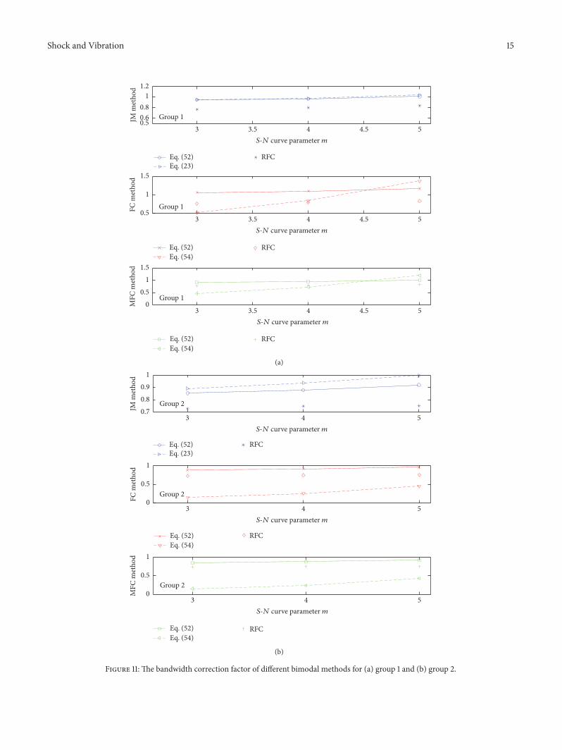

International Journal of
AerospaceEngineeringHindawi Publishing Corporationhttpwwwhindawicom Volume 2014
RoboticsJournal of
Hindawi Publishing Corporationhttpwwwhindawicom Volume 2014
Hindawi Publishing Corporationhttpwwwhindawicom Volume 2014
Active and Passive Electronic Components
Control Scienceand Engineering
Journal of
Hindawi Publishing Corporationhttpwwwhindawicom Volume 2014
International Journal of
RotatingMachinery
Hindawi Publishing Corporationhttpwwwhindawicom Volume 2014
Hindawi Publishing Corporation httpwwwhindawicom
Journal ofEngineeringVolume 2014
Submit your manuscripts athttpswwwhindawicom
VLSI Design
Hindawi Publishing Corporationhttpwwwhindawicom Volume 2014
Hindawi Publishing Corporationhttpwwwhindawicom Volume 2014
Shock and Vibration
Hindawi Publishing Corporationhttpwwwhindawicom Volume 2014
Civil EngineeringAdvances in
Acoustics and VibrationAdvances in
Hindawi Publishing Corporationhttpwwwhindawicom Volume 2014
Hindawi Publishing Corporationhttpwwwhindawicom Volume 2014
Electrical and Computer Engineering
Journal of
Advances inOptoElectronics
Hindawi Publishing Corporation httpwwwhindawicom
Volume 2014
The Scientific World JournalHindawi Publishing Corporation httpwwwhindawicom Volume 2014
SensorsJournal of
Hindawi Publishing Corporationhttpwwwhindawicom Volume 2014
Modelling amp Simulation in EngineeringHindawi Publishing Corporation httpwwwhindawicom Volume 2014
Hindawi Publishing Corporationhttpwwwhindawicom Volume 2014
Chemical EngineeringInternational Journal of Antennas and
Propagation
International Journal of
Hindawi Publishing Corporationhttpwwwhindawicom Volume 2014
Hindawi Publishing Corporationhttpwwwhindawicom Volume 2014
Navigation and Observation
International Journal of
Hindawi Publishing Corporationhttpwwwhindawicom Volume 2014
DistributedSensor Networks
International Journal of