An Analytical Critique of ‘New Keynesian’ …js4pke.jp/pkr/PKR/2013/asada.pdfPost Keynesian Review Vol. 2, No. 1, Pages 1–28 (the 31st August, 2013) ISSN 2187-4875 An Analytical

Post Keynesian ReviewVol. 2, No. 1, Pages 1–28 (the 31st August, 2013)ISSN 2187-4875

An Analytical Critique of ‘New Keynesian’ Dynamic Model

ASADA, Toichiro

ABSTRACT. In this paper, we present an analytical critique of New Keynesian dy-namic model. It is shown analytically that the prototype New Keynesian dynamicmodel produces the paradoxical behaviors that are inconsistent with the empiricalfacts. We also present more traditional alternative approach that is consistent withthe empirical facts, which is called the Old Keynesian dynamic model.

Keywords: New Keynesian dynamic model, (in)determinacy, exogenous disturbance,Old Keynesian dynamic model, (in)stability, Hopf bifurcation, endogenousfluctuation.

JEL Classification: E12, E31, E32, E52

1. Introduction

Recently, the so-called New Keynesian(NK) dynamic model, which is representedby Woodford(2003), Bénassy(2007), Galí(2008) and others, is becoming more andmore influential in the mainstream macroeconomic analysis. The method of mod-eling that is adopted in this approach is based on the dynamic optimization of therepresentative agents with perfect foresight or rational expectations, but it contra-dicts Keynes’(1936) own vision on the working of the market economy that is basedon the bounded rationality due to the inherent fundamental uncertainty.

In this paper, we present an internal and analytical critique of the NK dynamicmodel. The adjectives internal and analytical mean that our critique is based onthe detailed mathematical study of the prototype NK dynamic model. It is shownthat this model produces the paradoxical behaviors of the main variables whichcontradict the empirical facts. We also propose an alternative approach that is calledthe Old Keynesian dynamic model, which is immune from such kind of anomaly.

In Section 2, we formulate the simplest version of the prototype NK dynamicmodel in terms of a linear system of difference equations. In Section 3, we presenta detailed mathematical analysis of such a model without exogenous disturbances.Section 4 is devoted to critical considerations of the prototype NK dynamic model,

Professor Dr. Asada Toichiro, Faculty of Economics, Chuo University, Tokyo, Japan.

©2013 The author and The Japanese Society for Post Keynesian Economics

1

2 ASADA, Toichiro

which is largely based on the analysis in Section 3. Section 5 provides a detailedanalysis of the effects of the exogenous but non-stochastic disturbances in the NKsetting.

The considerations up to Section 5 have rather critical and negative implica-tions, although they are largely based on the detailed mathematical analyses. InSection 6, however, we propose an alternative positive and constructive approach,which is called the Old Keynesian dynamic model in contrast to the NK dynamicmodel. Section 7 is devoted to concluding remarks. Mathematical appendices sup-plement the descriptions in the text.

2. Formulation of the Prototype NK Dynamic Model

The simplest version of the prototype NK dynamic model may be formulated asfollows.1

�t D �etC1 C ˛.yt � Ny/C "t ;(2.1)

yt D yetC1 � ˇ.rt � �e

tC1 � �o/C �t ;(2.2)

rt D �o C N� C 1.�t � N�/C 2.yt � Ny/;(2.3)

�etC1 D Et�tC1; ye

tC1 D EtytC1;(2.4)

where �t the rate of price inflation at period t , �etC1 expected rate of price inflation

at period t C 1, i.e. rate of price inflation at period t C 1 that is expected at periodt , Yt real national income at period t , yt D logYt , Y e

tC1 expected real nationalincome at period t C 1 (real national income at period t C 1 that is expected atperiod t ), ye

tC1 D logY etC1, rt nominal rate of interest at period t , �o equilibrium

value of the real rate of interest (fixed), NY equilibrium value of the real nationalincome (fixed), Ny D log NY , and N� target rate of inflation that is set by the centralbank (fixed). All of the parameter values ˛, ˇ, 1 and 2 are positive. The terms"t and �t represent the (stochastic or non-stochastic) exogenous disturbances. Notethat rt � �e

tC1 expresses the expected real rate of interest at period t .Equations (2.1) and (2.2) represent NK Phillips curve and NK IS curve respec-

tively. According to the NK convention that sticks to the so-called microeconomicfoundation, (2.1) is derived from the optimizing behavior of the imperfectly com-petitive firms with costly price changes, and (2.2) is derived from the first order

1 As for the textbooks of the New Keynesian dynamic model by the original authors, see Wood-ford(2003), Bénassy(2007) and Galí(2008). Romer(2006) contains some useful expositions. Theformulation in this section is the simplified version of the formulation by Asada, Chiarella, Flascheland Proaño(2007). See also Flaschel, Franke and Proaño(2008) and Asada, Chiarella, Flaschel andFranke(2010) as for similar formulations.

The Japanese Society for Post Keynesian Economics

ANALYTICAL CRITIQUE OF NK DYNAMICS 3

condition of the inter-temporal optimization for the representative consumers, thatis called the Euler equation of consumption.2 This means that the real aggregatedemand becomes a decreasing function of the real rate of interest even if the firms’investment expenditure is neglected in this model. (2.3) represents the interest ratemonetary policy rule of the central bank by means of the Taylor rule, which is alsocalled the flexible inflation targeting that considers both of the rate of price infla-tion and the employment(real output).3 (2.4) is the formalization of the rationalexpectation hypothesis concerning the rate of price inflation and the real output.4

We can rewrite equations (2.1) and (2.2) as follows.

�etC1 � �t D ˛. Ny � yt/ � "t ; .˛ > 0/(2.5)

yetC1 � yt D ˇ.rt � �e

tC1 � �o/ � �t ; .ˇ > 0/:(2.6)

Substituting (2.3) into these two equations, we have the following system ofequations.

�etC1 � �t D ˛. Ny � yt/ � "t D F1.yt I "t/;(2.7a)

yetC1 � yt D ˇf. 1 � 1/.�t � N�/C .˛ C 2/.yt � Ny/C "tg � �t(2.7b)

D F2.�t ; yt I "t ; �t/;

�etC1 D Et�tC1; ye

tC1 D EtytC1:(2.7c)

3. Mathematical Analysis of the System without Exogenous Disturbance

The system (2.7) is called the DSGE (Dynamic Stochastic General Equilibrium)model if at least one of the exogenous disturbances "t and �t is a stochastic variable.On the other hand, this system is called DGE (Dynamic General Equilibrium) modelif there is no stochastic disturbance.5 In this section, we shall consider the casewithout exogenous disturbance, that is to say,

(3.1) "t D �t D 0:

In this case, the rational expectation hypothesis, that is expressed by (2.7c) , isreduced to the following perfect foresight hypothesis.

(3.2) �etC1 D �tC1; y

etC1 D ytC1:

2 In fact, these equations are log-linear approximations of the optimal conditions of the economicagents.

3 See Taylor(1993) as for the original formulation of the Taylor rule.4Et stands for the operator of the mathematical expectation.5 See Woodford(2003), Bénassy(2007), Galí(2008), and Chiarella, Flaschel and Semmler(2013).

Post Keynesian Review Vol. 2

4 ASADA, Toichiro

In such a case, equations (2.5) and (2.6) become

��t D �tC1 � �t D ˛. Ny � yt/;(3.3)

�yt D ytC1 � yt D ˇ.rt � �tC1 � �o/;(3.4)

and the system (2.7) becomes as follows.

�tC1 D �t C ˛. Ny � yt/ D G1.�t ; yt/;(3.5a)

ytC1 D yt C ˇf. 1 � 1/.�t � N�/C .˛ C 2/.yt � Ny/g D G2.�t ; yt/:(3.5b)

The equilibrium solution .��; y�/ of this system becomes simply

(3.6) ��D N�; y�

D Ny;

and the Jacobian matrix J1 of this system becomes as follows.

(3.7) J1 D

1 �˛

ˇ. 1 � 1/ 1C ˇ.˛ C 2/

!:

Its characteristic equation is given by

(3.8) '1.�/ � j�I � J1j D �2C a1�C a2 D 0;

where

a1 D � trJ1 D �2 � ˇ.˛ C 2/ < 0;(3.9)

a2 D jJ1j D 1C ˇ.˛ C 2/C ˛ˇ. 1 � 1/ D 1C ˇ.˛ 1 C 2/ > 1:(3.10)

Then, we have the following set of relationships.

A1 � 1C a1 C a2 D ˛ˇ. 1 � 1/;(3.11a)

A2 � 1 � a2 D �ˇ.˛ 1 C 2/ < 0;(3.11b)

A3 � 1 � a1 C a2 D 4C ˛ˇ C 2ˇ 2 C ˛ˇ 1 > 0:(3.11c)

The equilibrium point of the system of difference equations (3.5) is dynamicallystable if and only if j�j j < 1, where �j , j D 1; 2, are two characteristic roots of(3.8). It is well known that such a stability condition is in fact satisfied if and onlyif the following set of inequalities are satisfied.6

(3.12) Aj > 0; j D 1; 2; 3:

In addition, the discriminant of the characteristic roots is given by

(3.13) D � a21 � 4a2 D ˇfˇ.˛ C 2/

2C 4˛.1 � 1/g:

6 See Gandolfo(2009, p.60). The set of inequalities (3.12) is the two-dimensional version of theso-called Schur-Cohn stability conditions of difference equations.



That is to say, the characteristic equation (3.8) has a pair of conjugate complex rootsif and only if D < 0.

Now, we can obtain the following result.

LEMMA 3.1. (1) At least one root of (3.8) has the absolute value that is greaterthan 1 for all 1 > 0. In other words, equilibrium of (3.5) is unstable.(2) The characteristic equation (3.8) has a pair of conjugate complex roots, if and

only if the inequality 1 > 1Cˇ.˛ C 2/

2

4˛is satisfied.

Proof. (1) Inequality (3.11b) means that at least one of the Schur-Cohn stabilityconditions (3.12) is violated.

(2) It follows from (3.13) that we have D < 0 if and only if the inequality

1 > 1Cˇ.˛ C 2/

2

4˛is satisfied. □

The equilibrium point of the system (3.5) is called totally unstable if and onlyif both of two roots of (3.8) have the absolute values that are greater than 1.

In what follows, we write

� Dˇ.˛ C 2/

2

4˛:

To study whether the system is totally unstable or not, it is convenient to con-sider the inverse matrix of J1, that is,

(3.14) K � J1�1

D1

1C ˇ.˛ 1 C 2/

1C ˇ.˛ C 2/ ˛

ˇ.1 � 1/ 1

!:

Then, let us consider the following characteristic equation.

(3.15) .�/ � j�I �Kj D �2C b1�C b2 D 0;

where

b1 D � trK D�2 � ˇ.˛ C 2/

1C ˇ.˛ 1 C 2/< 0:(3.16)

b2 D jKj D1

1C ˇ.˛ 1 C 2/< 1:(3.17)

Therefore, we obtain the following relationships.

B1 � 1C b1 C b2 Dˇ˛. 1 � 1/

1C ˇ.˛ 1 C 2/;(3.18a)

B2 � 1 � b2 Dˇ.˛ 1 C 2/

1C ˇ.˛ 1 C 2/> 0;(3.18b)

B3 � 1 � b1 C b2 D4C ˇf˛.1C 1/C 2 2g

1C ˇ.˛ 1 C 2/> 0:(3.18c)


6 ASADA, Toichiro

The following lemma is a direct consequence of the relationships (3.18).

LEMMA 3.2. Absolute values of all of two roots of (3.8) are greater than 1, if andonly if 1 > 1. In other words, the equilibrium point of (3.5) is totally unstable ifand only if 1 > 1.

Proof. It follows from the Schur-Cohn stability condition with respect to the systemof difference equations that we have a set of inequalities with respect to (3.18)

(3.19) Bj > 0; .j D 1; 2; 3/

if and only if 1 > 1. (Cf. Footnote 6). This means that all of the absolute valuesof the roots of the characteristic equation (3.15) are less than 1 if and only if 1 > 1.This result together with Theorem A.1 in Appendix A implies Lemma 3.2. □

Lemmas 3.1 and 3.2 entail the following proposition.

PROPOSITION 3.1. Let �1 and �2 stand for two roots of (3.8).(1) If 0 < 1 < 1, then �1 and �2 are real with 0 < �1 < 1 < �2. In this case, theequilibrium of (3.5) becomes a saddle point.(2) If 1 D 1, then �1 and �2 are real, with �1 D 1 < �2.(3) If 1 < 1 < 1 C �, then �1 and �2 are real, with 1 < �1 < �2. In this case,the equilibrium of (3.5) becomes totally unstable, and any solution path that startsfrom points off equilibrium diverges monotonically.(4) If 1 D 1C �, then two roots are duplicated such that 1 < �1 D �2.(5) If 1 C � < 1 , then the two roots are a pair of conjugate complex roots suchthat j�1j D j�2j D

p�2 C !2 > 1, where �1 D � C i!; �2 D � � i!, ! 6D 0 and

i Dp

�1. In this case, the equilibrium of (3.5) becomes totally unstable, and anysolution path that starts from points off equilibrium diverges cyclically.

As for proof, see Appendix B.

4. Some Critical Assessments

The prototype NK dynamic model that was taken up in the previous sections hasseveral problematical features. In this section, we shall try to provide some criticalassessments of such a model.

4.1. Anomalous dynamics with sign reversals. The most notorious problem ofthe prototype NK dynamic model is the phenomenon that is called the sign reversalin New Keynesian Phillips curve, pointed out by Mankiw (2001) clearly.7

7 As for the related topics, see also Asada, Chiarella, Flaschel and Franke(2010), Flaschel andSchlicit(2006), Franke(2007) and Romer(2006).



It follows from (3.3) that��t becomes a decreasing function of yt . That is, therate of price inflation continues to decrease whenever the actual real output level isgreater than the natural real output level. This contradicts the empirical fact of themost of countries. Mankiw(2001) writes as follows.

“Although the New Keynesian Phillips curve has many virtues, italso has one striking vice: It is completely odds with the facts. Inparticular, it cannot come even close to explaining the dynamic ef-fects of monetary policy on inflation and unemployment. This harshconclusion shows up several places in the recent literature, but judg-ing from the continued popularity of this model, I think it is fairto say that its fundamental inconsistency with the facts is not veryappreciated.” (Mankiw, 2001, p. C52)

It is worth noting that there is another difficulty of sign reversal in this model,which Mankiw(2001) does not refer to. That is, it follows from (3.4) that �yt be-comes an increasing function of rt � �tC1. This means that the real output levelcontinues to increase whenever the actual real interest rate is greater than its equi-librium level. It is evident that this fact also contradicts the empirical fact of themost of countries.

4.2. Problematical jump variable technique. In the traditional economic dy-namic models, that conforms with the orthodox mathematical concept of stability,the initial values of the endogenous variables are historically given. In this setting,the equilibrium point is considered to be stable if and only if all of the characteristicroots are stable roots, and it is considered to be unstable if at least one characteris-tic root is an unstable root.8 Lemma 3.1(1) means that the prototype NK model isaccompanied by equilibrium that is unstable in the mathematically orthodox sense.The equilibrium of NK dynamic model will never be reached. This underminesthe basis of the NK theory, however. Hence, the NK literature adopts the trick thatmakes the unstable system try to mimic a ‘stable’ system by using the so-calledjump variable technique.

In the NK dynamic model, both of two endogenous variables �t and yt areconsidered to be jump variables or not-predetermined variables, the initial valuesof which are freely chosen by the economic agents. Furthermore, it is assumed that

8A stable (resp. unstable) root is the root which has the absolute value that is less (resp. greater)than 1 in case of the system of difference equations, and it is the root which has the negative (resp.positive) real part in case of the system of differential equations.


8 ASADA, Toichiro

by the economic agents only the initial conditions of the endogenous variables arechosen so as to ensure the convergence to the equilibrium point.9

Hence, in place of the concept of stability and instability, NK literature intro-duces the following concept of the determinacy and indeterminacy.10

DEFINITION 4.1. (1) Suppose that a set of the initial values of the jump variables,which ensures the convergence to the equilibrium point, is uniquely determined.Then, the system is called determinate.

(2) Suppose that there are multiple sets of the initial values of the jump vari-ables which ensure the convergence to the equilibrium point. Then, the system iscalled indeterminate.

PROPOSITION 4.1. (1) If 0 < 1 < 1, then the system (3.5) is indeterminate.(2) If 1 < 1, the system (3.5) is determinate.

The meanings of Proposition 4.1 are as follows.The general solution of the system of difference equations (3.5) becomes

(4.1)

�t

yt

!D

2Xj D1

Cj

Dj

!�t

j C

N�

Ny

!;

where the constants Cj and Dj must satisfy the following relationships

(4.2)

�j � 1 ˛

�ˇ. 1 � 1/ �j � f1C ˇ.˛ C 2/g

! Cj

Dj

!D

0

0

!; .j D 1; 2/:

(See Gandolfo, 2009, Ch.5). Substituting (4.2) into (4.1) we obtain

(4.3)

�t

yt

!D

1

1��1

˛

!C1�

t1 C

1

1��2

˛

!C2�

t2 C

N�

Ny

!;

where constants C1 and C2 are determined by a set of initial values in the followingway.

�o D C1 C C2 C N�;(4.4a)

yo D1 � �1

˛C1 C

1 � �2

˛C2 C Ny:(4.4b)

First, suppose that 0 < 1 < 1. In this case, we can consider that �1 and �2 arereal values such that 0 < �1 < 1 and 1 < �2 without loss of generality in view of

9 Usually, this assumption is rationalized on the ground that the transversality condition, thatrequires the convergence to the equilibrium point, must be satisfied in order to ensure the behaviorof the representative agents to be truly optimal.

10 See Woodford(2003), Bénassy(2007), and Galí(2008). See Blanchard and Kahn(1980) as forthe sophisticated mathematical treatment that is related to this concept.



-

6

0 yt

�t

Nyr

N� r Er�

�

A

B

FIGURE 1. Case of 0 < 1 < 1 (Indeterminate).

Proposition 3.1(1). In this situation, only the pair of the initial values .�o; yo/ thatsatisfies the condition C2 D 0 can ensure the convergence to the equilibrium point.This condition is reduced to the following set of equations in view of (4.4).

�o D C1 C N�;(4.5a)

yo D1 � �1

˛C1 C Ny:(4.5b)

Substituting (4.5b) into (4.5a), we obtain the following relationship between �o

and yo that ensures the convergence to the equilibrium point.

(4.6) �o � N� D˛

1 � �1

.yo � Ny/; 0 < �1 < 1:

Any pair .�o; yo/ that is on the line in Figure 1 satisfies the relationship (4.6).Therefore, there are infinite numbers of the pairs of the initial values .�o; yo/ whichensure the convergence to the equilibrium point.11 In other words, the system be-comes indeterminate in case of 0 < 1 < 1.

Next, suppose that 1 > 1. In this case, both of the absolute values of �1 and �2

become greater than 1 (see Lemma 3.2). In this situation, only the pair of the initialvalues .�o; yo/ that satisfies the condition C1 D C2 D 0 can ensure the convergence

11 In fact, the line in Figure 1 is the saddle path.


10 ASADA, Toichiro

-

6

0 yt

�t

Nyr

N� r Er

FIGURE 2. Case of 1 > 1 (Determinate).

to the equilibrium point. Substituting this condition into (4.4), we obtain

(4.7) �o D N�; yo D Ny:

This means that the system is determinate in case of 1 > 1, but in this case,the economic agents in this model select only the solution that is stuck to the equi-librium point E in Figure 2 for all times. In this case, the economic fluctuationdoes not occur unless there are exogenous disturbances, and the dynamic model isreduced to the static model virtually.

We think that the adoption of such a jump variable technique in the NK dynamicmodel is unconvincing because of the following three reasons.

Firstly, as Mankiw(2001) pointed out, actual economic data suggest that the rateof price inflation is not the jump variable that conveniently jumps discontinuously,but it is a state variable that moves sluggishly. Mankiw(2001) writes as follows.

“In these models of staggered price adjustment, the price level ad-justs slowly, but the inflation rate jumps quickly. Unfortunately forthe model, that is not what we see in the data.” (Mankiw, 2001, p.C54)

A proposal to resolve such a problem is to introduce the inertia into the modelby considering the backward-looking factors. Typical method of reformulation isto replace (2.1) by the following new equation that includes the backward-looking



factor �t�1 as well as the forward-looking factor �etC1.12

(4.8) �t D ��etC1 C .1 � �/�t�1 C ˛.yt � Ny/C "t ; 0 < � < 1:

However, such a reformulation is rather ad hoc and it is not clear how it can bederived from the analytical framework of the NK dynamic model consistently.

Secondly, as we already pointed out, the prototype NK dynamic model cannotproduce the economic fluctuations unless we introduce the exogenous disturbancesinto the model. This conclusion is not confined to the case of determinacy (the caseof 1 > 1). It also applies to the case of indeterminacy (the case of 0 < 1 < 1),because even in case of indeterminacy, the solution converges to the equilibriumpoint monotonically (see Figures 1 and 2). In other words, the endogenous eco-nomic fluctuation is impossible in this model.

Thirdly, some economists criticize the methodology of the representative agentapproach of the NK dynamic model that is based on the analysis of the behav-ior of the omniscient and homogeneous representative agent. For example, Kir-man(1992), Asada, Chiarella, Flaschel and Franke(2010) and Chiarella, Flascheland Semmler(2013) proposed the approach that considers the interactions of theheterogeneous agents who behave bounded-rationally.13 Let us quote from theirpapers.

“A tentative conclusion, at this point, would be that the representa-tive agent approach is fatally flawed because it attempts to imposeorder on the economy through the concept of an omniscient individ-ual. In reality, individuals operate in very small subsets of the econ-omy and interact with those with whom they have dealings. It maywell be that out of this local but interacting activity emerges somesort of self organization which provides regularity at the macroeco-nomic level. � � � � � � The equilibria of the worlds described by anyof these approaches may be conceptually very different from thoseimplied by the artifact of the representative individual. Cycles andfluctuations emerge not as the result of some substantial exogenousshock and the reaction to it of one individual, but as a natural resultof interaction, together with occasional small changes or ‘mutations’in the behavior of some individuals.” (Kirman, 1992, pp.132-3)

12 See, for example, Furler(1997). Romer(2006, Ch.6) and Franke(2007) contain the usefulinterpretations of this topic.

13 Such an approach is somewhat similar to the approach of Akerlof and Shillar(2009) that isinfluenced by the discourse of Keynes(1936).


12 ASADA, Toichiro

“While the microfoundation of economic behavior is per se an im-portant desideratum to be reflected also by behaviorally orientedmacrodynamics, the use of ‘representative’ consumers and firms forthe explanation of macroeconomic phenomena is too simplistic andalso too narrow for a proper treatment of what is really interestingon the economic behavior of economic agents – the interaction ofheterogeneous agents –, and it is also not detailed enough to dis-cuss the various feedback channels present in the real world. � � � � � �

Indeed, agents are heterogeneous, form heterogeneous expectationsalong other lines than suggested by the rational expectations theory,and have different short and long term views about the economy.”(Asada, Chiarella, Flaschel and Franke, 2010, pp.205-6)

“Central to our approach is the use of non-market clearing adjust-ment process that are indeed the basis for the consideration of thevarious Keynesian macroeconomic feedback effect, the Pigou realbalance effect, the Tobin price expectation effect (where an expectedprice fall will trigger instabilities), and the Keynes effect in the con-text of a dynamic multiplier model. These have all been character-istic in the traditional Keynesian approaches to macrodynamics buthave mostly been forgotten in modern macroeconomics.” (Chiarella,Flaschel and Semmler, 2013, p.110)

5. Mathematical Analysis of the Effects of the Exogenous Disturbance in aPrototype New Keynesian Dynamic Model

In this section, we introduce the exogenous disturbance into the model and study itseffects mathematically.14 In (2.7), we assume that "t D 0 and �t are exogenousbut non-stochastic disturbances, that is,

�tC1 D �t C ˛. Ny � yt/;(5.1a)

ytC1 D yt C ˇf. 1 � 1/.�t � N�/C .˛ C 2/.yt � Ny/g � �t :(5.1b)

Furthermore, let us assume as follows.

(5.2) For all t 2 f0; 1; 2; : : : ; to � 1g; �t D N�; yt D Ny:

14 As we see in this section, the existence of the exogenous disturbance is essential for the occur-rence of the economic fluctuations in the prototype NK dynamic model, but the stochastic elementdoes not play the essential role.



�t D

8̂̂<̂:̂0 for t 2 f0; 1; 2; : : : ; to � 1g,

�to6D 0 for t D to,

�to�.t�to/ for t 2 fto C 1; to C 2; : : :g,

(5.3)

where �tois given, and 0 < � < 1.

Then, we have the following three-dimensional system of difference equationsfor all time periods t 2 fto; to C 1; : : :g:

�tC1 D �t C ˛. Ny � yt/ D G1.�t ; yt/;(5.4a)

ytC1 D yt C ˇf. 1 � 1/.�t � N�/C .˛ C 2/.yt � Ny/g � �t(5.4b)

D G2.�t ; yt ; �t/;

�tC1 D ��t :(5.4c)

The Jacobian matrix of this system becomes

(5.5) J2 D

0B@ 1 �˛ 0

ˇ. 1 � 1/ 1C ˇ.˛ C 2/ �1

0 0 �

1CA ;and the characteristic equation of this system is given by

(5.6) '2.�/ � j�I � J2j D j�I � J1j.� � �/ D 0;

where J1 is defined by (3.7).This characteristic equation has a real root �3 D � and other two roots are

determined by (3.8). To simplify the analysis, we consider only the case of

(5.7) 1 < 1 < 1C �:

It follows from Proposition 3.1(3) that (3.8) has two real roots such that 1 <�1 < �2. In this case, the general solution of (5.4) for t � to becomes

(5.8)

0B@�t

yt

�t

1CA D

3Xj D1

0B@Cj

Dj

Ej

1CA�tj C

0B@ N�

Ny

0

1CA ;where 1 < �1 < �2, 0 < � < 1, and the relationships that, for j D 1; 2; 3,

(5.9)

0B@ �j � 1 ˛ 0

�ˇ. 1 � 1/ �j � f1C ˇ.˛ C 2/g 1

0 0 �j � �

1CA0B@Cj

Dj

Dj

1CA D

0B@000

1CA ;must be satisfied (see Gandolfo, 2009, Ch.9).


14 ASADA, Toichiro

Rewriting (5.8) by using (5.9), we obtain the following relationship.

(5.10)

0B@�t

yt

�t

1CA D

0B@ 11��1

˛

0

1CAC1�t�to

1 C

0B@ 11��2

˛

0

1CAC2�t�to

2 C

0B@ ˛�

1��

1

1CAE3�t�to C

0B@ N�

Ny

0

1CA ;where

� D ˛ˇ. 1 � 1/C .1 � �/f1C ˇ.˛ C 2/ � �g > 0;

and C1; C2 and E3 are the constants which are determined by the initial values.�to

; yto; �to

/. In fact, we have the following relationships from (5.10).

�toD C1 C C2 C

˛

��to

C N�;(5.11a)

ytoD1 � �1

˛C1 C

1 � �2

˛C2 C

1 � �

��to

C Ny;(5.11b)

�toD E3:(5.11c)

We can determine the values of C1; C2 and E3 by solving (5.11) if a triplet of theinitial values .�to

; yto; �to

/ is predetermined. However, in the NK setting, the initialvalues �to

and ytoare considered to be not-predetermined variables which can be

chosen freely by the economic agents, although the initial value of the exogenousdisturbance .�to

/ is a predetermined variable.Furthermore, it is assumed that the economic agents choose only the pair of

the initial values .�to; yto

/ which ensures that the solution (5.10) converges to theequilibrium point . N�; Ny/. It is apparent that only the initial values that satisfy thecondition

(5.12) C1 D C2 D 0

can ensure the convergence to the equilibrium point. Substituting (5.12) into (5.11),we obtain the following requirement.

�toD˛

��to

C N�;(5.13a)

ytoD1 � �

��to

C Ny:(5.13b)

From the assumptions 1 > 1, 0 < � < 1 and (5.13), we have the relationships

(5.14) sign.�to� N�/ D sign.yto

� Ny/ D sign �to;



and the special solution that ensures the convergence to the equilibrium point be-comes as follows.

�t D˛

��to�t�to C N�;(5.15a)

yt D1 � �

��to�t�to C Ny;(5.15b)

�t D �to�t�to :(5.15c)

Figure 3 is the so-called impulse response functions that are produced by thespecial solution (5.15) in case of �to

< 0. In this figure, it is supposed that thesystem is at the equilibrium point for 0 � t < to, the exogenous disturbance iscaused at the time period t D to, and then it diminishes continuously. Respondingto this exogenous disturbance, the pair of the values of � and y suddenly jumps tothe initial condition .�to

; yto/ that ensures the convergence to the equilibrium point

conveniently. The jump variable postulate manages to conceal the paradoxicalbehavior of the main variables.

However, it is not clear why the economic agents in this model can choose thespecial initial values that are given by (5.13) immediately after the exogenous shockoccurs. What occurs if another combination of the initial conditions is chosen bymistake?

As a thought experiment, let us assume that

(5.16) �toD N�; yto

D Ny;

even if �to6D 0, which means that the economic variables cannot conveniently

jump even if an exogenous shock occurs.Substituting (5.16) into (5.11), we have the following system of equations.

(5.17)

1 1

1��1

˛1��2

˛

! C1

C2

!D �

�to

�

˛

1 � �

!:

Solving this equation with respect to C1 and C2, we obtain the following result.

C1 D�˛.�2 � �/

.�2 � �1/��to;(5.18a)

C2 D˛.�1 � �/

.�2 � �1/��to:(5.18b)

Substituting (5.18) and E3 D �tointo (5.10), we obtain the special solution of the

system when (5.16) is assumed.Since it is assumed that 0 < � < 1 < �1 < �2, (5.18) implies that

(5.19) � signC1 D signC2 D sign �to:


16 ASADA, Toichiro

-

6

(a) 0 t

�t

bto

rr�to

-

6

(b) 0 t

�t

bto

r

r

�to

N�

-

6

(c)

0 t

yt

b

to

r

r

yto

FIGURE 3. The special solution (5.15) in case of �to< 0.



-

6

(a) 0 t

�t

bto

rr�to

-

6

(b) 0 t

�t

rtob

rN�

-

6

(c)

0 t

yt

bto

rrNy

FIGURE 4. The special solution (5.10) in case of �toD N�; yto

D

Ny; �to< 0.


18 ASADA, Toichiro

In this case, the propagation process of the effects of the exogenous disturbancebecomes as follows. For simplicity, we consider only the case of �to

< 0.If (5.16) is satisfied, we have the following from (5.4) in case of �to

< 0.

�toC1 D N� D �to;(5.20a)

ytoC1 D Ny � �to> Ny D yto

;(5.20b)

�toC2 D N� C ˛. Ny � ytoC1/ D N� C ˛�to< N� D �toC1;(5.20c)

ytoC2 D ytoC1 C .˛ C 2/.ytoC1 � Ny/ D ytoC1 � .˛ C 2/�to> ytoC1:(5.20d)

A set of relationships (5.20) means that the fall of � and the rise of y are causedsoon after this exogenous shock. This tendency is not restricted to the periods soonafter the shock.

We have C1 > 0; C2 < 0 and 1 < �1 < �2 where �2 is the dominant root thatgoverns the dynamic behavior of the system in case of C2 6D 0. Therefore, (5.10)implies that � continues to fall and y continues to rise ultimately, which meansthat the deflationary prosperity rather than the deflationary depression is caused bythis exogenous shock. Figure 4 illustrates the typical impulse response functions ofsuch unconvincing and paradoxical behaviors of the main variables that are causedby the exogenous disturbance.

6. Toward an Alternative Old Keynesian Approach

Up to the previous section, we presented an analytical critique of the prototype NKdynamic model. The point is that the prototype NK dynamic model produces theanomalous behaviors that are inconsistent with the empirical facts.

In this section, we develop a constructive and alternative approach that waspresented by Asada(2012), which is called the Old Keynesian dynamic model afterTobin(1969, 1994).15

Asada’s(2012) Old Keynesian dynamic model consists of the following set ofequations.16

�t D xt C f .yt/ ; f . Ny/ D 0; fy D f 0.yt/ > 0;(6.1)

yt D zt C g.rt � xt/ ; gr�x D g0.rt � xt/ < 0;(6.2)

xt D �etC1; zt D ye

tC1;(6.3)

15 The work, such as Asada, Chiarella, Flaschel and Franke(2003, 2010), Chiarella, Flaschel andFranke(2005), and Asada, Flaschel, Mouakil and Proanõ(2011), is also based on the Old Keynesiantradition of the modeling methodology.

16 In this formulation, the exogenous disturbance is neglected for simplicity.



�rt D rtC1 � rt D

( 1.�t � N�/C 2.yt � Ny/; if rt > 0;

maxŒ0; 1.�t � N�/C 2.yt � Ny/�; if rt D 0;(6.4)

�xt D xtC1 � xt D ıŒ�1. N� � xt/C .1 � �1/.�t � xt/�; 0 � �1 � 1;(6.5)

�zt D ztC1 � zt D �Œ�2. Ny � zt/C .1 � �2/.yt � zt/�; 0 � �2 � 1;(6.6)

where xt stands for the expected rate of price inflation, zt the expected real nationalincome, and rt � xt the expected real interest rate; 1; 2; ı and � are positive pa-rameters. Meanings of other symbols are the same as those in the previous sections;

Equations (6.1) and (6.2) are the expectation-augmented Phillips curve and theexpectation-augmented IS curve respectively. In these formulations, it is allowedfor that the functions f .yt/ and g.rt � xt/ are nonlinear functions.17 (6.4) is aTaylor-rule-type interest rate monetary policy rule. In this formulation, the naturalnonlinearity that is due to the nonnegative constraint of the nominal interest rate isexplicitly considered. Equations (6.5) and (6.6) are the expectation formation equa-tions concerning the rate of price inflation and the real national income. They are themixtures of the forward-looking and backward-looking (adaptive) expectation for-mations, although they are different from the NK rational expectation formations.We can consider that �1 is the parameter that reflects the credibility of the centralbank’s inflation targeting, and �2 is the parameter that reflects the credibility of thecentral bank’s employment targeting. We can consider that the formulations (6.5)and (6.6) are the simplest versions of the heterogeneous expectation hypothesis.

Incidentally, we have the following equations by substituting (6.1) and (6.2)into (6.5) and (6.6).

�xt D ıŒ�1. N� � xt/C .1 � �1/f .yt//�; f0.yt/ > 0;(6.7)

�zt D �Œ�2. Ny � zt/C .1 � �2/g.rt � xt/�; g0.rt � xt/ < 0:(6.8)

These equations imply that the rate of change of the expected rate of inflation�xt isan increasing function of the actual real national income .yt/ and the rate of changeof the expected real national income �zt is a decreasing function of the expectedreal interest rate .rt � xt/. In other words, this Old Keynesian dynamic model isimmune from the notorious NK sign reversal problems.

Asada(2012) showed that this system can be reduced to the following threedimensional system of nonlinear difference equations. First, put

� D 1fxt C f .zt C g.rt � xt// � N�g C 2fzt C g.rt � xt/ � Nyg;

17 The empirical data of the Japanese economy suggests that fyy D f 00.yt / > 0.


20 ASADA, Toichiro

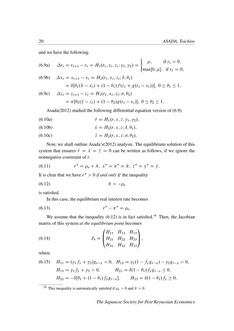
and we have the following.

�rt D rtC1 � rt D H1.rt ; xt ; zt I 1; 2/ D

(�; if rt > 0;

maxŒ0; ��; if rt D 0;(6.9a)

�xt D xtC1 � xt D H2.rt ; xt ; zt I ı; �1/(6.9b)

D ıŒ�1. N� � xt/C .1 � �1/f .zt C g.rt � xt//�; 0 � �1 � 1;

�zt D ztC1 � zt D H3.rt ; xt ; zt I �; �2/(6.9c)

D �Œ�2. Ny � zt/C .1 � �2/g.rt � xt/�; 0 � �2 � 1:

Asada(2012) studied the following differential equation version of (6.9).

Pr D H1.r; x; zI 1; 2/;(6.10a)

Px D H2.r; x; zI ı; �1/;(6.10b)

Pz D H3.r; x; zI �; �2/:(6.10c)

Now, we shall outline Asada’s(2012) analysis. The equilibrium solution of thissystem that ensures Pr D Px D Pz D 0 can be written as follows, if we ignore thenonnegative constraint of r .

(6.11) r�D �o C N�; x�

D ��D N�; z�

D y�D Ny:

It is clear that we have r� > 0 if and only if the inequality

(6.12) N� > ��o

is satisfied.In this case, the equilibrium real interest rate becomes

(6.13) r��

D �o:

We assume that the inequality (6.12) is in fact satisfied.18 Then, the Jacobianmatrix of this system at the equilibrium point becomes

(6.14) J3 D

0B@H11 H12 H13

H21 H22 H23

H31 H32 H33

1CA ;where

H11 D . 1fy C 2/gr�x < 0; H12 D 1.1 � fygr�x/ � 2gr�x > 0;(6.15)

H13 D 1fy C 2 > 0; H21 D ı.1 � �1/fygr�x � 0;

H22 D �ıŒ�1 C .1 � �1/fygr�x�; H23 D ı.1 � �1/fy � 0;

18 This inequality is automatically satisfied if �o > 0 and N� > 0.



H31 D �.1 � �2/gr�x � 0; H32 D �˛�.1 � �2/gr�x � 0;

H33 D ��2 � 0:

The characteristic equation of this system at the equilibrium point becomes asfollows.

(6.16) '3.�/ � j�I � J3j D �3C d1�

2C d2�C d3 D 0;

where

d1 D � trJ3 D �H11 �H22 �H33;(6.17a)

d2 D

ˇ̌̌̌ˇH11 H12

H21 H22

ˇ̌̌̌ˇC

ˇ̌̌̌ˇH11 H13

H31 H33

ˇ̌̌̌ˇC

ˇ̌̌̌ˇH22 H23

H32 H33

ˇ̌̌̌ˇ ;(6.17b)

d3 D �jJ3j > 0; if 0 � �1 < 1 and 0 � �2 < 1:(6.17c)

In this Old Keynesian model, the traditional concept of (in)stability is adopted. Inother words, the jump variables are not allowed for in this model, and the equi-librium point is considered to be locally stable if and only if all of the roots ofthe characteristic equation (6.16) have negative real parts.19 It is well known thatsuch local stability condition is satisfied if and only if the following Routh-Hurwitzconditions are satisfied (see Gandolfo, 2009, Ch.16).

(6.18) dj > 0 .j D 1; 2; 3/; and d1d2 � d3 > 0:

By utilizing this result, Asada(2012) proved the following two propositions.

PROPOSITION 6.1. Suppose that the parameters 1 and 2 are fixed at any positivevalues. Then, the equilibrium point of (6.10) is unstable if either of the followingtwo conditions (a) or (b) is satisfied.

(a) ı > 0 is sufficiently large and �1 is sufficiently small (close to zero).(b) The condition 0 � �1 < 1 is satisfied, ı > 0 and � > 0 are sufficiently large,and �2 is sufficiently small (close to zero).

PROPOSITION 6.2. (1) Suppose that the parameters 1, 2, ı and � are fixed at anypositive values. The equilibrium point of (6.10) is locally asymptotically stable, ifboth of �1 and �2 are close to 1 (including the cases of �1 D 1 and �2 D 1).(2) Suppose that the parameter values ı; �; �1 and �2 are fixed at any values suchthat ı > 0; � > 0; 0 � �1 < 1, and 0 � �2 < 1. Then, the equilibrium point of(6.10) is locally asymptotically stable, if either of 1 > 0 or 2 > 0 is sufficientlylarge.

19 The same traditional concept of stability/instability is adopted also in Post Keynesian literature,such as Keen(2000), Asada(2001), and Charles(2008).


22 ASADA, Toichiro

These two propositions show that the increases (resp. decreases) of the param-eter values �1; �2; 1 and 2 have the stabilizing (resp. destabilizing) effects in thetraditional sense in this Old Keynesian model. In other words, the equilibrium pointof the dynamic system (6.10) is stable (resp. unstable) if the credibility of the infla-tion targeting and the employment targeting by the central bank is high (resp. low)and the central bank’s monetary policy is active (resp. inactive).

Let us select one of such parameters, for example, �1 as a bifurcation parameter,and suppose that the equilibrium point of the system is unstable for all sufficientlysmall values of �1, and it is locally stable for all values of �1 that are sufficientlyclose to 1. Then, there exists at least one bifurcation point �o

1 2 .0; 1/ at which thediscontinuous switch from the unstable system to the stable system occurs as theparameter value �1 increases.

It is apparent that at least one real part of the roots of the characteristic equation(6.16) must be zero at the bifurcation point. However, we cannot have the real root� D 0 at such a bifurcation point, because we have

(6.19) '3.0/ D d3 6D 0; if 0 � �1 < 1 and 0 � �2 < 1

from equations (6.16) and (6.17c). This means that the characteristic equation (6.16)has a pair of pure imaginary roots at the bifurcation point. This situation is enoughto apply the Hopf bifurcation theorem (Appendix C) to the dynamic system (6.10),and we have the following proposition.

PROPOSITION 6.3. The bifurcation point of the dynamic system (6.10), which isthe point at which the discontinuous switch from the unstable system to the stablesystem occurs as one of the parameter values �1; �2; 1 and 2 increases, is in factthe Hopf bifurcation point. In other words, the non-constant closed orbits exist atsome range of the parameter values that are sufficiently close to the bifurcationpoint.

Proposition 6.3 shows that the endogenous cyclical fluctuations occur at somerange of intermediate values of the parameters �1; �2; 1 and 2, even if there is noexogenous disturbance, contrary to the prototype NK dynamic model that cannotproduce the economic fluctuations without the exogenous disturbance.

7. Concluding Remarks

In this paper, we showed that the prototype New Keynesian(NK) dynamic modelproduces several paradoxical and anomalous behaviors, which are inconsistent withthe empirical facts. Sign reversals of NK Philips curve and NK IS curve are typ-ical examples of such anomaly. We also observed that the problematical trick of



the jump variable technique is an unconvincing device. Finally, we presented theoutline of the alternative Old Keynesian dynamic model that is consistent with theempirical facts and immune from the NK anomalies.

Appendix A. The Total Instability Theorem

The following purely mathematical result is useful for the proof of Lemma 3.2 inthe text.

THEOREM A.1. Let A be an n � n matrix with the property jAj 6D 0. Then, theabsolute values of all roots of the characteristic equation j�I �Aj D 0 are greaterthan 1 if and only if the absolute values of all roots of the characteristic equationj�I � A�1j D 0 are less than 1.

Proof. The assumption jAj 6D 0 means that 0 cannot be a characteristic root of theequation j�I � Aj D 0. Let �

A6D 0 be a characteristic root of this equation that

satisfies j�AI � Aj D 0. Then, �I � A D .�A�1 � I /A D �I.A�1 � ��1I /A,

so that j�I � Aj D .�1/n�nj��1I � A�1jjAj: Hence, j�I � Aj D 0 if and only ifj��1I � A�1j D 0.

This means that �B

�1

�A

is a characteristic root of the equation j�I �Bj D 0,

where B � A�1.Suppose that �

Ais a real number. In this case, it is obvious that j�

Aj > 1 if and

only if j�B

j < 1.Next, suppose that �

Ais a complex number such that �

AD � C i!; i D

p�1; ! 6D 0: Then, we have �

BD

1

� C i!D

� � i!

�2 C !2. In this case, we have

j�Aj D

p�2 C !2 and j�

Bj D

1p�2 C !2

. This means that j�Aj > 1 if and only if

j�B

j < 1 even if �A

is a complex number. □

Appendix B. Proof of Proposition 3.1.

The characteristic equation (3.8) has the following properties.

(B.1) ' 01.�/ D 2�C a1,

(B.2) '1.0/ D a2 > 0,(B.3) ' 0

1.0/ D a1 < 0,(B.4) '1.1/ D 1C a1 C a2 D ˛ˇ. 1 � 1/,(B.5) ' 0

1.1/ D 2C a1 D �ˇ.˛ C 2/ < 0.

These properties entail that the following statements hold.


24 ASADA, Toichiro

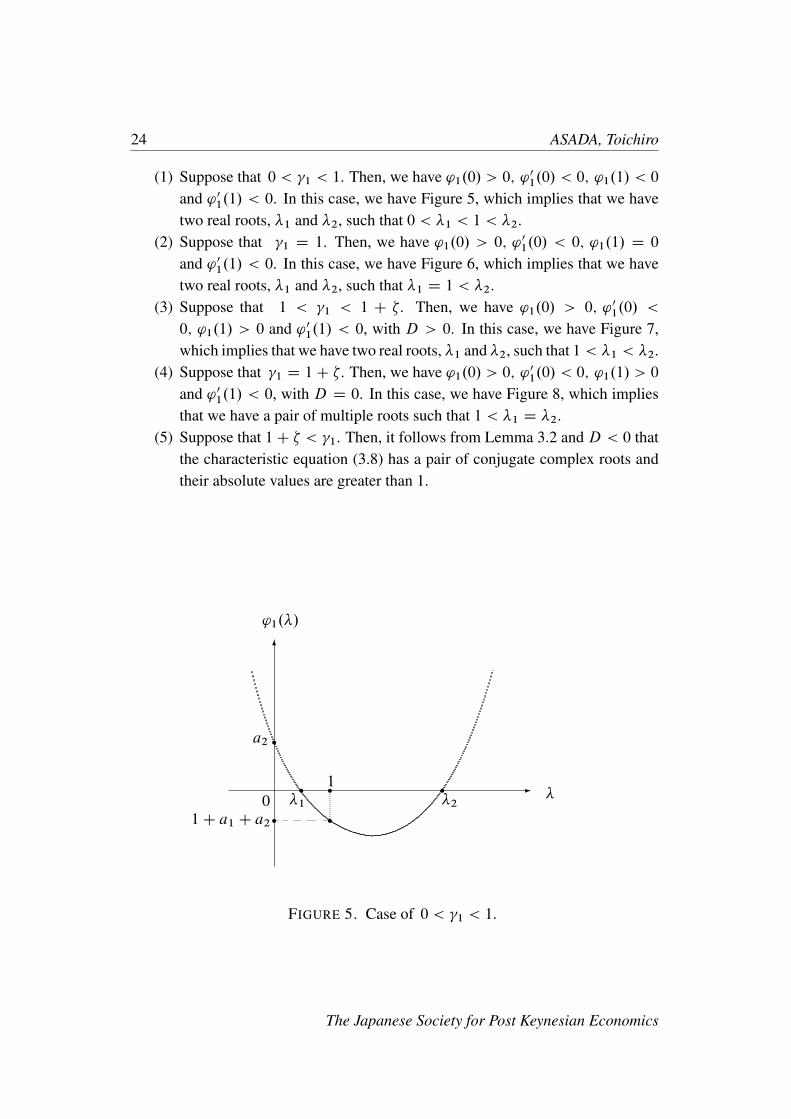
(1) Suppose that 0 < 1 < 1. Then, we have '1.0/ > 0; '01.0/ < 0; '1.1/ < 0

and ' 01.1/ < 0. In this case, we have Figure 5, which implies that we have

two real roots, �1 and �2, such that 0 < �1 < 1 < �2.(2) Suppose that 1 D 1. Then, we have '1.0/ > 0; ' 0

1.0/ < 0; '1.1/ D 0

and ' 01.1/ < 0. In this case, we have Figure 6, which implies that we have

two real roots, �1 and �2, such that �1 D 1 < �2.(3) Suppose that 1 < 1 < 1 C �. Then, we have '1.0/ > 0; ' 0

1.0/ <

0; '1.1/ > 0 and ' 01.1/ < 0, with D > 0. In this case, we have Figure 7,

which implies that we have two real roots, �1 and �2, such that 1 < �1 < �2.(4) Suppose that 1 D 1C �. Then, we have '1.0/ > 0; '

01.0/ < 0; '1.1/ > 0

and ' 01.1/ < 0, with D D 0. In this case, we have Figure 8, which implies

that we have a pair of multiple roots such that 1 < �1 D �2.(5) Suppose that 1C � < 1. Then, it follows from Lemma 3.2 and D < 0 that

the characteristic equation (3.8) has a pair of conjugate complex roots andtheir absolute values are greater than 1.

-

6

0 �

'1.�/

r

a2 r1r

�1

r�2

r1C a1 C a2

r

FIGURE 5. Case of 0 < 1 < 1.



-

6

0 �

'1.�/

a2r

1r�1 �2

r

FIGURE 6. Case of 1 D 1.

-

6

0 �

'1.�/

r

a2 r

r�11

r�2

r1C a1 C a2 r

FIGURE 7. Case of 1 < 1 < 1C �


26 ASADA, Toichiro

-

6

0 �

'1.�/

r

a2r

r�1 D �21

r1C a1 C a2

r

FIGURE 8. Case of 1 D 1C �

Appendix C. Hopf Bifurcation Theorem

Proposition 6.3 is a direct consequence of the following version of the Hopf bifurca-tion theorem (see Asada, Chiarella, Flaschel and Franke 2003, 2010, Mathematicalappendices, and Gandolfo 2009, Ch.24).

THEOREM C.1. Let Px D f .xI "/; x 2 Rn; " 2 R be a system of differential equa-tions with a parameter ". Suppose that the following properties (i)–(iii) are satisfied.

(i) This system has a smooth curve of equilibria given by f .x�."/I "/ D 0.(ii) The characteristic equation j�I �Df.x�."o/I "o/j D 0 has a pair of pure

imaginary roots, �."o/ and S�."o/, and no other roots with zero real parts, whereDf.x�."o/I "o/ represents the Jacobian matrix of the above system at .x�."o/; "o/.

(iii)dRe �."/d"

ˇ̌̌̌"D"o

6D 0, where Re �."/ is the real part of �."/.

Then, there exists a continuous function ". / with ".0/ D "o, and for all suf-ficiently small values of 6D 0 there exists a continuous family of non-constantperiodic solutions x.t; / for the above dynamic system, which collapses to the

equilibrium point x�."o/ as ! 0. The period of the cycle is close to2�

Im �."o/,

where Im �."o/ is the imaginary part of �."o/.



Bibliography

[1] Akerlof, G. A. and R. J. Shiller(2009), Animal Spirits: How Human Psychology Drives theEconomy, and Why It Matters for Global Capitalism, Princeton University Press.

[2] Asada, T.(2001), “Nonlinear Dynamics of Debt and Capital: A Post-Keynesian Analysis,” InAruka, Y. and Japan Association for Evolutionary Economics (eds.), Evolutionary Controver-sies in Economics: A New Transdisciplinary Approach, Springer, pp.73-87.

[3] Asada, T.(2012), “ ‘New Keynesian’ Dynamic Model: A Critical Examination and Proposalof an Alternative Approach,” Journal of Economics of Chuo University 52(4), pp.147-70. (inJapanese)

[4] Asada, T., C. Chiarella, P. Flaschel and R. Franke(2003), Open Economy Macrodynamics,Springer.

[5] Asada, T., C. Chiarella, P. Flaschel and R. Franke(2010), Monetary Macrodynamics, Rout-ledge.

[6] Asada, T., C. Chiarella, P. Flaschel and C. R. Proaño(2007), “Keynesian AD-AS, Quo Vadis?,”University of Technology Sydney, Discussion Paper (Reprinted in Flaschel, 2009, pp.267-304).

[7] Asada, T., P. Flaschel, T. Mouakil and C. R. Proaño(2011), Asset Markets, Portfolio Choiceand Macroeconomic Activity, Palgrave Macmillan.

[8] Bénassy, J. P.(2007), Money, Interest, and Policy: Dynamic General Equilibria in a Non-Ricardian World, MIT Press.

[9] Blanchard, O. and C. Kahn(1980), “The Solution of Linear Difference Equations under Ratio-nal Expectations,” Econometrica 48, pp.1305-11.

[10] Charles, S.(2008), “Teaching Minsky’s Financial Instability Hypothesis: A Manageable Sug-gestion,” Journal of Post Keynesian Economics 31(1), pp.125-38.

[11] Chiarella, C., P. Flaschel and R. Franke(2005), Foundations for a Disequilibrium Theory ofthe Business Cycle: Qualitative Analysis and Quantitative Assessment, Cambridge UniversityPress.

[12] Chiarella, C., P. Flaschel and W. Semmler(2013), “Keynes, Dynamic Stochastic General Equi-librium Model, and the Business Cycle,” In Kuroki, R. (ed.), Keynes and Modern Economics,Routledge, pp.85-116.

[13] Flaschel, P.(2009), Macrodynamics of Capitalism: Elements for a Synthesis of Marx, Keynesand Schumpeter, Springer.

[14] Flaschel, P., R. Franke and C. R. Proaño(2008), “On Equilibrium Determinacy in New Keyne-sian Models with Staggered Wage and Price Setting,” B. E. Journal of Economics 8, Article 31(10 pages).

[15] Flaschel, P. and E. Schlicht(2006), “New Keynesian Theory and the New Phillips Curves: ACompeting Approach,” In Chiarella, C., R. Franke, P. Flaschel and W. Semmler (eds.), Quan-titative and Empirical Analysis of Nonlinear Dynamic Macromodels, Elsevier, pp.113-45.

[16] Franke, R.(2007), “A Sophisticatedly Simple Alternative to the New-Keynesian PhillipsCurve,” in Asada, T. and T. Ishikawa (eds.), Time and Space in Economics, Springer.

[17] Fuhler, J. C.(1997), “The (Un)Importance of Forward-Looking Behavior in Price Specifica-tions,” Journal of Money, Credit, and Banking 29, pp.338-50.

[18] Galí, J.(2008), Monetary Policy, Inflation, and the Business Cycle: An Introduction to the NewKeynesian Framework, Priceton University Press.


28 ASADA, Toichiro

[19] Gandolfo, G.(2009), Economic Dynamics, Fourth Edition, Springer.[20] Keen, S.(2000), “The Nonlinear Economics of Debt Deflation,” in Barnett, W. A., C. Chiarella,

S. Keen, R. Marks and H. Scnabl (eds.), Commerce, Complexity, and Evolution, CambridgeUniversity Press, pp.83-110.

[21] Keynes, J. M.(1936), The General Theory of Employment, Interest and Money, Macmillan.[22] Kirman, A. P.(1992), “Whom or What Does the Representative Individual Represent?,” Jour-

nal of Economic Perspective 6(2), pp.117-36.[23] Mankiw, G.(2001), “The Inexorable and Mysterious Tradeoff between Inflation and Unem-

ployment,” Economic Journal 111, C45–C61.[24] Romer, D.(2006), Advanced Macroeconomics, Third Edition, McGraw-Hill.[25] Taylor, J. B.(1993), “Discretion versus Policy Rules in Practice,” Carnegie-Rochester Confer-

ence Series on Public Policy 39, pp.195-214.[26] Tobin, J.(1969), “A General Equilibrium Approach to Monetary Theory,” Journal of Money,

Credit, and Banking 1, pp.15-29.[27] Tobin, J.(1994), “Price Flexibility and Output Stability: An Old Keynesian View,” in Semm-

ler, W. (ed.), Business Cycles: Theory and Empirical Methods, Kluwer Academic Publishers,pp.165-95.

[28] Woodford, M.(2003) , Interest and Prices: Foundations of a Theory of Monetary Policy, Prince-ton University Press.

Acknowledgments. This research was financially supported by the Japan Societyfor the Promotion of Science (Grant-in Aid (C) 25380238), Chuo University Grantfor Special Research, 2011–2013, and MEXT-Supported Program for the StrategicResearch Foundation at Private Universities, 2013–2017.

Correspondence. Faculty of Economics, Chuo University, 742-1 Higashinakano,Hachioji, Tokyo, 192-0393 Japan.Email: [email protected]


Documents

An Analytical Critique of ‘New Keynesian’ …js4pke.jp/pkr/PKR/2013/asada.pdfPost Keynesian Review Vol. 2, No. 1, Pages 1–28 (the 31st August, 2013) ISSN 2187-4875 An Analytical