An Analysis of Surface Roughness and its Influence on a

An Analysis of Surface Roughness and its Influence on a Thrust Bearing

by

Xiaohan Zhang

A dissertation submitted to the Graduate Faculty of

Auburn University

in partial fulfillment of the

requirements of the Degree of

Doctor of Philosophy

Auburn, Alabama

August 4, 2018

Keywords: Mixed Lubrication Analysis, Thrust bearing, Fractal Dimension, Tribology,

Rough Surface

Copyright 2018 by Xiaohan Zhang

Approved by

Robert L. Jackson, Chair, Professor of Mechanical Engineering

George Flowers, Professor of Mechanical Engineering

Dan Marghitu, Professor of Mechanical Engineering

Hans-Werner van Wyk, Assistant Professor of Mathematics and Statistics

ii

ABSTRACT

Thrust bearings are a widely used type of bearing in many rotary industrial applications.

In this work, a thrust bearing surface under the mixed lubrication regime is analyzed. A new

model which coupled the mechanical deformation, thermo-elastic deformation, boundary

lubrication and solid contact is developed to investigate the behavior of the thrust bearing during

rotation. This new model provides predictions of important quantities such as the frictional

torque, the load carrying capacity, the minimum film thickness, the temperature rise and the

contact pressure.

During the rotation of the thrust bearing in the mixed lubrication regime, surface

asperities in the thrust bearing surfaces can come into contact to influence the properties of the

thrust bearing. Therefore, the characterization of the rough surfaces is also very important in

studying the thrust bearings. Fractal descriptions of rough surfaces are widely used in tribology.

The fractal dimension, D, is an important parameter which has been regarded as instrument

independent, although recent findings bring this into question. A thrust bearing is analyzed in the

mixed lubrication regime while considering the multiscale roughness of its surfaces. Surface data

obtained from a thrust bearing surface is characterized and used to calculate the fractal

dimension value by the roughness-length method. Then these parameters are used to generate

different rough surfaces via a filtering algorithm. By comparing the predicted performance

between the measured surface and generated fractal surfaces, it is found that the fractal

iii

dimension must be used carefully when characterizing the tribological performance of rough

surfaces, and other parameters need also be considered or found.

iv

ACKNOWLEDGMENTS

I would like to acknowledge everyone who assisted me throughout my master’s and

doctoral studies over the years. First and foremost, I want to express my gratitude and

gratefulness to my parents, my husband and my parents-in-law for their selfless support and

encouragement.

I would like to acknowledge my advisor, Dr. Robert Jackson for his enthusiastic guidance

and support during my studies in Auburn University. As my advisor, he has taught me more than

I could ever give him credit for here. He has shown me, by his example, what a good professor

should be. Much thanks to Mrs. Yang Xu for helping with my experiments and programming. I

also want to express my thanks to my lab mates and friends, Xianzhang Wang, Bowen An,

Swarna Saha, Nolan Chu and Alex Locker, who made me finish my dissertation in a relaxed and

pleasant environment. I would like to thank my committee members and outside readers, Dr.

George Flowers, Dr. Dan Marghitu, Dr. Hans-Werner van Wyk and Dr. Xinyu Zhang, for their

supporting and guidance.

Last but not least, I want to thank my husband again who was not in Auburn during my

preparation for the graduation. Therefore, I did not need to waste time quarreling with him and I

could throw myself into writing my dissertation.

v

TABLE OF CONTENTS

ABSTRACT .................................................................................................................................... ii

ACKNOWLEDGMENTS ............................................................................................................. iv

TABLE OF CONTENTS ................................................................................................................ v

LIST OF FIGURES ..................................................................................................................... viii

LIST OF TABLES ........................................................................................................................ xv

LIST OF ABBREVIATIONS ...................................................................................................... xvi

CHAPTER 1: INTRODUCTION AND LITERATURE REVIEW ............................................... 1

CHAPTER 2: METHODOLOGY .................................................................................................. 6

2.1 Pressure Calculation.................................................................................................................. 6

2.2 Surface Deformation ............................................................................................................... 12

2.2.1 Mechanical deformation ...................................................................................................... 12

2.2.2 Thermal deformation ........................................................................................................... 15

2.3 Fractal Dimension Calculation ............................................................................................... 16

CHAPTER 3: LUBRICANT VISCOSITY ................................................................................... 18

3.1 Lubricant Used ........................................................................................................................ 18

3.2 Herschel-Bulkley (H-B) Model .............................................................................................. 19

3.3 Lubricant Viscosity Test ......................................................................................................... 22

3.4 Lubricant Viscosity Calculation ............................................................................................. 24

vi

CHAPTER 4: Numerical Methodology ........................................................................................ 27

4.1 Thrust Bearing Model ............................................................................................................. 27

4.2 Heat Balance ........................................................................................................................... 35

4.2.1 Code verification .................................................................................................................. 36

4.2.2 Volumetric heat calculation ................................................................................................. 37

4.3 Contact Area Ratio .................................................................................................................. 41

4.4 Load Carrying Capacity and Frictional Torque ...................................................................... 44

4.4.1 Load carrying capacity and frictional torque from solid contact ......................................... 44

4.4.2 Load carrying capacity and frictional torque from fluid ...................................................... 45

4.4.3 Total Load carrying capacity and frictional torque.............................................................. 46

Chapter 5: Results Analysis for New Bearing Model ................................................................... 47

5.1 Results with Consideration of Thermal Influence .................................................................. 47

5.2 Results without Consideration of Thermal Effects ................................................................. 53

5.3 Results and Discussions .......................................................................................................... 61

5.4 Conclusions ............................................................................................................................. 62

CHAPTER 6: SURFACE CHARACTERIZATION .................................................................... 64

6.1 Measured Surface Fractal Characterization ............................................................................ 64

6.2 Surface Generation Methods................................................................................................... 70

6.2.1 3D PSD-iFFT method .......................................................................................................... 71

6.2.2 Midpoint displacement method............................................................................................ 76

Chapter 7: ANALYSIS OF MEASURED AND GENERATED SURFACES ............................ 84

7.1 Influence of the Angular Velocity .......................................................................................... 84

7.2 Influence of the Cut-off Frequency......................................................................................... 92

vii

7.3 Influence of the Initial Surface Separation ............................................................................. 95

7.4 Influence of the Small Scale Roughness and Large Scale Roughness ................................. 103

7.5 Conclusions ........................................................................................................................... 114

Chapter 8: SURFACE OPTIMIZATION ................................................................................... 117

8.1 Optimization Process ............................................................................................................ 117

8.2 Results and Discussions ........................................................................................................ 122

8.3 Conclusions ........................................................................................................................... 125

CHAPTER 9: CLOSURE ........................................................................................................... 126

9.1 Conclusions ........................................................................................................................... 126

9.2 Contributions......................................................................................................................... 126

9.3 Future Work .......................................................................................................................... 127

REFERENCE .............................................................................................................................. 129

APPENDICES ............................................................................................................................ 135

viii

LIST OF FIGURES

Fig.1- Schematic of a Stribeck curve .............................................................................................. 6

Fig.2- Illustration of hydrodynamic lubrication and the solid contact in the mixed lubrication

contact ............................................................................................................................................. 7

Fig.3 - Finite difference method ..................................................................................................... 9

Fig.4 - Flow chart of the mixed lubrication analysis for the thrust bearing system ..................... 11

Fig.5 - Surface deformation on one point of a surface ................................................................. 12

Fig.6 - Schematic illustration of Hertz contact ............................................................................. 14

Fig.7 - Comparison of deflection calculated by the influence function and Hertz contact theory 15

Fig.8 - Physica MCR 301.............................................................................................................. 19

Fig.9 - Relationship between the shear stress and the shear rate of the grease ............................. 21

Fig.10 - Relationship between the averaged viscosity and the shear rate of the grease ............... 24

Fig.11 - Fitted line of the tested data in Fig.10 ............................................................................. 25

Fig.12 - Simplified schematic of the thrust bearing ...................................................................... 27

Fig.13 - Coordinate setup in the thrust bearing system ................................................................ 28

Fig.14 - Thrust bearing surface ..................................................................................................... 29

Fig.15 - One pad surface with radial grooves ............................................................................... 29

Fig.16 - One pad surface with radial grooves after refining ......................................................... 30

Fig.17 - One pad surface without grooves .................................................................................... 31

Fig.18 - Simplified sketch of one pad and its coordinate in cylindrical coordinate ..................... 32

Fig.19 - Coordinate transformation from Cartesian coordinate to cylindrical coordinate ............ 33

ix

Fig.20 - Process of surface deconstruction ................................................................................... 34

Fig.21 - Process of surface deconstruction illustrated by figures ................................................. 35

Fig.22 - Generic geometry for energy equation code verification ................................................ 36

Fig.23 - Generic geometry for energy equation code verification ................................................ 37

Fig.24 - Schematic of heat transfer between components (not drawing for scale) ....................... 39

Fig.25 - Periodical temperature in circumference direction ......................................................... 40

Fig.26 - Simplified drawing of the center plate ............................................................................ 42

Fig.27 - Nominal contact area around one point ........................................................................... 43

Fig.28 - Shear stress components on the upper casing ................................................................. 45

Fig.29 - Film thickness distribution between one pad of the center plate and the upper case (fc =

33,300 m-1

, hs = 1 µm, ω = 0.14 rad/s) ......................................................................................... 48

Fig.30 - Temperature distribution on one pad of the center plate (fc = 33,300 m

-1, hs = 1 µm, ω =

0.14 rad/s) ..................................................................................................................................... 48

Fig.31- Mechanical deformation of one pad in the center plate (fc = 33,300 m-1

, hs = 1 µm, ω =

0.14 rad/s) ..................................................................................................................................... 49

Fig.32 - Thermal deformation of one pad in the center plate (fc = 33,300 m-1

, hs = 1 µm, ω = 0.14

rad/s) ............................................................................................................................................. 49

Fig.33 - Contact area ratio at each node on the center plate (fc = 33,300 m-1

, hs = 1 µm, ω = 0.14

rad/s) ............................................................................................................................................. 51

Fig.34 - Pressure distribution generated by the solid contact on the center plate (fc = 33,300 m-1

,

hs = 1 µm, ω = 0.14 rad/s) ............................................................................................................ 51

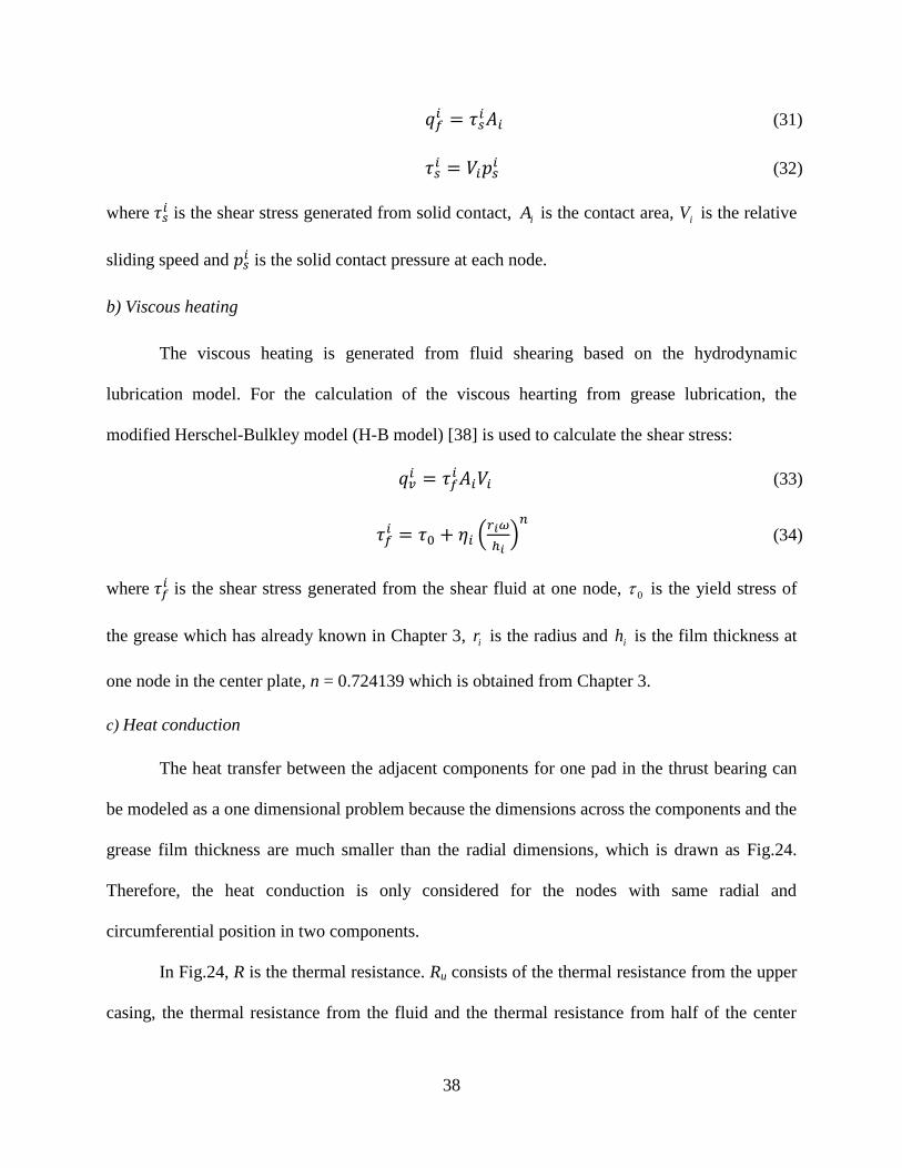
Fig.35 - Pressure distribution generated by the fluid on the center plate (fc = 33,300 m-1

, hs = 1

µm, ω = 0.14 rad/s) ....................................................................................................................... 52

Fig.36 - Total pressure distribution on the center plate (fc = 33,300 m-1

, hs = 1 µm, ω = 0.14 rad/s)

....................................................................................................................................................... 52

Fig.37 - Flow chart of the mixed lubrication calculation without thermal effects ....................... 55

Fig.38 - Film thickness distribution between one pad of the center plate and the upper case

without thermal influence (fc = 33,300 m-1

, hs = 1 µm, ω = 0.14 rad/s) ....................................... 55

x

Fig.39 - Mechanical deformation of one pad in the center plate without thermal influence (fc =

33,300 m-1

, hs = 1 µm, ω = 0.14 rad/s) ......................................................................................... 56

Fig.40 - Contact area distribution of one pad in the center plate without thermal influence (fc =

33,300 m-1

, hs = 1 µm, ω = 0.14 rad/s) ......................................................................................... 56

Fig.41- Pressure distribution from solid contact on one pad of the center plate without thermal

influence (fc = 33,300 m-1

, hs = 1 µm, ω = 0.14 rad/s).................................................................. 57

Fig.42 - Pressure distribution from fluid on one pad of the center plate without thermal influence

(fc = 33,300 m-1

, hs = 1 µm, ω = 0.14 rad/s) ................................................................................. 57

Fig.43 - Total pressure distribution on one pad of the center plate without thermal influence (fc =

33,300 m-1

, hs = 1 µm, ω = 0.14 rad/s) ......................................................................................... 58

Fig.44 - Relationship between the minimum film thickness (hmin) and the contact area ratio (A*)

for the situations with and without considering thermal influence ............................................... 59

Fig.45 - Relationship between the minimum film thickness (hmin) and the load carrying capacity

(Ltotal) for the situations with and without considering thermal influence .................................... 60

Fig.46 - Relationship between the minimum film thickness (hmin) and the frictional torque (Ttotal)

for the situations with and without considering thermal influence ............................................... 60

Fig.47 - Relationship between the minimum film thickness (hmin) and the ratio of the load

carrying capacity from fluid (Lf) and the load carrying capacity from solid contact (Ls) ............. 61

Fig.48 - Relationship between the minimum film thickness (hmin) and the ratio of the frictional

torque from fluid (Tf) and the frictional torque from solid contact (Ts) ........................................ 61

Fig.49 - Rough surface with 2048 2048 nodes from thrust bearing ........................................... 64

Fig.50 - Plot of the roughness-length method in calculating fractal dimension value for the

measured surface ........................................................................................................................... 66

Fig.51 - Film thickness between the measured surface and the upper casing (fc = 33,300 m-1

, hs =

1 µm, ω = 0.14 rad/s) .................................................................................................................... 67

Fig.52 - Mechanical deformation of the measured surface (fc = 33,300 m-1

, hs = 1 µm, ω = 0.14

rad/s) ............................................................................................................................................. 68

Fig.53 - Contact area ratio on each node of the measured surface (fc = 33,300 m-1

, hs = 1 µm, ω =

0.14 rad/s) ..................................................................................................................................... 68

Fig.54 - Solid contact pressure distribution on the measured surface (fc = 33,300 m-1

, hs = 1 µm,

ω = 0.14 rad/s) .............................................................................................................................. 69

xi

Fig.55 - Fluid pressure distribution on the measured surface (fc = 33,300 m-1

, hs = 1 µm, ω = 0.14

rad/s) ............................................................................................................................................. 69

Fig.56 - Total pressure distribution on the measured surface (fc = 33,300 m-1

, hs = 1 µm, ω = 0.14

rad/s) ............................................................................................................................................. 70

Fig.57 - Surface generated by using Eq. (52) ............................................................................... 71


surface generated by the PSD generated method .......................................................................... 72

Fig.59 - Film thickness of the PSD generated surface (fc = 33,300 m-1

, hs = 1 µm, ω = 0.14 rad/s)

....................................................................................................................................................... 73 Fig.60 - Mechanical deformation of the PSD generated surface (fc = 33,300 m

-1, hs = 1 µm, ω =

0.14 rad/s) ..................................................................................................................................... 74

Fig.61 - Contact area ratio at each node of the PSD generated surface (fc = 33,300 m-1

, hs = 1 µm,

ω = 0.14 rad/s) .............................................................................................................................. 74

Fig.62 - Solid contact pressure distribution on the PSD generated surface (fc = 33,300 m-1

, hs = 1

µm, ω = 0.14 rad/s) ....................................................................................................................... 75


, hs = 1

µm, ω = 0.14 rad/s) ....................................................................................................................... 75

Fig.64 - Total pressure distribution on the PSD generated surface (fc = 33,300 m-1

, hs = 1 µm, ω =

0.14 rad/s) ..................................................................................................................................... 76

Fig.65 - Generated process of the midpoint displacement method ............................................... 77

Fig.66 - Surface generated by midpoint displacement method..................................................... 78

Fig.67 - Plot of the roughness-length method in calculating fractal dimension value for the MDM

generated method .......................................................................................................................... 79

Fig.68 - Film thickness of the MDM generated surface (fc = 33,300 m-1

, hs = 1 µm, ω = 0.14

rad/s) ............................................................................................................................................. 80

Fig.69 - Mechanical deformation of the MDM generated surface (fc = 33,300 m-1

, hs = 1 µm, ω =

0.14 rad/s) ..................................................................................................................................... 80 Fig.70 - Contact area distribution of the MDM generated surface (fc = 33,300 m

-1, hs = 1 µm, ω =

0.14 rad/s) ..................................................................................................................................... 81

xii

Fig.71 - Solid contact pressure distribution of the MDM generated surface (fc = 33,300 m-1

, hs =

1 µm, ω = 0.14 rad/s) .................................................................................................................... 81

Fig.72 - Fluid pressure distribution of the MDM generated surface (fc = 33,300 m-1

, hs = 1 µm, ω

= 0.14 rad/s) .................................................................................................................................. 82

Fig.73 - Total pressure distribution of the MDM generated surface (fc = 33,300 m-1

, hs = 1 µm, ω

= 0.14 rad/s) .................................................................................................................................. 82

Fig.74 - Relationship between the total load carrying capacity (Ltotal) and the angular velocity (ω)

....................................................................................................................................................... 85

Fig.75 - Relationship between the load carrying capacity from the solid contact (Ls) and the

angular velocity (ω) ...................................................................................................................... 86

Fig.76 - Relationship between the ratio of the load carrying capacity from the fluid (Lf) and the

load carrying capacity from the solid contact (Ls) and the angular velocity (ω) .......................... 86

Fig.77 - Relationship between the total frictional torque (Ttotal) and the angular velocity (ω) ..... 87

Fig.78 - Relationship between the frictional torque from the solid contact (Ts) and the angular

velocity (ω) ................................................................................................................................... 87

Fig.79 - Relationship between the ratio of the frictional torque from the fluid (Tf) and the

frictional torque from the solid contact (Ts) and the angular velocity (ω) .................................... 88

Fig.80 - Relationship between the contact area ratio (A*) and the angular velocity (ω) .............. 88

Fig.81 - Relationship between the minimum film thickness (hmin) and the angular velocity (ω) . 89

Fig.82 - Relationship between the total load carrying capacity (Ltotal) and the cut-off frequency (fc)

....................................................................................................................................................... 93

Fig.83 - Relationship between the total frictional torque (Ttotal) and the cut-off frequency (fc) ... 93

Fig.84 - Relationship between the contact area ratio (A*) and the angular velocity (ω) at different

initial surface separations for the measured surface ..................................................................... 95


initial surface separations for the PSD generated surface ............................................................. 96


initial surface separations for the MDM generated surface .......................................................... 96 Fig.87 - Relationship between the load carrying capacity (Ltotal) and the angular velocity (ω) at

different initial surface separations for the measured surface ...................................................... 97

xiii

Fig.88 - Relationship between the load carrying capacity (Ltotal) and the angular velocity (ω) at

different initial surface separations for the PSD generated surface .............................................. 97


different initial surface separations for the MDM generated surface ........................................... 98

Fig.90 - Relationship between the ratio (Lf/Ls) of the load carrying capacity from fluid and the

load carrying capacity from solid contact and the angular velocity (ω) at different initial surface

separations for the measured surface ............................................................................................ 98



separations for the PSD generated surface .................................................................................... 99 Fig.92 - Relationship between the ratio (Lf/Ls) of the load carrying capacity from fluid and the


separations for the MDM generated surface ................................................................................. 99

Fig.93 - Relationship between the total frictional torque (Ttotal) and the angular velocity (ω) at

different initial surface separations for the measured surface .................................................... 100


different initial surface separations for the PSD generated surface ............................................ 100


different initial surface separations for the MDM generated surface ......................................... 101

Fig.96 - Relationship between the ratio (Tf/Ts) of the frictional torque from fluid and the

frictional torque from solid contact and the angular velocity (ω) at different initial surface

separations for the measured surface .......................................................................................... 101



separations for the PSD generated surface .................................................................................. 102



separations for the PSD generated surface .................................................................................. 102

Fig.99 - New generated surface (surface A) based on large scale roughness of the measured

surface data and small scale roughness of the PSD generated surface data ............................... 104 Fig.100 - New generated surface (surface B) based on the small scale roughness of the measured

surface data and large scale roughness of the PSD generated surface data ................................ 105

Fig.101 - Plot of the roughness-length method in calculating fractal dimension value for surface

A .................................................................................................................................................. 106

xiv


B .................................................................................................................................................. 106

Fig.103 - Changing trend between the minimum film thickness (hmin) and the total load carrying

capacity (Ltotal) ............................................................................................................................ 109

Fig.104 - Changing trend between the minimum film thickness (hmin) and the total frictional

torque (Ttotal)................................................................................................................................ 110

Fig.105 - Relationship between the cut-off frequency (fc) and the RMS roughness (Rq) ........... 112

Fig.106 - Relationship between the cut-off frequency (fc) and the Skewness (Sk) ..................... 113

Fig.107 - Relationship between the cut-off frequency (fc) and the Kurtosis (K) ........................ 113

Fig.108 - Relationship between the cut-off frequency (fc) and the fractal dimension (D) ......... 114

Fig.109 - Large scale geometry generated by Eq.(62) (b = 5, fc = 14,286 m-1

) .......................... 118

Fig.110 - Sample of generated surface (b = 5, fc = 14,286 m-1

) .................................................. 119

Fig.111 - Flow chart of calculation process with load balance................................................... 120

Fig.112 - Flow chart of optimization process ............................................................................. 121

Fig.113 - Relationship between b and load carrying capacity from fluid (Lf) ............................ 122

Fig.114 - Relationship between b and the ratio between the load carrying capacity from fluid (Lf)

and the load carrying capacity from solid contact (Ls) ............................................................... 123

Fig.115 - Relationship between b and minimum film thickness with defection (hmin) ............... 123

Fig.116 - Optimized surface shape when b = 15 (fc = 14,286 m-1

) ............................................. 124

Fig.A1 - Relationship between the load carrying capacity (Ltotal) and the cut-off frequency (fc) for

different angular velocity (ω) ..................................................................................................... 135

Fig.B1 - Relationship between the minimum film thickness (hmin) and the total frictional torque

(Ttotal) for different cut-off frequency ......................................................................................... 136

Fig.C1 - Changing trend between the cut-off frequency (fc) and the total load carrying capacity

(Ltotal) ........................................................................................................................................... 138

xv

Fig.D1 - Changing trend between the cut-off frequency (fc) and the total frictional torque

(Ttotal) …………………………………………………………………………………………...140

xvi

LIST OF TABLES

Table 1 - Three tested data of the shear rate and shear stress of the grease .................................. 20

Table 2 - Parameter values in the modified H-B model ............................................................... 21

Table 3 - Tested values of the shear rate and the viscosity ........................................................... 23

Table 4 - Basic parameters calculated for the measured rough surface ........................................ 31

Table 5 - Values of load carrying capacity and the frictional torque with considering thermal (fc =

33,300 m-1

, hs = 1 µm, ω = 0.14 rad/s) ......................................................................................... 53

Table 6 - Values of load carrying capacity and the frictional torque without considering thermal

effects (fc = 33,300 m-1

, hs = 1 µm, ω = 0.14 rad/s) ...................................................................... 58

Table 7 - Values of the load carrying capacity and the frictional torque for the measured surface

(fc = 33,300 m-1

, hs = 1 µm, ω = 0.14 rad/s) ................................................................................. 70 Table 8 - Values of the load carrying capacity and the frictional torque for the PSD generated

surface (fc = 33,300 m-1

, hs = 1 µm, ω = 0.14 rad/s) ..................................................................... 76

Table 9- Basic parameters calculated for the measured surface, the PSD generated surface and

the MDM generated surface .......................................................................................................... 79

Table 10 - Values of the load carrying capacity and the frictional torque for the PSD generated


, hs = 1 µm, ω = 0.14 rad/s) ..................................................................... 83

Table 11 - Related parameters calculated for surface A, surface B, the measured surface and the

PSD generated surface ................................................................................................................ 105

Table 12 - Some parameters calculated based on different cut-off frequencies ......................... 107

xvii

LIST OF ABBREVIATYONS

𝐴𝑛 Nominal contact area

𝐴∗ Contact area ratio

a Radius of the contact circle

D Fractal dimension

E Equivalent Young’s modulus

fc Cut-off frequency

H Hurst exponent

h Nominal film thickness

hmin Minimum film thickness

hm Separation of the mean surface height

hs Initial surface separation

K Kurtosis

Influence coefficient

k Thermal conductivity

L Load carrying capacity

l Length of measured surface

nw Total number of square windows

p Uniform pressure

p0 Maximum pressure

ijklk

xviii

Q Volumetric heat

q0 Cut-off wave vector

q Wave vector

R Thermal resistance

RA Asperity radius

Rq (σ) Root mean square roughness

r Radius of the center plate

Sk Skewness

T Frictional torque

TT Temperature

TT0 Ambient temperature

u Surface deformation

V Relative sliding speed

w Side length

zj Residuals of the asperity height

𝑧̅ Mean residual asperity height

α Thermal expansion coefficient

Pressure flow factors in r direction

Pressure flow factors in θ direction

s Shear flow factor

η Viscosity of lubrication

ηs Asperity density

σs Root mean square of the asperity height in GW model

r

xix

ν Poisson’s ratio

τ Shear stress

τ0 Yield stress of the grease

�̇� Shear rate

λ Wavelength of the surface

µ Expectation of the distribution

ω Angular velocity

θ0 Angle of one edge of the pad without grooves

θ1 Angle of the other edge of the pad without grooves

1

CHAPTER 1

INTRODUCTION AND LITERATURE REVIEW

Thrust bearings are a special type of bearings which can support an axial force (acts

parallel to the axis of rotation). It can also be called a flat faced bearing and is widely used in

many rotary industrial applications, like the steering wheel, automatic transmission and engines.

The investigation of the behavior of the bearings had received attentions for several decades, but

most of the researches are focused on the analysis of the behaviors of journal bearings [1-11],

rarely works have concerned the behavior of the flat faced thrust bearings.

The research of thrust bearings lies in many aspects, like the number of the grooves

number, the shape of the grooves and thermal effect on the thrust bearings. Brockwell, et al. [12]

changed the groove number in the thrust bearing from two to six to investigate the influence of

the groove number experimentally. He concluded that four pads seem to be the optimized

number in a thrust bearing.

In 1987, Heshmat, et al. [13] concerned with the performance of gas lubricated compliant

thrust bearing, their work offered an analytical study of the elastohydrodynamics of the thrust

bearing and the geometric parameters of the thrust bearing were also optimized to obtain the

highest load carrying capacity. Heshmat also pointed out that the load carried by the asperities

cannot be modeled by the classical Reynolds hydrodynamic analysis.

Carpino [14] investigated the flexible flat land thrust bearing at low speeds in 1990. In his

work, point loads were applied to the thrust bearing to cause the surface deflection of the thrust

2

bearing. Therefore, the converging clearances necessary for hydrodynamic lubrication can be

created by the surface deflection. His work is perhaps the same as ours, except that he treated the

fluid film between the disk and the plate as incompressible.

Most recently, the effects of groove geometry on the hydrodynamic lubrication thrust

bearings were studied by Yu and Sadeghi [15] through developing a numerical model. Their

work showed us that with proper groove geometries, the thrust bearing can support a significant

amount of load for particular operating conditions and the thrust bearing has an optimum value

of groove depth to support the maximum load carrying capacity. Yu also found that the number

of grooves can have an influence on the load support mechanism, as Brockwell [12] also

concluded, and there exists a critical characteristic number, γcr, for the groove number so that the

load capacity can be diminished.

Over the years, the thermal effect on the thrust bearing was also considered in analyzing

the behavior of the thrust bearing. Cameron and Wood [16] presented a general form of the

theory for a grooved parallel surface thrust bearing while considering the thermal deformations,

they assumed that the heat conducted away from the oil film through the metal can be neglected

and the constant temperature exists across the film.

Taniguchi and Ettles [17] did some research on the parallel surface thrust bearing as

well. In their work, a distorted film shape was displayed by using an optical interference method.

It was concluded that thrust washers with random waviness tended to perform better than lapped

bearings. It should be noted that the material of the bearing they used was aluminum to

accentuate thermal expansion, which is not the same as what we used in our work.

In addition to considering the groove geometry effect on the thrust bearing, Yu and

Sadeghi [18] discussed the thermal effects in the thrust bearing. They found that thermal effects

3

can increase the side flow rate as well as reduce the load carrying capacity and the frictional

torque. Meanwhile, thermal effects had a greater influence with the increase of the groove depth

and groove numbers. Moreover, certain operating conditions existed before thermal effects

dominated the thrust washer performance.

Meanwhile, Jackson and Green also did some research on the behavior of the thrust

bearings. In 2006, Jackson and Green [19] investigated the behavior of the thrust bearings under

the mixed lubrication and asperity contact. Thermoelastic deformations were considered later on

and the relevant work was published in [20]. Both of these works predicted the frictional torque,

bearing temperature, hydrodynamic lift and other indicators of bearing performance by coupling

sliding friction, boundary lubrication, asperity contact and full-film lubrication together, which

will also be considered in the current work.

During the analysis of the thrust bearing, rough surfaces also play an important role in the

performance of thrust bearings since the roughness can affect the wear, friction and sealing

behavior of contact surfaces. Therefore, effective characterization of surface roughness is a

significant problem.

It can be found that typically the study of thrust bearings mainly focused on the groove

effects [15], its behavior under mixed lubrication or hydrodynamic lubrication conditions [19,

21], and the thermal effects on the thrust washer [17, 18, 20]. Rarely works have combined the

mixed lubrication analysis and the surface roughness effects together to analyze the behavior of a

thrust bearing.

According to previous studies, essentially two different types of geometries are utilized in

surfaces: Euclidean geometry and fractal geometry. Euclidean geometry has long been used to

describe numerous natural phenomena. However, this kind of geometry has many limitations

4

because it can be difficult to compute the multi-scale roughness of a real world geometry. To

better characterize “rough” phenomena in both natural and artificial worlds, new approaches

needed to be introduced in addition to Euclidean geometry. Arguably, Mandelbrot was the first

person who pointed out that the fractal geometry seems much more suitable for describing the

natural world, which is inherently rough on many scales [22]. Mandelbrot also defined a fractal

as “a shape made of parts similar to the whole in some way” [23].

When using the fractal geometry to characterize rough surfaces, the most important

parameter is the fractal dimension, D. It describes the space occupancy of an object and can be

used to quantify the roughness of an object. Non-fractal Euclidian geometries have integer values

for their fractal dimensions, like a line has a fractal dimension equal to one (D=1), the fractal

dimension of a plane is two (D=2) and a space has fractal dimension equals to three (D=3).

Fractal geometry can work with objects that are non-Euclidean because they have non-integer

dimensions. The non-integer fractal dimension means an object is ‘in between’ these geometries

due to features or roughness along the border of the object. For instance, one could envision that

a line could approach the geometry of a plane as its roughness increases to become very large.

Hence, roughness can be said to cause an object to have a dimension in between these

geometries.

In this work, a thrust bearing with grease lubrication under the mixed lubrication regime

is analyzed. The first aim of this work is to build a new model with consideration of the

influence of the hydrodynamic lubrication, the solid contact, the mechanical deformation, and

thermoelastic deformation, to investigate the behavior of the thrust bearing during the rotation.

Therefore, this model can make predictions of the load carrying capacity, the frictional torque,

washer temperature distribution and some other properties of the thrust bearing. The second aim

5

is to combine the elasto-hydrodynamic lubrication and the rough surface contact effects together

to analyze the effectiveness of the fractal methods in characterizing the thrust bearing surface.

The third aim of this work is to analyze if the fractal parameter can represent a real surface

adequately.

6

CHAPTER 2

METHODOLOGY

2.1 Pressure Calculation

Fig.1- Schematic of a Stribeck curve

The Stribeck curve is basically a curve describing the relationship between the coefficient

of friction and the bearing number (defined as the relative sliding velocity, N, times the viscosity

of the lubricant, η, per unit load, P). According to the Stribeck curve (see Fig.1), a lubricated

surface contact can be categorized by three regimes: the boundary lubrication regime, the mixed

lubrication regime and the hydrodynamic lubrication regime. Despite the existence of a

7

lubricating film between two contact surfaces, some surface asperities in the thrust bearing can

still come into contact because of the surface roughness. Therefore, the contact between the

thrust bearing surfaces in our work is considered to be in the mixed lubrication regime.

Normally, the mixed lubrication contact can be divided into a hydrodynamic lubrication

part and a solid contact part. In our work, the flow-factor modified Reynolds equation [24, 25] is

used to model the hydrodynamic lubrication between the interface and the Greenwood and

Williamson (GW) model [26] is used to calculate the pressure and shear stress from the solid

contact. Fig.2 illustrates the hydrodynamic lubrication part and the solid contact part in the

mixed lubrication contact. The red area means the contact part between two surfaces.

Fig.2- Illustration of hydrodynamic lubrication and the solid contact in the mixed lubrication

contact

8

According to Patir and Cheng [24, 25], the fluid pressure pf, generated by the

hydrodynamic part can be calculated by the modified Reynolds equation in the cylindrical

coordinates, which is [27]:

𝜕

𝜕𝑟(𝜙𝑟

𝑟ℎ3

𝜂

𝜕𝑝𝑓

𝜕𝑟) +

1

𝑟

𝜕

𝜕𝜃(𝜙𝜃

ℎ3

𝜂

𝜕𝑝𝑓

𝜕𝜃) = 12 (

𝑟𝜔

2

𝜕ℎ

𝜕𝜃−

𝑟𝜔

2𝜎𝜕𝜙𝑠

𝜕𝜃) (1)

𝜙𝜃 = 𝜙𝑟 = 1 − 0.9exp(−0.56𝐻) (2)

𝜙𝑠 = {1.899𝐻0.98𝑒𝑥𝑝(−0.92𝐻 + 0.05𝐻2)𝐻 ≤ 5

1.126 exp(−0.25𝐻) 𝐻 > 5 (3)

where and are the pressure flow factors and is the shear flow factor (they are all

calculated according to [28]); H = h/σ is the ratio of the nominal film thickness h to the surface

roughness σ; η is the viscosity of the lubricant. The flow factors consider how the roughness

obstructs the flow between surfaces in close proximity. Since the roughness of the thrust bearing

surface in our work is considered to be isotropic, the equations of flow factors for isotropic

surfaces are used based on Patir and Cheng [24, 25], see Eqs. (2) and (3).

The Reynolds equation is solved by the finite difference method in our work (see Fig.3).

There three different types of finite difference method: the backward difference (Eq. (4)), the

forward difference (Eq. (5)) and the center difference (Eq. (6)). The center difference is chosen

to solve the Reynolds equation in this work.

(𝑑𝑓

𝑑𝑥)𝑛=

𝑓𝑛−𝑓𝑛−1

𝑥𝑛−𝑥𝑛−1 (4)

(𝑑𝑓

𝑑𝑥)𝑛=

𝑓𝑛+1−𝑓𝑛

𝑥𝑛+1−𝑥𝑛 (5)

(𝑑𝑓

𝑑𝑥)𝑛=

𝑓𝑛+1−𝑓𝑛−1

𝑥𝑛+1−𝑥𝑛−1 (6)

r s

9

Fig.3 - Finite difference method

Greenwood and Williamson [26] derived the statistical contact models (which can also be

called GW model) in 1966. In their model, they assumed that the contact asperities have the

same radius of curvature and the contact asperities follow a Gaussian distribution when two real

rough surfaces come into contact. Eq. (7) is the Gaussian distribution function in the GW model

and the expressions of the solid contact pressure, ps, calculated by the GW model are shown in

Eq. (8).

𝜑(𝑧) =1

√2𝜋𝜎𝑠𝑒𝑥𝑝 (−

𝑧2

2𝜎𝑠2) (7)

𝑝𝑠 =4

3𝜂𝑠𝐸√𝑅 ∫ (𝑧 − ℎ)

3

2∞

𝑑𝜑(𝑧)𝑑𝑧 (8)

10

where 𝜑(𝑧) can also be called the probability function; ηs is the asperity density; 𝐸 is the

equivalent Young’s modulus; σs is the root mean square of the asperity height; R is the radius of

curvature and Eq. (8) is solved by the Simpson quadrature in our work.

According to the discussion in Chapter 1, thermal effects cannot be neglected during the

performance analysis of the thrust bearing. The temperature rise can have an influence on many

quantities of the thrust bearing system, like the deformation of the thrust washer and the

rheological properties of the grease. Fig.4 shows the flow chart of the numerical process for the

mixed lubrication analysis with coupling the mechanical deformation, thermo-elastic

deformation, hydrodynamic lubrication and solid contact together. The left half of the flow chart

shows the calculation process of the hydrodynamic half by using Reynolds equation and the right

part of it shows the calculation process of the solid contact part. The film thickness between the

two surfaces is updated every iteration. After the pressure and shear stress of the hydrodynamic

lubrication part and the solid contact part are obtained from the calculation above (the

convergence criteria for the pressure is 𝑒𝑟𝑟𝑜𝑟 ≤ 1 × 10−4 ), the frictional torque and load

carrying capacity of the thrust bearing can be calculated.

11

Fig.4 - Flow chart of the mixed lubrication analysis for the thrust bearing system

12

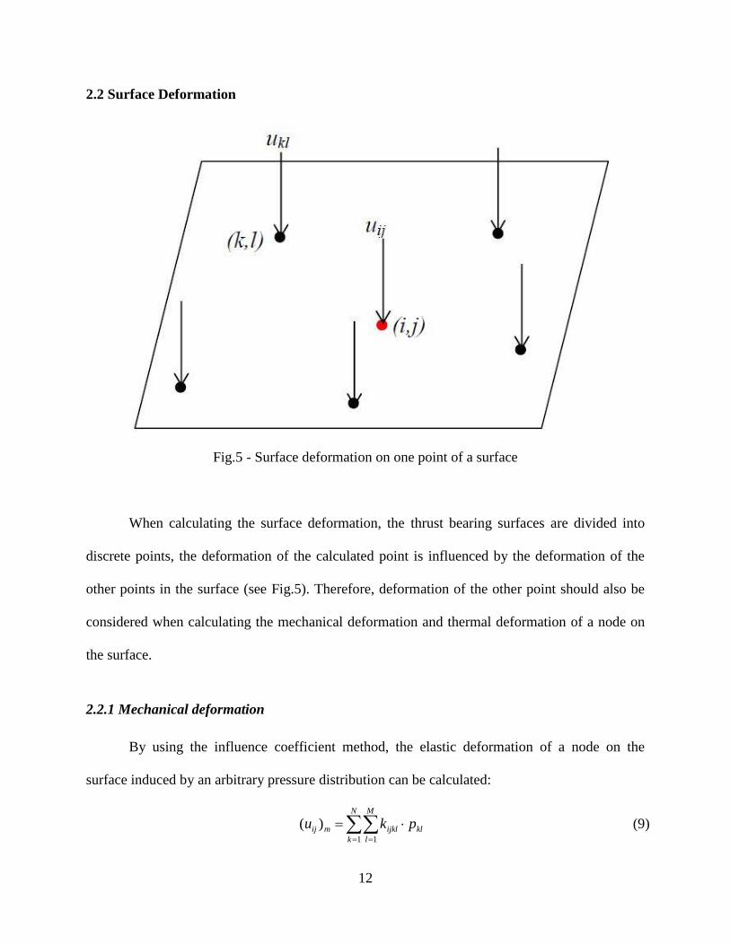
2.2 Surface Deformation

Fig.5 - Surface deformation on one point of a surface

When calculating the surface deformation, the thrust bearing surfaces are divided into

discrete points, the deformation of the calculated point is influenced by the deformation of the

other points in the surface (see Fig.5). Therefore, deformation of the other point should also be

considered when calculating the mechanical deformation and thermal deformation of a node on

the surface.

2.2.1 Mechanical deformation

By using the influence coefficient method, the elastic deformation of a node on the

surface induced by an arbitrary pressure distribution can be calculated:

kl

N

k

M

l

ijklmij pku 1 1

)( (9)

13

where miju )( is the mechanical deformation of the calculated point, ijklk is the influence

coefficient, p is the uniform pressure applied on the discrete points of the surface.

According to Love [29], the influence coefficient at a rectangular area (2a×2b) around a

node can be calculated by the equation:

2/122

2/122

2/122

2/1222

)()()(

)()()(ln)(

)()()(

)()()(ln

1

axbyax

axbyaxby

axbyby

axbybyax

E

vk

2/122

2/122

2/122

2/122

)()()(

)()()(ln)(

)()()(

)()()(ln)(

axbyax

axbyaxby

axbyby

axbybyax (10)

where ν is Poisson’s ratio.

A verification of the influence function has also been conducted by comparing to a

known solution. Suppose the contact between two elastic solid surfaces is Hertz contact (see

Fig.6), the values of the related parameters are also shown in Fig.6 (Hertz contact is spherical

contact, but it is solved in this work as a parabolic peak). The reference deformation can be

calculated according to Johnson [30]:

𝑢𝑟𝑒𝑓

{

=

1−𝜐2

𝐸

𝜋𝑝0

4𝑎(2𝑎2 − 𝑟2),𝑟 ≤ 𝑎

=1−𝜐2

𝐸

𝑝0

2𝑎{(2𝑎2 − 𝑟2)𝑠𝑖𝑛−1(𝑎 𝑟⁄ ) + 𝑟

2(𝑎 𝑟⁄ ) (1 −𝑎2

𝑟2⁄ )

12⁄

} ,𝑟 > 𝑎 (11)

where r is the radius where the contact point is located; a is the radius of the contact circle, p0 is

the maximum pressure. a and p0 can also be calculated according to Johnson [30]:

𝑎 = (3𝑃𝑅

4𝐸)13⁄

(12)

𝑝0 =3𝑃

2𝜋𝑎2 (13)

where the values of P and R can be found in Fig.6.

14

Fig.6 - Schematic illustration of Hertz contact

Fig.7 shows the plots of the deflection calculated by the influence function and the Hertz

contact theory. It can be found that the deflection calculated by the influence function is

matching satisfactorily with the deflection calculated by the Hertz contact theory, which means

that the influence function algorithm is correct and can be used in calculating the deflection of

the thrust bearing surface.

15

Fig.7 - Comparison of deflection calculated by the influence function and Hertz contact theory

2.2.2 Thermal deformation

The discretized points on the thrust bearing surface can be approximately regarded as a

circular region at uniform temperature relative to an ambient temperature, TT0, hence the

thermos-elastic deformation can be calculated according to Barber [31]:

(𝑢𝑖𝑗)𝑡 = {−2

𝜋𝑐𝑘𝑎 ((𝑇𝑇𝑖𝑗)𝑐 − 𝑇𝑇0) [𝑙𝑛 (

𝑟0

𝑎) − 𝑙𝑛 {1 + (1 −

𝑟2

𝑎2)12⁄

} + (1 −𝑟2

𝑎2)12⁄

] , 𝑟 ≤ 𝑎

−2

𝜋𝑐𝑘𝑎 ((𝑇𝑇𝑖𝑗)𝑐 − 𝑇𝑇0) 𝑙𝑛 (

𝑟0

𝑟) ,𝑟 > 𝑎

(14)

where tiju )( is the thermal deformation of the calculated point; r is the distance between the

calculated point and the other point; 0r is the position on the surface where tiju )( is zero (r0 is set

to be three times of the pad diameter in the analysis); c is the constant given by k/1 , α is

16

the thermal expansion coefficient, k is the thermal conductivity which can be determined

according to the material used in the thrust bearing;(𝑇𝑇𝑖𝑗)𝑐 is the uniform temperature of a

circular region of the calculated point; 𝑇𝑇0 is the ambient temperature, a is the radius of the

circle around the calculated point.

2.3 Fractal Dimension Calculation

As we discussed in the references [32, 33], the roughness-length method appears to be the

most effective method in calculating the fractal dimension value, so the 3D roughness-length

method [34] is used to calculate the fractal dimension of the measured thrust bearing surface in

this work.

For the 3D rough surfaces, the power law relationship between the standard deviation of

the residual surface height, S(w), and the sampling length window size, w, can be calculated by

the equation below [34]:

𝑆(𝑤) = 𝐴𝑤𝐻 (15)

where H is the Hurst exponent and A is a constant. By dividing the rough surface into a grid of

squares with the window length, w, S(w) (can also be regarded as the root-mean-square

roughness of the divided squares) can be calculated according to the following equation [34]:

w

i

n

i wj

j

iw

zzmn

wRMSwS1

2)(2

11)()( (16)

where nw is the total number of square windows with the side length, w; mi is the total number of

points in the square window, wi; zj is the residuals of the asperity height on the trend, and z is

the mean residual asperity height in each square window. For surfaces, the Hurst exponent, H, is

17

related to the fractal dimension, D, with the equation D = 3-H. H can be obtained from the slope

of the log-log plot of S(w) and w.

18

CHAPTER 3

LUBRICANT VISCOSITY

3.1 Lubricant Used

As we mentioned previously, the lubricant we used between two thrust bearing surfaces

is grease. Grease is regarded as a semisolid lubricant (it can also be called a non-Newtonian

fluid), it is made up of a base oil, additives and the thickener. Petroleum or synthetic oil is

typically used as the base oil, additives are used to modify the base oil properties and thickener is

used to control the consistency of the base oil. According to the application, the grease we used

in our work consists of G-501 (thickener) with KF-96-10 silicone oil (base oil).

Viscosity is a very important parameter used to measure the resistance of deformation for

a lubricant when a shear stress or a tensile stress applied on it. Viscosity can effect heat

generation in bearings related to a lubricant internal friction, it can also govern the sealing effect

of the lubricant. The value of the viscosity can be influenced by the temperature change and the

magnitude of the applied pressure. The grease lubricant is not the same as the frequently-used oil

lubricant, it has a high initial viscosity and its viscosity is not only related to the temperature and

the pressure but also related to the shear rate. Therefore, it is very hard to find the exact viscosity

value of the grease from the handbook.

19

3.2 Herschel-Bulkley (H-B) Model

H-B model is a generalized model for a non-Newtonian fluid (shearing-thinning or shear-

thickening), which combines the shear rate and the shear stress experienced by the fluid in a

complicated way. By combining the viscosity of the grease and the generalized H-B model, a

modified H-B model is used in this work:

𝜏 = 𝜏0 + 𝜂�̇�𝑛 (17)

where τ is the shear stress, τ0 is the yield shear stress of the grease, �̇� is the shear rate. n is the

flow index. η is the viscosity of the grease (will be discussed in Section 3.4). The fluid is shear-

thickening for n >1, the fluid is shear-thinning for n <1. Both of k and n can be calculated

according to the behavior of the grease.

Fig.8 - Physica MCR 301

20

Table 1 - Three tested data of the shear rate and shear stress of the grease

Shear rate, �̇� (s-1

) Shear stress (Pa)

First test Second test Third test

0.01 420.5340722 415.7246849 449

0.0158 423.6747764 415.8922065 454

0.0251 427.9071721 416.1608187 456

0.0398 433.5267798 416.5853994 466

0.0631 441.0115203 417.2583741 471

0.1 450.9730735 418.3241581 480

0.158 464.1409624 419.9993742 493

0.251 481.8859364 422.6854966 511

0.398 505.4470116 426.9313029 532

0.631 536.8279452 433.6610503 559

1 578.5932991 444.3188906 592

1.58 633.8017117 461.0710516 639

2.51 708.2002624 487.9322751 702

3.98 806.9837175 530.3903382 789

6.31 938.5531399 597.6878123 910

10 1113.660852 704.2662155 1080

15.8 1345.130669 871.7878248 1310

25.1 1657.05811 1140.400061 1630

39.8 2071.223039 1564.980691 2090

63.1 2622.848211 2237.955432 2740

100 3542.848211 3303.739464 3660

21

Fig.9 - Relationship between the shear stress and the shear rate of the grease

Table 2 - Parameter values in the modified H-B model

First test Second test Third test Average

Yield stress, τ0 (Pa) 525 523 565 537.67

n 0.734188 0.708968 0.729417 0.724191

A Physica MCR 301 rheometer is used (see Fig.8) to test the grease properties and the

grease is tested three times to make the measurement more accurate. Table 1 shows the three

tested data of the shear rate and shear stress. Fig.9 shows the relationship between the shear

stress and the shear rate of the grease based on the data in Table 1.

22

The intersection point of the fitted line with the y-axis is the value of the yield stress, τ0,

in Eq. (17). Table 2 shows the tested parameter values in the modified H-B model. By averaging

the values in Table 2, the yield stress of the grease, τ0, and the flow index, n, value can be

obtained. Eq. (17) is then can be used to calculate the shear stress in this work.

3.3 Lubricant Viscosity Test

By changing the shear rate value in the Physica MCR 301 rheometer, the viscosity values

of the grease will also be changed. The related viscosity values obtained from the tested machine

are listed in Table 3. Fig.10 shows the plot of the tested results for the relationship between the

averaged viscosity and the shear rate of the grease (these two values are plotted on a log-log

scale) according to Table 3. It can be found from the plot that the viscosity decreases with the

increase of the shear rate and the trend line seems to become flat when the shear rate becomes

infinity.

23

Table 3 - Tested values of the shear rate and the viscosity

Shear rate, �̇� (sec-1

) Viscosity, 𝜇𝑠 (Pa s)

First test Second test Third test Average value

0.01 49,150 41,100 44900 45,050

0.0158 32,900 30,600 31450 31,650

0.0251 20,850 19,900 20,000 20,250

0.0398 13,050 12,400 12,350 12,600

0.0631 8,225 7,940 7895 8,020

0.1 5,140 5,120 4,870 5,073

0.158 3,290 3,315 3,155 3,275

0.251 2,130 2,155 2,060 2,128

0.398 1,390 1,405 1,355 1,392

0.631 912 932 896 919

1 610 619 600 613

1.58 414 418 408 415

2.51 286 288 283 286

3.98 202 202 200 202

6.31 146 145 145 145

10 108 108 109 108

15.8 82.7 82 83 82

25.1 65.2 64 65 65

39.8 52.6 52 53 52

63.1 43.3 43 44 43

100 36.4 36 37 36

24

Fig.10 - Relationship between the averaged viscosity and the shear rate of the grease

3.4 Lubricant Viscosity Calculation

Fig.11 shows the fitted line of the log of the viscosity value and the log of the shear rate

value in Fig.10 and the fitted equation can be obtained:

𝜂𝑠𝑟 = exp(−0.00026064 × (𝑙𝑛�̇�)4 + 0.003912 × (𝑙𝑛�̇�)3

+0.041273 × (𝑙𝑛�̇�)2 − 0.85966 × (𝑙𝑛�̇�) + 6.4078) (18)

The value of shear rate �̇� can be calculated from the equation below:

�̇� =𝑟∙𝜔

ℎ (19)

where r is the radius of the center plate in the thrust bearing (which will be shown later), ω is the

angular velocity (the velocity of the thrust bearing rotated around the intermediate shaft) of the

25

thrust bearing system, h is the film thickness between the upper case and center plate (see

Chapter 4).

Fig.11 - Fitted line of the tested data in Fig.10

According to Hamrock [35], the relationship between the temperature and the viscosity of

the grease can be written as:

𝜂 = 𝜂𝑐10𝐺0(1+

𝑇𝑇𝑖135⁄ )

−𝑠0

(20)

where G0 is the dimensionless constant indicative of the viscosity grade of the liquid, s0 is the

dimensionless constant that establishes the slope of viscosity-temperature relationship. TTi is the

temperature at one node which can be calculated by the energy equation (will be discussed later),

the unit of TTi is oC; 𝜂𝑐 in Eq. (20) can be calculated by the equation:

26

𝜂𝑐 =𝜂𝑠𝑟

𝜂∞ (21)

where 𝜂∞ = 6.31e-05 Ns/m2, it is an extrapolating analytical value of viscosity when TTi tends to

be infinite and it is approximately common to all oils according to Roelands [36].

G0 and s0 in Eq. (20) can be calculated by setting 𝜂𝑐 in Eq. (20) equals to 𝜂∞:

𝜂𝑖 = 𝜂∞10𝐺0(1+

𝑇𝑇𝑖135⁄ )

−𝑠0

(22)

Since it is very hard to find the viscosity values of the grease at different temperature and

the properties of any grease are determined by the properties of the base oil, the properties of the

base oil (which is KF-96-10 silicone oil in our research) are used instead to evaluate G0 and s0

values.

According to the performance test results of KF-96-10 silicone oil in the website

(https://www.shinetsusilicone-global.com/catalog/pdf/kf96_e.pdf), when the temperature is 25oC,

the viscosity of the KF-96-10 silicone oil is 9.7 Ns/m2; when the temperature rises to 50

oC, its

viscosity decreases to 6.79 Ns/m

2. By putting these values into Eq. (20), values of G0 and s0 can

be obtained (G0 = 5.347, s0 = 0.209)

Therefore, according to the calculation above, the grease viscosity we used in our

research is:

𝜂 =exp(

−0.00026064×(𝑙𝑛�̇�)4+0.003912×(𝑙𝑛�̇�)3

+0.041273×(𝑙𝑛�̇�)2−0.85966×(𝑙𝑛�̇�)+6.4078)

6.31e−05∙ 105.347(1+

𝑇𝑇𝑖135

)−0.209

(23)

https://www.shinetsusilicone-global.com/catalog/pdf/kf96_e.pdf

27

CHAPTER 4

Numerical Methodology

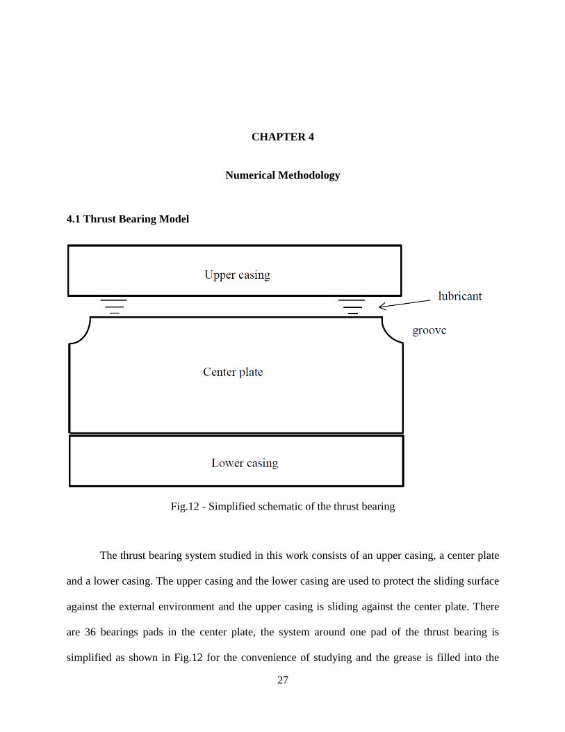
4.1 Thrust Bearing Model

Fig.12 - Simplified schematic of the thrust bearing

The thrust bearing system studied in this work consists of an upper casing, a center plate

and a lower casing. The upper casing and the lower casing are used to protect the sliding surface

against the external environment and the upper casing is sliding against the center plate. There

are 36 bearings pads in the center plate, the system around one pad of the thrust bearing is

simplified as shown in Fig.12 for the convenience of studying and the grease is filled into the

28

space between the upper case and the center plate. Fig.13 shows the coordinate setup in our

thrust bearing system, the upper case is set at the location of z = 0 so that it is easy to calculate

the shear stress (which will be shown later) .

Fig.13 - Coordinate setup in the thrust bearing system

In the work, the thrust bearing surface is scanned with a Bruker NPFLEX system and part

of it is shown in Fig.14 (the coordinate values are normalized by the outer radius value of the

thrust bearing (ro)). Because of the axisymmetric property of the thrust bearing system in our

research, the load carrying capacity and the frictional torque for one pad of the center plate is

studied and then these two values of the total bearing performance is 36 times of the values of

the load carrying capacity and the frictional torque for one pad.

29

Fig.14 - Thrust bearing surface

Fig.15 - One pad surface with radial grooves

30

One pad with two radial grooves is chosen which is shown in Fig.15 (the coordinate

values are normalized by the outer radius value of the thrust bearing (ro)). It can be found that

there are lots of high peaks near the edges, which are from the experimental noise. These peaks

are removed by replacing them with the average heights of the surrounding nodes for the better

calculation as shown in Fig.16 (the coordinate values are normalized by the outer radius value of

the thrust bearing (ro)).

As we mentioned in Chapter 2, the thrust bearing system of the application is under the

mixed lubrication regime and most of the pressure is from the solid contact part. Therefore, one

single pad surface without grooves is chosen from the refined pad surface shown in Fig.17 (the

coordinate values are normalized by the outer radius value of the thrust bearing (ro)) and the

surface data is collected.

Fig.16 - One pad surface with radial grooves after refining

31

Fig.17 - One pad surface without grooves

Table 4 - Basic parameters calculated for the measured rough surface

Parameters Values

Root mean square (Rq) 1.0200×10-5

m

Kurtosis (K) 0.0057

Skewness (Sk) -1.7321

Asperity radius (RA) 1.0241×10-5

m

Asperity density (ηs) 3.2156×1010

m-2

The collected data is leveled before being used to calculate the related surface parameters,

so that the average slope of the surface is zero. Table 4 shows some basic parameters calculated

for the pad surface.

32

Fig.18 - Simplified sketch of one pad and its coordinate in cylindrical coordinate

The surface data is measured in the Cartesian coordinates, while the Reynolds equation is

in the cylindrical coordinates (see Eq. (1) and Fig.18 shows a simplified sketch of one pad using

cylindrical coordinates). Therefore, a coordinate transformation needs to be performed on the

collected data so that the data can be used in the Reynolds equation. The in-plane coordinates

transformation are shown in Eq. (24) and Eq. (25).

𝑥 − 𝑥0 = 𝑟𝑐𝑜𝑠(𝜃) (24)

𝑦 − 𝑦0 = 𝑟𝑠𝑖𝑛(𝜃) (25)

where x0 and y0 is the origin of the center of the thrust bearing in the Cartesian coordinate.

In the z direction, four closest-neighborhood points are found in the Cartesian coordinate

and the bilinear interpolation function (Eq. (26)) is performed to map back the collected data

33

onto the cylindrical coordinate system from Cartesian coordinates. Fig.19 shows the details of

the coordinate transformation. The number of mapped nodes in the cylindrical coordinate is

60×120 (there are 60 points in the r direction and 120 points in the θ direction).

(𝑥, 𝑦) =1

(𝑥2−𝑥1)(𝑦2−𝑦1)(𝑓(𝑄11)(𝑥2 − 𝑥)(𝑦2 − 𝑦) + 𝑓(𝑄21)(𝑥 − 𝑥1)(𝑦2 − 𝑦)

+𝑓(𝑄12)(𝑥2 − 𝑥)(𝑦 − 𝑦21) + 𝑓(𝑄22)(𝑥 − 𝑥1)(𝑦 − 𝑦1)) (26)

where x1, x2, y1 and y2 are the coordinate values of points in the Cartesian coordinate, Q11 = (x1,

y1), Q12 = (x1, y2), Q21 = (x2, y1) and Q22 = (x2, y2); f(Q11), f(Q12) f(Q21) and f(Q22) are the point

heights in Cartesian coordinates and f (x, y) is the point height in cylindrical coordinates.

Fig.19 - Coordinate transformation from Cartesian coordinate to cylindrical coordinate

34

Fig.20 - Process of surface deconstruction

After the thrust washer surface is collected, the surface is deconstructed into small scale

roughness and large scale roughness via a filtering algorithm according to a cut-off frequency.

The parameters of the rough surface contact and the flow factors are calculated according to the

small scale roughness, and the Reynolds equation and the surface deflection are solved based on

the large scale geometry. Fig.20 shows the process of surface deconstruction and Fig.21 explains

this process by figures (the coordinate values are normalized by the outer radius value of the

thrust bearing (ro)). By combining the small scale roughness part via rough surface contact and

flow factors and the large scale geometry part together from Reynolds Equation (Eq. (1)) and

macro-scale surface deformation, our bearing model is formed.

35

Fig.21 - Process of surface deconstruction illustrated by figures

4.2 Heat Balance

In our analysis, the two-dimensional steady-state heat transfer equation from Özisik [37]

under the cylindrical coordinates is used:

𝜕2𝑇𝑇

𝜕𝑟2+

1

𝑟

𝜕𝑇𝑇

𝜕𝑟+

1

𝑟2

𝜕2𝑇𝑇

𝜕𝜃2+

1

𝑘𝑄(𝑟, 𝜃) = 0 (27)

where TT is the temperature distributed around each point, Q(r,θ) is the volumetric heat in the

thrust bearing, it has three possible sources: a) the fractional heating from solid contact; b) the

Original surface

Small scale roughness Large scale roughness

36

viscous heating from fluid shearing; c) the heat conducted to or from adjacent points on the

thrust washer components. These sources will be described in detail later.

4.2.1 Code verification

Fig.22 - Generic geometry for energy equation code verification

To verify our code for the energy equation used to calculate the temperature distribution

around each point, a generic geometry under the axisymmetric condition without heat conduction

is considered (see Fig.22). Then the energy equation can be written as Eq. (28) in this situation.

𝜕2𝑇𝑇

𝜕𝑟2+

1

𝑟

𝜕𝑇𝑇

𝜕𝑟= 0 (28)

The analytical solution of Eq. (28) for the generic geometry is shown as Eq. (29) and the

discretized numerical solution for Eq. (28) can also be obtained (see Eq. (30)).

37

𝑇𝑇 =5

𝑙𝑛3𝑙𝑛(𝑟) + 25 (29)

(1

∆𝑟2−

1

2𝑟∆𝑟) 𝑇𝑇𝑖−1.𝑗 −

2

∆𝑟2𝑇𝑇𝑖,𝑗 + (

1

∆𝑟2+

1

2𝑟∆𝑟) 𝑇𝑇𝑖+1,𝑗 = 0 (30)

Fig.23 - Generic geometry for energy equation code verification

Fig.23 shows the results of temperature change calculated from the numerical solution

and the analytical solution. The changing trends from these two solutions are effectively the

same which indicates that the code for solving the energy equation is valid.

4.2.2 Volumetric heat calculation

a) Frictional heating

After the solid contact pressure is obtained based on the solid contact model (Eq. (8)), the

equation of frictional heating at each node can be written as:

38

𝑞𝑓𝑖 = 𝜏𝑠

𝑖𝐴𝑖 (31)

𝜏𝑠𝑖 = 𝑉𝑖𝑝𝑠

𝑖 (32)

where 𝜏𝑠𝑖 is the shear stress generated from solid contact, iA is the contact area, iV is the relative

sliding speed and 𝑝𝑠𝑖 is the solid contact pressure at each node.

b) Viscous heating

The viscous heating is generated from fluid shearing based on the hydrodynamic

lubrication model. For the calculation of the viscous hearting from grease lubrication, the

modified Herschel-Bulkley model (H-B model) [38] is used to calculate the shear stress:

𝑞𝑣𝑖 = 𝜏𝑓

𝑖𝐴𝑖𝑉𝑖 (33)

𝜏𝑓𝑖 = 𝜏0 + 𝜂𝑖 (

𝑟𝑖𝜔

ℎ𝑖)𝑛

(34)

where 𝜏𝑓𝑖 is the shear stress generated from the shear fluid at one node, 0 is the yield stress of

the grease which has already known in Chapter 3, ir is the radius and ih is the film thickness at

one node in the center plate, n = 0.724139 which is obtained from Chapter 3.

c) Heat conduction

The heat transfer between the adjacent components for one pad in the thrust bearing can

be modeled as a one dimensional problem because the dimensions across the components and the

grease film thickness are much smaller than the radial dimensions, which is drawn as Fig.24.

Therefore, the heat conduction is only considered for the nodes with same radial and

circumferential position in two components.

In Fig.24, R is the thermal resistance. Ru consists of the thermal resistance from the upper

casing, the thermal resistance from the fluid and the thermal resistance from half of the center

39

plate. Rl includes the thermal resistance from half of the center plate and the thermal resistance

from lower casing. TT0 is the ambient temperature which is set to be 25°C and TTc is the

temperature of center plate. In this work, Heat convection is not considered because of its

expected small value compared with the heat conduction. In addition, the temperature of one pad

is considered as periodical in the circumference direction and the temperature in the inner and

outer radii is also set to equal to TT0 (25°C) (see Fig.25).

Fig.24 - Schematic of heat transfer between components (not drawing for scale)

40

Fig.25 - Periodical temperature in circumference direction

The heat conducted between components can be calculated by using the thermal

resistance according to [20, 39]:

𝑅𝑢 = 𝑅𝑓𝑙𝑢𝑖𝑑 + 𝑅𝑢𝑝𝑝𝑒𝑟 +𝑅𝑐𝑒𝑛𝑡𝑒𝑟

2=

ℎ𝑚

𝑘𝑓𝑙𝑢𝑖𝑑+

𝑡𝑢𝑝𝑝𝑒𝑟

𝑘𝑢𝑝𝑝𝑒𝑟+

𝑡𝑐𝑒𝑛𝑡𝑒𝑟

2𝑘𝑐𝑒𝑛𝑡𝑒𝑟 (35)

𝑅𝑙 = 𝑅𝑙𝑜𝑤𝑒𝑟 +𝑅𝑐𝑒𝑛𝑡𝑒𝑟

2=

𝑡𝑙𝑜𝑤𝑒𝑟

𝑘𝑙𝑜𝑤𝑒𝑟+

𝑡𝑤𝑎𝑠ℎ𝑒𝑟

2𝑘𝑤𝑎𝑠ℎ𝑒𝑟 (36)

where t is the thickness of each component; kfluid is the thermal conductivity of the grease that

can be determined according to the property of base oil (KF-96-10 silicone oil) in the grease;

kupper, kcenter and klower are the thermal conductivity of the upper casing, center plate and lower

casing, these three values can all be determined for the particular materials of the upper casing,

the center plate and the lower casing; hm is the separation of the mean surface height between

41

upper casing and the center plate. Then the conducted heating along z direction for a node i in

component a to the same location in the adjacent component b is:

𝑞𝑐𝑖 =

𝑇𝑇𝑎−𝑇𝑇𝑏

𝑅𝑎→𝑏 (37)

After all the heating parts are calculated, the volumetric heat around one node can be

obtained by:

𝑄𝑖(𝑟, 𝜃) =(𝑞𝑓𝑖+𝑞𝑣

𝑖 )

𝑡𝑖𝐴𝑖+

𝑞𝑐𝑖

𝑡𝑖 (38)

where ti is the thickness of the component at node i.

Since the heat convection is not considered, the temperature change in the boundary

nodes can be ignored and only the internal nodes temperature change is calculated. By taking Eq.

(38) into Eq. (27) and using the finite difference method, the discretized temperature (TTi,j)

expression for internal nodes solved by the energy equation is shown below:

𝑇𝑇𝑖,𝑗 =[(

1

∆𝑟2+

1

2𝑟∆𝑟)𝑇𝑇𝑖,𝑗+(

1

∆𝑟2−

1

2𝑟∆𝑟)𝑇𝑇𝑖−1,𝑗+

1

𝑟2∆𝜃2𝑇𝑇𝑖,𝑗+1+

1

𝑟2∆𝜃2𝑇𝑇𝑖,𝑗−1+

1

𝑘𝑄𝑖,𝑗]

(2

∆𝑟2+

2

𝑟2∆𝜃2)

(39)

The Gauss-Seidel method is used to solve for the temperature between two nodes in the

adjacent components according to Eq. (39). Then the calculated temperature value can be put

back in Eq. (14) to compute the thermal deformation.

4.3 Contact Area Ratio

Contact area ratio is a measure of how much actual area come into contact during the

rotation of the thrust bearing system. When two surfaces come into contact, only asperities on

the surfaces can come into contact since the existence of the roughness on the surface. Therefore,

surface roughness can decrease the real area of contact. The contact area ratio around one

measured point can be calculated according to Greenwood and Williamson [26]:

42

𝐴𝑖𝑗∗ = 𝜂𝑠𝜋𝑅 ∫ (𝑧 − ℎ)𝜙(𝑧)𝑑𝑧

∞

𝑑 (40)

Fig.26 - Simplified drawing of the center plate

The center plate can be regarded as an annulus (see Fig.26), and the area of an annulus

can be calculated by using Eq. (41). Since there are 36 pads in one center plate, then the nominal

contact area for one pad is given by Eq. (42).

𝐴𝑎 = 𝜋(𝑟𝑂2 − 𝑟𝐼

2) (41)

𝐴𝑛 =𝜋(𝑟𝑂

2−𝑟𝐼2)

36 (42)

Fig.27 shows the nominal contact area around one point and there are 120 points in the θ

direction as we illustrated previously, so that these 120 points can be regarded as 119 nominal

43

contact areas as shown in Fig.27 in the θ direction. Therefore, the nominal contact area around

one point can be calculated:

𝐴𝑖𝑗 =𝜋(𝑟𝑂

2−𝑟𝐼2)

36×119 (43)

Fig.27 - Nominal contact area around one point

Eq. (44) describes the real contact area around one point. By double summing the real

contact area around one point and dividing the nominal contact area of one pad, the contact area

ratio can be calculated (shown in Eq. (45)).

(𝐴𝑟)𝑖𝑗 = 𝐴𝑖𝑗∗ ∙ 𝐴𝑖𝑗 (44)

𝐴∗ =∑∑(𝐴𝑟)𝑖𝑗

𝐴𝑛 (45)

The real contact area will later be considered when analyzing the bearing bearings.

44

4.4 Load Carrying Capacity and Frictional Torque

According to Fig.4, after the solid contact pressure and the fluid pressure are calculated

based on Eq. (1) and Eq. (3), the values of the load carrying capacity and the frictional torque

from the solid contact and the fluid can be computed. By adding the load carrying capacity and

the frictional torque values from the solid contact and the fluid, the total load carrying capacity

and the frictional torque for the thrust bearing system can be obtained.

It should be noted that during the calculation of the pressure from the hydrodynamic part,

the periodic boundary conditions in θ direction are considered:

𝑝(𝑟, 𝜃0) = 𝑝(𝑟, 𝜃1) (46)

𝜕𝑝

𝜕𝑟(𝑟, 𝜃0) =

𝜕𝑝

𝜕𝑟(𝑟, 𝜃1) (47)

where θ0 and θ1 are angles of the edges of the pad without grooves.

4.4.1 Load carrying capacity and frictional torque from solid contact

According to Eq. (3), the solid contact pressure can be calculated, and the expression of

load carrying capacity acting on the periodic center plate generated by the solid contact part is:

𝐿𝑠 = ∫ ∫ 𝑝𝑠(𝑟, 𝜃)𝑟𝑑𝑟𝑑𝜃𝑟𝑜

𝑟𝑖

𝜃1

𝜃0 (48)

Fig.28 shows the direction of shear stress components, τzr and τzθ, acting on one pad

generated by the contact asperities. Since τzr has no contribution to the solid contact frictional

torque, Ts, during the rotation, τzθ (referred as τs) is the only shear stress considered when

calculating the frictional torque from solid contact. The expression of τs has been shown in Eq.

(32), and the frictional torque generated by the solid contact, Ts, can be evaluated by the double

integral of τs:

45

𝑇𝑠 = ∫ ∫ 𝜏𝑠(𝑟, 𝜃)𝑟2𝑑𝑟𝑑𝜃

𝑟𝑜

𝑟𝑖

𝜃1

𝜃0 (49)

Fig.28 - Shear stress components on the upper casing

4.4.2 Load carrying capacity and frictional torque from fluid

The fluid pressure can be calculated based on Eq. (1). The expression of load carrying

capacity acting on the periodic pad generated by the fluid follows the same form as the

expression of load carrying capacity generated by the solid contact part:

𝐿𝑓 = ∫ ∫ 𝑝𝑓(𝑟, 𝜃)𝑟𝑑𝑟𝑑𝜃𝑟𝑜

𝑟𝑖

𝜃1

𝜃0 (50)

Since the lubricant we used is grease, the shear stress from fluid, τf, can be calculated by

the Herschel-Bulkley model (H-B model) [38] (see Eq. (34)). By double integrating τf, the

frictional torque generated from the fluid, Tf, can be obtained:

𝑇𝑓 = ∫ ∫ 𝜏𝑓(𝑟, 𝜃)𝑟2𝑑𝑟𝑑𝜃

𝑟𝑜

𝑟𝑖

𝜃1

𝜃0 (51)

46

4.4.3 Total Load carrying capacity and frictional torque

The total pressure acting on the pad can be calculated by adding the pressure from the

solid contact,𝑝𝑠, and the fluid, 𝑝𝑓, together and the total load carrying capacity can be calculated

according to Eq. (53):

𝑝𝑡𝑜𝑡𝑎𝑙 = 𝑝𝑠 + 𝑝𝑓 (52)

𝐿𝑡𝑜𝑡𝑎𝑙 = ∫ ∫ 𝑝𝑡𝑜𝑡𝑎𝑙(𝑟, 𝜃)𝑟𝑑𝑟𝑑𝜃𝑟𝑜

𝑟𝑖

𝜃1

𝜃0 (53)

After the shear stresses from the solid contact, τs, and the fluid, τf, are obtained, the total

shear stress acting on the pad can be computed by adding these two shear stresses together:

𝜏𝑡𝑜𝑡𝑎𝑙 = 𝜏𝑠 + 𝜏𝑓 (54)

Then the total frictional torque can be evaluated by double integrating the total shear

stress, τtotal:

𝑇𝑡𝑜𝑡𝑎𝑙 = ∫ ∫ 𝜏𝑡𝑜𝑡𝑎𝑙(𝑟, 𝜃)𝑟2𝑑𝑟𝑑𝜃

𝑟𝑜

𝑟𝑖

𝜃1

𝜃0 (55)

47

Chapter 5

Results and Analysis for New Bearing Model

5.1 Results with Consideration of Thermal Effects

This chapter shows the results of the indicators of thrust bearing system in this work. The

results are based on a coupled model of the mechanical deformation, thermo-elastic deformation,

hydrodynamic lubrication, solid contact and grease influence together. It should be noted here

that since the surface is deconstructed according to the cut-off frequency, the results shown

below are for a specific case when the cut-off frequency, fc, is 33,300 m-1

, and the initial surface

separation, hs is 1 µm. The angular velocity used for the specific case based on an application of

this bearing is 0.14 rad/s based on an application of this bearing.

Fig.29 shows the film thickness distribution between the center plate and the upper casing,

and the film thickness is very small at the boundary of the center plate. Fig.30 shows the

temperature distribution of the center plate according to Eq. (39). The temperature is much

higher at the boundary of the center plate than at the inside of the center plate.

It is obvious that a thinner local film thickness generates much higher temperature by

comparing Figs. 29 and 30. Because there will be more solid contact at local small film thickness

and solid contact can generate more friction and heat than fluid shearing, most of the temperature

is from the frictional heating.

48

Fig.29 - Film thickness distribution between one pad of the center plate and the upper case (fc =

33,300 m-1

, hs = 1 µm, ω = 0.14 rad/s)

Fig.30 - Temperature distribution on one pad of the center plate (fc = 33,300 m-1

, hs = 1 µm, ω =

0.14 rad/s)

49

Fig.31- Mechanical deformation of one pad in the center plate (fc = 33,300 m-1

, hs = 1 µm, ω =

0.14 rad/s)

Fig.32 - Thermal deformation of one pad in the center plate (fc = 33,300 m-1

, hs = 1 µm, ω = 0.14

rad/s)

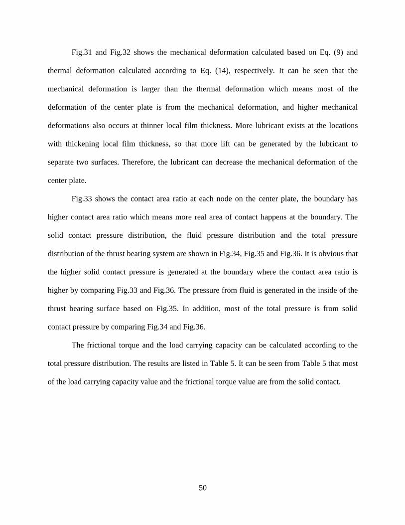
50

Fig.31 and Fig.32 shows the mechanical deformation calculated based on Eq. (9) and

thermal deformation calculated according to Eq. (14), respectively. It can be seen that the

mechanical deformation is larger than the thermal deformation which means most of the

deformation of the center plate is from the mechanical deformation, and higher mechanical

deformations also occurs at thinner local film thickness. More lubricant exists at the locations

with thickening local film thickness, so that more lift can be generated by the lubricant to

separate two surfaces. Therefore, the lubricant can decrease the mechanical deformation of the

center plate.

Fig.33 shows the contact area ratio at each node on the center plate, the boundary has

higher contact area ratio which means more real area of contact happens at the boundary. The

solid contact pressure distribution, the fluid pressure distribution and the total pressure

distribution of the thrust bearing system are shown in Fig.34, Fig.35 and Fig.36. It is obvious that

the higher solid contact pressure is generated at the boundary where the contact area ratio is

higher by comparing Fig.33 and Fig.36. The pressure from fluid is generated in the inside of the

thrust bearing surface based on Fig.35. In addition, most of the total pressure is from solid

contact pressure by comparing Fig.34 and Fig.36.

The frictional torque and the load carrying capacity can be calculated according to the

total pressure distribution. The results are listed in Table 5. It can be seen from Table 5 that most

of the load carrying capacity value and the frictional torque value are from the solid contact.

51

Fig.33 - Contact area ratio at each node on the center plate (fc = 33,300 m-1

, hs = 1 µm, ω = 0.14

rad/s)

Fig.34 - Pressure distribution generated by the solid contact on the center plate (fc = 33,300 m-1

,

hs = 1 µm, ω = 0.14 rad/s)

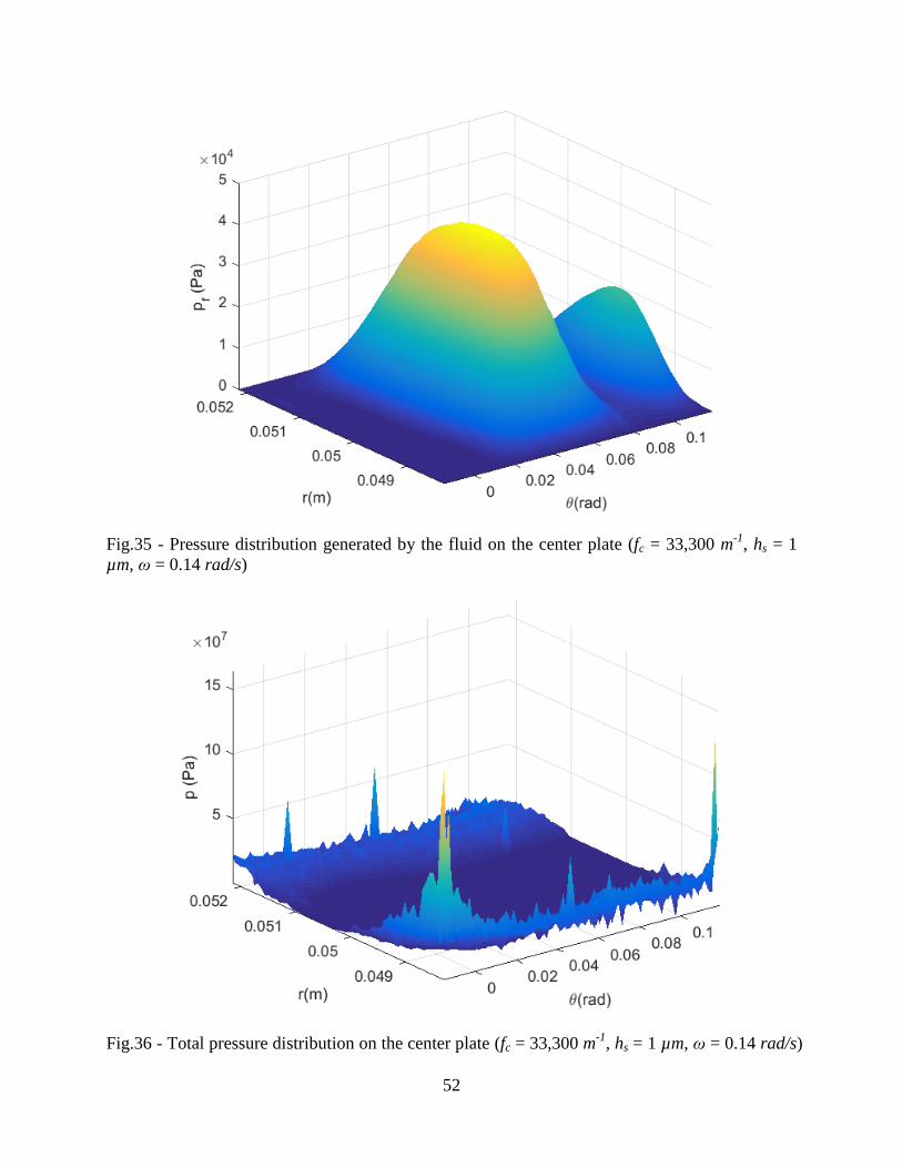
52

Fig.35 - Pressure distribution generated by the fluid on the center plate (fc = 33,300 m-1

, hs = 1

µm, ω = 0.14 rad/s)

Fig.36 - Total pressure distribution on the center plate (fc = 33,300 m-1

, hs = 1 µm, ω = 0.14 rad/s)

53

Table 5 - Values of load carrying capacity and the frictional torque with considering thermal (fc =

33,300 m-1

, hs = 1 µm, ω = 0.14 rad/s)

From

solid contact

From

fluid shearing Total

Percentage from

solid contact

Load carrying capacity, L 5.4496×103 N 9.9495 N 5.4641×10

3 N 99.74%

Frictional torque, T 7.3754 Nm 0.0502 Nm 7.4256 Nm 99.32%

5.2 Results without Consideration of Thermal Effects

For a better comparison, the results of thrust bearing indicators without thermal effects at

the same specific case (fc = 33,300 m-1

, hs = 1 µm, ω = 0.14 rad/s) as considering the thermal

effects are also calculated. The calculated process under this situation is shown in Fig.37. It can

be found by comparing Fig.4 and Fig.37 that the thermal deflection is neglected when the

thermal effects are not considered. Since temperature rise can also influence the viscosity of the

lubricant, the temperature influence on the lubricant is also not considered in this situation.

Fig.38 to Fig.43 show the film thickness distribution, the mechanical deformation, the

contact area distribution, the pressure distribution from solid contact, the pressure distribution

from fluid and the total pressure distribution, separately. All these plots are predicted without

considering the thermal effects.

As we concluded in the situation with considering the thermal influence, the mechanical

deformation happens at the place where the film thickness is thin based on the Figs. 38 and 39.

Fig.40 shows more real area of contact occurs at the boundary.

Meanwhile, the higher pressure is generated at the boundary where the contact area is

higher and most of the total pressure is from solid contact pressure, the same phenomena also

happen for the situation without considering the thermal effects according to Figs. 40 - 43. The

calculated load carrying capacity and frictional torque values for this situation are listed in Table

54

6. It can also be concluded that most of the load carrying capacity and the friction torque are still

generated by the solid contact.

55

Fig.37 - Flow chart of the mixed lubrication calculation without thermal effects

Fig.38 - Film thickness distribution between one pad of the center plate and the upper case

without thermal influence (fc = 33,300 m-1

, hs = 1 µm, ω = 0.14 rad/s)

56

Fig.39 - Mechanical deformation of one pad in the center plate without thermal influence (fc =

33,300 m-1

, hs = 1 µm, ω = 0.14 rad/s)

Fig.40 - Contact area distribution of one pad in the center plate without thermal influence (fc =

33,300 m-1

, hs = 1 µm, ω = 0.14 rad/s)

57

Fig.41- Pressure distribution from solid contact on one pad of the center plate without thermal

influence (fc = 33,300 m-1

, hs = 1 µm, ω = 0.14 rad/s)

Fig.42 - Pressure distribution from fluid on one pad of the center plate without thermal influence

(fc = 33,300 m-1

, hs = 1 µm, ω = 0.14 rad/s)

58

Fig.43 - Total pressure distribution on one pad of the center plate without thermal influence (fc =

33,300 m-1

, hs = 1 µm, ω = 0.14 rad/s)

Table 6 - Values of load carrying capacity and the frictional torque without considering thermal

effects (fc = 33,300 m-1

, hs = 1 µm, ω = 0.14 rad/s)

From

solid contact

From


Percentage from

solid contact


3 N 99.51%


5.3 Comparison of the Results with and without Considering Thermal Effects

For a better comparison of these two situations with and without considering thermal

effects, the relationship between the minimum film thickness (hmin) and the contact area ratio

(A*), the load carrying capacity (Ltotal), the frictional torque (Ttotal), and the ratio for the

contribution of the fluid part and the solid contact part on the load carrying capacity and the

59

frictional torque with the same initial surface separation (hs = 1 µm) are studied. The results are

plotted in Figs. 44 to 48.

Fig. 44 - Relationship between the minimum film thickness (hmin) and the contact area ratio (A*)

for the situations with and without considering thermal influence

60

Fig.45 - Relationship between the minimum film thickness (hmin) and the load carrying capacity

(Ltotal) for the situations with and without considering thermal influence

Fig.46 - Relationship between the minimum film thickness (hmin) and the frictional torque (Ttotal)

for the situations with and without considering thermal influence

61

Fig.47 - Relationship between the minimum film thickness (hmin) and the ratio of the load

carrying capacity from fluid (Lf) and the load carrying capacity from solid contact (Ls)

Fig.48 - Relationship between the minimum film thickness (hmin) and the ratio of the frictional

torque from fluid (Tf) and the frictional torque from solid contact (Ts)

5.4 Results and Discussions

It can be concluded from the Figs. 45 and 46 that the difference between the total load

carrying capacity and the total frictional torque for the situations with and without considering

the thermal influence are very small (the angular velocity considered here is ω = 0.14 rad/s).

According to the trend lines in Figs. 47 and 48, the proportions of the load carrying capacity and

the frictional torque from fluid decrease when the thermal effects are considered during the

analysis. This is because the temperature in the thrust bearing system will increase when the

thermal effects are considered, which will make the viscosity of the lubricant becomes lower.

Therefore, the lift force between two surfaces will become smaller and more solid contact will

happen.

62

Yu and Sadeghi [18] concluded that thermal effects can reduce the load carrying capacity

and the frictional torque. However, the total load carrying capacity and the total frictional torque

do not change too much when considering the thermal effects and the thermal effects only reduce

the load carrying capacity and the frictional torque from fluid. Perhaps this is because the angular

velocity considered here is very low and the thrust bearing is in the mix lubrication regime, most

of the load carrying capacity and the frictional torque are carried by the solid contact. In the work

of Yu and Sadeghi, the bearing they considered is under the hydrodynamic regime and the load

carrying capacity value and the frictional torque value are all generated by the fluid.

The angular velocity is also increased in this work (which will be discussed in Chapter 7),

the thrust bearing will tend to be a hydrodynamic bearing with the increase of the angular

velocity and more load carrying capacity and the frictional torque will be carried by the fluid.

Then the changing trend of the load carrying capacity and the frictional torque will probably

become closer to the analysis of Yu and Sadeghi. Otherwise, the lubricant they used is not the

same as what we used in our experiment, which will also make different changes of the total load

carrying capacity and the total frictional torque.

5.5 Conclusions

In this part, a mixed lubrication thermo-elastic model of a sectored thrust bearing is

created. This model is able to provide predictions of important quantities such as frictional

torque, load carrying capacity, minimum film thickness, temperature rise, contact pressure.

However, this model requires further development verification with the experimental results and

the results from the other existed models.

In addition, for a thrust bearing system under the mixed lubrication regime, more solid

contact will happen when considering the thermal effects and the thermal effects can reduce the

63

load carrying capacity and the frictional torque from fluid when the angular velocity of the thrust

bearing system is small.

Furthermore, the code we programmed for the model can also be used to investigate the

influence of various design parameters on thrust bearing performance.

64

CHAPTER 6

SURFACE CHARACTERIZATION

In Chapter 4, a new thrust bearing model is established and the results are analyzed in

Chapter 5. Even with the existence of the lubricant between two surfaces during the rotation of

thrust bearings, surface asperities can still come into contact to influence the performance of the

thrust bearings. Therefore, the characterization of the rough surface is very important in studying

the thrust bearing system. This chapter focuses more on the surface characterization.

6.1 Measured Surface Fractal Characterization

Fig.49 - Rough surface with 2048 2048 nodes from thrust bearing

65

In this chapter, the rough surface of a single pad with 2048 2048 nodes (46.54% of the

refined pad surface) is chosen from the refined pad surface (see Fig.17) as shown in Fig.49 (the

coordinate values are normalized by the outer radius value of the thrust bearing (ro)), and the

surface data is leveled to make sure the average slope of the surface is zero before calculating the

surface parameters. The reason we choose 2048 2048 nodes on the measured surface is that the

Fast Fourier transform (FFT) method will be used in the analysis, it is the most efficient when

the number of samples is a power of 2. In addition, other common statistical parameters, like root

mean square roughness (Rq), skewness (Sk) and kurtosis (K) as in Table 3 are also calculated for

the chosen rough surface.

Since this chapter is only considered the fractal characterization, the thermal influence is

not considered for the simplification. The calculation process is the same as shown in Fig.37.

The 1-D roughness-length method is used to calculate the fractal dimension of surface

profiles in our previous work [32, 33]. The 3-D roughness-length method [34] (as we illustrated

in Chapter 2) is used here to calculate the fractal dimension value of the measured rough surface

(see Eq. (16)). Fig.50 shows the plot of the roughness-length method [34] in calculating the

fractal dimension value. The calculated fractal dimension value is also listed in Table 9.

As discussed in Chapter 4, the same mapping process and the surface deconstruction

process are conducted on the measured surface shown in Fig.49. Then the film thickness, the

mechanical deformation, the contact area distribution, the solid contact pressure, the fluid

pressure and the total pressure of the measured surface for the specific case (when the cut-off

frequency fc = 33,300 m-1

, the initial surface separation is hs = 1 µm and the angular velocity ω =

0.14 rad/s) is obtained.

66


measured surface

Fig.51 shows the film thickness distribution between the center plate and the upper casing,

the film thickness in the inside of the rough surface is larger than that at the boundary. Fig.52

shows the mechanical deformation of the center plate and Fig.53 shows the contact area ratio of

each node on the center plate. It can be found that the larger the mechanical deformation is, the

higher the contact area ratio happens by comparing Fig.52 and Fig.53.

The solid contact pressure distribution, the fluid pressure distribution and the total

pressure distribution are shown in Fig.54, Fig.55 and Fig.56. According to these three figures,

most of the pressure is carried by the solid contact, and the larger pressure values occur at the

boundary. After the pressure and shear stress are obtained, the frictional torque and load carrying

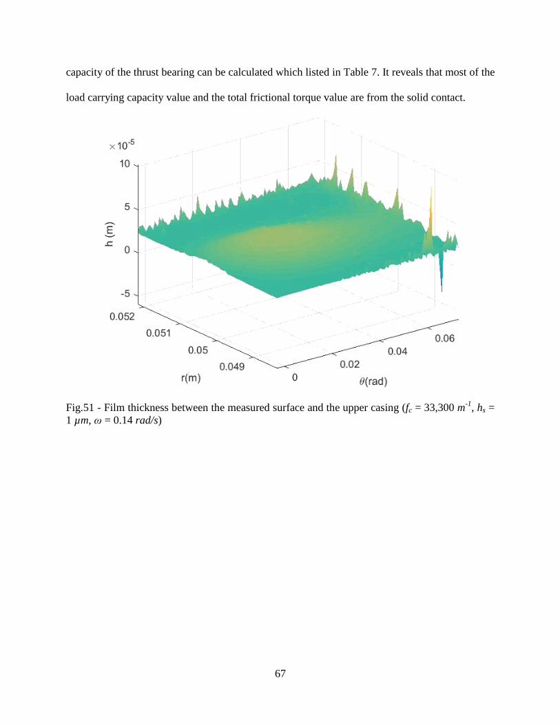
67

capacity of the thrust bearing can be calculated which listed in Table 7. It reveals that most of the

load carrying capacity value and the total frictional torque value are from the solid contact.

Fig.51 - Film thickness between the measured surface and the upper casing (fc = 33,300 m-1

, hs =

1 µm, ω = 0.14 rad/s)

68

Fig.52 - Mechanical deformation of the measured surface (fc = 33,300 m-1

, hs = 1 µm, ω = 0.14

rad/s)

Fig.53 - Contact area ratio on each node of the measured surface (fc = 33,300 m-1

, hs = 1 µm, ω =

0.14 rad/s)

69

Fig.54 - Solid contact pressure distribution on the measured surface (fc = 33,300 m-1

, hs = 1 µm,

ω = 0.14 rad/s)

Fig.55 - Fluid pressure distribution on the measured surface (fc = 33,300 m-1

, hs = 1 µm, ω = 0.14

rad/s)

70

Fig.56 - Total pressure distribution on the measured surface (fc = 33,300 m-1

, hs = 1 µm, ω = 0.14

rad/s)

Table 7 - Values of the load carrying capacity and the frictional torque for the measured surface

(fc = 33,300 m-1

, hs = 1 µm, ω = 0.14 rad/s)

From

solid contact

From


Percentage from

solid contact


3 N 99.21%


6.2 Surface Generation Methods

Two different methods are used to artificially generate rough surfaces with the same fractal

dimension calculated from the measured rough surface. One is the 3D PSD-iFFT method, which

is short for the inverse Fourier transform based on a prescribed Power Spectral Density. The

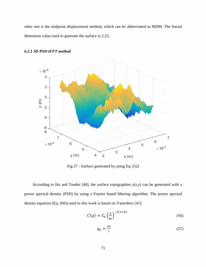
71

other one is the midpoint displacement method, which can be abbreviated as MDM. The fractal

dimension value used to generate the surface is 2.23.

6.2.1 3D PSD-iFFT method

Fig.57 - Surface generated by using Eq. (52)

According to Hu and Tonder [40], the surface topographies z(x,y) can be generated with a

power spectral density (PSD) by using a Fourier based filtering algorithm. The power spectral

density equation (Eq. (60)) used in this work is based on Yastrobov [41]:

𝐶(𝑞) = 𝐶0 (𝑞

𝑞0)−2(1+𝐻)

(56)

𝑞0 =2𝜋

𝑙 (57)

72

where C0 is a constant, q0 is the cut-off wave vector, l is the length of the measured surface. After

the power spectral density (PSD) is calculated by Eq. (56), the surface can be generated by

applying the Hermitian symmetry and the inverse Fourier transform on the obtained PSD (which

is shown in Fig.57). The mapping process and the surface deconstruction process are also

conducted on this PSD generated surface. Some basic parameters and the fractal dimension value

calculated by the roughness-length method [34] for the PSD generated surface are also listed in

Table 8. The plot used in calculating the fractal dimension value is shown in Fig.58.


surface generated by the PSD generated method

Fig.59 to Fig.61 show the film thickness, the mechanical deformation, the contact area

distribution of the PSD generated surface for the same specific case as the measured surface

shown in Fig.49 (fc = 33,300 m-1

, hs = 1 µm, ω = 0.14 rad/s). It can be found by comparing

D = 2.23

73

Fig.59 and Fig.60 that the larger mechanical deformation happens at the place where the film

thickness is smaller. Fig.61 shows that the boundary has higher contact area ratio which means

the real area of contact is larger at the boundary. The larger the contact area ratio is, the higher

the mechanical deformation will be.

Figs. 62 - 64 show the solid contact pressure distribution, the fluid pressure distribution

and the total pressure distribution of the PSD generated surface (fc = 33,300 m-1

, hs = 1 µm, ω =

0.14 rad/s). Same phenomena happen as for the measured surface that most of the pressure is

from solid contact and larger pressure lies at the boundary where the contact area ratio is large.

Then the load carrying capacity and the frictional torque values for the PSD generated surface

can be evaluated (see Table 8 for the values). Again, most of the load carrying capacity and the

frictional torque are generated by the solid contact.

Fig.59 - Film thickness of the PSD generated surface (fc = 33,300 m-1

, hs = 1 µm, ω = 0.14 rad/s)

74

Fig.60 - Mechanical deformation of the PSD generated surface (fc = 33,300 m-1

, hs = 1 µm, ω =

0.14 rad/s)

Fig.61 - Contact area ratio at each node of the PSD generated surface (fc = 33,300 m-1

, hs = 1 µm,

ω = 0.14 rad/s)

75


, hs = 1

µm, ω = 0.14 rad/s)


, hs = 1

µm, ω = 0.14 rad/s)

76

Fig.64 - Total pressure distribution on the PSD generated surface (fc = 33,300 m-1

, hs = 1 µm, ω =

0.14 rad/s)



, hs = 1 µm, ω = 0.14 rad/s)

From

solid contact

From


Percentage from

solid contact


3 N 99.13%


6.2.2 Midpoint displacement method

This surface generation method was first proposed by Fournier et. al. [42] in 1982 and

then discussed by Saupe [43] and Voss [44]. The generated process of this method can be

summarized below (Fig.65 schematically shows the generated process of this method):

77

1) Considering a square in the x-z plane, the height of four corners in the plane is from

the Gaussian distribution N(µ,σ2) ;

2) Picking up the midpoint of the square, the height of the midpoint is the average value

of the four corners plus a Gaussian random number N(0,1) and the fractal dimension value

calculated from the measured surface is also considered;

3) Calculating the height of the midpoint of every side of the square, then the initial

plane can be divided into four new squares;

4) This process is repeated for each new obtained square with the original large squares

until we get the desired surface resolution.

Fig.65 - Generated process of the midpoint displacement method

1） 2）

3）

4）

78

In this process, the expectation of the distribution, µ, and root mean square roughness, σ,

values are all from the measured surface shown in Fig.49. Since the fractal dimension value D =

3-H, the fractal dimension value in step 2) is considered by using the equation below [45]:

𝜎𝑖2 =

1

22𝐻(𝑖+1)𝜎2 (58)

where σi is a modified RMS roughness in the i-th iteration step.

Fig.66 shows the surface generated from the midpoint displacement method (MDM). The

same parameters are calculated for the MDM generated surface and listed in Table 9. The plot

used for calculating fractal dimension value is shown in Fig.67. Again, the same mapping

process and the surface deconstruction process are conducted on this MDM generated surface.

Fig.66 - Surface generated by midpoint displacement method

79

Fig.67 - Plot of the roughness-length method in calculating fractal dimension value for the MDM

generated method

Table 9- Basic parameters calculated for the measured surface, the PSD generated surface and

the MDM generated surface

Parameters Measured surface PSD generated

surface

MDM generated

surface


m 1.2619e×10-5

m 7.0002×10-6

m

Kurtosis (K) 2.8980 7.2189 4.7459

Skewness (Sk) 0.0908 -1.0941 0.0768


m 1.2370×10-5

m 4.6311×10-6

m


m-2

2.6728e×1010

m-2

7.9589×1010

m-2

Fractal dimension (D) 2.23 2.23 2.11

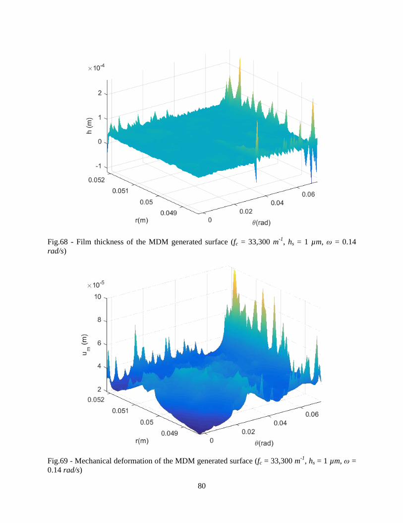
80

Fig.68 - Film thickness of the MDM generated surface (fc = 33,300 m-1

, hs = 1 µm, ω = 0.14

rad/s)

Fig.69 - Mechanical deformation of the MDM generated surface (fc = 33,300 m-1

, hs = 1 µm, ω =

0.14 rad/s)

81

Fig.70 - Contact area distribution of the MDM generated surface (fc = 33,300 m-1

, hs = 1 µm, ω =

0.14 rad/s)

Fig.71 - Solid contact pressure distribution of the MDM generated surface (fc = 33,300 m-1

, hs =

1 µm, ω = 0.14 rad/s)

82

Fig.72 - Fluid pressure distribution of the MDM generated surface (fc = 33,300 m-1

, hs = 1 µm, ω

= 0.14 rad/s)

Fig.73 - Total pressure distribution of the MDM generated surface (fc = 33,300 m-1

, hs = 1 µm, ω

= 0.14 rad/s)

83



, hs = 1 µm, ω = 0.14 rad/s)

From

solid contact

From


Percentage from

solid contact


3 N 99.73%


The film thickness distribution, the mechanical deformation, the contact area distribution,

the solid contact pressure distribution, the fluid pressure distribution and the total pressure

distribution of the MDM generated surface based on the same specific case as the measured

surface are calculated and plotted in Figs. 68 - 73 (fc = 33,300 m-1

, hs = 1 µm, ω = 0.14 rad/s).

Different from the measured surface and the PSD generated surface, some points at the

boundary of the MDM generated surface have higher film thickness according to Fig.68.

However, the larger mechanical deformation and the higher contact area ratio still happen at the

place where the film thickness is thinner by comparing Fig.68, Fig.69 and Fig.70. Most of the

pressure is from the solid contact as for the measured surface and the PSD generated surface

based on the Figs. 71, 72 and 73.

The load carrying capacity and the frictional torque values then can be computed for the

MDM generated surface, which are listed in Table 10 (most of the load carrying capacity and the

frictional torque are generated by the solid contact).

84

Chapter 7

ANALYSIS OF MEASURED AND GENERATED SURFACES

7.1 Influence of the Angular Velocity

It can be found from the pressure distribution results in Chapter 5 and Chapter 6 that the

pressure contribution from the fluid is very small compared to the values from solid contact, so

that the contribution of load carrying capacity from the fluid is also very small for this

application case. As we mentioned previously, these cases are for a relatively low angular

velocity of 0.14 rad/s based on an application of this bearing. Therefore, the influence of angular

velocity at values larger than this on the load carrying capacity and the frictional torque are also

investigated. With the constant cut-off frequency (fc = 33,300 m-1

) and the same initial surface

separation (hs = 30 µm), the angular velocity is changed from 0.14 rad/s to 419 rad/s. Figs. 74

and 77 show the relationships between the total load carrying capacity (Ltotal) and the total

frictional torque (Ttotal) as a function of the angular velocity (ω) for these three surfaces.

The changing trends of the ratio for the contribution of the fluid part and the solid contact

part on the load carrying capacity and the frictional torque with the changing of the angular

velocity (ω) for these three surfaces are shown in Figs. 76 and 79. Figs. 75 and 78 show the

changing trends of the load carrying capacity from the solid contact (Ls) and the frictional torque

from the solid contact (Ts) along with the angular velocity (ω).

85

In addition, the relationship between the contact area ratio (A*) and the angular velocity

(ω) for these three surfaces and the relationship between the minimum film thickness (hmin) and

the angular velocity (ω) are also plotted in Fig.80 and Fig.81, separately.

Fig.74 - Relationship between the total load carrying capacity (Ltotal) and the angular velocity (ω)

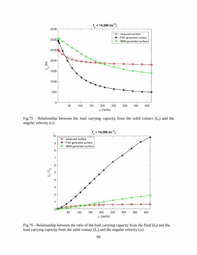
86

Fig.75 - Relationship between the load carrying capacity from the solid contact (Ls) and the

angular velocity (ω)

Fig.76 - Relationship between the ratio of the load carrying capacity from the fluid (Lf) and the

load carrying capacity from the solid contact (Ls) and the angular velocity (ω)

87

Fig.77 - Relationship between the total frictional torque (Ttotal) and the angular velocity (ω)

Fig.78 - Relationship between the frictional torque from the solid contact (Ts) and the angular

velocity (ω)

88

Fig.79 - Relationship between the ratio of the frictional torque from the fluid (Tf) and the

frictional torque from the solid contact (Ts) and the angular velocity (ω)

Fig.80 - Relationship between the contact area ratio (A*) and the angular velocity (ω)

89

Fig.81 - Relationship between the minimum film thickness (hmin) and the angular velocity (ω)

Fig.74 indicates that with the increase of the angular velocity, the load carrying capacity

increases, which is in agreement with typical hydrodynamic bearing behavior. Again note that

the original surface separation is held constant, but the actual surface separation can increase due

to deformation. The slope of the load carrying capacity with speed is the steepest for the PSD

generated surface. The slope of the load for the measured surface is the least. Meanwhile, for the

same angular velocity, the load carrying capacity value from the PSD generated surface is larger

than the other two surfaces when the angular velocity is larger than 20 rad/s.

Fig.75 shows that the load carrying capacity value from the solid contact (Ls) decrease

when the angular velocity becomes larger for these three surfaces. The slope of the decrease

90

speed for the PSD generated surface is the steeper than that for the other two surfaces and the

decrease speed for the generated surface is the least.

The proportion of the load carrying capacity also increases with the growth of the angular

velocity, which means the proportion of the load carrying capacity from fluid has become

significant. The ratio for the MDM generated surface is the smallest at the low angular velocity,

but the ratio (Lf/Ls) from the measured surface becomes the smallest as angular velocity becomes

much larger (Fig.76). It should also be noted from Fig.76 that the ratio (Lf/Ls) for the measured

surface is not larger than one, but the ratio (Lf/Ls) for the other two generated surfaces all become

larger than one with the increase of the angular velocity. It means much of the load is carried

more by the fluid if the ratio (Lf/Ls) is larger than one. This is more desirable for a typical fluid-

film bearing. This may be due to clear differences in the larger scale geometries of the generated

surfaces compared to the measured surface.

The same phenomena have also been predicted for the frictional torque according to Figs.

77, 78 and 79. The frictional torque values from these three surfaces increase with the increase of

the angular velocity, the measured surface increases the most, while the PSD generated surface

increase the least. The frictional torque value from the solid contact (Ls) decreases for these three

surfaces (Ts). Meanwhile, the contribution of the frictional torque from fluid has increased with

the growth of the angular velocity for these three surfaces.

The ratios (Lf/Ls and Tf/Ts) from the PSD generated surface is the largest for all cases. The

proportion of the load carrying capacity and the frictional torque from the fluid increases

significantly with the growth of the angular velocity and becomes much larger than the load

carrying capacity and the frictional torque from solid contact for the PSD generated surface. The

increase of the ratios (Lf/Ls and Tf/Ts) with the angular velocity for the measured surface and the

91

MDM generated surface is much less. The ratios (Lf/Ls and Tf/Ts) from the measured surface

becomes the smallest gradually, which means that the contact area in the measured surface is

larger than the contact area in the other two generated surfaces at the same angular velocity.

According to Fig.80, the contact area ratio for these three surfaces decreases with the

increase of the angular velocity. The PSD generated surface has the highest contact area ratio at

the initial angular velocity, and then it decreases more steeply. When the angular velocity is

larger than 70 rad/s, the contact area ratio for the measured surface becomes the largest. Since

the contact area ratio is a measure of the degree of asperity contact during the rotation, the larger

the contact area ratio is, the larger the real area of contact is. Fig.80 can also illustrate that the

proportion of the load carrying capacity and the frictional torque from the fluid increases with

the increase of the angular velocity.

The minimum film thickness with the deformation (hmin) for the MDM generated surface

is larger than the other two surfaces based on the plot in Fig. 81, but it does not change too much

when the angular velocity (ω) becomes larger. The minimum film thickness with the

deformation (hmin) value for the measured surface decreases when the angular velocity (ω) is

larger than 150 rad/s and then start to increase. For the PSD generated surface, the minimum

film thickness with the deformation (hmin) increases first with the increase of the angular velocity

(ω) and then decrease when the angular velocity is larger than 250 rad/s.

It can be concluded from the analysis above that the angular velocity influences each of

the surfaces differently when comparing the two generated surfaces from the measured surface.

Therefore, the two surface generation methods are not suitable in representing the measured

surface.

92

7.2 Influence of the Cut-off Frequency

In the case we discussed above, the cut-off frequency we used to deconstruct the surface

is fc = 33,300 m-1

(the wavelength, λ, is 30 µm). More cases with different cut-off frequencies are

run for these three different surfaces (the angular velocity is held constant during this process at

ω = 250 rad/s and the initial surface separation hs = 1 µm), and the plots of the relationship

between the cut-off frequency and the total load carrying capacity and the total frictional torque

for these three surfaces are shown in Figs. 82 and 83. The plots of the relationship between the

cut-off frequency (fc) and the total load carrying capacity (Ltotal) and the total frictional torque

(Ttotal) for more cases with different angular velocity (the initial surface separation is held

constant at hs = 1 µm) are shown in Appendix A and Appendix B, separately.

It can be seen from Figs. 82 and 83 that the load carrying capacity value and the frictional

torque value from the two generated surfaces are very large when the cut-off frequency is very

small. Whereas, the load carrying capacity value and the frictional torque value from two

generated surfaces decrease with the increase of the cut-off frequency. Meanwhile, the

predictions of these two values from two generated surfaces become coincident with the values

for the measured surface if the cut-off frequency becomes large enough. The load carrying

capacity and the frictional torque values from the MDM generated surface are much closer to the

values from the measured surfaces than the PSD generated surface. It should also be noted that

the change of the load carrying capacity value and the frictional torque value from the measured

surface is very small with the increase of the cut-off frequency.

93

Fig.82 - Relationship between the total load carrying capacity (Ltotal) and the cut-off frequency (fc)

Fig.83 - Relationship between the total frictional torque (Ttotal) and the cut-off frequency (fc)

94

From the analysis above, when the cut-off frequency used to deconstruct the surface is

small, both of the PSD generated surface and the MDM generated surface are not very suitable in

representing the measured surface. However, these two generated surfaces can represent the

measured surface when the cut-off frequency becomes large. It means that the characterization

ability of the generated surfaces depends heavily on the cut-off frequency.

By comparing the parameter values in Table 8, the Rq values of the measured surface, the

PSD generated surface and the MDM generated surface have little difference. The Sk and K

values for the MDM generated surface are much closer to the measured surface than the PSD

generated surface, but the values of asperity radius and asperity density calculated from the

MDM generated surface are not as consistent as the values calculated by the PSD generated

surface when comparing with the values of the measured surface. Clearly, these two regenerated

fractal surfaces are structured fundamentally different than the measured surface. This will result

in different behavior in the mix-lubrication regime.

It should be noted that both of the two generated surface methods consider the fractal

dimension value when generating the surface, and the generated surfaces based on these two

methods are not consistent in characterizing the measured surface. Therefore, it should be

considered carefully if the generated surface based on the fractal dimension can be used to

represent a measured surface. Due to the differences of the predicted results, the fractal

dimension is not a reliable value to solely characterize the measured surface. However, if other

parameters could be considered in the generation process as well, improvement might be made.

However, since only a few generated surfaces are evaluated due to the computational

limitations, the results cannot be considered generalized.

95

7.3 Influence of the Initial Surface Separation

In this section, the influence of the different initial surface separations (hs) on the

indicators of these three surfaces is investigated with the constant cut-off frequency value (fc =

33,300 m-1

) and the different angular velocity values. Figs. 84 to 98 show the plot of the

relationships between the angular velocity and the contact area ratio, the load carrying capacity,

the frictional torque, Lf/Ls and Tf/Ts with different initial surface separations for the measured

surface, the PSD generated surface and the MDM generated surface.


initial surface separations for the measured surface

96


initial surface separations for the PSD generated surface


initial surface separations for the MDM generated surface

97


different initial surface separations for the measured surface


different initial surface separations for the PSD generated surface

98


different initial surface separations for the MDM generated surface



separations for the measured surface

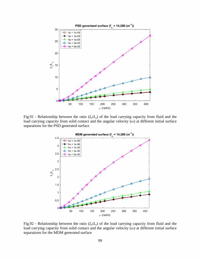
99



separations for the PSD generated surface



separations for the MDM generated surface

100


different initial surface separations for the measured surface


different initial surface separations for the PSD generated surface

101


different initial surface separations for the MDM generated surface



separations for the measured surface

102







103

According to Figs. 84, 85 and 86, the contact area ratio decreases with the increase of the

initial surface separation for the same angular velocity, which means the solid contact between

asperities decreases for these three surfaces, as expected.

As we discussed above, the load carrying capacity, the frictional torque, the ratios (Lf/Ls

and Tf/Ts) all increase with the increase of the angular velocity for these three surfaces. The load

carrying capacity and the frictional torque values decrease with the increase of the initial surface

separation when the same angular velocity value is picked up for these five situations according

to Figs. 87-89 and Figs. 93-95, which means less asperities come into contact when the initial

surface separation becomes large for these three surfaces.

However, the ratios (Lf/Ls and Tf/Ts) increase with the increase of the initial surface

separation for a constant angular velocity according to Figs. 90-92 and Figs. 96-98. Therefore,

the higher the initial surface separation value is set, the more contribution of the fluid for the load

carrying capacity and the frictional torque value provides for these three surfaces.

In addition, the thrust bearing tends to be a hydrodynamic bearing with the increase of the

angular velocity and the same phenomena still have happened when the angular velocity

becomes larger for these three surfaces. Hence, the initial surface separation value can also

influence the performance of a thrust bearing under hydrodynamic lubrication regime.

7.4 Influence of the Small Scale Roughness and Large Scale Roughness

Meanwhile, two new surfaces (surface A and surface B) are also constructed based on the

small scale roughness and the large scale roughness of the measured surface and the PSD

generated surface using the following method (see Figs. 99 and 100):

(1) Surface A: combine large scale roughness from the measured surface with small scale

roughness from the PSD generated surface;

104

(2) Surface B: combine small scale roughness from the measured surface with large scale

roughness from the PSD generated surface.

This analysis allows one to determine which scale of roughness is more important and

which can be generated.

Fig.99 - New generated surface (surface A) based on large scale roughness of the measured

surface data and small scale roughness of the PSD generated surface data

105

Fig.100 - New generated surface (surface B) based on the small scale roughness of the measured

surface data and large scale roughness of the PSD generated surface data

Table 11 - Related parameters calculated for surface A, surface B, the measured surface and the

PSD generated surface

Surface A Surface B Measured surface PSD generated

surface


m 1.2617×10-5

m 1.1074×10-5

m 1.2619e×10-5

m

Kurtosis (K) 2.9026 7.2077 2.8980 7.2189

Skewness (Sk) 0.0941 -1.0911 0.0908 -1.0941


m 1.1096×10-5

m 1.1096×10-5

m 1.2370×10-5

m


m-2

3.5170e×1010

m-2

3.5170×1010

m-2

2.6728e×1010

m-2

Fractal dimension (D) 2.51 2.16 2.23 2.23

106


A


B

107

Table 12 - Some parameters calculated based on different cut-off frequencies

surface A surface B

fc (m-1

) Rq (m) Sk K D Rq (m) Sk K D

5.00e04 1.1067×10-5

0.0939 2.9026 2.5895 Rq (m) -1.0917 7.2096 2.3775

3.33e04 1.1063×10-5

0.0941 2.9026 2.5074 1.2619×10-5

-1.0911 7.2077 2.1587

2.50e04 1.1060×10-5

0.0942 2.9030 2.4358 1.2617×10-5

-1.0906 7.2059 2.1646

2.00e04 1.1057×10-5

0.0944 2.9035 2.4127 1.2615×10-5

-1.0902 7.2043 2.1400

1.67e04 1.1055×10-5

0.0945 2.9037 2.3962 1.2613×10-5

-1.0899 7.2028 2.1235

1.43e04 1.1053×10-5

0.0945 2.9037 2.3713 1.2610×10-5

-1.0897 7.2016 2.1134

1.25e04 1.1051×10-5

0.0945 2.9039 2.3532 1.2607×10-5

-1.0897 7.2017 2.1034

1.11e04 1.1049×10-5

0.0944 2.9043 2.3414 1.2604×10-5

-1.0894 7.2000 2.0810

1.00e04 1.1047×10-5

0.0943 2.9045 2.3414 1.2600×10-5

-1.0896 7.1997 2.0717

5.00e03 1.1039×10-5

0.0924 2.9065 2.3018 1.2596×10-5

-1.0920 7.2059 2.0559

3.33e03 1.1036×10-5

0.0882 2.9008 2.2932 1.2547×10-5

-1.0986 7.2266 2.0620

2.50e03 1.1036×10-5

0.0814 2.8894 2.2816 1.2485×10-5

-1.1041 7.2697 2.0648

2.00e03 1.1042×10-5

0.0745 2.8700 2.2799 1.2411×10-5

-1.1253 7.2823 2.0725

1.67e03 1.1045×10-5

0.0647 2.8484 2.2848 1.2324×10-5

-1.1428 7.2957 2.0900

1.43e03 1.1049×10-5

0.0532 2.8149 2.2826 1.2235×10-5

-1.1562 7.5180 2.1101

1.25e03 1.1061×10-5

0.0310 2.7518 2.2869 1.2090×10-5

-1.2293 7.7008 2.1328

1.11e03 1.1061×10-5

0.0310 2.7518 2.2869 1.1898×10-5

-1.2293 7.7008 2.1328

1.00e03 1.1082×10-5

-0.0035 2.6532 2.2870 1.1898×10-5

-1.2700 7.8841 2.2058

5.00e02 1.1479×10-5

-0.1753 2.7466 2.2768 1.1601×10-5

-1.6790 11.685 2.2861

3.33e02 1.1479×10-5

-0.1753 2.7466 2.2768 8.9553×10-5

-1.6790 11.685 2.2861

108

Small scale roughness and large scale roughness are determined based on the cut-off

frequency. Surface A and surface B shown in Figs. 99 and 100 are generated when the cut-off

frequency is 33,300 m-1

. For these two shown surfaces, the same basic parameters and the fractal

dimension value from the roughness-length method [34] are calculated (see Table 11). Fig.101

and Fig.102 show the plots of the roughness-length method in calculating the fractal dimension

value for these two combined surfaces. Table 12 shows the basic parameters and the fractal

dimension value for surface A and surface B with different cut-off frequencies.

The measured surface and surface A have similar values of Rq, Sk and K, and the values

of Rq, Sk and K for the PSD generated surface and surface B are similar based on Table 11,

which means large scale roughness tends to dominate the calculation process of the statistical

parameters.

By changing the initial surface separation and the cut-off frequency (angular velocity

keeps constant) of the measured surface, the PSD generated surface, surface A, and surface B,

the changing trend between the cut-off frequency and the total load carrying capacity and the

total frictional torque for some cases are plotted (see Fig.103 and Fig.104), the other cases are

shown in Appendix C and Appendix D.

109

Fig.103 - Changing trend between the minimum film thickness (hmin) and the total load carrying

capacity (Ltotal)

110

Fig.104 - Changing trend between the minimum film thickness (hmin) and the total frictional

torque (Ttotal)

When the cut-off frequency is smaller, the values of the load carrying capacity and the

frictional torque predicted by the PSD generated surface are smaller than the values from the

measured surface according to Fig.103 and Fig.104. With the growth of the cut-off frequency,

the load carrying capacity value and the frictional torque value become larger than the values

calculated from the measured surface.

As we mentioned above, the small scale roughness of surface A is from the PSD generated

surface and the small scale roughness of surface B is from the measured surface. The trend lines

111

of the total load carrying capacity and the frictional torque for the measured surface and surface

B are very close, and the trend lines for the PSD generated surface and surface A are the same.

Therefore, the small scale roughness appears to be dominant in the mixed lubrication regime.

In addition, it is important to understand the physical meaning of the different values of

the fractal dimension when discussing the results. According to Majumdar and Bhushan [46], the

surface fractal dimension (Ds) can be related to the profile fractal dimension (Dp) by using Ds =

1+Dp. It has already been shown in our previous work [32, 33] that the fractal dimension value

for a self-similar surface profile is 1. Therefore, the fractal dimension for a self-similar surface

should be 2. Note that a surface profile is one line of a 3-D surface.

By comparing the fractal dimension value in Table 8 and Table 10, it can be seen that the

measured surface, the PSD generated surface, the MDM generated surface and surface B tend to

be self-similar. Nonetheless, the parameter values listed in Table 11 is based on the specific case

(fc = 33,300 m-1

), different cut-off frequencies are changed to verify the influence of cut-off

frequency on some parameters listed in Table 11 and the values are listed in Table 12.

It can be found from Table 12 that the values of Rq, K and Sk for surface A and surface B

do not change significantly with the changing of the cut-off frequency, except at low cut-off

frequencies, which are near to the macro scale geometry and would not typically be used (see

Figs. 105, 106 and 107). It can be found from Fig.105 that the Rq value for surface A decreases

with the increase of the cut-off frequency, and the Rq value for surface B increase with the

growth of the cut-off frequency. At larger cut-off frequency, the decrease speed for surface A

and the increase speed for surface B slow down. The Sk value for both of surface A and surface

B increase with the increase of the cut-off frequency according to Fig.106, the slope of the

changing line becomes smaller and smaller as the increase of the cut-off frequency. Different

112

from the changing trend of Rq value for surface A and surface B, K value for surface A increase

and K value for surface B decrease with the growth of the cut-off frequency based on Fig.107.

Similarly, the changing speed of K value for both of these two surfaces becomes slow down

when the cut-off frequency becomes large.

However, the fractal dimension value is influenced significantly by the changing of the

cut-off frequency. Fig.108 shows the relationship between the cut-off frequency and the fractal

dimension value for surface A and surface B based on Table 12.

Fig.105 - Relationship between the cut-off frequency (fc) and the RMS roughness (Rq)

113

Fig.106 - Relationship between the cut-off frequency (fc) and the Skewness (Sk)

Fig.107 - Relationship between the cut-off frequency (fc) and the Kurtosis (K)

114

Fig.108 - Relationship between the cut-off frequency (fc) and the fractal dimension (D)

According to Fig.108, fluctuation happens in the fractal dimension value with the

increase of the cut-off frequency. It can be concluded by comparing Figs. 105-108 that fractal

dimension actually varies more than roughness or statistical values with scale, which means that

the fractal dimension depends on the chosen cut-off frequency and it is not always a reliable

parameter in characterizing the rough surface.

7.5 Conclusions

The shear rate of the fluid increases with the increase of the angular velocity, so that the

shear stress increases. As a result, the load carrying capacity and the frictional torque values

from the real surface, the PSD generated surface and the MDM generated surface all increase but

115

at different amounts. The proportions of the load carrying capacity and the frictional torque from

fluid have also increased for the measured surface, the PSD generated surface and the MDM

generated surface with the growth of the angular velocity. However, the ratios (Lf/Ls and Tf/Ts)

from the PSD generated surface has been the largest for all angular velocities and the ratios (Lf/Ls

and Tf/Ts) from the measured surface becomes the smallest for larger angular velocities.

Therefore, when the angular velocity increases large enough, the contact area of the measured

surface is larger than the other two generated surfaces at the same angular velocity value. This

suggests that the angular velocity has a greater influence on the two generated surfaces and that

the two surface generation methods are not suitable in representing the measured surface.

When the cut-off frequency used in deconstructing the surface is small, the PSD

generated surface is relatively better in representing the measured surface. Whereas, when the

cut-off frequency becomes larger, the MDM generated surface can represent the measured

surface better, but they both represent the measured surface poorly.

The load carrying capacity value and the frictional torque value calculated for the

measured surface, the PSD generated surface and the MDM generated surface are not the same

and the load carrying capacity ratio from the fluid and from the solid contact for these three

surfaces increases differently, which means it should be considered carefully whether generated

surface based on the fractal dimension can be used to represent a measured surface. It should be

mentioned again that only a few generated surfaces are evaluated due to the computational

limitations, therefore the results cannot be considered generalized.

Meanwhile, this work suggests that the fractal dimension is unreliable when it is the only

parameter to characterize the measured surface since the results for the fractal surface and the

measured surface differ significantly and it also changes with the chosen angular velocity and

116

cut-off frequency. It should also be noted that the small scale roughness is dominant in the mixed

lubrication regime and large scale roughness affects a lot in the calculation process of the

statistical parameters.

Although the input parameters for the generated rough surfaces are from the measured

rough surface, some surface properties changed during the generation procedure, which implies

that the surface generation methods we used in our work need to be improved and new methods

need to be developed.

117

Chapter 8

SURFACE OPTIMIZATION

8.1 Optimization Process

It has been concluded that the small scale roughness is the dominant part of the geometry

in the mixed lubrication regime from Chapter 7. The influence of the large scale geometry on the

load carrying capacity is investigated in this chapter. The objective of this chapter has been to

maximize the load carrying capacity from the fluid (Lf) on a surface by combining the small

scale roughness from the measured surface and the large scale geometry from a designed

equation. Based on the shape of the measured surface in Fig.49, the large scale geometry

equation might be approximated as:

𝑧𝑙𝑎𝑟𝑔𝑒 = (𝑎𝜃2 + 𝑏𝜃 + 𝑐) × (𝑑𝑟2 + 𝑒𝑟 + 𝑓) (59)

where a, b, c, d, e and f are constants. These six unknowns can be represented by two unknowns

when the following boundary conditions below are applied:

𝑧𝑙𝑎𝑟𝑔𝑒(𝑟, 𝜃0) = 𝑧𝑙𝑎𝑟𝑔𝑒(𝑟, 𝜃1)=0 (60)

𝑧𝑙𝑎𝑟𝑔𝑒(𝑟𝑖, 𝜃) = 𝑧𝑙𝑎𝑟𝑔𝑒(𝑟𝑜 , 𝜃)=0 (61)

where 𝜃0 and 𝜃1 are angles at two boundaries of the thrust bearing in the circumferential

direction; 𝑟𝑖 and 𝑟𝑜 are the inner and outer radius of the thrust bearing. In these two boundary

conditions, the height at four edges of the thrust bearing is set to be zero.

By applying these boundary conditions and set b = e, Eq. (59) can be written as:

𝑧𝑙𝑎𝑟𝑔𝑒 = (−14.2526𝑏𝜃2 + 𝑏𝜃 + 0.0031𝑏) × (−9.9509𝑏𝑟2 + 𝑏𝑟 − 0.0251𝑏) (62)

118

Fig.109 shows the plot of the large scale geometry (b = 5) generated by Eq. (62). Fig.110

shows the optimized surface by combining the small scale roughness from the measured surface

with the large scale geometry generated by Eq. (62). During the optimization process, the cutoff

frequency is kept consistent for the small scale roughness from the measured surface and large

scale geometry from Eq. (62), which is fc = 14,286 m-1

.

During the numerical process for the new combined surface, the total load carrying

capacity is kept constant while the average film thickness is allowed to vary for a better

investigation of the large scale geometry. Therefore, a load balance is required in the code. The

numerical calculation process with the load balance part is used which is shown in Fig.111. It

should be noted that the temperature influence part is neglected in this numerical process so that

computational time can be reduced.

Fig.109 - Large scale geometry generated by Eq.(62) (b = 5, fc = 14,286 m-1

)

119

Fig.110 - Sample of generated surface (b = 5, fc = 14,286 m-1

)

120

Fig.111 - Flow chart of calculation process with load balance

121

Fig.112 - Flow chart of optimization process

Fig.112 shows the flow chart of the entire optimization process. Since b is the only

unknown in Eq. (62), b is set to an initial value of 1 with an increment 1 in this optimization

process (the cutoff frequency is 14,286 m-1

and the initial surface separation is 1 μm in this

process). By using the load balance calculation process in Fig.111, the load carrying capacity

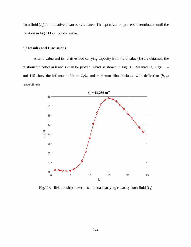
122

from fluid (Lf) for a relative b can be calculated. The optimization process is terminated until the

iteration in Fig.111 cannot converge.

8.2 Results and Discussions

After b value and its relative load carrying capacity from fluid value (Lf) are obtained, the

relationship between b and Lf can be plotted, which is shown in Fig.113. Meanwhile, Figs. 114

and 115 show the influence of b on Lf/Ls and minimum film thickness with deflection (hmin)

respectively.

Fig.113 - Relationship between b and load carrying capacity from fluid (Lf)

123

Fig.114 - Relationship between b and the ratio between the load carrying capacity from fluid (Lf)

and the load carrying capacity from solid contact (Ls)

Fig.115 - Relationship between b and minimum film thickness with defection (hmin)

124

It can be found from Fig.113 that when b = 15, the load carrying capacity from the fluid

(Lf) has the largest value which means the surface can be optimized. However, this is not the

optimal value, but is close to it. The proportion of the load carrying capacity from fluid increases

with the increase of the b value, and it decreases when the b value becomes larger than 15

according to Fig.114. In addition, Fig.115 shows the changing trend of the minimum film

thickness with deflection (hmin) is the same as the changing trend of the load carrying capacity

from the fluid (Lf). Therefore, the larger the film thickness is, the more hydrodynamic part the

thrust bearing has and the more load carrying capacity generated by the fluid.

Fig.116 shows the nearly optimized surface shape when b = 15. It should be note that the

scale of the height is amplified, the actually height of the surface feature is small compared to the

lengths of the lateral edges.

Fig.116 - Optimized surface shape when b = 15 (fc = 14,286 m-1

)

125

8.3 Conclusions

In this chapter a large scale geometry equation is derived which is used to generate an

nearly optimized surface. An optimized surface is constructed by adding small scale roughness

from the measured surface and large scale geometry from the large scale geometry equation. It

can be found that when the unknown, b, in the large scale geometry equation equals to 15, the

optimized surface can generate the largest load carrying capacity from fluid when the total load

carrying capacity, the cut-off frequency and the initial surface separation are held constant.

Therefore, the thrust bearing surface in this study can be optimized to improve the tribological

performance.

However, most of surface optimization process is focused on the journal bearings [47-49]

or the stepped shaped thrust bearings [50] and not too many works focused on the flat thrust

bearings, this optimization process need to be improved by finding more models about the flat

thrust bearing surface advanced optimization algorithm.

126

CHAPTER 9

CLOSURE

9.1 Conclusions

In this work, a mixed lubrication bearing model is proposed and used to evaluate

different realizations of the same surface. This new model is able to provide predictions of

important quantities such as frictional torque, load carrying capacity, minimum film thickness,

temperature rise, and contact pressure.

The angular velocity and the cut-off frequency all have a great influence on the PSD and

the MDM generated surfaces, and the surface parameters used in the two surface generation

methods are not suitable in characterizing the measured surface. Therefore, it should be

considered carefully if the generated surface based on the fractal dimension can be used to

represent a measured surface. Meanwhile, the fractal dimension is unreliable when it is the only

parameter to characterize the measured surface since it changes with the cut-off frequency, and

real measured rough surfaces are not easily represented as perfect fractals as researchers and

engineers often assume,

9.2 Contributions

The contributions of this work to the tribology and engineering filed can be summarized

as:

127

1) Mixed lubrication problems (Reynolds equation) and rough surface contact (GW

model) with roughness are solved and the influence of the surface roughness on the lubricant

behavior is shown.

2) Generated roughness surfaces by fractal methods cannot be used to represent the real

surface.

3) Fractal dimension is not a reliable parameter as researches often regarded.

4) Surface geometry can be optimized.

9.3 Future Work

The model built can make predictions of the performance indicators for the thrust bearing

system. However, it still requires further development and verification by comparing with some

other existing models and experimental measurements. In addition, the periodic boundary

condition is the only boundary condition we considered. Additional boundary conditions, such as

cavitation boundary condition, will be added in our model in the future to improve the

predictions.

The lubricant we used in our work is grease, which is a non-Newtonian fluid as we

discussed. However, the Reynolds equation used in this work is more often used for Newtonian

fluids [27] which can only make an approximate prediction of the hydrodynamic part when the

lubricant is grease. Therefore, an improvement of the model needs to be made by finding a

generalized Reynolds equation that can be used in the grease EHL in the cylindrical coordinates.

Since the fractal dimension value is not a reliable parameter in characterizing rough

surfaces it is necessary to find new parameters to characterize the real rough surfaces.

Although the input parameters for the generated rough surfaces are from the measured

rough surface, some surface properties changed during the generation procedure, which implies

128

that the surface generation methods we used in our experiment need to be improved and new

methods need to be developed.

In addition, the surface geometry optimization process in this work needs to be improved

by finding more algorithms and comparing with more models on the flat thrust bearing

optimization.

129

REFERENCE

[1] Shi, F., Wang, Q., ‘‘A Mixed-TEHD Model for Journal-Bearing Conformal Contacts—Part I:

Model Formulation and Approximation of Heat Transfer Considering Asperity Contact,’’ ASME

Journal of Tribology, 120, pp. 198–205, 1998;

[2] Shi, F., Wang, Q., ‘‘A Mixed-TEHD Model for Journal-Bearing Conformal Contacts—Part II:

Contact and Performance Analyses,’’ ASME Journal of Tribology, 120, pp. 206–213, 1998;

[3] Zhang, C. “TEHD Behavior of Non-Newtonian Dynamically Loaded Journal Bearings in

Mixed Lubrication for Direct Problem,’’ ASME Journal of Tribology, 124, pp. 178-185, 2002;

[4] Muzakkir, S. M., Hirani, h., and Thakre, G. D., “Experimental Investigations on

Effectiveness of Axial and Circumferential Grooves in Minimizing Wear of Journal Bearing

Operating in Mixed Lubrication Regime,” International Journal of Current Engineering and

Technology, 5(1), pp. 486-489, 2015;

[5] Raimondi, A. A., Boyd J., “A Solution for the Finite Journal Bearing and its Application to

Analysis and Design: III”,ASLE Transactions, 1, 1, pp.194-209, 1958;

[6] Gao, G., Yin, Z., Jiang, D., and Zhang, X., “Numerical analysis of plain journal bearing

under hydrodynamic lubrication by water”, Tribology International, 75, pp. 31-37, 2014;

[7] Kirk, R. G., Funter, E. J., “Short Bearing Analysis Applied to Rotor Dynamics—Part I:

Theory”, ASME Journal of Lubrication Technology, 98, 1, pp. 47-56, 1976;

[8] Sun, J., Gui, C. “Hydrodynamic lubrication analysis of journal bearing considering

misalignment caused by shaft deformation”, Tribology International, 97, 10, pp.841-848, 2004;

130

[9] McCallion, H., Yousif, F., and Lioyd, T., “The Analysis of Thermal Effects in a Full Journal

Bearing”, ASME Journal of Lubrication Technology, 92, 4, pp. 578-587, 2010;

[10] Prakash, J., Vij, S. K., “Analysis of Narrow Porous Journal Bearing Using Beavers-Joseph

Criterion of Velocity Slip”, ASME Journal of Applied Mechanics, 41, 2, pp. 348-354, 1974;

[11] Bouyer, J., Fillon, M., “An Experimental Analysis of Misalignment Effects on

Hydrodynamic Plain Journal Bearing Performances”, ASME Journal of Tribology, 124, 2, pp.

313-319, 2001;

[12] Brockwell, K., Ettles, C., and Stokes, M., “A Design Method for Radially Grooved Thrust

Washers”, Proceedings of the Institution of Mechanical Engineers, 184, pp. 82-92, 1969;

[13] Heshmat, H., Walowit, J. A., and Pinkus, O., “Analysis of Gas Lubricated Compliant Thrust

Bearings”, ASME Journal of Lubrication Technology, 105, 4, pp. 638-646, 1983;

[14] Carpino, M., “Analysis of a Low Speed Flexible Flat Land Thrust Bearing”, ASME Journal

of Tribology, 112, 4, pp. 678-683, 1990;

[15] Yu, T.H., Sadeghi, S., “Groove Effects on Thrust Washer Lubrication”, ASME Journal of

Tribology, 123, 2, pp.295-304, 2000;

[16] Cameron, A., Wood, W. L., “Parallel Surface Thrust Bearing”, ASLE Transactions, 1, 2,

pp.254-258, 1958;

[17] Taniguchi, S., Ettles, C., “A Thermo-Elastic Analysis of the Parallel Surface Thrust

Washer”, ASLE Transactions, 18, 4, pp. 299-305, 1976;

[18] Yu, T.H., Sadeghi, S., “Thermal Effects in Thrust Washer Lubrication”, ASME Journal of

Tribology, 124, 1, pp.166-177, 2001;

[19] Jackson, R. L., Green, I., “The Behavior of Thrust bearings Considering Mixed Lubrication

and Asperity Contact”, Tribology Transactions, 49, 2, pp.233-247, 2006;

131

[20] Jackson, R.L., Green, I., “The Thermoelastic Behavior of Thrust bearings Considering

Mixed Lubrication Asperity Contact and Thermoviscous Effects”, Tribology Transactions, 51, 1,

pp.19-32, 2008;

[21] Jackson, R.L., Green, I., “Study of the Tribological Behavior of a Thrust bearing”,

Tribology Transactions, 44, 3, pp.504-508, 2001.

[22] Mandelbrot, B.B., “The fractal geometry of nature”, Macmillan, New York, NY, 1983;

[23] Mandelbrot, B.B., “Self-affine fractal sets, I: the basic fractal dimensions”, Fractals in

Physics, 3, pp.3-15, 1986;

[24] Patir, N., Cheng, H.S., “An Average Flow Model for Determining Effects of Three-

Dimensional Roughness on Partial Hydrodynamic Lubrication,” ASME Journal of Tribology,

100, 1, pp. 12-17, 1978;

[25] Patir, N., Cheng, H.S., “Application of Average Flow Model to Lubrication Between Rough

Sliding Surfaces,” ASME Journal of Tribology, 101, 2, pp. 220-230, 1979;

[26] Greenwood, J.A., Williamson, J.B.P., “Contact of Nominally Flat Surface”, Proceedings of

the Royal Society A, 295, 1442, pp. 300-319, 1966;

[27] Kazama, T., Yamaguchi, A., “Application of a Mixed Lubrication Model for Hydrostatic

Thrust Bearing of Hydraulic Equipment”, ASME Journal of Tribology, 115, 4, pp.686-691, 1993;

[28] Guo, Y., Lu, X., and Li, W., et. al., “A mixed-lubrication model considering elastoplastic

contact for a piston ring and application to a ring pack”, Journal of Automobile Engineering, 229,

2, pp. 174-188, 2015.

[29] Love, A. E. H., “Stress Produced in a Semi-infinite Solid by Pressure on Part of the

Boundary”, Philosophical Transactions of Royal Society, 228, 659-669, pp. 377- 420, 1929;

[30] Johnson, K. L., “Contact Mechanics”, Cambridge University Press, 1985;

132

[31] Barber, J. R., “Effect of Thermal Distortion on Constriction Resistance”, International

Journal of Heat and Mass Transfer, 14, 6, pp. 751-766, 1971b;

[32] Zhang, X., Jackson, R.L., “An Analysis of the Multiscale Structure of Surfaces with Various

Finishes”, Tribology Transaction, 60, 1, 121-134, 2017;

[33] Zhang, X., Xu, Y., and Jackson, R.L., “An Analysis of Generated Fractal and Measured

Rough Surfaces in Regards to Their Multi-scale Structure and Fractal Dimension”, Tribology

International, 105, pp. 94-101, 2017;

[34] Fardin, N., Stephansson, O., and Jing, L., “The Scale Dependence of Rock Joint Surface

Roughness”, International Journal of Rock Mechanics and Mining Sciences, 38, 5, pp.659-669,

2001;

[35] Hamrock, B. J., “Fundamentals of Fluid Film Lubrication”, McFraw-Hill, Inc., Hightstown,

NJ, 1994;

[36] Roelands, C.J.A., “Correlational aspects of the viscosity-temperature-pressure relationship

of lubricating oils”, Druk. V.R.B, Groningen, 1966;

[37] Özisik, M. N., “Heat Conduction”, 2nd edition, New York: John Wiley, 1993;

[38] Khayat, K. H., Yahia, A., “Effect of Welan Gum-high-range Water Reducer Combinations

on Rheology of Cement Grout”, ACI Materials Journal, 94, 5, pp. 365-372, 1997;

[39] Jackson, R. L., Green, I., “Experimental Analysis of the Wear, Life and Behavior of PTFE

Coated Thrust bearing under Non-axisymmetric Loading”, Tribology Transactions, 46, 4, pp.

600-607, 2003;

[40] Hu, Y. Z., Tonder, K., “Simulation of 3-D Random Rough Surface by 2-D Digital Filter and

Fourier Analysis”. International Journal of Machine Tools and Manufacture, 32, pp.83–90, 1992;

133

[41] Yastrebov, V.A., Anciaux, G., Molinari, J., “From Infinitesimal to Full Contact Between

Rough Surfaces: Evolution of the Contact Area”, International Journal of Solids and Structures,

52, pp.83-102, 2015.

[42] Fournier, A., Fussell, D., and Carpenter, L., “Computer Rendering of Stochastic Models”,

Graphics and Image Processing, 25, 6, pp.371-384, 1982.

[43] Saupe, D., “Algorithms for Random Fractals”, In: Barnsley, M.F., Devaney, R.L.,

Mandelbrot, B.B., Peitgen, H.-O., Saupe, D., Voss, R.F. (Eds), The Science of Fractal Images.

Springer, New York, pp. 71-136, 1988.

[44] Voss, R.F., “Fractal in Nature: From Characterization to Simulation”, In: Barnsley, M.F.,

Devaney, R.L., Mandelbrot, B.B., Peitgen, H.-O., Saupe, D., Voss, R.F. (Eds), The Science of

Fractal Images. Springer, New York, pp. 21-70, 1988.

[45] Marak, I., http://old.cescg.org/CESCG97/marak/node3.html;

[46] Majumdar, A., Bhushan, B., “Fractal Model of Elastic-plastic Contact Between Rough

Surfaces”, ASME Journal of Tribology, 113, 1, pp.1-11, 1991.

[47] Yang, B.S., Choi, B.K., and Kim, H.J., 2001, “Optimum Design of Short Journal Bearings

by Atificial Life Algorithm,” Tribology International, 34, pp. 427-435;

[48] Hirani, H., 2004, “Multiobjective optimization of a journal bearing using the Pareto

optimality concept,” Proceedings of the institution of Mechanical Engineers, Part J: Journal of

Engineering Tribology, 218, pp. 323- 336;

[49] Pang, X., Qin, N., and Dwyer-Joyce, R.S., et. al., 2010, “A General Profile Parameterization

of Hydrodynamic Journal Bearings for Efficient Shape Optimization,” Tribology Transactions,

53, pp. 117-126;

134

[50] Fesanghary, M., Khonsari, M.M., 2012, “Topological and Shape Optimization of Thrust

Bearings for Enhanced Load-carrying capacity,” Tribology International, 53, pp.12-21;

135

APPENDICES

A: Relationship between the load carrying capacity and the cut-off frequency for different

angular velocity

Fig.A1 - Relationship between the load carrying capacity (Ltotal) and the cut-off frequency (fc) for

different angular velocity (ω)

136

B: Relationship between the frictional torque and the cut-off frequency for different

angular velocity

Fig.B1 - Relationship between the total frictional torque (Ttotal) and the cut-off frequency (fc) for

different angular velocity (ω)

137

C: Changing trend between the cut-off frequency and the total load carrying capacity

138

Fig.C1 - Changing trend between the cut-off frequency (fc) and the total load carrying capacity

(Ltotal)

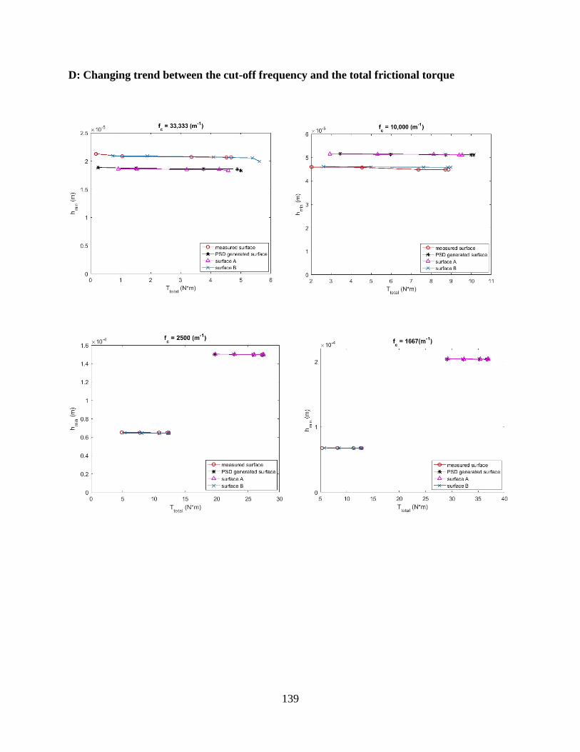
139

D: Changing trend between the cut-off frequency and the total frictional torque

140

Fig.D1 - Changing trend between the cut-off frequency (fc) and the total frictional torque (Ttotal)

Documents

An Analysis of Surface Roughness and its Influence on a