Sc&ce of Coinputer Programming 3 ( 1983) 205-2 16 North-Hollarfd

205

AN ALTERNATIVE FOR THE IMPLEMENTATION OF KRUSKAL’S MINIMAL SPANNING TREE ALGORITHM

Jyrki KATAJAINEN and Olli NEVALAINEN Department of Mathematical Sciences, Unicersity of Turku, Turku, Finland

Communicated by J. Nievergelt Received August 1982 Revised December 1982

Abstract. An application of the bucket sort in Kruskal’s minimal spanning tree algorithm is proposed. The modified algorithm is very fast if the edge costs are from a distribution which is close to uniform. This is due to the fact that the sorting phase then takes for an m edge graph an O(m) average time. The O(m log m) worst case occurs when there is a strong peak in the distribution of the edge costs.

1. Introduction

Let G = (N, E) be an undirected connected graph, N being the set of vertices and E the set of edges. Further let E’r E. Then the subgraph T = (N, E’) of G is a spanning free of G if and only if T is a tree. Let us suppose that a cost or weight c(e) is associated with each edge e E E. The minimal spanning tree problem is then to find a spanning tree T, for which the sum of the costs

C(T) =.;=c(e)

is minimal. In the following we denote n = INI (the number of vertices in the graph) and m = lE[ (the number of the edges).

The implementation of the well-known minimal spanning tree algorithm of Kruskal [7] is discussed in this paper. The impulse to this study arose from the work of Haymond, Jarvis and Shier [6] who gave an efficient implementation of Prim’s algorithm. The so-called address calculation sort [9] is used in their algorithm to aid the selection of new candidate edges to be included in the spanning tree. The experimental tests are promising for the algorithm but it contains the limitation that the edge costs are (or must be mapped to) natural numbers from a limited range.

In the present paper we show how a distribution dependent sort method can be used also in Kruskal’s algorithm. Instead of the address calculation sort we shall use the hybrid sorting technique discussed by Meijer and Akl [ll]. The technique is more general than the former one and strong theoretical results on the average time complexity are available [l].

0167-6423/83/$3.00 @ 1983, Elsevier Science Publishers B.V. (North-Holland)

206 J. Katajainen. 0. Necalainen

The overall plan of the paper is to give a description of the new algorithm in Section 2; to consider the time complexity of the average and worst cases in Section 3; and to give some experimental results in Section 4. Finally in Section 5 we shortly describe the application of hybrid sorting techniques in other graph problems.

2. A modified Kruskal’s algorithm

Kruskal’s minimal spanning tree algorithm uses the greedy method where the

edges are considered in increasing order of the costs and included in the set T of the selected edges if the edges in T do not form a cycle also after the possible inclusion. The step of selecting an edge is repeated until n - 1 edges are included in T. Then T forms the wanted minimal spanning tree of G. The basic fcrm of the above algorithm is the following [7]:

procedure Kruskal:

{This program constructs the minimal spanning tree T for a connected n-vertex graph G(N, E)} begin

l-:=0;’

while ) TI < n - 1 do begin

Select an edge e’ of lowest cost from E;

Delete e’ from E;

if T u {e’} does not contain a cycle then T:= T u {e’}; end;

end.

The choosing of an edge of lowest cost is usually accomplished by forming a min-heap of the edge costs. Thus the sorting of all edges can possibly be avoided. Determining whether the inclusion of a candidate edge would create a cycle in T can be seen as a UNION-FIND problem and it can be solved for example by using one of the possible tree structures as the data structure in the algorithm. One such is the algorithm which makes Quick Merge with Weighting rule in UNION and Collapsing rule in FIND (abbreviated hereafter QMWC) [7].*

’ 0 denotes an empty data structure and also an empty set. ’ The data structure used to represent a subset of vertices, forming a connected component of T. is

a rooted tree, the root being a special vertex of the subset. Let T(i) denote the tree that currently contains the vertex i. Let i and j be two vertices of N. The QMWC-algorithm performs UNION- and FIND-operations as follows:

FIND(i) (Determine the connected component containing the vertex i): Move along the father links to root(T(i)). After this apply the collapsing rule: if j is a node on the path from i to root(T(i)) then set father(i):=roor(T(i)).

UNION(i,j) (Join the connected components containing the vertices i and j): Find root(T(i)) and root(T(j)). Then apply the weighting rule: if the number of nodes in T(j) is less than the number in I(i), make root(T(i)) the father of roor(T(j)). Otherwise make root(T(j)) the father of root(T(i)).

An implementation of Kruskal’s minimal spanning tree algorithm 207

Let us take another look at the search for the minimal edges. Denote by min and ma.r the minimal and maximal edge costs and suppose that both are finite. We divide the range [mm, max] into b intervals of equal length and give the intervals the indexes 1,2,. . . , 6. The edge e, the cost of which is c(e), is associated with the bucket j(e ), where

The edges belonging to the same interval j form a bucket denoted by E(j). In the minimal spanning tree algorithm we first group the edges of E into buckets by the above formula. Thus instead of one large set E of the edges we now have a partitioning E = E(1) u E(2) u * * * u E(b) of it. If the distribution of the edge costs is sufficiently close to uniform, the number of empty buckets is not large.

When choosing the minimal cost edges, the first non-empty bucket E(j) among the buckets E(l), E(2), . . . , E(b) is considered; a min-heap H(j) of the edge costs is constructed for E(j); minimal elements are removed from the heap and added to the spanning forest until the heap becomes empty or the minimal spanning tree T is ready. In the first case the next non-empty bucket is searched for and the same selection process is repeated.

The above gives a new form for Kruskal’s algorithm:

procedure Our-Kruskal: begin

Determine the minimal and maximal costs of the edges in E;

Group the edges of E into buckets E(l), E(2), . . . , E(b); T:=0;

Put each vertex of N into a singular set; j:=O; H(j):=@;

while ITI < n - 1 do begin if H(j) = 0 then begin

Select the next j for which the bucket E(j) is non-empty; Form a heap H(j) for E(j);

end; Select the minimal cost edge e’ = (u, o) from E(j);

Delete e’ from H(j); if FIND(u) #FIND(u) then begin

T:=Tu{e’}; UNION(FIND(u), FIND(u));

end; end;

end.

A clearcut method to form the buckets is to link the elements, describing the edges, in the same bucket to form a linear list and to use an array of list heads

208 J. Katajainen. 0. Nevalainen

which point to the front of the lists. Note that this is not the only possible storage

organization. One could for example count the edges in each bucket and then

reorganize them according to the counts, cf. the method of Math Sort [5]. It is also

possible to arrange the edges by making a chain of exchange operations, see [ 121.

There is more than one way of processing with the min-heaps. Firstly, when

constructing a min-heap of a new bucket it is unnecessary to include into the bucket

an edge which will cause a cycle in a connected component constructed so far. The

appearance of a cycle can again be recognized by performing the FIND-operations

for the two end points of the edge. In the following we suppose that the edges

forming cycles are excluded at the moment of constructing the heaps.

Secondly, let us consider the operation of removing the smallest edge from the

current heap. Here the edge appearing as the last element of the heap is moved

to the place of the element just removed and then moved down to its right position

in the heap. Kershenbaum and Van Slyke [S] considered a single heap-organization

and proposed an improvement for this operation: when removing the last edge it

is checked whether it would form a cycle in the current forest. In that case they

delete the edge and consider the next last element. In our algorithm the use of

buckets aims at the creation of several small heaps. Although the technique of

Kershenbaum and Van Slyke is theoretically appealing our tests indicated that it

increases the total overhead at least for uniformly distributed costs. Thus we have

not implemented it in our algorithm. However, the algorithm is only ca. 4 percent

faster than if the technique were in use. So, the technique of Kershenbaum and

Van Slyke would be advantageous in the case where the distribution of the edge

costs is very irregular.

3. Analysis

Let us first consider the running time of min-heap operations while constructing

the heaps and removing the candidate edges. It may happen that almost all edges

hit a single bucket and the last edge which will be added to T is the very largest

one in E. Then there exists a very big heap from which all elements are to be

removed. Thus in the worst case the time used fur selecting the edges is 0( m log m ) which is the same as when sorting by heapsort. This is true also for the original

Kruskal’s algorithm.

The expected running time used for the heap operations depends on the distribu-

tion of the edge costs. It was shown in [ 111 that the bucket sorting technique works

in O(m) time for uniformly distributed random numbers and for a wide class of

smooth distributions. (It is demanded that the distribution function f(x) of the edge

costs fulfils the conditions: f(x ) = 0 for x & [p, 41 where 4 and p are is fixed and f (x ) is finite. A still wider class of distributions is given in [3].) In the selection of the

edges we essentially sort a subset of the edges by bucket sort and thus for these

distributions the expected selection time is O(m).

An implementation of Kruskal’s minimal spanning tree algorithm 209

Let us next take a look at the FIND- and UNION-operations. We supposed that these are done by the QMWC-algorithm. It has been shown [13] that if t(m’, n) denotes the worst case time required to process an intermixed sequence of m’ 2 n FINDS and n - 1 UNIONS then

for some positive constants kl and kz. Here (Y (m’, n) is a very slowly increasing function for which i sa(m’, n) c 3 for all practical values of m’ and n. Now we have m’s4m because the initialization of the heaps is preceeded by at most 2m

FINDS and possibly we have to remove all m edges from the heaps. Thus the worst

case running time of the QMWC-algorithm in Kruskal’s method is still almost linear on m.

The question on the average running time of the QMWC-algorithm in a minimal spanning tree algorithm seems to be difficult. The sequence of operations when introducing new edges to the spanning forest determines the growth of the subsets and if we want to determine the average running time we must fix the set of graphs for which we are solving the problem.

Yao analyzed in [ 161 several UNION-FIND algorithms in the case of the so-called random spanning tree model. He estimates the running time of a sequence of the equivalence operations “i =j”, which means an operation of the form

“if FIND(i) # FIND(j) then UNION(i, j)“.

He defines the distribution of the input sequence by defining an ensemble f of instruction sequences and assuming that every sequence in f is equally likely to occur:

r={(il=jl, i2=j2,. . . , i,-1 =jn-dl the edges (il, id, (it, jd, . . . , (b-l, in-d

form a spanning tree on the vertices {1,2,. . . , n}}.

Then the QMW (the Quick Merge with Weighting rule) and thus also QMWC runs in an expected O(n) time. But now if m, the number of edges in the graph, is n - 1 the spanning tree found in this way is also minimal. In the special case that additionally the edge costs are from a smooth distribution with short tails, the modified Kruskal’s algorithm runs in an expected O(m) time.3

3 Yao has also studied another model, called the random graph model, to make the equivalence operations. Here a sequence of distinct random edges are introduced into the graph consisting initially of n vertices and none edges. Knuth and Schijnhage [lo] have shown that for the QFW-algorithm (Quick Find with Weighting rule, where the sets are linearly linked lists) the average running time to do the UNION-operations until the graph is connected is O(n). Thus the result can be interpreted as a spanning tree of a complete graph if the edges which form a cycle are rejected. On the other hand Yao has shown that the average running time of QFW and QMW is the same for this model when m = n - I but the case of a complete graph is not explicitly treated. Thus the average running time of the QMWC-algorithm remains undetermined for a general m.

210 J. Katajainen, 0. Necalainen

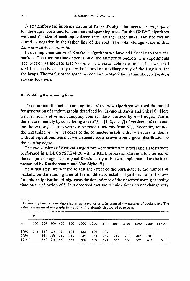
A straightforward implementation of Kruskal’s algorithm needs a storage space for the edges, costs and for the minimal spanning tree. For the QMWC-algorithm we need the size of each equivalence tree and the father links. The size can be stored as negative in the father link of the root. The total storage space is thus 2m+m+2n+n=3m+3n.

In our implementation of Kruskal’s algorithm we have additionally to form the buckets. The running time depends on 6, the number of buckets. The experiments (see Section 4) indicate that b = m/10 is a reasonable selection. Then we need m/10 list heads, an array of m links, and an auxiliary array of the length m for the heaps. The total storage space needed by the algorithm is thus about 5. lm + 3n storage locations.

4. Profiling the running time

To determine the actual running time of the new algorithm we used the model for generation of random graphs described by Haymond, Jarvis and Shier [6]. Here we first fix n and m and randomly connect the n vertices by n - 1 edges. This is done incrementally by considering a set S(j) = {1,2, . . . , j} of vertices and connect- ing the vertex j + 1 to a vertex k selected randomly from S(j). Secondly, we add the remaining m -(n - 1) edges to the connected graph with n - 1 edges randomly without repetitions. Finally, we associate costs drawn from a given distribution to the existing edges.

The two versions of Kruskal’s algorithm were written in Pascal and all tests were performed in a DECSYSTEM-20 with a KLlO processor during a low period of the computer usage. The original Kruskal’s algorithm was implemented in the form presented by Kershenbaum and Van Slyke [8].

As a first step, we wanted to test the effect of the parameter 6, the number of buckets, on the running time of the modified Kruskal’s algorithm. Table 1 shows for uniformly distributed edge costs the dependence of the observed average running time on the selection of 6. It is observed that the running times do not change very

Table 1 The running times of our algorithm in milliseconds as a function of the number of buckets (61. The

values are means of ten graphs (n = 200) with uniformly distributed edge costs

b

m 100 200 400 600 800 1000 1200 1600 2000 2400 4800 9600 14400

1990 146 137 136 134 135 133 136 139

9950 368 358 357 360 359 364 369 367 373 385 401

17910 627 576 563 563 566 569 571 585 587 595 616 627

An implementation of Kruskal’s minimal spanning tree algorithm 211

radically when changing 6. A selection b = m/10 seems to be reasonable and we use this in what follows. When sorting uniformly, normally or negative exponentially distributed random numbers the best selection of b was ca. 5 [12]. This result is in sound with the results of Table 1: in Kruskal’s algorithm some of the edges are deleted already at the time when constructing a heap. Thus the heaps are in many cases smaller than the buckets from which they originate.

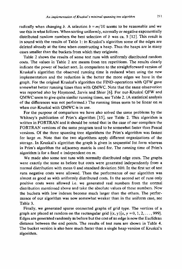
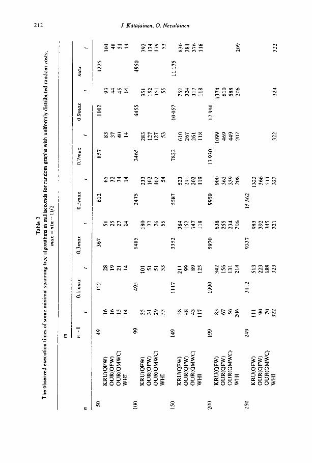
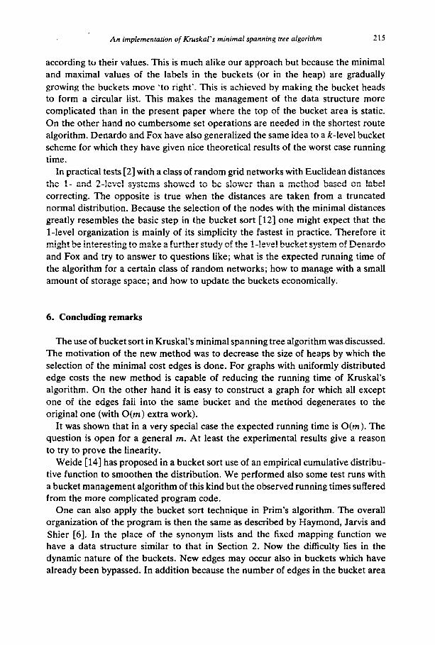
Table 2 shows the results of some test runs with uniformly distributed random costs. The values in Table 2 are means from ten repetitions. The results clearly indicate the power of bucket sort. In comparison to the straightforward version of Kruskal’s algorithm the observed running time is reduced when using the new implementation and the reduction is the better the more edges we have in the graph. For the original Kruskal’s algorithm the FIND-operations with QFW gave somewhat better running times than with QMWC. Note that the same observation was reported also by Haymond, Jarvis and Shier [6]. For our-Kruskal QFW and QMWC seem to give quite similar running times, see Table 2. (A statistical analysis of the differences was not performed.) The running times seem to be linear on m

when our-Kruskal with QMWC is in use. For the purpose of comparison we have also solved the same problems by the

Whitney’s publication of Prim’s algorithm [15], see Table 2. This algorithm is written in FORTRAN and it should be noted that in the case of our compilers the FORTRAN versions of the same program tend to be somewhat faster than Pascal versions. Of the three spanning tree algorithms the Prim’s algorithm was fastest for large m. Note that the two algorithms apply different organizations of the storage. In Kruskal’s algorithm the graph is given in sequential list form whereas in Prim’s algorithm the adjacency matrix is used for. The running time of Prim’s algorithm is for a fixed n independent on m.

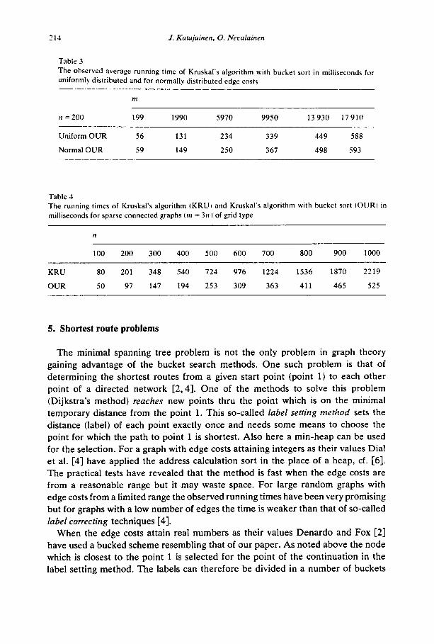
We made also some test tuns with normally distributed edge costs. The graphs were exactly the same as before but costs were generated independently from a normal distribution with mean 0 and standard deviation 500. In the first set of test runs negative costs were allowed. Then the performance of our algorithm was almost as good as with uniformly distributed costs. In the second set of runs only positive costs were allowed i.e. we generated real numbers from the normal distribution mentioned above and take the absolute values of these numbers. NOW the buckets with low indexes become much larger than the others. The perfor- mance of our algorithm was now somewhat weaker than in the uniform case, see Table 3.

Finally, we generated sparse connected graphs of grid type. The vertices of a graph are placed at random on the rectangular grid {(x, y) Ix, y = 0, 1,2, . . . ,999). Edges are generated randomly as before but the cost of an edge is now the Euclidean distance between the end points. The results of test runs are shown in Table 4. The bucket version is also here much faster than a single heap version of Kruskal’s algorithm.

Tab

le

2

The

ob

serv

ed

exec

utio

n tim

es

of s

ome

min

imal

sp

anni

ng

tree

al

gori

thm

s in

mill

isec

onds

fo

r ra

ndom

gr

aphs

w

ith

unif

orm

ly

dist

ribu

ted

rand

om

cost

s;

max

=n(n

-I)/

2

m

n

n-1

0.1

max

0.

3max

0.

5max

0.

7max

0.

9max

m

a*

/ t

t r

I t

I

50

100

150

200

2.50

KR

U(Q

FW

) 16

OU

RtQ

FW

) 16

OU

R(Q

MW

C)

15

WH

I 14

99

KR

UtQ

FW

) 35

OU

R(Q

FW)

31

OU

R(Q

MW

C)

29

WH

I 53

149

KR

U(Q

FW)

OU

R(Q

FW

) O

UR

(QM

WC

)

WH

I

58

48

43

117

199

KR

U(Q

FW

) 83

OU

RtQ

FW

) 67

OU

R(Q

MW

C)

56

Will

20

6

249

KR

U(Q

FW)

Ill

OU

R(Q

FW)

90

OU

R(Q

MW

C)

70

WH

I 32

2

49

122

367

612

857

1102

12

25

28

51

65

83

93

IO1

19

25

32

37

44

48

21

27

34

40

45

51

14

14

14

14

I4

I4

495

1485

24

75

3465

44

55

4950

101

180

233

283

351

392

51

77

102

127

152

I74

51

76

102

127

I.51

I7

9

53

55

54

53

55

53

1117

33

52

5587

78

22

IO05

7 11

17

5 21

1 38

4 52

3 6

IO

752

830

99

152

211

267

324

3x1

89

147

202

261

317

376

125

118

119

118

118

118

1990

59

70

9950

13

930

17

910

342

638

900

1099

13

74

156

255

362

469

610

I31

234

339

449

588

214

206

20X

20

7 20

6 20

9

3112

03

37

IS 5

62

513

983

1322

223

392

566

I88

345

511

323

321

323

322

324

322

300

350

400

450

500

299

KRUQFW

137

OU

R(Q

FW

) 10

9

OU

R(Q

MW

C)

84

WH

I 46

4

KR

UtQ

FW

) O

UR

tQF

W)

OU

R(Q

MW

C)

WI-

11

349

399

449

499

175

139 98

KR

UtQ

FW

) O

UR

tQF

W)

OU

R(Q

MW

C)

WH

I

197

155

112

KR

U(Q

FW)

OU

R(Q

FW

) O

UR

(QM

WC

)

WH

I

250

200

126

KR

U(Q

FW

) O

UR

(QF

W)

OU

R(Q

MW

C)

WH

I

28-3

225

141

4485

13

455

719

1370

315

557

238

499

464

462

6107

953

405

304

18 3

22

1766

7980

1202

510

383

10 1

02

1531

679

467

12 4

75

1855

791

582

465

461

461

460

KR

U

= K

rusk

al’s

al

gori

thm

OU

R

= K

rusk

al’s

al

gori

thm

w

ith

buck

et

sort

WH

I =

Whi

thne

y’s

publ

icat

ion

[15]

of

Pr

im’s

al

gori

thm

QFW

=

Set

oper

atio

ns

mad

e by

Qui

ck

FIN

D

with

W

eigh

ting

rule

in

the

IJ

NIO

Ns

QM

WC

=

Set

oper

atio

ns

mad

e by

Q

uick

M

erge

w

ith

Wei

ghtin

g ru

le

in t

he

UN

ION

S an

d C

olla

psin

g ru

le

in t

he

FIN

DS

214 J. Kalajainen, 0. Necalainen

Table 3

The observed average running time of Kruskal’s algorithm with bucket sort in milliseconds for

uniformly distributed and for normally distributed edge costs

m

n=200 199 1990 5970 9950 13 930 17910

Uniform OUR 56 131 234 339 449 588

Normal OUR 59 149 250 367 498 593

Table 4

The running times of Kruskal’s algorithm (KRUI and Kruskal’s algorithm with bucket sort IOUR, in

milliseconds for sparse connected graphs (m = 3n h of grid type

n

100 200 300 400 500 600 700 800 900 1000

KRU 80 201 348 540 724 976 1224 1536 1870 2219

OUR 50 97 147 194 253 309 363 411 465 525

5. Shortest route problems

The minimal spanning tree problem is not the only problem in graph theory gaining advantage of the bucket search methods. One such problem is that of determining the shortest routes from a given start point (point 1) to each other point of a directed network [2,4]. One of the methods to solve this problem (Dijkstra’s method) reaches new points thru the point which is on the minimal temporary distance from the point 1. This so-called label setting method sets the distance (label) of each point exactly once and needs some means to choose the point for which the path to point 1 is shortest. Also here a min-heap can be used for the selection. For a graph with edge costs attaining integers as their values Dial et al. [4] have applied the address calculation sort in the place of a heap, cf. [6]. The practical tests have revealed that the method is fast when the edge costs are from a reasonable range but it may waste space. For large random graphs with edge costs from a limited range the observed running times have been very promising but for graphs with a low number of edges the time is weaker than that of so-called label correcring techniques [4].

When the edge costs attain real numbers as their values Denardo and Fox [2] have used a bucked scheme resembling that of our paper. As noted above the node which is closest to the point 1 is selected for the point of the continuation in the label setting method. The labels can therefore be divided in a number of buckets

An implementation of Kruskal’s minimal spanning tree algorithm 215

according to their values. This is much alike our approach but because the minimal and maximal values of the labels in the buckets (or in the heap) are gradually

growing the buckets move ‘to right’. This is achieved by making the bucket heads to form a circular list. This makes the management of the data structure more complicated than in the present paper where the top of the bucket area is static. On the other hand no cumbersome set operations are needed in the shortest route algorithm. Denardo and Fox have also generalized the same idea to a k-level bucket scheme for which they have given nice theoretical results of the worst case running time.

In practical tests [2] with a class of random grid networks with Euclidean distances the l- and 2-level systems showed to be slower than a method based on label correcting. The opposite is true when the distances are taken from a truncated normal distribution. Because the selection of the nodes with the minimal distances greatly resembles the basic step in the bucket sort [12] one might expect that the l-level organization is mainly of its simplicity the fastest in practice. Therefore it might be interesting to make a further study of the l-level bucket system of Denardo and Fox and try to answer to questions like; what is the expected running time of the algorithm for a certain class of random networks; how to manage with a small amount of storage space; and how to update the buckets economically.

6. Concluding remarks

The use of bucket sort in Kruskal’s minimal spanning tree algorithm was discussed. The motivation of the new method was to decrease the size of heaps by which the selection of the minimal cost edges is done. For graphs with uniformly distributed edge costs the new method is capable of reducing the running time of Kruskal’s algorithm. On the other hand it is easy to construct a graph for which all except one of the edges fall into the same bucket and the method degenerates to the original one (with O(m) extra work).

It was shown that in a very special case the expected running time is O(m). The question is open for a general m. At least the experimental results give a reason to try to prove the linearity.

Weide [14] has proposed in a bucket sort use of an empirical cumulative distribu- tive function to smoothen the distribution. We performed also some test runs with a bucket management algorithm of this kind but the observed running times suffered from the more complicated program code.

One can also apply the bucket sort technique in Prim’s algorithm. The overall organization of the program is then the same as described by Haymond, Jarvis and Shier [6]. In the place of the synonym lists and the fixed mapping function we have a data structure similar to that in Section 2. Now the difficulty lies in the dynamic nature of the buckets. New edges may occur also in buckets which have already been bypassed. In addition because the number of edges in the bucket area

216 J. Kafujainen, 0. Nevalainen

varies it is difficult to determine an appropriate value for the parameter b. We implemented also this variation and used in the tests the parameter value b = n/2. For very sparse graphs the bucket version of Prim’s algorithm was the fastest of the algorithms studied in this paper whereas for dense graphs it gave very weak

results.

References

r11

Dl

I31

r43

[51 (61

iI bl

PI

INI

fW

WI

[I31 r141

r151 [161

S.G. Akl and H. Meijer, On the average-case complexity of ‘bucketing’ algorithms, J. Aigorithms 3 (1982) 9-13. E.V. Denardo and B.L. Fox, Shortest-route methods: 1, reaching, pruning and buckets, Operations Res. 27(l) (1979) 161-186. L. Devroye and T. Klincsek, Average time behavior of distributive sorting algorithms, Compuring 26(l) (1981) 1-7. R. Dial, F. Glover, D. Karney and D. Klingman, A computational analysis of alternative algorithms and labeling techniques for finding shortest path trees, Networks 9 (1979) 2 15-248. W. Feurzeig, Algorithm 23: Math sort, Collected algorithms from ACM. R.E. Haymond, J.P. Jarvis and D.R. Shier, Computational methods for minimum spanning tree problems, Technical Report # 354, Department of Mathematical Science, Clemson University (1980). E. Horowitz and S. Sahni, Fundamentals of Computer Algorithms (Pitman, Potomac, MD, 1978). A. Kershenbaum and R. Van Slyke, Computing minimum spanning trees efficiently, Pruc. 25ch Annual Conference of the ACM (1972) 518-527. D.E. Knuth, The Art of Computer Programming, Volume I: Fundamental Algorithms (Addison- Wesley, Reading, MA, 1973). D.E. Knuth and A. Schonhage, The expected linearity of a simple equivalence algorithm, Theoret. Compur. Sci. 6 (1978) 281-315. H. Meijer and S. G. Akl, The design and analysis of a new hybrid sorting algorithm, Information Processing Let?. IO(4) (1980) 213-218. 0. Nevalainen and J. Ernvall, Implementation of a distributive sorting algorithm, Department of Mathematical Sciences, University of Turku, Finland (198 1). R. Tarjan, Efficiency of a good but not linear set union algorithm, J. ACM 22(2) (1975) 215-225. B.W. Weide, Statistical methods in aIgorithm design and analysis, Ph.D. Thesis, Carnegie-Mellon University (1978). V.K.M. Whitney, Aigorithm 422: Minimal spanning tree, Comm. ACM 15 (4) (1972) 273-274. A.C. Yao, On the average behavior of set merging algorithms, Proc. 8th Annual Symposium on Theory of Computing (1976) 192-195.