Embed Size (px)
Citation preview
304
REFERENCES
I. F. Netterberg. Calcrete in Road Construction. Council on Scientific and Industrial Research Report RR 286, National Institute for Road Research Bulletin 10. Pretoria, South Africa , 1971 .
2. R. L. Mitchell. Flexible Pavement Design in Zimbabwe. Proc., Institution of Civil Engineers, Part I, 12, London, Aug. 1982, pp. 333-354.
3. A Guide to the Structural Design of Bitumen-Surfaced Roads in Tropical and Sub-Tropical Countries. Road Note 31. Department of Transport, Transport and Road Research Laboratory, HM Stationery Office, London, 1977.
4. J. R. Hosking and L. W. Tu bey. Research on Low-Grade and Unsound Aggregates. Laboratory Report LR 293. Department of Transport, Transport and Road Research Laboratory, Crowthorne, England, 1969.
5. Standard Methods of Testing Road Construction Materials. TM HI. National Institute for Transport and Road Research, Council on Scientific and Industrial Research, Pretoria, South Africa, 1979.
6. Methods of Test for Soils for Civil Engineering Purposes. BS 1377. British Standards Institution, London , 1975.
7. l'vfethodsfor Sampling and Testing of A1inera! Aggregate!s, Sands and Fillers. BS 812 (three parts). British Standards Institution, London. 1975.
Transportation Research Record I 106
8. S. J. Emery. Prediction of Pavement Moisture Content in Southern Africa. Proc., 8th Regional Conference for Africa on Soil Mechanics and Foundation Engineering, Vol. I, Harare, Zimbabwe, 1984, pp. 239-250.
9. H. R. Smith and C. R. Jones. Measurement of Pavement Deflections in Tropical and Sub-Tropical Climates. Laboratory Report 935. Transport and Road Research Laboratory, Crowthorne, England, 1980.
I 0. S. W. A baynayaka. Calibrating and Standardising Road Roughness Measurements Made With Response Type Instruments. Proc., International Conference on Roads and Development, Paris, May 22-25, 1984, (Presses de l'ecole national des pants et chaussees), pp. 13-18.
11. A Guide to the Measurement of Axle Loads in Developing Countries Using a Portable Weighbridge. Road Note 40. Department of Transport, Transport and Road Research Laboratory, HM Stationery Office, London, 1978.
i 2. C. j_ Lawrance and I. Toole. '/he Location, Selection and Use of Calcrete for Bituminous Road Construction in Botswana. Laboratory Report 1122. Department of Transport, Transport and Road Research Laboratory, Crowthorne, England, 1984.
13. Structural Design of Interurban and Rural Road Pavements. Draft TRH 14. National Institute for Transpori and Road Research, Council on Scientific and Industrial Research, Pretoria, South Africa, 1980.
An Aggregate Thickness Design That Is Based on Field and Laboratory Data BERNARD 0. ALKIRE
A summary is provided of the results of a research p'rogram sponsored by the Federal Highway Administration entitled "Design and Operation of Aggregate-Surfaced Roads." Major emphasis is devoted to correlating field and laboratory data and developing the Clegg Impact device as an alternative method for determining in-place density and strength evaluation. Twelve sites in Michigan, Iowa, Texas, Oregon, North Dakota, Montana, West Virginia, and South Carolina were selected for tests. The determination of sites included a variety of climatic and subgrade conditions to allow these factors to be included in the analysis. Field data collected at each field site included roadway dimensions, thickness of the aggregate surface, Clegg Impact Values, in-place density, and moisture content. Bag samples of subgrade and surface aggregate were collected for laboratory tests that included classification tests, gradation, durability, abrasion tests, Clegg Impact Value, and California Bearing Ratio (CBR). Results from laboratory and field tests
Michigan Technological University, Houghton, Michigan 49931.
were analyzed to develop relationships between the various test parameters. A regression analysis of laboratory results showed good agreement between Clegg Impact Value and CBR. The relationship that was developed compared with the results given by Clegg in his work. Statistical relationships that related surface and subgrade conditions in the field to Clegg Impact Value and field moisture content were also obtained and were related to the equation for aggregate thickness design. A discussion that relates the results to the design of low-volume, aggregate-surfaced roads is included.
Millions of miles of roads in the United States are aggregate surfaced. In most cases they have relatively low traffic levels and depend on inexpensive design, construction, and maintenance. Maximum use of local materials and empirical procedures that are based on experience are required to minimize cost.
The results discussed in this paper were collected as part of a project to develop a design procedure for aggregate-surfaced
ALKIRE
roads that includes a consideration of traffic and climate. In developing the design procedure, information on the state of the practice in the design and operation of aggregate-surfaced roads was collected. This involved field visits to 12 locations around the continental United States. The locations that were selected covered a variety of conditions and were chosen to establish a data base on aggregate-surfaced roads that considered climati;:, surface mixtures, thickness, and maintenance. Part of this project involved the collection of field data related to road conditions, dimensions, and materials. This required field tests at the site as well as laboratory tests on samples taken at the field site.
The information collected during the field visit was used to develop a simple design procedure for aggregate-surfaced roads. The design procedure is related to results from the field and laboratory tests on the aggregates.
TESTS
Sites within the continental United States were selected to obtain field data relative to existing practices in the design and operation of aggregate-surfaced roads. At each site, the project personnel talked with a local contact, who was usually a county engineer, but in several areas the contacts were state highway engineers or National Forest Service engineers. The contacts at each site provided basic information about the area and general engineering practices related to aggregate-surfaced roads. The first field visits were made in the summer of 1984. Follow-up visits to most of the sites were made in the spring of 1985:'
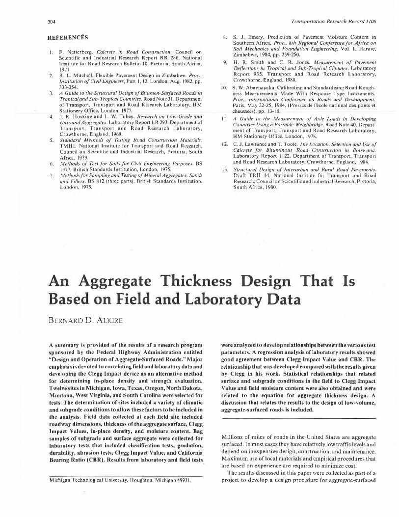
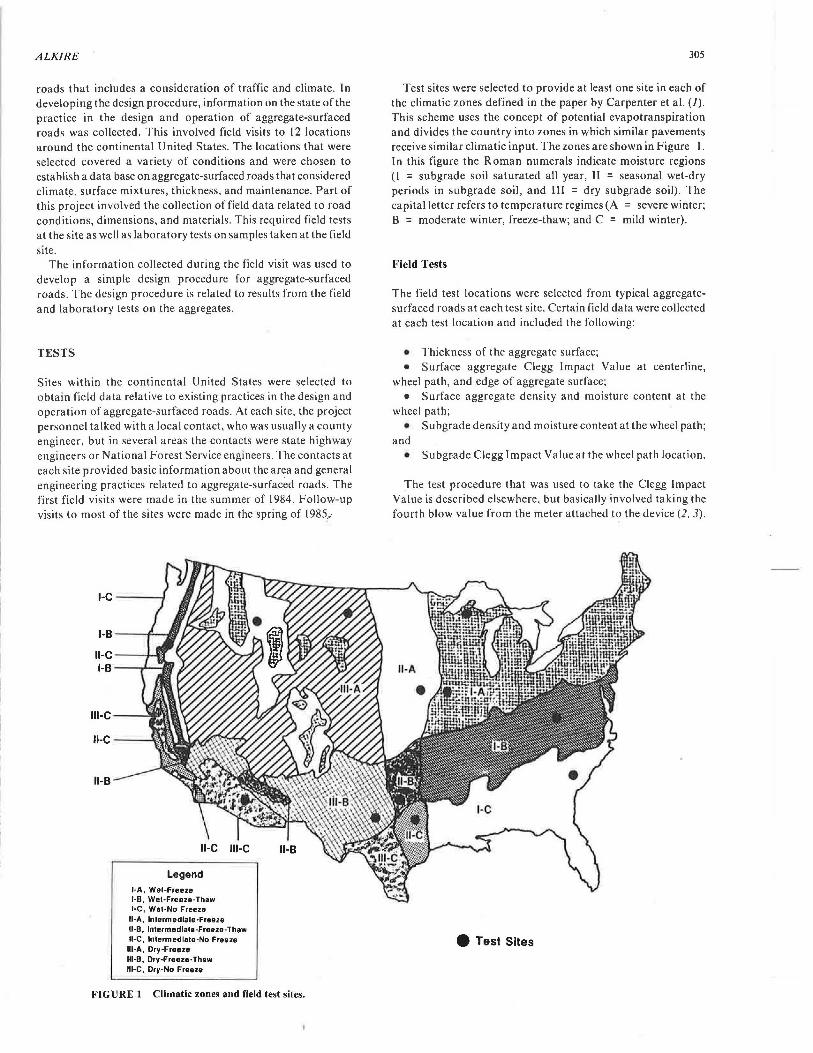
1-B ---r--..1w
11-C ---1Hi:t
1-8 ---......_--
11-B
11-C
Legend I-A, Wei-Freeze 1-B, Wei-Freeze-Thaw 1-C, Wei-No Freeze
II-A, lnlermedlale-Freeze 11-B, lnlermedlale-Freeze-Thew 11-C, lntermedlale-No Freeze
111-A, Dry-Freeze 111-B, Dry-Freeze-Thaw 111-C, Ory-No Freeze
FIGURE 1 Climatic zones and field test sites.
305
Test sites were selected to provide at least one site in each of the climatic zones defined in the paper by Carpenter et al. (1). This scheme uses the concept of potential evapotranspiration and divides the country into zones in which similar pavements receive similar climatic input. The zones are shown in Figure 1. In this figure the Roman numerals indicate moisture regions (I = subgrade soil saturated all year, II = seasonal wet-dry periods in subgrade soil, and Ill = dry subgrade soil). The capital letter refers to temperature regimes (A = severe winter; B = moderate winter, freeze-thaw; and C = mild winter).
Field Tests
The field test locations were selected from typical aggregatesurfaced roads at each test site. Certain field data were collected at each test location and included the following:
• Thickness of the aggregate surface; • Surface aggregate Clegg Impact Value at centerline,
wheel path, and edge of aggregate surface; • Surface aggregate density and moisture content at the
wheel path; • Subgrade density and moisture content at the wheel path;
and • Subgrade Clegg Impact Value at the wheel path location.
The test procedure that was used to take the Clegg Impact Value is described elsewhere, but basically involved taking the fourth blow value from the meter attached to the device (2, 3).
e Test Sites

306
Thein-place density was determined by using SAE l 0-40 motor oil to measure the volume of the excavated hole. Moisture was determined from sealed bag samples that were taken at the test site and sent back to the laboratory. Subgrade moisture, density, and Clegg Impact Values were taken by digging through the surface aggregate to the top of the subgrade and conducting the tests at that depth. The results from the field tests are summarized in Table l. A list is provided in this table
TABLE I SUMMARY OF FIELD TEST RESULTS
County, State (Climatic Zone)
Wapello, IA
(IA)
Shelby, IA
( IIA)
Kanawha, WV
(I IB)
Lexington, SC
(IC)
Coll in, TX
(I IB)
Smith, TX
( l!C)
Custer NF, NJ
(I II I\)
Test
D
D
E
E
J
J
L
L
Q
Q
BB
BB
DD
DD
SS
SS
vv
vv
5
5-C
8
8
20
20
11
11
13
13
14
Timea of Yr.
SU
SP
SU
SP
SU
SP
SU
SP
SU
SP
SU
SP
SU
SP
SU
SP
SU
SP
SU
SP
SU
SP
SU
SP
SU
SP
SU
SP
SU
SP
SIJ
SP
Subgrade Soi 1
Water Content
(%)
21
21
6
13
15
17
19
17
21
17
17
16
18
14
15
19
20
9
I8
6
21
4
5
17
11
9
8
16
)(j
10
Ory Density
(ncf)
NA
103
NA
139
NA
104
NA
92
NA
NA
NA
97
NA
101
NA
104
NA
99
NA
105
130
121
132
134
71
108
128
98
93
Pl
107
Transportation Research Record 1106
of the time of the visit, the location of each test, and field test values for the subgrade and surface soil. It can be seen that there is a wide variation in test values but the sub grade water content is higher and the Clegg Impact Value is lower than for the surface. In addition, the surface water content is usually below 10 percent and the subgrade value is above 10 percent. Surface aggregate depth varies from less than 1 in (25 mm) to over 12 in (305 mm).
egg Impact Value
10
27
26
25
27
28
14
28
27
44
19
10
18
11
13
8
10
11
19
7
38
21
36
34
11
31
30
18
1?
17
?4
Water Content
(%)
3
10
2
3
4
4
8
6
4
4
18
6
10
9
14
6
8
2
4
2
. 7
2
2
4
14
12
g
11
Surface Aggregate
Dry Density
( nr:fl
NA
104
NA
136
NA
127
112
110
146
NA
121
94
90
110
124
108
138
113
133
110
134
113
126
145
110
112
128
108
120
l?R
85
104
C egg Impact Value
44
59
54
56
43
F
39
F
18
F
23
8
27
34
14
8
36
68
47
43
87
42
54
50
24
33
27
21
75
49
35
24
Aggregate Thickness
I in. l
3.5
4.0
2.0
2.0
2.0
1.0
4.0
4.0
1.3
1.0
3.0
1.0
2.5
NA
0.5
1.0
5.25
2.50
5.0
6.0
8.0
5.0
2.0
2.0
7.0
7.0
8.0
8.0
6.0
5 .0
3.0
2. ()

Laboratory Tests
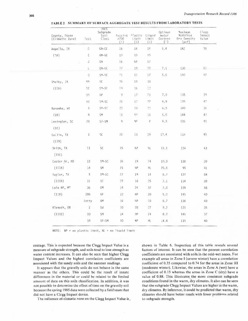
Bag samples of the surface aggregate and subgrade soil were collected at each test site for laboratory analysis. The soil from each site was tested to determine the grain size, liquid and plastic limit, optimum water content, maximum dry unit weight (ASTM DI557) , a nd Clegg Impact Value at the maximum dry unit weight. The data from these tests are summarized in Table 2 for the surface aggregates and Table 3 for the subgrade soils. It can be seen from these data that the surface aggregates are generally classified as gravels or sands with optimum water content below 10 percent. Maximum dry unit weights are in the 130 to 140 pcf (20.4 to 22.0 kN / m3) range and Clegg Impact Values are in the 40 to 50 range. The subgrade soils have a wid e r range of classifications, generally higher optimum water content, and lower maximum dry densities at optimum.
A good part of the laboratory testing was done to develop the relationship between the CBR and the Clegg Impact Value. The results of the laboratory CBR tests on nonsoaked subgrade soils are presented in Table 4. Each of the 21 subgrade soils was tested for three different moisture contents. The Clegg Impact Value is the average of the fourth readings obtained from the top and bottom of the molded sa mple.
STA TIS TI CAL RELATIONSHIPS
A simple linear regression analysis of the field data was performed in an attempt to develop functional relationships between test parameters . Of particular interest are the relationships of Clegg Impact Value versus moisture content and CBR versus Clegg Impact Value.
Clegg Impact Tests and Field Moisture Content
Several com bi nations of factors were used in the analysis of the data to isolate the effect of soil type and time of test. First, all soils and field test times were analyzed as one group. Then, various soil groups were considered separately and, finally. the data for a given soil group were analyzed by subdividing them into results from field tests in the summer of 1984 and spring of 1985. In this way, it was possible to determine the relationship for all soils and compare it to the relationship for a particular soil at a particular time .
The relationships between subgrade soil field water content and measured field Clegg Impact Value are given in Table 5. lt can be seen that all fine-grained soils and sands have a negative ,relationship between Clegg Impact Value and the water per-
308 Transportation Research Record I 106
TABLE 2 SUMMARY OF SURFACE AGGREGATE TEST RESULTS FROM LABORATORY TESTS
IJS S Sub()rade Optimum "aximum Clegg
County, State Soil Passing Plastic Liquid Water "1odified lmoact (Climatic Zone) Test Class F.200 L i111i t Limit Cont<>nt Dry Densitv Value
u (z;) (/;.) ( j ( cf
Wapello, IP. D r,~1-GC :6 14 12 5.4 142 38
(IA) E GM-GC 13 13 l'i
J SM l6 NP 17
L GM-GC ?7 l~ ~? 7. 1 130 61
f) SM-SC ?l 11 17 S.6 14[) 1\7
S~elby, IA qq SC ~fl l 'i 30
(I IA) SC S"-Sf. 11 ~6
SS GP 9 17 ~l i.0 135 3'1
vv S'-1-SC ?0 17 ~{ 6.9 135 4'.'
Kanawha, w SM-SC 2'? IB 'J') Ii .Q 140 3rc "
(IR) R GM 15 ~ID 15 5.B 144 4,,
Lexington, SC 20 SP-SM g ~F 8 fi. 3 136 45
(IC)
Coll in, TX GC ;>fl 13 29 l?. 1l llH 45
(I IR)
Smith, TX 11 SC 25 NP ~L 13. 1 134 43
( JIC)
Custer .NF, ND 13 S"l-SC 35 19 ?4 10.9 130 39
(!!IA) 14 SM ?l NP NL 25.6 95 41
Taylor, TX 5 S"l-SC 27 !<l 14 6.7 13? 54
(I I IB) 11 SC ~7 16 25 I. l 134 39
Lolo NF, MT 38 GM 14 24 32 3.8 139 48
(I IB) 208 GP 12 NP 20 5.0 145 40
Petty GM 16 ~p 20 6.7 136 40
Klamath, OR 2 SW 10 20 27 9.2 131 35
(I I IC) 10 SM 14 NP ?4 8.2 145 37
18 SP-SM 10 NP NL 14.4 115 40
NOTE: NP no plastic limit, NL =no liauid limit
centage. This is expected because the Clegg Impact Value is a measure of sub grade strength, and soils tend to lose strength as water content increases. It can also be seen that higher Clegg Impact Values and the highest correlation coefficients are associated with the sandy soils and the summer readings.
It appears that the gravelly soils do not behave in the same manner as the others. This could be the result of innate differences in the material or could be related to the limited amount of data on this soils classification. In addition, it was not possible to determine the effect of time on the gravelly soil because the spring 1985 data were collected by a field team that did not have a Clegg Impact device.
The influence of climatic zone on the Clegg Impact Value is,
shown in Table 6. Inspection of this tahle reveals several factors of interest. It can be seen that the poorest correlation coefficients are associated with soils in the cold-wet zones. For example all areas in Zone I (severe winter) have a correlation coefficient of 0.35 compared to 0.74 for the areas in Zone III (moderate winter). Likewise, the areas in Zone A (wet) ·have a coefficient of 0. 15 whereas the areas in Zone C (dry) have a value of 0.88. This illustrates the more consi tent ubgrade conditions found in the warm, dry climates . It also can be seen that the subgrade Clegg Impact Values are higher in the warm, dry climates. By inference, it could be predicted that warm, dry climates should have better roads with fewer pmblems related to subgrade strength.

ALKIRE 309
TABLE 3 SUMMARY OF SUBGRADE TEST RESULTS FROM LABORATORY TESTS
uses Sub~ra1e Optimum Maximum Clegg
County, State Soil Passing Plastic Liquid Water Modified Impact (Climatic Zone) Test Class #200 Limit Limit Content Dry Density Value
( ~-) ( ~ ) (%) (/;) (%)
Wapello, JA D CL 79 22 44 NA
(IA) GC 19 17 26
.J SM 36 26 32
L CL 78 '>? , __ 38 11. 7 113 39
Q "1L 82 27 38 14. 9 110 37
Shelby, IA RR CL 96 ?3 36
(!IA) l)D CL 90 23 40
SS SC 40 18 40 10.4 ll? 36
vv CL 93 25 45 13.0 112 39
Kanawha, WV 5 ML 57 23 30 11.0 127 27
(18) 8 SM-SC 22 13 19 6.4 130 36
Lexington, SC 20 SM 32 NP 15 9.2 128 37
(IC)
Coll in, TX CL 60 ;>Z 44 17 109 36
(I IR)
Smith, TX 11 SM 25 NP NL 10.4 125 30
(I IC)
Custer NF, ND 13 CL 54 19 34 10.4 115 35
(I I IA) 14 ML 71 NP ?.4 13.0 118 23
Taylor, TX 5 CL 77 19 29 11.1 121 40
(I I IB) 11 SC 38 22 34 9. 9 124 27
Lolo NF, MT 38 G"1-GC 25 19 25 6.7 133 44
(I IR) 208 GM 21 23 25 6. 5 128 34
Petty GM ?.O NP 30 6. 9 132 39
Klamath, OR ? SM 19 2 39 17 107 32 ' (I I IC) 10 ML NA NA NA 16 107 33
18 SW-SM 10 NP NL 3D 75 35
NOTE: 'IP no plastic limit, NL = no liquid limit, NA = not available
California Bearing Ratio and Clegg Impact Value
The 62 data points that represent the CBR and Clegg Impact Values obtained from laboratory tests (Table 4) were also analyzed by use of regression equations. The results from this analysis are tabulated as follows :
Equation Number
I 2
Equation
logCBR = -0.649 + 1.671 ogC/V CBR = 3.35 + 0.0803CIV2
Correlation Coefficient
0.94 0.88
Based on the correlation coefficient va lues, the best fit is the foll owing log-log equation:
logCBR = -0.649 + l.671ogC/V (1)
or its equivalent
CBR = 0.2244C/Vl.67 (2)
which is comparable to the equation proposed by Clegg (2)
CBR = 0.07CJV2 (3)

TABLE 4 NONSOAKED CALIFORNIA BEARING RATIO LABORATORY TEST RESULTS FOR SLIBGRADE SOILS
Moisture Dry California Clegg
County, State Test Content Density Bearing Impact
( %) (pcf) Ratio Value
Klamath, OR 2 11.1 103.0 103 38
18.4 102.6 3
18.8 102.0 2
10 15.6 105.4 142 36
17.7 105.3 26 18
20.7 100.D 3 6
18 23.1 78.9 88 27
24.5 79.8 36 18
28.0 77 .6 8 11
29.8 77 .3 2
34.0 72.4
Lo lo NFa, MT 38 3.8 126.1 113 25
8.0 129.7 41 22
10.0 125.7 3 8
208 2. 1 122.9 144 28
5.6 125.6 129 32
9.5 122.2 11 10
Petty 3.2 122.8 74 27
4.5 127.5 84 30
8.8 128.7 7 13
9.4 127.2 3 8
9.7 126.8 3
Custer NFa, ND 13 7.6 109.1 58 28
9.8 113.8 36 23
22.9 97.6 3 4
14 10.0 114.2 34 23
12.8 112.2 11 12
16.8 107.3 2
Collin, TX 7.2 101. 4 38 NA
17. 104.4 29 NA
22.2 100.8 10 NA
Fannin, TX 9 7.9 115.6 88 36
11.3 118.0 26 20
15.5 109.6 2 4
Smith, TX 11 7.9 115.2 66 28
11.3 121.6 17 12
14.0 115. 9 3 4

TABLE 4 continued
Moisture Dry California Clegg
County, State Test Content Density Bearing Impact
( 'I: ) ( pcf) Ratio Value
Smith, TX 11 4.7 107.6 17 13
11.1 109.6 2 10
14 .1 102.2 2
Taylor, TX 5 8.3 116. 7 78 34
11. 2 121.4 45 27
15.5 114.8 5
11 7.0 120.3 71 36
10.4 121. 7 25 NA
13.5 116. 1 3 5
Kanawha, :VV 5 5.7 116 .6 66 N~.
10. 1 120.2 41 NA
14. 3 118. 6 NA
8 6.9 125.6 96 NA
8. 4 129.0 38 23
11. 1 122.2 3
Lexington, SC 14 6.4 111. 6 81 33
13. 1 116.0 20 14
17.6 109.5 2 3
17 3.1? 116. 1 27 13
7.5 119 .6 28 12
7 .8 118.4 20 11
12.7 115 .6 3 4
20 3.7 113.7 33 15
9.4 104.8 48 22
14 .3 90.5 2
Houghton, ~I Massie 3.4 132. 4 78 36
6.5 142.7 107 34
7.3 141. 9 91 ?8
9.;' 138.2 12 12
Mass it: 5.6 114. 7 37 '!C LO
7 .0 119. 9 56 27
9,5 124.4 63 34
l?.4 115.2 6 11
a NF = Nation2l Forest
NOTE: NA = not availablr
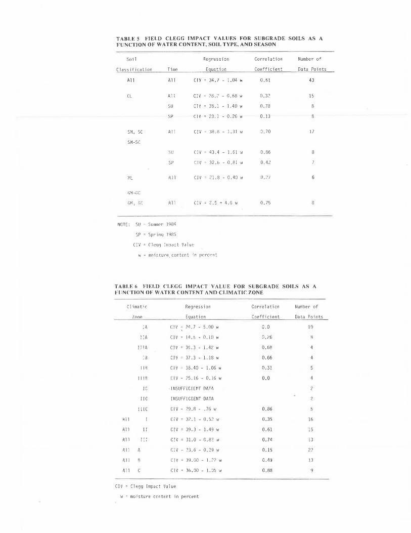
TABLES FIELD CL EG G IMPACT VALUES FOR SUBGRADE SOILS AS A FUNCTION OF WATER CONTENT, SOIL TYPE, AND SEASON
Soi 1 Regression Correlation Number of
Classification Time Equation Coefficient Data Points
A 11 All CIV 34.7 - l. 04 w 0.61 43
CL A 11 CIV 28.~ - 0.68 w 0.32 15
SU CIV 38.1 1.40 w 0.78 8
SP CIV 23.1 0.26 w 0.13 8
SM, SC A 11 CIV 38. 8 - 1. 31 w 0. 70 17
SM-SC
SU CIV 43.4 1.61 w 0.86 8
SP crv 32.G 0.81 w 0.4~
:>ll All CIV 21.8 - 0. 40 w 0.27 6
GM-GC
GM, GC A 11 CIV Z.5 + 4.6 w 0. 75 8
NOTE: SU Su1nmer 1984
SP Spring 1985
CIV Clegg Impact Value
w = m0isture.content in percent
TABLE 6 FIELD CLEGG IMl'ACT VALUE FOR SUBGRADE SOILS AS A n :NCTION 01' WAH:R CONTENT AND CLIMATIC ZONE
Climatic Regression Correlation Number of
Zone Equation Coefficient Data P0ints
IA crv 24.7 5.00 w 0.0 10
I IA CIV 14.6 0.10 w 0.26 8
I I TA CIV 36.3 1.42 w 0.G8 4
IB CIV = 37. 3 - 1.18 w 0.66 4
I IR CTV = 38.40 - 1.06 w 0.31
I I 1 g CIV = ?5 .16 - 0.16 w 0.0
IC INSUFFICIENT OATA
I IC INSUFFICIENT DATA ?
! I IC CTV 29.8 .7fi w 0.86
.~ 11 cTv 32. 1 0.52 w 0.35 16
A 11 IT CIV 39.3 1.49 w 0.61 15
All JI I CIV = 31.0 - 0.82 w 0. 74 13
All A CIV 23.6 - 0.29 w 0.15 22
A 11 CTV 39.00 - 1.22 w 0.49 13
All c CIV = 36.00 - 1.05 w 0.88 9
C!V = Clegg Impact Value
w = moisture content in p~rcent
ALKIRE
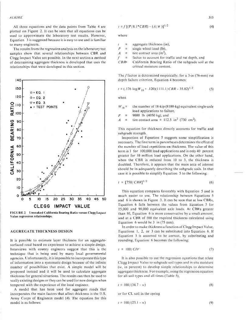
All three equations and the data points from Table 4 are plotted on Figure 2. It can be seen that all equations can be used to approximate the laboratory test results. However, Equation 3 is suggested because it is easy to use and is familiar to many engineers.
The results from the regression analysis on the laboratory test samples show that several relationships between CBR and Clegg Impact Value are possible. In the next section a method of determining aggregate thickness is developed that uses the relationships that were developed in this section.
140
130 • El = EQ. I
120 0 = EQ. 2
0110 'V = EQ. 3 •
t- • = TEST POINTS
~ 100
(!) 90 • • z . ' a: 80 ct
"" 70 m •
ct 60
z 50 a:
0 l&.. 40 _J
ct 0
10
0 0 5 10 15 20 25 30 35 40 45 50
CLEGG IMPACT VALUE F IG UR E 2 Unsoaked California Bearing Ratio versus Clegg Impact Value regression relationships.
AGGREGATE THICKNESS DESIGN
It is possible to estimate layer thickness for an aggregatesurfaced road based on experience to achieve a simple design. Interviews with county engineers suggest that this is the technique that is being used by many local governmental agencies. Unfortunately, it is impossible to incorporate this type of information into a systematic design because of the infinite number of possibilities that exist. A simple model will be proposed instead and it will be used to calculate aggregate thickness for general situations. The results can then be used to verify existing designs or they can be used for new designs when tempered with the experience of the local engineer.
A model that has been used for aggregate roads that incorporates the main factors that affect thickness is the U.S. Army Corps of Engineers model (4) . The equation for this model is as follows:
t =f[(P / 8. l*CBR) - (A / rr )]1 / 2
where
aggregate thickness (in), single wheel load (lb), tire contact area (in2),
313
(4)
I = p = A = f = CBR=
factor to account for traffic and rut depth, and California Bearing Ratio of the subgrade soil at the critical moisture content.
The f factor is determined empirically; for a 3-in (76-mm) rut depth failure criterion, Equation 4 becomes:
I= (.176 logW 18 + .120)(1111.1/CBR-35.82) 112 (5)
when
W18 = the number of 18-kip (8100-kg) equivalent single-axle load applications to failure,
P = 9000 lb (4050 kg), and A = tire contact area = 112.5 in 2 (730 cm 2) .
This equation for thickness directly accounts for traffic and subgrade strength.
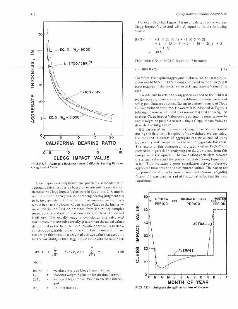
Inspection of Equation 5 suggests some simplification is necessary. The first term in parentheses determines the effect of the number of load repetitions on thickness. The value of this term is I for .100,000 load applications and is only 40 percent greater for 10 million load applications. On the other hand, when the CBR is reduced from 10 to 3, the thickness is doubled. Therefore, it appears that the main area of in"terest should be in adequately describing the subgrade soils. In that case it is possible to simplify Equation 5 to the following:
t = [750 / CBR] 112 (6)
This equation compares favorably with Equation 5 and is much easier to use. The relationship between Equations 5 and 6 is shown in Figure 3. It can be seen that at low CBRs, Equation 6 falls between the values from Equation 5 for 15,000 and 90,000 equivalent axle loads. At CBRs greater than 10, Equation 6 is more conservative by a small amount, and at a CBR of 100 the required thickness calculated using Equation 6 would be 3 in (75 mm) .
In order to make thickness a function of Clegg Impact Value, Equations l, 2, or 3 can be substituted into Equation 6. If Equation 3 is assumed to be correct, by substituting and rounding, Equation 6 becomes the following:
I = 100/ CIV (7)
It is also possible to use the regression equations that relate Clegg Impact Value to subgrade soil types and in situ moisture (w, in percent) to develop simple relationships to determine aggregate thickness. For example, using the regression equation for all soil types and all times (Table 5),
I= 100 / (34.7 - w) (8)
or for CL soil in the spring
I= 100/(23.1 - w) (9)
314
30
z 25
en en LLJ z ~ (.)
~ 1--
20
!5
10
5
I \
t= ( 750/ CBR )112
t=IOO/CIV
0 o 5 10 15 20
RATIO CALIFORNIA BEARING
0 5 10 15 18
CLEGG IMPACT VALUE Fl(;L; RE 3 Aggregate thickness versus California Bearing Ratio or Clegg linpact Value.
These equations emphasize the problems associated with aggregate thickness design based on in situ soil characteristics.
Because the Clegg Impact Value. or 11· in Equations 7. 8. and 9. is not a constant for a given soil some engineeringjudgment has
to be incorporated into the design. The conservative approach would be to use the lowest Clegg Impact Value or the highest 11·
measured in the field or obtained from laboratory samples
prepared at standard critical conditions, such as the soaked
CBR test. This usually leads to over-design and calculated
thicknesses that are substantially greater than the actual values determined in the field. A more realistic approach is to use a
concept comparable to that of accumulated damage and base
the design thickness on a weighted average value that accounts
for the variability of the Clegg Impact Value with the season (5).
WCIV
where
WCIV F
I
CIV;
Al;
=
:;
n
F;CIV;AI;/ if.I Al; (10)
weighted average Clegg Impact Value,
seasonal weighting factor for ith time interval, average Clegg Impact Value in ith time interval,
and ith time interval.
Transportation Research Record I 106
For example, when Figure 4 is used to determine the average Clegg Impact Value and with F; equal to I, the following
results:
WCIV = ((I X 20 X I) + (I X 5 X 2) + (I X 15 X 7) + (I X 50 X 2)) / (I + 2
+ 7 + 2)
= 19.6
Then, with CIV = WCIV, Equation 7 becomes
t = 100/ WCIV ( 11)
Therefore, the required aggregate thickness for the example just
given would be 5.1 in ( 129.5 mm) compared to the 20 in (508.0
mm) required if 1he lowes1 value of Clegg impac1 Value (5) is
used. It is difficult to relate this suggested method to the field test
results because there are so many different climatic zones and
soil types. Data are also insufficient to define the curve of Clegg Impact Value versus time. However, it is indicated in Figure 4
(obtained from actual field measurements) that the weighted
average Clegg Impact Value occurs during the summer months
and it might be possible to use a single Clegg Impact Value to
describe the subgrade soil. If it is assumed that the summer Clegg Impact Value obtained
during the field visits is typical of the weighted average value, the required thickness of aggregate can be calculated using
Equation 8 and compared to the actual aggregate thickness.
The results of this comparison are tabulated in Table 7 and plotted in Figure 5. In analyzing the data obtained from this
comparison, the square of the correlation coefficient between
the actual values and the points calculated using Equation 8 is 0.4. This indicates a poor correlation between observed
aggregate thickness and the calculated values. The reason for
the poor correlation is because an incorrect seasonal weighting
factor of I was used instead of the actual value that fits local
conditions.
60
LLJ ::> 50 ...J
~ 1--(.) <( a.. ::E
(!) (!) LLJ ...J (.) 10
SPRING SUMMER - FALL
PERIOD PERIOD
AVERAGE r_L _________ I I I I
M A M J J A S 0 N
MONTH OF YEAR FIG URE 4 Subgrade strength versus time of the year.
WINTER
PERIOD
D J F

TABLE 7 CALCULATED SEASONAL WEIGHTING FACTORS FOR DIFFERENT CLIMATIC ZONES
Location Test Subgrade CIVsu Ac tu a 1 Calculatea Calculatedb
(Climatic Zone) Soil Aggregate Aggregate F. l
Classifi cation Thickness Thickness
in. in.)
Wapello, IA D CL 10 3.5 . 10.0 2.9
(IA) E GC 26 2.0 3.8 1. 9
J SM 27 2.0 3.7 1. 9
L CL 14 4.0 7 .1 1.8
Q SC 27 1. 3 3.7 2.8
Zone Average 21 2.6 5.7 2.3
Shelby, IA DD CL 18 2.5 5.6 2.2
( IIA) SS SC 13 0.5 7.7 15.4
vv CL 10 5.3 10.0 1. 9
RR CL 19 Ll 5.3 1. 5
Zone Average 15 3.6 7.2 1. 9
Custer NF, NO 13 CL 12 6.0 8. 3 1.4
( IIIA) 14 ML 24 3.0 4.2 1.4
Zone Average '0 1U 4.5 6.2 l.4
Kar;awhn, WV 5 ML 19 5.0 5.3 l. l
( IB) 8 Sr-!- SC 38 8.0 2.6 0.3
Zone Average 29 6.5 4.0 0. 7
Collins, TX CL 11 7.0 9 .1 1. 3
(I IB)
Taylor, TX LL 22 6.0 4.5 0.8
(l I rn) 11 SC 24 6.0 u 0.7
Zone Average 23 6.0 4.7 .8
Le xington, SC SM 36 7. .0 2. 8 1.4
(IC)
Smith, TX 11 SM 30 8.0 3.3 0.4
(I IC)
Klamath, OR 2 SM 26 8.0 3.8 0.5
(I I IC) 10 ML 10( P . 5 10.0 0.8
18 SW-SM 19 6.0 5.3 0.9
Zone AvPra ge 18 8 .8 G.4 . 1
~ f 100 h 100 C!Vsu
F. nr · "ca le , tactual SU

Ji6
z .. 12
Cf) Cf) UJ z ~ 10 (.)
:c ......
UJ 8 ...... 0 C( (.!) UJ D::
6 (.!) (.!) ~
0 UJ 4 .... C( ...J ::> (.) 2 ...J C( (.)
0 0
ACTUAL
•=CLIMATIC ZONE AVERAGE O• ACTUAL
0 0
• 0
•o
• ~
0 0 0
0 ~ • 8 0 0
• • 0
2 4 6 8
AGGREGATE THICKNESS, IN.
Transportation Research Record 1106
To determine the average seasonal weighting factor for the different climatic zones, the observed aggregate thickness and the summer Clegg Impact Value were substituted into Equation 8, and an average seasonal weighting factor, F;, was backcalculated. The results of this calculation are also shown in Table 7. It is shown in Table 7 that the cold climatic regions have high values for the seasonal weighting factor. It can also be seen that there is a fair variation of values within any climatic zone.
A matrix of average values for the seasonal weighting factor and calculated and observed aggregate thickness for each climatic zone is shown in Table 8. It can be seen that the roads in warm, dry climatic zones generally use more aggregate. The least amount of aggregate is associated with the data collected at Lexington County, South Carolina, in climatic zone IC.
FIGURE 5 Calculated versus actual aggregate thickness.
The averages of ail values are also shown in Table 8. it can be seen that the average observed thickness is 5.4 in (137.2 mm) compared to 5.3 in ( 134.6 mm) for the calculated thickness. An improvement in the relationship between calculated and observed thickness can therefore be made if the average Clegg Impact Value for each climatic zone is used to determine the resulting thickness. These values are shown by the darkened symbols plotted on Figure 5. In this case, the relation between the calculated and observed aggregate thickness is higher with a correlation coefficient of 0.7. Therefore, Equation 8 is adequate for most calculations to determine aggregate thickness, if enough data can be collected to allow the local engineer to determine the average seasonal weighting factor.
TABLE 8 AVERAGE SEASONAL WEIGHTING FACTOR MA TRIX
Climatic Zone Seasonal Actual Calculated
Weighting Aggregate Aggregate
Factor Thickness Thickness
(in.) (in.
IA 2.3 2.6 5.7
IB 0. 7 6.5 4.0
IC l. 4 2.0 2.B
Zone Average l. 5 3.7 4.2
!IA l. 9 3.6 7.2
l l~ l. 3 7.0 9. l
!IC 0.4 B.0 3.3
Zone Average l. 2 6.2 6.5
!!IA l. 4 4. 5 6.2
I I IB O.B 6.0 4.3
I I IC 0.7 B.B 6.4
Zone Average l. 0 6.4 5.2
Average of all l. 2 5.4 5.4

ALKIRE
The one item of interest to the engineer that has not been mentioned is how the roads performed in relation to their thickness. During each of the site visits, the project personnel made a subjective evaluation oft he condition of all sections that were tested. At the time of the field visits, all of the test sites were in good condition. There were no restrictions on driving speed or comfort and no indications of subgrade failures . The only observed performance problem was at a site in Iowa at which the roads were slippery when wet. However, this is more likely related to the aggregate gradation rather than an insufficient aggregate thickness.
The fact that the roads were in good condition might indicate that the roads were adequately designed for the level of traffic that they were carrying. It might also indicate that the roads were over-designed and aggregate was being wasted. It is impossible to determine which case is correct. However, the fact that the cold, wet climatic zones have less aggregate, and still have passable roads, suggests that many of the aggregate roads that are currently being constructed are somewhat overdesigned.
SUMMARY
A simple aggregate thickness design procedure was suggested. The design was based on the Corps of Engineers equations for low-volume roads and requires an indication of the subgrade strength in terms of the subgrade Clegg Impact Value.
Subgrade strength was determined in this paper by use of the Clegg Impact device and the relationships between CBR and Clegg Impact Value were developed from laboratory tests on collected field samples. It was shown that Clegg's relationship that related Clegg Impact Value to CBR was suitable to describe the soil for the sites tested.
Field results were used to show that the thickness design equations could be simplified to an inverse function of a
317
weighted Clegg Impact Value (Equation 8) that incorporated climatic conditions into the design equation through a seasonal weighting factor.
The suggested design procedure can be made site-specific if one collects enough data to accurately define the weighted Clegg Impact Value for particular climatic conditions. This value can then be used to determine the aggregate thickness based on particular local conditions instead of the data collected in this research.
ACKNOWLEDGMENTS
The work presented in this paper was developed as part of a project sponsored by the Federal Highway Administration entitled "Design and Operation of Aggregate-Surfaced Roads." Their support is gratefully acknowledged. Laboratory tests were performed by Jerome Breyer.
REFERENCES
I. S. H. Carpenter, M. I. Darter. and B. J. Dempsey. Evaluation of Pavement Systems for Moisture-Accelerated Distress. In 7i·an.1por-1a1ion Research Record 705. TR B. National Research Council, Washington, D.C., 1979.
2. B. Clegg. An Impact Soil Test for Low Cost Roads. Proc .. 2nd Road Enl(ineerinl( Associat ion of Asia and Australia, Manila, Philippines, 1978.
3 . B. Clegg. Application of an Impact Test to Field Evaluation of Marginal Base Course Material. In Tramportation R<'.vearch Record 898, TRB, National Research Council. Washington, D.C., 1983 .
4. Thicknes.1· Requirement /(Jr Umurfaced Road.1 and Air/i'elds. TRS 70-5. U.S. Army Co rps of Engineers, Waterway Experimental Station, Vicksburg, Mississippi, 1970.
5. Swfacing Handhook . FSH 7709 .569. U.S. Forest Service, U.S. Department of Agriculture, Washingto n, D.C., 1983.