An Aerodynamic Optimization Method Based on the …aiollo/Papers_files/Journal of... · An Aerodynamic Optimization Method Based on the Inverse Problem ... at the wall is optimized

Journal of Computational Physics 173, 87–115 (2001)doi:10.1006/jcph.2001.6845, available online at http://www.idealibrary.com on

A n A e r o d y n a m ic O pti m iz a ti o n M e th o d B a s e do n th e In v e rs e Pr o b l e m A d j o i nt E q u a ti o n s

A. Iollo, M. Ferlauto, and L. Zannetti

Dipartimento di Ingegneria Aeronautica e Spaziale Politecnico di Torino, C.so Duca degliAbruzzi 24, 10129 Torino, Italy

E-mail: [email protected], [email protected], [email protected]

Received April 5, 2000; revised May 23, 2001

An adjoint optimization method, based on the solution of an inverse flow prob-lem, is proposed. Given a certain performance functional, it is necessary to findits extremum with respect to a flow variable distribution on the domain boundary,for example, pressure. The adjoint formulation delivers the functional gradient withrespect to such a flow variable distribution, and a descent method can be used foroptimization. The flow constraints are easily imposed in the parameterization of thedistributed control, and therefore those problemswith several strict constraints on theflow solution can be solved very efficiently. Conversely, the geometric constraintsare imposed either by additional partial differential equations, or by penalization.By adequately constraining the geometric solution, the classical limitations of theinverse problem design can be overcome. Several examples pertaining to internalflows are given. c! 2001 Academic Press

Key Words: adjoint method; inverse problem; optimization; compressible flow.

1. INTRODUCTION

Aerodynamic design can be assisted in two essentially different ways. One, the classicapproach, is based on the inverse problem solution; the other, which is more recent, relieson numerical optimization.In the inverse problem onemust usually determine unknowns that are given in the natural,

i.e., direct position of the problem. For example, a typical inverse problem is to find the airfoilgeometry, given the flight speed and the pressure distribution on its surface. In the clas-sical works of Mangler [1] and Lighthill [2] the airfoil inverse problem was solved inthe framework of potential flows and with the use of conformal mapping. Further de-velopments of this solution method are extensively accounted in [3] and are related tothe introduction of viscous models for laminar and turbulent flows and to the solvabil-ity conditions of the problem. Other examples of inverse problem solution methods are

87

0021-9991/01 $35.00Copyright c! 2001 by Academic Press

All rights of reproduction in any form reserved.

88 IOLLO, FERLAUTO, AND ZANNETTI

found in the collection AGARD-R-780. In addition, Polito’s [4] approach, relative tothe spectral solution of the inverse problem for airfoils, and that of Bauer et al. [5] forshockless airfoils, should be mentioned. One drawback of inverse problems is that theymay be ill posed, as certain wall pressure distributions on airfoils result in open or self-intersecting profiles. Lighthill [2] discovered the solvability conditions that should be re-spected by pressure distributions within an incompressible potential flow model, whereasthe solvability conditions for compressible flows were investigated in [6] and referencestherein.The appeal of the inverse problem solution for aerodynamic design declined as powerful

computers and sound numerical methods that allow numerical optimization of aerodynamiccomponents became available. Once a functional that defines the relative merit or costof a certain solution is defined, a numerical optimization algorithm can be as simple as(i) computing the functional gradient relative to the controls by divided differences, (ii)marching toward the functional extremum using gradient information. If the number ofparameters that have to be optimized is in fact not very small, finding the gradient requires ahuge amount of computational time. The computation of each gradient component needs aflow evaluation, making optimizations using the Euler or Navier–Stokes models unfeasible.Greater computational efficiency is obtained by using the adjoint method (see [7–9]) to

compute the functional gradient. Evaluation of the gradient requires one adjoint calculationand one flow calculation, regardless of the number of design variables. This approach hasopened up the possibility of optimizing tridimensional compressible viscous flows overwing–body configurations at high Reynolds numbers; see [10].The advantages of numerical optimization over the inverse problem can be summarized

in that numerical optimization allows themaximization or minimization of global quantitiessuch as lift or drag in the presence of constraints, whereas for inverse problems the designis limited to the pressure distribution selection on the boundary, which is given on the basisof designer experience and is therefore somewhat arbitrary. In addition, no control of thefinal geometry is possible. In this work we try to overcome these weaknesses by extendingthe adjoint optimization method to inverse problems.To formulate a shape optimization problemwe need a functionalF to be eitherminimized

or maximized. We have F = F[U (!),!] where U is the flow variables vector and !represents the geometry. In the adjoint method such an extremum problem is solved usinga variational technique and introducing a Lagrange multiplier vector " dual of the flowvariables vector. Using the Lagrange multipliers we are able to write #F for !" ! + #!,at the cost of solving a system of partial differential equations (PDEs) for the Lagrangemultipliers which is the mathematical adjoint of the governing equations. Once the gradientis known, the initial geometry is perturbed accordingly and the procedure is started all overagain until a convergence criterion is satisfied.The adjoint method can be adapted to an inverse problem formulation. Let p(s) be

the flow quantity we prescribe on the flow-field boundary, where for example p is thepressure and s is the curvilinear coordinate along the boundary. We define a cost/meritfunctional in much the same way as before: F = F[U (p), p]. It should be noted thatthe control is now the pressure distribution on the boundary, whereas in usual adjointmethods the control is the boundary shape. The derivation of the adjoint follows the samesteps as in the shape optimization case, to finally obtain #F for p(s)" p(s) + #p(s).The pressure distribution is then altered according to the gradient information until theextremum is eventually reached. In this formulation the boundary shape results from the

AERODYNAMIC INVERSE PROBLEM ADJOINT EQUATIONS 89

solution of the inverse problem corresponding to each optimization step. In this respect theoptimization of an inverse problem can be considered a flow design optimization as opposedto the optimization of a direct problem, which is known as shape design optimization. Theidea of optimizing the pressure distribution is not new; it was proposed in [11] with themotivation that “this procedure avoids most if not all of the limitations of the pure inversemethod.”Flow design optimization offers a very simple way of implementing flow constraints,

as they can be directly included in the parameterization of the control. Inevitably, inthe design process it is necessary to focus on a given model to account for the physi-cally relevant phenomena which affect performance. Yet, it is mandatory to include re-sults obtained by more sophisticated models or other disciplines, in the selected model.These results usually take the form of constraints on the governing equation variables,and not on the geometry. For example, let us consider a propeller to be designed to max-imize traction for given shaft work. The selected model is that of an inviscid compress-ible fluid governed by the compressible Euler equations, a model that is appropriate tocompute the traction of a propeller. However, one must also take into account the con-straints on the emitted noise. These requirements may have the form of constraints onthe load of the propeller blades, which in turn is a function of the flow variables at thewall. Therefore any time we have a design problem where the effects that are not rep-resented in the governing equations are to be considered, the optimization based on thesolution of the inverse problem adjoint equations is a natural way of formulating theproblem.For example, in the numerical tests, a diffuser is studied where the pressure distribution

at the wall is optimized for minimal axial deviation at the outlet. The maximum attainablepressure gradient is constrained in order to avoid premature flow detachment. In the usualadjoint optimal shape design formulation, flow constraints are accounted for either throughadditional Lagrange multipliers, which means there are additional PDEs to be solved, orby a penalization in the functional. For the method proposed here, the situation is reversed:Geometric constraints result in either additional PDEs or in functional penalization. Hence,for example, the inverse problem closure and univalence conditions for airfoils are bypassedby imposing appropriate geometric constraints on the solution.In the following, the problem is formulated and the gradient is derived in detail for two

applications which are solved using an inverse problem. The first example is intended tomake the ideas clear. We then concentrate on a case that is complicated by a flow modelwhich describes a turbo fan stage. As previously mentioned, the first case concerns theproblem of designing a diffuser. We wish to determine the wall pressure distribution so thatthe flow axial deviation at the outlet is at a minimum, with constraints on the allowed wallpressure gradient.The second example is more oriented to applications and is related to a flow model

of a complete piece of turbo-machinery; see [13]. The blades of the turbo-machinery aremodeled as flow surfaces of zero thickness which exert forces on the fluid flow. Thisapproximation introduces volume forces in the compressible Euler equations, which isthe model adopted for the flow. Our method is such that, instead of modifying the shapeof the flow surfaces that model the blades, we give the force that the blades exert on theflow and let the geometry accommodate this distribution of forces. The volume force dis-tribution itself is modified according to the functional gradient, so that, for example, thrustis maximized.


2. DIFFUSERWITH MINIMAL AXIAL DEVIATION AT THE OUTLET

Let us consider a two-dimensional diffuser with total pressure, total temperature, andflow angles imposed at the inlet; pressure is given at the outlet. The walls of the diffusershould be designed so that the flow at the outlet has minimal axial deviation and the diffusercauses a given pressure rise with a constraint on the maximum wall pressure gradient.The constraint imposed qualitatively reflects the Stratford [14] semiempirical separationcriterion for decelerated turbulent boundary layers,

cp

!sdcpds

= Cs110 , (1)

where C is a constant function of the Reynolds number per unit length, s is the wall curvi-linear coordinate, and cp is the pressure coefficient. We take s # x and cp = 2 p$ pin

$U 2in, where

in refers to the inlet section.As the dynamic pressure is approximately equal to the differencebetween the total pressure p0 and the inlet pressure pin, we obtain dp

dx #dcpdx (p0 $ pin). The

maximum allowable pressure gradient at the wall II(x) is displayed in Fig. 1. In addition,the gradient is also required to be positive. This simple problem can be encountered in thedesign of wind tunnel diffusers, air-breathing engine intakes, or turbo-machine casings.

2.1. Flow Model and Inverse Problem Solution Method

The flow is governed by the two-dimensional compressible Euler equations. In Cartesiancoordinates (x, y), one has

%U%t

+ %F%x

+ %G%y

= 0, (2)

FIG. 1. Constraint on the pressure gradient along the x-axis.


where

U =

"##$

##%

$

$u$w

e

&##'

##(F =

"###$

###%

$up + $u2

$uwu(p + e)

&###'

###(G =

"###$

###%

$w

$uwp + $w2

w(p + e)

&###'

###(,

and as usual, $ is the density, p is the pressure, and e is the total internal energy per unitvolume. The diffuser geometry is unknown, but it is obtained by imposing a given pressuredistribution p = pe(s) on the solid boundaries, as opposed to direct problems where thegeometry is known and the no-through-flow condition applies on the diffuser walls. In thissense, for the sake of conciseness, we can write Eq. 2 as E(U, pe) = 0.This solution method is based on the ideas presented in [15] and [16]. The diffuser

walls can be considered deformable and impermeable surfaces fastened to the diffuser inletsection that move under the effect of the imposed pressure. An initial wall configuration isguessed. The resulting transient is described by integrating the equations that govern thetime-dependent flow motion. The results differ from those of a usual flow solver in twoways. The first is that the no-through-flow boundary condition at the wall is replaced bya condition of given pressure; the second is that the number of equations that must solvedis increased by one, the kinematic equation governing the surface motion. This equation isobtained by imposing the condition that the speed of the moving wall must be locally equalto the normal flow velocity. Therefore, in terms of computational cost, the inverse problemsolution is equivalent to a direct solution.A finite volume formulation, based on the approximate Riemann solver [17] to compute

the fluxes at cell interfaces, is applied. Second-order spatial accuracy is obtained using anENO class method [18]. At the end of the transient, the walls assume the shape that solvesthe inverse problem, i.e., find the shape which induces the given pressure distribution onthe walls.

2.2. Variational Formulation, Adjoint Equations, and Gradient

The wall pressure pe(s) that should be imposed on the diffuser walls which minimizethe functional

D[pe(s)] = 12

)

out

*w

u

+2dy (3)

has to be determined. In order to solve such a constrained extremum problem, we introducethe Lagrangian function

L(U, pe,") = D +)

&

t"E(U,pe) d&, (4)

where t"(x, y) = {'1, '2, '3, '4} are Lagrangemultipliers. This approach allows us to treatthe problem as unconstrained. A stationary configuration is found when the variation of Lwith respect to all its arguments, which are now considered independent functions, is 0.Computing #L as in [20], we obtain

#L = #LU + #Lpe + #L" (5)


with

#LU = #DU +)

(

t"(FUnx +GUny)#U d) $)

&

(t"xFU + t"yGU )#U d&, (6)

where( is the boundary of flow field&, and FU ,GU are the Jacobian matrices of F andG.All contributions to #L must be 0 at the maximum. Hence, to find a stationary point, we

enforce

#LU = 0 #L" = 0.

In general this results in #Lpe %= 0. To reach the minimum, we take #pe so that #L =#Lpe < 0. It should be noted that the variations ofLwith respect to the Lagrangemultipliers" simply yield the flow equations.From the condition #LU = 0, the adjoint of the Euler equations and its boundary condi-

tions are obtained.

t"xFU + t"yGU = 0 in & (7)

and,w

u%

%U

*w

u

+h(() + t"(FUnx +GUny)

-#U = 0 on (, (8)

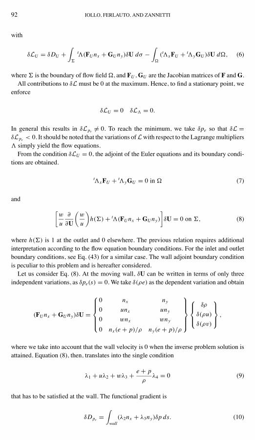
where h(() is 1 at the outlet and 0 elsewhere. The previous relation requires additionalinterpretation according to the flow equation boundary conditions. For the inlet and outletboundary conditions, see Eq. (43) for a similar case. The wall adjoint boundary conditionis peculiar to this problem and is hereafter considered.Let us consider Eq. (8). At the moving wall, #U can be written in terms of only three

independent variations, as #pe(s) = 0. We take #($e) as the dependent variation and obtain

(FUnx +GUny)#U =

"###$

###%

0 nx ny0 unx uny0 wnx wny0 nx (e + p)/$ ny(e + p)/$

&###'

###(

"#$

#%

#$

#($u)#($v)

&#'

#(,

where we take into account that the wall velocity is 0 when the inverse problem solution isattained. Equation (8), then, translates into the single condition

'1 + u'2 + w'3 + e + p$

'4 = 0 (9)

that has to be satisfied at the wall. The functional gradient is

#Dpe =)

wall('2nx + '3ny)#p ds. (10)


2.2.1. Pressure Parameterization

The diffuser has imposed inlet pin and outlet pout wall pressures. The distributed controlis the wall pressure gradient. On the discrete level, the pressure is recovered as

pe(xi ) = pin +i.

j=2m(x j )*x j , m(x j ) =

*dpedx

+

j(11)

with the constraint

N.

j=2m(x j )*x j = pout $ pin (12)

to match the exit pressure. *x j is the grid size in the x-direction and N is the number ofcomputational points in the x-direction. We have N $ 1 control parameters represented bythe pressure gradient at the discretization points.Let us consider Eq. (10) and discretize it as

#Dpe =N.

j=2+ j#p j , (13)

with + j = [('2nx + '3ny)*s] j and #p j =/ j

i=2 #m(xi )*xi . We have

#Dpe =N.

i=2#m(xi )*xi

N.

j=i+ j . (14)

Take ,i = *xi/N

j=i + j . If there were no constraints on the pressure gradient, wecould simply set #m(xi ) = $-,i to obtain #D < 0. Yet, in view of Eq. (12), we alsoobtain

N.

i=2.i#m(xi )*xi = 0. (15)

If 0 & m(xi ) & /(xi ), then .i = 1; otherwise we take #m(xi ) = 0 and .i = 0. By project-ing the gradient onto the plane tangent to the constraints (see Fig. 2) we have #D < 0 bytaking

{0i }' {,i }' {0i } = #m(xi ) = -

0

1,iN.

j=2.2j $ .i

N.

j=2, j. j

2

3. (16)

The solution of the optimization problem is achieved by initializing the coefficients m(x j ),computing the corresponding wall geometry using the inverse problem, solving the adjointequations, and updating the coefficients m(x j ), according to the projected gradient, untilthe minimum is reached.


FIG. 2. Projection of the gradient onto the constraint space.

2.3. Comparison with Classical Adjoint Formulation

The same problem can be solved by an adjoint formulation where the controls are theposition of the upper boundary discretization points. In such a case, the functional to beminimized is

D1[!w] = 12

)

out

*w

u

+2dy, (17)

where!w is the upperwall. The solution to such a problemwould be a straight duct, however,leading to the same pressure at the inlet and outlet. In order to accomplish a certain pressureincrease between the inlet and outlet it is also necessary to require that

D2[!w] =4pwin $ p(in

52 =)

!w

[pw(!w)$ p(in]2 f (!w) d!w

be minimized, where pwin is the actual wall pressure at the inlet, p(in is the desired pressure,

and f (!w) is the Dirac delta centered at the inlet. The outlet pressure is imposed in the flowequation boundary conditions.In addition, the pressure gradient at the upper wall must be bounded from above by a

certain distribution gmax(!w), for example, the Stratford distribution. We also want to avoidnegative pressure gradients, as in the case in the previous sections. Therefore we have twoadditional functionals to minimize:

D3[!w] =*dpdx$ gmax

+2+

6666dpdx$ gmax

6666

*dpdx$ gmax

+

and

D4[!w] =*dpdx

+2$

6666dpdx

6666

*dpdx

+.


Theway to deal with such additional constraints is usually to penalize the original functionalto also minimize the additional terms. The Lagrangian becomes

L(U,!w,") =4.

i=11i Di +

)

&

t"E(U,!w) d&+)

!w

µ($(unx + vny)) d!w, (18)

where 1i are arbitrarily chosen weights and µ is an additional Lagrange multiplier toaccount for the no-through-flow condition. It is well known that such functionals leadto ill conditioned optimization problems resulting in very time-consuming or unfeasiblecalculations. Further discussion of the penalization approach and alternate approaches canbe found in [12].Let us forget the pressure gradient bounds and consider a problem where only D2 is

present. We want to find the shape of a diffuser so that it causes a certain pressure in-crease. Since the outlet is allowed to change dimension, the optimization becomes verystiff. This is intuitively understood as follows. Let the initial configuration be a constantsection duct, so that the pressure is constant and equal to the outlet value. Since p(in < poutwe have two contrasting effects. Lowering the wall locally, we would obtain a pressuredecrease and consequently a decrease in D2. On the other hand, the wall must rise to ac-commodate a global section increase which determines a pressure decrement at the inlet,for a given outlet pressure. The authors have in fact tested a usual adjoint code [20] forthis simple problem. By using a conjugate gradient descent method without line search, wewere only able to attain a gradient reduction of about two orders of magnitude after 10,000optimization steps! Nozzle results presented in the literature, e.g., [19] and [20], show sim-ilar stiff behavior even if the optimization problem is simpler, as the outlet geometry isfixed.

3. FAN STAGEWITH MAXIMUM THRUST

The fan of a turbojet engine is composed of a rotor that raises the total pressure of theflow and a stator to deflect the flux. We want to determine, using a simplified flow model,the rotor and stator geometries that result in maximum thrust of the fan, for a given amountof work performed on the fluid.

3.1. Turbo-machine Flow Model in the Meridional Plane

The flow deflection through the rotors and stators of a turbo-machine is the result of theforces that rotor and stator blades exert on the flow. An axisymmetric model of a turbo-machine can be set up by replacing the blade rows with volume forces. It is assumed that theblade rows have vanishing thickness and infinite solidity, so that the single blade coincideswith a stream surface. Thus, in the case of an inviscid flow, the effect of solid blades ismodeled by volume forces orthogonal to the stream surfaces.Let

F = Fx i+ Fr2 + F34 (19)

be the volume force, where i, 2 , and 4 are the unit vectors that are pertinent to the axial,radial, and tangential directions in cylindrical coordinates (x i, r2,34). The distribution


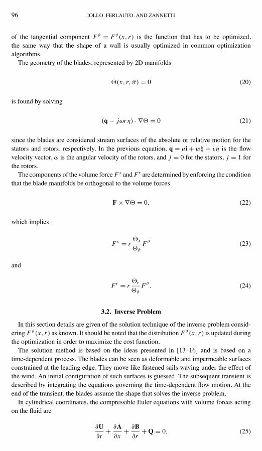
of the tangential component F3 = F3 (x, r) is the function that has to be optimized,the same way that the shape of a wall is usually optimized in common optimizationalgorithms.The geometry of the blades, represented by 2D manifolds

5(x, r,3) = 0 (20)

is found by solving

(q$ j6r4) · )5 = 0 (21)

since the blades are considered stream surfaces of the absolute or relative motion for thestators and rotors, respectively. In the previous equation, q = ui+ w2 + v4 is the flowvelocity vector, 6 is the angular velocity of the rotors, and j = 0 for the stators, j = 1 forthe rotors.The components of the volume force Fx and Fr are determined by enforcing the condition

that the blade manifolds be orthogonal to the volume forces

F')5 = 0, (22)

which implies

Fx = r5x

53

F3 (23)

and

Fr = r5r

53

F3 . (24)

3.2. Inverse Problem

In this section details are given of the solution technique of the inverse problem consid-ering F3 (x, r) as known. It should be noted that the distribution F3 (x, r) is updated duringthe optimization in order to maximize the cost function.The solution method is based on the ideas presented in [13–16] and is based on a

time-dependent process. The blades can be seen as deformable and impermeable surfacesconstrained at the leading edge. They move like fastened sails waving under the effect ofthe wind. An initial configuration of such surfaces is guessed. The subsequent transient isdescribed by integrating the equations governing the time-dependent flow motion. At theend of the transient, the blades assume the shape that solves the inverse problem.In cylindrical coordinates, the compressible Euler equations with volume forces acting

on the fluid are

%U%t

+ %A%x

+ %B%r

+Q = 0, (25)


where

U =

"####$

####%

$

$u$v

$w

e

&####'

####(

A =

"######$

######%

$up + $u2

$uv$uw

u(p + e)

&######'

######(

B =

"######$

######%

$w

$uw$vw

p + $w2

w(p + e)

&######'

######(

Q =

"########$

########%

$wr + $u7

$uwr $ Fx + $u27

2 $vwr $ F8

$(v2$w2)r $ Fr

w(p+e)r $ F · q+ u(p + e)7

&########'

########(

.

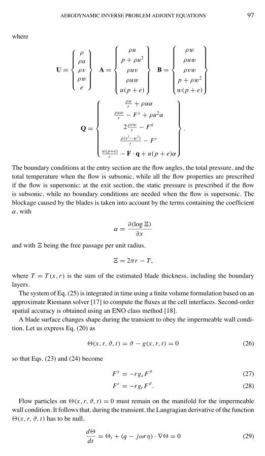
The boundary conditions at the entry section are the flow angles, the total pressure, and thetotal temperature when the flow is subsonic, while all the flow properties are prescribedif the flow is supersonic; at the exit section, the static pressure is prescribed if the flowis subsonic, while no boundary conditions are needed when the flow is supersonic. Theblockage caused by the blades is taken into account by the terms containing the coefficient7, with

7 = %(log9)

%x

and with 9 being the free passage per unit radius,

9 = 2:r $ T,

where T = T (x, r) is the sum of the estimated blade thickness, including the boundarylayers.The system of Eq. (25) is integrated in time using a finite volume formulation based on an

approximate Riemann solver [17] to compute the fluxes at the cell interfaces. Second-orderspatial accuracy is obtained using an ENO class method [18].A blade surface changes shape during the transient to obey the impermeable wall condi-

tion. Let us express Eq. (20) as

5(x, r,3, t) = 3 $ g(x, r, t) = 0 (26)

so that Eqs. (23) and (24) become

Fx = $rgx F3 (27)

Fr = $rgr F3 . (28)

Flow particles on 5(x, r,3, t) = 0 must remain on the manifold for the impermeablewall condition. It follows that, during the transient, the Langragian derivative of the function5(x, r,3, t) has to be null,

d5dt

= 5t + (q $ j6r4) · )5 = 0 (29)


that can be written as

gt = $ugx $ wgr + v $ j6rr

, (30)

with j = 0 for stators and j = 1 for rotors. The above equation is solved coupled to theEuler equations, and it is integrated in time upwinding the spatial derivatives of g accordingto u and w.

3.3. Flow Equations Adjoint

The functional we consider is the conventional thrust expressed as

T (F3 ) =,) rt

rh(p + $u2)r dr

-

out$

,) rt

rh(p + $u2)r dr

-

in=

)

!io

H(U ) d!, (31)

where F3 is the control, while rt and rh are the tip and hub radius, respectively. Themaximum of T is constrained by the steady state Euler equations

E(F3 ) = Ax + Br +Q = 0 (32)

and by the kinematic constraint on the blades

G(U(F3 )) = ugx + wgr $v $ j6r

r= 0. (33)

We introduce the Lagrangian function

L(U, g, F3 ,", µ) =)

!io

H(U) d! +)

&

t"E(U, F3 , g) d&+)

&

µG(U, g) d&, (34)

where t"(x, r) = {'1, '2, '3, '4, '5} and µ = µ(x, r) are Lagrange multipliers. Let uscompute #L. We have

#L = #LU + #LF3 + #Lg + #L" + #Lµ, (35)

with

#LU =)

!io

%H%U

#U d! +)

&

t"#EU d&+)

&

µ%G%U

#U d& (36)

#L" =)

&

t#"E(U, F3 , g) d& (37)

#Lµ =)

&

G(U, g)#µ d& (38)

#LF3 =)

&

t"%Q%F3

#F3 d& (39)

#Lg =)

&

t"#Qg d&+)

&

µ#Gg d&. (40)


The vectors %Q%F3 and

%G%U are easily computed;

%H%U is the derivative of the difference of the

flux component in the x-direction, taken at the inlet and outlet sections.The single contributions of #L must be 0 at the maximum. At the stationary point we

enforce

#LU = 0 #L" = 0 #Lµ = 0 #Lg = 0.

In general this results in #LF3 %= 0. To reach the maximum we take #F3 so that #L =#LF3 > 0, for example using a conjugate gradient method, as explained in the following.We can manipulate Eq. (35), obtaining

#LU =)

!io

%H%U#U d! +

)

(

t"(AUnx + BUnr )#U d) $)

&

( t"xAU + t"rBU )#U d&

+)

&

t"%Q%U#U d&+

)

&

µ%G%U

#U d&, (41)

where( is the entire border of the flow field&, andAU ,BU , andQU are Jacobian matrices.From the condition #LU = 0 we obtain the adjoint of the flow equations and the relativeboundary conditions; that is,

t"xAU + t"rBU $ t"%Q%U$ µ

%G%U

= 0 in & (42)

and,%H(

%U+ t"(AUnx + BUnr )

-#U = 0 on (, (43)

where H ( = H for the inlet and the outlet, and H( = 0 elsewhere.The condition #Lg = 0 yields

#Lg =)

&b

µ#Gg d&+)

&b

t"#Qg d&

=)

(b

µ(q · n)#g d) $)

&b

[(µu)x + (µw)r ]#g d&+)

&b

t"#Qg d& = 0, (44)

where it should be noted that the domain of integration &b and the bounding curve !b arethose relative to the blades. The last integral in the above equation is)

&b

t"#Qg d&=)

&b

t"K)(#g) d&=)

(b

(t"K) · n #g d) $)

&b

) · (t"K)#g d&, (45)

where n = (nx , ny) and

K = r F3

"####$

####%

0 01 00 00 1u w

&####'

####(

.


Hence, the adjoint of the kinematic constraint is

(µu)x + (µw)r $) · (t"K) = 0 in &b (46)

and

[µ(q · n) + (t"K) · n] #g = 0 on !b, (47)

which yields the boundary conditions for Eq. (46) as explained in the following. The adjointequation of the kinematic constraint is coupled to Eq. (42) the same way the kinematicconstraint is coupled to the flow equations.It should be noted that the variations of L with respect to " and µ simply yield the flow

equations and the kinematic constraint respectively.Finally, we are left with

#L = #LF3 =)

&b

t"%Q%F3

#F3 d&. (48)

This functional depends on U, ", µ; these are variables that satisfy the flow equations,the kinematic constraint, and the respective adjoints. Therefore, if we update the presentdistribution of F3 with

#F3 = -t"%Q%F3

,

taking - > 0, then #L > 0. By iterating such a procedure, the maximum is eventuallyreached.This method, namely the gradient method, has a very slow convergence rate. Better

convergence rates are obtained with the conjugate gradient method [21], in which thecorrection to F3 at the iterate k is

(#F3 )k = -

,*t"%Q%F3

+k

$ ;k$1(#F3 )k$1-,

with

;k$1 =

7&b

84t" %Q%F3

5k $4t" %Q

%F35k$194t" %Q

%F35k d&

7&b

84t" %Q

%F35k$192 d&

.

3.3.1. Inlet Boundary Conditions

Let n = (0,$1, 0) at the inlet, so that Eq. (43) reduces to

%H(

%U#U$ t"

%A%U#U = 0. (49)

As the flow variables U have given conditions at the boundaries, the variation #U atthe inlet is such that the boundary conditions on U are still satisfied. For example, if theinlet flow is supersonic, all of the components of U are given. In this case #U = 0 andconsequently there is no boundary condition on ".


In the case of subsonic inlet, four boundary conditions must be provided, for example,

dS = 0, dT o = 0, d) = 0, d< = 0, (50)

where

S = logp$$ 2= log $ (51)

T o = p$

+ =

>(u2 + v2 + w2) = $2=

2

>V 2 + 2=

u5u1

(52)

) = v

u= u3u2

, < = w

u= u4u2

, (53)

where we setU = ($, $u, $v, $w, e) = (u1, u2, u3, u4, u5); = = >$12 ; and > is the specific

heat ratio. We have

"#########$

#########%

#S = %S%u1 #u1 + %S

%u2 #u2 + %S%u3 #u3 + %S

%u4 #u4 + %S%u5 #u5 = 0

#T = %T%u1 #u1 + %T

%u2 #u2 + %T%u3 #u3 + %T

%u4 #u4 + %T%u5 #u5 = 0

#) = %)%u2 #u2 + %)

%u3 #u3 = 0

#< = %<%u2 #u2 + %<

%u4 #u4 = 0.

(54)

By selecting #u2 as the independent variation, we obtain

#U =

"########$

########%

u1V 2u2((1+ > =)V 2 $ 2> =u1u5)

1u3u2u4u2

V 2((1$ 4=2)u1u5 + 2=2V 2)u1u2((1+ > =)V 2 $ 2> =u1u5)

&########'

########(

#u2 = Ji#u2 (55)

from Eq. (54), and we have

,%H(

%U$ t"

%A%U

-Ji#u2 = 0 (56)

from Eq. (49) so that for a generic increment

,%H(

%U$ t"

%A%U

-Ji = 0,

which is a scalar relation that has to be satisfied by the components of ". We have fourconditions for the flow problem, and one for the adjoint equations.


3.3.2. Outlet Boundary Conditions

At the outlet the situation is specular and Eq. (43) still holds. Again, the admissiblevariations #U must satisfy the flow boundary condition. If the regime is supersonic, theoutlet conditions for the flow are determined from the interior and, conversely, the costateequations need five conditions to be prescribed at the exit. We pose " = 0.If the flow is subsonic, one condition has to be supplied for #U, e.g., the static pressure

p at the outlet

p = 2=e $ =$V 2 = constant. (57)

Hence,

#p = %p%u1

#u1 + %p%u2

#u2 + %p%u3

#u3 + %p%u4

#u4 + %p%u5

#u5 = 0, (58)

which gives one of the components of #U, let us say #u5, as a function of the others. Asn = (0, 1, 0), we obtain

,%H(

%U+ t"

%A%U

-Jo

"###$

###%

#u1#u2#u3#u4

&###'

###(= 0, (59)

where J is

Jo =

:

;;;;;<

1 0 0 00 1 0 00 0 1 00 0 0 1$ V 2

2 u v w

=

>>>>>?. (60)

Finally, from Eq. (59), we obtain,%H(

%U+ t"

%A%U

-Jo = 0, (61)

the four boundary conditions for " on the outlet boundary.

3.3.3. Boundary Conditions at the Wall

At the wall we have

t"

*%A%U

nx + %B%U

nr+#U = 0. (62)

The no-through-flow condition at the wall requires the normal velocity component to bezero, so that the above equation becomes

"{0, #pnx , 0, #pnr , 0} = 0 (63)


and finally

'2nx + '4nr = 0. (64)

3.3.4. Kinematic Adjoint Boundary Conditions

#g = 0 at the blade leading edge, and Eq. (47) is satisfied. There is no constraint on #gat the trailing edge; hence we have

[µ(q · n) + (t"K) · n] = 0, (65)

which is the boundary condition for the kinematic adjoint equation at the trailing edge.

3.4. Constraint on Rotor Blades

Rotor blades exchange work with the fluid. When looking for the maximum thrust, wemust keep the work W , performed on the fluid per unit time, constant. The force acting onthe blade is written in the form

F8 (x, r) = f (r)g(x); (66)

therefore the work in the meridional plane per unit time is

W =)

&b

f (r)g(x)6r dr dx =) rt

rhf (r)6c(r)r dr, (67)

where c(r) is the chord of the blade profile and &b is area of the rotor surface projectedonto the meridional plane. In discrete form W can be expressed as

W =M.

i=1f (ri ).(ri ) =

M.

i=1fi.i , (68)

where .(ri ) = 6c(ri )ri (ri $ ri$1) and M is the radial number of the blade discretizationpoints. Posing W = W0, we have

#W =M.

i=1# fi.i = 0. (69)

This equation is satisfied if # f and 0 are orthogonal in the appropriate Euclidean space.The variation of Lagrangian Eq. (48) is written as

#L =),#F8 d&, , = t"

%Q%F3

, (70)

and in discrete form we have

#L =.

,i# fi . (71)


Aswe are searching for themaximum thrust, wemust choose the controls # fi so that Eq. (69)is verified and the increment #L =

/,i# fi assumes its highest positive value. As in the

diffuser case, we obtain

# fi = -

0

1,iM.

j=1.2j $ .i

M.

j=1, j. j

2

3. (72)

4. ADJOINT EQUATION NUMERICAL SOLUTION

The numerical solution of the adjoint equations is obtained by using a first-order time-dependent technique based on a finite volume discretization. The solver computes the fluxesat cell interfaces using a flux-vector splitting technique. In a similar way, the boundaryconditions are imposed on the numerical fluxes at the computational field edges.Let us consider the adjoint equations. If a time derivative t"? is added to Eqs. (42) and

(43), we are led to the hyperbolic system

t"? $ t"xAU $ t"rBU + t"QU + µGU = 0. (73)

This system is linear, because AU,BU,QU, and GU only depend on x and r , and its char-acteristics are the same as those of the flow problem, but with opposite speeds.In order to take advantage of a finite volume formulation which is similar to that used

for the flow equations, we set

t"xAU = (t"AU)x $ t"(AU)x (74)t"rBU = (t"BU)r $ t"(BU)x , (75)

and then, substituting in Eq. (73), we have

t"? $ [t"AU ]x $ [t"BU ]r + t"[(AU )x + (BU )r ]+ t"QU + µGU = 0. (76)

Considering an elementary volume of integration 6 with surface ) , we rewrite Eq. (76) inconservation form and apply the Gauss theorem to obtain

%

%?

)

6

t" d&$)

)

t"C d) + t"

)

)

C d) +)

6

(t"QU + µGU) d6 = 0, (77)

with C = AUnx + BUnr . In the previous formula we considered " as piecewise constantover the discretization volume. A characteristic-based approach is used to evaluate theconvective fluxes at the cell interfaces. The total flux across the interface (int) is evaluatedas the sum of two contributions which arise from the left (l) and right (r ) sides of theinterface, according to the wave-propagating nature of the hyperbolic system

(t"C)int = (t"+C+)l + (t"$C$)r , (78)

where

C+ = LD+R, C$ = LD$R, (79)


and D+ + D$ = D. The matrix D is

D =

0

@@@@@@1

Vn 0 0 0 00 Vn 0 0 00 0 Vn 0 00 0 0 Vn $ a 00 0 0 0 Vn + a

2

AAAAAA3. (80)

The matrices D+ and D$ are diagonal as well and they consist of the positive and negativeeigenvalues of C , respectively.The adjoint system Eq. (46) for the kinematical constraint can bemanipulated in a similar

way. By adding a time derivative µ? we have

µ? $ (µu)x $ (µw)r + ) · (t"K) = 0. (81)

Once again the sign of the time derivate has been chosen in order to obtain a well posedproblem. The finite volume approximation is straightforward;

%

%?

)

6b

µ d6 $)

>b

µ(unx + wnr ) d! +)

>b

(t"K) · n d! = 0, (82)

where6b is the projection of the blade surface onto the meridional plane, and >b its contour.The flux µ(unx + wnr ) at the cell interfaces is taken upwind.

5. RESULTS

In the following sections we present the results for the diffuser test case and for theturbo-machinery model in the meridional plane. The grids we employ are rather coarse, asthe solved flow problems do not require additional resolution. In the diffuser case we showthat the results are basically unaffected by a finer grid and a larger design space.In order to show convergence and consistency of the approach presented in the previous

sections, we made sure that the gradient becomes negligible. We therefore pursued opti-mization steps far beyond the point where the functional has a substantial decrease: Wereached O(10,000) optimization steps. For applications, only 50–100 optimization stepsare acceptable. Within these limits we have reached a substantial decrease in the functionalin all the illustrated cases. After the first few optimization steps, the corrections to the flowas well as to the adjoint solution also become so small that only a few relaxation steps in therespective solvers are needed for convergence. The most expensive case presented, the twocounterrotating rotors, requires about 20 h of CPU time on a Digital Alpha 600Workstationafter 10,000 optimization steps.

5.1. Diffuser

The diffuser is discretized over a 40' 20 grid. The inlet pressure is pin = 0.83, the outletpressure pout = 0.944. The imposed flow angle at the inlet varies from zero, at the bottomwall, to 10 degrees, at the upper wall. We are looking for the diffuser geometry that bestapproximates a zero flow angle at the outlet. As explained, the control is represented hereby the pressure gradient at each computational point lying on the upper wall. The numberof design variables is one less than the grid discretization in the x-direction. If a usual shape


optimization method were to be applied in this case, we would obtain an additional adjointpartial differential equation. The initial wall pressure distribution is a parabolic profile (seeFig. 6) that satisfies the constraint on the pressure gradient in Fig. 1.The initial and final geometry of the diffuser are depicted in Fig. 3. The initial geometry

is characterized by a nonzero flow angle ) (y)out at the exit. The l2 norm of the gradient

FIG. 3. Diffuser. The geometry and pressure field before (Top) and after (Bottom) the optimization process.


FIG. 4. Diffuser. Gradient residual res versus optimization step n.

residuals is presented in Fig. 4. The functional D decreases noticeably (see Fig. 5), butbecause of the pressure gradient constraint, the flow is not perfectly axial at the outlet.The pressures displayed in Fig. 6 are relative to the cell centers next to the diffuser wall.

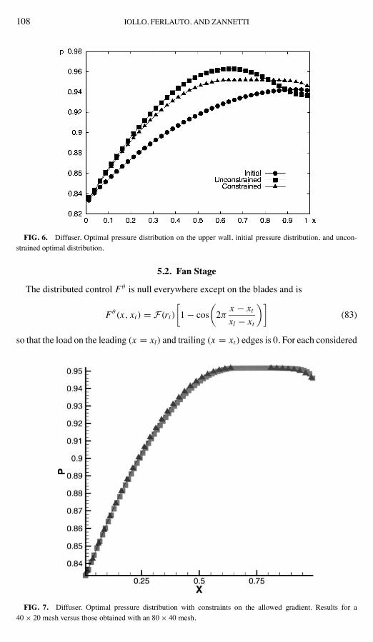
The initial and optimal configurations are shown. The unconstrained optimal wall pressuredistribution is depicted in the same figure. The small outlet pressure differences are due tothe various geometries pertinent to each case.The used mesh makes the problem computationally quite small. Indeed, in such a simple

problem there are 40 design variables with strictly enforced inequality constraints on thepressure gradient. We have increased the spatial resolution to 80' 40 grid points, thususing 80 design variables. Even when the design space is doubled, the results obtained, interms of the pressure distribution, do not remarkably change, as seen in Fig. 7.

FIG. 5. Diffuser. Flow alignment D versus optimization step n.


FIG. 6. Diffuser. Optimal pressure distribution on the upper wall, initial pressure distribution, and uncon-strained optimal distribution.

5.2. Fan Stage

The distributed control F8 is null everywhere except on the blades and is

F8 (x, xi ) = F(ri ),1$ cos

*2:

x $ xtxl $ xt

+-(83)

so that the load on the leading (x = xl) and trailing (x = xt ) edges is 0. For each considered

FIG. 7. Diffuser. Optimal pressure distribution with constraints on the allowed gradient. Results for a40' 20 mesh versus those obtained with an 80' 40 mesh.


FIG. 8. Fan stage. Gradient residual versus optimization steps.

blade, we have as many design parameters F(ri ) as the number of computational points inthe radial direction.Therefore, Eq. (48) is discretized as

#L =.

i

#F(ri )L(ri )(ri $ ri$1), (84)

where

L(ri ) =.

j

t"(ri , x j )%Q%F3

(ri , x j ),1$ cos

*2:

x j $ xtxl $ xt

+-(x j $ x j$1).

The design variables for this test case, where the grid is 60' 24, are 24 for the stator and

FIG. 9. Fan stage. Thrust versus optimization steps.


FIG. 10. Counterrotating rotors. Initial force distribution Fi on the blade.

24 for the rotor; 6 = 1.58 and on the rotor the work is fixed to that relative to the initialforce distribution. The constraint on the total work performed by the rotor allows verysmall variations of the force distribution on the rotor itself. This is seen in the gradientcomponents relative to the rotor which are two orders of magnitude smaller than thoserelative to the stator. In a different test case relative to a single rotor but not shown here, wefound that for a gradient residual decrease of two orders of magnitude, the thrust gain is verylimited.In the initial configuration, the stator does not exert any force on the flow, that is, it

coincides with a force-free stream surface. The gradient residual in Fig. 8 and the thrust inFig. 9 are plotted against the optimization step. After the computation of the first flow and

FIG. 11. Final force distribution.


adjoint fields, each optimization step takes a significantly reduced amount of computationaltime. The gradient decreases by more than two orders of magnitude and the thrust increasesby about 100%.We consider an additional test case belonging to the same class of problem; two coun-

terrotating ducted fans. The counterrotating fan case is discretized on a 75' 25 grid, with

FIG. 12. Counterrotating rotors. Initial geometry.


24' 2 design variables. Again the total work performed by the rotors is fixed and equalto that of the initial force configuration. The two rotation speeds are 61 = $62 = 0.4. Theinitial force radial distribution is constant on both blades. The thrust increases from 0.0235to 0.0285 and reaches its asymptotic value after 20 design cycles. The computation waspursued until the gradient was reduced by three orders of magnitude. The solution of themaximum thrust is one with minimal axial deviation at the exit, and a force radial distri-bution quite far from the initial guess. We show the initial and final force configurations inFigs. 10 and 11. The solution in terms of force distribution is symmetric as expected. Theinitial and final geometries of the blades are presented in Figs. 12 and 13.

FIG. 13. Counterrotating rotors. Final geometry.


6. CONCLUSIONS

In this work we derive an adjoint optimization method for aerodynamic design basedon the solution of the inverse problem. We apply it to diffuser and turbo-machinery de-sign. It takes advantage of the inverse solution of the flow equations to determine optimalconfigurations. The flow constraints are imposed directly into the parameterization of theflow distribution that has to be optimized. No additional Lagrange multipliers are neededto satisfy such constraints. The relative advantages of using this approach compared to theusual shape design optimization should be evaluated case by case considering the numberof flow constraints versus the number of geometric constraints. We believe this approachto be more efficient for aerodynamic components where the flow quality is crucial.

APPENDIX

AU =

:

;;;;;;<

0 1 0 0 0=V 2 $ u2 $2(= $ 1)u $2=v $2=w 2=$uv v u 0 0$uw w 0 u 0

u42=V 2 $ > e

$

5> e$$ =(V 2 + 2u2) $2=uv $2=uw > u

=

>>>>>>?(85)

BU =

:

;;;;;;;<

0 0 0 1 0$uw w 0 u 0$vw 0 w v 0

=V 2 $ w2 $2=u $2=v $2(= $ 1)w 2=

w42=V 2 $ > e

$

5$2=uw $2=vw > e

$$ =(V 2 + 2w2) >w

=

>>>>>>>?

(86)

QU =

:

;;;;;;;;<

0 7 0 1r 0

$ uwr $

u7$

wr + 2u7 0 u

r 0

$ 2vwr 0 2w

r2vr 0

w2 $ v2

r 0 2vr $ 2wr 0

q51 q52 q53 q54 > wr + u7

=

>>>>>>>>?

(87)

q51 = $ F8

$(urgx + wrgr $ v)$

*> e$$ 2=V 2

+*w

r+ u7

+(88)

q52 = F8

$rgx + 7

*> e$$ =V 2

+$ 2=

*w

r+ u7

+(89)

q53 = $ F8

$+ 2=v

*w

r+ u7

+(90)

q54 = F8

$rgr + 1

r

*> e$$ 2=V 2

+$ 2=w

*w

r+ u7

+(91)

%Q%F8

= {0, rgx , $1, rgr , rgxu + rgrw $ v} (92)


%H%U

= {0, gx , $1r, gr , 0} (93)

%H (

%U= {=V 2 $ u2, $2(= $ 1)u, $2=v, $2=w, 2=} (94)

L =

:

;;;;;;;;;<

1$ =V 2a2

2=ua2

2=va2

2=wa2

2=a2

Vt$

nr$

0 nx$

0

$ v$

0 $ 1$

0 0=V 2 $ aVn

2a2anx $ 2=u2a2 $ =v

a2anr $ 2=w

2a2=a2

aVn + 2=V 22a2 $ anx + 2=u

2a2 $ =va2 $

anr + 2=w2a2

=a2

=

>>>>>>>>>?

(95)

R =

:

;;;;;;;<

1 0 0 1 1u $nr 0 u + anx u $ anxv 0 $ v v

w $$nx 0 w + anr w $ anrV 22 $Vt $v a2 + =V 2

2k + aVn a2 + =V 22k $ aVn

=

>>>>>>>?

. (96)

REFERENCES

1. W. Mangler, Die berechnung eines tragflugelprofiles mit vorgeschriebener druckverteilung, Jahrb. Deutsch.Luftfahrtforschung 1, 46 (1938).

2. J. M. Lighthill, A New Method of Two-Dimensional Aerodynamic Design, Aeronautics Research CouncilReports and Memoranda 2112 (1945).

3. A. M. Elizarov, N. B. Il’inskiy, and A. V. Potashev, Mathematical Methods of Airfoil Design (AkademieVerlag, Berlin, 1997).

4. L. Polito, Un Metodo Esatto per il Progetto di Profili Alari in Corrente Incompressibile Aventi un Presta-bilito Andamento della Velocia sul Contorno, Universita di Pisa, Rapporto Istituto di Aeronautica 42(1974).

5. F. Bauer, P. Garabedian, and D. Korn, Supercritical Wing Sections (Springer-Verlag, Berlin/New York,1972).

6. G. Volpe, Geometric and Surface Pressure Restrictions in Airfoil Design, AGARD-R-780 (1990).7. O. Pironneau, On optimum design in fluid mechanics, J. Fluid Mech. 59, 117 (1972).8. A. Jameson, Aerodynamic Design via Control Theory, ICASE Report, 88–64; J. Sci. Comput. 3, 233(1988).

9. A. Jameson, Optimum aerodynamic design using control theory, in Computational Fluid Dynamics Review,edited by M. Hafez (John Wiley & Sons, 1995) p. 495.

10. A. Jameson, L.Martinelli, andN. A. Pierce, Optimum aerodynamic design using theNavier–Stokes equations,Theoret. Comput. Fluid Dynam. 10, 213 (1998).

11. R. F. van den Dam, J. A. van Egmond, and J. W. Sloof, Optimization of Target Pressure Distributions,AGARD-R-780 (1990).

12. J. Elliot and J. Peraire Constrained, multipoint shape optimization for complex 3D configurations, Aeronaut.J. Aug./Sept. 365 (1998).

13. C. Bena, F. Larocca, and L. Zannetti, Design ofmultistage axial flow turbines and compressors, in IMech-E 3rdEuropean Conference on Turbomachinery Proceedings, London, 1999 (Professional Engineering Publishers,London, 1999) p. 635.

14. B. S. Stratford, The prediction of separation of the turbulent boundary layer, J. Fluid Mech. 5, 1 (1954).


15. L. Zannetti, A time-dependent method to solve the inverse problem for internal flows, AIAA J. 18, 754(1980).

16. L. Zannetti and F. Larocca, Inverse Methods for 3D Internal Flows, AGARD-R-780 (1990).17. M. Pandolfi, A contribution to the numerical prediction of unsteady flows, AIAA J. 22, 602 (1984).18. A. Harten, B. Engquist, and S. Osher, Uniformly High-order-accurate essentially nonoscillatory schemes, III,

J. Comput. Phys. 71, 231 (1987).19. F. Beux and A. Dervieux, Exact-gradient shape optimization of a 2-D Euler flow, Finite Elem. Anal. Design

12, 281 (1992).20. A. Iollo andM. D. Salas, Contribution to the optimal shape design of 2D internal flows with embedded shocks,

J. Comput. Phys. 125, 124 (1996).21. R. Fletcher, Practical Methods of Optimization (Wiley, New York, 1980).

Documents

An Aerodynamic Optimization Method Based on the …aiollo/Papers_files/Journal of... · An Aerodynamic Optimization Method Based on the Inverse Problem ... at the wall is optimized