Embed Size (px)
Citation preview

Amber 2016Reference Manual(Covers Amber16 and AmberTools16)


Amber 2016Reference Manual
(Covers Amber16 and AmberTools16)
Principal contributors to the current codes:
David A. Case (Rutgers)Ross C. Walker (SDSC, UCSD)Thomas E. Cheatham III (Utah)
Carlos Simmerling (Stony Brook)Adrian Roitberg (Florida)
Kenneth M. Merz (Michigan State)Ray Luo (UC Irvine)
Tom Darden (OpenEye)Junmei Wang (UT Southwestern Medical Center)
Robert E. Duke (NIEHS)Daniel R. Roe (Utah)
Scott LeGrand (Amazon)Jason Swails (Rutgers)
David Cerutti (Michigan State)Gérald Monard (U. Lorraine)
Celeste Sagui (NCSU)Joe Kaus (UCSD)
Robin Betz (UCSD)Ben Madej (UCSD)Charles Lin (UCSD)
Daniel Mermelstein (UCSD)Pengfei Li (Michigan State)
Alexey Onufriev (Virginia Tech)Saeed Izadi (Virginia Tech)Romain M. Wolf (Novartis)
Xiongwu Wu (NIH)Andreas W. Götz (SDSC, UCSD)
Holger Gohlke (Düsseldorf)Nadine Homeyer (Düsseldorf)
Wesley M. Botello-Smith (UC Irvine)Li Xiao (UC Irvine)
Tyler Luchko (Rutgers)Tim Giese (Rutgers)
Taisung Lee (Rutgers)Hung T. Nguyen (Rutgers)
Hai Nguyen (Stony Brook, Rutgers)Pawel Janowski (Rutgers)
Igor Omelyan (NINT)Andriy Kovalenko (NINT)
Peter A. Kollman (UC San Francisco)
For more information, please visit http://ambermd.org/contributors.html
3

Acknowledgments
Research support from DARPA, NIH, ONR, DOE and NSF is gratefully acknowledged, along with supportfrom NVIDIA, Amazon and Exxact. Many people helped add features to various codes; these contributions aredescribed in the documentation for the individual programs; see also http://ambermd.org/contributors.html.
Recommended Citation:
• When citing Amber 2016 (comprised of AmberTools16 and Amber16) in the literature, the following citationshould be used:
D.A. Case, R.M. Betz, D.S. Cerutti, T.E. Cheatham, III, T.A. Darden, R.E. Duke, T.J. Giese, H. Gohlke,A.W. Goetz, N. Homeyer, S. Izadi, P. Janowski, J. Kaus, A. Kovalenko, T.S. Lee, S. LeGrand, P. Li, C.Lin, T. Luchko, R. Luo, B. Madej, D. Mermelstein, K.M. Merz, G. Monard, H. Nguyen, H.T. Nguyen, I.Omelyan, A. Onufriev, D.R. Roe, A. Roitberg, C. Sagui, C.L. Simmerling, W.M. Botello-Smith, J. Swails,R.C. Walker, J. Wang, R.M. Wolf, X. Wu, L. Xiao and P.A. Kollman (2016), AMBER 2016, University ofCalifornia, San Francisco.
Peter Kollman died unexpectedly in May, 2001. We dedicate Amber to his memory.
Notes
• We thank Chris Bayly and Merck-Frosst, Canada for permission to include charge increments for the AM1-BCC charge scheme.
• Some of the force field routines were adapted from similar routines in the MOIL program package: R. Elber,A. Roitberg, C. Simmerling, R. Goldstein, H. Li, G. Verkhivker, C. Keasar, J. Zhang and A. Ulitsky, "MOIL:A program for simulations of macromolecules" Comp. Phys. Commun. 91, 159-189 (1995).
Cover illustration: Painting by Giulia Palermo (UCSD) of a two-metal ion mechanism in Type II topoisomerase,as observed from molecular simulations. (Palermo et al. Acc. Chem. Res. 48, 220-228, 2015). Magnesium ionsare shown as yellow spheres with protein (violet) and the DNA (green/blue) as ribbons. The picture was paintedusing a combination of pastels and oil colors.
4

Contents
Contents 5
I. Introduction and Installation 13
1. Introduction 151.1. Information flow in Amber . . . . . . . . . . . . . . . . . . . . . . . . . . . . . . . . . . . . . . 151.2. List of programs . . . . . . . . . . . . . . . . . . . . . . . . . . . . . . . . . . . . . . . . . . . . 18
2. Installation 232.1. Uninstalling and cleaning . . . . . . . . . . . . . . . . . . . . . . . . . . . . . . . . . . . . . . . 252.2. Python in Amber . . . . . . . . . . . . . . . . . . . . . . . . . . . . . . . . . . . . . . . . . . . 262.3. Applying Updates . . . . . . . . . . . . . . . . . . . . . . . . . . . . . . . . . . . . . . . . . . . 282.4. Contacting the developers . . . . . . . . . . . . . . . . . . . . . . . . . . . . . . . . . . . . . . . 29
II. Amber force fields 31
3. Molecular mechanics force fields 333.1. Proteins . . . . . . . . . . . . . . . . . . . . . . . . . . . . . . . . . . . . . . . . . . . . . . . . 343.2. Nucleic acids . . . . . . . . . . . . . . . . . . . . . . . . . . . . . . . . . . . . . . . . . . . . . 373.3. Carbohydrates . . . . . . . . . . . . . . . . . . . . . . . . . . . . . . . . . . . . . . . . . . . . . 393.4. Lipids . . . . . . . . . . . . . . . . . . . . . . . . . . . . . . . . . . . . . . . . . . . . . . . . . 463.5. Solvents . . . . . . . . . . . . . . . . . . . . . . . . . . . . . . . . . . . . . . . . . . . . . . . . 473.6. Ions . . . . . . . . . . . . . . . . . . . . . . . . . . . . . . . . . . . . . . . . . . . . . . . . . . 493.7. Modified amino acids and nucleotides . . . . . . . . . . . . . . . . . . . . . . . . . . . . . . . . 513.8. Force fields related to semi-empirical QM . . . . . . . . . . . . . . . . . . . . . . . . . . . . . . 513.9. Obsolete force field files . . . . . . . . . . . . . . . . . . . . . . . . . . . . . . . . . . . . . . . 51
4. The Generalized Born/Surface Area Model 554.1. GB/SA input parameters . . . . . . . . . . . . . . . . . . . . . . . . . . . . . . . . . . . . . . . 574.2. ALPB (Analytical Linearized Poisson-Boltzmann) . . . . . . . . . . . . . . . . . . . . . . . . . 60
5. GBNSR6 625.1. GB equations available in gbnsr6 . . . . . . . . . . . . . . . . . . . . . . . . . . . . . . . . . . . 625.2. Numerical implementation of the R6 integral . . . . . . . . . . . . . . . . . . . . . . . . . . . . 635.3. Usage . . . . . . . . . . . . . . . . . . . . . . . . . . . . . . . . . . . . . . . . . . . . . . . . . 63
6. PBSA 666.1. Introduction . . . . . . . . . . . . . . . . . . . . . . . . . . . . . . . . . . . . . . . . . . . . . . 666.2. Usage and keywords . . . . . . . . . . . . . . . . . . . . . . . . . . . . . . . . . . . . . . . . . 696.3. Example inputs and demonstrations of functionalities . . . . . . . . . . . . . . . . . . . . . . . . 786.4. Visualization functions in pbsa . . . . . . . . . . . . . . . . . . . . . . . . . . . . . . . . . . . . 806.5. pbsa in sander and NAB . . . . . . . . . . . . . . . . . . . . . . . . . . . . . . . . . . . . . . . 87
5

CONTENTS
7. Reference Interaction Site Model 907.1. Introduction . . . . . . . . . . . . . . . . . . . . . . . . . . . . . . . . . . . . . . . . . . . . . . 907.2. Practical Considerations . . . . . . . . . . . . . . . . . . . . . . . . . . . . . . . . . . . . . . . 957.3. Work Flow . . . . . . . . . . . . . . . . . . . . . . . . . . . . . . . . . . . . . . . . . . . . . . 967.4. rism1d . . . . . . . . . . . . . . . . . . . . . . . . . . . . . . . . . . . . . . . . . . . . . . . . . 987.5. 3D-RISM in NAB . . . . . . . . . . . . . . . . . . . . . . . . . . . . . . . . . . . . . . . . . . . 1017.6. rism3d.snglpnt . . . . . . . . . . . . . . . . . . . . . . . . . . . . . . . . . . . . . . . . . . . 1037.7. 3D-RISM in sander . . . . . . . . . . . . . . . . . . . . . . . . . . . . . . . . . . . . . . . . . . 1067.8. RISM File Formats . . . . . . . . . . . . . . . . . . . . . . . . . . . . . . . . . . . . . . . . . . 114
8. Empirical Valence Bond 1208.1. Introduction . . . . . . . . . . . . . . . . . . . . . . . . . . . . . . . . . . . . . . . . . . . . . . 1208.2. General usage description . . . . . . . . . . . . . . . . . . . . . . . . . . . . . . . . . . . . . . . 1218.3. Biased sampling . . . . . . . . . . . . . . . . . . . . . . . . . . . . . . . . . . . . . . . . . . . . 1238.4. Quantization of nuclear degrees of freedom . . . . . . . . . . . . . . . . . . . . . . . . . . . . . 1268.5. Distributed Gaussian EVB . . . . . . . . . . . . . . . . . . . . . . . . . . . . . . . . . . . . . . 1268.6. EVB input variables and interdependencies . . . . . . . . . . . . . . . . . . . . . . . . . . . . . 128
9. sqm: Semi-empirical quantum chemistry 1339.1. Available Hamiltonians . . . . . . . . . . . . . . . . . . . . . . . . . . . . . . . . . . . . . . . . 1339.2. Dispersion and hydrogen bond correction . . . . . . . . . . . . . . . . . . . . . . . . . . . . . . 1349.3. Usage . . . . . . . . . . . . . . . . . . . . . . . . . . . . . . . . . . . . . . . . . . . . . . . . . 135
10. QM/MM calculations 14110.1. Built-in semiempirical NDDO methods and SCC-DFTB . . . . . . . . . . . . . . . . . . . . . . 14110.2. Interface for ab initio and DFT methods . . . . . . . . . . . . . . . . . . . . . . . . . . . . . . . 15010.3. Adaptive solvent QM/MM simulations . . . . . . . . . . . . . . . . . . . . . . . . . . . . . . . . 16210.4. Adaptive buffered force-mixing QM/MM . . . . . . . . . . . . . . . . . . . . . . . . . . . . . . 16810.5. SEBOMD: SemiEmpirical Born-Oppenheimer Molecular Dynamics . . . . . . . . . . . . . . . . 175
11. paramfit 18011.1. Usage . . . . . . . . . . . . . . . . . . . . . . . . . . . . . . . . . . . . . . . . . . . . . . . . . 18111.2. The Job Control File . . . . . . . . . . . . . . . . . . . . . . . . . . . . . . . . . . . . . . . . . 18211.3. Multiple molecule fits . . . . . . . . . . . . . . . . . . . . . . . . . . . . . . . . . . . . . . . . . 18811.4. Fitting Forces . . . . . . . . . . . . . . . . . . . . . . . . . . . . . . . . . . . . . . . . . . . . . 18811.5. Examples . . . . . . . . . . . . . . . . . . . . . . . . . . . . . . . . . . . . . . . . . . . . . . . 189
III. System preparation 191
12. Preparing PDB Files 19312.1. Cleaning up Protein PDB Files for AMBER . . . . . . . . . . . . . . . . . . . . . . . . . . . . . 19312.2. Residue naming conventions . . . . . . . . . . . . . . . . . . . . . . . . . . . . . . . . . . . . . 19412.3. Chains, Residue Numbering, Missing Residues . . . . . . . . . . . . . . . . . . . . . . . . . . . 19512.4. pdb4amber . . . . . . . . . . . . . . . . . . . . . . . . . . . . . . . . . . . . . . . . . . . . . . 19512.5. reduce . . . . . . . . . . . . . . . . . . . . . . . . . . . . . . . . . . . . . . . . . . . . . . . . . 198
13. LEaP 19913.1. Introduction . . . . . . . . . . . . . . . . . . . . . . . . . . . . . . . . . . . . . . . . . . . . . . 19913.2. Concepts . . . . . . . . . . . . . . . . . . . . . . . . . . . . . . . . . . . . . . . . . . . . . . . 19913.3. Running LEaP . . . . . . . . . . . . . . . . . . . . . . . . . . . . . . . . . . . . . . . . . . . . . 20313.4. Basic instructions for using LEaP to build molecules . . . . . . . . . . . . . . . . . . . . . . . . 20813.5. Commands . . . . . . . . . . . . . . . . . . . . . . . . . . . . . . . . . . . . . . . . . . . . . . 20913.6. Building oligosaccharides, lipids and glycoproteins . . . . . . . . . . . . . . . . . . . . . . . . . 226
6
CONTENTS
14. Reading and modifying Amber parameter files 23414.1. Understanding Amber parameter files . . . . . . . . . . . . . . . . . . . . . . . . . . . . . . . . 23414.2. ParmEd . . . . . . . . . . . . . . . . . . . . . . . . . . . . . . . . . . . . . . . . . . . . . . . . 242
15. Antechamber and GAFF 27015.1. Principal programs . . . . . . . . . . . . . . . . . . . . . . . . . . . . . . . . . . . . . . . . . . 27015.2. A simple example for antechamber . . . . . . . . . . . . . . . . . . . . . . . . . . . . . . . . . . 27515.3. Using the components.cif file from the PDB . . . . . . . . . . . . . . . . . . . . . . . . . . . . . 27815.4. Programs called by antechamber . . . . . . . . . . . . . . . . . . . . . . . . . . . . . . . . . . . 27815.5. Miscellaneous programs . . . . . . . . . . . . . . . . . . . . . . . . . . . . . . . . . . . . . . . 28215.6. New Development of Antechamber And GAFF . . . . . . . . . . . . . . . . . . . . . . . . . . . 28515.7. Metal Center Parameter Builder (MCPB) . . . . . . . . . . . . . . . . . . . . . . . . . . . . . . 28615.8. Python Metal Site Modeling Toolbox (pyMSMT) . . . . . . . . . . . . . . . . . . . . . . . . . . 287
16. Setting up crystal simulations 29716.1. UnitCell . . . . . . . . . . . . . . . . . . . . . . . . . . . . . . . . . . . . . . . . . . . . . . . . 29716.2. PropPDB . . . . . . . . . . . . . . . . . . . . . . . . . . . . . . . . . . . . . . . . . . . . . . . 29716.3. AddToBox . . . . . . . . . . . . . . . . . . . . . . . . . . . . . . . . . . . . . . . . . . . . . . . 29716.4. ChBox . . . . . . . . . . . . . . . . . . . . . . . . . . . . . . . . . . . . . . . . . . . . . . . . . 299
17. Using the AMOEBA Force Field with AMBER 30017.1. Installing TINKER . . . . . . . . . . . . . . . . . . . . . . . . . . . . . . . . . . . . . . . . . . 30017.2. Preparing the system with TINKER . . . . . . . . . . . . . . . . . . . . . . . . . . . . . . . . . 301
IV. Running simulations 303
18. sander 30518.1. Introduction . . . . . . . . . . . . . . . . . . . . . . . . . . . . . . . . . . . . . . . . . . . . . . 30518.2. File usage . . . . . . . . . . . . . . . . . . . . . . . . . . . . . . . . . . . . . . . . . . . . . . . 30618.3. Example input files . . . . . . . . . . . . . . . . . . . . . . . . . . . . . . . . . . . . . . . . . . 30718.4. Namelist Input Syntax . . . . . . . . . . . . . . . . . . . . . . . . . . . . . . . . . . . . . . . . 30818.5. Overview of the information in the input file . . . . . . . . . . . . . . . . . . . . . . . . . . . . . 30918.6. General minimization and dynamics parameters . . . . . . . . . . . . . . . . . . . . . . . . . . . 30918.7. Potential function parameters . . . . . . . . . . . . . . . . . . . . . . . . . . . . . . . . . . . . . 32018.8. Varying conditions . . . . . . . . . . . . . . . . . . . . . . . . . . . . . . . . . . . . . . . . . . 32618.9. File redirection commands . . . . . . . . . . . . . . . . . . . . . . . . . . . . . . . . . . . . . . 33018.10.Getting debugging information . . . . . . . . . . . . . . . . . . . . . . . . . . . . . . . . . . . . 33018.11.multisander (and multipmemd) . . . . . . . . . . . . . . . . . . . . . . . . . . . . . . . . . . . . 33318.12.Programmer’s Corner: The sander API . . . . . . . . . . . . . . . . . . . . . . . . . . . . . . . . 334
19. pmemd 35519.1. Introduction . . . . . . . . . . . . . . . . . . . . . . . . . . . . . . . . . . . . . . . . . . . . . . 35519.2. Functionality . . . . . . . . . . . . . . . . . . . . . . . . . . . . . . . . . . . . . . . . . . . . . 35519.3. PMEMD-specific namelist variables . . . . . . . . . . . . . . . . . . . . . . . . . . . . . . . . . 35719.4. Slightly changed functionality . . . . . . . . . . . . . . . . . . . . . . . . . . . . . . . . . . . . 35819.5. Parallel performance tuning and hints . . . . . . . . . . . . . . . . . . . . . . . . . . . . . . . . 35919.6. GPU Accelerated PMEMD . . . . . . . . . . . . . . . . . . . . . . . . . . . . . . . . . . . . . . 35919.7. Intel® Many Integrated Core Architecture . . . . . . . . . . . . . . . . . . . . . . . . . . . . . . 365
20. Atom and Residue Selections 37120.1. Amber Masks . . . . . . . . . . . . . . . . . . . . . . . . . . . . . . . . . . . . . . . . . . . . . 37120.2. "Atom Expressions" in NAB Applications . . . . . . . . . . . . . . . . . . . . . . . . . . . . . . 37420.3. GROUP Specification . . . . . . . . . . . . . . . . . . . . . . . . . . . . . . . . . . . . . . . . . 374
7
CONTENTS
21. Sampling configuration space 37821.1. Self-Guided Langevin dynamics . . . . . . . . . . . . . . . . . . . . . . . . . . . . . . . . . . . 37821.2. Accelerated Molecular Dynamics . . . . . . . . . . . . . . . . . . . . . . . . . . . . . . . . . . . 38121.3. Gaussian Accelerated Molecular Dynamics . . . . . . . . . . . . . . . . . . . . . . . . . . . . . 38421.4. Targeted MD . . . . . . . . . . . . . . . . . . . . . . . . . . . . . . . . . . . . . . . . . . . . . 38721.5. Multiply-Targeted MD (MTMD) . . . . . . . . . . . . . . . . . . . . . . . . . . . . . . . . . . . 38821.6. Nudged elastic band calculations . . . . . . . . . . . . . . . . . . . . . . . . . . . . . . . . . . . 38921.7. Low-MODe (LMOD) methods . . . . . . . . . . . . . . . . . . . . . . . . . . . . . . . . . . . . 393
22. Free energies 39722.1. Thermodynamic integration . . . . . . . . . . . . . . . . . . . . . . . . . . . . . . . . . . . . . . 39722.2. Absolute Free Energies using EMIL . . . . . . . . . . . . . . . . . . . . . . . . . . . . . . . . . 40622.3. Linear Interaction Energies . . . . . . . . . . . . . . . . . . . . . . . . . . . . . . . . . . . . . . 41022.4. Umbrella sampling . . . . . . . . . . . . . . . . . . . . . . . . . . . . . . . . . . . . . . . . . . 41122.5. Replica Exchange Molecular Dynamics (REMD) . . . . . . . . . . . . . . . . . . . . . . . . . . 41222.6. Adaptively biased MD, steered MD, and umbrella sampling with REMD . . . . . . . . . . . . . . 42922.7. Steered Molecular Dynamics (SMD) and the Jarzynski Relationship . . . . . . . . . . . . . . . . 436
23. Constant pH calculations 44023.1. Background . . . . . . . . . . . . . . . . . . . . . . . . . . . . . . . . . . . . . . . . . . . . . . 44023.2. Preparing a system for constant pH . . . . . . . . . . . . . . . . . . . . . . . . . . . . . . . . . . 44023.3. Running at constant pH . . . . . . . . . . . . . . . . . . . . . . . . . . . . . . . . . . . . . . . . 44223.4. Analyzing constant pH simulations . . . . . . . . . . . . . . . . . . . . . . . . . . . . . . . . . . 44523.5. Extending constant pH to additional titratable groups . . . . . . . . . . . . . . . . . . . . . . . . 44723.6. Constant pH MD Replica Exchange . . . . . . . . . . . . . . . . . . . . . . . . . . . . . . . . . 44823.7. cphstats . . . . . . . . . . . . . . . . . . . . . . . . . . . . . . . . . . . . . . . . . . . . . . . . 448
24. NMR, X-ray, and cryo-EM/ET refinement 45624.1. Distance, angle and torsional restraints . . . . . . . . . . . . . . . . . . . . . . . . . . . . . . . . 45724.2. NOESY volume restraints . . . . . . . . . . . . . . . . . . . . . . . . . . . . . . . . . . . . . . 46224.3. Chemical shift restraints . . . . . . . . . . . . . . . . . . . . . . . . . . . . . . . . . . . . . . . 46324.4. Pseudocontact shift restraints . . . . . . . . . . . . . . . . . . . . . . . . . . . . . . . . . . . . . 46424.5. Direct dipolar coupling restraints . . . . . . . . . . . . . . . . . . . . . . . . . . . . . . . . . . . 46624.6. Residual CSA or pseudo-CSA restraints . . . . . . . . . . . . . . . . . . . . . . . . . . . . . . . 46824.7. Preparing restraint files for Sander . . . . . . . . . . . . . . . . . . . . . . . . . . . . . . . . . . 46824.8. Getting summaries of NMR violations . . . . . . . . . . . . . . . . . . . . . . . . . . . . . . . . 47524.9. Time-averaged restraints . . . . . . . . . . . . . . . . . . . . . . . . . . . . . . . . . . . . . . . 47624.10.Multiple copies refinement using LES . . . . . . . . . . . . . . . . . . . . . . . . . . . . . . . . 47724.11.Some sample input files . . . . . . . . . . . . . . . . . . . . . . . . . . . . . . . . . . . . . . . . 47724.12.X-ray Crystallography Refinement using SANDER . . . . . . . . . . . . . . . . . . . . . . . . . 48124.13.EMAP restraints for rigid and flexible fitting into EM maps . . . . . . . . . . . . . . . . . . . . . 482
25. LES 48425.1. Preparing to use LES with Amber . . . . . . . . . . . . . . . . . . . . . . . . . . . . . . . . . . 48425.2. Using the ADDLES program . . . . . . . . . . . . . . . . . . . . . . . . . . . . . . . . . . . . . 48525.3. More information on the ADDLES commands and options . . . . . . . . . . . . . . . . . . . . . 48725.4. Using the new topology/coordinate files with SANDER . . . . . . . . . . . . . . . . . . . . . . . 48825.5. Using LES with the Generalized Born solvation model . . . . . . . . . . . . . . . . . . . . . . . 48925.6. Case studies: Examples of application of LES . . . . . . . . . . . . . . . . . . . . . . . . . . . . 489
8
CONTENTS
26. Quantum dynamics 49326.1. Path-Integral Molecular Dynamics . . . . . . . . . . . . . . . . . . . . . . . . . . . . . . . . . . 49326.2. Centroid Molecular Dynamics (CMD) . . . . . . . . . . . . . . . . . . . . . . . . . . . . . . . . 49726.3. Ring Polymer Molecular Dynamics (RPMD) . . . . . . . . . . . . . . . . . . . . . . . . . . . . 50026.4. Linearized semiclassical initial value representation . . . . . . . . . . . . . . . . . . . . . . . . . 50026.5. Reactive Dynamics . . . . . . . . . . . . . . . . . . . . . . . . . . . . . . . . . . . . . . . . . . 50526.6. Isotope effects . . . . . . . . . . . . . . . . . . . . . . . . . . . . . . . . . . . . . . . . . . . . . 508
27. mdgx 51327.1. Input and Output . . . . . . . . . . . . . . . . . . . . . . . . . . . . . . . . . . . . . . . . . . . 51327.2. Installation . . . . . . . . . . . . . . . . . . . . . . . . . . . . . . . . . . . . . . . . . . . . . . 51427.3. Special Algorithmic Features of mdgx . . . . . . . . . . . . . . . . . . . . . . . . . . . . . . . . 51427.4. Customizable Virtual Site Support in mdgx . . . . . . . . . . . . . . . . . . . . . . . . . . . . . 51527.5. Implicitly Polarized Charge Development in mdgx . . . . . . . . . . . . . . . . . . . . . . . . . 51827.6. Restrained Electrostatic Potential Fitting in mdgx . . . . . . . . . . . . . . . . . . . . . . . . . . 52027.7. Bonded Term Fitting in mdgx . . . . . . . . . . . . . . . . . . . . . . . . . . . . . . . . . . . . . 52227.8. Thermodynamic Integration . . . . . . . . . . . . . . . . . . . . . . . . . . . . . . . . . . . . . 52427.9. Future Directions and Goals of the mdgx Project . . . . . . . . . . . . . . . . . . . . . . . . . . 525
V. Analysis of simulations 526
28. mdout_analyzer.py and ambpdb 52828.1. ambpdb . . . . . . . . . . . . . . . . . . . . . . . . . . . . . . . . . . . . . . . . . . . . . . . . 528
29. cpptraj 53029.1. Running Cpptraj . . . . . . . . . . . . . . . . . . . . . . . . . . . . . . . . . . . . . . . . . . . . 53129.2. General Concepts . . . . . . . . . . . . . . . . . . . . . . . . . . . . . . . . . . . . . . . . . . . 53429.3. Data Sets and Data Files . . . . . . . . . . . . . . . . . . . . . . . . . . . . . . . . . . . . . . . 53629.4. Data File Options . . . . . . . . . . . . . . . . . . . . . . . . . . . . . . . . . . . . . . . . . . . 53929.5. Coordinates (COORDS) Data Set Commands . . . . . . . . . . . . . . . . . . . . . . . . . . . . 54229.6. General Commands . . . . . . . . . . . . . . . . . . . . . . . . . . . . . . . . . . . . . . . . . . 54429.7. Topology File Commands . . . . . . . . . . . . . . . . . . . . . . . . . . . . . . . . . . . . . . . 55229.8. Trajectory File Commands . . . . . . . . . . . . . . . . . . . . . . . . . . . . . . . . . . . . . . 55729.9. Action Commands . . . . . . . . . . . . . . . . . . . . . . . . . . . . . . . . . . . . . . . . . . 56329.10.Analysis Commands . . . . . . . . . . . . . . . . . . . . . . . . . . . . . . . . . . . . . . . . . 61929.11.Analysis Examples . . . . . . . . . . . . . . . . . . . . . . . . . . . . . . . . . . . . . . . . . . 651
30. pytraj 65330.1. Introduction . . . . . . . . . . . . . . . . . . . . . . . . . . . . . . . . . . . . . . . . . . . . . . 65330.2. Development . . . . . . . . . . . . . . . . . . . . . . . . . . . . . . . . . . . . . . . . . . . . . 65330.3. Documentation and examples . . . . . . . . . . . . . . . . . . . . . . . . . . . . . . . . . . . . . 653
31. MMPBSA.py 65731.1. Introduction . . . . . . . . . . . . . . . . . . . . . . . . . . . . . . . . . . . . . . . . . . . . . . 65731.2. Preparing for an MM/PB(GB)SA calculation . . . . . . . . . . . . . . . . . . . . . . . . . . . . 65831.3. Running MMPBSA.py . . . . . . . . . . . . . . . . . . . . . . . . . . . . . . . . . . . . . . . . 66031.4. Python API . . . . . . . . . . . . . . . . . . . . . . . . . . . . . . . . . . . . . . . . . . . . . . 672
32. MM_PBSA 67832.1. General instructions . . . . . . . . . . . . . . . . . . . . . . . . . . . . . . . . . . . . . . . . . . 67832.2. Input explanations . . . . . . . . . . . . . . . . . . . . . . . . . . . . . . . . . . . . . . . . . . . 67932.3. Auxiliary programs used by MM_PBSA . . . . . . . . . . . . . . . . . . . . . . . . . . . . . . . 68532.4. APBS as an alternate PB solver in Sander . . . . . . . . . . . . . . . . . . . . . . . . . . . . . . 685
9

CONTENTS
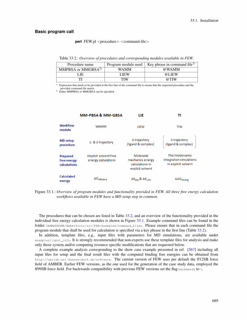
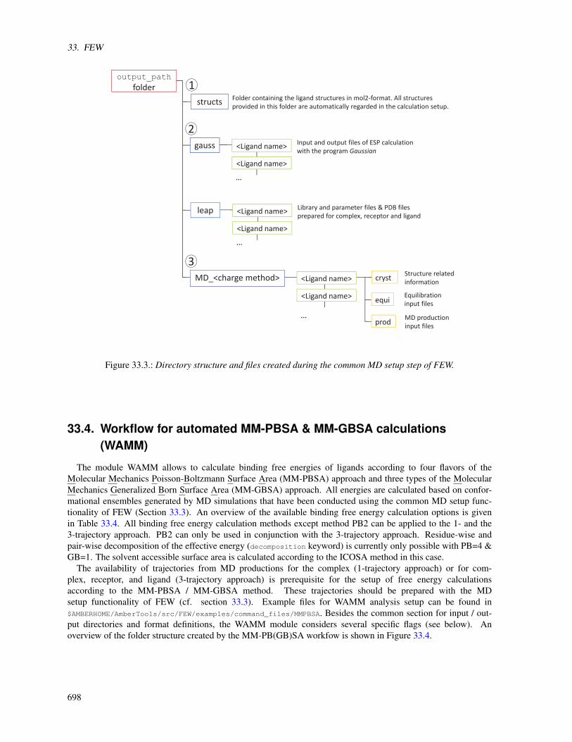
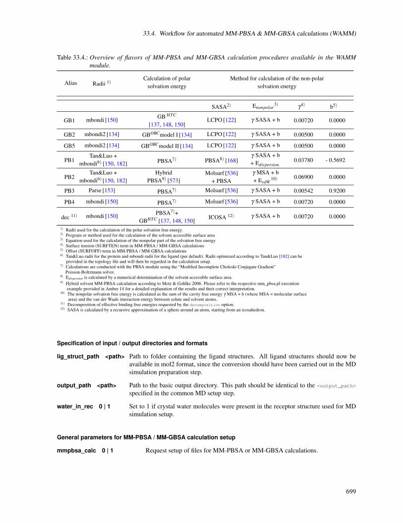
33. FEW 68833.1. Installation . . . . . . . . . . . . . . . . . . . . . . . . . . . . . . . . . . . . . . . . . . . . . . 68833.2. Overview of workflow steps and minimal input . . . . . . . . . . . . . . . . . . . . . . . . . . . 69033.3. Common setup of molecular dynamics simulations . . . . . . . . . . . . . . . . . . . . . . . . . 69233.4. Workflow for automated MM-PBSA & MM-GBSA calculations (WAMM) . . . . . . . . . . . . 69833.5. Linear interaction energy workflow (LIEW) . . . . . . . . . . . . . . . . . . . . . . . . . . . . . 70733.6. Thermodynamic integration workflow (TIW) . . . . . . . . . . . . . . . . . . . . . . . . . . . . 711
34. XtalAnalyze 71934.1. XtalAnalyze.sh . . . . . . . . . . . . . . . . . . . . . . . . . . . . . . . . . . . . . . . . . . . . 71934.2. XtalPlot.sh . . . . . . . . . . . . . . . . . . . . . . . . . . . . . . . . . . . . . . . . . . . . . . 72134.3. md2map.sh . . . . . . . . . . . . . . . . . . . . . . . . . . . . . . . . . . . . . . . . . . . . . . 722
35. SAXS 72435.1. Introduction and theory . . . . . . . . . . . . . . . . . . . . . . . . . . . . . . . . . . . . . . . . 72435.2. Usage . . . . . . . . . . . . . . . . . . . . . . . . . . . . . . . . . . . . . . . . . . . . . . . . . 725
VI. NAB and AmberLite 728
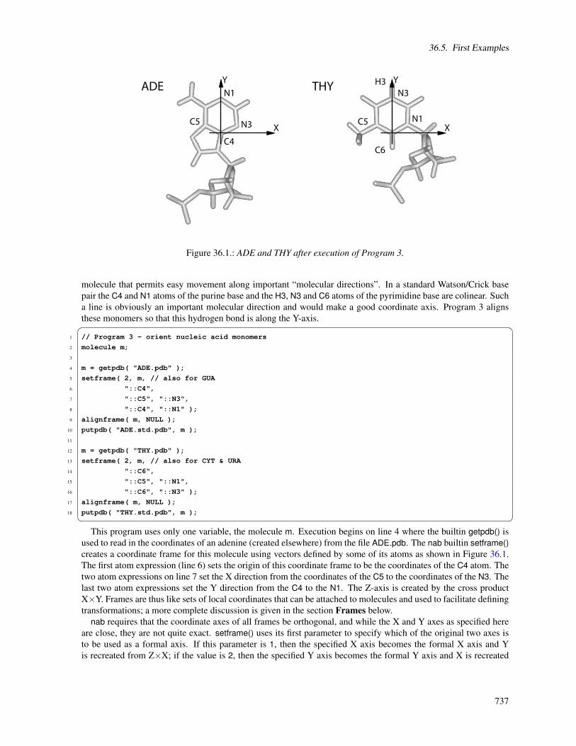
36. NAB: Introduction 73036.1. Background . . . . . . . . . . . . . . . . . . . . . . . . . . . . . . . . . . . . . . . . . . . . . . 73136.2. Methods for structure creation . . . . . . . . . . . . . . . . . . . . . . . . . . . . . . . . . . . . 73236.3. Compiling nab Programs . . . . . . . . . . . . . . . . . . . . . . . . . . . . . . . . . . . . . . . 73436.4. Parallel Execution . . . . . . . . . . . . . . . . . . . . . . . . . . . . . . . . . . . . . . . . . . . 73436.5. First Examples . . . . . . . . . . . . . . . . . . . . . . . . . . . . . . . . . . . . . . . . . . . . 73536.6. Molecules, Residues and Atoms . . . . . . . . . . . . . . . . . . . . . . . . . . . . . . . . . . . 73836.7. Creating Molecules . . . . . . . . . . . . . . . . . . . . . . . . . . . . . . . . . . . . . . . . . . 73836.8. Residues and Residue Libraries . . . . . . . . . . . . . . . . . . . . . . . . . . . . . . . . . . . . 73936.9. Atom Names and Atom Expressions . . . . . . . . . . . . . . . . . . . . . . . . . . . . . . . . . 74136.10.Looping over atoms in molecules . . . . . . . . . . . . . . . . . . . . . . . . . . . . . . . . . . . 74236.11.Points, Transformations and Frames . . . . . . . . . . . . . . . . . . . . . . . . . . . . . . . . . 74336.12.Creating Watson Crick duplexes . . . . . . . . . . . . . . . . . . . . . . . . . . . . . . . . . . . 744
37. NAB: Language Reference 75337.1. Language Elements . . . . . . . . . . . . . . . . . . . . . . . . . . . . . . . . . . . . . . . . . . 75337.2. Higher-level constructs . . . . . . . . . . . . . . . . . . . . . . . . . . . . . . . . . . . . . . . . 75537.3. Statements . . . . . . . . . . . . . . . . . . . . . . . . . . . . . . . . . . . . . . . . . . . . . . . 76137.4. Structures . . . . . . . . . . . . . . . . . . . . . . . . . . . . . . . . . . . . . . . . . . . . . . . 76337.5. Functions . . . . . . . . . . . . . . . . . . . . . . . . . . . . . . . . . . . . . . . . . . . . . . . 76437.6. Points and Vectors . . . . . . . . . . . . . . . . . . . . . . . . . . . . . . . . . . . . . . . . . . . 76537.7. String Functions . . . . . . . . . . . . . . . . . . . . . . . . . . . . . . . . . . . . . . . . . . . . 76637.8. Math Functions . . . . . . . . . . . . . . . . . . . . . . . . . . . . . . . . . . . . . . . . . . . . 76637.9. System Functions . . . . . . . . . . . . . . . . . . . . . . . . . . . . . . . . . . . . . . . . . . . 76737.10.I/O Functions . . . . . . . . . . . . . . . . . . . . . . . . . . . . . . . . . . . . . . . . . . . . . 76737.11.Molecule Creation Functions . . . . . . . . . . . . . . . . . . . . . . . . . . . . . . . . . . . . . 77037.12.Creating Biopoloymers . . . . . . . . . . . . . . . . . . . . . . . . . . . . . . . . . . . . . . . . 77137.13.Fiber Diffraction Duplexes in NAB . . . . . . . . . . . . . . . . . . . . . . . . . . . . . . . . . . 77137.14.Reduced Representation DNA Modeling Functions . . . . . . . . . . . . . . . . . . . . . . . . . 77237.15.Molecule I/O Functions . . . . . . . . . . . . . . . . . . . . . . . . . . . . . . . . . . . . . . . . 77337.16.Other Molecular Functions . . . . . . . . . . . . . . . . . . . . . . . . . . . . . . . . . . . . . . 77337.17.Debugging Functions . . . . . . . . . . . . . . . . . . . . . . . . . . . . . . . . . . . . . . . . . 77537.18.Time and date routines . . . . . . . . . . . . . . . . . . . . . . . . . . . . . . . . . . . . . . . . 776
10

CONTENTS
37.19.Computational resource consumption functions . . . . . . . . . . . . . . . . . . . . . . . . . . . 776
38. NAB: Rigid-Body Transformations 77738.1. Transformation Matrix Functions . . . . . . . . . . . . . . . . . . . . . . . . . . . . . . . . . . . 77738.2. Frame Functions . . . . . . . . . . . . . . . . . . . . . . . . . . . . . . . . . . . . . . . . . . . 77738.3. Functions for working with Atomic Coordinates . . . . . . . . . . . . . . . . . . . . . . . . . . . 77838.4. Symmetry Functions . . . . . . . . . . . . . . . . . . . . . . . . . . . . . . . . . . . . . . . . . 77838.5. Symmetry server programs . . . . . . . . . . . . . . . . . . . . . . . . . . . . . . . . . . . . . . 780
39. NAB: Distance Geometry 78439.1. Metric Matrix Distance Geometry . . . . . . . . . . . . . . . . . . . . . . . . . . . . . . . . . . 78439.2. Creating and manipulating bounds, embedding structures . . . . . . . . . . . . . . . . . . . . . . 78539.3. Distance geometry templates . . . . . . . . . . . . . . . . . . . . . . . . . . . . . . . . . . . . . 78939.4. Bounds databases . . . . . . . . . . . . . . . . . . . . . . . . . . . . . . . . . . . . . . . . . . . 791
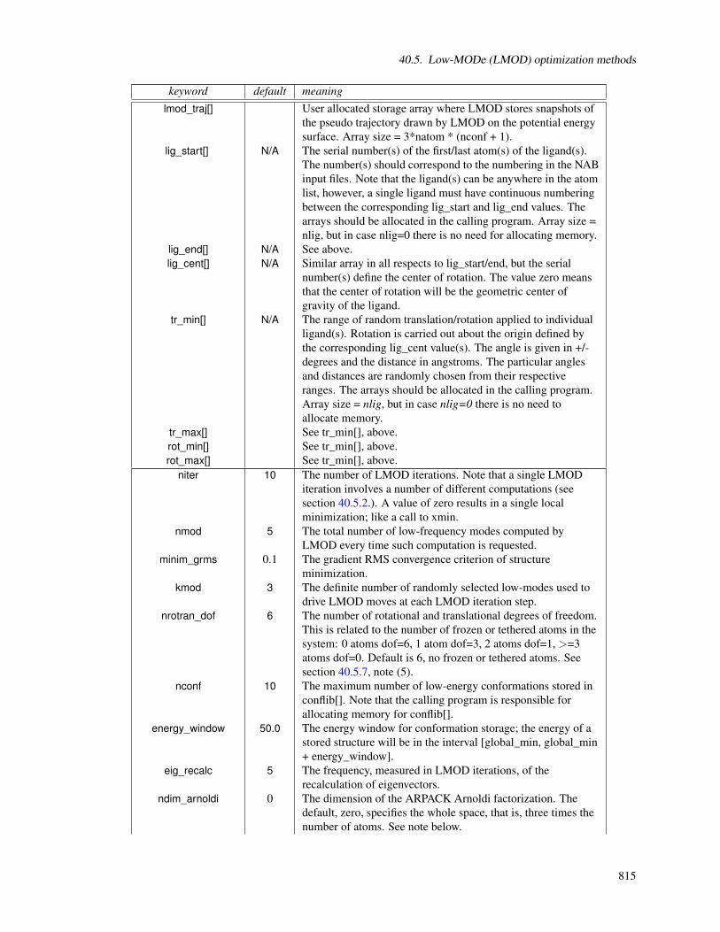
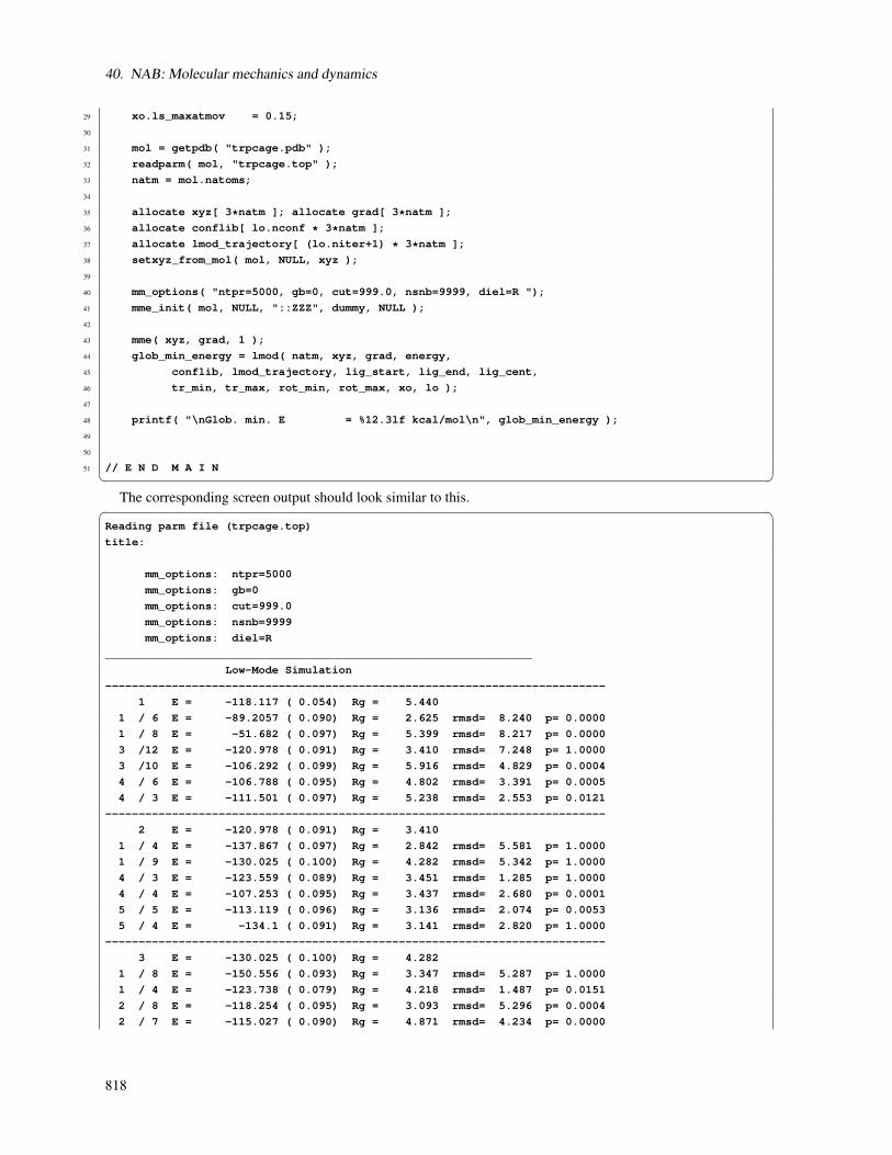
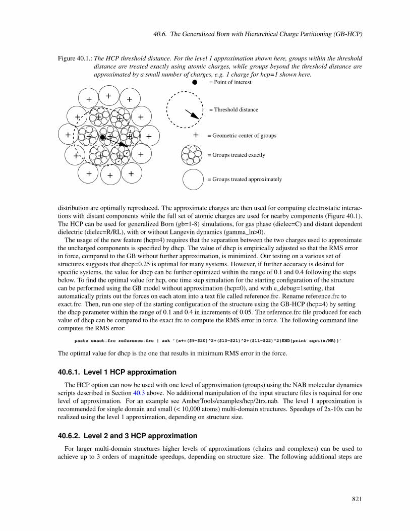
40. NAB: Molecular mechanics and dynamics 79340.1. Basic molecular mechanics routines . . . . . . . . . . . . . . . . . . . . . . . . . . . . . . . . . 79340.2. NetCDF read/write routines . . . . . . . . . . . . . . . . . . . . . . . . . . . . . . . . . . . . . . 80340.3. Typical calling sequences . . . . . . . . . . . . . . . . . . . . . . . . . . . . . . . . . . . . . . . 80640.4. Second derivatives and normal modes . . . . . . . . . . . . . . . . . . . . . . . . . . . . . . . . 80740.5. Low-MODe (LMOD) optimization methods . . . . . . . . . . . . . . . . . . . . . . . . . . . . . 80840.6. The Generalized Born with Hierarchical Charge Partitioning (GB-HCP) . . . . . . . . . . . . . . 820
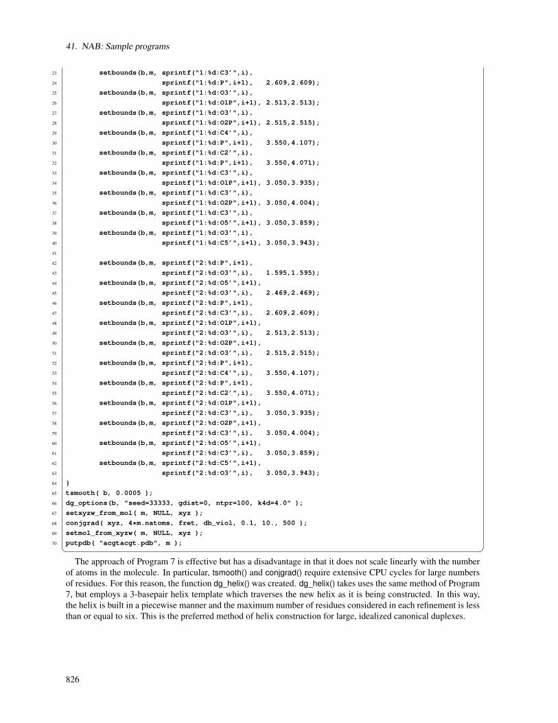
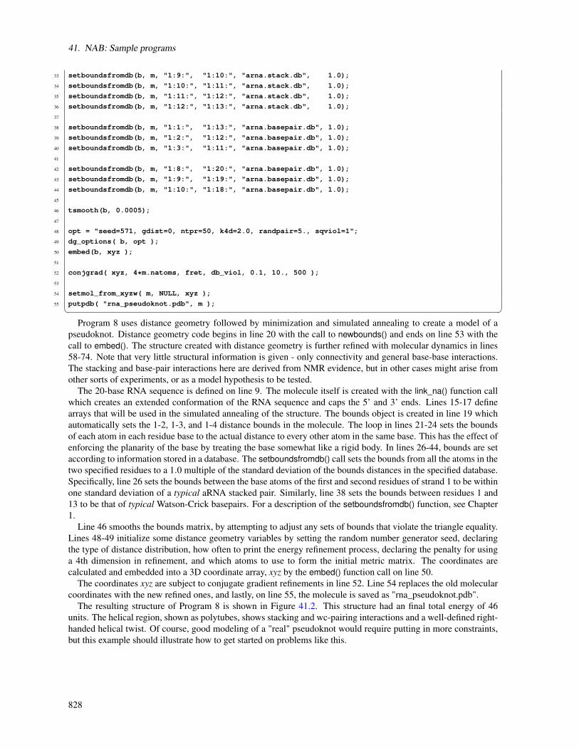
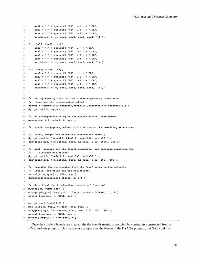
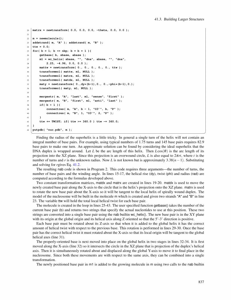
41. NAB: Sample programs 82341.1. Duplex Creation Functions . . . . . . . . . . . . . . . . . . . . . . . . . . . . . . . . . . . . . . 82341.2. nab and Distance Geometry . . . . . . . . . . . . . . . . . . . . . . . . . . . . . . . . . . . . . . 82441.3. Building Larger Structures . . . . . . . . . . . . . . . . . . . . . . . . . . . . . . . . . . . . . . 83241.4. Wrapping DNA Around a Path . . . . . . . . . . . . . . . . . . . . . . . . . . . . . . . . . . . . 83841.5. Other examples . . . . . . . . . . . . . . . . . . . . . . . . . . . . . . . . . . . . . . . . . . . . 844
42. amberlite: Some AmberTools-Based Utilities 84542.1. Introduction . . . . . . . . . . . . . . . . . . . . . . . . . . . . . . . . . . . . . . . . . . . . . . 84542.2. Coordinates and Parameter-Topology Files . . . . . . . . . . . . . . . . . . . . . . . . . . . . . . 84642.3. pytleap: Creating Coordinates and Parameter-
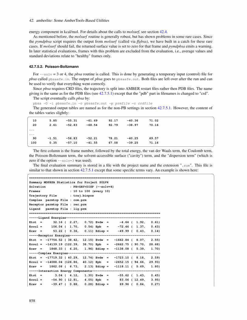
Topology Files . . . . . . . . . . . . . . . . . . . . . . . . . . . . . . . . . . . . . . . . . . . . 84842.4. Energy Checking Tool: ffgbsa . . . . . . . . . . . . . . . . . . . . . . . . . . . . . . . . . . . . 85142.5. Energy Minimizer: minab . . . . . . . . . . . . . . . . . . . . . . . . . . . . . . . . . . . . . . . 85142.6. Molecular Dynamics "Lite": mdnab . . . . . . . . . . . . . . . . . . . . . . . . . . . . . . . . . 85242.7. MM(GB)(PB)/SA Analysis Tool: pymdpbsa . . . . . . . . . . . . . . . . . . . . . . . . . . . . . 85342.8. Examples and Test Cases . . . . . . . . . . . . . . . . . . . . . . . . . . . . . . . . . . . . . . . 860
Bibliography 869
Index 912
11


Part I.
Introduction and Installation
13

1. Introduction
Amber is the collective name for a suite of programs that allow users to carry out molecular dynamics simu-lations, particularly on biomolecules. None of the individual programs carries this name, but the various partswork reasonably well together, and provide a powerful framework for many common calculations.[1, 2] The termAmber is also used to refer to the empirical force fields that are implemented here.[3, 4] It should be recognizedhowever, that the code and force field are separate: several other computer packages have implemented the Amberforce fields, and other force fields can be implemented with the Amber programs. Further, the force fields are inthe public domain, whereas the codes are distributed under a license agreement.
The Amber software suite is divided into two parts: AmberTools16, a collection of freely available programsmostly under the GPL license, and Amber16, which is centered around the pmemd simulation program, and whichcontinues to be licensed as before, under a more restrictive license. Amber16 represents a significant change fromthe most recent previous version, Amber14. (We have moved to numbering releases by the last two digits of thecalendar year, so there is no version 13 or 15.) Please see http://ambermd.org for an overview of the mostimportant changes.
AmberTools is a set of programs for biomolecular simulation and analysis. They are designed to work wellwith each other, and with the “regular” Amber suite of programs. You can perform many simulation tasks withAmberTools, and you can do more extensive simulations with the combination of AmberTools and Amber itself.Most components of AmberTools are released under the GNU General Public License (GPL). A few componentsare in the public domain or have other open-source licenses. See the README file for more information.
Everyone should read (or at least skim) this chapter. Even if you are an experienced Amber user, there may bethings you have missed, or new features, that will help. There are also tips and examples on the Amber Web pagesat http://ambermd.org. Although Amber may appear dauntingly complex at first, it has become easier to use overthe past few years, and overall is reasonably straightforward once you understand the basic architecture and optionchoices. In particular, we have worked hard on the tutorials to make them accessible to new users. Thousands ofpeople have learned to use Amber; don’t be easily discouraged.
If you want to learn more about basic biochemical simulation techniques, there are a variety of good books toconsult, ranging from introductory descriptions,[5–7] to standard works on liquid state simulation methods,[8–10]to multi-author compilations that cover many important aspects of biomolecular modelling.[11–15] Looking for"paradigm" papers that report simulations similar to ones you may want to undertake is also generally a good idea.If you are new to this field, Chapter 14 provides a basic introduction to force fields, along with details of how theparameters are encoded in Amber files.
1.1. Information flow in Amber
Understanding where to begin in AmberTools is primarily a problem of managing the flow of information inthis package — see Fig. 1.1. You first need to understand what information is needed by the simulation programs(sander, pmemd, mdgx or nab). You need to know where it comes from, and how it gets into the form that theseprograms require. This section is meant to orient the new user and is not a substitute for the individual programdocumentation.
Information that all the simulation programs need (see the circles in Fig. 1.1):
1. Cartesian coordinates for each atom in the system. These usually come from X-ray crystallography, NMRspectroscopy, or model-building. They should generally be in Protein Data Bank (PDB) format. The programLEaP provides a platform for carrying out many of these modeling tasks, but users may wish to considerother programs as well. Generally, editing of these files is needed, and the pdb4amber script can do some ofthis.
15

1. Introduction
pdb pdb4amber
antechamber,MCPB,LEaP
forcefieldinfo
prmtopprmcrd
par med.py
sander,nab, mdgx,
pmemd
NMR orXRAY info
mdininfo
mdout_analyzer,cpptraj
MMPBSA.py,amber lite,
FEW
Figure 1.1.: Basic information flow in Amber
2. Topology: Connectivity, atom names, atom types, residue names, and charges. This information comes fromthe database, which is found in the $AMBERHOME/dat/leap/lib directory, and is described in Chapter 3. Itcontains topology for the standard amino acids as well as N- and C-terminal charged amino acids, DNA,RNA, and common sugars and lipids. Topology information for other molecules (not found in the standarddatabase) is kept in user-generated “residue files”, which are generally created using antechamber.
3. Force field: Parameters for all of the bonds, angles, dihedrals, and atom types in the system. The standardparameters for several force fields are found in the $AMBERHOME/dat/leap/parm directory; see Chapter 3for more information. These files may be used “as is” for proteins and nucleic acids, or users may preparetheir own files that contain modifications to the standard force fields.
4. Once the topology and coordinate files (often called prmtop and prmcrd, but any legal file names can beused) are created, the parmed script can be used to examine and verify these, and to make modifications. Inparticular, the checkValidity action will flag many potential problems.
5. Commands: The user specifies the procedural options and state parameters desired. These are specified ininput files (named mdin by default) or in “driver” programs written in the NAB language.
1.1.1. Preparatory programs
LEaP is the primary program to create a new system in Amber, or to modify existing systems. It is available asthe command-line program tleap or the GUI xleap. It combines the functionality of prep, link, edit and parm
16
1.1. Information flow in Amber
from much earlier versions of Amber.
pdb4amber generally helps in preparing pdb-format files coming from other places (such as rcsb.org) to be com-patible with LEaP.
parmed provides a simple way to extract information about the parameters defined in a parameter-topology file. Itcan also be used to check that the parameter-topology file is valid for complex systems (see the checkValiditycommand), and it can also make simple modifications to this file very quickly.
antechamber is the main program to develop force fields for drug-like molecules or modified amino acids usingthe general Amber force field (GAFF). These can be used directly in LEaP, or can serve as a starting pointfor further parameter development.
MCPB.py provides a means to build, prototype, and validate MM models of metalloproteins and organometalliccompounds. It uses the bonded plus electrostatics model to expand existing pairwise additive force fields.It is a reimplementation of MCPB in Python, with a more efficient workflow and many modeling processesfrom previous versions incorporated automatically.
IPMach.py provides a tool to facilitate the parameterization of nonbonded models (12-6 LJ model and 12-6-4LJ-type model) for ions.
paramfit allows the generation of bonded force field parameters for any molecule by fitting to quantum data.
1.1.2. Simulation programs
sander (part of AmberTools) is the basic energy minimizer and molecular dynamics program. This programrelaxes the structure by iteratively moving the atoms down the energy gradient until a sufficiently low averagegradient is obtained. The molecular dynamics portion generates configurations of the system by integratingNewtonian equations of motion. MD will sample more configurational space than minimization, and willallow the structure to cross over small potential energy barriers. Configurations may be saved at regularintervals during the simulation for later analysis, and basic free energy calculations using thermodynamicintegration may be performed. More elaborate conformational searching and modeling MD studies can alsobe carried out using the sander module. This allows a variety of constraints to be added to the basic forcefield, and has been designed especially for the types of calculations involved in NMR, Xray or cryo-EMstructure refinement.
pmemd (part of Amber) is a version of sander that is optimized for speed and for parallel scaling; the pmemd.cudavariant runs on GPUs. The name stands for “Particle Mesh Ewald Molecular Dynamics,” but this code cannow also carry out generalized Born simulations. The input and output have only a few changes from sander.
mdgx is a molecular dynamics engine with functionality that mimics some of the features in sander and pmemd,but featuring simple C code and an atom sorting routine that simplifies the flow of information during forcecalculations. The principal purpose of mdgx is to provide a tool for redesign of the basic molecular dynamicsalgorithms and models, and for supporting new models for parameter development.
NAB (Nucleic Acid Builder) is a language that can be used to write programs to perform non-periodic simulations,most often using an implicit solvent force field.
1.1.3. Analysis programs
mdout_analyzer.py is a simple-to-run Python script that will provide summaries of information that is in theoutput files from sander or pmemd.
cpptraj is the main trajectory analysis utility (written in C++) for carrying out superpositions, extractions ofcoordinates, calculation of bond/angle/dihedral values, atomic positional fluctuations, correlation functions,analysis of hydrogen bonds, etc. It has many new features in version 16: see Chap. 29 for more information.
17

1. Introduction
pytraj is a Python wrapper for cpptraj. It is written to introduce more flexibility in data analysis by combiningwith Python’s rich echosystems (such as numpy, scipy, ipython-notebook ...).
pbsa is an analysis program for solvent-mediated energetics of biomolecules. It can be used to perform bothelectrostatic and non-electrostatic continuum solvation calculations with input coordinate files from molec-ular dynamics simulations and other sources (in the pqr format). It also supports visualization of solvent-mediated electrostatic potentials in various visualization programs.
MMPBSA.py is a python script that automates energy analysis of snapshots from a molecular dynamics simulationusing ideas generated from continuum solvent models. (There is also an older perl script, called mm_pbsa.pl,that has similar functionality.)
FEW (Free energy workflow) automates free energy calculations of protein-ligand binding using TI, MM/PBSA-type, or LIE calculations.
amberlite is small set of NAB programs and python scripts that implement a limited set of MD simulations andmm-pbsa (or mm-gbsa) analysis, aimed primarily at the analysis of protein-ligand interactions. These toolscan be useful in their own right, or as a good introduction to Amber and a starting point for more complexcalculations.
XtalAnalyze a set of utilities for analyzing crystal simulation trajectories. See Chapter 34 for more information.
1.2. List of programs
Amber is comprised of a large number of programs designed to aid you in your computational studies of chemicalsystems, and the number of released tools grows regularly. This section provides a list of the main programsincluded with AmberTools. Each program included in the suite is listed here with a very brief description of itsmain function along with which chapter in the manual a more thorough description can be found. Note: there aresome additional programs that are part of the MTK++ suite that are not listed here; see that documentation formore information.
AddToBox A program for adding solvent molecules to a crystal cell. See Subsection 16.3.
CartHess2FC.py A program to derive the force constants based on Cartesian Hessian matrix using Seminariomethod. SeeSubsection 15.8.2.5.
ChBox A program for changing the box dimensions of an Amber restart file. See Subsection 16.4.
CheckMD A program for automated checking of an MD simulation. Run the program without options for usagestatement.
IPMach.py A python program for facilitating the parameterization of the nonbonded models of ions. SeeSubsec-tion 15.8.2.2.
MCPB.py A python version of MCPB with optimized workflow. SeeSubsection 15.8.2.1.
MMPBSA.py A program to post-process trajectories to calculate binding free energies according to the MM/PBSAapproximation. See Chapter 31.
MTKppConstants Lists the constants used in MTK++. Run the program without arguments to get the full list.
OptC4.py optimizes the C4 terms in the metal-site-complex of a protein system. SeeSubsection 15.8.2.4
PdbSearcher.py a python version of Pdbsearcher, a program in MTK++. SeeSubsection 15.8.2.3
PropPDB A program for propagating a PDB structure. See Subsection 16.2
UnitCell A program for recreating a crystallographic unit cell from a PDB structure. See Subsection 16.1
18
1.2. List of programs
acdoctor A tool to diagnose what may be causing antechamber to fail. See Subsection 15.5.1
am1bcc A program called by antechamber to calculate AM1-BCC charges during ligand parametrization. Itcan be used as a standalone program, with the options printed when you enter the program name with noarguments. See Section 15.4
ambpdb A program to convert an Amber system (prmtop and inpcrd/restart) into a PDB, MOL2, or PQR file. SeeSection 28.1
ante-MMPBSA.py A program to create the necessary, self-consistent prmtop files for MMPBSA with a singlestarting topology file. See Subsection 31.2.2
antechamber A program for parametrizing ligands and other small molecules. See Chapter 15
atomtype A program called by antechamber to judge the atom types in an input structure. It can be used as astandalone program. If you provide no arguments, it prints out the usage statement. See Section 15.4
bondtype A program called by antechamber to judge what types of bonds exist in a given input structure. It canbe used as a standalone program. If you provide no arguments, it prints out the usage statement. See Section15.4
charmmlipid2amber.py A script that converts a PDB created with the CHARMM-GUI lipid builder into onerecognized by Amber and AmberTools programs. If you provide no arguments, it prints out the usagestatement.
cpinutil.py A program to create a constant pH input (CPin) file from a PDB file. If you provide no arguments,you get the usage statement.
cpptraj A versatile program for trajectory post-processing and data analysis. See Chapter 29
pytraj is a Python wrapper for cpptraj. See Section 30
cphstats A program that computes protonation state statistics from constant pH simulations. See Section 23.7
elsize A program that estimates the effective electrostatic size of a given input structure. See Section 4.2.1
espgen A program called by antechamber to generate ESP files during ligand or small molecule parametrization.If you provide no arguments, it prints out the usage statement.
espgen.py A python version of espgen. SeeSubsection 15.8.2.6.
ffgbsa A program that calculates MM/GBSA energies as part of the amberlite package.
FEW.pl A program to automate the workflow for free energy calculations. See Chapter 33
gbnsr6 A program to compute a surface-area-based Generalized Born solvation free energy. See Section 5
hcp_getpdb A program that adds necessary sections to a topology (prmtop) file so it can be used for the HCP GBapproximation. See Section 40.6
makeANG_RST A program to create angle restraints for use with sander’s nmropt=1 facility.
makeCHIR_RST A program to create chiral restraint file for use with sander’s nmropt=1 facility
makeDIP_RST.cyana A program to make restraints based on dipole information from CYANA for use withsander’s nmropt=1 facility
makeDIST_RST A program to make distance restraints for use with sander’s nmropt=1 facility
matextract Part of the symmetry definition programs, used to print matrices dumped to stdin to stdout. SeeSubsection 38.5.5
19

1. Introduction
matgen Generate symmetry-transformation matrices. Part of the symmetry definition programs. See Subsection38.5.1
matmerge Merges symmetry-transformation matrices into one matrix transformation matrix. Part of the symme-try definition programs. See Subsection 38.5.3
matmul Multiplies matrices. Part of the symmetry definition programs. See Subsection 38.5.4
mdgx An explicit solvent, PME molecular dynamics engine. See Chapter 27
mdnab Implicit solvent MD program written in NAB as part of Amberlite (Chapter 42)
mdout_analyzer.py A script that allows you to rapidly analyze and graph data from sander/pmemd output files.See Section 28
minab Implicit solvent minimization program written in NAB as part of Amberlite (Chapter 42)
mm_pbsa.pl Older perl script for performing MM/PBSA calculations. New users are encouraged to use MMPBSA.pyinstead.
mm_pbsa_statistics.pl Complementary script to mm_pbsa.pl to compute MM/PBSA statistics from a completedmm_pbsa calculation.
mm_pbsa_nabnmode Program for performing minimizations and normal mode analyses on biomolecules throughmm_pbsa.pl.
mmpbsa_py_energy A NAB program written to calculate energies for MMPBSA using either GB or PB solventmodels. It can be used as a standalone program that mimics the imin=5 functionality of sander, but it iscalled automatically inside MMPBSA. See MMPBSA mdin files as example input files for this program.Providing the –help or -h flags prints the usage message.
mmpbsa_py_nabnmode A NAB program written to calculate normal mode entropic contributions for MMPBSA.This can really only be used by MMPBSA.
molsurf A program that calculates a molecular surface area based on input PQR files and a probe radius. Providingno arguments prints the usage message.
nab Stands for Nucleic Acid Builder. NAB is really a compiler that provides a convenient molecular programminglanguage loosely based on C. See Chapter 36 and other related chapters.
new_crd_to_dyn Sets up a Tinker-style .DYN file from a coordinate file. This is part of the Tinker-to-Amberconversion program set.
new_to_old_crd Converts new Tinker-style coordinate files to old Amber-style coordinates. Part of the Tinker-to-Amber conversion program set.
nmode An outdated program to compute normal modes for biomolecules. You are encouraged to use NAB in-stead. See Section 40.1
paramfit Improves force field parameters by fitting to quantum data. See Chapter 11
parmcal Calculates parameters for given angles and bonds interactively. See Subsection 15.5.2
parmchk2 A program that analyzes an input force field library file (mol2 or amber prep), and extracts relevantparameters into an frcmod file. See Subsection 15.1.2
parmed A program for querying and manipulating prmtop files. See Section 14.2
pbsa A finite difference Poisson-Boltzmann solver. See Chapter 6
pdb4amber A program to prepares PDB files for use in leap. See Section 12.4
20

1.2. List of programs
pmemd A performance- and parallel-optimized dynamics engine implementing a subset of sander’s functionality
pmemd.cuda A GPU-accelerated version of pmemd
prepgen A program used as part of antechamber that generates an Amber prep file. Use no arguments to print theusage message. See Section 15.4
pymdpbsa A full analysis tool for MD(GB,PB)/SA computations. See Section 42.7
pytleap A user-friendly wrapper for simple leap and antechamber runs to prepare topology and coordinate filesfor Amber. See Section 42.3
reduce A program for adding or removing hydrogen atoms to a PDB. See Section 12.5
residuegen A program to automate the generation of an Amber residue template (i.e. Amber prep file). SeeSubsection 15.5.3
resp A program typically called by antechamber and R.E.D tools to perform a Restrained ElectroStatic Potentialcalculation for calculating partial atomic charges. Use no arguments to get the usage message
respgen A program called by antechamber to generate RESP input files. See Section 15.4
rism1d A 1D-RISM solver. See Section 7.4
rism3d.snglpnt A 3D-RISM solver for single point calculations. See Section 7.6
sander The main engine used for running molecular simulations with Amber. Originally an acronym standing forSimulated Annealing with Nmr-Derived Energy Restraints.
saxs_rism A program to compute small (wide) angle X-ray scattering curve from 3D-RISM output
saxs_md A program to compute small (wide) angle X-ray scattering curve from MD trajectories
softcore_setup.py A program to aid in softcore TI setup for sander. Use no arguments to get a usage message.
sqm Semiempirical (or Stand-alone) Quantum Mechanics solver. See Chapter 9
tinker_to_amber Converts a Tinker analout and parameter file into an Amber-compatible topology file.
tleap A script that calls teLeap with specific setup command-line arguments. See Chapter 13
transform Applies matrix transformations to a structure. Part of the symmetry definition programs. See Subsec-tion 38.5.6
tss_init A program to do some matrix stuff. See Section 38.5
tss_main A program to do some matrix stuff. See Section 38.5
tss_next A program to do some matrix stuff. See Section 38.5
ucpp A program to do some source code preprocessing. You should never actually use this program—it is usedby nab.
xaLeap A graphical program for creating Amber topology files. This program is called through the xleap script,so you should never actually invoke this program directly.
xleap A script that calls xaLeap with specific setup command-line arguments. See Chapter 13
xparmed A graphical front-end to ParmEd functionality (i.e., parameter file editing and querying). See Section14.2
21

2. Installation
This chapter gives an overview of how to install and test your distribution. The Amber web page (http://ambermd.org)has additional instructions and hints for various common operating systems. Look for the “Running Amber on ....”links. Once you have downloaded the distribution files, do the following:
1. First, extract the files in some location (we use /home/myname as an example here):
cd /home/myname
tar xvfj AmberTools16.tar.bz2 # (Note: extracts in an
# “amber16” directory)
tar xvfj Amber16.tar.bz2 # (only if you have licensed Amber 16!)
2. Next, set your AMBERHOME environment variable:
export AMBERHOME=/home/myname/amber16 # (for bash, zsh, ksh, etc.)
setenv AMBERHOME /home/myname/amber16 # (for csh, tcsh)
Be sure to change the “/home/myname” above to whatever directory is appropriate for your machine, and besure that you have write permissions in the directory tree you choose.
3. Next, you may need to install some compilers and other libraries. Details depend on what OS you have, andwhat is already installed. Package managers can greatly simplify this task. For example for Debian-basedLinux systems (such as Ubuntu), the following command should get you what you need:
sudo apt-get install csh flex gfortran g++ xorg-dev \
zlib1g-dev libbz2-dev patch python-tk python-matplotlib
See http://ambermd.org/linux_install.html for more information, and for requirements for other variants ofLinux, and for Macintosh OSX.
4. Now, in the AMBERHOME directory, run the configure script:
cd $AMBERHOME
./configure --help
will show you the options. Choose the compiler and flags you want; for most systems, the following shouldwork:
./configure gnu
This step will also check to see if there are any updates and bug fixes that have not been applied to yourinstallation, and will apply them (unless you ask it not to). If the configure step finds missing libraries, goback to Step 3. This step will also ask if you want to install a compatible Python executable for the Pythonprograms in Amber (including MMPBSA.py, MCPB.py, ParmEd, pysander, pytraj, pdb4amber, and the restof amberlite). Since Amber now requires Python 2.7 or later, along with numpy, scipy, and matplotlib toenable all of its functionality, configure now provides an option to download a compatible Python fromContinuum IO (via miniconda) installed in the Amber directory for use with Amber programs. See Section2.2 for more details. As long as your default Python has the required prerequisites installed, configure willsimply select that Python for use with Amber.
Do not choose any parallel options at this step! You will need to install the serial version first; options forparallel builds are described below at Step 8.
5. The configure step will create two resource files in the AMBERHOME directory: amber.sh and amber.csh.These sourceable scripts will set up your shell environment correctly for Amber:
23
2. Installation
source /home/myname/amber16/amber.sh # for bash, zsh, ksh, etc.
source /home/myname/amber16/amber.csh # for csh, tcsh
Of course, /home/myname/amber16 should be adjusted for your AMBERHOME. Adding these commandsto your login resource file (e.g., ~/.bashrc, ~/.cshrc, ~/.zshrc, etc.) will set up your environment every timeyou start a new shell. Note, this step is absolutely necessary to run any of the Python modules included withAmber.
6. Then,
make install
will compile the codes. If this step fails, try to read the error messages carefully to identify the problem.
7. This can be followed by
make test
which will run tests and will report successes or failures.
Where "possible FAILURE" messages are found, go to the indicated directory under $AMBERHOME/AmberTools/testor $AMBERHOME/test, and look at the "*.dif" files. Differences should involve round-off in the final digitprinted, or occasional messages that differ from machine to machine (see below for details). As with compi-lation, if you have trouble with individual tests, you may wish to comment out certain lines in the Makefiles(i.e., $AMBERHOME/AmberTools/test/Makefile or $AMBERHOME/test/Makefile), and/or go directly tothe test subdirectories to examine the inputs and outputs in detail. For convenience, all of the failure mes-sages and differences are collected in the $AMBERHOME/logs directory; you can quickly see from these ifthere is anything more than round-off errors.
The nature of molecular dynamics, is such that the course of the calculation is very dependent on the orderof arithmetical operations and the machine arithmetic implementation, i.e., the method used for round-off.Because each step of the calculation depends on the results of the previous step, the slightest differencewill eventually lead to a divergence in trajectories. As an initially identical dynamics run progresses ontwo different machines, the trajectories will eventually become completely uncorrelated. Neither of themare "wrong;" they are just exploring different regions of phase space. Hence, states at the end of longsimulations are not very useful for verifying correctness. Averages are meaningful, provided that normalstatistical fluctuations are taken into account. "Different machines" in this context means any difference infloating point hardware, word size, or rounding modes, as well as any differences in compilers or libraries.Differences in the order of arithmetic operations will affect round-off behavior; (a + b) + c is not necessarilythe same as a + (b + c). Different optimization levels will affect operation order, and may therefore affectthe course of the calculations.
All initial values reported as integers should be identical. The energies and temperatures on the first cycleshould be identical. The RMS and MAX gradients reported in sander are often more precision sensitivethan the energies, and may vary by 1 in the last figure on some machines. In minimization and dynamicscalculations, it is not unusual to see small divergences in behavior after as little as 100-200 cycles.
Note: If you have untarred the Amber16.tar.bz2 file, then steps 1-6 will install and test both AmberToolsand Amber; otherwise it will just install and test AmberTools. If you license Amber later, just come back andrepeat steps 1-6 again.
8. If you are new to Amber, you should look at the tutorials and this manual and become familiar with howthings work. If and when you wish to compile parallel (MPI) versions of Amber, do this:
cd $AMBERHOME
./configure -mpi <....other options....> <compiler-choice>
make install
# Note the value below may depend on your MPI implementation
export DO_PARALLEL=”mpirun -np 2”
make test
24

2.1. Uninstalling and cleaning
# Note, some tests, like the replica exchange tests, require more
# than 2 threads, so we suggest that you test with either 4 or 8
# threads as well
export DO_PARALLEL=”mpirun -np 8”
make test
This assumes that you have installed MPI and that mpicc and mpif90 are in your PATH. Some MPIinstallations are tuned to particular hardware (such as infiniband), and you should use those versions if youhave such hardware. Most people can use standard versions of either mpich or openmpi. To install one ofthese, use one of the simple scripts that we have prepared:
cd $AMBERHOME/AmberTools/src
./configure_mpich <compiler-choice> OR
./configure_openmpi <compiler-choice>
Follow the instructions of these scripts, then return to beginning of step 7.
Amber 16 brings with it an additional flag (-intelmpi) to enable use of the Intel® MPI Library. Use thisinstead of -mpi in step 8 and ensure that you have installed the Intel® MPI Library, and that mpiicc andmpiifort are in your PATH.
Some notes about the parallel programs in AmberTools:
1. The MPI version of nab is called mpinab, by analogy with mpicc or mpif90: mpinab is a compiler thatwill produce an MPI-enabled executable from source code written in the NAB language. Before compilingmpinab, be sure that you are familiar with the serial version of nab and that you really need a parallel version.If you have shared-memory nodes, the OpenMP version might be a better alternative. See Section 36.4 formore information. (Note that mpinab is primarily designed to write driver routines that call MPI versions ofthe energy functions; it is not set up to write your own, novel, parallel codes.)
2. The MPI version of MMPBSA.py is called MMPBSA.py.MPI, and requires the package mpi4py to run. If it isnot present in your Python standard library already, it will be built along with MMPBSA.py.MPI and placed inthe $AMBERHOME prefix. If you have problems with MMPBSA.py.MPI, see if you get the same problems withthe serial version, MMPBSA.py, to see if it is an issue with the parallel version or MMPBSA.py in general.Because we do not make or maintain the mpi4py source code, MMPBSA.py.MPI will not be available onplatforms on which mpi4py cannot be built.
3. NAB and Cpptraj can also be compiled using OpenMP:
./configure -openmp <....other options....> <compiler-choice>
make openmp
Note that the OpenMP version of NAB has the same name as the single-threaded version. See section 36.4for information on running the OpenMP version of NAB and section 29.1.6 for information on running theOpenMP version of Cpptraj.
4. See Section 19.6.5 for information about installing the GPU-accelerated versions of pmemd.
2.1. Uninstalling and cleaning
All of Amber and AmberTools is contained within the $AMBERHOME directory. So deleting this directory willcompletely remove Amber from your computer. However, there are cases when you may wish to remove some ofthe files and programs that were created when you compiled Amber; this section describes the Makefile rules thatare provided for those purposes.
make clean This command will remove all of the temporary object files that were created when you compiledAmber (these files usually reside in the same directory as the source code). This is necessary, for instance,when you intend to build a new variant of the Amber programs (such as building the OpenMP-parallelized
25

2. Installation
programs or the MPI-parallelized programs). This is done automatically by the configure script. The onlytime this would really be necessary is if you were modifying the compiler flags by editing the config.h fileby hand or setting the AMBERBUILDFLAGS environment variable. These are considered advanced options.
make distclean This command is a sledgehammer—it deletes all of the temporary object files, installed libraries,and programs, as well as several third-party libraries (but not things you might have installed separately,like MPI implementations via the configure_openmpi or configure_mpich scripts). The purpose of thiscommand is to return the source code tree to a pristine state, as though you just extracted a fresh copy ofthe source code. If you plan on changing the compiler that you use to build Amber, you should run thiscommand first.
Note that none of the above commands reverse any of the updates that you have already applied—they only impactfiles and programs that were created during the install process.
2.2. Python in Amber
Recent developments in Amber have increasingly added the Python programming language as the core languageof several of its components. In addition to standalone programs like MMPBSA.py, MCPB.py, and ParmEd, agrowing number of components also expose a substantial fraction of Amber functionality through Python APIs,like pysander, ParmEd, and pytraj.
Amber’s Python programs and libraries take advantage of the rich, mature, and robust scientific computingecosystem founded on the numpy numerical programming package. Standard dependencies for many AmberPython packages include numpy, scipy, matplotlib, and tkinter, just to name a few. As the Python language matures,modern tools begin to lose compatibility with older versions of Python. Many key components of Amber, beginningwith version 16, are compatible only with versions of Python 2.7 and later.
Since some Linux variants ship with versions of Python older than this, AmberTools includes a configure_pythonscript that will download and install a compliant Python version inside the Amber install directory in order to driveAmber’s Python components. If the standard configure process does not detect a Python that is both new enough,and has enough core components installed to run the bulk of Amber Python capabilities, you will be asked if youwant configure to download and install a version of Miniconda (shipped by Continuum IO) for you.
If you are not an experienced Python user, we recommend that you choose “yes” and allow AmberTools tocreate and manage the Python environment it needs for all of its tools. If you are an experienced Python user, andwould like to make use of the various AmberTools Python APIs, see the options for installing AmberTools Pythonpackages to the standard Python environments below.
This is a list of packages that AmberTools will install if user chose “yes”: python2.7, numpy, scipy, cython,ipython, notebook, matplotlib. The total downloaded file size is ~100 MB and the total installed size will be ~0.5GB. User can access Python via amber.python.
2.2.1. Picking your Python interpreter
By default, configure will attempt to use the standard python executable that it finds in the path (the one identifiedby the command “which python”). If this is not compliant with Amber’s basic prerequisites, you will be notifiedand asked if you want to install Miniconda. If so, AmberTools will download and install this version of Python 2.7(and will always look for that version first in future configure calls unless told to look elsewhere).
You can use the --with-python flag to configure (via --with-python /path/to/python) in order to specifya particular Python executable you wish to use with Amber. This flag overrides the checks for existing prerquisites,and should only be used if you know what you are doing.
2.2.2. Python package install location
By default, AmberTools attempts to install Python packages to $AMBERHOME/lib/pythonX.Y, where X.Y isthe version of Python was found (or assigned) by configure. If configure installed a version of Miniconda, this is
26

2.2. Python in Amber
$AMBERHOME/lib/python2.7. The amber.sh and amber.csh resource scripts then add this path to your PYTHON-PATH environment variable to ensure that the Python runtime can find these packages. In some cases, like withthe standard Phenix bindings, external programs may depend on the Python packages from Amber being installedto that location, so choosing one of the other options risks breaking third-party extensions. For somebody expe-rienced with using and developing Python, such problems will be easy to spot and fix. If you are unsure, you aresuggested to keep the default behavior.
In many cases, however, users may have sophisticated Python environments set up (through conda orvirtualenv, for instance) and would like Amber’s Python components to mesh more naturally in their Pythonenvironment than simply being dumped to $AMBERHOME/lib/pythonX.Y. For these use cases, the--python-install option was added to configure, which takes either user, local, or global as arguments. localis the default behavior. Selecting user installs all Python packages via the command
python setup.py install --user
which makes the packages automatically visible to the Python runtime, but does not require modifying anysystem-level directories that may require root access (however, it also will not work for any other user accounts).The global option will simply run
python setup.py install
and try to install all of the Amber modules and packages to the root level Python site-packages directory. Thiswill require root access if you are using the system Python (not recommended), but may not require any specialpermissions if using a local installation of Python, such as that from Anaconda or Miniconda.
2.2.3. Supported Python versions
Users are encouraged to use Python versions 2.7 and 3.4 (or greater) since those versions have been verifiedto work with all Python components of Amber (assuming other prerequisites, like numpy and/or scipy are met).Python 2.6 is known not to work with pytraj and ParmEd (and, by extension, any package that depends on ParmEd,like MMPBSA.py).
Different components of AmberTools support different versions of Python. For instance, as of AmberTools 16,ParmEd requires Python 2.7 or newer, while charmmlipidtoamber.py is compatible with Python 2.4. Some codes(like pytraj and ParmEd) work unchanged in both Python 2.7 and Python 3.x, while others need to be convertedusing 2to3 upon installation.
If users want to combine AmberTools (such as pysander, ParmEd) with 3rd party packages like phenix, Py-Rosetta, users need to use Python 2.7 version since those packages have not yet supported Python 3.x.
2.2.4. Amber’s Python environment and installing new components
If you said “yes” to allow configure to install Python from Miniconda, or you ran the configure_python scriptdirectly, Python is installed to $AMBERHOME/miniconda. Symbolic links to the main python, ipython, jupyterand conda executables are created in $AMBERHOME/bin and named amber.python, amber.ipython, amber.jupyter,and amber.conda, respectively. This is done to avoid potential collisions with other Python environments that maybe present.
The conda program is the Python package manager that is used to install new Python packages. So if you needto install a new package, you can use the amber.conda program to do so. For example, to install the pandaslibrary, use the command
amber.conda install pandas
You are referred to the Continuum IO documentation about Anaconda (and Miniconda) for further information.See https://www.continuum.io/documentation for more information.
27

2. Installation
2.3. Applying Updates
For most users, simply running the configure script and responding ‘yes’ to the update request will automaticallydownload and apply all patches. This section describes the main updating script responsible for managing updates.We suggest that you at least skim the first section on the basic usage—particularly the note about the --version
flag for if/when you ask for help on the mailing list.
2.3.1. Basic Usage
Updates to AmberTools and Amber are downloaded, applied, and managed automatically using the Pythonscript update_amber. This script works on every version of Python from Python 2.4 through the latest Python 3release. The configure script in $AMBERHOME automatically uses update_amber to search for available updates toAmberTools (and Amber when present) unless explicitly disabled with the --no-updates flag (which must be thefirst option to configure). If any are available, you will be asked if you want them downloaded and applied. Thisscript resides in $AMBERHOME and can be executed from anywhere (it will verify that AMBERHOME is set properly),but if moved from AMBERHOME, it will not work. There are 3 main operating modes, or actions, that you can performwith them:
• $AMBERHOME/update_amber --check-updates : This option will query the Amber website for any up-dates that have been posted that have not been applied to your installation. If you think you have found abug, this is helpful to try first before emailing with problems since your bug may have already been fixed.
• $AMBERHOME/update_amber --version : This option will return which patches have been applied to thecurrent tree so far. When emailing the Amber list with problems, it is important to have the output of thiscommand, since that lets us know exactly which updates have been applied.
• $AMBERHOME/update_amber --update : This option will go to the Amber website, download all updatesthat have not been applied to your installation, and apply them to the source code. Note that you will
have to recompile any affected code for the changes to take effect!
2.3.2. Advanced options
update_amber has additional functionality as well that allows more intimate control over the patching process.For a full list of options, use the --full-help command-line option. These are considered advanced options.
• $AMBERHOME/update_amber --download-patches : Only download patches, do not apply them
• $AMBERHOME/update_amber --apply-patch=<PATCH> : This will apply a third-party patch
• $AMBERHOME/update_amber --reverse-patch=<PATCH> : Reverses a third-party patch file that was ap-plied via the --apply-patch option (see above).
• $AMBERHOME/update_amber --show-applied-patches : Shows details about each patch that has beenapplied (including third-party patches)
• $AMBERHOME/update_amber --show-unapplied-patches : Shows details about each patch that has beendownloaded but not yet applied.
• $AMBERHOME/update_amber --remove-unapplied : Deletes all patches that have been downloaded butnot applied. This will force update_amber to download a fresh copy of that patch.
• $AMBERHOME/update_amber --update-to AmberTools/#,Amber/# : This command will apply all patchesnecessary to bring AmberTools up to a specific version and Amber up to a specific version. Note, no up-dates will ever be reversed using this command. You may specify only an AmberTools version or an Amberversion (or both, comma-delimited). No patches are applied to an omitted branch.
• $AMBERHOME/update_amber --revert-to AmberTools/#,Amber/# : This command does the same as--update-to described above, except it will only reverse patches, never apply them.
28

2.4. Contacting the developers
update_amber will also provide varying amounts of information about each patch based on the verbosity setting.The verbose level can be set with the --verbose flag and can be any integer between 0 and 4, inclusive. Thedefault verbosity level changes based on how many updates must be described. If only a small number of updatesneed be described, all details are printed out. The more updates that must be described, the less information isprinted. If you manually set a value on the command-line, it will override the default. These values are describedbelow (each level prints all information from the levels before plus additional information):
• 0: Print out only the name of the update file (no other information)
• 1: Also prints out the name of the program(s) that are affected
• 2: Also prints out the description of the update written by the author of that update.
• 3: Also prints the name of the person that authored the patch and the date it was created.
• 4: Also prints out the name of every file that is modified by the patch.
2.3.3. Internet Connection Settings
If update_amber ever needs to connect to the internet, it will check to see if http://ambermd.org can be contactedwithin 10 seconds. If not, it will report an error and quit. If your connection speed is particularly slow, you canlengthen this timeout via the --timeout command-line flag (where the time is given in seconds).
Proxies By default, update_amber will attempt to contact the internet through the same mechanism asprograms like wget and curl. For users that connect to the internet through a proxy server, you can either set thehttp_proxy environment variable yourself (in which case you can ignore the rest of the advice about proxieshere), or you can configure update_amber to connect to the internet through a proxy. To set up update_amber toconnect to the internet through a proxy, use the following command:
$AMBERHOME/update_amber --proxy=<PROXY_ADDRESS>
You can often find your proxy address from your IT department or the preferences in your favorite (configured)web browser that you use to surf the web. If your proxy is authenticated, you will also need to set up a user:
$AMBERHOME/update_amber --proxy-user=<USERNAME>
If you have set up a user name to connect to your proxy, then you will be asked for your proxy password the firsttime update_amber attempts to utilize an online resource. (For security, your password is never stored, and willneed to be retyped every time update_amber runs).
You can clear all proxy information using the --delete-proxy command-line flag—this is really only necessaryif you no longer need to connect through any proxy, since each time you configure a particular proxy user or serverit overwrites whatever was set before.
Mirrors If you would like to download Amber patches from another website or even a folder on a local filesystem,you can use the --amber-updates and --ambertools-updates command-line flags to specify a particular webaddress (must start with http://) or a local folder (use an absolute path). You can use the --reset-remotes
command-line flag to erase these settings and return to the default Amber locations on http://ambermd.org.If you set up online mirrors and never plan on connecting directly to http://ambermd.org, you can change
the web address that update_amber attempts to connect to when it verifies an internet connection using the--internet-check command-line option.
2.4. Contacting the developers
Please send suggestions and questions to [email protected]. You need to be subscribed to post there; tosubscribe, go to http://lists.ambermd.org/mailman/listinfo/amber. You can unsubscribe from this mailing list onthe same site.
29


Part II.
Amber force fields
31


3. Molecular mechanics force fields
Amber is designed to work with several simple types of force fields, although it is most commonly used withparametrizations developed by Peter Kollman and his co-workers and “descendents”. The traditional parametriza-tion uses fixed partial charges, centered on atoms. Less commonly used modifications add polarizable dipoles toatoms, so that the charge description depends upon the environment; such potentials are called “polarizable” or“non-additive”. An alternative is to use force fields originally developed for the CHARMM or tinker (AMOEBA)codes; these require a different setup procedure, which is described in Sections 14.2.2.8 (for CHARMM) andChapter 17 (for AMOEBA). Chapter 14 provides a basic introduction to force fields, along with details of how theparameters are encoded in Amber files.
In previous versions of AmberTools, we including “combined” leaprc files (such as leaprc.ff14SB) that loaded,protein, nucleic acid and water models that worked well together. This was convenient for most users, but tendedto obfuscate the important issue of deciding which force fields to use. Since various choices make good sense, andwe have implemented a new scheme for users to specify the force fields they wish to use. Depending on whatcomponents are in your system, you may need to specify:'
&
$
%
• a protein force field (recommended choice is ff14SB)
• a DNA force field (recommended choice is OL15)
• an RNA force field (recommended choice is OL3)
• a carbohydrate force field (recommended choice is GLYCAM_06j)
• a lipid force field (recommended choice is lipid14)
• a water model with associated atomic ions (more variable, but the most common choice is still tip3p); otherpopular choices are spc/e, tip4pew, and OPC. Not needed if you are using an implicit solvent model.
• a general force field, for organic molecules like ligands (recommended choice is gaff2)
• other components (such as modified amino acids or nucleotides, other ions), as needed
Notes:
1. You have to be careful if you try to adopt a “mix and match” strategy for different components. The recom-mended choices are designed to work well together, and have been fairly extensively tested. Use of othercombinations requires a deeper knowledge of the nature and origin of force fields; see below and consult theoriginal papers for more information. If you wish to combine proteins with nucleic acids, only the recom-mended combination above (or one where leaprc.DNA.OL15 is replaced with leaprc.DNA.bsc1) is allowed.
2. In general, your input file to leap will begin with several commands to source the relevant leaprc files. Forexample the following preamble would allow you to include proteins, DNA, lipids, general components,water, and atomic ions like Na+ or Cl-, using the current recommended force fields: source leaprc.protein.ff14SB
source leaprc.DNA.OL15
source leaprc.lipid14
source leaprc.tip3p
source leaprc.gaff2
33

3. Molecular mechanics force fields
3. There are some leaprc files for older force fields in the $AMBERHOME/dat/leap/cmd/oldff directory. We nolonger recommend these combinations, but we recognize that there may be reasons to use them, especiallyfor comparisons to older simulations. See Section 3.9 for more information.
4. In particular, the leaprc.ff14SB file, in the oldff/ directory, is identical to the file of the same name in Amber-Tools15. In spite of its name, it is a “combined” file, with protein, DNA, RNA and water elements. This filemight be of particular interest if you want to make sure that systems created the “new” way (with the leaprcfiles outlined above) are consistent with those using the older, “combined” method.
3.1. Proteins
In addition to the recommended file, leaprc.protein.ff14SB, there are a variety of alternatives for proteins; theseare described in the following sections.
3.1.1. The ff14SB force field leaprc.protein.ff14SB This will load the files listed below
parm10.dat ff10 force field parameters
frcmod.ff14SB ff14SB modifications to parm10.dat
amino12.lib topologies and charges for amino acids
amino12nt.lib same, for N-terminal amino acids
amino12ct.lib same, for C-terminal amino acids
leaprc.protein.ff14SBonly This is the same as leaprc.protein.ff14SB, but will additionally load:
frcmod.ff99SB14 ff99SB backbone parameters with ff14SB atom types ff14SB [16]is a continuing evolution of the ff99SB force field, primarily developed in the Simmerling group
at Stony Brook University.[17] Several groups had noticed that the older ff94 and ff99 parameter sets did notprovide a good energy balance between helical and extended regions of peptide and protein backbones. Anotherproblem is that many of the ff94 variants had incorrect treatment of glycine backbone parameters. ff99SB improvedthis behavior, presenting a careful reparametrization of the backbone torsion terms in ff99 and achieves muchbetter balance of four basic secondary structure elements (PP II, β , αL, and αR). A detailed explanation of theparametrization as well as an extensive comparison with many other variants of fixed-charge Amber force fieldsis given in the reference above. Briefly, dihedral term parameters were obtained through fitting the energies ofmultiple conformations of glycine and alanine tetrapeptides to high-level ab initio QM calculations. We haveshown that this force field provides much improved proportions of helical versus extended structures. In addition, itcorrected the glycine sampling and should also perform well for β -turn structures, two things which were especiallyproblematic with most previous Amber force field variants.
Since 2006, a number of limitations of the ff99SB parameter sets became evident, and a new round of parameteroptimization was undertaken. The changes mainly involve torsional parameters for the backbone and side chains.For backbones, experimental scalar coupling data for small solvated peptides became available [18] against whichff99SB was compared.[19] As ff99SB backbone dihedrals were fit based on gas-phase quantum data, we felt thatslight empirical adjustments were worth pursuing. This was done to improve agreement with scalar coupling data,and we observed that this also improved stabilities of helical peptides.
The side chain dihedral parameters of ff99SB were the same as those of ff99. Residues such as isoleucine,leucine, aspartate, and asparagine (cf. ff99SB-ILDN) sample conformations different from those indicated by ex-periments. We therefore calibrated the dihedral corrections of the amino acid side chains against ab initio quantummechanical energy surfaces. As ff14SB is an additive model, a key objective was to minimize dependence offf14SB side chain parameters on particular backbone conformations. Therefore, side chain corrections were raisedagainst potential energy surfaces including multiple backbone conformations. Moreover, the method of generat-ing fitting data was adjusted to minimize backbone-dependence, including restraint of all backbone dihedrals andre-optimization of bonds and angles with each model. Whereas ff12SB also included restraints on all side chain di-hedrals, restraint of one dihedral per side chain bond in ff14SB was found to further reduce backbone-dependence.
34
3.1. Proteins
Together with new corrections for the backbone and the four amino acids addressed in ff99SB-ILDN, this workoffers updated side chain dihedral corrections for lysine, arginine, glutamate, glutamine, methionine, serine, thre-onine, valine, tryptophan, cysteine, phenylalanine, tyrosine, and histidine. ff14SB enhances reproduction of exper-imentally indicated geometries over ff99SB. See Ref. [16] for futher details.
ff14SBonlysc, where sc stands for side chains, includes ff99SB backbone parameters with updated side chainparameters that were derived from ab initio quantum mechanics calculations (as were the ff99SB backbone cor-rections). This model is slightly different from ff14SB, which includes the ff14SBonlysc parameters as well as asmall empirical correction to backbone parameters that was designed to improve agreement between NMR dataand simulations in TIP3P water for short peptides. We are currently exploring whether this empirical correctionalso improves simulations in other water models, such as the GBneck2 (igb=8) model. [20] Currently, it appearsthat igb=8 may work best with the fully quantum mechanics-based dihedral parameters included in ff14SBonlysc.Simulations performed in explicit water most likely benefit from the empirical corrections included in ff14SB.
3.1.2. The ff15ipq protein force field leaprc.protein.ff15ipq This will load the files listed below
parm15ipq_10.3.dat force field parameters
amino15ipq_10.0.lib topologies and charges for amino acids
aminont15_ipq10.0.lib same, for N-terminal amino acids
aminoct15ipq_10.0.lib same, for C-terminal amino acids ff15ipq continues the development begun with the ff14ipq force field [21, 22], but offers new, we hope better,
parameter choices, data fitting, and validation. The physical assumptions behind the model are the same, butproblems with ff14ipq, most generally the "stickiness" of polar groups in simulations, led to sweeping param-eter changes. The pair-specific Lennard-Jones terms in ff14ipq were the problem, introducing an imbalance ofprotein:water and protein:protein interactions. They have been replaced by modified polar hydrogen radii anda consistent Lorentz-Berthlot combining rule as found in other Amber force fields. As a consequence, the entirecharge set has changed, albeit slightly, and the the torsion parameters have been expanded and rederived. To furtherimprove the internal potential energy surface, refitted angle parameters are included for the protein backbone. Thenew version comprises nearly 1,200 unique parameters, and ff14ipq is archived (use oldff/leaprc.ff14ipq) forbackwards compatibility and comparisons.
The extended IPolQ charge derivation anticipates a workflow in which the final model must have charges roughlyconsistent with the polarization molecules experience in water, but also new torsion parameters which are oftenderived with quantum calculations of the system in vacuum. In the extended methodology, two sets of chargesare fitted: one for the systems in vacuum, the other for systems in the condensed phase. The original IPolQmethod [21] derives the appropriate condensed phase charges by fitting to the average electrostatic potential ofpolarized and unpolarized molecules, a process that harkens to linear response theory and implicitly accounts forthe energetic cost of polarizing the system away from is gas phase equilibrium. The extended scheme draws onthe vacuum phase electrostatic data a second time to make an alternative set of charges appropriate to describe thevacuum potential energy surface–the IPolQ charges themselves are, in fact, re-expressed as a perturbation of thisgas phase charge set. Both sets of charges are derived in the same linear least squares fitting problem, with restraintequations weakly coupling the corresponding charges together. This creates charge sets for each phase related bya minimal perturbation, which can be assumed to be the effective, average polarization of the molecules whenthey enter solution. The charge set appropriate to the vacuum phase is then used when fitting torsion potentialsto vacuum phase quantum mechanical energies, and the torsion potentials are transferred directly for use with thecondensed-phase charge set in actual simulations, following the earlier assumption that the effective polarizationof the molecules, and thereby any energetic consequences of entering the condensed phase, are captured in thecharge perturbation.
All parameter optimization in ff15ipq, like its predecessor ff14ipq, is iterative: a generational learning schemewhereby the results of previous simulations and force field manipulations are submitted to quantum single pointenergy calculations and then added to the training data. As with ff14ipq, charges and gas-phase conformationalenergies are all taken at the MP2/cc-pVTZ level; ff15ipq takes the ff14ipq conformational energies as its startingpoint and expands the space nearly four-fold. We find that this crude form of machine learning is a good substitute
35

3. Molecular mechanics force fields
for human intervention. As with ff14ipq, the iterative process led to an evolution in simulation performance overa variety of systems. We utilized these benchmarks to determine when the parameter set was ready for generalrelease.
The new ff15ipq model was derived with the SPC/E-b water model of Takemura and Kitao [23]. Returning tothree-point water models improves performance of most Amber protein simulations on GPUs by about 30% dueto the reduction in the overall number of particles; a smaller improvement can be seen on CPUs. While SPC/E-bis the recommended water model, the solvent reaction field potential observed in our IPolQ studies is consistentacross three- and even some four-point waters: combinations of ff15ipq with TIP3P, the original SPC/E, and otherwater models are reasonable to try. One issue that may arise in some circumstances is the compatibility of the watermodel with ion parameters: we have set ff15ipq to reference ion parameters appropriate for the nearest water modelavailable, SPC/E. However, for highly charged or dense ionic solutions this combination may be sub-optimal. Withrespect to compatibility with other macromolecular force fields such as sugars, lipids, or nucleic acids, we notethat while the charge set is novel, the MP2/cc-pVTZ solution-phase IPolQ charges [21] are in fact quite similar tothe Cornell charges derived at the HF/6-31G* level [24]. This result may support the long lifespan of that chargeset, and makes it likely that ff15ipq will be compatible with other force fields designed at the common HF/6-31G*level.
ff15ipq has been validated on a larger number of test systems than its predecessor, and for much longer timescales.Multiple alpha-helical and beta-sheet peptides have been tested at a variety of temperatures, and numerous smallproteins (the largest including lysozyme and the p53/MDM2 complex) have been simulated for timescales rangingfrom 4 to 10 microseconds, displaying excellent stability and also instability in cases where loops of the proteinsor isolated peptides are known to be disordered. Various teething problems in the ff14ipq force field were solvedby improvements to the data set or the fitting protocol itself, so we are increasingly confident that ff15ipq andfuture products of the IPolQ workflow will be reliable straight out of the automated parameter development phase.The entire data set and mdgx input file for deriving the torsion and angle parameters of ff15ipq will be released assupporting information in the upcoming publication on the force field. In the future we hope to build on the lineageof ff-ipq protein models to include other important areas of biological chemistry.
3.1.3. The fb15 (“force balance”) protein force field leaprc.protein.fb15 This will load the files listed below
frcmod.fb15 force field parameters
frcmod.tip3pfb parameters for the force balance 3-point model
all_aminofb15.lib topologies and charges for amino acids
all_aminontfb15.lib same, for N-terminal amino acids
all_aminoctfb15.lib same, for C-terminal amino acids The files can be used for protein-water simulations using the “force-balance” approach described in Ref. [25].There is also a 4-point water model available, as described in section 3.5. For alkali and halide ions, the Joung-Cheatham parameters for TIP3P (or TIP4PEW) are recommended; see Section 3.6.
3.1.4. The Duan et al. (2003) force field leaprc.protein.ff03.r1 loads the following files:
frcmod.ff03 For proteins: changes to parm99.dat, primarily in the
phi and psi torsions.
all_amino03.in Charges and atom types for proteins
all_aminont03.in For N-terminal amino acids
all_aminoct03.in For C-terminal amino acids The ff03 force field [26, 27] is a modified version of ff99 (described below). The main changes are that charges
are now derived from quantum calculations that use a continuum dielectric to mimic solvent polarization, and thatthe φ and ψ backbone torsions for proteins are modified, with the effect of decreasing the preference for helicalconfigurations. The changes are just for proteins; nucleic acid parameters are the same as in ff99.
36
3.2. Nucleic acids
The original model used the old (ff94) charge scheme for N- and C-terminal amino acids. This was what wasdistributed with Amber 9, and can still be activated by using oldff/leaprc.ff03. More recently, new libraries for theterminal amino acids have been constructed, using the same charge scheme as for the rest of the force field. Thisnewer version (which is recommended for all new simulations) is accessed by using leaprc.protein.ff03.r1.
3.1.5. The Yang et al. (2003) united-atom force field frcmod.ff03ua For proteins: changes to parm99.dat, primarily in the
introduction of new united-atom carbon types and new
side chain torsions.
uni_amino03.in Amino acid input for building database
uni_aminont03.in NH3+ amino acid input for building database.
uni_aminoct03.in COO- amino acid input for building database. The ff03ua force field [28] is the united-atom counterpart of ff03. This force field uses the same charging scheme
as ff03. In this force field, the aliphatic hydrogen atoms on all amino acid side-chains are united to their corre-sponding carbon atoms. The aliphatic hydrogen atoms on all alpha carbon atoms are still represented explicitly tominimize the impact of the united-atom approximation on protein backbone conformations. In addition, aromatichydrogens are also explicitly represented. Van der Waals parameters of the united carbon atoms are refitted basedon solvation free energy calculations. Due to the use of an all-atom protein backbone, the φ and ψ backbonetorsions from ff03 are left unchanged. The sidechain torsions involving united carbon atoms are all refitted. In thisparameter set, nucleic acid parameters are still in all atom and kept the same as in ff99.
3.2. Nucleic acids
As with proteins, many features of the current force fields, including partial atomic charges, Lennard-Jonesparameters, and most bond and angle terms, date back to force fields developed in the 1990’s, and overviews ofthis work are available.[29, 30] The next breakthroughs in the Amber nucleic acid force field development camefrom observations from relatively longer simulations on the 50-100 ns time scale in the early 2000’s.[31, 32] Thesesimulations found systematic over-population of γ = trans backbone geometries in nucleic acids. High level QMcalculations were performed on models of sugars and phosphates, specifically a sugar-phosphate model[33] anda sugar-phosphate-sugar model,[34] which ultimately led to the ff99-bsc0 parameterization.[33] For simulationof canonical DNA and RNA structures, the ff99-bsc0 parameterization has proven rather successful. For non-canonical structures, particular those with loops or bulges, or χ flips, some anomalies have been noted. WithRNA, incorrect loop geometries, backbone sub-state populations and sugar pucker populations were observed inlonger simulations. In addition to not being able to always maintain south puckers where found in RNA structures,multiple groups noticed a tendency for the RNA backbone to shift, putting χ into the high-anti region which leadsto an opening of the duplex structure into a ladder-like configuration. Again, QM methods at various levels wereemployed to improve the χ distribution using relevant model systems. The most tested χ modifications are the“OL” modifications used in ff14SB.[35, 36] An alternative available with Amber is the Yildirim χ modifications(and also related modifications called TOR which alter ε/ζ as well)[37–39], and a systematic assessment andvalidation of these newer χ modifications is underway on a large series of RNA tetraloop structures. Note thatsmall changes to a particular dihedral may lead to alteration in properties of related dihedrals, and may haveunintended consequences. For example, the ff99-bsc0 modifications tend to lock RNA sugar puckers mainly in thenorth, even with nucleotides in particular sequence contexts that prefer southern conformations. Moreover, the χ
modifications tend to further destabilize γ = trans. This suggests that to reliably improve the nucleic acid dihedrals,a more systematic approach across many dihedrals with simultaneous fitting may be more appropriate. Moreover,we no longer fully support the idea that parameters are transferable between DNA and RNA, or between purinesand pyrimidines. For example, the ff99-OL modifications (with or without ff99-bsc0) improve the modeling ofRNA, but lead to issues with DNA, most notably with quadruplex structures. Therefore recent work has focusedon separate χ modifications for DNA.[40]
A new set of parameters for the ε/ζ dihedral[41] and for the β dihedral[42] torsion for DNA have been de-veloped using QM methods that include the solvation effects implicitly. This set of parameters have been tested
37

3. Molecular mechanics force fields
Name Modification Notesff94 Original force field file Obsoleteff98 Modified charge set Obsoleteff99 Updated charge set Foundation for all current ff’sbsc0 Barcelona α/γ backbone modification [33]
χOL3 χmodification tuned for RNA [35, 36]ε/ζ OL1 ε/ζ modification for DNA improvement for DNA, no effects for RNA [41]
χ OL4 χ modification tuned for DNA [40]β OL1 β dihedral modification tuned for DNA improvement for DNA, no effects for RNA[42]bsc1 Major update to bsc0 [43]
Table 3.1.: Force field name and modifications for simulating nucleic acids.
Desired Behavior Source these files NotesRNA
ff99OL3 leaprc.RNA.OL3 parmbsc0 α/γ [33] + χOL3 [36] to ff99ff99χ + bsc0 leaprc.RNA.YIL parmbsc0 α/γ [33]+ Yildirim [37]χ mods to ff99.
ff99bsc0 oldff/leaprc.ff99bsc0 Contains parmbsc0 α/γ mods[33] to ff99.Modified nucleotides leaprc.modrna08 parameters for modified nucleosides [45]
DNAOL15 leaprc.DNA.OL15 Contains ε/ζOL1[41], χOL4[40] and βOL1[42] mods to ff14.bsc1 leaprc.DNA.bsc1 Contains parmbsc1 mods [43] to parmbsc0.
Table 3.2.: How to specify nucelic acid force fields in LEaP; recommended variants are in italics.
with several double-stranded DNA systems including the Dickerson-Drew dodecamer, A-tracs, CG-rich duplexes,Z-DNA and G-quadruplexes. These modifications increase the population of BII substate by stabilizing the ε/ζ
= g-/t state and renders higher values for the helical twist in the tested systems. In combination with the χ mod-ification for DNA (χOL4, [40]), the force field generates structures that suggest a better agreement with NMRdata. The reader should pay careful attention to the use of the χ modifications, since the naming convention of theauthors is the same for RNA and DNA.
The combination of the three dihedral updates (ε/ζ OL1+χOL4+βOL1) are now termed OL15 which are avail-able sourcing the file leaprc.nucleic.OL15. More details about the OL15 force field development and test cases isavailable in http://fch.upol.cz/ff_ol/.
In a parallel effort, the group at the Barcelona Supercomputing Center have updated the well-known bsc0 mod-ification, now termed bsc1.[43] This updated version of the bsc0 modification has also been developed usingimplicit solvation model and rigorous QM methodology. As with the OL15 variant, the updated bsc1 force fieldincreases the helical twist and yields double stranded DNA structures that are in better agreement with experimen-tal structures. Testing of the bsc1 force field has been performed using more than 130 systems, including singleand double stranded DNA, hairpin structures, DNA-protein complexes, G-quadruplexes and more. This can beaccessed by sourcing leaprc.nuclic.bsc1; additional information about the bsc1 force field development and testcases is available in http://mmb.irbbarcelona.org/ParmBSC1/.
Details of the different modifications available for DNA are presented in Table 3.1.Considering the multiple small modifications available, it is very important to do extensive testing and bench-
marking of any simulations done with these variations. This is ongoing work from different research groupsinvolved in the simulation of nucleic acids. For DNA, we recommend the OL15 force field and for RNA, werecommend using a combination of ff99 + bsc0 + χOL3.
Regarding the performance of OL15 and bsc1 for DNA, preliminary testing comparing both force fields stronglysuggest that both variations perform in a similar way and are improvements over the previous commonly bsc0modification.[44] We refer the reader to the original articles of each force field to better understand the details andperformance between each variant.
38

3.3. Carbohydrates
Note: Nucleic acid residues use the new (version 3) PDB nomenclature: “DC” is used for deoxy-cytosine, and“C” for cytosine in RNA, etc. Earlier force fields (which are not recommended!) use “RC” for the RNA version.If you want a single, nucleoside, use “CN”, etc. For a single nucleotide, use the following command in LEaP:
cnuc = sequence OHE C3
and analogs for other bases. Note that this will construct a protonated 5’ phosphate group, which may not be whatyou want.
3.3. Carbohydrates
GLYCAM06 is a consistent and transferable parameter set for modeling carbohydrates,[46] and glycoconjugates.[47,48] The core philosophy of the force field development process is that parameters should be: (1) be transferableto all carbohydrate ring formations and sizes, (2) be self-contained and therefore readily transferable to manyquadratic force fields, (3) not require specific atom types for α- and β -anomers, (4) be readily extendible to carbo-hydrate derivatives and other biomolecules, (5) be applicable to monosaccharides and complex oligosaccharides,and (6) be rigorously assessed in terms of the relative accuracy of its component terms.
When combining GLYCAM06 with AMBER parameters for other biomolecules, parameter orthogonality isensured by assigning unique atom types for GLYCAM. In order to facilitate combining GLYCAM06 with otherAMBER parameter sets for other biomolecules, a variation on the GLYCAM atom types has been introduced inwhich the new name consists of an uppercase letter followed by second character, either a number or lowercaseletter. For example the GLYCAM "CG" atom type has been changed to "Cg"; "HO" is now represented as "Ho",and so forth.
As soon as new parameters are generated, or alterations are made to existing parameters, a new version ofGLYCAM is released. Updated versions that introduce new functionality are denoted using a letter suffix (i.e.GLYCAM06a, 06b, etc.). Each release is accompanied with an associated text file that summarizes the newfunctionality or alteration. For example, a particularly important update, released in GLYCAM06e, altered theendo-anomeric torsion term (Cg-Os-Cg-Os) in order to more accurately reproduce the populations arising fromring flips (4C1 to 1C4 etc.). This particular case suggested the need to be able to independently characterize theexo- and endo-anomeric effect, which was achieved by assigning different atom types (Oa and Oe) to represent theendo-anomeric and exo-anomeric oxygen atoms, respectively.
In another important update (GLYCAM06g), a small van der Waals term was applied to all hydroxyl hydrogenatoms (Ho) to address a rare, but catastrophic, situation that can arise during MD simulations. In certain carbohy-drate (and potentially other) configurations, a hydroxyl proton may be structurally constrained to being very closeto a carboxylate moiety. During an MD simulation of such a system, an oscillatory motion can begin between thehydroxyl proton and the negative charge site, leading ultimately to failure of the simulation as the proton collapsesonto the negatively charged moiety. The small van der Waals term (Ho, R* = 0.2000 Å, ε = 0.0300 kcal/mol)is just large enough to add sufficient repulsion to prevent this behavior, while not being large enough to perturbproperties such as hydrogen bond lengths.
The GLYCAM force field family, especially, GLYCAM06, has been extensively employed in simulations ofbiomolecules by the larger scientific community.[49–52] The updated GLYCAM parameters and documentationare available for download at the GLYCAM-Web site (www.glycam.org). Also available on the website are toolsfor simplifying the generation of structure and topology files for performing simulations of oligosaccharides,glycoconjugates and glycoproteins. GLYCAM-Web has been integrated into several glycomics databases, such asthe Consortium for Functional Glycomics (www.functionalglycomics.org).
GLYCAM06 force fieldAlways check glycam.org/params for more recent versions and new functionalities.
leaprc.GLYCAM_06j-1 LEaP configuration file for use of GLYCAM06
with carbohydrates alone or in combination
with the ff14SB force field.
39

3. Molecular mechanics force fields
GLYCAM_06j.dat Parameters for oligosaccharides
GLYCAM_06j-1.prep Structures and charges for glycosyl residues
GLYCAM_lipids_06h.prep Structures and charges for some lipid residues
GLYCAM_amino_06j_12SB.lib Glycoprotein libraries compatible with ff14SB.
GLYCAM_aminoct_06j_12SB.lib
GLYCAM_aminont_06j_12SB.lib GLYCAM06EP force field using lone pairs (extra points)
GLYCAM_06EPb.dat Parameters for oligosaccharides
GLYCAM_06EPb.prep Structures and charges for glycosyl residues
leaprc.GLYCAM_06EPb LEaP configuration file for GLYCAM-06EP GLYCAM Force Field Parameters Download Page
http://www.glycam.org/params
GLYCAM_06j-1.prep contains prep entries for all carbohydrate residues and GLYCAM_lipids_06h.prep containsprep entries for some lipid residues (although for lipid membrane simulations we recommend you use the AmberLipid 14 force field). GLYCAM_06EPb.prep contains prep entries for all carbohydrate residues available formodeling with extra points.
For linking glycans to proteins, libraries containing modified amino acid residues (Ser, Thr, Hyp, and Asn) mustbe loaded. To build a glycoprotein using ff14SB, GLYCAM_amino_06j_12SB.lib GLYCAM_aminont_06j_12SB.liband GLYCAM_aminoct_06j_12SB.lib must be loaded and the desired protein force field must also be loaded.Amino acid libraries designed for linking carbohydrates modeled with extra points are not currently available.
3.3.1. File versioning
Beginning on 15 September, 2011, a new versioning system was implemented for Glycam parameters. Filesproduced before that date will not necessarily conform to the new system. In the new system, all files containingparameters are versioned. Users should check their contents and replace them with recent versions as appropriate.
The new versioning system employs letters and numbers. If a parameter set contains new functionality (e.g.,the addition of new parameters) or fundamental changes (e.g., atom type name reassignments), a letter will beappended to its name. If the new version contains corrections (e.g., for typographical errors), its name will beappended with a number. See glycam.org/params for more documentation and examples.
Researchers are also encouraged to read the version change documentation available on the GLYCAM Parame-ters download page under "Documents." In this document, the changes specific to each version release are detailed.The changes are also summarized here in Table 3.3.
3.3.2. Atom type name changes
Beginning with versions g, Glycam atom type names will adopt a standard designed to keep them from over-lapping with other force fields. In most cases, Glycam’s type names will consist of two characters, one upper-casefollowed by one lower-case. Because of this, leaprc files, lib files and prep files from versions prior to g will beincompatible with current versions.
Note that some type names will not reflect the new Glycam type standard, despite being present in the Glycamforce field files, for example in the files for linking glycans to amino acid residues. In these cases, Glycam will usethe type name appropriate to the external force field. Parameters will be introduced only to the extent necessaryto provide a link between the force fields. Since the associated parameters will also include Glycam types, theyshould only affect the intersections between the two force fields.
Beginning with versions j, atom type names for linking to amino acids are compatible with ff14SB. Olderversions of protein and nucleic acid force fields might not be compatible.
40

3.3. Carbohydrates
Version Release Date Contributors Change Summary
j 15 Feb., 2014 BLFModified all parameters to be compatible with ff14SB.
These files may not be compatible with older protein andnucleic acid force fields.
i 27 Aug., 2013 AKN Added two new monosaccharides to the prep file.
h 20 Oct., 2010 MBT, BLF
*Changed atom type naming to be orthogonal to otherforce fields. Added HO van der Waals parameters. Setprotein-related parameter values to their parm99counterparts. Updated N-sulfation parameters.
g 20 Oct., 2010 MBT* 1,4-scaling terms added to parameter file. Angle andtorsion updates for pyranose rings, N-sulfate, phosphateand sialic acid.
f 3 Feb., 2009 MBT * Corrected a typo in O-Acetyl term
e 28 May, 2008 MBT* Updated glycosidic linkage terms to optimize ringpuckering in pyranoses
d 12 May, 2008 SPK, MBT, ABY Terms for thiol glycosidic linkages
c 21 Feb., 2008 MBT, ABY* Additional (published) terms for some lipidsimulations[53]
b 10 Jan., 2008 MBT, ABYAlkanes, alkenes, amide and amino groups for somelipid simulations[53]
a 24 Apr., 2005 ABY Sulfates & phosphates for carbohydrates
Table 3.3.: Version change summary for the GLYCAM-06 force field. *Previously released parameters werechanged. See full release notes at glycam.org/params. SPK: Sameer P. Kawatkar. MBT: MatthewB. Tessier. ABY: Austin B. Yongye. BLF: B. Lachele Foley. AKN: Anita K. Nivedha
3.3.3. General information regarding parameter development
In GLYCAM-06,[46] the torsion terms have now been entirely developed by fitting to quantum mechanicaldata (B3LYP/6-31++G(2d,2p)//HF/6-31G(d)) for small-molecules. This has converted GLYCAM-06 into an addi-tive force field that is extensible to diverse molecular classes including, for example, lipids and glycolipids. Theparameters are self-contained, such that it is not necessary to load any AMBER parameter files when modelingcarbohydrates or lipids. To maintain orthogonality with AMBER parameters for proteins, notably those involvingthe CT atom type, tetrahedral carbon atoms in GLYCAM are called Cg (C-GLYCAM, CG in previous releases).Thus, GLYCAM and AMBER may be combined for modeling carbohydrate-protein complexes and glycoproteins.More information on atom type names is available in 3.3.2 . Because the GLYCAM-06 torsion terms were de-rived by fitting to data for small, often highly symmetric molecules, asymmetric phase shifts were not requiredin the parameters. This has the significant advantage that it allows one set of torsion terms to be used for bothα- and β -carbohydrate anomers regardless of monosaccharide ring size or conformation. A molecular develop-ment suite of more than 75 molecules was employed, with a test suite that included carbohydrates and numeroussmaller molecular fragments. The GLYCAM-06 force field has been validated against quantum mechanical andexperimental properties, including: gas-phase conformational energies, hydrogen bond energies, and vibrationalfrequencies; solution-phase rotamer populations (from NMR data); and solid-phase vibrational frequencies andcrystallographic unit cell dimensions.
3.3.4. Scaling of electrostatic and nonbonded interactions
As in previous versions of GLYCAM,[2] the parameters were derived for use without scaling 1-4 non-bondedand electrostatic interactions. Thus, in sander, pmemd, and so on, the simulation parameters scnb and scee shouldtypically be set to unity. We have shown that this is essential in order to properly treat internal hydrogen bonds,particularly those associated with the hydroxymethyl group, and to correctly reproduce the rotamer populationsfor the C5-C6 bond.[54] Beginning with Amber 11, it is now possible to employ mixed scaling of the scnb and
41

3. Molecular mechanics force fields
Carbohydrate Pyranose Furanoseα/β , D/L α/β , D/L
Arabinose yes yesLyxose yes yesRibose yes yesXylose yes yesAllose yesAltrose yes
Galactose yes aGlucose yes aGulose yesIdose a
Mannose yesTalose yes
Fructose yes yesPsicose yes yesSorbose yes yesTagatose yes yesFucose yes
Quinovose yesRhamnose yes
Galacturonic Acid yesGlucuronic Acid yes
Iduronic Acid yesN-Acetylgalactosamine yesN-Acetylglucosamine yesN-Acetylmannosamine yes
Neu5Ac yes, b yes,bKDN a,b a,bKDO a,b a,b
Table 3.4.: Current Status of Monosaccharide Availability in GLYCAM. (a) Currently under development. (b) Onlyone enantiomer and ring form known.
scee parameters. Anyone wishing to simulate systems containing both carbohydrates and proteins should use thenew mixed scaling capability. To do this, any scaling factors that differ from the default must be included in theparameter file. Beginning with the GLYCAM_06g parameter file shipped with Amber 11, these factors are alreadyincluded. Anyone wishing to employ earlier parameter sets must modify the files.
3.3.5. Development of partial atomic charges
As in previous versions of GLYCAM, the atomic partial charges were determined using the RESP formalism,with a weighting factor of 0.01,[46, 55] from a wavefunction computed at the HF/6-31G(d) level. To reduceartifactual fluctuations in the charges on aliphatic hydrogen atoms, and on the adjacent saturated carbon atoms,charges on aliphatic hydrogens (types HC, H1, H2, and H3) were set to zero while the partial charges were fitto the remaining atoms.[56] It should be noted that aliphatic hydrogen atoms typically carry partial charges thatfluctuate around zero when they are included in the RESP fitting, particularly when averaged over conformationalensembles.[46, 57] In order to account for the effects of charge variation associated with exocyclic bond rotation,particularly associated with hydroxyl and hydroxylmethyl groups, partial atomic charges for each sugar weredetermined by averaging RESP charges obtained from 100 conformations selected evenly from 10-50 ns solvatedMD simulations of the methyl glycoside of each monosaccharide, thus yielding an ensemble averaged chargeset.[46, 57]
42

3.3. Carbohydrates
3.3.6. Carbohydrate parameters for use with the TIP5P water model
In order to extend GLYCAM to simulations employing the TIP-5P water model, an additional set of carbohydrateparameters, GLYCAM-06EP, has been derived in which lone pairs (or extra points, EPs) have been incorporatedon the oxygen atoms.[58] The optimal O-EP distance was located by obtaining the best fit to the HF/6-31g(d)electrostatic potential. In general, the best fit to the quantum potential coincided with a negligible charge on theoxygen nuclear position. The optimal O-EP distance for an sp3 oxygen atom was found to be 0.70 Å; for an sp2oxygen atom a shorter length of 0.3 Åwas optimal. When applied to water, this approach to locating the lone pairpositions and assigning the partial charges yielded a model that was essentially indistinguishable from TIP-5P.Therefore, we believe this model is well suited for use with TIP-5P.[58] The new files are named 06EP (originally04EP), as they have been corrected for numerous typographical errors and updated to match current naming andresidue structure conventions.
3.3.7. Carbohydrate Naming Convention in GLYCAM
In order to incorporate carbohydrates in a standardized way into modeling programs, as well as to provide a stan-dard for X-ray and NMR protein database files (pdb), we have developed a three-letter code nomenclature. Therestriction to three letters is based on standards imposed on protein data bank (PDB) files by the RCSB PDB Ad-visory Committee (www.rcsb.org/pdb/pdbac.html), and for the practical reason that all modeling and experimentalsoftware has been developed to read three-letter codes, primarily for use with protein and nucleic acids.
As a basis for a three-letter PDB code for monosaccharides, we have introduced a one-letter code for monosac-charides (Table 3.5).[59] Where possible, the letter is taken from the first letter of the monosaccharide name.Given the endless variety in monosaccharide derivatives, the limitation of 26 letters ensures that no one-letter(or three-letter) code can be all encompassing. We have therefore allocated single letters firstly to all 5- and 6-carbon, non-derivatized monosaccharides. Subsequently, letters have been assigned on the order of frequency ofoccurrence or biological significance.
Using three letters (Tables 3.6 to 3.8), the present GLYCAM residue names encode the following content:carbohydrate residue name (Glc, Gal, etc.), ring form (pyranosyl or furanosyl), anomeric configuration (α or β ,enantiomeric form (D or L) and occupied linkage positions (2-, 2,3-, 2,4,6-, etc.). Incorporation of linkage positionis a particularly useful addition, since, unlike amino acids, the linkage cannot otherwise be inferred from themonosaccharide name. Further, the three-letter codes were chosen to be orthogonal to those currently employedfor amino acids.
43

3. Molecular mechanics force fields
Carbohydratea One letter codeb Common Abbreviation1 D-Arabinose A Ara2 D-Lyxose D Lyx3 D-Ribose R Rib4 D-Xylose X Xyl5 D-Allose N All6 D-Altrose E Alt7 D-Galactose L Gal8 D-Glucose G Glc9 D-Gulose K Gul
10 D-Idose I Ido11 D-Mannose M Man12 D-Talose T Tal13 D-Fructose C Fru14 D-Psicose P Psi15 D-Sorbose Bd Sor16 D-Tagatose J Tag17 D-Fucose (6-deoxy D-galactose) F Fuc18 D-Quinovose (6-deoxy D-glucose) Q Qui19 D-Rhamnose (6-deoxy D-mannose) H Rha20 D-Galacturonic Acid Od GalA21 D-Glucuronic Acid Zd GlcA22 D-Iduronic Acid Ud IdoA23 D-N-Acetylgalactosamine Vd GalNac24 D-N-Acetylglucosamine Yd GlcNAc25 D-N-Acetylmannosamine Wd ManNAc26 N-Acetyl-neuraminic Acid Sd NeuNAc, Neu5Ac
KDN KNc,d KDNKDO KOc,d KDO
N-Glycolyl-neuraminic Acid SGc,d NeuNGc, Neu5Gc
Table 3.5.: The one-letter codes that form the core of the GLYCAM residue names for monosaccharides aUsersrequiring prep files for residues not currently available may contact the Woods group (www.glycam.org)to request generation of structures and ensemble averaged charges. bLowercase letters indicate L-sugars, thus L-Fucose would be “f”, see Table 3.8 . cLess common residues that cannot be assigneda single letter code are accommodated at the expense of some information content. dNomenclatureinvolving these residues will likely change in future releases.[59] Please visit www.glycam.org for themost updated information.
44

3.3. Carbohydrates
α−D-Glcp β−D-Galp α−D-Arap β−D-XylpLinkage Position Residue Name Residue Name Residue Name Residue Name
Terminalb 0GAb 0LB 0AA 0XB1-c 1GAc 1LB 1AA 1XB2- 2GA 2LB 2AA 2XB3- 3GA 3LB 3AA 3XB4- 4GA 4LB 4AA 4XB6- 6GA 6LB
2,3- ZGAd ZLB ZAA ZXB2,4- YGA YLB YAA YXB2,6- XGA XLB3,4- WGA WLB WAA WXB3,6- VGA VLB4,6- UGA ULB
2,3,4- TGA TLB TAA TXB2,3,6- SGA SLB2,4,6- RGA RLB3,4,6- QGA QLB
2,3,4,6- PGA PLB
Table 3.6.: Specification of linkage position and anomeric configuration in D-hexo- and D-pentopyranoses in three-letter codes based on the GLYCAM one-letter code aIn pyranoses A signifies α-configuration; B = β .bPreviously called GA, the zero prefix indicates that there are no oxygen atoms available for bondformation, i.e., that the residue is for chain termination. cIntroduced to facilitate the formation of a1–1´ linkage as in α-D-Glc-1-1´-α-D-Glc 1GA 0GA. dFor linkages involving more than one position,it is necessary to avoid employing prefix letters that would lead to a three-letter code that was alreadyemployed for amino acids, such as ALA.
α-D-Glc f β -D-Man f α-D-Ara f β -D-Xyl fLinkage position Residue name Residue name Residue name Residue name
Terminal 0GD 0MU 0AD 0XU1- 1GD 1MU 1AD 1XU2- 2GD 2MU 2AD 2XU3- 3GD 3MU 3AD 3XU· · · · · · · · · · · · · · ·etc. etc. etc. etc. etc.
Table 3.7.: Specification of linkage position and anomeric configuration in D-hexo- and Dpentofuranoses in three-letter codes based on the GLYCAM one-letter code. In furanoses D (down) signifies α; U (up) = β .
α-L-Glcp β -L-Manp α-L-Arap β -L-XylpLinkage position Residue name Residue name Residue name Residue name
Terminal 0gA 0mB 0aA 0xB1- 1gA 1mB 1aA 1xB2- 2gA 2mB 2aA 2xB3- 3gA 3mB 3aA 3xB· · · · · · · · · · · · · · ·etc. etc. etc. etc. etc.
Table 3.8.: Specification of linkage position and anomeric configuration in L-hexo- and Lpentofuranoses in three-letter codes.
45

3. Molecular mechanics force fields
3.4. Lipids
Biological processes in the human body are dependent on highly specific molecular interactions. The vast ma-jority of the interactions take place in compartments within the cell, and an understanding of the behavior of themembranes that compartmentalize and enclose the cell is therefore critical for rationalizing these processes. Bi-ological membranes are complex structures formed mostly by lipids and proteins. For this reason lipid bilayershave received a lot of attention both computationally and experimentally for many years.[60, 61] The vital role ofcell membranes is underlined by the estimation that over half of all proteins interact with membranes, either tran-siently or permanently.[62] Further, G protein-coupled receptors embedded in the membrane account for 50−60%of present day drug targets, and membrane proteins as a whole make up around 70%.[63] Even so, only around1300 unique resolved structures of membrane bound proteins, out of a total of 80,000 searchable entries, exist inthe Protein Data Bank reflecting the difficulties in studying membrane-associated proteins experimentally, makingthem prime targets for simulation.
Prior to 2012, the only force field parameters for lipids distributed with AmberTools were part of the Gly-cam force field and were limited in scope.[53] Traditionally, lipid simulations with Amber have either employedthe Charmm parameters, via support for the Charmm force fields through the Chamber package[64] or throughattempts to adapt the General Amber Force Field (GAFF) with limited success.
In 2012, Amber greatly expanded support for simulation of lipids. This includes the development of a modularframework for lipid simulations and initial parameterization within the LIPID11 force field[65] as well as a carefulrefinement of the non-bonded parameters and associated torsion terms within the GAFF force field for specificapplication to lipids.[66] The latter, GAFFLipid, was the first lipid parameter set based on the Amber force fieldequation to support simulation of lipid bilayers in the tensionless NPT ensemble while the former, LIPID11,provided the first modular framework for constructing lipid simulations analogous to the Amber amino and nucleicacid force fields. Together these developments have made simulation of phospholipids with AMBER substantiallyeasier.
In 2014, LIPID14 was released as the latest Amber lipid force field. LIPID14 represents a major advancementover the previous Amber compatible lipid force fields for lipid bilayer simulations in the NPT ensemble withoutthe need for an artificial constant surface tension term. LIPID14[67] combines the modular framework of LIPID11with a number of refinements inspired by GAFFlipid. The modular nature of the force field allows for manycombinations of lipid head groups and tail groups as well as rapid parameterization of further lipid types. Insummary, several van der Waals and dihedral angle parameters have been refined to fit experimental data andquantum energies and new partial charges have been derived for the head and tail groups. The full parameterizationdetails can be found in Dickson, et al[67]. The force field was validated on six principle lipid bilayer types for atotal of 0.5 microseconds each without applying a surface tension or constant area term. The lipid bilayer structuralfeatures compare favorably with experimental measures such as area per lipid, bilayer thickness, NMR orderparameters, scattering data, and lipid lateral diffusion. In addition, further validation of the Lipid14 parameters hasbeen provided through extensive self-assembly simulations[68, 69].
3.4.1. LIPID14: The Amber lipid force field leaprc.lipid14 defines atom types and loads the files below
lipid14.lib atoms, charges, and topologies for LIPID14 residues
lipid14.dat LIPID14 force field parameters The LIPID14 force field represented the logical next step in the development of an Amber lipid force field
that combines the modular nature of LIPID11[65] with the further parameter refinement inspired by GAFFLipidstrategies to allow for tensionless lipid bilayer simulations in Amber[67]. Furthermore LIPID14 was recentlyexpanded to include cholesterol parameters[70]. LIPID14 has been designed to be fully compatible with the otherpairwise-additive protein, nucleic acid, carbohydrate, and small molecule Amber force fields. All the currentlysupported LIPID14 residues are listed in Table 3.9.
LIPID14 is a modular force field for the simulation of phospholipids and cholesterol. To achieve this modularityphospholipids are divided into interchangeable head group and tail group "residues."
46
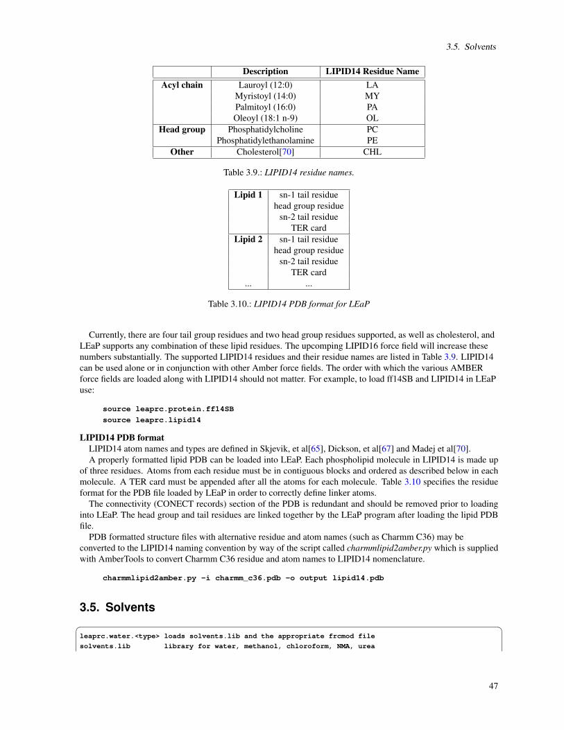
3.5. Solvents
Description LIPID14 Residue NameAcyl chain Lauroyl (12:0) LA
Myristoyl (14:0) MYPalmitoyl (16:0) PAOleoyl (18:1 n-9) OL
Head group Phosphatidylcholine PCPhosphatidylethanolamine PE
Other Cholesterol[70] CHL
Table 3.9.: LIPID14 residue names.
Lipid 1 sn-1 tail residuehead group residue
sn-2 tail residueTER card
Lipid 2 sn-1 tail residuehead group residue
sn-2 tail residueTER card
... ...
Table 3.10.: LIPID14 PDB format for LEaP
Currently, there are four tail group residues and two head group residues supported, as well as cholesterol, andLEaP supports any combination of these lipid residues. The upcomping LIPID16 force field will increase thesenumbers substantially. The supported LIPID14 residues and their residue names are listed in Table 3.9. LIPID14can be used alone or in conjunction with other Amber force fields. The order with which the various AMBERforce fields are loaded along with LIPID14 should not matter. For example, to load ff14SB and LIPID14 in LEaPuse:
source leaprc.protein.ff14SB
source leaprc.lipid14
LIPID14 PDB formatLIPID14 atom names and types are defined in Skjevik, et al[65], Dickson, et al[67] and Madej et al[70].A properly formatted lipid PDB can be loaded into LEaP. Each phospholipid molecule in LIPID14 is made up
of three residues. Atoms from each residue must be in contiguous blocks and ordered as described below in eachmolecule. A TER card must be appended after all the atoms for each molecule. Table 3.10 specifies the residueformat for the PDB file loaded by LEaP in order to correctly define linker atoms.
The connectivity (CONECT records) section of the PDB is redundant and should be removed prior to loadinginto LEaP. The head group and tail residues are linked together by the LEaP program after loading the lipid PDBfile.
PDB formatted structure files with alternative residue and atom names (such as Charmm C36) may beconverted to the LIPID14 naming convention by way of the script called charmmlipid2amber.py which is suppliedwith AmberTools to convert Charmm C36 residue and atom names to LIPID14 nomenclature.
charmmlipid2amber.py -i charmm_c36.pdb -o output lipid14.pdb
3.5. Solvents leaprc.water.<type> loads solvents.lib and the appropriate frcmod file
solvents.lib library for water, methanol, chloroform, NMA, urea
47

3. Molecular mechanics force fields
frcmod.tip4p Parameter changes for TIP4P.
frcmod.tip4pew Parameter changes for TIP4PEW.
frcmod.tip5p Parameter changes for TIP5P.
frcmod.spce Parameter changes for SPC/E.
frcmod.spceb Parameter changes for SPC/Eb.
frcmod.opc Parameter changes for OPC.
frcmod.pol3 Parameter changes for POL3.
frcmod.tip3pfb Parameter changes for the force-balance TIP3P model
frcmod.tip4pfb Parameter changes for the force-balance TIP4P model
frcmod.meoh Parameters for methanol.
frcmod.chcl3 Parameters for chloroform.
frcmod.nma Parameters for N-methyacetamide.
frcmod.urea Parameters for urea (or urea-water mixtures). Amber provides direct support for several water models. There is no default, but the most common water
model is TIP3P.[71] This model will be used for residues with names HOH or WAT. If you want to use otherwater models, execute the following leap commands after loading your leaprc file:
WAT = PL3 (residues named WAT in pdb file will be POL3)
source leaprc.water.pol3
(The above is obviously for the POL3 model.) The solvents.lib file contains TIP3P,[71] TIP3P/F,[72] TIP4P,[71,73] TIP4P/Ew,[74, 75] TIP5P,[76] OPC,[77] POL3[78], SPC/E[79], SPC/Eb[23], TIP3PFB[25] and TIP4PFB[25]models for water; these are called TP3, TPF, TP4, T4E, TP5, OPC, PL3, SPC, SPC, FB3 and FB4, respectively.(The SPC/E and SPC/Eb models are both called SPC: you just have to be sure to load the appropriate frcmod file.)By default, the residue name in the prmtop file will be WAT, regardless of which water model is used.
The “standard” leaprc files for tip3p, spce, tip4pew and opc also load the Joung/Cheatham monovalent ionparameters (see below). If you wish to use other parameters, or to deal with divalent or other ions, you will needto load the appropriate frcmod files.
Amber has two flexible water models, one for classical dynamics, SPC/Fw[80] (called “SPF”) and one forpath-integral MD, qSPC/Fw[81] (called “SPG”). You would use these in the following manner:
WAT = SPG
loadAmberParams frcmod.qspcfw
set default FlexibleWater on
Then, when you load a PDB file with residues called WAT, they will get the parameters for qSPC/Fw. (Obviously,you need to run some version of quantum dynamics if you are using qSPC/Fw water.)
The solvents.lib file, which is automatically loaded with many leaprc files, also contains pre-equilibrated boxesfor many of these water models. These are called POL3BOX, QSPCFWBOX, SPCBOX, SPCFWBOX, TIP3PBOX,TIP3PFBOX, TIP4PBOX, TIP4PEWBOX, OPCBOX, and TIP5PBOX. These can be used as arguments to the sol-vateBox or solvateOct commands in LEaP.
In addition, non-polarizable models for the organic solvents methanol, chloroform and N-methylacetamide areprovided,[82] along with a box for an 8M urea-water mixture. The input files for a single molecule are in $AMBER-HOME/dat/leap/prep, and the corresponding frcmod files are in $AMBERHOME/dat/leap/parm. Pre-equilibratedboxes are in $AMBERHOME/dat/leap/lib. For example, to solvate a simple peptide in methanol, you could do thefollowing: source leaprc.protein.ff14SB (get a standard force field)
loadAmberParams frcmod.meoh (get methanol parameters)
peptide = sequence ACE VAL NME (construct a simple peptide)
solvateBox peptide MEOHBOX 12.0 0.8 (solvate the peptide with meoh)
saveAmberParm peptide prmtop prmcrd
quit Similar commands will work for other solvent models.
48

3.6. Ions
3.5.1. OPC water model
OPC is a new non-polarizable, 4-point, 3-charge rigid water model.[77] Geometrically, it resembles TIP4P-likemodels, although the values of OPC point charges and charge-charge distances are quite different. The model hasa single VDW center on the oxygen nucleus. The model is constructed based on the concept of optimal pointcharge approximation; [83] the central idea of OPC is to distribute the point charges to best reproduce the 3 lowestorder multipole moments of water molecule in liquid phase. The optimal values for the dipole µ and the squarequadrupole moment QT [84] are determined as best fit values that reproduce key experimental properties of water inliquid phase. The low dimensionality of the parameter space µ-QT permits a virtually exhaustive search. The linearquadrupole and the octupole moments[85] are fixed to values obtained from high quality QM calculations.[84]
A full description of OPC and its properties can be found in Ref.[77]. For 11 key liquid state properties againstwhich water models are most often benchmarked, OPC is on average within 0.76% of the experiment (relativeerror). This accuracy is dramatically better compared to the commonly used rigid models. For example, thedielectric constant of TIP3P and TIP4PEw is 94 and 63.9 respectively, while OPC predicts it to be 78.4±0.6 (theexperimental value is 78.4). The reported OPC properties were computed using Amber 12 on GPUs with a time-step of 2 fs, periodic boundary conditions, an 8 angstrom cut-off for nonbonded interactions, and PME for longrange electrostatics. SHAKE was used to constrain hydrogens. The rest of parameters are set to current Amberdefaults; note that these include accounting for the van der Waals interactions beyond the cut-off via a continuummodel (vdwmeth=1).
Because of the improved accuracy in bulk properties, OPC delivers noticeable accuracy improvement in practicalatomistic simulations, even with existing force-fields. Improvements were reported in: RNA simulations,[86]thermodynamics of ligand binding,[87] small molecule hydration,[77] and simulations of intrinsically disorderedproteins (unpublished).
Two sets of 12-6 LJ parameters for OPC water model (the 12-6 IOD set and the 12-6 HFE set) for 3 monovalentions (Na+, K+, Cl-) have been developed by Li, Merz and co-workers, see Section 3.6 for the definition andimportant usage suggestions. Our tests show that the deviation of the Ion-Oxygen Distances predicted using the 12-6 HFE set from the reference IOD values is within ±0.2A. Comparing these deviations to those reported for otherion parameter sets available, it seems that the magnitude of the deviation is borderline acceptable, which meansthat the HFE set might also work in situations where IOD is formally recommended. For Na+ the transferability isnot an issue as HFE and IOD parameters are essentially the same. In situations where agreement of HFEs with oneof the common experimental references is critical, the use of OPC-specific parameters (the 12-6 HFE set) for K+,Na+, and Cl- may be advisable. The IOD parameter set are recommended to be used in the structural refinement.
Based on our limited experience, it appears that the Joung/Cheatham ion parameters for TIP4P-EW (jc_tip4pew)[88]may also be acceptable for OPC water model, especially when accurate reproduction of IODs is critical. One ad-vantage of using the jc_tip4pew set is that it provides a consistent set of parameters for most biologically relevantions, not just K+, Na+, and Cl-. Another advantage at the moment is that the set has already been tested in practicewith OPC model.[86, 87]
3.6. Ions frcmod.ionsjc_tip3p Joung/Cheatham ion parameters for TIP3P water
frcmod.ionsjc_spce same, but for SPC/E water
frcmod.ionsjc_tip4pew same, but for TIP4P/EW water
frcmod.ions1lm_126_tip3p Li/Merz ion parameters for +1 and -1 ions in TIP3P water (12-6 normal usage set)
frcmod.ions1lm_126_spce same, but in SPC/E water
frcmod.ions1lm_126_tip4pew same, but in TIP4P/EW water
frcmod.ions1lm_iod Li/Merz ion parameters for +1 and -1 ions (12-6 IOD set)
frcmod.ions234lm_126_tip3p Li/Merz ion parameters for +2 to +4 ions in TIP3P water (12-6 normal usage set)
frcmod.ions234lm_126_spce same, but in SPC/E water
frcmod.ions234lm_126_tip4pew same, but in TIP4P/EW water
frcmod.ions234lm_hfe_tip3p Li/Merz ion parameters for +2 to +4 ions in TIP3P water (12-6 HFE set)
49

3. Molecular mechanics force fields
frcmod.ions234lm_hfe_spce same, but in SPC/E water
frcmod.ions234lm_hfe_tip4pew same, but in TIP4PEW water
frcmod.ions234lm_iod_tip3p Li/Merz ion parameters for +2 to +4 ions in TIP3P water (12-6 IOD set)
frcmod.ions234lm_iod_spce same, but in SPC/E water
frcmod.ions234lm_iod_tip4pew same, but in TIP4P/EW water
frcmod.ions1lm_1264_tip3p Li/Merz ion parameters for -1 and +1 ions in TIP3P water (12-6-4 set)
frcmod.ions1lm_1264_spce same, but in SPC/E water
frcmod.ions1lm_1264_tip4pew same, but in TIP4PEW water
frcmod.ions234lm_1264_tip3p Li/Merz ion parameters for +2 to +4 ions in TIP3P water (12-6-4 set)
frcmod.ions234lm_1264_spce same, but in SPC/E water
frcmod.ions234lm_1264_tip4pew same, but in TIP4PEW water
frcmod.ions1lm_126_hfe_opc Li/Merz ion parameters for +1 and -1 ions in OPC water (12-6 HFE set)
frcmod.ions1lm_126_iod_opc Li/Merz ion parameters for +1 and -1 ions in OPC water (12-6 IOD set)
atomic_ions.lib topologies for monoatomic ions (new naming scheme)
ions94.lib topologies for ions with the old naming scheme In 2008, Joung and Cheatham created a consistent set of parameters for alkali halide ions, fitting solvation
free energies, radial distribution functions, ion-water interaction energies and crystal lattice energies and latticeconstants for non-polarizable spherical ions.[88, 89] These have been separately parametrized for each of threepopular water models, as indicated above.
Li, Merz and co-workers subsequently developed ion parameters for the monovalent, divalent, trivalent andtetravalent ions for the 12-6 LJ nonbonded model and the 12-6-4 LJ-type nonbonded model for PME simulations.[90–93] The experimental values they tried to reproduce are the experimental Hydration Free Energy (HFE) values,Ion-Oxygen Distance (IOD) values and Coordination Number (CN) values of the first solvation shell. It was foundthat it is hard to reproduce the three experimental values simultaneously by using the 12-6 LJ nonbonded model.Since the charge-induced dipole interaction is proportional tor−4 , a new term with format (C/r)4 was added tothe 12-6 LJ potential, yielding a 12-6-4 LJ-type potential. The new potential with designed parameters could re-produce the experimental HFE, IOD and CN values at the same time without significant compromise. Especiallyfor the highly charged metal ions, the 12-6-4 LJ-type nonbonded model performs much better than the 12-6 oneoverall. Similar to Joung and Cheatam’s work, three water models were treated separately for the parameter design,as indicated in the name of frcmod files. Users can check the notes in the frcmod files to see the reference of eachparameter.
For the 12-6 LJ nonbonded model, three different parameter sets are avaliable for each water model to meetdifferent requirements:
1. 12-6 normal usage set. In which we have HFE set of the monovalent ions (could reproduce the experimentalHFE),[93] the Compromise (CM) set of divalent ions (which could reproduce the experimental relative HFEand CN values),[91] and IOD set (could reproduce the experimental IOD) for the trivalent and tetravalentions.[92] These parameters are recommended to be used in the normal MD simulations. This is becausefor the monovalent ions the error of the 12-6 LJ nonbonded model is pretty small (a CM set may not neededsince HFE or IOD set are pretty close to each other) while for the trivalent and tetravalent metal ions the12-6 LJ nonboned model has relative big error (a CM set could have big error for both HFE and IOD at thismoment).
2. 12-6 HFE set to reproduce experimental HFE.[90, 92, 93] The HFE parameter set has limited error formonovalent ions, while could have remarkable error for highly charged ions. Since we use the HFE setfor monovalent ions in the 12-6 normal usage set, so we don’t have a sepecific HFE set parameter file formonovalent ions.
3. 12-6 IOD set to reproduce experimental IOD.[90, 92, 93] Since the ion with certain parameter could repro-duce similar IOD values in the three water models, so the IOD set parameters of three water models weredesigned identical (for the monovalent and divalent metal ions, while for the trivalent and tetravalent ions,
50

3.7. Modified amino acids and nucleotides
the IOD set are estimated for each water model separately). The IOD parameter set are recommended tobe used in the structural refinement or for structural property orientated investigation.
For the 12-6-4 LJ-type nobonded model, only one parameter set (12-6-4 set) designed for each of the three wa-ter models. The 12-6-4 model has also been tested in mixed systems (such as nucleic acids, proteins and ionicsolutions) and have shown excellent transferability.[91–93] In the recent work of Panteva et al. found the 12-6-4model gives improved results over the 12-6 model when modeling Mg2+ with nucleic acid systems. Additionally,the 12-6-4 model with the SPC/E water model performed exceptionally well for simulating all properties in thesebenchmark calculations.[94] The VDW parameters which specified designed for the divalent metal ions with 12-6-4 LJ-type nonbonded model are shown as the 12-6-4 set in the above. These frcmod files can be used to generatean original prmtop file. After obtaining the original prmtop file, you can use the add12_6_4 command in parmedto generate a prmtop with the additionalC4 terms with the flag LENNARD_JONES_CCOEF. Please see the add12_6_4command14.2.2.6 in Subsection14.2.2 in the manual for detailed information. After obtaining the prmtop with theadditional C4 term, you can use sander or pmemd to run the simulation. Recently Penteva et al. fine-tuned theC4terms between several divalent metal ions (Mg2+, Mn2+, Zn2+, and Cd2+ ) and nucleic acid systems[95] while keeptheC4 terms between metal ions and water desgined by Li and Merz.[91] The new parameter set could better bal-ance the interaction types in the nucleic acid systems and are recommended to use in related modeling. An relatedtutorial is shown in the following webpage: "http://ambermd.org/tutorials/advanced/tutorial20/12_6_4.htm".
3.7. Modified amino acids and nucleotides
Parameters for phosphorylated amino acids [96, 97] can be obtained by typing “source leaprc.phophaa10” inyour leap.in file. Many post-translational modifications are also available at http://selene.princeton.edu/FFPTM/.Parameters for common modifications for RNA nucleotides [45]can by loaded with “source leaprc.modrna08”.Pointers to other sets of Amber-compatible force fields may be found at the Amber web site, http://ambermd.org/.
Additional parameters for six common fluorescent protein chromophores–eGFP, eBFP, eYFP, eCFP, DsRed, andmCherry–are available[98] by sourcing leaprc.xFPchromophores after sourcing the main force field leaprc file (e.g.leaprc.protein.ff14SB). This will allow seamless loading of PDB files containing fluorescent proteins provided theyfollow standard naming of the chromophore: eGFP=CRO, eBFP=IIC, eYFP=CR2, eCFP=CRF, DsRed= CRQ, andmCherry=CH6. The chromophore parmaeters are based on parm10 with the ff14SB modifications, but also borrowheavily from GAFF. Both uppercase and lowercase atom types are utilized, so users should take caution if mixingff14SB with GAFF. See original reference[98] for details of implementation.
3.8. Force fields related to semi-empirical QM
ParmAM1 and parmPM3 are classical force field parameter sets that reproduce the geometry of proteinsminimized at the semi-empirical AM1 or PM3 level, respectively.[99] These new force fields provide aninexpensive, yet reliable, method to arrive at geometries that are more consistent with a semi-empirical treatmentof protein structure. These force fields are meant only to reproduce AM1 and PM3 geometries (warts and all) andwere not tested for use in other instances (e.g., in classical MD simulations, etc.) Since the minimization of aprotein structure at the semi-empirical level can become cost-prohibitive, a “preminimization” with anappropriately parametrized classical treatment will facilitate future analysis using AM1 or PM3 Hamiltonians.
3.9. Obsolete force field files
The following files are included for historical interest. We do not recommend that these be used any more formolecular simulations. The leaprc files that load these files have been moved to $AMBERHOME/dat/leap/par-m/oldff.
51

3. Molecular mechanics force fields
3.9.1. The Weiner et al. (1984,1986) force fields all.in All atom database input.
allct.in All atom database input, COO- Amino acids.
allnt.in All atom database input, NH3+ Amino acids.
uni.in United atom database input.
unict.in United atom database input, COO- Amino acids.
unint.in United atom database input, NH3+ Amino acids.
parm91X.dat Parameters for 1984, 1986 force fields. The ff86 parameters are described in early papers from the Kollman and Case groups.[100, 101] [The “parm91”
designation is somewhat unfortunate: this file is really only a corrected version of the parameters described inthe 1984 and 1986 papers listed above.] These parameters are not generally recommended any more, but maystill be useful for vacuum simulations of nucleic acids and proteins using a distance-dependent dielectric, or forcomparisons to earlier work. The material in parm91X.dat is the parameter set distributed with Amber 4.0. TheSTUB nonbonded set has been copied from parmuni.dat; these sets of parameters are appropriate for united atomcalculations using the “larger” carbon radii referred to in the “note added in proof” of the 1984 JACS paper. Ifthese values are used for a united atom calculation, the parameter scnb must be defined in the prmtop file andshould be set to 8.0; for all-atom calculations it should be 2.0. The scee parameter should be defined in the prmtopfile and set to 2.0 for both united atom and all-atom variants. Note that the default value for scee is now 1.2 (thevalue for 1994 and later force fields); this must be explicitly defined in the prmtop file when using the earlier forcefields.
parm91X.dat is not recommended. However, for historical completeness a number of terms in the non-bondedlist of parm91X.dat should be noted. The non-bonded terms for I (iodine), CU (copper) and MG (magnesium) havenot been carefully calibrated, but are given as approximate values. In the STUB set of non-bonded parameters, wehave included parameters for a large hydrated monovalent cation (IP) that represent work by Singh et al.[102] onlarge hydrated counterions for DNA. Similar values are included for a hydrated anion (IM).
The non-bonded potentials for hydrogen-bond pairs in ff86 use a Lennard-Jones 10-12 potential. If you want torun sander with ff86 then you will need to recompile, adding -DHAS_10_12 to the Fortran preprocessor flags.
3.9.2. The Cornell et al. (1994) force field all_nuc94.in Nucleic acid input for building database.
all_amino94.in Amino acid input for building database.
all_aminoct94.in COO- amino acid input for database.
all_aminont94.in NH3+ amino acid input for database.
nacl.in Ion file.
parm94.dat 1994 force field file.
parm96.dat Modified version of 1994 force field, for proteins.
parm98.dat Modified version of 1994 force field, for nucleic acids. Contained in ff94 are parameters from the so-called “second generation” force field developed in the Kollman
group in the early 1990s.[24] These parameters are especially derived for solvated systems, and when used with anappropriate 1-4 electrostatic scale factor, have been shown to perform well at modeling many organic molecules.The parameters in parm94.dat omit the hydrogen bonding terms of earlier force fields. This is an all-atom forcefield; no united-atom counterpart is provided. 1-4 electrostatic interactions are scaled by 1.2 instead of the valueof 2.0 that had been used in earlier force fields.
Charges were derived using Hartree-Fock theory with the 6-31G* basis set, because this exaggerates the dipolemoment of most residues by 10-20%. It thus “builds in” the amount of polarization which would be expected inaqueous solution. This is necessary for carrying out condensed phase simulations with an effective two-body forcefield which does not include explicit polarization. The charge-fitting procedure is described in Ref [24].
The ff96 force field [103] differs from parm94.dat in that the torsions for φ and ψ have been modified inresponse to ab initio calculations [104] which showed that the energy difference between conformations werequite different than calculated by Cornell et al. (using parm94.dat). To create parm96.dat, common V1 and V2
52

3.9. Obsolete force field files
parameters were used for φ and ψ , which were empirically adjusted to reproduce the energy difference betweenextended and constrained alpha helical energies for the alanine tetrapeptide. This led to a significant improvementbetween molecular mechanical and quantum mechanical relative energies for the remaining members of the set oftetrapeptides studied by Beachy et al. Users should be aware that parm96.dat has not been as extensively usedas parm94.dat, and that it almost certainly has its own biases and idiosyncrasies, including strong bias favoringextended β conformations.[17, 105, 106]
The ff98 force field [107] differs from parm94.dat in torsion angle parameters involving the glycosidic torsionin nucleic acids. These serve to improve the predicted helical repeat and sugar pucker profiles.
3.9.3. The Wang et al. (1999) force field parm99.dat Basic force field parameters
all_amino94.in topologies and charges for amino acids
all_amino94nt.in same, for N-terminal amino acids
all_amino94ct.in same, for C-terminal amino acids
all_nuc94.in topologies and charges for nucleic acids
gaff.dat Force field for general organic molecules
all_modrna08.lib topologies for modified nucleosides
all_modrna08.frcmod parameters for modified nucleosides The ff99 force field [108] points toward a common force field for proteins for “general” organic and bio-organic
systems. The atom types are mostly those of Cornell et al. (see below), but changes have been made in manytorsional parameters. The topology and coordinate files for the small molecule test cases used in the developmentof this force field are in the parm99_lib subdirectory. The ff99 force field uses these parameters, along with thetopologies and charges from the Cornell et al. force field, to create an all-atom nonpolarizable force field forproteins and nucleic acids.
There are more than 99 naturally occurring modifications in RNA. Amber force field parameters for all thesemodifications have been developed to be consistent with ff94 and ff99.[45] The modular nature of RNA was takeninto consideration in computing the atom-centered partial charges for these modified nucleosides, based on thecharging model for the “normal” nucleotides.[109] All the ab initio calculations were done at the Hartree-Focklevel of theory with 6-31G(d) basis sets, using the GAUSSIAN suite of programs. The computed electrostaticpotential (ESP) was fit using RESP charge fitting in antechamber. Three-letter codes for all of the fitted nucleosideswere developed to standardize the naming of the modified nucleosides in PDB files. For a detailed description ofcharge fitting for these nucleosides and an outline for the three letter codes, please refer to Ref. [45].
The AMBER force field parameters for 99 modified nucleosides are distributed in the form of library files. Theall_modrna08.lib file contains coordinates, connectivity, and charges, and all_modrna08.frcmod contains infor-mation about bond lengths, angles, dihedrals and others. The AMBER force field parameters for the 99 modifiednucleosides in RNA are also maintained at the modified RNA database at http://ozone3.chem.wayne.edu.
3.9.4. The 2002 polarizable force fields frcmod.ff02pol.r1 Recommended initialization file
parm99.dat Force field, for amino acids and some organic molecules;
can be used with either additive or
non-additive treatment of electrostatics.
parm99EP.dat Like parm99.dat, but with "extra-points": off-center
atomic charges, somewhat like lone-pairs.
frcmod.ff02pol.r1 Updated torsion parameters for ff02.
all_nuc02.in Nucleic acid input for building database, for a non-
additive (polarizable) force field without extra points.
all_amino02.in Amino acid input ...
all_aminoct02.in COO- amino acid input ...
all_aminont02.in NH3+ amino acid input ....
all_nuc02EP.in Nucleic acid input for building database, for a non-
53
3. Molecular mechanics force fields
additive (polarizable) force field with extra points.
all_amino02EP.in Amino acid input ...
all_aminoct02EP.in COO- amino acid input ...
all_aminont02EP.in NH3+ amino acid input .... The ff02 force field is a polarizable variant of ff99. (See Ref. [110] for a recent overview of polarizable force
fields.) Here, the charges were determined at the B3LYP/cc-pVTZ//HF/6-31G* level, and hence are more like “gas-phase” charges. During charge fitting the correction for intramolecular self polarization has been included.[82]Bond polarization arising from interactions with a condensed phase environment are achieved through polarizabledipoles attached to the atoms. These are determined from isotropic atomic polarizabilities assigned to each atom,taken from experimental work of Applequist. The dipoles can either be determined at each step through an iterativescheme, or can be treated as additional dynamical variables, and propagated through dynamics along with theatomic positions, in a manner analogous to Car-Parinello dynamics. Derivation of the polarizable force fieldrequired only minor changes in dihedral terms and a few modification of the van der Waals parameters.
Subsequently, a set up updated torsion parameters has been developed for the ff02 polarizable force field.[111]These are available in the frcmod.ff02pol.r1 file.
The user also has a choice to use the polarizable force field with extra points on which additional point chargesare located; this is called ff02EP. The additional points are located on electron donating atoms (e.g. O,N,S), whichmimic the presence of electron lone pairs.[112] For nucleic acids we chose to use extra interacting points only onnucleic acid bases and not on sugars or phosphate groups.
There is not (yet) a full published description of this, but a good deal of preliminary work on small moleculesis available.[82, 113] Beyond small molecules, our initial tests have focused on small proteins and double helicaloligonucleotides, in additive TIP3P water solution. Such a simulation model, (using a polarizable solute in a non-polarizable solvent) gains some of the advantages of polarization at only a small extra cost, compared to a standardforce field model. In particular, the polarizable force field appears better suited to reproduce intermolecular inter-actions and directionality of H-bonding in biological systems than the additive force field. Initial tests show ff02EPbehaves slightly better than ff02, but it is not yet clear how significant or widespread these differences will be.
3.9.5. Older ion parameters
In the past, for alkali ions with TIP3P waters, Amber has provided the values of Aqvist,[114] adjusted forAmber’s nonbonded atom pair combining rules to give the same ion-OW potentials as in the original (which weredesigned for SPC water); these values reproduce the first peak of the radial distribution for ion-OW and the relativefree energies of solvation in water of the various ions. Note that these values would have to be changed if awater model other than TIP3P were to be used. Rather arbitrarily, Amber also included chloride parameters fromDang.[115] These are now known not to work all that well with the Aqvist cation parameters, particularly for theK/Cl pair. Specifically, at concentrations above 200 mM, KCl will spontaneously crystallize; this is also seen withNaCl at concentrations above 1 M.[116] These “older” parameters are now collected in frcmod.ionsff99_tip3p, butare not recommended except to reproduce older simulations.
54
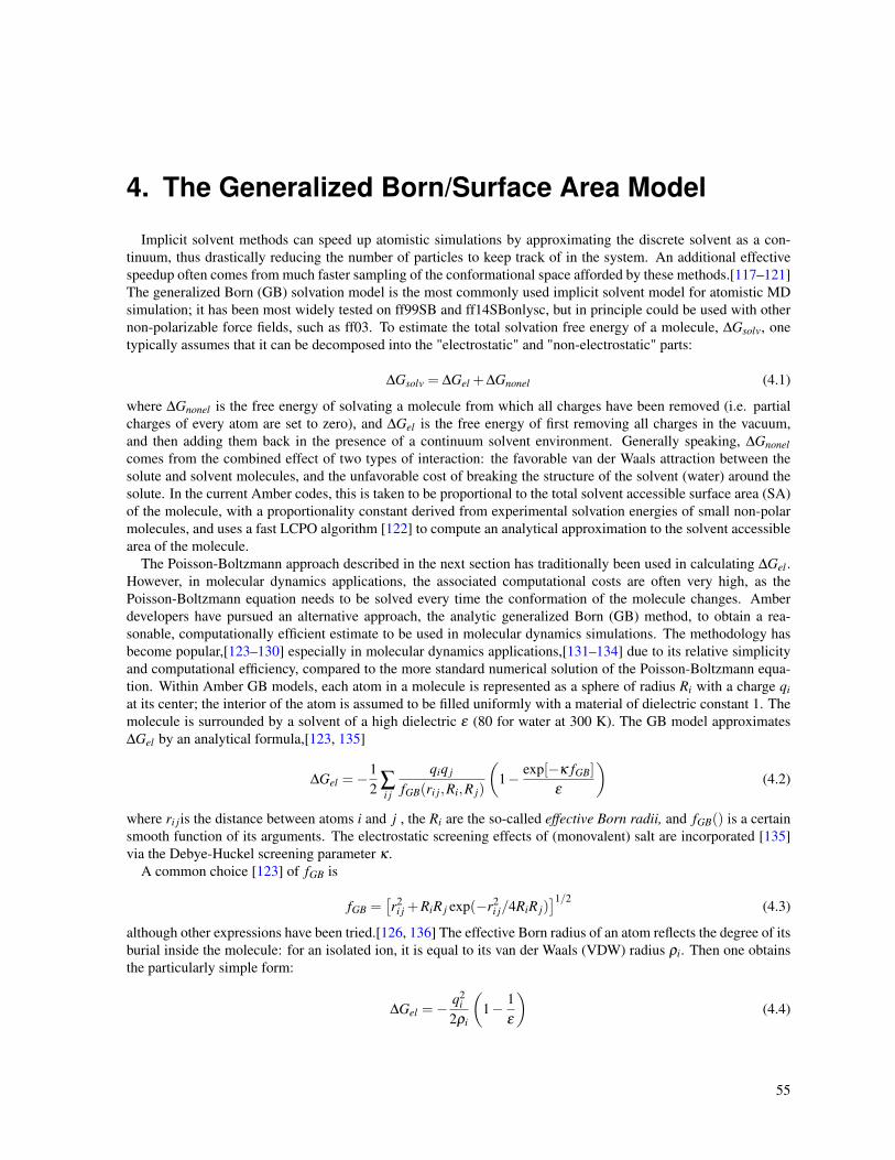
4. The Generalized Born/Surface Area Model
Implicit solvent methods can speed up atomistic simulations by approximating the discrete solvent as a con-tinuum, thus drastically reducing the number of particles to keep track of in the system. An additional effectivespeedup often comes from much faster sampling of the conformational space afforded by these methods.[117–121]The generalized Born (GB) solvation model is the most commonly used implicit solvent model for atomistic MDsimulation; it has been most widely tested on ff99SB and ff14SBonlysc, but in principle could be used with othernon-polarizable force fields, such as ff03. To estimate the total solvation free energy of a molecule, ∆Gsolv, onetypically assumes that it can be decomposed into the "electrostatic" and "non-electrostatic" parts:
∆Gsolv = ∆Gel +∆Gnonel (4.1)
where ∆Gnonel is the free energy of solvating a molecule from which all charges have been removed (i.e. partialcharges of every atom are set to zero), and ∆Gel is the free energy of first removing all charges in the vacuum,and then adding them back in the presence of a continuum solvent environment. Generally speaking, ∆Gnonelcomes from the combined effect of two types of interaction: the favorable van der Waals attraction between thesolute and solvent molecules, and the unfavorable cost of breaking the structure of the solvent (water) around thesolute. In the current Amber codes, this is taken to be proportional to the total solvent accessible surface area (SA)of the molecule, with a proportionality constant derived from experimental solvation energies of small non-polarmolecules, and uses a fast LCPO algorithm [122] to compute an analytical approximation to the solvent accessiblearea of the molecule.
The Poisson-Boltzmann approach described in the next section has traditionally been used in calculating ∆Gel .However, in molecular dynamics applications, the associated computational costs are often very high, as thePoisson-Boltzmann equation needs to be solved every time the conformation of the molecule changes. Amberdevelopers have pursued an alternative approach, the analytic generalized Born (GB) method, to obtain a rea-sonable, computationally efficient estimate to be used in molecular dynamics simulations. The methodology hasbecome popular,[123–130] especially in molecular dynamics applications,[131–134] due to its relative simplicityand computational efficiency, compared to the more standard numerical solution of the Poisson-Boltzmann equa-tion. Within Amber GB models, each atom in a molecule is represented as a sphere of radius Ri with a charge qiat its center; the interior of the atom is assumed to be filled uniformly with a material of dielectric constant 1. Themolecule is surrounded by a solvent of a high dielectric ε (80 for water at 300 K). The GB model approximates∆Gel by an analytical formula,[123, 135]
∆Gel =−12 ∑
i j
qiq j
fGB(ri j,Ri,R j)
(1− exp[−κ fGB]
ε
)(4.2)
where ri jis the distance between atoms i and j , the Ri are the so-called effective Born radii, and fGB() is a certainsmooth function of its arguments. The electrostatic screening effects of (monovalent) salt are incorporated [135]via the Debye-Huckel screening parameter κ .
A common choice [123] of fGB is
fGB =[r2
i j +RiR j exp(−r2i j/4RiR j)
]1/2(4.3)
although other expressions have been tried.[126, 136] The effective Born radius of an atom reflects the degree of itsburial inside the molecule: for an isolated ion, it is equal to its van der Waals (VDW) radius ρi. Then one obtainsthe particularly simple form:
∆Gel =−q2
i2ρi
(1− 1
ε
)(4.4)
55

4. The Generalized Born/Surface Area Model
where we assumed κ = 0 (pure water). This is the famous expression due to Born for the solvation energy ofa single ion. The function fGB() is designed to interpolate, in a clever manner, between the limit ri j → 0, whenatomic spheres merge into one, and the opposite extreme ri j → ∞, when the ions can be treated as point chargesobeying the Coulomb’s law.[129] For deeply buried atoms, the effective radii are large, Ri ρi, and for such atomsone can use a rough estimate Ri ≈ Li, where Li is the distance from the atom to the molecular surface. Closer tothe surface, the effective radii become smaller, and for a completely solvent exposed side-chain one can expect Rito approach ρi.
The effective radii depend on the molecule’s conformation, and so have to be re-computed every time the confor-mation changes. This makes the computational efficiency a critical issue, and various approximations are normallymade that facilitate an effective estimate of Ri. With an exception of GBNSR6 (see Section 5.1), the so-calledCoulomb field approximation, or CFA, is used for Amber GB models, which replaces the true electric displace-ment around the atom by the Coulomb field. Within this assumption, the following expression can be derived:[129]
R−1i = ρ
−1i −
14π
∫θ(|r|−ρi)r−4dr (4.5)
where the integral is over the solute volume surrounding atom i. For a realistic molecule, the solute boundary(molecular surface) is anything but trivial, and so further approximations are made to obtain a closed-form ana-lytical expression for the above equation, e.g. the so-called pairwise de-screening approach of Hawkins, Cramerand Truhlar,[137] which leads to a GB model implemented in Amber with igb=1. The 3D integral used in theestimation of the effective radii is performed over the van der Waals (VDW) spheres of solute atoms, which im-plies a definition of the solute volume in terms of a set of spheres, rather than the complex molecular surface,[138]commonly used in the PB calculations. For macromolecules, this approach tends to underestimate the effectiveradii for buried atoms,[129] arguably because the standard integration procedure treats the small vacuum–filledcrevices between the van der Waals (VDW) spheres of protein atoms as being filled with water, even for struc-tures with large interior.[136] This error is expected to be greatest for deeply buried atoms characterized by largeeffective radii, while for the surface atoms it is largely canceled by the opposing error arising from the Coulombapproximation, which tends [124, 128, 139] to overestimate Ri.
The deficiency of the model described above can, to some extent, be corrected by noticing that even the opti-mal packing of hard spheres, which is a reasonable assumption for biomolecules, still occupies only about threequarters of the space, and so "scaling-up" of the integral by a factor of four thirds should effectively increase theunderestimated radii by about the right amount, without any loss of computational efficiency. This idea was devel-oped and applied in the context of pH titration,[129] where it was shown to improve the performance of the GBapproximation in calculating pKa values of protein sidechains. However, the one-parameter correction introducedin Ref. [129] was not optimal in keeping the model’s established performance on small molecules. It was thereforeproposed [134] to re-scale the effective radii with the re-scaling parameters being proportional to the degree of theatom’s burial, as quantified by the value Ii of the 3D integral. The latter is large for the deeply buried atoms andsmall for exposed ones. Consequently, one seeks a well-behaved re-scaling function, such that Ri ≈ (ρ−1
i − Ii)−1
for small Ii, and Ri > (ρ−1i − Ii)
−1 when Ii becomes large. The following simple, infinitely differentiable re-scalingfunction was chosen to replace the model’s original expression for the effective radii:
R−1i = ρ
−1i −ρ
−1i tanh(αΨ−βΨ
2 + γΨ3) (4.6)
where Ψ = Iiρi, and α , β , γ are treated as adjustable dimensionless parameters which were optimized using theguidelines mentioned earlier (primarily agreement with the PB). Currently, Amber supports two GB models (termed OBC ) based on this idea. These differ by the values of α , β , γ , and are invoked by setting igb to eitherigb=2 or igb=5. The details of the optimization procedure and the performance of the OBC model relative to thePB treatment and in MD simulations on proteins is described in Ref. [134]; an independent comparison to the PBin calculating the electrostatic part of solvation free energy on a large data set of proteins can be found in Ref.[140].
Our experience with generalized Born simulations is mainly with ff99SB, ff14SBonlysc or ff03; the current GBmodels are not compatible with polarizable force fields. Replacing explicit water with a GB model is equivalent tospecifying a different force field, and users should be aware that none of the GB options (in Amber or elsewhere)is as mature as simulations with explicit solvent; user discretion is advised. For example, it was shown that
56
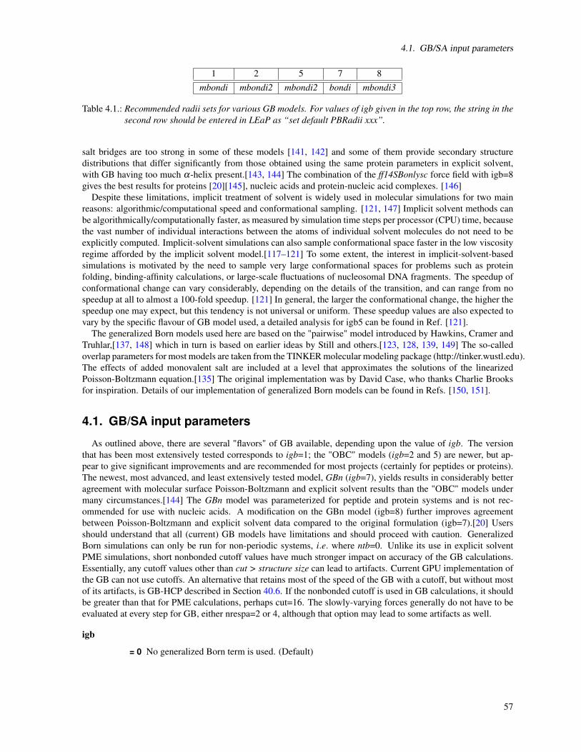
4.1. GB/SA input parameters
1 2 5 7 8mbondi mbondi2 mbondi2 bondi mbondi3
Table 4.1.: Recommended radii sets for various GB models. For values of igb given in the top row, the string in thesecond row should be entered in LEaP as “set default PBRadii xxx”.
salt bridges are too strong in some of these models [141, 142] and some of them provide secondary structuredistributions that differ significantly from those obtained using the same protein parameters in explicit solvent,with GB having too much α-helix present.[143, 144] The combination of the ff14SBonlysc force field with igb=8gives the best results for proteins [20][145], nucleic acids and protein-nucleic acid complexes. [146]
Despite these limitations, implicit treatment of solvent is widely used in molecular simulations for two mainreasons: algorithmic/computational speed and conformational sampling. [121, 147] Implicit solvent methods canbe algorithmically/computationally faster, as measured by simulation time steps per processor (CPU) time, becausethe vast number of individual interactions between the atoms of individual solvent molecules do not need to beexplicitly computed. Implicit-solvent simulations can also sample conformational space faster in the low viscosityregime afforded by the implicit solvent model.[117–121] To some extent, the interest in implicit-solvent-basedsimulations is motivated by the need to sample very large conformational spaces for problems such as proteinfolding, binding-affinity calculations, or large-scale fluctuations of nucleosomal DNA fragments. The speedup ofconformational change can vary considerably, depending on the details of the transition, and can range from nospeedup at all to almost a 100-fold speedup. [121] In general, the larger the conformational change, the higher thespeedup one may expect, but this tendency is not universal or uniform. These speedup values are also expected tovary by the specific flavour of GB model used, a detailed analysis for igb5 can be found in Ref. [121].
The generalized Born models used here are based on the "pairwise" model introduced by Hawkins, Cramer andTruhlar,[137, 148] which in turn is based on earlier ideas by Still and others.[123, 128, 139, 149] The so-calledoverlap parameters for most models are taken from the TINKER molecular modeling package (http://tinker.wustl.edu).The effects of added monovalent salt are included at a level that approximates the solutions of the linearizedPoisson-Boltzmann equation.[135] The original implementation was by David Case, who thanks Charlie Brooksfor inspiration. Details of our implementation of generalized Born models can be found in Refs. [150, 151].
4.1. GB/SA input parameters
As outlined above, there are several "flavors" of GB available, depending upon the value of igb. The versionthat has been most extensively tested corresponds to igb=1; the "OBC" models (igb=2 and 5) are newer, but ap-pear to give significant improvements and are recommended for most projects (certainly for peptides or proteins).The newest, most advanced, and least extensively tested model, GBn (igb=7), yields results in considerably betteragreement with molecular surface Poisson-Boltzmann and explicit solvent results than the "OBC" models undermany circumstances.[144] The GBn model was parameterized for peptide and protein systems and is not rec-ommended for use with nucleic acids. A modification on the GBn model (igb=8) further improves agreementbetween Poisson-Boltzmann and explicit solvent data compared to the original formulation (igb=7).[20] Usersshould understand that all (current) GB models have limitations and should proceed with caution. GeneralizedBorn simulations can only be run for non-periodic systems, i.e. where ntb=0. Unlike its use in explicit solventPME simulations, short nonbonded cutoff values have much stronger impact on accuracy of the GB calculations.Essentially, any cutoff values other than cut > structure size can lead to artifacts. Current GPU implementation ofthe GB can not use cutoffs. An alternative that retains most of the speed of the GB with a cutoff, but without mostof its artifacts, is GB-HCP described in Section 40.6. If the nonbonded cutoff is used in GB calculations, it shouldbe greater than that for PME calculations, perhaps cut=16. The slowly-varying forces generally do not have to beevaluated at every step for GB, either nrespa=2 or 4, although that option may lead to some artifacts as well.
igb
= 0 No generalized Born term is used. (Default)
57

4. The Generalized Born/Surface Area Model
= 1 The Hawkins, Cramer, Truhlar[137, 148] pairwise generalized Born model is used, with param-eters described by Tsui and Case.[150] This model uses the default radii set up by LEaP. It isslightly different from the GB model that was included in Amber6. If you want to compare toAmber 6, or need to continue an ongoing simulation, you should use the command "set defaultPBradii amber6" in LEaP, and set igb=1 in sander. For reference, the Amber6 values are thoseused by an earlier Tsui and Case paper.[132] Note that most nucleic acid simulations have usedthis model, so you take care when using other values. Also note that Tsui and Case used an offset(see below) of 0.13 Å, which is different from its default value.
= 2 Use a modified GB model developed by A. Onufriev, D. Bashford and D.A. Case; the main ideawas published earlier,[129] but the actual implementation here[134] is an elaboration of thisinitial idea. Within this model, the effective Born radii are re-scaled to account for the interstitialspaces between atom spheres missed by the GBHCT approximation. In that sense, GBOBC isintended to be a closer approximation to true molecular volume, albeit in an average sense. Withigb=2, the inverse of the effective Born radius is given
by:cedure
R−1i = ρ
−1i − tanh
(αΨ−βΨ2 + γΨ3
)/ρi
where ρ i = ρi − o f f set, and Ψ = Iρi, with I given in our earlier paper. The parameters α ,β , and γ were determined by empirical fits, and have the values 0.8, 0.0, and 2.909125. Thiscorresponds to model I in Ref [134]. With this option, you should use the LEaP command "setdefault PBradii mbondi2" to prepare the prmtop file.
= 3 or 4 These values are unused; they were used in Amber 7 for parameter sets that are no longersupported.
= 5 Same as igb=2, except that now α,β ,γ are 1.0, 0.8, and 4.85. This corresponds to model II inRef [134]. With this option, you should use the command "set default PBradii mbondi2" insetting up the prmtop file, although "set default PBradii bondi" is also OK. When tested in MDsimulations of several proteins,[134] both of the above parameterizations of the "OBC" modelshowed equal performance, although further tests [140] on an extensive set of protein structuresrevealed that the igb=5 variant agrees better with the Poisson-Boltzmann treatment in calculatingthe electrostatic part of the solvation free energy.
= 6 With this option, there is no continuum solvent model used at all; this corresponds to a non-periodic, "vacuum", model where the non-bonded interactions are just Lennard-Jones and Coulombinteractions. This option is logically equivalent to setting igb=0 and eedmeth=4, although theimplementation (and computational efficiency) is not the same.
= 7 The GBn model described by Mongan, Simmerling, McCammon, Case and Onufriev[152] isemployed. This model uses a pairwise correction term to GBHCT to approximate a molecularsurface dielectric boundary; that is to eliminate interstitial regions of high dielectric smaller thana solvent molecule. This correction affects all atoms and is geometry-specific, going beyondthe geometry-free, "average" re-scaling approach of GBOBC, which mostly affects buried atoms.With this method, you should use the bondi radii set. The overlap or screening parameters inthe prmtop file are ignored, and the model-specific GBn optimized values are substituted. Themodel carries little additional computational overhead relative to the other GB models describedabove.[152] This method is not recommended fcedureor systems involving nucleic acids.
= 8 Same GB functional form as the GBn model (igb=7), but with different parameters. The offset,overlap screening parameters, and gbneckscale are changed. In addition, individual α , β , andγ parameters can be specified for each of the elements H, C, N, O, S, P. Parameters for otherelements have not been optimized, and the default values used are the ones from igb=5, whichwere not element-dependent. Default values were optimized for H, C, N, O and S atoms inprotein systems.[20] Although the parameters for P in proteins can be specified, the defaultvalues were not optimized and are the igb=5 values. Nucleic acids have separate parameters
58

4.1. GB/SA input parameters
from those used for proteins, and default values were optimized for H, C, N, O and P atoms innucleic acid systems.[146]
The following are the default parameters sander uses with igb=8:
Sh=1.425952, Sc=1.058554, Sn=0.733599,
So=1.061039, Ss=-0.703469, Sp=0.5,
offset=0.195141, gbneckscale=0.826836,
gbalphaH=0.788440, gbbetaH=0.798699, gbgammaH=0.437334,
gbalphaC=0.733756, gbbetaC=0.506378, gbgammaC=0.205844,
gbalphaN=0.503364, gbbetaN=0.316828, gbgammaN=0.192915,
gbalphaOS=0.867814, gbbetaOS=0.876635, gbgammaOS=0.387882,
gbalphaP=1.0, gbbetaP=0.8, gbgammaP=4.85
screen_hnu=1.69654, screen_cnu=1.26890,
screen_nnu=1.425974, screen_onu=0.18401, screen_pnu=1.54506,
gb_alpha_hnu=0.53705, gb_beta_hnu=0.36286, gb_gamma_hnu=0.11670,
gb_alpha_cnu=0.33167, gb_beta_cnu=0.19684, gb_gamma_cnu=0.09342,
gb_alpha_nnu=0.68631, gb_beta_nnu=0.46319, gb_gamma_nnu=0.13872,
gb_alpha_onu=0.60634, gb_beta_onu=0.46301, gb_gamma_onu=0.14226,
gb_alpha_pnu=0.41836, gb_beta_pnu=0.29005, gb_gamma_pnu=0.10642
Parameters for proteins and for nucleic acids were optimized separately and can be independentlyspecified. Protein parameters: Sh, Sc, Sn, So, Ss and Sp are scaling parameters, gbalphaX,gbbetaX, gbgammaX are the α , β , γ set for element X. gbalphaOS, gbbetaOS, gbgammaOSis the α , β , γ set applied to both O and S. The phosphorus parameters (in proteins) were notoptimized and are simply taken as the parameters used in the OBC-2 model (igb=5). Nucleic acidparameters (end with "nu"): screen_Xnu (X=h, c, n, o, p) are scaling parameters, gb_alpha_Xnu(X=h, c, n, o, p) are the α , β , γ set for element X.
Since parameters are assigned for each atom based on its residue name (hard-coded in "sander/egb.F90"(subroutine isnucat)), users need to update the residue table in the sander source code if nucleicacids with different names are simulated using this GB model.
The default values for offset=0.195141, gbneckscale=0.826836 are recommended for both pro-teins and nucleic acids.
mbondi3 radii are recommended with igb=8 and can be employed with the LEaP command "setdefault PBradii mbondi3". The mbondi3 radii were adjusted based on protein simulations, andoptimization of these radii for nucleic acids is currently underway.
=10 Calculate the reaction field and nonbonded interactions using a numerical Poisson-Boltzmannsolver. This option is described in the Chapter 6. Note that this is not a generalized Bornsimulation, in spite of its use of igb; it is rather an alternative continuum solvent model.
intdiel Sets the interior dielectric constant of the molecule of interest. Default is 1.0. Other values have notbeen extensively tested.
extdiel Sets the exterior or solvent dielectric constant. Default is 78.5.
saltcon Sets the concentration (M) of 1-1 mobile counterions in solution, using a modified generalized Borntheory based on the Debye-Hückel limiting law for ion screening of interactions.[135] Default is 0.0M (i.e. no Debye-Hückel screening.) Setting saltcon to a nonzero value does result in some increasein computation time.
rgbmax This parameter controls the maximum distance between atom pairs that will be considered in carryingout the pairwise summation involved in calculating the effective Born radii. Atoms whose associatedspheres are farther way than rgbmax from given atom will not contribute to that atom’s effective Bornradius. This is implemented in a "smooth" fashion (thanks mainly to W.A. Svrcek-Seiler), so that whenpart of an atom’s atomic sphere lies inside rgbmax cutoff, that part contributes to the low-dielectric
59

4. The Generalized Born/Surface Area Model
region that determines the effective Born radius. The default is 25 Å, which is usually plenty forsingle-domain proteins of a few hundred residues. Even smaller values (of 10-15 Å) are reasonable,changing the functional form of the generalized Born theory a little bit, in exchange for a considerablespeed-up in efficiency, and without introducing the usual cut-off artifacts such as drifts in the totalenergy.The rgbmax parameter affects only the effective Born radii (and the derivatives of these values withrespect to atomic coordinates). The cut parameter, on the other hand, determines the maximum dis-tance for the electrostatic, van der Waals and "off-diagonal" terms of the generalized Born interaction.The value of rgbmax might be either greater or smaller than that of cut: these two parameters areindependent of each other. However, values of cut that are too small are more likely to lead to artifactsthan are small values of rgbmax; therefore one typically sets rgbmax <= cut.
rbornstat If rbornstat = 1, the statistics of the effective Born radii for each atom of the molecule throughout themolecular dynamics simulation are reported in the output file. Default is 0.
offset The dielectric radii for generalized Born calculations are decreased by a uniform value "offset" to givethe "intrinsic radii" used to obtain effective Born radii. Default is 0.09 Å.
gbsa Option to carry out GB/SA (generalized Born/surface area) simulations. For the default value of 0,surface area will not be computed and will not be included in the solvation term. If gbsa = 1, surfacearea will be computed using the LCPO model.[122] If gbsa = 2, surface area will be computed byrecursively approximating a sphere around an atom, starting from an icosahedra. Note that no forcesare generated in this case, hence, gbsa = 2 only works for a single point energy calculation and ismainly intended for energy decomposition in the realm of MM-GBSA.
surften Surface tension used to calculate the nonpolar contribution to the free energy of solvation (when gbsa= 1), as Enp = surften*SA. The default is 0.005 kcal/mol/A2.[153]
rdt This parameter is only used for GB simulations with LES (Locally Enhanced Sampling). In GB+LESsimulations, non-LES atoms require multiple effective Born radii due to alternate descreening effectsof different LES copies. When the multiple radii for a non-LES atom differ by less than RDT, only asingle radius will be used for that atom. See Chapter 25 for more details. Default is 0.0 Å.
4.2. ALPB (Analytical Linearized Poisson-Boltzmann)
Like the GB model, the ALPB approximation [154, 155] can be used to replace the need for explicit solvent,with similar benefits (such as enhanced conformational sampling) and caveats. The basic ALPB equation thatapproximates the electrostatic part of the solvation free energy is
∆Gel ≈ ∆Gal pb =−12
(1
εin− 1
εex
)1
1+αβ∑i j
qiq j
(1
fGB+
αβ
A
)(4.7)
where β = εin/εex is the ratio of the internal and external dielectrics, α=0.571412, and A is the so-called effectiveelectrostatic size of the molecule, see the definition of Arad below. Here fGB is the same smooth function as in theGB model. The GB approximation is then just the special case of the ALPB when the solvent dielectric is infinite;however, for finite values of solvent dielectric the ALPB tends to be more accurate. For aqueous solvation, theaccuracy advantage offered by the ALPB is still noticeable, and becomes more pronounced for less polar solvents.Statistically significant tests on macromolecular structures [155] have shown that ALPB is more likely to be abetter approximation to PB than the GB. At the same time, the ALPB has virtually no additional computationaloverhead relative to GB. However, users should realize that at this point the new model has not yet been testednearly as extensively as the canonocal GB model. The ALPB can potentially replace the GB in the energy analysisof snapshots via the MM-GB/SA scheme. The electrostatic screening effects of monovalent salt are currentlyintroduced into the ALPB in the same manner as in the GB, and are determined by the parameter saltcon .
alpb Flag for using ALPB to handle electrostatic interactions within the implicit solvent model.
60

4.2. ALPB (Analytical Linearized Poisson-Boltzmann)
= 0 No ALPB (default).
= 1 ALPB is turned on. Requires that one of the analytical GB models is also used to compute theeffective Born radii, that is one must set igb=1,2,5, or 7. The ALPB uses the same sets of radiias required by the particular GB model.
arad Effective electrostatic size (radius) of the molecule. Characterizes its over-all dimensions and globalshape, and is not to be confused with the effective Born radius of an atom. An appropriate value ofArad must be set if alpb=1: this can be conveniently estimated for your input structure with the utilityelsize that comes with the main distribution. The default is 15 Å. While Arad may change during thecourse of a simulation, these changes are usually not very large; the accuracy of the ALPB is foundto be rather insensitive to these variations. In the current version of Amber Arad is treated as constantthroughout the simulation, the validity of this assumption is discussed in Ref. [155]. Currently, theeffective electrostatic size is only defined for "single-connected" molecules. However, the ALPBmodel can still be used to treat the important case of complex formation. In the docked state, thecompound is considered as one, with its electrostatic size well defined. When the ligand and receptorbecome infinitely separated, each can be assigned its own value of Arad.
4.2.1. elsize
NAME
elsize - Given the structure, estimates its effective electrostatic size
(parameter Arad ) need by the ALPB model.
SYNOPSIS
Usage: elsize input-pqr-file [-options]
-det an estimate based on structural invariants. DEFAULT.
-ell an estimate via elliptic integral (numerical).
-elf same as above, but via elementary functions.
-abc prints semi-axes of the effective ellipsoid.
-tab prints all of the above into a table without header.
-hea prints same table as -tab but with a header.
-deb prints same as -tab with some debugging information.
-xyz uses a file containing only XYZ coordinates.
DESCRIPTION
elsize is a program originally written by G. Sigalov to estimate the effective electrostatic size of a structure via aquick, analytical method. The algorithm is presented in detail in Ref. .[155] You will need your structure in a pqrformat as input, which can be easily obtained from the prmtop and inpcrd files using ambpdb utility describedabove:
ambpdb -p prmtop -pqr -c inpcrd > input-file-pqr
After that you can simply do: elsize input-file-pqr , the value of electrostatic size in Angstroms will be output onstdout. The source code is in the src/etc/ directory, its comments contain more extensive description of the optionsand give an outline of the algorithm. A somewhat less accurate estimate uses just the XYZ coordinates of themolecule and assumes the default radius size of for all atoms:
elsize input-file-xyz
This option is not recommended for very small compounds. The code should not be used on structures made upof two or more completely disjoint" compounds – while the code will still produce a finite value of Arad , it is notvery meaningful. Instead, one should obtain estimates for each compound separately.
61

5. GBNSR6
GBNSR6 is an implementation of the Generalized Born (GB) model in which the effective Born radii are com-puted numerically, via the so-called “R6” integration[156, 157] over molecular surface of the solute:
R−1i =
(− 1
4π
∮∂V
r− ri|r−ri|6
·dS)1/3
(5.1)
For most structures, GB solvation based on the numerical R6 radii are virtually as accurate[152] as the GB energiesbased on the “gold standard” perfect effective radii, which can in principle be obtained from numerical solution ofthe PB equation[136]. As a result, the numerical R6 formulation is generally more accurate than the fast analyticalapproaches described above. In contrast to most GB practical models, GBNSR6 model is parameter-free in thesame sense as the numerical PB framework is. Thus, accuracy of GBNSR6 relative to the PB standard is virtuallyunaffected by the choice of input atomic radii. However, unlike the analytical GB models in AMBER, GBNSR6can not yet be used in dynamics. Compared to the other GB models available in major molecular modelingpackages in the context of estimating electrostatic binding energies, GBNSR6 predicts numerical PB referencevalues very closely.
Within GBNSR6, any of the following three versions of the pairwise GB equation can be used for computation ofthe solvation energies: (1) the canonical (Still 1990) GB[123], (2) the canonical GB with the ALPB correction[154,155], and (3) the charge hydration asymmetric generalized Born (CHAGB) model[158]. The models are listedbelow; the first two are described in more detail in the GB section of the main manual, a brief introduction intoCHAGB is below. For more information about these models please refer to the original references.
5.1. GB equations available in gbnsr6
• Canonical GB: the original equation due to Still et al, Eqs.4.2, 4.3.
• ALPB: an inexpensive correction, Eq. 4.7, to Still’s equation that restores correct dependence on dielectricconstants. The correction is recommended in all cases except small molecules with decidedly non-sphericaltopology (e.g. rings ) or structures that a topologically not singly-connected, e.g. two molecules not incontact with each other. The electrostatic size is computed automatically, no need to specify it in GBNSR6.
• CHAGB: The effect of charge hydration asymmetry (CHA)[85] – non-invariance of solvation free energyupon solute charge inversion – is incorporated into the Generalized Born framework[158]. The CHA is addedto the GB equation (with or without the ALPB correction) to emulate asymmetric response to solvated chargeof the specified explicit water model, e.g. TIP3P; the asymmetric response, which can be very strong, isultimately determined by the charge distribution within the water model. Note that in contrast to standard GBor PB, CHAGB employs a novel definition of the dielectric boundary that does not subsume the CHA effectsinto the intrinsic atomic radii, therefore a special input radii set is used with this model. This model has so farbeen tested on a diverse set of neutral small molecules, charged and uncharged amino acid analogs and smallproteins. Noticeable accuracy improvement over the uncorrected GB was reported for individual solvationenergies. The optimum radii set for CHAGB available in this implementation shows better transferabilitybetween different classes of molecules. However, the model has not been tested extensively in the contextof protein-ligand binding, which may require a different radii set for optimum performance.
62

5.2. Numerical implementation of the R6 integral
5.2. Numerical implementation of the R6 integral
• The R6 integral for computing the effective Born radius, Eq. 5.1, is performed for each atom over grid-basedmolecular surface of the solute. The molecular surface is based on the field-view method[159] also used inthe PBSA tool. A uniform Cartesian grid is utilized to discretize a rectangular box containing the molecularstructure. By exploiting the conservation of “electric flux” through the surface, the resulting finite differencegrid surface elements traverse the same solid angle as the spherical surface elements obtained from the Leeand Richards molecular surface. More details of this implementation can be found in Ref.[159].
5.3. Usage
Just like other GB models available in AMBER, GBNSR6 can be used for efficient estimates of solvation freeenergy in situation where numerical PB estimates are too expensive. In addition to the value of the total solvationfree energy, ∆G,its pairwise decomposition ∆Gi j can be obtained without significant additional computationalexpense typically associated with such estimates within the PB formalism. Options to output components of thenon-polar solvation energy are available as well.
5.3.1. Input files
gbnsr6 has a similar usage as amber/sander:gbnsr6 -i imin -o mdout -p prmtop -c inpcrd
mdin input control data for the computations.
mdout output of the program in a user readable state info and diagnostics. “-o stdout” will send the output to theterminal.
prmtop input molecular topology file.
inpcrd input initial coordinate file.
5.3.2. Basic input options
The input file is very similar to the Amber/sander format. There are two namelist &cntrl and &gb . The onlyflag available in &cntrl is inp, the rest of the flags are in the namelist &gb. The following is a description of theavailable flags:
B Specifies the value of uniform offset [152] to the (inverse) effective radii, the default value is 0.028 Å−1
which gives better agreement with the PB model, regardless of the structure size. For best agreementwith the explicit solvent (TIP3P) solvation energies, optimal value of B depends on the structure size:for small molecules (number of atoms less than 50), we recommend B=0. With -chagb option, B iscalculated automatically based on the solute size.
alpb Specifies if ALBP correction is to be used.
= 0 Canonical GB is used.
= 1 ALPB is used (default)
epsin Sets the dielectric constant of the solute region, default is 1.0. The solute region is defined to be thesolvent excluded volume.
epsout Sets the implicit solvent dielectric constant for the solvent, the default value is 78.5.
istrgn Sets the ionic strength of the solution, the default value is 0.0.
Rs Sets the value of the dielectric boundary shift compared to the molecular surface, default value is0.52Å (only relevant for the -chagb option).
63

5. GBNSR6
probe Sets the radius of the solvent robe, default is 1.4 Å.
space Sets the grid spacing that determines the resolution of the solute molecular surface, default is 0.4Å. Note that memory footprint of this grid-based implementation of GBNSR6 may become large forlarge structures, e.g. the nucleosome (about 25,000 atoms) will take close to 4 GB of RAM when thedefault grid spacing is used. For very large structures, one may consider increasing the value of space,e.g. to 0.6 Å, which will reduce the memory footprint and execution time dramatically with minimalimpact on accuracy.
arcres Sets the arc resolution used for numerical integration over molecular surface, the default value is 0.2Å.
rbornstat
= 0 values of the inverse effective Born radii are not printed (default).
= 1 print the inverse effective Born radii to the outfile.
dgij This flag is used for printing pairwise electrostatic energies. The values will be found in the outputfile, starting with the label “DGij”. The second and third columns of these lines especify the atomindexes of the respective atomic pair. Energy units are kcal/mol.
= 0 does not print pairwise terms (default).
= 1 prints polar component only of the solvation energy between all pairs of atoms.
radi
= 1 read atomic intrinsic radii from the topology file (default, except with chagb option below).
= 2 use zap9 radii set. ( Not yet implemented)
radiopt Specifies the set of intrinsic atomic radii to be used with the chagb option.
= 0 uses hardcoded intrisic radii optimized for small drug like molecules, and single amino aciddipeptides[158] (default)
= 1 intrinsic radii are read from the topology file. Note that the dielectric surface defined usingthese radii is then shifted outwards by Rs relative to the molecular surface. The option is notrecommended unless you are planning to re-optimize the input radii set for your problem.
chagb
= 0 Do not use CHAGB (default).
= 1 Use CHAGB.
ROH Sets the value of RzOH for CHA GB model, the default is 0.586Å. This parameter defines which explicit
water model is being mimicked with respect to its propensity to cause CHA, the default correspondsto TIP3P and SPC/E. For OPC, Rz
OH = 0.699Å, for TIP4P RzOH = 0.734Å, and 0.183Å for TIP5P/E. A
perfectly tetrahedral water , which can not cause charge hydration asymmetry, would have RzOH = 0.
tau Sets the value of τ in the CHAGB model, the default is 1.47. This dimensionless parameter controlsthe effective range of the neighboring charges (j) affecting the CHA of atom (i), see Ref.[158] fordetails.
inp
= 0 do not compute nonpolar solvation energy.
= 1 compute nonpolar solvation energies.
cavity_surften Sets the surface tension parameter for nonpolar solvation calculation, the default value is 0.005.This will be read only if the inp=1.
More options are available in a stand-alone version of GBNSR6 code not based on Cartesian grid [156].
64

5.3. Usage
5.3.3. Examples of input files
Compute electrostatic energy using default parameters.
&cntrl
inp=0
/
Compute electrostatic energies including nonpolar solvation energies and print the inverse effective Born radii
&cntrl
np=1
/
&gb
epsin=1.0, epsout=78.5, istrng=0, dprob=1.4, space=0.4,
arcres=0.2, B=0.028, alpb=1, rbornstat=1, cavity_surften=0.005
/
Use chagb to compute solvation energy, include ALPB correction.
&cntrl
inp=1
/
&gb
alpb=1, chagb=1
/
65

6. PBSA
Several efficient finite-difference numerical solvers, both linear [160, 161] and nonlinear,[162] are implementedin pbsa for various applications of the Poisson-Boltzmann method. In the following, a brief introduction is givenon the method, the numerical solvers, and numerical energy and force calculations. This is followed by a detaileddescription of the usage and keywords. Finally example input files are explained for typical pbsa applications. Formore information on the background and how to use the method, please consult cited references and online Ambertutorial pages.
6.1. Introduction
Solvation interactions, especially solvent-mediated dielectric screening and Debye-Hückel screening, are es-sential determinants of the structure and function of proteins and nucleic acids.[163] Ideally, one would like toprovide a detailed description of solvation through explicit simulation of a large number of solvent molecules andions. This approach is frequently used in molecular dynamics simulations of solution systems. In many appli-cations, however, the solute is the focus of interest, and the detailed properties of the solvent are not of centralimportance. In such cases, a simplified representation of solvation, based on an approximation of the mean-forcepotential for the solvation interactions, can be employed to accelerate the computation.
The mean-force potential averages out the degrees of freedom of the solvent molecules, so that they are oftencalled implicit or continuum solvents. The formalism with which implicit solvents can be applied in molecularmechanics simulations is based on a rigorous foundation in statistical mechanics, at least for additive molecularmechanics force fields. Within the formalism, it is straightforward to understand how to decompose the total mean-field solvation interaction into electrostatic and non-electrostatic components that scale quite differently and mustbe modeled separately (see for example [164]).
The Poisson-Boltzmann (PB) solvents are a class of widely used implicit solvents to model solvent-mediatedelectrostatic interactions.[163] They have been demonstrated to be reliable in reproducing the energetics and con-formations as compared with explicit solvent simulations and experimental measurements for a wide range ofsystems.[163] In these models, a solute is represented by an atomic-detail model as in a molecular mechanics forcefield, while the solvent molecules and any dissolved electrolyte are treated as a structure-less continuum. Thecontinuum treatment represents the solute as a dielectric body whose shape is defined by atomic coordinates andatomic cavity radii.[165] The solute contains a set of point charges at atomic centers that produce an electrostaticfield in the solute region and the solvent region. The electrostatic field in such a system, including the solventreaction field and the Coulombic field, may be computed by solving the PB equation:[166, 167]
∇ [ε(r)∇φ(r)] =−4πρ(r)−4πλ (r)∑i
zici exp(−ziφ(r)/kBT ) (6.1)
where ε(r) is the dielectric constant, φ(r) is the electrostatic potential, ρ(r) is the solute charge, λ (r) is the Sternlayer masking function, zi is the charge of ion type i, ci is the bulk number density of ion type i far from the solute,kB is the Boltzmann constant, and T is the temperature; the summation is over all different ion types. The saltterm in the PB equation can be linearized when the Boltzmann factor is close to zero. However, the approximationapparently does not hold in highly charged systems. Thus, it is recommended that the full nonlinear PB equationsolvers be used in such systems.
The non-electrostatic or non-polar (NP) solvation interactions are typically modeled with a term proportional tothe solvent accessible surface area (SASA).[153] An alternative and more accurate method to model the non-polarsolvation interactions is also implemented in pbsa.[168] The new method separates the non-polar solvation interac-tions into two terms: the attractive (dispersion) and repulsive (cavity) interactions. Doing so significantly improvesthe correlation between the cavity free energies and solvent accessible surface areas or molecular volumes enclosed
66

6.1. Introduction
by SASA for branched and cyclic organic molecules.[169] This is in contrast to the commonly used strategy thatcorrelates total non-polar solvation energies with solvent accessible surface areas, which only correlates well forlinear aliphatic molecules.[153] In the alternative method, the attractive free energy is computed by a numerical in-tegration over the solvent accessible surface area that accounts for solvation attractive interactions with an infinitecutoff.[170]
6.1.1. Numerical solutions of the PB equation
In pbsa both the linear form and the full nonlinear form of the PB equation are supported. Many strategiesmay be used to discretize the PB equation, but only the finite-difference (FD) method, or more rigorously, thefinite-volume method [171–173] is fully supported in pbsa for both the linear and nonlinear PB equations. A FDmethod involves the following steps: mapping atomic charges to the FD grid points (termed grid charges below);assigning non-periodic/periodic boundary conditions, i.e., electrostatic potentials on the boundary surfaces of theFD grid; and applying a dielectric model to define the high-dielectric (i.e., water) and low-dielectric (i.e., soluteinterior) regions and mapping it to the FD grid edges.
These steps allow the partial differential equation to be converted into a linear or nonlinear system with theelectrostatic potential on grid points as unknowns, the charge distribution on the grid points as the source, andthe dielectric constant on the grid edges (and the salt-related term for the linear case) wrapped into the coefficientmatrix, which is a seven-banded symmetric matrix. In pbsa, four common linear FD solvers are implemented:modified ICCG, geometric multigrid, conjugate gradient, and successive over-relaxation (SOR).[161] In addition,we have also implemented six nonlinear FD solvers: Inexact Newton(NT)/modified ICCG, NT/geometric multi-grid, conjugate gradient, and SOR and its improved versions - adaptive SOR and damped SOR.[162]
In addition to the FD method, a new discretization strategy is also introduced to solve the linear PB equation.[174]The Immersed Interface method (IIM) is a second-order accurate numerical method developed for systems withinterface, i.e. solute/solvent boundary in this case. In the IIM discretization scheme, the linear equations on regulargrid points, i.e. grid points away from the interface, are the same as the standard finite-difference method, but thelinear equations on irregular grid points, i.e. grid points nearby the interface, are constructed by minimizing themagnitude of the local truncation error in the discretization of the PB equation.[175] It can be proven that theerrors of calculated potentials are at the order of O(h2) on the regular grid points and O(h) on the irregular gridpoints.[175]
6.1.2. Numerical interpretation of energy and forces
PB solvents approximate the solvent-induced electrostatic mean-force potential by computing the reversiblework in the process of charging the atomic charges in a solute molecule or complex. The charging free energy is afunction of the electrostatic potential φ , which can be computed by solving the linear or nonlinear system.
It has been shown (see for example [164]) that the total electrostatic energy of a solute molecule can be approx-imated through the FD approach by subtracting the self FD Coulombic energy (GFD
coul,shel f ) and the short-range FDCoulombic energy (GFD
coul,short ) from the total FD electrostatic energy (GFDcoul,total), and adding back the analytical
short-range Coulombic energy (Ganacoul,short ). The self FD Coulombic energy is due to interactions of grid charges
within one single atom. The self energy exists even when the atomic charge is exactly positioned on one grid point.It also exists in the absence of solvent and any other charges. It apparently is a pure artifact of the FD approachand must be removed. The short-range FD Coulombic energy is due to interactions between grid charges in twodifferent atoms that are separated by a short distance, usually less than 14 grid units. The short-range Coulombicenergy is inaccurate because the atomic charges are mapped onto their eight nearest FD grids, thus causing devia-tion from the analytical Coulomb energy. The correction of GFD
coul,shel f and GFDcoul,short is made possible by the work
of Luty and McCammon’s analytical approach to compute FD Coulombic interactions.[176]Therefore, the PB electrostatic interactions include both Coulombic interactions and reaction field interactions
for all atoms of the solute. The total electrostatic energy is given in the energy component EEL in the output file.The term that is reserved for the reaction field energy, EPB, is zero if this method is used. If you want to know howmuch of EEL is the reaction field energy, you can set the BCOPT keyword (to be explained below) to compute thereaction field energy only by using a Coulombic field (or singularity) free formulation.[177]
67

6. PBSA
When the full nonlinear Poisson-Boltzmann equation is used, an additional energy term, the ionic energy, shouldalso be included. This energy term disappears in the symmetrical linear system because the effects due to oppositeions cancel out. It is currently approximated by calculation up to the space boundary of the FD grid. It shouldbe noted that the NBUFFER keyword may need increasing to obtain good precision in the ionic energy for smallmolecules with a large FILLRATIO.
An alternative method of computing the electrostatic interactions is also implemented in pbsa. In this method,the reaction field energy is computed directly after the induced surface charges are first computed at the dielectricboundary (i.e., the surface that separates solute and solvent). These surface charges are then used to compute thereaction field energy,[163] and is given as the EPB term. It has been shown that doing so improves the convergenceof reaction field energy with respect to the FD grid spacing. However, a limitation of this method is that theCoulombic energy has to be recomputed analytically with a pairwise summation procedure. When this methodis used, the EEL term only gives the Coulombic energy with a cutoff distance provided in the input file. Thetwo ways of computing electrostatic interactions are controlled by the keywords ENEOPT and FRCOPT to bedescribed below.
The non-polar solvation free energy is returned by the ECAVITY term, which is either the total non-polarsolvation free energy or the cavity solvation free energy in the two different models described above. The EDISPERterm returns the dispersion solvation free energy. Of course it is zero if the total non-polar solvation free energyhas been returned by ECAVITY. The word INP can be used to choose one of the two treatments of non-polarsolvation interactions.[168] Specifically, you can use SASA to correlate total non-polar solvation free energy, i.e.,Gnp = NP_T ENSION×SASA+NP_OFFSET as in PARSE.[153] You can also use SASA to correlate the cavityterm only and use a surface-integration approach to compute the dispersion term.[168] i.e., Gnp= Gdisp+ Gcavity,with Gcavity =CAV ITY _T ENSION×SASA+CAV ITY _OFFSET . See the discussion of keywords in 8.2.8. Theseoptions are described in detail in Ref. [168].
Finally, in this release, the PB forces are now correctly interpreted for the widely used SES molecular surfacedefinition, i.e., the partition of dielectric boundary pressure/force can now reproduce the virtual work principle.This is achieved by proper decomposition of the dielectric boundary force on the reentrant portion of the molecularsurface. Specifically, the molecular surface is computed more accurately by considering the cases when the solventprobe touches three atoms simultaneously. Next the reentrant force is also distributed onto the three atoms formingthe reentrant surface following the virtual work principle.[178]
6.1.3. Numerical accuracy and related issues
Note that the accuracy of any numerical PB procedure is determined by the discretization resolution specifiedin the input, i.e., the grid spacing. The convergence criterion for the iteration procedures also plays some role forthe numerical PB solvers. Finally the accuracy is highly dependent upon the methods used for computing totalelectrostatic interactions. In Lu and Luo,[164] the accuracy of the first method for total electrostatic interactions isdiscussed in detail. In Ref.[178] the accuracy of the second method is discussed.
It is recommended that the second method for total electrostatic interactions be used for most calculations.Apparently the cutoff distance for charge-charge interactions strongly influences the accuracy of electrostatic in-teractions. The default setting is infinity, i.e., no cutoff is used. In this method, the convergence of the reactionfield energy with respect to the grid spacing is much better than that of the first method. Our experience showsthat the reaction field energies converge to within ~2% for tested proteins at the grid spacing of 0.5 Å when theweighted harmonic average of dielectric constants is used at the solute/solvent interface (when SMOOTHOPT =1, see below).[179]
The reaction field energies computed with the second method (when SMOOTHOPT = 2) are also in excellentagreement (differences in the order of 0.1%) with those computed with the Delphi program which uses the samemethod for energy calculation. For example, see the computational set up documented in test case pbsa_delphi inthis release.[180]
The accuracy of non-polar solvation energy depends on the quality of SASA which is computed numerically byrepresenting each atomic surface by spherically distributed dots. Thus a higher dot density gives more accurateatomic surface and molecular surface. However, it is found that the default setting for the dot density is quitesufficient for typical applications.[168] Should you encounter any memory allocation error for surface calculation,you are advised to use a coarser surface dot resolution if the physical memory of your computer is limited.
68
6.2. Usage and keywords
Numerical solvation calculations are memory intensive for macromolecules due to the fine grid resolution re-quired for sufficient accuracy. Thus, the efficiency of pbsa depends on how much memory is allocated for it andthe performance of the memory subsystem. The option that is directly related to its memory allocation is the FDgrid spacing for the PB equation and the surface dot resolution for molecular surface. Apparently the geometricdimension and the number of atoms are also important for predicting the memory usage. In general for a typicalcomputer configuration with 8GB memory, the geometric dimension can be as large as 180×180×180 Å3 at thedefault grid spacing of 0.5 Å before the computer responds too slowly.
6.2. Usage and keywords
6.2.1. File usage
pbsa has a very similar user interface as the Amber/sander program, though much simpler.
pbsa [-O] -i mdin -o mdout [-p prmtop -c inpcrd]/[-pqr pqr]
Starting from the 2014 release, pbsa supports the free format pqr file. Once the pqr reading is enabled, the defaultAmber file reading and processing would be bypassed. Here is a brief description of the files mentioned above.
mdin input control data for the run.
mdout output user readable state info and diagnostics “-o stdout” will send output to stdout (to the terminal)instead of to a file.
prmtop input molecular topology, force field, atom and residue names, and (optionally) periodic box type.
inpcrd input initial coordinates and (optionally) velocities and periodic box size.
pqr input initial coordinates, atomic charges and radii in the free format pqr.
A few comments on the “free-formatted” pqr file used by pbsa. First all fields are delimited by spaces only. Secondthere is no strict format requirement as in a standard pdb file. This more liberal style is to accomodate pqr files ofdifferent origins. pbsa reads data on a per-line basis using the following format:
Tag AtomNumber AtomName ResidueName ChainID ResidueNumber XYZ Charge Radius
Tag A string specifying either ATOM or HETATM. Lines with other strings are ignored.
AtomNumber The sequence no of the atom, which is reset to start from 1.
AtomName The atom name.
ResidueName The residue name.
ChainID The chain ID of the atom, optional, which is ignored.
ResidueNumber The sequence no. of the residue, which is ignored.
XYZ The floating numbers representing the atomic coordiantes (in Angstrom).
Charge A float number providing the atomic charge (in electron).
Radius A float number providing the atomic radius (in Angstrom).
Finally it is worth to point out that it is apparently very hard to know whether the charge and radius fields areswapped as in the Delphi generated pqr file. Here we have assumed that the data are in the plain P.Q.R. order.Please make sure you are following the same convention in generating the pqr files.
69
6. PBSA
6.2.2. Basic input options
The layout of the input file is in the same way as that of Amber/sander for backward compatibility with previousreleases in Amber. The keywords are put in the the namelist of &cntrl for basic controls and &pb for more detailedmanipulation of the numerical procedures. This subsection discusses the basic keywords, either retained fromsander or newly created to invoke different energetic analyses. To reduce confusion most keywords from sanderhave been removed from the namelist so they can no longer be read since the current implementation in pbsa onlyperforms single-structure calculations with the coordinates from inpcrd and exits. However, the current release iscompatible with the mdin file generated with the mmpbsa script in previous releases in Amber. Users interested inenergy minimization and molecular dynamics with the PB implementation are referred to sander in the release ofAmber. Nevertheless, for purposes of validation and development, the atomic forces can be dumped out in a filewhen requested as described below.
The numerical electrostatic procedures can be turned on by setting IPB to either 1, 2 or 4. The flag IGB = 10 isphased out in this release. The numerical non-polar procedures can be turned on by setting INP to either 1 or 2.The backward compatible flag NPOPT is also phased out in this release.
imin Flag to run minimization. Both options give the same output energies though the output formats areslightly different. This option is retained from previous releases in the Amber package for backwardcompatibility. The current release of pbsa only supports single point energy calculation.
= 0 No minimization. Dynamics is available with sander and NAB.
= 1 Single point energy calculation. Default. Multiple-step PB minimization is also available withsander and NAB.
ntx Option to read the coordinates from the “inpcrd” file. Only options 1 and 2 are supported in thisreleases. Other options will cause pbsa to issue a warning though it does not affect the energy calcu-lation.
= 1 X is read formatted with no initial velocity information. Default.
= 2 X is read unformatted with no initial velocity information.
ipb Option to set up a dielectric model for all numerical PB procedures. IPB = 1 corresponds to a classicalgeometric method, while a level-set based algebraic method is used when IPB > 2. The default IPBis 2.
= 0 No electrostatic solvation free energy is computed.
= 1 The dielectric interface between solvent and solute is built with a geometric approach.
= 2 The dielectric interface is implemented with the level set function. Use of a level set functionsimplifies the calculation of the intersection points of the molecular surface and grid edges andleads to more stable numerical calculations. Default.
= 4 The dielectric interface is also implemented with the level set function. However, the linearequations on the irregular points are constructed using the IIM. In this option, The dielectricconstant do not need to be smoothed, that is, SMOOTHOPT is useless. Only the linear PBequation is supported, that is, NPBOPT = 0. And the different solvers are used to solve thegenerated linear equation set, that is, the meaning of SOLVOPT is changed as shown below.
inp Option to select different methods to compute non-polar solvation free energy.
= 0 No non-polar solvation free energy is computed.
= 1 The total non-polar solvation free energy is modeled as a single term linearly proportional to thesolvent accessible surface area, as in the PARSE parameter set, that is, if INP = 1, USE_SAVmust be equal to 0. See Introduction.
= 2 The total non-polar solvation free energy is modeled as two terms: the cavity term and the dis-persion term. The dispersion term is computed with a surface-based integration method [168]
70

6.2. Usage and keywords
closely related to the PCM solvent for quantum chemical programs.[170] Under this frame-work, the cavity term is still computed as a term linearly proportional to the molecular solvent-accessible-surface area (SASA) or the molecular volume enclosed by SASA. Default.
Once the above basic options are specified, pbsa can proceed with the default options to compute the solvation freeenergies with the input coordinates. Of course, this means that you only want to use default options for defaultapplications.
More PB options described below can be defined in the &pb namelist, which is read immediately after the&cntrl namelist. We have tried hard to make the defaults for these parameters appropriate for calculations ofsolvated molecular systems. Please use caution when changing any default options.
6.2.3. Options to define the physical constants
epsin Sets the dielectric constant of the solute region, default to 1.0. The solute region is defined to be thesolvent excluded volume.
epsout Sets the implicit solvent dielectric constant, default to 80. The solvent region is defined to be the spacenot occupied the solute region. i.e., only two dielectric regions are allowed in the current release.
epsmem Sets the membrane dielectric constant. Only used if membraneopt > 0, does nothing otherwise. Valueused should be between epsin and epsout or there may be errors. Previously spelled as epsmemb,which is being phased out. Defaults to 1.0.
smoothopt Instructs PB how to set up dielectric values for finite-difference grid edges that are located across thesolute/solvent dielectric boundary.
= 0 The dielectric constants of the boundary grid edges are always set to the equal-weight harmonicaverage of EPSIN and EPSOUT.
= 1 A weighted harmonic average of EPSIN and EPSOUT is used for boundary grid edges. Theweights for EPSIN and EPSOUT are fractions of the boundary grid edges that are inside oroutside the solute surface.[181] Default.
= 2 The dielectric constants of the boundary grid edges are set to either EPSIN or EPSOUT dependingon whether the midpoints of the grid edges are inside or outside the solute surface.
istrng Sets the ionic strength (in mM) for the PB equation. Default is 0 mM. Note the unit is different fromthat (in M) in the generalized Born methods implemented in Amber. Note also that we are only dealingwith symmetrical solution, so the ionic strength should be equal to the square of the valence of thesymmetrical ions times the ion concentration (in mM).
pbtemp Temperature (in K) used for the PB equation, needed to compute the Boltzmann factor for salt effects;default is 300 K.
radiopt Option to set up atomic radii.
= 0 Use radii from the prmtop file for both the PB calculation and for the NP calculation (see INP).
= 1 Use atom-type/charge-based radii by Tan and Luo [182] for the PB calculation. Note that theradii are optimized for Amber atom types as in standard residues from the Amber database. Ifa residue is built by antechamber, i.e., if GAFF atom types are used, radii from the prmtop filewill be used. Please see [182] on how these radii are optimized. The procedure in [182] can alsobe used to optimize radii for nonstandard residues. These optimized radii can be read in if theyare incorporated into the radii section of the prmtop file (of course via RADIOPT = 0). Default.
dprob Solvent probe radius for molecular surface used to define the dielectric boundary between solute andsolvent. DPROB = 1.4 by default.
iprob Mobile ion probe radius for ion accessible surface used to define the Stern layer. Default to 2.0 Å.
71

6. PBSA
sasopt Option to determine which kind of molecular surfaces to be used in the Poisson-Boltzmann implicitsolvent model. Default is 0.
= 0 Use the solvent excluded surface as implemented by[180]
= 1 Use the solvent accessible surface. Apparently, this reduces to the van der Waals surface whenthe dprobe is set to zero.
= 2 Use the smooth surface defined by a revised density function.[183] This must be combined withIPB > 2.
saopt Option to compute the surface area of a molecule. Default is 0. Once the computation is enabled, thesurface area will be reported in the output file with the subtitle “Total molecular surface”. Note thatonly the surface areas for the solvent excluded surface and the solvent accessible surface are supportedin this release.
= 0 Do not compute any surface area.
= 1 Use the field-view method to compute the surface area.[159]
triopt Option to add trimer arc dots for a more accurate and lower memory mapping method of the analyticalsolvent excluded surface. See[180]
= 0 Trimer arc dots are not used.
= 1 Trimer arc dots are used. Default.
arcres pbsa uses a numerical method to compute solvent accessible arcs. See [180]. The ARCRES keywordgives the resolution (in the unit of Å) of dots used to represent these arcs, default to 0.25 Å. Thesedots are first checked against nearby atoms to see whether any of the dots are buried. The exposeddots represent the solvent accessible portion of the arcs and are used to define the dielectric constantson the grid edges. It should be pointed out that ARCRES should be reduced to (0.125 Å) whenthe TRIOPT option is turned off to achieve a similar accuracy in the reaction field energies. Moregenerally, ARCRES should be set to max(0.125 Å, 0.5h) when the TRIOPT option is turned on, ormax(0.0625 Å, 0.25h) when the TRIOPT option is turned off (h is the grid spacing).
6.2.4. Options for Implicit Membranes
membraneopt Option to turn implicit membrane on and off. Membrane is implemented as a slab like region withsame dielectric constant as solute. Other membrane setup schemes will be made available in the future.
= 0 No implicit membrane used (default).
= 1 Use a slab-like implicit membrane.
mthick Membrane thickness in Å, default to 20.0. Apparently typical biomembrane is 40 Å thick.
mctrdz Distance in Å to offset membrane along the z direction. Default is 0 - membrane centered at the centerof the finite difference grid.
poretype Option to control use of exclusion region for channel proteins. Only cylindrical region is supportedcurrently.
= 0 Do not use a cylindrical exclusion region (Default).
= 1 Use cylindrical exclusion region.
poreradius Controls the radius, in Å, of the cylindrical exclusion region.
72

6.2. Usage and keywords
6.2.5. Options to select numerical procedures
npbopt Option to select the linear or the full nonlinear PB equation.
= 0 Linear PB equation is solved. Default.
= 1 Nonlinear PB equation is solved.
solvopt Option to select iterative solvers.
= 1 Modified ICCG or Periodic (PICCG) if bcopt = 10 is. Default. If IPB = 4, an algebraic multigridsolver is used.
= 2 Geometric multigrid. A four-level v-cycle implementation is applied. Each dimension of thefinite-difference grid is 24×n-1. If IPB = 4, preconditioned GMRES.
= 3 Conjugate gradient (Periodic version available under bcopt = 10). This option requires a largeMAXITN to converge. If IPB = 4, preconditioned BiCG.
= 4 SOR. This option requires a large MAXITN to converge.
= 5 Adaptive SOR. This is only compatible with NPBOPT = 1. This option requires a large MAXITNconverge.
= 6 Damped SOR. This is only compatible with NPBOPT = 1. This option requires a large MAXITNto converge.
accept Sets the iteration convergence criterion (relative to the initial residue). Default to 0.001.
maxitn Sets the maximum number of iterations for the finite difference solvers, default to 100. Note thatMAXITN has to be set to a much larger value, like 10,000, for the less efficient solvers, such asconjugate gradient and SOR, to converge.
fillratio The ratio between the longest dimension of the rectangular finite-difference grid and that of the solute.Default is 2.0. It is suggested that a larger FILLRATIO, for example 4.0, be used for a small solute,such as a ligand molecule. Otherwise, part of the small solute may lie outside of the finite-differencegrid, causing the finite-difference solvers to fail.
space Sets the grid spacing for the finite difference solver; default is 0.5 Å.
nbuffer Sets how far away (in grid units) the boundary of the finite difference grid is away from the solutesurface; default is 0 grids, i.e., automatically set to be at least a solvent probe or ion probe (diameter)away from the solute surface.
nfocus Set how many successive FD calculations will be used to perform an electrostatic focussing calcu-lation on a molecule. Default to 2, the maximum. When NFOCUS = 1, no focusing is used. It isrecommended that NFOCUS = 1 when the multigrid solver is used.
fscale Set the ratio between the coarse and fine grid spacings in an electrostatic focussing calculation. Defaultto 8.
npbgrid Sets how often the finite-difference grid is regenerated; default is 1 step. For molecular dynamicssimulations, it is recommended to be set to at least 100. Note that the PB solver effectively takesadvantage of the fact that the electrostatic potential distribution varies very slowly during dynamicssimulations. This requires that the finite-difference grid be fixed in space for the code to be efficient.However, molecules do move freely in simulations. Thus, it is necessary to set up the finite-differencegrid once in a while to make sure a molecule is well within the grid.
73

6. PBSA
6.2.6. Options to compute energy and forces
ENEOPT is the option to set a method to compute electrostatic energy and forces, and DBFOPT is phased outin this release.
bcopt Boundary condition options.
= 1 Boundary grid potentials are set as zero. Total electrostatic potentials and energy are computed.
= 5 Computation of boundary grid potentials using all grid charges. Total electrostatic potentials andenergy are computed. Default.
= 6 Computation of boundary grid potentials using all grid charges. Reaction field potentials andenergy are computed with the charge singularity free formulism.[177]
= 10 Periodic boundary condition is used. Total electrostatic potentials and energy are computed. Canbe used with SOLVOPT = 1, 2, 3, or 4 and IPB = 1 or 2. It should only be used on charge-neutralsystems. If the system net charge is detected to be nonzero, it will be neutralized by applying asmall neutralizing charge on each grid (i.e. a uniform plasma) before solving.
eneopt Option to compute total electrostatic energy and forces.
= 1 Compute total electrostatic energy and forces with the particle-particle particle-mesh (P3M) pro-cedure outlined in Lu and Luo.[164] In doing so, energy term EPB in the output file is set tozero, while EEL includes both the reaction field energy and the Coulombic energy. The vander Waals energy is computed along with the particle-particle portion of the Coulombic energy.The electrostatic forces and dielectric boundary forces can also be computed.[164] This optionrequires a nonzero CUTNB and BCOPT = 5.
= 2 Use dielectric boundary surface charges to compute the reaction field energy. Default. Boththe Coulombic energy and the van der Waals energy are computed via summation of pairwiseatomic interactions. Energy term EPB in the output file is the reaction field energy. EEL is theCoulombic energy.
= 3 Similar to the first option above, a P3M procedure is applied for both solvation and Coulombicenergy and forces for larger systems.
= 4 Similar to the third option above, a P3M procedure for the full nonlinear PB equation is appliedfor both solvation and Coulombic energy and forces for larger systems. A more robust and cleanset of routines were used for the P3M and dielectric surface force calculations.
frcopt Option to compute and output electrostatic forces to a file named force.dat in the working directory.
= 0 Do not compute or output atomic and total electrostatic forces. This is default.
= 1 Reaction field forces are computed by trilinear interpolation. Dielectric boundary forces are com-puted using the electric field on dielectric boundary. The forces are output in the unit of kcal/-mol·Å.
= 2 Use dielectric boundary surface polarized charges to compute the reaction field forces and dielec-tric boundary forces [178] The forces are output in the unit of kcal/mol·Å.
= 3 Reaction field forces are computed using dielectric boundary polarized charge. Dielectric bound-rary forces are computed using the electric field on dielectric boundary. [184] The forces areoutput in the unit of kcal/mol·Å.
scalec Option to compute reaction field energy and forces.
= 0 Do not scale dielectric boundary surface charges before computing reaction field energy andforces. Default.
= 1 Scale dielectric boundary surface charges using Gauss’s law before computing reaction field en-ergy and forces.
74

6.2. Usage and keywords
cutfd Atom-based cutoff distance to remove short-range finite-difference interactions, and to add pairwisecharge-based interactions, default is 5 Å. This is used for both energy and force calculations. See Eqn(20) in Lu and Luo.[164]
cutnb Atom-based cutoff distance for van der Waals interactions, and pairwise Coulombic interactions whenENEOPT = 2. Default to 0. When CUTNB is set to the default value of 0, no cutoff will be usedfor van der Waals and Coulombic interactions, i.e., all pairwise interactions will be included. WhenENEOPT = 1, this is the cutoff distance used for van der Waals interactions only. The particle-particleportion of the Coulombic interactions is computed with the cutoff of CUTFD.
nsnba Sets how often atom-based pairlist is generated; default is 1 step. For molecular dynamics simulations,a value of 5 is recommended.
6.2.7. Options for visualization and output
phiout pbsa can be used to output spatial distribution of electrostatic potential for visualization.
= 0 No potential file is printed out. Default.
= 1 Electrostatic potential is printed out in a file named pbsa.phi in the working directory. Please referto examples in the next section on how to display electrostatic potential on molecular surface.
phiform Controls the format of the electrostatic potential file.
= 0 The electrostatic potential (kT/mol·e) is printed in the Delphi binary format. Default.
= 1 The electrostatic potential (kcal/mol·e) is printed in the Amber ASCII format.
= 2 The electrostatic potential (kcal/mol·e) is printed in the DX volumetric data format for use withVMD.
outlvlset pbsa can be set to write the total level set, used in locating interfaces between regions of differingdielectric constant, to a DX format volumetric data file. This option will control printing of the totallevel set (i.e. both solute-solvent and membrane level sets combined if membrane present)
= false No level set file printed out. Default.
= true Level set printed out in a file named pbsa_lvlset.dx
outmlvlset pbsa can be set to write the membrane level set, used in locating interfaces between regions of differingdielectric constant, to a DX format volumetric data file. This option controls printing a separate filefor the membrane level set. Does nothing if membraneopt is not turned on.
= false No level set file printed out. Default.
= true Level set printed out in a file named pbsa_lvlset.dx
npbverb When set to 1, turns on verbose mode in pbsa; default is 0.
6.2.8. Options to select a non-polar solvation treatment
decompopt Option to select different decomposition schemes when INP = 2. See [168] for a detailed discussionof the different schemes. The default is 2, the σ decomposition scheme, which is the best of the threeschemes studied.[168] As discussed in Ref. [168], DECOMPOPT = 1 is not a very accurate approacheven if it is more straightforward to understand the decomposition.
= 1 The 6/12 decomposition scheme.
= 2 The σ decomposition scheme. Default
= 3 The WCA decomposition scheme.
75

6. PBSA
use_rmin The option to set up van der Waals radii. The default is to use rmin to improve the agreement withTIP3P [168].
= 0 Use atomic van der Waals σ values.
= 1 Use atomic van der Waals rmin values. Default.
sprob Solvent probe radius for solvent accessible surface area (SASA) used to compute the dispersion term,default to 0.557 Å in the σ decomposition scheme as optimized in Ref. [168] with respect to theTIP3P solvent and the PME treatment. Recommended values for other decomposition schemes can befound in Table 4 of [168]. If USE_SAV = 0 (see below), SPROB can be used to compute SASA for thecavity term as well. Unfortunately, the recommended value is different from that used in the dispersionterm calculation as documented in Ref. [168] Thus two separate pbsa calculations are needed whenUSE_SAV = 0, one for the dispersion term and one for the cavity term. Therefore, please carefullyread Ref. [168] before proceeding with the option of USE_SAV = 0. Note that SPROB was used forALL three terms of solvation free energies, i.e., electrostatic, attractive, and repulsive terms in previousreleases in Amber. However, it was found in the more recent study [168] that it was impossible to usethe same probe radii for all three terms after each term was calibrated and validated with respect to theTIP3P solvent. [168, 182]
vprob Solvent probe radius for molecular volume (the volume enclosed by SASA) used to compute non-polar cavity solvation free energy, default to 1.300 Å, the value optimized in Ref. [168] with respectto the TIP3P solvent. Recommended values for other decomposition schemes can be found in Tables1-3 of Ref. [168].
rhow_effect Effective water density used in the non-polar dispersion term calculation, default to 1.129 for DE-COMPOPT = 2, the σ scheme. This was optimized in Ref. [168] with respect to the TIP3P solvent inPME. Optimized values for other decomposition schemes can be found in Table 4 of Ref. [168].
use_sav The option to use molecular volume (the volume enclosed by SASA) or to use molecular surface(SASA) for cavity term calculation. The default is to use the molecular volume enclosed by SASA.Recent study shows that the molecular volume approach transfers better from small training moleculesto biomacromolecules.
= 0 Use SASA to estimate cavity free energy.
= 1 Use the molecular volume enclosed by SASA. Default.
cavity_surften The regression coefficient for the linear relation between the total non-polar solvation free energy(INP = 1) or the cavity free energy (INP = 2) and SASA/volume enclosed by SASA. The default valueis for INP = 2 and set to the best of three tested schemes as reported in Ref. [168], i.e. DECOMPOPT= 2, USE_RMIN = 1, and USE_SAV = 1. See recommended values in Tables 1-3 for other schemes.
cavity_offset The regression offset for the linear relation between the total non-polar solvation free energy (INP =1) or the cavity free energy (INP = 2) and SASA/volume enclosed by SASA. The default value is forINP = 2 and set to the best of three tested schemes as reported in Ref. [168], i.e. DECOMPOPT = 2,USE_RMIN = 1, and USE_SAV = 1. See recommended values in Tables 1-3 for other schemes.
maxsph pbsa uses a numerical method to compute solvent accessible surface area.[168] MAXSPH variablegives the approximate number of dots to represent the maximum atomic solvent accessible surface,default to 400. These dots are first checked against covalently bonded atoms to see whether any of thedots are buried. The exposed dots from the first step are then checked against a non-bonded pair listwith a cutoff distance of 9 to see whether any of the exposed dots from the first step are buried. Theexposed dots of each atom after the second step then represent the solvent accessible portion of theatom and are used to compute the SASA of the atom. The molecular SASA is simply a summationof the atomic SASA’s. A molecular SASA is used for both PB dielectric map assignment and for NPcalculations.
76

6.2. Usage and keywords
6.2.9. Options to enable active site focusing
Active site focusing is an extension to the electrostatic focusing method. Electrostatic focusing can be regardedas a multi-level FDPB calculation (two levels currently implemented) in which a coarse-grid solution is conductedto set up the boundary condition for the requested fine-grid solution. In the original implementation of electrostaticfocusing, the fine grid always covers all the solute atoms. However in the enhanced implementation, the fine gridis allowed to cover only a local region of interest, such as an enzyme active site or ligand docking site. In suchapplications, most or all of the protein atoms are held frozen during a calculation while only the active site sidechain and the substrate ligand are allowed to move. In principle, energies computed with the local electrostatic fo-cusing method should correlate with those computed with the original electrostatic focusing method if the movablesubstrate/ligand atoms are well within the local region of interest. The “active site” or the local region is specifiedas a rectangular box by the following six variables:
xmax The upper boundary of the box in x direction.
xmin The lower boundary of the box in x direction, XMAX has to be greater than XMIN.
ymax The upper boundary of the box in y direction.
ymin The lower boundary of the box in y direction, YMAX has to be greater than YMIN.
zmax The upper boundary of the box in z direction.
zmin The lower boundary of the box in z direction, ZMAX has to be greater than ZMIN.
Of course, these keywords are zero by default, i.e. the original electrostatic focusing would be invoked if thesekeywords remain to be the default value of zero.
6.2.10. Options to enable multiblock focusing
In order to handle large molecular systems with typical computer hardwares available to our end users, thebasic principle of the electrostatic focusing discussed in the previous subsection is extended for the multiblockelectrostatic focusing method. Briefly, the time-limiting step of FDPB, the fine-grid calculation, is divided into aseries of smaller jobs, with each solving only a small local region of a large molecular system. Once all the smallerjobs are finished, the solutions are combined to obtain the final energy for the large molecular system. Notethat this is an approximated method, just like the original electrostatic focusing method. In this implementation,overlapping/padding grid points are used to preserve accuracy. Most of the settings for this feature are hidden fromend users except the dimensions of the multi-blocks. [185]
Before your production runs, please activate NPBVERB = 1 and check in the mdout file to see if your multi-block settings are indeed reasonable. Here are some hints. First, the blocksize should be around 643 to 963 fortypical computers with 8GB memory. Secondly, the grid dimension, xm, should be divisible by (ngrdblkx−1), orslightly larger, for the x direction. The same applies for y and z directiosn as well. Keep in mind that the incentivefor choosing this method is to be able to work with large systems on typical computer hardwares.
ngrdblkx The number of fine-grid points for a focusing block in x direction, (ngrdblkx−1) should be divisibleby FSCALE.
ngrdblky The number of fine-grid points for a focusing block in y direction, (ngrdblky−1) should be divisibleby FSCALE.
ngrdblkz The number of fine-grid points for a focusing block in z direction, (ngrdblkz−1) should be divisibleby FSCALE.
pbsa can also be run in parallel environment with pbsa.MPI executable but for multiblock focusing only. Do makesure that the number of nodes is less than the number of focusing blocks.
77

6. PBSA
6.3. Example inputs and demonstrations of functionalities
6.3.1. Single-point calculation of solvation free energies
Normally the default pbsa options are capable of dealing with most situations. Users should be fully aware ofthe meaning of an option before they change its default value. In all the following example inputs, only theoptions that are different from their default values will be shown, and the explanations on the changes will begiven in detail. Here is a sample input file that might be used to perform single structure calculations.
Sample single point PB calculation
&cntrl
/
&pb
npbverb=1, istrng=150, fillratio=1.5, saopt=1,
/
Note that NPBVERB = 1 above. This generates much detailed information in the output file for the PB and NPcalculations. A useful printout is atomic SASA data for both PB and NP calculations which may or may notuse the same atomic radius definition. Since the FD solver for PB is called twice to perform electrostatic focuscalculations, two PB printouts are shown for each single point calculation. For the PB calculation, a common errormessage can be generated when FILLRATIO is set to the default value of 2.0 for small molecules. This may causea solute to lie outside of the focusing finite-difference grid.
In this example INP is not set and equal to the default value of 2, which calls for non-polar solvation calculationwith the new method that separates cavity and dispersion interactions. The EDISPER term gives the dispersionsolvation free energy, and the ECAVITY term gives the cavity solvation free energy. The default options for theNP calculation are set to the recommended values for the σ decomposition scheme and to use molecular volumeto correlate with cavity free energy. You can find recommended values for other decomposition schemes and otheroptions in Tables 1-4 of Ref. [168]. If INP is set to 1, the ECAVITY term would give the total non-polar solvationfree energy.
Finally, a few words on the RADIOPT option, set to the default value of 1 instructing PB to use the optimizedvalues instead of reading the radii from the prmtop file. Starting this release, the RADIOPT option only controlsthe radius definition for the PB calculation. The INP=2 calculation automatically uses the default values, such asatomic radii and solvent probes as optimized in Ref. [168]. On the other hand, the INP=1 calculation is allowed touse whatever radii that a user decides to use.
The ion strength option ISTRNG is set to 150 in unit mM, a typical value for a physiological environment. TheFILLRATIO option is set to 1.5 because the biomolecule is relatively large. We set saopt to 1 because we need theinformation of the molecular surface area (the molecular surface is defined as the solvent excluded surface sinceSASOPT is set to its default value 0).
6.3.2. Implicit membrane model
pbsa now supports inclusion of an implicit membrane region in implicit solvation calculations. This featureis enabled by setting MEMBRANEOPT to 1 (default value is 0, for off). The membrane will extend the solutedielectric region to include a slab-like planar region running parallel to the xy plane. The thickness is controlledby the MTHICK option. The default is 20 Å. The membrane region will be centered on the center of the finite-difference grid by default, and can be offset along the z-axis using the MCTRDZ option (default is 0). Neitheroption will have any effect unless MEMBRANEOPT is set to 1. The dielectric constant can be controlled usingepsmemb. We set the membrane interior dielectric constant to a value of 4.0 in this example. This is four timesthat of the solute which defaults to 1 (same as vacuum). The value of epsmemb should always be set to a valuegreater than or equal to epsin (solute dielectric constant) and less than epsout (solvent dielectric constant). Thesedefault to 1.0 and 80.0 respectively.
When using the implicit membrane model, we recommend SASOPT=0, i.e. the classical solvent excludedsurface, due to its higher efficiency and better numerical behavior. It is also suggested that periodic boundaryconditions be used to avoid unphysical edge effects. This is supported in all linear solvers. In the following we
78

6.3. Example inputs and demonstrations of functionalities
choose Periodic Incomplete Cholesky Conjugate Gradient (PICCG). So we set IPB = 1, BCOPT = 10, andSOLVOPT = 1 (default). In addition, ENEOPT needs to be set to 1 because the charge-view method (ENEOPT =2) has not been verified for this application.
Sample single point PB calculation with membrane region
&cntrl
ipb=1, inp=0
/
&pb
radiopt=0, nfocus=1, maxitn=200,
bcopt=10, eneopt=1, solvopt=1,
sasopt=0, membraneopt=1, epsmemb = 4.0
outlvlset=true, outmlvlset=true
/
The MAXITN option is set to a bigger value, 200, than the default one, 100, because the linear solvers, whenapplied to periodic boundary conditions, seem to require slightly more iterations than non-periodic solvers toconverge.
To aid in visualization of the dielectric model, the level set function, which is used to locate the interfacialsurfaces between regions of differing dielectric constant, can be written to output files. Output of the total levelset function, including both the solute-solvent and membrane contributions, can be written to a DX formattedvolumetric data file by setting the OUTLVLSET option to “true”. The membrane contribution can be written to aseparate file by setting the OUTMLVLSET option to “true”. This may take a good deal of extra time, so be sure toleave it off if you don’t want / need to visualize the levelset surface. Accordingly, NFOCUS is set to 1 because wewant the electrostatic potential and the level set function in both the solute and the solvent region.
Finally, if calculations need to be performed on a protein with a solvent-filled channel region, this region will beidentified automatically by setting PORETYPE = 1 in the next release.
6.3.3. Single point calculation of forces
Since pbsa is released for single point calculations in AmberTools, no energy minimization or moleculardynamics is supported. However, the PB procedure can be invoked to print out the numerical electrostatic forcesfor developmental purposes. Here is a sample input:
Sample PB force computation
&cntrl
inp=0
/
&pb
npbverb=1, radiopt=0, frcopt=2
/
Note that INP is set to 0 to turn off non-polar solvation interactions. RADIOPT = 0 means the atomic radii from thetopology files will be used. FRCOPT is set to 2, i.e., induced surface charges are used to compute the electrostaticenergy and forces. Since CUTNB is equal to the default value of zero, an infinite cutoff distance is used for bothCoulombic and van der Waals interactions.
6.3.4. Comparing with Delphi results
Under identical condition, pbsa is highly consistent with Delphi in term of computed reaction field energies. Inthis subsection, we briefly go over the details on how you can obtain comparable energies from both programs.Apparently, you need coordinates, atomic charges, and atomic radii that have exactly the same numerical valuesbut in both the Amber format and the Delphi format, i.e., the pqr format.
For a Delphi computation with the following input parameters:
79

6. PBSA
salt=0.150
ionrad=2.0
exdi=80.0
indi=1.0
scale=2.0
prbrad=1.5
perfil=50
bndcon=4
linit=1000
A comparable computation in pbsa can be obtained by using the following input file:
Sample PB for delphi comparison
&cntrl
ipb=1, inp=0
/
&pb
istrng=150, ivalence=1, iprob=2.0, dprob=1.5,
radiopt=0, bcopt=5, smoothopt=2, nfocus=1,
/
IPB is set to 1 to make sure pbsa is using the exactly same surface defination as Delphi. Note that the values ofexdi, indi, prbrad, and ionrad in Delphi should be consistent with the values of EPSOUT, EPSIN, DPROB, andIPROB in pbsa, respectively. In Delphi salt=0.150 is set in the unit of M, while in pbsa ISTRNG = 150 is inthe unit of mM. In Delphi the grid spacing is set as the number of grids per Å, i.e., scale=2.0, while in pbsa thegrid spacing is set straight in Å as SPACE = 0.5. In Delphi the grid dimension is set as percentage of the solutedimension over the grid dimension, i.e., perfil=50, which is equivalent to the ratio of solute dimension over griddimension set as FILLRATIO = 2 in pbsa. Finally, Delphi sets the boundary condition by bndcon=4 and pbsa setsthe boundary condition as BCOPT = 5; both programs mean to use the Debye-Huckel limitation behavior for eachatomic charged sphere. There are additional options in pbsa that do not have corresponding counterparts in Delphi.For example, SMOOTHOPT is used to instruct the program to use a specific dielectric boundary smoothing option,which is equivalent to that used in Delphi when set to 2. (see Section 5.2.3).
6.4. Visualization functions in pbsa
pbsa can produce volumetric data files to allow visualization of electrostatic potential and level set maps. Thereare two points to note before continuing.
1. The data files generated can become quite large if small grid spacings are used since they will scale as thecube of the inverse of grid spacing
2. Unless singularity removal methods are used, the potential at grid nodes corresponding to atom centers maybe quite large when compared to the potential at the molecular / atomic surface. This will often result in poorcontrast during visualization of the potential map, particularly when it is used as a color map for a molecularsurface.
These two points should be kept in mind when determining grid spacing. For visualization purposes, a grid spacingof about one angstrom should provide good results. If finer spacing is needed, singularity removal (BCOPT = 6)can be used to prevent poor contrast that could result from the presence of singularities. Lastly, when using gridspacings of 0.5 Å or lower, the output files may become quite large (tens, or even hundreds of megabytes each)and may take a significant amount of time (up to several seconds each) to generate.
6.4.1. Visualization of electrostatic potential using PyMol
pbsa can produce an electrostatic potential map for visualization in PyMol when setting PHIOUT = 1. Bydefault, pbsa outputs a file pbsa.phi in the Delphi binary format. The sample input file is listed below:
80

6.4. Visualization functions in pbsa
Sample PB visualization input
&cntrl
inp=0
/
&pb
npbverb=1, space=1.,
phiout=1, phiform=0
/
To be consistent with the surface routine of PyMol, the option PHIOUT = 1 instructs pbsa to use the radii as definedin PyMol. The finite-difference grid is also set to be cubic as in Delphi. The default DPROB value is equal to thatused in PyMol, 1.4 Å. A large grid spacing, e.g. 1 Å or higher, is recommended for visualization purposes, ascommented above.
Here is an example of loading the potential map in PyMol. First load the molecule in the form of prmtop andinpcrd. In our case we need to rename our prmtop file to molecule.top and inpcrd file to molecule.rst and load themolecule with commands
PyMol> load molecule.top
PyMol> load molecule.rst
The molecule will appear as an object “molecule”. Next display the surface of the molecule in the PyMol menuby clicking “S” and then select surface. Now import the potential map generated by pbsa with the command inPyMol
PyMol> load pbsa.phi
to create a value map object called “pbsa”. After this, create a value ramp called e_lvl from the potential map withthe command
PyMol> ramp_new e_lvl, pbsa, [-7, 0, 7]
You can assign surface_color to the e_lvl ramp with the command
PyMol> set surface_color, e_lvl, molecule
This will display the surface with the color scale according to the potential. You can adjust the value scale, such as[-5, 0, 5], to change the color scale and use “rebuild” command to redraw the surface.
6.4.2. Writing electrostatic potential to DX format volumetric data file
To visualize the pbsa potential using VMD, you will need to set the output to DX format by changingPHIFORM = 0 to PHIFORM = 2.
Sample PB visualization input
&cntrl
inp=0
/
&pb
npbverb=1, space=1., sasopt=2,
phiout=1, phiform=2
/
The program will now generate a file called pbsa_phi.dx. This format should be automatically recognized byVMD. It can be either loaded directly into your molecule or as a separate file.
81

6. PBSA
6.4.3. Loading DX format electrostatic potential data in VMD
1. go to the “File” menu in the VMD Main window.
2. Select “New Molecule...”.
• This will bring up the “Molecule File Browser” window
3. Click on the “Browse...” button in the “Molecule File Browser” window
4. Select the file “pbsa_phi.dx” that was generated by pbsa using the file selection dialogue that pops up.
• The “Determine file type:” drop down menu should now read “DX”.
5. Click the “Load” button.
VMD will, by default, display the data with an isosurface representation.
6.4.4. Changing the representation model
1. Select “Representations...” from the “Graphics” menu in the “VMD Main” window
• The “Graphical Representations” window should pop up
2. Select the object corresponding to the volumetric data you loaded from the “Selected Molecule” pull downmenu
3. Click on the representation you wish to change
• There should be one present for the isosurface being displayed
4. Click on the “Draw style” tab if it is not already selected
5. Select “Volume” from the “Coloring Method” pull down menu if it is not already chosen
• Another pull down menu will appear next to it.
• If you have multiple data files loaded for the same object you can choose which is used to color yourchosen draw method representation here
6. The “Drawing Method” pull down menu will let you choose a different visual representation model.
• To directly visualize potential data, use either “Isosurface” or “Volume Slice”
• VMD can also be used to visualize the corresponding electric field by choosing “Field Lines”.
Displayed below are Volume Slice representations of electrostatic potential maps generated for an aquaporin sys-tem. Computations were run using the periodic conjugate gradient solver for a 1 Å grid spacing, and FILLRATIOof 2.0. For the systems using implicit water, the charge singularity removal methodology was used.
From Left to right: Vacuum, Water only, Water and 20 Å slab-like membrane, Water and 20 Å slab-like mem-brane with 6 Å cylindrical channel region removed.
Often, the data ranges will not be consistent between potential distributions for different implicit solvent setups.E.g. the range of the electrostatic values seen for vacuum will likely be larger than the range for implicit water.The range of values displayed can be set manually to provide consistent color scaling for comparison.
82

6.4. Visualization functions in pbsa
6.4.5. Adjusting the color scale of the color map
1. Select “Colors...” from the “Graphics” menu in the “VMD Main” window
• This should cause the “Color Controls” window to pop up
2. Select the “Color Scale” tab
• The color scheme can be selected from the “Method” pull down menu
• The “Offset” and “Midpoint” sliders can be used to adjust the scaling of the color map.
– If singularities are present, it may be difficult to get a good scaling for volume maps generatedwith fine grid spacings. In this case, either re-run with singularity removal on, or set the colorscale range manually as shown in the next section.
When singularity removal is not employed, the presence of singularities will cause the range of the electrostaticpotential distribution near the atom centers to be much wider than near the molecular surface. This typically resultsin very poor contrast particularly for implicit solvent since the high dielectric constant in the solvent region willamplify the effect. This can be compensated for by manually setting the Color Scale Data Range.
6.4.6. Changing the color scale range
1. Select desired representation to modify
2. Select “Volume” Coloring Method and Select the desired volumetric map to rescale from the pull downmenu.
• Each time you change the volumetric map being displayed, you will need to repeat this, so it is a goodidea to make multiple representations for each potential data set rather than switching between themon the same representation.
3. Select the “Trajectory” tab
4. You should see the automatically computed range in the “Color Scale Data Range:” boxes. The left handbox controls the minimum value for the range, the right hand box controls the maximum value for the range.
5. Set the minimum and maximum values as needed to improve the contrast. Often the inner 10% to 30% ofthe total (automatic) range will give good contrast for a one angstrom grid spacing.
6. Click on the “Set” button when you are finished
7. To return to the automatic scaling that was originally calculated by VMD, click the “Autoscale” button.
Electrostatic potential data can also be used as a color map for other drawing methods. You will need to first loadthe data into the molecule you wish to display.
6.4.7. Loading electrostatic potential data into an existing molecule
The names of the files are used as labels, so it is useful to rename them from “pbsa_phi.dx” to something moredescriptive before loading.
1. Select the molecule you wish to display the potential color map on in the “VMD Main” window
2. Go to the “File” menu in the VMD Main window.
3. Select “Load Data Into Molecule...”.
• This will bring up the “Molecule File Browser” window
4. Click on the “Browse...” button in the “Molecule File Browser” window
83

6. PBSA
5. Select the file “pbsa_phi.dx” that was generated by pbsa using the file selection dialogue that pops up.
• The “Determine file type:” drop down menu should now read “DX”.
6. Click the “Load” button.
The data should now be loaded into the molecule you selected.
6.4.8. Using the electrostatic potential data as a color map
Once you have loaded a volumetric data file into a molecule, it can be used to generate a color map for anyrepresentations of that molecules model.
1. Open the “Graphical Representations” window if it is not already open
• Select “Representations...” from the “Graphics” menu in the “VMD Main” window
2. Select the molecule you loaded the data into from the “Selected Molecule” pull down menu
3. Select the representation you wish to map the potential color map onto
4. Select the “Draw Style” tab if it is not already selected
5. Select “Volume” from the “Coloring Method” pull down menu
• Another pull down menu should appear next to it
• Choose the selection that corresponds to the data you just loaded, it should be the last one on the list ifit is the last one that was loaded.
VMD will attempt to automatically scale the color mapping used for Volumetric data that you load. The color scalemay be manually adjusted if needed (see previous section)
6.4.9. Loading and displaying the level set map
The level set used by pbsa to model the solute - solvent interface can be written to an output file in DX formatby setting OUTLVLSET to “true” in the input file.
Sample PB visualization input
&cntrl
inp=0
/
&pb
npbverb=1, space=1., sasopt=2,
phiout=1, phiform=2,
outlvlset=true
/
The level set will be written to a DX format volumetric data file named “pbsa_lvlset.dx”. This file can be usedto visualize the corresponding molecular surface. The level set file is loaded into VMD in the same manner as anelectrostatic potential data file. Cross sections can be viewed using the “Volume Slice” representation.
Shown below are the level sets for the aquaporin systems shown previously (no level set is shown for vacuum asthere is no dielectric interface being modeled in that system)
From left to right: Water, Water + Slab-like membrane, Water + Membrane with pore region
84
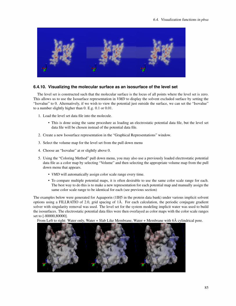
6.4. Visualization functions in pbsa
6.4.10. Visualizing the molecular surface as an isosurface of the level set
The level set is constructed such that the molecular surface is the locus of all points where the level set is zero.This allows us to use the Isosurface representation in VMD to display the solvent excluded surface by setting the“Isovalue” to 0. Alternatively, if we wish to view the potential just outside the surface, we can set the “Isovalue”to a number slightly higher than 0. E.g. 0.1 or 0.01.
1. Load the level set data file into the molecule.
• This is done using the same procedure as loading an electrostatic potential data file, but the level setdata file will be chosen instead of the potential data file.
2. Create a new Isosurface representation in the “Graphical Representations” window.
3. Select the volume map for the level set from the pull down menu
4. Choose an “Isovalue” at or slightly above 0.
5. Using the “Coloring Method” pull down menu, you may also use a previously loaded electrostatic potentialdata file as a color map by selecting “Volume” and then selecting the appropriate volume map from the pulldown menu that appears.
• VMD will automatically assign color scale range every time.
• To compare multiple potential maps, it is often desirable to use the same color scale range for each.The best way to do this is to make a new representation for each potential map and manually assign thesame color scale range to be identical for each (see previous section)
The examples below were generated for Aquaporin (1IH5 in the protein data bank) under various implicit solventoptions using a FILLRATIO of 2.0, grid spacing of 1Å. For each calculation, the periodic conjugate gradientsolver with singularity removal was used. The level set for the system modeling implicit water was used to buildthe isosurfaces. The electrostatic potential data files were then overlayed as color maps with the color scale rangesset to [-80000,80000].
From Left to right: Water only, Water + Slab Like Membrane, Water + Membrane with 6Å cylindrical pore.
85

6. PBSA
6.4.11. Visualizing interior channels, voids, and solvent pockets
One of the common roles for membrane proteins is to act as a transmembrane channel, to allow specific sub-stance to pass from one side of a membrane to another. Features such as solvent / ion channels or internal voidswill often be occluded from view by the exterior surface. One option that can allow these to be viewed is to usethe clipping plane tool in VMD.
1. Open the “Exensions” pull down menu in the “VMD Main” window and go to the “Visualization” submenuand select “Clipping Plane Tool”.
2. The “Clip Tool” window should pop up.
3. The “Distance” slider allows clipping to be set
4. The “Normal” slider sets the normal of the clipping plane.
• The “flip” button on the right will let you clip from front to back, which will be useful to clip theoccluding exteriro surface from the view and reveal the interior.
The clipping tool was used to reveal the internal pore region for the aquaporin system setups used in the previoussection.
From Left to right: Water only, Water + Slab like Membrane, Water + Membrane with pore region excluded.
As an alternative, the level set map generated using PORTYPE=1 with the implicit membrane option will allowa cylindrical region to be excluded from the membrane level set. The corresponding isosurface will show anyinterior cavities or voids which fall within this region for isovalues at or slightly above 0 (since the level set at themembrane-solute interface will be below 0). See the previous section for details on writing and loading the levelset file.
Shown below is the level set isosurface for the aquaporin system with implicit water plus a membrane with acylindrical region removed. The corresponding potential data was again overlayed as a color map. The surface ofthe channel region, and the membrane-solvent interface planes are now clearly visible.
6.4.12. Importing / Modifying Atomic Radii to VMD from the prmtop file
Currently, VMD does not support loading radii for atoms directly from the prmtop file when it loads a molecule.These values can be loaded relatively easily using the tkconsole, however. To do so:
86

6.5. pbsa in sander and NAB
1. select “Tk Console” from the “Extensions” menu in the “VMD Main” window.
• The “VMD TkConsole” window will then open
2. Be sure that the atom you want to import radii for is the top molecule on the list in the VMD Main window.If it is not, you will need to replace “top” with the appropriate ID
3. Type or copy and paste the following lines, but DO NOT hit enter yet.
set prot [atomselect “top” all]
$prot set radius #RadiiList#
4. You will now need to replace #RadiiList# with the one from the prmtop file.
a) Open the prmtop file for the molecule using a text editor
b) find the section that starts with “%FLAG RADII”
c) Highlight/Select the list of numbers that follows “%FORMAT(5E16.8)”
d) Copy the list (usually done by selecting “Copy” from the “Edit” menu in your text editor)
e) Go back to the “VMD TkConsole” window
f) Highlight/Select #RadiiList#
g) Select “Paste Ctrl-v” from the “Edit” menu in the “VMD TkConsole” window
5. Now hit return
• If this was successful, you should now have the correct radii for each atom in the molecule.
• you can have the console print the list of all radii by typing:
$prot get radius
• For a more human readable printout, use:
for set ind 0 $ind<[llength $rad] incr ind \
puts "Atom $ind radius is [lindex $rad $ind]"
These radii are used by VMD to display the VDW surface (made by selecting “VDW” from the “DrawingMethod” pull down menu in the “Graphical Representations” window). One useful trick is to set them to be asmall amount larger (say .01 Å) than those used to generate the surface. This will ensure that the color map willrepresent the external field just outside of the molecule. To modify the radii type or copy the following in the TkConsole:
set rad [$prot get radius]
for set ind 0 $ind<[llength $rad] incr ind \
lset rad $ind [expr [lindex $rad $ind] +.01]
The above code will increase all atomic radii by .01 angstroms. This can be changed if a different amount isdesired. (The code assumes you already followed steps 1 through 5 otherwise $prot will be undefined!)
6.5. pbsa in sander and NAB
6.5.1. Electrostatic forces/gradients in pbsa
Force calculation in the finite-difference Poisson-Boltzmann method is straightforward, though not a trivialissue. It can be shown, by using the variation of the electrostatic free energy, that the electrostatic force densityconsists of three components, viz., the reaction field force, the dielectric boundary force, and the ionic force. [186]Since the ionic force is much smaller in absolute value than the other two components, we only include the reactionfield force and the dielectric boundary force in this release.
87

6. PBSA
The reaction field force only exists where there are atomic charges, so that it is straightforward to be mappedonto atoms. In contrast, the dielectric boundary force exists on the molecular surface where the dielectric constantchanges. The surface force, or pressure, cannot be easily mapped onto atoms. This is because a force-mappingprocedure from the molecular surface to atoms apparently needs the derivatives of molecular surface with respectto atomic positions. However such derivatives do not exist for the widely used molecular surface definition, i.e.,the solvent excluded surface (SES). We are actively developing an analytical molecular surface definition that isconsistent with the widely used SES definition for the numerical PB methods so that this difficulty will be overcomein future releases.
Temporarily, a partial solution in the mapping of dielectric boundary force as described by Gilson et al[186]is implemented for PB dynamics and minimization when the SES definition is used. The stability of the MDsimulation has been much improved with a more accurate mapping method of analytical SES.
6.5.2. Example for pbsa in sander
All pbsa functionalities are available in sander and all input options are exactly the same as in the standalonepbsa. An apparent exception is IPB: you need to really set IPB to nonzero in order to invoke pbsa functionalities.All other default values of PB options in sander are same as those in pbsa for single point calculations, whereasthere are some options that have different recommended or default values when PB minimization or dynamics isenabled. These options are
space=0.25
arcres=0.125
fscale=4
eneopt=2
bcopt=6
frcopt=2
The SPACE, ARCRES and FSCALE are all set for higher resolution of the grid so that the force calculation canbe more accurate. The charge view method (ENEOPT = 2, FRCOPT = 2) is used here because it has been testedto be able to run stable molecular dynamics simulations. Plus, BCOPT is set to 6 to remove charge singularity forthe same stability purpose. An example input for PBMD is given as follows
Sample PB visualization input
&cntrl
imin=0, ntx=1, irest=0,
ipb=2, ntb=0,
ntc=2, ntf=2,
tempi=100, temp0=100, ntt=3, gamma_ln=1,
nstlim=100000, dt=0.002,
ntpr=100, ntwr=100000, ntwx=100,
/
&pb
npbgrid=500, nsnba=5,
/
IPB is explicitly set to 2 to enable PB dynamics. The NPBGRID option is set to 500, which means the finitedifference grid is regenerated every 500 dynamics steps. NSNBA = 5 means the atom-based pairlist is generatedevery 5 steps. Please refer to Chapter 18 for the other &cntrl options. Note that the above input can be used withsander only.
6.5.3. Example for pbsa in NAB
pbsa functionalities are available in NAB as a part of the standard build. However the available input optionsare limited, please refer to the table in Section 40.1 for the list of available pbsa input options. The structures and
88

6.5. pbsa in sander and NAB
parameters are supplied by NAB’s facility. Here is a sample of calls in a NAB program to the mm_options()routine, in order to run pbsa:
mm_options("ntpr=1, cut=99.0"); // No solute-solute cutoff
mm_options("ipb=2"); // Use PBSA
mm_options("accept=0.000001"); // Convergence criterion
mm_options("dprob=1.6"); // Solvent probe radius for SASA
mm_options("radiopt=1"); // Useatom-type/charge-based radii
mm_options("fillratio=4"); // Coarse/Fine ratio of electrostatic focusing
89

7. Reference Interaction Site Model
In addition to explicit and continuum implicit solvation models, Amber also has a third type of solvation modelfor molecular mechanics simulations, the reference interaction site model (RISM) of molecular solvation[187–200]. In AmberTools, 1D-RISM is available as rism1d. 3D-RISM is available as an option in NAB, MMPBSA.pyand sander. rism3d.snglpnt is a simplified, standalone interface, ideal for calculating solvation thermodynamics onindividual structures and trajectories. Details specific to using sander and sander.MPI can be found in Chapter 18.
7.1. Introduction
RISM is an inherently microscopic approach, calculating the equilibrium distribution of the solvent, from whichall thermodynamic properties are then arrived at. Specifically, RISM is an approximate solution to the Ornstein-Zernike (OZ) equation[188, 197, 198, 201, 202]
h(r12,Ω1,Ω2) = c(r12,Ω1,Ω2)+ρ
∫dr3 dΩ3 c(r13,Ω1,Ω3)h(r32,Ω3,Ω2), (7.1)
where r12 is the separation between particles 1 and 2 while Ω1 and Ω2 are their orientations relative to the vectorr12. The two functions in this relation are h, the total correlation function, and c, the direct correlation function.The total correlation function is defined as
hab(rab,Ωa,Ωb)≡ gab(rab,Ωa,Ωb)−1,
where gab is the pair-distribution function, which gives the conditional density distribution of species b about a. Incases where only radial separation is considered, for example by orientational averaging over site α of species aand site γ of species b, gives the familiar one dimensional site-site radial distribution function, gαγ(rαγ).
For real mixtures, it is often convenient to speak in terms of a solvent, V, of high concentration and a solute, U,of low concentration. A generic case of solvation is infinite dilution of the solute, i.e., ρU → 0. We can rewriteEquation (7.1), in the limit of infinite dilution, as a set of three equations:
hVV(r12,Ω1,Ω2) = cVV(r12,Ω1,Ω2)+ρV∫
dr3 dΩ3 cVV(r13,Ω1,Ω3)hVV(r32,Ω3,Ω2), (7.2)
hUV(r12,Ω1,Ω2) = cUV(r12,Ω1,Ω2)+ρV∫
dr3 dΩ3 cUV(r13,Ω1,Ω3)hVV(r32,Ω3,Ω2), (7.3)
hUU(r12,Ω1,Ω2) = cUU(r12,Ω1,Ω2)+ρV∫
dr3 dΩ3 cUV(r13,Ω1,Ω3)hVU(r32,Ω3,Ω2). (7.4)
Equation (7.3) is directly relevant for biomolecular simulations where we are often interested in the properties ofa single, arbitrarily complex solute in the solution phase. Solutions to Equation (7.3) can be obtained using 3D-RISM. However, a solution to Equation (7.2) for pure solvent is a necessary prerequisite and is readily obtainedfrom 1D-RISM.
To obtain a solution to the OZ equations it is necessary to have a second equation that relates h and c or uniquelydefines one of these functions. The general closure relation is[201]
g(r12,Ω1,Ω2) = exp [−βu(r12,Ω1,Ω2)+h(r12,Ω1,Ω2)− c(r12,Ω1,Ω2)+b(r12,Ω1,Ω2)] (7.5)
u is the potential energy function for the two particles and b is known as the bridge function (a non-local functional,representable as infinite diagrammatic series in terms of h [201]). It should be noted that u is the only point atwhich the interaction potential enters the equations. Depending on the method used to solve the OZ equations, u
90
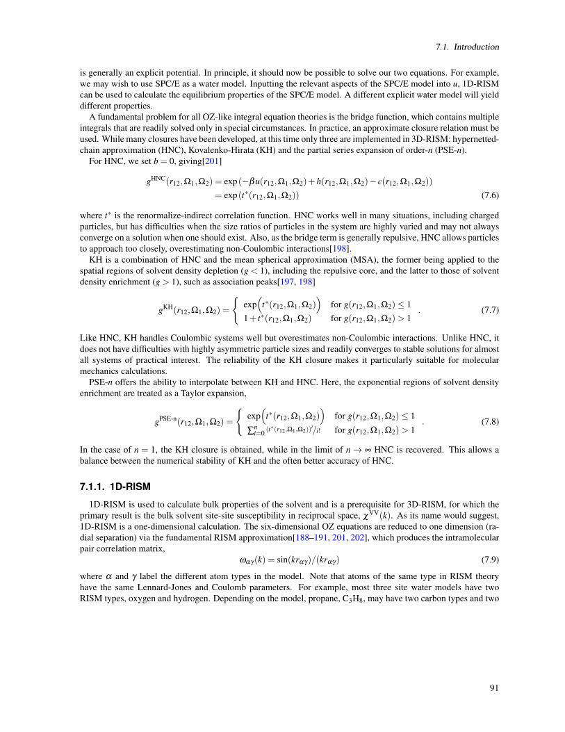
7.1. Introduction
is generally an explicit potential. In principle, it should now be possible to solve our two equations. For example,we may wish to use SPC/E as a water model. Inputting the relevant aspects of the SPC/E model into u, 1D-RISMcan be used to calculate the equilibrium properties of the SPC/E model. A different explicit water model will yielddifferent properties.
A fundamental problem for all OZ-like integral equation theories is the bridge function, which contains multipleintegrals that are readily solved only in special circumstances. In practice, an approximate closure relation must beused. While many closures have been developed, at this time only three are implemented in 3D-RISM: hypernetted-chain approximation (HNC), Kovalenko-Hirata (KH) and the partial series expansion of order-n (PSE-n).
For HNC, we set b = 0, giving[201]
gHNC(r12,Ω1,Ω2) = exp(−βu(r12,Ω1,Ω2)+h(r12,Ω1,Ω2)− c(r12,Ω1,Ω2))
= exp(t∗(r12,Ω1,Ω2)) (7.6)
where t∗ is the renormalize-indirect correlation function. HNC works well in many situations, including chargedparticles, but has difficulties when the size ratios of particles in the system are highly varied and may not alwaysconverge on a solution when one should exist. Also, as the bridge term is generally repulsive, HNC allows particlesto approach too closely, overestimating non-Coulombic interactions[198].
KH is a combination of HNC and the mean spherical approximation (MSA), the former being applied to thespatial regions of solvent density depletion (g < 1), including the repulsive core, and the latter to those of solventdensity enrichment (g > 1), such as association peaks[197, 198]
gKH(r12,Ω1,Ω2) =
exp(
t∗(r12,Ω1,Ω2))
for g(r12,Ω1,Ω2)≤ 11+ t∗(r12,Ω1,Ω2) for g(r12,Ω1,Ω2)> 1
. (7.7)
Like HNC, KH handles Coulombic systems well but overestimates non-Coulombic interactions. Unlike HNC, itdoes not have difficulties with highly asymmetric particle sizes and readily converges to stable solutions for almostall systems of practical interest. The reliability of the KH closure makes it particularly suitable for molecularmechanics calculations.
PSE-n offers the ability to interpolate between KH and HNC. Here, the exponential regions of solvent densityenrichment are treated as a Taylor expansion,
gPSE-n(r12,Ω1,Ω2) =
exp(
t∗(r12,Ω1,Ω2))
for g(r12,Ω1,Ω2)≤ 1
∑ni=0 (t∗(r12,Ω1,Ω2))
i/i! for g(r12,Ω1,Ω2)> 1. (7.8)
In the case of n = 1, the KH closure is obtained, while in the limit of n→ ∞ HNC is recovered. This allows abalance between the numerical stability of KH and the often better accuracy of HNC.
7.1.1. 1D-RISM
1D-RISM is used to calculate bulk properties of the solvent and is a prerequisite for 3D-RISM, for which theprimary result is the bulk solvent site-site susceptibility in reciprocal space, χVV(k). As its name would suggest,1D-RISM is a one-dimensional calculation. The six-dimensional OZ equations are reduced to one dimension (ra-dial separation) via the fundamental RISM approximation[188–191, 201, 202], which produces the intramolecularpair correlation matrix,
ωαγ(k) = sin(krαγ)/(krαγ) (7.9)
where α and γ label the different atom types in the model. Note that atoms of the same type in RISM theoryhave the same Lennard-Jones and Coulomb parameters. For example, most three site water models have twoRISM types, oxygen and hydrogen. Depending on the model, propane, C3H8, may have two carbon types and two
91
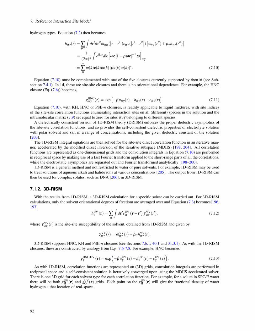
7. Reference Interaction Site Model
hydrogen types. Equation (7.2) then becomes
hαγ(r) = ∑µν
∫dr′dr′′ωαµ(
∣∣r− r′∣∣)cµν(
∣∣r′− r′′∣∣)[ωνγ(r′′)+ρν hνγ(r′′)
]=
1(2π)3
∫eik·rdk
[ωc [1−ρωc]−1
ω
]αγ
=∞
∑0
ω(k)c(k)ω(k) [ρc(k)ω(k)]n . (7.10)
Equation (7.10) must be complemented with one of the five closures currently supported by rism1d (see Sub-section 7.4.1). In 1d, these are site-site closures and there is no orientational dependence. For example, the HNCclosure (Eq. (7.6)) becomes,
gHNCαγ (r) = exp
[−βuαγ(r)+hαγ(r)− cαγ(r)
]. (7.11)
Equation (7.10), with KH, HNC or PSE-n closures, is readily applicable to liquid mixtures, with site indicesof the site-site correlation functions enumerating interaction sites on all (different) species in the solution and theintramolecular matrix (7.9) set equal to zero for sites α,γ belonging to different species.
A dielectrically consistent version of 1D-RISM theory (DRISM) enforces the proper dielectric asymptotics ofthe site-site correlation functions, and so provides the self-consistent dielectric properties of electrolyte solutionwith polar solvent and salt in a range of concentrations, including the given dielectric constant of the solution[203].
The 1D-RISM integral equations are then solved for the site-site direct correlation function in an iterative man-ner, accelerated by the modified direct inversion of the iterative subspace (MDIIS) [198, 204]. All correlationfunctions are represented as one-dimensional grids and the convolution integrals in Equation (7.10) are performedin reciprocal space by making use of a fast Fourier transform applied to the short-range parts of all the correlations,while the electrostatic asymptotics are separated out and Fourier transformed analytically [198–200].
1D-RISM is a general method and not restricted to water or pure solvents. For example, 1D-RISM may be usedto treat solutions of aqueous alkali and halide ions at various concentrations [205]. The output from 1D-RISM canthen be used for complex solutes, such as DNA [206], in 3D-RISM.
7.1.2. 3D-RISM
With the results from 1D-RISM, a 3D-RISM calculation for a specific solute can be carried out. For 3D-RISMcalculations, only the solvent orientational degrees of freedom are averaged over and Equation (7.3) becomes[196,197]
hUVγ (r) = ∑
α
∫dr′cUV
α
(r− r′
)χ
VVαγ (r′), (7.12)
where χVVαγ (r) is the site-site susceptibility of the solvent, obtained from 1D-RISM and given by
χVVαγ (r) = ω
VVαγ (r)+ρα hVV
αγ (r).
3D-RISM supports HNC, KH and PSE-n closures (see Sections 7.6.1, 40.1 and 31.3.1). As with the 1D-RISMclosures, these are constructed by analogy from Eqs. 7.6-7.8. For example, HNC becomes
gHNC,UVγ (r) = exp
(−βuUV
γ (r)+hUVγ (r)− cUV
γ (r)). (7.13)
As with 1D-RISM, correlation functions are represented on (3D) grids, convolution integrals are performed inreciprocal space and a self-consistent solution is iteratively converged upon using the MDIIS accelerated solver.There is one 3D grid for each solvent type for each correlation function. For example, for a solute in SPC/E waterthere will be both gUV
H (r) and gUVO (r) grids. Each point on the gUV
H (r) will give the fractional density of waterhydrogen a that location of real-space.
92

7.1. Introduction
To properly treat electrostatic forces in electrolyte solution with polar molecular solvent and ionic species, theelectrostatic asymptotics of all the correlation functions (both the 3D and radial ones) are treated analytically [198,199, 207]. The non-periodic electrostatic asymptotics are separated out in the direct and reciprocal space and theremaining short-range terms of the correlation functions are discretized on a 3D grid in a non-periodic box largeenough to ensure decay of the short-range terms at the box boundaries [207]. The convolution of the short-rangeterms in the integral equation (7.12) is calculated using 3D fast Fourier transform [208, 209]. Accordingly, theelectrostatic asymptotics terms in the thermodynamics integral (7.15) below are handled analytically and reducedto one-dimensional integrals easy to compute [207].
With a converged 3D-RISM solution for hUV and cUV, it is straightforward to calculate solvation thermody-namics. From the perspective of molecular simulations, the most important thermodynamic values are the excesschemical potential of solvation (solvation free energy), µex and the mean solvation force, fUV
i (Ri), on each soluteatom, i. µex can be obtained through analytical thermodynamic integration for HNC,
µex,HNC = kBT ∑
α
ρVα
∫dr[
12(hUV
α (r))2− cUV
α (r)− 12
hUVα (r)cUV
α (r)], (7.14)
KH ,
µex,KH = kBT ∑
α
ρVα
∫dr[
12(hUV
α (r))2
Θ(−hUV
α (r))− cUV
α (r)− 12
hUVα (r)cUV
α (r)], (7.15)
and PSE-n,
µex,PSE-n = kBT ∑
α
ρVα
∫dr[
12(hUV
α (r))2− cUV
α (r)− 12
hUVα (r)cUV
α (r)
− (t∗ (r))n+1
(n+1)!Θ(hUV
α (r))]
, (7.16)
where Θ is the Heaviside function.Analogous versions of Eqns. 7.6, 7.15 and 7.16 are used in 1D-RISM. While these are used for DRISM they
are have been derived for XRISM. Furthermore, these equations have been derived a number of different wayswith slightly different functional forms of the − 1
2 hc term [197, 210–213]. These different functional forms areequivalent in XRISM but not in DRISM. The form introduced by Pettitt and Rossky [211] is the most popularin the literature and the default selection in rism1d. It is possible to have rism1d evaluate and output all threefunctional forms (see Output) but, for DRISM, none of these expressions are strictly correct.
The force equation
fUVi (Ri) =−
∂ µex
∂Ri=−∑
α
ρα
∫drgUV
α (r)∂uUV
α (r−Ri)
∂Ri
is valid for all closures with a path independent expression for the excess chemical potential, such as HNC, KHand PSE-n closures implemented in 3D-RISM [187, 214–216].
In addition to closure specific expressions for the solvation free energy, other approximations also exist. TheGaussian fluctuation (GF) approximation[217, 218] is given as
µex,GF = kBT ∑
α
ρVα
∫dr[−cUV
α (r)− 12
hUVα (r)cUV
α (r)]
(7.17)
and has been shown to yield improved absolute solvation free energies for both polar and non-polar solutes[218,219] but not necessarily for relative free energies[220]. It is not associated with a particular closure but is typicallyused in place of the expression for a given closure.
Eqs. (7.14)-(7.16) give the total solvation free energy, ∆Gsol, but it is often useful to decompose this into elec-trostatic (solvent polarization), ∆Gpol, and non-electrostatic (dispersion and cavity formation), (∆Gdis +∆Gcav),terms. Conceptually, we can divide the path of the thermodynamic integration into two steps: first the solutewithout partial charges is inserted into the solvent (dispersion and cavity formation) and then partial charges are
93

7. Reference Interaction Site Model
introduced, which polarize the solvent,
µex = ∆Gsol = ∆Gpol +∆Gdis +∆Gcav.
∆Gsol is produced by a 3D-RISM calculation on the charged solute. ∆Gpol is then the difference of the twocalculations. As a point of reference, generalized-Born and Poisson-Boltzmann methods calculate only ∆Gpol and,typically, use a calculation involving solvent accessible surface area to predict ∆Gdis +∆Gcav.
7.1.3. Analytic Temperature Derivatives
For the thermodynamic analysis of solvation, it is often useful to calculate the energetic and entropic contribu-tions, εsolvand−T Ssolv respectively, to the solvation free energy. It has been shown that it is possible to analyticallydecompose the solvation free energy into these two contributions when the solvation free energy has a closed ana-lytical form, such as with HNC and KH closure [221]. In what follows, the analytical expression of energetic andentropic contributions to the solvation free energy are derived in the framework of 1D-RISM theory with HNCclosure. The similar derivation can be applied to other closures as well as to the framework of 3D-RISM theory.At this time, temperature derivatives are implemented for with HNC, KH and PSE-n closures in both 1D- and3D-RISM [222].
The solvation free energy of species U in a solution consisting of N total species is expressed in the RISM-HNCframework as
µex,UHNC = kBT ∑
on Uα ∑
NM=1 ∑
on Mγ ργ
∫dr[
12
(hαγ(r)
)2− cαγ(r)− 12 hαγ(r)cαγ(r)
].
The differentiation of the solvation free energy with respect to the temperature T leads to
δT µex,UHNC =
µex,UHNC + kBT ∑
on Uα ∑
NM=1 ∑
on Mγ ργ
∫dr
[hαγ(r) ·δT hαγ(r)−δT cαγ(r)− 1
2 δT hαγ(r) · cαγ(r)− 12 hαγ(r) ·δT cαγ(r)
].
where δT is T ∂
∂T . Since µex,UHNC = εsolv,U −T Ssolv,U , we have δT µ
ex,UHNC =−T Ssolv,U and therefore the above equation
can be rearranged as
εsolv,U =
−kBT ∑on Uα ∑
NM=1 ∑
on Mγ ργ
∫dr
[hαγ(r) ·δT hαγ(r)−δT cαγ(r)− 1
2 δT hαγ(r) · cαγ(r)− 12 hαγ(r) ·δT cαγ(r)
].
It is noted that the solvation energy εsolv,U can be viewed as consisting of two contributions: one arising fromcreation of a polarized cavity (in pure solvent) and the other corresponding to the energy of embedding the solutemolecule into the cavity. The former is the solvent reorganization energy and the latter is the averagesolute-solvent interaction energy that is obtained as ∑α ∑γ ργ
∫druαγ gαγ .
The temperature derivatives of correlation functionsδT h(r) and δT c(r) can be obtained by solving the tempera-ture derivative of RISM-HNC equations
δT h(k) = w(k)δT c(k)w(k)+ρw(k)δT c(k)h(k)+ρw(k)c(k)δT h(k)
and
δT hαγ(r) =[
uαγ (r)kBT +δT hαγ(r)−δT cαγ(r)
](hαγ(r)+1).
Some practical examples can be found in [223], [224] and [222].
94

7.2. Practical Considerations
7.2. Practical Considerations
7.2.1. Computational Requirements and Parallel Scaling
Calculating a 3D-RISM solution for a single solute conformation typically requires about 100 times more com-puter time than the same calculation with explicit solvent or PB. While there are other factors to consider, such assampling confined solvent or overall efficiency of sampling in the whole statistical ensemble at once, this can beprohibitive for many applications. Memory is also an issue as the 3D correlation grids require anywhere from afew megabytes for the smallest solutes to gigabytes for large complexes. A lower bound and very good estimatefor the total memory required is
Total memory≥ 8bytes×
Nbox NV
2NMDIIS︸ ︷︷ ︸c,residual
+ 1︸︷︷︸u
+ Ndecomp︸ ︷︷ ︸polar decomp
Npropagate︸ ︷︷ ︸past solutions
(Nbox +2NyNz)
4︸︷︷︸asymptotics
+ 1︸︷︷︸FFT scratch
+ 2︸︷︷︸g,h
NV
where Nbox = Nx×Ny×Nz is the total number of grid points, NV is the number of solvent atom species and NMDIISis the number of MDIIS vectors used to accelerate convergence. uUV, cUV and the residual of cUV are stored inreal-space only and require a full grid for each solvent. cUV and its residual also require NMDIIS grids for theMDIIS routine (see the mdiis_nvec keyword) and Npropagate grids to make use of solutions from previous soluteconfigurations to improve the initial guess (see the npropagate keyword). If a polar/non-polar decomposition isrequested (see the polardecomp keyword) an additional set of grids for past solutions with no solute charges iskept (Ndecomp = 2); by default this is turned off (Ndecomp = 1). The full real space grid plus an additional 2NyNxgrid points are needed (due to the FFT) for g and h for each solvent species and for the four grids requiredto compute the long range asymptotics. Memory, therefore, scales linearly with Nbox while computation timescales as O(Nbox log(Nbox)) due to the requirements of calculating the 3D fast Fourier transform (3D-FFT). Toovercome these requirements, two options are available beyond optimizations already in place, multiple time stepsand parallelization. Multiple time step methods are available only in sander (Chapter 18) and are applicable tomolecular dynamics calculations only. Parallelization is available for all calculations but is limited by system sizeand computational resources.
Both sander and NAB have MPI implementations of 3D-RISM (see Section 7.5.5 for NAB compiling instruc-tions) that distribute both memory requirements and computational load. As memory is distributed, the aggregatememory of many computers can be used to perform calculations on very large systems. Memory distribution ishandled by the FFTW 3.3 library so decomposition is done along the z-axis. If a variable solvation box size isused, the only consideration is to avoid specifying a large, prime number of processes (≥ 7). For fixed box sizes,the number of grids points in each dimension must be divisible by two (a general requirement) and the numberof grid points in the z-axis must be divisible by the number of processes. sander.MPI also has the additionalconsideration that the number of processes cannot be larger than the number of solute residues; NAB does not sufferfrom this limitation.
7.2.2. Output
gUV, hUV and cUV files can be output for 3D-RISM calculations and are useful for visualization and calculation ofthermodynamic quantities. These use the ASCII Data Explorer (DX) file format (See http://ambermd.org/formats.html)so there is one file for each solvent atom type for each requested frame. Each file is
(348+Nbox×16 1
3
)bytes,
which can quickly fill disk space. Also, very few visualization programs are capable of displaying both molecularand volumetric trajectories.
95

7. Reference Interaction Site Model
7.2.3. Numerical Accuracy
Numerical accuracy depends on the specified residual tolerance for the solution and the solvation box physicalsize and grid spacing. Almost all applications should use a grid spacing of 0.5 Å. A larger grid spacing quickly leadsto severe errors in thermodynamic quantities. Smaller grid spacing may be necessary for some applications (e.g.,mapping potentials of mean force) but this is rare and computationally expensive. A buffer distance between thesolute and the edges of the solvent box should typically be at least 14 Å for water or larger for ionic solutions. Thesolvation box size should be increased until the thermodynamic properties converge (see Section 7.5.1). Moleculardynamics[187], minimization and trajectory post-processing[220] have different requirements for the maximumresidual tolerance. Molecular dynamics does well with a tolerance of 10−5 and npropagate=5. Minimizationrequires tolerances of 10−11 or lower and is typically limited to drms ≥ 10−4. Trajectory post-processing forMM/RISM type calculations typically have high statistical noise from the trajectory itself and it is possible to usea tolerance of 10−3 and npropagate=1. However, this should be compared against a tolerance of 10−5 on a subsetof the data before committing to this level of accuracy.
7.2.4. Solvation Free Energy Corrections
3D-RISM with HNC-like closures is known to overestimate the non-polar component of the solvation freeenergy. Several alternate expressions for the solvation free energy have been developed to correct this and are basedall, or in part, on the partial molar volume (PMV) of the solute. These include the Universal Correction (UC) [225],Ng Bridge Correction (NgB) [226] and the Pressure Correction Plus (PC+/3D-RISM) correction [227]. 3D-RISMcurrently implements UC and PV+/3D-RISM as runtime options. NgB results can be calculated from the standardthermodynamic output if the polarDecomp option is used but is not implemented directly. UC and NgB are bothparameterized corrections. So, parameters for these corrections must be used only with the .xvv file used to createthem. Our implementation of UC uses the excess chemical potential of the closure rather than the GF functional,as we have found this provides better results in general [222]. All of these corrections have been almost exclusivelyused with pure water under ambient conditions, though there are promising results for UC with non-polar liquids.Using these methods with different solvents and co-solvents is a subject of on-going research.
7.3. Work Flow
Using 3D-RISM with SANDER or NAB for molecular dynamics, minimization or snapshot analysis is verysimilar to using implicit solvent models like GBSA or PBSA. However, some additional preliminary setup isrequired, the extent of which depends on the solvent to be used.
3D-RISM requires detailed information of the bulk solvent in the form of the site-site susceptibility, χVV, andproperties such as the temperature and partial charges. This is read in as an .xvv file, which is produced by a1D-RISM calculation. If another 3D-RISM calculation is to be preformed with any details of the bulk solventchanged (e.g., temperature or pressure) a new .xvv file must be produced. Examples of precomputed .xvv filesfor SPC/E and TIP3P water can be found in $AMBERHOME/AmberTools/test/rism1d.
Special care must be taken when producing .xvv files for use with 3D-RISM, particularly with respect to gridparameters. It is important that the spatial extent of the grid be large enough to capture the essential long rangefeatures of the solvent while the spacing must be fine enough to sample the short-range structure. A grid spacingof 0.025 Å is sufficient for most applications. The number of grid points required, which will determine thephysical length of the grid in Å, generally depends on the properties of the solvent. Low concentration aqueoussalt solutions typically require much larger grids than pure bulk water. A good indicator that the grid is largeenough is convergence of delhv0 in the .xvv file. When converged, delhv0 should retain four to five digits ofprecision when the number of grid points is doubled.
The ability of 3D-RISM to perform temperature derivatives and calculate solvation energy and entropy requires.xvv files with with temperature dependence information. rism1d must be run with entropicDecomp option turnedon (Section 7.4.1). The version number in the .xvv file header indicates the maximum information available. Ver-sion 1.001 (current) allows temperature derivatives and solvation entropies and energies for all reported quantities.Version 1.000 (since Amber12) does not allow temperature derivatives of the PMV or solventation energies andentropies of PMV-based corrections. Version 0.001 does not have information for any temperature derivatives.
96

7.3. Work Flow
1D-RISM calculations require details of the some bulk properties of the solvent, such as temperature and di-electric constant, and an explicit model of the molecular components. These are read in from one or more .mdl
files, depending on the composition of the solvent. Several .mdl files are included in the Amber11 distributionand can be found in $AMBERHOME/dat/rism1d/model. These include many of the explicit models for solvent andions used with the Amber force fields. Other solvents models may be used by creating appropriate MDL files. SeeSection 7.8 for format details.
7.3.1. Solution Convergence
The default parameters for 3D-RISM are selected to provide the best performance for the majority of systems.In cases where a convergence is not achieved, the strategies below may be useful.
7.3.1.1. Closure Bootstrap
When a PSE-n or HNC closure is desired, the most effective method to overcome convergence issues is to usea low order closure solution as a starting guess. The KH closure should be the starting point as it is numericallyrobust and, typically, converges easily in the vast majority of case. After this, higher orders of PSE-n can be useduntil the desired closure is reached. The procedure for 1D-RISM and 3D-RISM differs slightly in practice.
1D-RISM rism1d can use restart files to implement this approach (see Section Subsection 7.4.1). First, runrism1d with the KH closure to convergence. Then use the .sav file as input for the next highest closure. The rootname of the .sav file must be the same as your .inp file. To avoid overwriting lower order solutions, name the filesby closure or use separate directories. You will have to rename the .sav files as you go.
3D-RISM All 3D-RISM interfaces have closure bootstrapping builtin via the closure and tolerance keywords.Closures should be specified as an ordered list with last closure being the highest order closure. The solutions ofthe intermediate closures can have a high tolerance. The default tolerance for intermediate closures is 1 and thereis no observed benefit to tolerances less than 1e-2. See details in Subsection 7.6.1, Subsection 7.7.2.1 and Section40.1.
7.3.1.2. MDIIS Settings
MDIIS default setting are appropriate for most cases. Should your residual diverge or the solver get stuck on aparticular value, you can try modest adjustments.
Decrease mdiis_del mdiis_del controls the step size of MDIIS. A smaller step size can help convergence but ifthis is set too small it can cause convergence problems. For rism1d, this should be no lower than 0.1 or 0.2. For3D-RISM, it should be 0.5 at the lowest.
Increase mdiis_nvec This is the number of trial solutions that are saved for predicting a new solution. Theoptimal number for rapid convergence is typically 10 for 3D-RISM and 20 for 1D-RISM. However, for 3D-RISM,the default choice of 5 requires much less memory and is computationally faster even though more iterations arerequired. Increasing the mdiis_nvec may help for 3D-RISM but is unlikely to help for 1D-RISM.
Increase mdiis_restart Occasionally, the MDIIS routine goes in the wrong direction and the residual increasessignificantly. If it increases more than mdiis_restart then the MDIIS routine selects the solution with the lowestresidual and purges the other trial solutions. The default value of 10 can be too aggressive and cause the solver tocycle. Increasing the value to 100 or 1000 sometimes allows the solver to recover from a misstep.
97
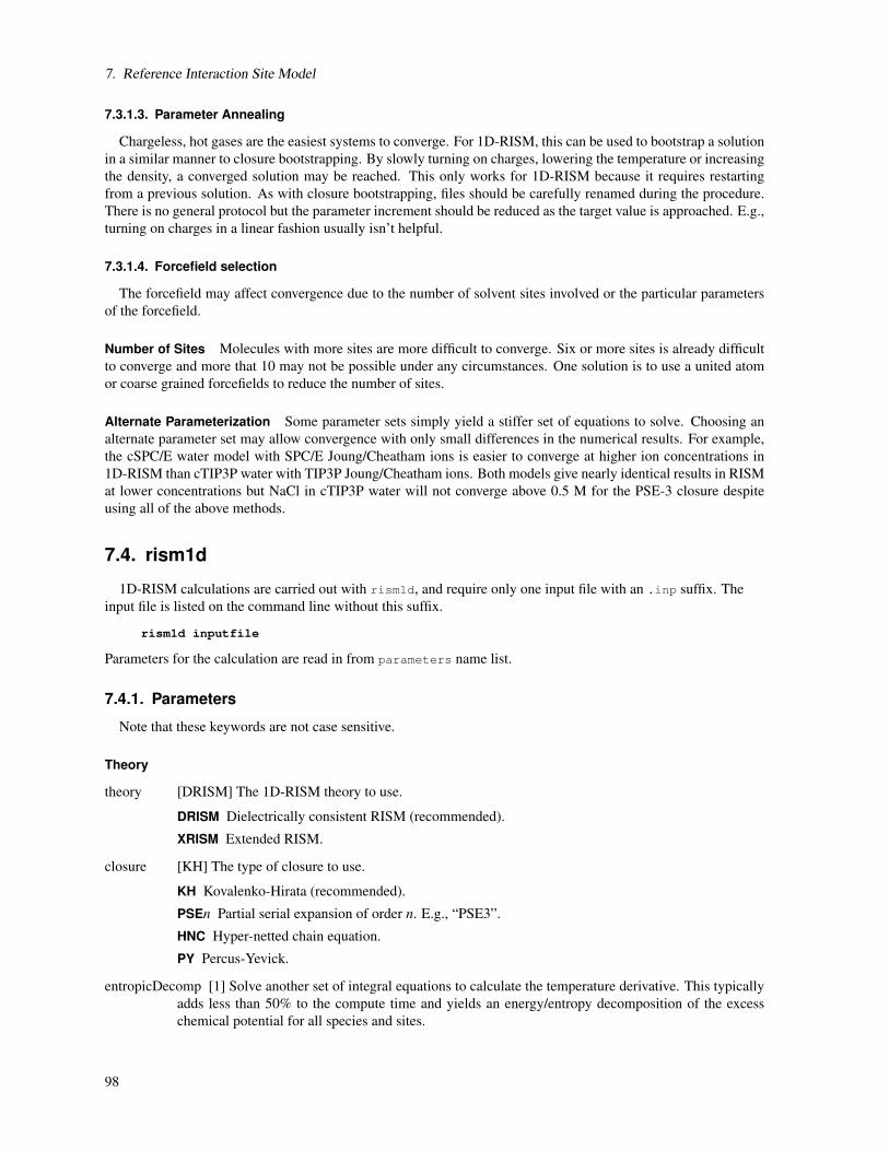
7. Reference Interaction Site Model
7.3.1.3. Parameter Annealing
Chargeless, hot gases are the easiest systems to converge. For 1D-RISM, this can be used to bootstrap a solutionin a similar manner to closure bootstrapping. By slowly turning on charges, lowering the temperature or increasingthe density, a converged solution may be reached. This only works for 1D-RISM because it requires restartingfrom a previous solution. As with closure bootstrapping, files should be carefully renamed during the procedure.There is no general protocol but the parameter increment should be reduced as the target value is approached. E.g.,turning on charges in a linear fashion usually isn’t helpful.
7.3.1.4. Forcefield selection
The forcefield may affect convergence due to the number of solvent sites involved or the particular parametersof the forcefield.
Number of Sites Molecules with more sites are more difficult to converge. Six or more sites is already difficultto converge and more that 10 may not be possible under any circumstances. One solution is to use a united atomor coarse grained forcefields to reduce the number of sites.
Alternate Parameterization Some parameter sets simply yield a stiffer set of equations to solve. Choosing analternate parameter set may allow convergence with only small differences in the numerical results. For example,the cSPC/E water model with SPC/E Joung/Cheatham ions is easier to converge at higher ion concentrations in1D-RISM than cTIP3P water with TIP3P Joung/Cheatham ions. Both models give nearly identical results in RISMat lower concentrations but NaCl in cTIP3P water will not converge above 0.5 M for the PSE-3 closure despiteusing all of the above methods.
7.4. rism1d
1D-RISM calculations are carried out with rism1d, and require only one input file with an .inp suffix. Theinput file is listed on the command line without this suffix.
rism1d inputfile
Parameters for the calculation are read in from parameters name list.
7.4.1. Parameters
Note that these keywords are not case sensitive.
Theory
theory [DRISM] The 1D-RISM theory to use.
DRISM Dielectrically consistent RISM (recommended).
XRISM Extended RISM.
closure [KH] The type of closure to use.
KH Kovalenko-Hirata (recommended).
PSEn Partial serial expansion of order n. E.g., “PSE3”.
HNC Hyper-netted chain equation.
PY Percus-Yevick.
entropicDecomp [1] Solve another set of integral equations to calculate the temperature derivative. This typicallyadds less than 50% to the compute time and yields an energy/entropy decomposition of the excesschemical potential for all species and sites.
98
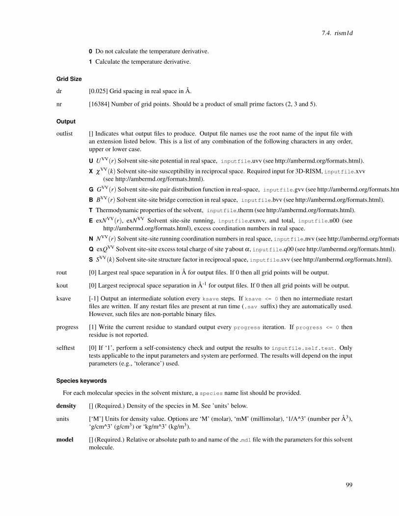
7.4. rism1d
0 Do not calculate the temperature derivative.
1 Calculate the temperature derivative.
Grid Size
dr [0.025] Grid spacing in real space in Å.
nr [16384] Number of grid points. Should be a product of small prime factors (2, 3 and 5).
Output
outlist [] Indicates what output files to produce. Output file names use the root name of the input file withan extension listed below. This is a list of any combination of the following characters in any order,upper or lower case.
U UVV(r) Solvent site-site potential in real space, inputfile.uvv (see http://ambermd.org/formats.html).
X χVV(k) Solvent site-site susceptibility in reciprocal space. Required input for 3D-RISM, inputfile.xvv(see http://ambermd.org/formats.html).
G GVV(r) Solvent site-site pair distribution function in real-space, inputfile.gvv (see http://ambermd.org/formats.html).
B BVV(r) Solvent site-site bridge correction in real space, inputfile.bvv (see http://ambermd.org/formats.html).
T Thermodynamic properties of the solvent, inputfile.therm (see http://ambermd.org/formats.html).
E exNVV(r), exNVV Solvent site-site running, inputfile.exnvv, and total, inputfile.n00 (seehttp://ambermd.org/formats.html), excess coordination numbers in real space.
N NVV(r) Solvent site-site running coordination numbers in real space, inputfile.nvv (see http://ambermd.org/formats.html).
Q exQVV Solvent site-site excess total charge of site γ about α , inputfile.q00 (see http://ambermd.org/formats.html).
S SVV(k) Solvent site-site structure factor in reciprocal space, inputfile.svv (see http://ambermd.org/formats.html).
rout [0] Largest real space separation in Å for output files. If 0 then all grid points will be output.
kout [0] Largest reciprocal space separation in Å-1 for output files. If 0 then all grid points will be output.
ksave [-1] Output an intermediate solution every ksave steps. If ksave <= 0 then no intermediate restartfiles are written. If any restart files are present at run time (.sav suffix) they are automatically used.However, such files are non-portable binary files.
progress [1] Write the current residue to standard output every progress iteration. If progress <= 0 thenresidue is not reported.
selftest [0] If ‘1’, perform a self-consistency check and output the results to inputfile.self.test. Onlytests applicable to the input parameters and system are performed. The results will depend on the inputparameters (e.g., ‘tolerance’) used.
Species keywords
For each molecular species in the solvent mixture, a species name list should be provided.
density [] (Required.) Density of the species in M. See ’units’ below.
units [‘M’] Units for density value. Options are ‘M’ (molar), ‘mM’ (millimolar), ‘1/A^3’ (number per Å3),‘g/cm^3’ (g/cm3) or ‘kg/m^3’ (kg/m3).
model [] (Required.) Relative or absolute path to and name of the .mdl file with the parameters for this solventmolecule.
99

7. Reference Interaction Site Model
Solution Convergence
rism1d uses MDIIS to accelerate convergence. The default parameters for this method are usually near optimalbut some systems can be difficult to converge. In such cases it may be useful to use a small step size (mdiis_del=0.1or 0.2). Occasionally, the target tolerance of 10−12 can not be achieved. A tolerance of 10−10 to 10−11 is oftensufficient but it is advisable to check how sensitive your calculations are to this.
mdiis_nvec [20] Number of MDIIS vectors to use.
mdiis_del [0.3] MDIIS step size.
mdiis_restart [10] If the current residual is mdiis_restart times larger than the smallest residual in memory,then the MDIIS procedure is restarted using the lowest residual solution stored in memory. Increasingthis number can sometimes help convergence.
tolerance [1e-12] Target residual tolerance for the self-consistent solution.
maxstep [10000] Maximum number of iterations to converge to a solution.
extra_precision [1] Controls the use of extra precision routines at key points in the 1D-RISM solver. This canbe useful for achieving low tolerances or for very large box lengths but increases computational cost.Strongly recommended for solutions with charged particles (e.g., salts).
0 No extra precision routines are used.
1 Sensitive matrix multiplication and addition routines are done in extra precision. A smallcomputational cost is incurred.
Solvent Description
temperature [298.15] Temperature in Kelvin.
dieps [] (Required.) Dielectric constant of the solvent.
nsp [] (Required.) Number of species (molecules) in the solutions. Also indicates the number of speciesname lists to follow.
Other
smear [1.0] Charge smear parameter in Å for long range asymptotics corrections.
adbcor [0.5] Numeric parameter for DRISM.
7.4.2. Example
Mixed ionic solvent.
&PARAMETERS
THEORY=’DRISM’, CLOSURE=’KH’, !Theory
NR=16384, DR=0.025, !Grid size and spacing
OUTLIST=’x’, ROUT=384, KOUT=0, !Output
MDIIS_NVEC=20, MDIIS_DEL=0.3, TOLERANCE=1.e-12, !MDIIS
KSAVE=-1, !Check pointing
PROGRESS=1, !Output frequency
MAXSTEP=10000, !Maximum iterations
SMEAR=1, ADBCOR=0.5, !Electrostatics
TEMPERATURE=310, DIEPS=78.497, NSP=3 !bulk solvent properties
/
&SPECIES
100

7.5. 3D-RISM in NAB
!SPC/E water
DENSITY=55.296d0, !very close to 0.0333 1/A3
MODEL="../../../dat/rism1d/model/SPC.mdl"
/
&SPECIES
!Sodium
units=’mM’
DENSITY=100,
MODEL="../../../dat/rism1d/model/Na+.mdl"
/
&SPECIES
!Chloride
units=’g/cm^3’
DENSITY=35.45e-4,
MODEL="../../../dat/rism1d/model/Cl-.mdl"
/
7.5. 3D-RISM in NAB
3D-RISM functionality is available in NAB and is built as part of the standard install procedure. MPI function-ality for 3D-RISM in NAB requires some additional information at compile time, described in Section 7.5.5. Atthis time, standard molecular dynamics and minimization with non-polarizable force fields are supported.
7.5.1. Solvation Box Size
The non-periodic solvation box super-cell can be defined as variable or fixed in size. When a variable box sizeis used, the box size will be adjusted to maintain a minimum buffer distance between the atoms of the solute andthe box boundary. This has the advantage of maintaining the smallest possible box size while adapting to changesof solute shape and orientation. Alternatively, the box size and grid spacing can be explicitly specified at run-timeand used for the duration of the calculation.
Regardless of how the solvation box is defined, the “center” of the solute is placed in the middle of the box. Thecenter of the solute and how it is placed in the solvent box is controlled with the centering keyword. Generally,centering=1 (center=center-of-mass) is the default and should be used for MD and centering=2 (center=center-of-geometry) should be used for minimization. Center-of-mass and center-of-geometry are conserved quantities ineach method respectively.
Other options for solute centering are available for special situations. To restrict the absolute position of grid-points to be integer multiples of the grid-spacing (e.g., (2.5 Å,3.0 Å) for a grid spacing of 0.5 Å) use centering=3for center-of-mass and centering=4 for center-of-geometry. To perform centering only on the first calculation (i.e.,first step of MD or minimization or first frame of a trajectory analysis), use the negative integer corresponding tothe desired center definition. This allows the solute to drift in the solvent box. Finally, with some care, it is possibleto achieve custom centering using centering=0. Here, no solute centering is performed and the solvent grid has anorigin of (0,0,0) and a center of ( x-length
2 + dx, y-length2 + dy, z-length
2 + dz). If you use centering=0, it is advisable touse a fixed-size solvent box.
7.5.2. I/O
All 3D-RISM options, including input and output files, are specified using mm_options() (see Section 40.1).Generated output files can be quite large and numerous. For each type of correlation, a separate file is producedfor each solvent atom type. The frequency that files are produced is controlled by the ntwrism parameter. Forevery time step that output is produced, a new set of files is written with the time step number in the file name. Forexample, a molecular dynamics calculation using an SPC/E water model with ntwrism=2 and guvfile=guv willproduce two files on time step ten: guv.O.10.dx and guv.H1.10.dx.
101

7. Reference Interaction Site Model
7.5.3. Examples
Molecular Dynamics
...
mm_options("ntpr=100, ntpr_md=100");
mm_options("dt=0.002"); //Large time step
mm_options("rattle=1"); //Use RATTLE
mm_options("cut=999.0"); //No solute-solute
//cut off
mm_options("rism=1"); //Use 3D-RISM-KH
mm_options("xvvfile=../rism1d/spc/spc.xvv.save"); //1D-RISM input...
Minimization
...
mm_options("ntpr=1, cut=999.0"); //No solute-solute
//cut off
mm_options("rism=1"); //Use 3D-RISM-KH
mm_options("xvvfile=../rism1d/spc/spc.xvv.save"); //1D-RISM input
mm_options("tolerance=1e-11"); //Low tolerance
mm_options("solvcut=999.0"); //No solute-solvent
//cut off
mm_options("centering=2"); //Center solute
//using center-
//of-geometry...
7.5.4. Thermodynamic Output
When nptrism6= 0 thermodynamic data about the solvent is output as a table of solute and solvent information.When using the NAB and rism3d.snglpnt interfaces, units are indicated in the key table or as indicated below.
7.5.4.1. Solute Information
solutePotentialEnergy [kcal/mol] provides the total potential energy of the solute and its decomposition intothe potential energy terms. The solvation free energy for the current 3D-RISM closure is included as thiscorresponds to the solvation forces the solute would experience. The energy terms, in order, are Total, LJ,Coulomb, Bond, Angle, Dihedral, H-Bond, LJ-14, Coulomb-14, Restraints, and 3D-RISM.
7.5.4.2. Solvent Information
Solvent information consists of core set of thermodynamic information and optional solvation free energy cor-rections. Temperature derivatives and polar/non-polar decomposition is performed when entropicDecomp andpolarDecomp options are used. Temperature derivatives names have a postfix of _dT, except for free energies,which are decomposed into solvationEnergy and -TS. Polar/non-polar components have polar or apolar added tothe front of the quantity name.
rism_excessChemicalPotential [kcal/mol] Excess chemical potential or solvation free energy for the selectedclosure (see Section 7.1.2).
rism_excessChemicalPotentialGF [kcal/mol] (Optional) Excess chemical potential or solvation free energy us-ing the Gaussian fluctuation functional (see Eq. (7.17)).
102

7.6. rism3d.snglpnt
rism_excessChemicalPotentialPCPLUS [kcal/mol] (Optional) Excess chemical potential or solvation free en-ergy using the PC+/3D-RISM functional (see Section 7.2.4).
rism_excessChemicalPotentialUC [kcal/mol] (Optional) Excess chemical potential or solvation free energy us-ing the UC functional (see Section 7.2.4).
rism_solventPotentialEnergy [kcal/mol] Interaction energy between the solute and solvent, calculated from
∆Usol = ∑α
ρα
∫drgUV
α (r)uUVα (r).
rism_excessParticlesCorrected [#] Excess number of solvent particles compared to a uniform distribution atbulk density.
rism_excessChargeCorrected [e] Excess charge of solvent particles compared to a uniform distribution at bulkdensity.
rism_KirkwoodBuff [Å3] All space integral of the total correlation function.
rism_DCFintegral [Å3] All space integral of the direct correlation function.
7.5.5. Compiling MPI 3D-RISM
Executables compiled with mpinab and 3D-RISM must link to both C and Fortran MPI libraries, which is notthe default behavior of most MPI compilers. As there are a wide variety of MPI implementations and no standardsfor naming Fortran libraries, 3D-RISM is not included by default when compiling mpinab. The additional stepsrequired to include 3D-RISM in mpinab are
1. If
a) you are using OpenMPI 1.7 or higher or MPICH, proceed to step 2.
b) you are not using OpenMPI 1.7 or higher or MPICH, identify the Fortran 77 libraries corresponding toyour MPI implementation. These will be found in the lib directory for your MPI implementation andwill likely contain "f" or "f77" in the file name. Set the XTRA_FLIBS environment variable to containthe compiler directive to link the library.For example, the OpenMPI 1.6 and MPICH2 library files are libmpi_f77.a and libfmpich.a respectively(the suffix may vary) and XTRA_FLIBS could be explicitly set as:
OpenMPI export XTRA_FLIBS=”lmpi_usempif08 -lmpi_mpifh”
MPICH2 export XTRA_FLIBS=-lfmpich
2. Run configure and specify both -mpi and -rismmpi. For example:./configure -mpi -rismmpi gnu
3. For dynamically linked executables (the default), set your LD_LIBRARY_PATH environment variable to thelocation of your MPI library:export LD_LIBRARY_PATH=$MPIHOME/lib where$MPIHOME is the base directory for you MPI installation.
7.6. rism3d.snglpnt
3D-RISM functionality is also available in the command line tools rism3d.snglpnt and rism3d.snglpnt.MPI in-stalled at compile time. These programs perform single point 3D-RISM calculations on trajectories and individualsolute snapshots. No other processing is done to the structures so unwanted solvent molecules should be removedbefore hand. Except for minimization and molecular dynamics, all 3D-RISM features are available. Thermody-namic data is always output (see Section 7.5.4). Note that these executables are built by NAB so please see Section7.5.5 to ensure rism3d.snglpnt.MPI is built.
103

7. Reference Interaction Site Model
7.6.1. Usage
3D-RISM specific command line keywords generally correspond to keyword options available in NAB’s mm_options(see Section 40.1). If run without input, rism3d.snglpnt prints default settings for all parameters.
--pdb PDB file (Required, input.) PDB file for the solute. Coordinates are only used if a restart or trajectory fileis not supplied.
--prmtop prmtop file (Required, input.) Parameter topology file for the solute.
--rst restart file (Optional, input.) Coordinates for the solute in restart format.
--y|traj trajectory file (Optional, input.) Trajectory for the solute in NetCDF or ASCII format.
--xvv XVV file (Required, input.) Bulk solvent susceptibility file from 1D-RISM (see http://ambermd.org/formats.html).
--guv GUV root (Optional, output.) Root name for 3D solvent pair distribution files.
--cuv CUV root (Optional, output.) Root name for 3D solvent direct correlation files.
--huv HUV root (Optional, output.) Root name for 3D solvent total correlation files.
--uuv UUV root (Optional, output.) Root name for 3D solvent potential [kT ] files.
--asymp asymptotics root (Optional, output.) Root name for 3D real-space long range asymptotics for total anddirect correlation files. This will produce one file for each of C and H for each frame requested anddoes not include the solvent site charge. Multiply the distribution by the solvent site charge to obtainthe long-range asymptotics for that site.
--quv QUV root (Optional, output.) Root name for 3D solvent charge density distribution files. This is the chargedensity [e/Å] at each grid point with contributions from all solvent types.
--chgdist charge distribution root (Optional, output.) Root name for 3D solvent charge distribution files. Thisgives a point charge [e] at each grid point with contributions from all solvent types.
--volfmt (Optional.) Format of volumetric data files. May be dx for DX files or xyzv for XYZV format (seehttp://ambermd.org/formats.html).
--closure closure name (Optional.) A whitespace separated list of one or more of KH, HNC or PSEn where “n”is a positive integer. If more than one closure is provided, the 3D-RISM solver will use the closures inorder to obtain a solution for the last closure in the list when no previous solutions are available. Thesolution for the last closure in the list is used for all output. This can be useful for difficult to convergecalculations (see §7.3.1).
--closureorder closure order (Deprecated.) Specifies the order of the PSE-n closure if the closure name isgiven as “PSE” or “PSEN” (no integers).
--noasympcorr (Optional.) Turn off long range asymptotic corrections for thermodynamic output only. Long-range asymptotics are still used to calculate the solution.
--buffer distance (Optional.) Minimum distance between the solute and the edge of the solvent box. Use thiswith --grdspc. Incompatible with --ng and --solvbox.
--solvcut distance (Optional.) Set solute-solvent interaction cut off distance. If ’-1’ or no value is specified thenthe buffer distance is used. If a buffer distance is not provided, the cut off must be explicitly set. Notethat Coulomb interactions are interpolated and not truncated beyond the cut off. See [187] for details.
--grdspc 3D grid spacing (Optional.) Comma separated linear grid spacings for x, y and z dimensions. Use thiswith --buffer. Incompatible with --ng and --solvbox.
104

7.6. rism3d.snglpnt
--ng 3D grid points (Optional.) Comma separated number of grid points for x, y and z dimensions. Use this with--solvbox. Incompatible with --buffer and --grdspc.
--solvbox 3D box length (Optional.) Comma separated solvation box side length for x, y and z dimensions. Usethis with --ng. Incompatible with --buffer and --grdspc.
--tolerance residual target (Optional.) A whitespace separated list of maximum residual values for solutionconvergence. When used in combination with a list of closures it is possible to define different toler-ances for each of the closures. This can be useful for difficult to converge calculations (see §7.3.1).For the sake of efficiency, it is best to use as high a tolerance as possible for all but the last closure.Three formats of list are possible.
one tolerance All closures but the last use a tolerance of 1. The last tolerance in the list is used by thelast closure. In practice this, is the most efficient.
two tolerances All closures but the last use the first tolerance in the list. The last tolerance in the listis used by the last closure.
n tolerances Tolerances from the list are assigned to the closure list in order.
--mdiis_del step size (Optional.) MDIIS step size.
--mdiis_nvec # of vectors (Optional.) Number of previous iterations MDIIS uses to predict a new solution.
--mdiis_restart # of vectors (Optional.) If the current residual is mdiis_restart times larger than the small-est residual in memory, then the MDIIS procedure is restarted using the lowest residual solution storedin memory. Increasing this number can sometimes help convergence.
--maxstep step number (Optional.) Maximum number of iterative steps per solution.
--npropagate # old solutions (Optional.) Number of previous solutions to use in predicting a new solution.
--polarDecomp (Optional.) Decomposes solvation free energy into polar and non-polar components. Note thatthis typically requires 80% more computation time.
--entropicDecomp (Optional.) Decomposes solvation free energy into energy and entropy components. Alsoperforms temperature derivatives of other calculated quantities. Note that this typically requires 80%more computation time and requires a .xvv file version 1.000 or higher (see §7.1.3 and 7.3).
--gf (Optional.) Compute the Gaussian fluctuation excess chemical potential functional (see §7.1.2).
--pc+ (Optional.) Compute the PC+/3D-RISM excess chemical potential functional (see §7.2.4).
--uccoeff a,b[,a1,b1] (Optional.) Compute the UC excess chemical potential functional with the provided co-efficients (see §7.2.4). a and b are the coefficients for the original UC functional, though using theclosure excess chemical potential functional. a1 and b1 are optional and provide temperature depen-dence to the correction (UCT in [222]).
--centering method (Optional.) Select how solute is centered in the solvent box.
-4 Center-of-geometry with grid-point rounding. Center on first step only.
-3 Center-of-mass with grid-point rounding. Center on first step only.
-2 Center-of-geometry. Center on first step only.
-1 Center-of-mass. Center on first step only.
0 No centering. Dangerous.
1 Center-of-mass. Center on every step. Recommended for molecular dynamics.
2 Center-of-geometry. Center on every step. Recommended for minimization.
3 Center-of-mass with grid-point rounding.
105

7. Reference Interaction Site Model
4 Center-of-geometry with grid-point rounding.
--verbose level (Optional.)
0 No output.
1 Print the number of iterations required to converge.
2 Print convergence details for each iteration.
7.7. 3D-RISM in sander
3D-RISM functionality is available in sander and is built as part of the standard install procedure. MPI func-tionality for 3D-RISM in sander requires some additional information at compile time, described in Section 7.5.5.Some features specific to sander are discussed here.
7.7.1. Multiple Time Step Methods for 3D-RISM
At this time, the computational cost of 3D-RISM is still prohibitive for performing calculations at each step ofmolecular dynamics calculations. One of the most effective ways to reduce this computational burden is to reducethe number of solutions calculated by using multiple time step (MTS) methods. Two MTS methods, r-RESPA andforce-coordinate extrapolation (FCE), are implemented for 3D-RISM in sander and can be combined such thatsolutions are only calculated once every 4 ps [228].
r-RESPA[229, 230] and I-Verlet[231] impulse MTS algorithms are widely used methods to reduce the compu-tational load of long-range interactions while maintaining the desirable properties of energy conservation and timereversibility. Impulse MTS can be invoked for 3D-RISM independent of the existing r-RESPA implementationusing the RISMnRESPA variable. For typical biomolecular simulations, impulse MTS is limited to a maximumstep size of 8 fs if using the optimized Nose-Hoover thermostat (ntt=9) and 5 fs[232] for the Langevin thermostat.Since the computational load of calculating all internal interactions of the solute is small compared to the 3D-RISMcalculation, it is recommend to use dt=0.001, nrespa=1 and RISMnRESPA=2 or 5, depending on the integrator.
To overcome the stability limitation of impulse MTS, FCE uses one of several available extrapolation methodsto efficiently predict the forces for some time steps rather than computing a full 3D-RISM solution[187, 233].In the simplest extrapolation scheme, corresponding to FCEntrans=0, forces, F, on NU solute atoms for thecurrent time step tk are approximated as a linear combination of forces from the n previous time steps obtainedfrom 3D-RISM calculations,
F(k) =n
∑l=1
akl F(l) , l ∈ 3D-RISM steps. (7.18)
The weight coefficients akl are obtained by expressing the current set of coordinates, R(k), as a linear combinationof coordinates from the n previous time steps for which 3D-RISM calculations were performed. That is, the currentset of coordinates is projected onto the basis of n previous solute arrangements by minimizing the norm of thedifference between the current 3×NU matrix of coordinates R(k) and the corresponding linear combination ofthe previous ones R(l),
minimize
∣∣∣∣∣R(k)− n
∑l=1
akl R(l)∣∣∣∣∣2
.
Coefficients akl are then used in Equation (7.18)to extrapolate forces at the current intermediate time step. Simi-larly, the known coordinates for the current time step can be approximated from previous time steps as
R(k) =N
∑l=1
akl R(l) .
Five extrapolation methods are available (FCEntrans=0-4, see below) and each differs in computational costalong with the largest permitted outer time step, ranging from 20 fs (FCEntrans=4 with Langevin dynamics,
106

7.7. 3D-RISM in sander
RISMnRESPA
FCEstride X RISMnRESPAFCEnbasis
Forc
e
Time
extrapolatedsolvation forces
solvationforces
Figure 7.1.: Multiple time step methods in 3D-RISM. RISMnRESPA(= 5) is the number of base time steps betweenapplication of solvation forces (exact or extrapolated). FCEnbasis(= 4) is the number of previoussolutions used to extrapolate forces, in this case four previous solutions. Once FCEnbasis solutionshave be calculated, exact 3D-RISM forces are calculated every FCEstride(= 2)×RISMnRESPA timesteps; solvation forces are otherwise obtained through extrapolation.
ntt=3) all the way up to 4 ps (FCEntrans=6 using OIN, ntt=9). The latter procedures utilize a more complexextrapolation protocol than pictured above, involving a rotation of the outer basis coordinates and coefficient weightnormalization and minimization. For a detailed description of these methods, please refer to [233] and [228]. Notethat FCE MTS does not conserve energy and is not time reversible.
Combined impulse FCE MTS calculations (see Figure 7.1) start the simulation using impulse MTS, wherefull RISM-3D solutions are computed every RISMnRESPA time steps until the requested size for the basis set,FCEnbasis, is achieved. After a large enough basis set is collected, 3D-RISM calculations are only performedonce every FCEstride×RISMnRESPA time steps, and FCEnbase of FCEnbasis saved coordinates are used forone of the above extrapolation procedures every RISMnRESPA intermediate time steps. The FCEnbase coordinatesrepresent an optimized subset of FCEnbasis, found through distance minimization with the current solute coordi-nate. Note that large inaccuracies in the force extrapolation can ensue if FCEnbase is equal to the number of solutedegrees freedom.
7.7.2. 3D-RISM in sander
Full 3D-RISM functionality is available in sander as part of the standard install procedure. However, somemethods available in sander are not compatible with 3D-RISM, such as QM/MM simulations. At this time, onlystandard molecular dynamics, minimization and trajectory post-processing with non-polarizable force fields aresupported. With the exception of multiple time step features, 3D-RISM keywords in sander are identical to thosein NAB, rism3d.snglpnt and MMPBSA.py.
3D-RISM specific command line options for sander are
sander [standard options] -xvv xvvfile -guv guvroot -huv huvroot
-cuv cuvroot -uuv uuvroot -asymp asympfile
-quv quvroot -chgdist chgdistroot
xvvfile input description of bulk solvent properties, required for 3D-RISM calculations. Produced by rism1d.
guvroot output rootname for solute-solvent 3D pair distribution function, GUV(R). This will produce one file foreach solvent atom type for each frame requested.
huvroot output rootname for solute-solvent 3D total correlation function, HUV(R). This will produce one file foreach solvent atom type for each frame requested.
cuvroot output rootname for solute-solvent 3D total correlation function, CUV(R). This will produce one file foreach solvent atom type for each frame requested.
107

7. Reference Interaction Site Model
uuvroot output rootname for solute-solvent 3D potential energy function, UUV(R), in units of kT . This willproduce one file for each solvent atom type for each frame requested.
asympfile output rootname for solute-solvent 3D long-range real-space asymptotics for C and H. This will pro-duce one file for each of C and H for each frame requested and does not include the solvent site charge.Multiply the distribution by the solvent site charge to obtain the long-range asymptotics for that site.
quvroot output rootname for solute-solvent 3D charge density distribution [e/Å]. This will produce one file thatcombines contributions from all solvent atom types for each frame requested.
chgdist output rootname for solute-solvent 3D charge distribution [e]. This will produce one file that combinescontributions from all solvent atom types for each frame requested.
Generated output files can be large and numerous. For each type of correlation, a separate file is produced for eachsolvent atom type. The frequency that files are produced is controlled by the ntwrism parameter. Every time stepthat output is produced, a new set of files is written with the time step number in the file name. For example, amolecular dynamics calculation using an SPC/E water model with ntwrism=2 and -guv guv on the command linewill produce two files on time step ten: guv.O.10.dx and guv.H1.10.dx.
7.7.2.1. Keywords
With the exception of irism, which is found in the &cntrl name list, all 3D-RISM options are specified in the&rism name list.
irism [0] Use 3D-RISM. Found in &cntrl name list.
= 0 Off.
= 1 On.
Closure Approximation
closure [KH] Comma separate list of closure approximations. If more than one closure is provided, the 3D-RISM solver will use the closures in order to obtain a solution for the last closure in the list when noprevious solutions are available. The solution for the last closure in the list is used for all output.
= KH Kovalenko-Hirata (KH).
= HNC Hyper-netted chain equation (HNC).
=PSEn Partial series expansion of order-n (PSE-n), where “n” is a positive integer.
Solvation Free Energy Corrections
gfCorrection [0] Compute the Gaussian fluctuation excess chemical potential functional (see §7.1.2).
= 0 Off.
= 1 On.
pcpluscorrection [0] Compute the PC+/3D-RISM excess chemical potential functional (see §7.2.4).
= 0 Off.
= 1 On.
uccoeff [0,0,0,0] Compute the UC excess chemical potential functional with the provided coefficients (see§7.2.4). a and b are the coefficients for the original UC functional, though using the closure excesschemical potential functional. a1 and b1 are optional and provide temperature dependence to thecorrection (UCT in [222]).
108

7.7. 3D-RISM in sander
Long-range asymptotics Long-range asymptotics are used to analytically account for solvent distribution be-yond the solvent box. Long-range asymptotics are always used to when calculating solution but can be omitted forthe subsequent thermodynamic calculations, though it is not recommended.
asympcorr [T] Use long-range asymptotic corrections for thermodynamic calculations.
= T Use the long-range corrections.
= F Do not use long-range corrections.
Solvation Box The non-periodic solvation box super-cell can be defined as variable or fixed in size. When avariable box size is used, the box size will be adjusted to maintain a minimum buffer distance between the atomsof the solute and the box boundary. This has the advantage of maintaining the smallest possible box size whileadapting to changes of solute shape and orientation. Alternatively, the box size can be specified at run-time. Thisbox size will be used for the duration of the sander calculation.
solvcut [buffer] Cut-off distance for solvent-solute potential and force calculations. If buffer< 0 andsolvcut is not explicitly set, solvcut= |buffer|. For minimization it is recommended to not use acut-off (e.g. solvcut=9999).
Variable Box Size
buffer [14] Minimum distance in Å between the solute and the edge of the solvent box.
< 0 Use fixed box size (ng3 and solvbox).
>= 0 Buffer distance.
grdspc [0.5,0.5,0.5] Linear grid spacing in Å.
Fixed Box Size
ng3 [] Sets the number of grid points for a fixed size solvation box. This is only used if buffer< 0.
nx,ny,nz Points for x, y and z dimensions.
solvbox [] Sets the size in Å of the fixed size solvation box. This is only used if buffer< 0.
lx,ly,lz Box length in x, y and z dimensions.
Solution Convergence
tolerance [1e-5] A list of maximum residual values for solution convergence. When used in combination with alist of closures it is possible to define different tolerances for each of the closures. This can be usefulfor difficult to converge calculations (see Subsection 7.4.1 for details). For the sake of efficiency, it isbest to use as high a tolerance as possible for all but the last closure. For minimization a tolerance of1e-11 or lower is recommended. Three formats of list are possible.
one tolerance All closures but the last use a tolerance of 1. The last tolerance in the list is used by thelast closure. In practice this, is the most efficient.
two tolerances All closures but the last use the first tolerance in the list. The last tolerance in the listis used by the last closure.
n tolerances Tolerances from the list are assigned to the closure list in order.
mdiis_del [0.7] “Step size” in MDIIS.
mdiis_nvec [5] Number of vectors used by the MDIIS method. Higher values for this parameter can greatlyincrease memory requirements but may also accelerate convergence.
109

7. Reference Interaction Site Model
mdiis_restart [10] If the current residual is mdiis_restart times larger than the smallest residual in memory,then the MDIIS procedure is restarted using the lowest residual solution stored in memory. Increasingthis number can sometimes help convergence.
mdiis_method [2] Specify implementation of the MDIIS routine.
= 0 Original. For small systems (e.g. < 643 grid points) this implementation may be faster than theBLAS optimized version.
= 1 BLAS optimized.
= 2 BLAS and memory optimized.
maxstep [10000] Maximum number of iterations allowed to converge on a solution.nrespa
npropagate [5] Number of previous solutions propagated forward to create an initial guess for this solute atomconfiguration.
= 0 Do not use any previous solutions
= 1..5 Values greater than 0 but less than 4 or 5 will use less system memory but may introduceartifacts to the solution (e.g., energy drift).
Minimization and Molecular Dynamics
centering [1] Controls how the solute is centered/re-centered in the solvent box.
= -4 Center-of-geometry with grid-point rounding. Center on first step only.
= -3 Center-of-mass with grid-point rounding. Center on first step only.
= -2 Center-of-geometry. Center on first step only.
= -1 Center-of-mass. Center on first step only.
= 0 No centering. Dangerous.
= 1 Center-of-mass. Center on every step. Recommended for molecular dynamics.
= 2 Center-of-geometry. Center on every step. Recommended for minimization.
= 3 Center-of-mass with grid-point rounding.
= 4 Center-of-geometry with grid-point rounding.
zerofrc [1] Redistribute solvent forces across the solute such that the net solvation force on the solute is zero.
= 0 Unmodified forces.
= 1 Zero net force.
Trajectory Post-Processing
apply_rism_force [1] Calculate and use solvation forces from 3D-RISM. Not calculating these forces can savecomputation time and is useful for trajectory post-processing.
= 0 Do not calculate forces.
= 1 Calculate forces.
110

7.7. 3D-RISM in sander
Multiple Time Steps Multiple time step features are only available in sander.
rismnrespa [1] rismnrespa× dt =RISM RESPA multiple time step. 8 fs is the maximum time step if usingoptimized-isokinetic integrator (ntt=9), and 5 fs using Langevin dynamics (ntt=3). “1” corresponds tono multiple time stepping.
fcestride [0] fcestride× rismnrespa× dt = FCE multiple time step, also called outer time step, i.e., full3D-RISM solutions are performed every fcestride×rismnrespa steps. In between full solutionsextrapolated force impulses are applied every rismnrespa steps. “1” corresponds to no multiple timestepping.
= 0 No FCE multiple time stepping.
= 1 Invokes the FCE code but yields the same trajectories as 0.
>= 1 Invoke FCE with 3D-RISM solutions every fcestride×rismnrespa steps.
fcenbasis [20] Number of previous full solutions to store, fcenbase of these are used for the force extrapolation.If FCE is not desired this can be set to 1 to reduce memory usage.
fcenbase [20] The number of previous solutions to use for the force extrapolation. This is a subset of fcenbasisand must be <= fcenbasis. If fcenbase < fcenbasis, then an optimized subset of fcenbasis isfound through minimization of the square distances with the current coordinate - the fcenbase closestsolutions are chosen. Options for this selection can be found in the commands that follow.
fcesort [0] Sort the fcenbase basis vectors for the extrapolation according to increasing distance from thecurrent coordinate. May decrease roundoff errors.
= 0 No sorting is performed (default).
= 1 Sorting is performed.
fcecrd [0] The coordinates used for the FCE method.
= 0 The absolute x, y, z position of each neighbor atom (with translations due to centering).
= 1 For predicting the forces on atom i, use the distance of each neighbor atom as the “coordinate”.This has one third the number of coordinates to use in the prediction. Also, directional informa-tion is lost.
= 2 For predicting the forces on atom i, use the x, y, z position of each neighbor atom with atom i asthe origin. Recommended.
fceweigh [0] Use weighted coordinates for the force extrapolation. Works with fcetrans = [1], [2], or [3].
= 0 No weighting of the coordinates is performed (default).
= 1 Weighting of basis coordinates in the extrapolation. Expensive but more precise.
fceenormsw [0] Balancing minimization of the squared norm of the basis expansion coefficients from least squaresfitting. Specifies the magnitude of the parameter ε2 of an additional constraint added to the leastsquares fitting problem that balances the equations and resulting coefficients, improving the qualityand stability of the force extrapolation. Used only if fcetrans=2.
= 0 No weight minimization is performed (default).
> 0 Minimization is performed with specified balancing parameter fceenormsw. This parametershould in general be small as the squared norm is being minimized, and should be optimized tothe value that produces the most accurate results from simulation.
fcetrans [0] The method of transformation of the outer basis coordinates and the method of finding expansioncoefficients in the least squares minimization problem. It can significantly affect the permitted size ofthe outer time step. Transformations involve a non-Eckhart rotation of all fcenbasis coordinates. Inthe least squares minimization problem, for the QR decomposition method, normalization is used iffcenbase > solute degrees of freedom.
111
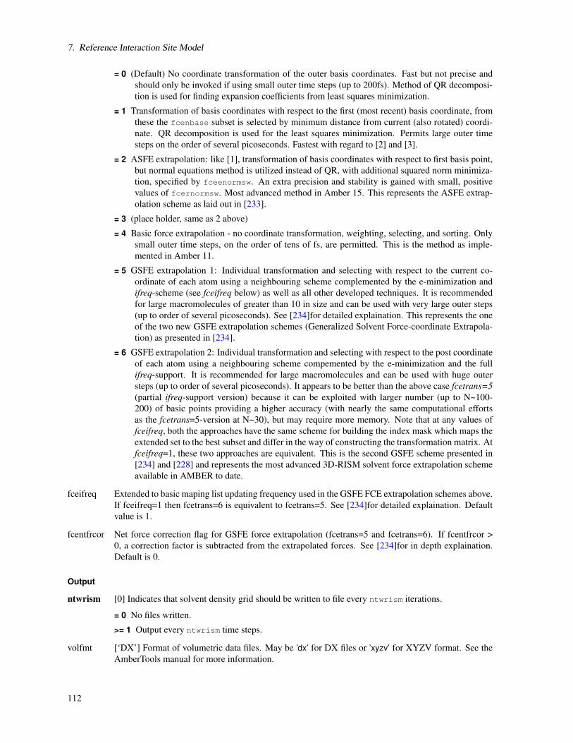
7. Reference Interaction Site Model
= 0 (Default) No coordinate transformation of the outer basis coordinates. Fast but not precise andshould only be invoked if using small outer time steps (up to 200fs). Method of QR decomposi-tion is used for finding expansion coefficients from least squares minimization.
= 1 Transformation of basis coordinates with respect to the first (most recent) basis coordinate, fromthese the fcenbase subset is selected by minimum distance from current (also rotated) coordi-nate. QR decomposition is used for the least squares minimization. Permits large outer timesteps on the order of several picoseconds. Fastest with regard to [2] and [3].
= 2 ASFE extrapolation: like [1], transformation of basis coordinates with respect to first basis point,but normal equations method is utilized instead of QR, with additional squared norm minimiza-tion, specified by fceenormsw. An extra precision and stability is gained with small, positivevalues of fcernormsw. Most advanced method in Amber 15. This represents the ASFE extrap-olation scheme as laid out in [233].
= 3 (place holder, same as 2 above)
= 4 Basic force extrapolation - no coordinate transformation, weighting, selecting, and sorting. Onlysmall outer time steps, on the order of tens of fs, are permitted. This is the method as imple-mented in Amber 11.
= 5 GSFE extrapolation 1: Individual transformation and selecting with respect to the current co-ordinate of each atom using a neighbouring scheme complemented by the e-minimization andifreq-scheme (see fceifreq below) as well as all other developed techniques. It is recommendedfor large macromolecules of greater than 10 in size and can be used with very large outer steps(up to order of several picoseconds). See [234]for detailed explaination. This represents the oneof the two new GSFE extrapolation schemes (Generalized Solvent Force-coordinate Extrapola-tion) as presented in [234].
= 6 GSFE extrapolation 2: Individual transformation and selecting with respect to the post coordinateof each atom using a neighbouring scheme compemented by the e-minimization and the fullifreq-support. It is recommended for large macromolecules and can be used with huge outersteps (up to order of several picoseconds). It appears to be better than the above case fcetrans=5(partial ifreq-support version) because it can be exploited with larger number (up to N~100-200) of basic points providing a higher accuracy (with nearly the same computational effortsas the fcetrans=5-version at N~30), but may require more memory. Note that at any values offceifreq, both the approaches have the same scheme for building the index mask which maps theextended set to the best subset and differ in the way of constructing the transformation matrix. Atfceifreq=1, these two approaches are equivalent. This is the second GSFE scheme presented in[234] and [228] and represents the most advanced 3D-RISM solvent force extrapolation schemeavailable in AMBER to date.
fceifreq Extended to basic maping list updating frequency used in the GSFE FCE extrapolation schemes above.If fceifreq=1 then fcetrans=6 is equivalent to fcetrans=5. See [234]for detailed explaination. Defaultvalue is 1.
fcentfrcor Net force correction flag for GSFE force extrapolation (fcetrans=5 and fcetrans=6). If fcentfrcor >0, a correction factor is subtracted from the extrapolated forces. See [234]for in depth explaination.Default is 0.
Output
ntwrism [0] Indicates that solvent density grid should be written to file every ntwrism iterations.
= 0 No files written.
>= 1 Output every ntwrism time steps.
volfmt [‘DX’] Format of volumetric data files. May be ’dx’ for DX files or ’xyzv’ for XYZV format. See theAmberTools manual for more information.
112

7.7. 3D-RISM in sander
verbose [0] Indicates level of diagnostic detail about the calculation written to the log file.
= 0 No output.
= 1 Print the number of iterations used to converge.
= 2 Print details for each iteration and information about what FCE is doing every progress itera-tions.
write_thermo [1] Print solvation thermodynamics in addition to standard sander output. The format is the sameas that found in NAB and rism3d.snglpnt.
polarDecomp [0] Decomposes solvation free energy into polar and non-polar components. Note that this typicallyrequires 80% more computation time.
= 0 No polar/non-polar decomposition.
= 1 Polar/non-polar decomposition.
entropicDecomp [0] Decomposes solvation free energy into energy and entropy components. Also performstemperature derivatives of other calculated quantities. Note that this typically requires 80% morecomputation time and requires a .xvv file version 1.000 or higher (see §7.1.3 and 7.3).
= 0 No entropic decomposition.
= 1 Entropic decomposition.
progress [1] Display progress of the 3D-RISM solution every kshow iterations. 0 indicates this information willnot be displayed. Must be used with verbose> 1.
7.7.2.2. Example
Molecular Dynamics (imin=0)
molecular dynamics with 3D-RISM and impulse MTS
&cntrl
ntx=1, ntpr=100, ntwx=1000,ntwr=10000,
nstlim=10000,dt=0.001, !No shake or r-RESPA
ntt=3, temp0=300, gamma_ln=20, !Langevin dynamics
ntb=0, !Non-periodic
cut=999., !Calculate all
!solute-solute
!interactions
irism=1,
/
&rism
rismnrespa=5, !r-RESPA MTS
fcenbasis=10,fcestride=2,fcecrd=2 !FCE MTS
/
Minimization (imin=1)
Default XMIN minimization with 3D-RISM
&cntrl
imin=1, maxcyc=200,
drms=1e-3, !RMS force. Can be as low as 1e-4
ntmin=3, !XMIN
ntpr=5,
ntb=0, !Non-periodic
113

7. Reference Interaction Site Model
cut=999., !Calculate all
!solute-solute interactions
irism=1
/
&rism
tolerance=1e-11, !Low tolerance
solvcut=9999, !No cut-off for
!solute-solvent interactions
centering=2 !Solvation box centering
!using center-of-geometry
/
Trajectory Post-Processing (imin=5)
Trajectory post-processing with 3D-RISM
&cntrl
ntx=1, ntpr=1, ntwx=1,
imin=5,maxcyc=1, !Single-point energy calculation
!on each frame
ntb=0, !Non-periodic
cut=9999., !Calculate all
!solute-solute interactions
irism=1
/
&rism
tolerance=1e-4, !Saves some time compared to 1e-5
apply_rism_force=0, !Saves some time. Forces are not used.
npropagate=1 !Saves some time and 4*8*Nbox bytes
!of memory compared to npropagate=5.
/
7.8. RISM File Formats
7.8.1. MDL
Solvent MoDeL (MDL) files use the prmtop specification. Each of the following sections may appear in the filein any order. The Fortran string format specifications can be different from the recommend values below.
%VERSION VERSION_STAMP = Vxxxx.yyy DATE = mm:dd:yy hh:mm:ss
The current version of the format is 0001.000. Date should be the date and time the file is created.
%FLAG TITLE
%FORMAT(20a4)
Optional description of the file.
%FLAG POINTERS
%FORMAT(10I8)
Defines the lengths of arrays in the file.
NATOM Number of physical atoms in the model.
NSITE Number of unique solvent sites (share common Lennard-Jones parameters and partial charges).
114

7.8. RISM File Formats
%FLAG ATMNAME
%FORMAT(20a4)
CHARACTER(len=4)(NSITE) Four character name of each solvent site.
%FLAG MASS
%FORMAT(5e16.8)
REAL*8(NSITE) Mass of each solvent site (amu).
%FLAG CHG
%FORMAT(5e16.8)
REAL*8(NSITE) Partial charge for each solvent site, 18.2223e (√
kT Å).
%FLAG LJEPSILON
%FORMAT(5e16.8)
REAL*8(NSITE) Lennard-Jones ε for each solvent site (kcal/mol).
%FLAG LJSIGMA
%FORMAT(5e16.8)
REAL*8(NSITE) Lennard-Jones rmin/2 (sometimes called σ∗/2) for each solvent site (Å)
ULJαγ =
√εα εγ
((rmin,α + rmin,γ
2r
)12
−2(
rmin,α + rmin,γ
2r
)6).
Note that this is related to the commonly used σ as
σ = rmin2−1/6.
%FLAG MULTI
%FORMAT(10I8)
INTEGER*4(NSITE) Multiplicity of each solvent site. This should sum to NATOM.
%FLAG COORD
%FORMAT(5e16.8)
REAL*8(3*NATOM) xyz-coordinates of each atom (Å).
7.8.2. XVV
The .xvv file provides all of the bulk-solvent information required for 3D-RISM. This includes informationabout the solvent model, thermodynamic state and the necessary correlation functions. .xvv files use the prmtopspecification. Each of the following sections may appear in the file in any order. The format specifications can bedifferent from the recommend values below.
1D- and 3D-RISM now use version 1.000 of the file format. Differences include
• additional information about solvent, such as mass, number of sites per species, coordinates;
• RISM’s internal system of units is now used;
• temperature derivative, DELHV0_DT and XVV_DT, are included when available (see 7.4.1);
• and SIGV has been replaced by RMIN2V.
115
7. Reference Interaction Site Model
All 3D-RISM interfaces still support the original 0.001 version of the format. For detailed information on version0.001, please see the AmberTools 1.5 manual.
%VERSION VERSION_STAMP = V0001.000 DATE = mm:dd:yy hh:mm:ss
The current version of the format is 0001.000. Date should be the date and time the file is created.
%FLAG POINTERS
%FORMAT(10I8)
Defines the lengths of arrays in the file.
NR Number of 1D grid points in χVVab (k).
NV Number of total solvent sites.
NSP Number of solvent species (molecules).
%FLAG THERMO
%FORMAT(1PE24.16)
REAL(8)(6) Temperature [K], dielectric constant, inverse Debye length (κ) [Å], compressibility [Å−3], grid spac-ing [Å], charge smear [Å].
%FLAG ATOM_NAME
%FORMAT(20A4)
CHARACTER(len=4)(NSITE) Four character name of each solvent site.
%FLAG MTV
%FORMAT(10I8)
INTEGER(4)(NSITE) Multiplicity of each solvent site.
%FLAG NVSP
%FORMAT(10I8)
INTEGER(4)(NSP) Number of sites for each solvent species.
%FLAG MASS
%FORMAT(1P5E16.8)
REAL(8)(NSITE) Mass of each solvent site (g/mol).
%FLAG RHOV
%FORMAT(1P5E16.8)
REAL(8)(NSITE) Number density of each solvent site (Å−3).
%FLAG QV
%FORMAT(1P5E16.8)
REAL(8)(NSITE) Partial charge for each solvent site multiplied by the square root of the Coulomb constant,~18.2223 (
√kT Å).
%FLAG QSPV
%FORMAT(1P5E16.8)
116
7.8. RISM File Formats
REAL(8)(NSPECIES) Net charge for each solvent species multiplied by the square root of the Coulomb constant,~18.2223 (
√kT Å).
%FLAG EPSV
%FORMAT(1P5E16.8)
REAL(8)(NSITE) Lennard-Jones ε for each solvent site (kT ).
%FLAG RMIN2V
%FORMAT(1P5E16.8)
REAL(8)(NSITE) Lennard-Jones rmin/2 (σ∗/2) for each solvent site (Å).
%FLAG DELHV0
%FORMAT(1P5E16.8)
REAL(8)(NSITE) Long range Coulomb correction for each solvent site (√
kT Å).
%FLAG DELHV0_DT
%FORMAT(1P5E16.8)
REAL(8)(NSITE) (Optional) Temperature derivative long range Coulomb correction for each solvent site (√
kT Å).
%FLAG COORD
%FORMAT(1P5E16.8)
REAL(8)(3*sum(MTV)) Coordinates of all atoms (not sites) for each solvent species with the dipole momentaligned with the z-axis (Å).
%FLAG XVV
%FORMAT(1P5E16.8)
REAL(8)(NR,NSITE,NSITE) χVVab (k). This array is stored in column major order. That is, the NR index varies
fastest.
%FLAG XVV_DT
%FORMAT(1P5E16.8)
REAL(8)(NR,NSITE,NSITE) (Optional) δT χVVab (k). This array is stored in column major order. That is, the NR
index varies fastest.
7.8.3. Site-site functionals
All .*vv files, except .xvv (see §7.8.2), provide the separation dependence of all site-site pairings for a particularfunctional and use the same format. The first four lines have a “#” in the first character column, provide a descrip-tion of the contents of the file and indicate site-site pairs. The first data column is the site-site separation and theremaining columns provide the value of the functional for the site-site pair at this separation.
The following example is for the direct correlation function (.cvv) for pure water. A standard, ‘two-site’ watermodel is used, consisting of oxygen (O) and hydrogen (H1). This gives one solvent species with two atoms.
#RISM1D ATOM-ATOM INTERACTIONS: DIRECT CORRELATION VS. SEPARATION [A]
#S=SPECIES, A=ATOM
# SEPARATION S1A1:S1A1 S1A1:S1A2 S1A2:S1A2
# SEPARATION O:O H1:O H1:H1
0.00000000E+000 -3.81875841E+002 1.64156197E+002 -9.24562553E+001
2.50000000E-002 -3.81695327E+002 1.64139031E+002 -9.24384608E+001
117

7. Reference Interaction Site Model
7.8.4. Thermodynamics
Thermodynamic output is divided into global, species and site properties sections. Global properties are gen-erally not decomposable into species or site contributions (e.g., pressure). Species properties are the values forindividual molecular species, for example, the excess chemical potential of a single molecule. Some of theseproperties, such as the partial molar volume, may not be decomposible into individual sites. Site properties arecontributions from individual sites. Values for sites from the same species will sum to give the total value for thespecies.
The file format is white-space delimited with the first three columns giving a description, variable name andunits of the property calculated. The remaining columns contain the calculated values for the system, species orsite. Descriptive lines are indicated with a leading “#”.
The following example is for a standard, ‘two-site’ water model is used, consisting of oxygen (O) andhydrogen (H1), at standard temperature and density. In this calculation, energy/entropy free energydecomposition is also performed. I.e., EXCHEMsp= ESOLVsp−TSsp.
#Global properties
#Description Variable Units Value
Compressibility xi [10e-4/MPa] 4.73552130E+000
Pressure_(Virial) Pvir [MPa] 2.51627507E+003
Excess_free_energy FE [kcal/mol] -1.03698038E+003
#Species properties
#Description Variable Units SPC
Excess_chemical_potential EXCHEMsp [kcal/mol] -2.79190339E+000
Solvation_energy ESOLVsp [kcal/mol] -1.16421825E+001
-Temperature*solvation_entropy -TSsp [kcal/mol] 8.85027911E+000
Partial_molar_volume PMV [A^-3] 3.00300236E+001
#Site properties
#Description Variable Units O H1
Excess_chemical_potential EXCHEMv [kcal/mol] -6.47897321E+000 3.68706981E+000
Solvation_energy ESOLVv [kcal/mol] -1.19565867E+001 3.14404192E-001
-Temperature*solvation_entropy -TSv [kcal/mol] 5.47761350E+000 3.37266562E+000
7.8.5. Total excess values
.n00 and .q00 files provide the total excess coordination number and charge about each solvent site. The totalexcess of site γ around site α is
nextotαγ = ργ
∫∞
0hαγ (r)dr,
while the total excess charge isqextot
αγ = qγ nextotαγ .
These values are presented in their respective files as nsite×nsite arrays. Any asymmetry in these arrays is due tonumerical error. .q00 files additionally provided the total excess charge from all sites.
The following example gives the total excess charge for a standard, ‘two-site’ water model is used, consistingof oxygen (O) and hydrogen (H1), at standard temperature and density.
#Total excess coordinated charge [e] of column site about row site
O H1 Total charge
O 7.92607232E-001 -7.92607230E-001 1.67181313E-009
H1 7.92607231E-001 -7.92607229E-001 2.44386922E-009
7.8.6. DX volumetric data
By default, 3D correlation functions from 3D-RISM calculations use the ASCII version of the Data Explorer(DX) file format for volumetric data on regular grids as defined in the DX user manual: http://opendx.
informatics.jax.org/docs/html/pages/usrgu068.htm#HDREDF.
118

7.8. RISM File Formats
Header
object 1 class gridpositions counts Nx Ny Nz
Nx INTEGER*4. Number of grid points in the x dimension.
Ny INTEGER*4. Number of grid points in the y dimension.
Nz INTEGER*4. Number of grid points in the z dimension.
origin Ox Oy Oz
Ox REAL*8. x coordinate of grid origin in Cartesian space.
Oy REAL*8. y coordinate of grid origin in Cartesian space.
Oz REAL*8. z coordinate of grid origin in Cartesian space.
delta dx 0 0
delta 0 dy 0
delta 0 0 dz
dx REAL*8. Linear grid size between in the x dimension.
dy REAL*8. Linear grid size between in the y dimension.
dz REAL*8. Linear grid size between in the z dimension.
object 2 class gridconnections counts Nx Ny Nz
object 3 class array type double rank 0 items N data follows
N INTEGER*4. N= Nx×Ny×Nz.
Data
data(i,j,k) data(i,j,k+1) data(i,j,k+2)
data(i,j,k) REAL*8. Three data values per line with the last (z) index varying fastest for a total of N values.
Footer
object "Untitled" call field
7.8.7. XYZV volumetric data
An alternate format for volumetric data is the simple ASCII x-y-z-value (XYZV) format. The x-, y- andz-coordinates each grid point is written on a line followed by the value of the grid point. There is no header orfooter. For example,
...
-7.10789855E+000 -1.12570084E+001 -1.61284113E+001 1.35771922E-006
-2.10789855E+000 -1.12570084E+001 -1.61284113E+001 -5.32279347E-006
2.89210145E+000 -1.12570084E+001 -1.61284113E+001 -1.58802759E-005
119
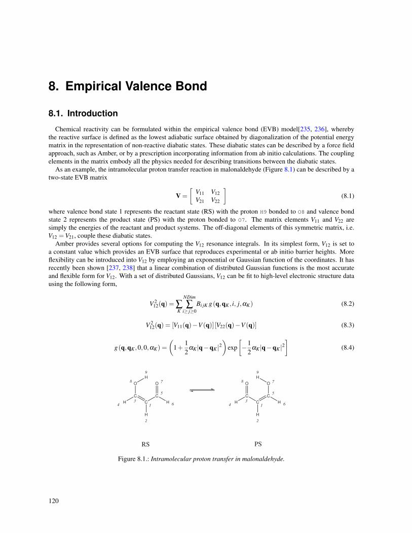
8. Empirical Valence Bond
8.1. Introduction
Chemical reactivity can be formulated within the empirical valence bond (EVB) model[235, 236], wherebythe reactive surface is defined as the lowest adiabatic surface obtained by diagonalization of the potential energymatrix in the representation of non-reactive diabatic states. These diabatic states can be described by a force fieldapproach, such as Amber, or by a prescription incorporating information from ab initio calculations. The couplingelements in the matrix embody all the physics needed for describing transitions between the diabatic states.
As an example, the intramolecular proton transfer reaction in malonaldehyde (Figure 8.1) can be described by atwo-state EVB matrix
V =
[V11 V12V21 V22
](8.1)
where valence bond state 1 represents the reactant state (RS) with the proton H9 bonded to O8 and valence bondstate 2 represents the product state (PS) with the proton bonded to O7. The matrix elements V11 and V22 aresimply the energies of the reactant and product systems. The off-diagonal elements of this symmetric matrix, i.e.V12 =V21, couple these diabatic states.
Amber provides several options for computing the V12 resonance integrals. In its simplest form, V12 is set toa constant value which provides an EVB surface that reproduces experimental or ab initio barrier heights. Moreflexibility can be introduced into V12 by employing an exponential or Gaussian function of the coordinates. It hasrecently been shown [237, 238] that a linear combination of distributed Gaussian functions is the most accurateand flexible form for V12. With a set of distributed Gaussians, V12 can be fit to high-level electronic structure datausing the following form,
V 212(q) = ∑
K
NDim
∑i≥ j≥0
Bi jK g(q,qK , i, j,αK) (8.2)
V 212(q) = [V11(q)−V (q)] [V22(q)−V (q)] (8.3)
g(q,qK ,0,0,αK) =
(1+
12
αK |q−qK |2)
exp[−1
2αK |q−qK |2
](8.4)
C
C
C
OO
H
H
9
7
5
1
3
8
4
2
6
RS PS
H
H
C
C
C
OO
H
H
9
7
5
1
3
8
4
2
6
H
H
Figure 8.1.: Intramolecular proton transfer in malonaldehyde.
120

8.2. General usage description
g(q,qK , i,0,αK) = (q−qK)i exp[−1
2αK |q−qK |2
](8.5)
g(q,qK , i, j,αK) = (q−qK)i (q−qK) j exp[−1
2αK |q−qK |2
](8.6)
where g(q,qK , i, j,αK) are s-, p-, and d-type Gaussians at a number of points, qK , on the potential energy surface,NDim is the total number of internal coordinates, V is the ab initio energy and B is a vector of coefficients. Itis important to note that a nonstandard s-type Gaussian is employed to precondition the resulting set of linearequations that is passed to a GMRES[239] (aka DIIS[240, 241]) solver. For a more exhaustive discussion of theDG EVB method please see reference [238]. Additionally, the EVB facility in Amber can perform MD or energyoptimization on the EVB ground-state surface and biased sampling along a predefined reaction coordinate (RC).Nuclear quantization based on the Feynman path integral formalism [242–244] is also possible.
8.2. General usage description
The EVB facility is built on top of the multisander infrastructure in Amber. (Section 18.11) As such, the userwill need to build the parallel version of sander in order to utilize the EVB feature. Information for each EVBdiabatic state is obtained from separate (simultaneous) instances of sander. The energies and forces of all the statesare communicated via MPI to the master node, which is responsible for computing the EVB energy and forces andbroadcasting these to the other nodes for the next MD step.
The required input files are (1) an EVB multisander group file containing per line all the command line optionsfor each sander job, (2) the mdin, coordinate, and parmtop files specified in the group file, and (3) the EVB inputfiles. At the top level, an EVB calculation is invoked as follows:
mpirun -np <# procs> sander.MPI -ng <# groups> -groupfile <EVB group file>
The contents of the EVB group file is similar to that for a conventional multisander execution, with the additionof a command line flag -evbin for specifying the name of the EVB input file. Below is an example of an EVBgroup file:
# Malonaldehyde RS: H9 bonded to O8
-O -i mdin -p mr.top -c mr.crd -o mr.out -r mr.rst -evbin input.mr
# Malonaldehyde PS: H9 bonded to O7
-O -i mdin -p mp.top -c mr.crd -o mp.out -r mp.rst -evbin input.mp
Each line corresponds to a diabatic state, and comments are preceded by a # symbol in the first column of a line.Now, it is important to notice in the above example that the starting configurations for both sander jobs are thesame, although the topology files are different. This constraint guarantees that the system starts in a physicallymeaningful part of configuration space. Furthermore, it is critical that the atom numbers (delineating the atomlocations in the coordinate and parmtop files) are identical among the EVB diabatic states. In Figure 8.1, forexample, the atom numbers of the RS and PS malonaldehydes are identical. The only additional flag in the &cntrlnamelist of the mdin file is ievb, which has the following values
ievb Flag to run EVB
= 0 No effect (default)
= 1 Enable EVB. The value of imin specifies if the sander calculation is a molecular dynam-ics (imin=0) or an energy minimization (imin=1). The variable evb_dyn in the &evbnamelist of the EVB input file refines this choice to specify if the calculation type is onthe EVB ground-state surface, on a mapping potential, or on a biased potential.
The argument of the command line flag -evbin provides the name of the EVB input file. Corresponding to theabove group file example, the inputs for EVB state 1 are provided in the file input.mr and those for EVB state 2are provided in input.mp. For the case of constant coupling between the EVB states, the file input.mr may looklike the following:
121

8. Empirical Valence Bond
# Malonaldehyde RS: proton (H9) bound to O8
&evb nevb = 2, nbias = 1, nmorse = 1, nmodvdw = 1, ntw_evb = 50,
xch_type = "constant",
evb_dyn = "egap_umb",
dia_shift(1)%st = 1, dia_shift(1)%nrg_offset = 0.0,
dia_shift(2)%st = 2, dia_shift(2)%nrg_offset = 0.0,
xch_cnst(1)%ist = 1, xch_cnst(1)%jst = 2,
xch_cnst(1)%xcnst = 12.5,
egap_umb(1)%ist = 1, egap_umb(1)%jst = 2,
egap_umb(1)%k = 0.005, egap_umb(1)%ezero = 0.0,
morsify(1)%iatom = 8, morsify(1)%jatom = 9, morsify(1)%D = 356.570,
morsify(1)%a = 1.046, morsify(1)%r0 = 1.000,
modvdw(1)%iatom = 9, modvdw(1)%jatom = 7,
/
and the file input.mp may appear as follows:
# Malonaldehyde PS: proton (H9) bound to O7
&evb nevb = 2, nbias = 1, nmorse = 1, nmodvdw = 1, ntw_evb = 50,
xch_type = "constant",
evb_dyn = "egap_umb",
dia_shift(1)%st = 1, dia_shift(1)%nrg_offset = 0.0,
dia_shift(2)%st = 2, dia_shift(2)%nrg_offset = 0.0,
xch_cnst(1)%ist = 1, xch_cnst(1)%jst = 2,
xch_cnst(1)%xcnst = 12.5,
egap_umb(1)%ist = 1, egap_umb(1)%jst = 2,
egap_umb(1)%k = 0.005, egap_umb(1)%ezero = 0.0,
morsify(1)%iatom = 7, morsify(1)%jatom = 9, morsify(1)%D = 356.570,
morsify(1)%a = 1.046, morsify(1)%r0 = 1.000,
modvdw(1)%iatom = 9, modvdw(1)%jatom = 8,
/
The above EVB files specify that the system is described by a two-state model, the coupling between the two-statesis a constant, and the dynamics is umbrella sampling along an energy gap RC. Since the reactant and product statesare identical by symmetry, no adjustments of the relative energies of the diabatic states are performed. The constantvalue coupling between the two states is parameterized such that the EVB barrier reproduces the ab initio barrier of~ 3 kcal/mol (RMP2/cc-pVTZ level). Lastly, the standard Amber harmonic bond interactions involving the protonwith the donor and acceptor oxygens are replaced by Morse functions and certain van der Waals interactions areexcluded.
This parameterization of the EVB surface to provide observables that match either results from high-level quan-tum chemistry calculations or experimental measurements is the trickiest aspect of the EVB model. However, afterthe EVB surface has been calibrated, the user has access to reactive chemical dynamics simulation timescales andlengthscales which would be otherwise inaccessible using conventional ab initio MD approaches. The distributedGaussian EVB framework provides a systematic procedure for computing V12 from ab initio data.
Now, let us suppose that the constant coupling prescription does not provide the detailed features needed todescribe the reaction pathway. Furthermore, we find that the coupling as a function of the coordinates can bedescribed adequately (from comparison to ab initio data) using a Gaussian functional form. How should onemodify the above EVB input files to obtain a more accurate reactive surface? We need to change the xch_typevariable from “constant” to “gauss” as well as replace the variable xch_cnst by the variable xch_gauss(:), whichcontains the parameters for the Gaussian functional form. Of course, these parameters need to be optimized toprovide the more accurate surface. The modifications to the EVB input files look something like the following,
...
xch_type = "constant",
122

8.3. Biased sampling
xch_type = "gauss",...
xch_cnst(1)%ist = 1, xch_cnst(1)%jst = 2,
xch_cnst(1)%xcnst = 12.5,
xch_gauss(1)%ist = 1, xch_gauss(1)%jst = 2,
xch_gauss(1)%iatom = 8, xch_gauss(1)%jatom = 7,
xch_gauss(1)%a = 11.0, xch_gauss(1)%sigma = 0.0447,
xch_gauss(1)%r0 = 2.3,...
where the cross-through lines have been replaced by those below them. Access to the exponential functional formor the distributed Gaussian approximation to V12 entails similar changes to the input files. Please see $AMBER-HOME/test/evb for examples.
8.3. Biased sampling
When a reactive event is described by an intrinsic high free energy barrier, molecular dynamics on the EVBground-state surface will not adequately sample the important transition state region. Under these conditions,chemical reactions are rare events and sampling on the EVB surface effectively reduces to sampling on a diabaticsurface. One framework for enhancing the sampling of rare events is through modification of the system Hamilto-nian with the addition of biasing potentials. The EVB facility in Amber offers several options for biased sampling:(1) Ariel Warshel’s mapping potential approach[235] (2) Dave Case’s umbrella sampling on an energy gap RC (3)umbrella sampling on a distance RC and (4) umbrella sampling on a difference of distances RC.
In the mapping potential framework, the system Hamiltonian (and hence, the molecular dynamics) is describedby the modified potential
Vλ = (1−λ )Vii +λVf f (8.7)
where Vii is the EVB matrix element for the initial state and Vf f is the EVB matrix element for the final state. Asthe value of the mapping potential parameter λ changes from 0 to 1, the system evolves from the initial state to thefinal state. As an example, for λ = 0.50, the system Hamiltonian is an equal linear combination of the initial andfinal states and molecular dynamics sample the region in the vicinity of the transition state. Each mapping potentialVλ samples only a portion of the reaction coordinate. In practice, a series of mapping potentials are used to biasthe sampling across the entire range of the RC. The average distribution of the RC for each mapping potential isthen unbiased and the set of unbiased distributions are combined to give the potential of mean force (PMF) on theEVB ground-state surface. Figure 8.2 shows a PMF for the malonaldehyde intramolecular proton transfer reactionas obtained from 9 mapping potential simulations with λ ranging from 0.10 to 0.90 at 0.10 intervals.
In the umbrella sampling framework, the system Hamiltonian is described by the modified potential
V (n)biased(q) = Vel0(q)+V (n)
umb(q)
= Vel0(q)+12
k(n)[RC(q)−RC(n)
0
]2(8.8)
where q is the set of system coordinates, k is the harmonic force constant parameter, and V (n)umb is an umbrella
potential that is added to the original system potential Vel0 (obtained from diagonalization of the EVB matrix) tobias the sampling towards a particular value of the reaction coordinate RC(n)
0 . The superscript (n) denotes that aseries of biased simulations, each enhancing the sampling of a particular window of the RC, is required to map outthe entire PMF. The number of umbrella sampling windows as well as the choice of values for the force constantparameter and the RC equilibrium position will depend ultimately on the nature of the free energy landscape of thesystem in question.
123

8. Empirical Valence Bond
-75 -50 -25 0 25 50 75
Collective Reaction Coordinate [kcal/mol]
0
1
2
3
Pote
nti
al
of
Mean F
orc
e [
kcal/
mol]
Figure 8.2.: Potential of mean force along an energy gap RC for the intramolecular proton transfer in malonalde-hyde as obtained from a series of mapping potential simulations.
evb_dyn dependency“evb_map” ⇒ emap(:)
“egap_umb” ⇒ egap_umb(:)“bond_umb” ⇒ bond_umb(:)
“dbonds_umb” ⇒ dbonds_umb(:)“qi_bond_pmf” ⇒ bond_umb(:)“qi_bond_dyn” ⇒ bond_umb(:)
“qi_dbonds_pmf” ⇒ dbonds_umb(:)“qi_dbonds_dyn” ⇒ dbonds_umb(:)
Table 8.2.: Derived variable types for EVB.
Results from the biased samplings then can be unbiased and combined using the weighted histogram analysismethod (WHAM)[245–247] to generate the PMF describing chemistry on the physically relevant EVB ground-state potential energy surface, Vel0. Figure 8.3 depicts the PMF for the malonaldehyde intramolecular protontransfer that is obtained from 13 umbrella sampling simulations with RC(n)
0 spanning the range -60 kcal/mol to +60kcal/mol at 10 kcal/mol intervals. The supporting program to generate the PMF from a set of mapping potential orfrom a set of umbrella sampling simulations can be obtained from the Amber website, http://ambermd.org.
Biased sampling is accessed through the nbias and evb_dyn variables in the EVB input file. The variable nbiasspecifies the number of biasing potentials to include in the system Hamiltonian. Mapping potential dynamics isinvoked using the assignment evb_dyn=“evb_map”. Biased sampling via umbrella potentials is invoked with theassignment evb_dyn=“egap_umb”, evb_dyn=“bond_umb” or evb_dyn=“dbonds_umb”. Associated with eachchoice of biased sampling approach is a derived type variable that provides the required parameters, as shown inTable 8.2. Please see Section 8.6 for more details about the variable dependencies.
124

8.3. Biased sampling
-75 -50 -25 0 25 50 75
Collective Reaction Coordinate [kcal/mol]
0
1
2
3
Pote
nti
al
of
Mean F
orc
e [
kcal/
mol]
Figure 8.3.: Potential of mean force for the intramolecular proton transfer in malonaldehyde as obtained from aseries of umbrella sampling simulations along an energy gap RC. The distributions of the RC from allthe windows are combined using the WHAM procedure.
125

8. Empirical Valence Bond
8.4. Quantization of nuclear degrees of freedom
The EVB framework provides a computationally practical approximation to the electronic surface for modelingchemical reactions involving classical atoms. The full Schrödinger equation, nevertheless, describes not only theelectrons but also the nuclei as a wave function. This quantum mechanical description of nuclei is particularlyimportant for capturing the nuclear dispersion of light particles, such as hydrogen. We provide quantization of thenuclear degrees of freedom via coupling of the EVB facility with the Feynman Path-Integral Molecular Dynamicsfunction in Amber [242–244]. The current implementation utilizes the PIMD engine that is built on top of thelocally enhanced sampling (LES) infrastructure. As such, the user will need to build the parallel version of LESsander in order to utilize EVB/LES-PIMD.
PIMD is invoked using the ipimd variable (and associated dependencies) in the &cntrl namelist of the mdininput file (please consult Section 26.1.2). The requirements for EVB within the EVB/LES-PIMD context aresimilar to those described for classical EVB but with the coordinate and parmtop files modified for a LES-typecalculation, where the number of LES copies correspond to the number of path integral slices. For example, aclassical EVB umbrella sampling on a difference of distances RC will have EVB input files similar to the aboveexamples but with the following modifications
...
evb_dyn = "dbonds_umb",...
dbonds_umb(1)%iatom = 8, dbonds_umb(1)%jatom = 9, dbonds_umb(1)%katom = 7,
dbonds_umb(1)%k = 100.000, dbonds_umb(1)%ezero = -.20,...
EVB/LES-PIMD utilizes these same EVB input files. The EVB group file evb.grpfile, however, has been modifiedto point to the LES coordinate and parmtop files
# 32-bead Malonaldehyde RS: H9 bonded to O8
-O -i mdin -p mr_les.top -c mr_les.crd -o mr_les.out -r mr_les.rst \
-evbin input.mr
# 32-bead Malonaldehyde PS: H9 bonded to O7
-O -i mdin -p mp_les.top -c mr_les.crd -o mp_les.out -r mp_les.rst \
-evbin input.mp
Additionally, the -nslice <# PIMD slices> variable must be passed to the sander executable:
mpirun -np 2 sander.LES.MPI -ng 2 -nslice 32 -groupfile evb.grpfile
Here, the atoms of the malonaldehyde system have been replicated into 32 copies using the addles utility (seeSection 26.1.2) and each of the EVB diabatic states now use the corresponding LES coordinate and parmtop files.Nuclear quantization lowers the free energy barrier due to quantum mechanical effects, such as zero point motionand tunneling. Figure 8.4 compares the PMFs for the malonaldehyde proton transfer reaction along a differenceof distances RC from classical EVB and EVB/PIMD umbrella sampling simulations. Currently, only the distanceand difference of distances RCs are supported in EVB/PIMD. The energy gap RC is not supported because thetheoretical formulation of quantum transition state theory based on an energy gap RC has not yet been worked out.
8.5. Distributed Gaussian EVB
As briefly mentioned in the Introduction to EVB, V12 can be fit to high-level electronic structure data using aset of s-, p-, and d-type Gaussians as the fitting basis functions. The current incarnation of DG EVB is limited totwo-state gas-phase systems. Current efforts to extend this approach to the condensed phase will provide apractical systematic procedure for constructing a reactive surface from ab initio information. The curious studentis encouraged to read the original papers on this method for the theoretical formulation[237, 238]. Here, we only
126
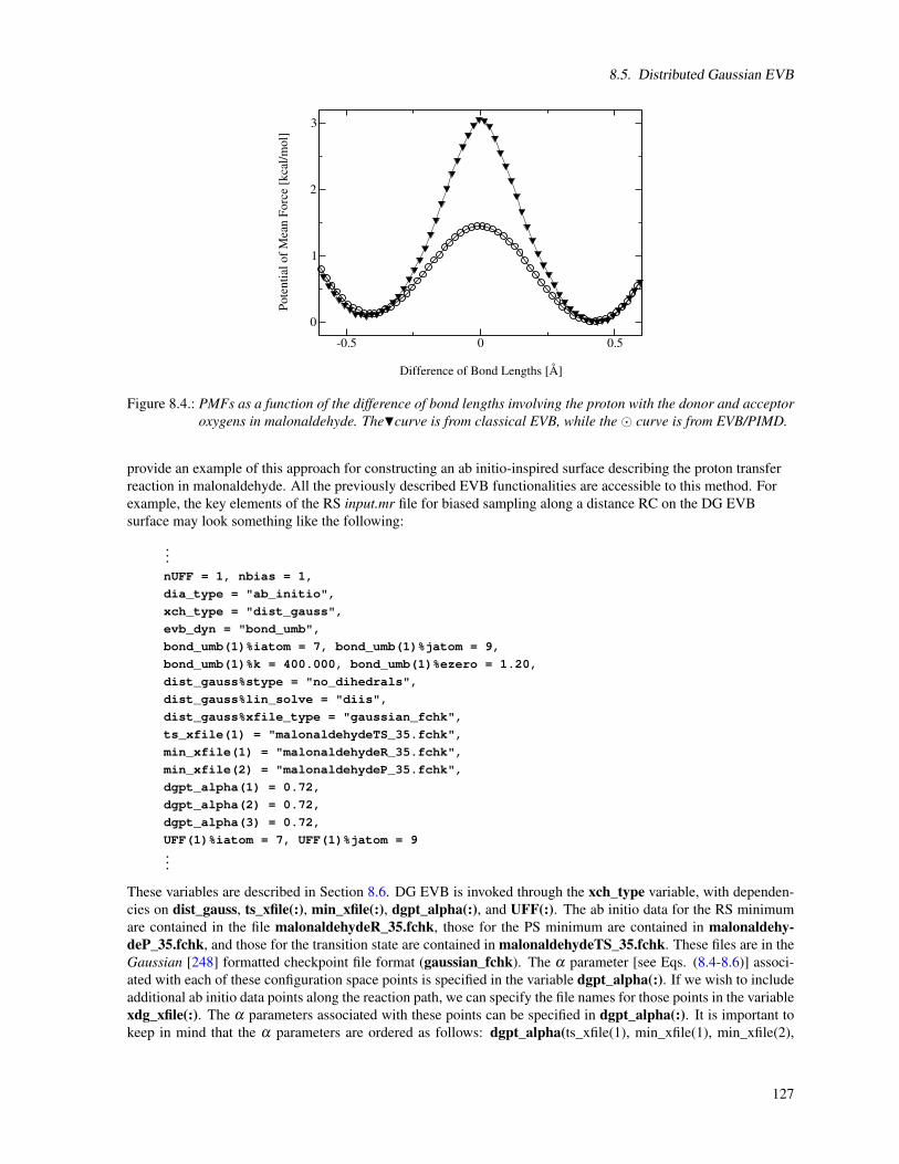
8.5. Distributed Gaussian EVB
-0.5 0 0.5
Difference of Bond Lengths [Å]
0
1
2
3
Pote
ntia
l of
Mea
n Fo
rce
[kca
l/mol
]
Figure 8.4.: PMFs as a function of the difference of bond lengths involving the proton with the donor and acceptoroxygens in malonaldehyde. TheHcurve is from classical EVB, while the curve is from EVB/PIMD.
provide an example of this approach for constructing an ab initio-inspired surface describing the proton transferreaction in malonaldehyde. All the previously described EVB functionalities are accessible to this method. Forexample, the key elements of the RS input.mr file for biased sampling along a distance RC on the DG EVBsurface may look something like the following:
...
nUFF = 1, nbias = 1,
dia_type = "ab_initio",
xch_type = "dist_gauss",
evb_dyn = "bond_umb",
bond_umb(1)%iatom = 7, bond_umb(1)%jatom = 9,
bond_umb(1)%k = 400.000, bond_umb(1)%ezero = 1.20,
dist_gauss%stype = "no_dihedrals",
dist_gauss%lin_solve = "diis",
dist_gauss%xfile_type = "gaussian_fchk",
ts_xfile(1) = "malonaldehydeTS_35.fchk",
min_xfile(1) = "malonaldehydeR_35.fchk",
min_xfile(2) = "malonaldehydeP_35.fchk",
dgpt_alpha(1) = 0.72,
dgpt_alpha(2) = 0.72,
dgpt_alpha(3) = 0.72,
UFF(1)%iatom = 7, UFF(1)%jatom = 9...
These variables are described in Section 8.6. DG EVB is invoked through the xch_type variable, with dependen-cies on dist_gauss, ts_xfile(:), min_xfile(:), dgpt_alpha(:), and UFF(:). The ab initio data for the RS minimumare contained in the file malonaldehydeR_35.fchk, those for the PS minimum are contained in malonaldehy-deP_35.fchk, and those for the transition state are contained in malonaldehydeTS_35.fchk. These files are in theGaussian [248] formatted checkpoint file format (gaussian_fchk). The α parameter [see Eqs. (8.4-8.6)] associ-ated with each of these configuration space points is specified in the variable dgpt_alpha(:). If we wish to includeadditional ab initio data points along the reaction path, we can specify the file names for those points in the variablexdg_xfile(:). The α parameters associated with these points can be specified in dgpt_alpha(:). It is important tokeep in mind that the α parameters are ordered as follows: dgpt_alpha(ts_xfile(1), min_xfile(1), min_xfile(2),
127

8. Empirical Valence Bond
Figure 8.5.: PMF as a function of the distance between atoms H9 and O7 in malonaldehyde. The potential energysurface was constructed from ab initio data using the DG EVB approach.
xdg_xfile(:)). Lastly, the UFF variable requests the inclusion of a Universal Force Field [249] repulsive term in V11between the transferred proton (H9) and the acceptor (O7). The input.mp file for the PS V22 is identical to the above,but with the UFF variable changed to reflect the identity of the acceptor atom from the perspective of the productstate topology: UFF(1)%iatom = 8, UFF(1)%jatom = 9. In practice, the inclusion of this term to Vii provides amore optimal DG EVB surface for molecular dynamics sampling. Figure 8.5 shows the PMF for shortening therH9−O7 distance of the malonaldehyde RS from 1.8 Å to 1.0 Å using umbrella sampling of this RC. Note that thePMF is not symmetric because this choice of RC breaks the intrinsic symmetry of the reaction. The differenceof distances RC involving atoms O8, H9 and O7 does provide a symmetric PMF and this is shown in Figure 26.2within the context of kinetic isotope effect (Section 26.6.5).
8.6. EVB input variables and interdependencies
The variables in the &evb namelist of the EVB input file are described below. The style of the input file issimilar to the traditional mdin used in a sander run. Assignment to character type variables need to be encapsulatedwithin quotation marks (for example, evb_dyn=“groundstate”). Array variables are denoted below by a colonenclosed within parentheses [for example, dia_shift(:)]. Derived type variables can be assigned element-wise, i.e.,dia_shift(1)%st = 1, dia_shift(1)%nrg_offset = 0.0. In the specifications below, the data type of each variable isenclosed in · · ·, while the size of each array variable is enclosed in [· · · ].
ntw_evb integer. MD step interval for writing to the EVB output file evbout.
nevb integer. Number of EVB states. For example, nevb = 3 specifies that the system is described by a3×3 EVB matrix in the representation of three diabatic states. The EVB group file will contain threelines of sander command line options specifying the mdin, coordinate, parmtop, and EVB input files.
nmorse integer. Number of Amber harmonic bond interactions that will be changed to a Morse type inter-action. Requires additional inputs from the variable morsify(:).
128

8.6. EVB input variables and interdependencies
nbias integer. Number of biasing potentials to include in the system Hamiltonian. The supported biasedsampling approaches include (1) mapping potential, (2) umbrella sampling along an energy gap RC,(3) umbrella sampling along a distance RC, and (4) umbrella sampling along a difference of distancesRC. See evb_dyn for associated dependencies.
nmodvdw integer. Number of van der Waals terms to exclude in the calculation of Vii. Requires additionalinputs from the variable modvdw(:).
nuff integer. Number of Universal Force Field [249] repulsive terms to include in the harmonic expan-sion of Vii about the ab initio minimum. Requires additional inputs from the variable uff(:).
xch_type character*512. Coupling element type.
= “constant” Vi j is a constant. Requires additional inputs from the variable xch_cnst(:).
= “exp” Vi j(rkl)=Ai j exp[−ui j
(rkl− r(0,i j)
kl
)]. Requires additional inputs from the variable xch_exp(:).
= “gauss” Vi j(rkl) = Ai j exp[− 1
σ2i j
(rkl− r(0,i j)
kl
)2]
. Requires additional inputs from the variable
xch_gauss(:).= “dist_gauss” Vi j is described by the Schlegel-Sonnenberg distributed Gaussian approach. Requires
additional inputs from the variables dist_gauss, ts_xfile(:), min_xfile(:), xdg_xfile(:),dgpt_alpha(:), uff(:).
evb_dyn character*512. EVB dynamics type.
= “groundstate” Dynamics on the EVB ground-state potential energy surface.
= “evb_map” Biased sampling based on Ariel Warshel’s mapping potential approach. Requires ad-ditional inputs from the variable emap(:).
= “egap_umb” Umbrella sampling along an energy gap reaction coordinate. Requires additionalinputs from the variable egap_umb(:).
= “bond_umb” Umbrella sampling along a distance reaction coordinate. Requires additional inputsfrom the variable bond_umb(:).
= “dbonds_umb” Umbrella sampling along a difference of two distances reaction coordinate. Re-quires additional inputs from the variable dbonds_umb(:).
= “qi_bond_pmf” For generating the QI joint distribution function along the distance RCs of theP and P/2 slices (see Section 26.5.2). Requires additional inputs from the variablebond_umb(:).
= “qi_bond_dyn” For sampling of the QI fv, F and G factors with the P and P/2 slices constrainedto the dividing surfaces along the distance RCs (see Section 26.5.2). Requires additionalinputs from the variable bond_umb(:).
= “qi_dbonds_pmf” For generating the QI joint distribution function along the difference of distancesRCs of the P and P/2 slices (see Section 26.5.2). Requires additional inputs from thevariable dbonds_umb(:).
= “qi_dbonds_dyn” For sampling of the QI fv, F and G factors with the P and P/2 slices constrainedto the dividing surfaces along the difference of distances RCs (see Section 26.5.2). Re-quires additional inputs from the variable dbonds_umb(:).
129

8. Empirical Valence Bond
dia_shift(:) derived type, [nevb]. Diabatic state energy shift.
%st integer. Diabatic state index.
%nrg_offset real. Energy offset for EVB state.
xch_cnst(:) derived type, [nxch]. Constant coupling. The size of this derived type array is nxch, which iscalculated internally as nevb(nevb−1)/2.
%ist integer. Diabatic state index involved in the coupling.
%jst integer. Diabatic state index involved in the coupling.
%xcnst real. Constant exchange parameter.
xch_exp(:) derived type, [nxch]. Parameters for the exponential functional form of the coupling term, Vi j(rkl) =
Ai j exp[−ui j
(rkl− r(0,i j)
kl
)]. The size of this derived type array is nxch, which is calculated internally
as nevb(nevb−1)/2.
%ist integer. Diabatic state index involved in the coupling.
%jst integer. Diabatic state index involved in the coupling.
%iatom integer. Index of atom involved in rkl .
%jatom integer. Index of atom involved in rkl .
%a real. Ai j.
%u real. ui j.
%r0 real. r(0,i j)kl .
xch_gauss(:) derived type, [nxch]. Parameters for the Gaussian functional form of the coupling term, Vi j(rkl) =
Ai j exp[− 1
σ2i j
(rkl− r(0,i j)
kl
)2]
. The size of this derived type array is nxch, which is calculated inter-
nally as nevb(nevb−1)/2.
%ist integer. Diabatic state index involved in the coupling.
%jst integer. Diabatic state index involved in the coupling.
%iatom integer. Index of atom involved in rkl .
%jatom integer. Index of atom involved in rkl .
%a real. Ai j.
%sigma real. σi j.
%r0 real. r(0,i j)kl .
morsify(:) derived type, [nmorse]. Parameters used for converting the Amber harmonic bond interactions to
the Morse type, VMorse(ri j) = De
[1− e−α
(ri j−r0
i j
)]2
. The components in the derived type are
%iatom integer. Index of atom involved in ri j.
130

8.6. EVB input variables and interdependencies
%jatom integer. Index of atom involved in ri j.
%d real. De.
%a real. α .
%r0 real. r0i j.
emap(:) derived type, [nbias]. Mapping potential parameters required for the function Vλ = (1− λ )Vii +λVf f .
%ist integer. Diabatic state index for the initial state.
%jst integer. Diabatic state index for the final state.
%lambda real. λ .
egap_umb(:) derived type, [nbias]. Umbrella potential parameters required for the function Vumb(RC) =12 k [RC−RC0]
2, where RC =Vii−Vf f .
%ist integer. Diabatic state index for the initial state.
%jst integer. Diabatic state index for the final state.
%k real. k.
%ezero real. RC0.
modvdw(:) derived type, [nmodvdw]. Exclude the van der Waals interactions between the specified atom pairs.
%iatom integer. Index of atom involved in the non-bonded interaction.
%jatom integer. Index of atom involved in the non-bonded interaction.
bond_umb(:) derived type, [nbias]. Umbrella potential parameters for the function Vumb(RC)= 12 k [RC−RC0]
2,where RC = ri j.
%iatom integer. Index of atom involved in a distance.
%jatom integer. Index of atom involved in a distance.
%k real. k.
%ezero real. RC0.
dbonds_umb(:) derived type, [nbias]. Umbrella potential parameters for the difference of two distances RCwhere one of the atoms is common to both distances. Vumb(RC) = 1
2 k [RC−RC0]2, where RC =
ri j− rk j.
%iatom integer. Index of atom involved in a distance.
%jatom integer. Index of the atom common to both distances.
%katom integer. Index of atom involved in a distance.
%k real. k.
%ezero real. RC0.
131

8. Empirical Valence Bond
out_RCdot logical. Output the velocity of a free particle along the RC direction to the file evbout.
dist_gauss derived type. Schlegel-Sonnenberg distributed Gaussian specifications.
%stype character*512. Coordinate selection type. Supported coordinate selection types include“all_coords”, “bonds_only”,“no_dihedrals”,“react-product”,“react-ts-product”.
%stol real. Coordinate selection tolerance for stype=“react-product” or stype=“react-ts-product”. For stype=“react-product”, a particular internal coordinate is used in the DGEVB procedure if the difference between the reactant and product structures is > stol. Forthe case of stype=“react-ts-product”, the intersection of the selected set of coordinatesfrom react-ts > stol and product-ts > stol will be used for the DG EVB procedure.
%xfile_type character*512. File type of external ab initio data. Supported file types are “gaus-sian_fchk” and “EVB”.
ts_xfile(:) character*512, [*]. Name of the file containing the ab initio data corresponding to the transitionstate.
min_xfile(:) character*512, [*]. Name of the file containing the ab initio data corresponding to the minimum,i.e. V11 and V22.
xdg_xfile(:) character*512, [*]. Name of the file containing the ab initio data corresponding to additional pointsalong the IRC.
dgpt_alpha(:) real, [*]. Optimized α parameters associated with the distributed Gaussian data points.
uff(:) derived type, [nuff]. Include a UFF repulsive term between the specified atom pairs in the harmonicexpansion of Vii about the ab initio minimum.
%iatom integer. Index of atom involved in the non-bonded interaction.
%jatom integer. Index of atom involved in the non-bonded interaction.
132

9. sqm: Semi-empirical quantum chemistry
AmberTools now contains its own quantum chemistry program, called sqm. This is code extracted from theQM/MM portions of sander, but is limited to “pure QM” calculations. A principal current use is as a replacementfor MOPAC for deriving AM1-bcc charges, but the code is much more general than that. Right now, it is limited tocarrying out single point calculations and energy minimizations (geometry optimizations) for closed-shell systems.It supports a wide variety of semi-empirical Hamiltonians, including many recent ones. An external electric fieldgenerated by a set of point charges can be included for single point calculations. Our plan is to add capabilities tosubsequent versions. The major contributors are as follows:
• The original semi-empirical support was written by Ross Walker, Mike Crowley, and Dave Case,[250] basedon public-domain MOPAC codes of J.J.P. Stewart.
• SCC-DFTB support was written by Gustavo Seabra, Ross Walker and Adrian Roitberg,[251] and is basedon earlier work of Marcus Elstner.[252, 253]
• Support for third-order SCC-DFTB was written by Gustavo Seabra and Josh Mcclellan.
• Various SCF convergence schemes were added by Tim Giese and Darrin York.
• The PM6 Hamiltonian was added by Andreas Goetz and dispersion and hydrogen bond corrections wereadded by Andreas Goetz and Kyoyeon Park.
• The extension for MNDO type Hamiltonians to support d orbitals was written by Tai-Sung Lee, Darrin Yorkand Andreas Goetz.
• The charge-dependent exchange-dispersion corrections of vdW interactions[254] was contributed by Tai-Sung Lee, Tim Giese, and Darrin York.
• The ability of reading user-defined parameters was added by Tai-Sung Lee and Darrin York.
9.1. Available Hamiltonians
Available MNDO-type semi-empirical Hamiltonians are PM3,[255] AM1,[256] RM1,[257] MNDO,[258]PDDG/PM3,[259] PDDG/MNDO,[259] PM3CARB1,[260], PM3-MAIS[261, 262], MNDO/d[263–265], AM1/d(Mg from AM1/d[266] and H, O, and P from AM1/d-PhoT[267]) and PM6[268].
Support is also available for the Density Functional Theory-based tight-binding (DFTB) Hamiltonian,[251, 269,270] as well as the Self-Consistent-Charge version, SCC-DFTB.[252] DFTB/SCC-DFTB also supports approxi-mate inclusion of dispersion effects,[271] as well as reporting CM3 charges [272] for molecules containing onlythe H, C, N, O, S and P atoms and third-order corrections[273].
The elements supported by each QM method are:
• MNDO: H, Li, Be, B, C, N, O, F, Al, Si, P, S, Cl, Zn, Ge, Br, Cd, Sn, I, Hg, Pb
• MNDO/d: H, Li, Be, B, C, N, O, F, Na, Mg, Al, Si, P, S, Cl, Zn, Ge, Br, Sn, I, Hg, Pb
• AM1: H, C, N, O, F, Al, Si, P, S, Cl, Zn, Ge, Br, I, Hg
• AM1/d: H, C, N, O, F, Mg, Al, Si, P, S, Cl, Zn, Ge, Br, I, Hg
• PM3: H, Be, C, N, O, F, Mg, Al, Si, P, S, Cl, Zn, Ga, Ge, As, Se, Br, Cd, In, Sn, Sb, Te, I, Hg, Tl, Pb, Bi
133

9. sqm: Semi-empirical quantum chemistry
• PDDG/PM3: H, C, N, O, F, Si, P, S, Cl, Br, I
• PDDG/MNDO: H, C, N, O, F, Cl, Br, I
• RM1: H, C, N, O, P, S, F, Cl, Br, I
• PM3CARB1: H, C, O
• PM3-MAIS: H, O, Cl
• PM6: H, He, Li, Be, B, C, N, O, F, Ne, Na, Mg, Al, Si, P, S, Cl, Ar, K, Ca, Sc, Ti, V, Cr, Mn, Fe, Co, Ni, Cu,Zn, Ga, Ge, As, Se, Br, Kr, Rb, Sr, Y, Zr, Nb, Mo, Tc, Ru, Rh, Pd, Ag, Cd, In, Sn, Sb, Te, I, Xe, Cs, Ba, La,Lu, Hf, Ta, W, Re, Os, Ir, Pt, Au, Hg, Tl, Pb, Bi
• DFTB/SCC-DFTB: (Any atom set available from the mio-1-1 set from www.dftb.org)
The PM6 implementation has not been extensively tested for all available elements. Please check your resultscarefully, possibly by comparison to other codes that implement PM6, in particular if transition metal elementsare present. SCF convergence may be more difficult to achieve for transition metal elements with partially filledvalence shells.
If the PM6 Hamiltonian is used in a QM/MM simulation with sander using electrostatic embedding (see Section10) or if an electric field of external point charges is used, then the electrostatic interactions between QM and MMatoms are modeled using the MNDO type core repulsion function for interactions between QM and MM atoms.Parameters for the exponents α of the QM atoms are taken from PM3 (a default value of five is used for theexponents α of the MM atoms as is the case for MNDO, AM1 and PM3). Since PM3 does not have parameters forall elements that are supported by PM6, the missing exponents were defined in an ad hoc manner (see the sourcecode in $AMBERHOME/AmberToosl/src/sqm/qm2_parameters.F90, variable alp_pm6). The magnitude of thecoefficients α is probably not critical for the accuracy of QM/MM calculations but this should be tested on a caseby case basis. This does not affect QM calculations with sqm.
The DFTB/SCC-DFTB code was originally based on the DFT/DYLAX code by Marcus Elstner et al., but hassince been extensively re-written and optimized. In order to use DFTB (qm_theory=DFTB) a set of integral pa-rameter files are required. These are not distributed with Amber and must be obtained from the mio-1-1 parameterset from the www.dftb.org website, and placed in the $AMBERHOME/dat/slko directory. Dispersion parametersfor H, C, N, O, P and S are available in the $AMBERHOME/dat/slko/DISPERSION.INP_ONCHSP file, and CM3parameters for the same atoms are in the $AMBERHOME/dat/slko/CM3_PARAMETERS.DAT file. Parameters fortwo parametrizations of the third-order SCC-DFTB terms, namely SCC-DFTB-PA and SCC-DFTB-PR are dis-tributed with Amber in the files DFTB_3RD_ORDER_PA.DAT and DFTB_3RD_ORDER_PR.DAT, located in thesame directory.
9.2. Dispersion and hydrogen bond correction
An empirical dispersion and hydrogen bonding correction is implemented for the MNDO type HamiltoniansAM1 and PM6[274]. The empirical dispersion correction follows the formalism for DFT-D[275] and consists of aphysically sound r−6 term that is damped at short distances to avoid the short-range repulsion which can be writtenas
Edis =−s6 ∑i j
fdamp(ri j,R0i j)C6,i jr−6
i j , (9.1)
where ri j is the distance between two atoms i and j, R0i j is the equilibrium van der Waals (vdW) separation
derived from the atomic vdW radii, C6,i j the dispersion coefficient, and s6 a general scaling factor. The dampingfunction is given as
fdamp(ri j,R0i j) =
[1+ exp
(−α
ri j
sRR0i j−1
)]−1
. (9.2)
134
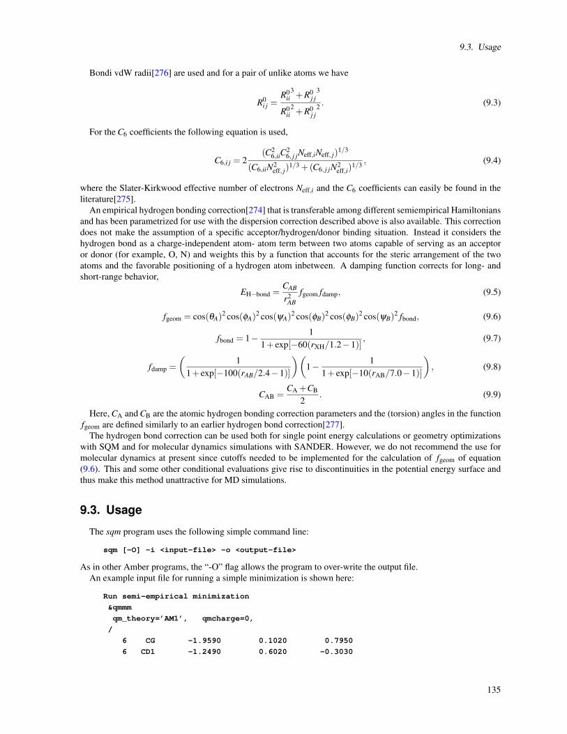
9.3. Usage
Bondi vdW radii[276] are used and for a pair of unlike atoms we have
R0i j =
R0ii
3+R0
j j3
R0ii
2+R0
j j2 . (9.3)
For the C6 coefficients the following equation is used,
C6,i j = 2(C2
6,iiC26, j jNeff,iNeff, j)
1/3
(C6,iiN2eff, j)
1/3 +(C6, j jN2eff,i)
1/3 , (9.4)
where the Slater-Kirkwood effective number of electrons Neff,i and the C6 coefficients can easily be found in theliterature[275].
An empirical hydrogen bonding correction[274] that is transferable among different semiempirical Hamiltoniansand has been parametrized for use with the dispersion correction described above is also available. This correctiondoes not make the assumption of a specific acceptor/hydrogen/donor binding situation. Instead it considers thehydrogen bond as a charge-independent atom- atom term between two atoms capable of serving as an acceptoror donor (for example, O, N) and weights this by a function that accounts for the steric arrangement of the twoatoms and the favorable positioning of a hydrogen atom inbetween. A damping function corrects for long- andshort-range behavior,
EH−bond =CAB
r2AB
fgeom fdamp, (9.5)
fgeom = cos(θA)2 cos(φA)
2 cos(ψA)2 cos(φB)
2 cos(φB)2 cos(ψB)
2 fbond, (9.6)
fbond = 1− 11+ exp[−60(rXH/1.2−1)]
, (9.7)
fdamp =
(1
1+ exp[−100(rAB/2.4−1)]
)(1− 1
1+ exp[−10(rAB/7.0−1)]
), (9.8)
CAB =CA +CB
2. (9.9)
Here, CA and CB are the atomic hydrogen bonding correction parameters and the (torsion) angles in the functionfgeom are defined similarly to an earlier hydrogen bond correction[277].
The hydrogen bond correction can be used both for single point energy calculations or geometry optimizationswith SQM and for molecular dynamics simulations with SANDER. However, we do not recommend the use formolecular dynamics at present since cutoffs needed to be implemented for the calculation of fgeom of equation(9.6). This and some other conditional evaluations give rise to discontinuities in the potential energy surface andthus make this method unattractive for MD simulations.
9.3. Usage
The sqm program uses the following simple command line:
sqm [-O] -i <input-file> -o <output-file>
As in other Amber programs, the “-O” flag allows the program to over-write the output file.An example input file for running a simple minimization is shown here:
Run semi-empirical minimization
&qmmm
qm_theory=’AM1’, qmcharge=0,
/
6 CG -1.9590 0.1020 0.7950
6 CD1 -1.2490 0.6020 -0.3030
135

9. sqm: Semi-empirical quantum chemistry
6 CD2 -2.0710 0.8650 1.9630
6 CE1 -0.6460 1.8630 -0.2340
6 C6 -1.4720 2.1290 2.0310
6 CZ -0.7590 2.6270 0.9340
1 HE2 -1.5580 2.7190 2.9310
16 S15 -2.7820 0.3650 3.0600
1 H19 -3.5410 0.9790 3.2740
1 H29 -0.7870 -0.0430 -0.9380
1 H30 0.3730 2.0450 -0.7840
1 H31 -0.0920 3.5780 0.7810
1 H32 -2.3790 -0.9160 0.9010
The &qmmm namelist contains variables that allow you to control the options used. Following that is one line peratom, giving the atomic number, atom name, and Cartesian coordinates (free format). The variables in the &qmmmnamelist are these:
qm_theory Level of theory to use for the QM region of the simulation (Hamiltonian). Default is to use the semi-empirical Hamiltonian PM3. Options are AM1, RM1, MNDO, PM3-PDDG, MNDO-PDDG, PM3-CARB1, MNDO/d (same as MNDOD), AM1/d (same as AM1D), PM6, and DFTB. The dispersioncorrection can be switched on for AM1 and PM6 by choosing AM1-D* and PM6-D, respectively. Thedispersion and hydrogen bond correction will be applied for AM1-DH+ and PM6-DH+.
dftb_disper Flag turning on (1) or off (0) the use of a dispersion correction to the DFTB/SCC-DFTB energy.Requires qm_theory=DFTB. It is assumed that you have the file DISPERSION.INP_ONCHSP in your$AMBERHOME/dat/slko/ directory. This file must be downloaded from the website www.dftb.org,as described in the beginning of this chapter. Not available for the Zn atom. (Default = 0)
dftb_3rd_order Third order correction to SCC-DFTB. Default=” (the empty string which means no third ordercorrection).
= ’PA’ Use the SCC-DFTB-PA parametrization, which was developed for proton affinities. The pa-rameters will be read from the $AMBERHOME/dat/slko/DFTB_3RD_ORDER_PA.DAT file.
= ’PR’ Use the SCC-DFTB-PR parametrization, which was developed for phosphate hy-drolysis reactions. The parameters will be read from the $AMBERHOME/dat/s-lko/DFTB_3RD_ORDER_PR.DAT file.
= ’READ’ Parameters will be read from the mdin file, in a separate “dftb_3rd_order” namelist, whichmust have the same format as the files above.
= ’filename’ Parameters will be read from the file specified by filename, in the “dftb_3rd_order”namelist, which must have the same format as the files above.
dftb_chg Flag to choose the type of charges to report when doing a DFTB calculation.
= 0 (default) - Print Mulliken charges.
= 2 Print CM3 charges. Only available for H, C, N, O, S and P.
dftb_telec Electronic temperature, in K, used to accelerate SCC convergence in DFTB calculations. The elec-tronic temperature affects the Fermi distribution promoting some HOMO/LUMO mixing, which canaccelerate the convergence in difficult cases. In most cases, a low telec (around 100K) is enough.Should be used only when necessary, and the results checked carefully. Default: 0.0K
dftb_maxiter Maximum number of SCC iterations before resetting Broyden in DFTB calculations. (default: 70 )
qmcharge Charge on the QM system in electron units (must be an integer). (Default = 0)
136

9.3. Usage
spin Multiplicity of the QM system. Currently only singlet calculations are possible and so the defaultvalue of 1 is the only available option. Note that this option is ignored by DFTB/SCC-DFTB, whichallows only ground state calculations. In this case, the spin state will be calculated from the numberof electrons and orbital occupancy.
qmqmdx Flag for whether to calculate QM-QM derivatives analytically or pseudo numerically. The default (andrecommended) option is to use ANALYTICAL QM-QM derivatives.
= 1 (default) - Use analytical derivatives for QM-QM forces.
= 2 Use numerical derivatives for QM-QM forces. Note: the numerical derivative code has not beenoptimised as aggressively as the analytical code and as such is significantly slower. Numericalderivatives are intended mainly for testing purposes.
verbosity Controls the verbosity of QM/MM related output. Warning: Values of 2 or higher will produce a lotof output.
= 0 (default) - only minimal information is printed - Initial QM geometry and link atom positions aswell as the SCF energy at every ntpr steps.
= 1 Print SCF energy at every step to many more significant figures than usual. Also print the numberof SCF cycles needed on each step.
= 2 As 1 but also print info about memory reallocations, number of pairs per QM atom. Also printsQM core - QM core energy, QM core - MM charge energy and total energy.
= 3 As 2 but also print SCF convergence information at every step.
= 4 As 3 but also print forces onof the file QM atoms due to the SCF calculation and the coordinatesof the link atoms at every step.
= 5 As 4 but also print all of the info in kJ/mol as well as kcal/mol.
tight_p_conv Controls the tightness of the convergence criteria on the density matrix in the SCF.
=0 (default) - loose convergence on the density matrix (or Mulliken charges, in case of a SCC-DFTBcalculation). SCF will converge if the energy is converged to within scfconv and the largestchange in the density matrix is within 0.05*sqrt(scfconv).
= 1 Tight convergence on density(or Mulliken charges, in case of a SCC-DFTB calculation). Usesame convergence (scfconv) for both energy and density (charges) in SCF. Note: in the SCC-DFTB case, this option can lead to instabilities.
scfconv Controls the convergence criteria for the SCF calculation, in kcal/mol. In order to conserve energyin a dynamics simulation with no thermostat it is often necessary to use a convergence criterion of1.0d-9 or tighter. Note, the tighter the convergence the longer the calculation will take. Values tighterthan 1.0d-11 are not recommended as these can lead to oscillations in the SCF, due to limitations inmachine precision, that can lead to convergence failures. Default is 1.0d-8 kcal/mol. Minimum usablevalue is 1.0d-14.
pseudo_diag Controls the use of ’fast’ pseudo diagonalisations in the SCF routine. By default the code will attemptto do pseudo diagonalisations whenever possible. However, if you experience convergence problemsthen turning this option off may help. Not available for DFTB/SCC-DFTB.
= 0 Always do full diagonalisation.
= 1 Do pseudo diagonalisations when possible (default).
pseudo_diag_criteria Float controlling criteria used to determine if a pseudo diagonalisation can be done. If thedifference in the largest density matrix element between two SCF iterations is less than this criteriathen a pseudo diagonalisation can be done. This is really a tuning parameter designed for expert useonly. Most users should have no cause to adjust this parameter. (Not applicable to DFTB/SCC-DFTBcalculations.) Default = 0.05
137

9. sqm: Semi-empirical quantum chemistry
diag_routine Controls which diagonalization routine should be used during the SCF procedure. This is an ad-vanced option which has no effect on the results but can be used to fine-tune performance. The speedof each diagonalizer is both a function of the number and type of QM atoms as well as the LAPACKlibrary that Sander was linked to. As such there is not always an obvious choice to obtain the bestperformance. The simplest option is to set diag_routine = 0 in which case Sander will test each diago-nalizer in turn, including the pseudo diagonalizer, and select the one that gives optimum performance.As of AmberTools 15 diag_routine = 0 is now the default for both SQM and QMMM in Sander. Thisshould ideally be the default behavior but this option has not been tested on sufficient architectures tobe certain that it will always work. Not available for DFTB/SCC-DFTB.
= 0 Automatically select the fastest routine (recommended).
= 1 Use internal diagonalization routine (default).
= 2 Use lapack dspev.
= 3 Use lapack dspevd.
= 4 Use lapack dspevx.
= 5 Use lapack dsyev.
= 6 Use lapack dsyevd.
= 7 Use lapack dsyevr.
printcharges
= 0 Don’t print any info about QM atom charges to the output file (default)
= 1 Print Mulliken QM atom charges to output file every ntpr steps.
print_eigenvalues Controls printing of MO eigenvalues.
= 0 Do not print MO eigenvalues
= 1 Print MO eigenvalues at the end of a single point calculation or geometry optimization (default)
= 2 Print MO eigenvalues at the end of every SCF cycle (only NDDO methods, not DFTB)
= 3 Print MO eigenvalues during each step of the SCF cycle (only NDDO methods, not DFTB)
qxd Flag to turn on (=.true.) or off (=.false., default) the charge-dependent exchange-dispersion correctionsof vdW interactions[254].
parameter_file
= ’PARAM.FILE’ Read user-defined parameters from the file ’PARAM.FILE’. The first three space-separated entries (case insensitive) of each line will be interpreted as a user-modified parameterin the sequence of parameter name, element name, and value. For example, a line contains “USSCl -111.6139480D0 “ will cause the USS parameter of the Cl element changed to -111.6139480.A line beginning with “END” will stop the reading. This function currently only works forMNDO, AM1, PM3, MNDO/d, and AM1/d. Also, when new nuclear core-core parameters (FN,in PM3, AM1, and AM1/d) are re-defined, the number of FNN parameter sets (NUM_FN) alsoneeds to be defined. For example, if FNn3 (n = 1, 2, or 3) is defined, then NUM_FN needs to beset to 3 or 4.
peptide_corr
= 0 Don’t apply MM correction to peptide linkages. (default)
= 1 Apply a MM correction to peptide linkages. This correction is of the form Esc f = Esc f +
htype(itype)sin2φ , where φ is the dihedral angle of the H-N-C-O linkage and htype is a constant
dependent on the Hamiltonian used. (Recommended, except for DFTB/SCC-DFTB.)
138

9.3. Usage
itrmax Integer specifying the maximum number of SCF iterations to perform before assuming that conver-gence has failed. Default is 1000. Typically higher values will not do much good since if the SCFhasn’t converged after 1000 steps it is unlikely to. If the convergence criteria have not been met afteritrmax steps the SCF will stop and the minimisation will proceed with the gradient at itrmax. Henceif you have a system which does not converge well you can set itrmax smaller so less time is wastedbefore assuming the system won’t converge. In this way you may be able to get out of a bad geometryquite quickly. Once in a better geometry SCF convergence should improve.
maxcyc Maximum number of minimization cycles to allow, using the xmin minimizer (see Section 40.5) withthe TNCG method. Default is 9999. Single point calculations can be done with maxcyc = 0.
ntpr Print the progress of the minimization every ntpr steps; default is 10.
grms_tol Terminate minimization when the gradient falls below this value; default is 0.02
ndiis_attempts Controls the number of iterations that DIIS (direct inversion of the iterative subspace) extrapola-tions will be attempted. Not available for DFTB/SCC-DFTB. The SCF does not even begin to exhaustits attempts at using DIIS extrapolations until the end of iteration 100. Therefore, for example, ifndiis_attempts=50, then DIIS extrapolations would be performed at end of iterations 100 to 150. Thepurpose of not performing DIIS extrapolations before iteration 100 is because the existing code baseperforms quite well for most molecules; however, if convergence is not met after 100 iterations, then itis presumed that further iterations will not yield SCF convergence without doing something different,i.e., DIIS. Thus, the implementation of DIIS in SQM is a mechanism to try and force SCF conver-gence for molecules that are otherwise difficult to converge. Default 0. Maximum 1000. Minimum0. Note that DIIS will automatically turn itself on for 100 attempts at the end of iteration 800 even ifyou did not explicitly set ndiis_attempts to a nonzero value. This is done as a final effort to achieveconvergence.
ndiis_matrices Controls the number of matrices used in the DIIS extrapolation. Including only one matrix is thesame as not performing an extrapolation. Including an excessive number of matrices may require alarge amount of memory. Not available for DFTB/SCC-DFTB. Default 6. Minimum 1. Maximum 20.
vshift Controls level shifting (only NDDO methods, not DFTB). Virtual orbitals can be shifted up by vshift(in eV) to improve SCF convergence in cases with small HOMO/LUMO gap. Default 0.0 (no levelshift).
errconv SCF tolerance on the maximum absolute value of the error matrix, i.e., the commutator of the Fockmatrix with the density matrix. The value has units of hartree. The default value of errconv is suffi-ciently large to effectively remove this tolerance from the SCF convergence criteria. Not available forDFTB/SCC-DFTB. Default 1.d-1. Minimum 1.d-16. Maximum 1.d0.
qmmm_int When running QM calculations in the sqm program, an electric field of external point charges canbe added. In this way, the electrostatic effect outside of the QM region can be modeled, making thecalculation a simplified QM/MM calculation without QM/MM vdW’s contribution. Like QM/MMcalculations (see Section 10), the method to couple QM and MM electrostatic interactions for externalcharges and semiempirical Hamiltonians can be specified via the qmmm_int namelist variable.
The current implementation limits use of external charges to only single point energy calculations. Torun such a calculation, an additional field, which begins with #EXCHARGES and ends with #END,is required to specify the external point charges in the input. Each external point charge must includeatomic number, atom name, X, Y, Z coordinates and the charge in units of the electron charge. Anexample input looks like:
single point energy calculation (adenine), with external charges (thymine)
&qmmm
qm_theory = ’PM3’,
qmcharge = 0,
139

9. sqm: Semi-empirical quantum chemistry
maxcyc = 0,
qmmm_int = 1,
/
7 N 1.0716177 -0.0765366 1.9391390
1 H 0.0586915 -0.0423765 2.0039181
1 H 1.6443796 -0.0347395 2.7619159
6 C 1.6739638 -0.0357766 0.7424316
7 N 0.9350155 -0.0279801 -0.3788916
6 C 1.5490760 0.0012569 -1.5808009
1 H 0.8794435 0.0050260 -2.4315709
7 N 2.8531510 0.0258031 -1.8409596
6 C 3.5646109 0.0195446 -0.7059872
6 C 3.0747955 -0.0094480 0.5994562
7 N 4.0885824 -0.0054429 1.5289786
6 C 5.1829921 0.0253971 0.7872176
1 H 6.1882591 0.0375542 1.1738824
7 N 4.9294871 0.0412404 -0.5567274
1 H 5.6035368 0.0648755 -1.3036811
#EXCHARGESwill be
6 C -4.7106131 0.0413373 2.1738637 -0.03140
1 H -4.4267056 0.9186178 2.7530256 0.06002
1 H -4.4439282 -0.8302573 2.7695655 0.05964
1 H -5.7883971 0.0505530 2.0247280 0.03694
6 C -3.9917387 0.0219348 0.8663338 -0.25383
6 C -4.6136833 0.0169051 -0.3336520 0.03789
1 H -5.6909220 0.0269347 -0.4227183 0.16330
7 N -3.9211729 -0.0009646 -1.5163659 -0.47122
1 H -4.4017172 -0.0036078 -2.4004924 0.35466
6 C -2.5395897 -0.0149474 -1.5962357 0.80253
8 O -1.9416783 -0.0291878 -2.6573783 -0.63850
7 N -1.9256484 -0.0110593 -0.3638948 -0.58423
1 H -0.8838255 -0.0216168 -0.3784269 0.35404
6 C -2.5361367 0.0074651 0.8766724 0.71625
8 O -1.8674730 0.0112093 1.9120833 -0.60609
#END
140

10. QM/MM calculations
Sander supports the option of describing part of the system quantum mechanically in an approach known as ahybrid (or coupled potential) QM/MM simulation. Semi-empirical neglect of diatomic overlap (NDDO)-type anddensity functional tight binding (DFTB) Hamiltonians are supported natively by sander and the basic documen-tation (e.g. what Hamiltonians are implemented, description of the input parameters) can be found in Chapter 9.Here we limit our description to those features that are unique to the QM/MM interface implemented in sander.More advanced Hamiltonians based on ab initio wave function theory (WFT) and density functional theory (DFT)are supported via an interface to external QM software packages the use of which is described in section 10.2.
The built-in semi-empirical QM/MM support was written by Ross Walker and Mike Crowley, [250] basedoriginally on public-domain MOPAC codes of J.J.P. Stewart. The QM/MM generalized Born implementation usesthe model described by Pellegrini and Field[278] while regular QM/MM Ewald support is based on the workof Nam et al.[279] with QM/MM PME support based on the work of Walker et al.[250]. SCC-DFTB supportwas written by Gustavo Seabra, Ross Walker and Adrian Roitberg,[251] and is based on earlier work of MarcusElstner.[252, 253] Support for third-order SCC-DFTB was written by Gustavo Seabra and Josh McClellan.
10.1. Built-in semiempirical NDDO methods and SCC-DFTB
When running a QM/MM simulation in sander the system is partitioned into two regions, a QM region consistingof the atoms defined by either the qmmask or iqmatoms keyword, and a MM region consisting of all the atoms thatare not part of the QM region. For a typical protein simulation in explicit solvent the number of MM atoms willbe much greater than the number of QM atoms. Either region can contain zero atoms, giving either a pure QMsimulation or a standard classical simulation. For periodic simulations, the quantum region must be compact, sothat the extent (or diameter) of the QM region (in any direction) plus twice the QM/MM cutoff must be less thanthe box size. Hence, you can define an "active site" to be the QM region, but in most cases could not ask thatall cysteine residues (for example) be quantum objects. The restrictions are looser for non-periodic (gas-phaseor generalized Born) simulations, but the codes are written and tested for the case of a single, compact quantumregion.
The partitioned system is characterized by an effective Hamiltonian which operates on the system’s wavefunc-tion Ψ, which is dependent on the position of the MM and QM nuclei, to yield the system energy Ee f f :
He f f Ψ(xe,xQM,xMM) = Ee f f (xQM,xMM)Ψ(xe,xQM,xMM) (10.1)
The effective Hamiltonian consists of three components - one for the QM region, one for the MM region and aterm that describes the interaction of the QM and MM regions, implying that likewise the energy of the system canbe divided into three components. If the total energy of the system is re-written as the expectation value of He f fthen the MM term can be removed from the integral since it is independent of the position of the electrons:
Ee f f =⟨Ψ|HQM +HQM/MM|Ψ
⟩+EMM (10.2)
In the QM/MM implementation in sander, EMM is calculated classically from the MM atom positions usingthe Amber or CHARMM force field equation and parameters, whereas HQM is evaluated using the chosen QMmethod.
The interaction term HQM/MM is more complicated. By default, sander uses an electrostatic embedding scheme(also referred to as additive scheme) in which the interaction of the MM point charges with the electrons of theQM system as well as the interaction between the MM point charges and the QM nuclei (atomic cores for semi-empirical methods) is explicitly taken into account. In other words, the MM region polarizes the QM electrondensity. For the case where there are no covalent bonds between the atoms of the QM and MM regions the
141

10. QM/MM calculations
interaction Hamiltonian is thus the sum of an electrostatic term and a Lennard-Jones (VDW) term and can bewritten as
HQM/MM = ∑q
∑m
[Qmhelectron(xe,xMM)−QmZqhcore(xQM,xMM)+
(A
r12qm− B
r6qm
)](10.3)
where the subscripts e, m and q refer to the electrons, the MM nuclei and the QM nuclei respectively. Here Qm isthe charge on MM atom m, Zq is the core charge (nucleus minus core electrons) on QM atom q, rqm is the distancebetween atoms q and m, and A and B are Lennard-Jones interaction parameters. For systems that have covalentbonds between the QM and MM regions, the situation is more complicated, as discussed later.
A more approximate form of the interaction term HQM/MM is referred to as mechanical embedding (or subtractiveQM/MM scheme). In this case the interactions between the QM and the MM region are obtained within the sameclassical approximation that is used for the MM region, that is
HQM/MM = ∑q
∑m
[QmQq
rqm+
(A
r12qm− B
r6qm
)](10.4)
where Qq is the classical MM point charge assigned to an atom in the QM region. Mechanical embedding is usefulto impose steric constraints on the embedded QM system, however, the electron density is not polarized by theMM environment. An additional complication of this approach is that the point charges that are assigned to theatoms in the QM region have to represent the electrostatic potential of the QM region during the whole course ofa QM/MM simulation.
If one evaluates the expectation values in Eq. 10.2 over a single determinant built from molecular orbitals
φi = ∑j
ci jχ j (10.5)
where the ci j are molecular orbital coefficients and the χ j are atomic basis functions, the total energy depends uponthe ci j and on the positions xMM and xQM of the atoms. The energy is obtained by setting ∂Ee f f /∂ci j to zero whichleads to a self-consistent (SCF) procedure to determine the ci j, (with a modified Fock matrix that contains theelectric field arising from the MM charges in the case of electrostatic embedding). Once the energy is known, theforces on the atoms can be obtained by taking the derivative of the energy expression with respect to the positionsof the QM and MM atoms.
The main subtlety that arises in the case of electrostatic embedding is that, for a periodic system, there areformally an infinite number of QM/MM interactions; even for a non-periodic system, the (finite) number of suchinteractions may be prohibitively large. These problems are addressed in a manner analogous to that used for pureMM systems: a PME approach is used for periodic systems, and a (large) cutoff may be invoked for non-periodicsystems. Some details are discussed below.
10.1.1. The QM/MM interface and link atoms
The sections above dealt with situations where there are no covalent bonds between the QM and MM regions. Inmany protein simulations, however, it is necessary to have the QM/MM boundary cut covalent bonds, and a numberof additional approximations have to be made. There are a variety of approaches to this problem, including hybridorbitals, capping potentials, and explicit link atoms. The last option is the method available in sander.
There are a number of ways to implement a link atom approach that deal with the way the link atom is positioned,the way the forces on the link atom are propagated, and the way non-bonding interactions around the link atom aretreated. Each time an energy or gradient calculation is to be done, the link atom coordinates are re-generated fromthe current coordinates of the QM and MM atoms making up the QM-MM covalent pair. The link atom is placedalong the bond vector joining the QM and MM atom, at a distance dL−QM from the QM atom. By default dL−QM isset to the equilibrium distance of a methyl C-H atom pair (1.09 Å) but this can be set in the input file. The defaultlink atom type is hydrogen, but this can also be specified as an input.
Since the link atom position is a function of the coordinates of the "real" atoms, it does not introduce any newdegrees of freedom into the system. The chain rule is used to re-write forces on the link atom itself in terms
142

10.1. Built-in semiempirical NDDO methods and SCC-DFTB
of forces on the two real atoms that define its position. This is analogous to the way in which "extra points" or"lone-pairs" are handled in MM force fields.
The remaining details of how the QM-MM boundary is treated are as follows: for the interactions surroundingthe link atom, the MM bond term between the QM and MM atoms is calculated classically using the classicalforce field parameters, as are any angle or dihedral terms that include at least one MM atom. The Lennard-Jonesinteractions between QM-MM atom pairs are calculated in the same way as described in the section above withexclusion of 1-2 and 1-3 interactions and scaling of 1-4 interactions. What remains is to specify the electrostaticinteractions between QM and MM atoms around the region of the link atom.
A number of different schemes have been proposed for handling link-atom electrostatics. Many of these havebeen tested or calibrated on (small) gas-phase systems, but such testing can neglect some considerations that arevery important for more extended, condensed-phase simulations. In choosing our scheme, we wanted to ensurethat the total charge of the system is rigorously conserved (at the correct value) during an MD simulation. Further,we strove to have the Mulliken charge on the link atom (and the polarity of its bond to the nearest QM atom)adopt reasonable values and to exhibit only small fluctuations during MD simulations. Link atoms interact withthe MM field in exactly the same way as regular QM atoms. That is they interact with the electrostatic field dueto all the MM atoms that are within the cutoff, with the exception of the MM link pair atoms (MM atoms that arebound directly to QM atoms). VDW interactions are not calculated for link atoms. These are calculated betweenall real QM atoms and all MM atoms, including the MM link pair atoms. For Generalized Born simulations theeffective Born radii for the link atoms are calculated using the intrinsic radii for the MM link pair atoms that theyare replacing.
In the case of electrostatic embedding the atoms that make up the QM region (including the MM link pairatom) have their charges from the prmtop file essentially replaced with Mulliken charges. Hence it is important toconsider the issue of charge conservation. The QM region (including the link atoms) by definition must have aninteger charge. This is defined by the &qmmm namelist variable qmcharge. If the MM atoms (including the MMlink pair atoms) that make up the QM region have prmtop charges that sum to the value of qmcharge then there isno problem. If not, there are two options for dealing with this charge, defined by the namelist variable adjust_q. Avalue of 1 will distribute the difference in charge equally between the nearest nlink MM atoms to the MM link pairatoms. A value of 2 will distribute this charge equally over all of the MM atoms in the simulation (excluding MMlink pair atoms).
10.1.2. A reformulated QM/MM interface for PM3
In the current version of Amber, a reformulated QM-MM core-charge potential (denoted as PM3/MM*) hasbeen implemented. This reformulated potential scales the interaction between a QM core and a MM charge for thepurpose of better description of the geometry and energy at the QM-MM interface:[280]
EcoreQM/MM = Zaqm (sasa,smsm)
[1+|qm|qm·(−e− f a
1 ·Ram + e− f a2 ·Ram
)](10.6)
where Za is the effective core charge of QM atom a, qm is the partial charge on MM atom m, sa is an s orbitalon the QM atom, sm is a notional s orbital on the MM atom, Ram is the QM-MM interatomic distance, and f a
1and f a
2 are exponential scale factors which depend on the QM atom only. Optimal values for f a1 and f a
2 weredetermined based on the PM3 Hamiltonian, and are available for H, C, N and O atoms (so the QM region islimited to these four atoms; but the MM region is not restricted). Application of this reformulated potential showsimproved prediction of geometry and interaction energy at the QM-MM interface for hydrogen bonded smallmolecule complexes typical of biomolecular interactions, without significantly impacting the modeling of otherinteraction types, such as dispersion dominant complexes.[280] In a QM/MM calculation, giving qmmm_int=3along with qm_theory=PM3 will invoke this potential.
Based on PM3/MM*, further developments to the semi-empirical QM/MM coupling method have been intro-duced – PM3/MMX2 (qmmm_int=4 and qm_theory=PM3) – which shares the same QM core-MM charge equationwith the PM3/MM* model. In addition, a QM parameter, ρmm, is introduced to each type of QM atoms in orderto "fine-tune" the QM electron-MM charge interaction (Eq. 10.7). Although ρmm is a parameter for QM atom, thesubscript mm emphasizes that it is a MM-related property (eqn 3.xx). Parameters are currently avaiable for H, C,N, O and S QM atoms (manuscript in preparation).
143

10. QM/MM calculations
EelectronQM/MM =−qm(µaνa,smsm) = ∑
`a
∑`m
[Ma
lakMmlmk]
(10.7)
where
[Ma
lakMmlmk]=
e2
2la+lm
2la
∑i=1
l
∑j=1
[r2
i j +(ρ
ala+ρ
amm)2]−1/2
(10.8)
10.1.3. Generalized Born implicit solvent
The implementation of Generalized Born (GB) for QM/MM calculations is based on the method described byPellegrini and Field.[278] Here, the total energy is taken to be Ee f f from Eq. 10.2 plus Egb from Eq. 4.2. In Egb,charges on the QM atoms are taken to be the Mulliken charges determined from the quantum calculation; hencethese charges depend upon the molecular orbital coefficients ci j as well as the positions of the atoms.
As with conventional QM/MM simulations, one then solves for the ci j by setting ∂Ee f f /∂ci j = 0. This leadsto a set of SCF equations with a Fock matrix modified not only by the presence of MM atoms (as in "ordinary"QM/MM simulations), but also modified by the presence of the GB polarization terms. Once self-consistency isachieved, the resulting Mulliken charges can be used in the ordinary way to compute the GB contribution to thetotal energy and forces on the atoms.
10.1.4. Ewald and PME
The support for long range electrostatics in QM/MM calculations using electrostatic embedding is based on amodification of the Nam, Gao and York Ewald method for QM/MM calculations.[279] This approach works in asimilar fashion to GB in that Mulliken charges are used to represent long range interactions. Within the cut off,interactions between QM and MM atoms are calculated using a full multipole treatment. Outside of the cut off theinteraction is based on pairwise point charge interactions. For semiempirical NDDO-type methods this leads to aslight discontinuity at the QM/MM cut off boundary and thus a small energy drift during QM/MM MD simulationsin the NVE ensemble. This energy drift can be avoided by using a switching function at the cutoff (see below).
The implementation in Ref [279] uses an Ewald sum for both QM/QM and QM/MM electrostatic interactions.This can be expensive for large MM regions, and thus sander uses a modification of this method by Walker andCrowley[250] that uses a PME model (rather than an Ewald sum) for QM/MM interactions. This is controlled bythe qm_pme variable discussed below.
When running QM/MM Ewald or PME simulations in sander, if QM multipoles are involved in QM-MMinteractions (NDDO methods), a discontinuity in the QM-MM electrostatic potential occurs at the cut-off distancedue to the sudden change in the potential function (the difference between Eqs. 10.9 and 10.10) , thus resulting inenergy conservation problems in the simulation.
Er<cuto f fQM/MM =−qm(µaνa,smsm)+Zaqm(sasa,smsm)(1+ scale) (10.9)
Er>cuto f fQM/MM =
qm(Za−∑cµµ)
r(10.10)
This problem can be avoided by applying a switching function to smoothly connect the two different potentials.The QM/MM electrostatic potential using a switching function can thus be written as:
EQM/MM = Er<cuto f fQM/MM s(r)+Er>cuto f f
QM/MM (1− s(r))
The switching function can be turned on or off via the &qmmm namelist variable qmmm_switch, for details seesection 10.1.6 below.
144

10.1. Built-in semiempirical NDDO methods and SCC-DFTB
10.1.5. Hints for running successful QM/MM calculations
Required Parameters and Prmtop Creation
QM/MM calculations without link atoms require mass, charges, van der Waals and GB radii in the prmtopfile. All bonds, angles, and dihedrals parameters involving QM atoms are neglected. In the case of electrostaticembedding the charges are also neglected. (Note that when SHAKE is applied to the QM reg, the bonds areconstrained to the ideal MM values, even when these are part of a QM region; hence, for this case, it is importantto have correct bond parameters in the QM region.) The simplest general prescription for setting things up is touse antechamber and LEaP to create a reference force field, since "placeholders" are required in the prmtop fileeven for things that will be neglected. This also allows you to run comparison simulations between pure MM andQM/MM simulations, which can be helpful if problems are encountered in the QM/MM calculations.
The use of antechamber to construct a pure MM reference system is even more useful when there are link atoms,since here MM parameters for bonds, angles and dihedrals that cross the QM/MM boundary are also needed.
Choosing the QM region
There are no good universal rules here. Generally, one might want to have as large a QM region as possible,but having more than 80-100 atoms in the QM region will lead to simulations that are very expensive. One shouldalso remember that for many features of conformational analysis, a good MM force field may be better than asemiempirical or DFTB quantum description. In choosing the QM/MM boundary, it is better to cut non-polarbonds (such as C-C single bonds) than to cut unsaturated or polar bonds. Link atoms are not placed between bondsto hydrogen. Thus cutting across a C-H bond will NOT give you a link atom across that bond. (This is not currentlytested for in the code and so it is up to the user to avoid such a situation.) Furthermore, link atoms are restrictedto one per MM link pair atom. This is tested for during the detection of link atoms and an error is generated ifthis requirement is violated. This would seem to be a sensible policy otherwise you could have two link atoms tooclose together. See the comments in qm_link_atoms.f for a more in-depth discussion of this limitation.
Choice of electrostatic cutoff
The implementation of the non-bonded cut off in QM/MM simulations is slightly different than in regular MMsimulations. The cut off between MM-MM atoms is still handled in a pairwise fashion. However, for QM atomsany MM atom that is within qmcut of ANY QM atom is included in the interaction list for all QM atoms. Thismeans that the value of qmcut essentially specifies a shell around the QM region rather than a spherical shellaround each individual QM atom. Ideally the cut off should be large enough that the energy as a function of thecutoff has converged. For non-periodic, generalized Born simulations, a cutoff of 15 to 20 Å seems sufficient insome tests. (Remember that long-range electrostatic interactions are reduced by a factor of 80 from their gas-phasecounterparts, and by more if a nonzero salt concentration is used.) For periodic simulations, the cutoff only servesto divide the interactions between "direct" and "reciprocal" parts; as with pure MM calculations, a cutoff of 8 or 9Å is sufficient here.
Parallel simulations
The built-in QM/MM implementation currently supports execution in parallel via the message passing interface(MPI), however, the implementation is not fully parallel. At present all parts of the QM simulation are parallelexcept the density matrix build and the matrix diagonalisation. For small QM systems these two operations donot take a large percentage of time and so acceptable scaling can be seen to around 8 CPU cores (depending ontype of CPU and/or interconnect speed between compute nodes). For large QM systems the matrix diagonalisationtime will dominate and so the scaling will not be as good. In this case it may be beneficial to choose a LAPACKdiagonalization routine in combination with a threaded library such as the Intel Math Kernel Library (MKL). Fordetails on how to choose the diagonalization routine see Section 9.3. The number of threads to be used for thediagonalization is set via an environment variable of the operating system (typically OMP_NUM_THREADS).
145

10. QM/MM calculations
10.1.6. General QM/MM &qmmm Namelist Variables
An example input file for running a simple QM/MM MD simulation is shown here: &cntrl
imin=0, nstlim=10000, ! Perform MD for 10,000 steps
dt=0.002, ! 2 fs time step
ntt=1, tempi=0.1, temp0=300.0, ! Berendsen temperature control
ntb=1, ! Constant volume periodic boundaries
ntf=2, ntc=2, ! Shake hydrogen atoms
cut=8.0, ! 8 angstrom classical non-bond cut off
ifqnt=1 ! Switch on QM/MM coupled potential
/
&qmmm
qmmask=’:753’, ! Residue 753 should be treated using QM
qmcharge=-2, ! Charge on QM region is -2
qm_theory=’PM3’, ! Use the PM3 semi-empirical Hamiltonian
qmcut=8.0 ! Use 8 angstrom cut off for QM region
/ The &qmmm namelist contains variables that allow you to control the options used for a QM/MM simulation. Thisnamelist must be present when running QM/MM simulations and at the very least must contain either the iqmatomsor qmmask variable which define the region to be treated quantum mechanically. If ifqnt is set to zero then thecontents of this namelist are ignored.
For the QM region definition specify one of either iqmatoms or qmmask. Link atoms will be added automaticallyalong bonds (as defined in the prmtop file) that cross the QM/MM boundary.
iqmatoms comma-separated integer list containing the atom numbers (from the prmtop file) of the atoms to betreated quantum mechanically.
qmmask Mask specifying the quantum atoms. E.g. :1-2, = residues 1 and 2. See mask documentation for moreinfo.
qmcut Specifies the size of the electrostatic cutoff in Angstroms for QM/MM electrostatic interactions. Bydefault this is the same as the value of cut chosen for the classical region, and the default generallydoes not need to be changed. Any classical atom that is within qmcut of any QM atom is included inthe pair list. For PME calculations, this parameter just affects the division of forces between direct andreciprocal space. Note: this option only effects the electrostatic interactions between the QM and MMregions. Within the QM region all QM atoms see all other QM atoms regardless of their separation.QM-MM van der Waals interactions are handled classically, using the cutoff value specified by cut.
qm_ewald This option specifies how long range electrostatics for the QM region should be treated.
= 0 Use a real-space cutoff for QM-QM and QM-MM long range interactions. In this situation QMatoms do not see their images and QM-MM interactions are truncated at the cutoff. This is thedefault for non-periodic simulations.
= 1 (default) Use PME or an Ewald sum to calculate long range QM-QM and QM-MM electrostaticinteractions. This is the default when running QM/MM with periodic boundaries and PME.
= 2 This option is similar to option 1 but instead of varying the charges on the QM images as thecentral QM region changes the QM image charges are fixed at the Mulliken charges obtainedfrom the previous MD step. This approach offers a speed improvement over qm_ewald=1, sincethe SCF typically converges in fewer steps, with only a minor loss of accuracy in the long rangeelectrostatics. This option has not been extensively tested, although it becomes increasinglyaccurate as the box size gets larger.
146
10.1. Built-in semiempirical NDDO methods and SCC-DFTB
kmaxqx,y,z Specifies the maximum number of kspace vectors to use in the x, y and z dimensions respectively whendoing an Ewald sum for QM-MM and QM-QM interactions. Higher values give greater accuracy inthe long range electrostatics but at the expense of calculation speed. The default value of 8 should beoptimal for most systems.
ksqmaxq Specifies the maximum number of K squared values for the spherical cut off in reciprocal space whendoing a QM-MM Ewald sum. The default value of 100 should be optimal for most systems.
qm_pme Specifies whether a PME approach or regular Ewald approach should be used for calculating the longrange QM-QM and QM-MM electrostatic interactions.
= 0 Use a regular Ewald approach for calculating QM-MM and QM-QM long range electrostatics.Note this option is often much slower than a pme approach and typically requires very largeamounts of memory. It is recommended only for testing purposes.
= 1 (default) Use a QM compatible PME approach to calculate the long range QM-MM electrostaticenergies and forces and the long range QM-QM forces. The long range QM-QM energies arecalculated using a regular Ewald approach.
qmmm_switch Specifies whether a switching function shall be used at the cutoff for long range electrostatics(applies only to NDDO methods). The lower and higher boundaries of the switching function are userdefinable, see r_switch_lo and r_switch_hi.
= 0 (default). Do not use a switching function. This leads to slight discontinuities in the potential atthe cut off and thus an energy drift in NVE simulations.
= 1 Use a switching function. See also variables r_switch_hi and r_switch_lo.
r_switch_hi Specifies the upper boundary of the switching function in Å (see qmmm_switch). Defaults to qmcut.
r_switch_lo Specifies lower boundary of the switching function in Å (see qmmm_switch). Defaults to r_switch_hi- 2.
qmgb Specifies how the QM region should be treated with generalized Born.
= 2 (default) As described above, the electrostatic and "polarization" fields from the MM charges andthe exterior dielectric (respectively) are included in the Fock matrix for the QM Hamiltonian.
= 3 This is intended as a debugging option and should only be used for single point calculations. Withthis option the GB energy is calculated using the Mulliken charges as with option 2 above but thefock matrix is NOT modified by the GB field. This allows one to calculate what the GB energywould be for a given structure using the gas phase quantum charges. When combined with asimulation using qmgb=2, this allows the strain energy from solvation to be calculated.
qm_theory Level of theory to use for the QM region of the simulation. (Hamiltonian). Default is to use thesemi-empirical hamiltonian PM3. See the Section 9.3 for details.
qmmm_int Controls the way in which QM/MM interactions are handled in the direct space QMMM sum. Thiscontrols only the electrostatic interactions. VDW interactions are always calculated classically us-ing the standard 6-12 potential. Note: with the exception of qmmm_int=0 DFTB calculations(qm_theory=DFTB) always use a simple mulliken charge - resp charge interaction and the value ofqmmm_int has no influence.
= 0 This turns off all electrostatic interaction between QM and MM atoms in the direct space sum.Note QM-MM VDW interactions will still be calculated classically.
= 1 (default) QM-MM interactions in direct space are calculated in the same way for all of the varioussemi-empirical hamiltonians. The interaction is calculated in an analogous way to the the core-core interaction between QM atoms. The MM resp charges are included in the one electronhamiltonian so that QMcore-MMResp and QMelectron-MMResp interactions are calculated.
147
10. QM/MM calculations
= 2 This is the same as for 1 above except that when AM1, PM3 or Hamiltonians derived from theseare in use the extra Gaussian terms that are introduced in these methods to improve the core-corerepulsion term in QM-QM interactions are also included for the QM-MM interactions. This isthe equivalent to the QM-MM interaction method used in CHARMM and DYNAMO. It tendsto slightly reduce the repulsion between QM and MM atoms at small distances. For distancesabove approximately 3.5 angstroms it makes almost no difference.
= 3 Using this along with qm_theory=PM3 invokes a reformulated QM core-MM charge potential atthe QM-MM interface (Eq. 10.6). Current parametrization limits the QM region to H, C, N andO atoms only; MM region is not restricted.[280]
= 4 Currently not in use.
= 5 Mechanical embedding: The electrostatic interaction between QM and MM atoms is treated onthe same level as within the MM region using the classical force field point charges also for theQM atoms. The electronic Hamiltonian does not contain the field generated by the MM regionpoint charges and thus the electron density is not polarized by the MM environment. Does notwork with GB. Not extensively tested in presence of link atoms.
qmshake Controls whether SHAKE is applied to QM atoms. Using SHAKE on the QM region will allow youto use larger time steps such as 2 fs with NTC=2. If, however, you expect bonds involving hydrogento be broken during a simulation you should not SHAKE for the QM region. WARNING: the SHAKEroutine uses the equilibrium bond lengths as specified in the prmtop file to reset the atom positions.Thus while bond force constants and equilibrium distances are not used in the energy calculation forQM atoms the equilibrium bond length is still required if QM SHAKE is on.
= 0 Do not shake QM H atoms.
= 1 Shake QM H atoms if SHAKE is turned on (NTC>1) (default).
printdipole Controls whether the dipole moment shall be printed every ntpr steps.
= 0 Do not print the dipole moment (default).
= 1 Print the dipole moment of the QM region.
= 2 Print the total dipole moment of the QM and MM region.
writepdb
= 0 Do not write a PDB file of the selected QM region. (default).
= 1 Write a PDB file of the QM region. This option is designed to act as an aid to the user to allow easychecking of what atoms were included in the QM region. When this option is set a crude PDB fileof the atoms in the QM region will be written on the very first step to the file qmmm_region.pdb.
vsolv Controls whether solvent molecules shall be included into the QM region (requires settings in the&vsolv namelist; see also section 10.3 on adaptive solvent QM/MM simulations, in particular thenamelist information in section 10.3.2.2).
= 0 Do not include solvent molecules into the QM region (default).
= 1 Include solvent molecules via simple solvent switching (requires &vsolv namelist).
= 2 Adaptive solvent QM/MM with fixed number of solvent molecules in A and T regions (requires&vsolv and &adqmmm namelists).
= 3 Adaptive solvent QM/MM with fixed size of A and T regions (requires &vsolv and &adqmmmnamelists).
In addition to the above parameters, the following variables may be set, as described in Section 9.3:qm_theory, dftb_disper, dftb_3rd_order , dftb_chg , dftb_telec , dftb_maxiter , qmcharge, spin, qmqmdx, ver-
bosity, tight_p_conv, scfconv, pseudo_diag, pseudo_diag_criteria, diag_routine, printcharges, qxd, parameter_file,peptide_corr, and itrmax.
148

10.1. Built-in semiempirical NDDO methods and SCC-DFTB
10.1.7. Link Atom Specific QM/MM &qmmm Namelist Variables
The following options go in the &qmmm namelist and control the link atom behaviour.
lnk_dis Distance in Å from the QM atom to its link atom. Currently all link atoms must be placed at thesame distance. A negative value of lnk_dis specifies that the link atom should be placed directly ontop of the MM link pair atom. In this case the distance of the link atom from the QM region changesas a function of time and the actual value of lnk_dis is ignored. Additionally this means that not alllink atoms will be placed at the same distance. Negative values of lnk_dis will work with regularlink atoms, such as hydrogen, but are really intended for use with pseudo atom / capping approaches.Default = 1.09Å.
lnk_method This defines how classical valence terms that cross the QM/MM boundary are dealt with.
=1 (Default) in this case any bond, angle or dihedral that involves at least one MM atom, includingthe MM link pair atom is included. This means the following (where QM = QM atom, MM =MM atom, MML = MM link pair atom.):
Bonds = MM-MM, MM-MML, MML-QM
Angles = MM-MM-MM, MM-MM-MML, MM-MML-QM, MML-QM-QM
Dihedrals = MM-MM-MM-MM, MM-MM-MM-MML, MM-MM-MM-MML-QM, MM-MML-QM-QM, MML-QM-QM-QM
=2 Only include valence terms that include a full MM atom, that is, count the MM link pair atom aseffectively being a QM atom. This option is designed to be used in conjunction with a pseudoatom / capping type approach where the link atom is parameterized specifically to behave like auni-valent version of the MM atom it replaces. This option gives the following interactions:
Bonds = MM-MM, MM-MML
Angles = MM-MM-MM, MM-MM-MML, MM-MML-QM
Dihedrals = MM-MM-MM-MM, MM-MM-MM-MML, MM-MM-MML-QM, MM-MML-QM-QM
lnk_atomic_no The atomic number of the link atoms. This selects what element the link atoms are to be. Default= 1 (Hydrogen). Note this must be an integer and an atomic number supported by the chosen QMtheory.
adjust_q This controls how charge is conserved during a QMMM calculation involving link atoms. When theQM region is defined the QM atoms and any MM atoms involved in link bonds have their RESPcharges zeroed. If the sum of these RESP charges does not exactly match the value of qmcharge thenthe total charge of the system will not be correct.
= 0 No adjustment of the charge is done.
= 1 The charge correction is applied to the nearest nlink MM atoms to MM atoms that form link pairs.Typically this will be any MM atom that is bonded to a MM link pair atom (a MM atom thatis part of a QM-MM bond). This results in the total charge of QM+QMlink+MM equaling theoriginal total system charge from the prmtop file. Requires natom-nquant-nlink >= nlink andnlink>0.
= 2 (default) - This option is similar to option 1 but instead the correction is divided among all MMatoms (except for those adjacent to link atoms). As with option 1 this ensures that the total chargeof the QM/MM system is the same as that in the prmtop file. Requires natom-nquant-nlink >=nlink.
149

10. QM/MM calculations
10.1.8. Charge-dependent exchange-dispersion corrections of vdW interactions
The sqm program provides a new charge-dependent energy model consisting of van der Waals (vdW) and polar-ization interactions between the quantum mechanical (QM) and molecular mechanical (MM) regions in a combinedQM/MM calculation. vdW interactions are commonly treated using empirical Lennard-Jones (L-J) potentials,whose parameters are often chosen based on the QM atom type (e.g., based on hybridization or specific covalentbonding environment). This strategy for determination of QM/MM nonbonding interactions becomes tedious toparametrize and lacks robust transferability. Problems occur in the study of chemical reactions where the "atomtype" is a complex function of the reaction coordinate. This is particularly problematic for reactions, where atomsor localized functional groups undergo changes in charge state and hybridization.
In sqm, this charge-dependent energy model was implemented based on a scaled overlap model for repulsiveexchange and attractive dispersion interactions that is a function of atomic charge. The model is chemicallysignificant since it properly correlates atomic size, softness, polarizability, and dispersion terms with minimalone-body parameters that are functions of the atomic charge[254].
This “Charge-dependent exchange-dispersion corrections of vdW interactions” can be invoked by the“qxd=.true.” switch in the &qmmm namelist. Note that this model currently does not have any effect on purequantum calculations through sqm, the qxd correction is only added to QM/MM interactions in sander. The de-fault values of qxd parameters are set to reproduce the regular L-J interactions of typical atom types (HC for H,C* for C, N for N, OW for O, and parameters for F and Cl are optimized[254]) when the charge dependenceparameters are zero. There are eight qxd parameters (symbols used in the reference[254] are indicated in theparentheses): qxd_s (s), qxd_z0 (ζ (0)), qxd_zq (ζq), qxd_d0 (α1), qxd_dq (3×B), qxd_q0 (α2), qxd_qq (3×B),and qxd_neff (Ne f f (0)). All parameters can be modified through external user-defined parameter files (see theusage of ’parameter_file’ in Section 9.3).
10.2. Interface for ab initio and DFT methods
In addition to the built-in semi-empirical methods sander also supports QM/MM simulations with ab initio wavefunction theory (WFT) and density functional theory (DFT) potentials via an interface to external QM softwarepackages[281]. The implementation makes use of the existing QM/MM infrastructure that has been developedearlier for the semi-empirical methods. Thus, much of AMBER’s previous QM/MM functionality such as the user-friendly link atom approach are available and the implementation remains simple and transparent to use withoutany significant additional steps in the simulation setup as compared to semi-empirical QM/MM simulations. Atpresent the interface supports several well-known and widely used QM software packages. Mechanical embeddingis available for
• ADF (Amsterdam Density Functional) [282, 283]
• GAMESS-US [284, 285]
• NWChem [286]
Mechanical and electrostatic embedding is available for
• Gaussian [248]
• Orca [287]
• Q-Chem[288][288]
• TeraChem [289]
While ADF, Gaussian, Q-Chem and TeraChem are commercial programs, GAMESS-US, NWChem and Orca areavailable at no cost for academic research. The interface has been written in a modular fashion and is easilyextensible to support other QM software packages. It is our intention to keep adding support for other softwarepackages. If you are interested in interfacing a specific program, please do not hesitate to contact us.
150

10.2. Interface for ab initio and DFT methods
The interface was developed by Andreas Goetz (SDSC, UCSD) with help of Matthew Clark (SDSC) and supportby Ross Walker (SDSC, UCSD). Thanks are due to Christine Isborn and Todd Martinez (Stanford University) formodifications to the TeraChem code to support this interface and to Mark Williamson (University of Cambridge)for an initial version of the module that supports NWChem. If you make use of this interface, please cite thefollowing work:
• A. W. Götz, M. A. Clark, R. C. Walker, An extensible interface for QM/MM molecular dynamics simulationswith AMBER, J. Comput. Chem. 35, 95-108 (2014), DOI: 10.1002/jcc.23444
If you are using the interface with the TeraChem code, please cite in addition the following work:
• C. M. Isborn, A. W. Götz, M. A. Clark, R. C. Walker, T. J. Martínez, Electronic Absorption Spectra fromMM and ab initio QM/MM Molecular Dynamics: Environmental Effects on the Absorption Spectrum ofPhotoactive Yellow Protein, J. Chem. Theory Comput. 8, 5092-5106 (2012), DOI: 10.1021/ct3006826
Access to QM methods not available within Amber is also possible via the Amber interface to the PUPIL simulationframework. For details, see refs. 290, 291. In what follows we will describe the new interface that is native tosander.
10.2.1. Theory
As described in section 10.1, the Hamiltonian of a system that is partitioned into a QM region that is treatedwith WFT and a classical region that is treated with MM consists of three components and the energy associatedwith this Hamiltonian is obtained as the corresponding expectation value
E = 〈Ψ|HQM +HQM/MM|Ψ〉+EMM. (10.11)
A QM/MM calculation therefore requires not only to choose the WFT used in the QM region and the MM modelused for the MM region, but in addition also the form of the QM/MM Hamiltonian which describes the interactionbetween the quantum and the classical region. The most simple approach is to neglect any electronic couplingbetween the QM and the MM system and include only the classical non-bonded van der Waals (vdW) and electro-static interactions between the QM and the MM atoms. This is useful to impose steric constraints on the embeddedQM system and commonly referred to as mechanical embedding. In most cases, however, it is better to allow foran explicit polarization of the QM system due to the presence of the point charges on the MM atoms. This isreferred to as electronic embedding and the resulting interaction energy becomes
EelectronicQM/MM = ∑
A∈MM
∫ρ(r)
QA
|r−RA|dr+ ∑
A∈QM,B∈MM
ZAQB
RAB
+ ∑A∈QM,B∈MM
εAB
[(σAB
RAB
)12
−(
σAB
RAB
)6].
(10.12)
This QM/MM energy expression also holds for DFT and the terms represent, in order, the electrostatic interactionbetween the QM electron density and the MM point charges, the electrostatic interation between the QM pointcharge nuclei and the MM point charges, and the van der Waals repulsion between the QM and MM atoms.
The forces acting on an atom A in a QM/MM calculation are given in terms of derivatives of the total energyexpression (10.11) with respect to the Cartesian coordinates of the atom,
FA =−∇AEQM−∇AEQM/MM−∇AEMM, (10.13)
where ∇A = ∂/∂RA = (∂/∂RxA,∂/∂Ry
A,∂/∂RzA). If a QM and an MM program are coupled for QM/MM calcula-
tions, the QM program will calculate the QM forces −∇AEQM acting on QM atoms and the MM program the MMforces−∇AEMM acting on the MM atoms. All that remains, is to calculate the forces acting on QM and MM atomsdue to the QM/MM interaction energy, −∇AEQM/MM. For mechanical embedding this will be entirely handled bythe MM program. For electronic embedding the forces are given as
151
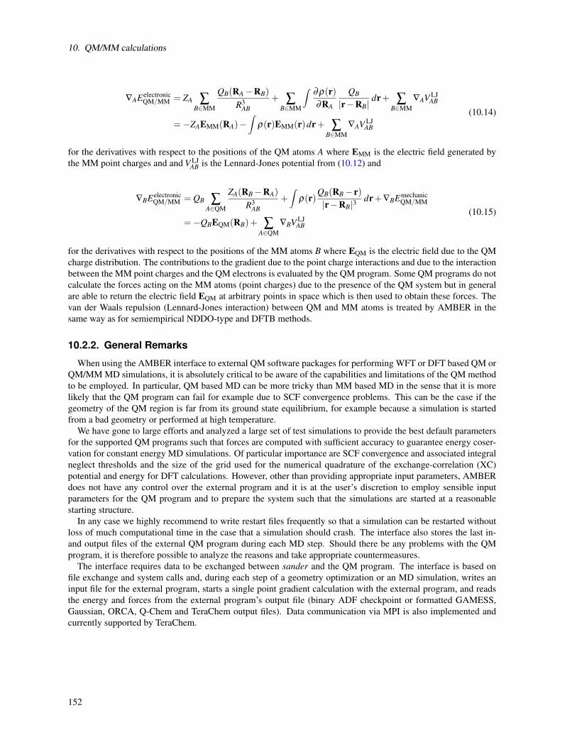
10. QM/MM calculations
∇AEelectronicQM/MM = ZA ∑
B∈MM
QB(RA−RB)
R3AB
+ ∑B∈MM
∫∂ρ(r)∂RA
QB
|r−RB|dr+ ∑
B∈MM∇AV LJ
AB
=−ZAEMM(RA)−∫
ρ(r)EMM(r)dr+ ∑B∈MM
∇AV LJAB
(10.14)
for the derivatives with respect to the positions of the QM atoms A where EMM is the electric field generated bythe MM point charges and and V LJ
AB is the Lennard-Jones potential from (10.12) and
∇BEelectronicQM/MM = QB ∑
A∈QM
ZA(RB−RA)
R3AB
+∫
ρ(r)QB(RB− r)|r−RB|3
dr+∇BEmechanicQM/MM
=−QBEQM(RB)+ ∑A∈QM
∇BV LJAB
(10.15)
for the derivatives with respect to the positions of the MM atoms B where EQM is the electric field due to the QMcharge distribution. The contributions to the gradient due to the point charge interactions and due to the interactionbetween the MM point charges and the QM electrons is evaluated by the QM program. Some QM programs do notcalculate the forces acting on the MM atoms (point charges) due to the presence of the QM system but in generalare able to return the electric field EQM at arbitrary points in space which is then used to obtain these forces. Thevan der Waals repulsion (Lennard-Jones interaction) between QM and MM atoms is treated by AMBER in thesame way as for semiempirical NDDO-type and DFTB methods.
10.2.2. General Remarks
When using the AMBER interface to external QM software packages for performing WFT or DFT based QM orQM/MM MD simulations, it is absolutely critical to be aware of the capabilities and limitations of the QM methodto be employed. In particular, QM based MD can be more tricky than MM based MD in the sense that it is morelikely that the QM program can fail for example due to SCF convergence problems. This can be the case if thegeometry of the QM region is far from its ground state equilibrium, for example because a simulation is startedfrom a bad geometry or performed at high temperature.
We have gone to large efforts and analyzed a large set of test simulations to provide the best default parametersfor the supported QM programs such that forces are computed with sufficient accuracy to guarantee energy coser-vation for constant energy MD simulations. Of particular importance are SCF convergence and associated integralneglect thresholds and the size of the grid used for the numerical quadrature of the exchange-correlation (XC)potential and energy for DFT calculations. However, other than providing appropriate input parameters, AMBERdoes not have any control over the external program and it is at the user’s discretion to employ sensible inputparameters for the QM program and to prepare the system such that the simulations are started at a reasonablestarting structure.
In any case we highly recommend to write restart files frequently so that a simulation can be restarted withoutloss of much computational time in the case that a simulation should crash. The interface also stores the last in-and output files of the external QM program during each MD step. Should there be any problems with the QMprogram, it is therefore possible to analyze the reasons and take appropriate countermeasures.
The interface requires data to be exchanged between sander and the QM program. The interface is based onfile exchange and system calls and, during each step of a geometry optimization or an MD simulation, writes aninput file for the external program, starts a single point gradient calculation with the external program, and readsthe energy and forces from the external program’s output file (binary ADF checkpoint or formatted GAMESS,Gaussian, ORCA, Q-Chem and TeraChem output files). Data communication via MPI is also implemented andcurrently supported by TeraChem.
152

10.2. Interface for ab initio and DFT methods
10.2.3. Limitations
In principle, all types of simulations that are possible with sander are supported. There are, however, somerestrictions for simulations that require sander to run in parallel, in particular path integral molecular dynam-ics (PIMD) and replica exchange molecular dynamics (REMD), see the discussion of Parallelization below. Theinterface to external QM programs also lacks some features regarding solvent models in comparison to the semiem-pirical MNDO and DFTB QM/MM implementation that is available in AMBER, the most critical ones are listedhere.
Generalized Born Generalized Born (GB) implicit solvent models are not supported if external QM programsare used for the QM region.
Particle Mesh Ewald (PME) and Periodic Boundary Conditions The PME approach for treating long-rangeelectrostatic QM/MM and QM/QM interactions in periodic systems is currently not supported. It is possible touse periodic boundary conditions but a cutoff is used for the point charges to be included in the QM Hamiltonian(determined by &qmmm namelist variable qmcut) thus truncating the long-range QM/MM electrostatic interactionsin (10.12). This leads to discontinuities in the potential energy surface and poor energy conservation for MD runsin the NVE ensemble. The user may consider running non-periodic simulations with a cutoff that is larger than thesystem size thus effectively including all interactions.
10.2.4. Performance Considerations
The computational cost of DFT is comparable to Hartree–Fock (HF) theory which is the simplest WFT methodthat serves as zeroth order approximation for more elaborate correlated WFT methods such as Møller–Plesset per-turbation theory, configuration interaction theory and coupled cluster theory. The calculations can be acceleratedby using density fitting approaches, sometimes called resolution-of identity (RI) approximation, which in the caseof DFT with exchange-correlation (XC) functionals that do not require admixture of exact HF-exchange, leads tospeedups of roughly one order of magnitude without compromising the accuracy of the results. Nevertheless, thecomputational cost of DFT is in general two to three orders of magnitude higher than that of semiempirical QMmodels. We recommend to carefully test the performance of the QM program to choose an optimal number ofprocessor counts for parallelized QM calculations. Typical simulation performance for typical QM system sizes oftens of atoms will be on the order of a few picoseconds per day, depending on the underlying QM model chosen.
10.2.5. Parallelization
The MPI parallel executable sander.MPI can be used to run QM/MM MD simulations with external QM softwarein which the MM portion of the calculation is parallelized. However, the computational cost of the MM part isusually small compared to the cost of the QM part. In order to execute the QM part of the calculation in parallel,the external QM program has to be instructed to do so, as described in the sections below.
In the case of PIMD or REMD simulations that require a separate energy and force evaluation for each groupat each time step, the parallelized executable sander.MPI has to be used. Multiple processes can be launched pergroup to parallelize the MM calculations. Care has to be taken to choose the right number of parallel threads inthe external QM program. For example, on a machine with 32 cores, a simulation with 16 beads or replicas canrun the external QM program with 2 threads in parallel to make maximum use of the available processing cores.If the available processors are spread over multiple nodes, special care has to be taken to ensure that the differentinstances of the external QM program are launched on the correct nodes.
It is possible to execute sander.MPI in parallel via MPI while also running MPI or OpenMP parallel versionsof the external QM program. Depending on the MPI implementation, this can, however, fail. In our experience,MPICH and MVAPICH work well while we had problems with OpenMPI.
153
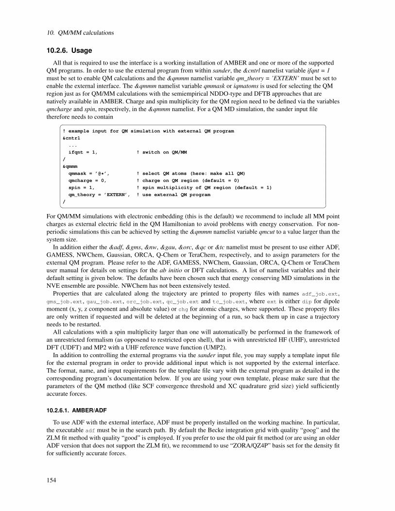
10. QM/MM calculations
10.2.6. Usage
All that is required to use the interface is a working installation of AMBER and one or more of the supportedQM programs. In order to use the external program from within sander, the &cntrl namelist variable ifqnt = 1must be set to enable QM calculations and the &qmmm namelist variable qm_theory = ’EXTERN’ must be set toenable the external interface. The &qmmm namelist variable qmmask or iqmatoms is used for selecting the QMregion just as for QM/MM calculations with the semiempirical NDDO-type and DFTB approaches that arenatively available in AMBER. Charge and spin multiplicity for the QM region need to be defined via the variablesqmcharge and spin, respectively, in the &qmmm namelist. For a QM MD simulation, the sander input filetherefore needs to contain
! example input for QM simulation with external QM program
&cntrl
...
ifqnt = 1, ! switch on QM/MM
/
&qmmm
qmmask = ’@*’, ! select QM atoms (here: make all QM)
qmcharge = 0, ! charge on QM region (default = 0)
spin = 1, ! spin multiplicity of QM region (default = 1)
qm_theory = ’EXTERN’, ! use external QM program
/ For QM/MM simulations with electronic embedding (this is the default) we recommend to include all MM pointcharges as external electric field in the QM Hamiltonian to avoid problems with energy conservation. For non-periodic simulations this can be achieved by setting the &qmmm namelist variable qmcut to a value larger than thesystem size.
In addition either the &adf, &gms, &nw, &gau, &orc, &qc or &tc namelist must be present to use either ADF,GAMESS, NWChem, Gaussian, ORCA, Q-Chem or TeraChem, respectively, and to assign parameters for theexternal QM program. Please refer to the ADF, GAMESS, NWChem, Gaussian, ORCA, Q-Chem or TeraChemuser manual for details on settings for the ab initio or DFT calculations. A list of namelist variables and theirdefault setting is given below. The defaults have been chosen such that energy conserving MD simulations in theNVE ensemble are possible. NWChem has not been extensively tested.
Properties that are calculated along the trajectory are printed to property files with names adf_job.ext,gms_job.ext, gau_job.ext, orc_job.ext, qc_job.ext and tc_job.ext, where ext is either dip for dipolemoment (x, y, z component and absolute value) or chg for atomic charges, where supported. These property filesare only written if requested and will be deleted at the beginning of a run, so back them up in case a trajectoryneeds to be restarted.
All calculations with a spin multiplicity larger than one will automatically be performed in the framework ofan unrestricted formalism (as opposend to restricted open shell), that is with unrestricted HF (UHF), unrestrictedDFT (UDFT) and MP2 with a UHF reference wave function (UMP2).
In addition to controlling the external programs via the sander input file, you may supply a template input filefor the external program in order to provide additional input which is not supported by the external interface.The format, name, and input requirements for the template file vary with the external program as detailed in thecorresponding program’s documentation below. If you are using your own template, please make sure that theparameters of the QM method (like SCF convergence threshold and XC quadrature grid size) yield sufficientlyaccurate forces.
10.2.6.1. AMBER/ADF
To use ADF with the external interface, ADF must be properly installed on the working machine. In particular,the executable adf must be in the search path. By default the Becke integration grid with quality “goog” and theZLM fit method with quality “good” is employed. If you prefer to use the old pair fit method (or are using an olderADF version that does not support the ZLM fit), we recommend to use “ZORA/QZ4P” basis set for the density fitfor sufficiently accurate forces.
154

10.2. Interface for ab initio and DFT methods
Limitations At present only mechanical embedding is supported.
&adf Namelist variables
basis Basis set type to be used in the DFT calculation. Valid standard basis set types are: SZ, DZ, DZP,TZP, TZ2P, TZ2P+ and ZORA/QZ4P. (Default: basis = ’DZP’)
core Type of frozen core to use. Allowed values are: None, Small, Medium, Large. (Default: core =’None’)
zlmfit Quality of density fit with the ZLM fit method. (Default: zlmfit = ’good’)
fit_type Fit basis set type to be used for density fitting with the old pair fit method. Valid values are identicalto the available basis sets (SZ, DZ etc) in which case the fit basis corresponding to the AO Basis willbe used. By default the ZLM fit method will be used (Default: fit_type = ”)
xc Exchange-correlation functional to be used. Popular choices are ’LDA VWN’, ’GGA BLYP’, ’GGAPBE’, ’HYBRID B3LYP’ and ’HYBRID PBE0’. Consult the ADF manual for all available options.(Default: xc = ’GGA BLYP’)
scf_iter Maximum number of SCF cycles allowed. (Default: scf_iter = 50)
scf_conv Threshold upon which to stop the SCF procedure. The tested error is the commutator of the Fockmatrix and the density matrix. Convergence is considered to be achieved if the maximum element ofthe commutator (which is zero for an optimized wave function) is smaller than scf_conv. (Default:scf_conv = 1.0d-06)
beckegrid Quality of Becke integration grid. Allowed values are: Normal, Good, VeryGood. (Default: core =’Good’)
integration Numerical integration accuracy for integration with olde teVelde-Baerends integration grid (Voronoicells). By default the Becke grid will be used. The old integration grid can be used by specifying anumber larger than 0, we recommend at least 5.0. (Default: integration = -1.0)
num_threads Number of threads (and thus CPU cores) for ADF to use. Note that this is not requied if you arerunning in a queuing system as ADF will automatically use the full number of reserved cores. (Default:num_threads = 0 [this causes ADF to use all available cores on a machine])
use_dftb Specifies whether DFTB shall be used with ADF’s DFTB program dftb. If use_dftb = 1 then DFTBwill be used and only variables charge and scf_conv will be considered. (Default: use_dftb = 0 [donot use DFTB, regular DFT calculation]) - works only with older DFTB versions (prior to 2011).
exactdensity The exact (as opposed to fitted) electron density is used for the evaluation of the exchange-correlationpotential if exactdensity = 1. (Default: exactdensity = 0)
use_template Determine whether or not to use a user-provided template file for running external programs. (De-fault: use_template = 0)
ntpr Controls frequency of printing for dipole moment to file adf_job.dip (Defaults to &cntrl namelistvariable ntpr)
dipole Toggles writing of dipole moment to file adf_job.dip (Default: dipole = 0)
155
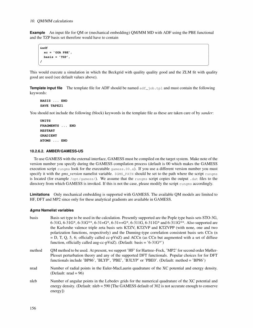
10. QM/MM calculations
Example An input file for QM or (mechanical embedding) QM/MM MD with ADF using the PBE functionaland the TZP basis set therefore would have to contain
&adf
xc = ’GGA PBE’,
basis = ’TZP’,
/ This would execute a simulation in which the Beckgrid with quality quality good and the ZLM fit with qualitygood are used (see default values above).
Template input file The template file for ADF should be named adf_job.tpl and must contain the followingkeywords:
BASIS ... END
SAVE TAPE21
You should not include the following (block) keywords in the template file as these are taken care of by sander:
UNITS
FRAGMENTS ... END
RESTART
GRADIENT
ATOMS ... END
10.2.6.2. AMBER/GAMESS-US
To use GAMESS with the external interface, GAMESS must be compiled on the target system. Make note of theversion number you specify during the GAMESS compilation process (default is 00 which makes the GAMESSexecution script rungms look for the executable gamess.00.x). If you use a different version number you mustspecify it with the gms_version namelist variable. $GMS_PATH should be set to the path where the script rungmsis located (for example /opt/gamess/). We assume that the rungms script copies the output .dat files to thedirectory from which GAMESS is invoked. If this is not the case, please modify the script rungms accordingly.
Limitations Only mechanical embedding is supported with GAMESS. The available QM models are limited toHF, DFT and MP2 since only for these analytical gradients are available in GAMESS.
&gms Namelist variables
basis Basis set type to be used in the calculation. Presently supported are the Pople type basis sets STO-3G,6-31G, 6-31G*, 6-31G**, 6-31+G*, 6-31++G*, 6-311G, 6-311G* and 6-311G**. Also supported arethe Karlsruhe valence triple zeta basis sets KTZV, KTZVP and KTZVPP (with none, one and twopolarization functions, respectively) and the Dunning-type correlation consistent basis sets CCn (n= D, T, Q, 5, 6; officially called cc-pVnZ) and ACCn (as CCn but augmented with a set of diffusefunction, officially called aug-cc-pVnZ). (Default: basis = ’6-31G*’)
method QM method to be used. At present, we support ’HF’ for Hartree–Fock, ’MP2’ for second order Møller-Plesset perturbation theory and any of the supported DFT functionals. Popular choices for for DFTfunctionals include ’BP86’, ’BLYP’, ’PBE’, ’B3LYP’ or ’PBE0’. (Default: method = ’BP86’)
nrad Number of radial points in the Euler-MacLaurin quadrature of the XC potential and energy density.(Default: nrad = 96)
nleb Number of angular points in the Lebedev grids for the numerical quadrature of the XC potential andenergy density. (Default: nleb = 590 [The GAMESS default of 302 is not accurate enough to conserveenergy])
156

10.2. Interface for ab initio and DFT methods
scf_conv SCF convergence threshold. Convergence is reached when the absolute density change between twoconsecutive SCF cycles is less than scf_conv. (Default: scf_conv = 1.0D-06)
maxit Maximum number of SCF iterations. (Default: maxit = 50)
gms_version This is the version number specified when building GAMESS. (Default: gms_version = 00)
num_threads Number of threads (and thus CPU cores) for GAMESS to use. Note that GAMESS may require aspecial setup in the rungms script to be able to run using multiple threads. Unless num_threads isexplicitly specified, GAMESS will only use one thread (run on one core). (Default: num_threads = 1)
mwords The maximum replicated memory which your job can use, on every node. This is given in units of1,000,000 words (as opposed to 1024*1024 words), where a word is defined as 64 bits. You mayneed to increase this value if GAMESS crashes due to not having enough memory allocated. (Default:mwords = 50)
use_template Determine whether or not to use a user-provided template file for running external programs. (De-fault: use_template = 0)
ntpr Controls frequency of printing for dipole moment and atomic charges to files gms_prop.ext (Defaultsto &cntrl namelist variable ntpr)
chelpg CHELPG charges are calculated if chelpg = 1. These charges are written to the file gms_prop.chg
(Default: chelpg = 0)
dipole Toggles writing of dipole moment to file gms_prop.dip (Default: dipole = 0)
Example An input file for QM or (mechanical embedding) QM/MM MD with GAMESS using the PBEfunctional and the 6-31G** basis set that should run GAMESS on 16 CPU cores therefore would have to contain
&gms
method = ’DFT’,
dfttyp = ’PBE’,
basis = ’6-31G**’,
num_threads = 16,
/ Template input file The template file for GAMESS should be named gms_job.tpl and the $CONTRL card mustcontain the following keywords:
RUNTYP=GRADIENT
UNIT=ANGS
COORD=UNIQUE
You should not include the $DATA card in the template file as it is taken care of by sander.
10.2.6.3. AMBER/Gaussian
To use Gaussian with the interface, Gaussian03 or Gaussian09 must be properly installed on the system and theg03 or g09 executable must be in the path.
Limitations A cutoff is applied to QM/MM interactions in QM/MM simulations using electrostatic embeddingwith and without PBCs. This leads to discontinuities in the potential energy surface and poor energy conservation.In the case of QM/MM simulations without PBCs, this cutoff (qmcut variable in the &qmmm namelist) can be setto a number that is larger than the simulated system, thus effectively not applying a cutoff. This is recommended.
157

10. QM/MM calculations
&gau Namelist variables
basis Basis set type to be used in the calculation. Any basis set that is natively supported by Gaussian canbe used. Examples are the single zeta, split valence or triple zeta Pople type basis sets ’STO-3G’, ’3-21G’, ’6-31G’ and ’6-311G’. The split-valence or triple zeta basis sets can be augmented with diffusefunctions on heavy atoms or additionally hydrogen by adding one or two plus signs, respectively, as in’6-31++G’. Polarization functions on heavy atoms or additionally hydrogens are used by adding oneor two stars, respectively, as in ’6-31G**’. (Default: basis = ’6-31G*’)
method Method to be used in the calculation. Can either be one of the WFT models for which Gaussiansupports gradients, for example ’RHF’ or ’MP2’, or some supported DFT functional. Popular choicesare ’BLYP’, ’PBE’ and ’B3LYP’. (Default: method = ’BLYP’)
scf_conv Threshold upon which to stop the SCF procedure. The tested error is the commutator of the Fockmatrix and the density matrix. Convergence is considered to be achieved if the maximum element ofthe commutator (which is zero for an optimized wave function) is smaller than scf_conv. Set in theform of 10−N . (Default: scf_conv = 8)
num_threads Number of threads (and thus CPU cores) for Gaussian to use. Unless num_threads is explicitlyspecified, Gaussian will only use one thread (run on one core). (Default: num_threads = 1)
use_template Determine whether or not to use a user-provided template file for running external programs. (De-fault: use_template = 0)
ntpr Controls frequency of printing for dipole moment to file gau_job.dip (Defaults to &cntrl namelistvariable ntpr)
dipole Toggles writing of dipole moment to file gau_job.dip (Default: dipole = 0)
mem String that specifies how much memory Gaussian should be allowed to use. (Default: ’256MB’)
Example An input file for QM or QM/MM MD with Gaussian using the BP86 functional and the 6-31G**basis set and running in parallel on 8 threads (using 1 GB of memory) therefore would have to contain
&gau
method = ’BP86’,
basis = ’6-31G**’,
num_threads = 8,
mem=’1GB’,
/ Template input file The template file for Gaussian should be named gau_job.tpl and should only contain theroute section of a Gaussian input file. The route section defines the method to be used and SCF convergencecriteria. Charge and spin multiplicity are provided by via the &qmmm namelist. For example for a B3LYPcalculation with 6-31G* basis set, the route section would be:
#P B3LYP/6-31G* SCF=(Conver=8)
Do not include any information about coordinates or point charge treatment since this will all be handled by sander.Also, do not include any Link 0 Commands (line starting with %) since these are handled by sander. If you wantto run Gaussian in parallel, specify the number of processors via the num_threads variable in the &gau namelist.
10.2.6.4. AMBER/Orca
To use Orca with the interface, Orca must be properly installed on the system, the Orca executables need toreside in a directory that is in the search path. For convenience of use, namelist parameters in general correspondto Orca keywords, see the Orca manual for details.
158

10.2. Interface for ab initio and DFT methods
Limitations A cutoff is applied to QM/MM interactions in QM/MM simulations with and without PBCs. Thisleads to discontinuities in the potential energy surface and poor energy conservation. In the case of QM/MMsimulations without PBCs, this cutoff (qmcut variable in the qmmm namelist) can be set to a number that is largerthan the simulated system, thus effectively not applying a cutoff. This is recommended.
Also note that ORCA only supports OpenMPI for parallel calculations.
&orc Namelist variables
basis Basis set type to be used in the calculation. Possible choices include ’svp’, ’6-31g’, etc. See Orcamanual for a complete list. (Default: basis = ’SV(P)’)
cbasis Auxillary basis set for correlation fitting. See Orca manual for a complete list. (Default: basis =’NONE’)
jbasis Auxillary basis set for Coulomb fitting. See Orca manual for a complete list. (Default: basis =’NONE’)
method Method to be used in the calculation. Popular choices include ’hf’, ’pm3’, ’blyp’, and ’mp2’. (Default:method = ’blyp’)
convkey General SCF convergence setting for simplified Orca input. Can take values ’TIGHTSCF’, ’VERY-TIGHTSCF’, etc. (Default: convkey=’VERYTIGHTSCF’)
scfconv SCF convergence threshold for the energy. (Default: scfconv = -1, that is, not in use since we use thegeneral convergence settings keyword convkey. Otherwise this would lead to SCF energy convergenceof 10−Nau, if set to N.)
grid Grid type used during the SCF for the XC quadrature in DFT. (Default: grid = 4, this corresponds toIntacc = 4.34 for the radial grid and an angular Lebedev grid with 302 points. Conservatively chosentogether with finalgrid to conserve energy.)
finalgrid Grid type used for the energy and gradient calculation after the SCF for the XC quadrature in DFT.(Default: finalgrid = 6, this corresponds to Intacc = 5.34 for the radial grid and an angular Lebedevgrid with 590 points. Conservatively chosen together with grid to conserve energy.)
maxiter Maximum number of SCF iteractions. (Default maxiter = 100)
maxcore Global scratch memory (in MB) used by Orca. You may need to increase this when running largerjobs. See Orca manual for more information. (Default maxcore = 1024)
num_threads Number of threads (and thus CPU cores) for Orca to use. Note that Orca only supports OpenMPI.(Default: num_threads = 1)
use_template Determine whether or not to use a user-provided template file for running external programs. (De-fault: use_template = 0)
ntpr Controls frequency of printing for the dipole moment to file orc_job.dip (Defaults to &cntrl namelistvariable ntpr)
dipole Toggles writing of the dipole moment to file orc_job.dip (Default: dipole = 0)
Example An input file for QM or QM/MM MD with Orca using the BLYP functional, the SVP basis settherefore would have to contain
&orc
method = ’blyp’,
basis = ’svp’,
/ 159
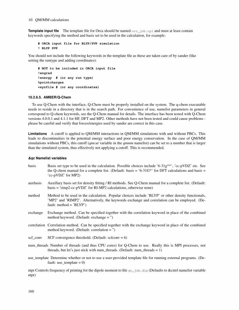
10. QM/MM calculations
Template input file The template file for Orca should be named orc_job.tpl and must at least containkeywords specifying the method and basis set to be used in the calculation, for example:
# ORCA input file for BLYP/SVP simulation
! BLYP SVP
You should not include the following keywords in the template file as these are taken care of by sander (likesetting the runtype and adding coordinates):
# NOT to be included in ORCA input file
!engrad
!energy # (or any run type)
%pointcharges
*xyzfile # (or any coordinates)
10.2.6.5. AMBER/Q-Chem
To use Q-Chem with the interface, Q-Chem must be properly installed on the system. The q-chem executableneeds to reside in a directory that is in the search path. For convenience of use, namelist parameters in generalcorrespond to Q-chem keywords, see the Q-Chem manual for details. The interface has been tested with Q-Chemversions 4.0.0.1 and 4.1.1 for HF, DFT and MP2. Other methods have not been tested and could cause problems -please be careful and verify that forces/energies used by sander are correct in this case.
Limitations A cutoff is applied to QM/MM interactions in QM/MM simulations with and without PBCs. Thisleads to discontinuities in the potential energy surface and poor energy conservation. In the case of QM/MMsimulations without PBCs, this cutoff (qmcut variable in the qmmm namelist) can be set to a number that is largerthan the simulated system, thus effectively not applying a cutoff. This is recommended.
&qc Namelist variables
basis Basis set type to be used in the calculation. Possible choices include ’6-31g**’, ’cc-pVDZ’ etc. Seethe Q-chem manual for a complete list. (Default: basis = ’6-31G*’ for DFT calculations and basis =’cc-pVDZ’ for MP2)
auxbasis Auxillary basis set for density fitting / RI methods. See Q-Chem manual for a complete list. (Default:basis = ’rimp2-cc-pVDZ’ for RI-MP2 calculations, otherwise none)
method Method to be used in the calculation. Popular choices include ’BLYP’ or other density functionals,’MP2’ and ’RIMP2’. Alternatively, the keywords exchange and correlation can be employed. (De-fault: method = ’BLYP’)
exchange Exchange method. Can be specified together with the correlation keyword in place of the combinedmethod keyword. (Default: exchange = ”)
correlation Correlation method. Can be specified together with the exchange keyword in place of the combinedmethod keyword. (Default: correlation = ”)
scf_conv SCF convergence threshold. (Default: scfconv = 6)
num_threads Number of threads (and thus CPU cores) for Q-Chem to use. Really this is MPI processes, notthreads, but let’s just stick with num_threads. (Default: num_threads = 1)
use_template Determine whether or not to use a user-provided template file for running external programs. (De-fault: use_template = 0)
ntpr Controls frequency of printing for the dipole moment to file qc_job.dip (Defaults to &cntrl namelist variablentpr)
160

10.2. Interface for ab initio and DFT methods
dipole Toggles writing of the dipole moment to file qc_job.dip. This is currently not supported. (Default:dipole = 0)
guess Toggles use of MOs from previous step as initial guess to accelerate SCF convergence. Any stringdifferent from ’read’ will disable this. (Default: guess = ’read’)
Example An input file for QM or QM/MM MD with Q-Chem using MP2 with the cc-pVTZ basis set thereforewould have to contain
&qc
method = ’mp2’,
basis = ’cc-pVTZ’,
/ Template input file The template file for Q-chem must be named qc_job.tpl and must only contain keywordsin the Q-Chem $rem input section that specify the QM method and basis set to be used in the calculation, forexample:
EXCHANGE becke
CORRELATION lyp
BASIS 6-311G**SCF_CONVERGENCE 7
The interface will take care of adding other keywords to the $rem section such as JOBTYPE and writing the$molecule input file sections.
10.2.6.6. AMBER/TeraChem
To use TeraChem with the interface, TeraChem must be properly installed on the system. In particular, theterachem executable needs to be in the search path. Namelist parameters correspond to TeraChem keywords, seethe TeraChem manual for details.
Limitations A cutoff is applied to QM/MM interactions in QM/MM simulations with and without PBCs. Thisleads to discontinuities in the potential energy surface and poor energy conservation. In the case of QM/MMsimulations without PBCs, this cutoff (qmcut variable in the &qmmm namelist) can be set to a number that islarger than the simulated system, thus effectively not applying a cutoff. This is recommended.
&tc Namelist variables
basis Basis set type to be used in the calculation. Possible choices presently (TeraChem version 1.4) are’STO-3G’, ’3-21G’, ’6-31G’ and ’6-311G’, ’3-21++G’ and ’6-31++G’ (Default: basis = ’6-31G’)
method Method to be used in the calculation, can be either ’RHF’ or some supported DFT functional. Popularchoices are ’BLYP’, ’PBE’ and ’B3LYP’. (Default: method = ’BLYP’)
dftd Determines whether dispersion corrections are applied in the case of DFT calculations. (Default: dftd= ’no’)
precision Precision model setting (single vs double precision). (Default: precision = ’mixed’)
dynamicgrid Use coarse grid during early SCF iterations. (Default: dynamicgrid = ’yes’)
threall Determines a variety of thresholds. (Default: threall = 1.0E-11)
convthre SCF convergence threshold for the wavefunction. (Default: convthre = 3.0E-05, which leads to SCFenergy convergence of approximately 10−7 au or 10−4 kcal/mol)
161

10. QM/MM calculations
maxit Maximum number of SCF iterations. (Default: maxit = 100)
dftgrid DFT grid to be employed for the numerical XC quadrature in DFT calculations. (Default: dftgrid = 1)
ngpus Determines how many GPUs are to be used. (Default: ngpus = 0, which uses all available GPUs)
gpuids If ngpus has a value other than zero, this determines the IDs of the GPUs to be used for the calculation.(Default: gpuids = 0, 1, 2, etc.)
executable Name of the TeraChem executable. (Default: executable = terachem)
use_template Determine whether or not to use a user-provided template file for running external programs. (De-fault: use_template = 0)
ntpr Controls frequency of printing for dipole moment and atomic charges to files tc_job.ext. (Defaultsto &cntrl namelist variable ntpr)
charge_analysis Toggles writing of atomic charges to file tc_job.chg (Options: ’none’ or ’Mulliken’. Default:dipole = ’none’)
dipole Toggles writing of dipole moment to file tc_job.dip (Default: dipole = 0)
Example An input file for QM or QM/MM MD with TeraChem using the PBE functional and the 6-31G* basisset therefore would have to contain
&tc
method = ’PBE’,
basis = ’6-31G*’,
/ Template input file The template file for Terachem should be named tc_job.tpl and must at least contain thefollowing keywords:
basis
method
Any content of the template file after a line containing the end keyword will be ignored.You should not include the following keywords in the template file as these are taken care of by sander.
Instead, specify these via the &qmmm or &tc namelist:
run
charge
spinmult
coordinates
pointcharges
amber
gpus
10.3. Adaptive solvent QM/MM simulations
Traditional QM/MM approaches are based on a static QM/MM partitioning in which atoms belonging to theQM and MM regions are selected at the beginning of a molecular dynamics simulation. Such a static partitioningcannot be applied if part of the bulk solvent in the vicinity of a region of interest needs to be included in the QMregion. Examples include cases in which the bulk solvent participates directly in a chemical reaction or in whichimportant interactions between the solute and the bulk solvent, such as polarization and charge transfer, are not
162

10.3. Adaptive solvent QM/MM simulations
well parameterized at the QM/MM level and thus need to be described quantum mechanically. Due to moleculardiffusion, solvent molecules will constantly exchange between the QM and MM regions and thus require a specialtreatment.
Several approaches have been developed that allow molecules to change their QM or MM character when cross-ing the boundaries between the QM and MM regions. A good overview and comparison of these approachesis available in the work by Bulo et al.[292]. One of the most accurate approaches is the difference-based adap-tive solvation (DAS) method[293], in the following simply called adaptive QM/MM (adQM/MM). This methodis available in Amber through a parallelized implementation that has been developed by Andreas Goetz (SDSC)with help from Ross Walker (SDSC), Rosa Bulo (Utrecht University) and Kyoyeon Park (UCSD). The useful-ness of this adQM/MM approach for aqueous systems has been demonstrated with a development version of thisimplementation[294]. If you publish work that results from using this implementation, please cite the followingwork:
• A. W. Götz, K. Park, R. E. Bulo, F. Paesani, R. C. Walker, Efficient adaptive QM/MM implementation:Application to ion binding by peptides in solution, in preparation.
• R. E. Bulo, B. Ensing, J. Sikkema, L. Visscher, Toward a practical method for adaptive QM/MM simulations,J. Chem. Theory Comput. 9, 2212-2221 (2009), DOI: 10.1021/ct900148e
In what follows we will describe the theoretical background of this implementation and how to perform adQM/MMsimulations. For an alternative approach, see section 10.4.
10.3.1. Theoretical background
In adQM/MM simulations, we distinguish three different regions, an active region (A), a transition region (T),and the environment region (E). The active region contains both the part of the system that is permanently treatedquantum mechanically (similar to the QM region in regular QM/MM simulations) and the solvent molecules in itsvicinity that are also treated quantum mechanically. The E region is the part of the system that is treated at the MMlevel. Within the T region, molecules change their character from purely QM to purely MM, that is, molecules inthe T region have partial QM and MM character, depending on their position within the T region. The T region thatconnects the A and E regions is required to guarantee that the potential energy surface or forces remain continuousthroughout the simulation.
10.3.1.1. System partitioning
In the adQM/MM method[293], a partial MM character λ is assigned to each molecule in the T region. Thevalue of λ depends on the distance of the molecule from the center of the A region according to
λ (r) =
0 r ≤ RA(r−RA)
2(3RT−RA−2r)(RT−RA)3 RA < r < RT
1 r ≥ RT
, (10.16)
where RA and RT are the inner and outer radii delimiting the T region. The switching function thus interpolatessmoothly between QM (A region) and MM (E region).
The adQM/MM energy can be constructed as a weighted average of regular QM/MM energies due to all possible2NT partitionings in which the NT molecules in the T region are assigned either to the QM or the MM region,
EadQM/MM = ∑a
σaEQM/MMa . (10.17)
The statistical coefficients σa for the QM/MM partitionings are defined on basis of the λ values defined above,
σa =
0 ifmax(λQM
a )> min(λMMa )
min(λMMa )−max(λQM
a ) ifmax(λQMa )≤min(λMM
a ), (10.18)
163

10. QM/MM calculations
where λQMa and λMM
a are the sets of λ values for a given QM/MM partitioning a that are assigned to the QMand MM regions, respectively. Due to this choice of coefficients, the weight σa of a QM/MM partitioning is zero ifthe partition contains one or more MM molecules closer to the A region than any of the QM molecules. The totalnumber of nonzero QM/MM partitionings in an adQM/MM simulations is thus NT +1. In addition it is guaranteedthat the weight of each partition varies smoothly from 0 to 1, removing discontinuities in the system dynamics thatwould appear in standard QM/MM simulations if a molecule would change its character by diffusing in or out ofthe QM region.
10.3.1.2. Force interpolation
The forces resulting from the adQM/MM energy 10.17 are a weighted sum of the force from each nonzeroQM/MM partitioning and also contain a term that depends on the derivatives of the weight functions,
FadQM/MM =−∑a
[σa
∂EQM/MMa
∂R+
∂σa
∂REQM/MM
a
]. (10.19)
This introduces an artificial dependence on the relative energies of the different QM/MM partitionings. Thus, inplace of the energy interpolation scheme, a force interpolation is applied in which the forces are given as
FadQM/MM =−∑a
σa∂EQM/MM
a
∂R. (10.20)
The force interpolation does not conserve the energy from equation 10.17 but it is possible to define a conservedquantity according to
EadQM/MM = EadQM/MM +W, (10.21)
where the correction term W is defined through
∂W∂R
=−∑a
∂σa
∂REQM/MM
a . (10.22)
The quantity EadQM/MM is not a potential energy since it is only defined along the path taken by the system duringthe simulation. It is nevertheless useful to monitor this quantity to determine whether the simulation settings leadto numerical stability. The correction term W can be expressed as the path integral of its force vector from equation10.22, which can be discretized. For step n of an MD simulation it is given as
Wn =n
∑i
∑a
EQM/MMa (i)
σa(i+1)−σa(i−1)2
. (10.23)
The Amber implementation uses exclusively the force interpolation scheme from equation 10.20 and optionallycomputes the correction term W from equation 10.23 to enable monitoring of the conserved quantity EadQM/MM
from equation 10.21.
10.3.1.3. Alternative definitions of active, transition and environment regions
So far we have defined the boundaries between the A, T, and E regions with the distances RA and RT fromthe center of the active region. In this case both the A and the T regions have fixed volumes but the numberof solvent molecules inside each region can vary during the simulation. Alternatively, we can fix the number ofsolvent molecules NA and NT within the A and T regions, respectively. In this case the volume of the A andT regions as well as the radii RA and RT will vary during the course of a simulation. The advantage of fixingthe number of solvent molecules in the T region is that the number of QM/MM partitionings that needs to beconsidered also remains constant (NT + 1). This is useful to optimize load balancing in a parallel adQM/MMimplementation. The downside is that expression 10.23 does not strictly hold any more since the coefficients σadepend on the λ values which in turn depend on RA and RT. However, in practice, this is usually not an issue since
164

10.3. Adaptive solvent QM/MM simulations
the conserved quantity EadQM/MM needs monitoring only during simulation setup to choose settings that affordsufficient numerical stability. One thus can test simulation settings with fixed radii RA and RT and then switch tofixed molecule numbers NA and NT for production runs.
10.3.2. Running adQM/MM simulations with sander
Performing simulations with the adQM/MM approach described above requires the MPI parallelized sanderexecutable sander.MPI. The implementation features a dual layer parallelization in which the calculations for allindividual QM/MM partitionings are performed in parallel. Each of these QM/MM calculations can in turn be runin parallel. The parallelization across QM/MM partitionings is based on the multisander code infrastructure whicheffectively runs independent copies of sander for each QM/MM partitioning (similar to the replica exchange, pathintegral and thermodynamic integration implementations).
In order to run an adQM/MM simulation, the mdin input file needs to be set up similar to a regular QM/MMsimulation. The QM region as defined in the &qmmm namelist defines the atoms that are in the permanent QMregion. In addition, the &qmmm namelist variable vsolv needs to be set to 2 or 3 for fixed number of moleculesin the A and T region or fixed size of A and T region, respectively. The following shows the minimum additionsto the mdin input file that are required to perform an adQM/MM simulation as compared to a traditional QM/MMsimulation with fixed QM and MM regions: # mdin file - minimum additional content for adaptive solvent QM/MM
&qmmm
...
adjust_q = 0, ! required, charge cannot be redistributed
vsolv = 2, ! switch on adQM/MM with fixed molecule numbers
! in A and T region
/
&vsolv
nearest_qm_solvent = 6, ! number of solvent molecules in A region
/
&adqmmm
n_partition = 4, ! number of QM/MM partitionings
! = number of molecules in T region + 1
/ In this example, a fixed number of solvent molecules is contained in the A region (6) and in the T region (3, sincethe number of QM/MM partitionings is NT + 1). Thus, the volume of the A and T regions changes during thesimulation. Details of all namelist variables are collected below.
In addition, a groupfile for multisander is required. This groupfile should point all sander copies to the samemdin input file, inpcrd coordinate file and prmtop parameter and topology file: # groupfile for adaptive solvent QM/MM run with n_partition = 4
-O -i mdin -c inpcrd -p prmtop
-O -i mdin -c inpcrd -p prmtop
-O -i mdin -c inpcrd -p prmtop
-O -i mdin -c inpcrd -p prmtop If you explicitly specify output file names, make sure to give separate names to each group (for examplemdout.000, mdout.001 etc), see also the multisander documentation. The mutisander adQM/MM simulationcan then be executed with mpirun -np 4 sander.MPI -rem 0 -ng 4 -groupfile groupfile In this example, 4 MPI processes will be launched for 4 process groups (sander copies). The individual QM/MMcalculations for each partitioning would thus run in serial. To run the individual QM/MM calculations in parallel,the number of MPI processes must be a multiple of the number of process groups.
165

10. QM/MM calculations
Adaptive solvent QM/MM simulations can be performed both with the semiempirical NDDO-type and DFTBmethods that are native to sander or with QM methods that are available via the interface to external QM pro-grams. In the latter case, each process group will launch only one instance of the external QM program andthe parallelization of the QM part of the QM/MM calculations is determined by the settings for the external QMprogram.
10.3.2.1. Important notes for system preparation and adQM/MM simulations
At the time of writing (release of AMBER 16) there is only a limited body of experience with adQM/MMsimulations documented in the literature. Running adQM/MM simulations requires careful simulation setup, inparticular regarding the size of the A and T regions. The A region needs to be sufficiently large to correctly describethe physics of the system of interest. The T region on the other hand needs to be sufficiently large to minimize forceinterpolation errors between the QM and MM regions. Since the cost of an adQM/MM simulation scales linearlywith the number of molecules in the T region, a tradeoff between accuracy and cost often needs to be made. Thisin turn might lead to simulations that behave nicely for many time steps but eventually experience sudden, large(unphysical) forces on atoms at the T region boundaries. Similarly, whether it is more appropriate to define thecenter of the A region via an atom or the center of mass of the permanent QM region will affect the numericalstability of a simulation, depending on the particular system. Likewise for determining the distances of the solventmolecules via an atom or the center of mass of the solvent. In the case of water as solvent, problems can arise dueto autoprotolysis which can lead to the formation of hydroxide and hydronium ions in the A region. Since the MMforce field is not parameterized for hydroxide or hydronium ions, these will experience strong (unphysical) forcesupon entering the T region. Careful monitoring of adQM/MM simulations and a bit of patience is thus advisable.It is a good idea to monitor the size of the A and T region and to check coordinates of atoms in the QM regions ofall partitionings.
10.3.2.2. Namelist parameters for adaptive solvent QM/MM simulations
Adaptive solvent QM/MM simulations require setting the vsolv variable in the &qmmm namelist and settingvariables in the &vsolv and &adqmmm namelists.
&vsolv namelist parameters The &vsolv namelist contains parameters that describe which solvent moleculesare contained in the A region in addition to the permanent QM region that is defined in the &qmmm namelist. Thisnamelist can be used without the &adqmmm namelist in a regular QM/MM simulation with sander if the variablevsolv in the &qmmm namelist is set to 1 instead of 2 or 3 (see 10.1.6). In this case there is no transition region andsolvent molecules entering / leaving the QM region during the simulation would switch abruptly between QM andMM description. This is not recommended since it will results in large unphysical forces whenever such a switchoccurs. However, this option is useful for post-processing of trajectories with single point QM/MM calculations inwhich the solvent molecules closest to the permanent QM region are treated quantum mechanically.
nearest_qm_solvent_resname Residue name of the solvent that can exchange between QM and MM region (De-fault: nearest_qm_solvent_resname = ’WAT’)
nearest_qm_solvent Number of solvent molecules in the A region (Default: nearest_qm_solvent = 0)
nearest_qm_solvent_fq Frequency of updating of the A region. Should be set to 1 (every MD step) for adQM/MMsimulations. (Default: nearest_qm_solvent_fq = 1)
nearest_qm_solvent_center_id Determines the atom(s) of the solvent molecules that is used to calculate the dis-tance to the QM region.
= 0 Use the atom that is closest to the QM region. (default)
= -1 Use the center of mass.
> 0 Use this atom number within the solvent residue.
166
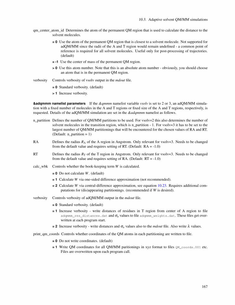
10.3. Adaptive solvent QM/MM simulations
qm_center_atom_id Determines the atom of the permanent QM region that is used to calculate the distance to thesolvent molecules.
= 0 Use the atom of the permanent QM region that is closest to a solvent molecule. Not supported foradQM/MM since the radii of the A and T region would remain undefined - a common point ofreference is required for all solvent molecules. Useful only for post-processing of trajectories.(default)
= -1 Use the center of mass of the permanent QM region.
> 0 Use this atom number. Note that this is an absolute atom number - obviously, you should choosean atom that is in the permanent QM region.
verbosity Controls verbosity of vsolv output in the mdout file.
= 0 Standard verbosity. (default)
> 1 Increase verbosity.
&adqmmm namelist parameters If the &qmmm namelist variable vsolv is set to 2 or 3, an adQM/MM simula-tion with a fixed number of molecules in the A and T regions or fixed size of the A and T regions, respectively, isrequested. Details of the adQM/MM simulation are set in the &adqmmm namelist as follows.
n_partition Defines the number of QM/MM partitions to be used. For vsolv=2 this also determines the number ofsolvent molecules in the transition region, which is n_partition - 1. For vsolv=3 it has to be set to thelargest number of QM/MM partitionings that will be encountered for the chosen values of RA and RT.(Default: n_partition = 1)
RA Defines the radius RA of the A region in Angstrom. Only relevant for vsolv=3. Needs to be changedfrom the default value and requires setting of RT. (Default: RA = -1.0)
RT Defines the radius RT of the T region in Angstrom. Only relevant for vsolv=3. Needs to be changedfrom the default value and requires setting of RA. (Default: RT = -1.0)
calc_wbk Controls whether the book-keeping term W is calculated.
= 0 Do not calculate W . (default)
= 1 Calculate W via one-sided difference approximation (not recommended).
= 2 Calculate W via central-difference approximation, see equation 10.23. Requires additional com-putations for (dis)appearing partitionings. (recommended if W is desired).
verbosity Controls verbosity of adQM/MM output in the mdout file.
= 0 Standard verbosity. (default)
= 1 Increase verbosity - write distances of residues in T region from center of A region to fileadqmmm_res_distances.dat and σa values to file adqmmm_weights.dat. These files get over-written at each program start.
= 2 Increase verbosity - write distances and σa values also to the mdout file. Also write λ values.
print_qm_coords Controls whether coordinates of the QM atoms in each partitioning are written to file.
= 0 Do not write coordinates. (default)
= 1 Write QM coordinates for all QM/MM paritionings in xyz format to files QM_coords.001 etc.Files are overwritten upon each program call.
167

10. QM/MM calculations
10.4. Adaptive buffered force-mixing QM/MM
10.4.1. Introduction
In hybrid quantum mechanical – molecular mechanical (QM/MM) methods the reactive part of the system (i.e.where a significant change of the charge density distribution is expected) is described using a quantum mechanicalmodel while the rest of the system is treated using molecular mechanics. Conventional (“energy-mixing”) QM/MMmethods (convQM/MM) define a unique total energy function for the whole system that consists of three terms:the energy of the QM model applied to the atoms in the QM region, the energy MM model applied to atoms in theMM region and the interaction energy between the two regions:
EQM/MM(QM+MM) = EQM(QM)+EMM(MM)+EQM↔MM(QM+MM), (10.24)
where the superscript represents the level of theory, while the region to which they are applied are indicated inparentheses. The coupling between the quantum region and the surrounding atoms (EQM↔MM(QM+MM)) canbe taken into account in several ways. For example, in the more sophisticated approaches, the effects of theMM charges are included in the quantum mechanical SCF calculation in the form of an externally applied field.Given a total energy, performing Hamiltonian or any other standard dynamics is straightforward. However, severaluncontrolled errors could potentially be introduced by such schemes. Representing the environment by a setof point charges can over-polarise the QM region, and conversely the electrostatic effect of the ever-changingquantum mechanical charge density on atoms at the edge of the MM region is quite different from what is assumedwhen the MM force field parameters are determined. The delicate balance that exists between the various non-bonded MM terms is therefore no longer maintained across the QM-MM boundary. Furthermore, if adaptivity, i.e.transitions of atoms between the two regions, is allowed, a new problem appears: in general there can be chemicalpotential differences between the QM and MM regions for various species, and this results in a net flow betwen theregions, leading to unphysical density differences, structure and dynamics. Allowing adaptivity in this sense canbe important when the active region itself is mobile (e.g. penetration, adhesion, crack propagation), or diffusionalprocesses in the environment are relevant (e.g. water molecules, ions, residues enter and exit the QM region duringthe dynamics). To overcome these problems the adaptive buffered “force-mixing” QM/MM (abfQM/MM) methodwas introduced [295, 296]. The implementation of abfQM/MM was carried out by Letif Mones (University ofCambridge) and Gabor Csanyi (University of Cambridge) with help from many others (see the article below).When using this implementation in your work please cite the following papers:
• Noam Bernstein, Csilla Várnai, Iván Solt, Steven A. Winfield, Mike C. Payne, István Simon, Mónika Fuxre-iter and Gábor Csányi, QM/MM simulation of liquid water with an adaptive quantum region, Phys. Chem.Chem. Phys., 14, 646–656 (2012), DOI: 10.1039/c1cp22600b
• Csilla Várnai, Noam Bernstein, Letif Mones and Gábor Csányi, Tests of an Adaptive QM/MM Calculationon Free Energy Profiles of Chemical Reactions in Solution, |J. Phys. Chem. B, 117, 12202−12211 (2013),DOI: 10.1021/jp405974b
• Letif Mones, Andrew Jones, Andreas W. Götz, Teodoro Laino, Ross C. Walker, Ben Leimkuhler, GáborCsányi and Noam Bernstein, Implementation of the Adaptive Buffered Force QM/MM method into CP2Kand Amber program packages, in preparation.
10.4.2. Technical details of abfQM/MM
In the abfQM/MM method two independent force calculations are performed at each MD step. The first andmore time consuming calculation is an extended conventional QM/MM calculation, which is used for calculatingthe forces of atoms treated quantum mechanically during the dynamics. We start with a core QM region, whichcomprises atoms that will always be treated quantum mechanically throughout the simulation. This region isenlarged (using a distance criterion, see below) to obtain the dynamical QM region which contains the atoms thatfollow QM forces. The dynamical QM region is surrounded by a buffer region whose size can be determined bysimple force convergence tests [297, 298] and its construction in practice is based on geometrical considerations:atoms or molecules that are within a specified distance from the dynamical QM region are added to the buffer
168

10.4. Adaptive buffered force-mixing QM/MM
region. From this first calculation only the forces of the atoms in the dynamical QM region are kept and the rest(namely the forces on atoms in the buffer region) are discarded. The second calculation is used for obtaining goodforces on MM atoms, especially important near the QM/MM boundary. For this, either fully MM representationof the whole system is used or, alternatively, another QM/MM force calculation, but this time using a smaller(reduced) QM region consisting of only the atoms in the core QM region. The abfQM/MM method is an abruptforce mixing method, which means that the forces are not derived from a total energy expression but a simplecombination of the forces of the two calculations described above
FabfQM/MMi (QM+MM) =
FExtended
i if i is in the dynamical QM region,FReduced
i otherwise,(10.25)
where the superscripts Extended and Reduced denote that the forces are taken from the first and second calculationsdescribed above, respectively. The selection of the QM and buffer atoms is controlled by distance criteria. Using asingle distance criterion measured from some key atoms in the QM region, however, would lead to rapid fluctuationin the region definitions because atoms may cross and re-cross repeatedly. To reduce this effect, a hystereticalgorithm can be applied using an inner (rin) and an outer (rout) radius [295]. Thus, an MM atom is redesignatedto be QM if its distance measured from the QM region (as defined by a set of atoms always treated quantummechanically) is less than rin and a QM atom is redesignated to be MM if this distance is larger than rout. Similarhysteretic algorithms are applied for the definition of the dynamical QM region as well as the buffer region.
The above definitions may lead to QM atoms that have covalent chemical bonds with MM atoms. This is notnecessarily a problem, as these bonded interactions can be treated in several ways from the point of view of carryingout the the QM/MM calculation (e.g. link atoms, special pseudopotentials, frozen localized orbitals etc.). However,none of these schemes are general, i.e. cutting some type of QM-MM bonds in this way might not yield reasonableforces. For example, highly polarized bonds, bonds with bond order larger than 1 and delocalized bonds such asthose in aromatic rings should be protected from being cut. In the conventional, nonadaptive QM/MM scheme it iseasy to handle this problem, because the QM region is specified at the beginning of the simulation and the user canpick a chemically sensible set of atoms. For our dynamically varying QM (and buffer) regions, chemically sensibledecisions have to be made algorithmically. Our implementation allows the user to specify a list of the breakabletypes of bonds which the software then uses to build the regions automatically.
Finally, as in all force mixing schemes, the abfQM/MM scheme uses dynamical forces that are not conservative,that is they are not the derivatives of a total energy function. This is the price we pay for adaptivity. The noncon-servative nature of the dynamics necessitates the use of a thermostat to maintain the correct kinetic temperaturethroughout the system. The strength of the thermostat we need to use in practice is similar to those that are con-ventionally used in biomolecular simulations, which suggests that no ill effects will arise purely from the use of athermostat – the only caveat is that since the use of a thermostat is mandatory, strictly microcanonical simulationscannot be performed. A simple Langevin thermostat is not appropriate in the presence of net heat generation (andwould lead to a steady state temperature deviation of several tens of degrees near the QM/MM boundary), so aspecial adaptive thermostat (a combination of Langevin and Nose-Hoover thermostats) that is able to maintain thecorrect temperature even in the presence of intrinsic heating or cooling is used [299].
10.4.3. Relation to other adaptive QM/MM methods
It is worth noting that the current implementation of abfQM/MM supports the use of several other adaptiveQM/MM methods. For example, setting r_qm_in, r_qm_out, r_buffer_in and r_buffer_out variables to 0 (fordefinitions see the next section) leads to the adaptive conventional QM/MM (adconvQM/MM) technique that can beconsidered also as the zero limit of the adaptive solvent QM/MM (adQM/MM) method [293] without a transitionregion (see also section 10.3). In this case the extended and reduced systems are identical and the dynamics ispropagated by forces of a convQM/MM calculation whose QM region is adaptive. To save computational time foradconvQM/MM the program first performs the corresponding convQM/MM calculation and then a dummy fullMM calculation whose forces are discarded. Another limit can be obtained when r_buffer_in and r_buffer_outvariables are set to 0 (and all other radii are not). This method can be called unbuffered force mixing QM/MM(unbuffQM/MM). It has been observed that the applicability of both adconvQM/MM and unbuffQM/MM depends
169

10. QM/MM calculations
on several factors (system, QM method, size of core / qm regions etc.) and it is advised to perform a forceconvergence test [297, 298] before using them.
10.4.4. Technical glossary
10.4.4.1. Systems
• extended system: the first (QM/MM) calculation, which is used for calculating the forces on atoms in thedynamical QM region. To get converged forces on these atoms, a buffer region is added, leading to anextended QM region.
• reduced system: the second calculation, which is used for obtaining the MM forces. Either a full MMrepresentation can be used or a QM region that is smaller than the dynamical QM region.
10.4.4.2. Atom types
There are basically four regions in the abfQM/MM method depending on their role during the dynamics: thecore, the qm, the buffer and the mm regions. These sets are disjoint by definition. There are atoms which arepermanent members of a given region and there are others that can change their identity by moving from oneregion to another. This section describes the different atom types and also gives their name and id used in theimplementation. Please note the distinction between the labels “QM” and “qm” atoms: the former indicates theQM region used in the actual extended or reduced QM/MM calculations, while the latter is a label used to describethose atoms that, together with the core atoms, follow dynamics using quantum mechanical forces.
• core atoms (id = 1-2): those atoms that constitute the QM region for the reduced system calculation. (TheQM atoms in the extended calculation are the core, the qm and buffer atoms together.)
• user specified core atoms (id = 1, tag = CORE_USER): core atoms specified by the user. These atoms arepermanent core atoms during the whole simulation.
– core extension atoms (id = 2, tag = CORE_EXT): core atoms selected by geometrical criteria aroundthe user specified core atoms. These atoms belong temporarily to the core region.
atomi ∈ core extension atoms ⇐⇒ atomi = f (rcore_in,rcore_out,user specified core)
core atoms= user specified core atoms⋃core extension atoms
• qm atoms (id = 3-4): atoms, whose QM forces are used in the MD simulation similarly to core atoms butqm atoms are excluded from the QM region in the reduced calculation. Their forces are calculated in theextended QM/MM calculation.
– user specified qm atoms (id = 3, tag = QM_USER): qm atoms specified by the user. These atoms areqm atoms during the whole simulation or occasionally can become core extension atoms.
– qm extension atoms (id = 4, tag = QM_EXT): qm atoms selected by geometrical criteria around thecore and user specified qm atoms. These atoms belong temporarily to the qm region.
atomi ∈ qm extension atoms ⇐⇒ atomi = f (rqm_in,rqm_out,user specified qm⋃
core atoms)
qm atoms= user specified qm atoms⋃qm extension atoms
• buffer atoms (id = 5-6): these atoms are in the buffer region. Although they are treated as QM atoms in theextended calculation, forces on them from this calculation are discarded and they move with forces comingfrom the reduced calculation in which they are treated with MM.
– user specified buffer atoms (id = 5, tag = BUFFER_USER): buffer atoms specified by the user. Theseatoms are permanent buffer atoms during the whole simulation or occasionally can become qm or evencore extension atoms.
170

10.4. Adaptive buffered force-mixing QM/MM
– buffer extension atoms (id = 6, tag = BUFFER_EXT): buffer atoms selected by geometrical criteriaaround the qm and core atoms. These atoms belong temporarily to the buffer region.
atomi ∈ buffer extension atoms ⇐⇒ atomi = f (rbuffer_in,rbuffer_out,qm atoms⋃
core atoms)
buffer atoms= user specified buffer atoms⋃buffer extension atoms
• mm atoms (id = 7, tag = MM): they are MM atoms in both the extended and reduced calculations. For theMD the forces are obtained from the reduced calculation.
• QM atom selections in the reduced and extended QM/MM calculations:
QM atoms in the reduced system= core atomsQM atoms in the extended system= core atoms
⋃qm atoms
⋃buffer atoms
10.4.5. Namelist parameters for adaptive buffer-forced QM/MM simulations
The abfQM/MM implementation requires only two calculations for each MD step, which are performed se-quentially (first the computationally more expensive extended then the reduced calculations are carried out). Con-sequently, unlike adaptive solvent QM/MM (adQM/MM, section 10.3) the subroutines of abfQM/MM are calleddirectly from sander and no groupfile is needed. All abfQM/MM related variables should be specified in the&qmmm namelist. An example of an abfQM/MM dynamics is shown below: # mdin file - example for adaptive buffered-force QM/MM dynamics
&cntrl
...
ntt=6, ! adaptive Langevin thermostat is used
...
ifqnt=1,
/
&qmmm
...
abfqmmm=1, ! activate abf QM/MM
r_core_in=3.0, ! inner radius for extended core region
r_core_out=3.5, ! outer radius for extended core region
r_qm_in=3.0, ! inner radius for extended qm region
r_qm_out=3.5, ! outer radius for extended qm region
r_buffer_in=4.0, ! inner radius for buffer region
r_buffer_out=4.5, ! outer radius for buffer region
coremask=’:1’, ! core region mask
qmmask=’:112, 1129, 1824, 2395’, ! qm region mask
buffermask=’’, ! buffer region mask
corecharge=0, ! core region charge
qmcharge=0, ! qm region charge
buffercharge=0, ! buffer region charge
/ 10.4.5.1. Basic namelist parameters
abfqmmm 1 activates the adaptive buffered force-mixing method, default is 0 (no abf-QM/MM method is ap-plied).
coremask core atom list specification (in ambmask format). Optional, by default (when it is missing or core-mask=’ ’) it is an empty set and in this case the reduced system is the full MM representation. Notethat at least one of the coremask or qmmask sets has to be specified.
171

10. QM/MM calculations
qmmask qm atom list specification (in ambmask format). Optional, by default (when it is missing or qmmask=’’) it is an empty set and in this case only atoms in the core region will be treated as QM atoms duringthe dynamics. Note that at least one of the coremask or qmmask sets has to be specified.
buffermask buffer atom list specification (in ambmask format). Optional, by default (when it is missing or buffer-mask=’ ’) it is an empty set.
corecharge Total charge of core atom list defined in coremask, default is 0.
qmcharge Total charge of qm atom list defined in qmmask, default is 0.
buffercharge Total charge of buffer atom list defined in buffermask, default is 0.
r_core_in Inner radius for determining core extension region around user specified core atoms. Default is 0.
r_core_out Outer radius for determining core extension region around the user specified core atoms. Default isthe value specified for r_core_in. If r_core_out < r_core_in then r_core_out = r_core_in.
r_qm_in Inner radius for determining qm extension region around the core and user specified qm atoms. Defaultis 0.
r_core_out Outer radius for determining qm extension region around the core and user specified qm atoms. De-fault is the value specified for r_qm_in. If r_qm_out < r_qm_in then r_qm_out = r_qm_in.
r_buffer_in Inner radius for determining buffer extension region around the qm and core atoms. Default is 0.
r_core_out Outer radius for determining buffer extension region around the qm and core atoms. Default is thevalue specified for r_buffer_in. If r_buffer_out < r_buffer_in then r_buffer_out = r_buffer_in.
10.4.5.2. Adaptive thermostats’ namelist parameters
ntt Besides the original thermostats in sander, new adaptive ones are also introduced to be able to absorbthe heat production due to the nonconservative force-mixing dynamics. The corresponding thermostatcan be activated using the ntt command. In general, 5 activates the Nose–Hoover (chain)–Langevin,6 the adaptive Langevin, 7 the adaptive Nose-Hoover chain and 8 the adaptive Nose-Hoover (chain)–Langevin thermostat. For adaptive QM/MM ntt=6 or 8 should be used.
gamma_ln Collision frequency in ps−1
nchain Number of thermostats in each Nose–Hoover chain of thermostats (default is 1)
10.4.5.3. Miscellaneous namelist parameters
selection_type Type of selection of the different regions. Default is the atom–atom distance based selection(selection_type = 1). In this case a given atom is going to belong to an outer region if the distancebetween the atom in question and any atom in the inner region is less or equal than the correspondingcriterion. Option 2 is the flexible sphere selection: for each inner region the radius of the region iscalculated (as the largest distance between the centre of mass of the region and any atom belonging tothat region), and the distance between the edge of the inner region and the atom in question will de-termine weather the atom belongs to the outer region or not. Option 3 is fixed sphere based selection:it is the same as option 2 except that only the edge of the innermost region is calculated based on itsatoms and then all the other region’s borders are calculated geometrically as concentric spheres. Foroption 2 and 3 the radii of spheres are calculated using the centre region, which is either defined bythe user (centermask) or it is the coremask if specified, otherwise it is qmmask. Note that option 2and 3 selects significantly larger number of atoms than option 1.
172

10.4. Adaptive buffered force-mixing QM/MM
initial_selection_type Type of initial selection type. This command controls the initial selection if not anabfqmmm restart is performed (i.e. read_idrst_file is not specified). Default is 0, which is the middlesphere selection (i.e. the mean of the corresponding inner and outer radii). Option -1 uses the innerand option 1 applies the outer radius for the first selection.
center_type Type of calculation of center for selection_type = 2 and 3. Default is center of mass (option 1), whileoption 2 is geometric center.
gamma_ln_qm Collision frequency of actual core and qm atoms in ps−1 when adaptive massive Langevin ther-mostat is applied. Default value is the same as gamma_ln defined in &cntrl session.
mom_cons_type Type of force correction for momentum conservation. Default is 1 when the extra force is dis-tributed among the corresponding atoms as equal accelerations. Option 2 applies equal forces on eachatom. Options -1/-2 apply an acceleration/force proportional to the absolute value of the current accel-eration/force of each atom. The region of atoms where the force correction is distributed is specifiedby mom_cons_region. Option 0 does not apply momentum conservation.
mom_cons_region Specifies the region where the force correction for momentum conservation is distributed.Default is 1 that distributes the correction among only current core+qm atoms, option 2 distributesit among current core+qm+buffer atoms and option 3 distributes the forces on all atoms. Whenmom_cons_region = 0 the distribution is applied only among core atoms.
fix_atom_list > 0 activates the fixed atom list method, default is 0. In fixed atom list mode the different regionsare extended only by those solvent molecules that satisfy the given geometrical criteria and no soluteatoms will be selected besides the user specified ones in the coremask, qmmask and buffermask.Useful when only solvent exchange is expected.
solvent_atom_number Number of atoms in solvent molecule for fixed atom list mode (fix_atom_list > 0), defaultis 3. Defining this variable is important when the solvent is other than water and the solvent moleculecontains more (or less) than 3 atoms.
centermask Centre region atom list specification. Optional, if not defined then it is equal to coremask. If core-mask is neither specified then centermask equals to qmmask.
oxidation_number_list_file File name of oxidation numbers. Each line in the file must be either a comment (start-ing by ’!’ or ’#’) or a triplet: RES ATOM OXID, where RES can be ’all’ (specification for all residues),’atom’ (specification for a given atom), residue name or residue index. If RES 6= ’atom’ then ATOM isthe atom type name that can be specified completely (e.g. HE2) or partially using ’*’ (e.g. H* or HE*).If RES = ’atom’ then ATOM is the atom index in the topology. OXID is the integer oxidation number.Since different specifications can refer to the same atom, there is a hierarchy of the assignment andthe later step always overwrites the previous one: 1. RES = ’all’ with partial atom type specification(in the order of X*→ XY*→ XYZ* ), 2. RES = ’all’ with complete atom type specification (XYZ1),3. specified residue type with partial atom type specification, 4. specified residue type with completeatom type specification, 5. residue index with partial atom type specification, 6. residue index withcomplete atom type specification, 7. atom index specification.
ext_coremask_subset Possible core extension atom set. If specified only those atoms will be chosen according tothe corresponding geometrical criteria that can be also found in this list (in the case of fixed atom listmethod solvent residues having at least one atom in the set will be chosen). If not defined then bydefault it is the all atom list.
ext_qmmask_subset Possible qm extension atom set. If specified only those atoms will be chosen according tothe corresponding geometrical criteria that can be also found in this list (in the case of fixed atom listmethod solvent residues having at least one atom in the set will be chosen). If not defined then bydefault it is the all atom list.
173

10. QM/MM calculations
ext_buffermask_subset Possible buffer extension atom set. If specified only those atoms will be chosen accordingto the corresponding geometrical criteria that can be also found in this list(in the case of fixed atomlist method solvent residues having at least one atom in the set will be chosen). If not defined then bydefault it is the all atom list.
cut_bond_list_file File name of breakable bonds for intelligent termination of different regions (core/qm/buffer).Each line in the file must be either a comment (starting by ’!’ or ’#’) or a triplet: ATOM1 ARROWATOM2. ATOM1 and ATOM2 are both either atom types or atom indexes. ARROW specifies thedirection of bond breaking: if it is ’<=>’ then the bond can be split from both directions, if it is ’=>’or ’<=’ then the bond can be cut only from ATOM1 or ATOM2 directions, respectively.
max_bonds_per_atom Maximum number of ligands around any atom in the system. This controls the size ofarrays for the intelligent termination. Default is 4 that is good for most biological systems. If there areatoms having more than 4 ligands then adjustment is required.
n_max_recursive Intelligent termination scheme is a recursive subroutine to get a fast and reliable performance.However, it may happen that according to the user specified breakable bonds a very large bond networkwill be chosen for a given region. To avoid it this variable can be used to control the maximumnumber of iterations: when the number of iteration reaches the value of n_max_recursive the programterminates. Default value is 10000.
min_heavy_mass To keep low the number of atoms in each extension region, by default the geometrical region se-lection algorithm measures the distances between only heavy atoms, and hydrogen atoms are assignedin a second step according to the heavy atoms they are bonded to. To extend the distance based selec-tion for H atoms as well, decrease the value from its default 4.0 below the atomic mass of hydrogen(e.g. 0.0).
pdb_file File name of a special abfQM/MM related pdb file generated during the dynamics. The first 8 columnshave the standard pdb format (’ATOM’, atom index, atom name, residue name, residue index, Carte-sian coordinates of atom), 9th column is the oxidation number, 10th and 11th columns are the idnumber and tag according to abfQM/MM implementation, respectively, and the possible followingcolumns include the atom indexes of MM atoms having direct bond to the given atom treated as QMatom in the extended calculation. Default name is abfqmmm.pdb.
ntwpdb Frequency of printing out abfQM/MM information into pdb_file. Default value is 0 (no printing).Using ntwpdb < 0 allows the user to perform a selection test. In this case neither dynamical nor evenpoint calculations are performed, the program terminates after printing the pdb file out.
read_idrst_file Name of abfQM/MM atom id restart file used for restarting simulations. In the beginning of thesimulation besides the user specified atoms those become also member of a given region that are withinthe outer radius. For a given region if the outer radius differs from the inner one, in the beginning ofthe dynamics the number of atoms will change until it reaches a dynamical equilibrium fluctuation. Toavoid this natural transient period in a consecutive restart calculation one can use the read_idrst_filegenerated in the previous run telling the program the abfQM/MM atom id’s of the restart configuration.Note that the safe use of read_idrst_file requires the same region specifications as in the previous run.
write_idrst_file Name of abfQM/MM atom id restart file generated during the run. Default name of the file isabfqmmm.idrst.
ntwidrst Frequency of printing the abfQM/MM atom id restart file out. Default is 0 (no printing).
hot_spot 1 activates the hot spot–like adaptive calculation [300] in which the forces of atoms in the bufferregion are linear combinations of the forces obtained from the extended and reduced calculationsusing a smoothing function. Default is 0 (no hot spot–like calculation is performed).
174

10.5. SEBOMD: SemiEmpirical Born-Oppenheimer Molecular Dynamics
10.5. SEBOMD: SemiEmpirical Born-Oppenheimer Molecular Dynamics
The sander program provides the ability to run SEBOMD (SemiEmpirical Born-Oppenheimer Molecular Dy-namics) simulations. During a SEBOMD simulation, all atoms are considered as quantum atoms within the NDDOsemiempirical approach (e.g., AM1, PM3, etc). Therefore, unlike QM/MM methods, there is no link atom, no fron-tier bond, no interaction between any QM and MM atoms (since there is no MM atom). Another consequence ofSEBOMD simulations is that the computational time requested to compute energy and forces at each step of amolecular dynamics run can be (very) important. To allow for the computation of “large” systems (i.e., up to acouple of thousands of atoms), an optional linear scaling divide and conquer strategy is implemented[301, 302].Periodic boundary conditions with long-range electrostatic interactions through Ewald summation can also beapplied.
The SEBOMD code implemented in sander is originated from the DivCon program developed in the Merz groupwhile at Pennsylvania State University:
• Steve L. Dixon, Arjan van der Vaart, Valentin Gogonea, James J. Vincent, Edward N. Brothers, Lance M.Westerhoff and Kenneth M. Merz, Jr. DivCon99, The Pennsylvania State University, 1999.
Major contributors to the SEBOMD interface are as follows:
• Maintenance, code refactoring, debugging, testing by Gerald Monard
• Original roar interface by Gerald Monard and Arjan van der Vaart[303]
• Original sander port by Jennifer Thomas
• Ewald and Particle Mesh Ewald summation by Laurent Teixidor
• PIF and MAIS semiempirical correction implementation, peptidic corrections by Antoine Marion[304]
10.5.1. Functionalities and limitations
The current SEBOMD implementation allows to run sander simulations with the following functionalities:
• molecular dynamics or energy minimization (imin = 0, 1, or 5)
• gas phase or periodic boundary conditions (as defined in the topology file), no support for Generalized Bornsolvent effect
• For PBC runs, different long range interactions handlers are possible: none, external Particle Mesh Ewaldusing MM point charges as defined in the topology file, or direct Mulliken Ewald summation.
• temperature regulation as implemented in sander (ntt flag)
• pressure regulation: only barostat = 2 is supported (Monte Carlo barostat)
• parallel implemention (sander.MPI): only the Divide & Conquer approach can be used (method > 0)
• available hamiltonians: MNDO, AM1, AM1/d-PhoT, RM1, PM3, PM3/PDDG
• available corrections to PM3 hamiltonians: MAIS and PIF
• as d-orbitals are not yet implemented in the SEBOMD code, only the following elements are implemented:H, C, N, O, P, S, F, Cl, Br, I (except for AM1/d-PhoT for which the P element is not yet available because itrequires the d-orbital implementation)
• maximum number of atoms: 1000; maximum number of residues: 1000Note: the SEBOMD code currently uses a static memory allocation as defined in $AMBERHOME/Amber-Tools/src/sebomd/sebomd.dim. Users wishing to simulation bigger systems will have to modify the SE-BOMD source code and recompile.
175

10. QM/MM calculations
10.5.2. Sample SEBOMD input
To run a SEBOMD calculation, a specific namelist (&sebomd) must be used. It contains all the necessaryinformation for the run. To inform sander that a SEBOMD simulation must be run, two steps are required: 1)switch the ifqnt keyword to 1 (as for a QM/MM calculation); 2) define the qm_theory keyword in the &qmmmnamelist to ’SEBOMD’. Here is a sample mdin file for SEBOMD:
! example input for SEBOMD simulation
&cntrl
...
ifqnt = 1, ! switch on QM calculation
/
&qmmm
qm_theory = ’SEBOMD’, ! use specific SEBOMD routines
/
&sebomd
hamiltonian = ’AM1’, ! Use the AM1 semiempirical hamiltonian
charge = 0, ! total charge on the (full) system is 0
/
10.5.3. &sebomd namelist variables
charge = Integer Net charge of the system (Default = 0).Note: SEBOMD only supports closed shell molecular systems.
method Algorithm for the SCF computation.
= 0 (Default) Standard closed-shell algorithm: the Fock matrix is diagonalized at each SCF iteration.(Note: all subsetting parameters are ignored, only one subsystem containing all the atoms willbe generated).
= 1 Use linear scaling divide & conquer SCF algorithm. Buffer regions must be specified (dbuff1 anddbuff2). Subsystems are built on an atom-based principle.
= 2 Use linear scaling divide & conquer SCF algorithm. Buffer regions must be specified (dbuff1and dbuff2). Subsystems are built on an residue-based principle (recommended option overmethod=1).
= 3 Use linear scaling divide & conquer SCF algorithm. Buffer regions must be specified (dbuff1and dbuff2). Subsystems are built on an heavy-atom-based principle: each heavy atom plusits hydrogens define one subsystem and there are as many subsystems as the number of non-hydrogen atoms.
ncore = Integer When using divide and conquer method (method > 0): specify the number of subsystemsused to build the core. (default: ncore = 1)
dbuff1 = Float When using divide and conquer method (method > 0): specify the extent of the first bufferregion from the core in Å. (default: dbuff1 = 6.0)
dbuff2 = Float When using divide and conquer method (method > 0): specify the extent of the second bufferregion from the core in Å. (default: dbuff2 = 0.0)
hamiltonian Semiempirical hamiltonian to be used for energy and force calculations. All atoms within the molec-ular system will be treated at this level of theory. Available semiempirical hamiltonians:
MNDO Request the use of MNDO semiempirical hamiltonian[258]
AM1 Request the use of AM1 semiempirical hamiltonian[256]
PM3 Request the use of PM3 semiempirical hamiltonian (default)[255]
176

10.5. SEBOMD: SemiEmpirical Born-Oppenheimer Molecular Dynamics
PM3PDDG Request the use of PM3/PDDG semiempirical hamiltonian[259]
RM1 Request the use of RM1 semiempirical hamiltonian[257]
AM1D Request the use of AM1/d-PhoT semiempirical hamiltonian[267](Note: phosphorous (P) element is not yet implemented, therefore the AM1D hamiltonian isavailable only for H, C, N, O, S, F, Cl, Br and I elements)
modif Modification/corrections to the semiempirical energy. Some semiempirical methods have been ex-tended to improve results, mostly in the case of intermolecular interactions. For the moment onlyPM3 corrections to the energy are available. Possible values are:
none (default) no correction
PIF2 PM3 hamiltonian is modified for intermolecular core-core interactions according to the work ofBernal-Uruchurtu et al. and Harb et al. [262, 305–307]. This correction can be applied when us-ing PM3 hamiltonian with a molecular system composed of one (or more) organic molecule(s) ininteraction with explicit water molecules. Intermolecular water-water core-core interactions arecomputed using specific PM3-PIF parameters for aqueous solvent, while intermolecular organic-organic and organic-water intermolecular core-core interactions are computed using another spe-cific set of PM3-PIF parameters. The intermolecular PM3-PIF (PIF2 version) parameters areavailable only for the following interactions:
Water OrganicHw Ow H C N O Cl
Hw X X X X X X XOw X X X X X X XH X X X X X X XC X X X ∅ X X ∅N X X X X X X ∅O X X X X X X XCl X X X ∅ ∅ X ∅
(X: intermolecular interaction parameters between the two considered atom types are available;∅: no intermolecular parameter available)
PIF3 PIF3 is an extension of the PIF2 parameters in which organic hydrogens are distinguished be-tween “hydrophylic” hydrogens and “hydrophobic” hydrogens[304]. In the case of hydrophylichydrogens, intermolecular interactions between the hydrogen atom and water molecules are com-puted using PIF2 parameters. In the case of hydrophobic hydrogens, intermolecular interactionsbetween these hydrogen atoms and water molecules are computed using specific parameters. Thedistinction between hydrophobic and hydrophylic hydrogens is performed using the atom typesas specified in the topology file. Hydrogen atom types which are considered as hydrophylic are:H, HO, HS, HW, hn, ho, hp, hs, hw, Ho, hO, hN, and hR. Other hydrogen atomtypes are considered as hydrophobic.
MAIS1 MAIS extension of the PM3 hamiltonian in which intramolecular and intermolecular core-core functions are replaced by specific MAIS functions. This option corresponds to the initialwork of Bernal-Uruchurtu et al.[261]. Parameters are only available for liquid water (H and Oelements).
MAIS2 Second version of the MAIS extension. Parameters are only available for H, O, and Clelements[262].
longrange Select the type of long range interaction when using periodic boundary conditions:
= 0 (Default) No long range interaction. Only the minimum image convention.
= 1 Perform PME (Particle Mesh Ewald) summation using constant atomic charges extracted fromthe topology file.
177

10. QM/MM calculations
= 2 Perform an Ewald summation using Mulliken atomic charges extracted from the semiempiricalwavefunction. Long-range Ewald Mulliken charge effects are incorporated in the Fock matrix ofthe system to polarize the wavefunction.
dpmax SCF convergence criteria on the density matrix:
= 1e-7 (Default) SCF is considered as converged when density matrix elements between two con-secutive SCF steps have not changed more than dpmax. The default value of 1e-7 ensures theconservation of the total energy during NVE simulations. Larger values will speed-up calcu-lations by using less SCF steps but the total energy may not be conserved during moleculardynamics.
fullscf Option to enable pseudo-diagonalization routines
= 0 enable pseudo-diagonalization routine when possible. This can speed-up SCF calculations. (de-fault)
= 1 turn off pseudo-diagonalization. Full diagonalization of the Fock matrix is performed at eachiteration of the SCF cycle.
ipolyn Option to activate polynomial interpolation of the guess density matrix
= 0 Use converged density matrix of the previous step as initial (guess) density matrix for the currentstep. Recommended option for minimization.
= 1 Use polynomial interpolation of the density matrix elements from the last three steps as initial(guess) density matrix for the current step. Recommended option for molecular dynamics runs.(default)
screen verbosity option for SEBOMD calculations
= 0 minimum output. (default)
= 1 output semiempirical energy details at each step
= 2 output semiempirical energy details + the composition of all subsystems when using method > 0.
lambda = Float (default 1.0) Enable the computation of a mixed energy value between SEBOMD and fullMM computations. If lambda 6= 1.0, in addition to a semiempirical calculation, the energy of the fullsystem is evaluated at the MM level. Then energy and forces are mixed according to:
E pot = λE(SEBOMD)+(1−λ )E(MM)
Since, sometimes, semiempirical potential energy surfaces are (very) different from MM surface, theuse of the lambda keyword permits to equilibrate MD more easily. For example, from an equilibratedMM system, it is possible to run several SEBOMD simulations using different lambda values from0.0 (full MM energy) to 1.0 (full QM energy) to obtain an equilibrated SEBOMD simulation.
charge_out Filename used to save atomic charges. Default = ’sebomd.chg’
ntwc Every ntwc steps, the (Mulliken) atomic charges will be written to the charge_out file. If ntwc = 0, noatomic charge file will be written. Default = 0.The format of the charge_out file is the following: every ntwc steps, the energy of the system is firstwritten, then one line per atom is written, containing the x, y, z coordinates and the Mulliken atomiccharge of the atom.
peptcorr flag to apply force field corrections on peptidic bondsSome semiempirical methods do not correctly describe peptidic bond properties, leading to a pyrami-dal peptide bond nitrogen. An empirical force field correction can be applied to force the planearityof a peptide bond[308].
178

10.5. SEBOMD: SemiEmpirical Born-Oppenheimer Molecular Dynamics
= 0 no peptidic correction. (default)
= 1 apply peptidic correction (see Ludwig et al. for details[308])
peptk = Float The force constant of the peptidic correction (in kcal/mol).AM1 default value: peptk = 5.9864PM3 default value: peptk = 9.8526MNDO default value: peptk = 6.1737
179

11. paramfit
Robin Betz
The paramfit program allows specific forcefield parameters to be optimized or created by fitting to quantumenergy data. Paramfit can be used when parameters are missing in the default forcefields and antechamber cannotfind a replacement, or when existing parameters do not describe the system to the desired level of accuracy, suchas for dihedral constants on protein backbones.
Paramfit attempts to make the following statement true: With the correct AMBER parameters, calculationsperformed at a quantum level over many conformations of a structures should match those calculated byAMBER.
Paramfit can calculate the energy of each conformation and/or the force on each atom, and adjust the force fieldparameters so that these values correspond to input quantum data.
For energies, Paramfit attempts to fit the AMBER energy to the quantum energy for a variety of conformationsof the input structure, minimizing the equation
N
∑n=1
wi
[(EMM(n)−EQM(n)
)2+K
]= 0
where K is a constant that adjusts for different origins in the QM and MM calculations so that minimization maybe done to zero and N is the number of molecular conformations that are considered.
For forces, the equation that is optimized is
N
∑n=1
Natoms
∑atom=1
wi∣∣F(n,atom)MM−F(n,atom)QM
∣∣2 = 0
where the sum of the differences in the forces on each atom should match given the correct set of parameters.Individual structures can be assigned weights wito give them more or less relative importance in the fit. By default,all weights are set to 1.
The program works by altering the parameters that AMBER uses to describe the molecule, which alter theelements in the AMBER sum that is used to calculate the energy or forces. It is necessary to evaluate over manyconformations of the molecule because the parameters should predict how the molecule will behave dynamicallyrather than statically. To get a good idea of the forces on a dihedral, for example, the energy needs to be evaluatedfor multiple conformations of the dihedral to see how it changes each time. Paramfit will fit so that the energychanges that AMBER predicts will happen when the dihedral twists match the changes predicted with quantummethods.
In order to facilitate force field development, Paramfit supports fitting parameters across multiple molecules (forexample, fitting a single dihedral backbone term across a variety of input amino acids). Single molecule fits canalso be done to generate parameters that are missing or inadequate to describe small molecules or ligands.
Paramfit provides functionality for the majority of steps in the fitting process, including writing input files forquantum packages, specifying which parameters are to be fit, determining the value of K for the system, andfinally conducting the fit and saving it in a force field modification file that can be used by other programs. Anexternal quantum program is needed to generate the energies needed for paramfit to conduct a fitting. Currently,the program is capable of writing input files for ADF, GAMESS, and Gaussian, although if you write your owninput files instead of using paramfit’s functionality, any quantum package will work.
Paramfit has OpenMP support for parallelization of the AMBER function evaluation over the input conforma-tions, where each core will evaluate the energy for a subset of the conformations. Enable this by adding the-openmp option to configure and rebuilding paramfit. By default all available cores will be used. To change this,
180

11.1. Usage
set the OMP_NUM_THREADS environment variable to the number of threads to be executed. You will see a speedupdirectly proportional to the number of cores you are running.
Paramfit now includes several ways fitting functions to aid in parameter generation. It can fit such that the energyof each input structure matches the single-point quantum energies inputted, or can now do the same fitting onlywith the forces on each atom, which may produce a more accurate fit that is less sensitive to problems with the inputstructure, and can also fit all dihedral force constants and phases simultaneously to a small set of quantum energiesusing a method developed by Chad Hopkins and Adrian Roitberg. This method fits every term and requires fewerfunction evaluations than running the full minimization algorithm, but requires especially good sampling of eachtorsion angle of interest.
Fitting forces requires several additional options to specify the location of the output forces files in the jobcontrol file. The easiest way to create a job control file for any of these options is to use the wizard, which runsautomatically when no job control file is specified. This will walk you through the creation of a job control file andwrite it for you while prompting for all necessary options for the selected fitting function.
It is highly recommended that you fit to single-point quantum energies, as fitting to forces is considerably moreexpensive in terms of required calculation and still somewhat experimental. The implementation of the dihedralfitting method is requires a varied set of input structures, and does not allow specifying individual dihedrals tobe fit. No matter which method is used, please take care to carefully validate all parameters for reasonableness–paramfit’s fit is dependent on the variation and quality of the input structures and the resulting parameters are notguaranteed in ill-defined areas of the input conformation set. For example, if you fit a dihedral torsion term withinput structures sampling the 0-30 degree range of that dihedral, the resulting parameters cannot be expected togive a valid energy of a structure with the dihedral at 90 degrees, as the algorithm merely fits to the available dataand cannot make other predictions.
11.1. Usage
Paramfit is called from the command line as follows for a single molecule fit:
paramfit -i Job_Control.in -p prmtop -c mdcrd -q QM_data.dat \
-v MEDIUM --random-seed seed
Running paramfit without any options will run a wizard that assists in the creation of a job control file. It is highlyrecommended that you use the wizard to assist you in setting run options.
The following switches apply to single molecule fits only:
-p prmtop The molecular topology file for the structure.
-c mdcrd A coordinate file containing many conformations of the input structure. These may be generated byrunning a short simulation in solution, or by manually specifying coordinates for each atom. It is importantthat there be a good representation of the solution space for any parameters that are to be optimized– forexample, if you want a bond force constant it would be a good idea to have input structures with a goodrange of values for the length of the that bond type. See Subsection 11.2.6
-q QM_data.dat A file containing the quantum energies of the structures in the coordinate file, in order, one perline. You will have to extract the energies from the output files that the quantum package produces. Anexample script to do this for Gaussian formatted output files can be found in $AMBERHOME/AmberTool-s/src/paramfit/scripts.
To fit multiple molecules, the following switches are used:
paramfit -i Job_Control.in -pf prmtop_list -cf mdcrd_list -v MEDIUM --random-seed seed
Here is a very brief description of the command-line arguments for a multiple molecule fit. For more informationon conducting these, fits, please see 11.3.
181

11. paramfit
-pf prmtop_list A file containing a plain-text list of input topology files and the adjustment constant K for each fileseparated by a space, one per line.
-cf mdcrd_list A file containing a plain text list of input coordinate files, number of structures to read from eachfile, and directory containing quantum output from each file, separated by a space. These should be specifiedin the same order as the topologies in the prmtop_list.
The following switches apply to either type of fit:
-i Job_Control.in The job control file for the program. See Section 11.2 for a description of the options and formatfor this file. If no job control file is specified, a wizard will be initiated that will prompt you for options andhelp create the file. Use of the wizard is highly recommended when running Paramfit for the first time.
-v MEDIUM The verbosity level to run the program at, either LOW, MEDIUM, or HIGH.
–random-seed seed The integer seed for the random number generator. Only specify this parameter when exactlyreproducible results are needed for debugging.
11.2. The Job Control File
Similarly to sander and other programs, paramfit requires a job control file that specifies individual options foreach run. The options that apply to your run vary depending on the runtype and the other settings, and they arequite numerous. To aid you in creating a job control file, a wizard has been included that will prompt you aboutapplicable settings and create the job control file for you. Using the wizard is highly recommended, especiallywhen running a fit for the first time. To use the wizard, simply run paramfit without any options. It is highlyrecommended that you use the wizard to create job control files, as it prompts for all options relevant to yourrun and the resulting file can then be easily edited by hand.
The format consists of variable assignments, in the format variable=value, with one assignment per line. Poundsigns (#) will comment out lines. See the following sections for a description of what to put in the job control filefor various tasks:
11.2.1. General options
paramfit requires several options be set for every run. These variables should usually appear in your job controlfile.
RUNTYPE Specifies whether this run will be creating quantum input files, setting parameters, or conducting a fit.
= CREATE_INPUT The structures in the coordinate file will be written out as individual input files for aquantum package. See 11.2.2.
= SET_PARAMS Provides an interactive prompt allowing you to specify which parameters will be fit forthis molecule. See 11.2.3.
= FIT Conducts a fitting using one of the two minimization algorithms. See 11.2.4for other options that needto be specified.
NSTRUCTURES Specifies how many structures are in the input coordinate file. If this value is less than the totalnumber of structures in the file, only the first n will be read. Only applies to single molecule fits! If youare fitting multiple molecules at once, the number of structures for each molecule should be specified in themdcrd_list file as described in 11.3.
182

11.2. The Job Control File
11.2.2. Creating quantum input files
Given a trajectory, Paramfit can write input files for a variety of quantum packages. This is necessary to generatethe energy values for each input conformation that Paramfit will fit to. You do not necessarily need to do this stepand can write your own input files if desired. Currently Gaussian, ADF, and GAMESS formats are supported.
Job files will be named sequentially with filename prefix and suffix specified in the job control file. Once allthe input files are written, you must run the quantum package yourself. Paramfit can read Gaussian output filesdirectly, but for other packages you must extract the energies yourself into a file with one energy per line in thesame order as the input structures.
Currently Paramfit only supports Gaussian if you are fitting forces, and will read the output files and extract theforce information for you. See 11.4 for more information on fitting these.
To enter this mode, set RUNTYPE=CREATE_INPUT and specify the following options in your job control file:
QMHEADER File that will be prepended to all created input files for the quantum program. This specifies thingson a per-system basis, such as choice of basis set, amount of memory to use, etc. These parameters willvary depending on which quantum package you are using. Sample header files for all supported quantumpackages are included in example_config_files in paramfit’s source directory.
QMFILEFORMAT Specifies which quantum package the created input files should be formatted for.
= ADF Use the Amsterdam Density Functional Theory package.
= GAMESS Use the General Atomic and Molecular Electronic Structure System (GAMESS).
= GAUSSIAN Use Gaussian.
QM_SYSTEM_CHARGE The integral charge of the system. Defaults to 0. Note that some quantum packages mayrequire this to also be specified in your header file.
QM_SYSTEM_MULTIPLICITY The integral multiplicity of the system. Defaults to 1 (singlet).
QMFILEOUTSTART The prefix for each of the created input files. Defaults to ’Job.’ The structure number andthen the suffix will be appended to this value.
QMFILEOUTEND The suffix for each of the created input files. Defaults to ’.in’. With both default options, thefile will be named Job.n.in.
11.2.3. Specifying parameters
In order to facilitate batch runs as well as simplify the process of running paramfit on larger systems, theparameters to be fit are saved and then loaded in during actual fitting so that they do not have to be specifiedevery time. The parameter setting runtype accomplishes this by prompting whether you would like to fit bond,angle and/or dihedral parameters and then displaying a list of the specific atom types for each so that you can pickexactly what paramfit should optimize. This saved file does not specify a value for any of the parameters, butsimply indicates which ones are to be changed during fitting.
If you do not wish to save a parameter file, you may instead fit a default set of parameters or be prompted everytime. See Subsection 11.2.4.
To enter this mode, set RUNTYPE=SET_PARAMS and the following options:
PARAMETER_FILE_NAME Specifies the name of a file in which to store the parameters. When loading theseparameters in during a fitting, this line will stay the same. Do not modify this file by hand: paramfit numberseach bond, angle, and dihedral in a manner that is consistent but not human-readable.
11.2.4. Fitting options
The fitting function accomplishes the actual parameter modification. It does this by minimizing the least squaresdifference between the quantum energy and the energy calculated with the AMBER equation over all of the inputconformations. For a perfect fit, this means that over all structures, EMD−EQM +K = 0.
183
11. paramfit
K is the intrinsic difference between the quantum and the classical energies, which is represented as a parameterthat is also fit. The value of K depends on the system, and should be fit once as the only parameter before fittingany other parameters.
To enter this mode, set RUNTYPE=FIT and set the following additional variables:
ALGORITHM The minimization algorithm to use. paramfit currently implements a genetic algorithm and a sim-plex algorithm for conduction minimization. Each algorithm requires several parameters and is suited todifferent problems. Please see 11.2.5 for descriptions of these options and a guide on choosing the appropri-ate algorithm.
= GENETIC
= SIMPLEX
= BOTH Runs the hybrid genetic algorithm followed by the simplex algorithm to fine tune results
= NONE No fit is performed- useful for calculating energy of each structure with the initial parameters tosee their quality
FUNC_TO_FIT The fitting function to use in the calculation.
= SUM_SQUARES_AMBER_STANDARD Standard fit to single-point energies. Recommended selection.
= AMBER_FORCES Fit to the forces on atoms involved in fitted parameters. Currently only supports Gaus-sian output. See Section 11.4 for details.
= DIHEDRAL_LEAST_SQUARES Use Chad Hopkins and Adrian Roitberg’s method to fit all dihedral termsat once. This method will fit all dihedral torsion terms simultaneously with a minimal number offunction evaluations, but requires very good sampling of the relevant torsion angles.
K The intrinsic difference between the quantum and classical energies. This value needs to be determined oncefor each system so that the algorithm can minimize to zero instead of to a constant. See Subsection 11.5.2for an example.
PARAMETERS_TO_FIT Sets how paramfit determines which parameters are to be fit. paramfit does not fit elec-trostatics, but is capable of fitting every other element of the AMBER sum, which include bond harmonicforce constant and equilibrium length, angle harmonic force constant and equilibrium angle, and proper andimproper dihedral barrier height, phase shift, and periodicity. As a general rule, the fewer parameters thereare to fit, the faster and more accurate the results will be. Avoid fitting more parameters than necessary.
= DEFAULT Fit all bond force constants and lengths, angle force constants and sizes, and dihedral forceconstants. This option will usually fit a very large number of parameters, and is rarely necessary. Formost cases, only a few parameters are desired, and they should be fit individually.
= K_ONLY Do not fit any force field parameters. Only fit the value of K (the difference between quantumand classical energies for the system). This needs to be done once per system in order to determine Kbefore any other parameters are fit, as attempting to fit it at the same time results in inaccurate results.Since small changes in K produce a great change in the overall least squares sum, the algorithm willtend to focus on changing the value of K and will neglect the parameters.
= LOAD The list of parameters to be fit is contained in a file that was previously created with the parametersetting runtype. Set PARAMETER_FILE_NAME to the location of this file. To create this file, runparamfit with RUNTYPE=SET_PARAMS.
SCEE The value by which to scale 1-4 electrostatics for the AMBER sum. Defaults to 1.2
SCNB The value by which to scale 1-4 van der Waals for the AMBER sum. Defaults to 2.0.
QM_ENERGY_UNITS The unit of energy in the quantum data file if you are fitting to energies. This will dependon your quantum package and settings used for the single point calculations.
= HARTREE Default
184
11.2. The Job Control File
= KCALMOL
= KJMOL
QM_FORCE_UNITS The unit of force in the quantum data files if you are fitting to forces. This will depend onyour quantum package and settings used for the force calculations.
= HARTREE_BOHR Default
= KCALMOL_ANGSTROM
WRITE_ENERGY Saves the final AMBER energy and the quantum data for each structure to the specified file.Plotting these data is useful in verifying the results of the fitting and identifying any problem structures. SeeSubsection 11.5.3 for more on how to verify the accuracy of results.
WRITE_FRCMOD When the fitting is complete, the parameters will be saved in a force field modification file atthis location in addition to displaying them in standard output. This file may be used with leap to create anew prmtop. If no value is specified the file will not be created.
SCATTERPLOTS Creates graphs of the bond, angles, and dihedrals found in the input files for each parameter thatis being fit. These plots can be visualized using scripts/scatterplots.sh found in paramfit’s source directory.This can be helpful in assessing the quality of the input conformations. No need to specify anything afterthe = sign for this parameter.
SORT_MDCRDS
= YES Sorts the input structures in order of increasing energy before conducting the fit. This can aid inidentification of problem regions for the initial or fitted parameters, as they may be generally worse onstructures in certain energy ranges.
= NO Default
COORDINATE_FORMAT The format of the input coordinate set. Paramfit will return an error if the file is in anunexpected format.
= TRAJECTORY Default
= RESTART
11.2.5. Algorithm options
Paramfit implements two minimization algorithms: a simplex and a hybrid simplex-genetic algorithm (GA).The current version of paramfit incorporates numerous refinements to the genetic algorithm that require much lessinput from the user– it is no longer necessary to choose between the simplex or GA. This improved algorithmmeans that iterative fits are no longer necessary, and the algorithm will converge very close to or at the globalminimum on a single run.
The genetic algorithm starts with a randomly generated solution set, which it recombines and alters in wayssimilar to evolution. The GA will start with many initial randomly generated sets of parameters. It will thendetermine which are the best by evaluating the AMBER sum, select them for recombination to produce a new setof parameters, randomly alter a few parameters slightly to prevent premature convergence, and iterate. Once several“generations” have passed without improvement, a loosely converging simplex algorithm is run on a random subsetof the population, which is then allowed to recover for several generations before further simplex iterations areconducted. This hybrid approach dramatically speeds convergence to the global minimum, while maintaining thestrengths of the genetic algorithm in searching a large, complex solution space with low sampling.
The following options in the job control file will control the behavior of the genetic algorithm. In general thedefault values for these options is sufficient to produce good results, and alterations to them will speed convergence.Options marked internal algorithm parameter should not need to be altered by the vast majority of users, as theyare already set to their optimum. The algorithm’s results should be independent of these values if they are withinreasonable ranges (run the wizard for suggestions).
185

11. paramfit
OPTIMIZATIONS The integer number of possible optimizations the algorithm will use. Analogous to the popu-lation size in evolution; larger values require more function evaluations and are slower but produce betterinitial sampling, and smaller ones will delay convergence. Defaults to 50.
SEARCH_SPACE If positive, the algorithm will search for new parameters for everything except dihedral phaseswithin this percentage of the original value, where 1.0 will search within ±100% of the value found in theinput prmtop. Defaults to searching over the entire range of valid values and ignoring the original value inthe topology file. You may wish to alter this value if you know that the original parameters are good and youwish to search in their neighborhood.
MAX_GENERATIONS The maximum number of iterations the algorithm is allowed to run before it returns thebest non-converged optimization. Defaults to 50,000. If you find that you repeatedly need to increase thisvalue compared to the default, there are likely significant problems with your system or insufficient inputstructures.
GENERATIONS_TO_SIMPLEX The number of iterations in a row that must pass without improvement in the bestparameter set for simplex refinements to be run on a random 5% of the populations. Set to 0 for a pure geneticalgorithm. Smaller values will speed convergence but may result in retrieval of local minima. Defaults to10.
GENERATIONS_WITHOUT_SIMPLEX The number of generations that must pass between runs of simplex refine-ment, regardless of improvement in the best parameter set. These iterations serve as a recovery period forthe population of the genetic algorithm, and allows time for the simplex results to be incorporated. If set tosmall or zero values, simplex refinement may run too often, resulting in convergence to a local minima andeliminating the global search properties of the genetic algorithm. Defaults to 10.
GENERATIONS_TO_CONV The number of iterations in a row that must pass without improvement in the bestparameter set for the algorithm to be considered converged. Set to a larger value for a longer but potentiallymore accurate run. Defaults to 50, which is too large for most systems. This counter increments along withthe counter to trigger simplex refinement, and at the global minimum simplex refinement will produce noimprovement on the population, allowing convergence.
MUTATION_RATE Internal algorithm parameter The chance an allele (potential parameter) in the genetic algo-rithm population has to be randomly set to a new value each generation. Defaults to 0.05.
PARENT_PERCENT Internal algorithm parameter The percentage of each generation that is allowed to pass onalleles to the next generation. Defaults to 0.25.
The simplex algorithm is excellent at refining a good set of input parameters, but can converge on physicallyunreasonable values (such as negative bond force constants) if given a naive guess. For this reason, the geneticalgorithm is recommended for finding the global minimum or a close approximation thereof, and the simplexalgorithm may be run on the resulting parameters to confirm the results, if desired. The simplex algorithm startsat an initial set of parameters and moves “downhill” iteratively while sampling neighboring areas (much like anamoeba crawling along the function landscape), and converges when the improvement from one step to anotherbecomes negligible. The simplex algorithm is generally faster than the GA, and excels at well-defined systems witha small number of dimensions. This algorithm requires a very well-defined sample space, and the input structuresshould contain a good range over all the bonds, angles, and dihedrals that are to be optimized. Otherwise, thealgorithm tends to wander and will converge in badly defined areas of the sample set. In smaller, well-definedsystems with only a few parameters, this algorithm will outperform the genetic algorithm.
Choose the simplex algorithm if you wish to fit only a few parameters and have a large number of input confor-mations. You may specify the following options to fine-tune the step sizes taken, but for the vast majority of casesthe defaults should suffice:
BONDFC_dx Intrinsic length of parameter space for minimization. Used to determine the size of the steps toconstruct the initial simplex. Should be large enough that the steps sample a sufficiently large area but smallenough to not move outside of normal parameter range. Bond force constant step size defaults to 5.0.
186

11.2. The Job Control File
BONDEQ_dx Bond equilibrium length step size. Defaults to 0.02.
ANGLEFC_dx Angle force constant step size. Defaults to 1.0.
ANGLEEQ_dx Angle equilibrium step size. Defaults to 0.05.
DIHEDRALBH_dx Dihedral force constant step size. Defaults to 0.2.
DIHEDRALN_dx Dihedral periodicity step size. Defaults to 0.01.
DIHEDRALG_dx Dihedral phase step size. Defaults to 0.05.
K_dx Step size for intrinsic difference constant. Defaults to 10.0.
CONV_LIMIT Floating point number that details the convergence limit for the minimization. The smaller thenumber, the longer the algorithm will take to converge but the results may be more accurate. Defaults to1.0E-15, which is very strict.
11.2.6. Bounds Checking
In order to ensure that the algorithms can return meaningful results, bounds checking routines are included inparamfit. The bounds checking functionality ensures that the algorithm’s results are reasonable given the initialsample set, and also makes sure that the sample set is well-defined.
Since bonds and angles are approximately harmonic, the algorithm’s result is reasonable if it lies within a well-defined area of the sample set. Bonds and angle values are therefore checked after the algorithm has finishedrunning. In order to properly fit dihedrals, sample structures should span the entire range of phases for eachdihedral that is to be fit. Dihedral checking is therefore accomplished before the algorithm begins to conduct thefit.
Bounds checking defaults to halting execution of the program upon reaching a failing condition. It is not rec-ommended that this behavior be disabled, since the results of the fit are most likely inaccurate. Using the fittedparameters anyway will probably result in an inaccurate depiction of the molecule. Properly represented parame-ters in the input structures are crucial for a valid fit. Instead of using the parameters, fix the input structures so thatdata are provided in the missing ranges, which will be stated in the error message, and rerun the program twice:first in CREATE_INPUT mode to obtain quantum energies for the added structures and then in FIT mode to redothe fit.
If you know that your input structures describe the parameters to be fit quite well, the selectivity of the boundschecking can be altered by the specifying the following options in the job control file. Use these options withcaution, and verify the generated parameters carefully.
CHECK_BOUNDS
= ON The recommended and default option. This will halt execution when the bounds check fails.
= WARN Continue upon reaching a bounds failure condition, but output a warning. Do not use the pa-rameters generated by this fit without careful verification! Use the error message and other results todetermine if they are reasonable.
BOND_LIMIT Fitting results for bond lengths that are this many Angstroms away from the closest approximationin the input structures will result in a failing condition. Defaults to 0.1.
ANGLE_LIMIT Fitting results for angles that are more than this many radians away from the closes approximationin the input structures will result in a failing condition. Defaults to 0.05π .
DIHEDRAL_SPAN The entire range of valid dihedral angles, 0 to π , for each dihedral that is to be fit shouldbe spanned by this many input structure values, otherwise a failing condition will result. Defaults to 12,meaning that there needs to be a dihedral in every π
12 radian interval of the valid range.
187

11. paramfit
11.3. Multiple molecule fits
Paramfit supports fitting one or more parameters across multiple molecules, and contains several features to aidin force field development. The program is invoked differently, using a prmtop list and mdcrd list that specifytopology and structures for each molecule to fit. Since the value of K is also system-dependent, you will need tofit K for each molecule individually.
Input topologies are specified in a prmtop list, which contains the filename of each topology and the value of Kfor that system, separated by a space. There are no comments permitted in this file. For example:
molecule1.prmtop 50.0
molecule2.prmtop 100.0
To obtain the value of K for each topology file, conduct a single-molecule fit using all the structures correspondingto that topology and put the resulting value in this file. This enables fitting to zero over multiple molecules.
Input coordinate files are stated in the coordinate list, which contains the filename of each coordinate set, thenumber of structures contained in it, and the filename containing the energy of each structure, separated by aspace. Each energy file is exactly the same as single-molecule fits, containing the energy of each structure, oneper line, in the same order as the corresponding coordinate file. If there are more structures available in thecoordinate file than the number N specified, the first N structures will be used in the fit. An example coordinatelist would be:
molecule1.mdcrd 200 energy1.dat
molecule2.mdcrd 100 energy2.dat
Parameters to fit must be present in all of the available topologies, and the parameter specification file(PARAMETER_FILE_NAME) should be created using a single-molecule invocation of paramfit. Saved outputfiles such as energy profile will be named according to the input file name, and a single frcmod will be written ifspecified. A multiple molecule invocation of paramfit uses the following command line options:
paramfit -i Job_Control.in -pf prmtop_list -cf mdcrd_list [-v MEDIUM] [--random-seed seed]
The only alteration to the job control file necessary for multiple molecule fits is the deletion of the NSTRUCTURESparameter. NSTRUCTURES should not be specified as it is now ambiguous and will result in a program error.
11.4. Fitting Forces
Paramfit can fit to the forces on each atom within an input structure rather than to single point energies. Intheory, this provides more data to the fitting algorithm and reduces noise by considering only the forces on atomsinvolved in a fitted parameter in the function evaluation. This section will walk you through the process of fittingforces using paramfit.
Currently, force fitting can only read in Gaussian output files, so input files will be created in the formataccepted by that program. Specify in the QMHEADER file the “force” keyword, so Gaussian will print out theforces on each atom, and run paramfit in the CREATE_INPUT mode as normal. Then run Gaussian on thoseinput files, keeping the resulting output with the same naming scheme, for example appending “.out” to the nameof an input file to indicate its input. For example, in bash:
for i in ‘ls output/Job.*.gjf‘; do g09 < $i > $i.out; done
To run a fit with forces, you must specify the following options in the job control file, or use the wizard. Paramfitwill read in the output files from the Gaussian job using the same order and naming scheme, so alter the QMfilename parameters so that they match the suffix you appended to Gaussian output files.
# Enable force fitting function
FUNC_TO_FIT=AMBER_FORCES
# K irrelevant for force fitting
188

11.5. Examples
K=0.0
# Force units used by Gaussian
QM_FORCE_UNITS=HARTREE_BOHR
# Naming scheme of gaussian output files
QMFILEOUTSTART=output/Job.
QMFILEOUTEND=.gjf.out
Specify parameters to fit, algorithm and output options as described previously for fits to energy.As forces fitting is still experimental, take care to evaluate the resulting parameters.
11.5. Examples
11.5.1. Setting up to fit
The fitting process with paramfit follows a specific order. Example job control files for each step and a descrip-tion of the step follow.
First, write a job control file to create the input structures and run paramfit:
RUNTYPE=CREATE_INPUT
# Trajectory has 50 structures
NSTRUCTURES=50
# Write in Gaussian format
QMFILEFORMAT=GAUSSIAN
# Prepend this file to QM inputs
QMHEADER=Gaussian.header
$AMBERHOME/bin/paramfit -i Job_Control.in -p prmtop -c mdcrd
After all 50 input files have been created, run the quantum program on them. Once it’s finished, extract thequantum energies from the output files using the provided script, or write your own. Since the example usedGaussian:
$AMBERHOME/AmberTools/src/paramfit/scripts/process_gaussian.x \
output_directory energies.dat
Now, or while the quantum jobs are running, since neither the energies nor the structures are needed yet,determine which parameters are to be fit and save them.
RUNTYPE=SET_PARAMS
# File to be created
PARAMETER_FILE_NAME=saved_params
$AMBERHOME/bin/paramfit -i Job_Control.in -p prmtop
Now the quantum energies to fit have been obtained and the parameters to fit have been set, and the fitting processmay begin.
11.5.2. Fitting K
The first step in fitting is determining the value of K for a system. A job control file that will only fit K follows:
RUNTYPE=FIT
PARAMETERS_TO_FIT=K_ONLY
# Use the simplex function
FITTING_FUNCTION=SIMPLEX
Then,
189

11. paramfit
$AMBERHOME/bin/paramfit -i Job_Control.in -p prmtop -c mdcrd -q energies.dat
Take this value of K and put it back in the job control file when conducting the actual fit.
RUNTYPE=FIT
# Use the parameters specified earlier
PARAMETERS_TO_FIT=LOAD
PARAMETER_FILE_NAME=saved_params
# Genetic algorithm options
FITTING_FUNCTION=GENETIC
OPTIMIZATIONS=500
GENERATIONS_TO_CONV=10
GENERATIONS_TO_SIMPLEX=2
GENERATIONS_WITHOUT_SIMPLEX=5
# Save parameters so they can be read into leap
WRITE_FRCMOD=fitted_params.frcmod
And call paramfit just as before. This example fit will create a force field modification file that can later be readinto leap to create a new prmtop with the modified parameters for the molecule.
11.5.3. Evaluating Results
When using paramfit, it is important to verify the accuracy of the fitted parameters for your input structures. TheWRITE_ENERGY option in the Job Control file is useful for this. Set it to a filename and paramfit will write thefinal AMBER energy of each structure next to the quantum energy for the same structure in a file that can be easilygraphed.
If you have gnuplot, a script has been provided to quickly show each structure’s energies. Assuming yourenergy file is named energy.dat:
$AMBERHOME/AmberTools/src/paramfit/scripts/plot_energy.x energy.dat
The resulting graph makes the identification of problem structures much easier, and gives a good visualization ofthe fit. In general, carefully validate parameters generated by paramfit against other data before conducting largesimulations.
The SCATTERPLOT option in the job control file can also be useful in assessing the quality of the inputstructures. If this option is set, paramfit will dump a variety of data files indicating the value for all fitted bonds,angles, and dihedrals in the input conformations. These data may be visualized if you have the program gnuplotby running the following command in the directory where paramfit was run:
$AMBERHOME/AmberTools/src/paramfit/scripts/scatterplots.sh
The resulting graphs feature different colored points for each bond, angle, and dihedral type that is being fit foreach of the input structures. This is useful in evaluating if the results of the fit are reasonable– for example, if thealgorithm converges with an equilibrium bond length that is not similar to any of the structures, that parameter maynot be accurate.
190

Part III.
System preparation
191


12. Preparing PDB Files
The only required or useful data in a PDB file to set up AMBER simulations are: atom names, residue names,and maybe chain identifiers (if more than one chain is present), and the coordinates of heavy atoms. Non-proteinstructures (especially low-molecular-weight ligands) will cause problems unless extra libraries are loaded;waterand monatomic ions are generally recognized if their names in the PDB file correspond to the internal names in theAMBER libraries.
The upshot is that most PDB files require some modification before being used in Amber. Most of therecommended steps given below can be achieved with the pdb4amber program with the reduce option:
pdb4amber -i orig.pdb -o new.pdb --reduce --dry
This converts the original pdb file into one likely to be more suitable for input into LEaP. But these programs(which are described in Sections 12.4 and 12.5 below) cannot anticipate all situations, so you should still examinethe output pdb file to consider the points below.
12.1. Cleaning up Protein PDB Files for AMBER
This is a crucial step in the preparation and many potential problems and subsequent errors arise from omitingthis step! (But also note that these are guidelines for beginners: there are certainly circumstances where you maywish to modify the ideas presented here.)
• Analyze the PDB file visually in any viewer that can represent (and maybe modify) the file. Alternatively,use a text editor. Delete all parts which are judged irrelevant for the simulation. Be aware that anything notprotein or water will require you to prepare and load extra library files.
• If the x-ray unit cell in the PDB file contains more than one image, choose the entity you want to use anddelete the other(s).
• If there is a ligand, save it as an MDL standard data file (SDF). Many software packages are able to do thisdirectly. You may also save the ligand in PDB format and then use some other tools later to convert it into adecent SDF file (including correct bond order and all hydrogens). It is crucial to keep the coordinatesof its heavy atoms at their original location. Then delete it from the PDB file. The ligand must treatedseparately later.
• Delete all water molecules that are not considered relevant. Some waters might be essential for ligandbinding. If those waters are kept, they should be made part of the receptor (as distinct "residues"), not of theligand. leap recognizes water if the residue name is WAT or HOH. In later simulations, they may have to betethered (more or less strongly) to their original positions to prevent them from "evaporating".
• Apply the same delete procedure to ions, co-factors, and other stuff that has no special relevance for theplanned simulation.
• Get rid off all protein (or peptide) hydrogens that are explicitly expressed in the PDB file. The reduceand leap utilities adds hydrogens automatically with predefined names. Having hydrogens in PDB files withnames that leap does not recognize within its residue libraries leads to a total mess.
• Eventually, remove also all connectivity records. These are mostly referring to ligands, or, in some cases,to disulfide links. The latter should be explicitly re-connected (see later) without relying on connectivityrecords in the PDB file.
193
12. Preparing PDB Files
• The final PDB file of the protein should only contain unique locations for heavy atoms of amino acids (andmaybe oxygens of specific water molecules). (In some PDB files, the same amino acid may be representedby different states (conformations). You must decide which unique location you want to use later in thesimulations. If you don’t do anything, Amber will use the “A” conformation, which is generally the mosthighly occupied one.) Missing atoms in amino acids are mostly allowed since leap can rebuild them if theresidue names are correct and if the atoms already present have correct names also.
• Make use of "TER" records to separate parts in the PDB file which are not connected covalently. Thisis especially important in protein structures in which parts are missing (gaps). Not separating the loose endsby a "TER" record may lead to strange (and wrong) behavior in leap or later in the simulations. Apply thesame rule to individual water molecules which you want to keep and separate each water by a "TER" record.
12.2. Residue naming conventions
Tautomeric and protonation states are not rendered in PDB files. If a defined state for a residue is required, itsname in the PDB file must reflect the choice. The following subsections deal with these cases. Important: if youchange a residue name in a PDB file, make sure to change it for all atoms of that residue!
Note also that PDB files written out by leap will keep the "special" names, which sometimes leads to annoyingeffects in software packages which are not prepared for amino acids called HIE, HIP, CYX, and alike. You mightconsider to change these names back to the standard prior to using these PDB files in other software packages. Youcan also use the “-bres” option in ambpdb to do that.
Histidine can exist in three forms (δ , ε , and protonated). The PDB file must reflect the choice of the user. In thecurrent versions of leap command files included with AMBER, ε-histidine is the default, i.e., a "HIS" residuein a PDB file will be translated automatically to HIE (for ε-histidine). If the residue is called "HID" in thePDB file, the resulting residue for AMBER will become δ -histidine, while "HIP" will yield the protonatedform.
Cysteine can exist in free form or as part of a disulfide bridge. PDB residues named "CYS" are automaticallyconverted into a free cysteine with a SH side chain end. If the cysteine is known to be in a S-S bridge, theresidue name in the PDB file must be "CYX". In that case, no hydrogen is automatically added to the sidechain which ends in a bare sulfur. However, S-S bonds to pairing cysteines are not automatically made butmust be specified by the user. The pytleap Python script described in section 42.3 takes care of this througha special command line option and a file specifying which residues are to be connected (page 849).
Asp,Glu,Lys Sometimes the usually charged residues aspartate "ASP", glutamate "GLU", and lysine "LYS" mighthave to be used in their uncharged form. The residue names must then be changed to "ASH", "GLH", and"LYN", respectively. A neutral form of arginine is not foreseen in AMBER (as the pKa of arginine is around12, it is always considered protonated).
Terminals: ACE, NHE, NME There are special N- and C-terminal cap residues which can be used to neutralizethe N- and C-terminal in peptide chains when the defaults (NH+
3 for the N-terminal and COO− for theC-terminal) are not appropriate.
The "ACE" residue [−C(= O)−CH3] can be used to cap the N-terminal. The PDB entry of the cappingresidue ACE must be: ATOM 1 CH3 ACE resnumber x y z
ATOM 2 C ACE resnumber x y z
ATOM 3 O ACE resnumber x y z Note the atom name "CH3" for this special carbon: another name is not allowed. Hydrogens should beomitted. They are automatically added if the residue name and the heavy atom names are correct.
For capping the C-terminus, two possibilities are given. The first one is a simple NH2 termination giving[C(= O)−NH2]. This residue is called "NHE" in the PDB file and consists of a single atom to be named N:
194

12.3. Chains, Residue Numbering, Missing Residues
ATOM 1 N NHE resnumber x y z The second possible C-terminal cap is NH−CH3, resulting in [C(= O)−NH−CH3] at the C-terminal. Itsentry in the PDB file must have the residue name "NME" and has the following PDB entry: ATOM 1 N NME resnumber x y z
ATOM 2 CH3 NME resnumber x y z As above for "ACE", the atom name for the carbon must be "CH3". "NHE" and "NME" residues areautomatically completed with hydrogens. Do not enter them explicitly.
The "ACE" residue should be the first residue in a chain (strand) while "NHE" or "NME" should be the last.If cap residues are used to terminate gaps in incomplete protein chains, they must appear at the exact gaplocation, respecting N-terminal and C-terminal order. Gaps must be separated by a "TER" record in the PDBfile. See section 12.3.
12.3. Chains, Residue Numbering, Missing Residues
• AMBER preparation modules assume that residues in a PDB file are connected and appear sequentially inthe file. If not covalently connected (i.e., linked by an amide bond), the residues must be separated by "TER"records in the PDB file. (Alternatively, the chainid must change on going from one chain to the next chain.)Thus for example, a protein consisting of two chains should have a "TER" record after the final residue ofthe first chain. Similarly, if residues are missing (e.g., not detected in x-ray, or cut by the user), the gapshould also be separated by a "TER" record. Terminal residues will be charged by default. If the user wantsto avoid this (especially for gaps), these residues should be capped (by ACE and NHE or NME).
• In general, leap and tools calling it refer to the original input residue numbers. Thus, residues are numbered(rather "named") according to the original PDB file for special commands like the disulfide connections.
• In output files from leap, residues will always be numbered starting from 1, irrespective of the originalnumbering. Gaps are not considered either. Thus if a protein chain runs from 21 to 80, with residues 31 to40 (i.e., 10 residues) missing, the final numbering of residues will run from 1 to 50.
The final residue numbers are the ones that must be used in later simulations to refer to individual residuesvia AMBER masks or NAB atom expressions. For example, if a protein chain with residues from 30 to 110is prepared for AMBER simulations, the final numbering will go from 1 to 81. If the original residues 35to 40 should be fixed or tethered, the actual residues to be specified are 6 to 11. This can lead to seriouserrors. So be careful about residue numbers. The script pytleap described later will always generate a newPDB file with exact AMBER residue numbering and atom names. This PDB file should be used as referencethroughout all subsequent AMBER simulations. Above all, when using atom masks or atom expressions (seeAppendix 20), always check that they really refer to the desired atoms before running lengthy simulations.Fixing or tethering wrong atoms are a common error which may easily go unnoticed.
12.4. pdb4amber
pdb4amber analyses PDB files and cleans them for further usage, especially with the LeaP programs of Amber.It does NOT use any information in the original PDB file other than that contained in ATOM and HETATM records.The final output files are stripped of everything not directly related to ATOM or HETATM records.
12.4.1. Usage
Typing pdb4amber on the command line without options (or followed by -h) produces the following help mes-sage:
195

12. Preparing PDB Files
Usage: pdb4amber [options]
Options:
--version show program’s version number and exit
-h, --help show this help message and exit
-i FILE, --in=FILE PDB input file (default: stdin)
-o FILE, --out=FILE PDB output file (default: stdout)
-y, --nohyd remove all hydrogen atoms (default: no)
-d, --dry remove all water molecules (default: no)
-p, --prot keep only Amber-compatible residues (default: no)
--noter remove TER, MODEL, ENDMDL cards (default: no)
--constantph rename GLU,ASP,HIS for constant pH simulation
--most-populous keep most populous alt. conf. (default is to keep first conf.)
--reduce run Reduce first to add hydrogens. (default: no)
--model=MODEL model to use from a multi-model pdb file (int). (default: use all models) --version prints current version and quits
-i or --in specifies the PDB input file
-o or --out specifies the name of the new PDB output file
NOTE: Input and output file names cannot be the same. Be aware that on some systems with noncase-sensitive formats, the automatic check of this requirement might fail if input andoutput files just differ in upper- and lower-case.
-y or --nohyd requires that all hydrogens are removed (NOT default). Usually PDB standard PDB files fromx-ray have no hydrogens, but already processed PDB files might have hydrogens attached. Since LeaPis strict on hydrogen atom names, it is better to remove all hydrogens prior to running a PDB filethrough LeaP.
-d or --dry removes all water molecules (NOT default). Water molecules in PDB files are useful in many occa-sions. However, you might want to remove them prior to explicit solvent simulations or when running3D-RISM. Removed waters are stored in a separate file by pdb4amber (see under OUTPUT below).
-p or --prot keeps only the actual protein + water + recognized CAPS like ACE, NME, and NHE (NOT default).It is advised to separate pure protein and ligands prior to preparing files for Amber simulations. Withthis option, anything not pure protein is removed by pdb4amber and stored in a separate file for furtherprocessing later (see under OUTPUT below). Without this option, everything is kept also in the newlygenerated PDB file.
--noter option to remove all TER, MODEL, ENDMDL cards from output. The default behavior is to keepthem.
--constantph option to rename GLU, ASP and HIS residues to GL4,AS4 and HIP which is required for constantpH simulations 23
--reduce run Reduce 12.5 to add hydrogens to the system
--most-populous keep the most populous alternate conformer. The default is to keep the first conformer (usually’A’)
--model in a multi-model PDB, keep only the specified model (integer).
pdb4amber also supports command line redirect operators (< for input, > for output) so that it can be usedeffectively in pipes. Eg. usage:
pdb4amber -i pdbin.pdb -o pdbout.pdb
pdb4amber < pdbin.pdb >pdbout.pdb
cat pdbin.pdb | pdb4amber -o pdbout.pdb
196
12.4. pdb4amber
12.4.2. Output
The new output file (specified with -o or --out) is a standard PDB file with all residues sequentially re-numbered from 1 to N. In addition, several other files are created automatically:
• A text file with the output PDB file name and _renum.txt added. This is a table to help convert the renum-bered residues into the original ones.
• A PDB file with the output PDB file name and _nonprot.pdb appended. This is a PDB file that contains onlynon-protein residues (apart from water), i.e., mainly ligands and other stuff.
• When using -d (--dry), a PDB file with the output file name plus _water.pdb added. This file containsexclusively the water that has been stripped from the original PDB file.
• A text file with the output PDB file name and _sslink attached, if disulfide bonds have been detected bypdb4amber. This file might be used by the pytleap script to generate the correct disulfide bonds betweencysteines.
The following information is written to the screen (but can also be captured into a text file by ending thecommand line with ’2>’, e.g.:
pdb4amber -i pdbin.pdb -o pdbout.pdb [-options] 2> some_file_name.log
Chains: All chain indicators in the PDB file are listed. This is useful especially in cases where the x-ray unit cellcontains more than one image of a protein (or complex). In many cases, one is only interested in one mainpeptide chain. A long list of different chains may indicate that the PDB file should cleaned manually priorto using pdb4amber.
Insertions: Insertions are mostly ’artificial’ residue numbers to keep specific key residue numbers in large proteinfamilies constant. pdb4amber discards insertion codes and re-numbers all residues from 1 to N. But theinsertions are listed to the screen and also included in the _renum.txt file.
Histidines: pdb4amber first checks if the type of each histidine (HIE, HIP, HID) can be determined from explicithydrogens. Any histidines whose protonation state can not be determined are renamd to HIE. A messagealerts the user to all histidine residues (the residue numbers refer to the renumbered scheme!) to allow formanual reassignment if so desired.
Non-standard residues: Non-standard residues (i.e., residues not automatically recognized by Amber) are listed.Mostly they are ligands (sometimes co-factors, detergent, buffer components, etc.). The user must takecare of these separately. These residues are also found in the _nonprot.pdb file mentioned above. They areremoved from the final output PDB file if the -p (--prot) option was chosen. Otherwise they are left alsoin the output PDB file.
Cysteines in disulfide bonds: pdb4amber locates possible (most probable) disulfide bonds by checking the dis-tance between SG (gamma sulfur) atoms in cysteines. If a distance SG-SG less than 2.5 Angstroem is foundbetween the SG atoms of two CYS, a disulfide bond is assumed. The respective CYS residues are renamedto CYX (required for Amber) in the final PDB output file. CONECT records are also printed in the finalPDB output file which are then automatically recognized by tleap. The residue numbers of the CYX residuesrefer to the renumbered scheme!
Gaps: pdb4amber tries hard (and mostly succeeds) in locating ’gaps’, i.e., missing residues in the PDB file. Thisis done by checking distances of consecutive C-alpha atoms. If such a distance is larger than 5 Angstroem,pdb4amber considers that there is a gap between the two residues and reports the gap to the screen. Thelisted residue numbers refer to the renumbered scheme! It is up to user to decide how to handle the gaps.Doing nothing at all will most probably lead to trouble later! By simply introducing a TER record at thegap, Amber (LeaP) will later introduce the charged N (NH3+) or C (COO-) terminals at the gap borders. Iffar from the binding site, this might be OK (except in long and unconstrained MD, where such unnatural
197

12. Preparing PDB Files
charges will inevitably lead to unrealistic behavior). The better solution is to introduce ACE or NME caps atthe correct positions (in addition to a TER record separating the gap residues). This can be done in variousways (e.g. with PyMol). The correct names of the newly introduced residues (ACE or NME) and atoms(CH3 for the methyl carbon, C, N, O for the others) must be observed!
Missing atoms: pdb4amber tries to determine missing heavy atoms in standard amino acids and reports these.Residue numbers refer to the renumbered sequence. Note that this has no implcations on further usage ofthe file with LeaP since missing atoms are added automatically anyway. In some cases, this addition maylead to clashes however and it might be useful to know which residues are actually affected by LeaP.
12.4.3. Final remark
The PDB file format and the non-respect of the (in principle well-defined) rules is a constant source of trouble.There is no guarantee that pdb4amber works for all possible variants and format violations in PDB files. If youencounter problems with this routine, please report them to me so that I can find a solution. You will never loose(overwrite) your original PDB file. The worst that can happen is that the resulting output is flawed and not usable.
Romain M. Wolf, Basel, December 2013 romain.wolf (at) gmail.com
12.5. reduce
Reduce is a program for adding hydrogens to a Protein DataBank (PDB) molecular structure file. It was de-veloped by J. Michael Word at Duke University in the lab of David and Jane Richardson. Reduce is describedin: Word, et. al. (1999) Asparagine and Glutamine: Using Hydrogen Atom Contacts in the Choice of Side-chainAmide Orientation, J. Mol. Biol. 285, 1733-1747.
Both proteins and nucleic acids can have hydrogens added. HET groups can also be processed as long asthe atom connectivity is provided. A slightly modified version of the connectivity table provided by the PDB isincluded. The latest version of reduce is available at http://kinemage.biochem.duke.edu/.
In most circumstances, the recommended command when using reduce to add hydrogens to a PDB file andstandardize the bond lengths of existing hydrogens is
reduce -build -nuclear coordfile.pdb > coordfileH.pdb
which includes the optimization of adjustable groups (OH, SH, NH3+, Met-CH3, and Asn, Gln and His sidechainorientation). Disulfides, covalent modifications, and connection of the ribose-phosphate nucleic acid backbone,are recognized and any hydrogens eliminated by bonding are skipped. When an amino acid main-chain nitrogenis not connected to the preceding residue or some other group, reduce treats it as the N-terminus and constructs anNH3+ only if the residue number is less than or equal to an adjustable limit (1, by default). Otherwise, it considersthe residue to be the observable beginning of an actually-connected fragment and does not protonate the nitrogen.Reduce does not protonate carboxylates (including the C-terminus) because it does not specifically consider pH,instead modeling a neutral environment.
Hydrogens are positioned with respect to the covalently bonded neighbors and these are identified by name.Nonstandard atom names are the primary cause of missing or misplaced hydrogens. If reduce tries to process afile which contains hydrogens with nonstandard names, the existing hydrogens may not be recognized and mayinterfere with the generation of new hydrogens. The solution may be to remove existing hydrogens before furtherprocessing.
There are a number of other, more advance, options for reduce, which can be viewed by running:
reduce -h
198

13. LEaP
13.1. Introduction
LEaP is the generic name given to the programs teLeap and xaLeap, which are generally run via the tleapand xleap shell scripts. These two programs share a common command language but the xleap program hasbeen enhanced through the addition of an X-windows graphical user interface. The name LEaP is an acronymconstructed from the names of the older AMBER software modules it replaces: link, edit, and parm. Thus, LEaPcan be used to prepare input for the AMBER molecular mechanics programs.
LEaP is the basic tool to construct force field files (see Fig. 1.1). Using tleap, the user can: Read AMBER PREP input files
Read Amber PARM format parameter sets
Read and write Object File Format files (OFF)
Read and write PDB files
Construct new residues and molecules using simple commands
Link together residues and create nonbonded complexes of molecules
Modify internal coordinates within a molecule
Generate files that contain topology and parameters for AMBER and NAB usage: tleap [ -I<dir> ] [ -f <file>|- ]
The command tleap is a simple shell script that calls teLeap with a number of standard arguments. Directories tobe searched are indicated by one or more “-I” flags; standard locations are provided in the tleap script. The “-f”flag is used to tell tleap to take its input from a file (or from stdin if “-f -” is specified). If there is no “-f” flag,input is taken interactively from the terminal.
A key command for LEaP is loadPdb, which inputs sequence and structure information from Protein DatabankFiles. Be sure to read Section 12 for information on how to “clean up” PDB files before loading them.
13.2. Concepts
In order to effectively use LEaP it is necessary to understand the philosophy behind the program, especiallythe concepts of LEaP commands, variables, and objects. In addition to exploring these concepts, this section alsoaddresses the use of external files and libraries with the program.
13.2.1. Commands
A researcher uses LEaP by entering commands that manipulate objects. An object is just a basic building block;some examples of objects are ATOMs, RESIDUEs, UNITs, and PARMSETs. The commands that are supportedwithin LEaP are described throughout the manual and are defined in detail in the “Command Reference” section.
The heart of LEaP is a command-line interface that accepts text commands which direct the program toperform operations on objects. All LEaP commands have one of the following two forms:
command argument1 argument2 argument3 ...
variable = command argument1 argument2 ...
For example:
edit ALA trypsin = loadPdb trypsin.pdb
199
13. LEaP
Each command is followed by zero or more arguments that are separated by whitespace. Some commands returnobjects which are then associated with a variable using an assignment (=) statement. Each command acts uponits arguments, and some of the commands modify their arguments’ contents. The commands themselves are case-insensitive. That is, in the above example, edit could have been entered as Edit, eDiT, or any combinationof upper and lower case characters. Similarly, loadPdb could have been entered a number of different ways,including loadpdb. In this manual, we frequently use a mixed case for commands. We do this to enhance thedifferences between commands and as a mnemonic device. Thus, while we write createAtom, createResidue,and createUnit in the manual, the user can use any case when entering these commands into the program.
The arguments in the command text may be objects such as NUMBERs, STRINGs, or LISTs, or they may bevariables. These two subjects are discussed next.
13.2.2. Variables
A variable is a handle for accessing an object. A variable name can be any alphanumeric string whose firstcharacter is an alphabetic character. Alphanumeric means that the characters of the name may be letters, numbers,or special symbols such as “*”. The following special symbols should not be used in variable names: dollar sign,comma, period (full stop), pound sign (hash), equals sign, space, semicolon, double quote, or the curly braces and . LEaP commands should not be used as variable names. Unlike commands, variable names arecase-sensitive: “ARG” and “arg” are different variables. Variables are associated with objects using anassignment statement not unlike that found in conventional programming languages such as Fortran or C.
mole = 6.02E23
MOLE = 6.02E23
myName = "Joe Smith"
listOf7Numbers = 1.2 2.3 3.4 4.5 6 7 8
In the above examples, both mole and MOLE are variable names, whose contents are the same (6.02 × 10²³).Despite the fact that both mole and MOLE have the same contents, they are not the same variable. This is due tothe fact that variable names are case-sensitive. LEaP maintains a list of variables that are currently defined. Thislist can be displayed using the list command. The contents of a variable can be printed using the desc command.
13.2.3. Objects
The object is the fundamental entity in LEaP. Objects range from the simple, such as NUMBERs and STRINGs,to the complex, such as UNITs, RESIDUEs and ATOMs. Complex objects have properties that can be altered usingthe set command, and some complex objects can contain other objects. For example, RESIDUEs are complexobjects that can contain ATOMs and have the properties: residue name, connect atoms, and residue type.
NUMBERs
NUMBERs are simple objects holding double-precision floating point numbers. They serve the same functionas “double precision” variables in Fortran and “double” variables in C.
STRINGs
STRINGs are simple objects that are identical to character arrays in C and similar to character strings inFortran. STRINGs store sequences of characters which may be delimited by double quote characters. Examplestrings are:
"Hello there"
"String with a "" (quote) character"
"Strings contain letters and numbers:1231232"
200
13.2. Concepts
LISTs
LISTs are made up of sequences of other objects delimited by LIST open and close characters. The LIST opencharacter is an open curly bracket () and the LIST close character is a close curly bracket (). LISTs can containother LISTs and be nested arbitrarily deep. Example LISTs are:
1 2 3 4
1.2 "string"
1 2 3 1 2 3 4
LISTs are used by many commands to provide a more flexible way of passing data to the commands. The zMatrixcommand has two arguments, one of which is a LIST of LISTs where each subLIST contains between three andeight objects.
PARMSETs (Parameter Sets)
PARMSETs are objects that contain bond, angle, torsion, and non-bonding parameters for AMBER force fieldcalculations. They are normally loaded from force field data files, such as parm94.dat, and frcmod files.
ATOMs
ATOMs are complex objects that do not contain any other objects. The ATOM object corresponds to the chem-ical concept of an atom. Thus, it is a single entity that may be bonded to other ATOMs and used as a buildingblock for creating molecules. ATOMs have many properties that can be changed using the set command. Theseproperties are defined below.
name This is a case-sensitive STRING property and it is the ATOM’s name. The names for all ATOMs in aRESIDUE should be unique. The name has no relevance to molecular mechanics force field parameters; it ischosen arbitrarily as a means to identify ATOMs. Ideally, the name should correspond to the PDB standard,being 3 characters long except for hydrogens, which can have an extra digit as a 4th character.
type This is a STRING property. It defines the AMBER force field atom type. It is important that the charac-ter case match the canonical type definition used in the appropriate force field data (*.dat) or frcmod file.For smooth operation, all atom types must have element and hybridization defined by the addAtomTypes
command. The standard AMBER force field atom types are added by the selected leaprc file.
charge The charge property is a NUMBER that represents the ATOM’s electrostatic point charge to be used in amolecular mechanics force field.
element The atomic element provides a simpler description of the atom than the type, and is used only for LEaP’sinternal purposes (typically when force field information is not available). The element names correspond tostandard nomenclature; the character “?” is used for special cases.
position This property is a LIST of NUMBERs. The LIST must contain three values: the (X, Y, Z) Cartesiancoordinates of the ATOM.
RESIDUEs
RESIDUEs are complex objects that contain ATOMs. RESIDUEs are collections of ATOMs, and are eithermolecules (e.g., formaldehyde) or are linked together to form molecules (e.g., amino acid monomers). RESIDUEshave several properties that can be changed using the set command. (Note that database RESIDUEs are eachcontained within a UNIT having the same name; the residue GLY is referred to as GLY.1 when setting properties.When two of these single-UNIT residues are joined, the result is a single UNIT containing the two RESIDUEs.)
One property of RESIDUEs is connection ATOMs. Connection ATOMs are ATOMs that are used to makelinkages between RESIDUEs. For example, in order to create a protein, the N-terminus of one amino acid residuemust be linked to the C-terminus of the next residue. This linkage can be made within LEaP by setting the N
201

13. LEaP
ATOM to be a connection ATOM at the N-terminus and the C ATOM to be a connection ATOM at the C-terminus.As another example, two CYX amino acid residues may form a disulfide bridge by crosslinking a connection atomon each residue.
There are several properties of RESIDUEs that can be modified using the set command. The properties aredescribed below:
connect0 This defines the first of up to three ATOMs that are used to make links to other RESIDUEs. InUNITs containing single RESIDUEs, the RESIDUE’s connect0 ATOM is usually defined as the UNIT’shead ATOM. (This is how the standard library UNITs are defined.) For amino acids, the convention is tomake the N-terminal nitrogen the connect0 ATOM.
connect1 This defines the second of up to three ATOMs that are used to make links to other RESIDUEs. InUNITs containing single RESIDUEs, the RESIDUE’s connect1 ATOM is usually defined as the UNIT’stail ATOM. (This is done in the standard library UNITs.) For amino acids, the convention is to make theC-terminal oxygen the connect1 ATOM.
connect2 This defines the third of up to three ATOMs that are used to make links to other RESIDUEs. In aminoacids, the convention is that this is the ATOM to which disulfide bridges are made.
restype This property is a STRING that represents the type of the RESIDUE. Currently, it can have one ofthe following values: “undefined”, “solvent”, “protein”, “nucleic”, or “saccharide”. Some of the LEaPcommands behave in different ways depending on the type of a residue. For example, the solvate commandsrequire that the solvent residues be of type “solvent”. It is important that the proper character case be usedwhen defining this property.
name The RESIDUE name is a STRING property. It is important that the proper character case be used whendefining this property.
UNITs
UNITs are the most complex objects within LEaP, and the most important. They may contain RESIDUEs andATOMs. UNITs, when paired with one or more PARMSETs, contain all of the information required to perform acalculation using AMBER. UNITs can be created using the createUnit command. RESIDUEs and ATOMs canbe added or deleted from a UNIT using the add and remove commands. UNITs have the following properties,which can be changed using the set command:
head
tail These define the ATOMs within the UNIT that are connected when UNITs are joined together using thesequence command or when UNITs are joined together with the PDB or PREP file reading commands. Thetail ATOM of one UNIT is connected to the head ATOM of the next UNIT in any sequence. (Note: a TERcard in a PDB file causes a new UNIT to be started.)
box This property can either be null, a NUMBER, or a LIST. The property defines the bounding box of the UNIT.Note that this property is not a UNIT’s periodic box for simulating a periodic system. If it is defined as nullthen no bounding box is defined. If the value is a single NUMBER, the bounding box will be defined to be acube with each side being box Å across. If the value is a LIST, it must contain three NUMBERs, the lengthsof the three sides of the bounding box.
cap This property can either be null or a LIST. The property defines the solvent cap of the UNIT. If it is definedas null, no solvent cap is defined. If it is a LIST, it must contain four NUMBERs. The first three define theCartesian coordinates (X, Y, Z) of the origin of the solvent cap in Å, while the fourth defines the radius ofthe solvent cap, also in Å.
Examples of setting the above properties are:
202

13.3. Running LEaP
set dipeptide head dipeptide.1.N
set dipeptide box 5.0 10.0 15.0
set dipeptide cap 15.0 10.0 5.0 8.0
The first example makes the amide nitrogen in the first RESIDUE within “dipeptide” the head ATOM. The secondexample places a rectangular bounding box around the origin with the (X, Y, Z) dimensions of ( 5.0, 10.0, 15.0 )in Å. The third example defines a solvent cap centered at ( 15.0, 10.0, 5.0 ) Å with a radius of 8.0 Å. Note: theset cap command does not actually solvate, it just sets an attribute. See the solvateCap command for a morepractical case.
Complex objects and accessing subobjects
UNITs and RESIDUEs are complex objects. Among other things, this means that they can contain other objects.There is a loose hierarchy of complex objects and what they are allowed to contain. The hierarchy is as follows:
• UNITs can contain RESIDUEs and ATOMs.
• RESIDUEs can contain ATOMs.
The hierarchy is loose because it does not forbid UNITs from containing ATOMs directly. However, the conventionthat has evolved within LEaP is to have UNITs directly contain RESIDUEs which directly contain ATOMs.
Objects that are contained within other objects can be accessed using dot “.” notation. An example would be aUNIT which describes a dipeptide ALA-PHE. The UNIT contains two RESIDUEs each of which contain severalATOMs. If the UNIT is referenced (named) by the variable dipeptide, then the RESIDUE named ALA can beaccessed in two ways. The user may type one of the following commands to display the contents of theRESIDUE:
desc dipeptide.ALA
desc dipeptide.1
The first command translates to “describe some RESIDUE named ALA within the UNIT named dipeptide”. Thesecond form translates as “describe the RESIDUE with sequence number 1 within the UNIT named dipeptide”.The second form is more useful because every subobject within an object is guaranteed to have a unique sequencenumber. If the first form is used and there is more than one RESIDUE with the name ALA, then an arbitraryresidue with the name ALA is returned. To access ATOMs within RESIDUEs, either of the following forms ofcommand may be used:
desc dipeptide.1.CA
desc dipeptide.1.3
Assuming that the ATOM with the name CA has a sequence number 3 within RESIDUE 1, then both of the abovecommands will print a description of the $alpha$-carbon of RESIDUE dipeptide.ALA or dipeptide.1. The readershould keep in mind that dipeptide.1.CA is the ATOM, an object, contained within the RESIDUE named ALAwithin the variable dipeptide. This means that dipeptide.1.CA can be used as an argument to any command thatrequires an ATOM as an argument. However dipeptide.1.CA is not a variable and cannot be used on the left handside of an assignment statement.
13.3. Running LEaP
xleap -h or tleap -h
will give a list of command-line arguments (which are very simple). Once you have started either program, typing“help” will bring up a lot of useful information about possible actions.
A file called leaprc is executed as a script file at the start of the LEaP session unless the user suppresses it witha command line option. Sample files are in $AMBERHOME/dat/leap/cmd, and you may wish to copy one of these
203

13. LEaP
to become "your" default file. LEaP will look first for a learpc file in the user’s current directory, then in anydirectories included with -I flags.
The command line interface allows the user to specify a log file that is used to log all input and output withinthe command line environment. The log file is named using the logFile command. The file has two purposes: toallow the user to see a complete record of operations performed by LEaP, and to help recover from (and recreate)program crashes. Output from LEaP commands is written to the log file at a verbosity level of 2 regardless of theverbosity level set by the user using the verbosity command. Each line in the log file that was typed in by the userbegins with the two characters "> " (a greater-than sign followed by a space). This allows the user to extract thecommands typed into LEaP from the log file to create a script file that can be executed using the source command.This provides a type of insurance against program crashes by allowing the user to regenerate their interactivesessions. An example of a command that will create a script to reenact a LEaP session is:
cat LOGFILE | grep "^> " | sed "s/^> //" > SOURCEFILE.x
Note that changes via graphical and table interfaces (xleap) are not captured by command-line traces.tleap (terminal LEaP) is the non-graphical, command-line-only interface to LEaP. It has the same functionality
as the xleap main window (Universe Editor Command Window, described below), and uses standard text controlkeys. xleap is a windowing interface to LEaP. In addition to the command-line interface contained in the UniverseEditor window, it has a Unit Editor (graphical molecule editor), an Atom Properties Editor, and a Parmset Editor.These editors are discussed in subsequent subsections.
13.3.1. Universe Editor
The window that first appears when the user starts xleap is called the Universe Editor. The Universe Editor is themost basic way in which users can interact with xleap. It has two parts, the "command window," which correspondsto the tleap command interface, and the "pulldown" items above the window, which provide mouse-driven methodsto generate specific commands for the command window, either directly or via popped-up dialog boxes. The itemsin the pulldowns allow the user to generate commands using dialog boxes. To display the "File" pulldown, forexample, press the left mouse button on "File;" to select an item in the pulldown, keep the button down, move themouse to highlight the item, then release the mouse button. A dialog box will then pop up containing fields whichthe user can fill in, and lists from which values can be chosen; these will be used to generate commands for thecommand window interface.
13.3.2. Unit Editor
When the user enters the \fCedit\fR command from the Universe Editor Command Window, the Unit Editor willbe displayed if the argument to the \fCedit\fR command is an existing UNIT or a nonexistent (i.e. new) object.The Parmset Editor will be activated if the argument is a PARMSET. The Parmset Editor is discussed later in thissubsection.
The Unit Editor has five parts. At the top of the window is a pulldown menu bar; below it is a set of buttons titled"Manipulation" that define the mode of mouse activity in the graphics window, and below that, a list of elementsto select for the manipulation "Draw" mode (selecting one automatically selects "Draw" mode). Then comes thegraphical molecule-editing ("viewing") window itself, and at the very bottom a text window where status and errorsare reported.
Unit Editor Menu Bar
The menu bar has three pulldowns: "Unit," "Edit," and "Display."
Unit pulldown The Unit pulldown contains commands affecting the whole UNIT.
• "Check unit" – checks the UNIT in the viewing window for improbable bond lengths, missing forcefield atom types, close nonbonded contacts, and a non-integral and nonzero total charge. Informationis printed in the text window at the bottom of the Unit Editor.
204
13.3. Running LEaP
• "Calculate charge" – the total electrostatic charge for the UNIT is displayed in the text window at thebottom of the Unit Editor.
• "Build," "Add H & Build" – the coordinates of new atoms are adjusted according to hybridization(inferred from bonds) and standard geometries. (See also the Edit pulldown’s "Relax” selection.)Newly-drawn ATOMs are marked as "unbuilt" until they are marked otherwise by one of the Buildcommands or by the Edit pulldown’s "Mark selection (un)built." The builder only builds coordinatesfor unbuilt ATOMs. This allows users to draw molecules piecemeal and make adjustments as theydraw, without worrying that the builder is going to undo their work. "Add H & Build" adds hydrogensto the ATOMs that do not have a full valence and builds coordinates for the hydrogens and any otherATOMs that are marked "unbuilt." The number of hydrogens added to each ATOM is determined bythe hybridization and element type of each ATOM.
• "Import unit" – a selection window pops up for the user to incorporate a copy of another unit in thecurrent one. The imported unit will generally superimpose on the existing one. (Hint: select all atomsin the current unit before doing this to simplify dragging them apart using the Manipulation Movemode.)
• "Close" – Exit the Editor.
Edit pulldown The Edit pulldown contains commands relating to the currently- selected ATOMs in the viewerwindow. Selection is described below in the "Manipulation buttons" section.
• "Relax selection" – performs a limited energy minimization of all selected ATOMs, leaving unselectedATOMs fixed in place, by relaxing strained bonds, angles, and torsions. If atom types have beenassigned and can be found in the currently-loaded force field, force field parameters are used. If notypes are available then default parameters are used that are based on ATOM hybridization. Thiscommand invokes an iterative algorithm that can take some time to converge for large systems. As thealgorithm proceeds, the modified UNIT will be continuously updated within the viewing window. Theuser can stop the process at any time by placing the mouse pointer within the viewing window andtyping control-C. Since only internal coordinates are energy minimized, steric overlap can result.
• "Edit selected atoms" – pops up an Atom Properties Editor, a tool for examining/setting the propertiesof the selected ATOMs. The Atom Properties Editor allows the user to edit the ATOM names, typesand charges in a convenient table format. It is described in a separate subsection below.
• "Flip chirality" – This command inverts the chirality of all selected ATOMs. In order for the chiralityto be inverted, the ATOM cannot be in more than one ring. The operation causes the lightest chainsleaving the ATOM to be moved so as to invert the chirality. If the ATOM has only three chains attachedto it, then only one of the chains will be moved.
• "Select Rings/Residues/Molecules" – expands the currently selected group of atoms to include allpartially-contained rings, residues, or molecules.
• "Show everything" – causes all ATOMs to become visible.
• "Hide selection" – makes all selected ATOMs invisible.
• "Show selection only" – makes only selected ATOMs visible.
• "Mark selection unbuilt/built" - see "Unit/Build," above.
Display pulldown The Display pulldown contains commands that determine what information is displayed withinthe viewing window.
• "Names" – toggles display of ATOM names at each ATOM position.
• "Types" – toggles display of molecular mechanics atom types. The ATOM types are displayed withinparentheses "()".
• "Charges" – toggles display of the atomic charges.
205

13. LEaP
• "Residue names" – toggles display of residue names. These are displayed at the position of the firstATOM, before any of that ATOM’s information that may be displayed. The residue names are dis-played within angled brackets "<>".
• "Axes" – toggles display of the Cartesian coordinate axes. The origin of the axes coincides with theorigin of Cartesian space.
• "Periodic box" – toggles display of the periodic box, if the UNIT has one.
Unit Editor manipulation buttons
The Manipulation buttons are Select, Twist, Move, Erase, and Draw. They determine the behavior of the mouseleft-button when the mouse pointer is in the Viewing Window.
Select This button allows one to select part or all of a UNIT in anticipation of a subsequent operation or action.In the Select mode, the user can highlight ATOMs within the viewing window for special operations. Themouse pointer becomes a pointing hand in the viewing window in this mode. Selected ATOMs are displayedin a different color (or different line styles on monochrome systems) from all other ATOMs. Atoms canbe selected with the left-button in several ways: first, clicking on an atom and releasing selects that atom.Clicking twice in a row on an atom (at any speed) selects all atoms (this is a bug – only the residue should beselected). Keeping the button down and moving to release on another atom selects all ATOMs in the shortestchain between the two ATOMs, if such a chain exists. Finally, by first pressing the button in empty space,and holding it down as the mouse is moved, one can "drag a box" enclosing atoms of interest. Note thata current selection can be expanded by using the "Edit" menubar pulldown select option to complete anypartial selection of rings, residues or molecules.
If the user holds down the SHIFT key while performing any of the above actions, the same effect will beseen, except ATOMs will be unselected.
Twist Twist mode operates on previously-Selected atoms. The intention is to allow rotation about dihedrals; if toomany atoms are selected, odd transformations can occur. While in the Twist mode, the mouse pointer lookslike a curved arrow. Twisting is driven by holding down the left-button anywhere in the viewing window andmoving the mouse up and down. It is important to select a complete torsion (all four atoms) before trying to"twist" it.
Move Like Twist, Move mode operates on previously-Selected atoms. While in the Move mode, the mouse pointerlooks like four arrows coming out of one central point. Holding down the left-button anywhere allowsmovement of these atoms by dragging in any direction in the viewing plane. (The view can be rotated byholding down the middle-button to allow any movement desired.) This option allows the user to move theselected ATOMs relative to the unselected ATOMs.
To rotate the selected ATOMs relative to the unselected ones, press and drag the mode (left) button whileholding down the SHIFT key. The selected ATOMs will rotate around a central ATOM on a "virtual sphere"(see the subsubsection below on the rotate (middle) button for more information on the "virtual sphere").The user can change which ATOM is used as the center of rotation by clicking the mode (left) button on anyof the ATOMs in the window.
Erase Erase mode causes the mouse pointer to resemble a chalkboard eraser when it is in the viewing window.Clicking the left-button will delete any atoms or bonds under this mouse pointer, one atom or bond per click.
Draw Choosing Draw is equivalent to choosing the default "Elements" atom in the next array of buttons; the initialdefault is carbon. While in the Draw mode, the mouse pointer is a pencil when in the viewing window.Clicking the left-button deposits an atom of the current element, while dragging the mouse pointer with theleft-button held down draws a bond: if no atom is found where the button is released, one is created.
When the mouse pointer approaches an ATOM, the end of the line connected to the pointer will "snap" tothe nearest ATOM. This is to facilitate drawing of bonds between ATOMs. Any bonds that are drawn will bydefault be single bonds. To change the order of a bond, the user would move the mouse to any point along
206
13.3. Running LEaP
the bond and click the mode (left) button. This will cause the order of the bond to increase until it is resetback to a single bond. The user can cycle through the following bond order choices: single, double, triple,and aromatic.
If the user rotates a structure as it is being drawn, she will notice that all of the ATOMs that have beendrawn lie in the same plane. New ATOMs are automatically placed in the plane of the screen. The fact thatLEaP places the new ATOMs in the same plane is not a handicap because once a rough sketch of part ofthe structure is compete, the user can invoke one of LEaP’s two model building facilities ("Unit/Build" and"Edit/Relax Selection" in the Unit Editor Menu bar) to build full three dimensional coordinates.
Unit Editor Elements Buttons" "C, H, O, ..." These buttons put the viewing window in Draw mode if it is not inthat mode already, and select the drawing element. The more common elements have their own buttons, andall elements are also found by pulling down the other elements button.
Unit Editor Viewing Window
The viewing window displays a projection of the UNIT currently being edited. The user can manipulate thestructure within the viewing window with the mouse. By moving the mouse and holding down the mouse buttons,the user can rotate, scale, and translate the UNIT within the window. The functions attached to the mouse buttonsare:
Rotate (Middle button) By pressing the rotate (middle) button within the viewing window and dragging themouse, the user can rotate the UNIT around the center of the viewing window. While the rotate (mid-dle) button is down, a circle appears within the viewing window, representing a "virtual sphere trackball."As the user drags the mouse around the outside of the circle, the UNIT will spin around the axis normal tothe screen. As the user drags the mouse within the circle, the UNIT will spin around the axis in the screen,perpendicular to the movement of the mouse. The structures that are being viewed can be considered to beembedded within a sphere of glass. The circle is the projection of the edge of the sphere onto the screen.Rotating a UNIT while the mouse is within the circle is akin to placing a hand on a glass sphere and turningthe sphere by pulling the hand. The rotate operation does not modify the coordinates of the ATOMs; rather,it simply changes the user’s point of view.
Translate (Right button) By pressing the translate (right) button within the viewing window and dragging themouse around the viewing window, the user can translate the UNIT within the plane of the screen. Thestructures will follow the mouse as it moves around the window. This operation does not modify the coordi-nates of the UNIT.
Scale (middle plus right button) If the scale "button" (holding the middle and right buttons down at the sametime) is depressed, the user will change the size of the structures within the viewing window. Pressing thescale (middle plus right) button and dragging the mouse up and down the screen will increase and decreasethe scale of the structures. This operation does not modify the coordinates of the UNIT.
Mode (left button) The function of the left button is determined by the current mode of the viewing window asdescribed in the "Manipulation" section, above. When the mouse enters the viewing window it changesshape to reflect the current mode of the viewing window.
Spacebar Another always-available operation when the mouse pointer is in the viewing window is the keyboardspacebar. It centers and normalizes the size of the molecule in the viewing window. This is especially usefulif the UNIT becomes "lost" due to some operation.
The functions of the middle and right buttons are fixed and always available to the user. This allows the userto change the viewpoint of the UNIT within the viewing window regardless of its current mode. The usermight ask why there are controls to translate in the plane of the screen, but not out of the plane of the screen.This is because LEaP does not have depth-cueing or stereo projection and this makes it difficult for users toperceive changes in the depth of a structure. However, the user can rotate the entire UNIT by 90 degreeswhich will orient everything so that the direction that was coming out of the screen becomes a directionlying in the plane of the screen. Once the UNIT has been rotated using the rotate (middle) button, the user
207
13. LEaP
can translate the structure anywhere in space. While it does take some getting used to, users can becomevery adept at the combination of rotations and translations.
13.3.3. Atom Properties Editor
The Atom Properties Editor is popped up by the Unit Editor when the user selects the Edit selected atomscommand from the Edit pulldown. The Atom Properties Editor allows the user to edit the properties of ATOMsusing a convenient table format. ATOM properties are: name, type, charge, and element.
13.3.4. Parmset Editor
If the user enters the command edit Foo in the Universe Editor and Foo is a PARMSET, then a Parmset Editor ispopped up. First, a window appears which contains a number of buttons. The buttons list the parameters that canbe edited – Atom, Bond, Angle, Proper Torsion, Improper Torsion, and Hydrogen Bond – and an option to closethe editor. Choosing one of the parameter buttons will pop up a Table Editor. This editor resembles that of theAtom Properties Editor, having three parts: the Menu Bar, Status Window, and Table Window.
13.4. Basic instructions for using LEaP to build molecules
This section gives an overview of how LEaP is most commonly used. Detailed descriptions of all the commandsare given in the following section.
13.4.1. Building a Molecule For Molecular Mechanics
In order to prepare a molecule within LEaP for AMBER, three basic tasks need to be completed.
1. Any needed UNIT or PARMSET objects must be loaded;
2. The molecule must be constructed within LEaP;
3. The user must output topology and coordinate files from LEaP to use in AMBER.
The most typical command sequence is the following:
source leaprc.protein.ff14SB (load a force field)
x = loadPdb trypsin.pdb (load in a structure)
.... add in cross-links, solvate, etc.
saveAmberParm x prmtop prmcrd (save files)
There are a number of variants of this:
1. Although loadPdb is by far the most common way to enter a structure, one might use loadOff, orloadAmberPrep, or use the zmat command to build a molecule from a Z-matrix. See the Commands sectionbelow for descriptions of these options. If you do not have a starting structure (in the form of a PDB file),LEaP can be used to build the molecule; you will find, however, that this is not always a straightforwardprocess. Many experienced Amber users turn to other (commercial and non-commercial) programs to createtheir initial structures.
2. Be very attentive to any errors produced in the loadPdb step; these generally mean that LEaP has misreadthe file. A general rule of thumb is to keep editing your input PDB file until LEaP stops complaining. It isoften convenient to use the addPdbAtomMap or addPdbResMap commands to make systematic changes fromthe names in your PDB files to those in the Amber topology files; see the leaprc files in $AMBERHOME/-dat/leap/cmd for examples of this. Be sure to read Section 12 for information on how to “clean up” PDBfiles before loading them.
3. The saveAmberParm command cited above is appropriate for most force fields; for polarizable calculationsyou will need to use saveAmberParmPol.
208

13.5. Commands
13.4.2. Amino Acid Residues
For each of the amino acids found in the LEaP libraries, there has been created an N-terminal and a C-terminalanalog. The N-terminal amino acid UNIT/RESIDUE names and aliases are prefaced by the letter N (e.g., NALA)and the C-terminal amino acids by the letter C (e.g., CALA). If the user models a peptide or protein within LEaP,they may choose one of three ways to represent the terminal amino acids. The user may use (1) standard aminoacids, (2) protecting groups (ACE/NME), or (3) the charged C- and N-terminal amino acid UNITs/RESIDUEs. Ifthe standard amino acids are used for the terminal residues, then these residues will have incomplete valences.These three options are illustrated below:
ALA VAL SER PHE
ACE ALA VAL SER PHE NME
NALA VAL SER CPHE
The default for loading from PDB files is to use N- and C-terminal residues; this is established by theaddPdbResMap command in the default leaprc files. To force incomplete valences with the standard residues,one would have to define a sequence (“ x = ALA VAL SER PHE ”) and use loadPdbUsingSeq, or useclearPdbResMap to completely remove the mapping feature.
Histidine can exist either as the protonated species or as a neutral species with a hydrogen at the δ or ε position.For this reason, the histidine UNIT/RESIDUE name is either HIP, HID, or HIE (but not HIS). The default “leaprc”file assigns the name HIS to HIE. Thus, if a PDB file is read that contains the residue HIS, the residue will beassigned to the HIE UNIT object. This feature can be changed within one’s own leaprc file.
The AMBER force fields also differentiate between the residue cysteine (CYS) and the similar residue whichparticipates in disulfide bridges, cystine (CYX). The user will have to explicitly define, using the bond command,the disulfide bond for a pair of cystines, as this information is not read from the PDB file. In addition, the userwill need to load the PDB file using the loadPdbUsingSeq command, substituting CYX for CYS in the sequencewherever a disulfide bond will be created.
13.4.3. Nucleic Acid Residues
The “D” prefix can be used to distinguish between deoxyribose and ribose units. Residue names like “A” or“DA” can be followed by a “5” or “3” (“DA5”, “DA3”) for residues at the ends of chains; this is also the defaultestablished by addPdbResMap, even if the “5” or “3” are not added in the PDB file. The “5” and “3” residuesare “capped” by a hydrogen; the plain and “3” residues include a “leading” phosphate group. Neutral residues(nucleosides) capped by hydrogens end their names with “N”, as in “DAN”.
13.5. Commands
The following is a description of the commands that can be accessed using the command line interface in tleap,or through the command line editor in xleap. Whenever an argument in a command line definition is enclosedin square brackets (e.g., [arg]), then that argument is optional. When examples are shown, the command line isprefaced by “> ”, and the program output is shown without this character preface.
Some commands that are almost never used have been removed from this description to save space. You can usethe “help” facility to obtain information about these commands; most only make sense if you understand what theprogram is doing behind the scenes.
13.5.1. add
add a b
UNIT/RESIDUE/ATOM a,bAdd the object b to the object a. This command is used to place ATOMs within RESIDUEs, and RESIDUEs
within UNITs. This command will work only if b is not contained by any other object.
209

13. LEaP
The following example illustrates both the add command and the way the TIP3P water molecule is created forthe LEaP distribution. > h1 = createAtom H1 HW 0.417
> h2 = createAtom H2 HW 0.417
> o = createAtom O OW -0.834
>
> set h1 element H
> set h2 element H
> set o element O
>
> r = createResidue TIP3
> add r h1
> add r h2
> add r o
>
> bond h1 o
> bond h2 o
> bond h1 h2
>
> TIP3 = createUnit TIP3
>
> add TIP3 r
> set TIP3.1 restype solvent
> set TIP3.1 imagingAtom TIP3.1.O
>
> zMatrix TIP3
> H1 O 0.9572
> H2 O H1 0.9572 104.52
>
>
> saveOff TIP3 water.lib
Saving TIP3.
Building topology.
Building atom parameters. 13.5.2. addAtomTypes
addAtomTypes type element hybrid ... ...
Define element and hybridization for force field atom types. This command for the standard force fields can beseen in the default leaprc files. The STRINGs are most safely rendered using quotation marks. If atom types arenot defined, confusing messages about hybridization can result when loading PDB files.
13.5.3. addIons and addIons2
addIons unit ion1 numIon1 [ion2 numIon2]
addIons2 unit ion1 numIon1 [ion2 numIon2]
Adds counterions in a shell around unit using a Coulombic potential on a grid. If numIon1 is 0, then the unitis neutralized. In this case, numIon1 must be opposite in charge to unit and numIon2 must not be specified. Ifsolvent is present, it is ignored in the charge and steric calculations, and if an ion has a steric conflict with a solventmolecule, the ion is moved to the center of that solvent molecule, and the latter is deleted. (To avoid this behavior,either solvate _after_ addions, or use addIons2.) Ions must be monatomic. This procedure is not guaranteedto globally minimize the electrostatic energy. When neutralizing regular-backbone nucleic acids, the first cationswill generally be placed between phosphates, leaving the final two ions to be placed somewhere around the middle
210

13.5. Commands
of the molecule. The default grid resolution is 1 Å, extending from an inner radius of (maxIonVdwRadius +maxSoluteAtomVdwRadius) to an outer radius 4 Å beyond. A distance-dependent dielectric is used for speed.addIons2 is the same as addIons, except solvent and solute are treated the same.
13.5.4. addIonsRand
addIonsRand unit ion1 #ion1 [ion2 #ion2] [separation]
Adds counterions in a shell around unit by replacing random solvent molecules. If #ion1 is 0, the unit is neutralized(ion1 must be opposite in charge to unit, and ion2 cannot be specified). Otherwise, the specified numbers of ion1[ion2] are added [in alternating order]. If separation is specified, ions will be guaranteed to be more than thatdistance apart in Angstroms.
Ions must be monoatomic. This procedure is much faster than addIons, as it does not calculate charges. Solventmust be present. It must be possible to position the requested number of ions with the given separation in thesolvent.
13.5.5. addPath
addPath path
Add the directory in path to the list of directories that are searched for files specified by other commands. Thefollowing example illustrates this command.
> addPath /disk/howard
/disk/howard added to file search path.
After the above command is entered, the program will search for a file in this directory if a file is specified in acommand. Thus, if a user has a library named “/disk/howard/rings.lib” and the user wants to load that library, oneonly needs to enter load rings.lib and not load /disk/howard/rings.lib.
13.5.6. addPdbAtomMap
addPdbAtomMap list
The atom Name Map is used to try to map atom names read from PDB files to atoms within residue UNITs whenthe atom name in the PDB file does not match an atom in the residue. This enables PDB files to be read in withoutextensive editing of atom names. Typically, this command is placed in the LEaP startup file, “leaprc”, so thatassignments are made at the beginning of the session. list should be a LIST of LISTs. Each sublist should containtwo entries to add to the Name Map. Each entry has the form:
string string
where the first string is the name within the PDB file, and the second string is the name in the residue UNIT.
13.5.7. addPdbResMap
addPdbResMap list
The Name Map is used to map RESIDUE names read from PDB files to variable names within LEaP. Typically,this command is placed in the LEaP startup file, “leaprc”, so that assignments are made at the beginning of thesession. The LIST is a LIST of LISTs. Each sublist contains two or three entries to add to the Name Map. Eachentry has the form:
double string1 string2
211

13. LEaP
where double can be 0 or 1, string1 is the name within the PDB file, and string2 is the variable name to whichstring1 will be mapped. To illustrate, the following is part of the Name Map that exists when LEaP is started fromthe “leaprc” file included in the distribution:
ADE --> DADE
: :
0 ALA --> NALA
0 ARG --> NARG
: :
1 ALA --> CALA
1 ARG --> CARG
: :
1 VAL --> CVAL
Thus, the residue ALA will be mapped to NALA if it is the N-terminal residue and CALA if it is found at theC-terminus. The above Name Map was produced using the following (edited) command line:
> addPdbResMap
> 0 ALA NALA 1 ALA CALA
> 0 ARG NARG 1 ARG CARG : :
> 0 VAL NVAL 1 VAL CVAL
> : :
> ADE DADE : :
>
13.5.8. alias
alias [ string1 [ string2 ] ]
This command will add or remove an entry to the Alias Table or list entries in the Alias Table. If both strings arepresent, then string1 becomes the alias to string2, the original command. If only one string is used as an argument,then that string will be removed from the Alias Table. If no arguments are given to the command, the currentaliases stored in the Alias Table will be listed.
The proposed alias is first checked for conflict with the LEaP commands and rejected if a conflict is found. Aproposed alias will replace an existing alias with a warning being issued. The alias can stand for more than a singleword, but also as an entire string so the user can quickly repeat entire lines of input.
13.5.9. bond
bond atom1 atom2 [ order ]
Create a bond between atom1 and atom2. Both of these ATOMs must be contained by the same UNIT. Bydefault, the bond will be a single bond. By specifying “-”, “=”, “#”, or “:” as the optional argument, order, theuser can specify a single, double, triple, or aromatic bond, respectively. Example:
bond trx.32.SG trx.35.SG
13.5.10. bondByDistance
bondByDistance container [ maxBond ]
Create single bonds between all ATOMs in the UNIT container that are within maxBond Å of each other. IfmaxBond is not specified, a default distance will be used. This command is especially useful in buildingmolecules. Example:
bondByDistance alkylChain
212
13.5. Commands
13.5.11. check
check unit [ parms ]
This command can be used to check unit for internal inconsistencies that could cause problems when performingcalculations. This is a very useful command that should be used before a UNIT is saved with saveAmberParm orits variants. Currently it checks for the following possible problems:
• long bonds
• short bonds
• non-integral total charge of the UNIT
• missing force field atom types
• close contacts (< 1.5 Å) between nonbonded ATOMs
The user may collect any missing molecular mechanics parameters in a PARMSET for subsequent editing. In thefollowing example, the alanine UNIT found in the amino acid library has been examined by the check command:
> check ALA
Checking ’ALA’....
Checking parameters for unit ’ALA’.
Checking for bond parameters.
Checking for angle parameters.
Unit is OK.
13.5.12. combine
variable = combine list
Combine the contents of the UNITs within list into a single UNIT. The new UNIT is placed in variable. Thiscommand is similar to the sequence command except it does not link the ATOMs of the UNITs together. In thefollowing example, the input and output should be compared with the example given for the sequence command.
> tripeptide = combine ALA GLY PRO
Sequence: ALA
Sequence: GLY
Sequence: PRO
> desc tripeptide
UNIT name: ALA !! bug: this should be tripeptide!
Head atom: .R<ALA 1>.A<N 1>
Tail atom: .R<PRO 3>.A<C 13>
Contents:
R<ALA 1>
R<GLY 2>
R<PRO 3>
13.5.13. copy
newvariable = copy variable
In most cases, creates an exact duplicate of the object variable. Since newvariable is not pointing to the sameobject as variable, changing the contents of one object will not alter the other object. Example:
213
13. LEaP
> tripeptide = sequence ALA GLY PRO
> tripeptideSol = copy tripeptide
> solvateBox tripeptideSol WATBOX216 8 2
In the above example, tripeptide is a separate object from tripeptideSol and is not solvated. Had the user insteadentered
> tripeptide = sequence ALA GLY PRO
> tripeptideSol = tripeptide
> solvateBox tripeptideSol WATBOX216 8 2
then both tripeptide and tripeptideSol would be solvated since they would both refer to the same object.Note that in a few instances, the copy command does not produce an exact copy. This is particularly relevant
when making copies of oligosaccharide residues. In these, the copy command invariably inverts chirality at theanomeric carbon. The workaround for this is to use the copy command twice, where the second call inverts thechirality back.
13.5.14. createAtom
variable = createAtom name type charge
Return a new and empty ATOM with name, type, and charge as its atom name, atom type, and electrostatic pointcharge. (See the add command for an example of the createAtom command.)
13.5.15. createResidue
variable = createResidue name
Return a new and empty RESIDUE with the name name. (See the add command for an example of thecreateResidue command.)
13.5.16. createUnit
variable = createUnit name
Return a new and empty UNIT with the name name. (See the add command for an example of the createUnit
command.)
13.5.17. deleteBond
deleteBond atom1 atom2
Delete the bond between the ATOMs atom1 and atom2. If no bond exists, an error will be displayed.
13.5.18. desc
desc variable
Print a description of the object variable. In the following example, the alanine UNIT found in the amino acidlibrary has been examined by the desc command:
> desc ALA
UNIT name: ALA
Head atom: .R<ALA 1>.A<N 1>
Tail atom: .R<ALA 1>.A<C 9>
Contents: R<ALA 1>
214
13.5. Commands
Now, the desc command is used to examine the first residue (1) of the alanine UNIT:
> desc ALA.1
RESIDUE name: ALA
RESIDUE sequence number: 1
Type: protein
Connection atoms:
Connect atom 0: A<N 1>
Connect atom 1: A<C 9>
Contents:
A<N 1>
A<HN 2>
A<CA 3>
A<HA 4>
A<CB 5>
A<HB1 6>
A<HB2 7>
A<HB3 8>
A<C 9>
A<O 10>
Next, we illustrate the desc command by examining the ATOM N of the first residue (1) of the alanine UNIT:
> desc ALA.1.N
ATOM Name: N
Type: N
Charge: -0.463
Element: N
Atom flags: 20000|posfxd- posblt- posdrn- sel- pert- notdisp- tchd-
posknwn+ int - nmin- nbld-
Atom position: 3.325770, 1.547909, -0.000002
Atom velocity: 0.000000, 0.000000, 0.000000
Bonded to .R<ALA 1>.A<HN 2> by a single bond.
Bonded to .R<ALA 1>.A<CA 3> by a single bond.
Since the N ATOM is also the first atom of the ALA residue, the following command will give the same output asthe previous example:
> desc ALA.1.1
13.5.19. groupSelectedAtoms
groupSelectedAtoms unit name
Create a group within unit with the name name, using all of the ATOMs within unit that are selected. If the grouphas already been defined then overwrite the old group. The desc command can be used to list groups. Example:
groupSelectedAtoms TRP sideChain
An expression like “TRP@sideChain” returns a LIST, so any commands that require LISTs can take advantage ofthis notation. After assignment, one can access groups using the “@” notation. Examples:
select TRP@sideChain
center TRP@sideChain
The latter example will calculate the center of the atoms in the “sideChain” group. (See the select command fora more detailed example.)
215
13. LEaP
13.5.20. help
help [string]
This command prints a description of the command in string. If no argument is given, a list of help topics isprovided.
13.5.21. impose
impose unit seqlist internals
The impose command allows the user to impose internal coordinates on unit. The list of RESIDUEs to impose theinternal coordinates upon is in seqlist. The internal coordinates to impose are in internals, which is an object oftype LIST.
The command works by looking into each RESIDUE within unit that is listed in seqlist and attempts to applyeach of the internal coordinates within internals. The seqlist argument is a LIST of NUMBERS that representsequence numbers or ranges of sequence numbers. A range of sequence numbers is represented by two elementLISTs that contain the first and last sequence number in the range. The user can specify sequence number rangesthat are larger than what is found in unit, in which case the range will stop at the beginning or end of unit asappropriate. For example, the range 1 999 will include all RESIDUEs in a 200 RESIDUE UNIT.
The internals argument is a LIST of LISTs. Each sublist contains a sequence of ATOM names which are oftype STRING followed by the value of the internal coordinate. An example of the impose command would be:
impose peptide 1 2 3 “N” “CA” “C” “N” -40.0 “C” “N” “CA” “C” -60.0
This would cause the RESIDUE with sequence numbers 1, 2, and 3 within the UNIT peptide to assume anα-helical conformation. The command
impose peptide 1 2 5 10 12 “CA” “CB” 5.0
will impose on the residues with sequence numbers 1, 2, 5, 6, 7, 8, 9, 10, and 12 within the UNIT peptide a bondlength of 5.0 Å between the α and β carbon atoms. RESIDUEs without an ATOM named CB, such as glycine,will be unaffected.
It is important to understand that the impose command attempts to perform the intended action on all residues inthe seqlist, but does not necessarily limit itself to acting only upon internals contained within those residues. Thatis, the list does not limit the residues to consider. Rather, it is a list of all starting points to consider. In other words,to specify a seqlist of 3 4 tells impose to attempt to set two torsions, one starting in residue 3 and the otherstarting in residue 4. It does not specify that the torsion should only be set if the atoms are found within residues 3and/or 4.
Because of this, one must be careful when setting torsions between two residues. It is necessary to know whichatoms are contained in which residues. Consider the following trisaccharide:
α-D-Glcp-(1-6)-β -D-Manp-(1-6)-β -D-Galp-OH
To build it most simply in leap requires the following directive. Note that the build order in leap is the reverseof the standard order in which the residues are written above.
glycan = sequence ROH 6LB 6MB 0GA
A proper build of a 1-6 oligosaccharide linkage often requires setting three torsions. In the manner that residuesare defined in the Glycam force fields, the atoms describing two of those torsions, φ and ψ , span two residues.However, the atoms in the third, ω , exist entirely within one residue. In fact, they exist within all three glycanresidues in the example above. The following commands will set only the three torsions in the glycosidic linkagebetween residues 4 (0GA) and 3 (6MB).
216

13.5. Commands
impose glycan 4 “H1” “C1” “O6” “C6” -60.0 # O6 & C6 are in residue 3
impose glycan 4 “C1” “O6” “C6” “C5” 180.0 # only C1 is in residue 4
impose glycan 3 “O6” “C6” “C5” “O5” 60.0 # all are in residue 3
The common misconception that the seqlist sets a limit on the residues affected can cause trouble in this case. Forexample, this command
impose glycan 4 3 “H1” “C1” “O6” “C6” -60.0
will find all sequences beginning in residue 4 and in residue 3 that contain the serially bonded atoms H1 C1 O6and C6. Therefore, in this case, it will set the specified torsions between residues 4 and 3 as well as between 3 and2. Similarly, this command
impose peptide 4 “O6” “C6” “C5” “O5” 60.0
will not affect any inter-residue linkage, but instead will set the C5-C6 torsion in the glucopyranoside (0GA) at thenon-reducing end of the oligosaccharide.
The ordering and content within the internals list is important as well. For these examples, consider the simplepeptide sequence:
peptide = sequence ALA ALA ALA ALA
The ordering of the internals specifies the atoms to which the torsion set is applied. The impose command willfind the first atom in the internals list, check for the presence of a bonded second atom, and so forth. It will thenapply the action, here a torsion, to those four atoms. For example, this command:
impose peptide 3 “N” “CA” “C” “N” -40.0 # between 3 and 4
will set the torsion between residues 3 and 4. However, this one:
impose peptide 3 “N” “C” “CA” “N” -40.0 # between 3 and 2
will set the torsion between residues 3 and 2.If at any point, the impose command does not find an atom bonded to a previous atom in an internals list, it will
silently ignore the command. This is likely to occur in two instances. One, the atom simply might not exist in theresidue:
impose peptide 3 “N” “CA” “CB” “HB4” 10.0 # no effect, silent
Here, of course, there is no atom named HB4 in alanine. Similarly, improper torsions are ignored. For example,this command also has no effect:
impose peptide 3 “N” “HB1” “CA” “CB” 10.0 # no effect, silent
because HB1 is not bonded to N.Three types of conformational change are supported: Bond length changes, bond angle changes, and torsion
angle changes. If the conformational change involves a torsion angle, then all dihedrals around the central pair ofatoms are rotated. The entire list of internals is applied to each RESIDUE.
It is also important to note that the impose command performs its actions entirely using internal coordinates.Because of this, it is difficult to predict the resulting behavior when the coordinates are translated back to cartesian,for example when writing a PDB file.
13.5.22. list
List all of the variables currently defined. To illustrate, the following (edited) output shows the variablesdefined when LEaP is started from the leaprc file included in the distribution:
> list A ACE ALA ARG ASN : : VAL W WAT Y
217

13. LEaP
13.5.23. loadAmberParams
variable = loadAmberParams filename
Load an AMBER format parameter set file and place it in variable. All interactions defined in the parameter setwill be contained within variable. This command causes the loaded parameter set to be included in LEaP’s list ofparameter sets that are searched when parameters are required. General proper and improper torsion parametersare modified during the command execution with the LEaP general type “?” replacing the AMBER general type“X”
> parm91 = loadAmberParams parm91X.dat
> saveOff parm91 parm91.lib
13.5.24. loadAmberPrep
loadAmberPrep filename [ prefix ]
This command loads an AMBER PREP input file. For each residue that is loaded, a new UNIT is constructed thatcontains a single RESIDUE and a variable is created with the same name as the name of the residue within thePREP file. If the optional argument prefix (a STRING) is provided, its contents will be prefixed to each variablename; this feature is used to prefix UATOM residues, which have the same names as AATOM residues with thestring “U” to distinguish them.
> loadAmberPrep cra.in
Loaded UNIT: CRA
13.5.25. loadOff
loadOff filename
This command loads the OFF library within the file named filename. All UNITs and PARMSETs within thelibrary will be loaded. The objects are loaded into LEaP under the variable names the objects had when they weresaved. Variables already in existence that have the same names as the objects being loaded will be overwritten.Any PARMSETs loaded using this command are included in LEaP’s library of PARMSETs that is searchedwhenever parameters are required (the old AMBER format is used for PARMSETs rather than the OFF format inthe default configuration). Example command line:
> loadOff parm91.lib
Loading library: parm91.lib
Loading: PARAMETERS
13.5.26. loadMol2
variable = loadMol2 filename
Load a Sybyl MOL2 format file into variable, a UNIT. This command is very much like loadOff, except that itonly creates a single UNIT.
13.5.27. loadPdb
variable = loadPdb filename
Load a Protein Data Bank (PDB) format file with the file name filename into variable, a UNIT. The sequencenumbers of the RESIDUEs will be determined from the order of residues within the PDB file ATOM records.This function will search the variables currently defined within LEaP for variable names that map to residuenames within the ATOM records of the PDB file. If a matching variable name is found then the contents of the
218

13.5. Commands
variable are added to the UNIT that will contain the structure being loaded from the PDB file. Adding thecontents of the matching UNIT into the UNIT being constructed means that the contents of the matching UNITare copied into the UNIT being built and that a bond is created between the connect0 ATOM of the matchingUNIT and the connect1 ATOM of the UNIT being built. The UNITs are combined in the same way UNITs arecombined using the sequence command. As atoms are read from the ATOM records their coordinates are writteninto the correspondingly named ATOMs within the UNIT being built. If the entire residue is read and it is foundthat ATOM coordinates are missing, then external coordinates are built from the internal coordinates that weredefined in the matching UNIT. This allows LEaP to build coordinates for hydrogens and lone-pairs which are notspecified in PDB files.
> crambin = loadPdb 1crn
13.5.28. loadPdbUsingSeq
loadPdbUsingSeq filename unitlist
This command reads a PDB format file named filename. This command is identical to loadPdb except it does notuse the residue names within the PDB file. Instead, the sequence is defined by the user in unitlist. For moredetails see loadPdb.
> peptSeq = UALA UASN UILE UVAL UGLY
> pept = loadPdbUsingSeq pept.pdb peptSeq
In the above example, a variable is first defined as a LIST of united atom RESIDUEs. A PDB file is then loaded,in this sequence order, from the file “pept.pdb”.
13.5.29. logFile
logFile filename
This command opens the file with the file name filename as a log file. User input and all output is written to thelog file. Output is written to the log file as if the verbosity level were set to 2. An example of this command is
> logfile /disk/howard/leapTrpSolvate.log
13.5.30. measureGeom
measureGeom atom1 atom2 [ atom3 [ atom4 ] ]
Measure the distance, angle, or torsion between two, three, or four ATOMs, respectively.In the following example, we first describe the RESIDUE ALA of the ALA UNIT in order to find the identity
of the ATOMs. Next, the measureGeom command is used to determine a distance, simple angle, and a dihedralangle. As shown in the example, the ATOMs may be identified using atom names or numbers.
> desc ALA.ALA
RESIDUE name: ALA
RESIDUE sequence number: 1
Type: protein ....
13.5.31. quit
Quit the LEaP program.
219
13. LEaP
13.5.32. remove
remove a b
Remove the object b from the object a. If a does not contain b, an error message will be displayed. Thiscommand is used to remove ATOMs from RESIDUEs, and RESIDUEs from UNITs. If the object represented byb is not referenced by any other variable name, it will be destroyed.
> dipeptide = combine ALA GLY
Sequence: ALA
Sequence: GLY
> desc dipeptide
UNIT name: ALA !! bug: this should be dipeptide!
Head atom: .R<ALA 1>.A<N 1>
Tail atom: .R<GLY 2>.A<C 6>
Contents: R<ALA 1> R<GLY 2>
> remove dipeptide dipeptide.2
> desc dipeptide UNIT name: ALA !! bug: this should be dipeptide!
Head atom: .R<ALA 1>.A<N 1>
Tail atom: null
Contents: R<ALA 1>
13.5.33. saveAmberParm
saveAmberParm unit topologyfilename coordinatefilename
Save the Amber/NAB topology and coordinate files for unit into the files named topologyfilename and coordinate-filename respectively. This command will cause LEaP to search its list of PARMSETs for parameters defining allof the interactions between the ATOMs within unit. It produces topology files and coordinate files that are identicalin format to those produced by Amber PARM and can be read into Amber and NAB for calculations. The outputof this operation can be used for minimizations, dynamics, and thermodynamic perturbation calculations.
In the following example, the topology and coordinates from the all_amino94.lib UNIT ALA are generated:
> saveamberparm ALA ala.top ala.crd
13.5.34. saveMol2
saveMol2 unit filename type-flag
Write unit to the file filename as a Tripos mol2 format file. If type-flag is 0, the Tripos (Sybyl) atom types willbe used; if type-flag is 1, the Amber atom types present in unit will be used. Generally, you would want to settype-flag to 1, unless you need the Sybyl atom types for use in some program outside Amber; Amber itself has noforce fields that use Sybyl atom types.
13.5.35. saveOff
saveOff object filename
The saveOff command allows the user to save UNITs and PARMSETs to a file named filename. The file is writtenusing the Object File Format (off) and can accommodate an unlimited number of uniquely named objects. Thenames by which the objects are stored are the variable names specified within the object argument. If the filefilename already exists, the new objects will be added to it. If there are objects within the file with the same namesas objects being saved then the old objects will be overwritten. The argument object can be a single UNIT, a singlePARMSET, or a LIST of mixed UNITs and PARMSETs. (See the add command for an example of the saveOff
command.)
220

13.5. Commands
13.5.36. savePdb
savePdb unit filename
Write unit to the file filename as a PDB format file. In the following example, the PDB file from the“all_amino94.lib” UNIT ALA is generated:
> savepdb ALA ala.pdb
13.5.37. sequence
variable = sequence list
The sequence command is used to combine the contents of list, which should be a LIST of UNITs, into a new,single UNIT. This new UNIT is constructed by taking each UNIT in list in turn and copying its contents into theUNIT being constructed. As each new UNIT is copied, a bond is created between the tail ATOM of the UNITbeing constructed and the head ATOM of the UNIT being copied, if both connect ATOMs are defined. If only oneis defined, a warning is generated and no bond is created. If neither connection ATOM is defined then no bond iscreated. As each RESIDUE is copied into the UNIT being constructed it is assigned a sequence number whichrepresents the order the RESIDUEs are added. Sequence numbers are assigned to the RESIDUEs so as tomaintain the same order as was in the UNIT before it was copied into the UNIT being constructed. Thiscommand builds reasonable starting coordinates for all ATOMs within the UNIT; it does this by assigning internalcoordinates to the linkages between the RESIDUEs and building the external coordinates from the internalcoordinates from the linkages and the internal coordinates that were defined for the individual UNITs in thesequence.
> tripeptide = sequence ALA GLY PRO
13.5.38. set
This command operates in two modes. In the first, it sets default values for some parameters. In the second, itsets specific properties to containers (for example, UNITs).
Defaults can be set in LEaP for the global parameters below with this usage:
set default parameter value
For example:
set default PBRadii mbondi
OldPrmtopFormat If set to “on”, the saveAmberParm command will write a prmtop file in the format used inAmber 6 and earlier versions; if set to “off” (the default), it will use the new format. This is discouraged forgeneral use and is available mainly for backwards compatibility with programs that expect old-style topologyfiles or for testing.
Dielectric If set to “distance” (the default), electrostatic calculations in LEaP will use a distance-dependent di-electric; if set to “constant”, a constant dielectric will be used.
PdbWriteCharges If set to “on”, atomic charges will be placed in the “B-factor” field of PDB files saved with thesavePdb command; if set to “off” (the default), no such charges will be written.
PBRadii Used to choose various sets of atomic radii for generalized Born or Poisson-Boltzmann calculations.Options are: “bondi”, which gives values from Ref. [276], which should be used with igb = 7; “mbondi”,which is the default, and the recommended parameter set for igb = 1 [150]; “mbondi2”, which is a secondmodification of the Bondi radii set [134], and should be used with igb = 2 or 5; “mbondi3”, which is a thirdmodification of the Bondi radii set [20] recommended for use with igb = 8; and “amber6”, which is only tobe used for reproducing very early calculations that used igb = 1 [132].
221

13. LEaP
nocenter If set to “on”, LEaP will not center the coordinates inside the box for a periodic simulation, but willleave them unchanged (as it does for non-periodic simulations); if set to “off” (the default), centering ofcoordinates will take place (as it always has, in previous versions of LEaP). Avoiding coordinate translationscan be useful to avoid changing reference (perhaps experimental) coordinates. This option may be especiallyhelpful for crystal simulations.
reorder_residues If set to “off” residues in the output will be left in the same order they were found in the inputfile. The default behavior (“on”) is to place non-solvent residues first, followed by solvent residues, followedby solvent cap residues (if cap exists). “off” can, for example, be useful in crystal simulations (keep residuesbelonging to each asymmetric unit separate), but note that turning residue ordering off is untested and maylead to unforseen behavior. Only set to “off” if you know what you are doing!
The parameters listed below can be set for the specified containers within LEaP using the following syntax:
set container parameter object
Some examples:
set ATOM name "name"
set RESIDUE connect0 ATOM
my_system = loadPDB file.pdb
set my_system box 25 30 32
For ATOMs:
name A unique STRING descriptor used to identify ATOMs.
type This is a STRING property that defines the AMBER force field atom type.
charge The charge property is a NUMBER that represents the ATOM’s electrostatic point charge to be used in amolecular mechanics force field.
position This property is a LIST of NUMBERs containing three values: the (X, Y, Z) Cartesian coordinates ofthe ATOM.
pertName This STRING is a unique identifier for an ATOM in its final state during a Free Energy Perturbationcalculation. This functionality is no longer implemented in Amber.
pertType This STRING is the AMBER force field atom type of a perturbed ATOM. This functionality is no longerimplemented in Amber.
pertCharge This NUMBER represents the final electrostatic point charge on an ATOM during a Free EnergyPerturbation. This function is no longer implemented in Amber.
For RESIDUEs:
connect0 This identifies the first of up to three ATOMs that will be used to make links to other RESIDUEs. Ina UNIT containing a single RESIDUE, the RESIDUE’s connect0 ATOM is usually defined as the UNIT’shead ATOM.
connect1 This identifies the second of up to three ATOMs that will be used to make links to other RESIDUEs. Ina UNIT containing a single RESIDUE, the RESIDUE’s connect1 ATOM is usually defined as the UNIT’stail ATOM.
connect2 This identifies the third of up to three ATOMs that will be used to make links to other RESIDUEs. Inamino acids, the convention is that this is the ATOM to which disulfide bridges are made.
restype This property is a STRING that represents the type of the RESIDUE. Currently, it can have one of thefollowing values: “undefined”, “solvent”, “protein”, “nucleic”, or “saccharide”.
222

13.5. Commands
name This STRING property is the RESIDUE name.
For UNITs:
head Defines the ATOM within the UNIT that is connected when UNITs are joined together: the tail ATOM ofone UNIT is connected to the head ATOM of the subsequent UNIT in any sequence.
tail Defines the ATOM within the UNIT that is connected when UNITs are joined together: the tail ATOM of oneUNIT is connected to the head ATOM of the subsequent UNIT in any sequence.
box This property defines the bounding box of the UNIT (container). If object is set to null then no bounding boxis defined. If it is a single NUMBER, the bounding box will be defined to be a cube with each side beingNUMBER Å across. If it is a LIST, it must contain three NUMBERs, the lengths (in Å) of the three sides ofthe bounding box. Note that this box is not a UNIT’s periodic box for simulating a periodic system. See thesetBox and solvate family of commands to add a periodic box to a UNIT.
cap This property defines the solvent cap of the UNIT. If it is set to null then no solvent cap is defined. Otherwise,it should be a LIST of four NUMBERs; the first three NUMBERs define the Cartesian coordinates (X, Y, Z)of the origin of the solvent cap in Å, while the fourth defines the radius of the solvent cap, also in Å.
13.5.39. setBox
setBox solute enclosure [ distance ]
This command creates a periodic box around solute, which should be a UNIT. It does not add any solvent to thesystem. setBox creates a cuboid box. The enclosure parameter determines whether the box encloses entire atomsor just atom centers. The former case is specified by the STRING value "vdw" for enclosure and the latter case bythe STRING "centers". Use "centers" if the system has been previously equilibrated as a periodic box. Theminimum distance between any atom in solute and the edge of the periodic box is given by the distanceparameter; see the solvateBox command for more details.
> mol = loadpdb my.pdb
> setBox mol "vdw"
13.5.40. solvateBox and solvateOct
solvateBox solute solvent distance [ "iso" ] [ closeness ]
solvateOct solute solvent distance [ "iso" ] [ closeness ]
These two commands create periodic solvent boxes around solute, which should be a UNIT. solvateBox createsa cuboid box, while solvateOct creates a truncated octahedron. solute is modified by the addition of copies ofthe RESIDUEs found within solvent, which should also be a UNIT, such that the minimum distance between anyatom originally present in solute and the edge of the periodic box is given by the distance parameter. The resultingsolvent box will be repeated in all three spatial directions.
If the distance parameter is a single NUMBER then the minimum distance is the same for the x, y, and zdirections, unless the STRING "iso" parameter is specified to make the box or truncated octahedron isometric. ForsolvateBox if "iso" is used, the solute is rotated to orient the principal axes, otherwise it is just centered on theorigin. For solvateOct if the "iso" option is used, the isometric truncated octahedron is rotated to an orientationused by the PME code, and the box and angle dimensions output by the saveAmberParm* commands are adjustedfor PME code imaging.In solvateBox, if the distance parameter is a LIST of three NUMBERS then the NUMBERsare applied to the x, y, and z axes respectively. As the larger box is created and superimposed on the solute, solventmolecules overlapping the solute are removed.In solvateOct, when a LIST is given for the distance parameter, fournumbers are given instead of three, where the fourth is the diagonal clearance. If 0.0 is given as the fourth number,the diagonal clearance resulting from the application of the x,y,z clearances is reported. If a non-0 value is given,this may require scaling up the other clearances, which is also reported. Similarly, if a single NUMBER is given,any scaleup of the x,y,z buffer to accommodate the diagonal clip is reported.
223
13. LEaP
The optional closeness parameter can be used to control how close, in Å, solvent ATOMs may come to soluteATOMs. The default value of closeness is 1.0. Smaller values allow solvent ATOMs to come closer to soluteATOMs. The criterion for rejection of overlapping solvent RESIDUEs is if the distance between any solventATOM and its nearest solute ATOM is less than the sum of the two ATOMs’ van der Waals radii multiplied bycloseness.
> mol = loadpdb my.pdb
> solvateOct mol TIP3PBOX 12.0 0.75
13.5.41. solvateCap
solvateCap solute solvent position radius [ closeness ]
The solvateCap command creates a solvent cap around solute, which is a UNIT. solute is modified by the additionof copies of the RESIDUEs found within solvent, which should also be a UNIT. The solvent box will be repeatedin all three spatial directions to create a large solvent sphere with a radius of radius Å.
The position argument defines where the center of the solvent cap is to be placed. If position is a UNIT, aRESIDUE, an ATOM, or a LIST of UNITs, RESIDUEs, or ATOMs, then the geometric center of the ATOM orATOMs within the object will be used as the center of the solvent cap sphere. If position is a LIST containing threeNUMBERs, then it will be treated as a vector describing the position of the solvent cap sphere center.
The optional closeness parameter can be used to control how close, in Å, solvent ATOMs may come to soluteATOMs. The default value of closeness is 1.0. Smaller values allow solvent ATOMs to come closer to soluteATOMs. The criterion for rejection of overlapping solvent RESIDUEs is if the distance between any solventATOM and its nearest solute ATOM is less than the sum of the two ATOMs’ van der Waals radii multiplied bycloseness.
This command modifies solute in several ways. First, the UNIT is modified by the addition of solventRESIDUEs copied from solvent. Secondly, the “cap” parameter of solute is modified to reflect the fact that asolvent cap has been created around the solute.
> mol = loadpdb my.pdb
> solvateCap mol WATBOX216 mol.2.CA 12.0 0.75
13.5.42. solvateShell
solvateShell solute solvent thickness [ closeness ]
The solvateShell command adds a solvent shell to solute, which should be a UNIT. solute is modified by theaddition of copies of the RESIDUEs found within solvent, which should also be a UNIT. The resultingsolute/solvent UNIT will be irregular in shape since it will reflect the contours of the original solute molecule.The solvent box will be repeated in three directions to create a large solvent box that can contain the entire soluteand a shell thickness Å thick. Solvent RESIDUEs are then added to solute if they lie within the shell defined bythickness and do not overlap with any ATOM originally present in solute. The optional closeness parameter canbe used to control how close solvent ATOMs can come to solute ATOMs. The default value of the closenessargument is 1.0. Please see the solvateBox command for more details on the closeness parameter.
> mol = loadpdb my.pdb
> solvateShell mol WATBOX216 12.0 0.8
13.5.43. source
source filename
This command executes the contents of the file given by filename, treating them as LEaP commands. To displaythe commands as they are read, see the verbosity command.
224

13.5. Commands
13.5.44. transform
transform atoms, matrix
Transform all of the ATOMs within atoms by a symmetry operation. The symmetry operation is represented as a(3 × 3) or (4 × 4) matrix, and given as nine or sixteen NUMBERs in matrix, a LIST of LISTs. The general matrixlooks like:
r11 r12 r13 -tx r21 r22 r23 -ty r31 r32 r33 -tz 0 0 0 1The matrix elements represent the intended symmetry operation. For example, a reflection in the (x,y) plane
would be produced by the matrix:
1 0 0 0 1 0 0 0 -1
This reflection could be combined with a 6 Å translation along the x-axis by using the following matrix:
1 0 0 6 0 1 0 0 0 0 -1 0 0 0 0 1
In the following example, wrB is transformed by an inversion operation:
transform wrpB -1 0 0 0 -1 0 0 0 -1
13.5.45. translate
translate atoms direction
Translate all of the ATOMs within atoms by the vector given by direction, a LIST of three NUMBERs.Example:
translate wrpB 0 0 -24.53333
13.5.46. verbosity
verbosity level
This command sets the level of output that LEaP provides the user. A value of 0 is the default, providing theminimum of messages. A value of 1 will produce more output, and a value of 2 will produce all of the output oflevel 1 and display the text of the script lines executed with the source command. The following line is anexample of this command:
> verbosity 2
Verbosity level: 2
13.5.47. zMatrix
zMatrix object zmatrix
The zMatrix command is quite complicated. It is used to define the external coordinates of ATOMs within objectusing internal coordinates. The second parameter of the zMatrix command is a LIST of LISTs; each sub-list hasseveral arguments:
a1 a2 bond12
This entry defines the coordinate of a1, an ATOM, by placing it bond12 Å along the x-axis from ATOM a2. a2 isplaced at the origin if its coordinates are not defined.
a1 a2 a3 bond12 angle123
225

13. LEaP
This entry defines the coordinate of a1 by placing it bond12 Å away from a2 making an angle of angle123degrees between a1, a2 and a3. The angle is measured in a right-hand sense and in the xy plane. ATOMs a2 anda3 must have coordinates defined.
a1 a2 a3 a4 bond12 angle123 torsion1234
This entry defines the coordinate of a1 by placing it bond12 Å away from a2, creating an angle of angle123degrees between a1, a2, and a3, and making a torsion angle of torsion1234 degrees between a1, a2, a3, and a4.
a1 a2 a3 a4 bond12 angle123 angle124 orientation
This entry defines the coordinate of a1 by placing it bond12 Å away from a2, and making angles angle123 degreesbetween a1, a2, and a3, and angle124 degrees between a1, a2, and a4. The argument orientation defines whethera1 is above or below a plane defined by a2, a3 and a4. If orientation is positive, a1 will be placed so that the tripleproduct ((a3−a2) × (a4−a2)) · (a1−a2) is positive. Otherwise, a1 will be placed on the other side of the plane. Thisallows the coordinates of a molecule like fluoro-chloro-bromo-methane to be defined without having to resort todummy atoms.
The first arguments within the zMatrix entries (a1, a2, a3 and a4) are either ATOMs, or STRINGs containingnames of ATOMs that already exist within object. The subsequent arguments (bond12, angle123, torsion1234 orangle124, and orientation) are all NUMBERs. Any ATOM can be placed at the a1 position, even one that hascoordinates defined. This feature can be used to provide an endless supply of dummy atoms, if they are required.A predefined dummy atom with the name “*” (a single asterisk, no quotes) can also be used.
There is no order imposed in the sub-lists. The user can place sub-lists in arbitrary order, as long as theymaintain the requirement that all ATOMs a2, a3, and a4 must have external coordinates defined, except for entriesthat define the coordinate of an ATOM using only a bond length. (See the add command for an example of thezMatrix command.)
13.6. Building oligosaccharides, lipids and glycoproteins
Build assistance available at GLYCAM-Web:
The approaches presented below have been automated, with many additional options available, at theGLYCAM-Web site: www.glycam.org. The capabilities of the website are being expanded. Currently, theavailable functionalities include:
Oligosaccharides, linear and branched
Glycoproteins, O- or N-linked, with multiple glycans
Builds of oligosaccharides via URL directive
Build assistance available in the AmberTools tests:
Examples in addition to those described below can be found in the AmberTools tests. The relevant files arelocated in:
$AMBERHOME/AmberTools/test/leap/glycam # main test directory
$AMBERHOME/AmberTools/test/leap/glycam/06EPb # extra points oligosaccharides
$AMBERHOME/AmberTools/test/leap/glycam/06j # main oligosaccharides
$AMBERHOME/AmberTools/test/leap/glycam/06j_10 # glycoprotein with ff10
$AMBERHOME/AmberTools/test/leap/glycam/06j_12SB # glycoprotein with ff12SB
PLEASE NOTE: The molecules in the test directories were constructed for the purpose of testing functionality inAmberTools. They might not be ready for simulations as they are. Some might be in configurations with severeclashes. Most structural issues can be resolved by manipulating appropriate torsions. The glycoprotein testscontain usage examples for torsion manipulations using the impose command.
Each sub-directory below "glycam" contains tests relevant to specific force fields. To run an individual test,saving all relevant output and intermediate files, change to the sub-directory and issue the command:
226

13.6. Building oligosaccharides, lipids and glycoproteins
O
HOH2C
HO
HO
OH H
O
HOH2C
HO
O
OH H
0GB 3GB
O H+ +
O
HOH2C
HO
HO
OH H
O
HOH2C
HO
O
OH H
OH
ROH
O
HOH2C
HO
HO
OH
O
HOH2C
O
HO
OH H
0GA 4GB
O CH3
++
OME
H
O
HOH2C
HO
HO
OH
H
O
HOH2C
O
HO
OH H
OCH3
Figure 13.1.: Schematic representation of disaccharide formation, indicating the need for open valences on carbonand oxygen atoms at linkage positions.
./Run.glycam evaluate
To return the directory to its previous state, run:
./Run.glycam clean
The 00_README file in the main directory contains more information about using the tests.
Additional notes about this section:
Before continuing in this section, you should review the GLYCAM naming conventions covered in Section 3.3.After that, there are two important things to keep in mind. The first is that GLYCAM is designed to build oligosac-charides, not just monosaccharides. In order to link the monosaccharides together, each residue in GLYCAM willhave at least one open valence position. That is, each GLYCAM residue lacks either a hydroxyl group or a hy-droxyl proton, and may be lacking more than one proton depending on the number of branching locations. Thus,none of the residues is a complete molecule unto itself. For example, if you wish to build α-D-glucopyranose, youmust explicitly specify the anomeric -OH group (see Figure 13.1 for two examples).
The second thing to keep in mind is that when the sequence command is used in LEaP to linkmonosaccharides together to form a linear oligosaccharide (analogous to peptide generation), the residue orderingis opposite to the standard convention for writing the sequence. For example, to build the disaccharides illustratedin Figure 13.1, using the sequence command in LEaP, the format would be:
upperdisacc = sequence ROH 3GB 0GB
lowerdisacc = sequence OME 4GB 0GA
While the sequence command is the most direct method to build a linear glycan, it is not the only method. Alter-natives that facilitate building more complex glycans and glycoproteins are presented below. For those who needto build structures (and generate topology and coordinate files) that are more complex, a convenient interface thatuses GLYCAM is available on the internet (http://glycam.ccrc.uga.edu or http://www.glycam.org).
Throughout this section, sequences of LEaP commands will be entered in the following format:
command argument(s) # descriptive comment
This format was chosen so that the lines can be copied directly into a file to be read into LEaP. The number sign(#) signifies a comment. Comments following commands may be left in place for future reference and will beignored by LEaP. Files may be read into LEaP either by sourcing the file or by specifying it on the command lineat the time that LEaP is invoked, e.g.:
tleap -f leap_input_file
Note that any GLYCAM parameter set shipped with Amber is likely to be updated in the future. The cur-rent version is GLYCAM_06j.dat. This file and GLYCAM_06j-1.prep are automatically loaded with the defaultleaprc.GLYCAM_06j-1. The user is encouraged to check www.glycam.org for updated versions of these files.
227
13. LEaP
13.6.1. Procedures for building oligosaccharides using the GLYCAM-06 parameters
13.6.1.1. Example: Linear oligosaccharides
This section contains instructions for building a simple, straight-chain tetrasaccharide:
α-D-Manp-(1-3)-β -D-Manp-(1-4)-β -D-GlcpNAc-(1-4)-β -D-GlcpNAc-OH
First, it is necessary to determine the GLYCAM residues that will be used to build it. Since the initial α-D-Manpresidue links only at its anomeric site, the first character in its name is 0 (zero), indicating that it has no branchesor other connections, i.e., it is terminal. Since it is a D-mannose, the second character, the one-letter code, is M(capital). Since it is an α-pyranose, the third character is A. Therefore, the first residue in the sequence above is0MA. Since the second residue links at its 3-position as well as at the anomeric position, the first character in itsname is 3, and, being a β -pyranose, it is 3MB. Similarly, residues three and four are both 4YB. It will also benecessary to add an OH residue at the end to generate a complete molecule. Note that in Section 13.6.3, below,the terminal OH must be omitted in order to allow subsequent linking to a protein or lipid. Note also that whenpresent, a terminal OH (or OME etc) is assigned its own residue number.
Converting the order for use with the sequence command in LEaP, gives:
Residue name sequence: ROH 4YB 4YB 3MB 0MA
Residue number: 1 2 3 4 5
Here is a set of LEaP instructions that will build the sequence (there are, of course, other ways to do this):
source leaprc.GLYCAM_06j-1 # load leaprc
glycan = sequence ROH 4YB 4YB 3MB 0MA # build oligosaccharide
Using the sequence command, the φ angles are automatically set to the orientation that is expected on the basisof the exo-anomeric effect (± 60°). If you wish to change the torsion angle between two residues, the imposecommand may be used. In the following example, the ψ angles between the two 4YB residues and between the4YB and the 3MB are being set to the standard value of zero.
impose glycan 3 C1 O4 C4 H4 0.0 # set psi between 4YB (3) & 4YB (2)
impose glycan 4 C1 O4 C4 H4 0.0 # set psi between 3MB (4) & 4YB (3)
You may now generate coordinate, topology and PDB files, for example:
saveamberparm glycan glycan.top glycan.crd # save top & crd
savepdb glycan glycan.pdb # save pdb file
13.6.1.2. Example: Branched oligosaccharides
This section contains instructions for building a simple branched oligosaccharide. The example used here buildson the previous one. Again, it will be assumed that the carbohydrate is not destined to be linked to a protein or alipid. If it were, one should omit the ROH residue from the structure. The branched oligosaccharide is
α-D-Manp-(1–3)-β -D-Manp-(1–4)-β -D-GlcpNAc-(1–4)-β -D-GlcpNAc-OH6|
α-D-Manp-1
Note that the β -D-mannopyranose is now branched at the 3- and 6-positions. Consulting Tables 3.5 to 3.8informs us that the first character assigned to a carbohydrate linked at the 3- and 6-positions is V. Thus, the nameof the residue called 3MB in the previous section must change to VMB.
Thus, when rewritten for LEaP this glycan becomes:
Residue name sequence: ROH 4YB 4YB VMB 0MA 0MA
Residue number: 1 2 3 4 5 6
228

13.6. Building oligosaccharides, lipids and glycoproteins
α2
α2
α2
α3
α2
α6
α6
α3
β4 β4 β ΟΗ
Figure 13.2.: Structure of Man-9, represented in the symbolic notation used by the Consortium for FunctionalGlycomics. Here, =D-Manp and =D-GlcpNAc
To ensure that the correct residues are linked at the 3- and 6-positions in VMB, it is safest to specify theselinkages explicitly in LEaP. In the current example, the two terminal residues are the same (0MA), but that neednot be the case.
source leaprc.GLYCAM_06j-1 # load leaprc
glycan = sequence ROH 4YB 4YB VMB # linear sequence to branch
The longest linear sequence is built first, ending at the branch point “VMB” in order to explicitly specifysubsequent linkages. The following commands will place a terminal, 0MA residue at the number three position:
set glycan tail glycan.4.O3 # set attachment point to the O3 in VMB
glycan = sequence glycan 0MA # add one of the 0MA’s
The following commands will link the other 0MA to the 6-position. Note that the name of the molecule changesfrom “glycan” to “branch”. This change is not necessary, but makes such command sequences easier to read,particularly with complex structures.
set glycan tail glycan.4.O6 # set attachment point to the O6 in VMB
branch = sequence glycan 0MA # add the other 0MA
It can be especially important to reset torsion angles when building branched oligosaccharides. The following setof commands cleans up the geometry considerably and then generates a set of output files:
impose branch 4 H1 C1 O6 C6 -60.0 # set phi torsion and
impose branch 4 C1 O6 C6 H6 0.0 # set psi 0MA(6) & VMB
impose branch 4 H1 C1 O4 C4 60.0 # set phi torsion and
impose branch 4 C1 O4 C4 H4 0.0 # set psi 3MB & 4YB
impose branch 3 H1 C1 O4 C4 60.0 # set phi torsion and
impose branch 3 C1 O4 C4 H4 0.0 # set psi 4YB & 4YB
impose branch 5 H1 C1 O3 C3 -60.0 # set phi torsion and
impose branch 5 C1 O3 C3 H3 0.0 # set psi 0MA(3) & VMB
saveamberparm branch branch.top branch.crd # save top & crd
savepdb branch branch.pdb # save pdb
13.6.1.3. Example: Complex branched oligosaccharides
The following example builds a highly branched, high-mannose structure shown in Figure 13.2 . In this example,it is especially important to note that when the branching is ambiguous, LEaP might not choose the attachmentpoint one wants or expects. For this reason, connectivity should be specified explicitly whenever the structurebranches. That is, one cannot specify the longest linear sequence and add branches later. The sequence command
229

13. LEaP
must be interrupted at each branch point. Otherwise, the connectivity is not assured. In this example, a branchoccurs at each VMA (-3,6-D-Manp ) residue.
The following set of commands, given to tleap, will safely produce the structure represented in Figure13.2. source leaprc.GLYCAM_06j-1
glycan = sequence ROH 4YB 4YB VMB
set glycan tail glycan.4.O6
glycan=sequence glycan VMA
set glycan tail glycan.5.O6
glycan=sequence glycan 2MA 0MA
set glycan tail glycan.5.O3
glycan=sequence glycan 2MA 0MA
set glycan tail glycan.4.O3
glycan=sequence glycan 2MA 2MA 0MA
impose glycan 3 H1 C1 O4 C4 60.0
impose glycan 3 C1 O4 C4 H4 0.0
impose glycan 4 H1 C1 O4 C4 60.0
impose glycan 4 C1 O4 C4 H4 0.0
impose glycan 5 H1 C1 O6 C6 -60.0 # 1-6 Link from (5) to (4), Phi
impose glycan 5 C1 O6 C6 C5 180.0 # 1-6 Link from (5) to (4), Psi
impose glycan 4 O6 C6 C5 O5 60.0 # 1-6 Link from (5) to (4), Chi
impose glycan 10 H1 C1 O3 C3 -60.0
impose glycan 10 C1 O3 C3 H3 0.0
impose glycan 6 H1 C1 O6 C6 -60.0
impose glycan 6 C1 O6 C6 C5 180.0
impose glycan 5 O6 C6 C5 O5 -60.0
impose glycan 8 H1 C1 O3 C3 -60.0
impose glycan 8 C1 O3 C3 H3 0.0
impose glycan 7 H1 C1 O2 C2 -60.0
impose glycan 7 C1 O2 C2 H2 0.0
impose glycan 9 H1 C1 O2 C2 -60.0
impose glycan 9 C1 O2 C2 H2 0.0
impose glycan 11 H1 C1 O2 C2 -60.0
impose glycan 11 C1 O2 C2 H2 0.0
impose glycan 12 H1 C1 O2 C2 -60.0
impose glycan 12 C1 O2 C2 H2 0.0
saveamberparm glycan glycan.prmtop glycan.restrt 13.6.2. Procedures for building a lipid using GLYCAM-06 parameters
The procedure described here allows a user to produce a single lipid molecule without consideration for axialalignment. Lipid bilayers are typically built in the (x,y) plane of a Cartesian coordinate system, which requiresthe individual lipids to be aligned hydrophilic “head” to hydrophobic “tail” along the z-axis. This can be donerelatively easily by loading a template PDB file that has been appropriately aligned on the z-axis.
The lipid described in this example is 1,2-dimyristoyl-sn-glycero-3-phosphocholine or DMPC. For this example,DMPC will be composed of four fragments: CHO, the choline “head” group; PGL, the phospho-glycerol “head”group; MYR, the sn-1 chain myristic acid “tail” group; and MY2, the sn-2 chain myristic acid “tail” group. Seethe molecular diagram in13.3 for atom labels (hydrogens and atomic charges are removed for clarity) and bondingpoints between each residue (dashed lines). This tutorial will use only prep files for each of the four fragments.These prep files were initially built as PDB files and formatted as prep files using antechamber. GLYCAM-compatible charges were added to the prep files and a prep file database (GLYCAM_lipids_06h.prep) was createdcontaining all four files.
230
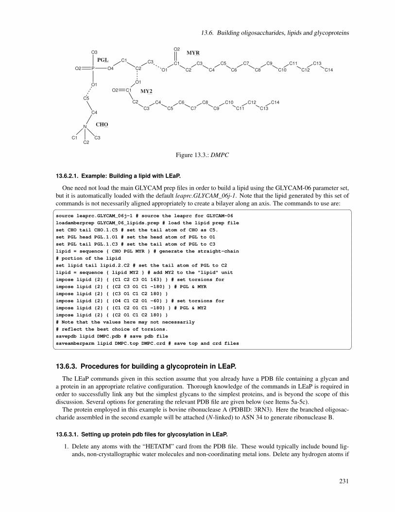
13.6. Building oligosaccharides, lipids and glycoproteins
O1
C1
C2
C3
C4
C5
C6
C7
C8
C9
C10
O2
C1
C2
C3
C4
C5
C6
C7
C8
C9
C2
C3
O1
O2
C11
C12
C13
C14
C10
C11
C12
C13
C14
C1
O4PO2
O3
O1
C5
C4
N
C2
C1 C3
MY2
MYR
CHO
PGL
Figure 13.3.: DMPC
13.6.2.1. Example: Building a lipid with LEaP.
One need not load the main GLYCAM prep files in order to build a lipid using the GLYCAM-06 parameter set,but it is automatically loaded with the default leaprc.GLYCAM_06j-1. Note that the lipid generated by this set ofcommands is not necessarily aligned appropriately to create a bilayer along an axis. The commands to use are: source leaprc.GLYCAM_06j-1 # source the leaprc for GLYCAM-06
loadamberprep GLYCAM_06_lipids.prep # load the lipid prep file
set CHO tail CHO.1.C5 # set the tail atom of CHO as C5.
set PGL head PGL.1.O1 # set the head atom of PGL to O1
set PGL tail PGL.1.C3 # set the tail atom of PGL to C3
lipid = sequence CHO PGL MYR # generate the straight-chain
# portion of the lipid
set lipid tail lipid.2.C2 # set the tail atom of PGL to C2
lipid = sequence lipid MY2 # add MY2 to the "lipid" unit
impose lipid 2 C1 C2 C3 O1 163 # set torsions for
impose lipid 2 C2 C3 O1 C1 -180 # PGL & MYR
impose lipid 2 C3 O1 C1 C2 180
impose lipid 2 O4 C1 C2 O1 -60 # set torsions for
impose lipid 2 C1 C2 O1 C1 -180 # PGL & MY2
impose lipid 2 C2 O1 C1 C2 180
# Note that the values here may not necessarily
# reflect the best choice of torsions.
savepdb lipid DMPC.pdb # save pdb file
saveamberparm lipid DMPC.top DMPC.crd # save top and crd files 13.6.3. Procedures for building a glycoprotein in LEaP.
The LEaP commands given in this section assume that you already have a PDB file containing a glycan anda protein in an appropriate relative configuration. Thorough knowledge of the commands in LEaP is required inorder to successfully link any but the simplest glycans to the simplest proteins, and is beyond the scope of thisdiscussion. Several options for generating the relevant PDB file are given below (see Items 5a-5c).
The protein employed in this example is bovine ribonuclease A (PDBID: 3RN3). Here the branched oligosac-charide assembled in the second example will be attached (N-linked) to ASN 34 to generate ribonuclease B.
13.6.3.1. Setting up protein pdb files for glycosylation in LEaP.
1. Delete any atoms with the “HETATM” card from the PDB file. These would typically include bound lig-ands, non-crystallographic water molecules and non-coordinating metal ions. Delete any hydrogen atoms if
231

13. LEaP
present.
2. In general, check the protein to make sure there are no duplicate atoms in the file. This can be quickly doneby loading the protein in LEaP and checking for such warnings. In this particular example, residue 119(HIS) contained duplicate side chain atoms. Delete all but one set of duplicate atoms.
3. Check for the presence of disulfide bonds (SSBOND) by looking at the header section of the PDB file. 3RN3has four disulfide bonds, between the following pairs of cysteine residues: 26—84, 40—95, 58—110, and65—72. Change the names of these eight cysteine residues from CYS to CYX.
4. At present, it is possible to link glycans to serine, threonine, hydroxyproline and asparagine. You must re-name the amino acid in the protein PDB file manually prior to loading it into LEaP. The modified residuenames are OLS (for O-linkages to SER), OLT (for O-linkages to THR), OLP (for O-linkages to hydrox-yproline, HYP) and NLN (for N-linkages to ASN). Libraries containing amino acid residues that have beenmodified for the purpose are automatically loaded when leaprc.GLYCAM_06j-1 is sourced. See the lists oflibrary files in3.3 for more information.
5. Prepare a PDB file containing the protein and the glycan, with the glycan correctly aligned relative to theprotein surface. There are several approaches to performing this including:
a) It is often the case that one or more glycan residues are present in the experimental PDB file. In this case,a reasonable method is to superimpose the linking sugar residue in the GLYCAM-generated glycanupon that present in the experimental PDB file, and to then save the altered coordinates. If you use thismethod, remember to delete the experimental glycan from the PDB file! It is also essential to ensurethat each carbohydrate residue is separated from other residues by a TER card in the PDB file. Alsoremember to delete the terminal OH or OMe from the glycan. Alternately, the experimental glycan maybe retained in the PDB file, provided that it is renamed according to the GLYCAM 3-letter code, andthat the atom names and order in the PDB file match the GLYCAM standard. This is tedious, but willwork. Again, be sure to insert TER cards if they are missing between the protein and the carbohydrateand between the carbohydrate residues themselves.
b) Use a molecular modeling package to align the GLYCAM-generated glycan with the protein and savethe coordinates in a single file. Remember to delete the terminal OH or OMe from the glycan.
c) Use the Glycoprotein Builder tool at http://www.glycam.org. This tool allows the user to upload proteincoordinates, build a glycan (or select it from a library), and attach it to the protein. All necessaryAMBER files may then be downloaded. This site is also convenient for preprocessing protein-onlyfiles for subsequent uploading to the glycoprotein builder.
13.6.3.2. Example: Adding a branched glycan to 3RN3 (N-linked glycosylation).
In this example we will assume that the glycan generated above (“branch.pdb”) has been aligned relative to theASN 34 in the protein file and that the complex has been saved as a new PDB file (e.g., as “3rn3_nlink.pdb”). Thelast amino acid residue should be VAL 124, and the glycan should be present as 4YB 125, 4YB 126, VMB 127,OMA 128 and OMA 129.
Remember to change the name of ASN 34 from ASN to NLN. For the glycan structure, ensure that each residuein the PDB file is separated by a “TER” card. The sequence command is not to be used here, and all linkages(within the glycan and to the protein) will be specified individually.
Enter the following commands into xleap (or tleap if a graphical representation is not desired). Alternately, copythe commands into a file to be sourced. source leaprc.GLYCAM_06j-1 # load the GLYCAM-06 leaprc for ff14SB
source leaprc.protein.ff14SB # load the protein force field
glyprot = loadpdb 3rn3_nlink.pdb # load protein and glycan pdb file
bond glyprot.125.O4 glyprot.126.C1 # make inter glycan bonds
bond glyprot.126.O4 glyprot.127.C1
bond glyprot.127.O6 glyprot.128.C1
232

13.6. Building oligosaccharides, lipids and glycoproteins
bond glyprot.127.O3 glyprot.129.C1
bond glyprot.34.SG glyprot.125.C1 # make glycan -- protein bond
bond glyprot.26.SG glyprot.84.SG # make disulfide bonds
bond glyprot.40.SG glyprot.95.SG
bond glyprot.58.SG glyprot.110.SG
bond glyprot.65.SG glyprot.72.SG
addions glyprot CL 0 # neutralize appropriately
solvateBox glyprot TIP3P BOX 8 # solvate the solute
savepdb glyprot 3nr3_glycan.pdb # save pdb file
saveamberparm glyprot 3nr3_glycan.top 3nr3_glycan.crd # save top, crd
quit # exit leap
233
14. Reading and modifying Amber parameter files
This chapter describes the content of Amber parameter files, along with details about ParmEd (which can beused to examine and modify prmtop files) and paramfit (which can be used to fit force fields to quantum mechanicaland other target data).
14.1. Understanding Amber parameter files
Romain M. Wolf, Jason Swails, and David A. Case
This chapter provides a short description of Amber-compatible force field parameter files is given. Only theactual data in parameter (*.dat) files are discussed. The special issue of deriving partial charges is not addressed.Also, more complex subjects dealing with parameters for implicit solvent (GB or PB) or polarisability computa-tions are skipped. This text is meant as a documentation for users who want to understand parameter files, and insome cases might be tempted to change or add some parameters. Most of the following documentation is found inbits and pieces at various Amber-related sites and in tutorials or original Amber manuals and these various sourceshave been helpful to put together this hopefully concise documentation.
14.1.1. Parameter Transfers between Force Fields
Transferring parameters from one force field to another must respect the underlying functional form, the units inwhich parameters are expressed in the parameter files, and also the exact procedures on how individual parameterswere obtained. In addition, attention must be paid to the methods used to deduce partial charges. Force fieldsare self-consistent, i.e., all terms are interrelated and their actual values depend on the way they were derived.Therefore, any parameter transfer between different force fields is dangerous, even when the functional form is thesame (or looks as if it were...).
Torsion terms are the most critical. Many torsion barriers and profiles are not easily assessed experimentallyand are often deduced from ab initio quantum mechanical (QM) computations on small fragments. Since QMcalculations offer many possibilities, the exact nature of these calculations (basis sets, Hartree-Fock and/or densityfunctionals, etc.) used to derive parameters should be known.
Special care must also be applied to 1-4 interactions, i.e., interactions between atoms separated by exactly threeconsecutive bonds. Most Amber force fields for example assume that 1-4 interactions get a special treatment. Seesection 14.1.6 for details. In many other force fields, the special treatment of 1-4 interactions is either different ornon-existent. This has an immediate influence on the torsion terms and resulting conformation energies. Therefore,before transferring torsion terms, van der Waals parameters and partial charges from other force fields, check thespecial treatment of 1-4 interactions in the source and the target force field.
14.1.2. How Amber Routines Use the Parameter Files
Amber routines that perform actual calculations (sander, pmemd, etc...) do not read parameter files directly.They use a special file type, the parameter-topology file (parmtop from now on), which contains all the informationrequired by the various energy functions in the computation routines. The parmtop file is specific to the molecularsystem for which it was created and is directly related to the second required file, the coordinate file.1 Smallestchanges to the system (adding or removing atoms, or even changing the order of atoms in the coordinate file)render the parmtop useless.
1This file can be in the Amber coordinate ’crd’ file format or, for some applications, also in PDB format.
234

14.1. Understanding Amber parameter files
Although parmtop files are pure ASCII files, changing parameters directly in them by standard text editors isstrongly discouraged. In the worst case, computations will run without any warnings, but results might be totallyflawed. The safest way to generate parmtop files is to use an Amber tool like tleap that has been used, tested, andenhanced over a number of years and usually generates correct parmtop files, provided that the input is correctand that all required information is available via fragment libraries and parameter files. The latest AmberTools12.0 version (April 2012) includes the ParmEd python script of Jason Swails which is very useful to examine orpost-process parmtop files. However, only users with detailed knowledge on the exact format of parmtop filesshould dare fiddling around with this data type.
14.1.3. "*.dat" and "frcmod.*" Files
The standard parameter files with the .dat extension are located in the folder $AMBERHOME/dat/leap/parm.Adding or changing parameters directly in the parameter files delivered with an Amber distribution is not a goodidea for the following reasons: (a) you might mess up the parameter file, (b) you might have trouble to rememberand find your changes later and add confusion when publishing results, (c) subsequent updates or patches mightoverwrite your changes.
In the above mentioned folder, there are also various frcmod.* files. They have basically the same format asthe parameter *.dat files. See some of the examples provided in the Amber distributions. These files can be readinto tleap exactly like the standard *.dat files. They merge the default parameters in the *.dat file with the newparameters in the frcmod.* files. More important, if the same parameters already exist in the *.dat files, theparameters in the frcmod.* files overwrite the default *.dat parameters. This offers a handy way to add new or tochange original parameters without ever touching the default parameter files. Just make sure to read the respectivefrcmod.* files in tleap when the new or altered parameters should be used.
14.1.4. Parameters Required for Amber Force Fields
The simplest form of the Amber force field (neglecting implicit solvent or polarisation terms) uses the followingHamiltonian:
Etotal = ∑bonds
kb(r− r0)2
+ ∑angles
kθ (θ −θ0)2
+ ∑dihedrals
Vn[1+ cos(nφ − γ)]
+N−1
∑i=1
N
∑j=i+1
[Ai j
R12i j−
Bi j
R6i j+
qiq j
εRi j
](14.1)
In this equation, the terms kb,r0,kθ ,θ0,Vn,γ,Ai j,Bi j are parameters to be specified in the parameter files men-tioned in section 14.1.3 for the various Amber force fields.2 The meaning of these different parameters is outlinedin the following sections.
Equation 14.1 does not have a special term for out-of-plane motions. Amber routines handle these terms throughthe same formulation as the torsion terms (see section 14.1.6).
Partial charges (qi,q j in equation 14.1), although parameters also, do not appear in parameter files, but areassigned differently (see 14.1.7).
2Note that equation 14.1 does not use the (physically more correct) kb2 , kθ
2 , and Vn2 notations because it refers to the constants as they appear
in the actual parameter files.
235
14. Reading and modifying Amber parameter files
14.1.5. Atom Types
Amber atom types can be one or two characters long. Uppercase (standard protein and nucleotide force fields),lowercase (GAFF General Amber Force Field ), and mixed upper-lowercase (GLYCAM sugar force field) areallowed. Obviously, atom types must have a single, unique, definition.
If considering the definition a new atom type, think about the consequences. Of course, an atom type with anidentical name must not already exist in one of the standard force fields used in the Amber community. Dependingon how often and in how many combinations the atom type might occur, be also aware of the rather large numberof additional parameters that might be required. Especially for bond angles, this number can grow very rapidly.
A new atom type definition, if required, must be clear and precise. It should also be possible to treat the definitionin an automatic atom-type assignment procedure. Requiring users to visually verify and to change atom types byhand will cause trouble and will make it impossible to use the force field in automatic procedures that should notrequire user intervention for this task.
14.1.6. Bonded Interaction Terms
Bond Stretching Terms
The first row in equation 14.1 (page 235) is the harmonic term for bond stretching. In Amber-type parameterfiles, the force constant kb is given for energy values in kcal/mol, with bond lengths in Å. The following line showsan example from the GAFF force field file gaff.dat.
The bond between a sp3 carbon (c3) and a hydroxyl oxygen (oh) has a default (equilibrium) value of 1.426 Åand a force constant of 314.1 kcal/mol/Å2.
c3-oh 314.1 1.4260 SOURCE1 914 0.0129
The entrance in the parameter file starts with the definition of the bond (atomtype1 hyphen atomtype2), fol-lowed by the force constant kb (in kcal/mol/Å2) and the equilibrium bond length r0 (in Å). Only the first threefields are relevant for computations. The other fields on the line above are mainly documentation.
As stated before, atom types in Amber FFs cannot have more than two characters. But if they have only onecharacter (e.g., a carbonyl carbon atom c), entries with a one-letter atom type must look like this:
c -oh 466.4 1.3060 SOURCE1 271 0.0041
i.e., the space is after the atom type, before the hyphen.Starting with a space like on the next line might lead to problems.
c-oh 466.4 1.3060 SOURCE1 271 0.0041
This holds for all parameter file entries that use hyphens to separate atom types, i.e., also angle and torsion terms(see following sections).
Angle Bending Terms
Angle bending terms are parameterised by a force constant kθ in kcal/mol/radian2 and an equilibrium anglevalue θ0 in degrees. They have the format as shown below:
c3-c3-oh 67.720 109.430 SOURCE3 48 1.5023
The middle atom c3 is bonded to another c3 and to a hydroxyl oxygen oh. The equilibrium bond angle θ0 is 109.43degrees and the force constant is 67.720 kcal/mol/radian2. Note that internally, angle deviations are computed inπ-radian2. The parmtop files also express the default ’equilibrium’ bond angles in radians. For example, the angleof 109.43 degrees is internally represented as 1.9099 π-radians. Using degrees in the original parameter files isobviously more convenient. Anything after the third field, the equilibrium angle, is mainly documentation and notrequired.
236
14.1. Understanding Amber parameter files
Torsion Terms
The third row in equation 14.1 is the usual Fourier-series expansion for torsional terms. In Amber parameterfiles, these entries require a careful explanation:
First, many torsion terms contain generic entries, using the notation ’X’ for ’any atom’. These terms are usedwhen the parameter file does not contain more specific terms for the same torsion. They are combined withexplicit terms when present. Entries with generic ’X’ atoms must always come before the more specific ones in theparameter files.
Second, Amber parameter files use a special notation for torsions that require more than one torsional term (seeexample towards the end of section 14.1.6).
Third, the parameter file entry not only contains the torsion barrier term Vn (in kcal/mol), the phase γ (degrees)and the periodicity n, but also a divider (integer) which splits the torsion term into individual contributions foreach pair of atoms involved in the torsion.
Fourth, torsion entries can also contain information about the special scaling of 1-4 non-bonded interactions(see section 14.1.6 on page 239).
Consider the following example, the default term for the torsion around a Csp3-Csp3 single bond:
X -c3-c3-X 9 1.400 0.000 3.000 JCC,7,(1986),230
The five relevant terms on this line are:
1. the definition (X -c3-c3-X)
2. the divider (9)
3. the barrier term (1.400)
4. the phase (0.000)
5. the periodicity (3.000)
Fields after the periodicity are mainly comment, except for the special flags SCNB and SCEE, that, if present,govern the special treatment of 1-4 non-bonded interaction (see section 14.1.6)
The torsional barrier term (the actual barrier divided by two) is 1.400 and the periodicity is 3. The phase is zeroin this example, meaning that a maximum energy is encountered at zero degrees. A phase of 180 degrees on theother hand means that there is a minimum at 180 degrees. The divider is 9 because each Csp3 has three X attachedto it and each X ’sees’ three X attached to the other Csp3 (3 × 3 = 9).
For a torsion angle φ (defined as X-c3-c3-X) of -60, 60, or 180 degrees, the torsion energy term would be zero:
1.49× [1+ cos(3×φ −0.0)] = 0 (14.2)
This corresponds to the staggered conformation, i.e., the lowest energy state in a X3C-CX3 connectivity like forexample ethane (H3C-CH3)
By rotating around the C-C bond, an eclipsed conformation where the X are exactly opposed is encounteredthree times (periodicity = 3), namely at φ = 0, 120, or 240 (-120) degrees.
1.49× [1+ cos(3×φ −0.0)] = 0.3111 (14.3)
.Since the divider is 9, we have to multiply the value of 0.3111 by 9 to get the full torsional barrier, i.e., 9×
0.3111 = 2.8 kcal/mol.3 This might be used for ethane for example and would be close to the experimental torsionbarrier (ca. 3 kcal/mol).
In GAFF however, there is also a specific term for hc-c3-c3-hc that would come into play for ethane. In thiscase, the divider is 1, because the term is fully defined.
3The actual barrier value of 2.8 kcal/mol here is twice the barrier term of 1.4 in the parameter file.
237

14. Reading and modifying Amber parameter files
hc-c3-c3-hc 1 0.15 0.0 3. Junmei et al, 1999
Thus, using GAFF for ethane, this term counts 9 times because there are nine [hc,hc] pairs seeing each other.Instead of equation 14.3, one would use
0.15× [1+ cos(3×φ −0.0)] = 0.3000 (14.4)
i.e., the total torsional term in ethane would be 9×0.3 = 2.7 kcal/mol. The experimental torsional barrier valueof ca. 3 kcal/mol would be reached because of the additional van der Waals and Coulomb repulsion terms betweenthe staggered hydrogens.
Assume a connectivity for which some terms are fully defined (all four atom types are specified) while nospecific entry is given for others. In that case, the equations are combined. The specific terms are counted once(divider = 1) and the remaining general terms are added according to
Vbarrier
divider× [1+ cos(periodicity×φ − phase)] (14.5)
Things get more complex when the Fourier series has more than one term. A typical example would be therotation around an amide bond R1-NH-C(=O)-R2. In this case, the trans amide (H and O on opposite sides,φ = 180) is preferred over the cis-amide (H and O on the same side, φ = 0). The entry in the GAFF parameterfile for this torsion is
hn-n -c -o 1 2.50 180.0 -2. JCC,7,(1986),230hn-n -c -o 1 2.00 0.0 1. J.C.cistrans-NMA
If the torsion definition has a "negative" periodicity (-2 in the case above), it tells programs reading the parameterfile that additional terms are present for that particular connectivity. The equation to be applied for hn-n -c -o is:
Etorsion = 2.00× [1+ cos(1×φ −0.0)]+2.50× [1+ cos(2×φ −180.0)] (14.6)
Equation 14.6 prefers the trans amide (φ = 180) over the cis amide (φ = 0) by 4 kcal/mol considering thetorsion term alone. However the more favourable Coulomb term (the 1-4 attractive interaction between the negativecarbonyl oxygen and the positive amide hydrogen) reduces the overall preference for the trans conformation closeto the experimental value of ca. 2 kcal/mol.
In addition, the following general terms have to be applied for the torsions involving R1 and R2 in the peptidebond R1-NH-C(=O)-R2, in order to compute the high torsional barrier of an amide bond:
X -c -n -X 4 10.000 180.000 2.000
Torsional terms are obviously the most difficult part to parametrize in a force field. They are in a way the lastrescue to get torsional barriers right, after all other terms have been adjusted. Therefore, their transfer from oneforce field to the other is always most risky and acceptable only if all other involved terms in two force fields arevery similar. Transferability must always be validated.
Out-of-Plane Terms
Out-of-plane terms are handled via a Fourier term, similar to the torsion terms. But the four involved atoms arenot serially (linearly) bonded, they are "branched". The "central" atom is the atom that is forced into the plane ofthe other three. For example, to keep a carbonyl group R1-C(=O)-R2 planar, the central C atom must be forcedinto the plane of the other three connected items R1, R2, and O. The entry in the GAFF parameter file for thisterm is
X -X -c -o 10.5 180. 2. JCC,7,(1986),230
Note that in Amber the central atom type (here c) is the third in the definition.The order of the remaining atomsshould (by definition) be alphabetic in atom type. The phase is always 180. In all-atom force fields, the periodicityis always 2.
Out-of-plane terms are the only terms that are allowed to be "missing" in Amber parameter files. Common onesare added automatically by tools like tleap. In many cases, these terms are "cosmetics" that avoid "in principle"
238

14.1. Understanding Amber parameter files
planar structures from getting distorted under the influence of other forces (e.g., fused rings, planar nitrogenswith three substituents, etc...). The actual parameterisation is often intuitive and for many entries, the ("generic")parameters are identical.
1-4 Non-Bonded Interaction Scaling
Figure 14.1.: 1-4 Interactions between atoms "1" and "4".
Non-bonded interactions between atoms separated by three consecutive bonds (as schematically shown in Figure14.1) require a special treatment in Amber force fields. Although referring to non-bonded interactions, scalinginformation is included in the torsion terms part of the parameter files.
By default, vdW 1-4 interactions are divided (scaled down) by a factor of 2.0, electrostatic 1-4 terms by afactor of 1.2. These are default values for the protein force fields and GAFF, but not for sugar force fields GLY-CAM_06EP and GLYCAM_06, for example, in which these interactions are not scaled at all.
Without any additional information, programs like tleap, used to prepare parmtop files, assume that thestandard scaling mentioned above is to be applied. However, this default can be overwritten in the torsion sectionof the parameter file. An example is shown below for torsional terms in the GLYCAM_06j force field:
S -Ng-Cg-H1 1 2.00 0.0 1. SCEE=1.0 SCNB=1.0 N-Sulfates
S -Ng-Cg-Cg 1 0.0 0.0 -3. SCEE=1.0 SCNB=1.0 N-Sulfates
The special notation SCEE=1.0 SCNB=1.0 following the standard torsion terms4 will tell tleap to prepare aparmtop file which transfers these data into a special section, as shown below:
%FLAG SCEE_SCALE_FACTOR
%FORMAT(5E16.8)
scaling factors are entered here....
%FLAG SCNB_SCALE_FACTOR
%FORMAT(5E16.8)
scaling factors are entered here....
When using standard Amber force field parameter files as delivered with AmberTools, the user does not need tocare about this. However, when adding additional parameters, especially torsion terms, one should be aware ofthese scaling factors and decide if they should be default or altered.
14.1.7. Non-Bonded Terms
Van der Waals Parameters
The standard formulation of the 6-12 Lennard-Jones potential Vi, j between two atoms i and j is:
4In this case, the fields coming after the periodicity (field 5), i.e., fields 6 and 7 are also read and are not ’just’ comment!
239

14. Reading and modifying Amber parameter files
Vi, j = 4εi, j
[(σi, j
ri, j
)12
−(
σi, j
ri, j
)6]
(14.7)
Here, ri, j is the distance separating the two atoms, εi, j is the depth of the potential well for the interaction ofatoms i and j, and σi, j is the distance where the potential is exactly zero, i.e., where ’repulsion’ starts for the twoatoms. Both εi, j and σi, j are specific for the pair of atoms (or more precisely, ’atom types’).
Another possible formulation of Vi, j, relating to the concept of van der Waals radii, is:
Vi, j = εi, j
[(Rmin
ri, j
)12
−2(
Rmin
ri, j
)6]
(14.8)
In this case, Rmin is the sum of the van der Waals radii, Ri +R j of atoms i and j, the contact distance at whichthe potential is at its minimum, i.e., at a value of −ε .
Figure 14.2.: Example of Lennard-Jones potential: the used data are those for the c3 atom type in the gaff forcefield (vdW radius Rmin= 1.908 Å, ε = 0.1094 kcal/mol)
Combining equations (14.7) and (14.8) gives for the relation between σ and Rmin:
Rmin = 21/6σ or σ = 2−1/6Rmin (14.9)
In force fields, the ’A,B’ notation of the Lennard-Jones potential is commonly used:
Vi, j =Ai, j
r12i, j−
Bi, j
r6i, j
(14.10)
where Ai, j and Bi, j are specific parameters for atom type pairs i and j. The meaning of Ai, j and Bi, j are easilydeduced from equation (14.7):
A = 4εσ12 and B = 4εσ
6 (14.11)
or, in terms of Rmin, using equation (14.8):
A = εR12min and B = 2εR6
min (14.12)
Van der Waals data in Amber force fields are given for each atom as a single data pair, a radius Rmin (’van derWaals’ radius in Å) and an energy ε (kcal/mol) representing the depth of the potential well.
240

14.1. Understanding Amber parameter files
These values are given at the end of the force field parameter files. In protein force fields, lines above these datashow equivalences. For example the line
N NA N2 N* NC NB NT NY
indicates that all atom types following N (the amide nitrogen) inherit the same Lennard-Jones parameters. Thus,no entry for NA, N2, ... has to be given explicitly.
For Amber force fields, cross terms involving different atom types i and j are evaluated according to theLorentz/Berthelot mixing rules:
σi, j = 0.5(σi,i +σ j, j) or Rmin,i, j = 0.5(Rmin,i +Rmin, j) (14.13)
εi, j =√
εi,i · ε j, j (14.14)
The parmtop file entries are in ’A’ and ’B’ terms to be used directly with equation 14.10, transforming the[Rmin,ε] data pairs from the parameter files.
As an example, consider ethanol (CH3CH2OH) with the GAFF force field. There are five different GAFF atomtypes. Below are shown the corresponding [Rmin,ε] data pairs, as found in the gaff.dat parameter file:
h1 1.3870 0.0157 Veenstra et al JCC,8,(1992),963
hc 1.4870 0.0157 OPLS
ho 0.0000 0.0000 OPLS Jorgensen, JACS,110,(1988),1657
oh 1.7210 0.2104 OPLS c3 1.9080 0.1094 OPLS
Note that there are three different hydrogen types: hc, the default H atom connected to an aliphatic carbon, h1, ahydrogen type connected to an aliphatic carbon with one electronegative substituent (the oxygen in this case), andthe hydroxyl hydrogen ho (for which van der Waals interactions are neglected in Amber).
Partial Charges
For Amber force fields, partial charges do not appear in parameter files. For proteins and nucleic acid force fieldsthat use fragment (residue) libraries, partial charges are pre-defined and have been computed from electrostatic-potential fitting of high-level an initio QM. They are automatically assigned by tools like tleap. Library files arefound the folder $AMBERHOME/dat/leap/lib.
Below is shown the alanine (ALA) residue of the library file all_amino94.lib:
"N" "N" 0 1 131072 1 7 -0.415700
"H" "H" 0 1 131072 2 1 0.271900
"CA" "CT" 0 1 131072 3 6 0.033700
"HA" "H1" 0 1 131072 4 1 0.082300
"CB" "CT" 0 1 131072 5 6 -0.182500
"HB1" "HC" 0 1 131072 6 1 0.060300
"HB2" "HC" 0 1 131072 7 1 0.060300
"HB3" "HC" 0 1 131072 8 1 0.060300
"C" "C" 0 1 131072 9 6 0.597300
"O" "O" 0 1 131072 10 8 -0.567900
The partial charges for each atom are given in the last field of each line.For the GAFF force field, there are various options to compute partial charges, the AM1-BBC method being
probably the best trade-off between quality and speed. There are other file types that can contain user-specifiedpartial charges, e.g., SYBYL mol2 files. See the antechamber documentation for details.
In parmtop files, partial charges are not entered as fragments of the electron charge, but are multiplied by thesquare-root of 332.05 (= 18.22), because the factor 332.05 converts the Coulomb energy into kcal/mol when usingfragments of the electron charge in the Coulomb term of equation 14.1.
241

14. Reading and modifying Amber parameter files
14.1.8. Final Remarks
Most parameters in Amber force fields have been tested on a large variety of structures. In rare cases, situationsare encountered where structures look "strange" or where results are obviously wrong. One should first lookinto details of the simulation conditions and settings before blaming the problem on actually flawed force fieldparameters. Simple test cases are often helpful to resolve the enigma.
When changing or adding parameters and later publishing results, new parameter should be mentioned. Also,the Amber developers team should be notified about possibly problematic parameters. This ensures that potentialerrors are corrected via patches in later versions and it will help the entire user community.
14.2. ParmEd
ParmEd (parmed) is a topology file editor written in Python that enables high level control of the primary forcefield file in Amber: the prmtop file. ParmEd will modify the topology file and produce a new topology file that willwork with sander, pmemd, and NAB programs, and provides options unavailable otherwise. ParmEd currentlysupports topology files created with both tleap and chamber (but support is very limited for those created withtinker_to_amber).
NOTE: The ParmEd library was reorganized following the release of AmberTools 15, which necessitated chang-ing the names of the scripts parmed.py and xparmed.py to parmed and xparmed, respectively (the .py suffix wasdropped).
14.2.1. Running parmed
parmed is used in a manner very similarly to cpptraj.
usage: parmed [-h] [-v] [-i FILE] [-p <prmtop>] [-c <inpcrd>] [-O]
[-l FILE] [--prompt PROMPT] [-n] [-e] [-s] [-r]
[<prmtop>] [<script>]
positional arguments:
<prmtop> Topology file to analyze.
<script> File with a series of ParmEd commands to execute.
optional arguments:
-h, --help show this help message and exit
-v, --version show program’s version number and exit
Input Files:
-i FILE, --input FILE
Script with ParmEd commands to execute. Default reads
from stdin. Can be specified multiple times to process
multiple input files.
-p <prmtop>, --parm <prmtop>
List of topology files to load into ParmEd. Can be
specified multiple times to process multiple
topologies.
-c <inpcrd>, --inpcrd <inpcrd>
List of inpcrd files to load into ParmEd. They are
paired with the topology files in the same order that
each set of files is specified on the command-line.
Output Files:
-O, --overwrite Allow ParmEd to overwrite existing files.
-l FILE, --logfile FILE
Log file with every command executed during an
interactive ParmEd session. Default is parmed.log
Interpreter Options:
242

14.2. ParmEd
These options affect how the ParmEd interpreter behaves in certain cases.
--prompt PROMPT String to use as a command prompt.
-n, --no-splash Prevent printing the greeting logo.
-e, --enable-interpreter
Allow arbitrary single Python commands or blocks of
Python code to be run. By default Python commands will
not be run as a safeguard for your system. Make sure
you trust the source of the ParmEd command before
turning this option on.
Error Handling:
These options control how ParmEd handles various errors and warnings that
appear occur during the course of Action execution
-s, --strict Prevent scripts from running past unrecognized input
and actions that end with an error. In interactive
mode, actions with unrecognized inputs and failed
actions prevent any changes from being made to the
topology, but does not quit the interpreter. This is
the default behavior.
-r, --relaxed Scripts ignore unrecognized input and simply skip over
failed actions, executing the rest of the script.
Unrecognized input in the interactive interpreter
emits a non-fatal warning.
Like with ptraj and cpptraj, if you do not supply the prmtop or the input_file, it will read the commands fromSTDIN as you type them.
14.2.2. ParmEd commands (they are all case-insensitive)
All actions that work on a topology file will use the “parm <idx>|<name>” input sequence to operate on aspecified topology file. If present, either the topology file loaded <idx> topologies after the first one or the topologyfile loaded with the given <name> will be modified by that action. If absent, the LAST topology file loaded willbe modified. The <idx> ranges from 0 to the total number of loaded topologies minus 1.
(Note: if you actually have a topology file named “1” that is not the second loaded topology file, you will needto address it via an index. That is, integers will always be assumed to be indices unless they are out of the topologyfile range.)
14.2.2.1. addAtomicNumber
Usage: addAtomicNumberAdds a section in the topology file with the flag ATOMIC_NUMBER in order to identify specific elements.
Elements are matched based on their atomic masses in the MASS section of the topology file. An atom is assignedan element by matching it with the element on the periodic table whose atomic mass is closest to the atom inquestion. This approach should work for any atom whose mass is either unchanged from the LEaP output or if thatatom’s mass has only been changed to one of its isotopes.
14.2.2.2. addDihedral
Usage: addDihedral <mask1> <mask2> <mask3> <mask4> <phi_k> <per> <phase> <scee> <scnb> [type<type>]
Adds a dihedral term (will NOT replace an existing dihedral) between atoms in mask1, mask2, mask3, andmask4. The dihedral is defined around the bond between the atoms in mask2 and mask3. Each mask must definethe same number of atoms. For mask1 defines atoms 1,2,3; mask2 defines atoms 11,12,13; mask3 defines atoms21,22,23; and mask4 defines atoms 31,32,33, then 3 new dihedrals will be added. One between atoms 1, 11, 21,and 31, another between atoms 2, 12, 22, and 32, and a third between atoms 3, 13, 23, and 33. The dihedrals will
243

14. Reading and modifying Amber parameter files
be set with force constant phi_k, periodicity per, phase angle phase, 1-4 electrostatic scaling factor scee (this mustbe specified – the default Amber value is 1.2 and the default GLYCAM and CHARMM value is 1.0), the 1-4 vander Waals scaling factor scnb (this must be specified – the default Amber value is 2.0 and the default GLYCAMand CHARMM value is 1.0). The type is either “normal” or “improper”. If this is an improper torsion, <mask3>should represent the central atoms bonded to all other atoms in the improper torsion.
End-group interactions are excluded automatically if the two end atoms (atoms 1 and 4) are bonded or angledto each other, or if they appear in a different dihedral. Otherwise, they are included. These are the same rulesthat tleap uses when it creates the topology file, and correctly accounts for complex exclusion rules involving ringsystems (of size 4, 5, and 6) as well as multi-term torsion parameters.
14.2.2.3. addExclusions
Usage: addExclusions <mask1> <mask2>Allows you to add arbitrary exclusions to the exclusion list. Every atom in <mask2> is added to the exclusion list
for each atom in <mask1> so that non-bonded interactions between those atom pairs will not be computed. NOTEthat this ONLY applies to direct-space (short-range) non-bonded potentials. For PME simulations, long-rangeelectrostatics between these atom pairs are still computed (in different unit cells).
14.2.2.4. addLJType
Usage: addLJType <mask> [radius <new_radius>] [epsilon <new_epsilon>] [radius_14 <new_radius14>][epsilon_14 <new_epsilon14>]
This command will assign all atoms specified in the given mask to a new van der Waals (VDW) atom type.Note that several different Amber atom types may in fact be the same VDW type, so this command is designed togive you control over changing just a single atom’s (or single Amber atom type’s) VDW parameters. Every atomspecified in the mask will be given the SAME type (but different from every other atom in the topology file), evenif their original VDW types are different. The parameters [new_radius] and [new_depth] are optional parametersthat specify that atom’s radius and well depth, which are combined with every other type’s radius and depth viathe canonical Amber combining rules. They default to the original value of the FIRST atom that is matched by themask.
Note that for chamber-created topology files (ONLY), each atom type has separate 1-4 parameters that may bespecified as well. Unspecified values will be taken from the default parameters of the first atom type as describedabove. Any attempt to supply the 1-4 parameters on a normal topology created with leap will result in an error.
See the command printLJTypes for additional information here. You can use this command to see if addLJTypemay be necessary for what you’re trying to do.
14.2.2.5. addPDB
Usage: addPDB <filename> [elem] [strict] [allicodes]This command replaces the add_pdb program that was released in previous AmberTools releases. It reads in a
PDB file <filename> and adds the following new sections to the topology file:
RESIDUE_CHAINID The chain ID of each residue (if it was added by tleap and not in the PDB file, a * is used)
RESIDUE_ICODE PDB insertion code
RESIDUE_NUMBER The original residue number of this residue in the PDB file
ATOM_ELEMENT Atomic element. This section is redundant now that the topology file has anATOMIC_NUMBER section. Therefore, this section is no longer printed by default.
The strict keyword turns residue mismatches (excluding solvent) into fatal errors. Note that for nucleic acids,terminal residue names often do not match the residue names in the PDB file because of the added 5 or 3 to theresidue name (for the 5’ terminus and 3’ terminus, respectively).
244

14.2. ParmEd
The elem keyword will force the ATOM_ELEMENT section to be printed to the topology file, but the elementwill be determined from the ATOMIC_NUMBER section (or atomic mass if the former is not present) rather thanthe atom names as was done in the add_pdb program.
The allicodes keyword forces insertion codes to be printed even if every one will be blank. This allows parsersthat use that section to be sure it will always be present.
Residues not in the PDB will be assigned a CHAINID of ’*’ and a RESIDUE_NUMBER of 0. While this actionis based on, and reproduces the key results of, the historical add_pdb program, it is a bit more flexible.
14.2.2.6. add12_6_4
Usage: add12_6_4 [<mask>] [c4file <c4file> | watermodel <watermodel>] [polfile <polfile>] [tunfactor<tunfactor>]
The add12_6_4 command is designed to create the prmtop files, which contain the C4 terms between the divalentmetal ion and every atom type. By using it together with the outparm command, there will be a new flag named"LENNARD_JONES_CCOEF" created in the end of the output prmtop file. The C4 terms between the metalions and "OW" atom type (which is the oxygen atom of the water molecule, here we assume the polarizability of"HW" is equal to zero) has been determined. Detailed information can be found in the papers of Li, Merz andco-workers.[91–93]
The C4 term between the metal ion and every other atom type is calculated by following equation:
C4(atom type) = tun f actor× C4(H2O)
α0(H2O)×α0(atom type) (14.15)
Here we explain the Usage terms:1. The <mask> is the metal ion which was treated as the metal ion center when adding the C4 terms. Please
make sure its corresponding "ATOMIC_NUMBER" is correct in the prmtop file, in that this is the criterion usedin the code to identify the metal ion. If no <mask> provided, default value :ZN.
2. To add the C4 term between the metal ion and the "OW" atom type (the oxygen atom in the water molecules),you can either use your own <c4file> (in this way you need to create a <c4file> where the first column is the AtomSymbol plus charge and the second column is the corresponding C4 value) or use the C4 values stored in parmed(in this way you only need to specify the watermodel you are using in the command line, either TIP3P, SPCE orTIP4PEW). If nothing (neither your own <c4file> nor the water model you are using) is specified, the TIP3P watermodel will be treated as the default and the related values stored in parmed will be used.
3. To add C4 terms between the metal ion and atom types besides "OW", you need a polarizability file of allthe atom types (the default file is $AMBERHOME/dat/leap/parm/lj_1264_pol.dat, you can also create and useyour own polfile where the first column is the Amber Atom Type while the second column is polarizability), anda tunfactor (which is shown in the previous equation - the default value is set as 1.0). The best tunfactor value foreach force field may be different. You can also fine tune the optimal value for a specific force field if so inclined.
After using the add12_6_4 command in the parmed, please don’t forget to use the outparm command to outputthe new prmtop file. One thing need to clarify: for the <c4file>, the first column is Atom Symbol plus charge (e.g.,Na1, Mg2, Cl-1, ...) and the second column is the C4 value between the metal ion and the "OW" atom type; forthe <polfile>, the first column is the Amber Atom Type (e.g., HC, CT, N3, OS, Be2+, Mg2+, Ca2+ ...) while thesecond column is the polarizability.
14.2.2.7. cd
This changes into the given directory (just like the UNIX cd command).
14.2.2.8. chamber
Usage: chamber -top <RTF> -param <PAR> -str <STR> -psf <PSF> [-crd <CRD>] [-nocmap] [-box<a,b,c[,α,β ,γ]>|bounding] [-radii <radiusset>]
245
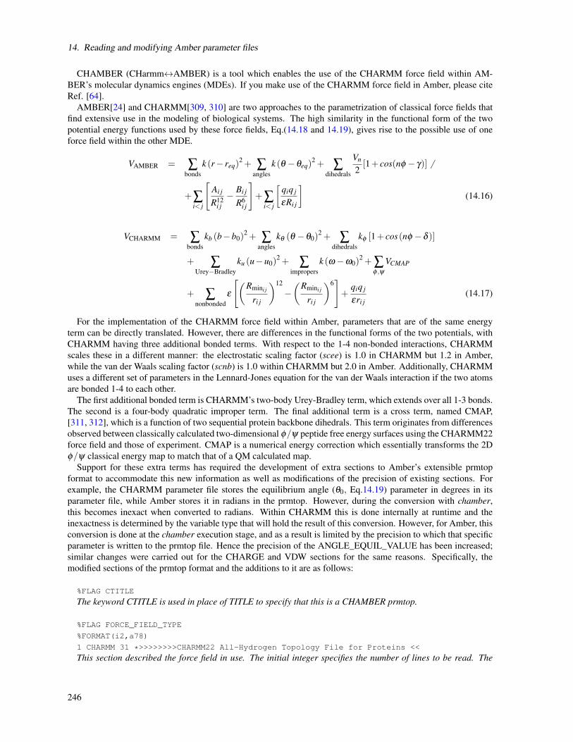
14. Reading and modifying Amber parameter files
CHAMBER (CHarmm↔AMBER) is a tool which enables the use of the CHARMM force field within AM-BER’s molecular dynamics engines (MDEs). If you make use of the CHARMM force field in Amber, please citeRef. [64].
AMBER[24] and CHARMM[309, 310] are two approaches to the parametrization of classical force fields thatfind extensive use in the modeling of biological systems. The high similarity in the functional form of the twopotential energy functions used by these force fields, Eq.(14.18 and 14.19), gives rise to the possible use of oneforce field within the other MDE.
VAMBER = ∑bonds
k (r− req)2 + ∑
anglesk (θ −θeq)
2 + ∑dihedrals
Vn
2[1+ cos(nφ − γ)] 6
+∑i< j
[Ai j
R12i j−
Bi j
R6i j
]+∑
i< j
[qiq j
εRi j
](14.16)
VCHARMM = ∑bonds
kb (b−b0)2 + ∑
angleskθ (θ −θ0)
2 + ∑dihedrals
kφ [1+ cos(nφ −δ )]
+ ∑Urey−Bradley
ku (u−u0)2 + ∑
impropersk (ω−ω0)
2 + ∑φ ,ψ
VCMAP
+ ∑nonbonded
ε
[(Rmini j
ri j
)12
−(
Rmini j
ri j
)6]+
qiq j
εri j(14.17)
For the implementation of the CHARMM force field within Amber, parameters that are of the same energyterm can be directly translated. However, there are differences in the functional forms of the two potentials, withCHARMM having three additional bonded terms. With respect to the 1-4 non-bonded interactions, CHARMMscales these in a different manner: the electrostatic scaling factor (scee) is 1.0 in CHARMM but 1.2 in Amber,while the van der Waals scaling factor (scnb) is 1.0 within CHARMM but 2.0 in Amber. Additionally, CHARMMuses a different set of parameters in the Lennard-Jones equation for the van der Waals interaction if the two atomsare bonded 1-4 to each other.
The first additional bonded term is CHARMM’s two-body Urey-Bradley term, which extends over all 1-3 bonds.The second is a four-body quadratic improper term. The final additional term is a cross term, named CMAP,[311, 312], which is a function of two sequential protein backbone dihedrals. This term originates from differencesobserved between classically calculated two-dimensional φ/ψ peptide free energy surfaces using the CHARMM22force field and those of experiment. CMAP is a numerical energy correction which essentially transforms the 2Dφ/ψ classical energy map to match that of a QM calculated map.
Support for these extra terms has required the development of extra sections to Amber’s extensible prmtopformat to accommodate this new information as well as modifications of the precision of existing sections. Forexample, the CHARMM parameter file stores the equilibrium angle (θ0, Eq.14.19) parameter in degrees in itsparameter file, while Amber stores it in radians in the prmtop. However, during the conversion with chamber,this becomes inexact when converted to radians. Within CHARMM this is done internally at runtime and theinexactness is determined by the variable type that will hold the result of this conversion. However, for Amber, thisconversion is done at the chamber execution stage, and as a result is limited by the precision to which that specificparameter is written to the prmtop file. Hence the precision of the ANGLE_EQUIL_VALUE has been increased;similar changes were carried out for the CHARGE and VDW sections for the same reasons. Specifically, themodified sections of the prmtop format and the additions to it are as follows:
%FLAG CTITLE
The keyword CTITLE is used in place of TITLE to specify that this is a CHAMBER prmtop.
%FLAG FORCE_FIELD_TYPE
%FORMAT(i2,a78)
1 CHARMM 31 *>>>>>>>>CHARMM22 All-Hydrogen Topology File for Proteins <<
This section described the force field in use. The initial integer specifies the number of lines to be read. The
246
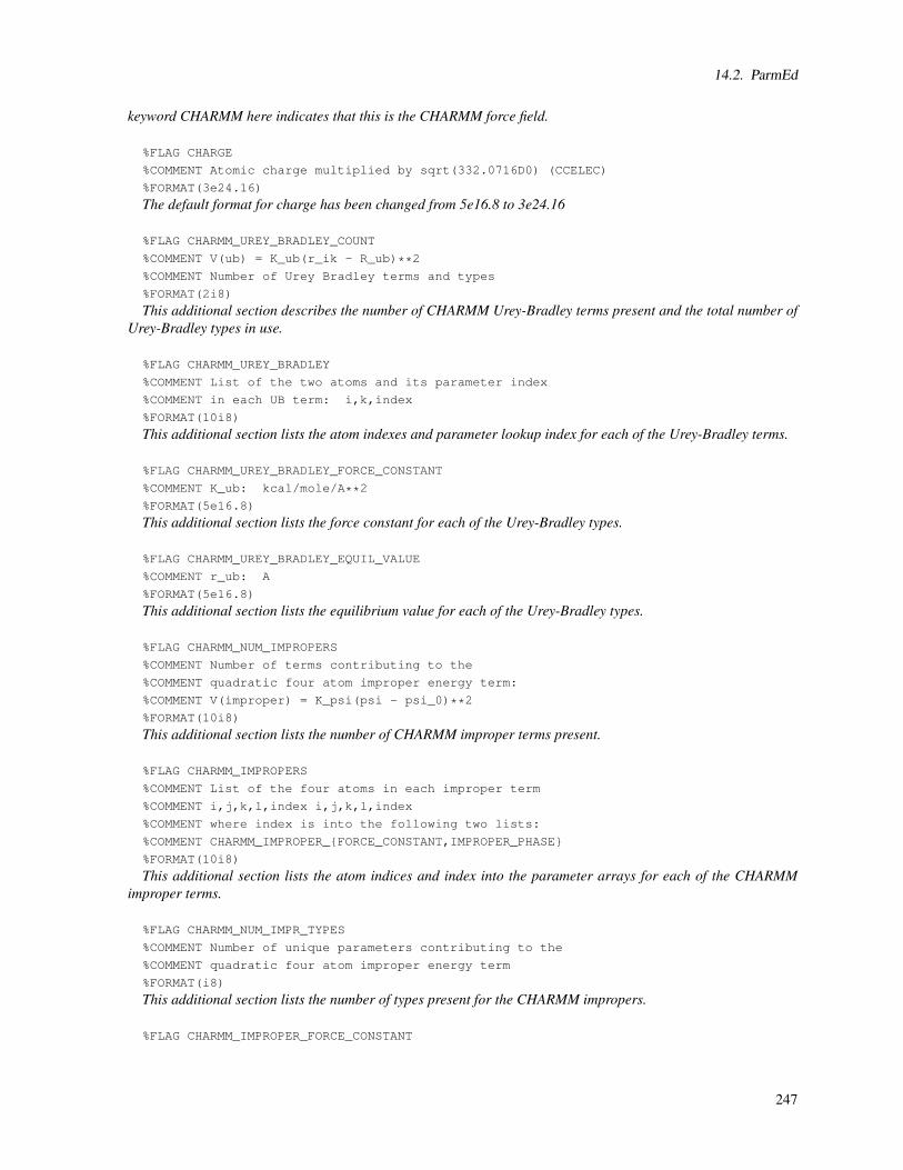
14.2. ParmEd
keyword CHARMM here indicates that this is the CHARMM force field.
%FLAG CHARGE
%COMMENT Atomic charge multiplied by sqrt(332.0716D0) (CCELEC)
%FORMAT(3e24.16)
The default format for charge has been changed from 5e16.8 to 3e24.16
%FLAG CHARMM_UREY_BRADLEY_COUNT
%COMMENT V(ub) = K_ub(r_ik - R_ub)**2
%COMMENT Number of Urey Bradley terms and types
%FORMAT(2i8)
This additional section describes the number of CHARMM Urey-Bradley terms present and the total number ofUrey-Bradley types in use.
%FLAG CHARMM_UREY_BRADLEY
%COMMENT List of the two atoms and its parameter index
%COMMENT in each UB term: i,k,index
%FORMAT(10i8)
This additional section lists the atom indexes and parameter lookup index for each of the Urey-Bradley terms.
%FLAG CHARMM_UREY_BRADLEY_FORCE_CONSTANT
%COMMENT K_ub: kcal/mole/A**2
%FORMAT(5e16.8)
This additional section lists the force constant for each of the Urey-Bradley types.
%FLAG CHARMM_UREY_BRADLEY_EQUIL_VALUE
%COMMENT r_ub: A
%FORMAT(5e16.8)
This additional section lists the equilibrium value for each of the Urey-Bradley types.
%FLAG CHARMM_NUM_IMPROPERS
%COMMENT Number of terms contributing to the
%COMMENT quadratic four atom improper energy term:
%COMMENT V(improper) = K_psi(psi - psi_0)**2
%FORMAT(10i8)
This additional section lists the number of CHARMM improper terms present.
%FLAG CHARMM_IMPROPERS
%COMMENT List of the four atoms in each improper term
%COMMENT i,j,k,l,index i,j,k,l,index
%COMMENT where index is into the following two lists:
%COMMENT CHARMM_IMPROPER_FORCE_CONSTANT,IMPROPER_PHASE
%FORMAT(10i8)
This additional section lists the atom indices and index into the parameter arrays for each of the CHARMMimproper terms.
%FLAG CHARMM_NUM_IMPR_TYPES
%COMMENT Number of unique parameters contributing to the
%COMMENT quadratic four atom improper energy term
%FORMAT(i8)
This additional section lists the number of types present for the CHARMM impropers.
%FLAG CHARMM_IMPROPER_FORCE_CONSTANT
247

14. Reading and modifying Amber parameter files
%COMMENT K_psi: kcal/mole/rad**2
%FORMAT(5e16.8)
This additional section lists the force constant for each CHARMM improper types.
%FLAG CHARMM_IMPROPER_PHASE
%COMMENT psi: degrees
%FORMAT(5e16.8)
This additional section lists the equilibrium phase angle for each of the CHARMM improper types.
%FLAG LENNARD_JONES_ACOEF
%FORMAT(3e24.16)
The default format for the Lennard Jones A and B coefficients has been changed from 5e16.8 to 3e24.16.
%FLAG LENNARD_JONES_14_ACOEF
%FORMAT(3e24.16)
This additional section and the corresponding BCOEF section provide the alternative parameters for 1-4 VDWinteractions in the CHARMM force field.
In concert with these prmtop additions, the appropriate modifications have to be made within sander and pmemdto enable the calculation of the energy and derivatives corresponding to these new terms. The intention behind theapproach of creating a CHARMM enabled prmtop file is that the use of this prmtop file should be transparentto the user. Once a CHARMM prmtop file is produced by chamber, the sander and pmemd dynamics enginesautomatically detect the presence of CHARMM parameters in the prmtop file and automatically select the correctparameters and code paths.
WARNING: The use of an unpatched Amber molecular dynamics engine with a chamber-generated prmtop filewill give undefined behavior, leading to incorrect results. If you see the following error at runtime:
ERROR: Flag "TITLE" not found in PARM file
it most likely means that you are using an old pmemd or sander executable.
CHAMBER (CHarmm↔AMBER) is a tool which enables the use of the CHARMM force field within AM-BER’s molecular dynamics engines (MDEs). If you make use of the CHARMM force field in Amber, please citeRef. [64].
AMBER[24] and CHARMM[309, 310] are two approaches to the parametrization of classical force fields thatfind extensive use in the modeling of biological systems. The high similarity in the functional form of the twopotential energy functions used by these force fields, Eq.(14.18 and 14.19), gives rise to the possible use of oneforce field within the other MDE.
VAMBER = ∑bonds
k (r− req)2 + ∑
anglesk (θ −θeq)
2 + ∑dihedrals
Vn
2[1+ cos(nφ − γ)] 6
+∑i< j
[Ai j
R12i j−
Bi j
R6i j
]+∑
i< j
[qiq j
εRi j
](14.18)
VCHARMM = ∑bonds
kb (b−b0)2 + ∑
angleskθ (θ −θ0)
2 + ∑dihedrals
kφ [1+ cos(nφ −δ )]
+ ∑Urey−Bradley
ku (u−u0)2 + ∑
impropersk (ω−ω0)
2 + ∑φ ,ψ
VCMAP
+ ∑nonbonded
ε
[(Rmini j
ri j
)12
−(
Rmini j
ri j
)6]+
qiq j
εri j(14.19)
248
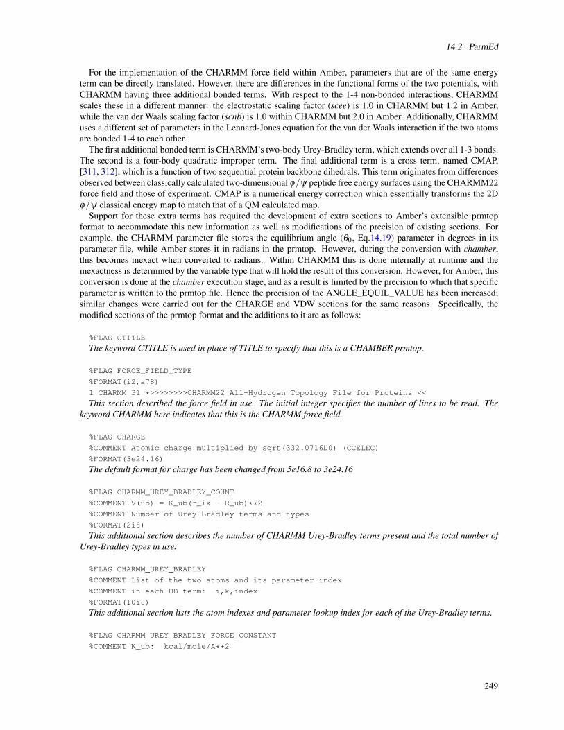
14.2. ParmEd
For the implementation of the CHARMM force field within Amber, parameters that are of the same energyterm can be directly translated. However, there are differences in the functional forms of the two potentials, withCHARMM having three additional bonded terms. With respect to the 1-4 non-bonded interactions, CHARMMscales these in a different manner: the electrostatic scaling factor (scee) is 1.0 in CHARMM but 1.2 in Amber,while the van der Waals scaling factor (scnb) is 1.0 within CHARMM but 2.0 in Amber. Additionally, CHARMMuses a different set of parameters in the Lennard-Jones equation for the van der Waals interaction if the two atomsare bonded 1-4 to each other.
The first additional bonded term is CHARMM’s two-body Urey-Bradley term, which extends over all 1-3 bonds.The second is a four-body quadratic improper term. The final additional term is a cross term, named CMAP,[311, 312], which is a function of two sequential protein backbone dihedrals. This term originates from differencesobserved between classically calculated two-dimensional φ/ψ peptide free energy surfaces using the CHARMM22force field and those of experiment. CMAP is a numerical energy correction which essentially transforms the 2Dφ/ψ classical energy map to match that of a QM calculated map.
Support for these extra terms has required the development of extra sections to Amber’s extensible prmtopformat to accommodate this new information as well as modifications of the precision of existing sections. Forexample, the CHARMM parameter file stores the equilibrium angle (θ0, Eq.14.19) parameter in degrees in itsparameter file, while Amber stores it in radians in the prmtop. However, during the conversion with chamber,this becomes inexact when converted to radians. Within CHARMM this is done internally at runtime and theinexactness is determined by the variable type that will hold the result of this conversion. However, for Amber, thisconversion is done at the chamber execution stage, and as a result is limited by the precision to which that specificparameter is written to the prmtop file. Hence the precision of the ANGLE_EQUIL_VALUE has been increased;similar changes were carried out for the CHARGE and VDW sections for the same reasons. Specifically, themodified sections of the prmtop format and the additions to it are as follows:
%FLAG CTITLE
The keyword CTITLE is used in place of TITLE to specify that this is a CHAMBER prmtop.
%FLAG FORCE_FIELD_TYPE
%FORMAT(i2,a78)
1 CHARMM 31 *>>>>>>>>CHARMM22 All-Hydrogen Topology File for Proteins <<
This section described the force field in use. The initial integer specifies the number of lines to be read. Thekeyword CHARMM here indicates that this is the CHARMM force field.
%FLAG CHARGE
%COMMENT Atomic charge multiplied by sqrt(332.0716D0) (CCELEC)
%FORMAT(3e24.16)
The default format for charge has been changed from 5e16.8 to 3e24.16
%FLAG CHARMM_UREY_BRADLEY_COUNT
%COMMENT V(ub) = K_ub(r_ik - R_ub)**2
%COMMENT Number of Urey Bradley terms and types
%FORMAT(2i8)
This additional section describes the number of CHARMM Urey-Bradley terms present and the total number ofUrey-Bradley types in use.
%FLAG CHARMM_UREY_BRADLEY
%COMMENT List of the two atoms and its parameter index
%COMMENT in each UB term: i,k,index
%FORMAT(10i8)
This additional section lists the atom indexes and parameter lookup index for each of the Urey-Bradley terms.
%FLAG CHARMM_UREY_BRADLEY_FORCE_CONSTANT
%COMMENT K_ub: kcal/mole/A**2
249

14. Reading and modifying Amber parameter files
%FORMAT(5e16.8)
This additional section lists the force constant for each of the Urey-Bradley types.
%FLAG CHARMM_UREY_BRADLEY_EQUIL_VALUE
%COMMENT r_ub: A
%FORMAT(5e16.8)
This additional section lists the equilibrium value for each of the Urey-Bradley types.
%FLAG CHARMM_NUM_IMPROPERS
%COMMENT Number of terms contributing to the
%COMMENT quadratic four atom improper energy term:
%COMMENT V(improper) = K_psi(psi - psi_0)**2
%FORMAT(10i8)
This additional section lists the number of CHARMM improper terms present.
%FLAG CHARMM_IMPROPERS
%COMMENT List of the four atoms in each improper term
%COMMENT i,j,k,l,index i,j,k,l,index
%COMMENT where index is into the following two lists:
%COMMENT CHARMM_IMPROPER_FORCE_CONSTANT,IMPROPER_PHASE
%FORMAT(10i8)
This additional section lists the atom indices and index into the parameter arrays for each of the CHARMMimproper terms.
%FLAG CHARMM_NUM_IMPR_TYPES
%COMMENT Number of unique parameters contributing to the
%COMMENT quadratic four atom improper energy term
%FORMAT(i8)
This additional section lists the number of types present for the CHARMM impropers.
%FLAG CHARMM_IMPROPER_FORCE_CONSTANT
%COMMENT K_psi: kcal/mole/rad**2
%FORMAT(5e16.8)
This additional section lists the force constant for each CHARMM improper types.
%FLAG CHARMM_IMPROPER_PHASE
%COMMENT psi: degrees
%FORMAT(5e16.8)
This additional section lists the equilibrium phase angle for each of the CHARMM improper types.
%FLAG LENNARD_JONES_ACOEF
%FORMAT(3e24.16)
The default format for the Lennard Jones A and B coefficients has been changed from 5e16.8 to 3e24.16.
%FLAG LENNARD_JONES_14_ACOEF
%FORMAT(3e24.16)
This additional section and the corresponding BCOEF section provide the alternative parameters for 1-4 VDWinteractions in the CHARMM force field.
In concert with these prmtop additions, the appropriate modifications have to be made within sander and pmemdto enable the calculation of the energy and derivatives corresponding to these new terms. The intention behind theapproach of creating a CHARMM enabled prmtop file is that the use of this prmtop file should be transparentto the user. Once a CHARMM prmtop file is produced by chamber, the sander and pmemd dynamics engines
250

14.2. ParmEd
automatically detect the presence of CHARMM parameters in the prmtop file and automatically select the correctparameters and code paths.
WARNING: The use of an unpatched Amber molecular dynamics engine with a chamber-generated prmtop filewill give undefined behavior, leading to incorrect results. If you see the following error at runtime:
ERROR: Flag "TITLE" not found in PARM file
it most likely means that you are using an old pmemd or sander executable.
This command will read topology information from a CHARMM or XPLOR PSF file and write an AMBERinpcrd and chamber-style prmtop file so the CHARMM force field can be run in sander and pmemd. PSF filesgenerated by CHARMM, CHARMM-GUI, and VMD are all supported. PSF files are always generated using a setof topology (RTF) files that define the residues (akin to library files in tleap)—these files define the connectivityand atom types of all atoms in the system. Topology and parameter (PAR) files are always paired, so you must usethe parameter file here that matches the topology file you used to create the PSF originally. This is very important.CHARMM stream files (that define both residue and parameter sections) are also supported, but must be specifiedusing the -str flag. Do not pass any topology or parameter files to the -str flag. The -top and -param flags can bespecified multiple times.
NBFIX terms defined in any stream or parameter files are read and implemented.
-top <RTF> CHARMM Residue Topology File (RTF). This is not needed if the atom types are defined in theparameter files (this seems to be true for CHARMM36 and probably later force fields).
-par <PAR> CHARMM Parameter file. This defines all of the CHARMM parameter files, and the one that corre-sponds to the topology file used to create the PSF must be used.
-str <STR> CHARMM stream file. Any parameters stored in the stream file will be loaded.
-toppar <RTF|PAR> CHARMM RTF, parameter, or stream file—the type is automatically detected from the name.All standard CHARMM files should work, but if you have changed the file name, you should use eitherthe -top, -par, or -str flags above. Wild-cards are recognized, so you can do something like -toppar
toppar/*36_prot* to get all of the files that contain 36_prot in their name inside the toppar directory.
-psf <PSF> CHARMM/XPLOR/VMD Protein Structure File (PSF). This file defines the structure and topologyof the system.
-crd <CRD> File containing coordinates for the system. CHARMM coordinate, restart, and PDB files are allsupported. If this is a PDB file and a CRYST1 record defines a periodic box, the unit cell dimensions willbe set from this information. You can use the -box argument to override this.
-nocmap Ignore any CMAP terms that may be defined. This is strongly discouraged unless you have a goodreason to do it.
-box <a,b,c[,α,β ,γ]>|bounding Defines the periodic box dimensions (and will override any PBC defined in thecoordinate file). You can either give the keyword “bounding,” which will define the smallest possible or-thorhombic box that encloses the centers of all atoms or you can give the unit cell dimensions. If you provideonly lengths, the box shape is assumed to be orthorhombic.
-radii <radiusset> The AMBER implicit solvent radius set. The options are equivalent to the “set PBRadii <ra-diusset>” options in tleap. See page 221 for more information. Available choices are amber6, bondi, mbondi,mbondi2, and mbondi3. Default choice is “mbondi” (same as tleap).
Note, after using this command, the created parm object will be the active parm. You need to use either the parmoutor outparm commands to actually print a topology file (and don’t forget to also print a coordinate file!)
251

14. Reading and modifying Amber parameter files
14.2.3. Validation
Starting with version c36a2 of CHARMM, a command (frcdump) has been implemented which provides avalidation route for alternate implementations of the CHARMM force fields. For a given system, this commandwrites the various force field potential energy contributions, as well as the energy gradient experienced by eachatom, to a file using a specific format and to a high precision. The same formatted output can also be generated bythe AMBER MDEs to facilitate comparison and to validate that the CHARMM force field is being implementedcorrectly in Amber’s MDEs.
An example section of a charmm script that will write this output to a file called charmm_gold_c36a2 is asfollows:
open unit 20 form write name charmm_gold_c36a2
frcdump unit 20
close unit 20
The analogous mdin section for Amber is as follows:
&debugf
do_charmm_dump_gold = 1,
/
Given this directive, the Amber MDE will stop after evaluating the potential energy of a system and write theenergy and forces pertaining to this to a (hardcoded) file called charmm_gold in the same directory as the mdinfile. The reader is invited to examine the various example test calculations within the $AMBERHOME/test/cham-ber/dev_tests/ directory for in depth examples of the above. For such testing, it is recommended that both theCHARMM binary and the Amber MDE binaries be compiled with the same compiler. Given that CHARMMsupport within Amber and the chamber software is still somewhat experimental, the user is advised to carry outsuch a comparison before running a long production run.
14.2.4. Known limitations / Issues
This is a non-exhaustive list of the current known bugs and/or limitations with chamber:
• CHARMM polarization models are not supported. (IPOL /= 0)
• The mdout file will contain extra potential energy fields pertaining to the CHARMM terms. This may breakor confuse third party scripts that parse such outputs.
• Third party scripts and/or tools which do not correctly parse the extensible prmtop format may have issueswith a chamber-generated prmtop file.
• The potential energy decomposition components (self, reciprocal, direct, adjusted) of the Particle MeshEwald energy generated in the charmm_gold file when the do_charmm_dump_gold = 1 mdin option inAmber do not match with the breakdown used in CHARMM, however, the summation and resulting forcesdo match.
If other issues are found, the parmed authors would be very grateful if these could be reported to them, either viathe Amber mailing list and/or directly to the authors. Please ensure that prior to reporting an issue, the chamberbinary passes the test cases provided with AmberTools. Please provide a standalone example of the problem withall input files present and a script reproducing the sequence of commands that triggers the problem. The postingof large files (> 2 MB) to the Amber mailing list is not recommended; instead one should make the files availableon a website somewhere and provide a link to it with the posting to the list.
252
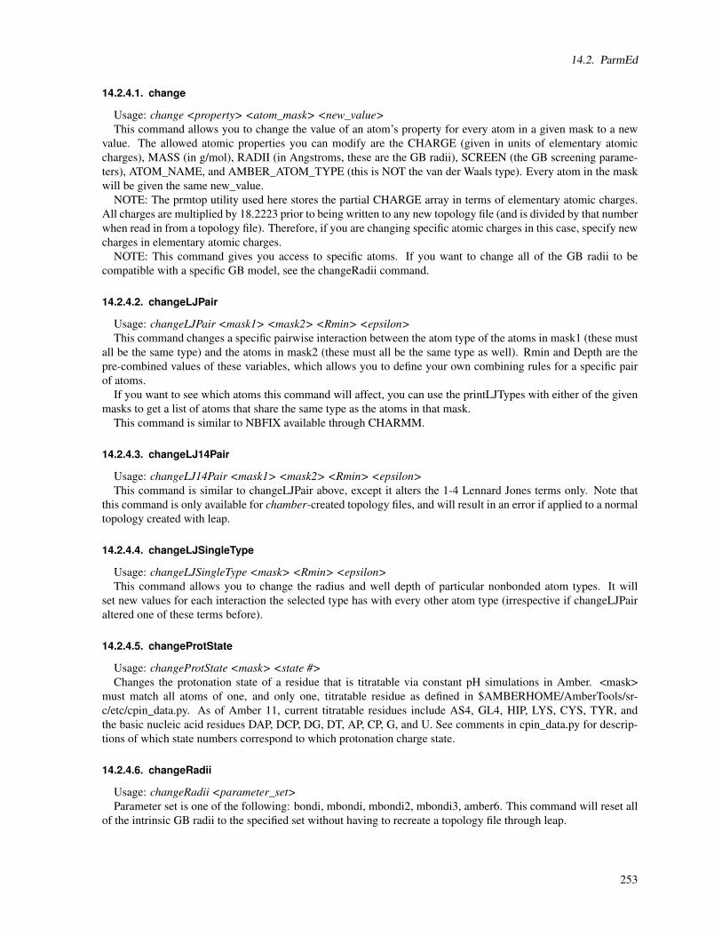
14.2. ParmEd
14.2.4.1. change
Usage: change <property> <atom_mask> <new_value>This command allows you to change the value of an atom’s property for every atom in a given mask to a new
value. The allowed atomic properties you can modify are the CHARGE (given in units of elementary atomiccharges), MASS (in g/mol), RADII (in Angstroms, these are the GB radii), SCREEN (the GB screening parame-ters), ATOM_NAME, and AMBER_ATOM_TYPE (this is NOT the van der Waals type). Every atom in the maskwill be given the same new_value.
NOTE: The prmtop utility used here stores the partial CHARGE array in terms of elementary atomic charges.All charges are multiplied by 18.2223 prior to being written to any new topology file (and is divided by that numberwhen read in from a topology file). Therefore, if you are changing specific atomic charges in this case, specify newcharges in elementary atomic charges.
NOTE: This command gives you access to specific atoms. If you want to change all of the GB radii to becompatible with a specific GB model, see the changeRadii command.
14.2.4.2. changeLJPair
Usage: changeLJPair <mask1> <mask2> <Rmin> <epsilon>This command changes a specific pairwise interaction between the atom type of the atoms in mask1 (these must
all be the same type) and the atoms in mask2 (these must all be the same type as well). Rmin and Depth are thepre-combined values of these variables, which allows you to define your own combining rules for a specific pairof atoms.
If you want to see which atoms this command will affect, you can use the printLJTypes with either of the givenmasks to get a list of atoms that share the same type as the atoms in that mask.
This command is similar to NBFIX available through CHARMM.
14.2.4.3. changeLJ14Pair
Usage: changeLJ14Pair <mask1> <mask2> <Rmin> <epsilon>This command is similar to changeLJPair above, except it alters the 1-4 Lennard Jones terms only. Note that
this command is only available for chamber-created topology files, and will result in an error if applied to a normaltopology created with leap.
14.2.4.4. changeLJSingleType
Usage: changeLJSingleType <mask> <Rmin> <epsilon>This command allows you to change the radius and well depth of particular nonbonded atom types. It will
set new values for each interaction the selected type has with every other atom type (irrespective if changeLJPairaltered one of these terms before).
14.2.4.5. changeProtState
Usage: changeProtState <mask> <state #>Changes the protonation state of a residue that is titratable via constant pH simulations in Amber. <mask>
must match all atoms of one, and only one, titratable residue as defined in $AMBERHOME/AmberTools/sr-c/etc/cpin_data.py. As of Amber 11, current titratable residues include AS4, GL4, HIP, LYS, CYS, TYR, andthe basic nucleic acid residues DAP, DCP, DG, DT, AP, CP, G, and U. See comments in cpin_data.py for descrip-tions of which state numbers correspond to which protonation charge state.
14.2.4.6. changeRadii
Usage: changeRadii <parameter_set>Parameter set is one of the following: bondi, mbondi, mbondi2, mbondi3, amber6. This command will reset all
of the intrinsic GB radii to the specified set without having to recreate a topology file through leap.
253

14. Reading and modifying Amber parameter files
14.2.4.7. checkValidity
Usage: checkValidityThoroughly checks the topology file for a wide range of errors. It also checks for common mistakes, like missing
disulfide bridges, for instance. More checks are done if a restart file is loaded prior to running this command. Ifyou are getting a strange error from a simulation engine, it may be worth using this to check the prmtop. Note thatthis action, in particular, requires a version of Python 2.5 to 2.7.
14.2.4.8. defineSolvent
Usage: defineSolvent <residue_list>This command will allow you to define custom solvent residues. The residue_list must be a comma-separated
list with no whitespace separating the residue names. This is important for the proper determination of the SOL-VENT_POINTERS and ATOMS_PER_MOLECULE sections of the topology file. By default, HOH and WATresidues are recognized as solvent.
14.2.4.9. deleteBond
Usage: deleteBond <mask1> <mask2> [verbose]This command will delete all bonds in which one atom is in mask1 and the other atom is in mask2. It also deletes
all other valence terms (angles, Urey-Bradleys,* torsions, impropers, and CMAPs,*) in which a deleted bond wasa part. This is distinct from using setBond to assign a force constant of 0 because it also deletes other valenceterms and removes those atoms from the respective nonbonded exclusion lists (since they are no longer bonded toeach other).
If you use the “verbose” keyword, you will get a printout of every bond that is deleted.*Some terms are only found in chamber-style topology files specifying a CHARMM force field.
14.2.4.10. deleteDihedral
Usage: deleteDihedral <mask1> <mask2> <mask3> <mask4>Deletes the dihedral around <mask2> and <mask3> in which the end-groups are <mask1> and <mask4>. For
multi-term dihedrals, it removes each term.
14.2.4.11. deletePDB
Usage: deletePDBDeletes the flags that are added by addPDB (see description above).
14.2.4.12. energy
Usage: energy [cutoff <cut>] [[igb <IGB>] [saltcon <conc>] | [Ewald]] [nodisper] [omm] [applayer] [plat-form <platform>] [precision <precision model>] [decompose]
Computes the energy for a given structure. If you did not load a coordinate file on the command-line, you mustuse loadRestrt (see below) in order to load a set of coordinates (and box dimensions for periodic simulations). Theoptions are:
cutoff <cut> The cutoff, in Angstroms, to use for the nonbonded cutoff. The default value is 1000 for non-periodicsystems and 8 for periodic systems.
dumpfrc <filename> The file name to write atomic forces to. The format is a single header line starting with ’#’followed by natom lines with the x, y, and z components of the force space-delimited.
254

14.2. ParmEd
Non-periodic options These options are applied only to non-periodic simulations. If the prmtop indicates peri-odicity (i.e., IFBOX > 0), these options are ignored.
igb <IGB> GB model to use. Allowed values are 0, 1, 2, 5, 6, 7, and 8. The values 0 and 6 indicate vacuumelectrostatics. The other values match the options available in sander, pmemd, and NAB (see pages 57 and796 for more details).
saltcon <conc> Salt concentration (in Molarity) to use when using GB implicit solvent. See page 59 for moreinformation.
Periodic options These options are applied only to periodic simulations. If the prmtop does not indicate period-icity (i.e., IFBOX == 2), these options are ignored.
Ewald Use the Ewald sum to compute long-range electrostatics instead of Particle-Mesh Ewald (this is muchslower than PME for large systems). This is equivalent to setting ew_type=1 in sander.
nodisper Do not use the long-range dispersion correction to correct for Lennard-Jones interactions that are ex-cluded beyond the cutoff. This is equivalent to setting vdwmeth=0 in sander and pmemd.
OpenMM-specific options Instead of using the sander-Python API to compute energies and forces, you can useOpenMM. OpenMM must be installed and the Python application layer must be available for import. OpenMMcannot currently handle octahedral boxes (or any non-orthorhombic box).
omm This keyword must be present in order to use the OpenMM engine instead of the sander Python package.All following options are ignored unless this keyword is present
platform <platform> OpenMM compute platform to use. Options are CUDA, OpenCL, Reference, and CPU.Consult the OpenMM manual for more details.
precision <precision model> OpenMM precision model to use. Options are single, double, and mixed. Refer-ence is always double and CPU is always single. The mixed precision model (default) uses single precisionfor calculations and double for accumulation.
decompose By default, OpenMM does not decompose energy contributions to different terms (e.g., bond, an-gle, torsion, etc.). If present, this keyword will make ParmEd break the energies down as much as possible(OpenMM does not compute non-bonded energy terms separately, so Lennard-Jones, 1-4 nonbonded inter-actions, and electrostatics will all be conflated into a single term). Energy terms are always decomposedwhen not using the OpenMM API.
applayer If present, this keyword will write a temporary topology file and load an OpenMM system using the sup-port classes bundled with OpenMM directly (rather than using ParmEd’s internal OpenMM System creator).This is provided as a way to validate the agreement between OpenMM’s application layer and ParmEd.
14.2.4.13. go
Usage: goStop reading commands and execute every command that has come before. This has exactly the same effect as
the End Of File (EOF) character. All commands in a script after “go” will be ignored. Placing “go” as the lastline of a script is the same as not including it at all (since the next line contains EOF, which executes the samebehavior). Thus, you can get the same behavior from the interactive session by either typing “go” or sending theEOF character (which on unix is CTRL-D)
255

14. Reading and modifying Amber parameter files
14.2.4.14. gromber
Usage: gromber <top_file> [define <DEFINE[=VAR]>] [topdir <directory>] [radii <radiusset>]Load a Gromacs topology file with parameters as an Amber-formatted system. Note, if your Gromacs topology
file requires any include topology files (as most do), you will need to have Gromacs installed for this to work.
• <top_file>: The Gromacs topology file to load
• <coord_file>: The coordinate file to load into the system. Can be any recognized format (GRO, PDB,mmCIF, inpcrd, etc.)
• define <DEFINE[=VAR]>: Preprocessor defines that control the processing of the Gromacs topology file.
• topdir <directory>: The directory containing all Gromacs include topology files. This is only necessaryif Gromacs is not installed in a location that ParmEd can find.
• radii <radiusset>: The GB radius set to use. Can be mbondi, bondi, mbondi2, or amber6. Default ismbondi
Gromacs topology files do not store the unit cell information. Therefore, in order to make sure that unit cellinformation is properly assigned to the resulting system, the provided <coord_file> should contain unit cellinformation (e.g., GRO, PDB, PDBx/mmCIF, and inpcrd files can all store box information).
ParmEd will try to locate the Gromacs topology directory using either the GMXDATA or GMXBIN environmentvariables (which should point to the $PREFIX/share/gromacs or $PREFIX/bin directories, respectively, where$PREFIX is the install prefix). If neither is set, the topology directory is located relative to the location of thegmx (Gromacs 5+) or pdb2gmx (Gromacs 4 or older) in the user’s PATH. If none of the above is true, the defaultinstallation location (/usr/local/gromacs/share/gromacs/top) is used. Any provided topdir will overridedefault choices (but only for this particular command – future gromber actions will use the default location again).
You can provide as many defines as you wish, and the ordering you specify them is preserved. The defaultvalue assigned to each define is "1". To provide multiple defines, use the keyword multiple times, for example:
define MYVAR=something define MYVAR2=something_else ...
It is important to note that Gromacs supports a much larger array of bonded potentials than Amber does. Gromacssupports several different bonded potentials (cubic, quartic, and Morse, just to name a few), while Amber supportsonly the simple harmonic bond potential. Similarly, Amber only supports quadratic angle potentials, periodictorsions, and the 12-6 Lennard-Jones potential. Through the chamber extensions (see Sec. 14.2.2.8), Amber canalso support Urey-Bradley angle potentials, quadratic improper potentials, and correction map (CMAP) potentials.
Other potential energy functions Gromacs supports—like the Buckingham nonbonded potential—cannot becomputed in Amber and so will result in an error. ParmEd also currently only supports the Lorentz-Berthelotcombining rules, although support for the geometric combining rules is planned.
14.2.4.15. HMassRepartition
Usage: HMassRepartition [<mass>] [dowater]This action implements hydrogen mass repartitioning in which the mass of each hydrogen is changed to <mass>
(the default value is 3.024 daltons if no mass is provided). The mass of the heavy atom that the hydrogen is attachedto is adjusted so that the total mass remains the same. This allows longer time steps to be taken in dynamics (seethe relevant literature regarding this approach; e.g., [313]). By default, partitioning is only applied to the solutesince SHAKE on water is handled analytically (via the SETTLE algorithm). Water can be forcibly repartitionedusing the keyword dowater.
14.2.4.16. help
Usage: help [action]This command does one of two things. If action is not specified, a list of available commands along with their
short usage statement is displayed in a nicely formatted table. If action is provided and that action exists, a usage
256
14.2. ParmEd
statement along with a short description is printed. This is a useful reference for quick interactive sessions. Youcan use a single “?” character instead of the word ‘help’.
14.2.4.17. history
Usage: historyThis command prints a list of the previous commands that were run in ParmEd. This can be useful if you want
to turn your interactive ParmEd session into a script (much like the history command works in the shell).
14.2.4.18. interpolate
Usage: interpolate <nparm> [parm2 <other_parm>] [eleconly] [prefix <prefix>] [startnum<num>]This command can be useful to create topology files that are a linear combination of two topology files, specified
by <other_parm> and the currently active parm (which can be set for this action using the parm keyword). If onlytwo parms are loaded (see listParms, below), <other_parm> defaults to the inactive parm for this action.
The options are described below:
<nparm> Number of topology files that will be generated in addition to the two end-state parms.
parm2 <other_parm> The other topology file to use when interpolating prmtops (in addition to the active parm).The selection here works the same as the parm keyword for every other action.
eleconly If present, this only interpolates the charge vectors. This is currently the only supported mode, althoughvan der Waals interpolation is planned for future versions.
prefix <prefix> The prefix of the prmtop file names that will be written by this action. Generated topologies willbe written as <prefix>.#, where # starts from <num> (see below) and increases by 1 for each parm. Defaultis the name of the active parm.
startnum <num> The number to use as a suffix for the first generated parm. Default value is 1.
14.2.4.19. listParms
Usage: listParmsThis command will list all of the topology file names for the topology files that have been loaded into the main
list, highlighting the active one.
14.2.4.20. lmod
Usage: lmodThis action adjusts the Lennard Jones parameters to work with the LMOD code in Amber. It changes Lennard-
Jones A-coefficients that are 0 to 1000 to improve numerical stability. This action replaces the lmodprmtop pro-gram.
14.2.4.21. loadCoordinates
Usage: loadCoordinates <filename>This reads a coordinate file and loads the first ste of coordinates found into the active structure. File type is
auto-detected, with supported file formats currently including:
• Amber restart file
• Amber NetCDF restart file
• CHARMM coordinate file
• CHARMM restart file
257
14. Reading and modifying Amber parameter files
• Amber mdcrd trajectory file
• Amber NetCDF trajectory file
• PDB file
• PDBx/mmCIF file
For trajectories and PDB or mmCIF files with multiple models, the coordinates are taken from the first frame ormodel. Note, this is a generalization of the loadRestrt command, below.
14.2.4.22. loadRestrt
Usage: loadRestrt <restart_filename>This command takes an inpcrd or a restart file to assign coordinates to each of the atoms. This is needed for any
commands that require coordinates.
14.2.4.23. ls
This is supposed to emulate the Unix ‘ls’ program as closely as possible, and can be used inside ParmEd in thesame way.
14.2.4.24. minimize
Usage: minimize [cutoff <cut>] [[igb <IGB>] [saltcon <conc>]] [[restrain <mask>] [weight <k>]] [norun][script <script_file.py>] [platform <platform>] [precision <precision model>] [tol <tolerance>] [maxcyc <cy-cles>]
Uses OpenMM to minimize a structure. After this action, the coordinates stored in the topology file are updatedwith the minimized coordinates (and the minimized structure will be written if a coordinate file is provided in theoutparm or parmout commands).
General options The following options apply to all systems
cutoff <cut> This is the non-bonded cutoff in Angstroms to use for the minimization. For periodic systems, thedefault value is 8 Angstroms. For non-periodic systems, no cutoff is applied.
restrain <mask> If provided, the given mask will have Cartesian positional restraints applied with the given forceconstant (see weight below)
weight <k> The restraint weight used in the positional restraints according to (14.20). Note that this force constantis not scaled by 1/2 as it is in Hooke’s Law (so it is half the value of the corresponding force constant).
Erestraint = k (r− req)2 (14.20)
norun Do not run the minimization—just write the script and quit. If no script is requested, an error is raised andnothing is done.
script <script_file.py> The name of a file in which to write a Python script that will perform the desired energyminimization using OpenMM.
tol <tolerance> The tolerance to use to determine when to stop the minimization. Default is 0.001.
maxcyc <cycles> The maximum number of minimization cycles to use. By default there is no limit—the mini-mization will run until the tolerance is reached.
258

14.2. ParmEd
Implicit Solvent Options The following options apply only to implicit solvent simulations
igb <IGB> GB model to use. Allowed values are 0, 1, 2, 5, 6, 7, and 8. The values 0 and 6 indicate vacuumelectrostatics. The other values match the options available in sander, pmemd, and NAB (see pages 57 and796 for more details).
saltcon <conc> Salt concentration (in Molarity) to use when using GB implicit solvent. See page 59 for moreinformation.
OpenMM-specific options These options specify some computational details of the OpenMM calculation.
platform <platform> OpenMM compute platform to use. Options are CUDA, OpenCL, Reference, and CPU.Consult the OpenMM manual for more details. If you are using positional restraints, the CPU and Referenceplatforms will be even slower compared to the OpenCL and CUDA platforms than usual.
precision <precision model> OpenMM precision model to use. Options are single, double, and mixed. Refer-ence is always double and CPU is always single. The mixed precision model (default) uses single precisionfor calculations and double for accumulation.
14.2.4.25. netCharge
Usage: netCharge [mask]This command will calculate the net charge of all atoms belonging to a specific mask. If no mask is provided, it
returns the net charge of all atoms in the topology file.
14.2.4.26. OpenMM
Usage: OpenMM [sander/pmemd options] [-platform <platform>] [-precision <precision model>] [dcd][progress] [script <script_file.py>] [norun]
This action use OpenMM to run a molecular dynamics simulation in a mode very similarly to how sander orpmemd would run the same simulation. It recognizes all of the same command-line options as sander and pmemdin addition to the ones listed above. It will read an mdin file (given by the -i flag) and run an equivalent simulation(or as close to equivalent as possible) using the OpenMM Python application layer. See the OpenMM website(https://simtk.org/home/openmm) and manual for more details. If a simulation cannot be done, an error messageis emitted.
The computational platform to use (CUDA, OpenCL, CPU, or Reference) can be provided as <platform>. Bydefault, the fastest platform detected will be used. The precision model can be used to specify the precision of thevariables that will be used as <precision model>. Currently supported options are “mixed” (single precision forcalculations, double precision for accumulation), “single” (everything is done in pure single precision), and “dou-ble” (everything is done in pure double precision). As of OpenMM 6.0, only the CUDA and OpenCL platformssupport multiple precision models. CPU is always single and Reference is always double.
The default prmtop that will be used is the active topology file, although either the parm or -p flags can be usedto specify a different one. The progress keyword makes ParmEd print a message when it starts a new phase of thesimulation.
The script keyword allows you to specify the name of a file in which a Python script that runs an equivalentcalculation that ParmEd is running is printed to. This allows you to both inspect what ParmEd is doing behind-the-scenes with the OpenMM Python application layer as well as implement functionality not supported by Amber (butsupported by OpenMM) without having to do the potentially laborious setup beforehand. The latter is particularlyuseful with the norun keyword, which will prevent ParmEd from running any dynamics or minimization.
The dcd keyword can be used to make ParmEd print the trajectory in DCD format. This is useful if you do nothave a NetCDF Python package installed (any of scipy, ScientificPython, or netCDF4 will work), but still wish togenerate a binary trajectory file.
See Chapter 18 and Chapter 19 for a more thorough description of the sander/pmemd options.Some caveats for this action are listed below.
259
14. Reading and modifying Amber parameter files
• The OpenMM package and the Python application layer must be installed and importable from the Pythonenvironment. ParmEd supports only OpenMM version 6.0 or higher.
• OpenMM itself requires Python 2.6 or later, which in turn passes on this requirement to this command inParmEd.
• A NetCDF package for Python must be installed (for the Python interpreter used during the AmberToolsconfigure step) and available to either read or write NetCDF trajectories and restarts. Supported NetCDF-Python packages are netCDF4, ScientificPython, or scipy (provided that the NetCDF bindings of thosepackages are included in the install). The scipy package is recommended.
• Trajectory file and restart file writing from the Python application layer are very slow, especially for ASCIIversions of the files. NetCDF and DCD files are notably faster to write, but still incur significant overhead.Increasing the intervals for data printouts (ntpr, ntwx, ntwv, ntwf, and ntwr in the mdin file, for instance) cansignificantly improve computational performance, particularly for the GPU-enabled platforms.
• Not all features in sander and pmemd are supported, and not all unsupported options may be caught currently.
14.2.4.27. outCIF
Usage: outCIF <file> [norenumber] [anisou]This will write a PDBx/mmCIF file from the currently active system. This is the new file format used by the
Protein Data Bank in preference to the traditional PDB file format. The various options are described below:
<file> The name of the PDBx/mmCIF file to write
norenumber If this keyword is given, the original atom and residue numbering from the input structure are usedrather than using the internal ordering used by Amber programs. If you used addPDB previously to add thisinformation to the prmtop, this keyword will respect the numbering in the original PDB file. This will alsowork if you loaded your parm file from a PSF, PDB, or CIF file that may contain non-sequential numbering.
anisou If anisotropic B-factors are present, print them to the PDBx/mmCIF file.
14.2.4.28. outparm
Usage: outparm <prmtop_name> [<restrt_name>]This command is just like parmout, except it can occur as many times as you want it to, and that topology file
is written in the order in which that command is placed in the input file or read from STDIN (similar to outtraj incpptraj). If you provide a file name for restrt_name, parmed will also write a valid restart file from the providedinitial coordinates and velocities (if present) from the restart file added via the loadRestrt command. It will includevelocities if they were present in the initial restart file. Note this is most useful when used in conjunction with the“strip” command. If all solvent is stripped, the box information will be discarded. If you do not strip all solventmolecules, the box info will remain unchanged from the original (even if you strip a large number of solventmolecules). If you removed a large number of solvent molecules, take care to re-equilibrate the density beforecontinuing with production dynamics.
14.2.4.29. outPDB
Usage: outPDB <file> [norenumber] [charmm] [anisou]This will write a PDBx/mmCIF file from the currently active system. This is the new file format used by the
Protein Data Bank in preference to the traditional PDB file format. The various options are described below:
<file> The name of the PDBx/mmCIF file to write
norenumber If this keyword is given, the original atom and residue numbering from the input structure are usedrather than using the internal ordering used by Amber programs. If you used addPDB previously to add thisinformation to the prmtop, this keyword will respect the numbering in the original PDB file. This will alsowork if you loaded your parm file from a PSF, PDB, or CIF file that may contain non-sequential numbering.
260

14.2. ParmEd
charmm If a CHARMM SEGID identifier is loaded (either from the CHARMM PSF file or a CHARMM-modifiedPDB file), print that to the PDB file
anisou If anisotropic B-factors are present, print them to the PDB file as ANISOU records.
14.2.4.30. parm
Usage: parm <filename> | parm set <filename>|<index>If used with the “set” keyword, the active topology is changed to the one with the given file name or the <in-
dex>+1’th topology file that was loaded. If used without the “set” keyword, it adds a new topology file to the listof available topologies from the given file name and sets that as the active topology for all future actions. (Allprevious actions were already applied to the previous ‘active’ topology).
14.2.4.31. parmout
Usage: parmout <prmtop_name> [<restrt_name>]This command is similar to trajout in cpptraj and ptraj. It is ALWAYS the last command executed, and only
the last parmout command is executed. It writes a topology file with all of the modifications made to it duringthe course of the whole ParmEd session. If you provide a file name for restrt_name, parmed will also write avalid restart file from the provided initial coordinates and velocities (if present) from the restart file added via theloadRestrt command. It will include velocities if they were present in the initial restart file. Note this is mostuseful when used in conjunction with the “strip” command. If all solvent is stripped, the box information will bediscarded. If you do not strip all solvent molecules, the box info will remain unchanged from the original (even ifyou strip a large number of solvent molecules). If you removed a large number of solvent molecules, take care tore-equilibrate the density before continuing with production dynamics.
14.2.4.32. printAngles
Usage: printAngles <mask> [<mask> [<mask>] ]This will print out every angle that involves at least one atom specified by <mask>. If additional masks are
given, only the angles in which the three atoms are specified in each of the given masks (with the central atomrequired to be in the second mask) are printed.
14.2.4.33. printBonds
Usage: printBonds <mask> [<mask>]This will print out every bond that involves at least one atom specified by <mask>. If a second mask is given,
only bonds in which one atom appears in each mask will be printed.
14.2.4.34. printDetails
Usage: printDetails <mask>This command prints atomic details of every atom matching a given mask (atom number, residue number, residue
name, atom name, atom type, van der Waals radius, van der Waals well depth, mass, and charge) in standard Amberunits. This is a useful command to make sure that every atom you think belongs in a mask actually does belongin the mask (and that no atoms were missed). The mask parser implemented in Python here is (mostly) a copy ofptraj’s mask parser implemented in C, but some parts had to be rewritten slightly to adjust for different syntaxes ofthe two languages. Note, distance-based criteria is not yet implemented in this parser.
14.2.4.35. printDihedrals
Usage: printDihedrals <mask> [<mask> [<mask> [<mask>] ] ]This will print out every dihedral that involves at least one atom specified by <mask>. It labels dihedrals in
which end-group interactions are omitted (either because they are in a multiterm dihedral or a ring) with an M and
261

14. Reading and modifying Amber parameter files
improper dihedrals with an I in the output. If multiple masks are given, only dihedrals that have one atom in eachmask are printed. Ordering is important here, so the first atom must be in the first mask, the second atom in thesecond, etc. The order can be precisely reversed, but no other ordering is recognized.
14.2.4.36. printFlags
Usage: printFlagsThis command prints every %FLAG present in the topology file (see http://ambermd.org/formats.html for a
description of what each section labelled with these FLAGs means).
14.2.4.37. printInfo
Usage: printInfo <flag>This command just prints out all of the data in a given prmtop %FLAG (see http://ambermd.org/formats.html
for details)
14.2.4.38. printLJMatrix
Usage: printLJMatrix <mask>This function prints out how every atom type interacts with the atom type(s) in <mask>.
14.2.4.39. printLJTypes
Usage: printLJTypes [mask]This command prints out each atom’s van der Waals, or Lennard-Jones type in the mask, as well as every other
atom that shares the same atom type as any type in the mask. If no mask is provided, it prints out that informationfor every atom. This is particularly useful if you want to see if changing a particular pair interaction will affectmore atoms than you expect. If it turns out that you wish to treat some of the atoms that share the same VDW typedifferently from one another, you will have to “separate” them by using the addLJType command before modifyingthem.
14.2.4.40. printPointers
Usage: printPointersThis command will print every pointer along with its name and a short description in the topology file. Solvated
topology files will also have their SOLVENT_POINTERs printed in the same manner.
14.2.4.41. quit
Usage: quitThis command will halt parmed in its tracks. It is effectively the same as go except it will NOT execute any
parmout command (although any outparm command used prior to quitting has already been executed)
14.2.4.42. scale
Usage: scale <FLAG> <factor>This action scales all numbers in the FLAG section of the topology file by multiplying it by the number <factor>.
This can be used, for instance, to scale all of the torsion force constants by a particular value in a Hamiltonianreplica exchange simulation. [314]
262
14.2. ParmEd
14.2.4.43. scee
Usage: scee <value>Allows the user to set/change the value of the electrostatic scaling constant that will be used to scale 1-4 elec-
trostatic interactions. This needs to be set in the prmtop since it was removed from the sander/pmemd input file inAmber 11. This will apply <value> to all dihedral terms.
14.2.4.44. scnb
Usage: scnb <value>Allows the user to set/change the value of the VDW scaling constant that will be used to scale 1-4 VDW
interactions. This needs to be set in the prmtop since it was removed from the sander/pmemd input file in Amber11. This will apply <value> to all dihedral terms.
14.2.4.45. setAngle
Usage: setAngle <mask1> <mask2> <mask3> <k> <THETeq>Changes (or adds a non-existent) angle in the topology file. Each mask must select the same number of atoms,
and an angle will be placed between the atoms in mask1, mask2, and mask3 (one angle between atom1 from mask1,atom1 from mask2, and atom1 from mask3, another angle between atom2 from mask1, atom2 from mask2, andatom2 from mask3, etc.)
14.2.4.46. setBond
Usage: setBond <mask1> <mask2> <k> <Req>Changes (or adds a non-existent) bond in the topology file. Each mask must select the same number of atoms,
and a bond will be placed between the atoms in mask1 and mask2 (one bond between atom1 from mask1 andatom1 from mask2 and another bond between atom2 from mask1 and atom2 from mask2, etc.)
14.2.4.47. setMolecules
Usage: setMolecules [solute_ions=True|False]This command uses its own algorithm to determine system molecularity (which resets SOLVENT_POINTERS
and ATOMS_PER_MOLECULE to what they should have been set to by leap). It will also determine if thereare any errors in which molecules are not represented as consecutive atoms within a topology file (which won’thappen unless you modify it yourself or there is a bug in tleap that prevents it from reordering atoms properly).However, in some unusual systems, tleap has been known to set the molecularity incorrectly, leading to strangesegfaults and errors in sander and pmemd. Errors of this type can be caught with checkValidity and corrected usingthis command. It will also allow you to choose whether free ions are treated as part of the solute or part of thesolvent.
14.2.4.48. setOverwrite
Usage: setOverwrite [True|False]Allows the original topology file to be overwritten. By default, the original prmtop file is protected, and you
cannot overwrite it. If you provide no value on this line, then it defaults to True. Note that no check is made if youare overwriting any other existing file (just the original topology).
14.2.4.49. source
Usage: source <file>Loads a file with a list of ParmEd commands and executes them immediately.
263

14. Reading and modifying Amber parameter files
14.2.4.50. strip
Usage: strip <mask> [nobox]This will strip every atom that corresponds to the given atom mask out of the topology file altogether. Any bond,
angle, or dihedral that it is a part of will be deleted as well. The bond, angle, and dihedral types that are no longerreferenced after the atoms are stripped out are deleted from the topology file. All Lennard Jones parameters arekept, however, even if they are no longer used. In this way, any LJ modifications you did before the strip commandwill remain intact. The nobox keyword will make ParmEd delete the unit cell information from the topology file.This is necessary if you intend to use the resulting topology file for aperiodic simulations (e.g., using GB implicitsolvent).
14.2.4.51. summary
Usage: summaryThis command prints out a summary of topology file contents. If coordinates are present, more information is
given (like system density). An example of the output is shown below:Pure water:
Amino Acid Residues: 0
Nucleic Acid Residues: 0
Number of cations: 0
Number of anions: 0
Num. of solvent mols: 4096
Num. of unknown atoms: 0
Total charge (e-): 0.0000
Total mass (amu): 73793.5360
Number of atoms: 12288
Number of residues: 4096
System volume (ang^3): 122023.94
System density (g/mL): 1.004222
Implicit solvent protein system:
Amino Acid Residues: 108
Nucleic Acid Residues: 0
Number of cations: 0
Number of anions: 0
Num. of solvent mols: 0
Num. of unknown atoms: 0
Total charge (e-): -4.0000
Total mass (amu): 11669.4360
Number of atoms: 1654
Number of residues: 108
14.2.4.52. tiMerge
Usage: tiMerge <mol1mask> <mol2mask> <scmask1> <scmask2> [<scmask1N>] [<scmask2N>] [<tol>]This will remove redundant bonding terms and atoms from prmtop files for use in thermodynamic integra-
tion calculations with PMEMD. The input topology should have two molecules corresponding to V0 and V1.mol1mask/mol2mask are the atom masks for the molecules that should be merged (for V0 and V1 respectively).scmask1/scmask2 are the atom masks that list the unique atoms within the molecules to be merged. These do notnecessarily have to be soft core atoms. For instance, removing the charges on a residue in a protein requires twocopies of that residue in the prmtop file. These masks can be set to that residue. All atoms not in scmask1/scmask2but in mol1mask/mol2mask should be the same, as these are considered common atoms. Any bonding terms whichinvolve scmask atoms will be kept, but any extra terms will be removed. scmask1N/scmask2N are only used for
264

14.2. ParmEd
atoms that will not be merged. These atoms will be included in the masks for output, so that additional soft coremolecules that should not be merged do not have to be manually renumbered. tol specifies how close the coor-dinates have to be for the atoms in V0 and V1 to be considered the same. See Subsection 22.1.6 for a completedescription of thermodynamic integration in PMEMD as well as an example of this command.
14.2.4.53. writeFrcmod
Usage: writeFrcmod <frcmod_name>This command will dump a complete frcmod file containing every parameter in your topology file. (Note that
the effects of a changeLJPair command will NOT be reflected in the topology file unless the pair you chooseis between two atoms with the same VDW type, in which case it will alter all pair interactions with that atomtype). It assumes the canonical Amber combining rules for VDW terms (Lorentz-Berthelot), and uses each type’sinteraction with itself to extract the well depths and VDW radii.
14.2.4.54. writeOFF
Usage: writeOFF <OFF_File>Writes an Amber OFF (library) file containing every residue, including terminal residues, found in a given
topology file. You must have loaded a coordinate file before running this command.
14.2.5. Examples
This section outlines a couple of example input files for parmed with comments describing what each commanddoes. You can try these examples on the test parameter files in $AMBERHOME/AmberTools/test/parmed (eitherthe normal_prmtop/trx.prmtop or the chamber_prmtop/dhfr_gas.prmtop).
Example 1 # This file generates a topology file with the new mbondi3 radii
# optimized for the igb = 8 GB model and changes the charge set
# of LYS 3 (trx.prmtop) to set up for a FEP-like calculation.
# In practice you would need more than just the protonated and
# deprotonated state (you would have to interpolate), but this
# is just a demonstration.
# Change to mbondi3
changeRadii mbondi3
# Output the first topology file
outparm trx_mbondi3_state0.parm7
# Change the charges of the LYS
change charge :3@N -0.3479
change charge :3@H 0.2747
change charge :3@CA -0.24
change charge :3@HA 0.1426
change charge :3@CB -0.10961
change charge :3@HB2,HB3 0.034
change charge :3@CG 0.06612
change charge :3@HG2,HG3 0.01041
change charge :3@CD -0.03768
change charge :3@HD2,HD3 0.01155
change charge :3@CE 0.32604
change charge :3@HE2,HE3 -0.03358
change charge :3@NZ -1.03581
265
14. Reading and modifying Amber parameter files
change charge :3@HZ1 0
change charge :3@HZ2,HZ3 0.38604
change charge :3@C 0.7341
change charge :3@O -0.5894
# Output the second topology file
outparm trx_mbondi3_state1.parm7 Example 2 # This file generates a topology file in which the L-J
# interactions between atoms 10 and 28 have been removed,
# and the L-J interactions between atoms 40, 41, 42, and
# 57 with everybody else has been removed.
# Make atoms 10 and 28 new LJ types, but keep their original
# well depths and radii
addLJType @10
addLJType @28
# Zero the interaction between them
changeLJPair @10 @28 0.0 0.0
# Make atoms 40, 41, 42, and 57 a new LJ type with 0s for
# their parameters to remove all of their LJ interactions
# with every other atom
addLJType @40-42,57 radius 0.0 epsilon 0.0
# Write the final topology file. This statement could have
# been put anywhere
parmout altered_LJ.parm7 14.2.6. xparmed
To aid in simple tasks and make single- (or few-) prmtop file changes easier, a GUI version of ParmEd isavailable. It uses the Tk/Python graphical toolkit interface (called Tkinter). Tkinter is part of the standard Pythonlibrary, but not all operating systems provide it with their system Python. The package names recognized bydifferent package managers (e.g. apt-get, port, and yum) vary from system to system, and are detailed in thesection below separated by common operating systems that have been tested by developers.
The GUI is very basic with a number of limitations. For instance, windows cannot be resized (but should fit onmost standard terminals and should be sized appropriately). Furthermore, if an information window is present, theapplication will not end with the “Exit xParmEd” button until all information windows are closed. For scriptingpurposes, the text-based version, parmed, should be used instead.
14.2.6.1. Tkinter on Ubuntu (Debian)
To install Tkinter on Ubuntu (the package name on other Debians may differ), use the following command: sudoapt-get install python-tk
14.2.6.2. Tkinter on Red Hat
To install Tkinter on Red Hat (and CentOS and Fedora, probably), use the following command: sudo yum installtkinter
266

14.2. ParmEd
14.2.6.3. Tkinter on Mac OS X
The default Python installation on Mac OS X has Tkinter installed by default. In fact, it’s a much ’prettier’version because it is built on top of Apple’s GUI toolkits, which makes it look like a native Mac application. Youcan force Amber programs to use the Mac system Python by specifying /usr/bin/python as the default python toconfigure. If you wish to use a Python installed via MacPorts, you will need to also install the correspondingtkinter port. For instance, if you installed Python 2.7 from MacPorts and wish to use that, you will also need toinstall py27-tkinter.
14.2.6.4. Tkinter on Everything Else
If your system does not already have Tkinter installed, and none of the above helps you, you should consult asearch engine or online forums. If it doesn’t exist, you may have to stick with parmed.
14.2.7. Advanced Options
This section describes some of the advanced options in parmed. Note these are not generally available inxparmed
14.2.7.1. Interactive Python Shell
To increase ParmEd’s flexibility, you can activate an limited, interactive Python interpreter to inject your owncustom Python code into parmed’s normal execution. This brings with it the risk that custom code can bemalicious if untrusted, so custom code evaluation is disallowed by default. To enable it, use the “-e” or“–enable-interpreter” command-line flag when executing parmed. To improve security, import statements aredisallowed, although the math module has been imported for basic mathematical operations. To execute a singleinstruction, begin the command with a “!”. In this case, leading whitespace is eliminated (so leading tabs/spacesare ignored here). For example,
bash $ parmed -e -n trx.prmtop
Loaded Amber topology file trx.prmtop
Reading input from STDIN...
> !print amber_prmtop.parm.parm_data[’ATOM_NAME’][0:10]
[’N’, ’H1’, ’H2’, ’H3’, ’CA’, ’HA’, ’CB’, ’HB2’, ’HB3’, ’OG’]
To execute a formatted block of code that requires more than one line, use “!!” to indicate to ParmEd that youwish to drop to interpreter mode. Terminate that block of code with another “!!” line. The prompt inSTDIN-mode changes to “py >>>”. For example:
bash$ parmed -e -n trx.prmtop
Loaded Amber topology file trx.prmtop
Reading input from STDIN...
> !!
py >>> def formatted_print(items):
py >>> i = 0
py >>> for item in items:
py >>> print ’%10.4f ’ % item,
py >>> i += 1
py >>> if i % 5 == 0: print ”
py >>> print ”
py >>>
py >>> formatted_print(amber_prmtop.parm.parm_data[’CHARGE’][0:10])
py >>> !!
267

14. Reading and modifying Amber parameter files
0.1849 0.1898 0.1898 0.1898 0.0567
0.0782 0.2596 0.0273 0.0273 -0.6714
> quit
Quitting.
The main topology class list being worked on is called amber_prmtop. The currently ‘active’ topology file is the‘parm’ attribute of the list. You can also access specific topology files using an integer index or the original prmtopname. See the API documentation below if you are interested in making custom modifications. Note that it isVERY easy to break a topology file with this approach, so consider this an advanced option. A description of thetopology file format can be found on http://ambermd.org/formats.html.
WARNING: Variable declarations you make here drop onto the top-level namespace in ParmEd’s normal op-erating environment. That is, any variable you declare here MIGHT override a critical one for ParmEd. Variablenames to avoid using include any of the Python built-in functions and types as well as line, code, debug, actions,ParmError, LineToCmd, AmberParm, output_parm, and input.
14.2.7.2. Extending ParmEd
This section describes what is necessary to add a new action to ParmEd.All actions are parsed from the actions.py file in $AMBERHOME/AmberTools/src/parmed/parmed/tools direc-
tory. Each action must be its own class that inherits from Action and takes an ArgumentList as its first argumentin its init method. All arguments should be extracted from the ArgumentList using its get_next_<type>,get_key_<type>, and has_key methods (the get_key_<type> and has_key methods should be called first). Seeexisting methods as examples. You also need to take care to write the class doc-strings (the string immediatelyfollowing every class declaration) to be as helpful as possible, because they are used in the help function. Youmust also add your command’s usage statement in the Usages dictionary found at the top of ParmedActions.py,or it will be invisible to the help function and interpreter tab-autocompletion. The command name is taken as thefirst argument from that usage string.
No further action is necessary to add your functionality to ParmEd (and you should never have to edit parmeddirectly – any class put in actions.py is immediately accessible by parmed as long as it inherits from the Actionbase class). Existing actions provide helpful examples if you choose to expand ParmEd.
Extending xParmEd: Any action that is added to actions.py will be visible as buttons in xparmed, butwill be disabled by default unless you implement that action directly. There is no well-defined standard forimplementing actions in the GUI version like there is in the text-based version. GUI actions are defined in$AMBERHOME/AmberTools/src/parmed/parmed/tools/gui/_guiactions.py, and all additional actions mustbe defined there. You should only have to modify _guiactions.py, since the GUI is automatically sized andfilled based on classes in actions.py. The best advice I can give if you want to expand xParmEd is to copy theclass that does a similar task and modify it for your class. The related examples are fairly consistent in their styleof implementation, so hopefully it is easy enough to add actions quickly.
14.2.7.3. ParmEd API
ParmEd is a rapidly changing program, and keeping comprehensive API documentation up-to-date is beyondthe scope of this manual. Please see https://parmed.github.io/ParmEd for project documentation if you wish to usethe ParmEd API in your own Python scripts. The documentation there is generated automatically from the sourcecode and is kept up-to-date with the latest version. That said, you may find it useful to use some of the ParmEdcommands described previously in your own Python scripts. This is described in the following paragraphs.
The actions in this version of ParmEd have been generalized to make it easy to incorporate them into your ownPython scripts. To gain access to the actions, you must import them from the ParmedTools package. The Actionclass names are identical to the names printed in Subsection 14.2.2. When cast to a string, the action instance willoutput what it has done (or will do). The execute method bound to each Action instance will actually carry out theaction on the specified topology file.
You can instantiate a new action in one of two ways, but the first argument must be an AmberParm (or ParmList)instance in both cases. Then, you can either load a single string with all of the options and key words (the same
268
14.2. ParmEd
way as you would type it in parmed), or you can enter each argument independently with keywords being addedappropriately.
An example showing how to add a new Lennard-Jones atom type is shown below using both techniquesdescribed above.
import os
import sys
from parmed.amber import AmberParm
from parmed.tools import addLJType
parm = AmberParm(’trx.prmtop’)
act = addLJType(parm, ’@1 radius 0.0 epsilon 0.0’)
act.execute()
print ’I just did:\n%s’ % act
parm.writeParm(’trx_modified.prmtop’)
# The following code does the same thing
parm = AmberParm(’trx.prmtop’)
act = addLJType(parm, ’@1’, radius=0.0, epsilon=0.0)
act.execute()
print ’I just did:\n%s\n\t...again.’ % act
parm.writeParm(’trx_modified_2.prmtop’)
269
15. Antechamber and GAFF
These are a set of tools to generate files for organic molecules and for some metal centers in proteins, whichcan then be read into LEaP. The Antechamber suite was written by Junmei Wang, and is designed to be used inconjunction with the general AMBER force field (GAFF) (gaff.dat).[315] See Ref. [316] for an explanation of thealgorithms used to classify atom and bond types, to assign charges, and to estimate force field parameters that maybe missing in gaff.dat. The Metal Center Parameter Builder (MCPB) program was developed by Martin Peters[317], and is described in Section 15.7. The python Metal Site Modeling Toolbox (pyMSMT) software packagewas developed by Pengfei Li, and is described in Section15.8.
Like the traditional AMBER force fields, GAFF uses a simple harmonic function form for bonds and angles.Unlike the traditional AMBER force fields, atom types in GAFF are more general and cover most of the organicchemical space. In total there are 33 basic atom types and 22 special atom types. The charge methods used inGAFF can be HF/6-31G* RESP or AM1-BCC.[318, 319] All of the force field parametrization were carried outwith HF/6-31G* RESP charges. However, in most cases, AM1-BCC, which was parametrized to reproduce HF/6-31G* RESP charges, is recommended in large-scale calculations because of its efficiency. (Note that in AM1-BCC,the QM electrostatic potentials that were used as fitting targets were created in a very slightly different manner andthen compared to RESP charges, using different scaling factors (i.e. 0.001/0.01 [319] versus 0.0005/0.001 [320].)
The van der Waals parameters are the same as those used by the traditional AMBER force fields. The equilibriumbond lengths and bond angles came from ab initio calculations at the MP2/6-31G* level and statistics derivedfrom the Cambridge Structural Database. The force constants for bonds and angles were estimated using empiricalmodels, and the parameters in these models were trained using the force field parameters in the traditional AMBERforce fields. General torsional angle parameters were extensively applied in order to reduce the huge number oftorsional angle parameters to be derived. The force constants and phase angles in the torsional angle parameterswere optimized using our PARMSCAN package,[321] with an aim to reproduce the rotational profiles depictedby high-level ab initio calculations (geometry optimizations at the MP2/6-31G* level, followed by single pointcalculations at MP4/6-311G(d,p)).
By design, GAFF is a complete force field (so that missing parameters rarely occur); it covers almost all theorganic chemical space that is made up of C, N, O, S, P, H, F, Cl, Br and I. Moreover, GAFF is totally compatiblewith the AMBER macromolecular force fields. It should be noted that GAFF atom types, except metal types,are in lower case, while AMBER atom types are always in upper case. This feature makes it possible to loadboth AMBER protein/nucleic acid force fields and GAFF without any conflict. One can even merge the twokinds of force fields into one file. The combined force fields are capable of studying complicated systems thatinclude both proteins/nucleic acids and organic molecules. We believe that the combination of GAFF with AMBERmacromolecular force fields will provide a useful molecular mechanical tool for rational drug design, especially inbinding free energy calculations and molecular docking studies. Since its introduction, GAFF has been used fora wide range of applications, including ligand docking,[322] bilayer simulations,[323, 324] and the study of pureorganic liquids [325].
15.1. Principal programs
The antechamber program itself is the main program of Antechamber. If your molecule falls into any of severalfairly broad categories, antechamber should be able to process your PDB file directly, generating output filessuitable for LEaP. Otherwise, you may provide an input file with connectivity information, i.e., in a format suchas Mol2 or SDF. If there are missing parameters after antechamber is finished, you may want to run parmchk2 togenerate a frcmod template that will assist you in generating the needed parameters.
270

15.1. Principal programs
15.1.1. antechamber
This is the most important program in the package. It can perform many file conversions, and can also assignatomic charges and atom types. As required by the input, antechamber executes the following programs: sqm (or,alternatively, mopac or divcon), atomtype, am1bcc, bondtype, espgen, respgen and prepgen. It typically producesmany intermediate files; these may be recognized by their names, in which all letters are upper-case. If youexperience problems while running antechamber, you may want to run the individual programs that are describedbelow.
Antechamber options: -help print these instructions
-i input file name
-fi input file format
-o output file name
-fo output file format
-c charge method
-cf charge file name
-nc net molecular charge (int)
-a additional file name
-fa additional file format
-ao additional file operation
crd : only read in coordinate
crg: only read in charge
radius: only read in radius
name : only read in atom name
type : only read in atom type
bond : only read in bond type
-m multiplicity (2S+1), default is 1
-rn residue name, if not available in the input file
-rf residue topology file name in prep input file, default is molecule.res
-ch check file name in gaussian input file, default is molecule
-ek empirical calculation (mopac or sqm) keyword (in quotes)
-gk gaussian keyword in a pair of quotation marks
-gm gaussian assign memory, inside a pair of quotes, such as "%mem=1000MB"
-gn gaussian assign number of processor, inside a pair of quotes, such as "%nproc=8"
-gv add keyword to generate gesp file (for Gaussian 09 only) 1: yes; 0: no, the default
-ge gaussian esp file generated by iop(6/50=1), default is g09.gesp
-df use divcon flag, 0 - use mopac; 2 - use sqm (the default)
-at atom type
gaff : the default
gaff2: for GAFF, version 2
amber: for PARM94/99/99SB
bcc : for AM1-BCC
sybyl: for atom types used in sybyl
-du check atom name duplications, can be yes(y) or no(n), default is yes
-bk 4-character component Id, for ccif
-j atom type and bond type prediction index, default is 4
0 : no assignment
1 : atom type
2 : full bond types
3 : part bond types
4 : atom and full bond type
5 : atom and part bond type
-eq equalize atomic charge, default is 1 for ’-c resp’ and ’-c bcc’
0 : no equalization
1 : by atomic paths
271

15. Antechamber and GAFF
2 : by atomic paths and geometry, such as E/Z configurations
-s status information, can be 0 (brief), 1 (the default) and 2 (verbose)
-pf remove the intermediate files: can be yes (y) and no (n, default)
-pl maximum path length to determin equivalence of atomic charges for resp and bcc.
The smaller the value, the faster the algorithm, default is -1 (use full length),
set this parameter to 10 to 30 if your molecule is big (# atoms >= 100)
-i -o -fi and -fo must appear in command lines and the others are optional
Use ’antechamber -L’ to list the supported file formats and charge methods List of the File Formats: file format type abbre. index | file format type abbre. index
---------------------------------------------------------------
Antechamber ac 1 | Sybyl Mol2 mol2 2
PDB pdb 3 | Modified PDB mpdb 4
AMBER PREP (int) prepi 5 | AMBER PREP (car) prepc 6
Gaussian Z-Matrix gzmat 7 | Gaussian Cartesian gcrt 8
Mopac Internal mopint 9 | Mopac Cartesian mopcrt 10
Gaussian Output gout 11 | Mopac Output mopout 12
Alchemy alc 13 | CSD csd 14
MDL mdl 15 | Hyper hin 16
AMBER Restart rst 17 | Jaguar Cartesian jcrt 18
Jaguar Z-Matrix jzmat 19 | Jaguar Output jout 20
Divcon Input divcrt 21 | Divcon Output divout 22
SQM Input sqmcrt 23 | SQM Output sqmout 24
Charmm charmm 25 | Gaussian ESP gesp 26
-------------------------------------------------------------- AMBER restart file can only be read in as additional file
List of the Charge Methods: charge method abbre. index | charge method abbre.
----------------------------------------------------------------
RESP resp 1 | AM1-BCC bcc 2
CM1 cm1 3 | CM2 cm2 4
ESP (Kollman) esp 5 | Mulliken mul 6
Gasteiger gas 7 | Read in charge rc 8
Write out charge wc 9 | Delete Charge dc 10
---------------------------------------------------------------- Examples:
(1) antechamber -i g98.out -fi gout -o sustiva_resp.mol2 -fo mol2 -c resp
(2) antechamber -i g98.out -fi gout -o sustiva_bcc.mol2 -fo mol2 -c bcc -j 5
(3) antechamber -i g98.out -fi gout -o sustiva_gas.mol2 -fo mol2 -c gas
(4) antechamber -i g98.out -fi gout -o sustiva_cm2.mol2 -fo mol2 -c cm2
(5) antechamber -i g98.out -fi gout -o sustiva.ac -fo ac
(6) antechamber -i sustiva.ac -fi ac -o sustiva.mpdb -fo mpdb
(7) antechamber -i sustiva.ac -fi ac -o sustiva.mol2 -fo mol2
(8) antechamber -i sustiva.mol2 -fi mol2 -o sustiva.gzmat -fo gzmat
(9) antechamber -i sustiva.ac -fi ac -o sustiva_gas.ac -fo ac -c gas
272

15.1. Principal programs
(10)antechamber -i mtx.pdb -fi pdb -o mtx.mol2 -fo mol2 -c rc -cf mtx.charge
(11)antechamber -i g03.out -fi gout -o mtx.mol2 -fo mol2 -c resp
-a mtx.pdb -fa pdb -ao name
(12)antechamber -i ch3I.mol2 -fi mol2 -o gcrt -fo gcrt -gv 1 -ge ch3I.gesp
(13)antechamber -i acetamide.out -fi gout -o acetamide_eq0.mol2 -fo mol2
-c resp -eq 0
(14)antechamber -i acetamide.out -fi gout -o acetamide_eq0.mol2 -fo mol2
-c resp -eq 1 (15)antechamber -i acetamide.out -fi gout
-o acetamide_eq0.mol2 -fo mol2 -c resp -eq 2
The following is the detailed explanations of some flags
-nc This flag specifies the net charge of the input molecule, otherwise, the net charge is read in from the inputdirectly (such as gout, mopout, sqmout, sqmcrt, gcrt, etc.) or calculated by summing the partial charges(such as mol2, prepi, etc).
-a,-fa,-ao Sometimes, one wants to read additional information from another file other than the input, the ’-ao’flag informs the program to read in which information from the additional file specified with ’-a’ flag. InExample (11), a mol2 file is generated from a Gaussian output file with atom names read in from a pdb file.
-ch,-gk,-gm,-gn Those flags specify the keywords and resource usage in Gaussian calculations
-ge,-gv The ’-ge’ flag specifies the file name of gesp file generated using iop(6/50=1) with Gaussian 09; the -gvflag specifies the Gaussian version and the default is ’1’ for Gaussian 09. If one wants to generate Gaussianinput files (gcrt and gzmat) for older Gaussian versions, ’-gv’ must be set to ’0’.
-rn The ’-rn’ line specifies the residue name to be used; thus, it must be one to three characters long.
-at This flag is used to specify whether atom types are to be created for the GAFF force field or for atom typesconsistent with parm94.dat and parm99.dat (i.e., the AMBER force fields). If you are using antechamberto create a modified residue for use with the standard AMBER parm94/parm99 force fields, you should setthis flag to “amber”; if you are looking at a more arbitrary molecule, set it to “gaff”, even if the molecule isintended for use as a ligand bound to a macromolecule described by the AMBER force fields.
-j This flag instructs the program how to run ’bondtype’ and ’atom type’. ’-j 1’ assumes the bond types alreadyexists; ’-j 4’ first predicts the connectivity table, then assigns bond and atom types sequentially; ’-j 5’ readsin connectivity table from the input and then run ’bondtype’ and ’atomtype’ sequentially. In most situations,’-j 4’, the default option, is recommended. However, ’-j 5’ should be used if the input structure is not goodenough and it includes the bond connectivity information (such as mol2, mdl, gzmat, etc.)
-eq This flag specifies how to do charge equilibration. With ’-eq 1’, atomic charge equilibration is predictedonly by atom paths, in another word, if two or more atoms have exactly same sets of atom paths, they areequivalent and their charges are forced to be same. While ’-eq 2’ predicts charge equilibration using bothatom paths and some geometrical information (E/Z configuration). With the ’-eq 2’ option, the chargesof two hydrogen atoms bonded to the No 2 carbon of chloroethene are different as they adopt differentconfigurations to chlorine (one is cis and the other is trans). Similarly, the two amide hydrogen atoms ofacetamide do not share the same partial charge as the amide bond cannot rotate freely. To back-compatibleto the older versions, the default is set to ’1’
In Example (12), a gcrt file of iodine methane is generated and a gesp file named ch3I.gesp is produced whenrunning Gaussian 09 with the default keyword. In Examples (13-15), RESP charges are generated for acetamideusing different charge equilibration options. In the following table, the charges are listed for comparison purposes. atom names | eq = 0 | eq = 1 eq = 2
|no equalization |atomic paths | + geometry
--------------------------------------------------------------------------
methyl carbon |-0.5190 | -0.5516 | -0.5193
273

15. Antechamber and GAFF
methyl hydrogen | 0.1412/0.1380/0.1396 | 0.1470 | 0.1397
carbonyl carbon | 0.9673 | 0.9786 | 0.9673
oxygen |-0.6468 | -0.6463 | -0.6468
nitrogen |-1.1189 | -1.1219 | -1.1189
amide hydrogen | 0.4556/0.4429 | 0.4501 | 0.4556/0.4429
-------------------------------------------------------------------------- 15.1.2. parmchk2
parmchk2 reads in an ac/mol2/prepi/prepc file, an atomtype similarity index file (the default is $AMBERHOME-/dat/antechamber/PARMCHK.DAT) as well as a force field file (the default is $AMBERHOME/dat/leap/parm/-gaff.dat). It writes out a force field modification (frcmod) file containing any force field parameters that are neededfor the molecule but not supplied by the force field (*.dat) file. Problematic parameters, if any, are indicated inthe frcmod file with the note, “ATTN, need revision”, and are typically given values of zero. This can cause fatalterminations of programs that later use a resulting prmtop file; for example, a zero value for the periodicity of thetorsional barrier of a dihedral parameter will be fatal in many cases. For each atom type, an atom type correspond-ing file (ATCOR.DAT) lists its replaceable general atom types. By default, only the missing parameters are writtento the frcmod file. When the “-a” switch is given the value “Y”, parmchk2 prints out all force field parameters usedby the input molecule, whether they are already in the parm file or not. This file can be used to prepare the frcmodfile used by thermodynamic integration calculations using sander.
Unlike parmchk which only checks several substitutions for a missing force field parameter, parmchk2enumerates all the possible substitutions and select the one with the best similarity score as the final substitue.Moreover, a penalty score, which measures the similarity between the missing force field parameter and thesubstitute is provided. The similarity socres are calculated using the similarity indexes defined in the atom typesimilarity index file (PARMCHK.DAT). A similarity index of a pair of atom types (’A/B’) for a specific forcefield parameter type was generated by calculating the average percent absolute error of two set of force fieldparameters in gaff. The two set of force field parameters are identical except that one set has atom type ’A’ andthe other has ’B’. Each atom type pair (’A/B’) has nine similarity indexes for nine different types of force fieldparameters, which are bond equilibrium length, bond stretching force constant, bond equilibrium angle (’A’ and’B’ are central atoms), bond angle bending force constant (’A’ and ’B’ are central atoms), bond equilibrium angle(’A’ and ’B’ are non-central atoms), bond angle bending force constant (’A’ and ’B’ are non-central atoms),torsional angle twisting force constant (’A’ and ’B’ are inner side atoms), torsional angle twisting force constant(’A’ and ’B’ are outter side atoms), and improper dihedral angle.
parmchk2 -i input file name
-o frcmod file name
-f input file format (prepi, prepc, ac, mol2)
-p ff parmfile
-pf parmfile format,
1: for amber FF data file (the default)
2: for additional force field parameter file
-c atom type corresponding score file, default is PARMCHK.DAT
-a print out all force field parameters including those in the parmfile
can be ’Y’ (yes) or ’N’ (no) default is ’N’
-w print out parameters that matching improper dihedral parameters
that contain ’X’ in the force field parameter file, can be ’Y’ (yes)
or ’N’ (no), default is ’Y’
Example:
parmchk2 -i sustiva.prep -f prepi -o frcmod
This command reads in sustiva.prep and finds the missing force field parameters listed in frcmod.
274

15.2. A simple example for antechamber
15.2. A simple example for antechamber
The most common use of the antechamber program suite is to prepare input files for LEaP, starting from athree-dimensional structure, as found in a PDB file. The antechamber suite automates the process of developinga charge model and assigning atom types, and partially automates the process of developing parameters for thevarious combinations of atom types found in the molecule.
As with any automated procedure, the output should be carefully examined, and users should be on the lookoutfor any unusual or incorrect program behavior.
Suppose you have a PDB-format file for your ligand, say thiophenol, which looks like this:
ATOM 1 CG TP 1 -1.959 0.102 0.795
ATOM 2 CD1 TP 1 -1.249 0.602 -0.303
ATOM 3 CD2 TP 1 -2.071 0.865 1.963
ATOM 4 CE1 TP 1 -0.646 1.863 -0.234
ATOM 5 C6 TP 1 -1.472 2.129 2.031
ATOM 6 CZ TP 1 -0.759 2.627 0.934
ATOM 7 HE2 TP 1 -1.558 2.719 2.931
ATOM 8 S15 TP 1 -2.782 0.365 3.060
ATOM 9 H19 TP 1 -3.541 0.979 3.274
ATOM 10 H29 TP 1 -0.787 -0.043 -0.938
ATOM 11 H30 TP 1 0.373 2.045 -0.784
ATOM 12 H31 TP 1 -0.092 3.578 0.781
ATOM 13 H32 TP 1 -2.379 -0.916 0.901
(This file may be found at $AMBERHOME/AmberTools/test/antechamber/tp/tp.pdb). The basic command tocreate a mol2 file for LEaP is just:
antechamber -i tp.pdb -fi pdb -o tp.mol2 -fo mol2 -c bcc
The output file will look like this:
@<TRIPOS>MOLECULE
TP
13 13 1 0 0
SMALL
bcc
@<TRIPOS>ATOM
1 CG -1.9590 0.1020 0.7950 ca 1 TP -0.132000
2 CD1 -1.2490 0.6020 -0.3030 ca 1 TP -0.113000
3 CD2 -2.0710 0.8650 1.9630 ca 1 TP 0.015900
4 CE1 -0.6460 1.8630 -0.2340 ca 1 TP -0.137000
5 C6 -1.4720 2.1290 2.0310 ca 1 TP -0.132000
6 CZ -0.7590 2.6270 0.9340 ca 1 TP -0.113000
7 HE2 -1.5580 2.7190 2.9310 ha 1 TP 0.136500
8 S15 -2.7820 0.3650 3.0600 sh 1 TP -0.254700
9 H19 -3.5410 0.9790 3.2740 hs 1 TP 0.190800
10 H29 -0.7870 -0.0430 -0.9380 ha 1 TP 0.133500
11 H30 0.3730 2.0450 -0.7840 ha 1 TP 0.134000
12 H31 -0.0920 3.5780 0.7810 ha 1 TP 0.133500
13 H32 -2.3790 -0.9160 0.9010 ha 1 TP 0.136500
@<TRIPOS>BOND
1 1 2 ar
2 1 3 ar
3 1 13 1
275

15. Antechamber and GAFF
4 2 4 ar
5 2 10 1
6 3 5 ar
7 3 8 1
8 4 6 ar
9 4 11 1
10 5 6 ar
11 5 7 1
12 6 12 1
13 8 9 1
@<TRIPOS>SUBSTRUCTURE
1 TP 1 TEMP 0 **** **** 0 ROOT
This command says that the input format is pdb, output format is Sybyl mol2, and the BCC charge model is to beused. The output file is shown in the box titled .mol2. The format of this file is a common one understood by manyprograms. However, to display molecules properly in software packages other than LEaP and gleap, one needs toassign atom types using the ’-at sybyl’ flag rather than using the default gaff atom types.
You can now run parmchk2 to see if all of the needed force field parameters are available:
parmchk2 -i tp.mol2 -f mol2 -o frcmod
This yields the frcmod file:
remark goes here
MASS
BOND
ANGLE
DIHE
IMPROPER
ca-ca-ca-ha 1.1 180.0 2.0 General improper \\
torsional angle (2 general atom types)
ca-ca-ca-sh 1.1 180.0 2.0 Using default value
NONBON
In this case, there were two missing dihedral parameters from the gaff.dat file, which were assigned a defaultvalue. (As gaff.dat continues to be developed, there should be fewer and fewer missing parameters to be estimatedby parmchk2.) In rare cases, parmchk2 may be unable to make a good estimate; it will then insert a placeholder(with zeros everywhere) into the frcmod file, with the comment "ATTN: needs revision". After manually editingthis to take care of the elements that "need revision", you are ready to read this residue into LEaP, either as aresidue on its own, or as part of a larger system. The following LEaP input file (leap.in) will just create a systemwith thiophenol in it:
source leaprc.gaff
mods = loadAmberParams frcmod
TP = loadMol2 tp.mol2
saveAmberParm TP prmtop inpcrd
quitwww.rscb.org
You can read this into LEaP as follows:
tleap -s -f leap.in
This will yield a prmtop and inpcrd file. If you want to use this residue in the context of a larger system, you caninsert commands after the loadAmberPrep step to construct the system you want, using standard LEaP commands.
In this respect, it is worth noting that the atom types in gaff.dat are all lower-case, whereas the atom types in thestandard AMBER force fields are all upper-case. This means that you can load both gaff.dat and (say) parm99.dat
276

15.2. A simple example for antechamber
into LEaP at the same time, and there won’t be any conflicts. Hence, it is generally expected that you will use oneof the AMBER force fields to describe your protein or nucleic acid, and the gaff.dat parameters to describe yourligand; as mentioned above, gaff.dat has been designed with this in mind, i.e., to produce molecular mechanicsdescriptions that are generally compatible with the AMBER macromolecular force fields.
The procedure above only works as it stands for neutral molecules. If your molecule is charged, you need toset the -nc flag in the initial antechamber run. Also note that this procedure depends heavily upon the initial 3Dstructure: it must have all hydrogens present, and the charges computed are those for the conformation you provide,after minimization in the AM1 Hamiltonian. In fact, this means that you must have an reasonable all-atom initialmodel of your molecule (so that it can be minimized with the AM1 Hamiltonian), and you may need to specifywhat its net charge is, especially for those molecular formats that have no net charge information, and no partialcharges or the partial charges in the input are not correct. The system should really be a closed-shell molecule,since all of the atom-typing rules assume this implicitly.
Further examples of using antechamber to create force field parameters can be found in the $AMBERHOME-/test/antechamber directory. Here are some practical tips from Junmei Wang:
1. For the input molecules, make sure there are no open valences and the structures are reasonable. All hy-drogen atoms must be present. Antechamber doesn’t know what to do with metal ions (see the MCPB orMCPB.py program for that), or for other non-organic elements such as Boron. Look at the $AMBERHOME-/dat/leap/parm/gaff.dat file to see what sorts of atomic environments are supported.
2. The Antechamber package produces two kinds of messages, error messages and informative messages. Youmay safely ignore those message starting with "Info". For example: "Info: Bond types are assigned forvalence state 1 with penalty of 1".
3. Failures are most often produced when antechamber infers an incorrect connectivity. In such cases, you canrevise by hand the connectivity information in "ac" or "mol2" files. Systematic errors could be corrected byrevising the parameters in $AMBERHOME/dat/antechamber/CONNECT.TPL.
4. It is a good idea to check the intermediate files in case of a program failure, and you can run separateprograms one by one. Use the "-s 2" flag to antechamber to see details of what it is doing.
5. The acdoctor program can diagnose many possible problems with input molecules. If you encounter failureswhen running antechamber programs, it is highly recommended to let acdoctor perform a diagnosis.
6. By default, the AM1 Mulliken charges that are required for the AM1-BCC procedure are computed usingthe sqm program, with the following keyword (which is placed inside the &qmmm namelist):
qm_theory=’AM1’, grms_tol=0.0005, scfconv=1.d-10,
For some molecules, especially if they have bad starting geometries, convergence to these tight criteria maynot be obtained. If you have trouble, examine the sqm.out file, and try changing scfconv to 1.d-8 and/orincrease the value of grms_tol. If you see failures in scf convergence that are not fixed by changing scfconv,try adding setting ndiis_attempts=700. You can use the -ek flag to antechamber to change these: forexample
antechamber .... -ek ’qm_theory=’AM1’, grms_tol=0.0005, scfconv=1.d-8, ndiis_attempts=700,’ .....
But be aware that there may be something “wrong” with your molecule if these problems arise; the acdoctorprogram may help.
7. The standard procedure for obtaining AM1-BCC charges calls for a geometry optimization first. [318, 319]For some molecules (espeically anions like phosphates) such a vacuum minimization may be inappropriate,since it can lead to formation of intramolecular hydrogen bonds that are not representative of the expectedconformations in solution. If you trust your initial geometries, you can add maxcyc=0 to the -ek flag to skipthe geometry minimization. You might also want to turn off geometry optimization in order try out severalconformations in order to assess the sensitivity of the AM1-BCC charges to input geometry.
277

15. Antechamber and GAFF
15.3. Using the components.cif file from the PDB
If your PDB file comes from the PDB itself (www.rscb.org), ligands and other molecules are calledcomponents, and you can download a components.cif file that contains a lot of useful information, includingidealized geometries that include all hydrogen atoms. Antechamber can now read this sort of file (using the“-ccif” flag), so that you can create an initial forcefield like this:
antechamber -i components.cif -fi ccif -bk ’02J’ -o 02J.mol2 -fo mol2 -c bcc
In this example, we are preparing a mol2 file for residue “02J”. Please note the following:
• The PDB has chosen to represent most components in the neutral form; in the above example, this impliesthat the carboxylic acid is protonated. If this is not what you want (probably not in this example), you willneed to edit the mol2 file to remove the extra hydrogen, then re-run this back through antechamber. You mayneed to re-optimize the structure (say with sqm) before this second step. We are working to prepare a librarywith more useful protonation states; look for announcements on the Amber web site.
• You would also need to run parmchk2 (as described above) to obtain any missing force field parameters.
• This is a new feature, and will certainly fail for some fraction of the 17,000 components that are in thecomponents.cif file! Be sure to examine the outputs carefully, and expect to have failures.
15.4. Programs called by antechamber
The following programs are automatically called by antechamber when needed. Generally, you should not needto run them yourself, unless problems arise and/or you want to fine-tune what antechamber does.
15.4.1. atomtype
Atomtype reads in an ac file and assigns the atom types. You may find the default definition files in$AMBERHOME/dat/antechamber: ATOMTYPE_AMBER.DEF (AMBER), ATOMTYPE_GFF.DEF (generalAMBER force field). ATOMTYPE_GFF.DEF is the default definition file. It is pointed out that the usage ofatomtype is not limited to assign force field atom types, it can also be used to assign atom types in otherapplications, such as QSAR and QSPR studies. The users can define their own atom type definition filesaccording to certain rules described in the above mentioned files.
atomtype -i input file name
-o output file name (ac)
-f input file format(ac (the default) or mol2)
-p atom type set, supressed by "-d" option
gaff : the default
amber : for PARM94/99/99SB
bcc : for AM1-BCC
gas : for Gasteiger charge
sybyl : for atom types used in sybyl
-d atom type defination file, optional
-a do post atom type adjustment (it is applied with "-d" option)
1: yes, 0: no (the default)
Example:
atomtype -i sustiva_resp.ac -o sustiva_resp_at.ac -f ac -p amber
This command assigns atom types for sustiva_resp.ac with amber atom type definitions. The output file name issustiva_resp_at.ac
278

15.4. Programs called by antechamber
15.4.2. am1bcc
Am1bcc first reads in an ac or mol2 file with or without assigned AM1-BCC atom types and bond types. Thenthe bcc parameter file (the default, BCCPARM.DAT is in $AMBERHOME/dat/antechamber) is read in. An ac filewith AM1-BCC charges [318, 319] is written out. Be sure the charges in the input ac file are AM1-Mullikencharges.
am1bcc -i input file name in ac format
-o output file name
-f output file format(pdb or ac, optional, default is ac)
-p bcc parm file name (optional))
-j atom and bond type judge option, default is 0)
0: No judgement
1: Atom type
2: Full bond type
3: Partial bond type
4: Atom and full bond type
5: Atom and partial bond type
Example:
am1bcc -i comp1.ac -o comp1_bcc.ac -f ac -j 4
This command reads in comp1.ac, assigns both atom types and bond types and finally performs bond chargecorrection to get AM1-BCC charges. The ’-j’ option of 4, which is the default, means that both the atom and bondtype information in the input file is ignored and a full atom and bond type assignments are performed. The ’-j’option of 3 and 5 implies that bond type information (single bond, double bond, triple bond and aromatic bond)is read in and only a bond type adjustment is performed. If the input file is in mol2 format that contains the basicbond type information, option of 5 is highly recommended. comp1_bcc.ac is an ac file with the final AM1-BCCcharges.
15.4.3. bondtype
bondtype is a program to assign six bond types based upon the read in simple bond types from an ac or mol2format with a flag of “-j part” or purely connectivity table using a flag of “-j full”. The six bond types as definedin AM1-BCC [318, 319] are single bond, double bond, triple bond, aromatic single, aromatic double bonds anddelocalized bond. This program takes an ac file or mol2 file as input and write out an ac file with the predicted bondtypes. After the continually improved algorithm and code, the current version of bondtype can correctly assignbond types for most organic molecules (>99% overall and >95% for charged molecules) in our tests.
Starting with Amber 10, bond type assignment is proceeded based upon residues. The bonds that link tworesidues are assumed to be single bonded. This feature allows antechamber to handle residue-based molecules,even proteins are possible. It also provides a remedy for some molecules that would otherwise fail: it can behelpful to dissect the whole molecule into residues. Some molecules have more than one way to assign bondtypes; for example, there are two ways to alternate single and double bonds for benzene. The assignment adoptedby bondtype is purely affected by the atom sequence order. To get assignments for other resonant structures, onemay freeze some bond types in an ac or mol2 input file (appending ’F’ or ’f’ to the corresponding bond types).Those frozen bond types are ignored in the bond type assignment procedure. If the input molecules contain someunusual elements, such as metals, the involved bonds are automatically frozen. This frozen bond feature enablesbondtype to handle unusual molecules in a practical way without simply producing an error message.
bondtype -i input file name
-o output file name
-f input file format (ac or mol2)
-j judge bond type level option, default is part
full full judgment
279
15. Antechamber and GAFF
part partial judgment, only do reassignment according
to known bond type information in the input file
Example:
#! /bin/csh -fv
set mols = \‘/bin/ls *.ac\‘
foreach mol ($mols)
set mol_dir = $mol:r
antechamber -i $mol_dir.ac -fi ac -fo ac -o $mol_dir.ac -c mul
bondtype -i $mol_dir.ac -f ac -o $mol_dir.dat -j full
am1bcc -i $mol_dir.dat -o $mol_dir\_bcc.ac -f ac -j 0
end
exit(0)
The above script finds all the files with the extension of "ac", calculates the Mulliken charges using antechamber,and predicts the atom and bond types with bondtype. Finally, AM1-BCC charges are generated by running am1bccto do the bond charge correction. More examples are provided in $AMBERHOME/test/antechamber/bondtype and$AMBERHOME/test/antechamber/chemokine.
15.4.4. prepgen
Prepgen generates the prep input file from an ac file. By default, the program generates a mainchain itself.However, you may also specify the main-chain atoms in the main chain file. From this file, you can also specifywhich atoms will be deleted, and whether to do charge correction or not. In order to generate the amino-acid-likeresidue (this kind of residue has one head atom and one tail atom to be connected to other residues), you need amain chain file. Sample main chain files are in $AMBERHOME/dat/antechamber.
prepgen -i input file name(ac)
-o output file name
-f output file format (car or int, default: int)
-m mainchain file name
-rn residue name (default: MOL)
-rf residue file name (default: molecule.res)
-f -m -rn -rf are optional
Examples:
prepgen -i sustiva.ac -o sustiva_int.prep -f int -rn SUS -rf SUS.res
prepgen -i sustiva.ac -o sustiva_car.prep -f car -rn SUS -rf SUS.res
prepgen -i sustiva.ac -o sustiva_int_main.prep -f int -rn SUS
-rf SUS.res -m mainchain_sus.dat
prepgen -i ala_cm2_at.ac -o ala_cm2_int_main.prep -f int -rn ALA
-rf ala.res -m mainchain_ala.dat
The above commands generate different kinds of prep input files with and without specifying a main chain file.
15.4.5. espgen
Espgen reads in a gaussian (92,94,98,03) output file and extracts the ESP information. An esp file for the respprogram is generated.
espgen -i input file name
-o output file name
Example:
280

15.4. Programs called by antechamber
(1) espgen -i sustiva_g98.out -o sustiva.esp
(2) espgen -i ch3I.gesp -o ch3I.esp
Command (1) reads in sustiva_g98.out and writes out sustiva.esp, which can be used by the resp program. Com-mand (2) reads in a gesp file generated by Gaussian 09 and outputs the esp file. Note that this program replacesshell scripts formerly found on the AMBER web site that perform equivalent tasks.
15.4.6. respgen
Respgen generates the input files for two-stage resp fitting. Starting with Amber 10, the program supports asingle molecule with one or multiple conformations RESP fittings. Atom equivalence is recognized automatically.Frozen charges and charge groups are read in with ’-a’ flag. If there are some frozen charges in the additionalinput data file, a RESP charge file, QIN is generated as well. Here are flags to respgen:
-i input file name(ac)
-o output file name
-l maximum path length (default is -1, i.e. the path can be any long)
-f output file format
resp1 - first stage resp fitting
resp2 - second stage resp fitting
iresp1 - first stage i_resp fitting
iresp2 - second stage i_resp fitting
resp3 - one-stage resp fitting
resp4 - calculating ESP from point charges
resp5 - no-equalization
-e equalizing atomic charge (default is 1)
0 not use
1 by atomic paths
2 by atomic paths and geometry (such as E/Z configuration)
-a additional input data (predefined charges, atom groups etc)
-n number of conformations (default is 1)
-w weight of charge constraint
the default values are 0.0005 for resp1/iresp1 and 0.001 for
resp2/iresp2
The following is a sample of additional respgen input file
//predefined charges in a format of (CHARGE partial_charge atom_ID atom_name)
CHARGE -0.417500 7 N1
CHARGE 0.271900 8 H4
CHARGE 0.597300 15 C5
CHARGE -0.567900 16 O2
//charge groups in a format of (GROUP num_atom net_charge),
//more than one group may be defined.
GROUP 10 0.00000
//atoms in the group in a format of (ATOM atom_ID atom_name)
ATOM 7 N1
ATOM 8 H4
ATOM 9 C3
ATOM 10 H5
ATOM 11 C4
ATOM 12 H6
ATOM 13 H7
ATOM 14 H8
ATOM 15 C5
281

15. Antechamber and GAFF
ATOM 16 O2
Example:
respgen -i sustiva.ac -o sustiva.respin1 -f resp1
respgen -i sustiva.ac -o sustiva.respin2 -f resp2
resp -O -i sustiva.respin1 -o sustiva.respout1 -e sustiva.esp -t qout_stage1
resp -O -i sustiva.respin2 -o sustiva.respout2 -e sustiva.esp
-q qout_stage1 -t qout_stage2
antechamber -i sustiva.ac -fi ac -o sustiva_resp.ac -fo ac -c rc -cf qout_stage2
respgen -i acetamide.ac -o acetamide.respin1 -f resp1 -e 2
respgen -i acetamide.ac -o acetamide.respin2 -f resp2 -e 2
The above commands first generate the input files (sustiva.respin1 and sustiva.respin2) for resp fitting, then do two-stage resp fitting and finally use antechamber to read in the resp charges and write out an ac file, sustiva_resp.ac.A more complicated example has been provided in $AMBERHOME/test/antechamber/residuegen. The last two’respgen’ commands generate resp input files for acetamide discriminating the two amide hydrogen atoms.
15.5. Miscellaneous programs
The Antechamber suite also contains some utility programs that perform various tasks in molecular mechanicalcalculations. They are listed in alphabetical order.
15.5.1. acdoctor
Acdoctor reads in all kinds of file formats applied in the antechamber program and ’diagnose’ possible reasonsthat cause antechamber failure. Molecular format is first checked for some commonly-used molecular formats,such as pdb, mol2, mdl (sdf), etc. Then unusual elements (elements other than C, O, N, S, P, H, F, Cl, Br and I)are checked for all the formats. Unfilled valence is checked when atom types and/or bond types are read in. Thosefile formats include ac, mol2, sdf, prepi, prepc, mdl, alc and hin. Acdoctor also applies a more stringent criterionthan that utilized by antechamber to determine whether a bond is formed or not. A warning message is printedout for those bonds that fail to meet the standard. Then acdoctor diagnoses if all atoms are linked together throughatomic paths. If not, an error message is printed out. This kind of errors typically imply that the input moleculehas one or several bonds missing. Finally, acdoctor tries to assign bond types and atom types for the inputmolecule. If no error occurs during running bondtype and atomtype, presumably the input molecule should befree from problems when running the other Antechamber programs. It is recommended to diagnose yourmolecules with acdoctor when you encounter Antechamber failures.
Usage: acdoctor -i input file name
-f input file format
Example:
acdoctor -i test.mol2 -f mol2
The program reads in test.mol2 and checks the potential problem when running the Antechamber programs. Errorsand warning message are printed out. (Possbile file formats are listed above in Section 15.1.1.
15.5.2. parmcal
parmcal is an interactive program to calculate the bond length and bond angle parameters, according to therules outlined in Ref. [315].
Please select:
1. calculate the bond length parameter: A-B
2. calculate the bond angle parameter: A-B-C
3. exit
282
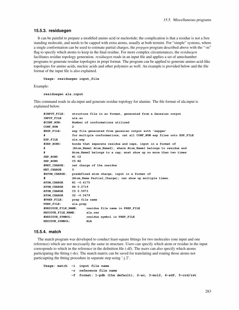
15.5. Miscellaneous programs
15.5.3. residuegen
It can be painful to prepare a modified amino acid or nucleotide; the complication is that a residue is not a freestanding molecule, and needs to be capped with extra atoms, usually at both termini. For “simple” systems, wherea single conformation can be used to estimate partial charges, the prepgen program described above with the “-m”flag to specify which atoms to keep in the final residue. For more complex circumstances, the residuegenfacilitates residue topology generation. residuegen reads in an input file and applies a set of antechamberprograms to generate residue topologies in prepi format. The program can be applied to generate amino-acid-liketopologies for amino acids, nucleic acids and other polymers as well. An example is provided below and the fileformat of the input file is also explained.
Usage: residuegen input_file
Example:
residuegen ala.input
This command reads in ala.input and generate residue topology for alanine. The file format of ala.input isexplained below.
#INPUT_FILE: structure file in ac format, generated from a Gaussian output
INPUT_FILE ala.ac
#CONF_NUM: Number of conformations utilized
CONF_NUM 2
#ESP_FILE: esp file generated from gaussian output with ’espgen’
# for multiple conformations, cat all CONF_NUM esp files onto ESP_FILE
ESP_FILE ala.esp
#SEP_BOND: bonds that separate residue and caps, input in a format of
# (Atom_Name1 Atom_Name2), where Atom_Name1 belongs to residue and
# Atom_Name2 belongs to a cap; must show up no more than two times
SEP_BOND N1 C2
SEP_BOND C5 N2
#NET_CHARGE: net charge of the residue
NET_CHARGE 0
#ATOM_CHARGE: predefined atom charge, input in a format of
# (Atom_Name Partial_Charge); can show up multiple times.
ATOM_CHARGE N1 -0.4175
ATOM_CHARGE H4 0.2719
ATOM_CHARGE C5 0.5973
ATOM_CHARGE O2 -0.5679
#PREP_FILE: prep file name
PREP_FILE: ala.prep
#RESIDUE_FILE_NAME: residue file name in PREP_FILE
RESIDUE_FILE_NAME: ala.res
#RESIDUE_SYMBOL: residue symbol in PREP_FILE
RESIDUE_SYMBOL: ALA
15.5.4. match
The match program was developed to conduct least-square fittings for two molecules (one input and onereference) which are not necessarily the same in structure. Users can specify which atom or residue in the inputcorresponds to which in the reference in the definition file (-df). The users can also specify which atomsparticipating the fitting (-ds). The match matrix can be saved for translating and roating those atoms notparticiapting the fitting procedure in separate step using ’-j 2’.
Usage: match -i input file name
-r reference file name
-f format: 1-pdb (the default), 2-ac, 3-mol2, 4-sdf, 5-crd/rst
283

15. Antechamber and GAFF
-o output file name
-l run log file name, default is "match.log"
-s selection mode
0: use all atoms (the default)
1: specify atom names
2: use atom defination file
3: use residue defination file - original residue IDs
4: use residue defination file - renumbered residue IDs
-ds definition string if selection modes of ’1’ or ’3’ or ’4’
e.g. ’C,N,O,CA’, or ’HET’ which stands for heavy atoms for ’-ds 1’)
-df definition file if selection mode of ’2’ or ’3’ or ’4’
records take a form of ’ATOM atom_id_input atom_id_reference’
or ’RES res_id_input res_id_reference’
-n number of atoms participating ls-fitting,
default is -1, which implies to use all the selected atoms
-m matrix file, default is "match.matrix"
-t job type:
0: calculate rms only, need -i and -r
1: lsfit, need -i, -r and -o the default
2: translation/rotation, need -i, -o and -m
Example:
match -f pdb -r 1be9.pdb -i 3pdz.pdb -o 3pdz_aligned.pdb -s 4 -ds "CA,C,N,O" -df 3pdz_1be9.corr
The program runs least-square fitting for the non-hydrogen main chain atoms of residues defined in the3pdz_1be9.corr. A part of the 3pdz_1be9.corr is shown below:
RES 34 35 G GRES 35 36 I IRES 36 37 Y F...RES 87 88 L IRES 88 89 L I
15.5.5. match_atomname
One limitation of the Antechamber package is that the atom name information is lost after running Gaussiancalculations. And a residue topology file in prepi or prepc or a mol2 file generated from the Gaussian output hasatom names not matching those from the original file (usually a pdb file). Because of this glitch, one can notsimply load the residue topology file to tleap, read in the pdb file and then to save the topolgoy. We developedmatch_atomname to address this problem. The match_atomname program takes an input file and a reference filein pdb, ac, prepi, prepc and mol2 format, automatically detects the corresponding atom name in the reference foreach atom name in the input. An output file in the same format as that of the input is generated using the matchedatom names.
Usage: match_atomname -i input file name
-fi input format (pdb, ac, prepi, prepc, mol2
-r ref file name
-fr ref format (pdb, ac, prepi, prepc, mol2)
-o output file name
-h include hydrogen atoms or not
0 not, the default
1 yes
284

15.6. New Development of Antechamber And GAFF
-g geometric info (such as E/Z configuration) is considered to describe chemical enviornment
0 no, the default
1 yes
-l maximum path length, default is -1 (full length)
if it takes very long time and/or core dump occur, a value between 8 to 10 is recommended
Example:
match_atomname -i SAH.prepi -fi prepi -o SAH_matched.prepi -r SAH_XRAY.pdb -fr pdb
The output, SAH_matched.prepi and SAH_XRAY.pdb can be loaded to tleap directly to generate a topology forminimization or MD simulations.
15.6. New Development of Antechamber And GAFF
One important of functions of Antechamber is to assign AM1-BCC charges for organic molecules. Openeye’sQuacpak module can also assign AM1-BCC charges. The careful users may find that the charges assigned by thetwo programs are only marginally different (the largest charge difference is smaller than 0.05) in most cases. Thedifference is probably rooted from the difference of AM1 Mulliken charges. In unusual cases, large discrepancyoccurs (the largest charge difference is larger than 0.1). Recently, we have systematically studied 585 marketeddrugs using the both packages and the result is presented below. As the general AMBER force field is tightlyrelated to the antechamber package, the new development of the GAFF is also summarized here.
15.6.1. Extensive Test of AM1-BCC Charges
Three methods, namely Antechamber/Mopac (Mulliken charges are calculated by Mopac), Antechamber/Sqm(Mulliken charges are calculated by sqm) and Openeye’s Quacpak have been applied to assign the AM1-BCCcharges for the 585 drug molecules. The first two methods give essentially similar charges for all the cases andthe average charge difference is 0.005. The Quacpak, on the other hand, has an average charge difference of0.015 to Antechamber/Mopac. When compared to RESP charges, the average charge differences are 0.102 and0.105 for Antechamber/Mopac and Quacpak, respectively. In AM1-BCC, five BCC parameters were adjusted inorder to improve agreement with the experimental free energies of solvation. Adjustments were made to bonds ofamine nitrogen-H and amine nitrogen-tetravalent carbon.[318, 319] As a consequence, the average largest chargedifferences between AM1-BCC and RESP charges are very big: 0.441 for Antechamber/Mopac and 0.452 forQuacpak.
There are 71 molecules (12%) having the largest charge difference larger than 0.1 between Antechamber/Mopacand Quacpak. In comparison with the RESP charges, the average charge differences of the 71 molecules are 0.107and 0.129 for Antechamber/Mopac and Quacpack, respectively. As to the average largest charge differences, thecorresponding values are 0.444 and 0.522. It is clearly that Antechamber/Mopac-bcc has a similar average chargedifferences to RESP for the whole data set and the 71-molecule subset (0.102 vs 0.107), in contrast, Quacpac hasa much larger average charge difference for the 71 molecules (0.129) than that of the whole data set (0.105). Thesimilar trend is observed for the average largest charge difference as well (0.441 vs 0.444 for Antechamber/Mopacand 0.452 vs 0.522 for Quacpac).
15.6.2. New Development of GAFF
We have modified some parameters according to users’ feedback. We would like to thank users who provideus nice feedback/suggestion, especially David Mobley and Gabriel Rocklin. This version (GAFF1.4) is a meta-version between gaff1.0 and gaff2.0 and the following is the major changes:
1. All the sp2 carbon in a AR2 ring (such as pyrrole, furan, pyrazole) are either ’cc’ or ’cd’ atom types (not’c2’ any more). This is suggested by Gabriel Rocklin from UCSF. This modification improves the planarityof multiple-ring systems
285

15. Antechamber and GAFF
2. New van der Waals parameters have been developed for ’br’ and ’i’ atom types. The current parameters canwell reproduce the experimental density data of CH3Br (1.6755, 20 degree) and CH3I (2.2789, 20 degree):1.642 for CH3Br and 2.25 for CH3I, in contrast, the old parameters give 1.31 and 1.84, respectively.[325]
3. New van der Waals parameters have been suggested by David Mobley for ’c1’, ’cg’ and ’ch’ atom types.[326]
4. We have performed B3LYP/6-31G* optimization for 15 thousands marketed or experimental drugs/bio-actives. Reliable bond length and bond angle equilibrium parameters were obtained by statistics: each bondlength parameter must show up at least five times and has a rmsd smaller than 0.02 Å; each bond angleparameter must show up at least five times and has a rmsd smaller than 2.5 degrees. Those new parametersnot showing up in old gaff were directly added into gaff 1.4; and some low-quality gaff parameters whichshow up less than five times or have large rmsd values (>0.02 Å for bond length and >5 degrees for bondangles) were replaced with those newly generated. In summary, 59 low quality bond stretching parameterswere replaced and 56 new parameters were introduced; 437 low quality bond bending parameters werereplaced and 618 new parameters were introduced.
15.7. Metal Center Parameter Builder (MCPB)
15.7.1. Introduction
The Metal Center Parameter Builder (MCPB) program provides a means to rapidly build, prototype, and validateMM models of metalloproteins. It uses the bonded plus electrostatics model to expand existing pairwise additiveforce fields. It was developed by Martin Peters at the University of Florida in the lab of Kenneth Merz Jr. MCPBis described fully Ref. [317].
Why is it desirable to model metalloprotein systems using MM models and more precisely within the bondedplus electrostatic model? Structure/function and dynamics questions that are not currently attainable using QMor QM/MM based methods due to unavailability of parameters or system size can be answered. Force fields havebeen developed for zinc, copper, nickel, iron and platinum containing systems using the bonded plus electrostaticsmodel.
Incorporating metals into protein force fields can seem a daunting task due to the plethora of QM Hamiltonians,basis sets and charge models to choose from which the parameters are created. It was also generally carried outby hand without extensive validation for specific metalloproteins. MCPB was developed to remove the latter andcreate a framework in which to test various methods, basis sets and charges models in the creation of metalloproteinforce fields.
The MCPB program was built using the MTK++ Application Program Interface (API). For more informationregarding MTK++ and MCPB please see the MTK++ manual: $AMBERHOME/doc/MTKpp.pdf A more extensivedescription of metalloproteins and the theory within MCPB can be found in sections 10 to 12 of the MTK++manual.
15.7.2. Running MCPB
MCPB takes two command-line arguments. One is the control file, which is required and chosen with the -iflag. The other is the log file, which is optional and chosen with the -l flag. A full listing of all the commands usedby MCPB can be obtained with the -f flag.
MCPB: Semi-automated tool for metalloprotein parametrization
usage: MCPB [flags] [options]
options:
-i script file
-l log file
flags:
-h help
-f function list
286

15.8. Python Metal Site Modeling Toolbox (pyMSMT)
Full details of a metalloprotein parametrization procedure using MCPB can be found in section 15.10 of theMTK++ manual. This example describes the active site parametrization of a di-zinc system (PDB ID: 1AMP).The parametrization is broken down into stages since several MCPB operations rely on the output of externalpackages such as Gaussian and RESP. Most of the steps are carried out using MCPB but some require user inputand instruction.
15.8. Python Metal Site Modeling Toolbox (pyMSMT)
15.8.1. Introduction
The Python Metal Site Modeling Toolbox (pyMSMT) is a python package for metal site modeling of mixedsystems (especially protein systems) for ultimate use in molecular dynamics simulations. It could facilitate param-eterizaiton of both the bonded and nonbonded models. This toolbox was developed by Pengfei Li in Prof. KennethM. Merz, Jr.’s research group at Michigan State University. Users are welcome to send suggestions and bug reportsto AMBER Mailing List ([email protected]).
In the current version, six applications are supported by the pyMSMT package:1) MCPB.py: a Python version for the Metal Center Parameter Builder (MCPB). MCPB.py supports various
metal ions (more than 80 metal ions with partial charges/oxidation-states from +1 to +8, literally), different AM-BER force fields (ff94, ff99, ff99SB, ff03, ff03.r1, ff10, ff14ipq, ff14SB, ff14SB.redq, ff14SBonlysc, ff15ipq,ff15ipq-vac, fb15, GAFF, and GAFF2 in the current version), different parameterization methods (Seminario,Z-matrix and empirical), and different models (bonded model and nonbonded models for metal ions). It couldfacilitate parameterization of both metalloproteins and organometallic compounds. The workflow is more efficientand many of the modeling processes in previous MCPB versions are automatically implemented into MCPB.py(MCPB.py uses about 10 fewer steps and many fewer scripts than MCPB). An application note of the program ispublished by Li and Merz.[327] The main scheme and parameters are based on previous papers published by Merzet al.[90–93, 317]
2) IPMach.py: the Python ion parameterization machine. IPMach.py could largely facilitate the parameterizationfor the 12-6 LJ model and 12-6-4 LJ-type model of ions. It could automatically parameterize the 12-6 LJ modelfor a given hydration free energy or ion-oxygen distance, and the 12-6-4 LJ-type model for given hydration freeenergy and ion-oxygen distance. This code in AmberTools16 package now is in its beta-version.
3) PdbSearcher.py: the Python version of Pdbsearcher. PdbSearcher.py better supports the automatic recognitionof the metal centers in a PDB file due to better compatibility with the PDB naming scheme of metal ions.
4) OptC4.py: a program to optimize theC4 terms of the 12-6-4 potential using the AMBER topology and co-ordinate files. It can automatically optimize the metal-site-relatedC4 terms to better reproduce the experimentalstructure. It uses the sum of unsigned error of metal site bond lengths, angles and dihedrals as the criterion (inwhich the bond, angle and dihedral have different weights). For each optimization cycle, the structure will be min-imized by OpenMM[328, 329] and then have the sum of unsigned error calculated. It requires OpenMM version6.3 and an installed SciPy package in current version.
5) CartHess2FC.py: the program to calculate the force constants using Cartesian Hessian matrix based on Sem-inario method. It could calculate all the bond and angle force constants of a system based on a Gaussian fchk fileor GAMESS log file which containing the Cartesian Hessian matrix.
6) espgen.py: the Python version of espgen in the antechamber package. It could extract the electrostatic poten-tial information from a Gaussian output file or GAMESS log file which containing these information. It supportsGaussian03, Gaussian09 and GAMESS.
15.8.2. Usage
The following is a summary of the usage and options for the three applications:
15.8.2.1. MCPB.py
Usage: MCPB.py -i input_file -s/--step step_number
[--logf Gaussian/GAMESS-US output logfile]
287

15. Antechamber and GAFF
[--fchk Gaussian fchk file]
Options:
-h, --help Show this help message and exit
-i INPUTFILE Input file name
-s STEP, --step=STEP Step number
--logf Gaussian/GAMESS-US output logfile
--fchk Gaussian fchk file
The following is an introduction of the variables in the input_file:(Reminder: there should be no blank lines in the input_file. The values or parameters should follow the variables
separated by a space.)Required variables:
ion_ids The PDB atom ID of the complex’s central metal ion. It should be an integer value, depending on howmany metal ions are included in the metal complex.
ion_info This variable is only required for the nonbonded model without refitting the residue charges (step number4n2). In all, there are four data points required for each metal ion: 1) the residue name of the metal ion inthe PDB file; 2) the atom name of the metal ion in the PDB file; 3) the element symbol of the metal ion; 4)the charge (or oxidation state, which needs to be an integer) of the metal ion. For example: ZN ZN Zn 2 (thefirst two are the residue and atom name of the Zn2+ ion in the PDB file, the third is its element symbol andthe last one is its charge).
ion_mol2files The name(s) of the ion(s) in the mol2 file(s) contained in the metal center. This can be one orseveral name(s), depending on how many kinds of ions are included in the metal center. The user can useantechamber to transfer the single ion PDB file to a mol2 file and then manually modify the atom type andthe atomic charge of the metal ion in the mol2 file.
original_pdb This is the file name of the original PDB file, which should have only one chain. The PDB fileshould have hydrogen atoms and metal ions in it. Users are advised to use an application like pdb4amber toclean up the PDB file first. They are also advised to add the hydrogen atoms by using a webserver such asH++ before performing the modeling in MCPB.py.
Optional variables:
add_bonded_pairs Specify the bonded atom pair(s) you want to add in the model building by MCPB.py. Indefault MCPB.py only detect the Metal-N/O/S/F/Cl/Br/I bond, if you have a other kind of metal ligatingbond in the metal site (e.g. Metal-C bond), you need to specify the atom numbers of metal and the ligatingatom in the input file. There should be even numbers after the variable with space seperate. For example,if you have two Metal-C bond in the metal site, and the metal has atomic number as 1001, while the twocarbon atoms have atomic numbers as 1320 and 1380 respectively, you can use add following line in theinput file: "add_bonded_pairs 1001 1320 1001 1380". [The default value of this variable is the null list.]
additional_resids Specify the residues’ IDs for which you want to add to the models built by MCPB.py. Forexample, it may be a residue in the second layer which coordinates a metal bonded residue. It will increasethe computational cost for QM calculations. [The default value of this variable is the null list.]
anglefc_avg A variable used to indicate whether to make an average of angle force constants derived based ondifferent manners of chosing the sub-matrices in Seminario method. There are A-B and B-A two ways ofchosing the sub-matrix for two atoms in the parameter derivation process based on Seminario method. Theangle force constant obtained based on different manners of chosing the sub-matrices may not have bigdifferences. Two options are aviable: 0 or 1. 0 means not making average, using the default manner to chosethe sub-matrices. 1 means making average of different manners to chose the sub-matrices. [The default is0.]
288

15.8. Python Metal Site Modeling Toolbox (pyMSMT)
bondfc_avg A variable used to indicate whether to make an average of bond force constants derived based ondifferent manners of chosing the sub-matrix in Seminario method. There are A-B and B-A two ways ofchosing the sub-matrix for two atoms in the parameter derivation process based on Seminario method. Thebond force constant obtained based on different manners of chosing the sub-matrix would not have bigdifferences. Two options are aviable: 0 or 1. 0 means not making average, using the default manner to chosethe sub-matrix. 1 means making average of different manners to chose the sub-matrix. [The default is 0.]
chgfix_resids Specify the residues’ IDs whose charges are going to be fixed during the charge fitting. The fixedcharge values are referenced from the mol2 files used during the modeling. [The default value of this variableis the null list.]
cut_off The cutoff value is used to indicate there is a bond between the metal ion and the surrounding atoms. Theunit is Angstroms. [The default is 2.8.]
force_field The user-designated name of the force field. The current version supports ff94, ff99, ff99SB, ff03,ff03.r1, ff10, ff14ipq, ff14SB, ff14SB.redq, ff14SBonlysc, ff15ipq, ff15ipq-vac, and fb15. [The default isff14SB.]
frcmod_files The variable used to indicate the parameter modification file(s) for the nonstandard residue(s) (e.g.frcmod file generated by parmchk for a ligand molecule) in the metal complex. It can be one name or severalnames seperated by space. [The default value of this variable is the null list.]
gaff A variable used to indicate the use of a GAFF force field during the modeling. 0 means no, 1 means usingGAFF, 2 means using GAFF2. [The default is 1.]
group_name The group name the user has specified. The group name is the prefix for different kinds of modelingfiles e.g. PDB, fingerprint and Gaussian input files for different models. [The default is MOL.]
ion_paraset The user-designated ion parameter set to be used in the nonbonded model. (This option has noinfluence on the metal ion VDW parameters in the bonded model, in which the author has chosen certainVDW parameter sets for different ions.) There are four options for this variable: HFE, CM, IOD and 12_6_4(reminder: there are underlines between the numbers). If you use the 12-6 Lennard-Jones nonbonded model,the recommended settings are the HFE set for the +1 and -1 ions, the CM set for the +2 ions, and the IODset for the +3 and +4 ions. They are also the default settings for these metal ions.
large_opt A variable used to indicate whether to do an geometry optimization in the Gaussian input file. Threeoptions are aviable: 0, 1, or 2. 0 means no optimization, 1 means only optimizing the hydrogen positions, 2means full geometry optimization. [The default is 0.]
lgmodel_chg Specify the total charge of the large model. [The default value of the charge will be assignedautomatically by the program, which is not guaranteed to be right. Careful check is suggested from runnningthe Gaussian/GAMESS-US program. If it is not right, you can add this option with right charge into the inputfile and regenerate the modeling files.]
naa_mol2files The variable used to indicate non-amino acid mol2 file(s) in the metal complex if there are anynonstandard residue(s) in the metal complex. Examples of nonstandard residues include hydroxyl group andligand molecules. For these residues, the user can use antechamber to generate the mol2 file(s) by first doingan AM1-BCC or HF/6-31G* RESP charge fit and then assigning an AMBER atom type (recommended forwater or hydroxyl group) or a GAFF atom type (recommended for ligand). [The default value of this variableis the null list.]
scale_factor Specify the frequency scale factor for force constant derivation based on QM methods. This scalefactor will scale all the bond and angle force constants determined from the QM calculations.Reminder: Theforce constant scale factor is usually equals the sqaure of frequency scale factor. For example, if you areusing HF/6-31G* level of theory to do calculation and its frequency scale factor is 0.9, the force constantscale factor you need to use is 0.9^2=0.81. [The default value is 1.0 (no scaling performed).]
289
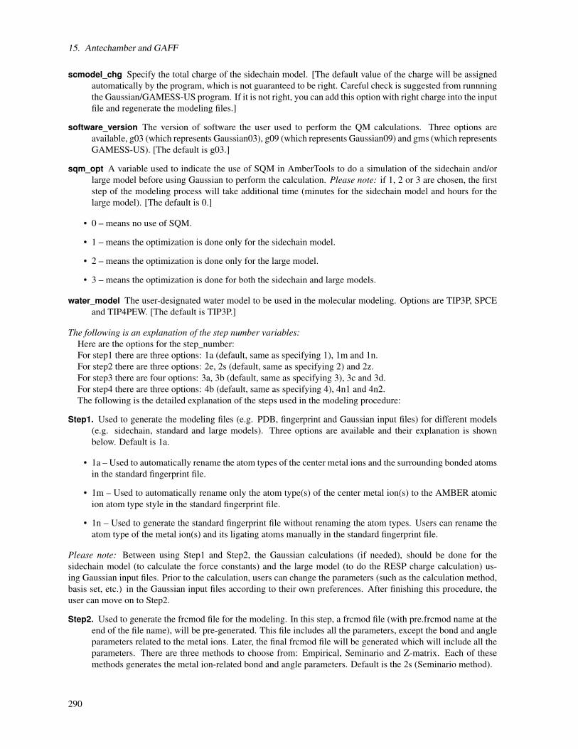
15. Antechamber and GAFF
scmodel_chg Specify the total charge of the sidechain model. [The default value of the charge will be assignedautomatically by the program, which is not guaranteed to be right. Careful check is suggested from runnningthe Gaussian/GAMESS-US program. If it is not right, you can add this option with right charge into the inputfile and regenerate the modeling files.]
software_version The version of software the user used to perform the QM calculations. Three options areavailable, g03 (which represents Gaussian03), g09 (which represents Gaussian09) and gms (which representsGAMESS-US). [The default is g03.]
sqm_opt A variable used to indicate the use of SQM in AmberTools to do a simulation of the sidechain and/orlarge model before using Gaussian to perform the calculation. Please note: if 1, 2 or 3 are chosen, the firststep of the modeling process will take additional time (minutes for the sidechain model and hours for thelarge model). [The default is 0.]
• 0 – means no use of SQM.
• 1 – means the optimization is done only for the sidechain model.
• 2 – means the optimization is done only for the large model.
• 3 – means the optimization is done for both the sidechain and large models.
water_model The user-designated water model to be used in the molecular modeling. Options are TIP3P, SPCEand TIP4PEW. [The default is TIP3P.]
The following is an explanation of the step number variables:Here are the options for the step_number:For step1 there are three options: 1a (default, same as specifying 1), 1m and 1n.For step2 there are three options: 2e, 2s (default, same as specifying 2) and 2z.For step3 there are four options: 3a, 3b (default, same as specifying 3), 3c and 3d.For step4 there are three options: 4b (default, same as specifying 4), 4n1 and 4n2.The following is the detailed explanation of the steps used in the modeling procedure:
Step1. Used to generate the modeling files (e.g. PDB, fingerprint and Gaussian input files) for different models(e.g. sidechain, standard and large models). Three options are available and their explanation is shownbelow. Default is 1a.
• 1a – Used to automatically rename the atom types of the center metal ions and the surrounding bonded atomsin the standard fingerprint file.
• 1m – Used to automatically rename only the atom type(s) of the center metal ion(s) to the AMBER atomicion atom type style in the standard fingerprint file.
• 1n – Used to generate the standard fingerprint file without renaming the atom types. Users can rename theatom type of the metal ion(s) and its ligating atoms manually in the standard fingerprint file.
Please note: Between using Step1 and Step2, the Gaussian calculations (if needed), should be done for thesidechain model (to calculate the force constants) and the large model (to do the RESP charge calculation) us-ing Gaussian input files. Prior to the calculation, users can change the parameters (such as the calculation method,basis set, etc.) in the Gaussian input files according to their own preferences. After finishing this procedure, theuser can move on to Step2.
Step2. Used to generate the frcmod file for the modeling. In this step, a frcmod file (with pre.frcmod name at theend of the file name), will be pre-generated. This file includes all the parameters, except the bond and angleparameters related to the metal ions. Later, the final frcmod file will be generated which will include all theparameters. There are three methods to choose from: Empirical, Seminario and Z-matrix. Each of thesemethods generates the metal ion-related bond and angle parameters. Default is the 2s (Seminario method).
290

15.8. Python Metal Site Modeling Toolbox (pyMSMT)
• 2e – The Empirical method,[330]can generate the metal ion-related bond and angle parameters efficientlywithout doing Gaussian calculations. It only supports Zn2+ ion in the current version.
• 2s – The Seminario method[331] generates the force field parameters based on sub-matrices of the CartesianHessian matrix obtained from quantum calculations. This method requires a Gaussian fchk file (which canbe generated from a chk file by using the formchk command in Gaussian).Reminder: both the geometry op-timization and force constant calculation procedures are needed to generate the final chk file and subsequentfchk file for the force constant calculations done by the Seminario method.
• 2z – The Z-matrix method generates the force field parameters by using the Cartesian Hessian matrix ob-tained from the quantum calculations. This method requires the force constant Gaussian output file (usuallynamed as a log file) after the geometry optimization and force constant calculations.
Step3. Used to perform the RESP charge fitting and to generate the mol2 files for the residues within the metalion complex. There are several fitting schemes available in this step. The four options are shown below.The default is 3b since Seminario/ChgModB was identified as the best combination in the work of Peterset al.[317]Reminder: the chgfix_resids variable is effective in this procedure, if the variable is specified, thecharge restriction will be used as well as one of the following choices.
• 3a – Allows all the charges of the atoms in the ligating residues to change without any restrictions.
• 3b – Restrains the charges of the heavy backbone atoms in the ligating residues according to the user-chosenforce field.
• 3c – Restrains the charges of the backbone atoms (both heavy and hydrogen atoms) in the ligating residuesaccording to the user-chosenforce field.
• 3d – Restrains the charges of the backbone atoms (both heavy and hydrogen atoms) and C beta atoms in theligating residues according to the user-chosen force field.
Step4. Generates the leap input file. The default is 4b.
• 4b – Generates the leap input file for the bonded model.
• 4n1 – Generates the leap input file for the nonbonded model and refits the charge of the ligating residues.
• 4n2 – Generates the leap input file for the nonbonded model without refitting the charge of the ligatingresidues.
Here are some suggestions for the parameterization procedure:1) For the modeling of the bonded model, the following steps are usually needed (4 steps):
1a/1n→2e/2s/2z→3a/3b/3c/3d→4b2) For the modeling of a non-bonded model with a refitted charge, users can follow the workflow (3 steps):
1m→3a/3b/3c/3d→4n13) For modeling with a normal nonbonded model (without fitting any charges), users usually only need one step
to perform the modeling (1 step): 4n2.The following is an explanation of the logf and fchk variables:These variables are optional. If provided, they are only active in step2 and/or step3. The default log file name
is group_name + ’_sidechain_fc.log’ for step2 and group_name + ’_large_mk.log’ for step3. The default fchk filename is group_name + ’_sidechain_opt.fchk’ and it is only active for step2 when using Gaussian software andSeminario method to obtain the force constant parameters.
If you are using Gaussian software and Seminario method to generate force constant parameters, it uses the fchkfile of sidechain model to store the Cartesian Hessian matrix. If you are using Gaussian software and Z-matrixmethod to generate force constant parameters, it uses the log file of sidechain model to store the force constantparameters. While if you are using GAMESS-US software and Seminario method to generate the force constants,it uses the log file of sidechain model to store the Cartesian Hessian matrix. In current version the software doesn’tsupport GAMESS-US with Z-matrix method to generate the force constants.
Both the Gaussian and GAMESS-US software use the log file of large model to store the ESP charges.
291
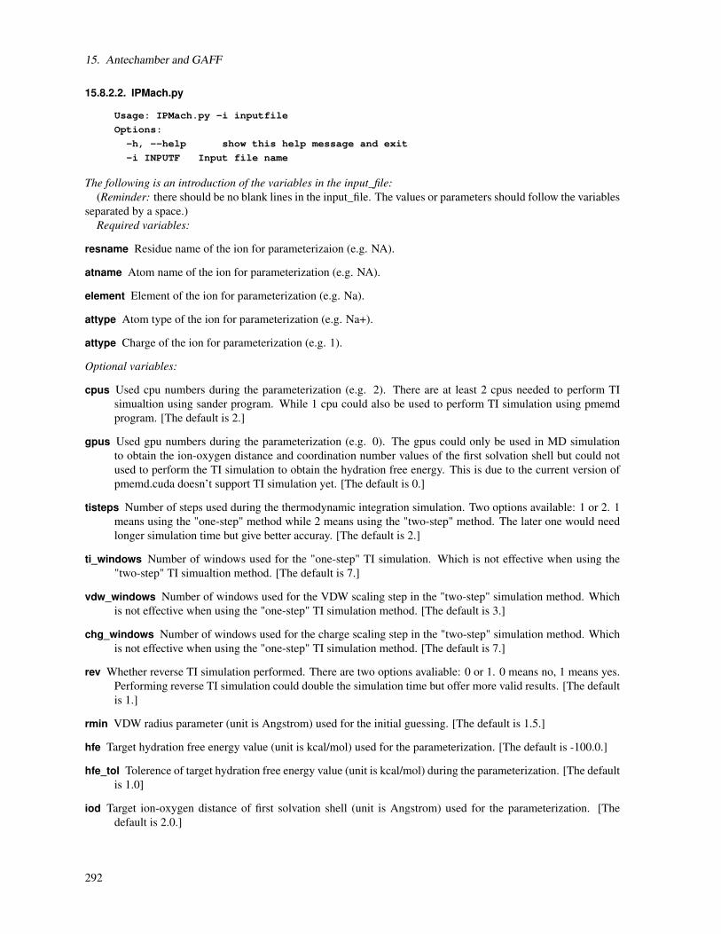
15. Antechamber and GAFF
15.8.2.2. IPMach.py
Usage: IPMach.py -i inputfile
Options:
-h, --help show this help message and exit
-i INPUTF Input file name
The following is an introduction of the variables in the input_file:(Reminder: there should be no blank lines in the input_file. The values or parameters should follow the variables
separated by a space.)Required variables:
resname Residue name of the ion for parameterizaion (e.g. NA).
atname Atom name of the ion for parameterization (e.g. NA).
element Element of the ion for parameterization (e.g. Na).
attype Atom type of the ion for parameterization (e.g. Na+).
attype Charge of the ion for parameterization (e.g. 1).
Optional variables:
cpus Used cpu numbers during the parameterization (e.g. 2). There are at least 2 cpus needed to perform TIsimualtion using sander program. While 1 cpu could also be used to perform TI simulation using pmemdprogram. [The default is 2.]
gpus Used gpu numbers during the parameterization (e.g. 0). The gpus could only be used in MD simulationto obtain the ion-oxygen distance and coordination number values of the first solvation shell but could notused to perform the TI simulation to obtain the hydration free energy. This is due to the current version ofpmemd.cuda doesn’t support TI simulation yet. [The default is 0.]
tisteps Number of steps used during the thermodynamic integration simulation. Two options available: 1 or 2. 1means using the "one-step" method while 2 means using the "two-step" method. The later one would needlonger simulation time but give better accuray. [The default is 2.]
ti_windows Number of windows used for the "one-step" TI simulation. Which is not effective when using the"two-step" TI simualtion method. [The default is 7.]
vdw_windows Number of windows used for the VDW scaling step in the "two-step" simulation method. Whichis not effective when using the "one-step" TI simulation method. [The default is 3.]
chg_windows Number of windows used for the charge scaling step in the "two-step" simulation method. Whichis not effective when using the "one-step" TI simulation method. [The default is 7.]
rev Whether reverse TI simulation performed. There are two options avaliable: 0 or 1. 0 means no, 1 means yes.Performing reverse TI simulation could double the simulation time but offer more valid results. [The defaultis 1.]
rmin VDW radius parameter (unit is Angstrom) used for the initial guessing. [The default is 1.5.]
hfe Target hydration free energy value (unit is kcal/mol) used for the parameterization. [The default is -100.0.]
hfe_tol Tolerence of target hydration free energy value (unit is kcal/mol) during the parameterization. [The defaultis 1.0]
iod Target ion-oxygen distance of first solvation shell (unit is Angstrom) used for the parameterization. [Thedefault is 2.0.]
292

15.8. Python Metal Site Modeling Toolbox (pyMSMT)
iod_tol Tolerence of target ion-oxygen distance of first solvation shell (unit is Angstrom) during the parameteri-zation. [The default is 0.01.]
cal_type Type of the calculation: whether it is a optimization (OPT), or single point calculation (SP). [The defaultis OPT.]
set Parameter set to generate. There are two parameter set avaliable: HFE or IOD. The HFE parameter set willtreat hydration free energy as target during the parameterization. The IOD parameter set will treat ion-oxygen distance of first solvation shell as target during the parameterization. [The default is HFE.]
maxiter Maxium iteriation steps during the parameter optimization. [The default is 100.]
mode There are three modes avaliable for running the program: test, scan, normal. These three modes willincrease the simulation time one-by-one. [The default is normal]
program The MD program used during the parameterization. Two options: sander or pmemd. Reminder: pmemdcould not used to perform TI simulation for 12-6-4 LJ-type model. [The default is sander.]
watermodel Water model used during the parameterization. The ion parameters may vary for different watermodels. It is suggested to parameterize a ion model for a specific water model. Seven options: tip3p, tip4p,tip4pew, tip5p, spc, spce, and opc. [The default is tip3p.]
c4 Initial C4 values between ion and oxygen in water for parameterization of the 12-6-4 model for ions. Its unit iskcal/mol * Angstrom^4. [The default is 0, means only 12-6 parameters with no C4 parameters applied.]
15.8.2.3. PdbSearcher.py
Usage: PdbSearcher.py -i/--ion ionname -l/--list input_file
-e/--env environment_file -s/--sum summary_file
[-c/--cut cutoff]
Options:
-h, --help Show this help message and exit
-i IONNAME, --ion=IONNAME Element symbol of ion, e.g. Zn
-l INPUTF, --list=INPUTF List file name, list file contains one
PDB file name per line
-e ENVRMTF, --env=ENVRMTF Environment file name. An environment file is used
to store the metal center environment information
such as ligating atoms, distance, geometry etc.
For each bond, there is a record.
-s SUMF, --sum=SUMF Summary file name. A summary file is used to store
the metal center summary information such as metal
center geometry, ligating residues etc. For each
metal center there is a record.
-c CUTOFF, --cut=CUTOFF Optional. The cut off value used to detect the
bond between metal ion and ligating atoms.
The unit is Angstroms. If there is no value
specified, the default algorithm will be used.
The default algorithm recognizes the bond when
its distance is no less than 0.1 (smaller than 0.1
usually indicates a low quality structure) and no
bigger than the covalent radius sum of the two
atoms with a tolerance of 0.4.
293

15. Antechamber and GAFF
15.8.2.4. OptC4.py
Usage: OptC4.py -m amber_mask -p topology_file -c coordinate_file -r restart_file
[--maxsteps maxsteps] [--phase simulation_phase]
[--size optimization_step_size] [--method optimization_method]
[--platform device_platform] [--model metal_complex_model]
Options:
-h, --help Show this help message and exit
-m ION_MASK Amber mask of the center metal ion
-p PFILE Topology file
-c CFILE Coordinate file
-r RFILE Restart file
--maxsteps=MAXSTEPS Maximum minimization steps performed by OpenMM
in each parameter optimization cycle.
[Default: 1000]
--phase=SIMUPHA Simulation phase, either gas or liquid.
[Default: gas]
--size=STEPSIZE Step size chosen by the user for the C4 value
during parameter searching. [Default: 10.0]
--method=MINM Optimization method of the C4 terms, The options
are: powell, cg, bfgs or slsqp.[Default: bfgs]
Please check the website:
http://docs.scipy.org/doc/scipy/reference/optimize.html#module-scipy.optimize
for more information if interested.
--platform=PLATF Platform used. The options are: reference, cpu,
gpu or opencl. [Default: cpu] Here we use the
OpenMM software to perform the structure
minimization. Please check OpenMM user guide for
more information if interested.
--presn=PRESN Precision used. The options are: single, mixed, or
double. This option is only valid when using the CUDA
or OpenCL platform. [Default: single]
--model=MODEL The metal ion complex model chosen to calculate the sum
of unsigned average errors of bond lengths, angles, and
dihedrals (the units of them are angstrom, degree and
degree respectively while the weights of them are
1/100, 1/2 and 1 respectively). This sum is the
criterion for the optimization (with a smaller value,
the better the parameters). The options are: 1 or 2.
1 means a small model (only contains the metal ion
and binding heavy atoms) while 2 means a big model
(contains the metal ion and heavy atoms in the
ligating residues). [Default: 1]
15.8.2.5. CartHess2FC.py
Usage: CartHess2FC.py -p PDB_file -f QM_output_file [-v software] [-m method]
[--scalef freq_scale_factor] [--nstpdb]
[--bavg] [--avg13] [--aavg]
Options:
-h, --help show this help message and exit
-i INPUTFILE Input PDB file name
294
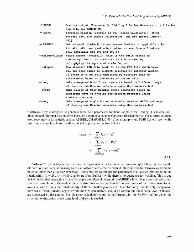
15.8. Python Metal Site Modeling Toolbox (pyMSMT)
-f HESSF Quantum output file name (a fchk/log file for Gaussian or a file for
log file for GAMESS-US).
-v SOFTV Software version [Default is g03 (means Gaussian03), other
options are, g09 (means Gaussian09), and gms (means GAMESS-
US)]
-m METHOD Method used. [Default is sem (means Seminario, appliable other
for g03, g09, and gms) other option is zmx (means Z-matrix,
only appliable for g03 and g09.)]
--scalef=SCALEF Scale factor (ATTENTION: This is the scale factor of
frequency. The force constants will be scaled by
multiplying the square of scale_factor).
--nstdpdb Non standard PDB file used. It is the PDB file which have
all the atom names as element followed by interger number.
It could be a PDB file generated by software such as
antechamber based on the Gaussian output file.
--bavg Make averge of bond force constants based on different ways
of chosing sub Hessian matrices using Seminario method.
--avg13 Make averge of Urey-Bradley force constants based on
different ways of chosing sub Hessian matrices using
Seminario method.
--aavg Make averge of angle force constants based on different ways
of chosing sub Hessian matrices using Seminario method.
CartHess2FF.py is designed to generate force field parameters for bond, angle, Urey-Bradley (1-3 interaction),dihedral, and improper torsion terms based on quantum calculated Cartesian Hessian matrix. These terms could beused seperately in force fields such as AMBER, CHARMM, CNS (Crystallography and NMR System), etc. whilelimits may be applicable for the dihedral and improper terms (see below).
Etotal = ∑bonds
kb(r− r0)2
+ ∑angles
kθ (θ −θ0)2
+ ∑dihedrals
kφ (φ −φ0)2
(15.1)
CartHess2FF.py could generate the force field parameters for the potential shown in Eq15.1 based on the log fileof force constant calculation using Gaussian software and Z-matrix method. Here the dihedral term uses a harmonicpotential other than a Fourier expansion. Users may try to transfer the parameters to a Fourier term based on therelationship: Vn = 2kφ/n2 (whileVn andn are from Eq14.1 ) while there is no guarantee for working. This is dueto 1-4 nonbonded interaction is usually coupled to dihedral potential in AMBER while it is not considered currentpotential formulation. Meanwhile, there is also other issues (such as the connectivities of the central two atoms)avaliable which limits the transferability of these dihedral parameters. Therefore only qualitatively comparisonbetween different dihedral angles (while the QM calculations should be carried out under same level of theory)are suggested by the author. The Gaussian calculation could be performed with iop(7/33=1), before which thestructural optimization at the same level of theory is needed.
295

15. Antechamber and GAFF
Etotal = ∑bonds
kb(r− r0)2
+ ∑Urey−Bradley
ku (u−u0)2
+ ∑angles
kθ (θ −θ0)2
+ ∑dihedrals
kφ (φ −φ0)2
+ ∑impropers
kAN(rAN− rAN,0)2
(15.2)
Moreover, CartHess2FF.py could generate the force field parameters for the potential shown in Eq15.2 basedon the Cartesian Hessian matrix obtained by using Gaussian or GAMESS-US. Comparing to Eq15.1 it has anadditional Urey-Bradley (1-3 harmonic interaction) term and a harmonic improper torsion term (instead of a Fourierterm). In the harmonic improper term A and N represent the central atom and its projection into the plane of theother three atoms in the improper torsion. Herein kAN , rAN , and rAN,0 represent the force constant, distance andequlibrium distance between A and N respectively. Similarly, parameters of the dihedral and improper torsionterms have limited transferabilty and are only suggested to be used for qualitatively comparison. A fchk file isneeded for Gaussian and it could be obtained by using "formchk" command to get it based on the chk file after theforce constant calculation (again, before which a structural optimization at the same level of theory is needed). Alog file is needed for GAMESS-US force constant calculation (same as Gaussian, a structural optimization at thesame level of theory is needed before the calculation).
15.8.2.6. espgen.py
Usage: espgen.py -i input_file -o output_file [-v software]
Options:
-h, --help show this help message and exit
-i INPUTFILE Input file name
-o OUTPUTFILE Output file name
-v SOFTVERSION Software version [Default is gau (means Gaussian),
other option is gms (means GAMESS-US)]
296

16. Setting up crystal simulations
David S. Cerutti
Simulations of biomolecular crystals are in principle no different than any of the simulations that AMBERdoes in periodic boundary conditions. However, the setup of these systems is not trivial and probably cannotbe accomplished with the LEaP software. Of principal importance are the construction of the solvent conditions(packing precise amounts of multiple solvent species into the simulation cell), and tailoring the unit cell dimensionsto accommodate the inherently periodic nature of the system. The LEaP software, designed to construct simulationsof molecules in solution, will overlay a pre-equilibrated solvent mask over the (biomolecular) solute, tile that maskthroughout the simulation cell, and then prune solvent residues which clash with the solute. The result of thisprocedure is a system which will likely contract under constant pressure dynamics as the pruning process has leftvacuum bubbles at the solute:solvent interface. Simulations of biomolecular crystals require that the simulation cellbegin at a size corresponding to the crystallographic unit cell, and deviate very little from that size over the courseof equilibration and onset of constant pressure dynamics. This demands a different strategy for placing solvent inthe simulation cell. Four programs in the AmberTools release are designed to accomplish this. An example of theiruse in given in a web-based tutorial at http://ambermd.org/tutorials/advanced/tutorial13/XtalTutor1.html .
For brevity, only basic descriptions of the programs are given in this manual. All of the programs may berun with command line input; the input options to each program may be listed by running each program with noarguments.
16.1. UnitCell
A macromolecular crystal contains many repeating unit cells which stack like blocks in three dimensional spacejust as simulation cells do in periodic boundary conditions. Each unit cell, in turn, may contain multiple symmetry-related clusters of atoms. A PDB file contains one set of coordinates for the irreducible unit of the crystal, the“asymmetric unit,” and also information about the crystal space group and unit cell dimensions. The UnitCell pro-gram reads PDB files, seeking the SMTRY records within the REMARKs to enumerate the rotation and translationoperations which may be applied to the coordinates given in the PDB file to reconstuct one complete unit cell.
16.2. PropPDB
Simulations in periodic boundary conditions require a minimum unit cell size: the simulation cell must be ableto enclose a sphere of at least the nonbonded direct space cutoff radius plus a small buffer region for nonbondedpairlist updates. Many biomolecular crystal unit cells come in “shoebox” dimensions that may have one very shortside; many unit cells are also not rectangular but triclinic, meaning that the size of the largest sphere they canenclose is further reduced. For these reasons, and perhaps to ensure that the rigid symmetry imposed by periodicboundary conditions does not create artifacts (crystallographic unit cells are equivalent when averaged over alltime and space, but are not necessarily identical at any given moment), it may be necessary to include multiple unitcells within the simulation cell. This is the purpose of the PropPDB program: to propagate a unit cell in one ormore directions so that the complete simulation cell meets minimum size requirements.
16.3. AddToBox
The AddToBox program handles placement of solvent within a crystal unit cell or supercell (as may be createdby PropPDB). As described in the introduction, the basic strategy is to place solvent such that added solvent
297

16. Setting up crystal simulations
molecules do not clash with biomolecule solutes, but may clash with one another initially. This compromise isnecessary because enough solvent must be added to the system to ensure that the correct unit cell dimensions aremaintained in the long run, but it is not acceptable to place solvent within the interior of a biomolecule where itmight not belong and never escape.
The AddToBox program takes a PDB file providing the coordinates of a complete biomolecular unit cell orsupercell (argument -c), the dimensions by which that supercell repeats in space (-X, -Y, -Z for the three boxedge lengths, and -al, -bt, and -gm for the three unit cell angles), a PDB file describing the solvent residue to add(argument -a), and the number of copies of that solvent molecule to add (argument -na). AddToBox inherentlyassumes that the biomolecular unit cell it is initially presented may contain some amount of solvent already, andaccording to the AMBER convention of listing macromolecular solute atoms first and solvent last assumes thatthe first -P atoms in the file are the protein (or biomolecule). AddToBox will then color a very fine grid “black” ifthe grid point is within a certain distance of a biomolecular atom (argument -RP) or other solvent atom (argument-RW); the grid is “white” otherwise (the grid is stored in binary for memory efficiency). AddToBox will the makea copy of the solvent residue and randomly rotate and translate it somewhere within the unit cell. If all atomsof the solvent residue land on “white” grid voxels, the solvent molecule will become part of the system and thegrid around the newly added solvent will be blacked out accordingly. If the solvent molecule cannot be placed,this process will be repeated until a million consecutive failures are encountered, at which point the program willterminate. If AddToBox has not placed the requested number of solvent molecules by the time it terminates, the -Voption can be used to order the program to recursively call itself with progressively smaller solvent buffer distancesuntil all the requested solvent can be placed. The output of the AddToBox program is another PDB named by the-o option.
Successful operation of AddToBox may take practice. If multiple solvent species are required, as is the casewith heterogenous crystallization solutions, AddToBox may be called repeatedly with each input molecular cellbeing the previous call’s output. When considering crystal solvation, the order of addition is important! It isrecommended that rare species, such as trace buffer reagents, be added first, with large -RW argument to ensure thatthey are dispersed throughout the available crystal void zones. Large solvent species such as MPD (an isohexanediol commonly used in crystallization conditions) or should be added second, and with a sufficiently large -RWargument that methyl groups and ring systems cannot become interlocked (which will likely lead to SHAKE /vlimit errors). Small and abundant species such as water should be added last, as they can go anywhere that spaceremains.
It is likely that the unobservable “void” regions between biomolecules in most crystals do not contain solventspecies in proportion to their abundance in the crystallization solution–the vast majority of these regions are withina few Ångstroms of some biomolecular surface, and different biomolecular functional groups will preferentiallyinteract with some types of solvent over others. Also, in many crystals some solvent molecules are observed; inmany of these, the amount of solvent observed is such that it would be impossible to pack other species into theunit cell in proportion to their abundances in the crystallization fluid. In these cases, we recommend estimatingthe amount of volume that must be filled with solvent apart from solvent which has already been observed in thecrystal, and filling this void with solvent in proportion to the composition of the crystallization fluid. For example,if a crystal were grown in a 1:1 mole-to-mole water/ethanol mixture, and the crystal coordinates as deposited in thePDB contained 500 water molecules and 3 ethanol molecules, we would use AddToBox to add water and ethanol ina 1:1 ratio until the system contained enough solvent to maintain the correct volume during equilibrium dynamicsat constant pressure.
Finally, it is difficult to estimate exactly how much solvent will be needed to maintain the correct equilibriumvolume; the advisable approach is simply to make an initial guess and script the setup so that, over multiple runs andreconstructions, the correct system composition can be found. We recommend matching the equilibrium unit cellvolume to within 0.3% to keep this simulation parameter within the error of most crystallographic measurements.While errors of 0.5-1% will show up quickly after constant pressure dynamics begin, a 10 to 20ns simulation maybe needed to ensure that the correct equilibrium volume has been achieved.
298

16.4. ChBox
16.4. ChBox
After the complex process of adding solvent, the LEaP program may be used to produce a topology and initialset of coordinates based on the PDB file produced by AddToBox. By using the SetBox command, LEaP will createa periodic system without adding any more solvent on its own. The only problem with using LEaP at this pointis that the program will fail to realize that the system does tile in three dimensions if only the box dimensions areset properly. If visualized, the output of UnitCell / PropPDB will likely look jagged, but the output of AddToBox,containing lots of added water, will make it obvious how parts of biomolecules jutting out one face of the box fitneatly into open spaces on an opposite face. The topology produced by LEaP needs no editing; only the last line ofthe coordinates does. This can be done manually, but the ChBox program automates the process, taking the samecoordinates supplied to AddToBox and grafting them into the input coordinates file.
299

17. Using the AMOEBA Force Field with AMBER
This section describes how to set up a system using the AMOEBA force field for use in the AMBER software.See Section ?? for instructions on running simulations using the Amoeba force field after performing the setupdescribed in the following sections.
One of the prerequisites for running simulations with the AMOEBA force field is that you must have the TIN-KER software suite installed (see http://dasher.wustl.edu/tinker/ for downloads and documentation). The restof these instructions will assume that you unpacked the TINKER source code into a directory defined by theTINKER_HOME environment variable.
17.1. Installing TINKER
Download the TINKER source code (e.g., tinker-6.3.3.tar.gz) and untar it. For the purposes of theseinstructions we will suppose that you are unpacking the source code in /home/myname. The installation steps areenumerated and described below.
1. Unpack the tinker source code, move to the source code directory, and set the TINKER_HOME environmentvariable
tar zxvf tinker-6.3.3.tar.gz
cd tinker
export TINKER_HOME=”‘pwd‘” # For sh, bash, zsh, ksh, etc.
setenv TINKER_HOME “‘pwd‘” # For csh, tcsh
2. Locate the appropriate set of compilation scripts for your platform and compiler. Compiling with gfortran ona Mac, for instance, the installation scripts are located in $TINKER_HOME/macosx/gfortran whereas theyare located in $TINKER_HOME/linux/intel to use the Intel compilers on a Linux system. These scripts willbe used in the next step.
3. The instructions in this step assume the use of gfortran on a Linux machine—you may need to modify someof these commands according to step 2 above. There are 3 steps for building the Tinker suite of programs;the source code is first compiled into objects, the objects are collected into a library, and the programs arecreated by linking the program objects with the Tinker library. The commands below perform these threesteps in order.
cd $TINKER_HOME/source
$TINKER_HOME/linux/gfortran/compile.make # Compiles source code
$TINKER_HOME/linux/gfortran/library.make # Creates libtinker.a library
$TINKER_HOME/linux/gfortran/link.make # Create TINKER programs
After executing these steps, all of the programs will have the suffix .x in the $TINKER_HOME/source direc-tory.
4. The next step is to move all of the binaries. The rename script will remove the “.x” suffix and move all ofthe programs into $TINKER_HOME/bin.
mkdir $TINKER_HOME/bin
$TINKER_HOME/linux/gfortran/rename.make
300

17.2. Preparing the system with TINKER
17.2. Preparing the system with TINKER
The following subsections will outline the steps needed to create an Amber topology defining the AMOEBApotential.
17.2.1. Convert PDB to XYZ
The first step (after installing TINKER) is to convert an input PDB file into a TINKER .xyz file. The proceduredescribed in Chapter 12 still applies to preparing PDB files for use with TINKER. You can also create a box ofsolvent in a PDB file (using, for example, tleap or packmol) if you wish to simulate an explicitly solvated system.If your PDB file is named 4LYT.pdb (for example), the following text demonstrates using the pdbxyz programfrom Tinker. The first step is to generate a Tinker keyword file with the same prefix (4LYT in this example) as thePDB file. The main purpose of the keyword file for our purposes is to define the parameter file to use.
[myname@machine]$ echo “parameters $TINKER_HOME/params/amoebapro13” > 4LYT.key
[myname@machine]$ $TINKER_HOME/bin/pdbxyz 4LYT
######################################################################
##########################################################################
### ###
### TINKER --- Software Tools for Molecular Design ###
## ##
## Version 6.3 February 2014 ##
## ##
## Copyright (c) Jay William Ponder 1990-2014 ##
### All Rights Reserved ###
### ###
##########################################################################
######################################################################
In this case, the input parameter database (in this example amoebapro13.prm), is defined inside$TINKER_HOME/params (but Fortran programs do not expand environment variables, so the whole path must betyped here). This program will generate two files, 4LYT.xyz and 4LYT.seq. The format of each of these files isdefined in the Tinker documentation, but the 4LYT.xyz file is the one that is needed for the next step.
TIP
If you plan on simulating an explicitly solvated system, an effective strategy is to use tleap to create the PDBfile with the solvent box. You can also have tleap save a topology and coordinate file using the Amber force fieldas well. This will cause tleap to write the box lengths (and angles) to the bottom of the coordinate file as the lastline. An example is shown below.
60.3196490 71.0908570 64.4813050 90.0000000 90.0000000 90.0000000
This line shows that the box sides are 60.3 × 71.1 × 64.5Å in an orthorhombic box. You can then add thefollowing keywords to the 4LYT.key file, which needs to be set for the step described in Subsection 17.2.3. Thetext that should be added to 4LYT.key is shown below
a-axis 60.32
b-axis 71.10
c-axis 64.49
17.2.2. Create the analout
The next step requires capturing the output of the analyze program in Tinker. The analyze program takes aTinker .xyz file and prints out details about the parameters. The following command will generate the analout file.
301

17. Using the AMOEBA Force Field with AMBER
$TINKER_HOME/bin/analyze 4LYT PC > 4LYT.analout
17.2.3. Create the prmtop
The next step is to use tinker_to_amber (built as part of AmberTools) to create the topology file. If you are usingperiodic boundary conditions, you may need to add the definition of at least the a-axis. This is described as a tipfollowing Subsection 17.2.1.
The tinker_to_amber program is run as shown below
tinker_to_amber -name 4LYT -title “4LYT Amoeba FF”
This step will generate the files 4LYT.prmtop and 4LYT.inpcrd. The information printed to the screen during theexecution of tinker_to_amber is diagnostic. It may be compared against the information printed to the topologyfile, but is not needed for running calculations. You should also check that the box information printed to the inpcrdfile matches what you expect. If you created a topology and inpcrd file using the Amber force field as described inthe tip following Subsection 17.2.1, you can match the information in the UNIT_CELL_PARAMETERS section of theinpcrd file with the last line of the Amber force field coordinate file.
302

Part IV.
Running simulations
303


18. sander
18.1. Introduction
This is a guide to sander, the Amber module which carries out energy minimization, molecular dynamics, andNMR refinements. The acronym stands for Simulated Annealing with NMR-Derived Energy Restraints, but thismodule is used for a variety of simulations that have nothing to do with NMR refinement. Some general featuresare outlined in the following paragraphs:
1. Sander provides direct support for several force fields for proteins and nucleic acids, and for several watermodels and other organic solvents. The basic force field implemented here has the following form, which isabout the simplest functional form that preserves the essential nature of molecules in condensed phases:
V (r) = ∑bonds
Kb(b−b0)2 + ∑
anglesKθ (θ −θo)
2
+ ∑dihedrals
(Vn/2)(1+ cos[nφ −δ ]
+ ∑nonbi j
(Ai j/r12i j )− (Bi j/r6
i j)+(qiq j/ri j)
"Non-additive" force fields based on atom-centered dipole polarizabilities can also be used. These add a"polarization" term to what was given above:
Epol =−2∑i
µi ·Eio
where µi is an induced atomic dipole. In addition, charges that are not centered on atoms, but are off-center(as for lone-pairs or "extra points") can be included in the force field.
2. The particle-mesh Ewald (PME) procedure (or, optionally, a "true" Ewald sum) is used to handle long-range electrostatic interactions. Long-range van der Waals interactions are estimated by a continuum model.Biomolecular simulations in the NVE ensemble (i.e. with Newtonian dynamics) conserve energy well overmulti-nanosecond runs without modification of the equations of motion.
3. Two periodic imaging geometries are included: rectangular parallelepiped and truncated octahedron (boxwith corners chopped off). (Sander itself can handle many other periodically-replicating boxes, but inputand output support in LEaP and ptraj is only available right now for these two.) The size of the repeating unitcan be coupled to a given external pressure, and velocities can be coupled to a given external temperatureby several schemes. The external conditions and coupling constants can be varied over time, so varioussimulated annealing protocols can be specified in a simple and flexible manner.
4. It is also possible to carry out non-periodic simulations in which aqueous solvation effects are representedimplicitly by a generalized Born/ surface area model by adding the following two terms to the "vacuum"potential function:
∆Gsol = ∑i j(1− 1
ε)(qiq j/ fGB(ri j)+A∑
iσi
305

18. sander
The first term accounts for the polar part of solvation (free) energy, designed to provide an approximationfor the reaction field potential, and the second represents the non-polar contribution which is taken to beproportional to the surface area of the molecule.
5. Users can define internal restraints on bonds, valence angles, and torsions, and the force constants and targetvalues for the restraints can vary during the simulation. The relative weights of various terms in the forcefield can be varied over time, allowing one to implement a variety of simulated annealing protocols in asingle run.
6. Internal restraints can be defined to be "time-averaged", that is, restraint forces are applied based on the aver-aged value of an internal coordinate over the course of the dynamics trajectory, not only on its current value.Alternatively, restraints can be "ensemble-averaged" using the locally-enhanced-sampling (LES) option.
7. Restraints can be directly defined in terms of NOESY intensities (calculated with a relaxation matrix tech-nique), residual dipolar couplings, scalar coupling constants and proton chemical shifts. There are provi-sions for handling overlapping peaks or ambiguous assignments. In conjunction with distance and angleconstraints, this provides a powerful and flexible approach to NMR structural refinements.
8. Replica exchange calculations can allow simultaneous sampling at a variety of conditions (such as tempera-ture), and allow the user to construct Boltzmann samples in ways that converge more quickly than standardMD simulations. Other variants of biased MD simulations can also be used to improve sampling.
9. Restraints can also be defined in terms of the root-mean-square coordinate distance from some referencestructure. This allows one to bias trajectories either towards or away from some target. Free energies can beestimated from non-equilibrium simulations based on targetting restraints.
10. Free energy calculations, using thermodynamic integration (TI) with a linear or non-linear mixing of the"unperturbed" and "perturbed" Hamiltonian, can be carried out. Alternatively, potentials of mean force canbe computed using umbrella sampling.
11. The empirical valence bond (EVB) scheme can be used to mix "diabatic" states into a potential that canrepresent many types of chemical reactions that take place in enzymes.
12. QMMM Calculations where part of the system can be treated quantum mechanically allowing bond breakingand formation during a simulation. Semi-empirical and DFTB Hamiltonians are provided directly withinsander. More advanced ab initio and DFT Hamiltonians are available via an interface to external QMsoftware packages.
13. Nuclear quantum effects can be included through path-integral molecular dynamics (PIMD) simulations,and estimates of quantum time-correlation functions can be computed.
18.2. File usage
sander [-help] [-O] [-A] -i mdin -o mdout -p prmtop -c inpcrd -r restrt
-ref refc -mtmd mtmd -x mdcrd -y inptraj -v mdvel -frc mdfrc -e mden
-inf mdinfo -radii radii -cpin cpin -cpout cpout -cprestrt cprestrt
-evbin evbin -suffix suffix
-O Overwrite output files if they exist.
-A Append output files if they exist (used mainly for replica exchange).
Here is a brief description of the files referred to above; the first five files are used for every run, whereas theremainder are only used when certain options are chosen.
mdin input control data for the min/md run
mdout output user readable state info and diagnostics -o stdout will send output to stdout (to the terminal) insteadof to a file.
306

18.3. Example input files
mdinfo output latest mdout-format energy info
prmtop input molecular topology, force field, periodic box type, atom and residue names
inpcrd input initial coordinates and (optionally) velocities and periodic box size
refc input (optional) reference coords for position restraints; also used for targeted MD
mtmd input (optional) containing list of files and parameters for targeted MD to multiple targets
mdcrd output coordinate sets saved over trajectory
inptraj input coordinate sets in trajectory format, when imin=5
mdvel output velocity sets saved over trajectory
mdfrc output force sets saved over trajectory
mden output extensive energy data over trajectory (not synchronized with mdcrd or mdvel)
restrt output final coordinates, velocity, and box dimensions if any - for restarting run
inpdip input polarizable dipole file, when indmeth=3
rstdip output polarizable dipole file, when indmeth=3
cpin input protonation state definitions
cprestrt protonation state definitions, final protonation states for restart (same format as cpin)
cpout output protonation state data saved over trajectory
evbin input input for EVB potentials
suffix output this string will be added to all unspecified output files that are printed (for multisander runs, it willappend this suffix to all output files)
18.3. Example input files
Here are a couple of sample files, just to establish a basic syntax and appearance. There are more examples ofNMR-related files later in this chapter.
1. Simple restrained minimization Minimization with Cartesian restraints
&cntrl
imin=1, maxcyc=200, (invoke minimization)
ntpr=5, (print frequency)
ntr=1, (turn on Cartesian restraints)
restraint_wt=1.0, (force constant for restraint)
restraintmask=’:1-58’, (atoms in residues 1-58 restrained)
/
307

18. sander
2. "Plain" molecular dynamics run
molecular dynamics run
&cntrl
imin=0, irest=1, ntx=5, (restart MD)
ntt=3, temp0=300.0, gamma_ln=5.0, (temperature control)
ntp=1, taup=2.0, (pressure control)
ntb=2, ntc=2, ntf=2, (SHAKE, periodic bc.)
nstlim=500000, (run for 0.5 nsec)
ntwx=1000, ntpr=200, (output frequency)
/
3. Self-guided Langevin dynamics run
Self-guided Langevin dynamics run
&cntrl
imin=0, irest=0, ntx=1, (start LD)
ntt=3, temp0=300.0,gamma_ln=1.0, (temperature control)
ntc=3, ntf=3, (SHAKE)
nstlim=500000, (run for 0.5 nsec)
ntwx=1000, ntpr=200, (output frequency)
isgld=1, tsgavg=0.2,tempsg=400.0, (SGLD)
/
18.4. Namelist Input Syntax
Namelist provides list-directed input, and convenient specification of default values. It dates back to the early1960’s on the IBM 709, but was regrettably not part of Fortran 77. It is a part of the Fortran 90 standard, and issupported as well by most Fortran 77 compilers (including g77).
Namelist input groups take the form:
&name
var1=value, var2=value, var3(sub)=value,
var4(sub,sub,sub)=value,value,
var5=repeat*value,value,
/
The variables must be names in the Namelist variable list. The order of the variables in the input list is of nosignificance, except that if a variable is specified more than once, later assignments may overwrite earlier ones.Blanks may occur anywhere in the input, except embedded in constants (other than string constants, where theycount as ordinary characters).
It is common in older inputs for the ending "/" to be replaced by "&end"; this is non-standard-conforming.Letter case is ignored in all character comparisons, but case is preserved in string constants. String constants
must be enclosed by single quotes (’). If the text string itself contains single quotes, indicate them by two consec-utive single quotes, e.g. C1’ becomes ’C1”’ as a character string constant.
Array variables may be subscripted or unsubscripted. An unsubscripted array variable is the same as if thesubscript (1) had been specified. If a subscript list is given, it must have either one constant, or exactly as manyas the number in the declared dimension of the array. Bounds checking is performed for ALL subscript positions,although if only one is given for a multi-dimension array, the check is against the entire array size, not againstthe first dimension. If more than one constant appears after an array assignment, the values go into successivelocations of the array. It is NOT necessary to input all elements of an array.
Any constant may optionally be preceded by a positive (1,2,3,..) integer repeat factor, so that, for example,25*3.1415 is equivalent to twenty-five successive values 3.1415. The repeat count separator, *, may be preceded
308

18.5. Overview of the information in the input file
and followed by 0 or more blanks. Valid LOGICAL constants are 0, F, .F., .FALSE., 1, T, .T., and .TRUE.; lowercase versions of these also work.
18.5. Overview of the information in the input file
General minimization and dynamics input
One or more title lines, followed by the (required) &cntrl and (optional) &pb, &ewald, &qmmm, &amoebaor &debugf namelist blocks. Described in Sections 18.6 and 18.7.
Varying conditions
Parameters for changing temperature, restraint weights, etc., during the MD run. Each parameter is specifiedby a separate &wt namelist block, ending with &wt type=’END’, /. Described in Section 18.8.
File redirection
TYPE=filename lines. Section ends with the first non-blank line which does not correspond to a recognizedredirection. Described in Section 18.9.
Group information
Read if ntr, ibelly or idecomp are set to nonzero values, and if some other conditions are satisfied; seesections on these variables, below. Described in Appendix 20.3.
18.6. General minimization and dynamics parameters
Each of the variables listed below is input in a namelist statement with the namelist identifier &cntrl.cmmu canenter the parameters in any order, using keyword identifiers. Variables that are not given in the namelist inputretain their default values. Support for namelist input is included in almost all current Fortran compilers, and is astandard feature of Fortran 90. A detailed description of the namelist convention is given in Appendix A.
In general, namelist input consists of an arbitrary number of comment cards, followed by a record whose firstseven characters after a " &" (e.g. " &cntrl ") name a group of variables that can be set by name.cmsys is followedby statements of the form " maxcyc=500, diel=2.0, ... ", and is concluded by an " / " token. The first line ofinput contains a title, which is then followed by the &cntrl namelist. Note that the first character on each line of anamelist block must be a blank.
Some of the options and variables are much more important, and commonlycmrdified, than are others. We havedenoted the "common" options by printing them in boldface below. In general, you can skip reading about thenon-bold options on a first pass, and you should change these from their defaults only if you think you know whatyou are doing.
18.6.1. General flags describing the calculation
imin Flag to run minimization.
= 0 (default) Run molecular dynamics without any minimization.
= 1 Perform an energy minimization.
= 5 Read in a trajectory for analysis.
Although sander will write energy information in the output files (using ntpr), it is often desirableto calculate the energies of a set of structures at a later point. In particular, one may wish topost-process a set of structures using a different energy function than was used to generate thestructures. An example of this is MM-PBSA analysis, where the explicit water is removed andreplaced with a continuum model.
If imin is set to 5, sander will read a trajectory file (the “inptraj” argument, specified using -y
on the command line), and will perform the functions described in the mdin file (e.g., an energy
309

18. sander
minimization) for each of the structures in this file. The final structure from each minimizationwill be written out to the normal mdcrd file. If you wish to read in a binary (i.e., NetCDF format)trajectory, be sure to set ioutfm to 1 (see below). Note that this will result in the output trajectoryhaving NetCDF format as well.
For example, when imin = 5 and maxcyc = 1000, sander will minimize each structure in thetrajectory for 1000 steps and write a minimized coordinate set for each frame to the mdcrd file.If maxcyc = 1, the output file can be used to extract the energies of each of the coordinate sets inthe inptraj file.
Trajectories containing box coordinates can be post-processed. In order to read trajectories withbox coordinates, ntb should be greater than 0.
IMPORTANT CAVEAT: The initial coordinates input file used (-c <inpcrd>) should be thesame as the initial coordinates input file usedto generate the original trajectory. This is becausesander sets up parameters for PME from the box coordinates in the initial coordinates input file.
nmropt
= 0 (default) No nmr-type analysis will be done.
= 1 NMR restraints and weight changes will be read.
= 2 NMR restraints, weight changes, NOESY volumes, chemical shifts and residual dipolar restraintswill be read.
18.6.2. Nature and format of the input
ntx Option to read the initial coordinates, velocities and box size from the inpcrd file. Option 1 must beused when one is starting from minimized or model-built coordinates. If an MD restrt file is usedas inpcrd, then option 5 is generally used (unless you explicitly wish to ignore the velocities that arepresent).
= 1 (default) Coordinates, but no velocities, will be read; either formatted (ASCII) files or NetCDFfiles can be used, as the input file type will be auto-detected.
= 5 Coordinates and velocities will be read from either a NetCDF or a formatted (ASCII) coordinatefile. Box information will be read if ntb > 0. The velocity information will only be used if irest= 1 (see below).
irest Flag to restart a simulation.
= 0 (default) Do not restart the simulation; instead, run as a new simulation. Velocities in the inputcoordinate file, if any, will be ignored, and the time step count will be set to 0 (unless overriddenby t; see below).
= 1 Restart the simulation, reading coordinates and velocities from a previously saved restart file. Thevelocity information is necessary when restarting, so ntx (see above) must be 4 or higher if irest= 1.
18.6.3. Nature and format of the output
ntxo Format of the final coordinates, velocities, and box size (if constant volume or pressure run) written tofile "restrt".
= 1 Formatted (ASCII)
= 2 (default) NetCDF file (recommended, unless you have a workflow that requires the formattedform.)
310

18.6. General minimization and dynamics parameters
ntpr Every ntpr steps, energy information will be printed in human-readable form to files "mdout" and"mdinfo". "mdinfo" is closed and reopened each time, so it always contains the most recent energyand temperature. Default 50.
ntave Every ntave steps of dynamics, running averages of average energies and fluctuations over the lastntave steps will be printed out. A value of 0 disables this printout. Setting ntave to a value 1/2 or 1/4of nstlim provides a simple way to look at convergence during the simulation. Default = 0 (disabled).
ntwr Every ntwr steps during dynamics, the “restrt” file will be written, ensuring that recovery from a crashwill not be so painful. No matter what the value of ntwr, a restrt file will be written at the end of therun, i.e., after nstlim steps (for dynamics) or maxcyc steps (for minimization). If ntwr < 0, a uniquecopy of the file, “restrt_<nstep>”, is written every abs(ntwr) steps. This option is useful if for exampleone wants to run free energy perturbations from multiple starting points or save a series of restrt filesfor minimization. Default = nstlim.
iwrap If iwrap = 1, the coordinates written to the restart and trajectory files will be "wrapped" into a primarybox. This means that for each molecule, its periodic image closest to the middle of the "primary box"(with x coordinates between 0 and a, y coordinates between 0 and b, and z coordinates between 0and c) will be the one written to the output file. This often makes the resulting structures look bettervisually, but has no effect on the energy or forces. Performing such wrapping, however, can messup diffusion and other calculations. If iwrap = 0, no wrapping will be performed, in which case it istypical to use cpptraj as a post-processing program to translate molecules back to the primary box.For very long runs, setting iwrap = 1 may be required to keep the coordinate output from overflowingthe trajectory and restart file formats, especially if trajectories are written in ASCII format instead ofNetCDF (see also the ioutfm option). Default = 0.
ntwx Every ntwx steps, the coordinates will be written to the mdcrd file. If ntwx = 0, no coordinate trajectoryfile will be written. Default = 0.
ntwv Every ntwv steps, the velocities will be written to the mdvel file. If ntwv = 0, no velocity trajectoryfile will be written. If ntwv = -1, velocities will be written to mdcrd, which then becomes a combinedcoordinate/velocity trajectory file, at the interval defined by ntwx. This option is available only forbinary NetCDF output (ioutfm = 1). Most users will have no need for a velocity trajectory file and socan safely leave ntwv at the default. Default = 0. Note that dumping velocities frequently, like forcesor coordinates, will introduce potentially significant I/O and communication overhead, hurting bothperformance and parallel scaling.
ntwf Every ntwf steps, the forces will be written to the mdfrc file. If ntwf = 0, no force trajectory filewill be written. If ntwf = -1, forces will be written to the mdcrd, which then becomes a combindcoordinate/force trajectory file, at the interval defined by ntwx. This option is available only for binaryNetCDF output (ioutfm = 1). Most users will have no need for a force trajectory file and so cansafely leave ntwf at the default. Default = 0. Note that dumping forces frequently, like velocitiesor coordinates, will introduce potentially significant I/O and communication overhead, hurting bothperformance and parallel scaling.
ntwe Every ntwe steps, the energies and temperatures will be written to file "mden" in a compact form. Ifntwe = 0 then no mden file will be written. Note that energies in the mden file are not synchronizedwith coordinates or velocities in the mdcrd or mdvel file(s). Assuming identical ntwe and ntwx valuesthe energies are one time step before the coordinates (as well as the velocities which are synchronizedwith the coordinates). Consequently, an mden file is rarely written. Default = 0.
ioutfm The format of coordinate and velocity trajectory files (mdcrd, mdvel and inptraj). As of Amber 9,the binary format used in previous versions is no longer supported; binary output is now in NetCDFtrajectory format. While not the default option, binary trajectory files have many advantages: they aresmaller, higher precision, much faster to read and write, and able to accept a wider range of coordinate(or velocity) values than formatted trajectory files.
311

18. sander
= 0 Formatted ASCII trajectory
= 1 (default) Binary NetCDF trajectory
ntwprt The number of atoms to include in trajectory files (mdcrd and mdvel). This flag can be used to decrease thesize of the these files, by including only the first part of the system, which is usually of greater interest (forinstance, one might include only the solute and not the solvent). If ntwprt = 0, all atoms will be included.
= 0 (default) Include all atoms of the system when writing trajectories.
> 0 Include only atoms 1 to ntwprt when writing trajectories.
idecomp Perform energy decomposition according to a chosen scheme. In former distributions this option wasonly really useful in conjunction with mm_pbsa, where it is turned on automatically if required. Now, adecomposition of 〈∂V/∂λ 〉 on a per-residue basis in thermodynamic integration (TI) simulations is alsopossible.[332] The options are:
= 0 (default) Do not decompose energies.
= 1 Decompose energies on a per-residue basis; 1-4 EEL + 1-4 VDW are added to internal (bond, angle,dihedral) energies.
= 2 Decompose energies on a per-residue basis; 1-4 EEL + 1-4 VDW are added to EEL and VDW.
= 3 Decompose energies on a pairwise per-residue basis; otherwise equivalent to idecomp = 1. Not availablein TI simulations.
= 4 Decompose energies on a pairwise per-residue basis; otherwise equivalent to idecomp = 2. Not availablein TI simulations.
If energy decomposition is requested, residues may be chosen by the RRES and/or LRES card. The REScard is used to select the residues about which information is written out. See chapters 22.1 or 32 for moreinformation. Use of idecomp > 0 is incompatible with ntr > 0 or ibelly > 0.
18.6.4. Frozen or restrained atoms
ibelly Flag for belly type dynamics. If set to 1, a subset of the atoms in the system will be allowed tomove, and the coordinates of the rest will be frozen. The moving atoms are specified bellymask. Thisoption is not available when igb>0. Note also that this option does not provide any significant speedadvantage, and is maintained primarily for backwards compatibility with older version of Amber.Most applications should use the ntr variable instead to restrain parts of the system to stay close tosome initial configuration. Default = 0.
ntr Flag for restraining specified atoms in Cartesian space using a harmonic potential, if ntr > 0. The re-strained atoms are determined by the restraintmask string. The force constant is given by restraint_wt.The coordinates are read in "restrt" format from the "refc" file. Default = 0.
restraint_wt The weight (in kcal/mol−Å2) for the positional restraints. The restraint is of the form k(∆x)2, where
k is the value given by this variable, and ∆x is the difference between one of the Cartesian coordinatesof a restrained atom and its reference position. There is a term like this for each Cartesian coordinateof each restrainted atom.
restraintmask String that specifies the restrained atoms when ntr=1.
bellymask String that specifies the moving atoms when ibelly=1.
The syntax for both restraintmask and bellymask is given in Section 20.1.1. Note that these maskstrings are limited to a maximum of 256 characters.
312
18.6. General minimization and dynamics parameters
18.6.5. Energy minimization
maxcyc The maximum number of cycles of minimization. Default = 1.
ncyc If NTMIN is 1 then the method of minimization will be switched from steepest descent to conjugategradient after NCYC cycles. Default 10.
ntmin Flag for the method of minimization.
= 0 Full conjugate gradient minimization. The first 4 cycles are steepest descent at the start of the runand after every nonbonded pairlist update.
= 1 For NCYC cycles the steepest descent method is used then conjugate gradient is switched on(default).
= 2 Only the steepest descent method is used.
= 3 The XMIN method is used, see Section 21.7.1.
= 4 The LMOD method is used, see Section 21.7.2.
dx0 The initial step length. If the initial step length is too big then will give a huge energy; however theminimizer is smart enough to adjust itself. Default 0.01.
drms The convergence criterion for the energy gradient: minimization will halt when the root-mean-squareof the Cartesian elements of the gradient is less than DRMS. Default 1.0E-4 kcal/mole-Å
18.6.6. Molecular dynamics
nstlim Number of MD-steps to be performed. Default 1.
nscm Flag for the removal of translational and rotational center-of-mass (COM) motion at regular intervals(default is 1000). For non-periodic simulations, after every NSCM steps, translational and rotationalmotion will be removed. For periodic systems, just the translational center-of-mass motion will beremoved. This flag is ignored for belly simulations.
For Langevin dynamics, the position of the center-of-mass of the molecule is reset to zero every NSCMsteps, but the velocities are not affected. Hence there is no change to either the translation or rotationalcomponents of the momenta. (Doing anything else would destroy the way in which temperature isregulated in a Langevin dynamics system.) The only reason to even reset the coordinates is to preventthe molecule from diffusing so far away from the origin that its coordinates overflow the format usedin restart or trajectory files.
t The time at the start (psec) this is for your own reference and is not critical. Start time is taken fromthe coordinate input file if IREST=1. Default 0.0.
dt The time step (psec). Recommended MAXIMUM is .002 if SHAKE is used, or .001 if it isn’t. Notethat for temperatures above 300K, the step size should be reduced since greater temperatures meanincreased velocities and longer distance traveled between each force evaluation, which can lead toanomalously high energies and system blowup. Default 0.001.The use of Hydrogen Mass Repartitioning (HMR) (see [313] and references therein for more informa-tion), together with SHAKE, allows the time step to be increased in a stable fashion by about a factorof two (up to .004) by slowing down the high frequency hydrogen motion in the system. To use HMR,the masses in the topology file need to be altered before starting the simulation. ParmEd can do thisautomatically with the HMassRepartition option; see Section 14.2 .
nrespa This variable allows the user to evaluate slowly-varying terms in the force field less frequently. ForPME, "slowly-varying" (now) means the reciprocal sum. For generalized Born runs, the "slowly-varying" forces are those involving derivatives with respect to the effective radii, and pair interactionswhose distances are greater than the "inner" cutoff, currently hard-wired at 8 Å. If NRESPA>1 these
313

18. sander
slowly-varying forces are evaluated every nrespa steps. The forces are adjusted appropriately, leadingto an impulse at that step. If nrespa*dt is less than or equal to 4 fs the energy conservation is notseriously compromised. However if nrespa*dt > 4 fs the simulation becomes less stable. Note thatenergies and related quantities are only accessible every nrespa steps, since the values at other timesare meaningless.
18.6.7. Temperature regulation
ntt Switch for temperature scaling. Note that setting ntt=0 corresponds to the microcanonical (NVE) en-semble (which should approach the canonical one for large numbers of degrees of freedom). Someaspects of the "weak-coupling ensemble" (ntt=1) have been examined, and roughly interpolate be-tween the microcanonical and canonical ensembles.[333, 334] The ntt=2 and 3 options correspond tothe canonical (constant T) ensemble.
= 0 Constant total energy classical dynamics (assuming that ntb<2, as should probably always be thecase when ntt=0).
= 1 Constant temperature, using the weak-coupling algorithm.[335] A single scaling factor is usedfor all atoms. Note that this algorithm just ensures that the total kinetic energy is appropriatefor the desired temperature; it does nothing to ensure that the temperature is even over all partsof the molecule. Atomic collisions will tend to ensure an even temperature distribution, butthis is not guaranteed, and there are many subtle problems that can arise with weak temperaturecoupling.[336] Using ntt=1 is especially dangerous for generalized Born simulations, wherethere are no collisions with solvent to aid in thermalization.) Other temperature coupling options(especially ntt=3) should be used instead.
= 2 Andersen temperature coupling scheme,[337] in which imaginary "collisions" randomize the ve-locities to a distribution corresponding to temp0 every vrand steps. Note that in between these"massive collisions", the dynamics is Newtonian. Hence, time correlation functions (etc.) can becomputed in these sections, and the results averaged over an initial canonical distribution. Notealso that too high a collision rate (too small a value of vrand) will slow down the speed at whichthe molecules explore configuration space, whereas too low a rate means that the canonical dis-tribution of energies will be sampled slowly. A discussion of this rate is given by Andersen.[338]
= 3 Use Langevin dynamics with the collision frequency γ given by gamma_ln, discussed below.Note that when γ has its default value of zero, this is the same as setting ntt = 0. Since Langevinsimulations are highly susceptible to "synchronization" artifacts,[339, 340] you should explicitlyset the ig variable (described below) to a different value at each restart of a given simulation.
= 9 Optimized Isokinetic Nose-Hoover chain ensemble (OIN) [233, 341]. Constant temperature sim-ulation utilizing Nose-Hoover chains and an isokinetic constraint on the particle and thermostatvelocities, implemented for use in multiple time-stepping methods, namely for 3D-RISM andRESPA. Stabilizes and smooths particle dynamics and mitigates resonance instabilities, allow-ing for larger intermediate times steps, up to 16 fs for RESPA (nrespa=16 for dt=0.001) and 8 fsfor 3D-RISM MTS size (rismnrespa=8). Each atom is coupled to three Nose-Hoover chains peratom and the thermostat coupling constant (relaxation time) is determined from 1/gamma_ln,hence gamma_ln must be > 0 if ntt=9 invoked. Variable nkija specifies the number of substepsof dt to use for integrating the equations of motion and idistr specifies the frequency at which thethermostat velocity distribution functions are accumulated (if > 0). Such functions are writtenat frequency ntpr. Two additional files containing the thermostat and chain restart velocities,tfreeze.rst and vfreez.rst, are written at frequency ntwr.
= 10 Stochastic Isokinetic Nose-Hoover RESPA integrator [342]. A novel isokinetic integrator devel-oped by Tuckerman and co-workers that invokes an isokinetic constraint on the particle velocitiescombined with nkija (see below) auxiliary thermostat velocities v1 and v2. The integrator in-cludes a stochastic component in the equations of motion, which introduces white noise into the
314

18.6. General minimization and dynamics parameters
system, for the purpose of minimizing resonance instabilities in the velocities, ultimately allow-ing for larger RESPA steps. The isokinetic constraint has the form mv2+ L
L+1 ∑Li=1 Q1v2
1i = LkBT .Here L is the number of additional thermostat degrees of freedom, defined in AMBER as nkija(see below), and Q1is the thermostat mass, determined from sinrtau (below), v is the particlevelocity and v1 is one of two auxiliary velocities (e.g. thermostat velocities), and m, kB, andT , are the particle mass, Boltzmann constant, and system temperature (temp0), respectively. Inusing this integrator, the system is placed in the isokinetic ensemble, as such the velocities areNOT canonical and no thermodynamic observables can be derived from them. This will lead toanomalous temperature readings throughout the simulation - for 1 thermostat degree of freedom(L = nkija = 1) the temperature will appear about one-half the specified temperature (temp0), andwith additional thermostat DOF, the temperature will approach, but never exceed, the desiredtemperature, temp0. However, the particle coordinates ARE canonical and it can be said theconfigurations obtained from a simulation were sampled from a Boltzmann distribution at thespecified temperature (temp0).
temp0 Reference temperature at which the system is to be kept, if ntt > 0. Note that for temperatures above300K, the step size should be reduced since increased distance traveled between evaluations can leadto SHAKE and other problems. Default 300.
temp0les This is the target temperature for all LES particles (see Chapter 6). If temp0les<0, a single temperaturebath is used for all atoms, otherwise separate thermostats are used for LES and non-LES particles.Default is -1, corresponding to a single (weak-coupling) temperature bath.
tempi Initial temperature. For the initial dynamics run, (NTX .lt. 3) the velocities are assigned from aMaxwellian distribution at TEMPI K. If TEMPI = 0.0, the velocities will be calculated from the forcesinstead. TEMPI has no effect if NTX .gt. 3. Default 0.0.
ig The seed for the pseudo-random number generator. The MD starting velocity is dependent on therandom number generator seed if NTX .lt. 3 .and. TEMPI .ne. 0.0. The value of this seed also affectsthe set of pseudo-random values used for Langevin dynamics or Andersen coupling, and hence shouldbe set to a different value on each restart if ntt = 2 or 3. If ig=-1, (the default) the random seed will bebased on the current date and time, and hence will be different for every run. It is recommended that,unless you specifically desire reproducibility, that you set ig=-1 for all runs involving ntt=2 or 3.
tautp Time constant, in ps, for heat bath coupling for the system, if ntt = 1. Default is 1.0. Generally, valuesfor TAUTP should be in the range of 0.5-5.0 ps, with a smaller value providing tighter coupling tothe heat bath and, thus, faster heating and a less natural trajectory. Smaller values of TAUTP result insmaller fluctuations in kinetic energy, but larger fluctuations in the total energy. Values much largerthan the length of the simulation result in a return to constant energy conditions.
gamma_ln The collision frequency γ , in ps−1, when ntt = 3. Default is 0. A simple Leapfrog integrator is usedto propagate the dynamics, with the kinetic energy adjusted to be correct for the harmonic oscillatorcase.[343, 344] Note that it is not necessary that γ approximate the physical collision frequency, whichis about 50 ps−1 for liquid water. In fact, it is often advantageous, in terms of sampling[344, 345] orstability of integration[346], to use much smaller values, around 2 to 5 ps−1.[344, 346] For implicitsolvent (GB), even much lower values may be useful: for example, setting gamma_ln to 0.01 ps−1
can lead to significant, up to 100-fold in some cases, speedup of conformational sampling.[121] Alsoused to determine thermostat coupling constant for the Optimized Isokinetic Nose-Hoover chain inte-grator (OIN, ntt=9), which is equal to 1/gamma_ln [233], so the specified gamma_ln must be > 0. Agamma_ln of 10 ps−1 represents a coupling constant of 100 fs. For ntt=10, this is the friction constantassociated with the stochastic component of the integrator, essentially serving the same role as in thelangevein integrator [342]. This parameter is required for ntt=10 and must be > 0.
vrand If vrand>0 and ntt=2, the velocities will be randomized to temperature TEMP0 every vrand steps.Default is 1000.
315

18. sander
vlimit If not equal to 0.0, then any component of the velocity that is greater than abs(VLIMIT) will be reducedto VLIMIT (preserving the sign). This can be used to avoid occasional instabilities in moleculardynamics runs. VLIMIT should generally be set to a value like 20 (the default), which is well abovethe most probable velocity in a Maxwell-Boltzmann distribution at room temperature. A warningmessage will be printed whenever the velocities are modified. Runs that have more than a few suchwarnings should be carefully examined.
nkija For use with ntt=9 and ntt=10., For ntt=9, this the number of substeps of dt when integrating the ther-mostat equations of motion, for greater accuracy. For ntt=10, this specifies the number of additionalauxiliary velocity variables v1 and v2, which will total nkija×v1 +nkija×v2 [342]. Default is 1 forboth integrators.
idistr For the isokinetic integrator (ntt=9), the frequency at which the thermostat velocity distribution func-tions are accumulated.
sinrtau For the SINR (Stochastic Isokinetic Nose-Hoover RESPA) integrator (ntt=10), this specifies the timescale for determining the masses associated with the two auxiliary velocity variables v1 and v2 (e.g.thermostat velocities) and hence the magnitude of the coupling of the physical velocities with theauxiliary velocities. Generally this should be related to the time scale of the system. See [342] formore explanation. Default is 1.0.
18.6.8. Pressure regulation
In "constant pressure" dynamics, the volume of the unit cell is adjusted (by small amounts on each step) to makethe computed pressure approach the target pressure, pres0. Equilibration with ntp > 0 is generally necessary toadjust the density of the system to appropriate values. Note that fluctuations in the instantaneous pressure on eachstep will appear to be large (several hundred bar), but the average value over many steps should be close to thetarget pressure. Pressure regulation only applies when Constant Pressure periodic boundary conditions are used(ntp > 0). The two available pressure coupling algorithms available in Amber are of the “weak-coupling” variety,analogous to temperature coupling,[335] and the use of the Monte Carlo barostat. While the Berendsen barostatyields the correct target density, it does not strictly sample from the isothermal-isobaric ensemble and typicallyyields volume fluctuations that are too low. The Monte Carlo barostat, on the other hand, samples rigorously fromthe isobaric-isothermal ensemble and does not necessitate computing the virial. Please note: in general you willneed to equilibrate the temperature to something like the final temperature using constant volume (ntp=0) beforeswitching on constant pressure simulations to adjust the system to the correct density. If you fail to do this, theprogram will try to adjust the density too quickly, and bad things (such as SHAKE failures) are likely to happen.
ntp Flag for constant pressure dynamics. This option should be set to 1 or 2 when Constant Pressureperiodic boundary conditions are used.
= 0 No pressure scaling (Default)
= 1 md with isotropic position scaling
= 2 md with anisotropic (x-,y-,z-) pressure scaling: this should only be used with orthogonal boxes(i.e. with all angles set to 90 degrees). Anisotropic scaling is primarily intended for non-isotropicsystems, such as membrane simulations, where the surface tensions are different in differentdirections; it is generally not appropriate for solutes dissolved in water. )[233]
= 3 md with semiisotropic pressure scaling: this is only available with constant surface tension(csurften > 0) and orthogonal boxes. This links the pressure coupling in the two directionstangential to the interface.
barostat Flag used to control which barostat to use in order to control the pressure.
= 1 Berendsen (Default)
= 2 Monte Carlo barostat
316

18.6. General minimization and dynamics parameters
mcbarint Number of steps between volume change attempts performed as part of the Monte Carlo barostat.Default is 100.
pres0 Reference pressure (in units of bars, where 1 bar ≈ 0.987 atm) at which the system is maintained (when NTP > 0). Default 1.0.
comp compressibility of the system when NTP > 0. The units are in 1.0 × 10⁻⁶ bar-1; a value of 44.6 (default)is appropriate for water.
taup Pressure relaxation time (in ps), when NTP > 0. The recommended value is between 1.0 and 5.0 psec.Default value is 1.0, but larger values may sometimes be necessary (if your trajec)[233]tories seemunstable).
Surface tension regulation
Constant surface tension is used in statistical ensembles for simulating liquid interfaces. This is primarily in-tended for lipid membrane simulations with two or more interfaces. Constant surface tension is only available forsimulations with anisotropic pressure or semiisotropic scaling. This algorithm is an extension to the Berendsenpressure scaling algorithm that adjusts the tangential pressure evaluation in order to maintain a “constant” surfacetension.[347] Since the surface tension is a function of the pressure tensor, fluctuations of the surface tension willbe large.
In order to use constant surface tension, periodic boundary conditions (ntb = 2), anisotropic or semiisotropicpressure scaling (ntp = 2 or ntp =3), and an orthogonal box must be used.
csurften Flag for constant surface tension dynamics.
= 0 No constant surface tension (default)
= 1 Constant surface tension with interfaces in the yz plane
= 2 Constant surface tension with interfaces in the xz plane
= 3 Constant surface tension with interfaces in the xy plane
gamma_ten Surface tension value in units of dyne/cm. Default value is 0.0 dyne/cm.
ninterface Number of interfaces in the periodic box. There must be at least two interfaces in the periodic box.Two interfaces is appropriate for a lipid bilayer system and is the default value.
18.6.9. SHAKE bond length constraints
ntc Flag for SHAKE to perform bond length constraints.[348] (See also NTF in the Potential functionsection. In particular, typically NTF = NTC.) The SHAKE option should be used for most MD cal-culations. The size of the MD timestep is determined by the fastest motions in the system. SHAKEremoves the bond stretching freedom, which is the fastest motion, and consequently allows a largertimestep to be used. For water models, a special "three-point" algorithm is used.[349] Consequently,to employ TIP3P set NTF = NTC = 2.
Since SHAKE is an algorithm based on dynamics, the minimizer is not aware of what SHAKE isdoing; for this reason, minimizations generally should be carried out without SHAKE. One exceptionis short minimizations whose purpose is to remove bad contacts before dynamics can begin.
For parallel versions of sander only intramolecular atoms can be constrained. Thus, such atoms mustbe in the same chain of the originating PDB file.
= 1 SHAKE is not performed (default)
= 2 bonds involving hydrogen are constrained
= 3 all bonds are constrained (not available for parallel or qmmm runs in sander)
317

18. sander
tol Relative geometrical tolerance for coordinate resetting in shake. Recommended maximum: <0.00005Angstrom Default 0.00001.
jfastw Fast water definition flag. By default, the system is searched for water residues, and special routinesare used to SHAKE these systems.[349]
= 0 Normal operation. Waters are identified by the default names (given below), unless they areredefined, as described below.
= 4 Do not use the fast SHAKE routines for waters.
The following variables allow redefinition of the default residue and atom names used by the programto determine which residues are waters.
WATNAM The residue name the program expects for water. Default ’WAT ’.
OWTNM The atom name the program expects for the oxygen of water. Default ’O ’.
HWTNM1 The atom name the program expects for the 1st H of water. Default ’H1 ’.
HWTNM2 The atom name the program expects for the 2nd H of water. Default ’H2 ’.
noshakemask String that specifies atoms that are not to be shaken (assuming that ntc>1). Any bond that wouldotherwise be shaken by virtue of the ntc flag, but which involves an atom flagged here, will *not* beshaken. The syntax for this string is given in Chap. 13.5. Default is an empty string, which matchesnothing. A typical use would be to remove SHAKE constraints from all or part of a solute, while stillshaking rigid water models like TIPnP or SPC/E. Another use would be to turn off SHAKE constraintsfor the parts of the system that are being changed with thermodynamic integration, or which are theEVB or quantum regions of the system.
If this option is invoked, then all parts of the potential must be evaluated, that is, ntf must be one. Thecode enforces this by setting ntf to 1 when a noshakemask string is present in the input.
If you want the noshakemask to apply to all or part of the water molecules, you must also set jfastw=4,to turn off the special code for water SHAKE. (If you are not shaking waters, you presumably also wantto issue the "set default FlexibleWater on" command in LEaP; see that chapter for more information.)
18.6.10. Water cap
ivcap Flag to control cap option. The "cap" refers to a spherical portion of water centered on a point inthe solute and restrained by a soft half-harmonic potential. For the best physical realism, this optionshould be combined with igb=10, in order to include the reaction field of waters that are beyond thecap radius.
= 0 Cap will be in effect if it is in the prmtop file (default).
= 1 With this option, a cap can be excised from a larger box of water. For this, cutcap (i.e., theradius of the cap), xcap, ycap, and zcap (i.e., the location of the center of the cap) need to bespecified in the &cntrl namelist. Note that the cap parameters must be chosen such that thewhole solute is covered by solvent. Solvent molecules (and counterions) located outside thecap are ignored. Although this option also works for minimization and dynamics calculationsin general, it is intended to post-process snapshots in the realm of MM-PBSA to get a linear-response approximation of the solvation free energy, output as ’Protein-solvent interactions’.
= 2 Cap will be inactivated, even if parameters are present in the prmtop file.
= 5 With this option, a shell of water around a solute can be excised from a larger box of water. Forthis, cutcap (i.e., the thickness of the shell) needs to be specified in the &cntrl namelist. Solventmolecules (and counterions) located outside the cap are ignored. This option only works for asingle-step minimization. It is intended to post-process snapshots in the realm of MM-PBSAto get a linear-response approximation of the solvation free energy, output as ’Protein-solventinteractions’.
318

18.6. General minimization and dynamics parameters
fcap The force constant for the cap restraint potential.
cutcap Radius of the cap, if ivcap=1 is used.
xcap,ycap,zcap Location of the cap center, if ivcap=1 is used.
18.6.11. NMR refinement options
(Users to should consult the section NMR refinement to see the context of how the following parameters wouldbe used.)
iscale Number of additional variables to optimize beyond the 3N structural parameters. (Default = 0). Atpresent, this is only used with residual dipolar coupling and CSA or pseudo-CSA restraints.
noeskp The NOESY volumes will only be evaluated if mod(nstep, noeskp) = 0; otherwise the last computedvalues for intensities and derivatives will be used. (default = 1, i.e. evaluate volumes at every step)
ipnlty This parameter determines the the functional form of the penalty function for NOESY volume andchemical shift restraints.
= 1 the program will minimize the sum of the absolute values of the errors; this is akin to minimizingthe crystallographic R-factor (default).
= 2 the program will optimize the sum of the squares of the errors.
= 3 For NOESY intensities, the penalty will be of the form awt[I1/6c − I1/6
o ]2. Chemical shift penaltieswill be as for ipnlty=1.
mxsub Maximum number of submolecules that will be used. This is used to determine how much space toallocate for the NOESY calculations. Default 1.
scalm "Mass" for the additional scaling parameters. Right now they are restricted to all have the same value.The larger this value, the slower these extra variables will respond to their environment. Default 100amu.
pencut In the summaries of the constraint deviations, entries will only be made if the penalty for that term isgreater than PENCUT. Default 0.1.
tausw For noesy volume calculations (NMROPT = 2), intensities with mixing times less that TAUSW (inseconds) will be computed using perturbation theory, whereas those greater than TAUSW will use amore exact theory. See the theory section (below) for details. To always use the "exact" intensities andderivatives, set TAUSW = 0.0; to always use perturbation theory, set TAUSW to a value larger thanthe largest mixing time in the input. Default is TAUSW of 0.1 second, which should work pretty wellfor most systems.
18.6.12. EMAP restraints
EMAP restraints are used to perform targeted conformational search (TCS)[350]. EMAP uses maps to definerestraints to maintain conformations and/or to induce simulation systems to the target conformations. The restraintmap can be either obtained from electron microscopy experiments or derived from known protein structures, ordefined from initial simulation coordinates. EMAP can be used to do rigid docking of molecules into maps andto do flexible fitting to obtain conformations defined by experimental maps. EMAP can also be used to maintainconformations of protein domains when studying large scale conformational change. Users should consult thesection 24.13 to see how to define EMAP restraints.
iemap Turn on EMAP restrained simulation when iemap>0. (Default = 0). EMAP restraint information mustbe input from &emap namelists in the input file.
gammamap Friction constant for the EMAP restraint maps when allowed to move. (Default=1/ps). (See Section24.13)
319

18. sander
18.7. Potential function parameters
The parameters in this section generally control what sort of force field (or potential function) is used for thesimulation.
18.7.1. Generic parameters
ntf Force evaluation. Note: If SHAKE is used (see NTC), it is not necessary to calculate forces for theconstrained bonds.
= 1 complete interaction is calculated (default)
= 2 bond interactions involving H-atoms omitted (use with NTC=2)
= 3 all the bond interactions are omitted (use with NTC=3)
= 4 angle involving H-atoms and all bonds are omitted
= 5 all bond and angle interactions are omitted
= 6 dihedrals involving H-atoms and all bonds and all angle interactions are omitted
= 7 all bond, angle and dihedral interactions are omitted
= 8 all bond, angle, dihedral and non-bonded interactions are omitted
ntb This variable controls whether or not periodic boundaries are imposed on the system during the calcu-lation of non-bonded interactions. Bonds spanning periodic boundaries are not yet supported. Thereis no longer any need to set this variable, since it can be determined from igb and ntp parameters. The“proper” default for ntb is chosen (ntb=0 when igb > 0, ntb=2 when ntp > 0, and ntb=1 otherwise).This behavior can be overridden by supplying an explicit value, although this is discouraged to preventerrors. The allowed values for NTB are
= 0 no periodicity is applied and PME is off (default when igb > 0)
= 1 constant volume (default when igb and ntp are both 0, which are their defaults)
= 2 constant pressure (default when ntp > 0)
If NTB is nonzero then there must be a periodic boundary in the topology file. Constant pressure isnot used in minimization (IMIN=1, above).
For a periodic system, constant pressure is the only way to equilibrate density if the starting state isnot correct. For example, the solvent packing scheme used in LEaP can result in a net void whensolvent molecules are subtracted which can aggregate into "vacuum bubbles" in a constant volumerun. Another potential problem are small gaps at the edges of the box. The upshot is that almost everysystem needs to be equilibrated at constant pressure (ntb=2, ntp>0) to get to a proper density. But besure to equilibrate first (at constant volume) to something close to the final temperature, before turningon constant pressure.
dielc Dielectric multiplicative constant for the electrostatic interactions. Default is 1.0. Please note this isNOT related to dielectric constants for generalized Born or Poisson-Boltzmann calculations. It shouldonly be used for quasi-vacuum simulations, e.g. where one wants ε = 4r; in this case you would alsoset the eedmeth variable as well.
cut This is used to specify the nonbonded cutoff, in Angstroms. For PME, the cutoff is used to limit directspace sum, and 8.0 is usually a good value. When igb>0, the cutoff is used to truncate nonbondedpairs (on an atom-by-atom basis); here a larger value than the default is generally required. A separateparameter (RGBMAX) controls the maximum distance between atom pairs that will be considered incarrying out the pairwise summation involved in calculating the effective Born radii, see the general-ized Born section below.When igb > 0, the default is 9999.0 (effectively infinite)When igb==0, the default is 8.0.
320

18.7. Potential function parameters
fswitch When off, fswitch<=0 , uses a truncation cutoff. When on fswitch>0, sets a force switching regionwhere the force cutoff smoothly approaches 0 between the region of the fswitch value to the cut value.Force values below the fswitch value follow the standard Lennard-Jones force. Default is -1. Thisoption is not supported for use with GB (i.e., only igb=0 and ntb>0), nor is it compatible with the12-6-4 Lennard-Jones model (lj1264=1). Due to performance regressions (about 20%) with runningwith the force switching on, it is recommended that simulations run with fswitch off unless using aforce field that requires or recommends using the force switch.
nsnb Determines the frequency of nonbonded list updates when igb=0 and nbflag=0; see the description ofnbflag for more information. Default is 25.
ipol When set to 1, use a polarizable force field. See Section 18.7.5 for more information. Default is 0.
ifqnt Flag for QM/MM run; if set to 1, you must also include a &qmmm namelist. See Section 6.4 fordetails on this option. Default is 0.
igb Flag for using the generalized Born or Poisson-Boltzmann implicit solvent models. See Section 4 forinformation about using this option. Default is 0.
irism Flag for 3D-reference interaction site model (RISM) molecular solvation method. See Section7.7forinformation about this option. Default is 0.
ievb If set to 1, use the empirical valence bond method to compute energies and forces. See Section 6.3 forinformation about this option. Default is 0.
iamoeba Flag for using the amoeba polarizable potentials of Ren and Ponder.[351, 352] When this option is setto 1, you need to prepare an amoeba namelist with additional parameters. Also, the prmtop file is builtin a special way. See Section ?? for more information about this option. Default is 0.
lj1264 In general, you should rarely have to set this variable. When the Lennard-Jones C-coefficient is foundin your prmtop file, the default value is set to 1 (meaning it is active). When this flag is not present inthe prmtop file, the default value is set to 0 (meaning the 12-6-4 potential [91] is inactive). Setting thisto 0 when the C-coefficient is present will forcibly turn off the 12-6-4 potential. Setting lj1264 to 1when no C-coefficient is present will result in a fatal error. Therefore, this flag can be used to quicklydisable the r−4 term. However, the remaining L-J parameters will still be optimized for the 12-6-4potential, so this should only be done when testing! It currently only supports sander and pmemd(both the serial and MPI versions) but not pmemd.cuda. It is currently only compatible with theParticle Mesh Ewald method for long-range electrostatics. For more information please see Section3.6. For adding it to your topology file, see Subsection 14.2.2.6.
efx This sets the x component of the electric field in kcal/(mol*A*e). Electric fields are naturally off ifefx, efy, efz are 0. Default value is 0. It currently only supports pmemd (both the serial and MPIversions).
efy This sets the y component of the electric field in kcal/(mol*A*e). Electric fields are naturally off ifefx, efy, efz are 0. Default value is 0. It currently only supports pmemd (both the serial and MPIversions).
efz This sets the z component of the electric field in kcal/(mol*A*e). Electric fields are naturally off if efx,efy, efz are 0. Default value is 0. It currently only supports pmemd (both the serial and MPI versions).
efn If efn is on (efn=1), the x, y, z (efx, efy, efz) components are scaled to box size. For example efx/xlength of box size, efy/y length of box size, efz/z length of box size. This normalizes the electric fieldcharge to your box size. It is off when it is 0. It currently only supports pmemd (both the serial andMPI versions).
321
18. sander
efphase efphase sets the timestep phase for the electric field using theequationcos((2π× e f f req/1000)(dt× step)− (π× e f phase/180)). It currently only supportspmemd (both the serial and MPI versions).
effreq effreq sets the timestep frequency for the electric field using the equationcos((2π× e f f req/1000)(dt× step)− (π× e f phase/180)). It currently only supports pmemd(both the serial and MPI versions).
18.7.2. Particle Mesh Ewald
The Particle Mesh Ewald (PME) method is always "on", unless ntb = 0. PME is a fast implementation of theEwald summation method for calculating the full electrostatic energy of a unit cell (periodic box) in a macroscopiclattice of repeating images. The PME method is fast since the reciprocal space Ewald sums are B-spline interpo-lated on a grid and since the convolutions necessary to evaluate the sums are calculated via fast Fourier transforms.Note that the accuracy of the PME is related to the density of the charge grid (NFFT1, NFFT2, and NFFT3), thespline interpolation order (ORDER), and the direct sum tolerance (DSUM_TOL); see the descriptions below formore information.
The particle mesh Ewald (PME) method was implemented originally in Amber 3a by Tom Darden, and has beendeveloped in subsequent versions of Amber by many people, in particular by Tom Darden, Celeste Sagui, TomCheatham and Mike Crowley.[353–356] Generalizations of this method to systems with polarizable dipoles andelectrostatic multipoles is described in Refs. [357, 358].
The &ewald namelist is read immediately after the &cntrl namelist. We have tried hard to make the defaults forthese parameters appropriate for solvated simulations. Please take care in changing any values from their defaults.The &ewald namelist has the following variables:
nfft1, nfft2, nfft3 These give the size of the charge grid (upon which the reciprocal sums are interpolated) ineach dimension. Higher values lead to higher accuracy (when the DSUM_TOL is also lowered) butconsiderably slow the calculation. Generally it has been found that reasonable results are obtainedwhen NFFT1, NFFT2 and NFFT3 are approximately equal to A, B and C, respectively, leading to agrid spacing (A/NFFT1, etc.) of 1.0 Å. Significant performance enhancement in the calculation of thefast Fourier transform is obtained by having each of the integer NFFT1, NFFT2 and NFFT3 valuesbe a product of powers of 2, 3, and/or 5. If the values are not given, the program will chose values tomeet these criteria.
order The order of the B-spline interpolation. The higher the order, the better the accuracy (unless thecharge grid is too coarse). The minimum order is 3. An order of 4 (the default) implies a cubic splineapproximation which is a good standard value. Note that the cost of the PME goes as roughly theorder to the third power.
verbose Standard use is to have VERBOSE = 0. Setting VERBOSE to higher values (up to a maximum of 3)leads to voluminous output of information about the PME run.
ew_type Standard use is to have EW_TYPE = 0 which turns on the particle mesh ewald (PME) method. WhenEW_TYPE = 1, instead of the approximate, interpolated PME, a regular Ewald calculation is run. Thenumber of reciprocal vectors used depends upon RSUM_TOL, or can be set by the user. The exactEwald summation is present mainly to serve as an accuracy check allowing users to determine if thePME grid spacing, order and direct sum tolerance lead to acceptable results. Although the cost of theexact Ewald method formally increases with system size at a much higher rate than the PME, it maybe faster for small numbers of atoms (< 500). For larger, macromolecular systems, with > 500 atoms,the PME method is significantly faster.
dsum_tol This relates to the width of the direct sum part of the Ewald sum, requiring that the value of the directsum at the Lennard-Jones cutoff value (specified in CUT as during standard dynamics) be less thanDSUM_TOL. In practice it has been found that the relative error in the Ewald forces (RMS) due tocutting off the direct sum at CUT is between 10.0 and 50.0 times DSUM_TOL. Standard values for
322

18.7. Potential function parameters
DSUM_TOL are in the range of 10−6 to 10−5 , leading to estimated RMS deviation force errors of0.00001 to 0.0005. Default is 10−5.
rsum_tol This serves as a way to generate the number of reciprocal vectors used in an Ewald sum. Typically therelative RMS reciprocal sum error is about 5-10 times RSUM_TOL. Default is 5 x 10⁻⁵.
mlimit(1,2,3) This allows the user to explicitly set the number of reciprocal vectors used in a regular Ewaldrun. Note that the sum goes from -MLIMIT(2) to MLIMIT(2) and -MLIMIT(3) to MLIMIT(3) withsymmetry being used in first dimension. Note also the sum is truncated outside an automaticallychosen sphere.
ew_coeff Ewald coefficient, in Å−1
. Default is determined by dsum_tol and cutoff. If it is explicitly inputedthen that value is used, and dsum_tol is computed from ew_coeff and cutoff.
nbflag If nbflag = 0, construct the direct sum nonbonded list in the "old" way, i.e. update the list every nsnbsteps. If nbflag = 1 (the default when imin = 0 or ntb > 0), nsnb is ignored, and the list is updatedwhenever any atom has moved more than 1/2 skinnb since the last list update.
skinnb Width of the nonbonded "skin". The direct sum nonbonded list is extended to cut + skinnb, and thevan der Waals and direct electrostatic interactions are truncated at cut. Default is 2.0 Å. Use of thisparameter is required for energy conservation, and recommended for all PME runs.
nbtell If nbtell = 1, a message is printed when any atom has moved far enough to trigger a list update. Useonly for debugging or analysis. Default of 0 inhibits the message.
netfrc The basic "smooth" PME implementation used here does not necessarily conserve momentum. If net-frc = 1, (the default) the total force on the system is artificially removed at every step. This parameteris set to 0 if minimization is requested, which implies that the gradient is an accurate derivative of theenergy. You should only change this parameter if you really know what you are doing.
vdwmeth Determines the method used for van der Waals interactions beyond those included in the direct sum. Avalue of 0 includes no correction; the default value of 1 uses a continuum model correction for energyand pressure.
eedmeth Determines how the switch function for the direct sum Coulomb interaction is evaluated. The defaultvalue of 1 uses a cubic spline. A value of 2 implies a linear table lookup. A value of three implies useof an "exact" subroutine call. When eedmeth=4, no switch is used (i.e. the bare Coulomb potentialis evaluated in the direct sum, cut off sharply at CUT). When eedmeth=5, there is no switch, and adistance-dependent dielectric is used (i.e. the distance dependence is 1/r2 rather than 1/r). The lasttwo options are intended for non-periodic calculations, where no reciprocal term is computed.
eedtbdns Density of spline or linear lookup table, if eedmeth is 1 or 2. Default is 500 points per unit.
column_fft 1 or 0 flag to turn on or off, respectively, column-mode fft for parallel runs. The default mode isslab mode which is efficient for low processor counts. The column method can be faster for largerprocessor counts since there can be more columns than slabs and the communications pattern is lesscongested. This flag has no effect on non-parallel runs. Users should test the efficiency of the methodin comparison to the default method before performing long calculations. Default is 0 (off).
18.7.3. Using IPS for the calculation of nonbonded interactions
Isotropic Periodic Sum (IPS) is a method for long-range interaction calculation.[359–364] Unlike the Ewaldmethod, which uses periodic boundary images to calculate long range interactions, IPS uses isotropic periodicimages of a local region to calculate the long-range contributions.
The IPS method in the current version is different from that implemented in Amber10. All IPS potentialsuse rationalized polynomial forms and the electrostatic interaction is calculated using the polar IPS potential.[363] In addition, the 3D IPS/DFFT algorithm [362] is implemented to handle heterogeneous systems as well as
323
18. sander
finite systems. A homogeneous system is defined as the one where a cutoff region (with cut as its radius) hassimilar composition throughout the system, such as small molecular solutions. Otherwise, a system is defined asa heterogeneous system, such as interfacial systems or finite systems. For heterogeneous systems, a local regionlarger than the cutoff region, normally equal or larger than the periodic boundary box, must be used to produceaccurate long range interactions. For homogeneous systems, it is recommended to use the 3D IPS method (ips≤3),which uses the cutoff distance, cut, to define the local region radius. cut is typically around 10 Å. The 3D IPS/DFFTmethod (ips≥4) can be used for any type of systems, but is recommended for heterogeneous systems only due tothe extra discrete fast Fourier transform (DFFT) expense.
For the amoeba polarizable potentials in sander, 3D IPS is implemented for interactions between charges,dipoles, and multipoles. The local region radius takes the value of ee_dsum_cut in the amoeba namelist, typi-cally, 7 Å.
ips Flag to control nonbonded interaction calculation method. The cut value will be used to define thelocal region radius for ips≤3. When IPS is used for electrostatic interaction, PME will be turned off.When using the amoeba polarizable potentials, iamoeba=1, ips>0 (same as ips=2)will turn on 3D IPSfor all charge, dipole, and quadrupole interactions and the ee_dsum_cut value will be used to definethe local region radius.
= 0 IPS will not be used (default).
= 1 3D IPS will be used for both electrostatic and L-J interactions.
= 2 3D IPS will be used only for electrostatic, including all multipole, interactions.
= 3 3D IPS will be used only for L-J interactions.
= 4 3D IPS/DFFT will be used for both electrostatic and L-J interactions.
= 5 3D IPS/DFFT will be used only for electrostatic interactions.
= 6 3D IPS/DFFT will be used only for L-J interactions.
raips Local region radius. raips is automatically set to cut for 3D IPS calculations (ips≤3) and should beset larger than cut for 3D IPS/DFFT calculations (ips≥4). A negative value indicates that it is set tothe longest box side of a simulation system. For finite systems, i.e., system without periodic boundaryconditions, raips=∞, which corresponding no image interaction. The default value is -1 Å.
mipsx,mipsy,mipsz Number of grids along three periodic boundary sides when using 3D IPS/DFFT method(ips≥4). Negative values indicate they are calculated based on the grid size, gridips. Typical numbersare the lengths of box sides (in Å) divided by 2 Å. Default values are -1. When ips=6 and PME is usedfor electrostatic interaction, they are set to nfft1, nfft2, and nfft3 defined for PME, respectively.
mipso The order of the B-spline interpolation (ips≥4). The higher the order, the better the accuracy (unlessthe charge grid is too coarse). The minimum order is 3. An order of 4 (the default) implies a cubicspline approximation which is a good standard value. The cost for the DFFT calculation goes asroughly the order to the third power. For ips=6 and PME is used to electrostatic interaction, it is set toorder defined for PME.
gridips Grid size for 3D IPS/DFFT calculation (ips≥4). The default value is 2 Å.
dvbips Volume tolerance for updating IPS function grids (ips≥4). When volume changes like in NPT sim-ulations, the grid size changes and IPS function on grid points need be updated. The updating onlyhappens when the volume change ratio is more than dvbips. The default value is 1×10⁻⁸.
18.7.4. Extra point options
Several parameters deal with "extra-points" (sometimes called lone-pairs), which are force centers that are notat atomic positions. These are currently defined as atoms with "EP" in their names. These input variables are reallyonly for the convenience of force-field developers; do not change the defaults unless you know what you are doing,and have read the code. These variables are set in the &ewald namelist.
324

18.7. Potential function parameters
frameon If frameon is set to 1, (default) the bonds, angles and dihedral interactions involving the lone pairs/extrapoints are removed except for constraints added during parm. The lone pairs are kept in ideal geometryrelative to local atoms, and resulting torques are transferred to these atoms. To treat extra points asregular atoms, set frameon=0.
chngmask If chngmask=1 (default), new 1-1, 1-2, 1-3 and 1-4 interactions are calculated. An extra point belong-ing to an atom has a 1-1 interaction with it, and participates in any 1-2, 1-3 or 1-4 interaction thatatom has. For example, suppose (excusing the geometry) C1,C2,C3,C4 form a dihedral and each has1 extra point attached as below
C1------C2------C3------C4
| | | |
Ep1 Ep2 Ep3 Ep4
The 1-4 interactions include C1-C4, Ep1-C4, C1-Ep4, and Ep1-Ep4. (To see a printout of all 1-1, 1-2,1-3 and 1-4 interactions set verbose=1.) These interactions are masked out of nonbonds. Thus theamber mask list is rebuilt from these 1-1, 1-2, 1-3 and 1-4 pairs. A separate list of 1-4 nonbonds isthen compiled. This list does not agree in general with the above 1-4, since a 1-4 could also be a 1-3if its in a ring. See the ephi() routine for the precise algorithm involved here. The list of 1-4 nonbondsis printed if verbose=1.
18.7.5. Polarizable potentials
The following parameters are relevant for polarizable potentials, that is, when ipol is set to 1 in the &cntrlnamelist. These variables are set in the &ewald namelist.
indmeth If indmeth is 0, 1, or 2 then the nonbond force is called iteratively until successive estimates of theinduced dipoles agree to within DIPTOL (default 0.0001 debye) in the root mean square sense. Thedifference between indmeth = 0, 1, or 2 have to do with the level of extrapolation (1st, 2nd or 3rd-order) used from previous time steps for the initial guess for dipoles to begin the iterative loop. So far2nd order (indmeth=1) seems to work best.
If indmeth = 3, use a Car-Parinello scheme wherein dipoles are assigned a fictitious mass and inte-grated each time step. This is much more efficient and is the current default. Note that this method isunstable for dt > 1 fs.
diptol Convergence criterion for dipoles in the iterative methods. Default is 0.0001 Debye.
maxiter For iterative methods (indmeth<3), this is the maximum number of iterations allowed per time step.Default is 20.
dipmass The fictitious mass assigned to dipoles. Default value is 0.33, which works well for 1fs time steps. Ifdipmass is set much below this, the dynamics are rapidly unstable. If set much above this the dynamicsof the system are affected.
diptau This is used for temperature control of the dipoles (for indmeth=3). If diptau is greater than 10 (psunits) temperature control of dipoles is turned off. Experiments so far indicate that running the systemin NVE with no temperature control on induced dipoles leads to a slow heating, barely noticeable onthe 100ps time scale. For runs of length 10ps, the energy conservation with this method rivals that ofSPME for standard fixed charge systems. For long runs, we recommend setting a weak temperaturecontrol (e.g. 9.99 ps) on dipoles as well as on the atoms. Note that to achieve good energy conservationwith iterative method, the diptol must be below 10 -7 debye, which is much more expensive. Defaultis 11 ps (i.e. default is turned off).
irstdip If indmeth=3, a restart file for dipole positions and velocities is written along with the restart for atomiccoordinates and velocities. If irstdip=1, the dipolar positions and velocities from the inpdip file areread in. If irstdip=0, an iterative method is used for step 1, after which Car-Parrinello is used.
325

18. sander
scaldip To scale 1-4 charge-dipole and dipole-dipole interactions the same as 1-4 charge-charge (i.e. dividedby scee) set scaldip=1 (default). If scaldip=0 the 1-4 charge-dipole and dipole-dipole interactions aretreated the same as other dipolar interactions (i.e. divided by 1).
18.7.6. Dipole Printing
By including a &dipoles namelist containing a series of groups, at the end of the input file, the printing ofpermanent, induced and total dipoles is enabled.
The X, Y and Z components of the dipole (in debye) for each group will be written to mdout every NTPR steps.In order to avoid ambiguity with charged groups all of the dipoles for a given group are calculated with respect tothe centre of mass of that group.
It should be noted that the permanent, inducible and total dipoles will be printed regardless of whether a polariz-able potential is in use. However, only the permanent dipole will have any physical meaning when non-polarizablepotentials are in use.
It should also be noted that the groups used in the dipole printing routines are not exclusive to these routines andso the dipole printing procedure can only be used when group input is not in use for something else (i.e. restraints).
18.7.7. Detailed MPI Timings
profile_mpi Adjusts whether detailed per thread timings should be written to a file called profile_mpi when runningsander in parallel. By default only average timings are printed to the output file. This is done forperformance reasons, especially when running multisander runs. However for development it is usefulto know the individual timings for each mpi thread. When running in serial the value of profile_mpiis ignored.
= 0 No detailed MPI timings will be written (default).
= 1 A detailed breakdown of the timings for each MPI thread will be written to the file: profile_mpi.
18.8. Varying conditions
This section of information is read (if NMROPT > 0) as a series of namelist specifications, with name "&wt".This namelist is read repeatedly until a namelist &wt statement is found with TYPE=END.
TYPE Defines quantity being varied; valid options are listed below.
ISTEP1,ISTEP2 This change is applied over steps/iterations ISTEP1 through ISTEP2. If ISTEP2 = 0, this changewill remain in effect from step ISTEP1 to the end of the run at a value of VALUE1 (VALUE2 isignored in this case). (default= both 0)
VALUE1,VALUE2 Values of the change corresponding to ISTEP1 and ISTEP2, respectively. If ISTEP2=0, thechange is fixed at VALUE1 for the remainder of the run, once step ISTEP1 is reached.
IINC If IINC > 0, then the change is applied as a step function, with IINC steps/iterations between eachchange in the target VALUE (ignored if ISTEP2=0). If IINC =0, the change is done continuously.(default=0)
IMULT If IMULT=0, then the change will be linearly interpolated from VALUE1 to VALUE2 as the stepnumber increases from ISTEP1 to ISTEP2. (default) If IMULT=1, then the change will be effected bya series of multiplicative scalings, using a single factor, R, for all scalings. i.e.
VALUE2 = (R**INCREMENTS) * VALUE1.
INCREMENTS is the number of times the target value changes, which is determined by ISTEP1,ISTEP2, and IINC.
326

18.8. Varying conditions
The remainder of this section describes the options for the TYPE parameter. For a few types of cards, the meaningsof the other variables differ from that described above; such differences are noted below. Valid Options for TYPE(you must use uppercase) are:
BOND Varies the relative weighting of bond energy terms.
ANGLE Varies the relative weighting of valence angle energy terms.
TORSION Varies the relative weighting of torsion (and J-coupling) energy terms. Note that any restraints definedin the input to the PARM program are included in the above. Improper torsions are handled separately(IMPROP).
IMPROP Varies the relative weighting of the "improper" torsional terms. These are not included in TORSION.
VDW Varies the relative weighting of van der Waals energy terms. This is equivalent to changing the welldepth (epsilon) by the given factor.
HB Varies the relative weighting of hydrogen-bonding energy terms.
ELEC Varies the relative weighting of electrostatic energy terms.
NB Varies the relative weights of the non-bonded (VDW, HB, and ELEC) terms.
ATTRACT Varies the relative weights of the attractive parts of the van der waals and h-bond terms.
REPULSE Varies the relative weights of the repulsive parts of the van der waals and h-bond terms.
RSTAR Varies the effective van der Waals radii for the van der Waals (VDW) interactions by the given factor.Note that this is done by changing the relative attractive and repulsive coefficients, so ATTRACT/RE-PULSE should not be used over the same step range as RSTAR.
INTERN Varies the relative weights of the BOND, ANGLE and TORSION terms. "Improper" torsions (IM-PROP) must be varied separately.
ALL Varies the relative weights of all the energy terms above (BOND, ANGLE, TORSION, VDW, HB,and ELEC; does not affect RSTAR or IMPROP).
REST Varies the relative weights of *all* the NMR restraint energy terms.
RESTS Varies the weights of the "short-range" NMR restraints. Short- range restraints are defined by theSHORT instruction (see below).
RESTL Varies the weights of any NMR restraints which are not defined as "short range" by the SHORTinstruction (see below). When no SHORT instruction is given, RESTL is equivalent to REST.
NOESY Varies the overall weight for NOESY volume restraints. Note that this value multiplies the individualweights read into the "awt" array. (Only if NMROPT=2; see Section 4 below).
SHIFTS Varies the overall weight for chemical shift restraints. Note that this value multiplies the individualweights read into the "wt" array. (Only if NMROPT=2; see section 4 below).
SHORT Defines the short-range restraints. For this instruction, ISTEP1, ISTEP2, VALUE1, and VALUE2have different meanings. A short-range restraint can be defined in two ways.
(1) If the residues containing each pair of bonded atoms comprising the restraint are close enough inthe primary sequence:
ISTEP1 ≤ ABS(delta_residue) ≤ ISTEP2,
327

18. sander
where delta_residue is the difference in the numbers of the residues containing the pair of bondedatoms.
(2) If the distances between each pair of bonded atoms in the restraint fall within a prescribed range:
VALUE1 ≤ distance ≤ VALUE2.
Only one SHORT command can be issued, and the values of ISTEP1, ISTEP2, VALUE1, andVALUE2 remain fixed throughout the run. However, if IINC>0, then the short-range interactionlist will be re-evaluated every IINC steps.
TGTRMSD Varies the RMSD target value for targeted MD.
TEMP0 Varies the target temperature TEMP0.
TEMP0LES Varies the LES target temperature TEMP0LES.
TAUTP Varies the coupling parameter, TAUTP, used in temperature scaling when temperature coupling op-tions NTT=1 is used.
CUT Varies the non-bonded cutoff distance.
NSTEP0 If present, this instruction will reset the initial value of the step counter (against which ISTEP1/ISTEP2and NSTEP1/NSTEP2 are compared) to the value ISTEP1. This only affects the way in which NMRweight restraints are calculated. It does not affect the value of NSTEP that is printed as part of thedynamics output. An NSTEP0 instruction only has an effect at the beginning of a run. For this card(only) ISTEP2, VALUE1, VALUE2 and IINC are ignored. If this card is omitted, NSTEP0 = 0. Thiscard can be useful for simulation restarts, where NSTEP0 is set to the final step on the previous run.
STPMLT If present, the NMR step counter will be changed in increments of STPMLT for each actual dynamicsstep. For this card, only VALUE1 is read. ISTEP1, ISTEP2, VALUE2, IINC, and IMULT are ignored.Default = 1.0.
DISAVE, ANGAVE, TORAVE If present, then by default time-averaged values (rather than instantaneous values)for the appropriate set of restraints will be used. DISAVE controls distance data, ANGAVE controlsangle data, TORAVE controls torsion data. See below for the functional form used in generatingtime-averaged data.
For these cards: VALUE1 = τ (characteristic time for exponential decay) VALUE2 = POWER (powerused in averaging; the nearest integer of value2 is used) Note that the range (ISTEP1→ISTEP2) appliesonly to TAU; The value of POWER is not changed by subsequent cards with the same ITYPE field,and time-averaging will always be turned on for the entire run if one of these cards appears.
Note also that, due to the way that the time averaged internals are calculated, changing τ at any timeafter the start of the run will only affect the relative weighting of steps occurring after the change in τ
. Separate values for τ and POWER are used for bond, angle, and torsion averaging.
The default value of τ (if it is 0.0 here) is 1.0D+6, which results in no exponential decay weighting.Any value of τ ≥ 1.D+6 will result in no exponential decay.
If DISAVE,ANGAVE, or TORAVE is chosen, one can still force use of an instantaneous value forspecific restraints of the particular type (bond, angle, or torsion) by setting the IFNTYP field to "1"when the restraint is defined (IFNTYP is defined in the DISANG file).
If time-averaging for a particular class of restraints is being performed, all restraints of that class thatare being averaged (that is, all restraints of that class except those for which IFNTYP=1) *must* havethe same values of NSTEP1 and NSTEP2 (NSTEP1 and NSTEP2 are defined below). (For thesecards, IINC and IMULT are ignored) See the discussion of time-averaged restraints following theinput descriptions.
328

18.8. Varying conditions
DISAVI, ANGAVI, TORAVI
ISTEP1: Ignored.
ISTEP2: Sets IDMPAV. If IDMPAV > 0, and a dump file has been specified (DUMPAVE is set inthe file redirection section below), then the time-averaged values of the restraints will be writtenevery IDMPAV steps. Only one value of IDMPAV can be set (corresponding to the first DIS-AVI/ANGAVI/TORAVI card with ISTEP2 > 0), and all restraints (even those with IFNTYP=1)will be "dumped" to this file every IDMPAV steps. The values reported reflect the current valueof τ .
VALUE1: The integral which gives the time-averaged values is undefined for the first step. By default,for each time-averaged internal, the integral is assigned the current value of the internal on thefirst step. If VALUE16=0, this initial value of internal r is reset as follows:
-1000. < VALUE1 < 1000.: Initial value = r_initial + VALUE
VALUE1 <= -1000.: Initial value = r_target + 1000.
1000. <= VALUE1 : Initial value = r_target - 1000.
r_target is the target value of the internal, given by R2+R3 (or just R3, if R2 is 0). VALUE1 isin angstroms for bonds, in degrees for angles.
VALUE2: This field can be used to set the value of τ used in calculating the time-averaged values ofthe internal restraints reported at the end of a simulation (if LISTOUT is specified in the redirec-tion section below). By default, no exponential decay weighting is used in calculating the finalreported values, regardless of what value of τ was used during the simulation. If VALUE2>0,then τ = VALUE2 will be used in calculating these final reported averages. Note that the valueof VALUE2 = τ specified here only affects the reported averaged values in at the end of a simu-lation. It does not affect the time-averaged values used during the simulation (those are changedby the VALUE1 field of DISAVE, ANGAVE and TORAVE instructions).
IINC: If IINC = 0, then forces for the class of time-averaged restraints will be calculated exactlyas (dE/dr_ave) (dr_ave/dx). If IINC = 1, then then forces for the class of time-averaged re-straints will be calculated as (dE/dr_ave) (dr(t)/dx). Note that this latter method results in anon-conservative force, and does not integrate to a standard form. But this latter formulationhelps avoid the large forces due to the (1+i) term in the exact derivative calculation–and mayavert instabilities in the molecular dynamics trajectory for some systems. See the discussionof time-averaged restraints following the input description. Note that the DISAVI, ANGAVI,and TORAVI instructions will have no affect unless the corresponding time average request card(DISAVE, ANGAVE or TORAVE, respectively) is also present.
DUMPFREQ Istep1 is the only parameter read, and it sets the frequency at which the coordinates in the distanceor angle restraints are dumped to the file specified by the DUMPAVE command in the I/O redirectionsection. (For these cards, ISTEP1 and IMULT are ignored).
END END of this section.
NOTES:
1. All weights are relative to a default of 1.0 in the standard force field.
2. Weights are not cumulative.
3. For any range where the weight of a term is not modified by the above, the weight reverts to 1.0. For anyrange where TEMP0, SOFTR or CUTOFF is not specified, the value of the relevant constant is set to thatspecified in the input file.
4. If a weight is set to 0.0, it is set internally to 1.0D-7. This can be overridden by setting the weight to anegative number. In this case, a weight of exactly 0.0 will be used. However, if any weight is set to exactly0.0, it cannot be changed again during this run of the program.
329

18. sander
5. If two (or more) cards change a particular weight over the same range, the weight given on the last applicablecard will be the one used.
6. Once any weight change for which NSTEP2=0 becomes active (i.e. one which will be effective for theremainder of the run), the weight of this term cannot be further modified by other instructions.
7. Changes to RSTAR result in exponential weighting changes to the attractive and repulsive terms (propor-tional to the scale factor**6 and **12, respectively). For this reason, scaling RSTAR to a very small value(e.g. ≤0.1) may result in a zeroing-out of the vdw term.
18.9. File redirection commands
Input/output redirection information can be read as described here. Redirection cards must follow the end of theweight change information. Redirection card input is terminated by the first non-blank line which does not startwith a recognized redirection TYPE (e.g. LISTIN, LISTOUT, etc.).
The format of the redirection cards is
TYPE = filename
where TYPE is any valid redirection keyword (see below), and filename is any character string. The equals sign("=") is required, and TYPE must be given in uppercase letters.
Valid redirection keywords are:
LISTIN An output listing of the restraints which have been read, and their deviations from the target distancesbefore the simulation has been run. By default, this listing is not printed. cedureIf POUT is used forthe filename, these deviations will be printed in the normal output file.
LISTOUT An output listing of the restraints which have been read, and their deviations from the target distances_after the simulation has finished. By default, this listing is not printed. If POUT is used for thefilename, these deviations will be printed in the normal output file.
DISANG The file from which the distance and angle restraint information described below (Section 24.1) willbe read.
NOESY File from which NOESY volume information (Section 24.2) will be read.
SHIFTS File from which chemical shift information (Section 24.3) will be read.
PCSHIFT File from which paramagnetic shift information (Section 24.3) will be read.
DIPOLE File from which residual dipolar couplings (Section 24.5) will be read.
CSA File from which CSA or pseduo-CSA restraints (Section 24.6) will be read.
DUMPAVE File to which the time-averaged values of all restraints will be written. If DISAVI / ANGAVI /TORAVI has been used to set IDMPAV6=0, then averaged values will be output. If the DUMPFREQcommand has been used, the instantaneous values will be output.
18.10. Getting debugging information
The debug options in sander are there principally to help developers test new options or to test results betweentwo machines or versions of code, but can also be useful to users who want to test the effect of parameters on theaccuracy of their ewald or pme calculations. If the debug options are set, sander will exit after performing thedebug tasks set by the user.
To access the debug options, include a &debugf namelist. Input parameters are:
330

18.10. Getting debugging information
do_debugf Flag to perform this module. Possible values are zero or one. Default is zero. Set to one to turn ondebug options.
One set of options is to test that the atomic forces agree with numerical differentiation of energy.
atomn Array of atom numbers to test atomic forces on. Up to 25 atom numbers can be specified, separatedby commas.
nranatm number of random atoms to test atomic forces on. Atom numbers are generated via a random numbergenerator.
ranseed seed of random number generator used in generating atom numbers default is 71277
neglgdel negative log of delta used in numerical differentiating; e.g. 4 means delta is 10−4 Angstroms. Defaultis 5. Note: In general it does no good to set nelgdel larger than about 6. This is because the relativeforce error is at best the square root of the numerical error in the energy, which ranges from 10−15 upto 10−12 for energies involving a large number of terms.
chkvir Flag to test the atomic and molecular virials numerically. Default is zero. Set to one to test virials.
dumpfrc Flag to dump energies, forces and virials, as well as components of forces (bond, angle forces etc.) tothe file "forcedump.dat" This produces an ascii file. Default is zero. Set to one to dump forces.
rmsfrc Flag to compare energies forces and virials as well as components of forces (bond, angle forces etc.)to those in the file "forcedump.dat". Default is zero. Set to one to compare forces.
Several other options are also possible to modify the calculated forces.
zerochg Flag to zero all charges before calculating forces. Default zero. Set to one to remove charges.
zerovdw Flag to remove all van der Waals interactions before calculating forces. Default zero. Set to one toremove van der Waals.
zerodip Flag to remove all atomic dipoles before calculating forces. Only relevant when polarizability isinvoked.
do_dir, do_rec, do_adj, do_self, do_bond, do_cbond, do_angle, do_ephi, do_xconst, do_cap These are flagswhich turn on or off the subroutines they refer to. The defaults are one. Set to zero to prevent asubroutine from running. For example, set do_dir=0 to turn off the direct sum interactions (van derWaals as well as electrostatic). These options, as well as the zerochg, zerovdw, zerodip flags, can beused to fine tune a test of forces, accuracy, etc.
EXAMPLES:This input list tests the reciprocal sum forces on atom 14 numerically, using a delta of 10−4.
&debugf
neglgdel=4, nranatm = 0, atomn = 14,
do_debugf = 1,do_dir = 0,do_adj = 0,do_rec = 1, do_self = 0,
do_bond = 1,do_angle = 0,do_ephi = 0, zerovdw = 0, zerochg = 0,
chkvir = 0,
dumpfrc = 0,
rmsfrc = 0,
/
This input list causes a dump of force components to "forcedump.dat". The bond, angle and dihedral forces arenot calculated, and van der Waals interactions are removed, so the total force is the Ewald electrostatic force, andthe only nonzero force components calculated are electrostatic.
331

18. sander
&debugf
neglgdel=4, nranatm = 0, atomn = 0,
do_debugf = 1,do_dir = 1,do_adj = 1,do_rec = 1, do_self = 1,
do_bond = 0,do_angle = 0,do_ephi = 0, zerovdw = 1, zerochg = 0,
chkvir = 0,
dumpfrc = 1,
rmsfrc = 0,
/
In this case the same force components as above are calculated, and compared to those in "forcedump.dat".Typically this is used to get an RMS force error for the Ewald method in use. To do this, when doing the forcedump use ewald or pme parameters to get high accuracy, and then normal parameters for the force compare:
&debugf
neglgdel=4, nranatm = 0, atomn = 0,
do_debugf = 1,do_dir = 1,do_adj = 1,do_rec = 1, do_self = 1,
do_bond = 0,do_angle = 0,do_ephi = 0, zerovdw = 1, zerochg = 0,
chkvir = 0,
dumpfrc = 0,
rmsfrc = 1,
/
For example, if you have a 40x40x40 unit cell and want to see the error for default pme options (cubic spline,40x40x40 grid), run 2 jobs—— (assume box params on last line of inpcrd file)
Sample input for 1st job:
&cntrl
dielc =1.0,
cut = 11.0, nsnb = 5, ibelly = 0,
ntx = 7, irest = 1,
ntf = 2, ntc = 2, tol = 0.0000005,
ntb = 1, ntp = 0, temp0 = 300.0, tautp = 1.0,
nstlim = 1, dt = 0.002, maxcyc = 5, imin = 0, ntmin = 2,
ntpr = 1, ntwx = 0, ntt = 0, ntr = 0,
jfastw = 0, nmrmax=0, ntave = 25,
/
&debugf
do_debugf = 1,do_dir = 1,do_adj = 1,do_rec = 1, do_self = 1,
do_bond = 0,do_angle = 0,do_ephi = 0, zerovdw = 1, zerochg = 0,
chkvir = 0,
dumpfrc = 1,
rmsfrc = 0,
/
&ewald
nfft1=60,nfft2=60,nfft3=60,order=6, ew_coeff=0.35,
/
Sample input for 2nd job:
&cntrl
dielc =1.0,
cut = 8.0, nsnb = 5, ibelly = 0,
ntx = 7, irest = 1,
ntf = 2, ntc = 2, tol = 0.0000005,
ntb = 1, ntp = 0, temp0 = 300.0, tautp = 1.0,
332

18.11. multisander (and multipmemd)
nstlim = 1, dt = 0.002, maxcyc = 5, imin = 0, ntmin = 2,
ntpr = 1, ntwx = 0, ntt = 0, ntr = 0,
jfastw = 0, nmrmax=0, ntave = 25,
/
&debugf
do_debugf = 1,do_dir = 1,do_adj = 1,do_rec = 1, do_self = 1,
do_bond = 0,do_angle = 0,do_ephi = 0, zerovdw = 1, zerochg = 0,
chkvir = 0,
dumpfrc = 0,
rmsfrc = 1,
/
&ewald
ew_coeff=0.35,
/
Note that an Ewald coefficient of 0.35 is close to the default error for an 8 Angstrom cutoff. However, the firstjob used an 11 Angstrom cutoff. The direct sum forces calculated in the 2nd job are compared to these, giving theRMS error due to an 8 Angstrom cutoff, with this value of ew_coeff. The reciprocal sum error calculated in the2nd job is with respect to the pme reciprocal forces in the 1st job considered as "exact".
Note further that if in these two jobs you had not specified "ew_coeff" sander would have calculated ew_coeffaccording to the cutoff and the direct sum tolerance, defaulted to 10−5. This would give two different ewaldcoefficients. Under these circumstances the direct, reciprocal and adjust energies and forces would not agree wellbetween the two jobs. However the total energy and forces should agree reasonrespanably, (forces to within about5x10−4 relative RMS force error) Since the totals are invariant to the coefficient.
Finally, note that if other force components are calculated, such as van der Waals, bond, angle, etc., then the totalforce will include these, and the relative RMS force errors will be with respect to this total force in the denominator.
18.11. multisander (and multipmemd)
The multisander and multipmemd functionality are available in the parallel versions of the programs (i.e.,sander.MPI and pmemd.MPI). This mode allows multiple independent simulations, or replicas, to be run in thesame program instance. It is particularly useful for computer clusters in which priority is given to largeCPU-count jobs. In this case, the command-line usage of sander and pmemd is slightly altered, as shown below:
mpirun -np <#proc> sander.MPI -ng <#groups> -groupfile groupfile
In this case, #proc processors will be evenly divided among #groups individual simulations (#proc must be amultiple of #group!). The groupfile consists of a number of lines which is the command-line for each of the#groups simulations you wish to run. Comment lines (i.e., those with # in the first column) are ignored, afterwhich the first #groups lines are read as the command-line flags of the Nth simulation.
The multisander and multipmemd mechanisms are also utilized for methods requiring multiple simulations tocommunicate with one another, such as thermodynamic integration in sander and replica exchange moleculardynamics (both described later). An example groupfile and program call are shown below.
Groupfile:
# Comment lines must start with a pound sign
# and there can be as many comment lines as you
# want, wherever you want them.
-O -p prmtop1 -c inpcrd1 -i replica1.mdin -suffix replica1
-O -p prmtop2 -c inpcrd2 -i replica2.mdin -suffix replica2
-O -p prmtop3 -c inpcrd3 -i replica3.mdin -suffix replica3
-O -p prmtop4 -c inpcrd4 -i replica4.mdin -suffix replica4
The -suffix flag behaves slightly differently than it does for classical use. In standard simulations (i.e., withoutmultisander or multipmemd), the provided suffix will be applied only to output files that are printed but were not
333

18. sander
given names on the command-line. With multisander, however, each thread has to produce different output files sothat different replicas do not try to write to the same file. As a result, a default suffix of 000, 001, 002, etc. is givento the replicas and is added to every unspecified output file. If a -suffix is specified in the groupfile, as shownabove, every output file—including those given an explicit name for that replica—are given the additional suffix.
The four simulations shown in the groupfile above can be run on 8 processors each with the followingcommand (note, running sander.MPI may differ on your system).
mpirun -np 32 sander.MPI -ng 4 -groupfile groupfile
The multisander and multipmemd concepts are implemented via the use of MPI communicators. Each replica isassigned a replica-wide communicator along which all communications required for standard MD simulations areperformed (called commsander and pmemd_comm in sander and pmemd, respectively). Each replica communicatorhas a master thread (rank 0 in that communicator), and the master thread of each replica are joined in another MPIcommunicator of replica masters (called commmaster and pmemd_master_comm in sander and pmemd, respec-tively). All inter-replica communication is performed via commmaster or pmemd_master_comm.
By default, all N threads are allocated to each of the M groups by dividing the threads sequentially. That is, thefirst N/M threads are assigned to replica 0, the second group of N/M threads are assigned to replica 1, etc. The-ng-nonsequential flag will stripe the thread assignments. Replica 0 will receive threads 0, N−1, 2N−1, etc.,while replica 1 receives threads 1, N, 2N, etc.
18.12. Programmer’s Corner: The sander API
By Jason M. Swails
This section describes a new feature of sander—an application programmer interface (API) that encapsulatessome of sander’s basic functionality into a library that can be included in your own programs. sander was originallywritten in Fortran as a standalone program that made extensive use of common blocks (i.e., global variables) anduses MPI for the parallel implementation rather than a type of shared-memory parallelization scheme like OpenMPor pthreads. This design conferred a number of constraints on the resulting API.
1. Only one system can be set up for use with the API at a time. Switching Hamiltonians or input parametersrequires a lot of deallocation and reallocation and will be inefficient if done very frequently.
2. Only serial execution is supported.
3. LES and non-LES functionality cannot be combined in the same library.
4. File names have a fixed maximum length (256 characters). This can be extended only by adjusting the sandersource code and recompiling.
Despite these limitations, the sander API provides functionality unavailable in other libraries, including QM/MMforces and energies, PB and GB energies, and LES functionality (through a separate library). Although originallywritten in Fortran, an API has been provided for four languages: Fortran, C, C++, and Python.
The next sections describe the general API design and then the Fortran, C, C++, and Python APIs specifically.
18.12.1. General API Design
This section describes the functions that are available in each variant of the sander API. The exact syntax forhow the various functions and subroutines are called—and what, if anything, they return—is listed in the followingsections for each API.
18.12.1.1. Data Structures
The following data structures are provided as part of the API. These data structures provide a way to provideinput or query output from the API. They are the equivalent of C structs (Fortran type and Python class). Allfloating point data types are double precision (double in C and C++, double precision in Fortran, and float inPython). All integer data types are standard integers (int in C and C++, integer in Fortran, and int in Python).
334

18.12. Programmer’s Corner: The sander API
sander_input
This contains variables used to provide input for the sander API. The attributes that are exposed here havethe same name, options, and function as the input options with the same name described earlier in this chapter(and some in earlier chapters). These attributes are listed below, with their data type (float or integer) listed inparentheses at the end.
extdiel External dielectric constant for GB calculations. (float)
intdiel Internal dielectric constant for GB calculations. (float)
rgbmax Distance cutoff in Angstroms to use when computing effective GB radii. (float)
saltcon Salt concentration, in Molarity, to use when modeling ionic strength effects in a GB calculation. (float)
cut Nonbonded cutoff in Angstroms. (float)
dielc Dielectric constant to use for all electrostatic interactions. You should use extdiel or intdiel, described above,for GB calculations (this option should only be used if you are sure it is what you want—it is usually notwhat you want). (float)
rdt This is an option specific to GB calculations with LES (and only has an effect when using the sanderles library).When using GB with LES, non-LES atoms require multiple effective radii due to alternate descreeningeffects from the different copies. When the multiple radii differ by less than rdt, only a single radius will beused for this atom. Default is 0.0. See Chapter 25 for more information. (float)
igb GB model to use for GB calculations. Allowable values are 0 (no GB), 1, 2, 5, 6 (vacuum), 7, 8, and 10 (PB).More information is available on page 57. (integer)
alpb If 1, use the analytical linearized Poisson-Boltzmann approximation. See Section 4.2 for more information.(integer)
gbsa If set to 0, no SASA-based nonpolar free energy of solvation correction is used. If set to 1, the SASA isapproximated using the linear combination of pairwise overlaps method (LCPO). If set to 2, the SASA isapproximated using a recursive algorithm constructing spheres around each atom. Note, gradients (forces)are not available from this model, so the forces returned by the API will be incorrect if this option is used.(integer)
lj1264 If 1, use the 12-6-4 Lennard Jones potential form designed for divalent metal ions. If 0, do not use the12-6-4 Lennard-Jones model. The topology file must be set up correctly to use the 12-6-4 model first!(integer)
ipb Option to compute the solvation free energy using the Poisson-Boltzmann equation. Allowable values are 0(no PB equation), 1, 2, and 4. See Chapter 6 for more information. (integer)
vdwmeth For periodic simulations only (i.e., when ntb, below, is set to 1). When set to 1, a long-range dispersioncorrection based on an analytical integral assuming an isotropic, uniform bulk particle distribution beyondthe cutoff is added to the van der Waals energy. When set to 0, no correction is used. (integer)
ew_type For periodic simulations only (i.e., when ntb, below, is set to 1). When set to 0, the particle-mesh Ewaldmethod is used to compute long-range electrostatics. When set to 1, a traditional Ewald method is usedto compute long-range electrostatics (PME is much faster for systems with more than 500 atoms or so).(integer)
ntb If set to 0, periodic boundaries are not applied. If set to 1, periodic boundaries are used. The value of 2 doesnot (yet) apply to the API (i.e., constant pressure), as this is an MD-specific option. (integer)
ifqnt If set to 1, a QM/MM potential is used (and you must provide a set of valid QM options as well). If set to 0,no QM/MM potential is used. (integer)
335

18. sander
Table 18.1.: Summary of default values assigned to sander_input variables by the two initialization subroutinesprovided in the sander API. When alternate values are given for gas_sander_input, the latter corre-sponds to the value assigned if a GB model is requested.
sander_input variable gas_sander_input default pme_sander_input defaultextdiel 1 or 78.5 0intdiel 1 0rgbmax 25.0 25.0saltcon 0 0
cut 1000.0 8.0dielc 1 1rdt 0 0igb 6 or input value 0alpb 0 0gbsa 0 0
lj1264 0 0ipb 0 0inp 0 0
vdwmeth 0 1ew_type 0 0
ntb 0 1ifqnt 0 0
jfastw 0 0ntc 1 1ntf 1 1
jfastw Fast water definition flag. By default, the system is searched for water residues, and special routines areused to SHAKE these systems (i.e., they are constrained using the analytical SETTLE algorithm). If set to0, this default behavior is triggered. If set to 4, the numerical SHAKE routines are used. (integer)
ntf Flag to determine which, if any, interactions to omit from the energy calculation. (integer)
ntc Flag to determine whether to use the SHAKE algorithm to constrain bond distances. (integer)
There are two subroutines that will initialize a sander_input instance with default values—one that prepares theinput for a periodic simulation and one that prepares the input for an aperiodic system (either gas phase or GBcalculation). The default values assigned are summarized in table 18.1.
qmmm_input_options
This struct contains a set of options for controlling what portion of the system is treated using quantum mechan-ics (QM), which QM Hamiltonian is used to treat the QM portion of the system, how the boundary between theQM and MM portions of the system are handled, and how the QM and MM portions interact.
The variables in this data structure have the same name and function as the variables defined in the &qmmm
namelist of the input file. You can find more information about QM/MM in Chatper 10 on page 141 and about theoptions specifically in Chapter 9 and Subsection 10.1.6.
There are three types of data types in this struct. Floating point, integer, and character array (i.e., string) values.Like with sander_input above, floating point numbers are represented in full double precision and integers asstandard integers. The strings in this section are fixed-size arrays of characters. The type of each variable isindicated in parentheses after the variable is defined followed by the fixed-size length of the array if it is an arrayvalue. The standard value for the maximum number of QM atoms (MAX_QUANTUM_ATOMS) is 10,000.
Note that strings are treated by the API as Fortran strings, not C-style strings. The main difference is that Fortranstrings do not have a null terminal character (’\0’), which means that every character after the final “letter” of the
336

18.12. Programmer’s Corner: The sander API
string must contain a space (or null character). As a result, the typical string routines defined in the C string.h
header file (e.g., strcpy and strncpy) may not assign the strings correctly if they are not properly initializedentirely with spaces first. That is why the qm_sander_input function is provided as part of the API, so I suggestthat you always initialize a qmmm_input_options data structure using this method when using the C or C++ APIs.
The defaults listed below are those assigned by the qm_sander_input function in the API (and are the same asthe defaults defined in Subsection 10.1.6).
qmcut Nonbonded cutoff in Angstroms used for QM/MM nonbonded interactions (note there is no such thing asa cutoff within the QM region, since it is the wavefunction of the entire system we are optimizing). Thedefault value is the MM cutoff being used (i.e., cut from sander_input, above). (float)
lnk_dis Distance in Angstroms of the QM atom to its link atom. Default is 1.09. (float)
scfconv Controls the convergence of the SCF calculation. The SCF terminates when the energy difference be-tween the last two steps is smaller than the value given here. Default is 10−8 and the smallest value that canpractically be used within the limits of double precision floating point arithmetic is 10−14. (float)
errconv SCF tolerance on the maximum absolute value of the erro matrix (i.e., the commutator of the Fock matrixwith the density matrix). The value is in units of Hartrees. The default value is large enough that scfconvwill always be more strict. (float)
dftb_telec Electronic temperature, in K, used to accelerate SCC convergence in DFTB calculations. The elec-tronic temperature affects the Fermi distribution promoting some HOMO/LUMO mixing, which can accel-erate the convergence in difficult cases. In most cases, a low telec (around 100K) is enough. Should be usedonly when necessary, and the results checked carefully. Default: 0.0 (float)
dftb_telec_step The size of the step to take when reducing the electronic temperature in a DFTB calculation. Thesmaller the step, the longer it will take to get the electronic temperature to zero. (float)
fockp_d1 First prefactor for the Fock matrix prediction. Default is 2.4. Changing this is not recommended. (float)
fockp_d2 Second prefactor for the Fock matrix prediction. Default is -1.2. Changing this is not recommended.(float)
fockp_d3 Third prefactor for the Fock matrix prediction. Default is -0.8. Changing this is not recommended.(float)
fockp_d4 Fourth prefactor for the Fock matrix prediction. Default is 0.6. Changing this is not recommended.(float)
damp SCF damping factor. Default is 1.0. Changing this is not recommended. (float)
vshift Controls level shifting for NDDO methods (not DFTB). Virtual orbitals can be shifted up by vshift (in eV)to improve SCF convergence in cases with a small HOMO/LUMO gap. Default is 0.0. (float)
kappa Related to the Debye salt concentration for GB models. This is set automatically from saltcon in thesander_input data structure. (float)
pseudo_diag_criteria Controls whether a pseudo-diagonalization of the Fock matrix can be performed (not ap-plicable for DFTB). Default is 0.05. (float)
min_heavy_mass The smallest value, in atomic mass units, that an atomic mass can have and still be considereda “heavy-atom” (i.e., anything besides Hydrogen). Default is 4.0. (float)
r_switch_hi If qmmm_switch (below) is turned on, this is the distance, in Angstroms, at which the switch goes tozero. By default, it is the same as qmcut. (float)
r_switch_lo If qmmm_switch (below) is turned on, this is the distance, in Angstroms, at which the switch turnson. By default, it is 2 Angstroms smaller than r_switch_hi. (float)
337

18. sander
iqmatoms List of atom indexes, starting from 1, that will be treated using QM. This is one way, along withqmmask, of specifying the QM region. Default is an empty list. (integer array, MAX_QUANTUM_ATOMS).
qmgb Specifies how the QM region should be treated with Generalized Born. (integer)
= 2 (default) As described above, the electrostatic and “polarization” fields from the MM charges and theexterior dielectric, respectively, are included in the Fock matrix for the QM Hamiltonian.
= 3 This is intended for debugging and is only useful for single-point calculations. This computes the GBenergy by treating every atom in the QM region as a point charge equal to its Mulliken charge. This canbe compared to the result when qmgb is set to 2 to evaluate the “strain” energy from the GB solvation.
lnk_atomic_no The atomic number of the element you wish to use as the link atom. Default is 1 (Hydrogen).(integer)
ndiis_matrices The number of error vectors to use for the DIIS convergence algorithm. Default is 6. (integer)
ndiis_attempts The number of iterations that DIIS extrapolation will be attempted. Not available for DFTB.Default value is 0, maximum is 1000. (integer)
lnk_method The method used to define how classical valence terms across the QM/MM boundary will be treated.See Subsection 10.1.7 for more information. Default is 1. (integer)
qmcharge The net charge of the QM region. Default is 0. (integer)
corecharge The net charge of the core QM region. Default is 0. (integer)
buffercharge The net charge of the buffer QM region. Default is 0. (integer)
spin Spin multiplicity of the QM region. Default is 1 (singlet). (integer)
qmqmdx Controls whether QM-QM derivatives are computed analytically or pseudo-numerically. The default(and recommended) is to use analytical QM-QM derivatives. Set to 1 for analytical derivatives, 2 for pseudo-numerical derivatives. Default is 1. (integer)
verbosity This has no effect on the API, since output is suppressed. Keep the default value of 0. (integer)
printcharges This has no effect on the API since output is suppressed. Keep the default value of 0. (integer)
printdipole This has no effect on the API, since output is suppressed. Keep the default value of 0. (integer)
print_eigenvalues This has no effect on the API, since output is suppressed. Keep the default value of 0. (integer)
peptide_corr If set to 0, (default), do not apply a correction to peptide linkages. If set to 1, apply a MM correctionto peptide linkforages. (integer)
itrmax Maximum number of SCF iterations to perform before deciding that the convergence has failed. Default is1000. (integer)
printbondorders This has no effect on the API, since output is suppressed. Keep the default value of 0. (integer)
qmshake Controls whether SHAKE is applied to QM atoms. If 0, no SHAKE. If 1 (default), SHAKE QM atomsif MM SHAKE is turned on. By default, MM SHAKE is not turned on. This really has no effect, anyway,since the API does not currently support dynamics. (integer)
qmmmrij_incore If set to 1 (default), store QM-MM pairs and related equations in memory. If set to 0, do not.(integer)
qmqm_erep_incore If set to 1 (default), store QM-QM 1-electron repulsion integrals to memory. If set to 0,calculate them on-the-fly. (integer)
338

18.12. Programmer’s Corner: The sander API
pseudo_diag If set to 1 (default), allow the use of pseudo-diagonalization of the Fock matrix as long as thepseudo_diag_criteria is met. (integer)
qm_ewald Specifies how the long-range electrostatics for the QM region should be treated. See the description inSubsection 10.1.6 for more information. (integer)
qm_pme If 0, use a regular Ewald sum for computing QM-QM and QM-MM long-range electrostatic interactions.If 1 (default), use PME instead. (integer)
kmaxqx Number of K-space vectors to use in the Ewald/PME calculations in the X-dimension. Default value is8. (integer)
kmaxqy Same as above, but in the Y-dimension. (integer)
kmaxqz Same as above, but in the Z-dimension. (integer)
ksqmaxsq Specifies the maximum number of K2 values for the spherical cutoff in reciprocal space when doing aQM-MM Ewald sum. The default value of 100 should be optimal for most systems. (integer)
qmmm_int Controls the way in which the QM-MM interaction is handled. See Subsection 10.1.6 for more infor-mation. Default is 1. (integer)
adjust_q Controls how charge is conserved during a QM/MM calculation with respect to link atoms. See Subsec-tion 10.1.6 for more information. Default is 2. (integer)
tight_p_conv Controls the tightness of the convergence criteria on the density matrix in the SCF. If 0 (default),the convergence is loose. If set to 1, convergence is tight. See Chapter 9 for more information. (integer)
diag_routine The diagonalization routine to use to diagonalize the Fock matrix. By default (diag_routine = 0),the fastest routine is chosen. See the description in Chapter 9 for more details. (integer)
density_predict If 1, use the density matrix from the previous MD step. Since MD is not currently supported inthe API, do not deviate from the default value of 0. (integer)
fock_predict If set to 0, do not attempt to predict the Fock matrix. (Default). If set to 1, try to. (integer)
vsolv If set to 1, use variable solvent QM/MM. If set to 0 (default), do not. This option is irrelevant to the APIsince it does not support QM/MM. (integer)
dftb_maxiter The maximum number of SCF iterations to be used in SCC-DFTB calculations. Default is 70.(integer)
dftb_disper If set to 1, use a dispersion correction for DFTB/SCC-DFTB. If set to 0 (default), do not. (integer)
dftb_chg Has no effect on the API, since printing is disabled. (integer)
abfqmmm Toggles the adaptive biased force QM/MM. Since the API does not support MD, this option has noeffect. Default is 0. (integer)
hot_spot If set to 1, activates hot spot-like adaptive calculation in which the forces of atoms in the buffer regionare linear combinations of the forces obtained from the extended and reduced calculations using a smoothingfunction. If set to 0 (default), disable this behavior. (integer)
qmmm_switch If set to 1, use a switching function defined by r_switch_lo and r_switch_hi. If set to 0(default), do not. (integer)
core_iqmatoms A list of atom indices (starting at 1) that are selected for inclusion in the core QM/MM region inadaptive simulations. (integer array, MAX_QUANTUM_ATOMS)
buffer_iqmatoms A list of atom indices (starting at 1) that are selected for inclusion in the buffer QM/MM regionin adaptive simulations. (integer array, MAX_QUANTUM_ATOMS)
339

18. sander
qmmask An Amber selection mask that provides another way of defining the QM region instead of iqmatoms.(character array, 8192)
coremask An Amber selection mask that provides another way of defining the core QM region in adaptive simu-lations instead of core_iqmatoms. (character array, 8192)
buffermask An Amber selection mask that provides another way of defining the buffer QM region in adaptivesimulations instead of buffer_iqmatoms. (character array, 8192)
centermask An Amber selection mask that defines the center region. If not set, it defaults to coremask. (characterarray, 8192)
dftb_3rd_order Specifies the 3rd-order DFTB correction. Default (’NONE’) means no 3rd order correction isused. See Chapter 9 for more information. (character array, 256)
qm_theory String that defines which level of QM theory to use. There is no default and this must be supplied.Available options are defined in Chapter 9. (character array, 12)
pot_ene
This data structure is populated when the energy and forces are computed for the positions that are currently set.All elements of this data structure are double-precision floating point numbers and are given in kilocalories permole.
tot The total potential energy
vdw The van der Waals contribution to the total energy (not including 1-4 interactions)
elec The electrostatic contribution to the total energy (not including 1-4 interactions)
gb Polar solvation free energy from GB calculations
bond The energy contribution from valence bonds.
angle The energy contribution from valence angles.
dihedral The energy contribution from valence torsions.
vdw_14 The energy contribution from 1-4 van der Waals interactions
elec_14 The energy contribution from 1-4 electrostatic interactions
constraint Really misnamed, this is the total restraint energy if NMR or positional restraints are used.
polar Polarization energy if you are using a polarizable force field.
hbond The 10-12 contribution to the total energy (not used in modern force fields)
surf The non-polar solvation free energy contribution from GB and PB calculations.
scf The QM energy contribution (includes charge-charge interactions between MM and QM atoms, but not dis-persion interactions—those are added to the vdw component).
disp Dispersion energy contribution (?? not really sure what this is)
dvdl Not really applicable to the API, since it is used for constant pH MD calculations. This should always be 0.
angle_ub For CHARMM force field, this is the Urey-Bradley contribution to the total energy.
imp For CHARMM force field, this is the improper torsion contribution to the total energy.
cmap For CHARMM force field, this is the correction map energy contribution for coupled torsions.
340

18.12. Programmer’s Corner: The sander API
emap When fitting to an electron density map, this is the restraint energy derived from violations to the map.
les The total energy contributed by the LES copies.
noe The energy penalty for NOE violations.
pb The total polar solvation free energy from PB calculations.
rism The total solvation free energy from 3D-RISM calculations.
ct Charge transfer energy (for crg_reloc)
amd_boost This is the AMD boosting energy. It is not applicable for the API since molecular dynamics is notcurrently supported.
18.12.1.2. Basic subroutines
This section describes the functions and subroutines that are defined by the API and explains what they do.Since their exact behavior (e.g., their arguments and return values) differ depending on which API you are using,the exact usage is deferred to later sections. However, what they do is described here.
There are very strong similarities between the C/C++ and Fortran function calls. While the Python function callsare also similar, the Python behavior often differs the most.
gas_sander_input This function will initialize a sander_input data structure with the appropriate defaults forcarrying out either a gas-phase calculation or an implicit solvent GB calculation. It takes an integer argumentdefining the GB model to use. See the igb variable in the sander_input data structure above for allowablevalues.
It is recommended that you initialize your sander_input instance using either this routine orpme_sander_input to make sure that all variables are initialized. Uninitialized variables in any of the compiledlanguages (i.e., not Python) take on undefined behavior and could result in strange bugs.
This can be called regardless of whether or not a system is currently set up.
pme_sander_input This function will initialize a sander_input data structure with the appropriate defaults forcarrying out a PME calculation on a periodic system. It is recommended that you initialize your sander_inputinstance using either this routine or gas_sander_input to make sure that all variables are initialized. Uninitializedvariables in any of the compiled languages (i.e., not Python) take on undefined behavior and could result in strangebugs.
This can be called regardless of whether or not a system is currently set up.
qm_sander_input This function will initialize a qmmm_input_options data structure with the defaults listed inSubsection 18.12.1.1. This is the recommended method for initializing QM input options, particularly in the C andC++ interfaces where string handling is fragile.
sander_setup These functions take a topology file, coordinates, box dimensions, and a set of input options(sander_input and qmmm_input_options) and sets up the sander API so that energies and forces can be calcu-lated.
These functions can only be called if no system is currently set up. You must call sander_cleanup beforesetting up a different system (or changing input parameters).
set_positions This function takes an array of double precision particle positions (3× natom) and sets them asthe active conformation.
This function can only be called if there is currently a system set up.
341
18. sander
set_box This function takes three box lengths and the angles between them and sets the unit cell (and reciprocalunit cell) vectors from these values.
This function can only be called if there is currently a system set up.
sander_natom This function returns the number of atoms present in the system that is currently set up.This function can only be called if there is currently a system set up.
get_positions This function returns the currently active atomic coordinates for the system that is currently setup.
This function can only be called if there is currently a system set up.
get_inpcrd_natom This function takes the name of an inpcrd file and reads the number of atoms that are definedin this file. If this file is not present or its format cannot be determined, the number of atoms is set to -1, whichindicates an error.
This function can be called regardless of whether or not a system is currently set up.
read_inpcrd_file This function takes the name of an inpcrd file, an array of length 3× natom double preci-sion floating point numbers, and an array of 6 double precision floating numbers and fills them with the atomiccoordinates and box dimensions, respectively. The box dimensions are stored as a, b, c, α , β , and γ .
Since the two arrays must already be allocated, the typical workflow is to call get_inpcrd_natom to determinehow large the coordinate array must be made. Then call read_incprd_file after allocating the coordinate array.
This function can be called regardless of whether or not a system is currently set up.
is_setup This function returns whether a system is currently set up or not.This function can be called regardless of whether or not a system is currently set up.
energy_forces This function computes the energy and forces for the current coordinates of the system that iscurrently set up and returns them in the potential energy data structure and (3× natom)-length double precisionarray that is passed to this routine.
This function can only be called if a system is currently set up.
sander_cleanup This function clears all of the internal memory initialized and allocated by the sander_setuproutines. This function can only be called if a system is set up, but after this function completes, a system is nolonger set up.
18.12.2. The Fortran API
The Fortran API is implemented with a Fortran module. The module is compiled when AmberTools is built andthe modulefile is deposited in $AMBERHOME/include.
One of the limitations of Fortran modules is that you must use the same compiler to build your program as youused to compile AmberTools in the first place. If you wish to change compilers (in many cases, this also includescompiler versions as well), then you need to recompile AmberTools with that same compiler as well. The availableAPI modules are sander_api for the standard sander functionality and sanderles_api for the LES capabilities.
18.12.2.1. Data structures
The Fortran data structures are all different sequence types. The sequence descriptor simply means that theyare layed out sequentially in memory in exactly the same way that a struct is in C or C++. Variables within a typeare accessed using the % operator.
The sander input options are available as type(sander_input), the QM/MM input options areavailable as type(qmmm_input_options), and the potential energy data structure is available as
342

18.12. Programmer’s Corner: The sander API
type(potential_energy_rec). The names of the variables that make up each of these types are the same asthose defined in Subsection 18.12.1.1.
An example of using the sander_input type is shown in the small code fragment below
use sander_api, only : sander_input
type(sander_input) :: inp
inp%cut = 9999.d0
inp%ifqnt = 0
inp%igb = 5
18.12.2.2. Function call syntax
This section details the function calls for the various subroutines available in the Fortran API. All of thesesubroutines and functions are public members of both sanderapi_mod and sanderlesapi_mod.
subroutine gas_sander_input(sander_input inp, int igb)
This subroutine takes a sander_input instance and optionally an integer corresponding to the GB model youwant to use (see the description for igb above with regards to permissible values). If an illegal igb value isprovided, a warning is printed to stderr and a value of 6 (corresponding to vacuum) is given to inp%igb. Seetable 18.1 for a list of the default values assigned to each variable.
subroutine pme_sander_input(sander_input inp)
This subroutine takes a sander_input instance and initializes every variable inside with the value listed in table18.1.
subroutine qm_sander_input(qmmm_input_options inp)
This subroutine takes a qmmm_input_options instance and initializes all of the variables to the values given inSubsection 18.12.1.1. This is the recommended way to initialize the QM/MM options type.
subroutine sander_setup(character(len=*) top,
double precision, dimension(3*natom) crd,
double precision, dimension(6) box,
sander_input inp,
qmmm_input_options qm_inp,
integer ierr)
This subroutine sets up sander with the given topology file name, given coordinates, given box dimensions, inputoptions, and QM/MM input options. The ierr variable is an error flag and will come back with a value of 0 if thesetup succeeded or a value of 1 if it failed. Every other variable is input and guaranteed not to change.
No checking is done to make sure that the number of coordinates provided is correct compared to the numberof atoms defined in the topology file. Note that answers will be ridiculous if the coordinate order does not matchthe atom order in the topology file. Segfaults and other memory violations are possible if the provided coordinatearray or box array are too small.
The box array is given in the format (a,b,c,α,β ,γ), which is the same as the format used at the bottom of theinput coordinate and restart files. This argument is required even if the system is not periodic, but the values arenot used (so they can be initialized to anything).
The qmmm_input_options variable is optional, but must be present if inp%ifqnt is 1. If qm_inp is not providedbut QM/MM is requested, an error message will be printed to stderr and ierr will return with a value of 1.
The error flag ierr is required. If qm_inp is omitted, then ierr must be specified via keyword. See theexamples at the end of this section. This function should never be called if a system is already set up.
subroutine set_positions(double precision, dimension(3*natom) crd)
343

18. sander
This subroutine sets the current positions of the active system (and so can only be called if a system is currentlyset up). Note that the onus is on the programmer to make sure that the coordinate array is large enough. No errorchecking is done. The input parameter is guaranteed not to change.
subroutine set_box(double precision a, double precision b,
double precision c,
double precision alpha, double precision beta,
double precision gamma)
This subroutine sets the box dimensions and angles from the input parameters (which are guaranteed not tochange).
subroutine get_positions(double precision, dimension(3*natom) positions)
This subroutine stores the currently active positions inside the passed array.
subroutine energy_forces(type(potential_energy_rec) ener,
double precision, dimension(3*natom) forces)
This subroutine will compute the energies and forces from the current conformation of the system that is currentlyset up and populate the ener type and forces array with the resulting values. Those parameters are purelyoutput. The energies are all given in units of kilocalories per mole and forces are given in kcal/mol/. Thissubroutine can only be called if a system is currently set up.
subroutine sander_cleanup()
This subroutine will deallocate all memory used by the sander API and return it to a state where no system is setup and a new one can be initialized.
logical function is_setup()
This function can be called to query whether there is currently a system set up for the sander API. It returns.true. if a system is set up and .false. otherwise.
subroutine sander_natom(integer natom)
This subroutine will query the currently set up system and return the number of atoms defined by the topology fileused during setup. The input parameter will return with the number of atoms in the system or 0 if no system iscurrently set up.
subroutine get_inpcrd_natom(character(len=*) filename, integer natom)
This subroutine will open the specified file and try to read how many atoms are defined in that coordinate file. Itsupports both NetCDF and standard ASCII-formatted inpcrd and restart files. If there was an error in reading thefile—either because the file does not exist, read permissions are not set, or the format is unrecognized—natom
will return with a value of -1. Otherwise, natom returns with the number of atoms defined in the inpcrd file,filename.
subroutine read_inpcrd_file(character(len=*) filename,
double precision, dimension(3*natom) crd,
double precision, dimension(6) box,
integer ierr)
This subroutine will read the specified coordinate file and fill the crd and box arrays with the coordinates and boxdefined in the file. Both NetCDF restart files and ASCII restart files are supported. If no box is defined in thespecified file, the box array is initialized to 0. The coordinate array is expected to be allocated with the appropriateamount of space. You can call get_inpcrd_natom (described above) to determine how large the coordinate arraymust be.
If there is a problem reading the file—either because the file does not exist, read permissions are not set, or theformat is unrecognized—ierr will come back with a value of 1 and the crd array will be uninitialized (the box
array will still be set to 0). If reading succeeded, ierr will come back as 0. This function can be called regardlessof whether a system is currently set up or not.
344

18.12. Programmer’s Corner: The sander API
18.12.2.3. Example uses of the Fortran API
In this section we show a series of example programs that use the sander Fortran API. At the end of this section,we show how to compile your program using the same Fortran compiler you used to build Amber. We will assumethat you created a file with the same name as the program name using the .F90 suffix. You are recommended touse this suffix for your own programs.
We do not do any error checking in these programs since it adds considerably to the length of the exampleprograms. However, you are encouraged to make use of the error reporting in your own programs to avoid programcrashes. Syntax highlighting is applied to make the code easier to read.
The first example we provide below shows a sample program that computes purely MM energies for anon-periodic system using one of the GB models available in Amber.
program sample1
use sander_api, only: sander_input, gas_sander_input, &.
sander_setup, energy_forces, &
sander_cleanup, potential_energy_rec, &
get_inpcrd_natom, read_inpcrd_file, &
sander_natom
implicit none
double precision, allocatable, dimension(:) :: crd, frc
double precision, dimension(6) :: box
type(sander_input) :: inp
type(potential_energy_rec) :: ene
integer :: natom, ierr
! Find how many atoms are in our inpcrd file
call get_inpcrd_natom("inpcrd", natom)
allocate(crd(natom*3), stat=ierr)
! Parse the inpcrd file
call read_inpcrd_file("inpcrd", crd, box, ierr)
! Set up input options to use igb=5 with 0.2M salt
call gas_sander_input(inp, 5)
inp%saltcon = 2.0d-1
! Set up our system
call sander_setup("prmtop", crd, box, inp, ierr=ierr)
! Coordinate array is no longer needed
deallocate(crd)
! Find out how big our force array must be
call sander_natom(natom)
allocate(frc(natom*3), stat=ierr)
call energy_forces(ene, frc)
! Do whatever you want with the energies and forces
! ...
! Free up our memory
call sander_cleanup
deallocate(frc)
return
end program sample1
The second example we provide shows how to use the Fortran API to compute the energy for a periodic systemusing a multiscale QM/MM Hamiltonian. We will treat residues 10, 11, 12, and 20 using the PDDG-PM3Hamiltonian.
program sample2
use sander_api, only: sander_input, pme_sander_input, &
sander_setup, energy_forces, &
345

18. sander
sander_cleanup, potential_energy_rec, &
get_inpcrd_natom, read_inpcrd_file, &
sander_natom, qmmm_input_options, &
qm_sande.r_input
implicit none
double precision, allocatable, dimension(:) :: crd, frc
double precision, dimension(6) :: box
type(sander_input) :: inp
type(qmmm_input_options) :: qm_inp
type(potential_energy_rec) :: ene
integer :: natom, ierr
! Find how many atoms are in our inpcrd file
call get_inpcrd_natom("inpcrd", natom)
allocate(crd(natom*3), stat=ierr)
! Parse the inpcrd file
call read_inpcrd_file("inpcrd", crd, box, ierr)
! Set up input options to use PME with a 10A cutoff
call pme_sander_input(inp)
inp%cut = 10.d0
inp%ifqnt = 1
call qm_sander_input(qm_inp)
qm_inp%qmmask = ":10-12,20"
qm_inp%qm_theory = "PDDG-PM3"
! Set up our system
call sander_setup("prmtop", crd, box, inp, qm_inp, ierr)
! Coordinate array is no longer needed
deallocate(crd)
! Find out how big our force array must be
call sander_natom(natom)
allocate(frc(natom*3), stat=ierr)
call energy_forces(ene, frc)
! Do whatever you want with the energies and forces
! ...
! Free up our memory
call sander_cleanup
deallocate(frc)
return
end program sample2
To compile Fortran programs using the sander API, the compiler must be able to find the sander_api (orsanderles_api) module files, which are deposited in $AMBERHOME/include when you build AmberTools. Youmust also link libsander.so (or libsanderles.so) when you link your program. On Mac OS X, these sharedlibraries are named libsander.dylib and libsanderles.dylib instead.
The programs we’ve written above are simple enough that they can be compiled and linked at the same time.The following command should compile the sample1 program above, assuming it was saved to a file calledsample1.F90. Note, make sure you use the same compiler you used to build AmberTools in the first place.
gfortran -I$AMBERHOME/include -L$AMBERHOME/lib -o sample1 sample1.F90 -lsander
This command will create a program called sample1 that you can run from the command-line. Of course as it iswritten, the program will require that the files prmtop and inpcrd be present in the current directory. It will initializethe sander API, compute the energy, and quit without printing anything. Feel free to experiment with your ownmodifications to these programs.
346

18.12. Programmer’s Corner: The sander API
18.12.2.4. Using the LES Fortran API
To use the LES functionality, you need to use the sanderles_api module instead of sander_api and youhave to link to the sanderles library instead of the sander library (i.e., change -lsander to -lsanderles in theabove compilation step). Since both libraries define most of the same symbols, you unfortunately cannot link bothlibraries to the same program. For example:
gfortran -I$AMBERHOME/include -L$AMBERHOME/lib -o sample1 sample1.F90 -lsanderles
18.12.3. The C and C++ APIs
This section describes how to use the C and C++ APIs. These two APIs are the same, and operate very much likea prototypical C API. This is because C and Fortran are both procedural languages (as opposed to object-oriented,like C++). Therefore, Fortran functionality maps more completely onto C than it does onto C++.
The function prototypes and data structures used for the C and C++ APIs are defined in the sander.h headerfile that is installed to $AMBERHOME/include when you build AmberTools.
18.12.3.1. Data Structures
The C and C++ data structures are all different structs. Variables within a struct are accessed using the .
operator.The sander input options are available as the type sander_input, the QM/MM input options are available as
the type qmmm_input_options, and the potential energy data structure is available as the type pot_ene.An example of using the sander_input type is shown in the small code fragment below.
#include “sander.h”
sander_input inp;
inp.cut = 9999.0;
inp.ifqnt = 0;
inp.igb = 5;
18.12.3.2. Function call syntax
This section details the function calls for the various functions defined in the sander.h header file. The syntaxis almost identical to the Fortran syntax, except that errors codes are typically returned by the function rather thanset in the final input parameter.
void gas_sander_input(sander_input *inp, int igb)
Unlike the Fortran API, the GB parameter is not optional. This subroutine takes a pointer to a sander_inputinstance and the GB model you wish to use (0 or 6 for vacuum). If an illegal igb value is provided, a warning isprinted to stderr and a value of 6 is given to inp->igb. See table 18.1 for the default values assigned to eachvariable.
void pme_sander_input(sander_input *inp)
This subroutine takes a pointer to a sander_input instance and initializes every variable inside with the valuelisted in table 18.1.
void qm_sander_input(qmmm_input_options *inp)
This subroutine takes a qmmm_input_options instance and initializes all of the variables to the values given inSubsection 18.12.1.1. This is the recommended way to initialize the QM/MM options type.
int sander_setup_mm(const char* top, double *crd,
double *box, sander_input *inp)
347

18. sander
This function sets up sander with the given topology file name, given coordinates, given box dimensions, and inputoptions. Since overloading is not permitted in C, the QM/MM input struct cannot be made optional. Therefore,this function can only be used when inp->ifqnt is 0. This function returns 0 upon success or 1 upon failure. Asystem is only considered set up if this function returns 0.
No checking is done to make sure that the number of coordinates provided is correct compared to the numberof atoms defined in the topology file. Note that answers will be ridiculous if the coordinate order does not matchthe atom order in the topology file. Segfaults and other memory violations are possible if the provided coordinatearray or box array are too small.
The box array is given in the format (a,b,c,α,β ,γ), which is the same as the format used at the bottom of theinput coordinate and restart files. This argument is required even if the system is not periodic, but the values arenot used (so they can be initialized to anything).
This function should never be called if a system is already set up.
int sander_setup(const char* top, double *crd,
double *box, sander_input *inp,
qmmm_input_options *qm_inp)
This function does the same thing as sander_setup_mm described above, but it also requires a pointer to aqmmm_input_options instance. If inp->ifqnt is set to 0, the contents of qm_inp are ignored and a standardMM system is set up. If successful, this function returns 0. Otherwise, it returns 1.
This function should never be called if a system is already set up.
void set_positions(double *crd)
This function sets the current positions of the active system (and so can only be called if a system is currently setup). Note that the onus is on the programmer to make sure that the coordinate array is large enough. No errorchecking is done. The input parameter is guaranteed not to change.
void set_box(double a, double b, double c,
double alpha, double beta, double gamma)
This function sets the box dimensions and angles from the input parameters (which are guaranteed not to change).
void get_positions(double *positions)
This function gets the “active” positions for the system that is currently set up.
void energy_forces(pot_ene *ener, double *forces)
This function will compute the energies and forces from the current conformation of the system that is currentlyset up and populate the ener type and forces array with the resulting values. Those parameters are purelyoutput. The energies are all given in units of kilocalories per mole and forces are given in kcal/mol/. Thissubroutine can only be called if a system is currently set up.
void sander_cleanup(void)
This function will deallocate all memory used by the sander API and return it to a state where no system is set upand a new one can be initialized.
int is_setup(void)
This function can be called to query whether there is currently a system set up for the sander API. It returns 0 ifno system is set up and 1 if a system is set up.
int sander_natom(void)
This funcion will query the currently set up system and return the number of atoms defined by the topology fileused during setup. If no system is set up, this function returns 0.
348

18.12. Programmer’s Corner: The sander API
int get_inpcrd_natom(const char *filename)
This function will open the specified file and try to read how many atoms are defined in that coordinate file. Itsupports both NetCDF and standard ASCII-formatted inpcrd and restart files. If there was an error in reading thefile—either because the file does not exist, read permissions are not set, or the format is unrecognized—the returnvalue will be -1. Otherwise, this function returns the number of atoms defined in the inpcrd file, filename.
int read_inpcrd_file(const char* filename, double *crd, double *box)
This subroutine will read the specified coordinate file and fill the crd and box arrays with the coordinates and boxdefined in the file. Both NetCDF restart files and ASCII restart files are supported. If no box is defined in thespecified file, the box array is initialized to 0. The coordinate array is expected to be allocated with the appropriateamount of space. You can call get_inpcrd_natom (described above) to determine how large the coordinate arraymust be.
If there is a problem reading the file—either because the file does not exist, read permissions are not set, or theformat is unrecognized—this function will return 1 and the crd array will be uninitialized (the box array will stillbe set to 0). If reading succeeded, this function will return 0. This function can be called regardless of whether asystem is currently set up or not.
18.12.3.3. Examples and uses of the C and C++ APIs
In this section, we show examples of how to use the C and C++ API. These samples do exactly the same thingas the two examples in Subsection 18.12.2.3. At the end of this section, we show how to compile your C or C++program.
We do not do any error checking in these programs since it adds considerably to the length of the exampleprograms. However, you are encouraged to make use of the error reporting in your own programs to avoid programcrashes. Syntax highlighting is applied to make the code easier to read.
The first example we provide below shows a sample C program that computes purely MM energies for anon-periodic system using one of the GB models available in Amber.
#include <stdlib.h>
#include "sander.h"
int main()
sander_input inp;
double *crd, *frc;
double box[6];
pot_ene ene;
int natom, ierr;
// Find out how many atoms are in our inpcrd file
natom = get_inpcrd_natom("inpcrd");
crd = (double*) malloc(natom*3*sizeof(double));
ierr = read_inpcrd_file("inpcrd", crd, box);
// Set up input options to use igb=5 with 0.2M salt
gas_sander_input(&inp, 5);
inp.saltcon = 0.2;
// Set up our system
ierr = sander_setup_mm("prmtop", crd, box, &inp);
// Coordinate array is no longer needed
free(crd);
// Find out how big our force array must be
frc = (double*) malloc(sander_natom()*3*sizeof(double));
energy_forces(&ene, frc);
/* Do whatever you want with the energies and forces
* ...
* Free up our memory
349

18. sander
*/
sander_cleanup();
free(frc);
return 0;
The second example we provide shows how to use the C API to compute the energy for a periodic system using amultiscale QM/MM Hamiltonian (in a C++ program this time). We will treat residues 10, 11, 12, and 20 using thePDDG-PM3 Hamiltonian.
#include "sander.h"
#include <cstring>
int main()
sander_input inp;
double *crd, *frc;
double box[6];
pot_ene ene;
int natom, ierr;
// Find out how many atoms are in our inpcrd file
natom = get_inpcrd_natom("inpcrd");
crd = new double[natom*3];
ierr = read_inpcrd_file("inpcrd", crd, box);
// Set up input options to use igb=5 with 0.2M salt
pme_sander_input(&inp);
inp.cut = 10.0;
qm_sander_input(&qm_inp);
strncpy(qm_inp.qmmask, “:10-12,20”, 9);
strncpy(qm_inp.qm_theory, “PDDG-PM3”, 8);
// Set up our system
ierr = sander_setup("prmtop", crd, box, &inp, &qm_inp);
// Coordinate array is no longer needed
delete[] crd;
// Find out how big our force array must be
frc = new double[sander_natom()*3];
energy_forces(&ene, frc);
/* Do whatever you want with the energies and forces
* ...
* Free up our memory
*/
sander_cleanup();
delete[] frc;
return 0;
To compile C or C++ programs using the sander API, the compiler must be able to find the sander.h
header file, which are deposited in $AMBERHOME/include when you build AmberTools. You must also linklibsander.so (or libsanderles.so) when you link your program. On Mac OS X, these shared libraries arenamed libsander.dylib and libsanderles.dylib instead.
The programs we’ve written above are simple enough that they can be compiled and linked at the same time.The following command should compile the sample1 program above, assuming it was saved to a file calledsample1.F90. Note, make sure you use the same compiler you used to build AmberTools in the first place.
gcc -I$AMBERHOME/include -L$AMBERHOME/lib -o sample1 sample1.c -lsander
This command will create a program called sample1 that you can run from the command-line. Of course as itis written, the program will require that the files prmtop and inpcrd be present in the current directory. It will
350

18.12. Programmer’s Corner: The sander API
initialize the sander API, compute the energy, and quit without printing anything. Feel free to experiment withyour own modifications to these programs. For the second sample, you need to use a C++ compiler instead of theC compiler.
18.12.3.4. Using the LES C/C++ API
There is only one header file for the sander C/C++ API. The LES and standard functionalities are differentiatedusing the LES preprocessor directive. To use the LES functionality, you need to define the LES macro. You caneither do this in the source code (by putting “#define LES 1” before #include “sander.h”) or by compilingwith the -DLES flag. If you use the LES symbol (either as a variable or a preprocessor macro), you will have toimplement this in the source code and undefine the macro after sander.h is included. For example, on thecommand line this would look like:
gcc -DLES -I$AMBERHOME/include -L$AMBERHOME/lib -o sample1 sample1.c -lsanderles
18.12.4. The Python API
This section describes how to use the Python API so that you can use sander functionality inside your ownPython scripts. Building the Python bindings requires that the Python development headers and libraries be in-stalled. As long as you install the recommended packages listed on http://ambermd.org/ubuntu.html for yourLinux distribution, the necessary prerequisites will be installed.
The sander functionality is implemented in the sander Python module. The sander LES functionality is im-plemented in the sanderles module. While the Python API implements the functions described on page 341,the semantics of how these functions are used in Python differs more than the difference between the C/C++ andFortran APIs.
The Python API has numerous advantages over the other options. First, processing strings is handled correctlyby the boilerplate that interfaces Python with C, meaning that the programmer does not have to worry about howstrings map to the underlying Fortran code. Second, data is always initialized, so the programmer does not haveto worry about bugs arising from unitiialized variables. Finally, array sizes are determined automatically and noallocation or deallocation is required.
Furthermore, the Python API provided here interacts with other Python packages provided as part ofAmberTools—specifically several of the classes provided by ParmEd. See Section 14.2 for more information(specifically Subsection 14.2.7.3 for the ParmEd Python API documentation).
18.12.4.1. Data Structures
The data structures in the Python API are all “restricted” classes. I say ’restricted’ because setting new attributesis not supported and will raise an AttributeError. The data types for the sander input options, QM/MM inputoptions, and potential energy terms are the classes InputOptions, QmInputOptions, and EnergyTerms, respec-tively. The last class is part of the private sander._pys namespace since it is only produced as output and neverneeded as input, whereas the first two are members of the sander package namespace.
Unlike C and Fortran, the Python classes have default constructors that will initialize all of the variables for thedifferent classes. An example of using the InputOptions class is shown below.
import sander
inp = sander.InputOptions()
inp.cut = 9999.0
inp.extdiel = 78.5
inp.intdiel = 1
18.12.4.2. Function call syntax
This section details the function calls for the various functions defined in the sander package.
351

18. sander
inp = sander.gas_input(igb=6)
The igb argument is an optional integer that defaults to 6 (vacuum). This function returns an initializedInputOptions instance whose values are listed in table 18.1. If an illegal igb value is provided, a ValueError israised.
inp = sander.pme_input()
This subroutine returns a InputOptions instance and initializes every member with the value listed in table 18.1.
qm_inp = sander.qm_input()
qm_inp = sander.QmInputOptions()
These two commands both return a QmInputOptions instance and initializes all of the variables to the valuesgiven in Subsection 18.12.1.1. The function (sander.qm_input) is redundant, since the QmInputOptionsconstructor does the same thing. The function was provided only for consistency with the Fortran and C/C++APIs.
sander.setup(prmtop, coordinates, box, mm_options, qm_options=None)
This function sets up sander with the given topology file, coordinates, box dimensions, and input options. Ifmm_options.ifqnt is 1 and qm_options is not provided, a ValueError is raised. The topology file can be eitheran AmberParm instance (see Subsection 14.2.7.3 for more information) or a string filename pointing to a validAmber topology file.
The coordinate array can either be a numpy.ndarray instance an array.array instance, or a list. The arraymust be 1-dimensional with a length equal to 3× natom. In particular, the coordinate array taken from a Rst7
instance can be used. Alternatively, the coordinates argument can be a string that is the filename of a coordinateor restart file.
The box array, too, can be a numpy.ndarray, array.array, or list instance of length 6. If it is not one ofthose data types, a TypeError will be raised. If it does not have 6 elements, a ValueError will be raised. If nobox is needed, the box argument can be set to None. Alternatively, if box is set to None and a filename was passedto the coordinates argument that contains box dimensions, the box will be set from the information in that file.However, any box dimensions passed using the box argument will take precedence.
The mm_options must be a InputOptions instance or a TypeError will be raised. The qm_options must be aQmInputOptions instance or None. Otherwise, a TypeError will be raised.
If there is any problem setting the system up, or if a system is already set up, a RuntimeError will be raised.This “function” is actually a class that implements the context manager protocol via the with statement (Python2.5 or greater, only—Python 2.4 users must use the syntax above).
with sander.setup(prmtop, coordinates, box, mm_options, qm_options=None):
... do stuff
The return value of sander.setup is a reference to the class (which itself can be used in a context manager).Upon exiting the context manager, sander.cleanup is called (but only if sander.setup succeeded).
sander.set_positions(crd)
This function sets the current positions of the active system. The crd argument can be a numpy.ndarray,array.array, or list instance and must be either 1-dimensional with a length 3×natom or 2-dimensional witha shape of natom, 3. If the array is not the correct length, a ValueError will be raised. If it is not one of theaforementioned types, a TypeError will be raised. If a system is not currently set up, a RuntimeError will beraised. This function returns None.
sander.set_box(a, b, c, alpha, beta, gamma)
This function sets the box dimensions and angles from the input parameters. If the incorrect number of argumentsare given, or if the arguments are not all numbers, a TypeError is raised. If no system is currently set up, aRuntimeError is raised. This function returns None.
352
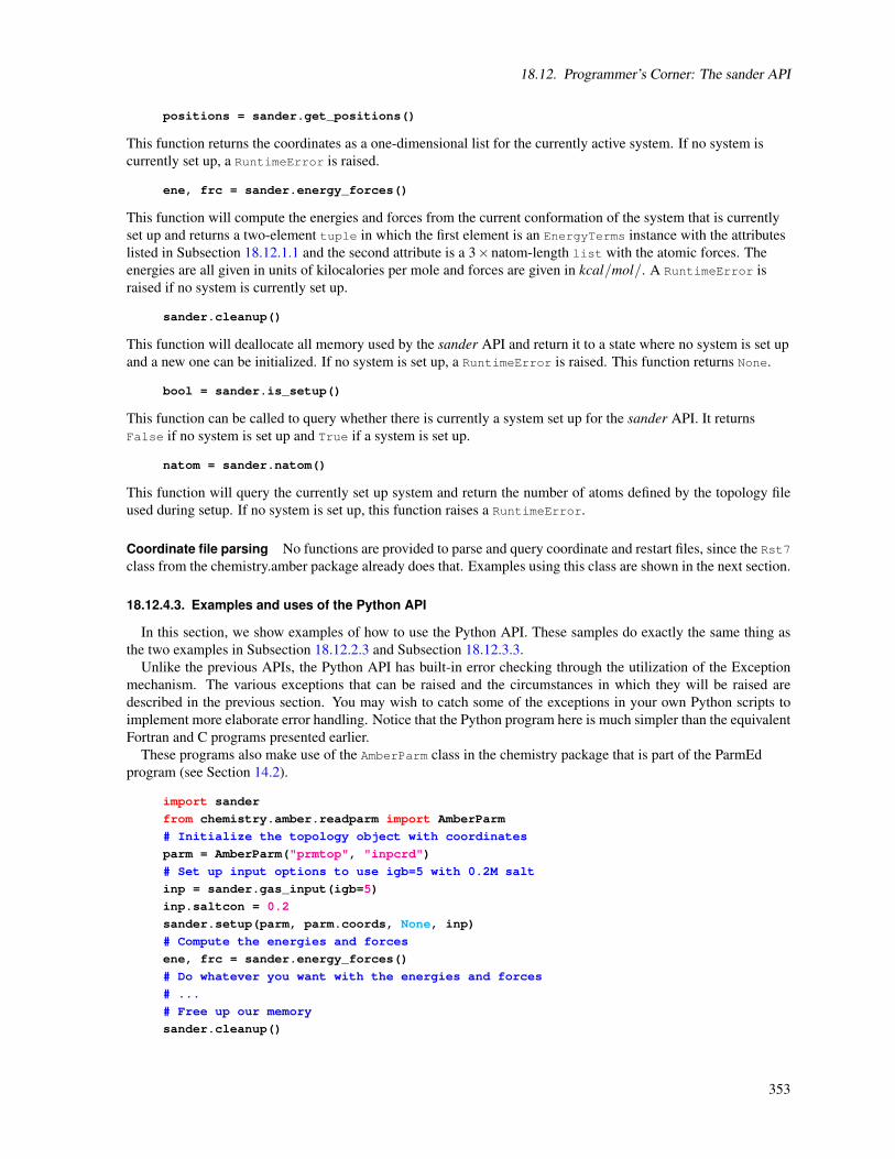
18.12. Programmer’s Corner: The sander API
positions = sander.get_positions()
This function returns the coordinates as a one-dimensional list for the currently active system. If no system iscurrently set up, a RuntimeError is raised.
ene, frc = sander.energy_forces()
This function will compute the energies and forces from the current conformation of the system that is currentlyset up and returns a two-element tuple in which the first element is an EnergyTerms instance with the attributeslisted in Subsection 18.12.1.1 and the second attribute is a 3×natom-length list with the atomic forces. Theenergies are all given in units of kilocalories per mole and forces are given in kcal/mol/. A RuntimeError israised if no system is currently set up.
sander.cleanup()
This function will deallocate all memory used by the sander API and return it to a state where no system is set upand a new one can be initialized. If no system is set up, a RuntimeError is raised. This function returns None.
bool = sander.is_setup()
This function can be called to query whether there is currently a system set up for the sander API. It returnsFalse if no system is set up and True if a system is set up.
natom = sander.natom()
This function will query the currently set up system and return the number of atoms defined by the topology fileused during setup. If no system is set up, this function raises a RuntimeError.
Coordinate file parsing No functions are provided to parse and query coordinate and restart files, since the Rst7class from the chemistry.amber package already does that. Examples using this class are shown in the next section.
18.12.4.3. Examples and uses of the Python API
In this section, we show examples of how to use the Python API. These samples do exactly the same thing asthe two examples in Subsection 18.12.2.3 and Subsection 18.12.3.3.
Unlike the previous APIs, the Python API has built-in error checking through the utilization of the Exceptionmechanism. The various exceptions that can be raised and the circumstances in which they will be raised aredescribed in the previous section. You may wish to catch some of the exceptions in your own Python scripts toimplement more elaborate error handling. Notice that the Python program here is much simpler than the equivalentFortran and C programs presented earlier.
These programs also make use of the AmberParm class in the chemistry package that is part of the ParmEdprogram (see Section 14.2).
import sander
from chemistry.amber.readparm import AmberParm
# Initialize the topology object with coordinates
parm = AmberParm("prmtop", "inpcrd")
# Set up input options to use igb=5 with 0.2M salt
inp = sander.gas_input(igb=5)
inp.saltcon = 0.2
sander.setup(parm, parm.coords, None, inp)
# Compute the energies and forces
ene, frc = sander.energy_forces()
# Do whatever you want with the energies and forces
# ...
# Free up our memory
sander.cleanup()
353

18. sander
The second example we provide shows how to use the Python API to compute the energy for a periodic systemusing a multiscale QM/MM Hamiltonian. We will treat residues 10, 11, 12, and 20 using the PDDG-PM3Hamiltonian. Also, rather than loading the inpcrd file directly into the AmberParm object, we use the openconstructor of the Rst7 class to read in the coordinate file. While this is exactly what the AmberParm class doesunder the hood, this approach is presented here to show how to use the Rst7 class in your own programs.
import sander
from chemistry.amber.readparm import AmberParm, Rst7
# Initialize the topology object with coordinates
parm = AmberParm("prmtop")
rst = Rst7.open("inpcrd")
# Set up input options to use PME with a 10A cutoff
inp = sander.gas_input(igb=5)
inp.cut = 10.0
qm_inp = sander.QmInputOptions()
qm_inp.qmmask = “:10-12,20”
qm_inp.qm_theory = “PDDG-PM3”
sander.setup(parm, rst.coords, rst.box, inp, qm_inp)
# Compute the energies and forces
ene, frc = sander.energy_forces()
# Do whatever you want with the energies and forces
# ...
# Free up our memory
sander.cleanup()
One final thing we will mention is that the sander Python API supports the context manager protocol! Theprevious example can be rewritten as
import sander
from chemistry.amber.readparm import AmberParm, Rst7
# Initialize the topology object with coordinates
parm = AmberParm("prmtop")
rst = Rst7.open("inpcrd")
# Set up input options to use PME with a 10A cutoff
inp = sander.gas_input(igb=5)
inp.cut = 10.0
qm_inp = sander.QmInputOptions()
qm_inp.qmmask = “:10-12,20”
qm_inp.qm_theory = “PDDG-PM3”
with sander.setup(parm, rst.coords, rst.box, inp, qm_inp):
# Compute the energies and forces
ene, frc = sander.energy_forces()
# Do whatever you want with the energies and forces
# ...
# Free up our memory
When the context manager is exited (i.e., when program execution is no longer inside the with block), sander isautomatically cleaned up. This occurs regardless of whether or not an error was raised during the execution of thecode within the with block. Notice how sander.cleanup() is no longer necessary.
18.12.4.4. Using the LES Python API
To use the LES functionality in Python, you need to import the sanderles package instead of the sander
package. Note that while nothing stops you from importing both the sander and sanderles packages in the samePython script, both packages will not work correctly in the same script.
354

19. pmemd
19.1. Introduction
PMEMD (Particle Mesh Ewald Molecular Dynamics) was initially a reimplementation of a subset of sanderfunctionality, although it has since diverged somewhat into the primary molecular dynamics engine within theAMBER Software suite, written with the primary goal of improving the performance of the most frequently usedmethods of sander. PMEMD supports Particle Mesh Ewald simulations, Generalized Born simulations, IsotropicPeriodic Sum, ALPB (Analytical Linearized Poisson-Boltzmann) and as of AMBER v16 gas phase simulationsusing both the AMBER and CHARMM Force fields.
One of the major additions to PMEMD in recent years has been addition of support for acceleration of PME,GB and IPS calculations using NVIDIA GPUs.[365–367] A detailed overview is provided in section 19.6
For the supported functionality, the input required and output produced are intended to exactly replicate sanderwithin the limits of machine roundoff differences. PMEMD simply runs more rapidly, scales better in parallel usingMPI, can be used profitably on significantly higher numbers of processors, can make use of NVIDIA GPUs andIntel Xeon Phis for acceleration and uses less resident memory. Dynamic memory allocation is used so memoryconfiguration is not required. PMEMD is ideal for molecular dynamics simulations of both small and large solvatedsystems for long periods of time, especially if supercomputer or GPU resources are available. Benchmark data isavailable on the Amber website, ambermd.org. Given the improvements in performance in both serial and parallelas well as the incredible performance offered by GPU acceleration it is adviseable to always use PMEMD in placeof sander if the simulation requirements are within the functionality envelope provided by PMEMD.
PMEMD accepts sander input files (mdin, prmtop, inpcrd, refc), and is also backward compatible in regard toinput to the same extent as sander. All options documented in the sander section of this manual should be properlyparsed and an error message generated if a requested feature is not supported.
19.2. Functionality
New functionality has been added to pmemd in release 16 of Amber including:
• Support for gas phase simulations (through igb=6) [cpu & gpu]
• Support for external electric fields [cpu]
• Support for the Charmm VDW Force switch [cpu & gpu]
• Support for Gaussian accelerated molecular dynamics [cpu & gpu]
and the following functionality, as of AMBER 16, is also now supported by the GPU version of pmemd in additionto the CPU version:
• Semi-Isotropic pressure scaling
• Enhanced NMR restraints and R^6 averaging support
• Expanded umbrella sampling support
• Constant pH and REMD Constant pH
In addition the following will soon be added via AMBER’s update mechanism during compilation:
• Support for Adaptively biased MD
355
19. pmemd
• Support for the upcoming Knights Landing Intel Xeon Phi on day of release
• Improved CPU performance and scaling
• Thermodynamic Integration, FEP and MBAR support on GPUs
As mentioned above, PMEMD is not a complete implementation of sander. Instead, it is intended to be a fastimplementation of the functionality most likely to be used by someone doing long time scale explicitly or implicitlysolvated systems. It also includes some additional functionality of it’s own.
Specifically the following functionality in sander is missing entirely:
imin=5 In &cntrl. Trajectory analysis is not supported.
nmropt=2 In &cntrl. A variety of NMR-specific options such as NOESY restraints, chemical shift restraints,pseudocontact restraints, and direct dipolar coupling restraints are not supported.
idecomp!=0 In &cntrl. Energy decomposition options, used in conjunction with mm_pbsa, are not supported.
ipol!=0 In &cntrl. Polarizable force field simulations are not supported.
igb==10 In &cntrl. Poisson-Boltzmann simulations are not supported.
ntmin>2 In &cntrl. XMIN and LMOD minimization methods are not supported.
Solvent Caps Solvent cap simulations are not supported.
itgtmd!=0 In &cntrl. Targeted molecular dynamics is not supported.
ievb!=0 In &cntrl. Empirical Valence Bond methods are not supported.
ifqnt!=0 In &cntrl. QM/MM methods are not supported.
&debugf namelist Use of the &debugf namelist is only supported in a very limited way. Specifically only thedo_charmm_dump_gold option is supported.
ineb!=0 In &cntrl. Nudged elastic band (NEB) calculations are not supported. These calculations are done bysander.MPI.
LES The Locally Enhanced Sampling method is not supported.
REM==2 The partial REMD method (for LES) is not supported
iamoeba!=0 In &cntrl. The amoeba polarizable potentials of Ren and Ponder are not supported in pmemd, al-though support is provided through a special pmemd.amoeba implementation provided as part of Am-ber 16.
The following &ewald options are supported, but only with the indicated default values:
ew_type=0 Only Particle Mesh Ewald calculations are supported. ew_type = 1 (regular Ewald calculations) mustbe done in sander.
nbflag=1 The nbflag option is ignored for MD, and all nonbonded list updates are scheduled based on "skin"checks. This is more reliable and has little cost. The variable nsnb still can be set and has an influenceon minimizations but is ignored during MD. For PME calculations, list building may also be scheduledbased on heuristics to suit load balancing requirements in multiprocessor runs.
nbtell=0 The nbtell option is not particularly useful and is ignored.
eedmeth=1 Only a cubic spline switch function (eedmeth = 1) for the direct sum Coulomb interaction is supported.This is the default, and most widely used setting for eedmeth. On some machine architectures, energiesand forces are actually splined as a function of r**2 to a higher precision than the cubic spline switch.
356

19.3. PMEMD-specific namelist variables
column_fft=0 This is a sander-specific performance optimization option. PMEMD uses different mechanisms toenhance performance, and ignores this option.
It is suggested that new PMEMD users simply take an existing sander mdin file and attempt a short 10-30 step run.The output will indicate whether or not PMEMD will handle the particular problem at hand for all the functionalitythat is supported by "standard" sander. For functionality that requires special builds of sander or sander-derivedexecutables (LES), there may be failures in namelist parsing.
19.3. PMEMD-specific namelist variables
The following namelist options are specific to PMEMD and generally relate to PMEMD specific performanceoptimizations: default values:
mdout_flush_interval In &cntrl, this variable can be used to control the minimum time in integer seconds between"flushes" of the mdout file. PMEMD DOES NOT use file flush() calls at all because flush functionalitydoes not work for all fortran compilers used in building pmemd. Thus, pmemd does an open/closecycle on mdout at a default minimum interval of 300 seconds. This interval can be changed withthis variable if desired in the range of 0-3600. If mdout_flush_interval is set to 0, then mdout willbe reopened and closed for each printed step. This functionality is provided in pmemd because somelarge systems have such large file i/o buffers that mdout will have 0 length on the disk through 100’s ofpsec of simulated time. The default of 300 seconds provides a good compromise between efficiencyand being able to observe the progress of the simulation.
mdinfo_flush_interval In &cntrl, this variable can be used to control the minimum time in integer seconds between"flushes" of the mdinfo file. PMEMD DOES NOT use file flush() calls at all because flush functionalitydoes not work for all fortran compilers used in building pmemd. Thus, pmemd does an open/closecycle on mdinfo at a default minimum interval of 60 seconds. This interval can be changed with thisvariable if desired in the range of 0-3600. Note that mdinfo under pmemd simply serves as a heartbeatfor the simulation at mdinfo_flush_interval, and mdinfo probably will not be updated with the last stepdata at the end of a run. If mdinfo_flush_interval is set to 0, then mdinfo will be reopened and closedfor each printed step.
es_cutoff, vdw_cutoff In &cntrl, these variables can be used to control the cutoffs used for vdw and electrostaticdirect force interactions in PME calculations separately. If you specify these variables, you shouldnot specify the cut variable, and there is a requirement that vdw_cutoff >= es_cutoff. These wereintroduced anticipating the need to support force fields where the direct force calculations are moreexpensive. For the current force fields, one can get slightly improved performance and about the sameaccuracy as one would get using a single cutoff. A good example would be using vdw_cutoff =9.0,es_cutoff =8.0. For this scenario, one gets about the accuracy in calculations associated with 9.0angstrom cutoffs, but at a cost intermediate between an 8.0 and a 9.0 angstrom cutoff.
no_intermolecular_bonds In &cntrl. New variable controlling molecule definition. If 1, any molecules (ie.,molecules as defined by the prmtop) joined by a covalent bond are fused to form a single molecule forpurposes of pressure and virial-related operations; if 0 then the old behaviour (use prmtop moleculedefinitions) pertains. The default is 1; a value of 0 is not supported with forcefields using extra points.This option was necessitated in order to efficiently parallelize model systems with extra points. Thisredefinition of molecules actually allows for a more correct treatment of molecules during pressure ad-justments and should produce better results with less strain on covalent bonds joining prmtop-definedmolecules, but if the default value is used for a NTP simulation, results will differ slightly relative tosander if any intermolecular bonding was applied in forming the prmtop (eg., a cyx-cyx bridge wasadded between two peptides that originated in a PDB file, with each peptide having its own "TER"card). If consistency with sander is more important to you, and you are not using extra points, thenyou may want to set no_intermolecular_bonds to 0.
357
19. pmemd
ene_avg_sampling In &cntrl. New variable controlling the number of steps between energy samples used inenergy averages. If not specified, then ntpr is used (default). To match the behaviour of sanderor PMEMD v9 or earlier, this variable should be set to 1. This variable is only used for MD, notminimization and will also effectively be turned off if ntave is in use (non-0) or RESPA is in use(nrespa > 1). It is a fairly common situation that it is completely unnecessary to sample the energiesevery step to get a good average during production, and this is costly in terms of performance. Thus,performance can be improved (with greatest improvements for the ensembles in the order NVE > NVT> NTP) without really losing anything of value by using the new default for energy average sampling(specify nothing).
use_axis_opt In &ewald. For parallel runs, the most favorable orientation of an orthogonal unit cell is with thelongest side in the Z direction. Starting with pmemd 3.00, internal coordinates were actually reori-ented to take advantage of this, and in high processor count runs on oblong unit cells, using axisoptimization can improve performance on the order of 10%. However, if a system has hotspots, theresults produced with axes oriented differently may vary by on the order of 0.05% relatively quickly.This effect has to do with the fact that axis optimization changes the order of LOTS of operations andalso the fft slab layout, and under mpi if the system has serious hotspots, shake will come up withslightly different coordinate sets. This is really only a problem in pathological situations, and thenit is probably mostly telling you that the situation is pathological, and neither set of results is morecorrect (typically the ewald error term is also high). In routine regression testing with over a dozentests, axis reorientation has no effect on results. Nonetheless, the defaults are now selected to be infavor of higher reproducibility of results. Axis optimization is only done for mpi runs in which anorthogonal unit cell has an aspect ratio of at least 3 to 2. It is turned off for all minimization runs andfor runs in which velocities are randomized (ntt = 2 or 3). If you want to force axis optimization, youmay set use_axis_opt = 1 in the &ewald namelist. If you set it to 0, you will force it off in scenarioswhere it would otherwise be used.
fft_grids_per_ang In &ewald. This variable may be used to set the desired reciprocal space fft grid density interms of fft grids/angstrom. The nearest grid dimensions, given the prime factors supported by theunderlying fft implementation, that meet or exceed this density will be used (ie., nfft1,2,3 are set basedon this specification). The default value is 1.0 grids/angstrom and gives very reasonable accuracy.PMEMD is actually more stringent now than sander in that it will meet or exceed the desired densityinstead of just approximating it. Thus, to get identical results with sander, one may have to specifygrid dimensions to be used with the nfft1,2,3 variables.
19.4. Slightly changed functionality
An I/O optimization has been introduced into PMEMD. If the user does not specify a value of NTWR then itdefaults to NSTLIM. In general, frequent writes of restrt, especially in runs with a high processor count or onGPUs, is wasteful. Also, if the mden file is being written, it is always written as formatted output, regardless of thevalue of ioutfm. SANDER now conforms to this convention regarding ioutfm and mden.
In thermodynamic integration calculations, the input format is different from SANDER. The differences areexplained in section 22.1 of the manual.
In addition, there are two command-line options unique to pmemd:
-l <logfile name> A name may be assigned to the log file on the command line.
-gpes <process_map_file> This option controls the distribution of threads in a multipmemd simulation and al-lows you to allocate threads to various processes however you want (rather than dividing up all threadsequally between each line of the groupfile). By default, the threads are allocated sequentially (that is, forN groups given M threads per group, or N*M threads total, threads 0 to M-1 will be assigned to the firstgroup, threads M to 2M-1 will be assigned to the second group, etc.). Using the -ng-nonsequential flag,threads will be allocated with a one-at-a-time approach. For instance, given the same setup as above, thefirst group gets threads 0, M, 2M, 3M, ... etc, the second group gets threads 1, M+1, 2M+1, 3M+1, ... etc.
358

19.5. Parallel performance tuning and hints
The process_map_file is a file that contains as many lines as you have groups (although the last line can beomitted, and the remaining unspecified threads will be assigned to the final group). Each line must containspace-delimited integers that correspond to the thread numbers you want assigned to that group. Each groupis assigned the threads listed in that line of the process_map_file. Every thread must be specified in theprocess_map_file, and no thread can be specified more than once.
19.5. Parallel performance tuning and hints
In order to achieve higher scaling, pmemd has implemented several performance algorithms, the most notableof which is the option of using a "block" or pencil fft rather than the usual slab fft algorithm. The block fftalgorithm allows the reciprocal space and fft workload to be distributed to more processors, but at a cost of highercommunications overhead, both in terms of the distributed fft transpose cost and in terms of communication ofthe data necessary to set up the fft grids in the first place. A number of variables in the &ewald namelist canbe used to control whether the slab or block fft algorithm is used, how the block division occurs, whether directforce work is also assigned to tasks doing reciprocal space and fft work, whether the master is given any force andenergy computation work to do, as opposed to being reserved strictly for handling output and loadbalancing, andthe frequency of atom ownership reassignment, an operation that counteracts rising communications costs causedby diffusion. The various namelist variables involved have all been assigned defaults that adapt to run conditions,and in general it is probably best that the user just use the defaults and not attempt to make adjustments. However,in some instances, fine tuning may yield slightly better performance. The variables involved include block_fft,fft_blk_y_divisor, excl_recip, excl_master, and atm_redist_freq. These are described further in the README underpmemd/src as well as in the sourcecode itself.
Performance depends not only on proper setup of hardware and software, but also on making good choices insimulation configuration. There are many tradeoffs between accuracy and cost, as one might expect, and under-standing all of these comes with experience. However, I would like to suggest a couple of good choices for yoursimulations, if you have facilities where you can routinely run at high processor count, say 32 processors or more.First of all, there is an implementation of binary trajectory files in pmemd and sander, based on the netCDF binaryfile format. This is invoked now using ioutfm == 1, assuming you have built either pmemd or sander with "bintraj"support. Using this output format, i/o from the master process will be more efficient and your filesize will be abouthalf what it would otherwise be. In Amber, ptraj can read these new netCDF trajectory files and can convert themto ASCII format if needed. At really high processor count using the netCDF format can be on the order of 10%more efficient than using the standard formatted trajectory output. Secondly, other simulation packages typicallyuse multiple timestepping (respa) methods as an efficiency measure. These methods typically sample reciprocalspace forces for PME less frequently. Due to the limited use of such methods by Amber users this approach hasnot been optimized in pmemd and hence while this can slightly improve performance for pmemd at low processorcount, at higher processor counts using respa typically makes loadbalancing less efficient leading to a net loss ofperformance. If you wish to use respa for pme simulations (done typically by setting nrespa to 2 or 4), then youshould check whether you actually get better performance. You may well not, and it will be at a cost of a loss inaccuracy. Using respa for generalized Born simulations is fine in all cases, however.
19.6. GPU Accelerated PMEMD
One of the newer features of PMEMD, is the ability to use NVIDIA GPUs to accelerate both explicit solventPME and implicit solvent GB simulations [365–367]. This work is by Ross Walker at the San Diego Supercom-puter Center and Scott Le Grand in collaboration with NVIDIA. While this GPU acceleration is considered to beproduction ready, and has been heavily used since its release as part of AMBER 11, it is still evolving and has notbeen tested to the same extent as the CPU code; users should exercise caution when using this code. The errorchecking is not as verbose in the GPU code as it is on the CPU. In particular, simulation failures, such as atomcollisions or other simulation instabilities, will manifest themselves as CUDA launch errors or GPU download fail-ures and not as informative error messages. If you encounter problems during a simulation on the GPU you shouldfirst try to run the identical simulation on the CPU to ensure that it is not your simulation setup which is causing
359

19. pmemd
problems. Feedback and questions should be posted to the Amber mailing list (see http://lists.ambermd.org/ ).This section of the manual describes the feature set, installation, performance and accuracy considerations and
other aspects of GPUs at the time of Amber’s release. However, the rapidly changing nature of this field meansthat frequent updates are likely. You should refer to the web page http://ambermd.org/gpus/ for the most up to dateinformation.
19.6.1. Supported Features
The GPU accelerated version of PMEMD supports both explicit solvent PME simulations in all three canonicalensembles (NVE, NVT and NPT) and implicit solvent Generalized Born simulations. It has been designed tosupport as many of the standard PMEMD features as possible, however, there are some current limitations that aredetailed below. Some of these may be addressed in the future, and patches released, with the most up to date listposted on the web page. The following options are NOT supported:
1. ibelly 6= 0 Simulations using belly style constraints are not supported.
2. icfe 6= 0 Support for TI is not currently implemented (but an update to support this in AMBER 16 is planned).
3. igb 6= 0 && cut < systemsize GPU accelerated implicit solvent GB simulations do not support a cutoff.
4. nmropt > 1 Support is not currently available for nmropt > 1. In addition for nmropt = 1 only features that donot change the underlying force field parameters are supported. For example umbrella sampling restraintsare supported as is Jarzynski sampling as well as simulated annealing functions such as variation of Temp0with simulation step. However, varying the VDW parameters with step is not supported.
5. nrespa 6= 1 No multiple time stepping is supported.
6. vlimit 6= -1 For performance reasons the vlimit function is not implemented on GPUs.
7. imin = 1 with MPI Minimization is currently only supported for single GPU runs.
8. es_cutoff 6= vdw_cutoff Independent cutoffs for electrostatics and van der Waals are not supported on GPUs.
9. order > 4 PME interpolation orders of greater than 4 are not supported at present.
10. emil_do_calc 6= 0 Emil is not supported on GPUs.
11. lj1264 6= 0 The 12-6-4 potential is not supported on GPUs.
12. iemap > 0 EMAP restraints are not supported on GPUs.
13. isgld > 0 Self guided langevin dynamics are not supported on GPUs.
Additionally there are some minor differences in the output format. For example the Ewald error estimate is notcalculated when running on a GPU. It is recommended that you first run a short simulation using the CPU code tocheck that the Ewald error estimate is reasonable and that your system is stable. The above limitations are testedfor in the code; however, it is possible that there are additional simulation features that have not been implementedor tested on GPUs.
19.6.2. New in Amber 16
Amber 16 represents a continued evolution of the Amber GPU MD ecosystem with a number of additions tofunctionality, support for new hardware and extensive optimization appearing in the latest release. One of thekey advances in Amber 16 is code optimization that provides a speed boost of approximately 30% on the currentMaxwell generation (M40, M60, GTX980, GTX980TI and GTX-Titan-X) hardware. At the time of writing asingle node containing 4 GTX-Titan-X GPUs achieves over 550ns/day for the DHFR 4fs NVE benchmark withan aggregate throughput of over 1.4 microseconds per day possible. This makes AMBER 16 the world’s fastestmolecular dynamics software package on commodity hardware.
Additional improvements in Amber 16 include:
360

19.6. GPU Accelerated PMEMD
• Support for semi-isotropic pressure scaling
• Support for the Charmm VDW force switch
• Enhances NMR restraint support and R^6 averaging support
• Gaussian accelerated molecular dynamics
• Expanded umbrella sampling support
• Constant pH and REMD Constant pH support
• Support and significant performance improvements for the latest Maxwell and the soon to be released PascalGPUs from NVIDIA
• Adaptively biased MD (coming soon via automatic update)
• Thermodynamic Integration, FEP and MBAR (coming soon via an automatic update)
19.6.3. Supported GPUs
GPU accelerated PMEMD has been implemented using CUDA and thus will only run on NVIDIA GPUsat present. Due to accuracy concerns with pure single precision the code uses a custom designed hybridsingle/double/fixed-precision model termed SPFP. This places the requirement that the GPU hardware supportsboth double precision and integer atomics meaning only GPUs with hardware revision 2.0 (C2050 / GTX480) andlater can be used. Support for hardware revision 1.3 (C1060 / GTX295) was present in previous versions of thecode but for code complexity and maintenance reasons has been deprecated as of AMBER 14. Support is providedfor Tesla, Quadro and GeForce GPUs and almost all mid to high end cards are supported. You are encouraged tovisit the AMBER website (ambermd.org/gpus/) for an update to date list of supported hardware and performancenumbers.
You should ensure that all GPUs on which you plan to run PMEMD are connected to PCI-E 2.0 x16 lane slotsor better. For peer to peer communication (required for multi-GPU scaling) the cards to be used need to be in thesame PCI-E domain. If this is not the case then you will likely see significantly degraded performance in parallel.For more information, and details of optimium hardware designs. please see Recommended Hardware under theGPU section of the AMBER website (http://ambermd.org/gpus/ ).
Support is provided for single GPU and multiple GPU runs. Employing multiple GPUs in a single simulationrequires MPI and the pmemd.cuda.MPI executable. If you have multiple simulations to run then the recommendedmethod is to use one GPU per job. The pmemd GPU code has been developed in such a way that for single GPUruns the PCI-E bus is only used for I/O. This sets AMBER apart from other MD packages since it means the CPUspecs do not feature in the GPU code performance. As such low end economic CPUs can be used. Addition-ally it means that in a system containing 4 GPUs 4 individual calculations can be run at the same time withoutinterfering with each other’s performance. Selection of which GPU is used for single GPU runs is automatic ifthe GPUs are set to process exclusive mode (nvidia-smi -c 3) but the recommended approach is to use theCUDA_VISIBLE_DEVICES environment variable to select which GPU should be used. For parallel runs youspecify the same number of MPI threads as you have GPUs you want to use. The code will automatically use peerto peer communication if available. Multi-GPU runs require the GPUs to be set to default mode (nvidia-smi -c
0). More details are provided in section 19.6.6.
19.6.4. Accuracy Considerations
The nature of current generation GPUs is such that single precision arithmetic is considerably faster (>200xfor M40, >23x for K10 and >2x for K20) than double precision arithmetic. This poses an issue when trying toobtain good performance from GPUs. Traditionally the CPU code in Amber has always used double precisionthroughout the calculation. While this full double precision approach has been implemented in the GPU code itgives very poor performance and so the default precision model used when running on GPUs is a combination of
361

19. pmemd
single and fixed precision, termed hybrid precision (SPFP), that is discussed in further detail in references [365–367]. This approach uses single precision for individual calculations within the simulation but fixed scaled integerprecision for all accumulations. It also uses fixed precision for shake calculations and for other parts of the codewhere loss of precision was deemed to be unacceptable. Tests have shown that energy conservation is equivalentto the full double precision code and specific ensemble properties, such as order parameters, match the full doubleprecision CPU code. Previous acceleration approaches, such as the MDGRAPE-accelerated sander, have usedsimilar hybrid precision models and thus we believe that this is a reasonable compromise between accuracy andperformance. The user should understand though that this approach leads to rapid divergence between GPU andCPU simulations, similar to that observed when running the CPU code across different processor counts in parallelbut occuring much more rapidly. Ultimately though this is simply a cosmetic consideration since any statisticalmechanical properties should converge to the same values.
While the default precision model is currently the hybrid SPFP model two additional precision models havebeen implemented within version 16 of the GPU code to facilitate advanced testing and comparison. The choice ofdefault precision model may change in the future based on the outcome of detailed validation tests of the differentapproaches. The precision models supported, all of which are built automatically at compile time are:
• SPFP - (Default) Use a combination of single precision for calculation and fixed precision for accumulation.This approach is believed to provide the optimum tradeoff between accuracy and peformance and hence atthe time of release is the default model invoked when using the executable pmemd.cuda.
• DPFP - Use double precision (and double precision equivalent fixed precision) for the entire calculation.This provides for careful regression testing against the CPU code. It makes no additional approximationsabove and beyond the CPU implementation and would be the model of choice if performance was not aconsideration. On v2.0 NVIDIA hardware (e.g. M2090) the performance is approximately half that of theSPFP model while on v3.0 NVIDIA hardware (e.g. K10) the performance is substantially less than the SPFPmodel.
• SPXP - (Experimental) Use single precision for calculation and a combination of 32 bit integer accumulationstrategies to approximate 48 bit precision in the summation stage. This precision model has been designedto provide future proofing of performance on next and later generation hardware designs. It is consideredexperimental at present and should not be used for production simulations except as a way to test how themodel performs.
19.6.5. Installation and Testing
The GPU version of PMEMD is called pmemd.cuda (or pmemd.cuda.MPI for the multi GPU version) and mustbe built separately from the standard serial and parallel installations. Before attempting to build the GPU versionof PMEMD you should have built and tested at least the serial version of Amber and preferably the parallel versionas well. This will help to ensure that basic issues relating to standard compilation on your hardware and operatingsystem do not lead to confusion with GPU related compilation and testing problems. You should also be familiarwith Amber’s compilation and test procedures.
It is assumed that you have already correctly installed and tested CUDA support on your GPU. Addition-ally the environment variable CUDA_HOME should be set to point to your NVIDIA Toolkit installation and$CUDA_HOME/bin/ should be in your path. At the time of release CUDA 7.5 or later is required with 7.5 havingbeen tested and officially supported.
Building and Testing the GPU code
In a change from previous versions of Amber the GPU compilation and testing procedure has been simplifiedsuch that all three precision models are automatically built and the testing procedure has been made more reliablewith less false negatives during testing.
Assuming you have a working CUDA installation you can build all three precision models (pmemd.cuda_SPFP,pmemd.cuda_DPFP and pmemd.cuda_SPXP) with pmemd.cuda linked to pmemd.cuda_SPFP as follows:
362
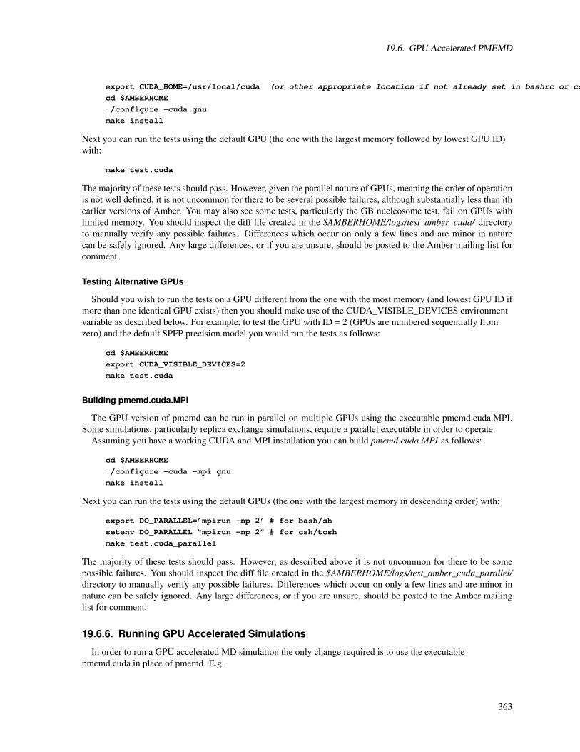
19.6. GPU Accelerated PMEMD
export CUDA_HOME=/usr/local/cuda (or other appropriate location if not already set in bashrc or cshrc)
cd $AMBERHOME
./configure -cuda gnu
make install
Next you can run the tests using the default GPU (the one with the largest memory followed by lowest GPU ID)with:
make test.cuda
The majority of these tests should pass. However, given the parallel nature of GPUs, meaning the order of operationis not well defined, it is not uncommon for there to be several possible failures, although substantially less than ithearlier versions of Amber. You may also see some tests, particularly the GB nucleosome test, fail on GPUs withlimited memory. You should inspect the diff file created in the $AMBERHOME/logs/test_amber_cuda/ directoryto manually verify any possible failures. Differences which occur on only a few lines and are minor in naturecan be safely ignored. Any large differences, or if you are unsure, should be posted to the Amber mailing list forcomment.
Testing Alternative GPUs
Should you wish to run the tests on a GPU different from the one with the most memory (and lowest GPU ID ifmore than one identical GPU exists) then you should make use of the CUDA_VISIBLE_DEVICES environmentvariable as described below. For example, to test the GPU with ID = 2 (GPUs are numbered sequentially fromzero) and the default SPFP precision model you would run the tests as follows:
cd $AMBERHOME
export CUDA_VISIBLE_DEVICES=2
make test.cuda
Building pmemd.cuda.MPI
The GPU version of pmemd can be run in parallel on multiple GPUs using the executable pmemd.cuda.MPI.Some simulations, particularly replica exchange simulations, require a parallel executable in order to operate.
Assuming you have a working CUDA and MPI installation you can build pmemd.cuda.MPI as follows:
cd $AMBERHOME
./configure -cuda -mpi gnu
make install
Next you can run the tests using the default GPUs (the one with the largest memory in descending order) with:
export DO_PARALLEL=’mpirun -np 2’ # for bash/sh
setenv DO_PARALLEL “mpirun -np 2” # for csh/tcsh
make test.cuda_parallel
The majority of these tests should pass. However, as described above it is not uncommon for there to be somepossible failures. You should inspect the diff file created in the $AMBERHOME/logs/test_amber_cuda_parallel/directory to manually verify any possible failures. Differences which occur on only a few lines and are minor innature can be safely ignored. Any large differences, or if you are unsure, should be posted to the Amber mailinglist for comment.
19.6.6. Running GPU Accelerated Simulations
In order to run a GPU accelerated MD simulation the only change required is to use the executablepmemd.cuda in place of pmemd. E.g.
363

19. pmemd
$AMBERHOME/bin/pmemd.cuda -O -i mdin -o mdout -p prmtop \
-c inpcrd -r restrt -x mdcrd
This will automatically run the calculation on the GPU with the most memory even if that GPU is already in use.If you have only a single CUDA capable GPU in your machine then this is fine; however if you want to controlwhich GPU is used, or you want to run multiple independent simulations using different GPUs, then you manuallyneed to specify the GPU to use with the CUDA_VISIBLE_DEVICES environment variable.
CUDA_VISIBLE_DEVICES Specifies which GPU should be used for running a GPU accelerated PMEMD cal-culation. This is based on the hardware ID of the GPU card which can be obtained by unsettingthe variable (unset CUDA_VISIBLE_DEVICES) and running the deviceQuery command from theNVIDIA CUDA SDK. Valid values are a list of integers from 0 to 32. Multiple GPUs may be listedwith commas in between them, and the one with the most memory will be selected. For example:
export CUDA_VISIBLE_DEVICES=1,3
$AMBERHOME/bin/pmemd.cuda -O -i mdin -o mdout -p prmtop \
-c inpcrd -r restrt -x mdcrd
In this way it is possible to make use of multiple GPUs in a single node for multiple simultaneous calculations.When running a single calculation across multiple GPUs using pmemd.cuda.MPI it also allows the selection ofspecific GPUs on specific nodes. For example running a 2 GPU job with mpirun -np 2 pmemd.cuda.MPI withthe above listed CUDA_VISIBLE_DEVICES would automatically use the second (id=1) and fourth (id=3) GPUin the node. The multi GPU code will avoid assigning MPI GPU tasks to the same GPU if sufficient GPUs arevisible. For a more indepth explanation of running GPU accelerated calculations, including how to utilize the peerto peer support in parallel please refer to the GPU section of the AMBER website (http://ambermd.org/gpus/).
19.6.7. Considerations for Maximizing GPU Performance
There are a number of considerations above and beyond those typically used on a CPU for maximizing theperformance achievable for a GPU accelerated PMEMD simulation. The following provides some tips for ensuringgood performance.
1. Avoid using small values of NTPR, NTWX, NTWV, NTWE and NTWR. Writing to the output, restartand trajectory files too often can hurt performance even on CPU runs; however, this is more acute for GPUaccelerated simulations because there is a substantial cost in copying data to and from the GPU. Performanceis maximized when CPU to GPU memory synchronizations are minimized. This is achieved by computingas much as possible on the GPU and only copying back to CPU memory when absolutely necessary. Thereis an additional overhead in that performance is boosted by only calculating the energies when absolutelynecessary, hence setting NTPR or NTWE to low values will result in excessive energy calculations. Youshould typically not set any of these values to less than 100 (except 0 to disable them) and ideally use valuesof 1000 or more. >100000 for NTWR is ideal, or even better let it just default fo NSTLIM.
2. Avoid setting ntave 6= 0. Turning on the printing of running averages results in the code needing to calculateboth energy and forces on every step. This can lead to a performance loss of 8% or more when running onthe GPU. This can also affect performance on CPU runs although the difference is not as marked. Similararguments apply to setting the value of ene_avg_sampling to small values.
3. Avoid using the NPT ensemble (ntb=2) when it is not required; if needed make use of the Monte Carlobarostat (barostat=2). Performance will generally be NVE>NVT>NPT (NVT~NPT for barostat=2).
4. Avoid the use of GBSA in implicit solvent GB simulations unless required. The GBSA term is calculated onthe CPU and thus requires a synchronization between GPU and CPU memory on every MD step as opposedto every NTPR or NTWX steps when running without this option.
5. Use the Berendsen Thermostat (ntt=1) or Anderson Thermostat (ntt=2) instead of the Langevin Thermostat(ntt=3). Langevin simulations require very large numbers of random numbers which slows performanceslightly.
364

19.7. Intel® Many Integrated Core Architecture
6. Do not assume that for small systems the GPU will always be faster. Typically for GB simulations of lessthan 150 atoms and PME simulations of less than 5,000 atoms it is not uncommon for the CPU version ofthe code to outperform the GPU version on a single node. Typically the performance differential betweenGPU and CPU runs will increase as atom count increases. Additionally the larger the non-bond cutoff usedthe better the GPU to CPU performance gain will be.
7. When running in parallel across multiple GPUs you should restrict jobs to a single node and select GPUsthat are on the same PCIe domain and thus can communicate via peer to peer. For a discussion of PCIetopologies in modern hardware see the following writeup http://tinyurl.com/h469f73. For most budget 4GPU nodes gpus 0 and 1 can typically communicate via peer to peer and gpus 2 and 3 can communicate viapeer to peer. Thus you should not attempt to run a simulation across GPU combinations 0 and 2, or 0 and 3or 1 and 2 or 1 and 3. The mdout file contains a section that indicates if peer to peer support is enabled.
8. Turn off ECC (Tesla models C2050 and later). ECC can cost you up to 10% in performance. You shouldverify that your GPUs are working correctly, and not giving ECC errors for example before attempting this.You can turn this off on Fermi based cards and later by running the following command for each GPU ID asroot, followed by a reboot:
nvidia-smi -g 0 --ecc-config=0 (repeat with -g x for each GPU ID)
Extensive testing of AMBER on a wide range of hardware has established that ECC has little to no benefiton the reliability of AMBER simulations. This is part of the reason it is acceptable (see recommendedhardware) to use the GeForce gaming cards for AMBER simulations. For more details of ECC and MDsimulations see the following paper [368].
9. If you see that performance when running multiple - multi-GPU runs is bad. That is that say you run 2 x2GPU jobs and they don’t both run at full speed as if the other job was never running then make sure you turnoff thread affinity within your MPI implementation or at least set each MPI thread to use a difference core.In our experience MPICH does not have this on by default and so no special settings are needed howeverboth MVAPICH and OpenMPI set thread affinity by default. This would actually be useful if they did it inan intelligent way. However, it seems they pay no attention to load or even other MVAPICH or OpenMPIruns and always just assign from core 0. So 2 x 2 GPU jobs are, rather foolishly, assigned to cores 0 and 1in both cases. The simplest solution here is to just disable thread affinity as follows:
a) MVAPICH: export MV2_ENABLE_AFFINITY=0; mpirun -np 2 ...
b) OpenMPI: mpirun –bind-to none -np 2 ...
10. Turn on boost clocks if supported. Newer GPUs from NVIDIA, such as the K40 and K80, support boostclocks which allow the clock speed to be increased if there is power and temperature headroom. This mustbe turned on to obtain optimum performance with AMBER. If you have a K40 or newer GPU supportingboost clocks then run the following:
• K40: sudo nvidia-smi -i 0 -ac 3004,875 which puts device 0 into the highest boost state.
• K80: sudo nvidia-smi -i 0 -ac 2505,875
To return to normal do: sudo nvidia-smi -rac
To enable this setting without being root do: nvidia-smi -acp 0
19.7. Intel® Many Integrated Core Architecture
Note this section refers to the Intel Knights Corner Xeon Phi support that was included in Amber v16 at the timeof release. An extensive update is planned for release in late June 2016 to support the Intel Knights Landing XeonPhi which will be released at that time. You should refer to the Xeon Phi section of the Amber website for the mostup to date information (ambermd.org/xeon_phi/).
365

19. pmemd
One of the newest features of PMEMD is support for Intel MIC Products, such as Intel® Xeon PhiTM copro-cessors. Intel MIC Architecture support in PMEMD includes both native and offload mode in Amber 16. Theseversions of the PMEMD engine are considered experimental and there is no guarantee of any performance im-provement. However, this support should produce results directly comparable to the CPU implementation due tothe floating-point consistency of Intel’s processors. Any differences in tests will be a consequence of floating-pointrounding differences in hardware. Support for Intel® MIC Architecture in PMEMD is an ongoing project andtherefore frequent updates are likely. Improved performance can be expected in upcoming patches.
Support for the Intel MIC Architecture in Amber 1 offers two modes:• MIC native mode: allows all the functionality of the PMEMD engine to be run on Intel® Xeon PhiTM
coprocessors in native mode in either serial or parallel (MPI).
• MIC offload mode: offloads a portion of the direct sum calculation in a standard PME simulation to theIntel® Xeon PhiTM coprocessor for improved performance. We are anticipating in later releases to extendsupport to most functionality of PMEMD, which would include offloading to the Intel® Xeon PhiTM copro-cessor for Thermodynamic Integration (TI) and Isotropic Periodic Sum (IPS) simulations. Recommendedsystem size to be explored using the MIC offload version of PMEMD is >200,000 atoms in order to benefitfrom performance improvements. The MIC offload version of PMEMD requires Intel®’s MPI library whichis included in the Intel® Cluster Studio XE compiler package.
The supported Intel® Xeon PhiTM product family includes the Intel® Xeon PhiTM coprocessor 3100/5100/7100series. (Intel, Xeon, and Intel Xeon Phi are trademarks of Intel Corporation in the U.S. and/or other countries.)
Before attempting to build these versions you should have built and tested the serial and parallel CPU versionsof Amber (pmemd and pmemd.MPI) with the Intel compiler suite and Intel MPI. This will help to ensure thatbasic issues relating to standard compilation on your hardware and operating system do not lead to confusionwith coprocessor related compilation and testing problems. It is recommended that you are familiar with buildingand running simple code in native/offload mode on an Intel® Xeon PhiTM Coprocessor, which is described inhttps://software.intel.com/mic-developer. You should also be familiar with Amber’s compilation procedures.
19.7.1. MIC Native Model
The MIC native version supporting Intel® Xeon PhiTM coprocessors is called pmemd.mic_native (orpmemd.mic_native.MPI for running simulations in parallel on the coprocessor using MPI) and must be built sepa-rately from the standard serial and parallel installations.
Building PMEMD serial for Intel® Xeon PhiTM Coprocessors (native mode)
Assuming you have installed Intel® Parallel Studio XE version 2013 or later, you can build pmemd.mic_nativeas follows:
cd $AMBERHOME
./configure -mic_native intel
make install
Building PMEMD parallel for Intel® Xeon PhiTM Coprocessors (native mode)
PMEMD parallel for Intel® Xeon PhiTM coprocessors can only be built using the MPI (mpiicc/mpiifort) fromthe Intel® Cluster Studio XE product, which is supported in Amber through the use of a new MPI flag(-intelmpi). Build pmemd.mic_native.MPI as follows:
cd $AMBERHOME
./configure -mic_native -intelmpi intel
make install
366

19.7. Intel® Many Integrated Core Architecture
It is possible to run across multiple Intel® Xeon® processors and Intel® Xeon Phi™ coprocessors, even on acluster, with this implementation. However, it is a functional implementation and not performance optimized atthis time. Detailing how to run this way is beyond the scope of the current manual; however to see how to do thiswith MPI applications in general, see
http://software.intel.com/en-us/articles/using-the-intel-mpi-library-on-intel-xeon-phi-coprocessor-systems .
Running simulations on Intel® Xeon PhiTM Coprocessors (native mode)
In order to run a simulation on the Intel® Xeon Phi™ coprocessor, it is advised that you read the Intel®Xeon Phi™ Coprocessor Developer’s Quick Start Guide (http://software.intel.com/en-us/articles/intel-xeon-phi-coprocessor-developers-quick-start-guide) in addition to the instructions given here. This guide includes a de-scription of the Intel® Manycore Platform Software Stack (Intel® MPSS), which enables the wide range of usagemodels that Intel® Xeon Phi™ coprocessors support. Running a simulation on the coprocessor in native moderequires that all files and binaries be visible to the coprocessor. Either mount your file system on the coproces-sor (requires root access) or explicitly transfer the binaries, libraries and input files to the /tmp directory on thecoprocessor.
Note: Mounting requires the Amber directory plus any additional libraries used in an Amber simulation to bevisible to the coprocessor.
Running simulations with a mounted filesystem:
1. To mount a filesystem please follow instructions available in the Intel MPSS readme file. You can also followthe instructions in http://software.intel.com/sites/default/files/article/373934/system-administration-for-the-intel-xeon-phi-coprocessor.pdf
2. Mount your AMBERHOME directory, working directory, Intel compiler directory, Intel MPI_HOME direc-tory (for parallel run), and MKL_HOME directory (if MKL is used) on the coprocessor.
3. Add the following environment variables to a file (source_knc.sh in this example), which will be sourced onexecution of pmemd.mic_native:
export LD_LIBRARY_PATH=$LD_LIBRARY_PATH:$INTEL_COMPILER_HOME/lib/mic/
export LD_LIBRARY_PATH=$LD_LIBRARY_PATH:$MKL_HOME/lib/mic/
export LD_LIBRARY_PATH=$LD_LIBRARY_PATH:$MPI_HOME/mic/lib/
export PATH=$PATH:$MPI_HOME/mic/bin
4. Run a simulation from your working directory on the host (CPU) with a mounted filesystem:
ssh mic0 "source source_knc.sh; \
$AMBERHOME/bin/pmemd.mic_native -O -i mdin -o mdout -p prmtop -c inpcrd"
Running simulations without a mounted filesystem:
1. Upload the Intel® Xeon Phi™ coprocessor version of the Intel compiler library to the coprocessor:
scp -r $INTEL_COMPILER_HOME/lib/mic/* mic0:/tmp/
2. Similarly, upload the coprocessor versions of the MPI and MKL libraries:
scp -r $INTEL_MPI_HOME/mic/lib/* mic0:/tmp/
scp -r $INTEL_MPI_HOME/lib/mic/* mic0:/tmp/
3. Upload the coprocessor version of PMEMD (pmemd.mic_native or pmemd.mic_native.MPI) and your work-ing directory (containing the input fies for simulation):
scp -r $AMBERHOME/bin/pmemd.mic_native mic0:/tmp/
scp -r working_directory/* mic0:/tmp/
367

19. pmemd
4. Change the permissions of the libraries and binaries so that they are executable on the coprocessor:
chmod 777 -R /tmp/*
5. Finally run the simulation from the host:
ssh mic0 "export LD_LIBRARY_PATH=/tmp/; cd /tmp; \
./pmemd.mic_native -O -i mdin -o mdout -p prmtop -c inpcrd"
19.7.2. MIC Offload Mode
The MIC offload version supporting Intel® Xeon PhiTM coprocessors is called pmemd.mic_offload.MPI andmust be built separately from the standard parallel installation. MIC offload is not available in serial.
Building PMEMD for Intel® Xeon PhiTM Coprocessors (offload mode)
Assuming you have installed Intel® Parallel Studio XE version 2013 or later, you can buildpmemd.mic_offload.MPI as follows:
cd $AMBERHOME
./configure -mic_offload intel
make install
There is no need to specify the -intelmpi flag as this is the default behavior of the configure script.
Testing PMEMD for Intel® Xeon PhiTM Coprocessors (offload mode)
You can run the test suite using the MIC coprocessor with:
make test.mic_offload
The majority of these tests should pass. However, given the parallel nature of the MIC coprocessor, meaning theorder of operation is not well defined, it is not uncommon for there to be several "possible FAILURES". You shouldinspect the .dif file created in the $AMBERHOME/logs/test_amber_mic_offload/ directory to manually verify any"possible FAILURES". Differences that occur on only a few lines and are minor in nature can be safely ignored.Any large differences, or if you are unsure, should be posted to the Amber mailing list for comment.
Running simulations on Intel® Xeon PhiTM Coprocessors (offload mode)
Unlike MIC native mode, once PMEMD has been configured with the -mic_offload flag and compiled, noadditional steps are required to run pmemd.mic_offload.MPI. Work is automatically offloaded to the Intel MICArchitecture.
Execute the following command on the host to run a simulation in MIC offload mode:
mpirun -np 8 $AMBERHOME/bin/pmemd.mic_offload.MPI -O
Note: Choose the number of MPI processes to suit the specifications of the host CPU, e.g. 8 MPI processes foran Intel Xeon E5-2680 8 core processor, in order to achieve optimum performance. In the initial support for MICoffload in PMEMD, the amount of offloaded work to the coprocessor increases and settles to a stable value afterrunning multiple time steps governed by the Amber load balancer. Thus, it is recommended that the simulationshould run for at least 200 time steps to benefit from the coprocessor.
368
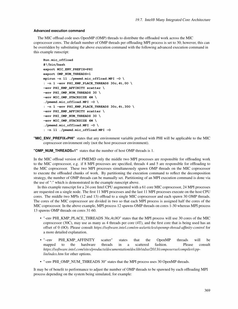
19.7. Intel® Many Integrated Core Architecture
Advanced execution command
The MIC offload code uses OpenMP (OMP) threads to distribute the offloaded work across the MICcoprocessor cores. The default number of OMP threads per offloading MPI process is set to 30; however, this canbe overridden by substituting the above execution command with the following advanced execution command inthis example runscript:
Run.mic_offload
#!/bin/bash
export MIC_ENV_PREFIX=PHI
export OMP_NUM_THREADS=1
mpirun -n 11 ./pmemd.mic_offload.MPI -O \
: -n 1 -env PHI_KMP_PLACE_THREADS 30c,4t,0O \
-env PHI_KMP_AFFINITY scatter \
-env PHI_OMP_NUM_THREADS 30 \
-env MIC_OMP_STACKSIZE 4M \
./pmemd.mic_offload.MPI -O \
: -n 1 -env PHI_KMP_PLACE_THREADS 30c,4t,30O \
-env PHI_KMP_AFFINITY scatter \
-env PHI_OMP_NUM_THREADS 30 \
-env MIC_OMP_STACKSIZE 4M \
./pmemd.mic_offload.MPI -O \
: -n 11 ./pmemd.mic_offload.MPI -O
"MIC_ENV_PREFIX=PHI" states that any environment variable prefixed with PHI will be applicable to the MICcoprocessor environment only (not the host processor environment).
"OMP_NUM_THREADS=1" states that the number of host OMP threads is 1.
In the MIC offload version of PMEMD only the middle two MPI processes are responsible for offloading workto the MIC coprocessor, e.g. if 8 MPI processes are specified, threads 4 and 5 are responsible for offloading tothe MIC coprocessor. These two MPI processes simultaneously spawn OMP threads on the MIC coprocessorto execute the offloaded chunks of work. By partitioning the execution command to reflect the decompositionstrategy, the number of OMP threads can be manually set. Partitioning of an MPI execution command is done viathe use of ":" which is demonstrated in the example runscript above.
In this example runscript for a 24 core Intel CPU augmented with a 61 core MIC coprocessor, 24 MPI processesare requested on a single node. The first 11 MPI processes and the last 11 MPI processes execute on the host CPUcores. The middle two MPIs (12 and 13) offload to a single MIC coprocessor and each spawn 30 OMP threads.The cores of the MIC coprocessor are divided in two so that each MPI process is assigned half the cores of theMIC coprocessor. In the above example, MPI process 12 spawns OMP threads on cores 1-30 whereas MPI process13 spawns OMP threads on cores 31-60.
• "-env PHI_KMP_PLACE_THREADS 30c,4t,0O" states that the MPI process will use 30 cores of the MICcoprocessor (30C), may use as many as 4 threads per core (4T), and the first core that is being used has anoffset of 0 (0O). Please consult https://software.intel.com/en-us/articles/openmp-thread-affinity-control fora more detailed explanation.
• "–env PHI_KMP_AFFINITY scatter" states that the OpenMP threads will bemapped to the hardware threads in a scattered fashion. Please consulthttps://software.intel.com/sites/products/documentation/doclib/stdxe/2013/composerxe/compiler/cpp-lin/index.htm for other options.
• "-env PHI_OMP_NUM_THREADS 30" states that the MPI process uses 30 OpenMP threads.
It may be of benefit to performance to adjust the number of OMP threads to be spawned by each offloading MPIprocess depending on the system being simulated, for example:
369

19. pmemd
-env PHI_OMP_NUM_THREADS 60
For larger simulations (>200,000 atoms) more OMP threads, such as 2 threads per core (a maximum of 4 threadsper core is permitted on the MIC coprocessor), spawned on a MIC coprocessor provides better performance. Butfor more OMP threads we need a larger stack size per thread and a larger total stack size on a MIC coprocessor.The default stack size is 8 KB.
• "-env MIC_OMP_STACKSIZE 4M" increases the OMP thread stack size to 4 MB.
• For MPSS version 3.2.3 and later the total stack size of a MIC coprocessor is increased by the followingsteps:
1. On the host, as root, create the directories etc/ and etc/security in /var/mpss/common:
cd /vars/mpss/common
su
mkdir -p etc/security
2. Next create the file limits.conf (in /var/mpss/common/etc/security) containing the following line of text (withtab separated values):
"* soft stack unlimited"
3. Create the file /var/mpss/common.filelist containing the following (with space separated values) lines:
dir /etc/security 755 0 0
file /etc/security/limits.conf etc/security/limits.conf 644 0 0
4. Finally, cycle the MPSS daemon to reboot the cards using:
service mpss restart
370
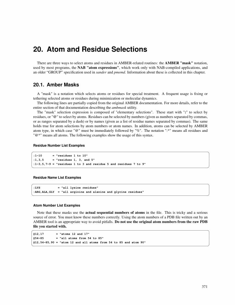
20. Atom and Residue Selections
There are three ways to select atoms and residues in AMBER-related routines: the AMBER "mask" notation,used by most programs, the NAB "atom expressions", which work only with NAB-compiled applications, andan older “GROUP” specification used in sander and pmemd. Information about these is collected in this chapter.
20.1. Amber Masks
A "mask" is a notation which selects atoms or residues for special treatment. A frequent usage is fixing ortethering selected atoms or residues during minimization or molecular dynamics.
The following lines are partially copied from the original AMBER documentation. For more details, refer to theentire section of that documentation describing the ambmask utility.
The "mask" selection expression is composed of "elementary selections". These start with ":" to select byresidues, or "@" to select by atoms. Residues can be selected by numbers (given as numbers separated by commas,or as ranges separated by a dash) or by names (given as a list of residue names separated by commas). The sameholds true for atom selections by atom numbers or atom names. In addition, atoms can be selected by AMBERatom type, in which case "@" must be immediately followed by "%". The notation ":*" means all residues and"@*" means all atoms. The following examples show the usage of this syntax.
Residue Number List Examples :1-10 = "residues 1 to 10"
:1,3,5 = "residues 1, 3, and 5"
:1-3,5,7-9 = "residues 1 to 3 and residue 5 and residues 7 to 9" Residue Name List Examples :LYS = "all lysine residues"
:ARG,ALA,GLY = "all arginine and alanine and glycine residues" Atom Number List Examples
Note that these masks use the actual sequential numbers of atoms in the file. This is tricky and a serioussource of error. You must know these numbers correctly. Using the atom numbers of a PDB file written out by anAMBER tool is an appropriate way to avoid pitfalls. Do not use the original atom numbers from the raw PDBfile you started with. @12,17 = "atoms 12 and 17"
@54-85 = "all atoms from 54 to 85"
@12,54-85,90 = "atom 12 and all atoms from 54 to 85 and atom 90"
371

20. Atom and Residue Selections
Atom Name List Examples @CA = all atoms with the name CA (i.e., all C-alpha atoms)
@CA,C,O,N,H = all atoms with names CA or C or O or N or H
(i.e., the entire protein backbone) Atom Type List Examples
This last mask type is only used by specialists and mentioned here for completeness. It allows the selection ofAMBER atom types and requires detailed knowledge of AMBER force fields. @%CT = all atoms with the force field type CT
(the standard sp3 aliphatic carbon)
@%N*,N3 = all atoms with the force field type N* or N3
(N* is a special sp2 nitrogen, N3 is an sp3 nitrogen) Note that in the above example, N* is actually an atom type. The * is not a wild card meaning "all N-something
types"!
Logical Combinations
The selections above can be combined by various logical operators, including selections like "all atoms withina certain distance from...". The use of such combinations goes beyond this introductory script. Interested usersshould refer to the next section for details.
20.1.1. ambmask
NAME
ambmask - test group input FIND mask (or mask string given in the &cntrl section) and dump the resulting atomselection in a given format
SYNOPSIS
ambmask -p prmtop -c inpcrd -prnlev [0-3] -out [short| pdb| amber] -find [maskstr]
DESCRIPTION
ambmask acts as a filter which takes Amber topology and coordinate "restart" file and applies the "maskstr"selection string (similar syntactically to UCSF Chimera/Midas) to select specific atoms or residues. Residues canbe selected by their numbers or names. Atoms can be selected by numbers, names, or Amber (forcefield) type.Selections are case insensitive. The selected atoms are printed to stdout (by default, in Amber-style PDB format).Atom and residue names and numbers are taken from Amber topology. Beware that selection string works onthose names and not the ones from the original PDB file. If you are not sure how atoms or residues are namedor numbered in the Amber topology, use ambmask with a selection string ":*" (which is the default) to dump thewhole PDB file with corresponding Amber atom/residue names and numbers.
The "maskstr" selection expression is composed of "elementary selections". These start with ":" to select byresidues, or "@" to select by atoms. Residues can be selected by numbers (given as numbers separated bycommas, or as ranges separated by a dash) or by names (given as a list of residue names separated by commas).The same holds true for atom selections by atom numbers or atom names. In addition, atoms can be selected byAmber atom type, in which case "@" must be immediately followed by "%". ":*" means all residues and "@*"means all atoms. The following examples show the usage of this syntax. Square brackets should not be used inactual expressions, they are only used for clarity here:
372

20.1. Amber Masks
:residue numlist [:1-10] [:1,3,5] [:1-3,5,7-9]
:residue namelist [:LYS] [:ARG,ALA,GLY]
@atom numlist [@12,17] [@54-85] [@12,54-85,90]
@atom namelist [@CA] [@CA,C,O,N,H]
@%atom typelist [@%CT] [@%N*,N3]
These "elementary selections" can be combined into more complex selections using binary operators "&" (and)and "|" (or), unary operator "!" (negation), distance binary operators "<:", ">:", "<@", ">@", and parentheses.Spaces around operators are irrelevant. Parentheses have the highest priority, followed by distance operators("<:", ">:", "<@", ">@"), "!" (negation), "&" (and) and "|" (or) in order of descending priority. A wildcard "="in an atom or residue name matches any name starting with a given character (or characters). For example, [:AS=]would match all aspartic acid residues (ASP), and asparagines (ASN); [@H=] would match all atom namesstarting with H (which are effectively all hydrogens). It cannot be used to match the end part of names (such as[:=A]). Some examples of more complex selections follow:
[@C= & !@CA,C]
.. all carbons except backbone alpha and carbonyl carbon
[(:1-3@CA | :5-7@CB)]
.. alpha carbons in residues 1-3 and beta carbons in residues 5-7
[:CYS,ARG & !(:1-10 | @CA,CB)]
.. all CYS and ARG atoms except those which are in residues 1-10 and which are CA or CB
[:* & !@H=] or [!@H=]
.. all heavy atoms (i.e. except hydrogens)
[:5 <@4.5]
.. all atoms within 4.5A from residue 5
[(:1-55 <:3.0) & :WAT]
.. all water molecules within 3A from residues 1-55Compound expressions of the following type are also allowed:
:residue numlist|namelist@atom numlist|namelist|typelist[:1-10@CA] is equivalent to [:1-10 & @CA]
[:LYS@H=] is equivalent to [:LYS & @H=]
OPTIONS
The program needs an Amber topology file and coordinates (restrt format). The filename specified with the -poption is Amber topology, while the filename given with the -c option is a coordinate file. If -p or -c options arenot given, the program expects that files "prmtop" and/or "inpcrd" exist in the current directory, which will betaken as topology and coordinate files correspondingly. If no command line options are given, the program printsthe usage statement.
The option -prnlev specifies how much (debugging) information is printed to stdout. If it is 0, only selectedatoms are printed. More verbose output (which might be useful for debugging purposes) is achieved with highervalues: 1 prints original "maskstr" in its tokenized (with operands enclosed in square brackets) and postfix (orReverse Polish Notation) forms; number of atoms and residues in the topology file and number of selected atomsare also printed to stdout. 2 prints the resulting mask array, which is an array of integer values, with ’1’ representinga selected atom, and ’0’ an unselected one. Value of 3, in addition, prints mask arrays as they are pushed or poppedfrom the stack (this is really only useful for tracing the problems occurring during stack operations). The -prnlevvalues of 0 or 1 should suffice for most uses.
373
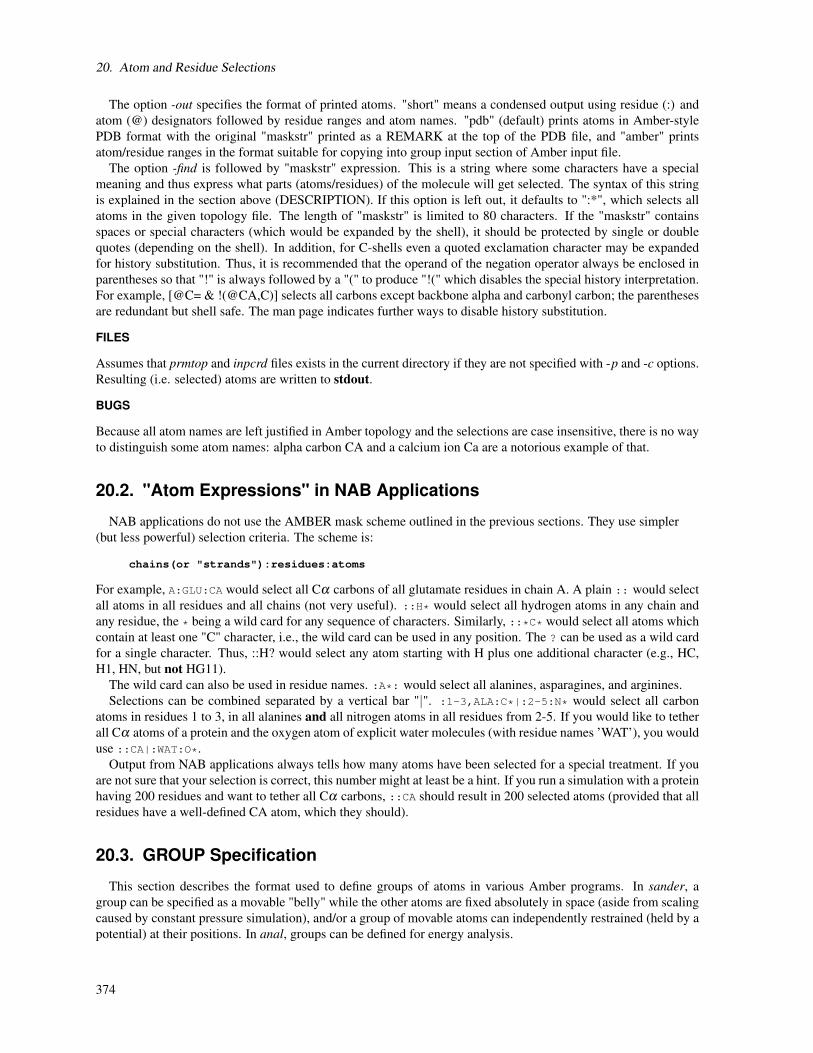
20. Atom and Residue Selections
The option -out specifies the format of printed atoms. "short" means a condensed output using residue (:) andatom (@) designators followed by residue ranges and atom names. "pdb" (default) prints atoms in Amber-stylePDB format with the original "maskstr" printed as a REMARK at the top of the PDB file, and "amber" printsatom/residue ranges in the format suitable for copying into group input section of Amber input file.
The option -find is followed by "maskstr" expression. This is a string where some characters have a specialmeaning and thus express what parts (atoms/residues) of the molecule will get selected. The syntax of this stringis explained in the section above (DESCRIPTION). If this option is left out, it defaults to ":*", which selects allatoms in the given topology file. The length of "maskstr" is limited to 80 characters. If the "maskstr" containsspaces or special characters (which would be expanded by the shell), it should be protected by single or doublequotes (depending on the shell). In addition, for C-shells even a quoted exclamation character may be expandedfor history substitution. Thus, it is recommended that the operand of the negation operator always be enclosed inparentheses so that "!" is always followed by a "(" to produce "!(" which disables the special history interpretation.For example, [@C= & !(@CA,C)] selects all carbons except backbone alpha and carbonyl carbon; the parenthesesare redundant but shell safe. The man page indicates further ways to disable history substitution.
FILES
Assumes that prmtop and inpcrd files exists in the current directory if they are not specified with -p and -c options.Resulting (i.e. selected) atoms are written to stdout.
BUGS
Because all atom names are left justified in Amber topology and the selections are case insensitive, there is no wayto distinguish some atom names: alpha carbon CA and a calcium ion Ca are a notorious example of that.
20.2. "Atom Expressions" in NAB Applications
NAB applications do not use the AMBER mask scheme outlined in the previous sections. They use simpler(but less powerful) selection criteria. The scheme is:
chains(or "strands"):residues:atoms
For example, A:GLU:CA would select all Cα carbons of all glutamate residues in chain A. A plain :: would selectall atoms in all residues and all chains (not very useful). ::H* would select all hydrogen atoms in any chain andany residue, the * being a wild card for any sequence of characters. Similarly, ::*C* would select all atoms whichcontain at least one "C" character, i.e., the wild card can be used in any position. The ? can be used as a wild cardfor a single character. Thus, ::H? would select any atom starting with H plus one additional character (e.g., HC,H1, HN, but not HG11).
The wild card can also be used in residue names. :A*: would select all alanines, asparagines, and arginines.Selections can be combined separated by a vertical bar "|". :1-3,ALA:C*|:2-5:N* would select all carbon
atoms in residues 1 to 3, in all alanines and all nitrogen atoms in all residues from 2-5. If you would like to tetherall Cα atoms of a protein and the oxygen atom of explicit water molecules (with residue names ’WAT’), you woulduse ::CA|:WAT:O*.
Output from NAB applications always tells how many atoms have been selected for a special treatment. If youare not sure that your selection is correct, this number might at least be a hint. If you run a simulation with a proteinhaving 200 residues and want to tether all Cα carbons, ::CA should result in 200 selected atoms (provided that allresidues have a well-defined CA atom, which they should).
20.3. GROUP Specification
This section describes the format used to define groups of atoms in various Amber programs. In sander, agroup can be specified as a movable "belly" while the other atoms are fixed absolutely in space (aside from scalingcaused by constant pressure simulation), and/or a group of movable atoms can independently restrained (held by apotential) at their positions. In anal, groups can be defined for energy analysis.
374

20.3. GROUP Specification
Except in the analysis module where different groups of atoms are considered with different group numbersfor energy decomposition, in all other places the groups of atoms defined are considered as marked atoms to beincluded for certain types of calculations. In the case of constrained minimization or dynamics, the atoms to beconstrained are read as groups with a different weight for each group.
Reading of groups is performed by the routine RGROUP, and you are advised to consult it if there is still someambiguity in the documentation.
Input description:
- 1 - Title format(20a4)
ITITL Group title for identification.
Setting ITITL = ’END’ ends group input.
------------------------------------------------------------------------
- 1A - Weight format(f)
This line is only provided/read when using GROUP input to
define restrained atoms.
WT The harmonic force constants in kcal/mol-A**2 for the group
of atoms for restraining to a reference position.
------------------------------------------------------------------------
- 1B - Control to define the group
KTYPG , (IGRP(I) , JGRP(I) , I = 1,7) format(a,14i)
KTYPG Type of atom selection performed. A molecule can be
defined by using only ’ATOM’ or ’RES’, or part of the
molecule can be defined by ’ATOM’ and part by ’RES’.
’ATOM’ The group is defined in terms of atom numbers. The atom
number list is given in igrp and jgrp.
’RES’ The group is defined in terms of residue numbers. The
residue number list is given in igrp and jgrp.
’FIND’ This control is used to make additional conditions
(apart from the ’ATOM’ and ’RES’ controls) which a given
atom must satisfy to be included in the current group.
The conditions are read in the next section (1C) and are
terminated by a SEARCH card.
Note that the conditions defined by FIND filter any set(s) of atoms
defined by the following ATOM/RES instructions. For example,
-- group input: select main chain atoms --
FIND
* * M *SEARCH
RES 1 999
END
END
’END’ End input for the current group. Followed by either another
group definition (starting again with line 1 above), or by a second
’END’ "card", which terminates all group input.
IGRP(I) , JGRP(I)
The atom or residue pointers. If ktypg .eq. ’ATOM’ all
atoms numbered from igrp(i) to jgrp(i) will be put into
the current group. If ktypg .eq. ’RES’ all atoms in the
residues numbered from igrp(i) to jgrp(i) will be put
into the current group. If igrp(i) = 0 the next control
card is read.
It is not necessary to fill groups according to the
numerical order of the residues. In other words, Group 1
could contain residues 40-95 of a protein, Group 2 could
contain residues 1-40 and Group 3 could contain residues
96-105.
If ktypg .eq. ’RES’, then associating a minus sign with
375

20. Atom and Residue Selections
igrp(i) will cause all residues igrp(i) through jgrp(i)
to be placed in separate groups.
In the analysis modules, all atoms not explicitly defined
as members of a group will be combined as a unit in the
(n + 1) group, where the (n) group in the last defined
group.
------------------------------------------------------------------------
- 1C - Section to read atom characteristics
***** Read only if KTYPG = ’FIND’ *****JGRAPH(I) , JSYMBL(I) , JTREE(I) , JRESNM(I) format(4a)
A series of filter specifications are read. Each filter consists
of four fields (JGRAPH,JSYMBL,JTREE,JRESNM), and each filter is placed
on a separate line. Filter specification is terminated by a line with
JGRAPH = ’SEARCH’. A maximum of 10 filters may be specified for a
single ’FIND’ command.
The union of the filter specifications is applied to the atoms defined
by the following ATOM/RES cards. I.e. if an atom satisfies any of the
filters, it will be included in the current group. Otherwise, it is not
included. For example, to select all non main chain atoms from residues
1 through 999:
-- group input: select non main chain atoms --
FIND
* * S *
* * B *
* * 3 *
* * E *SEARCH
RES 1 999
END
END
’END’ End input for the current group. Followed by either another
The four fields for each filter line are:
JGRAPH(I) The atom name of atom to be included. If this and the
following three characteristics are satisfied the atom is
included in the group. The wild card ’*’ may be used to
to indicate that any atom name will satisfy the search.
JSYMBL(I) Amber atom type of atom to be included. The wild card
’*’ may be used to indicate that any atom type will
satisfy the search.
JTREE(I) The tree name (M, S, B, 3, E) of the atom to be included.
The wild card ’*’ may be used to indicate that any tree
name will satisfy the search.
JRESNM(I) The residue name to which the atom has to belong to be
included in the group. The wild card ’*’ may be used to
indicate that any residue name will satisfy the search.
------------------------------------------------------------------------
Examples:The molecule 18-crown-6 will be used to illustrate the group options. This molecule is composed of six repeating
(-CH2-O-CH2-) units. Let us suppose that one created three residues in the PREP unit: CRA, CRB, CRC. Eachof these is a (-CH2-O-CH2-) moiety and they differ by their dihedral angles. In order to construct 18-crown-6, theresidues CRA, CRB, CRC, CRB, CRC, CRB are linked together during the LINK module with the ring closurebeing between CRA(residue 1) and CRB(residue 6).
Input 1:
Title one
RES 1 5
END
376

20.3. GROUP Specification
Title two
RES 6
END
END
Output 1: Group 1 will contain residues 1 through 5 (CRA, CRB, CRC, CRB, CRC) and Group 2 will containresidue 6 (CRB).
Input 2:
Title one
RES 1 5
END
Title two
ATOM 36 42
END
END
Output 2: Group 1 will contain residues 1 through 5 (CRA, CRB, CRC, CRB, CRC) and Group 2 will containatoms 36 through 42. Coincidentally, atoms 36 through 42 are also all the atoms in residue 6.
Input 3:
Title one
RES -1 6
END
END
Output 3: Six groups will be created; Group 1: CRA, Group 2: CRB,..., Group 6: CRB.Input 4:
Title one
FIND
O2 OS M CRA
SEARCH
RES 1 6
END
END
Output 4: Group 1 will contain those atoms with the atom name ’O2’, atom type ’OS’, tree name ’M’ and residuename ’CRA’.
Input 5:
Title one
FIND
O2 OS * *SEARCH
RES 1 6
END
END
Output 5: Group 1 will contain those atoms with the atom name ’O2’, atom type ’OS’, any tree name and anyresidue name.
Input 6:
Title one
RES 1 3 6 6
END
END
Output 6: One group is created containing residues 1 to 3 and 6. Up to seven ranges of contiguous residues canbe specified per group. (In this case there are two ranges).
377
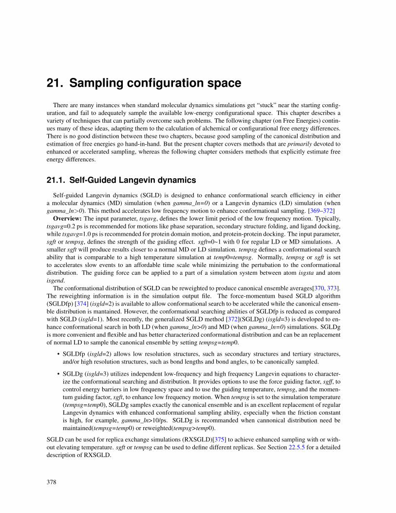
21. Sampling configuration space
There are many instances when standard molecular dynamics simulations get “stuck” near the starting config-uration, and fail to adequately sample the available low-energy configurational space. This chapter describes avariety of techniques that can partially overcome such problems. The following chapter (on Free Energies) contin-ues many of these ideas, adapting them to the calculation of alchemical or configurational free energy differences.There is no good distinction between these two chapters, because good sampling of the canonical distribution andestimation of free energies go hand-in-hand. But the present chapter covers methods that are primarily devoted toenhanced or accelerated sampling, whereas the following chapter considers methods that explicitly estimate freeenergy differences.
21.1. Self-Guided Langevin dynamics
Self-guided Langevin dynamics (SGLD) is designed to enhance conformational search efficiency in eithera molecular dynamics (MD) simulation (when gamma_ln=0) or a Langevin dynamics (LD) simulation (whengamma_ln>0). This method accelerates low frequency motion to enhance conformational sampling. [369–372]
Overview: The input parameter, tsgavg, defines the lower limit period of the low frequency motion. Typically,tsgavg=0.2 ps is recommended for motions like phase separation, secondary structure folding, and ligand docking,while tsgavg=1.0 ps is recommended for protein domain motion, and protein-protein docking. The input parameter,sgft or tempsg, defines the strength of the guiding effect. sgft=0~1 with 0 for regular LD or MD simulations. Asmaller sgft will produce results closer to a normal MD or LD simulation. tempsg defines a conformational searchability that is comparable to a high temperature simulation at temp0=tempsg. Normally, tempsg or sgft is setto accelerates slow events to an affordable time scale while minimizing the pertubation to the conformationaldistribution. The guiding force can be applied to a part of a simulation system between atom isgsta and atomisgend.
The conformational distribution of SGLD can be reweighted to produce canonical ensemble averages[370, 373].The reweighting information is in the simulation output file. The force-momentum based SGLD algorithm(SGLDfp) [374] (isgld=2) is available to allow conformational search to be accelerated while the canonical ensem-ble distribution is mantained. However, the conformational searching abilities of SGLDfp is reduced as comparedwith SGLD (isgld=1). Most recently, the generalized SGLD method [372](SGLDg) (isgld=3) is developed to en-hance conformational search in both LD (when gamma_ln>0) and MD (when gamma_ln=0) simulations. SGLDgis more convenient and flexible and has better characterized conformational distribution and can be an replacementof normal LD to sample the canonical ensemble by setting tempsg=temp0.
• SGLDfp (isgld=2) allows low resolution structures, such as secondary structures and tertiary structures,and/or high resolution structures, such as bond lengths and bond angles, to be canonically sampled.
• SGLDg (isgld=3) utilizes independent low-frequency and high frequency Langevin equations to character-ize the conformational searching and distribution. It provides options to use the force guiding factor, sgff, tocontrol energy barriers in low frequency space and to use the guiding temperature, tempsg, and the momen-tum guiding factor, sgft, to enhance low frequency motion. When tempsg is set to the simulation temperature(tempsg=temp0), SGLDg samples exactly the canonical ensemble and is an excellent replacement of regularLangevin dynamics with enhanced conformational sampling ability, especially when the friction constantis high, for example, gamma_ln>10/ps. SGLDg is recommanded when cannonical distribution need bemaintained(tempsg=temp0) or reweighted(tempsg>temp0).
SGLD can be used for replica exchange simulations (RXSGLD)[375] to achieve enhanced sampling with or with-out elevating temperature. sgft or tempsg can be used to define different replicas. See Section 22.5.5 for a detaileddescription of RXSGLD.
378

21.1. Self-Guided Langevin dynamics
isgld SGLD algorithm index. Default isgld= 0, SGLD is diabled; isgld=1 will turn on SGMD/SGLD methodfor accelerated conformational search; isgld=2 will turn on the SGLDfp method [374] to mantain acanonical ensemble distribution. isgld=3 will enable SGLDg/SGMDg method.
tsgavg Local averaging time (psec) for the guiding force calculation. Default 0.2 psec. A larger value definesslower motion to be enhanced.
sgft Momentum guiding factor. Defines the strength of the guiding effect. Default 1.0 when gamma_ln>0(SGLD), 0.2 when gamma_ln=0 (SGMD), or 0 for SGLDg or 1 for SGMDg (isgld=3). When isgld=1or 2, tempsg>0 will override sgft. When isgld=3 and gamma_ln=0, i.e., SGMDg, sgft represents theguiding friction constant in the unit of 1/ps and should be set to a positive value.
sgff Force guiding factor for SGLDg or SGMDg (isgld=3). sgff is used to scale down low frequencyenergy surface by a factor, (1+sgff ). sgff is suggested to take values between 0 and -0.1, with defaultvalue of 0. sgff is effective for SGMDg (isgld=3 and gamma_ln=0) simulations .
tempsg Target guiding temperature (K). This parameter is redefined since Amber 12 as a conformationalsearch ability which is comparable to a high temperature simulation with temp0=tempsg. For ex-ample, by seting tempsg=500K, a SGMD/SGLD simulation will accelerate conformational search asmuch as rising the simulation temperature to 500K. When isgld=1 or 2, the default is tempsg=0 K.When tempsg=0, the guiding effect will be defined by sgft. tempsg>temp0 will accelerate a confor-mational search and tempsg<temp0 will slow down a conformational search. When isgld=1 or 2,once tempsg is set, sgft will fluctuate to reach the target conformational search ability. When isgld=3(SGLDg), the default is tempsg=temp0, which allows the canonical ensemble will be sampled. Whentempsg<>temp0, the reweighting factor can be found in the SGLD output lines described below.
isgsta The first atom index of SGLD region. Default is 1.
isgend The last atom index of SGLD region. Default is natom.
fixcom Option to remove the net translation of the center of mass. For finite systems it is often more conve-nient to have the center of mass fixed. Default 0 when gamma_ln>0 or 1 when gamma_ln=0. Whenfixcom>0, the center of mass is fixed.
treflf Reference low frequency temperature. Default 0.0. treflf is the low frequency temperature when noguiding force is applied to a simulation system (sgft=0). treflf is required for the weighting factorcalculation in SGMD/SGLD simulation (isgld=1) or for the guiding force calculation in SGMDfp/S-GLDfp simulations (isgld=2). treflf is not needed in SGLDg or SGMDg (isgld=3) simulations. Whentreflf =0, treflf will be estimated during a simulation. An accurate value of treflf can increase theaccuracy in the weighting factor calculation in SGMDfp/SGLDfp simulations.
sgfd Optional high frequency force guiding factor for SGLDfp (isgld=2). Should not be set if conforma-tional distribution in high resolution need be maintained. When not set, its instantaneous value (printedout in simulation output files) fluctuates to maintain high resolution conformational distribution.
The output of SGMD/SGLD simulations contains the following properties related to the enhancement in confor-mational search and reweighting of conformational distribution:
SGLF = SGFT TEMPSG TEMPLF TREFLF FRCLF EPOTLF SGWTSGHF = SGFF SGFD TEMPHF TREFHF FRCHF EPOTHF VIRSG
These quantities are instantaneous values defined as below:SGFT: Momentum guiding factor,SGFF: Force guiding factor. Adjusted in SGLDfp simulations (isgld=2)SGFD: Force dumping factor. Adjusted in SGLDfp simulations (isgld=2)TEMPSG: Guiding temperature.SGWT: Weighting free energy. exp(SGWT) is the weighting factor of current frame.VIRSG: Virial of the guiding force.
379
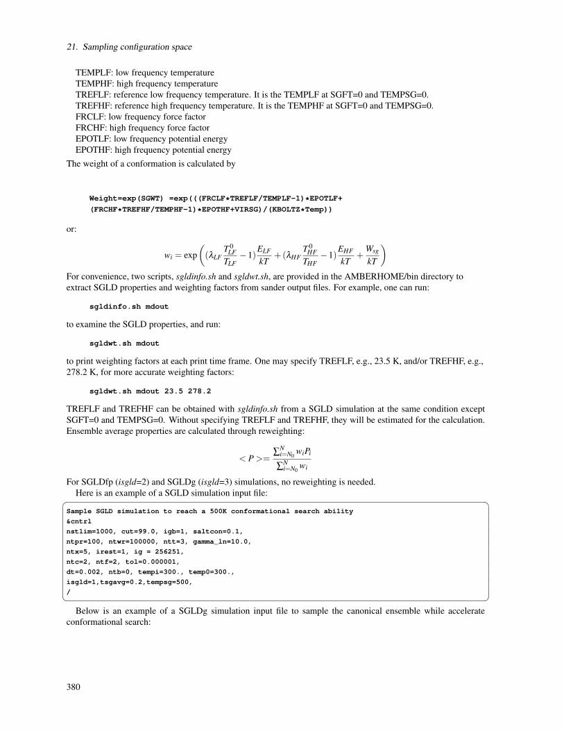
21. Sampling configuration space
TEMPLF: low frequency temperatureTEMPHF: high frequency temperatureTREFLF: reference low frequency temperature. It is the TEMPLF at SGFT=0 and TEMPSG=0.TREFHF: reference high frequency temperature. It is the TEMPHF at SGFT=0 and TEMPSG=0.FRCLF: low frequency force factorFRCHF: high frequency force factorEPOTLF: low frequency potential energyEPOTHF: high frequency potential energy
The weight of a conformation is calculated by
Weight=exp(SGWT) =exp(((FRCLF*TREFLF/TEMPLF-1)*EPOTLF+
(FRCHF*TREFHF/TEMPHF-1)*EPOTHF+VIRSG)/(KBOLTZ*Temp))
or:
wi = exp((λLF
T 0LF
TLF−1)
ELF
kT+(λHF
T 0HF
THF−1)
EHF
kT+
Wsg
kT
)For convenience, two scripts, sgldinfo.sh and sgldwt.sh, are provided in the AMBERHOME/bin directory toextract SGLD properties and weighting factors from sander output files. For example, one can run:
sgldinfo.sh mdout
to examine the SGLD properties, and run:
sgldwt.sh mdout
to print weighting factors at each print time frame. One may specify TREFLF, e.g., 23.5 K, and/or TREFHF, e.g.,278.2 K, for more accurate weighting factors:
sgldwt.sh mdout 23.5 278.2
TREFLF and TREFHF can be obtained with sgldinfo.sh from a SGLD simulation at the same condition exceptSGFT=0 and TEMPSG=0. Without specifying TREFLF and TREFHF, they will be estimated for the calculation.Ensemble average properties are calculated through reweighting:
< P >=∑
Ni=N0
wiPi
∑Ni=N0
wi
For SGLDfp (isgld=2) and SGLDg (isgld=3) simulations, no reweighting is needed.Here is an example of a SGLD simulation input file:
Sample SGLD simulation to reach a 500K conformational search ability
&cntrl
nstlim=1000, cut=99.0, igb=1, saltcon=0.1,
ntpr=100, ntwr=100000, ntt=3, gamma_ln=10.0,
ntx=5, irest=1, ig = 256251,
ntc=2, ntf=2, tol=0.000001,
dt=0.002, ntb=0, tempi=300., temp0=300.,
isgld=1,tsgavg=0.2,tempsg=500,
/ Below is an example of a SGLDg simulation input file to sample the canonical ensemble while accelerate
conformational search:
380

21.2. Accelerated Molecular Dynamics
Sample SGLDg simulation for efficient conformational sampling
&cntrl
nstlim=1000, cut=99.0, igb=1, saltcon=0.1,
ntpr=100, ntwr=100000, ntt=3, gamma_ln=10.0,
ntx=5, irest=1, ig = 256251,
ntc=2, ntf=2, tol=0.000001,
dt=0.002, ntb=0, tempi=300., temp0=300.,
isgld=3,tsgavg=0.2,tempsg=300,sgft=0.5,sgff=-0.1,
/ Below is an example of a SGMDg simulation input file for accelerated conformational search:
Sample SGLDg simulation for efficient conformational sampling
&cntrl
nstlim=1000, cut=99.0, igb=1, saltcon=0.1,
ntpr=100, ntwr=100000, ntt=1, gamma_ln=0.0,
ntx=5, irest=1, ig = 256251,
ntc=2, ntf=2, tol=0.000001,
dt=0.002, ntb=0, tempi=300., temp0=300.,
isgld=3,tsgavg=0.2,tempsg=500,sgft=1,sgff=-0.1,
/ 21.2. Accelerated Molecular Dynamics
21.2.1. Introduction
Many systems of interest in chemistry, physics and biology are characterized by the presence of a number ofmetastable states separated by large barriers. Correctly sampling these systems is challenging for methods based onMolecular Dynamics, Monte Carlo sampling or any other type of dynamic simulation. For most biological systemsof interest, the simulation time is limited to the nanosecond-microsecnd time scale, so simple molecular dynamicscannot be used to adequately explore portions of the energy landscape separated by high barriers from the initialminimum. Furthermore, for most biological molecules, the energy landscape has multiple minima or potentialenergy wells with high free energy barriers, and during a molecular dynamics simulation the system is trapped inone or another local minimum for long periods of simulation time. Consequently, thermodynamics and many otherproperties of interest for large biological systems cannot be simulated directly because of the nonergodic nature ofthe present state of the molecular dynamics methodology for systems with high free energy barriers.
Accelerated Molecular Dynamics (aMD) is a bias potential introduced by the McCammon group at UCSD [376].It is a modification to the potential that in practice reduces the height of local barriers, allowing the calculationto evolve much faster. A number of methods have been suggested to aid this problem, like replica exchange,metadynamics, etc. AMD represents an interesting option as it only requires the evolution of a single copy of thesystem, plus it doesn’t require any previous knowledge of the shape of the potential, i.e. aMD doesn’t requireinformation of where are the barriers, saddle points or even what type of configuration changes are expected ornecessary to traverse through a particular barrier. Moreover, an interesting feature of aMD is that the shape ofthe added potential conserves the underlying shape of the real one, such that minima are maintained as minimaand barriers are preserved as barriers. In result, adding the aMD potential in practice simply modifies the relationbetween energy differences, so the distribution of sampling of different structures is still related to the originalpotential distribution and can be recovered exactly by reweighing.
The aMD modification of the potential is defined by the following equation:
V(r)∗=V (r)+∆V (r) (21.1)
∆V (r) =(E p−V (r))2
(αP+E p−V (r))+
(Ed−V d(r))2
(αD+Ed−V d(r))(21.2)
381

21. Sampling configuration space
where V (r) is the normal potential and V d(r) is the normal torsion potential. Ep and Ed are average potentialand dihedral energies that serve as a reference energy from which to compare the present position of the calculationand therefore the relationship to the boosting factor to be applied. The terms αP and αD are factors that determineinversely the strength with which the boost is applied. For large values of alpha, the potential felt at any pointwill essentially be the same as the true potential For values of alpha close to zero, the potential felt becomesconstant, in this limit, the sampling becomes a random walk. The amount of boost felt at a particular point inthe calculation, therefore, depends on the present value of the potential and dihedral energy, which is in directcorrelation to how low in the energy surface the configuration is positioned at that moment. The boosting potentialwill be proportionally bigger for deeper regions of the potential energy surface, while it will be smaller for higherpoints, which in result conserves the underlying shape of the potential, as previously mentioned.
AMD has been applied to a vast diversity of interesting problems [377–381]. We have recently applied theimplementation of aMD in Amber to the Bovine Pancreatic Trypsin Inhibitor and compared with an unbiasedmillisecond MD simulation, showing aMD is able to recover the right population distribution and shows excellentagreement with the MD simulation as with experimental data [380].
21.2.2. AMD implementation in Amber
AMD has been implemented in both sander and pmemd by Romelia Salomon-Ferrer. The implementationincludes the possibility of boosting independently only the torsional terms of the potential (iamd=2) or the wholepotential at once (iamd=1). It also allows the possibility to boost the whole potential with an extra boost to thetorsions(iamd=3). All the information generated by aMD, necessary for reweighing is stored at each step into avector which is flushed to a log file (amd.log by default) every time the coordinates are written to disk, i.e. everyntwx steps. This is done for performance reasons, since writing to disk is always time consuming and it is notadvisable to do it every step. The name of the log file can be set to a user defined name by using the commandline option -amdlog when running Amber. Our present implementation also allows the user to delay (or lag) theboosting a number of steps, i.e. only boost with a particular frequency defined by the variable amdlag. Additionalparameters are specified by the following variables: EthreshD (Ed), alphaD (αD), EthreshP (Ep) and alphaP (αP).
AMD output is saved the amd.log this file contains all the information needed for reweighting the results obtainedto recover the unperturbed distributions. The amd.log file gets written with the same frequency at which theconfigurations are saved to disk in the trajectory file (mdcrd). Each line corresponds to the information of acorresponding snapshot being saved on the mdcrd file. Regardless of what iamd value is used, the number ofcolumns in the amd.log file are always the same, they just have 0 or 1 (correspondingly) if no boost is being addedto dihedral or total energy
The amd.log file has the following header:
#All energy terms stored in units of kcal/mol
#ntwx,total_nstep,Unboosted-Potential-Energy,Unboosted-Dihedral-Energy,Total-Force-Weight,
Dihedral-Force-Weight,Boost-Energy-Potential,Boost-Energy-Dihedral
The description for the main columns is as follows:
• Unboosted-Potential-Energy: Total Potential Energy without boost added, kcal/mol.
• Unboosted-Dihedral-Energy: dihedral energy without boost added, kcal,mol.
• Total-Force-Weight: The force scaling factor calculated from the boost to the Total Potential Energy
• Dihedral-Force-Weight: The dihedral force scaling factor from dihedral boost
• Boost-Energy-Potential: The boost energy in kcal/mol
• Boost-Energy-Dihedral: The dihedral boost energy in kcal/mol
IMPORTANT NOTE: Before Amber 14 the boost energy for the dihedral and total potential energy (last twocolumns) was given in units of kT. This decision was made at the beginning with the idea that the user could readand use these values directly for reweighting without any further work, but later it we decided it was much betterand more consistent to have all energy output in kcal/mol as the rest of AMBER’s energy output. As of AMBER14, the last two columns of the amd.log file as given in units of kcal/mol.
382

21.2. Accelerated Molecular Dynamics
Reweighting
For reweighting aMD results we would like to add the link to a great tutorial(http://mccammon.ucsd.edu/computing/amdReweighting/) which also provides a small python script to perfomthe reweighting. The script is compatible with the newer versions of AMBER, and can be used to reweight 1Dand 2D distributions. A simple C code is also provided in the aMD tutorial that performs reweighting based onthe Kernel Density Estimation algorithm. This algorithm also performs very well and reduces the amount of noisewithout using a truncated expression for the exponential and can be used as an alternative for reweighting. Toextract the energies from the amd.log file into a file, weights.dat, to use with this script, something like thefollowing could be done:
# Column 1: dV in units of kbT; column 2: timestep; column 3: dV in units of kcal/mol
# For AMBER14: # awk ’NR%1==0’ amd.log | awk ’print ($8+$7)/(0.001987*300)
" " $2 " " ($8+$7)’ > weights.dat
# For AMBER12: # awk ’NR%1==0’ amd.log | awk ’print ($8+$7)" " $3
" " ($8+$7)*(0.001987*300)’ > weights.dat
For reweighting a 2D distribution, for instance a Phi Psi distribution, you would need to extract the values for Phiand Psi for each frame in the mdcrd file using AmberTools and generate the file Phi_Psi file and then use thepython tool provided in the website to get the reweighted surface.
python PyReweighting-2D.py -input Phi_Psi -Emax 100 -discX 6 -discY 6
-job amdweight_MC -order 10 -weight weights.dat | tee -a reweight_variable.log
For reweighting using a Maclaurin series expansion as an approximation for the exponential weight.
21.2.3. Preparing a system for aMD
As mentioned before, running aMD requires the definition of few parameters. AMD parameters are determinedbased on previous knowledge of the system, which is easily acquirable by a short regular MD simulation, fromwhich the average values of the potential and torsion energy can be estimated. From there, a given amount ofenergy per degree of freedom is added those values, in the form of multiples of alpha, setting the values of Ep andEd to be used. The following example should help clarify this procedure.
Average Dihedral : 611.5376 (based on MD simulations)
Average EPtot : -53155.3104 (based on MD simulations)
total ATOMS=16950
protein residues=64
For the dihedral potential:
Approximate energy contribution per degree of freedom.
3.5*64= 224 The value of 3.5 kcal/mol/residue seems to work well
alphaD = (1/5)*224 = 45 The value of .2 seems to work well
EthreshD = 224+611 = 835
For the total potential
alphaP = 16950*(1/5)=3390
For a lower boost you can also use a value between 0.15-0.19 instead of 0.20 (0.16 works well)
EthreshP = -53155.3104 + 3390 = -49765.3104
With these parameters, the aMD parameters in the input file should then be set to
iamd=3,EthreshD=835,alphaD=45,EthreshP=-49765,alphaP=3390,
383

21. Sampling configuration space
For a higher acceleration it is common to simply add to Eb(dih) multiples of alpha. In this example, one level of acceleration higher than the base for the diedral potential would be defined by:
iamd=3,EthreshD=880,alphaD=45,EthreshP=-49765,alphaP=3390,
Two levels higher would be then defined by:
iamd=3,EthreshD=925,alphaD=45,EthreshP=-49765,
After the aMD parameters to be used are defined, an MD run with aMD can be set using those parameters. De-pending on the progress of the simulation, a higher boost can be applied as specified in the above example.
21.2.4. Sample input file for aMD
An example of an input file would be the following:
AVP dt=2.0fs with SHAKE, NPT aMD boost pot and dih
&cntrl
imin=0, irest=1, ntx=5,
dt=0.002, ntc=2, ntf=2, tol=0.000001,iwrap=1,
ntb=2, cut=12.0, ntp=1,igb=0,ntwprt = 3381,ioutfm = 1,
ntt=3, temp0=310.0, gamma_ln=1.0, ig=-1,
ntpr=1000, ntwx=1000, ntwr=2000000, nstlim=2000000,
iamd=3,EthreshD=835,
alphaD=45,EthreshP=-49765,
alphaP=3390,
/
&ewald
dsum_tol=0.000001,
/
21.2.5. Further information
Test cases have been included into the distribution of Amber, also a tutorial based on a study we performed onBPTI [380], showing the power of aMD and its validation versus a millisecond run on the same system performedon Anton is now present on the Amber website. We encourage the user to read the paper, as well as follow thetutorial for more information.
21.3. Gaussian Accelerated Molecular Dynamics
Gaussian Accelerated Molecular Dynamics (GaMD) is a biomolecular enhanced sampling method that worksby adding a harmonic boost potential to smoothen the system potential energy surface. The boost potential fol-lows Gaussian distribution, which allows for accurate reweighting using cumulant expansion to the second order.GaMD has been demonstrated on simulations of alanine dipeptide, chignolin folding and ligand binding to theT4-lysozyme [382]. GaMD enables unconstrained enhanced sampling of these biomolecules without the need toset predefined reaction coordinates. Furthermore, the free energy profiles obtained from reweighting of the GaMDsimulations help identify distinct low energy states of the biomolecules and characterize the protein folding andligand binding pathways quantitatively.
The basic theory of GaMD can be found in References [382, 383], or at http://gamd.ucsd.edu.GaMD has been implemented in pmemd, both the serial and parallel versions on CPU (pmemd and pmemd.MPI)
and GPU (pmemd.cuda and pmemd.cuda.MPI) by Yinglong Miao. Note that GaMD is not available in Sander.Similar to aMD, GaMD provides options to add only the total potential boost (igamd=1), only dihedral potentialboost (igamd=2), or the dual potential boost (igamd=3). The dual-boost simulation generally provides higheracceleration than the other two types of simulations for enhanced sampling. The simulation parameters compriseof the threshold energy values and the effective harmonic force constants, and for the total and dihedral potentialboost, respectively. All the information generated by GaMD, necessary for reweighing is stored at each step into avector which is flushed to a log file (gamd.log by default) every time the coordinates are written to disk, i.e. every
384
21.3. Gaussian Accelerated Molecular Dynamics
ntwx steps. The name of the log file can be set to a user defined name by using the command line option -gamdlogwhen running Amber. Additional parameters are specified by the following variables:
igamd Flag to apply boost potential
= 0 (default) no boost is applied
= 1 boost on the total potential energy only
= 2 boost on the dihedral energy only
= 3 dual boost on both dihedral and total potential energy
iE Flag to set the threshold energy E
= 1 (default) set the threshold energy to the lower bound E = Vmax
= 2 set the threshold energy to the upper bound E =Vmin +(Vmax−Vmin)/k0
ntcmdprep The number of preparation conventional molecular dynamics steps. This is used for system equilibra-tion and the potential energies are not collected for calculating their statistics. The default is 200,000for a simulation with 2 fs timestep.
ntcmd The number of initial conventional molecular dynamics simulation steps. Potential energies are col-lected between ntcmdprep and ntcmd to calculate their maximum, minimum, average and standarddeviation (Vmax,Vmin,Vavg, σV ). The default is 1,000,000 for a simulation with 2 fs timestep.
ntebprep The number of preparation biasing molecular dynamics simulation steps. This is used for systemequilibration after adding the boost potential and the potential statistics (Vmax,Vmin,Vavg, σV ) are notupdated during these steps. The default is 200,000 for a simulation with 2 fs timestep.
nteb The number of biasing molecular dynamics simulation steps. Potential statistics (Vmax, Vmin, Vavg,σvV) are updated between the ntebprep and nteb steps and used to calculate the GaMD acceleration pa-rameters, particularly E and k0. The default is 1,000,000 for a simulation with 2 fs timestep. A greatervalue may be needed to ensure that the potential statistics and GaMD acceleration parameters leveloff before running production simulation between the nteb and nstlim (total simulation length) steps.Moreover, nteb can be set to nstlim, by which the potential statistics and GaMD acceleration parame-ters are updated adaptively throughout the simulation. This in some cases provides more appropriateacceleration.
ntave The number of simulation steps used to calculate the average and standard deviation of potentialenergies. This variable has already been used in Amber. The default is set to 50,000 for GaMDsimulations. It is recommended to be updated as about 4 times of the total number of atoms in thesystem. Note that ntcmd and nteb need to be multiples of ntave.
sigma0P The upper limit of the standard deviation of the total potential boost that allows for accurate reweight-ing if igamd is set to 1 or 3. The default is 6.0 (unit: kcal/mol).
sigma0D The upper limit of the standard deviation of the dihedral potential boost that allows for accuratereweighting if igamd is set to 2 or 3. The default is 6.0 (unit: kcal/mol).
irest_gamd Flag to restart GaMD simulation
= 0 (default) new simulation. A file "gamd-restart.dat" that stores the maximum, minimum, averageand standard deviation of the dihedral and/or total potential energies (depending on the igamdflag) will be saved automatically after GaMD equilibration stage.
= 1 restart simulation (ntcmd is set to 0 in this case). The "gamd-restart.dat" file will be read forrestart.
The GaMD algorithm is summarized as follows:
385
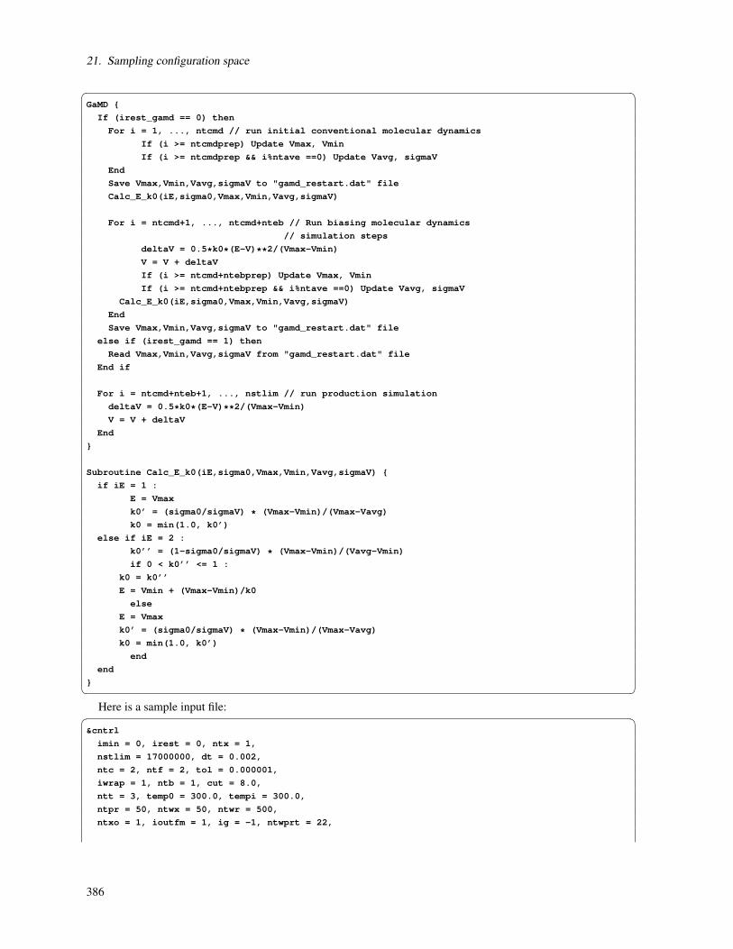
21. Sampling configuration space
GaMD
If (irest_gamd == 0) then
For i = 1, ..., ntcmd // run initial conventional molecular dynamics
If (i >= ntcmdprep) Update Vmax, Vmin
If (i >= ntcmdprep && i%ntave ==0) Update Vavg, sigmaV
End
Save Vmax,Vmin,Vavg,sigmaV to "gamd_restart.dat" file
Calc_E_k0(iE,sigma0,Vmax,Vmin,Vavg,sigmaV)
For i = ntcmd+1, ..., ntcmd+nteb // Run biasing molecular dynamics
// simulation steps
deltaV = 0.5*k0*(E-V)**2/(Vmax-Vmin)
V = V + deltaV
If (i >= ntcmd+ntebprep) Update Vmax, Vmin
If (i >= ntcmd+ntebprep && i%ntave ==0) Update Vavg, sigmaV
Calc_E_k0(iE,sigma0,Vmax,Vmin,Vavg,sigmaV)
End
Save Vmax,Vmin,Vavg,sigmaV to "gamd_restart.dat" file
else if (irest_gamd == 1) then
Read Vmax,Vmin,Vavg,sigmaV from "gamd_restart.dat" file
End if
For i = ntcmd+nteb+1, ..., nstlim // run production simulation
deltaV = 0.5*k0*(E-V)**2/(Vmax-Vmin)
V = V + deltaV
End
Subroutine Calc_E_k0(iE,sigma0,Vmax,Vmin,Vavg,sigmaV)
if iE = 1 :
E = Vmax
k0’ = (sigma0/sigmaV) * (Vmax-Vmin)/(Vmax-Vavg)
k0 = min(1.0, k0’)
else if iE = 2 :
k0’’ = (1-sigma0/sigmaV) * (Vmax-Vmin)/(Vavg-Vmin)
if 0 < k0’’ <= 1 :
k0 = k0’’
E = Vmin + (Vmax-Vmin)/k0
else
E = Vmax
k0’ = (sigma0/sigmaV) * (Vmax-Vmin)/(Vmax-Vavg)
k0 = min(1.0, k0’)
end
end
Here is a sample input file:
&cntrl
imin = 0, irest = 0, ntx = 1,
nstlim = 17000000, dt = 0.002,
ntc = 2, ntf = 2, tol = 0.000001,
iwrap = 1, ntb = 1, cut = 8.0,
ntt = 3, temp0 = 300.0, tempi = 300.0,
ntpr = 50, ntwx = 50, ntwr = 500,
ntxo = 1, ioutfm = 1, ig = -1, ntwprt = 22,
386

21.4. Targeted MD
igamd = 3, iE = 1, irest_gamd = 0,
ntcmd = 1000000, nteb = 1000000, ntave = 50000,
ntcmdprep = 200000, ntebprep = 200000,
sigma0P = 6.0, sigma0D = 6.0,
&end Reweighting analysis of GaMD simulations is similar to that of previous aMD simulations, except that the
amd.log file name needs to be replaced by gamd.log. Test cases have been included into the distribution of Amber,also a tutorial based on a study we performed on alanine dipeptide [382], demonstrating the usage of GaMDon unconstrained enhanced sampling and free energy calculation of biomolecules is now present on the Amberwebsite. We encourage the user to read the paper, as well as follow the tutorial for more information. The latestupdates and simulation tips of GaMD can be also found at http://gamd.ucsd.edu.
21.4. Targeted MD
The targeted MD option adds an additional term to the energy function based on the mass-weighted root meansquare deviation of a set of atoms in the current structure compared to a reference structure. The referencestructure is specified using the -ref flag in the same manner as is used for Cartesian coordinate restraints(NTR=1). Targeted MD can be used with or without positional restraints. If positional restraints are not applied(ntr=0), sander performs a best-fit of the reference structure to the simulation structure based on selection intgtfitmask and calculates the RMSD for the atoms selected by tgtrmsmask. The two masks can be identical ordifferent. This way, fitting to one part of the structure but calculating the RMSD (and thus restraint force) foranother part of the structure is possible. If targeted MD is used in conjunction with positional restraints (ntr=1),only tgtrmsmask should be given in the control input because the molecule is ’fitted’ implicitly by applyingpositional restraints to atoms specified in restraintmask.The energy term has the form:
E = 0.5 * TGTMDFRC * NATTGTRMS * (RMSD-TGTRMSD)**2
The energy will be added to the RESTRAINT term. Note that the energy is weighted by the number of atomsthat were specified in the tgtrmsmask (NATTGTRMS). The RMSD is the root mean square deviation and is massweighted. The force constant is defined using the tgtmdfrc variable (see below). This option can be used withmolecular dynamics or minimization. When targeted MD is used, sander will print the current values for theactual and target RMSD to the energy summary in the output file.
itgtmd
= 0 no targeted MD (default)
= 1 use targeted MD
= 2 use targeted MD to multiple targets (Multiply-targeted MD, or MTMD, see next section below)
tgtrmsd Value of the target RMSD. The default value is 0. This value can be changed during the simulation byusing the weight change option.
tgtmdfrc This is the force constant for targeted MD. The default value is 0, which will result in no penalty forstructure deviations regardless of the RMSD value. Note that this value can be negative, which wouldforce the coordinates AWAY from the reference structure.
tgtfitmask Define the atoms that will be used for the rms superposition between the current structure and thereference structure. Syntax is in Chapter 20.1.1.
tgtrmsmask Define the atoms that will be used for the rms difference calculation (and hence the restraint force),as outlined above. Syntax is in Chapter 20.1.1.
387
21. Sampling configuration space
One can imagine many uses for this option, but a few things should be kept in mind. In this implementation oftargeted MD, there is currently only one reference coordinate set, so there is no way to force the coordinates to anyspecific structure other than the one reference. To move a structure toward a reference coordinate set, one mightuse an initial tgtrmsd value corresponding to the actual RMSD between the input and reference (inpcrd and refc).Then the weight change option could be used to decrease this value to 0 during the simulation. To move a structureaway from the reference, one can increase tgtrmsd to values larger than zero. The minimum for this energy termwill then be at structures with an RMSD value that matches tgtrmsd. Keep in mind that many different structuresmay have similar RMSD values to the reference, and therefore one cannot be sure that increasing tgtrmsd to agiven value will result in a particular structure that has that RMSD value. In this case it is probably wiser to usethe final structure, rather than the initial structure, as the reference coordinate set, and decrease tgtrmsd during thesimulation. To address this, multiply-targeted MD is now available in Amber (sander only), and is described in thenext section. As an additional note, a negative force constant tgtmdfrc can be used, but this can cause problemssince the energy will continue to decrease as the RMSD to the reference increases.
Also keep in mind that phase space for molecular systems can be quite complex, and this method does notguarantee that a low energy path between initial and target structures will be followed. It is possible for thesimulation to become unstable if the restraint energies become too large if a low-energy path between a simulatedstructure and the reference is not accessible.
Note also that the input and reference coordinates are expected to match the prmtop file and have atoms in thesame sequence. No provision is made for symmetry; rotation of a methyl group by 120° would result in a nonzeroRMSD value.
21.5. Multiply-Targeted MD (MTMD)
In Amber (sander only), the user may perform targeted MD calculations using multiple reference structures.Each reference may have its own associated target RMSD value and force constant, each of which can evolveindependently in time. Additionally, the masks for each defined target may differ, and targeting to any givenreference structure can be activated for some or part of the simulation. The energy term for MTMD is simply thesum of the energies that would be calculated for the molecule calculated relative to each target given the targetRMSD and force constant for that target. The energy will then be added to the RESTRAINT term.
To use MTMD, the MTMD input file is specified using the -mtmd flag in the command line arguments forsander. The MTMD input file will contain one instance of the tgt namelist (“&tgt”) for each reference structureused. The user may specify any number of reference structures.
21.5.1. Variables in the &tgt namelist:
refin The file name of the reference structure used. The input and reference coordinates are expected tomatch the prmtop file and have atoms in the same sequence. Default for refin is ”, no referencestructure given.
mtmdform If MTMDFORM > 0, then the reference coordinate file is formatted. Otherwise, the reference coor-dinate file is an unformatted (binary) file. Default for MTMDFORM is the value assigned to MTMD-FORM in the most recent namelist where MTMDFORM was specified. If MTMDFORM has not beenspecified in any namelist, it defaults to 1.
mtmdstep1, mtmdstep2 Targeted MD for this structure is run for steps/iterations MTMDSTEP1 through MTMD-STEP2. If MTMDSTEP2 = 0, then TMD will be run through the end of the run, and the values ofthe target RMSD and the force constant will not change with time. Note that the first step/iterationis considered step 0. Defaults for MTMDSTEP1 and MTMDSTEP2 are the values assigned to themin the most recent namelist where MTMDSTEP1 and MTMDSTEP2 were specified. If MTMDSTEP1and MTMDSTEP2 have not been specified in any namelist, they default to 0.
mtmdvari If MTMDVARI > 0, then the force constant and target RMSD will vary with step number. Oth-erwise, they are constant throughout the run. If MTMDVARI >0, then the values MTMDSTEP2,
388

21.6. Nudged elastic band calculations
MTMDRMSD2, and MTMDFORCE2 must be specified (see below). Default for MTMDVARI isthe value assigned to MTMDVARI in the most recent namelist where MTMDVARI was specified. IfMTMDVARI has not been specified in any namelist, it defaults to 0.
mtmdrmsd, mtmdrmsd2 The target RMSD for this reference. If MTMDVARI >0, then the value of MTMDRMSDwill vary between MTMDSTEP1 and MTMDSTEP2, so that, e.g. MTMDRMSD(MTMDSTEP1) =MTMDRMSD and MTMDRMSD(MTMDSTEP2) = MTMDRMSD2. Defaults for MTMDRMSD andMTMDRMSD2 are the values assigned to them in the most recent namelist where MTMDRMSD andMTMDRMSD2 were specified. If MTMDRMSD and MTMDRMSD2 have not been specified in anynamelist, they default to 0.0.
mtmdforce, mtmdforce2 The force constant for this reference. If MTMDVARI >0, then the value ofMTMDFORCE will vary between MTMDSTEP1 and MTMDSTEP2, so that, e.g. MTMD-FORCE(MTMDSTEP1) = MTMDFORCE and MTMDFORCE(MTMDSTEP2) = MTMDFORCE2.Defaults for MTMDFORCE and MTMDFORCE2 are the values assigned to them in the most recentnamelist where MTMDFORCE and MTMDFORCE2 were specified. If MTMDFORCE and MTMD-FORCE2 have not been specified in any namelist, they default to 0.0.
mtmdninc If MTMDVARI >0 and MTMDNINC > 0, then the changes in the values of of MTMDRMSD andMTMDFORCE are applied as a step function, with NINC steps/iterations between each change in thetarget values. If MTMDNINC = 0, the change is effected continuously (at every step). Default forMTMDNINC is the value assigned to MTMDNINC in the most recent namelist where MTMDNINCwas specified. If MTMDNINC has not been specified in any namelist, it defaults to 0.
mtmdmult If MTMDMULT=0, and the values of MTMDFORCE changes with step number, then the changesin the force constant will be linearly interpolated from MTMDFORCE→MTMDFORCE2 as the stepnumber changes. If MTMDMULT=1 and the force constant is changing with step number, then thechanges in the force constant will be effected by a series of multiplicative scalings, using a singlefactor, R, for all scalings. i.e.
MTMDFORCE2 = R**INCREMENTS * MTMDFORCE
INCREMENTS is the number of times the target value changes, which is determined by MTMD-STEP1, MTMDSTEP2, and MTMDNINC. Default for MTMDMULT is the value assigned to MT-MDMULT in the most recent namelist where MTMDMULT was specified. If MTMDMULT has notbeen specified in any namelist, it defaults to 0.
mtmdmask Define the atoms that will be used for both the rms superposition between the current structure andthe reference structure and the rms difference calculation (and hence the restraint force), as outlinedabove. Syntax is in Chapter 20.1.1.Default for MTMDMASK is the value assigned to MTMDMASK inthe most recent namelist where MTMDMASK was specified. If MTMDMASK has not been specified inany namelist, it defaults to ’*’, use all atoms in the fit and force calculations. \
Namelist &tgt is read for each reference structure. Input ends when a namelist statement with refin = ” (or refinnot specified) is found. Note that comments can precede or follow any namelist statement, allowing comments andreference definitions to be freely mixed.
21.6. Nudged elastic band calculations
21.6.1. Background
In the nudged elastic band method (NEB),[384, 385] the path for a conformational change is approximated witha series of images of the molecule describing the path. Minimization, with the images at the endpoints fixed inspace, of the total system energy provides a minimum energy path. Each image in-between is connected to theprevious and next image by "springs" along the path that serve to keep each image from sliding down the energylandscape onto adjacent images. NEB is derived from the plain elastic band method, pioneered by Elber and
389

21. Sampling configuration space
Karplus,[386] which added the spring forces to the potential of energy surface and minimized the energy of thesystem. The plain elastic band method found low energy paths, but tended to cut corners in the energy landscape.NEB prevents corner cutting by truncating the spring forces in directions perpendicular to the tangent of the path.Furthermore, the forces from the molecular potential are truncated along the path, so that images remain evenlyspaced along the path. This leads to:
F = F⊥+F‖
F⊥ = −∇V (P)+((∇V (P) · τ)τ (21.3)
F‖ = [(ki+1|Pi+1−Pi|− ki|Pi−Pi−1) · τ]τ
where, if N is the number of atoms per image, F is the force on image i, Pi is the 3N dimensional position vectorof image i, ki is the spring constant between image i−1 and image i, V is the potential described by the force field,and τ is the 3N dimensional tangent unit vector that describes the path.
The simplest definition of τ is:
τ = (Pi−Pi−1)/|Pi−Pi−1| (21.4)
This definition leads to instability in the path caused by kinks that occur where the magnitude of F‖ is much largerthan the magnitude of F⊥. A more stable tangent definition was derived to prevent kinks in the path that dependsupon the energies, E, of adjacent images.[387] The spring constants can be the same between all images or theycan be scaled to move the images closer together in the regions of transition states:[388]
I f (Ei > Ere f ) then ki = kmax−∆k(Emax−Ei)/(Emax−Ere f )
otherwise ki = kmax−∆k (21.5)
Here Emax is the highest energy for an image along the path, Ere f is the energy of the higher energy endpoint,and kmax and ∆k are parameters with units of force per length. Because the spring force applies only in directionsalong the path and because the potential of the energy surface is zeroed along the path, the calculation is relativelyinsensitive to the magnitude of the spring constants. Care must be taken, however, to select a spring constant thatdoes not result in higher frequency motions than those found in the system of interest.[389] At each step, beforecalculating the spring forces that compose F‖, each image’s neighbor is rotated and translated onto itself to findthe RMSD minimum, based on a subset of the system’s atoms which the user can define. In this way, each imageremains a continuous MD simulation, and the communication of coordinates can be greatly reduced.
Energy minimization of the path is complicated by the fact that the forces are truncated according to the tangentdirection, making it impossible to define a Lagrangian.[389] Conjugate gradient minimization, therefore, cannotbe used to find the minimum energy path. An algorithm for quenched molecular dynamics has been used to findthe minimum.[385] With this method, the component of the velocity parallel to the force is kept, but perpendicularcomponents are scaled:
I f (v · f > 0) then v = (v · f)fotherwise v = x(v · f)f (21.6)
where f is the 3N-dimensional unit force vector, v is the 3N-dimensional velocity vector, and x is a scaling fac-tor less than one. Recently, a super-linear minimization method was described using an adopted basis Newton-Raphson minimizer.[389]
A partial NEB (PNEB) implementation is available, and is the only form of NEB that is currently supported[390]. This implementation allows the NEB method to be applied to a user defined subset of the system of interest.It requires users to define the part of the system to apply NEB force decoupling to, as well as the part of the systemto RMS fit neighboring images to, to remove rotational and translational motion. This allows NEB to be usedefficiently in large systems where a local transition is desired, or in explicitly solvated systems.
390

21.6. Nudged elastic band calculations
As with the previous implementation of NEB in sander.MPI [391], minimization of the system energies alongthe lowest potential energy path is achieved by simulated annealing. This requires no hypothesis for a starting path,but does require careful judgment of the temperature and length of time required to populate the minimum energypath. The initial coordinates can have multiple copies of the structure superimposed on the start and endpoints.When adjacent structures are superimposed, the tangent, τ is 0 in every direction. This case is explicitly handledso that the calculation is stable.
21.6.2. Preparing input files for NEB
The NEB capability is implemented inside sander.MPI and uses the multisander functionality. Input prmtop andinpcrd files for NEB should be generated using Leap. For NEB you need as a minimum a prmtop for a singleimage of your molecule and two inpcrd files representing each end of the pathway.
The following are some notes for preparing NEB input files:
1. Always check that the prmtop files generated for the endpoint coordinates are identical. This can be done bydiffing the files. One prmtop must be used to describe both endpoints’ inpcrd files.
2. If you have intermediate structures along the path, you must make sure the prmtop is appropriate for thisstructure as well.
3. The endpoint images serve as coordinate reference points, and the first and last images remain fixed incoordinate and energy space along the path. No simulation is performed on these during NEB optimization,so they must initially be well minimized to prevent the rest of the images from migrating to a local minimumbefore the conformational transition occurs. Take this into consideration when choosing the number ofimages to connect along the path.
Multisander requires a groupfile input, where each line of the groupfile is the sander command for each individualimage’s MD simulation. Multiple copies of each endpoint image are used for the initial simulation. If intermediatesare available and the user wishes to include them, they should be added sequentially in between the endpointconformations in the order in which these structures are thought to appear along the transition path.
Notes for running NEB using multisander:
1. The number of CPUs specified must be a multiple of the number of images. You can run this on a standarddesktop computer, but it will generally be more efficient to run it on a minimum of one processor per image.
2. If the user has access to parallel computing resources, multiple processors per image may be used. Carefulbenchmarking should be done to gauge the best balance between computational efficiency in calculating thedynamics of each image and slowdown caused by communications overhead at each step.
21.6.3. Input Variables
ineb Flag for nudged elastic band. A value of 0 (default) means that no nudged elastic band will be used.A value of 1 means that a NEB simulation is being performed.
tgtfitmask Flag which sets atoms to RMS fit each image’s neighbor to itself. This must not include solvent,which, due to diffusion, overlapping proves impossible. The more atoms you choose, the more com-munication has to be done by each bead. Syntax for this is here: 20.1.1
tgtrmsmask Flag which sets atoms to decouple NEB forces for PNEB. This can be set to all atoms of the solute,or a subset of atoms which best describes the area of the system which undergoes the conformationalchange you wish to see. Syntax for this is here: 20.1.1
skmax Spring constant or kmax from above (100 by default).
skmin If skmin = skmax, a fixed spring constant is used. Otherwise, skmin is taken from above for scaledspring constants (50 by default).
391

21. Sampling configuration space
tmode If 1 (default), use the revised tangent definition that prevents kinks. For any other value, use the simple(original) tangent definition.
vv If this is 1, use the quenched velocity Verlet minimization; otherwise, do not.
vfac Scaling factor for quenched velocity Verlet algorithm. (0.0 by default).
Sample input file for running initial heating along the path.Below is an example input file that can be used to perform the initial heating step of a NEB run. Note that the
input and topology files must be identical for each bead; the names of the output, trajectory, restart and info filesshould not be the same between beads.
Alanine NEB initial MD with small K
&cntrl
imin = 0, irest = 0,
ntc=1, ntf=1,
ntpr=1, ntwx=500,
ntb = 0, cut = 999.0, rgbmax=999.0,
igb = 1, saltcon=0.2,
nstlim = 40000, nscm=0,
dt = 0.0005, ig=42,
ntt = 3, gamma_ln=1000.0,
tempi=0.0, temp0=300.0,
tgtfitmask=":1,2,3",
tgtrmsmask=":1,2,3@N,CA,C",
ineb = 1,skmin = 10,skmax = 10,
nmropt=1,
/
&wt type=’TEMP0’, istep1=0,istep2=35000,
value1=0.0, value2=300.0
/
&wt type=’END’
/
The important NEB specific lines are shown in boldface type. tgtfitmask variable denotes the atoms that will beused to RMS fit each bead onto its neighbor images at each step. In this case all atoms of residues 1 2 and 3 arespecified. The tgtrmsmask variable denotes the atoms that the NEB forces will be applied to. In this case thebackbone atoms of residues 1, 2 and 3 are specified. In general, the atoms that have NEB forces applied to themshould be those involved in the transition of interest. If the specific transition is not known or there are manydegrees of freedom involved in the transition, one can simply specify all solute atoms. It is not recommended toapply NEB forces to solvent atoms. For more examples, please refer to the runs in the $AMBERHOME/test/neb-testcases directory, or see reference [390].
21.6.4. Important Considerations for NEB Simulations
With the implementation of PNEB, it is important to understand some limitations of the method. Only part ofthe system is simulated with NEB forces, indicating this part of the system is moving along the minimum potentialenergy landscape of the transition path. However, the part of the system to which NEB is not applied is notnecessarily forced along this minimum potential energy path, and attention must be paid to the convergence of thispart of the system. The conformational change in this part of the system is no doubt accelerated, since it respondsto the part of the system to which NEB forces are applied. Further equilibration of the system may need to be doneif the user wishes to examine changes not local to the area the NEB forces are applied to.
Careful attention must be paid to optimization methods, to assure that conformational space is explored for theNEB part of the system, while the integrity of the non-NEB part remains intact. As in all NEB implementations,a general caveat is that as the system size increases, the degrees of freedom increase and conformational changes
392

21.7. Low-MODe (LMOD) methods
become more difficult to quantify. While NEB is a method which does not necessitate a reaction coordinate,care should be taken when analyzing the resulting minimum energy path. It is reccommended that NEB be runa statistically relevant number of times so reproducibility (and convergence) of the minimum energy path can bestudied.
21.7. Low-MODe (LMOD) methods
István Kolossváry’s LMOD methods for minimization, conformational searching, and flexible docking[392–395] are now fully implemented in Amber. The centerpiece of LMOD is a conformational search algorithm basedon eigenvector following of low frequency vibrational modes. It has been applied to a spectrum of computationalchemistry domains including protein loop optimization and flexible active site docking.
Details of the LMOD procedure, and hints on getting good performance, are given Section 40.5, which shouldbe consulted before trying the procedures in sander. The only difference between the implementation in sanderand in NAB involves details of how the input is specified; the same LMOD code is linked into both. The sectionsbelow give input details for sander.
New for AmberTools16: there are now four “real-life” examples of carrying out LMOD searches: look in$AMBERHOME/AmberTools/examples/nab/lmod_*. Each directory has a README file that give more informa-tion.
21.7.1. XMIN
The XMIN methods for minimization are traditional and manifold in the field of unconstrained optimization:PRCG is a Polak-Ribiere nonlinear Conjugate Gradient algorithm,[396] LBFGS is a Limited-memory Broyden-Fletcher-Goldfarb-Shanno quasi-Newton algorithm,[397] and TNCG is a Truncated Newton linear Conjugate Gra-dient method with optional LBFGS preconditioning.[398]
Some of the &cntrl namelist variables that control Amber’s other minimization facilities also control XMIN.Consequently, non-experts can employ the default XMIN method merely by specifying ntmin = 3.
maxcyc The maximum number of cycles of minimization. Default is 1 to be consistent with Amber’s otherminimization facilities although it may be unrealistically short.
ntmin The flag for the method of minimization.
= 3 The XMIN method is used.
= 4 The LMOD method is used. The LMOD procedure employs XMIN for energy relaxation andminimization.
drms The convergence criterion for the energy gradient: minimization will halt when the root-mean-squareof the Cartesian elements of the gradient is less than DRMS. Default is 1.0E-4 kcal/mole Åto beconsistent with Amber’s other minimization facilities although it may be unrealistically strict.
Other options that control XMIN are in the scope of the &lmod namelist. These parameters enable expert controlof XMIN.
lbfgs_memory_depth The depth of the LBFGS memory for LBFGS minimization, or LBFGS preconditioning inTNCG minimization. Default is 3. Suggested alternate value is 5. The value 0 turns off LBFGSpreconditioning in TNCG minimization.
matrix_vector_product_method The finite difference Hv matrix-vector product method: "forward" = forward dif-ference, "central" = central difference. Default is forward difference.
xmin_method The minimization method: "PRCG" = Polak-Ribiere Conjugate Gradient, "LBFGS" = Limited-memory Broyden-Fletcher-Goldfarb-Shanno, and "TNCG" = Optionally LBFGS-preconditionedTruncated Newton Conjugate Gradient. Default is LBFGS.
393

21. Sampling configuration space
xmin_verbosity The verbosity of the internal status output from the XMIN package: 0 = none, 1 = minimizationdetails, and 2 = minimization and line search details plus CG details in TNCG. Currently, the XMINstatus output may be disordered with respect to Amber’s output. Default is 0, no output of the XMINpackage internal status. Note that XMIN is also available in AmberTools, in the NAB package. Anannotated example output corresponding to XMIN_VERBOSITY=2 can be found in the NAB docu-mentation.
21.7.2. LMOD
Some of the options that control LMOD have the same names as Amber’s other minimization facilities. Seethe XMIN section immediately above. Other options that control LMOD are in the scope of the &lmod namelist.These parameters enable expert control of LMOD.
arnoldi_dimension The dimension of the ARPACK Arnoldi factorization. Zero specifies the whole space, that is,three times the number of atoms. Default is 0, the whole space. Basically, the ARPACK packageused for the eigenvector calculations solves multiple "small" eigenvalue problems instead of a single"large" problem, which is the diagonalization of the three times the number of atoms by three timesthe number of atoms Hessian matrix. This parameter is the user specified dimension of the "small"problem. The allowed range is total_low_modes + 1 <= arnoldi_dimension <= three times the num-ber of atoms. The default means that the "small" problem and the "large" problem are identical. Thisis the preferred, i.e., fastest, calculation for small to medium size systems, because ARPACK is guar-anteed to converge in a single iteration. The ARPACK calculation scales with three times the numberof atoms times the arnoldi_dimension squared and, therefore, for larger molecules there is an optimalarnoldi_dimension much less than three times the number of atoms that converges much faster in mul-tiple iterations (possibly thousands or tens of thousands of iterations). The key to good performanceis to select an arnoldi_dimension such that all the ARPACK storage fits in memory. For proteins,arnoldi_dimension=1000 is generally a good value, but often a very small 50-100 Arnoldi dimensionprovides the fastest net computational cost with very many iterations.
conflib_filename The user-given filename of the LMOD conformational library. The file format is standard Ambertrajectory file. The conformations are stored in energetic order (global minimum energy structure first),the number of conformations <= conflib_size. The default filename is conflib.
conflib_size The number of conformations to store in conflib. Default is 3.
energy_window The energy window for conformation storage; the energy of a stored structure will be in theinterval [global_min, global_min + energy_window]. Default is 0, only storage of the global minimumstructure.
explored_low_modes The number of low frequency vibrational modes used per LMOD iteration. Default is 3.
frequency_eigenvector_recalc The frequency, measured in LMOD iterations, of the recalculation of eigenvectors.Default is 3.
frequency_ligand_rotrans The frequency, measured in LMOD iterations, of the application of rigid-body rotationaland translational motions to the ligand(s). At each frequency_ligand_rotrans-th LMOD iteration num-ber_ligand_rotrans rotations and translations are applied to the ligand(s). Default is 1, ligand(s) arerotated and translated at every LMOD iteration.
lmod_job_title The user-given title for the job that goes in the first line of the conflib and lmod_trajectory files.The default job title is "job_title_goes_here".
lmod_minimize_grms The gradient RMS convergence criterion of structure minimization. Default is 0.1.
lmod_relax_grms The gradient RMS convergence criterion of structure relaxation. Default is 1.0.
394

21.7. Low-MODe (LMOD) methods
lmod_restart_frequency The frequency, in LMOD iterations, of conflib updating and LMOD restarting with arandomly chosen structure from the pool. Default is 5.
lmod_step_size_max The maximum length of a single LMOD ZIG move. Default is 5.0 Å.
lmod_step_size_min The minimum length of a single LMOD ZIG move. Default is 2.0 Å.
lmod_trajectory_filename The filename of the LMOD pseudo trajectory. The file format is standard Amber tra-jectory file. The conformations in this file show the progress of the LMOD search. The number ofconformations = number_lmod_iterations + 1. The default filename is lmod_trajectory.
lmod_verbosity The verbosity of the internal status output from the LMOD package: 0 = none, 1 = some details,2 = more details, 3 = everything including ARPACK information. Currently, the LMOD status outputmay be disordered with respect to Amber’s output. Default is 0, no output of the LMOD packageinternal status. Note that LMOD is also available in AmberTools, in the NAB package. An annotatedexample output corresponding to LMOD_VERBOSITY=2 can be found in the NAB documentation.
monte_carlo_method The Monte Carlo method: "Metropolis" = Metropolis Monte Carlo, "Total_Quench" = theLMOD trajectory always proceeds towards the lowest lying neighbor of a particular energy well foundafter exhaustive search along all of the low modes, and "Quick_Quench" = the LMOD trajectoryproceeds towards the first neighbor found, which is lower in energy than the current point on the path,without exploring the remaining modes. Default is Metropolis Monte Carlo.
number_free_rotrans_modes The number of rotational and translational degrees of freedom. This is related to thenumber of frozen or tethered atoms in the system: 0 atoms dof=6, 1 atom dof=3, 2 atoms dof=1, >=3atoms dof=0. Default is 6, no frozen atoms.
number_ligand_rotrans The number of rigid-body rotational and translational motions applied to the ligand(s).Such applications occur at each frequency_ligand_rotrans-th LMOD iteration. Default is 0, no rigid-body motions applied to the ligand(s).
number_ligands The number of ligands for flexible docking. Default is 0, no ligand(s).
number_lmod_iterations The number of LMOD iterations. Default is 10. Note that setting num-ber_lmod_iterations = 0 will result in a single energy minimization.
number_lmod_moves The number of LMOD ZIG-ZAG moves. Zero means that the number of ZIG-ZAG movesis not pre-defined, instead LMOD will attempt to cross the barrier in as many ZIG-ZAG moves as it isnecessary. The criterion of crossing an energy barrier is stated above in the "LMOD Procedure" back-ground section. number_lmod_moves > 0 means that multiple barriers may be crossed and LMODcan carry the molecule to a large distance on the potential energy surface without severely distortingthe geometry. Default is 0, LMOD will determine automatically where to stop the ZIG-ZAG sequence.
random_seed The seed of the random number generator. Default is 314159.
restart_pool_size The size of the pool of lowest-energy structures to be used for restarting. Default is 3.
rtemperature The value of RT in Amber energy units. This is utilized in the Metropolis criterion. Default is 1.5.
total_low_modes The total number of low frequency vibrational modes to be used. Default is the minimum of10 and three times the number of atoms minus the number of rotational and translational degrees offreedom (number_free_rotrans_modes).
The following commands are part of the &lmod namelist. These commands control the way LMOD applies explicittranslations and rotations to one or more ligands and take effect only if number_ligands >= 1. All commands arelists in square brackets, separated by commas such as [1, 33, 198], however, the list is read by Sander as a stringand, therefore, it should be enclosed in single quotes.
395

21. Sampling configuration space
ligstart_list, ligend_list The serial number(s) of the first/last atom(s) of the ligand(s). Type integer. The number(s)should correspond to the numbering in the Amber input files prmtop and inpcrd/restart. For example,if there is only one ligand and it starts at atom 193, the command should be ligstart_list = ’[193]’. Ifthere are three ligands, the command should be, e.g., ’[193, 244, 1435]’. The same format holds forall of the following commands. Note that the ligand(s) can be anywhere in the atom list, however, asingle ligand must have continuous numbering between the corresponding ligstart_list and ligend_listvalues. For example, ligstar_list = ’[193, 244, 1435]’ and ligend_list = ’[217, 302, 1473]’.
ligcent_list The serial number(s) of the atom(s) of the ligand(s), which serves as the center of rotation. Typeinteger. The value zero means that the center of rotation will be the geometric center of gravity of theligand.
rotmin_list, rotmax_list The range of random rotation of a particular ligand about the origin defined by the cor-responding ligcent_list value is specified by the commands rotmin_list and rotmax_list. The angleis given in +/- degrees. Type float. For example, in case of a single ligand and ligcent_list = ’[0]’,rotmin_list = ’[30.0]’ and rotmax_list = ’[180.0]’ means that random rotations by an angle +/- 30-180degrees about the center of gravity of the ligand, will be applied. Similarly, with number_ligands =2, ligcent_list= 120.0]’ means that the first ligand will be rotated like in the single ligand example inthis paragraph, but a second ligand will be rotated about its atom number 201, by an angle +/- 60-120degrees.
trmin_list, trmax_list The range of random translation(s) of ligand(s) is defined by the same way as rotation. Forexample, with number_ligand = 1, trmin_list = ’[0.1]’ and trmax_list = ’[1.0]’ means that a singleligand is translated in a random direction by a random distance between 0.1 and 1.0 Angstroms.
396

22. Free energies
22.1. Thermodynamic integration
In a free energy calculation, the system evolves according to a mixed potential (such as in Eqs. 22.3 or 22.4,below). The essence of free energy calculations is to record and analyze the fluctuations in the values of V0and V1 (that is, what the energies would have been with the endpoint potentials) as the simulation progresses.For thermodynamic integration (which is a very straightforward form of analysis) the required averages can becomputed "on-the-fly" (as the simulation progresses), and printed out at the end of a run. For more complexanalyses (such as the Bennett acceptance ratio scheme), one needs to write out the history of the values of V0 andV1 to a file, and later post-process this file to obtain the final free energy estimates.
There is not room here to discuss the theory of free energy simulations, and there are many excellent discussionselsewhere.[9, 399, 400] There are also plenty of recent examples to consult. [401, 402] Such calculations aredemanding, both in terms of computer time, and in a level of sophistication to avoid pitfalls that can lead to poorconvergence. Since there is no one "best way" to estimate free energies, sander and pmemd primarily provide thetools to collect the statistics that are needed. Assembling these into a final answer, and assessing the accuracyand significance of the results, generally requires some calculations outside of what Amber provides, per se. Thediscussion here will assume a certain level of familiarity with the basis of free energy calculations.
Both sander and pmemd have the capability of doing simple thermodynamic free energy calculations, usingeither PME or generalized Born potentials. When icfe is set to 1, information useful for doing thermodynamicintegration estimates of free energy changes will be computed. The implementation is different between sanderand pmemd. For sander, you must use the multisander capability to create two groups, one corresponding to thestarting state, and a second corresponding to the ending state (See Section 18.11 for information); you will need aprmtop file for each of these two end points. For pmemd, you use a single prmtop file which contains both the startand end states. For both sander and pmemd a mixing parameter λ is used to interpolate between the "unperturbed"and "perturbed" potential functions.
22.1.1. Thermodynamic integration using Sander
There are now two different ways to prepare a thermodynamic integration free energy calculation in Sander. Thefirst is unchanged from previous versions of Amber: Here, the two prmtop files that you create must have the samenumber of atoms, and the atoms must appear in the same order in the two files. This is because there is only oneset of coordinates that are propagated in the molecular dynamics algorithm. If there are more atoms in the initialstate than in the final, "dummy" atoms must be introduced into the final state to make up the difference. Althoughthere is quite a bit of flexibility in choosing the initial and final states, it is important in general that the system beable to morph "smoothly" from the initial to the final state. Alternatively, you can set up your system to use thesoftcore potential algorithm described below. This will remove the requirement to prepare "dummy" atoms andallows the two prmtop files to have different numbers of atoms.
The basics of the multisander functionality are given in Section 18.11, but the mechanics are really quitesimple. You start a free energy calculation as follows:
mpirun -np 4 sander.MPI -ng 2 -groupfile <filename>
Since there are 4 total cpu’s in this example, each of the two groups will run in parallel with 2 cpu’s each. Thenumber of processors must be a multiple of two. The groups file might look like this:
-O -i mdin -p prmtop.0 -c eq1.x -o md1.o -r md1.x -inf mdinfo
-O -i mdin -p prmtop.1 -c eq1.x -o md1b.o -r md1b.x -inf mdinfob
397

22. Free energies
The input (mdin) and starting coordinate files must be the same for the two groups. Furthermore, the two prmtopfiles must have the same number number of atoms, in the same order (since one common set of coordinateswill be used for both.) The simulation will use the masses found in the first prmtop file; in classical statisticalmechanics, the Boltzmann distribution in coordinates is independent of the masses so this should not represent anyreal restriction.
On output, the two restart files should be identical, and the two output files should differ only in trivial wayssuch as timings; there should be no differences in any energy-related quantities, except if energy decompositionis turned on (idecomp > 0); then only the output file of the first group contains the per residue contributions to〈∂V/∂λ 〉. For our example, this means that one could delete the md1b.o and md1b.x files, since the informationthey contain is also in md1.o and md1.x. (It is a good practice, however, to check these file identities, to make surethat nothing has gone wrong.)
22.1.2. Thermodynamic integration using PMEMD
In pmemd, there is only a single input topology file which contains the atoms corresponding to both the start andend states. As explained in Ref. [403] this removes redundant calculations, greatly improving the efficiency of thecode. In order to accommodate these changes, some input flags have been modified compared to sander. Theseare marked in the sections below. Also, simulations at the endpoints, λ = 0 or λ = 1, will work even for soft coresimulations.
The prmtop file needs to be carefully prepared in order to be compatible with the pmemd TI implementation. Anumber of examples for setting up the prmtop file are given below in section 22.1.6. This is not a complete tutorialon TI calculations, but explains how to prepare the new prmtop format for various types of TI calculations.
Performance of the PME TI pmemd implementation is approximately 75% that of a regular PME MD simulationwith roughly the same parallel scaling. The difference in absolute performance comes from the fact that a PMEcalculation is not pairwise decomposable and therefore the reciprocal space calculation needs to be carried outtwice per time step, once for V0 and V1. For GB TI the performance difference is approximately 50% since the GBradii calculation is not pairwise decomposable and thus two non-bond calculations are carried out per time step.
The exception to this performance difference is when one is running just vdW only soft core transformations.In this situation there are no charges on the TI atoms and thus the charges for all of the atoms in both V0 and V1arethe same. Hence the long range electrostatics calculation only needs to be done once per step, rather than twice(for V0 and V1) . This results in performance roughly equivalent to a standard MD simulation. This optimizationis determined automatically and can be seen in the mdout file – ’No charge on TI atoms. Skipping extra recipsum.’ To determine the total free energy change it is neccessary to carry out additional simulations to determinethe free energy of removing the charges from the molecules. It is up to the user to decide which path through thethermodynamic cycle will be more efficient for their system of interest.
22.1.3. Basic inputs for thermodynamic integration
icfe The basic flag for free energy calculations. The default value of 0 skips such calculations. Setting thisflag to 1 turns them on, using the mixing rules in Eq. 22.3, below.
clambda The value of λ for this run, as in Eqs. 22.3 and 22.4, below. Zero corresponds to the unperturbedHamiltonian V0. λ=1 corresponds to the perturbed Hamiltonian V1.
klambda The exponent in Eq. 22.4, below.
tishake Flag that determines how SHAKE is handled:
= 0 Coordinates are synchronized after SHAKE, no constraints removed (default).
= 1 SHAKE is removed between bonds containing one common and one unique atom. This was thedefault in previous versions of sander. Note that disabling SHAKE requires the use of a 1 fstimestep.
398

22.1. Thermodynamic integration
22.1.3.1. Input flags specific to Sander
idecomp Flag that turns on/off decomposition of 〈∂V/∂λ 〉 on a per-residue level. The default value of 0 turnsoff energy decomposition. A value of 1 turns the decomposition on, and 1-4 nonbonded energiesare added to internal energies (bond, angle, torsional). A value of 2 turns the decomposition on,and 1-4 nonbonded energies are added to EEL and VDW energies, respectively. The frequency bywhich values of 〈∂V/∂λ 〉 are included into the decomposition is determined by the NTPR flag. Thisensures that the sum of all contributions equals the average of all total 〈∂V/∂λ 〉 values output everyNTPR steps. All residues, including solvent molecules, have to be chosen by the RRES card to beconsidered for decomposition. The RES card determines which residue information is finally output.The output comes at the end of the mdout file. For each residue contributions of internal -, VdW-,and electrostatic energies to 〈∂V/∂λ 〉 are given as an average over all (NSTLIM/NTPR) steps. Ina first section total per residue values are output followed below by further decomposed values frombackbone and sidechain atoms.
22.1.3.2. Input flags specific to PMEMD
timask1 Specifies the atoms unique to V0 in ambmask format.
timask2 Specifies the atoms unique to V1 in ambmask format.
22.1.4. Background theory of thermodynamic integration
The sander and pmemd programs do not compute free energies; it is up to the user to combine the output ofseveral runs (at different values of λ ) and to numerically estimate the integral:
∆A = A(λ = 1)−A(λ = 0) =∫ 1
0〈∂V/∂λ 〉
λdλ (22.1)
If you understand how free energies work, this should not be at all difficult. However, since the actual values ofλ that are needed, and the exact method of numerical integration, depend upon the problem and upon the precisiondesired, we have not tried to pre-code these into the program.
The simplest numerical integration is to evaluate the integrand at the midpoint:
∆A' 〈∂V/∂λ 〉1/2
This might be a good first thing to do to get some picture of what is going on, but is only expected to be accuratefor very smooth or small changes, such as changing just the charges on some atoms. Gaussian quadrature formulasof higher order are generally more useful:
∆A = ∑i
wi 〈∂V/∂λ 〉i (22.2)
Some weights and quadrature points are given in the accompanying table; other formulas are possible,[404] butthe Gaussian ones listed there are probably the most useful. The formulas are always symmetrical about λ= 0.5,so that λ and (1−λ ) both have the same weight. For example, if you wanted to use 5-point quadrature, you wouldneed to run five jobs, setting λ to 0.04691, 0.23076, 0.5, 0.76923, and 0.95308 in turn. (Each value of λ shouldhave an equilibration period as well as a sampling period; this can be achieved by setting the ntave parameter.)You would then multiply the values of 〈∂V/∂λ 〉i by the weights listed in the Table, and compute the sum.
When icfe=1 and klambda has its default value of 1, the simulation uses the mixed potential function:
V (λ ) = (1−λ )V0 +λV1 (22.3)
where V0 is the potential with the original Hamiltonian, and V1 is the potential with the perturbed Hamiltonian.The program also computes and prints 〈∂V/∂λ 〉 and its averages; note that in this case, 〈∂V/∂λ 〉=V1−V0. Thisis referred to as linear mixing, and is often what you want unless you are making atoms appear or disappear. Ifsome of the perturbed atoms are "dummy" atoms (with no van der Waals terms, so that you are making these atoms
399

22. Free energies
"disappear" in the perturbed state), the integrand in Eq. 22.1 diverges at λ= 1; this is a mild enough divergencethat the overall integral remains finite, but it still requires special numerical integration techniques to obtain a goodestimate of the integral.[400] Sander and pmemd implement one simple way of handling this problem: if you setklambda > 1, the mixing rules are
V (λ ) = (1−λ )kV0 +[1− (1−λ )k]V1 (22.4)
where k is given by klambda. Note that this reduces to Eq. 22.3 when k = 1, which is the default. If k ≥4,the integrand remains finite as λ → 1.[400] We have found that setting k= 6 with disappearing groups as large astryptophan works, but using the softcore option (ifsc>0) instead is generally preferred.[405] Note that the behaviorof 〈∂V/∂λ 〉 as a function of λ is not monotonic when klambda > 1. You may need a fairly fine quadrature toget converged results for the integral, and you may want to sample more carefully in regions where 〈∂V/∂λ 〉 ischanging rapidly.
Notes:
1. This is implemented in sander by calling the force() routine independently for each multisander group andthen combining the forces on each step. For a fixed number of processors this increases the cost of thecalculation compared with the pmemd code, which only calculates the differences between V0 and V1.
2. It is rather easy to make mistakes when running TI calculations. It is generally good to carry out a short run(say 50 steps) setting ntpr=1. Then check the following; if either test fails, be sure to fix the problem beforeproceeding.
a) The restart files from V0 and V1 should be identical for sander (for pmemd there will only be a singlerestart file).
b) If you diff the output files for sander, there should only be simple differences (for pmemd there willonly be a single combined output file). All energies, temperatures, pressures, etc. should be the samein the two files. Simulations with sander using the QM/MM facility may show differences in the SCFenergies, but be sure that the total energies, and all the MM components, are the same.
3. Eq. 22.4 is designed for having dummy atoms in the perturbed Hamiltonian, and "real" atoms in the regularHamiltonian. You must ensure that this is the case when you set up the system in LEaP. (See the softcoresection, below, for a more general way to handle disappearing atoms, which does not require dummy atomsat all.)
4. One common application of this model is to pKa calculations, where the charges are mutated from theprotonated to the deprotonated form. Since H atoms bonded to oxygen already have zero van der Waals radii(in the Amber force fields and in TIP3P water), once their charge is removed (in the deprotonated form) theyare really then like dummy atoms. For this special situation, there is no need to use klambda > 1: since thevan der Waals terms are missing from both the perturbed and unperturbed states, the proton’s position cannever lead to the large contributions to 〈∂V/∂λ 〉 that can occur when one is changing from a zero van derWaals term to a finite one.
5. The implementation requires that the masses of all atoms be the same on all threads. To enforce this, themasses found for V0 are used for V1 as well. In classical statistical mechanics, the canonical distribution ofconfigurations (and hence of potential energies) is unaffected by changes in the masses, so this should notpose a limitation. Since the masses for V1 are ignored, they do not have to match those found for V0.
6. Special care needs to be taken when using SHAKE for atoms whose force field parameters differ in the twoend points. The same bonds must be SHAKEN in both cases, and the equilibrium bond lengths must alsobe the same. By default, the coordinates from V0 are synchronized with those from V1 after SHAKE. Thiswill work for small perturbations, but if there is a significant change in bond length, it may be necessary touse the noshakemask input to remove SHAKE from the regions that are being perturbed. If this is done, besure to set tishake=1 and to use a 1 fs timestep. Special care needs to be taken when water molecules arepart of the region that is changing. You need to make sure that the “number of 3-point waters” is the samein both V0 and V1. This may require setting jfastw and/or building the structure so that sander or pmemd do
400

22.1. Thermodynamic integration
not think that the water molecules involved are actually rigid waters. Also, just setting noshakemask mightnot be enough, since this flag does not affect the settle routine that handles rigid waters.
n λi 1−λi wi
1 0.5 1.02 0.21132 0.78867 0.53 0.1127 0.88729 0.27777
0.5 0.444445 0.04691 0.95308 0.11846
0.23076 0.76923 0.239310.5 0.28444
7 0.02544 0.97455 0.064740.12923 0.87076 0.139850.29707 0.70292 0.19091
0.5 0.208979 0.01592 0.98408 0.04064
0.08198 0.91802 0.090320.19331 0.80669 0.130310.33787 0.66213 0.15617
0.5 0.1651212 0.00922 0.99078 0.02359
0.04794 0.95206 0.053470.11505 0.88495 0.080040.20634 0.79366 0.101580.31608 0.68392 0.116750.43738 0.56262 0.12457
Table 22.1.: Abscissas and weights for Gaussian integration.
22.1.5. Softcore Potentials in Thermodynamic Integration
Softcore potentials provide an additional way to perform thermodynamic integration calculations in Amber. Thesystem setup has been simplified so that appearing and disappearing atoms can be present at the same time and nodummy atoms need to be introduced. For sander, two prmtop files, corresponding to the start and end states (V0and V1) of the desired transformation need to be used. The common atoms that are present in both states need toappear in the same order in both prmtop files and must have identical starting positions. In addition to the commonatoms, each process can have any number of unique soft core atoms, as specified by scmask. For pmemd, a singleprmtop file is used, containing the unique atoms for both the start and end states. The soft core atoms are specifiedby scmask1 and scmask2 for V0 and V1 respectively.
A modified version of the vdW equation is used to smoothly switch off non-bonded interactions of these atomswith their common atom neighbors:
VV0,disappearing = 4ε(1−λ )
1[αλ +
( ri jσ
)6]2 −
1αλ +(
ri jσ)6
(22.5)
VV1,appearing = 4ελ
1[α(1−λ )+
( ri jσ
)6]2 −
1α(1−λ )+(
ri jσ)6
(22.6)
Please refer to Ref [405] for a description of the implementation and performance testing when compared to theTI methods described above using sander. For similar information pertaining to pmemd please see Ref [403]. Note
401
22. Free energies
that the term “disappearing” is used here, but it would probably be better to say that atoms present in V0 but notin V1 are “decoupled” from their environment: the interactions among the “disappearing” atoms are not changed,and do not contribute to 〈∂V/∂λ 〉. If the disappearing atoms are a separate molecule (say a non-covalently-boundligand), this can be viewed as a transfer to the gas-phase.
Note that a slightly different setup is required for using soft core potentials compared to older TI-implementations. Specifically, the difference is that to add or remove atoms without soft core potentials, theyare transformed into interactionless dummy particles, so both end state prmtop files have the same number ofatoms. When using soft core potentials instead, no dummy atoms are needed and the end states should be builtwithout them. Therefore prmtop files for non soft core simulations may have to be adapted to be used with softcore potentials and vice versa.
All bonded interactions of the unique atoms are recorded separately in the output file (see below). Any bond,angle, dihedral or 1-4 term that involves at least one appearing or disappearing atom is not scaled by λ anddoes not contribute to 〈∂V/∂λ 〉. Therefore, output from both processes will not be identical when soft corepotentials are used. Softcore transformations avoid the origin singularity effect and therefore linear mixing can(and should) always be used with them. Since the unique atoms become decoupled from their surroundings at highor low lambdas and energy exchange between them and surrounding solvent becomes inefficient, a Berendsentype thermostat should not be used for SC calculations. Unlike in previous versions, SHAKE constraints are notautomatically removed from bonds between common and unique atoms. Instead, the coordinates corresponding tocommon atoms in V0are synchronized with those of V1. The original behavior can be restored using tishake. Theicfe and klambda parameters should be set to 1 for a soft core run and the desired lambda value will be specifiedby clambda. When using softcore potentials with sander, λ values should be picked so that 0.01 < clambda <0.99. The pmemd implementation allows lambda to be set to any value between 0.0 and 1.0, thus simulations atthe endpoints are possible.
Additionally, the following parameters are available to control the TI calculation:
ifsc Flag for soft core potentials
= 0 SC potentials are not used (default)
= 1 SC potentials are used. Be sure to use prmtop files that are suitable for this, i.e. not-containingdummy atoms (see above)
scalpha The α parameter in 22.5 and 22.6, its default value is 0.5. Other values have not been extensivelytested
logdvdl If set to .ne. 0, a summary of all ∂V/∂λ values calculated during every step of the run will be printedout at the end of the simulation for postprocessing.
dvdl_norest This option is now deprecated. Restraints involving soft core atoms are now decoupled from the restof the system. The energy is listed separately and does not contribute to ∂V/∂λ .
dynlmb If set to a value .gt. zero, clambda is increased by dynlmb every ntave steps. This can be used toperform simulations with dynamically changing lambdas.
crgmask Specifies a number of atoms (in ambmask format) that will have their atomic partial charges set tozero. This is mainly for convenience because it removes the need to build additional prmtop files withuncharged atoms for TI calculations involving the removal of partial charges.
22.1.5.1. Input flags specific to Sander
scmask Specifies the unique (soft core) atoms for this process in ambmask format. This, along with crgmask,is the only parameter that will frequently be different in the two mdin files for V0 and V1. It is valid toset scmask to an empty string. A summary of the atoms in scmask is printed at the end of mdout.
402

22.1. Thermodynamic integration
22.1.5.2. Input flags specific to PMEMD
scmask1 Specifies the unique (soft core) atoms for V0 in ambmask format. It is valid to set scmask1 to an emptystring.
scmask2 Specifies the unique (soft core) atoms for V1 in ambmask format. It is valid to set scmask2 to an emptystring.
The force field potential energy contributions for the unique atoms in each process will be evaluated separatelyduring the simulation and are recorded after the complete system energy is given:
Softcore part of the system: 15 atoms, TEMP(K) = 316.69
SC_Etot= 24.3248 SC_EKtot= 11.6426 SC_EPtot = 12.6822
SC_BOND= 4.7723 SC_ANGLE= 2.1411 SC_DIHED = 1.6096
SC_14NB= 4.2947 SC_14EEL= 0.0000 SC_VDW = -0.1355
SC_EEL = 0.0000
SC_RES_DIST= 0.0000 SC_RES_ANG= 0.0000 SC_RES_TORS= 0.0000
SC_RES_PLPT= 0.0000 SC_RES_PLPL= 0.0000 SC_RES_GEN = 0.0000
SC_EEL_DER= 0.0000 SC_VDW_DER=-11.1533 SC_DERIV = -11.1533
The temperatures reported are calculated for the SC atoms only and fluctuate strongly for small numbers of uniqueatoms. The energies in the first six lines include all terms that involve at least one unique atom, but SC_VDWgives the vdW energy for pairs of unique atoms only which are subject to the standard 12-6 LJ potential. The vdWpotential between soft core / non soft core atoms (as given by equation 22.5) is part of the regular VDWAALS termand is counted for dV/dl. The same applies to SC_EEL, which gives only the electrostatic interactions betweenunique atoms, since electrostatics between soft core / non soft core atoms (for which equation 22.7 is used) arepart of regular EEL-energy. Note that the total potential energy, SC_EPtot, does not include contributions from therestraint energies.
SC_EEL_DER, SC_VDW_DER, and SC_DERIV are additional λ -dependent contributions to 〈∂V/∂λ 〉 thatarise from the form of the SC-potentials. For more information on how to perform and setup calculations, pleaseconsult the tutorials provided at http://ambermd.org.
22.1.5.3. One step transformations using soft core electrostatics
Alternatively to the two-step process of removing charges from atoms first and then changing the vdW parame-ters of chargeless atoms in a second TI calculation, sander and pmemd also have a soft core version of the Coulombequation implemented for single step transformations under periodic boundary conditions. This is automaticallyapplied to all atoms in scmask and their interactions with common atoms are given by:
VV0,disappearing = (1−λ )qiq j
4πεo
√βλ + r2
i j
(22.7)
for disappearing atoms. Replace λ by (1−λ ) and vice versa for the form for appearing atoms. This introducesa new parameter β which controls the ’softness’ of the potential. This is set in the input file via:
scbeta The parameter β in 22.7. Default value is 12A2, other values have not been extensively tested.
With the use of soft core vdW and electrostatics interactions, arbitrary changes between systems are possible insingle TI calculations. However, due to the unusual potential function forms introduced, it is not always clear thata single-step calculation will converge faster than one broken down into several steps. Ref. [406] contains detailedinformation on the performance of such single step TI calculations.
22.1.6. Preparing TI simulations for use in PMEMD
Since the generation of the prmtop file required for pmemd TI calculations is slightly more complex, than thegeneration of two independent prmtop files as required by sander, so we provide here a number of examplesspecific to pmemd.
403
22. Free energies
22.1.6.1. Free Energy using linear scaling
For this type of simulation, the molecule is perturbed between the start and end states using linear scaling (Eq.22.3). This means that V0 and V1 must have the same number of atoms. Start by parameterizing the molecule asusual. This may include the addition of dummy atoms as needed. Then, create a pdb which contains bothmolecules separated by a TER card. Also, update the residue number for the second molecule. If the moleculesare different, be sure to use a different residue name for each one. The coordinates for corresponding atoms in thepdb should be the same. The prmtop can then be prepared as usual, using LEaP. Note that LEaP sees bothmolecules, so it may report a net charge in the prmtop, even though there is no net charge for V0 or V1, even afterthe addition of neutralizing counterions. See Chapter 13 for a complete description of LEaP.
The input flags for this system are:
icfe = 1, timask1 = ’:1’, timask2 = ’:2’
Where the first molecule is unique to V0 and the second molecule is unique to V1. There may be any number ofother molecules, which are treated as common atoms and are part of both V0 and V1.
22.1.6.2. Absolute free energy using soft core
For this type of simulation, a molecule is decoupled from the rest of the system using soft core potentials (Eqs.22.5,22.6). Set up the prmtop as you would to run a simulation of the system. The end state is the system with afully decoupled molecule, so this prmtop will also work for TI.
The input flags for this system are:
icfe = 1, ifsc = 1,
timask1=’:1’, scmask1=’:1’,
timask2=”, scmask2=”,
Where the first molecule is the one that is decoupled from the rest of the system at the end state.
22.1.6.3. Relative free energy using soft core
For this type of simulation, a molecule is mutated from one to another using soft core potentials (Eqs.22.5,22.6). This can be done as a single step using soft core electrostatics (Eq. 22.7), or part of a multistep TIcalculation. The prmtop is prepared in the same way for both cases. First, parameterize both molecules as usual.Then, create a pdb containing both molecules, separated by a TER card. Additional molecules may be present andwill be treated as common atoms. Using this pdb, prepare the system using LEaP. The resulting prmtop can beused for TI calculations.
The input flags for this system are:
icfe = 1, ifsc = 1,
timask1=’:1’, scmask1=’:1’,
timask2=’:2’, scmask2=’:2’,
Where the first molecule corresponds to the starting state, and the second molecule corresponds to the ending state.This will set up a single step transformation using soft core electrostatics. To set up a soft core vdW transformation,the flag crgmask=’:1 | :2’ can be added.
22.1.6.4. Mutation of a protein residue
For this type of simulation, a single residue is mutated in a protein. First, take the pdb for the wildtype and themutant proteins and concatenate the one after the other, separating them by a TER card. This is necessary becauseLEaP must deal with full molecules. The atoms in the common residues should all have the same coordinates. Anychanges to the common residues, such as the addition of disulfide bonds or changing the protonation of HIS, mustbe done for both copies of the protein in LEaP. The output prmtop and inpcrd files now have two copies of theprotein, with one including the mutated residue. Consider a system where residues ’:1-5’ represent the wildtypeprotein and residues ’:6-10’ represent the mutant protein. Furthermore, assume that residue ’:3’ in the wildtype ismutated, so the corresponding residue in the mutant is residue ’:8’.
404
22.1. Thermodynamic integration
The input flags for this system are:
icfe = 1, ifsc = 1,
timask1=’:1-5’, scmask1=’:3’,
timask2=’:6-10’, scmask2=’:8’, This will do a single step transformation from the wildtype to the mutant protein.
There are a large number of redundant bonding terms that are being calculated, since there are two proteins in theprmtop file. These additional bonding terms can be eliminated, improving the efficiency of the calculation. Thisis an advanced technique, which is not needed to run a TI simulation, but to have the most efficient calculation.In order to do this, a command has been added to parmed to remove these extra terms and atoms as described inSection 14.2.
To run parmed:
parmed -p ti.prmtop -i merge.in
The input for parmed (merge.in) looks like this:
loadRestrt ti.inpcrd
setOverwrite True
tiMerge :1-5 :6-10 :3 :8
outparm ti_merged.prmtop ti_merged.inpcrd
quit
This will output ti_merged.prmtop and ti_merged.inpcrd which have had redundant bonding terms removed, aswell as the masks that should be used in the simulation. The parmed output gives: Loaded Amber topology file ti.prmtop
Reading actions from merge.in
Loading restart file ti.inpcrd
Prmtop is overwritable
Merging molecules :1-5 and :6-10 into the same molecule.
Use softcore mask:
timask1=’@41,42,43,44,45,46,47,48,49,50,51,52,53,54,55,56,57,58,59’,
timask2=’@77,78,79,80,81,82,83,84,85,86,87,88,89,90’,
scmask1=’@41,42,43,44,45,46,47,48,49,50,51,52,53,54,55,56,57,58,59’,
scmask2=’@77,78,79,80,81,82,83,84,85,86,87,88,89,90’,
Outputting Amber topology file ti_merged.prmtop
Done! Now the input flags for pmemd are:
icfe = 1, ifsc = 1,
timask1=’@41,42,43,44,45,46,47,48,49,50,51,52,53,54,55,56,57,58,59’,
timask2=’@77,78,79,80,81,82,83,84,85,86,87,88,89,90’,
scmask1=’@41,42,43,44,45,46,47,48,49,50,51,52,53,54,55,56,57,58,59’,
scmask2=’@77,78,79,80,81,82,83,84,85,86,87,88,89,90’, Another possible use is to remove redundant bonding terms in a non soft core simulation. The set up is very
similar to that described above, except that the number of atoms in both molecules must be the same. When usingparmed, ignore the scmask1/scmask2 output, as these are not used in non soft core simulations.
22.1.7. Collecting potential energy differences for FEP calculations
In addition to the Thermodynamic Integration capabilities described above, sander can also collect potentialenergy values during free energy simulation runs for postprocessing by e.g. the Bennett acceptance ratio scheme.
405

22. Free energies
This will make sander calculate at given points during the simulation the total potential energy of the system as itwould be for different λ -values at this conformation. This functionality is controlled by:
ifmbar If set to 1 (Default = 0), additional output is generated for later postprocessing.
bar_intervall Compute potential energies every bar_intervall steps (Default = 100)
bar_l_min Minimum λ -value (Default = 0.1)
bar_l_max Maximum λ -value (Default = 0.9)
bar_l_incr The increment to increase λ by between the minimum and maximum (Default = 0.1)
Such energy collection will normally be part of a regular free energy calculation (using icfe=1 and ifsc=1) in-volving simulations at various λ -values. Activating this functionality will not have any influence on the simulationtrajectory which will evolve according to the preset clambda value, it is merely a bookkeeping scheme that removesthe necessity of postprocessing output files later.
22.2. Absolute Free Energies using EMIL
As well as comparing two similar systems to find a free energy difference, thermodynamic integration techniquescan be used to find the absolute free energy, integrating between an all-atom AMBER model and a simplified modelfor which the free energy can be directly written down. To find a chemical equilibrium, pairs or sets of absolutefree energies must of course be compared to find free energy differences, but taking this “long way around” canbe better if the direct integration path between the systems would involve a sharp energetic barrier or a largeconformational change. The basic equation of EMIL is thus:
A = Are f −∫ 1
0dλ
⟨∂H
∂λ
⟩|λ
where A is the total free energy of a system, Are f is the (analytically calculated) free energy of the associatedEMIL Hamiltonian and H is the mixed Hamiltonian, which has the value of the normal AMBER Hamiltonian atλ = 0 and the EMIL Hamiltonian at λ = 1.
The method was introduced in the literature with demonstrations for example systems with short-range interac-tions [407, 408], and an example AMBER calculation for the B-Z conformational equilibrium of DNA also exists[409]. Some further discussion of accuracy and convergence of EMIL calculations using AMBER has also beenmade [410]. To call EMIL, set “emil_do_calc” = 1 in the main input file, and also prepare an EMIL-specific inputfile (by default called “emilParameters.in”).
It is advised to use a Langevin thermostat (ntt=3) (section 18.6.7) with a fairly high value of gamma_ln, (e.g. 1.0)because dynamics under the EMIL Hamiltonian can have little coupling between particles, therefore an externalsource of randomness is desirable in order to drive sampling. Use of generalized-Langevin thermostats (section21.1) is consistent with EMIL, however no study has been made to ascertain the benefits of this approach. Use ofSHAKE with EMIL can give unphysical results, so it is advised to turn this off (ntc = 1, ntf = 1, dt = 0.001).
The letters “EM” in EMIL refer to “Einstein Molecule”, the name given in the literature [411, 412] to thistype of calculation. The use of EMIL is an alternative to other AMBER methods of finding the absolute freeenergy of molecules in implicit solvent, such as by combining a normal modes analysis (see section 29.10.10) andMM(PB/GB)SA (see chapters 32 and 31). EMIL is quite likely to be more computationally expensive than thistype of post-hoc estimate of the free energy carried out after a normal MD simulation, but is also in some wayssimpler and is likely to be more accurate in the limit of a large amount of computation being available.
Periodic boundaries can be applied, although EMIL does not support non-rectilinear boxes.When carrying out an EMIL integration, the AMBER part of the Hamiltonian is gradually turned off with
increasing lambda. To help achieve this without artifacts, the emil_sc option is available (pmemd only) whichallows mutual softcoring of all interatomic forces (see section 22.1 , eqn 22.5). For EMIL softcoring there is noneed to specify a softcoring mask or modified topology file, as all atoms are included in the process, howevericfe = 1 and ifsc = 1 must be set if emil_sc = 1. The value of clambda must also be set, to whatever lambda is
406

22.2. Absolute Free Energies using EMIL
also specified in the emil_paramfile. When using emil_sc with the default value of klambda (=1) (eqn 22.4), theremay be sharp changes in the generalized force near to lambda=clambda=1. In this case it is advised to have anintegration point at lambda=clambda=0.99 or a similar value so that the endpoint behaviour is not over-weightedin the total calculation.
When emil_sc=0 (the default), a less sophisticated approach to the problem of discontinuities in the Lennard-Jones and Coulomb potentials is taken: a short-range repulsion is automatically added to the Hamiltonian forthe intermediate stages of the integration 0<lambda<1 in order to prevent atoms from approaching within theproblematic regions of the scaled LJ and Coulomb interactions. This method is not always entirely effective,especially in explicit solvent calculations, and may require a cut in the timestep for some values of lambda.
EMIL is compatible with multisander and multipmemd (section 18.11), however the only benefit currently is tocollect together runs at multiple values of lambda for submission as a single job: H-REMD methods (sec 22.5.4)and other advanced uses of multisander and multipmemd have not yet been implemented.
22.2.1. EMIL Namelist Input
An EMIL-specific namelist of input and output filenames for EMIL should be provided in the main input file,of the form:
&emil_cntrl
emil_paramfile = "emilParameters.in",
emil_logfile = "emil.log",
emil_model_infile = "wellsIn.dat",
emil_model_outfile = "wellsOut.dat",
/
The variables emil_paramfile and emil_logfile are paths to files for control data and logging specific to the EMILcalculation. The variable emil_model_infile gives the path to an initial specification for an analytically tractablemodel and emil_model_outfile points to a saved model state. If these variables are not set then an initial model willbe automatically generated, and no output model will be saved.
22.2.2. EMIL parameter input
The “emilParameters.in” file contains setup info specific to the EMIL calculation. The file is formatted as a list ofkey-value pairs, one per line. Blank lines or those beginning with a “#” are ignored. The keys are case-insensitive.Providing that you are running at 300K with a fairly standard forcefield, only the seed, lambda, liquidRes andsolidRes values should need to be changed.
The input keys which can be used are:
seed integer seed for EMIL’s random number generator
lambda real mixing parameter for the alchemical transformation. Must be equal to sclambda if emil_sc=1.
epsilonWell real Depth of harmonic restraints. This is in units of kBT , so that the wells are automatically deeper ifthe temperature increases. The value of β = 1/kBT at the start of the simulation is printed in the emil_logfile.Harmonic restraints are assigned to atoms of residues in the solidRes list and have a potential of the form
V (r) = ε(r2/r2well−1).
rWell real The radius of a harmonic restraint, such that the potential is zero.
epsilonTrap real Depth of ’trap’ restraints (in units of kBT ). Trap restraints are assigned to atoms of residuesin the liquidRes lists (if any) and have a potential which is harmonic on 0 ≤ r ≤ reqTrap and then has aconstant force on reqTrap < r < rTrap. Beyond rTrap the force exerted by a trap well is zero.
407
22. Free energies
reqTrap real The radius of the harmonic region of a trap well. Trap wells need to have (at least) a small harmonicregion in order to increase the stability of the dynamics near to the bottom of the well.
rTrap real The total radius of a trap well.
wingForce real The force in the constant-force region of a trap well (in units of kBT/A).
solidRes string The list of residues for which each atom is permanently assigned to a specific harmonic well.
liquidRes string A list of residues which are part of a fluid of chemically identical molecules, for which thechain-well assignment can be adjusted at each timestep by Monte Carlo sampling. Multiple liquids can bedefined, in the case that different sets of indistinguishable chains are present in liquid or dissolved phases.Chains whose residues are in these lists are assigned to trap wells, but chains can exchange wells with theirneighbours based on a Metropolis acceptance criterion. In each liquid chain only one atom (the heaviestatom is chosen automatically, so this would be the the oxygen of a TIP3P water) interacts directly with thetrap well; the remainder of the atoms in the chain have a harmonic well generated for them which holds themin an approximately constant relative position to the ’root’ atom of the chain.
swapTriesPerChain float Monte Carlo attempt rate for moves that exchange the trap wells between particles inthe liquidRes lists. The use of swap moves can greatly accelerate convergence, but can also create problemsif the acceptance rate (printed in the emil_logfile) is zero or close to zero for any value of lambda. This isequivalent to a freezing-out of the exchange symmetry between particles and requires an adjustment of thereference free energy, as well as probably introducing a discontinuity to the generalized force.
relocTriesPerChain float Monte Carlo attempt rate for moves that move particles in the liquidRes lists (typicallysolvent or salt molecules) into or out of their wells. Even if this value is nonzero, relocation moves are onlyapplied if the AMBER Hamiltonian is fully mixed out.
saveWellsEvery integer Period with which to write the well positions.
printEvery integer Period with which to log the generalized force. The average over the previous non-printedtimesteps is output.
Here is an example input file for a fairly standard EMIL run using pmemd and emil_sc:
##EMIL input configuration: this is a comment.
##emil has its own RNG
seed 2325
##set the Mixing parameter:
## you will need several values on the interval [0,1].
lambda 0.0
##Residue names associated with wells.
##This is the list of residues needed for duplex DNA
##you will have to extend/change it for your own system
solidRes DC,DG,DA,DT,DA5,DT5,DA3,DT3,DG5,DG3,DC5,DC3
liquidRes WAT
liquidRes NA
liquidRes CL
swapTriesPerChain 0.1
##timesteps between writing well positions
saveWellsEvery 100000
##timesteps between output of generalized force
printEvery 1000
408

22.2. Absolute Free Energies using EMIL
22.2.3. EMIL generalized-force output
EMIL writes its output to the emil_logfile. This logfile contains some header information, and data to monitorthe progress of the run, but the important lines are of the following format:
nstep: 25 soft_dHdL: 2.06419354e+04 molec_dHdL:...
...6.13140526e+04 abstr_dHdL: -5.34856062e+02
The step number, nstep, indicates the timestep at which the printout was made. The soft_dHdL is the generalizedforce due to the weak and short-range repulsive term which is present in the mixed Hamiltonian for values of0 < λ < 1, but only if emil_sc=0. The molec_dHdL is the generalized force due to the AMBER Hamiltonian,and the abstr_dHdL is the generalized force due to the EMIL Hamiltonian. The gradient of the total Hamiltonianwith respect to lambda is just the sum of these three terms. In order to make the most efficient use of information,EMIL accumulates a mean value of each generalized force term between printouts, so the value written is not aninstantaneous “snapshot” but the average over a time window printEvery steps in length.
Although the EMIL Hamiltonian is specified in units of kBT , the generalized force is output in units kcal/mol,so the strength of the restraints (and the size of the generalized force) will increase with temperature.
22.2.4. EMIL tractable model definition
The model defined by EMIL is currently very simple. Each atom of any residues in the list solidRes from“emilParameters.in” is restrained to a fixed position using a harmonic well of depth epsilonSolid, with the zeroof the potential at distance rWellSolid. The position of the harmonic well minimum is fixed at whatever the atomposition at the start of the run might be, unless the option readStartWellFileName is provided, in which case thepositions are read in from the file.
Atoms defined by the liquidRes lists have wells with a finite range, and in order to have faster convergence forsimulations including explicit solvent (where the particle-well distance can otheriwise be very large at small λ ) theparticle-well assignment is shuffled at each timestep by Monte Carlo sampling. The MC method is not currentlyimplemented in parallel, which can create limitations for EMIL calculations using large numbers of cores per valueof λ : the optimal parallelisation strategy in this case is to make many runs on few cores each, at different values ofλ .
Derivations and formulae for the free energy associated with each well type are available in the supplementarydata of [409], however the calculated totals are also printed out at the start of the emil_logfile.
Use of thermostat synchronisation to reduce errorbars
A feature of the Langevin thermostat which can cause serious problems in other circumstances (discussed in[340]) is that simulations run with the same seed will come to resemble each other, even if the Hamiltonians andinitial configurations are somewhat different. A surprising benefit of this is that, if EMIL is used to compare twoor more dissimilar systems then the variance of the difference in the generalized forces at a given value of λ canbe less than the sum of the variances of the individual measurements:
VAR[
∂H (x1,λ )
∂λ−
∂H (x2,λ )
∂λ
]<VAR
[∂H (x1,λ )
∂λ
]+VAR
[∂H (x2,λ )
∂λ
](22.8)
which is to say that, although the means of the two generalized forces are estimated correctly, the covariance ofthe two generalized forces is greater than zero. Using this phenomenon it is possible to estimate the difference infree energies between two (or N) systems more cheaply than the free energies themselves [409, 410, 413].
While it is therefore beneficial to use the same seeds for a given value of λacross all systems, it is still necessaryto use a new seed for each restart of the same trajectory, and to use different seeds for different values of λ . Tomaintain thermostat synchronization, the number of atoms in the different systems must be the same. This canbe achieved if necessary by the addition of non-interacting dummy atoms to the smaller topology files using theparmed (sec. 14.2) utility.
409
22. Free energies
Brief instructions for an EMIL calculation
To run an EMIL calculation, first equilibrate a single simulation of the system in question then follow the stepsbelow:
1. If you started off at constant pressure, find the average box-size and scale the system to this size.
2. Prepare multiple “emilParameters.in” files (see section 22.2.2) which differ from each other only in theparameters seed and lambda. The values of lambda should be spread over the interval 0≤ λ ≤ 1.
3. Put your “emilParameters.in” files into one directory each and run pmemd in each of the directories, settingntt = 3, ntp = 0, emil_do_calc=1, emil_sc=1. If runs finish and are restarted, then the saved well positionswritten at the end of the old run will need to be loaded into the new one, as well as the normal AMBERrestart files.
4. It may be necessary to set up restraints of some kind from within pmemd or sander if the free energy to becalculated is for only a subset of the available conformations of the molecule(s), or to speed up convergenceat low values of λ , by preventing the solute molecule from drifting away from its restraint system (this driftis a particular problem for small systems, where the cumulative effect of the EMIL solute restraints, evenover all atoms, is still weak at small λ ).
5. Collect the converged time-average values of the generalized forces (or the differences in generalized forcesif you are comparing several systems) at each value of λ . It is often worth looking at the different time seriesindividually, in order to make the most efficient use of data by only throwing away the minimum number ofequilibration points, and in order to target simulation effort to those values of λ which are taking the longestto give a small errorbar [409]).
6. Do a numerical integration of each of the three dHdL terms from the EMIL logfiles with respect to λ thensubtract these totals from the free energy of the EMIL Hamiltonian, which is printed in the headers of theEMIL logfiles, to get the free energy of the system under the AMBER Hamiltonian. As well as taking time-averages of the (delta) generalized forces and then integrating these values, it may also be valuable to collecta time-series of the (delta) free energy values and examine this total for convergence.
A longer tutorial on the use of EMIL is available on the AMBER website, also the examples in the test suite mightprovide some help to get started.
22.3. Linear Interaction Energies
sander contains rudimentary facilities to compute binding free energies using the linear interaction energymodel.
ilrt if set to 1, turns on the computation of LIE contributions (default=0)
lrt_interval Computer LIE contributions every lrt_interval MD steps (default=50)
lrtmask The ’solute’. Interaction Energies between the atoms in lrtmask and the remainder of the system arecomputed.
The LIE facilities work by computing the system energies several times using different charge and vdW-parametersets. This results in reduced performance if lrt_interval is set to less than approx. 10. The LIE output at the endof the mdout file gives the electrostatic interaction energy between the solute and rest of the system times 0.5, i.e.in accordance with the original formulation of LIE theory. The solute SASA and vdW-interaction energy with itssurroundings is calculated unscaled.
410

22.4. Umbrella sampling
22.4. Umbrella sampling
Another free energy quantity that is accessible within sander is the ability to compute potentials of mean force(at least for simple distance, angle, or torsion variables) using umbrella sampling. The basic idea is as follows. Youadd an artificial restraint to the system to bias it to sample some coordinate in a certain range of values, and youkeep track of the distribution of values of this coordinate during the simulation. Then, you repeatedly move theminimum of the biasing potential to different ranges of the coordinate of interest, and carry out more simulations.These different simulations (often called "windows") must have some overlap; that is, any particular value of thecoordinate must be sampled to a significant extent in more than one window. After the fact, you can remove theeffect of the bias sing potential, and construct a potential of mean force, which is the free energy profile along thechosen coordinate.
The basic ideas have been presented in many places,[245–247, 414, 415] and will not be repeated here. Theimplementation in sander follows two main steps. First, restraints are set up (using the distance and angle re-straint files) and the DUMPFREQ parameter is used to create "history" files that contain sampled values of therestraint coordinate. Second, a collection of these history files is analyzed (using the so-called "weighted his-togram" or WHAM method [245–247]) to generate the potentials of mean force. As with thermodynamic in-tegration, the sander program itself does not compute these free energies; it is up to the user to combine theoutput of several windows into a final result. For many problems, the programs prepared by Alan Grossfield(http://membrane.urmc.rochester.edu/) are very convenient, and the sander output files are compatible with thesecodes. Other methods of analysis, besides WHAM, may also be used.[416]
A simple example. The input below shows how one window of a potential of mean force might be carried out.The coordinate of interest here is the chi angle of a base in an RNA duplex. Here is the mdin file: test of umbrella sampling of a chi torsion angle
&cntrl
nstlim=50000, cut=20.0, igb=1, saltcon=0.1,
ntpr=1, ntwr=50000, ntt=3, gamma_ln=0.2,
ntx=5, irest=1,
ntc=2, ntf=2, tol=0.000001,
dt=0.001, ntb=0,
nmropt=1,
/
&wt type=’DUMPFREQ’, istep1=10 /
&wt type=’END’ /
DISANG=chi.RST
DUMPAVE=chi_vs_t.170 The items in the &cntrl namelist are pretty standard, and not important here, except for specifying nmropt=1,
which allows restraints to be defined. (The name of this variable is an historical artifact: distance and anglerestraints were originally introduced to allow NMR-related structure calculations to be carried out. But they arealso very useful for cases, like this one, that have nothing to do with NMR. Please see section 24.1 for a completedescription of the options, noting especially the restraint and rstwt variables.) The DUMPFREQ command is usedto request a separate file be created to hold values of the torsion angle; this will have the name chi_vs_t.170 givenin the DUMPAVE file redirection command.
The torsion angle restraint itself is given in the chi.RST file:
# torsion restraint for chi of residue 2
&rst iat=39,40,42,43, r1=0., r2=170., r3=170., r4=360., rk2 = 30.,
rk3 = 30., /
The iat variable gives the atom numbers of the four atoms that define the torsion of interest. We set r2 = r3 andrk2 = rk3 to obtain a harmonic bias sing potential, with a minimum at 170 o . The values r1 and r4 should be faraway from 170, so that the potential is essentially harmonic everywhere. (It is not required that bias sing potentialsbe harmonic, but Dr. Grossfield’s programs assume that they are, so we enforce that here.) Subsequent runs wouldchange the minimum in the potential to values other than 170, creating other chi_vs_t files. These files wouldthen be used to create potentials of mean force. Note that the conventionally defined "force constant" is twice the
411

22. Free energies
value rk2, and that the Grossfield program uses force constants measured in degrees, rather than radians. So youmust perform a unit conversion in using those programs, multiplying rk2 by 0.0006092 ( = 2(π/180)2) to get aequivalent force constant for a torsional restraint.
22.5. Replica Exchange Molecular Dynamics (REMD)
Replica exchange molecular dynamics (REMD) is an expanded ensemble method—it samples from an ensemble(significantly) larger than a typical statistical mechanical ensemble defined by the Hamiltonian governing thesystem (e.g., microcanonical, canonical, grand-canonical, etc.). This section will briefly describe the generaltheory of REMD-based techniques, after which the later subsections will cover the details of Amber’s REMDimplementation as well as the various allowable exchange types.
22.5.1. Introduction
‘Sampling’ in expanded ensemble techniques can be broadly decomposed into two different types of sub-sampling within the total ensemble. The first type is the common conformational sampling that can be realizedthrough methods like molecular dynamics. The second type samples from thermodynamic state-space, in whichthe core Hamiltonian (together with its thermodynamic constraints) that defines the ensemble is allowed to change.Thus, expanded ensemble techniques broaden the sampling space of simulations by allowing a system to movethrough both conformational space (which is typically continuous) and state space (which is typically discrete).A point in the phase space of the expanded ensemble is defined by a specific value(s) of the state parameter(s)in addition to the 3N particle positions and conjugate momenta. To simplify terminology, I will refer to all ofthe points in phase space that have the same value of the state parameter(s) as a ‘sub-ensemble’ since it can beinterpreted as the statistical ensemble defined by that thermodynamic state, whereas ‘the ensemble’ will refer tothe full, expanded ensemble containing all state indices.
To ensure that the ensemble is constructed properly, the simulation must generate a reversible Markov chainof states. Standard MD obeys this requirement under the (ubiquitous) assumption that the system is ergodic. ForMonte Carlo-based methods, a reversible Markov chain implies that the condition of detailed balance (Eq. 22.9) issatisfied. Detailed balance is effectively an equilibrium condition, in which the probability of being in state i (πi)multiplied by the transition probability of moving from state i to j (Pi→ j) is equal to the probability of being in statej multiplied by the transition probability of moving from state j to i. By relating probabilities with concentrationsand transition probabilities with chemical rate constants, it is easy to see that Eq. 22.9 is a simple equilibriumequation between two species.
πiPi→ j = π jPj→i (22.9)
To sample from the ensemble, REMD employs a set of non-interacting replicas (i.e., the forces on the particlesare unaffected by the particles in other replicas) that attempt to swap their positions in state space during the courseof the simulation. In Amber, the conformational sampling in each replica (i.e., sub-ensemble) is peformed with MDwhile replica swaps in state space are performed using Metropolis Monte Carlo in which the exchange probabilityis computed from Eq. 22.9.
The general workflow used by Amber for replica exchange simulations is illustrated in Figure 22.1. Each replicaruns a pre-specified number of MD steps before stopping to attempt exchanges with one of its nearest neighbor (itsexchange partner alternates every other exchange attempt). Restricting exchange attempts to pairs is not required(exchanges can involve 3 replicas, for instance), but it greatly simplifies the resulting exchange probability whensolving Eq. 22.9, and allows N/2 consecutive exchanges to be attempted independently. Furthermore, replicaexchange attempts need not be made deterministically or synchronously (i.e., each replica evaluates exchangeattempts at the same time relative to each other), but doing so significantly simplifies the programming require-ments. The following sections will describe how REMD is implemented and performed in Amber for each of thesupported types of exchanges—temperature, solution pH, and generalized Hamiltonian.
If you are not already familiar with the technique and its theoretical underpinnings, we recommend that youstudy the literature, particularly of the type of replica exchange you plan on using.[417–422]
412
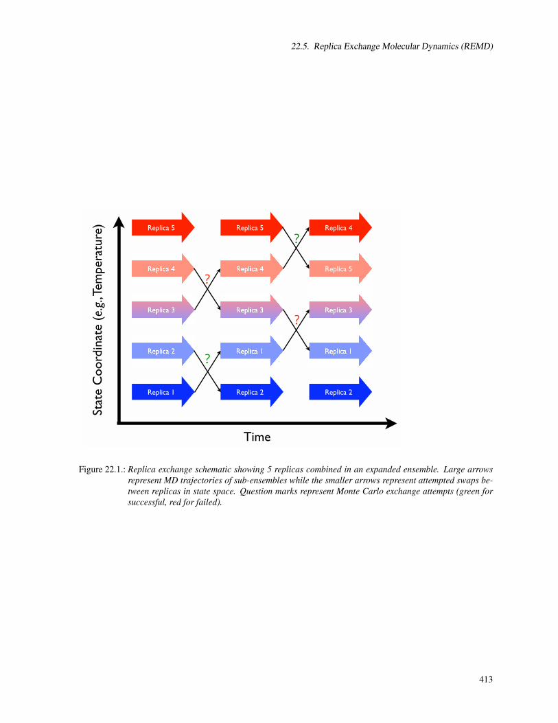
22.5. Replica Exchange Molecular Dynamics (REMD)
Stat
e C
oord
inat
e (e.g., T
emper
ature
)
Time
Replica 1
Replica 2
Replica 4
Replica 5
Replica 2
Replica 1
Replica 4
Replica 5
Replica 2
Replica 1
Replica 5
Replica 4
?
?
?
?
Figure 22.1.: Replica exchange schematic showing 5 replicas combined in an expanded ensemble. Large arrowsrepresent MD trajectories of sub-ensembles while the smaller arrows represent attempted swaps be-tween replicas in state space. Question marks represent Monte Carlo exchange attempts (green forsuccessful, red for failed).
413

22. Free energies
22.5.2. Running REMD simulations
In order to run REMD simulations, sander and pmemd use the multisander (and multipmemd) machinery thatallows multiple MD trajectories to be run in the same simulation. This mode of sander and pmemd is used slightlydifferently than their normal operation, and is described in Section 18.11.
There are two new variables that must be present in the &cntrl section of the mdin files of each replica for allREMD simulations.
numexchg This is the number of exchange attempts that will be performed between replica pairs
nstlim This is the number of MD steps that will be performed between exchange attempts
There are also additional command-line flags that should be placed on the command-line (with the groupfile),described below:1
-rem <#> This flag defines the type of replica exchange that will be run for 1-D REMD. The allowed values are 1(T-REMD), 3 (H-REMD), and 4 (pH-REMD). Each approach is described in later sections.
-remlog <remlog_file> This flag specifies the name of the log file that contains information about each of thereplicas during each exchange attempt. The default value is rem.log.
-remtype <remtype_file> This flag specifies a filename for the remtype file; this file provides helpful informationabout the current replica run. For reservoir REMD runs it also prints reservoir information. Default isrem.type
Some specialized types of REMD simulations have additional command-line flags that will be described in futuresections.
Note the change in the meaning of nstlim. For standard MD, nstlim is the total number of MD steps that willbe performed. For REMD, simulations, on the other hand, nstlim is the number of steps between replica exchangeattempts and the total number of steps is equal to nstlim×numexchg. The nstlim variable, then, is related to theinverse of the exchange attempt frequency (EAF) in REMD simulations. The value of numexchg must be the samefor each input file, or the program will hang indefinitely as those replicas assigned more exchange attempts wait toexchange data with replicas that have already finished. We also strongly suggest keeping nstlim the same as wellto avoid making replicas with fewer steps wait for those with more steps to finish.
Currently, Amber only supports running replica exchange simulations at constant volume for explicit solventsimulations, and all replicas must have the same volume. Therefore, the equilibration stage of each replica shouldbegin after the original system was run at constant pressure to stabilize the density (and volume).
Amber currently supports 4 types of exchange attempts: Temperature REMD (T-REMD), Hamiltonian REMD(H-REMD), constant pH REMD (pH-REMD), and replica exchange self-guided Langevin dynamics (RXSGLD).Multi-dimensional REMD simulations (defined by 2 or more state parameters) are also supported. The instructionsgiven above apply to all REMD simulations, but instructions for running REMD simulations in general stronglydepend on the type of exchange being attempted. Additional details for running REMD simulations are providedin the following sections for each type of exchange attempt.
22.5.3. Running Temperature REMD simulations
In temperature REMD (T-REMD), replicas are distinguished based on the temperature of their temperature bath.In general, each replica should differ from each other only by their target temperature, temp0, specified in the mdinfile for each replica. The N replicas are first sorted in an array by their target temperatures, so the ordering of thereplicas in the groupfile is irrelevant. Neighboring residues attempt to exchange every nstlim MD steps, withthe exchange partners alternating each replica exchange attempt. For example, if replicas 2 and 3 attempt to swapthe first time then replicas 1 and 2 will attempt to swap the next time (as will replicas 3 and 4). Topologically,the N temperature-sorted replicas form a loop, in which the first and the last replicas are neighbors. Therefore,N/2 exchanges are attempted every nstlim steps. The exchange success rate is computed via a Metropolis Monte
1Some specialized types of REMD simulations have additional command-line flags that will be described in the later sections.
414

22.5. Replica Exchange Molecular Dynamics (REMD)
Carlo move shown in Eq. 22.10 that satisfies detailed balance for swapping temperatures. If the exchange isallowed between the pair, the temperature between the replicas is swapped before MD resumes. The velocities ofeach replica involved in successful exchange are then adjusted by the scaling factor
√Tnew/Told where Told is the
temperature before the exchange and Tnew is the temperature after. This velocity scaling is done to ensure that eachstructure is immediately adjusted to its new target temperature. After the exchange calculation, the MD resumesfor nstlim steps until the next exchange attempt (in which the exchange partners alternated with respect to theprevious exchange attempt).
Pi, j = min
1,exp [−(βi−β j)(E j−Ei)]
(22.10)
Before starting a replica exchange simulation, an optimal set of temperatures should be determined so that theexchange ratio is roughly a constant. This spacing of the replicas in temperature-space determines the probabilityof exchange among the replicas, and the user is referred to the literature for a more complete description of theinfluence of various factors on the exchange probability. A useful resource for generating a series of temperatureswith a specific exchange success probability can be found online at http://folding.bmc.uu.se/remd/.
Each replica requires (for input files) or generates (for output files) its own mdin, inpcrd, mdout, mdcrd, restrt,mdinfo, and associated files. The names are provided through the specification of a groupfile on the command linewith the -groupfile groupfile option. The groupfile file contains a separate command line for each of the replicas ormultisander instances, as described in Section 18.11. To choose the number of replicas or multisander instances,the -ng N command line option is used (in this case to specify N separate instances.)
For example, an 4-replica REMD job will need 4 mdin and 4 inpcrd files. Then, the groupfile might look likethis:
#
# multisander or replica exchange group file
#
-O -i mdin.rep1 -o mdout.rep1 -c inpcrd.rep1 -r restrt.rep1 -x mdcrd.rep1
-O -i mdin.rep2 -o mdout.rep2 -c inpcrd.rep2 -r restrt.rep2 -x mdcrd.rep2
-O -i mdin.rep3 -o mdout.rep3 -c inpcrd.rep3 -r restrt.rep3 -x mdcrd.rep3
-O -i mdin.rep4 -o mdout.rep4 -c inpcrd.rep4 -r restrt.rep4 -x mdcrd.rep4
Note that for T-REMD the mdin and inpcrd files are not required to be ordered by their target temperatures sincethey will not remain sorted during the simulation. Sorting is performed automatically at each REMD iteration asdescribed above. Thus one can restart REMD simulations without modifying the restart files from the previousREMD run (see below for more information about restarting REMD).
It is important when running T-REMD to ensure that each topology file is equivalent and the input files differ onlyin the temperature (temp0), and that all explicit solvent calculations are run at constant volume. Because Eq. 22.10was derived under the assumption that exchanging replicas only swapped temperatures, only the temperature canvary between replicas. Satisfying this requirement is left to the user, and no warnings or checks are implementedif this assumption is violated.
22.5.3.1. Restarting REMD simulations
It is recommended that each REMD run generate a new set of output files (such as mdcrd), but for convenienceone may use -A in the command line in order to append output to existing output files. This can be a useful optionwhen restarting REMD simulations. If -A is used, files that were present before starting the REMD simulation areappended to throughout the new simulation. If -O is used, any files present are overwritten. The recommendedinput file settings for restarting a REMD simulation are ig=-1 to use the wall clock for the pseudo-random numbergenerator seed, ntxo=2 to write a NetCDF restart file, ioutfm=1 to write NetCDF trajectories, irest=1 to restart, andntx=5 to read velocities; the first three should be used in the initial calculation.
At the end of a REMD simulation, the target temperature of each replica is most likely not the same as it wasat the start of the simulation (due to successful exchanges). If one wishes to continue this simulation, sander orpmemd will need to know how the target temperature has changed. Since the target value is normally specifiedin the mdin file (via temp0), the previous mdin files would all need to be modified to reflect changes in target
415

22. Free energies
temperature of each replica. In order to simplify this process, sander and pmemd write the final target temperatureas additional information in the restart files during a T-REMD simulation. When a T-REMD simulation is started,the program will check to see if the target temperature is present in the restart file. If it is present, this value willoverride the value in the mdin file. In this manner, one can restart the simulation from the set of restart files andsander or pmemd will automatically update the target temperature of each replica to correspond to the final valuefrom the previous run. If the target temperature is not present (as would be the case for the first REMD run), thecorrect values must be present in the mdin files.
22.5.3.2. Content of the output files
It is important to note that in the current implementation of T-REMD all output is by replica only, not bytemperature! To facilitate post processing of trajectory data by temperature, the temperature must be specified foreach snapshot. For NetCDF trajectories, adding this information is simple because NetCDF is an extensibleformat. We strongly recommend that you always use NetCDF trajectories, especially for REMD simulations. ForASCII formatted trajectories, a header line is written to each frame just before the coordinates. This header linehas the format:
REMD <replica#> <exchange#> <step#> <Temperature>
PTRAJ and CPPTRAJ are be able to read trajectories with this new format.The rem.log file for T-REMD simulations has the following format:
# Replica Exchange log file
# numexchg is 5
# REMD filenames:
# remlog= rem.log
# remtype= rem.type
# Rep#, Velocity Scaling, T, Eptot, Temp0, NewTemp0, Success rate (i,i+1), ResStruct#
# exchange 1
1 1.15 0.00 -10.46 300.00 400.00 0.00 -1
2 1.04 0.00 -10.46 325.00 350.00 2.00 -1
3 0.96 0.00 -10.46 350.00 325.00 0.00 -1
4 0.87 0.00 -10.46 400.00 300.00 2.00 -1
# exchange 2
1 0.94 312.03 -6.81 400.00 350.00 1.00 -1
2 1.07 280.77 -3.95 350.00 400.00 1.00 -1
3 -1.00 247.11 -10.58 325.00 325.00 1.00 -1
4 -1.00 271.12 -14.15 300.00 300.00 0.00 -1
# exchange 3
1 0.96 305.31 -11.02 350.00 325.00 0.67 -1
2 0.87 288.89 -12.45 400.00 300.00 1.33 -1
3 1.04 290.99 -13.30 325.00 350.00 1.33 -1
4 1.15 256.19 -12.83 300.00 400.00 0.00 -1
The columns, listed in order, are the replica number, velocity scaling factor, the instantaneous temperature, thepotential energy of the structure, the target temperature before the exchange attempt, the target temperature afterthe exchange attempt, the average success rate, and the reservoir structure number. The replica number neverchanges since replicas swap target temperatures. When the velocity scaling factor is -1, the exchange attemptfailed and velocities are not altered. For successful exchange attempts, velocites are either scaled up (when thenew target temperature is higher than the old one) or down (when the new target temperature is lower than the oldone). Success rates are calculated as #successes/# tries× 2, where the factor of 2 is used because each pair ofneighboring replicas attempts to exchange every other exchange attempt. In the beginning of the log file, this maylead to unusual success rates, but after a large number of exchange attempts the values will normalize. Successrates are computed as the exchange success rate between the original temperature (Temp0 column) and the nexthighest temperature in the temperature ladder (not necessarily the temperature it just attempted to exchange with).The success rate for the highest temperature is often 0 since it reflects the success rate between the highest andlowest temperatures.
416
22.5. Replica Exchange Molecular Dynamics (REMD)
All temperatures are reported in Kelvin and all energies in kcal/mol.
22.5.3.3. Cautions when using replica exchange
While many variations of replica exchange have been tested with sander, all possible variations have not beentested and the option is intended for use by advanced researchers that already have a comprehensive understandingof standard molecular dynamics simulations. Caution should be used when creating REMD input files. Amberwill check for the most obvious errors but due to the nature of the multiple output files the reason for the error maynot be readily apparent. The following is only a subset of things that users should keep in mind:
1. The number of replicas must be an even number (so that all replicas have a partner for exchange).
2. Temp0 values for each replica must be unique for Temperature-based REMD.
3. Other than temp0 mdin files should be identical.
4. Temp0 values should not be changed in the nmropt=1 weight change section.
5. A groupfile is required.
6. If high temperatures are used, it may be necessary to use a smaller time step and possibly restraints to preventcis/trans isomerization or chirality inversion.
7. Due to increased diffusion rates at high temperature, it may be good to use iwrap=1 to prevent coordinatesfrom becoming too large to fit in the restart format. An alternative to this is, of course, to use the defaultNetCDF restart files (ntxo=2).
8. Note that the optimal temperature range and spacing will depend on the system. The user is strongly recom-mended to read the literature in this area.
9. Constant pressure is not supported for REMD simulations. This means NTP must be 0.
22.5.3.4. Replica exchange example
Below is an example of an 8-replica REMD run on 16 processors, (note that launching a MPI program variesfrom computer to computer).
mpirun -np 16 sander.MPI -ng 8 -groupfile groupfile -rem 1
Here is the groupfile:
#
# multisander or replica exchange group file
#
-O -i mdin.rep1 -o mdout.rep1 -c inpcrd.rep1 -r restrt.rep1 -x mdcrd.rep1
-O -i mdin.rep2 -o mdout.rep2 -c inpcrd.rep2 -r restrt.rep2 -x mdcrd.rep2
-O -i mdin.rep3 -o mdout.rep3 -c inpcrd.rep3 -r restrt.rep3 -x mdcrd.rep3
-O -i mdin.rep4 -o mdout.rep4 -c inpcrd.rep4 -r restrt.rep4 -x mdcrd.rep4
-O -i mdin.rep5 -o mdout.rep5 -c inpcrd.rep5 -r restrt.rep5 -x mdcrd.rep5
-O -i mdin.rep6 -o mdout.rep6 -c inpcrd.rep6 -r restrt.rep6 -x mdcrd.rep6
-O -i mdin.rep7 -o mdout.rep7 -c inpcrd.rep7 -r restrt.rep7 -x mdcrd.rep7
-O -i mdin.rep8 -o mdout.rep8 -c inpcrd.rep8 -r restrt.rep8 -x mdcrd.rep8
This input specifies that T-REMD should be used (-rem 1), with 8 replicas (-ng 8) and 2 processors per replica (-np16). Note that the total number of processors should always be a multiple of the number of replicas.
417
22. Free energies
22.5.3.5. Replica exchange using a hybrid solvent model
This section describes an advanced feature of Amber.[142, 143] Users that are not already comfortable with stan-dard replica exchange simulations should likely get more experience with them before attempting hybrid solventREMD calculations.
For large systems, REMD becomes intractable since the number of replicas needed to span a given temperaturerange increases roughly with the square root of the number of degrees of freedom in the system. Recognizing thatthe main difficulty in applying REMD with explicit solvent lies in the number of simulations required, rather thanjust the complexity of each simulation, we recently developed a new approach in which each replica is simulatedin explicit solvent using standard methods such as periodic boundary conditions and inclusion of long-range elec-trostatic interactions using PME. However, the calculation of exchange probabilities (which determines the tem-perature spacing and thus the number of replicas) is handled differently. Only a subset of closest water moleculesis retained, with the remainder temporarily replaced by a continuum representation. The energy is calculated usingthe hybrid model, and the exchange probability is determined. The original solvent coordinates are then restoredand the simulation proceeds as a continuous trajectory with fully explicit solvation. This way the perceived systemsize for evaluation of exchange probability is dramatically reduced and fewer replicas are needed.
An important difference from existing hybrid solvent models is that the system is fully solvated throughoutthe entire MD simulation, and thus the distribution functions and solvent properties should not be affected by theuse of the hybrid model in the exchange calculation. In addition, no restraints of any type are needed for thesolvent, and the solute shape and volume may change since the solvation shells are generated for each replicaon the fly at every exchange calculation. Nearly no computational overhead is involved since the calculationis performed infrequently as compared to the normal force evaluations. Thus the hybrid REMD approach canemploy more accurate continuum models that are too computationally demanding for use in each time step of astandard molecular dynamics simulation. However, since the Hamiltonian used for the exchange differs from thatemployed during dynamics, these simulations are approximate and are not guaranteed to provide correct canonicalensembles.
At each exchange calculation sander will create the hybrid system based on the current coordinates for the fullysolvated system. This is done by calculating the distance of each water oxygen to the nearest solute atom, andsorting the water by increasing shortest distance. The closest numwatkeep are retained and the potential energyis calculated using the GB model specified by hybridgb. After the energy calculation the fully solvated system isrestored.
For a more complete example, users are directed to the hybridREMD test case (in the rem_hybrid subdirectory)in the Amber test directory.
numwatkeep The number of explicit waters that should be retained for the calculation of potential energy to beused for the exchange calculation. Before each exchange attempt, the closest numwatkeep waters willbe retained (closest to the solute) and the rest will be temporarily removed and then replaced after theexchange probability has been calculated. The default value is -1, indicating that all waters shouldbe retained (standard REMD). A value of 0 would direct Amber to remove all of the explicit water(as in MM-PBSA) while a nonzero value will result in some water close to the solute being retainedwhile the rest is removed. Currently it is not possible to select a subset of solute atoms for determiningwhich waters are "close". Determining the optimal numwatkeep value is a topic of current research.
hybridgb Specifies which GB model should be used for calculating the PE of the stripped coordinates, equivalentto the igb variable. Currently only hybridgb values of 1, 2, and 5 are supported.
Cautions: Hybrid-REMD has not been extensively tested. The following would not be expected to work withoutfurther modification of the code:
1. Only the water is imaged for the creation of the stripped system. Care should be taken with dimers (such asDNA duplexes) to ensure that the imaging is correct.
2. Explicit counterions should probably not be used.
3. The choice of implicit solvent model will likely have a large effect on the resulting ensemble.
418

22.5. Replica Exchange Molecular Dynamics (REMD)
22.5.3.6. Reservoir REMD
The ability to perform REMD with a structure reservoir [423, 424] has been implemented in Amber as of version10. Although REMD can significantly increase the efficiency of conformational sampling, obtaining convergeddata can still be challenging. This is particularly true for larger systems, as the number of replicas needed to span agiven temperature range increases with the square root of the number of degrees of freedom in the system. Anotherconsideration is that the folding rate of a peptide tends not to be as dependent on temperature as the unfolding rate,making the search for native peptide structures in higher temperature replicas more problematic; in the case wherea native-like structure is found it will almost always be exchanged to a lower temperature replica, requiring a repeatof the search process. In addition, the exchange criterion in REMD assumes a Boltzmann-weighted ensemble ofstructures, which is typically not the case at the start of a REMD simulation. Although the exchange criterionwill eventually drive each replica toward a Boltzmann-weighted ensemble of structures, this essentially means thatuntil all of the replicas are converged, none of the replicas are converged.
Reservoir REMD is a method which can significantly enhance the rate of convergence and reduce the highcomputational expense of standard REMD simulations. An ensemble of structures (or reservoir) is generatedat high temperature, then linked to lower temperatures via REMD. Periodic exchanges are attempted betweenrandomly chosen structures in the reservoir and the highest temperature replica. If the structure reservoir is alreadyBoltzmann-weighted,[423] convergence is significantly enhanced as the lower temperature replicas simply act tore-weight the reservoir ensemble - in essence all of the searching has been accomplished from the start. This isin contrast to standard REMD where all the replicas are run simultaneously, and the computational expense forrunning long simulations must be paid for each of the replicas even though only a few high-temperature ones maybe contributing to sampling of new basins.
One major advantage of this approach is that a converged ensemble of conformations needs to be generatedonly once and only for one temperature. Typically this temperature should be high enough to facilitate crossingof energy barriers, but low enough that there is still a measureable fraction of native structure present. Anotheradvantage is that exchanges with the reservoir do not need to be time-correlated with the replica simulations;folding events sampled during reservoir generation can provide multiple native structures for the other replicas.
It may not always be possible however to generate a Boltzmann-weighted ensemble of structures (e.g. for alarge molecule in explicit solvent). In such cases it is possible to use a non-Boltzmann weighted reservoir bymodifying only the exchange criterion between the reservoir and the highest temperature replica. If the weight ofall structures in the reservoir is set to 1, this corresponds to a completely flat distribution across the free energylandscape. Alternatively, weights can be assigned to structures based on various structural properties. In the currentimplementation, weights are assigned to structures via dihedral bin clustering, wherein clusters are identified byunique configurations of user-defined dihedral angles.
There are several new command line arguments that pertain to Reservoir REMD:
-rremd Type of reservoir to use.
= 0 No reservoir (Default)
= 1 Boltzmann-weighted reservoir
= 2 Non-Boltzmann weighted reservoir where the weight of each structure in the reservoir is assumed to be1/N
= 3 Non-Boltzmann weighted reservoir with weights defined by dihedral angle binning.
-reservoir Specifies the file name prefix for reservoir structures. Reservoir structure files should be in the restartfile format MDRESTRT, and are expected to be named according to the format <name>.XXXXXX, whereXXXXXX is a 6 digit integer, e.g. frame.000001. Default is "reserv/frame". IMPORTANT NOTE: Struc-ture numbering should begin at 1.
-saveene specifies the file containing energies of the structures in the reservoir (default filename is "saveene").This file must contain a header line with format:
<# reservoir structures> <reservoir T> <#atoms> <random seed><velocity flag>
419
22. Free energies
If the velocity flag =1 then velocity information will be read from the reservoir structure files, otherwise(if velocity flag =0) velocities will be assigned to the structure based on the reservoir temperature. Afterthe header line there should be a line containing the potential energy of each reservoir structure. IMPOR-TANT NOTE: For reservoir REMD with dihedral bin clustering (rremd==3) each potential energy shouldbe followed by the cluster # that reservoir structure belongs to.
-clusterinfo For reservoir REMD with dihedral bin clustering (rremd==3) this file specifies what dihedrals areused and the binsize, as well as what cluster each reservoir structure belongs to. Default is "cluster.info".File has the following format:
<# Dihedral Angles><atom# 1> <atom# 2> <atom# 3> <atom# 4> [Dihedral 1]
. .
. .
. .
<atom# 1> <atom# 2> <atom# 3> <atom# 4> [# Dihedral Angles]
<Total # Clusters><Cluster #> <Weight><Bin1><Bin2>...<Bin #Dihedral Angles> [Cluster 1]
. .
. .
. .
<Cluster #> <Weight><Bin1><Bin2>...<Bin #Dihedral Angles> [# Clusters]
The first line is the number of dihedral angles that will be binned, following the definition of those dihedralangles (4 atoms using sander atom #s, starting from 1) and the bin size for each dihedral angle. Next is thetotal # of clusters followed by lines providing information about each cluster: the cluster number, weightand ID as defined by dihedral binning. The ID is composed of consecutive 3 digit integers, 1 for eachdihedral angle. For example, a structure belonging to cluster 7 with a weight of 2 with 2 dihedral anglesthat fall in bins 3 and 8 would look like:
7 2 003008
22.5.4. Hamiltonian replica exchange
Instead of spacing replicas throughout temperature space, you can also space replicas throughout “Hamiltonianspace.” That is, every replica has a different Hamiltonian, or energy function, and exchange attempts occur betweenadjacent Hamiltonians. With sander and pmemd, Hamiltonian replica exchange is implemented by exchangingcoordinates between replicas and evaluating the energy of that new structure. The corresponding detailed balanceequation that is used to compute the exchange probability is shown in Eq. 22.11. This option is enabled by using-rem 3 on the command-lines in the groupfile.
Pi→ j = min1,exp(−β1 [H1(x2)−H1(x1)]−β2 [H2(x1)−H2(x2)]) (22.11)
Here, state i refers to the replica combination [β1H1(x1), β2H2(x2)] and state j refers to the replica combination[β1H1(x2), β2H2(x1)]. Eq. 22.11 assumes that only coordinates are traded between exchanging replicas, but allowsfor the temperatures to differ. The temperature does not exchange upon a successful attempt, but velocities areswapped following successful exchange attempts and scaled by
√Tnew/Told to match the target temperature of
their new replica.
22.5.4.1. Free Energy Perturbation
Upon closer inspection of Eq. 22.11, we can see a close resemblance to Free Energy Perturbation[420, 425]
∆Ga→b =−kBT ln [exp(−β (Eb−Ea))] (22.12)
420

22.5. Replica Exchange Molecular Dynamics (REMD)
We can see that for every exchange attempt, the required ∆E is calculated in both directions. The value for thefree energy (in both directions) is accumulated and reported in the rem.log file each time an exchange is attempted.
For replica exchange free energy perturbation (REFEP), multiple topology files are often needed that correspondto a value of an alchemical parameter, λ , similar to thermodynamic integration. The ParmEd program includedwith AmberTools can be used to generate the intermediate topology files by scaling charges and/or van der Waalsparameters. In this case, because coordinates are exchanged, each replica tracks a particular Hamiltonian and setof control variables, rather than a sequence of configuations. Note this is the opposite behavior of T-REMD inwhich replicas change temperatures but keep the same sequence of configurations.
22.5.4.2. Umbrella Sampling
Hamiltonian exchange can be used to perform replica exchange umbrella sampling [426] using the NMR flatwell restraints. In this case, every line of the group file needs a different restraint file in which the center ofthe biasing umbrella changes. Each replica tracks a particular umbrella location rather than a replica trajectory.Note this is the opposite behavior of T-REMD in which replicas change temperatures but keeps the same replicatrajectory.
22.5.4.3. Steps for running H-REMD simulations
Note: before running Hamiltonian replica exchange (H-REMD), you should be familiar with Temperaturereplica exchange (T-REMD) simulations. H-REMD simulations are set up similarly to T-REMD simulations. Eachreplica is specified on a line of a groupfile and is run with multisander. Each replica differs either by simulationcontrol parameters in the input file (e.g., for umbrella sampling replica exchange[426] or REXAMD [427, 428]) orparameters in the topology file (e.g., REFEP).
• The majority of H-REMD settings are similar to T-REMD. A groupfile is needed. The number of replicasmust be an even number (so that all replicas have a partner for exchange). Constant pressure is not supportedfor REMD simulations. This means ntp must be 0.
• Depending on the type of H-REMD, all replicas may have different force fields/control variables (if thedifferences are too large, the exchange probability may suffer)
• The order of the replicas in the groupfile is very important. As a general rule in all H-REMD simulations, theleast different Hamiltonians (replicas) should be neighbors. Because this method is relatively new, there arevery limited discussions in the literature about the optimum positions of replicas in the Hamiltonian ladder[429, 430]. Exchange neighbors are defined by adjacent lines in the groupfile (i.e., each replica exchanges‘right’ or ‘up’ with the replica defined by the line above and exchanges ‘left’ or ‘down’ with the replicadefined by the line below in the groupfile).
• For editing the prmtop, e.g., in the case of REFEP, there is a python script in AmberTools, parmed, whichfacilitates the modifications of Amber topology files. See Section 14.2 for details.
• In H-REMD, each replica has a different Hamiltonian. In contrast to T-REMD, neighbor replicas exchangetheir conformations, which means each replica keeps its initial Hamiltonian and there is no need for post-processing (i.e., using ptraj or cpptraj) to extract sub-ensembles. However, you will have to post-process inorder to reconstruct replica-based time series.
To enable H-REMD the -rem flag on the command-line must be given the value 3. H-REMD simulations requirethe same input files as T-REMD simulations and generates the same output files. The output printed in the remlogfile differs significantly from that found in the remlog file for T-REMD, however. Example remlog output forH-REMD is shown below:
# Replica Exchange log file
# numexchg is 10000
# REMD filenames:
# remlog= remlog
# remtype= rem.type
421

22. Free energies
# Rep#, Neibr#, Temp0, PotE(x_1), PotE(x_2), left_fe, right_fe, Success, Success rate (i,i+1)
# exchange 1
1 8 300.00 -12783.23 -12755.40 -16.39 0.00 F 0.00
2 3 300.00 -12839.84 -12802.56 0.00 -0.05 T 2.00
3 2 300.00 -12802.60 -12839.79 -0.04 0.00 T 0.00
4 5 300.00 -12847.41 -12858.37 0.00 -0.78 F 0.00
5 4 300.00 -12858.19 -12846.63 0.18 0.00 F 0.00
6 7 300.00 -12859.65 -12833.42 0.00 0.30 T 2.00
7 6 300.00 -12833.63 -12859.95 -0.21 0.00 T 0.00
8 1 300.00 -12771.63 -12766.84 0.00 -16.23 F 0.00
# exchange 2
1 2 300.00 -12825.03 -13147.73 0.00 -0.62 F 0.00
2 1 300.00 -13148.20 -12824.42 -0.47 0.00 F 1.00
3 4 300.00 -13136.97 -12823.77 0.00 0.62 T 1.00
4 3 300.00 -12823.32 -13137.59 0.44 0.00 T 0.00
5 6 300.00 -12919.25 -13181.18 0.00 -0.41 T 1.00
6 5 300.00 -13180.48 -12918.84 0.70 0.00 T 1.00
7 8 300.00 -13162.39 -12775.37 0.00 0.16 T 1.00
8 7 300.00 -12775.59 -13162.55 -0.22 0.00 T 0.00
...
The columns, in order, are the replica number, the exchange partner for this attempt, the target temperature, thepotential energy of the current structure, the potential energy of the proposed structure, the free energy differencecalculated via Eq. 22.12 for all exchanges to the ‘left’ (or ‘up’ in the Hamiltonian ladder), all free energies forexchanges to the ‘right’ (or ‘down’ in the Hamiltonian ladder), whether the exchange attempt succeeded (T) or not(F), and the average success rate. For each step, the only free energy values printed are those between replicas thatattempted to exchange. All free energies between non-exchanging pairs are set to 0 for that step. Therefore, the‘final’ free energies can be found by summing the respective terms from the last two exchanges in the remlog file.All energies have units of kcal/mol, and temperatures have units of Kelvin.
22.5.4.4. An example
When running H-REMD, the format of the groupfile is very similar to that in T-REMD, but specific detailsdepend on the type of simulation being performed. In the case of REFEP, the groupfile may look like thefollowing:
-O -i mdin -p prmtop.0 -c inpcrd.0 -suffix 000
-O -i mdin -p prmtop.1 -c inpcrd.1 -suffix 001
-O -i mdin -p prmtop.2 -c inpcrd.2 -suffix 002
-O -i mdin -p prmtop.3 -c inpcrd.3 -suffix 003
-O -i mdin -p prmtop.4 -c inpcrd.4 -suffix 004
-O -i mdin -p prmtop.5 -c inpcrd.5 -suffix 005
-O -i mdin -p prmtop.6 -c inpcrd.6 -suffix 006
-O -i mdin -p prmtop.7 -c inpcrd.7 -suffix 007
Notice how the topology file differs in each case, but the input file remains the same. An example groupfile forumbrella sampling may look like the following:
-O -i mdin.0 -p prmtop -c inpcrd.0 -suffix 000
-O -i mdin.1 -p prmtop -c inpcrd.1 -suffix 001
-O -i mdin.2 -p prmtop -c inpcrd.2 -suffix 002
-O -i mdin.3 -p prmtop -c inpcrd.3 -suffix 003
-O -i mdin.4 -p prmtop -c inpcrd.4 -suffix 004
-O -i mdin.5 -p prmtop -c inpcrd.5 -suffix 005
-O -i mdin.6 -p prmtop -c inpcrd.6 -suffix 006
-O -i mdin.7 -p prmtop -c inpcrd.7 -suffix 007
Notice in this case how the topology file is the same but the input file differs in each case (which is where thecenter of the umbrella is defined). Like T-REMD, sander.MPI (or pmemd.MPI) are executed via the followingcommand:
422

22.5. Replica Exchange Molecular Dynamics (REMD)
mpirun -np 16 sander.MPI -ng 8 -groupfile groupfile -rem 3
Note that the particular method for launching an MPI program may depend on your MPI implementation. Also,pmemd requires at least 2 threads per replica, whereas sander will work with just 1.
22.5.5. RXSGLD: Replica exchange using Self-Guided Langevin Dynamics
RXSGLD utilizes the guiding force, sgft or tempsg, to define replicas. SGLD simulations are performed forreplicas[375]. Please refer to Section 21.1 about how to set up SGLD simulations. When temperature is the samefor all replicas, the replica exchange ratios are high and so is the conformational search efficiency. RXSGLD is analternative to SGLD, SGLDfp, or SGLDg to achieve efficient conformational search while being able to obtain thecanonical ensemble distribution. RXSGLD is turned on if isgld is set to 1 or 3 in the sander or pmemd input filewhen performing replica exchange simulations (i.e., rem > 0).
For the convenience of reference, we define replicas as non-interacting identical simulation systems and definestages as simulation conditions between which replicas transit. In T-REMD, stages are different by temperatures,while in RXSGLD, stages are different by the strength of guiding forces, as defined by sgld or tempsg. Forexample, we can set tempsg=300, 310, 325, 345, 370, 400, 440, and 500K for stages 1 to 8, respectively, whiletemp0=300K for all stages. In RXSGLD, temperatures in different stages can be the same or different from eachother; however, it is prefered to keep all temperatures the same to achieve high replica exchange efficiency.
Because the temperatures of different stages may be the same, the stages are given a ID from 1 to Nrep. LikeT-REMD, each RXSGLD trajectory file is for each replica. Unlike T-REMD, the frames of RXSGLD trajectoriesare proceeded by the following information:
RXSGLD <replica#> <exchange#> <step#> <stage ID>
The output from RXSGLD contains the following lines:
TEMP0= <temp0> SGFT= <sgft> TEMPSG= <tempsg> STAGE= <stag ID> REPNUM= <rep#> EXCHANGE= <exchange#>
RXSGLD trajectories can be processed with PTRAJ analogously to T-REMD trajectories: merely replacetemperatures with stage IDs. For example, to extract the trajectory on stage 1, we can use the followingcommand:
ptraj rxsgld.top <<EOF
trajin rxsgld.trj.000 rxsgldtraj rxsgldid 1
trajout rxsgld.trj.stag 1
EOF
22.5.6. pH-REMD
In constant pH REMD, replicas attempt to exchange their solution pH values in much the same way as tem-peratures are exchanged in T-REMD. The idea of swapping pH in the discrete protonation state implementation(described in Section 23) was proposed by [Itoh et al. 421] and later implemented and evaluated in Amber. [422]The implementation here works very similarly to T-REMD, except each replica is given a different value of solvphin the mdin file instead of temp0. The exchange probability, shown in Eq. 22.13, is derived under the assumptionthat all replicas have the same temperature.
Pi→ j = min
1,exp[ln10
(NH+
i −NH+
j
)(pHi− pH j)
](22.13)
Where NH+
i is the number of titratable protons currently ‘active’ in state i.Before running pH-REMD simulations, you should first be familiar with running constant pH MD described in
Section 23, since it will help you set up each replica. Aside from the changes required to run at constant pH, settingup pH-REMD simulations is quite similar to setting up T-REMD simulations. Each replica should have the sametopology file, and all mdin files should be identical except for the value of solvph. Furthermore, each residueshould be titrating the same residues (this is very important). For instance, you cannot turn ‘off’ carboxylatetitrations at basic pH if your pH-REMD spans both acidic and basic conditions.
423

22. Free energies
22.5.6.1. Analyzing Output
The output from pH-REMD simulations is analyzed in the same way as standard constant pH simulations, withsome preprocessing required. Because the pH of each replica changes upon successful replica exchange attempts,each replica contains members from ensembles at all pHs. Therefore, you must use ptraj or cpptraj to extractensembles at each pH. To simplify the coding required, the pH is stored as the ‘temperature’ in each trajectory, sothe T-REMD machinery should be used in ptraj/cpptraj to extract desired ensembles.
The cpout files have additional information added to them to indicate which protonation states belong to whichensembles. This is done by printing the pH next to each record, as shown below.
Solvent pH: 3.00000
Monte Carlo step size: 5
Time step: 5
Time: 10.008
Residue 0 State: 3 pH: 3.000
Residue 0 State: 3 pH: 3.000
Residue 0 State: 3 pH: 3.500
Residue 0 State: 3 pH: 3.500
Residue 0 State: 3 pH: 2.000
Residue 0 State: 3 pH: 2.000
Residue 0 State: 3 pH: 2.500
You can see that the pH is changing between snapshots. In addition to generating pH-based trajectories, you alsomust generate pH-based cpout information that is stored in each cpout file. The replica pH is identified on eachline of the cpout file to aid in constructing the pH-specific protonation state ensembles. To aid with this, thecphstats program, described in Subsection 23.7.5, has an option to provide a “prefix” that defines the new filenames for the pH-specific cpout files that it builds from a list of each cpout file from a single pH-REMDsimulation. For example:
cphstats --fix-remd 1AKI.cpout 1AKI.cpout.000 1AKI.cpout.001 \
1AKI.cpout.002 1AKI.cpout.003
Assuming you ran replicas at pH 2, 3, 4, and 5, this will generate files 1AKI.cpout.pH_2.00, 1AKI.cpout.pH_3.00,1AKI.cpout.pH_4.00, and 1AKI.cpout.pH_5.00, with their respective ensembles. If you ran, for instance, 20 nsof simulation in chunks of 5 ns (so you ran 4 “chunks” after 3 restarts), you will need to run this command 4times—once for each simulation segment. You should analyze the resulting protonation state distribution usingthese newly-generated cpout files.
22.5.6.2. A pH-REMD Example
Below is an example in which 4 replicas are run at pH values of 2.0, 2.5, 3.0, and 3.5. The command belowshows an example of running this simulation on 8 processors (2 processors for each replica). Note that runningMPI programs may vary from computer to computer.
mpirun -np 8 sander.MPI -ng 4 -groupfile groupfile -rem 4 -remlog rem.log
The groupfile in this example is shown below:
-O -i phremd.pH2.0.mdin -cpin cpin -p ASPREF.top -c ASPREF.rst7
-O -i phremd.pH2.5.mdin -cpin cpin -p ASPREF.top -c ASPREF.rst7
-O -i phremd.pH3.0.mdin -cpin cpin -p ASPREF.top -c ASPREF.rst7
-O -i phremd.pH3.5.mdin -cpin cpin -p ASPREF.top -c ASPREF.rst7
424

22.5. Replica Exchange Molecular Dynamics (REMD)
The suffixes “.000”, “.001”, “.002”, and “.003” will be added to the output files from each of the replicas in orderto distinguish them from each other by default. This suffix can be changed using the “-suffix” flag for that replica.Any suffix provided this way will be applied to ALL output files, regardless of whether or not they are specified.This is only true for multi-sander and multi-pmemd simulations.
The resulting rem.log file looks like the following:
# Replica Exchange log file
# numexchg is 50
# REMD filenames:
# remlog= rem.log
# remtype= rem.type
# Rep#, N_prot, old_pH, new_pH, Success rate (i,i+1)
# exchange 1
1 1 2.000 3.500 0.0000
2 1 2.500 3.000 2.0000
3 1 3.000 2.500 0.0000
4 1 3.500 2.000 2.0000
# exchange 2
1 1 3.500 3.000 1.0000
2 1 3.000 3.500 1.0000
3 1 2.500 2.000 1.0000
4 1 2.000 2.500 1.0000
# exchange 3
1 1 3.000 2.500 0.6667
2 1 3.500 2.000 1.3333
3 1 2.000 3.500 0.6667
4 1 2.500 3.000 1.3333
# exchange 4
1 1 2.500 2.000 1.0000
2 1 2.000 2.500 1.0000
3 1 3.500 3.000 1.0000
4 1 3.000 3.500 1.0000
The columns are the current replica number (which never changes because pH is swapped between replicas), thetotal number of protons “active” on all of the titratable sites, the original solution pH, the new solution pH afterexchange, and the success ratio (multiplied by 2 to account for swapping neighbors each exchange attempt).
22.5.7. Multi-dimensional Replica Exchange
Multi-dimensional replica exchange refers to an expanded ensemble technique in which each subensemble (i.e.,each replica) is defined by multiple state parameters such as the temperature of the heat bath or the Hamiltonian.For such systems, an exchange attempt between two arbitrary replicas yields a complex equation for the exchangeprobability that must be derived and specified for each type of multi-dimensional exchange scheme. However,if exchange attempts between replica pairs are restricted to pairs that only differ in one state parameter, such asthe temperature, then the exchange probability equation reduces to the one used for that particular type of replicaexchange. Such an approach allows the existing exchange routines to be used in complex, multi-dimensionalreplica exchange simulations.
To implement the scheme described above, the entire expanded ensemble is subdivided into dimensions whichare further divided into groups. Each dimension is defined by a particular type of exchange attempt—namelytemperature exchange, Hamiltonian exchange, or pH exchange—and assigns every replica in the simulation to aparticular group. Each group is like a one-dimensional REMD simulation by itself—replicas differ only by the onethermodynamic state parameter used to define that particular dimension. Exchange attempts occur only betweennearest neighbors of a single replica group.
425
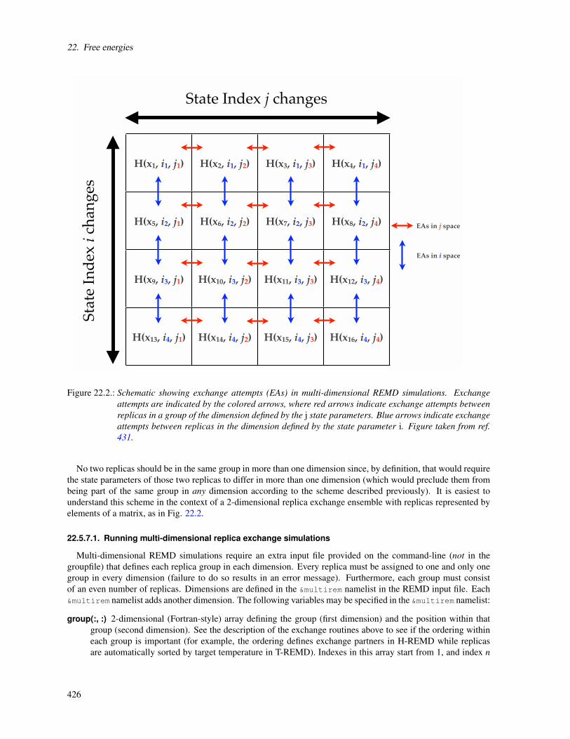
22. Free energies
H(x1, i1, j1) H(x2, i1, j2) H(x3, i1, j3) H(x4, i1, j4)
H(x5, i2, j1) H(x6, i2, j2) H(x7, i2, j3) H(x8, i2, j4)
H(x9, i3, j1) H(x10, i3, j2) H(x11, i3, j3) H(x12, i3, j4)
H(x13, i4, j1) H(x14, i4, j2) H(x15, i4, j3) H(x16, i4, j4)
Stat
e In
dex
i c
han
ges
State Index j changes
EAs in j space
EAs in i space
Figure 22.2.: Schematic showing exchange attempts (EAs) in multi-dimensional REMD simulations. Exchangeattempts are indicated by the colored arrows, where red arrows indicate exchange attempts betweenreplicas in a group of the dimension defined by the j state parameters. Blue arrows indicate exchangeattempts between replicas in the dimension defined by the state parameter i. Figure taken from ref.431.
No two replicas should be in the same group in more than one dimension since, by definition, that would requirethe state parameters of those two replicas to differ in more than one dimension (which would preclude them frombeing part of the same group in any dimension according to the scheme described previously). It is easiest tounderstand this scheme in the context of a 2-dimensional replica exchange ensemble with replicas represented byelements of a matrix, as in Fig. 22.2.
22.5.7.1. Running multi-dimensional replica exchange simulations
Multi-dimensional REMD simulations require an extra input file provided on the command-line (not in thegroupfile) that defines each replica group in each dimension. Every replica must be assigned to one and only onegroup in every dimension (failure to do so results in an error message). Furthermore, each group must consistof an even number of replicas. Dimensions are defined in the &multirem namelist in the REMD input file. Each&multirem namelist adds another dimension. The following variables may be specified in the &multirem namelist:
group(:, :) 2-dimensional (Fortran-style) array defining the group (first dimension) and the position within thatgroup (second dimension). See the description of the exchange routines above to see if the ordering withineach group is important (for example, the ordering defines exchange partners in H-REMD while replicasare automatically sorted by target temperature in T-REMD). Indexes in this array start from 1, and index n
426

22.5. Replica Exchange Molecular Dynamics (REMD)
corresponds to the nth replica defined in the groupfile. The suggested syntax for assigning to this variable isshown in the example below.
exch_type Defines the type of exchange that will be performed. Supported values (case-insensitive) are “tem-perature” (or “temp”), “Hamiltonian” (or “HREMD”), and “pH.” pH-REMD is not currently compatiblewith T-REMD in another dimension. Also, H-REMD/pH-REMD simulations are not expected to work well.pH-compatible temperature and umbrella exchange are planned for the future.
desc Description that will be printed in the rem.log files. This is for documentation purposes only, and will haveno effect on the simulation.
A sample input file that performs alchemical Hamiltonian-REMD in one dimension and Temperature-REMD inanother dimension is shown below.
Temperature REMD
&multirem
exch_type = ’TEMPERATURE’,
group(1,:) = 1,2,
group(2,:) = 3,4,
desc = ’Temperature exchange from 300K to 400K’
/
Hamiltonian REMD
&multirem
exch_type=’HAMILTONIAN’,
group(1,:) = 1,3,
group(2,:) = 2,4,
desc = ’Protonated ASP to Deprotonated ASP mutation’
/
Running multi-dimensional REMD simulations differs from running them in a single dimension. First, restartsand trajectories must be written in the NetCDF format (ntxo=2 for restarts and ioutfm=1 for trajectories). Thesechanges are applied by default for multi-dimensional REMD simulations. Next, the REMD input file is takenfollowing the -remd-file flag, and -rem should not be specified (it is set to -1 internally when -remd-file isread). An example command-line corresponding to the 4-replica example input file is shown below:
mpirun -np 4 sander.MPI -ng 4 -groupfile groupfile \
-remd-file remd.dim -remlog rem.log
The replica exchange information is stored in the remlog files written during the simulation. A separate remlog fileis written for each dimension with the name <prefix>.n where n is the nth dimension read from the REMD inputfile and <prefix> is the file name given on the command-line for the -remlog switch.
22.5.7.2. Restarting multi-dimensional replica exchange simulations
Some exchange types swap state parameters (e.g., temperature and pH) while others swap coordinates (Hamilto-nian), meaning that the ordering of the groupfile may change for restarts (see Fig. 22.3). To prevent requiring youto rewrite a new REMD file or groupfile each restart, the group number and replica position for each dimension isstored in the restart file. When irest=1 (see page 310) and the restart files contain the replica position information,the position of each replica in each dimension is set to the values stored in the restart file. This allows the samegroupfile and REMD file to be used for every subsequent restart. For general information on restarting a REMDsimulation seeSubsection 22.5.3.1.
Note, if the REMD index information is not present in the restart file or the REMD dimension information in therestart does not match what is defined in the REMD input file, the replica ordering will be assigned as it is definedin the REMD input file.
427
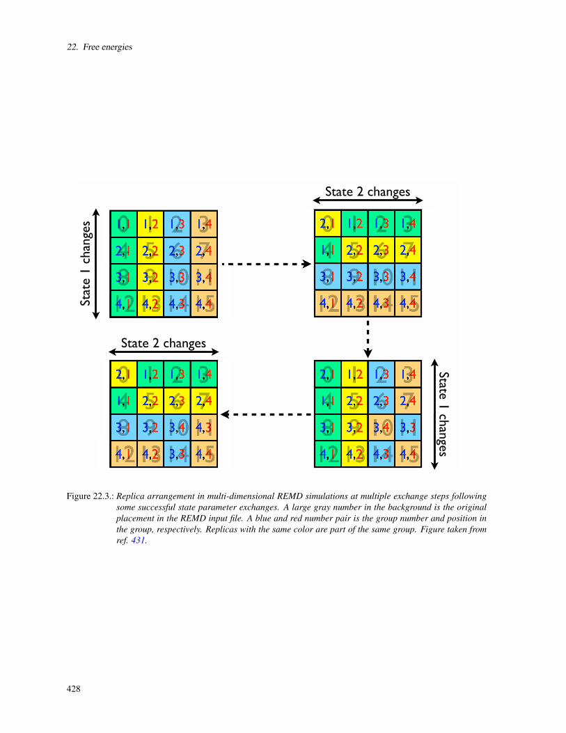
22. Free energies
1,1 1,2 1,3 1,4
2,1 2,2 2,3 2,4
3,1 3,2 3,3 3,4
4,1 4,2 4,3 4,4Stat
e 1 c
han
ges 2,1 1,2 1,3 1,4
1,1 2,2 2,3 2,4
3,1 3,2 3,3 3,4
4,1 4,2 4,3 4,4
State 2 changes
2,1 1,2 1,3 1,4
1,1 2,2 2,3 2,4
3,1 3,2 3,4 3,3
4,1 4,2 4,3 4,4
State 1 ch
anges
2,1 1,2 1,3 1,4
1,1 2,2 2,3 2,4
3,1 3,2 3,4 4,3
4,1 4,2 3,3 4,4
State 2 changes
Figure 22.3.: Replica arrangement in multi-dimensional REMD simulations at multiple exchange steps followingsome successful state parameter exchanges. A large gray number in the background is the originalplacement in the REMD input file. A blue and red number pair is the group number and position inthe group, respectively. Replicas with the same color are part of the same group. Figure taken fromref. 431.
428

22.6. Adaptively biased MD, steered MD, and umbrella sampling with REMD
22.5.7.3. Analyzing multi-dimensional replica exchange simulations
The REMD log file for each dimension is further divided into the log messages for each group, as shown below.
# Replica Exchange log file
# numexchg is 100
# Dimension 1 of 2
# Description: Temperature exchange from 300K to 400K
# exchange_type = TEMPERATURE
# REMD filenames:
# remlog= rem.log.1
# remd dimension file= remd.dim
# Rep#, Velocity Scaling, T, Eptot, Temp0, NewTemp0, Success rate (i,i+1), ResStruct#
# exchange 1 REMD group 1
1 -1.00 0.00 -40.69 300.00 300.00 0.00 0
2 -1.00 0.00 -19.77 400.00 400.00 0.00 0
# exchange 1 REMD group 2
1 -1.00 0.00 -66.78 300.00 300.00 0.00 0
2 -1.00 0.00 -46.06 400.00 400.00 0.00 0
# exchange 3 REMD group 1
1 -1.00 221.66 -34.00 300.00 300.00 0.00 0
2 -1.00 347.52 -29.09 400.00 400.00 0.00 0
# exchange 3 REMD group 2
1 -1.00 257.14 -63.10 300.00 300.00 0.00 0
2 -1.00 332.76 -26.73 400.00 400.00 0.00 0
The above example is shown for the first dimension (temperature) of the example REMD file shown in Sec.22.5.7.1. The columns are the same as those used in the corresponding 1-dimensional REMD simulation for thatexchange type.
To analyze structural properties, you must use cpptraj to properly snapshots into the appropriate replicas. SeeChapter 29 for more details.
22.6. Adaptively biased MD, steered MD, and umbrella sampling withREMD
22.6.1. Overview
The following describes a suite of modules useful for the calculation of the free energy associated with a reactioncoordinate σ(r1, . . . ,rN) (which is defined as a smooth function of the atomic positions r1, . . . ,rN):
f (ξ ) =−kBT ln⟨δ [ξ −σ(r1, . . . ,rN)]
⟩,
(the angular brackets denote an ensemble average, kB is the Boltzmann constant and T is the temperature) that isalso frequently referred to as the potential of mean force.
Specifically, new frameworks are provided for equilibrium umbrella sampling and steered molecular dynamicsthat enhance the functionality delivered by earlier implementations (described earlier in this manual), along witha new Adaptively Biased Molecular Dynamics (ABMD) method[432] that belongs to the general category of umbrellasampling methods with a time-dependent potential. Such methods were first introduced by Huber, Torda and vanGunsteren (the Local Elevation Method[433]) in the molecular dynamics (MD) context, and by Wang and Landau inthe context of Monte Carlo simulations[434]. More recent approaches include the adaptive force bias method[435],and the metadynamics method[436, 437]. All these methods estimate the free energy of a reaction coordinate froman evolving ensemble of realizations, and use that estimate to bias the system dynamics to flatten an effectivefree energy surface. Collectively, these methods may all be considered to be umbrella sampling methods with anevolving potential.
429

22. Free energies
The ABMD method grew out of attempts to speed up and streamline the metadynamics method for free energycalculations with a controllable accuracy. It is characterized by a favorable scaling in time, and only a few (two)control parameters. It is formulated in terms of the following equations:
mad2ra
dt2 = Fa +∂
∂raU[t|σ (r1, . . . ,rN)
],
∂U(t|ξ )∂ t
=kBTτF
G[ξ −σ (r1, . . . ,rN)
],
where the first ones represent Newton’s equations that govern ordinary MD (temperature and pressure regulationterms are not shown) augmented with an additional force coming from the time dependent biasing potential U(t|ξ )[U(t = 0|ξ ) = 0], whose time evolution is given by the second equation. G(ξ ) is a positive definite and symmetrickernel, which may be thought of as a smoothed Dirac delta function. For large enough τF (the flooding timescale)and small enough kernel width, the biasing potential U(t|ξ ) converges towards − f (ξ ) as t→ ∞.
Our numerical implementation of the ABMD method involves the use of a bi-weight kernel along with the use ofcubic B-splines (or products thereof) to discretize the biasing potential U(t|ξ ) w.r.t. ξ , and an Euler-like scheme fortime integration. ABMD admits two important extensions, which lead to a more uniform flattening of U(t|ξ )+ f (ξ )due to an improved sampling of the “evolving” canonical distribution. The first extension is identical in spirit tothe multiple walkers metadynamics [438, 439]. It amounts to carrying out several different MD simulations biasedby the same U(t|ξ ), which evolves via:
∂U(t|ξ )∂ t
=kBTτF
∑α
G[ξ −σ (rα
1 , . . . ,rαN)],
where α labels different MD trajectories. A second extension is to gather several different MD trajectories, eachbearing its own biasing potential and, if desired, its own distinct collective variable, into a generalized ensemblefor “replica exchange” with modified “exchange” rules[440–442]. Both extensions are advantageous and lead to amore uniform flattening of U(t|ξ )+ f (ξ ).
In order to assess and improve the accuracy of the free energies, the ABMDcmmmulations may need to be fol-lowed up with equilibrium umbrella sampling runs, which make use of the biasing potential U(t|ξ )cas is. Sucha procedure is very much in the spirit of adaptive umbrella sampling. With these runs, one calculates the biasedprobability density:
pB(ξ ) =⟨δ [ξ −σ(r1, . . . ,rN)]
⟩B.
The idea here is that if, as a result of an ABMD run, f (ξ )+U(t|ξ ) = 0 exactly, then the biased probability densitypB(ξ ) would be flat (constant). In practice, this is typically not the case, but one can use pB(ξ ) to “correct” thefree energy via:
f (ξ ) =−U(ξ )− kBT ln pB(ξ ).
This procedure has previously been successfully used to calculate accurate free energy maps for a number ofmolecules including several short peptides.
If you find any of these modules useful, we would ask you to kindly consider quoting the following pa-per: V. Babin, C. Roland, and C. Sagui, “Adaptively biased molecular dynamics for free energy calculations”,J. Chem. Phys. 128, 134101 (2008).
22.6.2. Reaction Coordinates
A reaction coordinate is defined in the variable section (see Fig. 22.4). This section must contain a type
keyword along with a value of type STRING and a list of integers i (the number of integers vary depending onthe variable type). For some types of reaction coordinates the variable section must also contain a list of realnumbers, r, whose length depends on the specific type.
The following reaction coordinates are currently implemented2:
2It is really easy to program another one, if desired.
430

22.6. Adaptively biased MD, steered MD, and umbrella sampling with REMD 1 variable
2 type = STRING
3 i = (i1, i2, ..., iN)
4 r = (r1, r2, ..., rM)
5 end variable Figure 22.4.: Syntax of reaction coordinate definition: type is a STRING, i is a list of integer numbers and r is a
list of real numbers.
• type = DISTANCE : distance (in Å) between two atoms whose indexes are read from the list i.
• type = LCOD : linear combination of distances (in Å) between pairs of atoms listed in i with the coefficientsread from r list. For example, i = (1, 2, 3, 4) and r = (1.0, -1.0) define the difference between1-2 and 3-4 distances.
• type = ANGLE : angle (in radians) between the lines joining atoms with indexes i1 and i2 and atoms withindexes i2 and i3.
• type = TORSION : dihedral angle (in radians) formed by atoms with indexes i1, i2, i3 and i4.
• type = COS_OF_DIHEDRAL : sum of cosines of dihedral angles formed by atoms with indexes in the list i.The number of atoms must be a multiple of four.
• type = R_OF_GYRATION : radius of gyration (in Å) of atoms with indexes given in the i list (mass weighted).
1 variable
2 type = MULTI_RMSD
3 i = (1, 2, 3, 4, 0, 3, 4, 5, 0) ! the last zero is optional
4 r = (1.0, 1.0, 1.0, ! group #1, atom 1
5 2.0, 2.0, 2.0, ! group #1, atom 2
6 3.0, 3.0, 3.0, ! group #1, atom 3
7 4.0, 4.0, 4.0, ! group #1, atom 4
8 23.0, 23.0, 23.0, ! group #2, atom 3
9 4.0, 4.0, 4.0, ! group #2, atom 4
10 5.0, 5.0, 5.0) ! group #2, atom 5
11 end variable Figure 22.5.: An example of MULTI_RMSD variable definition.
• type = MULTI_RMSD : RMS (in Å, mass weighted) of RMSDs of several groups of atoms w.r.t. referencepositions provided in the r list. The i list is interpreted as a list of indexes of participating atoms. Zerosseparate the groups. An atom may enter several groups simultaneously. The r array is expected to contain thereference positions (without zero sentinels). The implementation uses the method (and the code) introducedin Ref.[443]. An example of variable of this type is presented in Fig. 22.5. Two groups are defined here:one comprises the atoms with indexes 1, 2, 3, 4 (line 3 in Fig. 22.5, numbers prior to the first zero) andanother one of atoms with indexes 3, 4, 5. The code will first compute the (mass weighted) RMSD (R1) ofatoms belonging to the first group w.r.t. reference coordinates provided in the r array (first 12 = 4×3 realnumbers of it; lines 4, 5, 6, 7 in Fig. 22.5). Next, the (mass weighted) RMSD (R2) of atoms of the secondgroup w.r.t. the corresponding reference coordinates (last 9 = 3×3 elements of the r array in Fig. 22.5) willbe computed. Finally, the code will compute the value of the variable as follows:
value =√
M1
M1 +M2R2
1 +M2
M1 +M2R2
2 ,
431

22. Free energies
where M1 and M2 are the total masses of atoms in the corresponding groups.
• type = N_OF_BONDS :
value = ∑p
1−(
rp
/r0
)6
1−(
rp
/r0
)12 ,
where the sum runs over pairs of atoms p, rp denotes distance between the atoms of pair p and r0 is aparameter measured in Å. The r array must contain exactly one element that is interpreted as r0. The i
array is expected to contain pairs of indexes of participating atoms. For example, if 1 and 2 are the indexesof Oxygen atoms and 3, 4, 5 are the indexes of Hydrogen atoms and one intents to count all possible O-Hbonds, the i list must be (1, 3, 1, 4, 1, 5, 2, 3, 2, 4, 2, 5), that is, it must explicitly list all the pairs to becounted.
• type = HANDEDNESS :
value = ∑a
ua,3 · [ua,1×ua,2]
|ua,1| |ua,2| |ua,3|,
where
ua,1 = ra+1− ra
ua,2 = ra+3− ra+2
ua,3 = (1−w)(ra+2− ra+1)+w(ra+3− ra) ,
and ra denote the positions of participating atoms. The i array is supposed to contain indexes of the atomsand the r array may provide the value of w (0≤ w≤ 1, the default is zero).
• type = N_OF_STRUCTURES :
value = ∑g
1−(
Rg
/R0,g
)6
1−(
Rg
/R0,g
)12 ,
where the sum runs over groups of atoms, Rg denotes the RMSD of the group g w.r.t. some reference co-ordinates and R0,g are positive parameters measured in Å. The i array is expected to contain indexes ofparticipating atoms with zeros separating different groups. The elements of the r array are interpreted asthe reference coordinates of the first group followed by their corresponding R0; then followed by the refer-ence coordinates of the atoms of the second group, followed by the second R0, and so forth. To make thepresentation clearer, let us consider the example presented in Fig. 22.6. The atomic groups and referencecoordinates are the same as the ones shown in Fig. 22.5. Lines 7 and 11 in Fig. 22.6 contain additionalentries that set the values of the threshold distances R0,1 and R0,2. To compute the variable, the code firstcomputes the mass weighted RMSD values R1 and R2 for both groups –much like in the MULTI_RMSD case–and then combines those in a manner similar to that used in the N_OF_BONDS variable.
value =1−(
R1
/R0,1
)6
1−(
R1
/R0,1
)12 +1−(
R2
/R0,2
)6
1−(
R2
/R0,2
)12 .
In other words, the variable “counts” the number of structures that match (stay close in RMSD sense) with thereference structures.
22.6.3. Steered Molecular Dynamics
The ncsu_smd section, if present in the MDIN file, activates the steered MD code (the method itself is extensivelydescribed in the literature: see for example Ref.[444] and references therein). The prefix NCSU appears in several
432

22.6. Adaptively biased MD, steered MD, and umbrella sampling with REMD 1 variable
2 type = N_OF_STRUCTURES
3 i = (1, 2, 3, 4, 0, 3, 4, 5, 0) ! the last zero is optional
4 r = (1.0, 1.0, 1.0, ! group #1, atom 1
5 2.0, 2.0, 2.0, ! group #1, atom 2
6 3.0, 3.0, 3.0, ! group #1, atom 3
7 4.0, 4.0, 4.0, ! group #1, atom 4
8 1.0, ! R0 for group #1
9 23.0, 23.0, 23.0, ! group #2, atom 3
10 4.0, 4.0, 4.0, ! group #2, atom 4
11 5.0, 5.0, 5.0, ! group #2, atom 5
12 2.0) ! R0 for group #2
13 end variable Figure 22.6.: An example of N_OF_STRUCTURES variable.
switches to do with steered MD: this stands for “North Carolina State University”, but can equally well signify“Nice Collective Steering Umbrellas”.
Apart from the variable subsection(s), the following is recognized within the ncsu_smd section:
• output_file = STRING : sets the output file name.
• output_freq = INTEGER : sets the output frequency (in MD steps).
There must be at least one reaction coordinate defined within this section (that is, there must be at least onevariable subsection in the ncsu_smd section). The steered MD code requires that additional entries be present inthe variable subsections:
• path = (REAL|X, REAL|X, ..., REAL|X) : the steering path whose elements must be either real num-bers or letter X. The latter will be substituted by the value of the reaction coordinate at the beginning of therun. The path must include at least two elements. There is no upper limit on the number of entries. Theelements define Catmull-Rom spline used for steering.
• harm = (REAL, REAL, ..., REAL) : this variable specifies the harmonic constant. If a single numberis provided, e.g., harm = (10.0), then it is constant throughout the run. If two or more numbers areprovided, e.g., harm = (10.0, 20.0), then the harmonic constant follows Catmull-Rom spline built uponthe provided values.
An example of MDIN file for steered MD is shown in Fig. 22.7. The reaction coordinate here is the distance between5th and 9th atoms. The spring constant is set constant throughout the run in line 14 and the steering path isconfigured in line 13 (the letter X in this context means “take the value of the variable at the beginning of the run”).The values of the reaction coordinate, harmonic constant and the work performed on the system are requested tobe dumped to the smd.txt file every 50 MD steps. The way steering paths are constructed is controlled by thepath_mode and harm_mode keywords. In SPLINE mode (default) the path is approximated by spline that passesthrough the given points; in LINES mode the path is represented by the line segments joining the control points.
22.6.4. Umbrella sampling
To activate the umbrella sampling code, the ncsu_pmd section must be present in the MDIN file. The ncsu_pmd
section must contain at least one variable subsection. Apart from variable, output_file and output_freq
entries are recognized like in the steered MD case presented earlier. For umbrella sampling, the variable section(s)must contain two additional entries:
• anchor_position = REAL : real number that sets the position of the minimum of the umbrella (harmonic)potential.
433
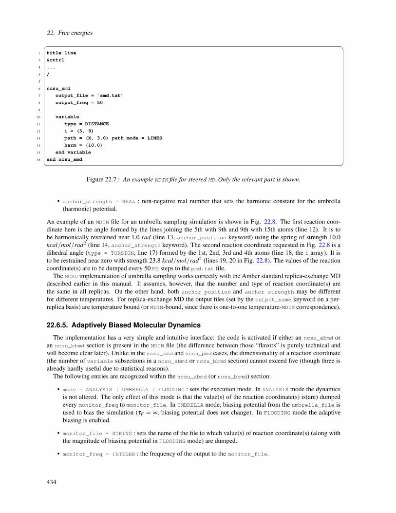
22. Free energies 1 title line
2 &cntrl
3 ...
4 /
5
6 ncsu_smd
7 output_file = ’smd.txt’
8 output_freq = 50
9
10 variable
11 type = DISTANCE
12 i = (5, 9)
13 path = (X, 3.0) path_mode = LINES
14 harm = (10.0)
15 end variable
16 end ncsu_smd Figure 22.7.: An example MDIN file for steered MD. Only the relevant part is shown.
• anchor_strength = REAL : non-negative real number that sets the harmonic constant for the umbrella(harmonic) potential.
An example of an MDIN file for an umbrella sampling simulation is shown in Fig. 22.8. The first reaction coor-dinate here is the angle formed by the lines joining the 5th with 9th and 9th with 15th atoms (line 12). It is tobe harmonically restrained near 1.0 rad (line 13, anchor_position keyword) using the spring of strength 10.0kcal/mol/rad2 (line 14, anchor_strength keyword). The second reaction coordinate requested in Fig. 22.8 is adihedral angle (type = TORSION, line 17) formed by the 1st, 2nd, 3rd and 4th atoms (line 18, the i array). It isto be restrained near zero with strength 23.8 kcal/mol/rad2 (lines 19, 20 in Fig. 22.8). The values of the reactioncoordinate(s) are to be dumped every 50 MD steps to the pmd.txt file.
The NCSU implementation of umbrella sampling works correctly with the Amber standard replica-exchange MDdescribed earlier in this manual. It assumes, however, that the number and type of reaction coordinate(s) arethe same in all replicas. On the other hand, both anchor_position and anchor_strength may be differentfor different temperatures. For replica-exchange MD the output files (set by the output_name keyword on a per-replica basis) are temperature bound (or MDIN-bound, since there is one-to-one temperature-MDIN correspondence).
22.6.5. Adaptively Biased Molecular Dynamics
The implementation has a very simple and intuitive interface: the code is activated if either an ncsu_abmd oran ncsu_bbmd section is present in the MDIN file (the difference between those “flavors” is purely technical andwill become clear later). Unlike in the ncsu_smd and ncsu_pmd cases, the dimensionality of a reaction coordinate(the number of variable subsections in a ncsu_abmd or ncsu_bbmd section) cannot exceed five (though three isalready hardly useful due to statistical reasons).
The following entries are recognized within the ncsu_abmd (or ncsu_bbmd) section:
• mode = ANALYSIS | UMBRELLA | FLOODING : sets the execution mode. In ANALYSIS mode the dynamicsis not altered. The only effect of this mode is that the value(s) of the reaction coordinate(s) is(are) dumpedevery monitor_freq to monitor_file. In UMBRELLA mode, biasing potential from the umbrella_file isused to bias the simulation (τF = ∞, biasing potential does not change). In FLOODING mode the adaptivebiasing is enabled.
• monitor_file = STRING : sets the name of the file to which value(s) of reaction coordinate(s) (along withthe magnitude of biasing potential in FLOODING mode) are dumped.
• monitor_freq = INTEGER : the frequency of the output to the monitor_file.
434

22.6. Adaptively biased MD, steered MD, and umbrella sampling with REMD 1 title line
2 &cntrl
3 ...
4 /
5
6 ncsu_pmd
7 output_file = ’pmd.txt’
8 output_freq = 50
9
10 variable ! first
11 type = ANGLE
12 i = (5, 9, 15)
13 anchor_position = 1.0
14 anchor_strength = 10.0
15 end variable
16 variable # second
17 type = TORSION
18 i = (1, 2, 3, 4)
19 anchor_position = 0.0
20 anchor_strength = 23.8
21 end variable
22 end ncsu_pmd Figure 22.8.: An example MDIN file for umbrella sampling (only relevant part is presented in full).
• timescale = REAL : τF , the flooding timescale in picoseconds (only required in FLOODING mode).
• umbrella_file = STRING : biasing potential file name (the file must exist for the UMBRELLA mode).
In FLOODING mode, the variable subsections of the ncsu_abmd section must also contain the following entries:
• min = REAL : smallest desired value of the reaction coordinate (required, unless the reaction coordinate islimited from below).
• max = REAL : largest desired value of the reaction coordinate (required, unless the reaction coordinate islimited from above).
• resolution = REAL : the “spatial” resolution for the reaction coordinate.
To access the biasing potential files created in the course of FLOODING simulations, the ncsu-umbrella-slice
utility is provided (it prints a short description of itself if invoked with --help option).An example MDIN file for the ncsu_abmd flavor of ABMD is shown in the Fig. 22.9.The reaction coordinate is defined in lines 17, 18 as the distance between the 5th and 9th atoms (more than one
reaction coordinates might be requested by mere inclusion of additional variable subsections). The mode is set toFLOODING thus enabling the adaptive biasing with flooding timescale τF = 100ps (line 14). The region of interestof the reaction coordinate is specified to be between -1Åand 10Å(line 19) and the resolution is set to 0.5Å(line 20).The lower bound (-1Å) could have been omitted for DISTANCE variable: the default value of zero would be usedin such case. The code will try to load the biasing potential from the umbrella.nc file (line 12) and use it as thevalue of U(t|ξ ) at the beginning of the run. The biasing potential built in the course of simulation will be saved tothe same file (umbrella.nc) every time the RESTRT file is written. The ncsu-umbrella-slice utility can then beused to access its content. An MDIN file for the follow up biased run at equilibrium would look much like the oneshown in the Fig. 22.9, but with mode changed from FLOODING to UMBRELLA.
The ncsu_abmd code works correctly with replica-exchange (that is, for -rem flag set to 1). In such case themonitor and umbrella files are temperature-bound (unlike, e.g., MDOUT and MDCRD files that require post processing).If number of sander groups exceeds one (the flag -ng is greater than one) and -rem flag is set to zero, the code runsmultiple walkers ABMD. In both cases the number and type(s) of variable(s) must be the same across all replicas.
435
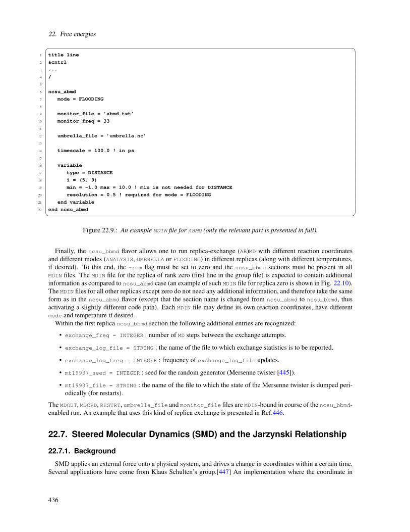
22. Free energies 1 title line
2 &cntrl
3 ...
4 /
5
6 ncsu_abmd
7 mode = FLOODING
8
9 monitor_file = ’abmd.txt’
10 monitor_freq = 33
11
12 umbrella_file = ’umbrella.nc’
13
14 timescale = 100.0 ! in ps
15
16 variable
17 type = DISTANCE
18 i = (5, 9)
19 min = -1.0 max = 10.0 ! min is not needed for DISTANCE
20 resolution = 0.5 ! required for mode = FLOODING
21 end variable
22 end ncsu_abmd Figure 22.9.: An example MDIN file for ABMD (only the relevant part is presented in full).
Finally, the ncsu_bbmd flavor allows one to run replica-exchange (AB)MD with different reaction coordinatesand different modes (ANALYSIS, UMBRELLA or FLOODING) in different replicas (along with different temperatures,if desired). To this end, the -rem flag must be set to zero and the ncsu_bbmd sections must be present in allMDIN files. The MDIN file for the replica of rank zero (first line in the group file) is expected to contain additionalinformation as compared to ncsu_abmd case (an example of such MDIN file for replica zero is shown in Fig. 22.10).The MDIN files for all other replicas except zero do not need any additional information, and therefore take the sameform as in the ncsu_abmd flavor (except that the section name is changed from ncsu_abmd to ncsu_bbmd, thusactivating a slightly different code path). Each MDIN file may define its own reaction coordinates, have differentmode and temperature if desired.
Within the first replica ncsu_bbmd section the following additional entries are recognized:
• exchange_freq = INTEGER : number of MD steps between the exchange attempts.
• exchange_log_file = STRING : the name of the file to which exchange statistics is to be reported.
• exchange_log_freq = INTEGER : frequency of exchange_log_file updates.
• mt19937_seed = INTEGER : seed for the random generator (Mersenne twister [445]).
• mt19937_file = STRING : the name of the file to which the state of the Mersenne twister is dumped peri-odically (for restarts).
The MDOUT, MDCRD, RESTRT, umbrella_file and monitor_file files are MDIN-bound in course of the ncsu_bbmd-enabled run. An example that uses this kind of replica exchange is presented in Ref.446.
22.7. Steered Molecular Dynamics (SMD) and the Jarzynski Relationship
22.7.1. Background
SMD applies an external force onto a physical system, and drives a change in coordinates within a certain time.Several applications have come from Klaus Schulten’s group.[447] An implementation where the coordinate in
436

22.7. Steered Molecular Dynamics (SMD) and the Jarzynski Relationship 1 title line
2 &cntrl
3 ...
4 /
5
6 ncsu_bbmd
7
8 ! 0th replica only
9
10 exchange_freq = 100 ! try for exchange every 100 steps
11
12 exchange_log_file = ’bbmd.log’
13 exchange_log_freq = 25
14
15 mt19937seed = 123455 ! random generator seed
16 mt19937file = ’mt19937.nc’ ! file to store/load the PRG
17
18 ! not specific for 0th replica
19
20 mode = ANALYSIS
21
22 monitorfile = ’bbmd.01.txt’ ! it is wise to have different
23 ! names in different replicas
24 monitor_freq = 123
25
26 variable
27 type = DISTANCE
28 i = (5, 9)
29 end variable
30 end ncsu_bbmd Figure 22.10.: An example MDIN file for ncsu_bbmd flavor of ABMD (only the relevant part is presented in full).
question changes in time at constant velocity is coded in this version of Amber. The present implementationhas been done by the group of Prof. Dario Estrin in Buenos Aires <[email protected]> by Marcelo Marti<[email protected]> and Alejandro Crespo <[email protected]>, and in the group of Prof. AdrianRoitberg at the University of Florida <[email protected]>.[448]
The method should be thought of as an umbrella sampling where the center of the restraint is time-dependent asin:
Vrest(t) = (1/2)k[x− x0(t)]2
where x could be a distance, an angle, or a torsion between atoms or groups of atoms.This methodology can be used then to drive a physical process such as ion diffusion, conformational changes and
many other applications. By integrating the force over time (or distance), a generalized work can be computed.This work can be used to compute free energy differences using the so-called Jarzynski relationship.[449–451]This method states that the free energy difference between two states A and B (differing in their values of thegeneralized coordinate x) can be calculated as
exp(−∆G/kBT ) = 〈exp(−W/kBT )〉A (22.14)
This means that by computing the work between the two states in question, and averaging over the initial state,equilibrium free energies can be extracted from non-equilibrium calculations. In order to make use of this feature,SMD calculations should be done, with different starting coordinates taken from equilibrium simulations. This can
437

22. Free energies
be done by running sander multiple times, or by running multisander (Section 18.11). There are examples of thevarious modes of action under the test/jar directories in the Amber distribution.
22.7.2. Implementation and usage
To set up a SMD run, set the jar variable in the &cntrl namelist to 1. The change in coordinates is performedfrom a starting to an end value in nstlim steps.
To specify the type and conditions of the restraint an additional ".RST" file is used as in nmropt=1. (Note thatjar=1 internally sets nmropt=1.) The restraint file is similar to that of NMR restraints (see Section 24.1), butfewer parameters are required. For instance, the following RST file could be used:
# Change distance between atoms 485 and 134 from 15 A to 20 A
&rst iat=485,134, r2=15., rk2 = 5000., r2a=20. /
Note that only r2,r2a and rk2 are required; rk3 and r3 are set equal to these so that the harmonic restraint is alwayssymmetric, and r1 and r4 are internally set so that the restrain is always operative. An SMD run changing an angle,would use three iat entries, and one changing a torsion needs four. As in the case of NMR restraints, group inputscan also be used, using iat<0 and defining the corresponding groups using the igr flag.
The output file differs substantially from that used in the case of nmr restraints. It contains 4 columns: x0(t), x,force, work. Here work is computed as the integrated force over distances (or angle, or torsion). These files can beused for later processing in order to obtain the free energy along the selected reaction coordinate using Jarzynski’sequality.
ExampleThe following example changes the distance between two atoms along 1000 steps:
Sample pulling input
&cntrl
nstlim=1000, cut=99.0, igb=1, saltcon=0.1,
ntpr=100, ntwr=100000, ntt=3, gamma_ln=5.0,
ntx=5, irest=1, ig = 256251,
ntc=2, ntf=2, tol=0.000001,
dt=0.002, ntb=0, tempi=300., temp0=300.,
jar=1,
/
&wt type=’DUMPFREQ’, istep1=1, /
&wt type=’END’, /
DISANG=dist.RST
DUMPAVE=dist_vs_t
LISTIN=POUT
LISTOUT=POUT Note that the flag jar is set to 1, and redirections to the dist.RST file are given. In this example the values in the
output file dist_vs_t are written every istep=1 steps.The restraint file dist.RST in this example is:
# Change distance between atoms 485 and 134 from 15 A to 20.0 A
&rst iat=485,134, r2=15., rk2 = 5000., r2a=20.0, /
and the output dist_vs_t file might contain:
15.00000 15.12396 -1239.55482 0.00000
15.00500 14.75768 2470.68119 3.07782
15.01000 15.13490 -1246.46571 6.13835
15.01500 15.15041 -1350.03026 -0.35289
15.02000 14.77085 2481.56731 2.47596
15.02500 15.12423 -987.34073 6.21152
15.03000 15.18296 -1520.41603 -0.05787
438

22.7. Steered Molecular Dynamics (SMD) and the Jarzynski Relationship
15.03500 14.79016 2431.22399 2.21915
.......
19.97000 19.89329 4.60255 67.01305
19.97500 19.87926 4.78696 67.03652
19.98000 19.86629 4.54839 67.05986
19.98500 19.85980 3.75589 67.08062
19.99000 19.86077 2.58457 67.09647
19.99500 19.86732 1.27678 67.10612
In this example, the work of pulling from 15.0 to 20.0 (over 2 ps) was 67.1 kcal/mol. One would need to repeatthis calculation many times, starting from different snapshots from an equilibrium trajectory constrained at theinitial distance value. This could be done with a long MD or a REMD simulation, and postprocessing with ptrajto extract snapshots. Once the work is computed, it should be averaged using Eq. 22.14 to get the final estimate ofthe free energy difference. The number of simulations, the strenght of the constraint, and the rate of change are allimportant factors. The user should read the appropriate literature before using this method. It is recommended thatthe width of the work distribution do not exceed 5-10% for faster convergence. In many cases, umbrella sampling(see Section 22.4) may be a better way to estimate the free energy of a conformational change.
439

23. Constant pH calculations
A constant pH molecular dynamics method was developed by John Mongan for simulations run with the Gener-alized Born implicit solvent model [452] and Jason Swails for simulations with explicit solvent. [453] Using eitherconstant pH method requires minor modifications to the process of generating the prmtop file and also requires asecond input file describing the titrating residues.
23.1. Background
Traditionally, molecular dynamics simulations have employed constant protonation states for titratable residues.This approach has many drawbacks. First, assigning protonation states requires knowledge of pKa values forthe protein’s titratable groups. Second, if any of these pKa values are near the solvent pH there may be no singleprotonation state that adequately represents the ensemble of protonation states appropriate at that pH. Finally, sinceprotonation states are constant, this approach decouples the dynamic dependence of pKa and protonation state onconformation.
The constant pH method implemented in sander and pmemd addresses these issues through Monte Carlo sam-pling of the Boltzmann distribution of protonation states concurrent with the molecular dynamics simulation. Theprotonation state distribution is affected by solvent pH, which is set as an external parameter. Residue protonationstates are changed by changing the partial charges on the atoms of the protonable residue.
23.2. Preparing a system for constant pH
Amber provides definitions for titrating side chains of ASP, GLU, HIS, LYS, TYR, and CYS. See below if youneed other titrating groups.
Begin by preparing your PDB file as you normally would for use with LEaP. Edit the PDB file, replacing allhistidine residue names (HIS, HID, or HIE) with HIP. Change all ASP and ASH to AS4 and all GLU and GLHto GL4. The others—LYS, TYR, and CYS—have the same name. This ensures that the prmtop file will have ahydrogen defined at every possible point of protonation. Note that these changes should only be applied to residuesthat you wish to titrate.
Run LEaP with the leaprc.constph command file. This file loads all parameters that were used for the referencecompounds. You can load this file with the following command:
source leaprc.constph
This loads the ff14SB force field. In addition, it loads the special carboxylate residue libraries and force fieldmodifications—constph.lib and frcmod.constph—that defines a hydrogen atom at each protonable location (syn-and anti- for both oxygens) along with improper torsions to prevent them from rotating into each other. It also setsthe GB solvation radii (PBradii) to mbondi2, which was the set used to parameterize the reference compounds.Now load your edited PDB file and proceed as usual to create the prmtop and prmcrd files. Changing any of theabove parameters should be closely checked by titrating the reference compounds and ensuring the predicted pKamatches.
Once you have the prmtop file, you need to generate a cpin file. The cpin file describes which residues shouldtitrate, and defines the possible protonation states and their relative energies. A python script, cpinutil.py, isprovided to generate this file. It takes a prmtop file as input, on the command line along with the GB model youwish to evaluate protonation transitions in, and writes the cpin file to STDOUT. Here is an example of generatingthe cpin file from your prmtop file, ’prmtop’ using the igb=2 GB model:
cpinutil.py -p prmtop -igb 2 > cpin
440
23.2. Preparing a system for constant pH
The cpinutil.py program accepts a number of flags that modify its behavior. By default, all residues start inprotonation state 0: deprotonated for ASP and GLU, protonated for LYS, TYR, and CYS, and doubly protonatedfor HIS (i.e. HIP). Initial protonation states can be specified using the -states flag followed by a comma and/orwhitespace-delimited list of initial protonation states (see below for more about protonation state definitions) asfollows:
cpinutil.py -p prmtop -igb 2 -states 1 3 0 0 0 1 > cpin
Note that if a list of states is provided, it must match exactly the number of residues that cpinutil has found totitrate based on the restrictions put on the command line. The -system flag can be used to provide a name for thetitrating system. This is purely cosmetic and has no effect on your simulations.
cpinutil.py -p prmtop -igb 2 -system HEWL > cpin
A number of flags are available for filtering which residues are included in the cpin file. All residues in the cpinfile, and only the residues in the cpin file, will be titrated. In general it is safe to exclude TYR and LYS for acidicsimulations and GL4 and AS4 for basic simulations. HIP should be included in all except very acidic simulations.Note that there is currently no support for titrating N or C terminal residues. If you have an N or C terminal residuewith a titratable sidechain, you should explicitly exclude it from the cpin file. The -resnum flag may be used tospecify which residue numbers should be retained; all others are deleted. Conversely, the -notresnum flag can beused to specify which residue numbers are deleted; all others are retained. Residue number refers to the numberingin the PDB file, not the index number among titrating residues. Similarly, -resname and -notresname can beused to filter by residue type. For instance, -notresname TYR,LYS would eliminate basic residues from the cpinfile. The -minpKa and -maxpKa flags can be used to filter out residues whose reference pKas do not satisfy thatcriteria. For example, -minpKa 5.0 will exclude all AS4 and GL4 residues from titrating.
You can get a full list of all available titratable residues using the --list argument to cpinutil.py, and you canget a full description of reference energies and charge vectors for any residue using the --describe argument.The full usage statement for cpinutil.py (accessible via -h/--help) is shown on the next page.
441

23. Constant pH calculations
usage: cpinutil.py [Options]
optional arguments:
-h, --help show this help message and exit
-v, --version show program’s version number and exit
-d, --debug Enable verbose tracebacks to debug this program
Output files:
-o FILE, --output FILE
Output file. Defaults to standard output
-op FILE, --output-prmtop FILE
For explicit solvent simulations, a custom set of
radii are necessary to obtain reasonable results for
carboxylate pKas (e.g., AS4 and GL4 residues). If
specified, this file will be the prmtop compatible
with the reference energies in the printed cpin file.
Required Arguments:
-p FILE Topology file to be used in constant pH simulation
Simulation Options:
-igb IGB Generalized Born model which you intend to use to
evaluate dynamics (or protonation state swaps).
Default is 2.
Residue Selection Options:
-resnames [RES [RES ...]]
Residue names to include in CPIN file
-notresnames [RES [RES ...]]
Residue names to exclude from CPIN file
-resnums [NUM [NUM ...]]
Residue numbers to include in CPIN file
-notresnums [NUM [NUM ...]]
Residue numbers to exclude from CPIN file
-minpKa pKa Minimum reference pKa to include in CPIN file
-maxpKa pKa Maximum reference pKa to include in CPIN file
System Information:
-states [NUM [NUM ...]]
List of default states to assign to titratable
residues
-system <system name>
Name of system to titrate. No effect on simulation.
Residue Information:
If any options here are used, no CPIN file will be written. These
arguments take precedence and are mutually exclusive with each other.
--describe [RESNAME [RESNAME ...]]
Print out the details of given residues
-l, --list List all titratable residues
This program will read a topology file and generate a cpin file for constant
pH simulations with sander
23.3. Running at constant pH
23.3.1. Running at constant pH in implicit solvent
Running constant pH simulations in either sander or pmemd has few differences from normal operation. In themdin file, you must set icnstph=1 to turn on constant pH in implicit solvent. solvph is used to set the solvent pH
442
23.3. Running at constant pH
value. You must also specify the period for Monte Carlo steps, ntcnstph (the number of steps between protonationstate change attempts). Note that only one residue is examined on each step, so you should decrease the step periodas the number of titrating residues increases to maintain a constant effective step period for each residue. We haveseen good results with fairly short periods, in the neighborhood of 100 fs effective period for each residue (e.g.ntcnstph=5, dt=0.002 with about 10 residues titrating).
Constant pH MD techniques employ a reference (model) compound to compute relative free energy differencesbetween the various protonation states through a thermodynamic cycle (see Figure 23.1). The free energy of theprotonation state change in the model compound that is necessary to yield the correct pKa is pre-computed foreach protonation state change. This so-called reference energy is printed to the cpin file by cpinutil.py. In orderto obtain sensible results, you must run your simulations with the same potential energy function for your systemthat was used to derive these reference energies (or alternatively rederive the reference energies with the potentialyou wish to use).
The reference energies were derived using the following parameters:
cut=30.0, igb=#, saltcon=0.1, nrespa=1,
temp0=300.0, ntc=2, ntf=2
where # is the value passed to the cpinutil.py program. In particular, care should be taken when modifying theigb, saltcon, nrespa, or temp0 parameters (nrespa should never be changed). The cutoff, 30 , is effectively infinitefor the (very small) model compounds, so using any reasonable cutoff—including an infinite cutoff—is valid. Theff99SB force field was used to parametrize the model compounds. Using other force fields should be validatedbefore you run simulations. If the charge scheme is the same as ff99SB (e.g., ff14SB), chances are good that thereference energies will still be valid. Other force fields (e.g., ff03 and ff13) that have different charge definitionsrequire recalculating the reference energies.
The model compounds have the sequence ACE-X-NME, where ACE is a neutral acetyl capping group, X is thetitratable residue, and NME is a neutral methylamine capping group. Both ACE and NME are provided in thestandard Amber residue libraries.
Some additional command line flags have been added to sander to support constant pH operation. The cpinfile must be specified using the -cpin option. Additionally, a history of the protonation states sampled is writtento the filename specified by -cpout. Finally, a constant pH restart file is written to the filename specified by -cprestrt. This is used to ensure that titrating residues retain the same protonation state when the simulation isrestarted. The constant pH restart file is a cpin-format file, and should be used as the cpin file when restarting thesimulation. It will generally be longer than the original cpin file, as it contains some amount of zeroed data. Theonly difference between the cprestrt file created at the end of a simulation and the cpin file used to start it will bethe RESSTATES array. Note that due to compiler-dependence of the namelist implementation, cprestrt files maydiffer from computer to computer.
443

23. Constant pH calculations
Figure 23.1.: Thermodynamic cycle used in CpHMD simulations. The energy difference between the two proto-nation states computed by sander is equal to the difference ∆G1−∆G2 and ∆GMC = ∆G2−∆G1−∆Gre f erence is used to evaluate the Metropolis Monte Carlo criteria for the proposed change in pro-tonation state(s).
23.3.2. Running at constant pH in explicit solvent
The hybrid molecular dynamics/Monte Carlo technique used in the implicit solvent calculations will not work inexplicit solvent because all protonation state changes will be opposed by the solvent orientation around the existingprotonation states. To work around this limitation while allowing MD to be propagated in explicit solvent, protona-tion state changes are still attempted using a Generalized Born implicit solvent model. [453] The workflow, shownin Figure 23.2, involves running MD for ntcnstph steps, stripping the solvent and ions, attempting protonationstate changes for each titratable residue in random order, and restoring the solvent for running solvent relaxationdynamics if any protonation states have changed before resuming MD.
The modifications needed to run explicit solvent simulations at constant pH are similar to the modificationsneeded to run implicit solvent simulations at constant pH, with some small differences highlighted here. Wefound that the existing GB radii defined for carboxylate oxygens is too large for the titratable residues AS4 andGL4. The reason is that the 4 hydrogen atoms in the carboxylate groups are all assigned an intrinsic solvent radiusthat contributes significantly to the effective radii of the carboxylate oxygens. To compensate, the intrinsic GBradii of AS4 and GL4 carboxylate oxygens must be reduced such that the effective radius is closer to thecarboxylate oxygen atoms of an ASP or GLU residue. The cpinutil.py script that generates the cpin file has beenmodified to make the necessary changes to the topology file (which can be written with the new “-op” flag thatwas added for this purpose). An example command-line used to set up a constant pH simulation in explicitsolvent for carboxylates is:
cpinutil.py -igb 2 -resnames AS4 GL4 -p <tleap_prmtop> \
444

23.4. Analyzing constant pH simulations
-op <new_radii_prmtop>
In the above command, new_radii_prmtop is generated and must be used for constant pH simulations. In additionto the modified topology file you need for CpHMD in explicit solvent, there is an additional parameter, ntrelax,that defines the number of solvent relaxation steps that will be performed following successful protonation statechanges. In general, we’ve found that while ca. 4 ps is required to generate a truly relaxed solvent distribution,200 fs is sufficient to account for the bulk of the solvent relaxation.
Another difference with respect to implicit CpHMD simulations is that a protonation state change attempt iscarried out for each residue in random order. This is done to allow protonation state change attempts to be donefar less frequently to limit the amount of MD time that is consumed by the solvent relaxation dynamics. Thefollowing input variables should be used in your sander or pmemd input file.
icnstph=2, ntcnstph=100, ntrelax=200,
solvph=6.4, saltcon=0.1, temp0=300.0,
ntc=2, ntf=2
Notice that the value of icnstph is 2, which indicates that CpHMD should be run in explicit solvent. The ntrelaxflag will run solvent relaxation dynamics (in which the non-solvent is held fixed) for 200 steps. The saltcon
variable controls the salt concentration for the GB calculations. It has no effect on the dynamics, but is requiredfor consistency with the reference energy of the model compound.
23.4. Analyzing constant pH simulations
As the simulation progresses, the protonation states that are sampled are written to the cpout file. A section of acpout file is included here:
Solvent pH: 2.00000
Monte Carlo step size: 2
Time step: 0
Time: 0.000
Residue 0 State: 1
Residue 1 State: 0
Residue 2 State: 1
Residue 3 State: 0
Residue 4 State: 1
Residue 5 State: 0
Residue 2 State: 0
Residue 4 State: 0
Residue 0 State: 3
Residue 1 State: 0
Residue 0 State: 0
One record is written on each Monte Carlo step. Each record is terminated by a blank line. There are two typesof records, full records and delta records. Full records, like the one shown above, lists the solvent pH, MC stepsize, current time step, and current time before listing every residue in the system. Full records are written on thefirst step and every ntwx steps afterwards so as to coincide with the frames written to the trajectory. Delta recordslist only those residues that were titrated (single or double lines for implicit solvent or a list of every residue forexplicit solvent). Note that in some cases, the protonation state for a delta record may be the same as that in anearlier record: this indicates that the Monte Carlo protonation move was rejected for that residue. The residuenumbers in cpout are indices over the titrating residues included in the cpin file; cpout files must be analyzed inconjunction with the cpin to map these indices back to the original system.
The Perl script calcpka.pl is provided in $AMBERHOME/AmberTools/src/etc as an example parser for the cpoutformat used for calculating predicted pKa values from cpout files. The cphstats program was written to replacecalcpka.pl. Its usage is described in Section 23.7.
445
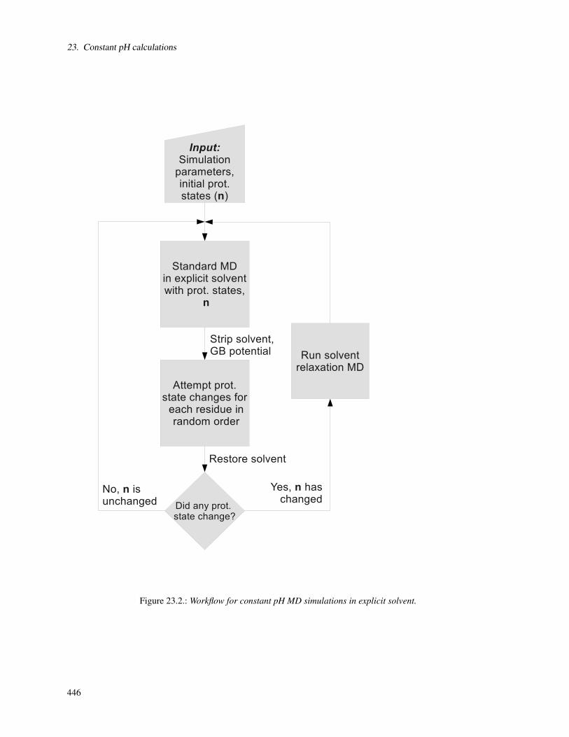
23. Constant pH calculations
Figure 23.2.: Workflow for constant pH MD simulations in explicit solvent.
446
23.5. Extending constant pH to additional titratable groups
23.5. Extending constant pH to additional titratable groups
There are two major components to defining a new titrating group for constant pH. First you must define thepartial charges for each atom in the residue for each protonation state. Then you must set the relative energies ofeach state.
Defining charge sets
Partial charges are most easily calculated using Antechamber and Gaussian. You must set up a model to cal-culate charges for each protonation state. If the titrating group you are defining is a polymer subunit (e.g. aminoacid residue), you must adjust the charges on atoms that have bonded interactions (including 1-4) with atoms inneighboring residues. The charges on these atoms must be changed so they are constant across all protonationstates - otherwise relative energies of protonation states become sequence dependent.cmmr an amino acid, thismeans that all backbone atoms must have constant charges. For the residues defined here, we arbitrarily selectedthe backbone charges of the protonated state to be used across all protonation states. The total charge differencebetween states should remain 1; we achieved this by adjusting the charge on the beta carbon.
Calculating relative energies
Relative energies are used to calibrate the method such that when a model compound is titrated at pH equal toits pKa, the energies (and thus populations) of the protonated and deprotonated states are equal.calcpkamalenergiesof the different protonation states are calculated using thermodynamic integration of a model compound betweenthe charge sets defined for the different protonation states. The model compound should be a small moleculethat mimics the bonded environment of the titratable group of interest, and for which experimental pK a data areavailable. For instance, the model compound for an amino acid X is generally ACE-X-NME; the model compoundfor a ligand might be the free ligand. The thermodynamic integration calculations must be performed using exactlythe same parameters and force field as you plan to use in your constant pH simulations. Once the relative energiesof the states are calculated by thermodynamic integration, the energy difference must be adjusted to account forthe pKa : the energy of the more protonated states should be increased by pKaRT ln(10).
For example suppose one were developing a model for an artificial amino acid, ART, with pK a 3.5 and twoprotonation states: ARP, having one proton and ARD having zero protons. After calculating partial charges asabove, you would construct a model compound having the sequence ACE-ARP-NME and generate a prmtop filewhere the ARP charges were perturbed to the ARD values (this can be done using the ParmEd program bundledwith AmberTools). You would then use sander to perform thermodynamic integration between ARP and ARD.Suppose that this showed that the energy of ARD relative to ARP was -6.3 kcal/mol. You would assign a relativeenergy of -6.3 to ARD and a relative energy of 3.5RTln(10) to ARP.
Testing the titratable group definitions
Prior to large scale use of your new titratable group definition, it’s a good idea to test it by performing aconstant pH simulation on your model compound, with pH set to the model pKa. Doing this requires generationof a cpin file, so this is a good time to define your titratable residue to to cpinutil.py. These definitions are foundin $AMBERHOME/AmberTools/src/parmed/parmed/amber/titratable_residues.py. The residue name must beadded to the list titratable_residues at the top of the file. Add your residue definition to the bottom of thefile, following the examples of the other residues (and make sure to execute the “check” function on that residueat the end as a way of checking your input. It is also a good idea to use cpinutil.py with --describe to check thatthe charge vectors match what you meant to input—the output format using --describe is much easier to checkthan the input in titratable_residues.py. The definition of CYS is shown below as an example.
# Cysteine
refene1 = _ReferenceEnergy(igb2=77.4666763, igb5=76.2588331, igb8=71.5804519)
refene1.solvent_energies(igb2=77.6041407, igb5=76.2827217)
refene1.set_pKa(8.5, deprotonated=False)
447

23. Constant pH calculations
refene2 = _ReferenceEnergy(igb2=0, igb5=0, igb8=0)
refene2.solvent_energies()
CYS = TitratableResidue(’CYS’, [’N’, ’H’, ’CA’, ’HA’, ’CB’, ’HB2’, ’HB3’, ’SG’,
’HG’, ’C’, ’O’], pka=8.5)
CYS.add_state(protcnt=1, refene=refene1, # protonated
charges=[-0.4157, 0.2719, 0.0213, 0.1124, -0.1231, 0.1112, 0.1112,
-0.3119, 0.1933, 0.5973, -0.5679])
CYS.add_state(protcnt=0, refene=refene2, # deprotonated
charges=[-0.4157, 0.2719, 0.0213, 0.1124, -0.3593, 0.1122, 0.1122,
-0.8844, 0.0, 0.5973, -0.5679])
CYS.check()
Reference energies are those calculated from TI (and adjusted if necessary to reproduce experimental pKas). Thereference energies should be calculated for all GB models you plan to support. For all but one of the states, setthe pKa of the residue so that the reference energy is properly adjusted to the given pKa. If the state to whichyou are applying that reference energy is protonated, then set deprotonated=False, as shown above. Otherwise, setdeprotonated=True.
You should always titrate your model compound to make sure that calculated pKas for the model compoundmatch experiment. The TI values are typically sufficient, but some residues may require adjustments.
23.6. Constant pH MD Replica Exchange
Running constant pH replica exchange simulations can be performed in either implicit or explicit solvent. Thereis no difference in the replica exchange setup between running in implicit or explicit solvent. This method isdescribed in Section 22.5.6 above. We have found that pH-REMD dramatically improves protonation state andconformational state sampling, so we suggest using it whenever possible.
23.7. cphstats
The cphstats command-line program was written by Jason Swails to compute protonation state statistics fromconstant pH simulations (in both implicit and explicit solvent). Written in C++, it is between one and two ordersof magnitude faster than the original calcpka.pl script written in Perl and roughly twice as fast as the calcpkaprogram written in Fortran 90. You can access a list and description of all available command-line flags using the--help flag, whose output is shown below.
Usage: cphstats [-O] [-V] [-h] [-i <cpin>] [-t] [-o FILE] [-R FILE -r INT]
[--chunk INT --chunk-out FILE] [--cumulative --cumulative-out FILE]
[-v INT] [-n INT] [-p|-d] [--calcpka|--no-calcpka] [--fix-remd]
[--population FILE] [-c CONDITION -c CONDITION -c ...]
[--conditional-output FILE] [--chunk-conditional FILE]
cpout1 [cpout2 [cpout3 ...] ]
General Options:
-h, --help Print this help and exit.
-V, --version Print the version number and exit.
-O, --overwrite
Allow existing outputs to be overwritten.
--debug Print out information about the files that are
being read in and used for the calculations.
--expert I will consider you an expert user and NOT warn
you if you try to compute statistics from REMD-based
files before using --fix-remd [NOT default behavior]
--novice I will warn you if you try to use REMD-based files
to compute statistics. [Default behavior]
Input Files and Options:
448

23.7. cphstats
-i FILE, --cpin FILE
Input cpin file (from sander) with titrating residue
information.
-t FLOAT, --time-step FLOAT
This is the time step in ps you used in your simulations.
It will be used to print data as a function of time.
Default is 2 fs (0.002)
Output Files:
-o FILE, --calcpka-output FILE
File to which the standard ‘calcpka’-type statistics
are written. Default is stdout
-R FILE, --running-avg-out FILE
Output file where the running averages of time series
data for each residue is printed (see [Output Options]
below for details). Default is [running_avgs.dat]
--chunk-out FILE
Output file where the time series data calculated
over chunks of the simulation are printed (see
[Output Options] below for details).
Default is [chunk.dat]
--cumulative-out FILE
Output file where the cumulative time series data
is printed (see [Output Options] below for details).
Default is [cumulative.dat]
--population FILE
Output file where protonation state populations are
printed for every state of every residue.
--conditional-output FILE
Output file with requested conditional probabilities.
Default is [conditional_prob.dat].
--chunk-conditional FILE
Prints a time series of the conditional probabilities over
a trajectory split up into chunks.
Output Options:
These options modify how the output files will appear
-v INT, --verbose INT
Controls how much information is printed to the
calcpka-style output file. Options are:
(0) Just print fraction protonated. [Default]
(1) Print everything calcpka prints.
-n INT, --interval INT
An interval between which to print out time series data
like ‘chunks’, ‘cumulative’ data, and running averages.
It is also used as the ’window’ of the conditional
probability time series (--chunk-conditional).
Default [1000]
-p, --protonated
Print out protonation fraction instead of deprotonation
fraction in time series data (Default behavior).
-d, --deprotonated
Print out deprotonation fraction instead of protonation
fraction in time series data.
-a, --pKa Print predicted pKas (via Henderson-Hasselbalch) in place
of fraction (de)protonated. NOT default behavior.
Analysis Options:
These options control which analyses are done. By default, only
the original, calcpka-style analysis is done.
449

23. Constant pH calculations
--calcpka Triggers the calcpka-style output [On by default]
--no-calcpka Turns off the calcpka-style output
-r WINDOW, --running-avg WINDOW
Defines a window size for a moving, running average
time series. <WINDOW> is the number of MD steps (NOT
the number of MC exchange attempts).
--chunk WINDOW
Computes the time series data over a chunk of the
simulation of size <WINDOW> time steps. See above for
details.
--cumulative Computes the cumulative average time series data (see above
for options) over the course of the trajectory.
--fix-remd PREFIX
This option will trigger cphstats to reassemble the
titration data into pH-specific ensembles. This
is an exclusive mode of the program---no other
analyses will be done.
-c CONDITIONAL, --conditional CONDITIONAL
Evaluates conditional probabilities. CONDITIONAL should be a
string of the format:
<resid>:<state>,<resid>:<state>,...
or
<resid>:PROT,<resid>:DEPROT,...
or
<resid>:<state1>;<state2>,<resid>:PROT,...
Where <resid> is the residue number in the prmtop (NOT the
cpin) and <state> is either the state number or (p)rotonated
or (d)eprotonated, case-insensitive
This program analyzes constant pH output files (cpout) from Amber.
These output files can be compressed using gzip compression. The
compression will be detected automatically by the file name extension.
You must have the gzip headers for this functionality to work.
23.7.1. Standard statistics
The standard output of cphstats is the same as that for the calcpka and calcpka.pl programs that camebefore. An example from a protein with 10 titratable residues is shown below.
Solvent pH is 4.000
GL4 7 : Offset -0.448 Pred 3.552 Frac Prot 0.263 Transitions 91163
HIP 15 : Offset 2.036 Pred 6.036 Frac Prot 0.991 Transitions 6194
AS4 18 : Offset -1.063 Pred 2.937 Frac Prot 0.080 Transitions 41490
GL4 35 : Offset 2.113 Pred 6.113 Frac Prot 0.992 Transitions 5458
AS4 48 : Offset -1.365 Pred 2.635 Frac Prot 0.041 Transitions 17596
AS4 52 : Offset -1.123 Pred 2.877 Frac Prot 0.070 Transitions 25306
AS4 66 : Offset -1.689 Pred 2.311 Frac Prot 0.020 Transitions 7334
AS4 87 : Offset -1.757 Pred 2.243 Frac Prot 0.017 Transitions 8976
AS4 101 : Offset 0.342 Pred 4.342 Frac Prot 0.687 Transitions 105377
AS4 119 : Offset -1.894 Pred 2.106 Frac Prot 0.013 Transitions 6700
Average total molecular protonation: 4.174
The external pH that was set in sander or pmemd is shown at the top, followed by each of the residues with theirname and number as they appear in the topology file. The computed pKa values printed by cphstats are computedby fitting to the Hendersen-Hasselbalch equation (Eq. 23.1). The values printed in the standard output are definedbelow:
Offset Difference in pK units that the predicted pKa is from the solvent pH.
450

23.7. cphstats
Pred The predicted pKa computed from the fraction protonated and the pH in Eq. 23.1.
Frac Prot The total fraction of the simulation that the residue spent in its ‘protonated’ form.
Transitions The number of times that the total number of ‘active’ protons on the titratable residue changed fol-lowing a protonation state change attempt. This does not count when the protonation state changed betweentwo tautomers or protomers with the same number of protons. For instance, the switching from the HIDto the HIE tautomers of histidine does not count. Nor does switching from the syn-O1-protonated to thesyn-O2-protonated forms of any carboxylate residues.
pKa = pH− log(
1− fp
fp
)(23.1)
In Eq. 23.1, fp is the total fraction protonated for a given residue. A more rigorous way of computing the pKaof a titratable residue is to fit Eq. 23.2—the Hill equation—to the pHs and protonation fractions collected overa full titration curve to compute the best-fit values of the Hill coefficient (n) and computed pKa. This requirespost-processing the output from cphstats with your own script or program.
fd = 1− fp =1
1+10n(pKa−pH)(23.2)
Example You can analyze as many cpout files as you would like, provided that each cpout file was generatedfrom a simulation run at the same pH as the others. For pH-REMD simulations, a pre-processing stage is initiallyrequired, as described in a section 23.7.5. You can direct cphstats to print the output to a file with the -o flag orhave it printed to the screen (stdout) by default. You must provide a cpin file with the -i flag to calculate anyprotonation state statistics.
cphstats -i cpin pH_4.md1.cpout pH_4.md2.cpout pH_4.md3.cpout \
-o pH_4.dat
23.7.2. Cumulative, running, and “chunk” averages
These options provide a way of monitoring how the ensemble of protonation states evolve during the course ofa simulation. Because MD yields insights into the dynamical behavior of molecules, it’s often advantageous tomonitor the evolution of the protonation state fractions with geometric measurements of the system coordinates.Each option—cumulative, running, and “chunk” averages—can be output as a time series of fraction protonated,fraction deprotonated, or predicted pKa using the -p, -d, and -a flags, respectively. The details of calculatingeach of these properties is described in the next sections. The output is printed to a file in the following format:
#Time step GL4 7 HIP 15 AS4 18 GL4 35 Total Avg. Prot.
1000 0.30693 0.99505 0.00000 0.99505 3.900498
2000 0.24378 0.99751 0.00000 0.99751 3.962594
3000 0.23754 0.99834 0.05150 0.99834 4.014975
...
The final column is always the total average protonation (note, a protonated histidine counts as ‘2’ protons and aprotonated lysine counts as ‘3’, so only differences in total protonation fraction are meaningful). The time stepcorresponds to the actual MD time step, not the interval between protonation state changes.
Cumulative averages
A cumulative average is a time series whose values at time t are calculated according to
〈A〉t =∫ t
0 A(t)dtt
such that it represents the average value from time 0 to t. The final average should match the output printed inthe standard statistics output of the previous section, which is an average over the entire ensemble. Cumulative
451

23. Constant pH calculations
averages can be misleading, however, as 〈A〉t changes rapidly when t is small and very slowly as t becomes large.It can give the impression that a property is converging to a particular value when in fact that property is fluctuatinga lot.
Example To compute a cumulative average, you must use the --cumulative flag to indicate you wish tocompute this value. You can control how frequently this quantity is sampled by setting the interval, in MD timesteps (not protonation state change attempts), using the -n flag. The default interval is to print values every 1000time steps. The longer your simulation is, the less frequently you have to sample points. Data is written to the filecumulative.dat unless a different name is provided with the --cumulative-out flag. An example usage is:
cphstats -i cpin pH_4.md1.cpout pH_4.md2.cpout pH_4.md3.cpout -n 10000 -p \
--no-calcpka --cumulative --cumulative-out pH_4_cumulative.dat
The --no-calcpka flag prevents the standard statistics (previous section) from being computed and printed. Thecumulative protonated fraction will be printed to the file pH_4_cumulative.dat with values dumped every 10000steps.
Running averages
A running average is a time series whose values at time t are calculated according to
〈A〉t =∫ t+σ
t−σA(t)dt
2σ
such that it represents the average value from t−σ to t+σ—the value 2σ is referred to as the window size. Theadvantage of a running average over a cumulative average is that the shape of the curve at large values of t do notdepend on the values near t = 0. If the interval is smaller than the window size, then adjacent values of 〈A〉t willbe comprised of overlapping data points.
Example To compute a running average, you must specify a window size, in MD time steps, with the -r flag.The interval—specified with the -n flag—controls how frequently samples from the time series are saved to theoutput file. An example usage is
cphstats -i cpin pH_4.md1.cpout pH_4.md2.cpout pH_4.md3.cpout \
-n 2000 -r 10000 -R pH_4_runningavg.dat -d
This command will compute the running average of the deprotonation fraction (because of the -d flag) every 2000time steps with a window size of 10000 time steps—the average will be computed from the 5000 steps beforetime t to 5000 steps after time t every 2000 steps. It may be important to note that any portion of the window thatextends before t = 0 or after the last time step of the simulation is simply truncated. In this example, the runningaverage data is printed to the file pH_4_runningavg.dat and the standard statistical output is printed to the screen.
“Chunk” averages
A “chunk” average is a time series in which the trajectory is segmented into separate chunks of specified size2σ time steps. The average value is then calculated according to
〈A〉t =∫ t+σ
t−σA(t)dt
2σ
Indeed, “chunk” averages are simply a special case of running averages in which the times for which 〈A〉t arecomputed are the center points of the time chunks. In this analysis, every point of the simulation is uniquelyassigned to a single chunk (so no overlap is possible like there is for running averages with a window size largerthan twice the interval).
452
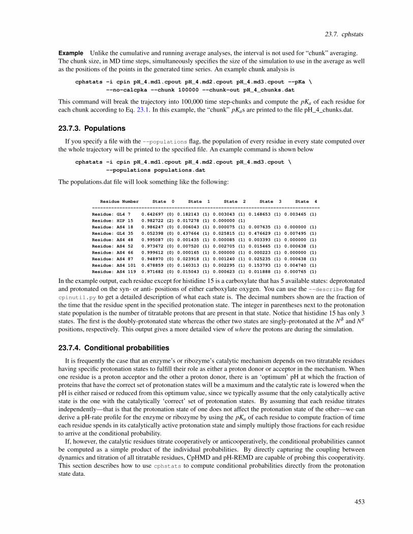
23.7. cphstats
Example Unlike the cumulative and running average analyses, the interval is not used for “chunk” averaging.The chunk size, in MD time steps, simultaneously specifies the size of the simulation to use in the average as wellas the positions of the points in the generated time series. An example chunk analysis is
cphstats -i cpin pH_4.md1.cpout pH_4.md2.cpout pH_4.md3.cpout --pKa \
--no-calcpka --chunk 100000 --chunk-out pH_4_chunks.dat
This command will break the trajectory into 100,000 time step-chunks and compute the pKa of each residue foreach chunk according to Eq. 23.1. In this example, the “chunk” pKas are printed to the file pH_4_chunks.dat.
23.7.3. Populations
If you specify a file with the --populations flag, the population of every residue in every state computed overthe whole trajectory will be printed to the specified file. An example command is shown below
cphstats -i cpin pH_4.md1.cpout pH_4.md2.cpout pH_4.md3.cpout \
--populations populations.dat
The populations.dat file will look something like the following:
Residue Number State 0 State 1 State 2 State 3 State 4
-----------------------------------------------------------------------------------
Residue: GL4 7 0.642697 (0) 0.182143 (1) 0.003043 (1) 0.168653 (1) 0.003465 (1)
Residue: HIP 15 0.982722 (2) 0.017278 (1) 0.000000 (1)
Residue: AS4 18 0.986247 (0) 0.006043 (1) 0.000075 (1) 0.007635 (1) 0.000000 (1)
Residue: GL4 35 0.052398 (0) 0.437664 (1) 0.025815 (1) 0.476629 (1) 0.007495 (1)
Residue: AS4 48 0.995087 (0) 0.001435 (1) 0.000085 (1) 0.003393 (1) 0.000000 (1)
Residue: AS4 52 0.973672 (0) 0.007520 (1) 0.002705 (1) 0.015465 (1) 0.000638 (1)
Residue: AS4 66 0.999612 (0) 0.000165 (1) 0.000000 (1) 0.000223 (1) 0.000000 (1)
Residue: AS4 87 0.948970 (0) 0.023918 (1) 0.001240 (1) 0.025235 (1) 0.000638 (1)
Residue: AS4 101 0.678859 (0) 0.160313 (1) 0.002295 (1) 0.153793 (1) 0.004740 (1)
Residue: AS4 119 0.971682 (0) 0.015043 (1) 0.000623 (1) 0.011888 (1) 0.000765 (1)
In the example output, each residue except for histidine 15 is a carboxylate that has 5 available states: deprotonatedand protonated on the syn- or anti- positions of either carboxylate oxygen. You can use the --describe flag forcpinutil.py to get a detailed description of what each state is. The decimal numbers shown are the fraction ofthe time that the residue spent in the specified protonation state. The integer in parentheses next to the protonationstate population is the number of titratable protons that are present in that state. Notice that histidine 15 has only 3states. The first is the doubly-protonated state whereas the other two states are singly-protonated at the Nδ and Nε
positions, respectively. This output gives a more detailed view of where the protons are during the simulation.
23.7.4. Conditional probabilities
It is frequently the case that an enzyme’s or ribozyme’s catalytic mechanism depends on two titratable residueshaving specific protonation states to fulfill their role as either a proton donor or acceptor in the mechanism. Whenone residue is a proton acceptor and the other a proton donor, there is an ‘optimum’ pH at which the fraction ofproteins that have the correct set of protonation states will be a maximum and the catalytic rate is lowered when thepH is either raised or reduced from this optimum value, since we typically assume that the only catalytically activestate is the one with the catalytically ‘correct’ set of protonation states. By assuming that each residue titratesindependently—that is that the protonation state of one does not affect the protonation state of the other—we canderive a pH-rate profile for the enzyme or ribozyme by using the pKa of each residue to compute fraction of timeeach residue spends in its catalytically active protonation state and simply multiply those fractions for each residueto arrive at the conditional probability.
If, however, the catalytic residues titrate cooperatively or anticooperatively, the conditional probabilities cannotbe computed as a simple product of the individual probabilities. By directly capturing the coupling betweendynamics and titration of all titratable residues, CpHMD and pH-REMD are capable of probing this cooperativity.This section describes how to use cphstats to compute conditional probabilities directly from the protonationstate data.
453

23. Constant pH calculations
Conditional Probability Expressions
This section describes the syntax of the conditional probability expressions that you must use for cphstats.The format of the expression is a comma-delimited list of residue:state specifications shown below.
<residue 1>:<state specification>,<residue 2>:<state specification>
You can list as many residues as you want. A snapshot satisfies the conditional probability criteria if each of thespecified residues is in the list of allowable states within the state specifications—unspecified residues can be inany state. The residue specifiers are the residue numbers in the topology file. The state specification can be eithera semicolon-delimited list of state numbers or the description “protonated” or “deprotonated.” The parser iscase-insensitive and you only have to type up to one letter of either word to trigger recognition of “protonated” or“deprotonated.” Example conditional probability expressions are shown below with accompanying descriptionsof what conditional probabilities they define. Individual residue:state specifications are indicated by color.
“35:P,52:D”
This expression is satisfied if residue 35 is protonated at the same time that residue 52 is deprotonated.
“35:Prot,52:1;3,15:1”
This expression is satisifed if residue 35 is protonated and residue 52 is in either state 1 or 3 and residue 15 is instate 1. Other residues can be in any state.
Examples
You can specify conditional probability expressions following the -c flag on the command-line. You canspecify as many expressions as you want, as long as each one is preceded by -c or --conditional. The fractionof states that satisfy each conditional probability is written to the conditional probability output file specified by--conditional-output (or conditional_prob.dat by default). An example command-line is shown below
cphstats -i cpin pH_4.md1.cpout pH_4.md2.cpout pH_4.md3.cpout \
-c “35:P,52:D” -c “35:prot,52:1;3,15:1” \
--conditional-output conditional.dat
Example output from conditional.dat is shown below.
Conditional Probabilities Fraction
35:P,52:D 0.982922
35:prot,52:1;3,15:1 0.000290
For the sake of comparison, the standard statistics are shown below.
Solvent pH is 4.000
GL4 7 : Offset -0.167 Pred 3.833 Frac Prot 0.405 Transitions 31378
HIP 15 : Offset 1.391 Pred 5.391 Frac Prot 0.961 Transitions 5578
AS4 18 : Offset -1.851 Pred 2.149 Frac Prot 0.014 Transitions 1910
GL4 35 : Offset 2.432 Pred 6.432 Frac Prot 0.996 Transitions 391
AS4 48 : Offset -2.282 Pred 1.718 Frac Prot 0.005 Transitions 570
AS4 52 : Offset -1.855 Pred 2.145 Frac Prot 0.014 Transitions 438
AS4 66 : Offset -1.998 Pred 2.002 Frac Prot 0.010 Transitions 698
AS4 87 : Offset -1.489 Pred 2.511 Frac Prot 0.031 Transitions 1239
AS4 101 : Offset -0.478 Pred 3.522 Frac Prot 0.250 Transitions 19924
AS4 119 : Offset -1.516 Pred 2.484 Frac Prot 0.030 Transitions 2408
Average total molecular protonation: 3.716
In this example, residue 35 is protonated while residue 52 is deprotonated 98.2922% of the time. Assuming thatthe two residues titrate independently, we would calculate this conditional probability to be 0.996× (1−0.014)×100% = 98.2056%. This indicates that these residues titrate independently at pH 4.
454

23.7. cphstats
Conditional probability “chunks”
cphstats currently supports creating time series of conditional probabilities by breaking the trajectory intoequal-sized “chunks” and computing the conditional probability over that chunk (see Sec. 23.7.2 for details). Toperform this analysis, specify a conditional “chunk” output file with the --chunk-conditional flag. The -n flagis used to define the size of the chunk (the same flag used to define the time series interval for cumulative andrunning averages). The format of the output file is the same as that shown in Sec. 23.7.2 for the other time series,but the columns are labeled with the conditional probability expression instead of the residue name and number.An example usage is shown below.
cphstats -i cpin pH_4.md1.cpout pH_4.md2.cpout pH_4.md3.cpout \
-c “35:P,52:D” -c “35:prot,52:1;3,15:1” -n 100000 \
--chunk-conditional chunk_conditional.dat
This example will break the simulation into 100,000-time-step chunks and compute the two conditional probabili-ties over each chunk, writing the results to chunk_conditional.dat.
23.7.5. Processing pH-REMD cpout files
Replica exchange in pH-space is performed by attempting to exchange solution pH between replicas. Likewith temperature-based REMD, this means that individual replicas do not keep the same pH throughout the entiresimulation. Since many of the analyses described in the previous sections pertain to ensembles at one pH, theyare not readily applicable to the raw output from pH-REMD simulations and must often be pre-processed beforebeing analyzed. This section describes only how to do the preprocessing. You are expected to be familiar with thecontent of Subsection 22.5.6 above.
Re-ordering cpout files
You can use cphstats to generate pH-specific cpout files from pH-REMD replica cpout files using the--fix-remd flag. To do so, you must provide a file name prefix to which the suffix .pH_X will be appended aswell as the cpout files from every replica for a single simulation (and only a single simulation). If you ran thesimulation in multiple steps, using restarts from the previous simulation to start the next, you will have to run thecommand described here for each segment of the total simulation separately. No cpin file is needed for this step.An example usage is shown below:
cphstats --fix-remd cpout pH_1.md1.cpout pH_2.md1.cpout pH_3.md1.cpout \
pH_4.md1.cpout pH_5.md1.cpout pH_6.md1.cpout
This command will create the files cpout.pH_1.00, cpout.pH_2.00, cpout.pH_3.00, cpout.pH_4.00, cpout.pH_5.00,and cpout.pH_6.00 that can subsequently be used for the analyses described in the previous section.
If you attempt to use REMD cpout files without fixing them in the previous analyses, you will receive an error.
Analyzing replica statistics
There are times when you may want to analyze statistics, such as fraction protonated or deprotonated, from asingle replica when looking at things like correlation times, for instance. You can disable the REMD file protectionusing the --expert flag, but note that any computed pKa is based on Eq. 23.1 with a single pH, so they will bemeaningless for REMD-based trajectories.
455
24. NMR, X-ray, and cryo-EM/ET refinement
We find the sander module to be a flexible way of incorporating a variety of restraints into a optimizationprocedure that includes energy minimization and dynamical simulated annealing. The "standard" sorts of NMRrestraints, derived from NOE and J-coupling data, can be entered in a way very similar to that of programs likeDISGEO, DIANA or X-PLOR; an aliasing syntax allows for definitions of pseudo-atoms, connections with peaknumbers in spectra, and the use of "ambiguous" constraints from incompletely-assigned spectra. More "advanced"features include the use of time-averaged constraints, use of multiple copies (LES) in conjunction with NMRrefinement, and direct refinement against NOESY intensities, paramagnetic and diamagnetic chemical shifts, orresidual dipolar couplings. In addition, a key strength of the program is its ability to carry out the refinements(usually near the final stages) using an explicit-solvent representation that incorporates force fields and simulationprotocols that are known to give pretty accurate results in many cases for unconstrained simulations; this abilityshould improve predictions in regions of low constraint density and should help reduce the number of places wherethe force field and the NMR constraints are in "competition" with one another.
Since there is no generally-accepted "recipe" for obtaining solution structures from NMR data, the commentsbelow are intended to provide a guide to some commonly-used procedures. Generally speaking, the programs thatneed to be run to obtain NMR structures can be divided into three parts:
1. front-end modules, which interact with NMR databases that provide information about assignments, chemi-cal shifts, coupling constants, NOESY intensities, and so on. We have tried to make the general format of theinput straightforward enough so that it could be interfaced to a variety of programs. At TSRI, we generallyuse the FELIX and NMRView codes, but the principles should be similar for other ways of keeping trackof a database of NMR spectral information. As the flow-chart on the next page indicates, there are only afew files that need to be created for NMR restraints; these are indicated by the solid rectangles. The primarydistance and torsion angle files have a fairly simple format that is largely compatible with the DIANA pro-grams; if one wishes to use information from ambiguous or overlapped peaks, there is an additional "MAP"file that makes a translation from peak identifiers to ambiguous (or partial) assignments. Finally, there aresome specialized (but still pretty straightforward) file formats for chemical shift or residual dipolar couplingrestraints.
There are a variety of tools, besides the ones described below, that can assist in preparing input for structurerefinement in Amber.
• The SANE (Structure Assisted NOE Evaluation) package, http://ambermd.org/sane.zip, is widely usedat The Scripps Research Institute.[454]
• If you use Bruce Johnson’s NmrView package, you might also want to look at the TSRI additions tothat: http://garbanzo.scripps.edu/nmrgrp/wisdom/pipe/tips_scripts.html. In particular, the xpkTOupland starTOupl scripts there convert NmrView peak lists into the "7-column" needed for input tomakeDIST_RST.
• Users of the MARDIGRAS programs from UCSF can use the mardi2amber program to do conversionto Amber format: http://picasso.ucsf.edu/mardihome.html
2. restrained molecular dynamics, which is at the heart of the conformational searching procedures. This is thepart that sander itself handles.
3. back-end routines that do things like compare families of structures, generate statistics, simulate spectra,and the like. For many purposes, such as visualization, or the running of procheck-NMR, the "interface"to such programs is just the set of PDB files that contain the family of structures to be analyzed. Thesegeneral-purpose structure analysis programs are available in many locations and are not discussed here. The
456

24.1. Distance, angle and torsional restraints
principal sander-specific tool is sviol, which prepares tables and statistics of energies, restraint violations,and the like.
24.1. Distance, angle and torsional restraints
Distance, angle, and other restraints are read from the DISANG file if nmropt > 0. Namelist rst ("&rst")contains the following variables; it is read repeatedly until a namelist &rst statement is found with IAT(1)=0, oruntil reaching the end of the DISANG file.
[In many cases, the user will nkot prepare this section of the input by hand, but will use the auxiliary programsmakeDIST_RST, makeANG_RST and makeCHIR_RST to prepare input from simpler files. See also the programscyanarest_to_amberRST and nef_to_RST if you have restraints in Cyana or NEF (NMR Exchange Format) for-mats.]
24.1.1. Variables in the &rst namelist:
iat(1)→iat(8)
• If IRESID = 0 (normal operation): The atoms defining the restraint. Type of restraint is determined (inorder) by:
1. If IAT(3) = 0, this is a distance restraint.
2. If IAT(4) = 0, this is an angle restraint.
3. If IAT(5) = 0, this is a torsional (or J-coupling, if desired) restraint or a genereralized distance restraintof 4 atoms, a type of restraint new as of Amber 10 (sander only, see below).
4. If IAT(6) = 0, this is a plane-point angle restraint, a second restraint new as of Amber 10 (sander only).The angle is measured between the normal of a plane defined by IAT(1)..IAT(4) and the vector fromthe center of mass of atoms IAT(1)..IAT(4) to the position of IAT(5). The normal is defined by (r1 - r2)× (r3 - r4), where rn is the position of IAT(n).
5. If IAT(7) = 0, this is a generalized distance restraint of 6 atoms (see below).
6. Otherwise, if IAT(1)..IAT(8) are all nonzero, this is a plane- plane angle restraint, a third new restrainttype as of Amber 10 (sander only, or a generalized distance restraint of 8 atoms (see below). For theplane-plane restraint, the angle is measured between the two normals of the two planes, which aredefined by (r1 - r2) × (r3 - r4) and (r5 - r6) × (r7 - r8). In the case of either planar restraint, the planemay be defined using three atoms instead of four simply by using one atom twice.
If any of IAT(n) are < 0, then a corresponding group of atoms is defined below, and the coordinate- averagedposition of this group will be used in place of atom IAT(n). A new feature as of Amber 10, atom groupsmay be used not only in distance restraints, but also in angle, torsion, the new plane restraints, or the newgeneralized restraints. If this is a distance restraint, and IAT1 <0, then a group of atoms is defined below, andthe coordinate-averaged position of this group will be used in place of the coordinates of atom 1 [IAT(1)].Similarly, if IAT(2) < 0, a group of atoms will be defined below whose coordinate-averaged position will beused in place of the coordinates for atom 2 [IAT(2)].
• If IRESID=1: IAT(1)..IAT(8) point to the *residues* containing the atoms comprising the internal. Residuenumbers are the absolute in the entire system. In this case, the variables ATNAM(1)..ATNAM(8) must bespecified and give the character names of the atoms within the respective residues. If any of IAT(n) are lessthan zero, then group input will still be read in place of the corresponding atom, as described below.
• Defaults for IAT(1)→IAT(8) are 0.
rstwt(1)→rstwt(4) New as of Amber 10 (sander only), users may now define a single restraint that is a function ofmultiple distance restraints, called a "generalized distance coordinate" restraint. The energy of such arestraint has the following form:
457

24. NMR, X-ray, and cryo-EM/ET refinement
U = k(w1|r1− r2|+w2|r3− r4|+w3|r5− r6|+w4|r7− r8|− r0)2
where the weights wnare given in rstwt(1)..rstwt(4) and the positions rnare the positions of the atomsin iat(1)..iat(8).
Generalized distance coordinate restraints must be defined with either 4, 6, or 8 atoms and 2, 3, or4 corresponding nonzero weights in rstwt(1)..rstwt(4). Weights may be any positive or negative realnumber.
If all the weights in rstwt(1)..rstwt(4) are zero and four atoms are given in iat(1)..iat(4) for the restraint,the restraint is a torsional or J-coupling restraint. If eight atoms are given in iat(1)..iat(8) and allweights are zero, the restraint is a plane-plane angle restraint. However, if the weights are nonzero,the restraint will be a generalized distance coordinate restraint.
Default for rstwt(1)..rstwt(4) is 0.0
restraint New as of Amber 10 (sander only), users may now use a "natural language" system to define restraintsby using the RESTRAINT character variable. Valid restraints defined in this manner will begin witha "distance( )" "angle( )" "torsion( )" or "coordinate( )" keyword. Within the parentheses, the atomsthat make up the restraint are specified. Atoms may be defined either with an explicit atom number orby using ambmask format, namely :(residue#)@(atom name). Atoms may be separated by commas,spaces, or parentheses. Additionally, negative integers may be used if atom groupings are defined inother variables in the namelist as described below. In addition to the principle distance, angle, torsion,and coordinate keywords, Some keywords may be used within the principle keywords to define morecomplicated restraints. The keyword "plane( )" may be used once or twice within the parentheses ofthe "angle( ) keyword to define a planar restraint. Defining one plane grouping plus one other atom inthis manner will create a plane-point angle restraint as described above. Defining two plane groupingswill create a plane-plane angle restraint. The keyword "plane( )" may only be used inside of "angle()," and is necessary to define either a plane-point or plane-plane restraint.Within the "coordinate( )" keyword, the user must use 2 to 4 "distance( )" keywords to define ageneralized distance coordinate restraint. The "distance( )" keyword functions just like it does whenused to define a traditional distance restraint. The user may specify any two atom numbers, masks,or negative numbers corresponding to atom groups defined outside of RESTRAINT. Additionally,following each "distance( )" keyword inside "coordinate( )" the user must specify a real-numberweight to be applied to each distance making up the generalized coordinate.The "com( )" keyword may be used within any other keyword to define a center of mass grouping ofatoms. Within the parenthesis, the user will enter a list of atom numbers or masks. Negative numbers,which correspond to externally-defined groups, may not be used.Any type of parenthetical character, i.e., ( ), [ ], or , may be used wherever parentheses have beenused above.
The following are all examples of valid restraint definitions:
restraint = "distance( (45) (49) )"
= "angle (:21@C5’ :21@C4’ 108)"
= "torsion[-1,-1,-1, com(67, 68, 69)]"
= "angle( -1, plane(81, 85, 87, 90) )"
= "angle(plane(com(9,10),:5@CA,31,32),plane(14,15,15,16))"
= "coordinate(distance(:5@C3’,:6@O5’),-1.0,distance(134,-1),1.0)"
There is a 256 character limit on RESTRAINT, so if a particularly large atom grouping is desired, it isnecessary to specify a negative number instead of "com( )" and define the group as described below.RESTRAINT will only be parsed if IAT(1) = 0, otherwise the information in IAT(1) .. IAT(8) willdefine the restraint. Default for restraint is ’ ’.
atnam If IRESID = 1, then the character names of the atoms defining the internal are contained inATNAM(1)→ATNAM(8). Residue IAT(1) is searched for atom name ATNAM(1); residue IAT(2)is searched for atom name ATNAM(2); etc. Defaults for ATNAM(1)→ATNAM(8) are ’ ’.
458
24.1. Distance, angle and torsional restraints
iresid Indicates whether IAT(I) points to an atom # or a residue #. See descriptions of IAT() and ATNAM()above. If RESTRAINT is used to define the internal instead of IAT(), IRESID has no effect on howRESTRAINT is parsed. However, it will affect the behavior of atom group definitions as describedbelow if negative numbers are specified within RESTRAINT. Default = 0.
nstep1, nstep2 This restraint is applied for steps/iterations NSTEP1 through NSTEP2. If NSTEP2 = 0, the restraintwill be applied from NSTEP1 through the end of the run. Note that the first step/iteration is consideredstep zero (0). Defaults for NSTEP1, NSTEP2 are both 0.
irstyp Normally, the restraint target values defined below (R1→R4) are used directly. If IRSTYP = 1, thevalues given for R1→R4 define relative displacements from the current value (value determined fromthe starting coordinates) of the restrained internal. For example, if IRSTYP=1, the current value of arestrained distance is 1.25, and R1 (below) is -0.20, then a value of R1=1.05 will be used. Default isIRSTYP=0.
ialtd Determines what happens when a distance restraint gets very large. If IALTD=1, then the potential"flattens out", and there is no force for large violations; this allows for errors in constraint lists, butmight tend to ignore constraints that should be included to pull a bad initial structure towards a morecorrect one. When IALTD=0 the penalty energy continues to rise for large violations. See below forthe detailed functional forms that are used for distance restraints. Set IALTD=0 to recover the behaviorof earlier versions of sander. Default value is 0, or the last value that was explicitly set in a previousrestraint. This value is set to 1 if makeDIST_RST is called with the -altdis flag.
ifvari If IFVARI > 0, then the force constants/positions of the restraint will vary with step number. Other-wise, they are constant throughout the run. If IFVARI >0, then the values R1A→R4A, RK2A, andRK3A must be specified (see below). Default is IFVARI=0.
ninc If IFVARI > and NINC > 0, then the change in the target values of of R1→R4 and K2,K3 is appliedas a step function, with NINC steps/ iterations between each change in the target values. If NINC = 0,the change is effected continuously (at every step). Default for NINC is the value assigned to NINC inthe most recent namelist where NINC was specified. If NINC has not been specified in any namelist, itdefaults to 0.
imult If IMULT=0, and the values of force constants RK2 and RK3 are changing with step number, thenthe changes in the force constants will be linearly interpolated from rk2→rk2a and rk3→rk3a as thestep number changes. If IMULT=1 and the force constants are changing with step number, then thechanges in the force constants will be effected by a series of multiplicative scalings, using a singlefactor, R, for all scalings. i.e.
rk2a = R**INCREMENTS * rk2
rk3a = R**INCREMENTS * rk3.
INCREMENTS is the number of times the target value changes, which is determined by NSTEP1,NSTEP2, and NINC. Default for IMULT is the value assigned to IMULT in the most recent namelistwhere IMULT was specified. If IMULT has not been specified in any namelist, it defaults to 0.
r1→r4, rk2, rk3, r1a→r4a, rk2a, rk3a If IALTD=0, the restraint is a well with a square bottom with parabolic sidesout to a defined distance, and then linear sides beyond that. If R is the value of the restraint in question:
• R < r1 Linear, with the slope of the "left-hand" parabola at the point R=r1.
• r1 <= R < r2 Parabolic, with restraint energy k2(R− r2)2.
• r2 <= R < r3 E = 0.
• r3 <= R < r4 Parabolic, with restraint energy k3(R− r3)2.
• r4 <= R Linear, with the slope of the "right-hand" parabola at the point R=r4.
459

24. NMR, X-ray, and cryo-EM/ET refinement
For torsional restraints, the value of the torsion is translated by +-n*360, if necessary, so that it fallsclosest to the mean of r2 and r3. Specified distances are in Angstroms. Specified angles are in degrees.Force constants for distances are in kcal/mol-Å2 Force constants for angles are in kcal/mol-rad 2 .(Note that angle positions are specified in degrees, but force constants are in radians, consistent withtypical reporting procedures in the literature).
If IALTD=1, distance restraints are interpreted in a slightly different fashion. Again, If R is the valueof the restraint in question:
• R < r2 Parabolic, with restraint energy k2(R− r2)2.
• r2 <= R < r3 E = 0.
• r3 <= R < r4 Parabolic, with restraint energy k3(R− r3)2.
• r4 <= R Hyperbolic, with energy k3[b/(R−r3)+a], where a= 3(r4−r3)2 and b=−2(r4−r3)
3.This function matches smoothly to the parabola at R = r4, and tends to an asymptote of ak3atlarge R. The functional form is adapted from that suggested by Michael Nilges, Prot. Eng. 2,27-38 (1988). Note that if ialtd=1, the value of r1 is ignored.
ifvari
= 0 The values of r1→r4, rk2, and rk3 will remain constant throughout the run.
> 0 The values r1a, r2a, r3a, r4a, r2ka and r3ka are also used. These variables are defined as for r1→r4and rk2, rk3, but correspond to the values appropriate for NSTEP = NSTEP2: e.g., if IVARI >0,then the value of r1 will vary between NSTEP1 and NSTEP2, so that, e.g. r1(NSTEP1) = r1 andr1(NSTEP2) = r1a. Note that you must specify an explicit value for nstep1 and nstep2 if youuse this option. Defaults for r1→r4,rk2,rk3,r1a→r4a,rk2a and rk3a are the values assigned tothem in the most recent namelist where they were specified. They should always be specified inthe first &rst namelist.
r0, k0, r0a, k0a New as of Amber 10 (sander only), the user may more easily specify a large parabolic well ifdesired by using R0 and K0, and then R0A and K0A if IFVARI > 0. The parabolic well will have itszero at R = R0 and a force constant of K0. These variables simply map the disired parabolic well intor1→r4, rk2, rk3, r1a→r4a, rk2a, and rk3a in the following manner:
• R1 = 0 for distance, angle, and planar restraints, R1 = R0 - 180 for torsion restraints
• R1A = 0 for distance, angle, and planar restraints, R1A = R0A - 180 for torsion restraints
• R2 = R0; R3 = R0
• R2A = R0A; R3A = R0A
• R4 = R0 + 500 for distance restraints, R4 = 180 for angle and planar restraints, R4 = R0 + 180for torsion restraints
• RK2 = K0; RK3 = K0
• RK2A = K0A; RK3A = K0A
rjcoef(1)→rjcoef(3) By default, 4-atom sequences specify torsional restraints. It is also possible to impose re-straints on the vicinal 3 J-coupling value related to the underlying torsion. J is related to the torsionτ by the approximate Karplus relationship: J = Acos2(τ)+Bcos(τ)+C. If you specify a nonzerovalue for either RJCOEF(1) or RJCOEF(2), then a J-coupling restraint, rather than a torsional restraint,will be imposed. At every MD step, J will be calculated from the Karplus relationship with A = RJ-COEF(1), B = RJCOEF(2) and C = RJCOEF(3). In this case, the target values (R1->R4, R1A->R4A)and force constants (RK2, RK3, RK2A, RK3A) refer to J-values for this restraint. RJCOEF(1)->RJCOEF(3) must be set individually for each torsion for which you wish to apply a J-couplingrestraint, and RJCOEF(1)->RJCOEF(3) may be different for each J-coupling restraint. With respectto other options and reporting, J-coupling restraints are treated identically to torsional restraints. Thismeans that if time-averaging is requested for torsional restraints, it will apply to J-coupling restraints
460

24.1. Distance, angle and torsional restraints
as well. The J-coupling restraint contribution to the energy is included in the "torsional" total. Andchanges in the relative weights of the torsional force constants also change the relative weights of theJ-coupling restraint terms. Setting RJCOEF has no effect for distance and angle restraints. Defaultsfor RJCOEF(1)->RJCOEF(3) are 0.0.
igr1(i),i=1→200, igr2(i),i=1→200, ... igr8(i),i..1=1→200 If IAT(n) < 0, then IGRn() gives the atoms defining thegroup whose coordinate averaged position is used to define "atom n" in a restraint. Alternatively, ifRESTRAINT is used to define the internal, then if the nth atom specified is a number less than zero,IGRn() gives the atoms defining the group whose coordinate averaged position is used to define "atomn" in a restraint. If IRESID = 0, absolute atom numbers are specified by the elements of IGRn(). IfIRESID = 1, then IGRn(I) specifies the number of the residue containing atom I, and the name of atomI must be specified using GRNAMn(I). A maximum of 200 atoms (1024 if using pmemd) are allowedin any group. Only specify those atoms that are needed. Default value for any unspecified element ofIGRn(i) is 0.
fxyz If iat(3)=0 and igr1 and/or igr2 is defined then it is possible to weight the x, y, z components of theforce in the restraint to 0 (no force) or 1 (full restraint force). Ex: fxyz=0, 0, 1. This sets no additionalrestraint force on the x component or y-component of the restraint force, and full z-component restraintforce. Default fxyz=1,1,1. Note: When setting fxyz, the r1, r2, r3, r4 values should be set relative to a
weighted distance√(wx ∗dx)
2 +(wy ∗dy)2 +(wz ∗dz)
2, so if fxyz=0,0,1 then the only distance takeninto account when comparing to r1,r2,r3,r4 is the z distance between the molecule and the center ofmass. Note that the DUMPAVE value when outxyz=0 is also just the weighted distance.
outxyz If iat(3)=0 and igr1 and/or igr2 is defined then it is possible to output the x, y, z components of the forcein the restraint if outxyz is set to 1. Default outyz=0. When outxyz is set to 1, the components of thedistance and total distance are outputed in DUMPAVE in the order of the x-component, y-component,z-component, total distance.
grnam1(i),i=1→200, grnam2(i),i=1→200, ... grnam8(i),i=1→200 If group input is being specified (IGRn(1) >0), and IRESID = 1, then the character names of the atoms defining the group are contained in GR-NAMn(i), as described above. In the case IAT(1) < 0, each residue IGR1(i) is searched for an atomname GRNAM1(i) and added to the first group list. In the case IAT(2) < 0, each residue IGR2(i) issearched for an atom name GRNAM2(i) and added to the second group list. Defaults for GRNAMn(i)are ’ ’.
ir6 If a group coordinate-averaged position is being used (see IGR1 and IGR2 above), the average positioncan be calculated in either of two manners: If IR6 = 0, center-of-mass averaging will be used. If IR6=1,the⟨r−6⟩−1/6 average of all interaction distances to atoms of the group will be used. Default for IR6
is the value assigned to IR6 in the most recent namelist where IR6 was specified. If IR6 has not beenspecified in any namelist, it defaults to 0.
ifntyp If time-averaged restraints have been requested (see DISAVE/ANGAVE/TORAVE above), they are,by default, applied to all restraints of the class specified. Time-averaging can be overridden for specificinternals of that class by setting IFNTYP for that internal to 1. IFNTYP has no effect if time-averagedrestraint are not being used. Default value is IFNTYP=0.
ixpk, nxpk These are user-defined integers than can be set for each constraint. They are typically the "peaknumber" and "spectrum number" associated with the cross-peak that led to this particular distancerestraint. Nothing is ever done with them except to print them out in the "violation summaries", sothat NMR people can more easily go from a constraint violation to the corresponding peak in theirspectral database. Default values are zero.
iconstr If iconstr > 0, (default is 0) a Lagrangian multiplier is also applied to the two-center internal coordi-nate defined by IAT(1) and IAT(2). The effect of this Lagrangian multiplier is to maintain the initialorientation of the internal coordinate. The rotation of the vector IAT(1)->IAT(2) is prohibited, though
461
24. NMR, X-ray, and cryo-EM/ET refinement
translation is allowed. For each defined two-center internal coordinate, a separate Lagrangian multi-plier is used. Therefore, although one can use as many multipliers as needed, defining centers shouldNOT appear in more than one multiplier. This option is compatible with mass centers (i.e., negativeIAT(1) or IAT(2)). ICONSTR can be used together with harmonic restraints. RK2 and RK3 shouldbe set to 0.0 if the two-center internal coordinate is a simple Lagrangian multiplier. An example hasbeen included in $AMBERHOME/example/lagmul.
Namelist &rst is read for each restraint. Restraint input ends when a namelist statement with iat(1) = 0 (or iat(1)not specified) is found. Note that comments can precede or follow any namelist statement, allowing comments andrestraint definitions to be freely mixed.
24.2. NOESY volume restraints
After the previous section, NOESY volume restraints may be read. This data described in this section is onlyread if NMROPT = 2. The molecule may be broken in overlapping submolecules, in order to reduce time andspace requirements. Input for each submolecule consists of namelist "&noeexp", followed immediately by standardAmber "group" cards defining the atoms in the submolecule. In addition to the submolecule input ("&noeexp"),you may also need to specify some additional variables in the cntrl namelist; see the "NMR variables" descriptionin that section.
In many cases, the user will not prepare this section of the input by hand, but will use the auxiliary programmakeDIST_RST to prepare input from simpler files.
Variables in the &noeexp namelist:
For each submolecule, the namelist "&noeexp" is read (either from stdin or from the NOESY redirection file)which contains the following variables. There are no effective defaults for npeak, emix, ihp, jhp, and aexp: youmust specify these.
npeak(imix) Number of peaks for each of the "imix" mixing times; if the last mixing time is mxmix, setNPEAK(mxmix+1) = -1. End the input when NPEAK(1) < 0.
emix(imix) Mixing times (in seconds) for each mixing time.
ihp(imix,ipeak), jhp(imix,ipeak) Atom numbers for the atoms involved in cross-peak "ipeak" at mixing time "imix"
aexp(imix,ipeak) Experimental target integrated intensity for this cross peak. If AEXP is negative, this cross peakis part of a set of overlapped peaks. The computed intensity is added to the peak that follows; thenext time a peak with AEXP > 0 is encountered, the running sum for the calculated peaks will becompared to the value of AEXP for that last peak in the list. In other words, a set of overlappedpeaks is represented by one or more peaks with AEXP < 0 followed by a peak with AEXP > 0. Thecomputed total intensity for these peaks will be compared to the value of AEXP for the final peak.
arange(imix,ipeak) "Uncertainty" range for this peak: if the calculated value is within ±ARANGE of AEXP, thenno penalty will be assessed. Default uncertainties are all zero.
awt(imix,ipeak) Relative weight for this cross peak. Note that this will be multiplied by the overall weight givenby the NOESY weight change cards in the weight changes section (Section 1). Default values are 1.0,unless INVWT1,INVWT2 are set (see below), in which case the input values of AWT are ignored.
invwt1,invwt2 Lower and upper bounds on the weights for the peaks respectively, such that the relative weight foreach peak is 1/intensity if 1/intensity lies between the lower and upper bounds. This is the intensityafter being scaled by oscale. The inverse weighing scheme adopted by this option prevents placing toomuch influence on the strong peaks at the expense of weaker peaks and was previously invoked usingthe compilation flag "INVWGT". Default values are INVWT1=INVWT2=1.0, placing equal weightson all peaks.
462

24.3. Chemical shift restraints
omega Spectrometer frequency, in Mhz. Default is 500. It is possible for different sub-molecules to havedifferent frequencies, but omega will only change when it is explicitly re-set. Hence, if all of yourdata is at 600 Mhz, you need only set omega to 600. in the first submolecule.
taurot Rotational tumbling time of the molecule, in nsec. Default is 1.0 nsec. Like omega, this value is"sticky", so that a value set in one submolecule will remain until it is explicitly reset.
taumet Correlation time for methyl jump motion, in ns. This is only used in computing the intra-methylcontribution to the rate matrix. The ideas of Woessner are used, specifically as recommended by Kalk& Berendsen.[455] Default is 0.0001 ns, which is effectively the fast motion limit. The default isconsistent with the way the rest of the rate matrix elements are determined (also in the fast motionlimit,) but probably is not the best value to use, since methyl groups appear to have T1 values thatare systematically shorter than other protons, and this is likely to arise from the fact that the methylcorrelation time can be near to the inverse of the spectrometer frequency. A value of 0.02 - 0.05 ns isprobably better than 0.0001, but this is still an active research area, and you are on your own here, andshould consult the literature for further discussion.[456] As with omega, taumet can be different fordifferent sub-molecules, but will only change when it is explicitly re-set.
id2o Flag for determining if exchangeable protons are to be included in the spin-diffusion calculation. IfID2O=0 (default) then all protons are included. If ID2O=1, then all protons bonded to nitrogen oroxygen are assumed to not be present for the purposes of computing the relaxation matrix. No otheroptions exist at present, but they could easily be added to the subroutine indexn. Alternatively, youcan manually rename hydrogens in the prmtop file so that they do not begin with "H": such protonswill not be included in the relaxation matrix. (Note: for technical reasons, the HOH proton of tyrosinemust always be present, so setting ID2O=1 will not remove it; we hope that this limitation will beof minor importance to most users.) The id2o variable retains its value across namelist reads, i.e. itsvalue will only change if it is explicitly reset.
oscale overall scaling factor between experimental and computed volume units. The experimental intensitiesare multiplied by oscale before being compared to calculated intensities. This means that the weightsWNOESY and AWT always refer to "theoretical" intensity scales rather than to the (arbitrary) experi-mental units. The oscale variable retains its value across namelist reads, i.e. its value will only changeif it is explicitly reset. The initial (default) value is 1.0.
The atom numbers ihp and jhp are the absolute atom numbers. For methyl groups, use the number of the lastproton of the group; for the delta and epsilon protons of aromatic rings, use the delta-2 or epsilon-2 atom numbers.Since this input requires you to know the absolute atom numbers assigned by Amber to each of the protons, youmay wish to use the separate makeDIST_RST program which provides a facility for more turning human-readableinput into the required file for sander.
Following the &noeexp namelist, give the Amber "group" cards that identify this submolecule. This combinationof "&noeexp" and "group" cards can be repeated as often as needed for many submolecules, subject to the limitsdescribed in the nmr.h file. As mentioned above, this input section ends when NPEAK(1) < 0, or when andend-of-file is reached.
24.3. Chemical shift restraints
After reading NOESY restraints above (if any), read the chemical shift restraints in namelist &shf, or the pseu-docontact restraints in namelist &pcshift. Reading this input is triggered by the presence of a SHIFTS line in theI/O redirection section. In many cases, the user will not prepare this section of the input by hand, but will use theauxiliary programs shifts or fantasian to prepare input from simpler files.
Variables in the &shf namelist.
(Defaults are only available for shrang, wt, nter, and shcut; you must specify the rest.)
463

24. NMR, X-ray, and cryo-EM/ET refinement
nring Number of rings in the system.
natr(i) Number of atoms in the i-th ring.
iatr( j, i) Absolute atom number for the j-th atom of the i-th ring.
namr(i) Eight-character string that labels the i-th ring. The first three characters give the residue name (incaps); the next three characters contain the residue number (right justified); column 7 is blank; column8 may optionally contain an extra letter to distinguish the two rings of trp, or the 5 or 8 rings of theheme group.
str(i) Ring current intensity factor for the i-th ring. Older values are summarized by Cross and Wright;[457]more recent empirical parametrizations seem to give improved results.[458, 459]
nprot Number of protons for which penalty functions are to be set up.
iprot(i) Absolute atom number of the i-th proton whose shifts are to be evaluated. For equivalent protons,such as methyl groups or rapidly flipping phenylalanine rings, enter all two or three atom numbers insequence; averaging will be controlled by the wt parameter, described below.
obs(i) Observed secondary shift for the i-th proton. This is typically calculated as the observed value minusa random coil reference value.
shrang(i) "Uncertainty" range for the observed shift: if the calculated shift is within±SHRANG of the observedshift, then no penalty will be imposed. The default value is zero for all shifts.
wt(i) Weight to be assigned to this penalty function. Note that this value will be multiplied by the overallweight (if any) given by the SHIFTS command in the assignment of weights (above). Default valuesare 1.0. For sets of equivalent protons, give a negative weight for all but the last proton in the group;the last proton gets a normal, positive value. The average computed shift of the group will be comparedto obs entered for the last proton.
shcut Values of calculated shifts will be printed only if the absolute error between calculated and observedshifts is greater than this value. Default = 0.3 ppm.
nter Residue number of the N-terminus, for protein shift calculations; default = 1.
cter Residue number of the C-terminus, for protein shift calculations. Believe it or not, the current codecannot figure this out for itself.
In typical usage, the shifts program (http://casegroup.rutgers.edu/shifts.html) would be used to createthis file, with a typical command line:
shifts -readobs -sander ’::H*’ gcg10
Sample input and output files are in $AMBERHOME/test/rdc.
24.4. Pseudocontact shift restraints
The PCSHIFT module allows the inclusion of pseudocontact shifts as constraints in energy minimization andmolecular dynamics calculations on paramagnetic molecules. The pseudocontact shift depends on the magneticsusceptibility anisotropy of the metal ion and on the location of the resonating nucleus with respect to the axes ofthe magnetic susceptibility tensor. For the nucleus i, it is given by:
δipc = ∑
j
112πr3
i j
[∆χ
jax(3n2
i j−1)+(3/2)∆χj
rh(l2i j−m2
i j)]
where li j, mi j, and ni j are the direction cosines of the position vector of atom i with respect to the j-th magneticsusceptibility tensor coordinate system, ri j is the distance between the j-th paramagnetic center and the proton i,
464

24.4. Pseudocontact shift restraints
∆χax and ∆χrh are the axial and the equatorial (rhombic) anisotropies of the magnetic susceptibility tensor of thej-th paramagnetic center. For a discussion, see Ref. [460].
The PCSHIFT module to be used needs a namelist file which includes information on the magnetic susceptibilitytensor and on the paramagnetic center, and a line of information for each nucleus. This module allows to includemore than one paramagnetic center in the calculations. To include pseudocontact shifts as constraints in energyminimization and molecular dynamics calculations the NMROPT flag should be set to 2, and a PCSHIFT=filenamestatement entered in the I/O redirection section.
To perform molecular dynamics calculations it is necessary to eliminate the rotational and translational degreeof freedom about the center of mass (this because during molecular dynamics calculations the relative orientationbetween the external reference coordinate system and the magnetic anisotropy tensor coordinate system has to befixed).This option can be obtained with the NSCM flag of sander.
Variables in the pcshift namelist
nprot number of pseudocontact shift constraints.
nme number of paramagnetic centers.
nmpmc name of the paramagnetic atom
optphi(n), opttet(n), optomg(n), opta1(n), opta2(n) the five parameters of the magnetic anisotropy tensor for eachparamagnetic center.
optkon force constant for the pseudocontact shift constraints
Following this, there is a line for each nucleus for which the pseudocontact shift information is given has to beadded. Each line contains :
iprot(i) atom number of the i-th proton whose shift is to be used as constraint.
obs(i) observed pseudocontact shift value, in ppm
wt(i) relative weight
tolpro(i) relative tolerance ix mltpro
mltpro(i) multiplicity of the NMR signal (for example the protons of a methyl group have mltprot(i)=3)
Example
Here is a &pcshf namelist example: a molecule with three paramagnetic centers and 205 pseudocontact shiftconstraints. &pcshf
nprot=205,
nme=3,
nmpmc=’FE ’,
optphi(1)=-0.315416,
opttet(1)=0.407499,
optomg(1)=0.0251676,
opta1(1)=-71.233,
opta2(1)=1214.511,
optphi(2)=0.567127,
opttet(2)=-0.750526,
optomg(2)=0.355576,
opta1(2)=-60.390,
opta2(2)=377.459,
optphi(3)=0.451203,
465
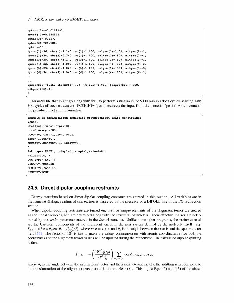
24. NMR, X-ray, and cryo-EM/ET refinement
opttet(3)=-0.0113097,
optomg(3)=0.334824,
opta1(3)=-8.657,
opta2(3)=704.786,
optkon=30,
iprot(1)=26, obs(1)=1.140, wt(1)=1.000, tolpro(1)=1.00, mltpro(1)=1,
iprot(2)=28, obs(2)=2.740, wt(2)=1.000, tolpro(2)=.500, mltpro(2)=1,
iprot(3)=30, obs(3)=1.170, wt(3)=1.000, tolpro(3)=.500, mltpro(3)=1,
iprot(4)=32, obs(4)=1.060, wt(4)=1.000, tolpro(4)=.500, mltpro(4)=3,
iprot(5)=33, obs(5)=1.060, wt(5)=1.000, tolpro(5)=.500, mltpro(5)=3,
iprot(6)=34, obs(6)=1.060, wt(6)=1.000, tolpro(6)=.500, mltpro(6)=3,
...
...
iprot(205)=1215, obs(205)=.730, wt(205)=1.000, tolpro(205)=.500,
mltpro(205)=1,
/ An mdin file that might go along with this, to perform a maximum of 5000 minimization cycles, starting with
500 cycles of steepest descent. PCSHIFT=./pcs.in redirects the input from the namelist "pcs.in" which containsthe pseudocontact shift information. Example of minimization including pseudocontact shift constraints
&cntrl
ibelly=0,imin=1,ntpr=100,
ntr=0,maxcyc=500,
ncyc=50,ntmin=1,dx0=0.0001,
drms=.1,cut=10.,
nmropt=2,pencut=0.1, ipnlty=2,
/
&wt type=’REST’, istep1=0,istep2=1,value1=0.,
value2=1.0, /
&wt type=’END’ /
DISANG=./noe.in
PCSHIFT=./pcs.in
LISTOUT=POUT 24.5. Direct dipolar coupling restraints
Energy restraints based on direct dipolar coupling constants are entered in this section. All variables are inthe namelist &align; reading of this section is triggered by the presence of a DIPOLE line in the I/O redirectionsection.
When dipolar coupling restraints are turned on, the five unique elements of the alignment tensor are treatedas additional variables, and are optimized along with the structural parameters. Their effective masses are deter-mined by the scalm parameter entered in the &cntrl namelist. Unlike some other programs, the variables usedare the Cartesian components of the alignment tensor in the axis system defined by the molecule itself: e.g.Smn ≡ 〈(3cosθm cosθn−δmn)/2〉, where m,n = x,y,z, and θx is the angle between the x axis and the spectrometerfield.[461] The factor of 105 is just to make the values commensurate with atomic coordinates, since both thecoordinates and the alignment tensor values will be updated during the refinement. The calculated dipolar splittingis then
Dcalc =−
(10−5γiγ jh
2π2r3i j
)∑
m,n=xyzcosφm ·Smn · cosφn
where φx is the angle between the internuclear vector and the x axis. Geometrically, the splitting is proportional tothe transformation of the alignment tensor onto the internuclear axis. This is just Eqs. (5) and (13) of the above
466
24.5. Direct dipolar coupling restraints
reference, with any internal motion corrections (which might be a part of Ssystem) set to unity. If there is an internalmotion correction which is the same for all observations, this can be assimilated into the alignment tensor. Thecurrent code does not allow for variable corrections for internal motion. See Ref. [462] for a fuller discussion ofthese issues.
At the end of the calculation, the alignment tensor is diagonalized to obtain information about its principalcomponents. This allows the alignment tensor to be written in terms of the "axial" and "rhombic" components thatare often used to describe alignment.
Variables in the &align namelist.
ndip Number of observed dipolar couplings to be used as restraints.
id,jd Atom numbers of the two atoms involved in the dipolar coupling.
dobsl, dobsu Limiting values for the observed dipolar splitting, in Hz. If the calculated coupling is less thandobsl, the energy penalty is proportional to (Dcalc−Dobs,l)
2; if it is larger than dobsu, the penalty isproportional to (Dcalc−Dobs,lu)
2. Calculated values between dobsl and dobsu are not penalized. Notethat dobsl must be less than dobsu; for example, if the observed coupling is -6 Hz, and a 1 Hz "buffer"is desired, you could set dobsl to -7 and dobsu to -5.
dwt The relative weight of each observed value. Default is 1.0. The penalty function is thus:
E ialign = Di
wt(Dicalc−Di
obs(u,l))2
where Dwt may vary from one observed value to the next. Note that the default value is arbitrary, anda smaller value may be required to avoid overfitting the dipolar coupling data.[462]
dataset Each dipolar peak can be associated with a "dataset", and a separate alignment tensor will be computedfor each dataset. This is generally used if there are several sets of experiments, each with a differentsample or temperature, etc., that would imply a different value for the alignment tensor. By default,there is one dataset to which each observed value is assigned.
num_datasets The number of datasets in the constraint list. Default is 1.
s11,s12,s13,s22,s23 Initial values for the Cartesian components of the alignment tensor. The tensor is traceless,so S33 is calculated as -(S11+S22). In order to have the order of magnitude of the S values be roughlycommensurate with coordinates in Angstroms, the alignment tensor values must be multiplied by 105.
gigj Product of the nuclear "g" factors for this dipolar coupling restraint. These are related to the nucleargyromagnetic rations by γN = gNβN/h. Common values are 1H = 5.5856, 13C = 1.4048, 15N = -0.5663,31P = 2.2632.
dij The internuclear distance for observed dipolar coupling. If a nonzero value is given, the distance isconsidered to be fixed at the given value. If a dij value is zero, its value is computed from the structure,and it is assumed to be a variable distance. For one-bond couplings, it is usually best to treat the bonddistance as "fixed" to an effective zero-point vibration value.[463]
dcut Controls printing of calculated and observed dipolar couplings. Only values where abs(dobs(u,l) -dcalc) is greater than dcut will be printed. Default is 0.1 Hz. Set to a negative value to print all dipolarrestraint information.
freezemol If this is set to .true., the molecular coordinates are not allowed to vary during dynamics or minimiza-tion: only the elements of the alignment tensor will change. This is useful to fit just an alignmenttensor to a given structure. Default is .false..
467

24. NMR, X-ray, and cryo-EM/ET refinement
24.6. Residual CSA or pseudo-CSA restraints
Resonance positions in partially aligned media will be shifted from their positions in isotropic media, and thiscan provide information that is very similar to residual dipolar coupling constriants. This section shows how toinput these sorts of restraints. The entry of the alignment tensor is done as in Section 24.5, so you must have aDIPOLE file (with an &align namelist) even if you don’t have any RDC restraints. Then, if there is a CSA line inI/O redirection section, that file will be read with the following inputs:
Variables in the &csa namelist.
ncsa Number of observed residual CSA peaks to be used as restraints.
icsa,jcsa,kcsa Atom numbers for the csa of interest: jcsa is the atom whose ∆σ value has been measured; icsaand kcsa are two atoms bonded to it, used to define the local axis frame for the CSA tensor. Seeamber12/test/pcsa/RST.csa for examples of how to set these.
cobsl, cobsu Limiting values for the observed residual CSA, in Hz (not ppm or ppb!). If the calculated value of ∆σ
is less than cobsl, the energy penalty is proportional to (∆σcalc−∆σobs,l)2; if it is larger than cobsu,
the penalty is proportional to (∆σcalc−∆σobs,u)2. Calculated values between cobsl and cobsu are not
penalized. Note that cobsl must be less than cobsu.
cwt The relative weight of each observed value. Default is 1.0. The penalty function is thus:
E icsa =Ci
wt(∆σ icalc−∆σ i
obs(u,l))2
where Cwt may vary from one observed value to the next. Note that the default value is arbitrary, anda smaller value may be required to avoid overfitting the data.
datasetc Each residual CSA can be associated with a "dataset", and a separate alignment tensor will be com-puted for each dataset. This is generally used if there are several sets of experiments, each with adifferent sample or temperature, etc., that would imply a different value for the alignment tensor. Bydefault, there is one dataset to which each observed value is assigned. The tensors themselves areentered for each dataset in the DIPOLE file.
field Magnetic field (in MHz) for the residual CSA being considered here. This is indexed from 1 to ncsa,and is nucleus dependent. For example, if the proton frequency is 600 MHz, then field for 13C wouldbe 150, and that for 15N would be 60.
sigma11, sigma22, sigma12, sigma13, sigma23 Values of the CSA tensor (in ppm) for atom icsa, in the localcoordinate frame defined by atoms icsa, jcsa and kcsa. See $AMBERHOME/test/pcsa/RST.csa forexamples of how to set these.
ccut Controls printing of calculated and observed residual CSAs. Only values where abs(cobs(u,l) - ccalc)is greater than ccut will be printed. Default is 0.1 Hz. Set to a negative value to print all information.
The residual CSA facility is new as of Amber 10, and has not been used as much as other partsof the NMR refinement package. You should study the example files listed above to see how thingswork. The residual CSA values should closely match those found by the RAMAH package (http://www-personal.umich.edu/~hashimi/Software.html), and testing this should be a first step in making sure you have enteredthe data correctly.
24.7. Preparing restraint files for Sander
Fig. 24.1 shows the general information flow for auxiliary programs that help prepare the restraint files. Oncethe restraint files are made, Fig. 24.2 shows a flow-chart of the general way in which sander refinements are carriedout.
468

24.7. Preparing restraint files for Sander
NOESY
peak-list
various
calibrations
7/8 column
distance
bounds
makeDIST_RST distance
restraints
makeDIST_RST volume
restraints
chemical
shift
restraints
chemical
shifts
analyze
ambiguities
MAP
file
default
MAP file
SHIFTS or
FANTASIAN
spectr um
5 column
coupling
constants
makeANG_RST J-coupling
restraints
DISANG
file
default
chirality
infor m.
makeCHIR_RST chirality
restraints
direct
dipolar
couplings
makeDIP_RST alignment
restraints
Figure 24.1.: Notation: circles represent logical information, whose format might differ from one project to thenext; solid rectangles are in a specific format (largely compatible with DIANA and other programs),and are intended to be read and edited by the user; ellipses are specific to sander, and are generallynot intended to be read or edited manually. The conversion of NOESY volumes to distance boundscan be carried out by a variety of programs such as mardigras or xpk2bound that are not includedwith Amber. Similarly, the analysis and partial assignment of ambiguous or overlapped peaks is aseparate task; at TSRI, these are typically carried out using the programs xpkasgn and filter.pl
469

24. NMR, X-ray, and cryo-EM/ET refinement
gener ic
PDB-file
protonate Amber
PDB-file
LEaPpr mtop &
pr mcrd
files
sander
control
file
SANDERNMR
restraints
sander
output
sviolviolation
statistics
Amber
coordinates
ambpdb output
pdb-files
Figure 24.2.: General organization of NMR refinement calculations.
The basic ideas of this scheme owe a lot to the general experience of the NMR community over the pastdecade. Several papers outline procedures in the Scripps group, from which a lot of the NMR parts of sanderare derived.[454, 464–468] They are by no means the only way to proceed. We hope that the flexibility incorpo-rated into sander will encourage folks to experiment with refinement protocols.
24.7.1. Preparing distance restraints: makeDIST_RST
The makeDIST_RST program converts a simplified description of distance bounds into a detailed input forsander. A variety of input and output filenames may be specified on the command line:
input:
-upb <filename> 7-col file of upper distance bounds, OR
-ual <filename> 8-col file of upper and lower bounds, OR
-vol <filename> 7-col file of NOESY volumes
-pdb <filename> Brookhaven format file
-map <filename> MAP file (default:map.DG-AMBER)
-les <filename> LES atom mappings, made by addles
output:
-dgm <filename> DGEOM95 restraint format
-rst <filename> SANDER restraint format
-svf <filename> Sander Volume Format, for NOESY refinement
other options:
-help (gives you this explanation, overrides other parameters)
-report (gives you short runtime diagnostic output)
-nocorr (do not correct upper bound for r**-6 averaging)
-altdis (use alternative form for the distance restraints)
The 7/8 column distance bound file is essentially that used by the DIANA or DISGEO programs. It consists ofone-line per restraint, which would typically look like the following:
470

24.7. Preparing restraint files for Sander
23 ALA HA 52 VAL H 3.8 # comments go here
The first three columns identify the first proton, the next three the second proton, and the seventh column gives theupper bound. Only the first three letters of the residue name are used, so that DIANA files that contain residueslike "ASP-" will be correctly interpreted. An alternate, 8-column, format has both upper and lower bounds as theseventh and eighth columns, respectively. A typical line might in an "8-col" file might look like this:
23 ALA HA 52 VAL H 3.2 3.8 # comments go here
Here the lower bound is 3.2 Åand the upper bound is 3.8 Å. Comments typically identify the spectrum and peak-number or other identification that allow cross-referencing back to the appropriate spectrum. If the commentcontains the pattern "<integer>:<integer>", then the first integer is treated as a peak-identifier, and the second asa spectrum-identifier. These identifiers go into the ixpk and nxpk variables, and will later be printed out in sander,to facilitate going back to the original spectra to track down violations, etc.
The format for the -vol option is the same as for the -upb option except that the seventh column holds a peakintensity (volume) value, rather than a distance upper bound.
The input PDB file must exactly match the Amber prmtop file that will be used; use the ambpdb -aatm commandto create this.
If all peaks involved just single protons, and were fully assigned, this is all that one would need. In general,though, some peaks (especially methyl groups or fast-rotating aromatic rings) represent contributions from morethan one proton, and many other peaks may not be fully assigned. Sander handles both of these situations in thesame way, through the notion of an "ambiguous" peak, that may correspond to several assignments. These peaksare given two types of special names in the 7/8-column format file:
1. Commonly-occurring ambiguities, like the lack of stereospecific assignments to two methylene protons, aregiven names defined in the default MAP file. These names, also more-or-less consistent with DIANA, arelike the names of "pseudo-atoms" that have long been used to identify such partially assigned peaks, e.g."QB" refers to the (HB2,HB3) combination in most residues, and "MG1" in valine refers collectively to thethree methyl protons at position CG1, etc.
2. There are generally also molecule-specific ambiguities, arising from potential overlap in a NOESY spectrum.Here, the user assigns a unique name to each such ambiguity or overlap, and prepares a list of the potentialassignments. The names are arbitrary, but might be constructed, for example, from the chemical shifts thatidentify the peak, e.g. "p_2.52" might identify the set of protons that could contribute to a peak at 2.52 ppm.The chemical shift list can be used to prepare a list of potential assignments, and these lists can often bepruned by comparison to approximate or initial structures.
The default and molecule-specific MAP files are combined into a single file, which is used, along with the7-column restraint file, the the program makeDIST_RST to construct the actual sander input files. You shouldconsult the help file for makeDIST_RST for more information. For example, here are some lines added to theMAP file for a recent TSRI refinement:
AMBIG n2:68 = HE 86 HZ 86
AMBIG n2:72 = HE 24 HD 24 HZ 24
AMBIG n2:73 = HN 81 HZ 13 HE 13 HD 13 HZ 24
AMBIG n2:78 = HN 76 HZ 13 HE 13 HZ 24
AMBIG n2:83 = HN 96 HN 97 HD 97 HD 91
AMBIG n2:86 = HD1 66 HZ2 66
AMBIG n2:87 = HN 71 HH2 66 HZ3 66 HD1 66
Here the spectrum name and peak number were used to construct a label for each ambiguous peak. Then, an entryin the restraint file might look like this:
123 GLY HN 0 AMB n2:68 5.5
indicating a 5.5 Åupper bound between the amide proton of Gly 123 and a second proton, which might be eitherthe HE or HZ protons of residue 86. (The "zero" residue number just serves as a placeholder, so that there will be
471
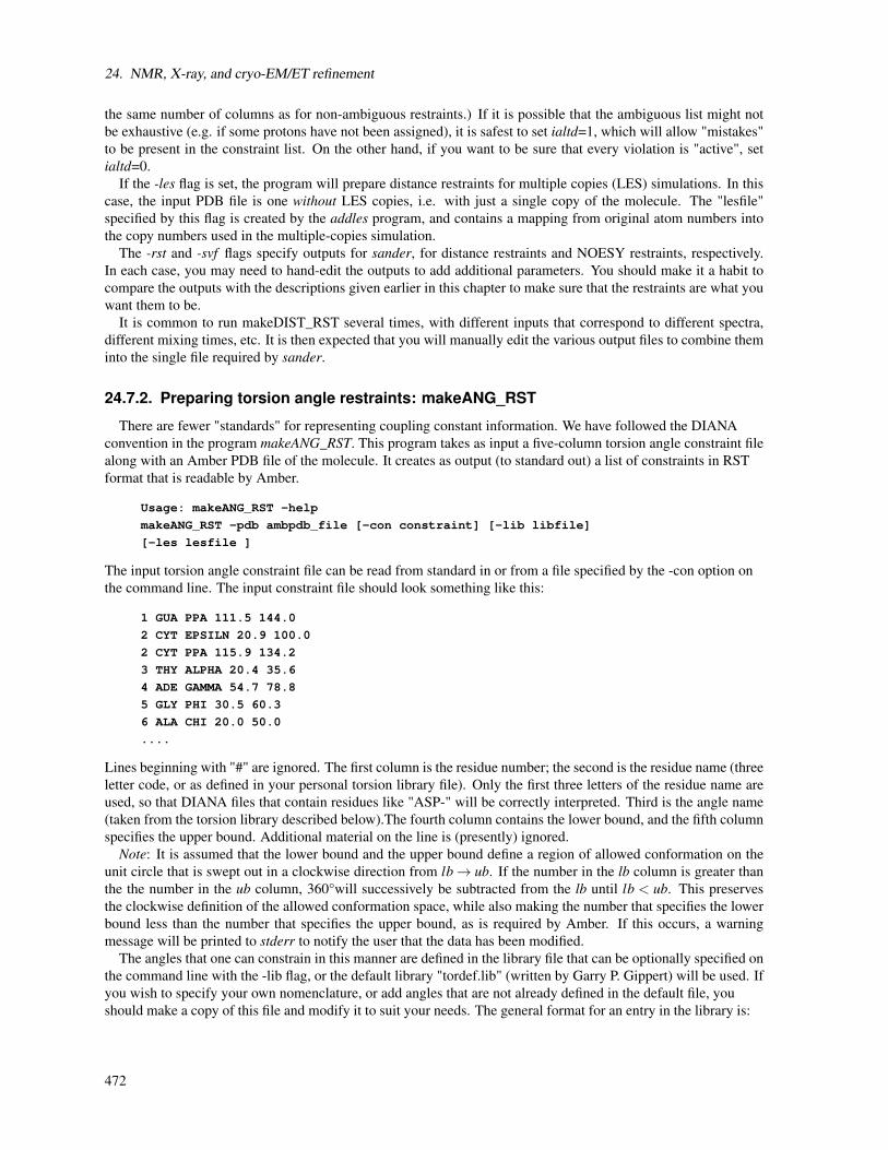
24. NMR, X-ray, and cryo-EM/ET refinement
the same number of columns as for non-ambiguous restraints.) If it is possible that the ambiguous list might notbe exhaustive (e.g. if some protons have not been assigned), it is safest to set ialtd=1, which will allow "mistakes"to be present in the constraint list. On the other hand, if you want to be sure that every violation is "active", setialtd=0.
If the -les flag is set, the program will prepare distance restraints for multiple copies (LES) simulations. In thiscase, the input PDB file is one without LES copies, i.e. with just a single copy of the molecule. The "lesfile"specified by this flag is created by the addles program, and contains a mapping from original atom numbers intothe copy numbers used in the multiple-copies simulation.
The -rst and -svf flags specify outputs for sander, for distance restraints and NOESY restraints, respectively.In each case, you may need to hand-edit the outputs to add additional parameters. You should make it a habit tocompare the outputs with the descriptions given earlier in this chapter to make sure that the restraints are what youwant them to be.
It is common to run makeDIST_RST several times, with different inputs that correspond to different spectra,different mixing times, etc. It is then expected that you will manually edit the various output files to combine theminto the single file required by sander.
24.7.2. Preparing torsion angle restraints: makeANG_RST
There are fewer "standards" for representing coupling constant information. We have followed the DIANAconvention in the program makeANG_RST. This program takes as input a five-column torsion angle constraint filealong with an Amber PDB file of the molecule. It creates as output (to standard out) a list of constraints in RSTformat that is readable by Amber.
Usage: makeANG_RST -help
makeANG_RST -pdb ambpdb_file [-con constraint] [-lib libfile]
[-les lesfile ]
The input torsion angle constraint file can be read from standard in or from a file specified by the -con option onthe command line. The input constraint file should look something like this:
1 GUA PPA 111.5 144.0
2 CYT EPSILN 20.9 100.0
2 CYT PPA 115.9 134.2
3 THY ALPHA 20.4 35.6
4 ADE GAMMA 54.7 78.8
5 GLY PHI 30.5 60.3
6 ALA CHI 20.0 50.0
....
Lines beginning with "#" are ignored. The first column is the residue number; the second is the residue name (threeletter code, or as defined in your personal torsion library file). Only the first three letters of the residue name areused, so that DIANA files that contain residues like "ASP-" will be correctly interpreted. Third is the angle name(taken from the torsion library described below).The fourth column contains the lower bound, and the fifth columnspecifies the upper bound. Additional material on the line is (presently) ignored.
Note: It is assumed that the lower bound and the upper bound define a region of allowed conformation on theunit circle that is swept out in a clockwise direction from lb→ ub. If the number in the lb column is greater thanthe the number in the ub column, 360°will successively be subtracted from the lb until lb < ub. This preservesthe clockwise definition of the allowed conformation space, while also making the number that specifies the lowerbound less than the number that specifies the upper bound, as is required by Amber. If this occurs, a warningmessage will be printed to stderr to notify the user that the data has been modified.
The angles that one can constrain in this manner are defined in the library file that can be optionally specified onthe command line with the -lib flag, or the default library "tordef.lib" (written by Garry P. Gippert) will be used. Ifyou wish to specify your own nomenclature, or add angles that are not already defined in the default file, youshould make a copy of this file and modify it to suit your needs. The general format for an entry in the library is:
472

24.7. Preparing restraint files for Sander
LEU PSI N CA C N+
where the first column is the residue name, the second column is the angle name that will appear in the input filewhen specifying this angle, and the last four columns are the atom names that define the torsion angle. When atorsion angle contains atom(s) from a preceding or succeeding residue in the structure, a "-" or "+" is appendedto those atom names in the library, thereby specifying that this is the case. In the example above, the atoms thatdefine PSI for LEU residues are the N, CA, and C atoms of that same LEU and the N atom of the residue after thatLEU in the primary structure. Note that the order of atoms in the definition is important and should reflect that thetorsion angle rotates about the two central atoms as well as the fact that the four atoms are bonded in the order thatis specified in the definition.
If the first letter of the second field is "J", this torsion is assumed to be a J-coupling constraint. In that case,three additional floats are read at the end of the line, giving the A,B and C coefficients for the Karplus relation forthis torsion. For example:
ALA JHNA H N CA HA 9.5 -1.4 0.3
will set up a J-coupling restraint for the HN-HA 3-bond coupling, assuming a Karplus relation with A,B, C as 9.5,-1.4 and 0.3. (These particular values are from Brüschweiler and Case, JACS 116: 11199 (1994).)
This program also supports pseudorotation phase angle constraints for prolines and nucleic acid sugars; each ofthese will generate restraints for the 5 component angles which correspond to the lb and ub values of the inputpseudorotation constraint. In the torsion library, a pseudorotation definition looks like:
PSEUDO CYT PPA NU0 NU1 NU2 NU3 NU4
CYT NU0 C4’ O4’ C1’ C2’
CYT NU1 O4’ C1’ C2’ C3’
CYT NU2 C1’ C2’ C3’ C4’
CYT NU3 C2’ C3’ C4’ O4’
CYT NU4 C3’ C4’ O4’ C1’
The first line describes that a PSEUDOrotation angle is to be defined for CYT that is called PPA and is made up ofthe five angles NU0-NU4. Then the definition for NU0-NU4 should also appear in the file in the same format asthe example given above for LEU PSI.
PPA stands for Pseudorotation Phase Angle and is the angle that should appear in the input constraint file whenusing pseudorotation constraints. The program then uses the definition of that PPA angle in the library file to lookfor the 5 other angles (NU0-NU4 in this case) which it then generates restraints for. PPA for proline residues isincluded in the standard library as well as for the DNA nucleotides.
If the -les flag is set, the program will prepare torsion angle restraints for multiple copies (LES) simulations. Inthis case, the input PDB file is one without LES copies, i.e. with just a single copy of the molecule. The "lesfile"specified by this flag is created by the addles program, and contains a mapping from original atom numbers intothe copy numbers used in the multiple-copies simulation.
Torsion angle constraints defined here cannot span two different copy sets, i.e., there cannot be some atoms ofa particular torsion that are in one multiple copy set, and other atoms from the same torsion that are in other copysets. It is OK to have some atoms with single copies, and others with multiple copies in the same torsion. Theprogram will create as many duplicate torsions as there are copies.
A good alternative to interpreting J-coupling constants in terms of torsion angle restraints is to refine directlyagainst the coupling constants themselves, using an appropriate Karplus relation. See the discussion of the variableRJCOEF, above.
24.7.3. Chirality restraints: makeCHIR_RST
Usage: makeCHIR_RST <pdb-file> <output-constraint-file>
We also find it useful to add chirality constraints and trans-peptide ω constraints (where appropriate) to preventchirality inversions or peptide bond flips during the high-temperature portions of simulated annealing runs. Theprogram makeCHIR_RST will create these constraints. Note that you may have to edit the output of this programto change trans peptide constraints to cis, as appropriate.
473

24. NMR, X-ray, and cryo-EM/ET refinement
24.7.4. Direct dipolar coupling restraints: makeDIP_RST
For simulations with residual dipolar coupling restraints, the makeDIP_RST.protein, makeDIP_RST.dna andmakeDIP_RST.diana are simple codes to prepare the input file. Use -help to obtain a more detailed description ofthe usage. For now, this code only handles backbone NH and CαH data. The header specifying values for variousparameters needs to be manually added to the output of makeDIP_RST.
Use of residual dipolar coupling restraints is new both for Amber and for the general NMR community. Re-finement against these data should be carried out with care, and the optimal values for the force constant, penaltyfunction, and initial guesses for the alignment tensor components are still under investigation. Here are somesuggestions from the experiences so far:
1. Beware of overfitting the dipolar coupling data in the expense of Amber force field energy. These dipolarcoupling data are very sensitive to tiny changes in the structure. It is often possible to drastically improvethe fitting by making small distortions in the backbone angles. We recommend inclusion of explicit anglerestraints to enforce ideal backbone geometry, especially for those residues that have corresponding residualdipolar coupling data.
2. The initial values for the Cartesian components of the alignment tensor can influence the final structure andalignment if the structure is not fixed (ibelly = 0). For a fixed structure (ibelly = 1), these values do notmatter. Therefore, the current "best" strategy is to fit the experimental data to the fixed starting structure, anduse the alignment tensor[s] obtained from this fitting as the initial guesses for further refinement.
3. Amber is capable of simultaneously fitting more than one set of alignment data. This allows the use ofindividually obtained datasets with different alignment tensors. However, if the different sets of data haveequal directions of alignment but different magnitudes, using an overall scaling factor for these data with asingle alignment tensor could greatly reduce the number of fitting parameters.
4. Because the dipolar coupling splittings depend on the square root of the order parameters (0≤ S2≤1), theseorder parameters describing internal motion of individual residues are often neglected (N. Tjandra and A.Bax, Science 278, 1111-1113, 1997). However, the square root of a small number can still be noticeablysmaller than 1, so this may introduce undesirable errors in the calculations.
24.7.5. Using NMR exchange format (NEF) files
The NMR community, in collaboration with the worldwide PDB, is developing a common format for encodingof NMR restraints, including all of the kinds discussed above. This format is not yet finalized, but we areincluding here a conversion script, nef_to_RST, that would convert these files to sander format. Because thisformat is so new, and is still subject to revisions, care should be taken in using this script: make sure that theoutput files do what they should be doing. Here are the usage instructions (which you can also get by typing“nef_to_RST -help” at the command line:
# nef_to_RST
convert NEF restraints to Amber format
input:
-nef <filename>: NEF file
-pdb <filename>: PDBFILE using AMBER nomenclature and numbering
-map <filename>: MAP file (default:map.NEF-AMBER)
output:
-rst <filename>: SANDER restraint format
-rdc <filename>: SANDER DIP format
other options:
-nocorr (do not correct upper bound for r**-6 averaging)
-altdis (use alternative form for the distance restraints)
-help (gives you this explanation, overrides other parameters)
474

24.8. Getting summaries of NMR violations
-report (gives you short runtime diagnostic output)
errors come to stderr.
24.7.6. fantasian
A program to evaluate magnetic anisotropy tensor parameters
Ivano Bertini
Depart. of Chemistry, Univ. of Florence, Florence, Italy
e-mail: [email protected]
INPUT FILES:
Observed shifts file (pcshifts.in):
1st column --> residue number
2nd column --> residue name
3rd column --> proton name
4th column --> observed pseudocontact shift value
5th column --> multiplicity of the NMR signal (for example it is 3 for of a methyl group)
6th column --> relative tolerance
7th column --> relative weight
Amber pdb file (parm.pdb): coordinates file in PDB format. If you need to use a solution NMR family of structuresyou have to superimpose the structures before to use them.
OUTPUT FILES:
Observed out file (obs.out): This file is built and read by the program itself, it reports the data read from the inputfiles.
output file (res.out): The main output file. In this file the result of the fitting is reported. Using fantasian itis possible to define an internal reference system to visualize the orientation of the tensor axes. Then in this fileyou can find PDB format lines (ATOM) which can be included in a PDB file to visualize the internal referencesystem and the tensor axes. In the main output file all the three equivalent permutations of the tensor parameterswith respect to the reference system are reported. The summary of the minimum and maximum errors and that ofsquared errors are also reported.
Example files: in the directory example there are all the files necessary to run a fantasian calculation:
fantasian.com --> run file
pcshifts.in --> observed shifts file
parm.pdb --> coordinate file in PDB format
obs.out --> data read from input files
res.out --> main output file ~
24.8. Getting summaries of NMR violations
If you specify LISTOUT=POUT when running sander, the output file will contain a lot of detailed informationabout the remaining restraint violations at the end of the run. When running a family of structures, it can be usefulto process these output files with sviol, which takes a list of sander output files on the command line, and sends asummary of energies and violations to STDOUT. If you have more than 20 or so structures to analyze, the outputfrom sviol becomes unwieldy. In this case you may also wish to use sviol2, which prints out somewhat less detailedinformation, but which can be used on larger families of structures. The senergy script gives a more detailed viewof force-field energies from a series of structures. (We thank the TSRI NMR community for helping to put thesescripts together, and for providing many useful suggestions.)
475

24. NMR, X-ray, and cryo-EM/ET refinement
24.9. Time-averaged restraints
The model of the previous sections involves the "single-average-structure" idea, and tries to fit all constraints toa single model, with minimal deviations. A generalization of this model treats distance constraints arising fromfrom NOE crosspeaks (for example) as being the average distance determined from a trajectory, rather than as thesingle distance derived from an average structure.
Time-averaged bonds and angles are calculated as
r = (1/C)
∫ t
0e(t′−t)/τ r(t ′)−idt ′
−1/i
(24.1)
where
r = time-averaged value of the internal coordinate (distance or angle)
t = the current time
τ = the exponential decay constant
r(t ′) = the value of the internal coordinate at time t’
i = average is over internals to the inverse of i. Usually i = 3 or 6 for NOE distances, and -1 (linearaveraging) for angles and torsions.
C = a normalization integral.
Time-averaged torsions are calculated as
< ϕ >= tan−1 (< sin(φ)> / < cos(φ)>)
where φ is the torsion, and < sin(φ)> and < cos(φ)> are calculated using the equation above with sin(φ(t ′))or cos(φ(t ′)) substituted for r(t ′).
Forces for time-averaged restraints can be calculated either of two ways. This option is chosen with the DISAVI/ ANGAVI / TORAVI commands. In the first (the default),
∂E/∂x = (∂E/∂ r)(∂ r/∂ r(t))(∂ r(t)/∂x) (24.2)
(and analogously for y and z). The forces then correspond to the standard flat-bottomed well functional form, withthe instantaneous value of the internal replaced by the time-averaged value. For example, when r3 < r < r4,
E = k3(r− r3)2
and similarly for other ranges of r.When the second option for calculating forces is chosen (IINC = 1 on a DISAVI, ANGAVI or TORAVI card),
forces are calculated as
∂E/∂x = (∂E/∂ r)(∂ r(t)/∂x) (24.3)
For example, when r3 < r < r4,
∂E/∂x = 2k3(r− r3)(∂ r(t)/∂x)
Integration of this equation does not give Eq. 24.2, but rather a non-intuitive expression for the energy (althoughone that still forces the bond to the target range). The reason that it may sometimes be preferable to use this secondoption is that the term ∂ r/∂ r(t), which occurs in the exact expression [Eq. 24.2], varies as (r/r(t))1+i. Wheni=3, this means the forces can be varying with the fourth power the distance, which can possibly lead to very largetransient forces and instabilities in the molecular dynamics trajectory. [Note that this will not be the case whenlinear scaling is performed, i.e. when i = −1, as is generally the case for valence and torsion angles. Thus, forlinear scaling, the default (exact) force calculation should be used].
476

24.10. Multiple copies refinement using LES
It should be noted that forces calculated using Eq. 24.3 are not conservative forces, and would cause the systemto gradually heat up, if no velocity rescaling were performed. The temperature coupling algorithm should act tomaintain the average temperature near the target value. At any rate, this heating tendency should not be a problemin simulations, such as fitting NMR data, where MD is being used to sample conformational space rather than toextract thermodynamic data.
This section has described the methods of time-averaged restraints. For more discussion, the interested user isurged to consult studies where this method has been used.[469–473]
24.10. Multiple copies refinement using LES
NMR restraints can be made compatible with the multiple copies (LES) facility; see the following chapter formore information about LES. To use NMR constraints with LES, you need to do two things:
(1) Add a line like "file wnmr name=(lesnmr) wovr" to your input to addles. The filename (lesnmr in thisexample) may be whatever you wish. This will cause addles to output an additional file that is needed at the nextstep.
(2) Add "-les lesnmr" to the command line arguments to makeDIST_RST. This will read in the file createdby addles containing information about the copies. All NMR restraints will then be interpreted as "ambiguous"restraints, so that if any of the copies satisfies the restraint, the penalty goes to zero.
Note that although this scheme has worked well on small peptide test cases, we have yet not used it extensivelyfor larger problems. This should be treated as an experimental option, and users should use caution in applying orinterpreting the results.
24.11. Some sample input files
The next few pages contain excerpts from some sample NMR refinement files used at TSRI. The first examplejust sets up a simple (but often effective) simulated annealing run. You may have to adjust the length, temperaturemaximum, etc. somewhat to fit your problem, but these values work well for many "ordinary" NMR problems.
24.11.1. 1. Simulated annealing NMR refinement
15ps simulated annealing protocol
&cntrl
nstlim=15000, ntt=1, (time limit, temp. control)
ntpr=500, pencut=0.1, (control of printout)
ipnlty=1, nmropt=1, (NMR penalty function options)
vlimit=10, (prevent bad temp. jumps)
ntb=0, (non-periodic simulation)
/
&ewald
eedmeth=5, (use r dielectric)
/
#
# Simple simulated annealing algorithm:
#
# from steps 0 to 1000: raise target temperature 10->1200K
# from steps 1000 to 3000: leave at 1200K
# from steps 3000 to 15000: re-cool to low temperatures
#
&wt type=’TEMP0’, istep1=0,istep2=1000,value1=10.,
value2=1200., /
&wt type=’TEMP0’, istep1=1001, istep2=3000, value1=1200.,
477

24. NMR, X-ray, and cryo-EM/ET refinement
value2=1200.0, /
&wt type=’TEMP0’, istep1=3001, istep2=15000, value1=0.,
value2=0.0, /
#
# Strength of temperature coupling:
# steps 0 to 3000: tight coupling for heating and equilibration
# steps 3000 to 11000: slow cooling phase
# steps 11000 to 13000: somewhat faster cooling
# steps 13000 to 15000: fast cooling, like a minimization
#
&wt type=’TAUTP’, istep1=0,istep2=3000,value1=0.2,
value2=0.2, /
&wt type=’TAUTP’, istep1=3001,istep2=11000,value1=4.0,
value2=2.0, /
&wt type=’TAUTP’, istep1=11001,istep2=13000,value1=1.0,
value2=1.0, /
&wt type=’TAUTP’, istep1=13001,istep2=14000,value1=0.5,
value2=0.5, /
&wt type=’TAUTP’, istep1=14001,istep2=15000,value1=0.05,
value2=0.05, /
#
# "Ramp up" the restraints over the first 3000 steps:
#
&wt type=’REST’, istep1=0,istep2=3000,value1=0.1,
value2=1.0, /
&wt type=’REST’, istep1=3001,istep2=15000,value1=1.0,
value2=1.0, /
&wt type=’END’ /
LISTOUT=POUT (get restraint violation list)
DISANG=RST.f (file containing NMR restraints)
The next example just shows some parts of the actual RST file that sander would read. This file would ordinarilynot be made or edited by hand; rather, run the programs makeDIST_RST, makeANG_RST and makeCHIR_RST,combining the three outputs together to construct the RST file.
24.11.2. Part of the RST.f file referred to above
# first, some distance constraints prepared by makeDIST_RST:
# (comment line is input to makeRST, &rst namelist is output)
#
#( proton 1 proton 2 upper bound)
#---------------------------------------------
#
# 2 ILE HA 3 ALA HN 4.00
#
&rst iat= 23, 40, r3= 4.00, r4= 4.50,
r1 = 1.3, r2 = 1.8, rk2=0.0, rk3=32.0, ir6=1, /
#
# 3 ALA HA 4 GLU HN 4.00
#
&rst iat= 42, 50, r3= 4.00, r4= 4.50, /
#
# 3 ALA HN 3 ALA MB 5.50
478

24.11. Some sample input files
#
&rst iat= 40, -1, r3= 6.22, r4= 6.72,
igr1= 0, 0, 0, 0, igr2= 44, 45, 46, 0, /
#
# .......etc......
#
# next, some dihedral angle constraints, from makeANG_RST:
#
&rst iat= 213, 215, 217, 233, r1=-190.0,
r2=-160.0, r3= -80.0, r4= -50.0, /
&rst iat= 233, 235, 237, 249, r1=-190.0,
r2=-160.0, r3= -80.0, r4= -50.0, /
# .......etc.......
#
# next, chirality and omega constraints prepared by makeCHIR_RST:
#
#
# chirality for residue 1 atoms: CA CG HB2 HB3
&rst iat= 3 , 8 , 6 , 7 ,
r1=10., r2=60., r3=80., r4=130., rk2 = 10., rk3=10., /
#
# chirality for residue 1 atoms: CB SD HG2 HG3
&rst iat= 5 , 11 , 9 , 10 , /
#
# chirality for residue 1 atoms: N C HA CB
&rst iat= 1 , 18 , 4 , 5 , /
#
# chirality for residue 2 atoms: CA CG2 CG1 HB
&rst iat= 22 , 26 , 30 , 25 , /
#
......etc........
# trans-omega constraint for residue 2
&rst iat= 22 , 20 , 18 , 3 ,
r1=155., r2=175., r3=185., r4=205., rk2 = 80., rk3=80., /
#
# trans-omega constraint for residue 3
&rst iat= 41 , 39 , 37 , 22 , /
#
# trans-omega constraint for residue 4
&rst iat= 51 , 49 , 47 , 41 , /
#
# ......etc........
#
The next example is an input file for volume-based NOE refinement. As with the distance/angle RST file shown above, the user would generally not construct this file, but create it from a "7-column" file using the makeDIST_RST program. Hand-editing might be used at the top of the file, to change the correlation times, etc.
24.11.3. 3. Sample NOESY intensity input file
# A part of a NOESY intensity file:
&noeexp
id2o=1, (exchangeable protons removed)
oscale=6.21e-4, (scale between exp. and calc. intensity units)
taumet=0.04, (correlation time for methyl rotation, in ns.)
taurot=4.2, (protein tumbling time, in ns.)
479

24. NMR, X-ray, and cryo-EM/ET refinement
NPEAK = 13*3, (three peaks, each with 13 mixing times)
EMIX = 2.0E-02, 3.0E-02, 4.0E-02, 5.0E-02, 6.0E-02,
8.0E-02, 0.1, 0.126, 0.175, 0.2, 0.25, 0.3, 0.35,
(mixing times, in sec.)
IHP(1,1) = 13*423, IHP(1,2) = 13*1029, IHP(1,3) = 13*421,
(number of the first proton)
JHP(1,1) = 78*568, JHP(1,2) = 65*1057, JHP(1,3) = 13*421,
(number of the second proton)
AEXP(1,1) = 5.7244, 7.6276, 7.7677, 9.3519,
10.733, 15.348, 18.601,
21.314, 26.999, 30.579,
33.57, 37.23, 40.011,
(intensities for the first cross-peak)
AEXP(1,2) = 8.067, 11.095, 13.127, 18.316,
22.19, 26.514, 30.748,
39.438, 44.065, 47.336,
54.467, 56.06, 60.113,
AEXP(1,3) = 7.708, 13.019, 15.943, 19.374,
25.322, 28.118, 35.118,
40.581, 49.054, 53.083,
56.297, 59.326, 62.174,
/
SUBMOL1
RES 27 27 29 29 39 41 57 57 70 70 72 72 82 82 (residues in this submol)
END END
Next, we illustrate the form of the file that holds residual dipolar coupling restraints. Again, this would generallybe created from a human-readable input using the program makeDIP_RST.
24.11.4. Residual dipolar restraints, prepared by makeDIP_RST:
&align
ndip=91, dcut=-1.0, gigj = 37*-3.1631, 54*7.8467,
s11=3.883, s22=53.922, s12=33.855, s13=-4.508, s23=-0.559,
id(1)=188, jd(1)=189, dobsu(1)= 6.24, dobsl(1)= 6.24,
id(2)=208, jd(2)=209, dobsu(2)= -10.39, dobsl(1)= -10.39,
id(3)=243, jd(3)=244, dobsu(3)= -8.12, dobsl(1)= -8.12,
....
id(91)=1393, jd(91)=1394, dobsu(91)= -19.64, dobsl(91) = -19.64,
/
Finally, we show how the detailed input to sander could be used to generate a more complicated restraint. Here iswhere the user would have to understand the details of the RST file, since there are no "canned" programs to createthis sort of restraint. This illustrates, though, the potential power of the program.
24.11.5. A more complicated constraint
# 1) Define two centers of mass. COM1 is defined by
# C1 in residue 1; C1 in residue 2; N2 in residue 3; C1 in residue 4.
# COM2 is defined by C4 in residue 1; O4 in residue 1; N* in residue 1.
# (These definitions are effected by the igr1/igr2 and grnam1/grnam2
# variables; You can use up to 200 atoms to define a center-of-mass
# group)
480
24.12. X-ray Crystallography Refinement using SANDER
#
# 2) Set up a distance restraint between COM1 and COM2 which goes from a
# target value of 5.0A to 2.5A, with a force constant of 1.0, over steps 1-5000.
#
# 3) Set up a distance restraint between COM1 and COM2 which remains fixed
# at the value of 2.5A as the force slowly constant decreases from
# 1.0 to 0.01 over steps 5001-10000.
#
# 4) Sets up no distance restraint past step 10000, so that free (unrestrained)
# dynamics takes place past this step.
#
&rst iat=-1,-1, nstep1=1,nstep2=5000,
iresid=1,irstyp=0,ifvari=1,ninc=0,imult=0,ir6=0,ifntyp=0,
r1=0.00000E+00,r2=5.0000,r3=5.0000, r4=99.000,rk2=1.0000,rk3=1.0000,
r1a=0.00000E+00,r2a=2.5000,r3a=2.5000, r4a=99.000,rk2a=1.0000,rk3a=1.0000,
igr1 = 2,3,4,5,0, grnam1(1)=’C1’,grnam1(2)=’C1’,grnam1(3)=’N2’,
grnam1(4)=’C1’, igr2 = 1,1,1,0, grnam2(1)=’C4’,grnam2(2)=’O4’,grnam2(3)=’N*’,
/
&rst iat=-1,-1, nstep1=5001,nstep2=10000,
iresid=1,irstyp=0,ifvari=1,ninc=0,imult=0,ir6=0,ifntyp=0,
r1=0.00000E+00,r2=2.5000,r3=2.5000, r4=99.000,rk2=1.0000,rk3=1.0000,
r1a=0.00000E+00,r2a=2.5000,r3a=2.5000, r4a=99.000,rk2a=1.0000,rk3a=0.0100,
igr1 = 2,3,4,5,0, grnam1(1)=’C1’,grnam1(2)=’C1’,grnam1(3)=’N2’,
grnam1(4)=’C1’, igr2 = 1,1,1,0, grnam2(1)=’C4’,grnam2(2)=’O4’,grnam2(3)=’N*’,
/
24.12. X-ray Crystallography Refinement using SANDER
An interface program links the SANDER and Crystallography and NMR System (CNS) software packages[474]to run QM/MM refinement on X-ray crystal structures, which in many instances will lead to an improvement ofX-ray crystal structure quality for medium to low resolution datasets.[475, 476] The QM calculation is enabledby a linear scaling semi-empirical technique, the divide-and-conquer method, allowing large portions of a proteinto be studied at a quantum mechanical level of theory while still retaining charge effects from the surroundingprotein.[301, 302, 477]
SANDER computes forces to make an additional call to the interface program, where the atomic coordinates areoutput to a scratch file, CNS is then invoked via a system call to calculate the X-ray target function and its gradientin Cartesian space based on the coordinates in the scratch file. In practice, this is accomplished by modifyingthe CNS input script, minimize.inp. It does not perform minimization but only evaluates and outputs the X-raytarget function and gradient based on the input structure. Next the X-ray target function and the gradient depositedin the scratch files are read into SANDER and added to the physical energy and gradient according to followingequations. The QM/MM refinement proceeds by minimizing the total target function.
Etotal = Echem +wxrayExray
The QM/MM setup in SANDER is discussed in Chapter 10. In order to run QM/MM refinement in Amber, youshould have CNS already installed and set up the environment variables for CNS in your shell script. Make sureyou can run “cns_solve < minimize.inp > minimize.out” directly from your working directory. Convertthe PDB structure factors file into CNS format. Generate the input topology and coordinate files for the CNSrefinement. If necessary, construct topology and parameter files for unusual ligands as well. The initial coordinatesin the SANDER and CNS input files should be consistent with one another. Provide the necessary (and correct) in-formation about crystal structure in the minimize.inp, such as crystal data, space group, etc. Change the weightingfactor (wxray) to balance QM/MM chemical data and the crystallographic data as appropriate.
File Usage
481

24. NMR, X-ray, and cryo-EM/ET refinement
sander [-help] [-O] -i qmmmin -o qmmmout -p prmtop -c inpcrd -x qmmmcrd -cns
Files for sanderqmmmin Control data for the QM/MM minimization runprmtop Molecular topology, force field, periodic box type, atom and residue namesinprcd Initial coordinates
Files for CNSminimize.inp Modified minimization inputprotein.cv Structure factors file in cns formatxref.in Link file connected between sander and CNSgenerate.mtf Topology file in CNS formatgenerate.pdb Initial coordinates in CNS format
Sample inputs and outputs are in the $AMBERHOME/test/1vrp_xray directory.
24.13. EMAP restraints for rigid and flexible fitting into EM maps
EMAP restrained simulation[350, 478] was developed to incorporate electron microscopy (EM) image infor-mation into macromolecular structure determination. Different from NMR and X-ray data, EM images have lowresolutions (5~50Å). However, EM images of large molecular assemblies up to millions of atoms and in variousbiologically relevant environments are available. These low resolution images provide precious structural infor-mation that can help to determine structures of many molecular assemblies and machineries[478–488].
With EMAP restraints, Sander and PMEMD can be used to perform both rigid[478] and flexible[350] fittingof molecules into experimental maps of complexes to obtain both complex structures and conformations agreeingwith experimental maps. In addition to experimental map information, homologous structural information can beused by EMAP to perform targeted conformational search (TCS) to induce simulation systems to form structuresof interest.
If the restraint map or structure is very different from the starting conformation, SGLD is recommended toinduce large conformational change by setting isgld=1. This is often used to simulate conformational transitionbetween different states. See the Sampling and free energy search section 21.1 for details on running SGLD.
If domain motion is desired while domain structures need to be maintained, one can use an EMAP restraintgenerated from the initial coordinates for each domain and set move=1 to allow the restraint map to move with thedomain, so that domains can search the conformational space without unfolding or changing shape.
Each EMAP restraint is defined by a map file and a selection of atoms, as well as related parameters. MultipleEMAP restraints can be defined. The map can be either input from an image file, or generated from a pdb structureor derived from the starting coordinates. The definition of EMAP restraints are read in from the input file as“&emap” namelists. The following are variables in each &emap namelist.
mapfile The filename of a restraint map or structure. The restraint maps must be in “map”, “ccp4”, or “mrc”format. The structure must be in pdb format. The structure need not be the same as the simulationsystem. A resolution can be specified for the conversion to a density map. When a blank filenameis specified, mapfile=”, the input coordinates of the masked atoms will be used to generate a restraintmap (default=”).
atmask The atom mask for selecting atoms to be restrained (default=’:*’).
fcons The restraining constant (default=0.05 kcal/g).
move Allow the restraint map to move when move>0 (default=0).
resolution The resolution used to convert an atomic structure to a map (default=2 Å).
ifit Perform rigid fitting before simulation when ifit>0. One would do this when the initial coordinatesdon’t match those of the map (default=0). When ifit=1, the map is transformed (by translation and
482

24.13. EMAP restraints for rigid and flexible fitting into EM maps
rotation) to match the coordinates; the coordinates are not altered. EMAP allows output of the re-oriented map (mapfit=...) that matches the (final) simulation coordinates, and/or output of the co-ordinates (molfit=...) that would match the orientation of the original map. When ifit=2, the maskedatoms will be transformed to fit the map and the transformed coordinates will be used for the followingsimulation. For periodic systems, ifit=2 may cause atoms to clash with periodic image atoms.
grids Grid numbers in x,y,z,phi,psi,theta dimensions for grid-threading rigid fitting[478]. For example,grids=2,2,2,3,3,3 defines 2 grid points in each of x,y,z directions between the minimum and maximumcoordinates, and 3 grid points in each of phi (0-360), psi(0-360), theta(0-180) angles. A search forlocal minimums starts from every grid point and the global minimum is identified from all the localminimums (default=1,1,1,1,1,1).
mapfit The filename for the final constraint map after rigid fitting and/or moving. The filename must has anextension of .map, .ccp4, or .mrc (default=”, for no map output).
molfit The filename for the final restrained atom coordinates after rigid fitting and/or simulation. The file-name must have an extension of .pdb (default=”, for no structure output).
Here is an example input file for an EMAP constrained SGLD simulation: Map Constraint Self-Guided Langevin dynamics
&cntrl ntx=1, ntb=0,nstlim=100000, imin=0, maxcyc=1, ntc=2, ntf=2, cut=9.0,
ntpr=1000, ntwr=100000,ntwx=10000, ntt=3, gamma_ln=10.0,nscm=100, dt=0.001,
ntb=0,igb=0,ips=1, isgld=1, tsgavg=1.0, sgft=0.5,tempsg=0, (SGLD)
iemap=1, (turn on EMAP )
/
&emap (EMAP restraint 1 )
mapfile=’data/1gb1.ccp4’, (map is input from a map file)
atmask=’:1-20’, (residues 1-20 are restrained)
fcons=0.1,
move=1, (restraint map can move)
ifit=1, (perform rigid fitting first)
mapfit=’scratch/gb1n_1.ccp4’, (final map)
molfit=’scratch/gb1n_1.pdb’, / (final restrained atoms related to initial map)
&emap (EMAP restraint 2)
mapfile=’data/1gb1.pdb’, (map is generated from a pdb file)
atmask=’:22-37’, (residues 22-37 are restrained)
fcons=0.1,move=0, (restraint map is fixed)
ifit=1, (perform rigid fitting first)
mapfit=’scratch/gb1h_1.ccp4’, (final map, same as initial)
molfit=’scratch/gb1h_1.pdb’, / (final restrained atoms related to initial map)
&emap (EMAP restraint 3)
mapfile=’’, (map is generated from initial coordinates)
atmask=’:41-56’, (residues 41-56 are restrained)
fcons=0.1,move=1, (restraint map can move)
ifit=1, (perform rigid fitting first)
mapfit=’scratch/gb1c_1.ccp4’, (final map)
molfit=’scratch/gb1c_1.pdb’, / (final restrained atoms related to initial map)
483

25. LES
The LES functionality for sander was written by Carlos Simmerling. It basically functions by modifying theprmtop file using the program addles. The modified prmtop file is then used with a slightly modified version ofsander called sander.LES.
25.1. Preparing to use LES with Amber
The first decision that must be made is whether LES is an appropriate technique for the system that you arestudying. For further guidance, you may wish to consult published articles to see where LES has proven useful inthe past. Several examples will also be given at the end of this section in order to provide models that you maywish to follow.
There are three main issues to consider before running the ADDLES module of Amber.
1. What should be copied?
2. How many copies should be used?
3. How many regions should be defined?
A brief summary of my experience with LES follows.
1. You should make copies of flexible regions of interest. This sounds obvious, and in some cases it is. Ifyou are interested in determining the conformation of a protein loop, copy the loop region. If you need todetermine the position of a side chain in a protein after a single point mutation, copy that side chain. If theentire biomolecule needs refinement, then copy the entire molecule. Some other cases may not be obvious-you may need to decide how far away from a particular site structural changes may propagate, and how farto extend the LES region.
2. You should use as few copies as are necessary. While this doesn’t sound useful, it illustrates the generalpoint–too few copies and you won’t get the full advantages of LES, and too many will not only increaseyour system size unnecessarily but will also flatten the energy surface to the point where minima are nolonger well defined and a wide variety of structures become populated. In addition, remember that LES isan approximation, and more copies make it more approximate. Luckily, published articles that explore thesensitivity of the results to the number of copies show that 3-10 copies are usually reasonable and providesimilar results, with 5 copies being a good place to start.
3. Placing the divisions between regions can be the most difficult choice when using LES. This is essentiallya compromise between surface smoothing and copy independence. The most effective surface-smoothingin LES takes places between LES regions. This is because Na copies in region A interact with all Nbcopies in region B, resulting in Na*Nb interactions, with each scaled by 1/(Na*Nb) compared to the originalinteraction. This is better both from the statistics of how many different versions of this interaction contributeto the LES average, and how much the barriers are reduced. Remember that since the copies of a given regiondo not interact with different copies of that same region, interactions inside a region are only scaled by 1/N.
The other thing to consider is whether these enhanced statistics are actually helpful. For example, if the copiescannot move apart, you will obtain many copies of the same conformation–obviously not very helpful. This willalso result in less effective reduction in barriers, since the average energy barriers will be very similar to the non-average barrier. The independence of the copies is also related to how the copies are attached. For example,different copies of an amino acid side chain are free to rotate independently (at least within restrictions imposed
484

25.2. Using the ADDLES program
by the surroundings and intrinsic potential) and therefore each side chain in the sequence could be placed into aseparate LES region. If you are interested in backbone motion, however, placing each amino acid into a separateregion is not the best choice. Each copy of a given amino acid will be bonded to the neighbor residues on eachside. This restriction means that the copies are not very independent, since the endpoints for each copy need tobe in nearly the same places. A better choice is to use regions of 2-4 amino acids. As the regions get larger,each copy can start to have more variety in conformation- for example, one segment may have some copies in ahelical conformation while others are more strand-like or turn-like. The general rule is that larger regions are moreindependent, though you need to consider what types of motions you expect to see.
The best way to approach the division of the atoms that you wish to copy into regions is to make sure that youhave several LES regions (unless you are copying a very small region such as a short loop or a small ligand). Thiswill ensure plenty of inter-copy averaging. Larger regions permit wider variations in structure, but result in lesssurface smoothing. A subtle point should be addressed here- the statistical improvement available with LES is nota benefit in all cases and care must be taken in the choice of regions. For example, consider a ligand exiting aprotein cavity in which a side chain acts as a gate and needs to move before the ligand can escape. If we makemultiple copies of the gate, and do not copy the ligand, the ligand will interact in an average way with the gates. Ifthe gate was so large that even the softer copies can block the exit, then the ligand would have to wait until ALL ofthe gate copies opened in order to exit. This may be more statistically difficult than waiting for the original, singlegate to open despite the reduced barriers. Another way to envision this is to consider the ligand trying to escapeagainst a true probability distribution of the gate- if it was open 50% of the time and closed 50%, then the exit maystill be completely blocked. Continuum representations are therefore not always the best choice.
Specific examples will be given later to illustrate how these decisions can be made for a particular system.
25.2. Using the ADDLES program
The ADDLES module of Amber is used to prepare input for simulations using LES. A non-LES prmtop andprmcrd file are generated using a program such as LEaP. This prmtop file is then given to ADDLES and replacedby a new prmtop file corresponding to the LES system. All residues are left intact- copies of atoms are placed in thesame residue as the original atom, so that analysis based on sequence is preserved. Atom numbering is changed,but atom names are unchanged, meaning that a given residue may have several atoms with the same name. Adifferent program is available for taking this new topology file and splitting the copies apart into separate residues,if desired. All copies are given the same coordinates as in the input coordinate file for the non-LES system.
Using addles:
addles < inputfile > outputfile
SAMPLE INPUT FILE:
~ a line beginning with ~ is a comment line.
~ all commands are 4 letters.
~ the maximum line length is 80 characters;
~ a trailing hyphen, "-", is the line continuation token.
~ use ’file’ to specify an input/output file, then the type of file
’rprm’ means this is the file to read the prmtop
~ the ’read’ means it is an input file
~
file rprm name=(solv2OO.topo) read
~
~ ’rcrd’ reads the original coordinates- optional, only if you want
~ a set of coords for the new topology
~ you can also use ’rcvd’ for coords+velocities, ’rcvb’ for coords,
~ velos and box dimensions, ’rcbd’ for coords and box dimensions.
~ use "pack=n" option to read in multiple sets of coordinates and
~ assign different coordinates to different copies.
485

25. LES
file rcrd name=(501v200.coords) read
~ ’wprm’ is the new topology file to be written. the ’wovr’ means to
~ write over the file if it exists, ’writ’ means don’t write over.
file wprm name=(lesparm) wovr
~ ’wcrd is for writing coords, it will automatically write velo and box
~ if they were read in by ’rcvd’ or ’rcvb’
file wcrd name=(lescrd) wovr
~ now put ’action’ before creating the subspaces
action
~ the default behavior is to scale masses by 1/N.
~ omas leaves all masses at the original values
omas
~ now we specify LES subspaces using the ’spac’ keyword, followed
~ by the number of copies to make and then a pick command to tell which
~ atom to copy for this subspace
~ 3 copies of the fragment consisting of monomers (=residues) 1 and 2
spac numc=3 pick #mon 1 2 done
~ 3 copies of the fragment consisting of monomers 3 and 4
spac numc=3 pick #mon 3 4 done
~ 3 copies of the fragment consisting of residues 5 and 6
spac numc=3 pick #mon 5 6 done
~ 2 copies of the side chain on residue 1
~ note that this replaces each of the side chains ON EACH OF THE 3
~ COPIES MADE ABOVE with 2 copies - net 6 copies
~ each of the 3 copies of residue 1-2 has 2 side chain copies.
~ the ’#sid’ command picks all atoms in the residue except
~ C,O,CA,HA,N,H and HN.
spac numc=2 pick #sid 1 1 done
spac numc=2 pick #sid 2 2 done
spac numc=2 pick #sid 3 3 done
spac numc=2 pick #sid 4 4 done
spac numc=2 pick #sid 5 5 done
~ use the *EOD to end the input
*EOD
What this does: all of the force constants are scaled in the new prmtop file by 1/N for N copies, so that this scalingdoes not need to be done for each pair during the nonbond calculation. Charges and VDW epsilon values are alsoscaled. New bond, angle, torsion and atom types are created. Any of the original types that were not used arediscarded. Since each LES copy should not interact with other copies of the SAME subspace, the other copies areplaced in the exclusion list. If you define very large LES regions, the exclusion list will get large and you may havetrouble with the fixed length for this entry in the prmtop file- currently 8 digits.
The coordinates are simply copied - that means that all of the LES copies initially occupy the same positionsin space. In this setup, the potential energy should be identical to the original system- this is a good test to makesure everything is functioning properly. Do a single energy evaluation of the LES system and the original system,using the copied coordinate file. All terms should be nearly identical (to within machine precision and roundoff).With PME on non- neutral systems, all charges are slightly modified to neutralize the system. For LES, there area different number of atoms than in the original system, and therefore this charge modification to each atom willdiffer from the non-LES system and electrostatic energies will not match perfectly.
IMPORTANT: After creating the LES system, the copies will all feel the same forces, and since the coordinatesare identical, they will move together unless the initial velocities are different. If you are initializing velocitiesusing INIT=3 and TEMPI>0, this is not a problem. In order to circumvent this problem, addles slightly (andrandomly) modifies the copy velocities if they were read from the coordinate input file. If the keyword "nomodv"is specified, the program will leave all of the velocities in the same values as the original file. If you do not read
486
25.3. More information on the ADDLES commands and options
velocities, make sure to assign an initial nonzero temperature to the system. You should think about this andchange the behavior to suit your needs. In addition, the program scales the velocities by sqrt(N) for N copies tomaintain the correct thermal energy (mv2), but only when the masses are scaled (not using omas option). Again,this requires some thought and you may want different behavior. Regardless of what options are used for thevelocities, further equilibration should be carried out. These options are simple attempts to keep the system closeto the original state.[489]
Sometimes it is critical that different copies can have different initial coordinates (NEB for example), this iswhy the option "pack" is added to command rcrd(rcvd,rcvb,rcbd). To use this option, user need first concatenatedifferent coordinates into a single file, and use "pack=n" to indicate how many sets of coordinates there are in thefile, like the following example:
file rcrd name=(input.inpcrd) pack=4 read
Then addles will assign coordinates averagely. For example, if 4 sets coordinates exists in input file, and 20 copiesare generated, then copy 1-5 will have coordinate set 1, copy 6-10 will have coordinates set 2, and so on. Note thisoption can’t work with multiple copy regions now.
It is important to understand that each subsequent pick command acts on the ORIGINAL particle numbers.Making a copy of a given atom number also makes copies of all copies of that atom that were already created.This was the simplest way to be able to have a hierarchical LES setup, but you can’t make extra copies of part ofone of the copies already made. I’m not sure why you would want to, or if it is even correct to do so, but youshould be warned. Copies can be anything -spanning residues, copies of fragments already copied, non-contiguousfragments, etc. Pay attention to the order in which you make the copies, and look carefully at the output to makesure you get what you had in mind. Addles will provide a list at the end of all atoms, the original parent atom, andhow many copies were made.
There are array size limits in the file SIZE.h, I apologize in advance for the poor documentation on these. [email protected] if you have any questions or problems.
25.3. More information on the ADDLES commands and options
file: open a file, also use one of
rcrd: read coords from this file
rcvd: read coords + velo from file
rcvb: read coords, velo and box from file
wcrd: write coords (and more if rcvd, rcvb) to file
wprm: write new topology file
action: start run, all of the following options must come AFTER action
nomodv: do NOT slightly randomize the velocities of the copies
spac: add a new subspace definition, using a pick command (see below); follow with “numc=# pickcmd”,where # is the number of copies to make and pickcmd is a pick command that selects the group ofatoms to copy.
omas: leave all masses at original values (otherwise scale 1/N)
pimd: write an prmtop file for PIMD simulation, which contains a much smaller non-bond exclusion list,atoms from other copy will not be included in this non-bond exclusion list.
Syntax for ’pick’ commandsCurrently, the syntax for picking atoms is somewhat limited. Simple Boolean logic is followed, but operations
are carried out in order and parentheses are not allowed.
487

25. LES
#prt A B picks the atom range from A to B by atom number
#mon A B picks the residue range from A to B by residue number
#cca A B picks the residue range from A to B by residue number, but dividing the residue between CA and C;the CO for A is included, and the CO for monomer B is not. See Simmerling and Elber, 1994 for anexample of where this can be useful.
chem prtc A picks all atoms named A, case sensitive
chem mono A picks all residues named A, case sensitive
Completion wildcards are acceptable for names: H* picks H, HA, etc. Note that H*2 will select all atoms startingwith H and ignore the 2.
Boolean logic:
| or atoms in either group are selected
& and atoms must be in both groups to be selected
!= not A != B will pick all atoms in A that are NOT in B
The user should carefully check the output file to ensure that the proper atoms were selected.Examples:
pick command atoms selected
pick #mon 4 19 done all atoms in residues 4 through 19
pick #mon 1 50 & chem mono GLY done only GLY in residues 1 to 50
pick chem mono LYS | chem mono GLU done any GLU or LYS residue
pick #mon 1 5 != #prt 1 3 done residues 1 to 5 but not atoms 1 to 3
so, a full command to add a new subspace (LES region) with 4 copies of atoms 15 to 35 is:
spac numc=4 pick #prt 15 35 done
25.4. Using the new topology/coordinate files with SANDER
These topology files are ready to use in Sander with one exception: all of the FF parameters have been scaledby 1/N for N copies. This is done to provide the energy of the new system as an average of the energies ofthe individual copies (note that it is an average energy or force, not the energy or force from an average copycoordinate). However, one additional correction is required for interactions between pairs of atoms in the sameLES region. Sander will make these corrections for you, and this information is just to explain what is being done.For example, consider a system where you make 2 copies of a sidechain in a protein. Each charge is scaled by1/2. For these atoms interacting with the rest of the system, each interaction is scaled by 1/2 and there are 2 suchinteractions. For a pair of particles inside the sub-space, however, the interaction is scaled by 1/2*1/2=1/4, andsince the copies do not interact, there are only 2 such interactions and the sum does not correspond to the correctaverage. Therefore, the interaction must be scaled up by a factor of N. When the PME technique is requested, thissimple scaling cannot be used since the entire charge set is used in the construction of the PME grid and individualcharges are not used in the reciprocal space calculation. Therefore, the intra-copy energies and forces are correctedin a separate step for PME calculations. Sander will print out the number of correction interactions that need tobe calculated, and very large amounts of these will make the calculation run more slowly. PME also needs to do aseparate correction calculation for excluded atom pairs (atoms that should not have a nonbonded interaction, suchas those that are connected by a bond). Large LES regions result in large numbers of excluded atoms, and thesewill result in a larger computational penalty for LES compared to non-LES simulations. For both of these reasons,it is more efficient computationally to use smaller LES regions- but see the discussion above for how region sizeaffects simulation efficiency. These changes are included in the LES version of Sander (sander.LES). Each particleis assigned a LES ’type’ (each new set of copies is a new type), and for each pair of types there is a scaling factor
488

25.5. Using LES with the Generalized Born solvation model
for the nonbond interactions between LES particles of those types. Most of the scaling factors are 1.0, but someare not - such as the diagonal terms which correspond to interactions inside a given subspace, and also off-diagonalterms where only some of the copies are in common. An example of this type is the side chain example givenabove- each of the 3 backbone copies has 2 sidechains, and while interactions inside the side chains need a factorof 6, interactions between the side chain and backbone need a factor of 3. This matrix of scaling factors is storedin the new topology file, along with the type for each atom, and the number of types. The changes made in sanderrelate to reading and using these scale factors.
25.5. Using LES with the Generalized Born solvation model
LES simulations can be performed using the GB solvent model, with some limitations. Compared to LESsimulations in explicit water, using GB with LES provides several advantages. The most important is how each ofthe copies interacts with the solvent. With explicit water, the water is normally not copied and therefore interactsin an average way with all LES copies. This has important consequences for solvation of the copies. If the copiesmove apart, water cannot overlap any of them and therefore the water cavity will be that defined by the union ofthe space occupied by the copies. This has two consequences. First, moving the copies apart requires creation of alarger solvent cavity and therefore copies have a greater tendency to remain together, reducing the effectiveness ofLES. Second, when the copies do move apart, each copy will not be individually solvated.
These effects arise because the water interacts with all of the copies; for each copy to be solvated independentlyof the other copies would require copying the water molecules. This is normally not a good idea, since copying allof the water would result in very significant computational expense. Copying only water near the solute would betractable, but one would need to ensure that the copied waters did not exchange with non-LES bulk waters.
Using GB with LES largely overcomes these problems since each copy can be individually solvated with thecontinuum model. Thus when one copy moves, the solvation of the other copies are not affected. This results in amore reasonable solvation of each copy and also improves the independence of the copies. Of course the resultingsimulations do retain all of the limitations that accompany the GB models.
The current code allows igb values of 1, 5 or 7 when using LES. Surface area calculations are not yet supportedwith LES. Only a single LES region is permitted for GB+LES simulations. A new namelist variable was introduced(RDT) in sander to control the compromise of speed and accuracy for GB+LES simulations. The article referencedbelow provides more detail on the function of this variable. RDT is the effective radii deviation threshold. Whenusing GB+LES, non-LES atoms require multiple effective Born radii for an exact calculation. Using these multipleradii can significantly increase calculation time required for GB calculations. When the difference between themultiple radii for a non-LES atom is less than RDT, only a single effective radius will be used. A value of 0.01has been found to provide a reasonable compromise between speed and accuracy, and is the default value. Beforeusing this method, it is strongly recommended that the user read the article describing the derivation of the GB+LESapproach.[490]
25.6. Case studies: Examples of application of LES
25.6.1. Enhanced sampling for individual functional groups: Glucose
The first example will deal with enhancing sampling for small parts of a molecule, such as individualfunctional groups or protein side chains. In this case we wanted to carry out separate simulations of α and β (notconverting between anomers, only for conversions involving rotations about bonds) glucose, but the 5 hydroxylgroups and the strong hydrogen bonds between neighboring hydroxyls make conversion between differentrotamers slow relative to affordable simulation times. The eventual goal was to carry out free energy simulationsconverting between anomers, but we need to ensure that each window during the Gibbs calculation would be ableto sample all relevant orientations of hydroxyl groups in their proper Boltzmann-weighted populations. We wereinitially unsure how many different types of structures should be populated and carried out non-LES simulationsstarting from different conformations. We found that transitions between different conformations were separatedby several hundred picoseconds, far too long to expect converged populations during each window of the freeenergy calculation. We therefore decided to enhance conformational sampling for each hydroxyl group by
489

25. LES
making 5 copies of each hydroxyl hydrogen and also 5 copies of the entire hydroxymethyl group. Since thehydroxyl rotamer for each copy should be relatively independent, we decided to place each group in a differentLES region. This meant that each hydroxyl copy interacted with all copies of the neighboring groups, with a totalof 5*5*5*5*5 or 3125 structural combinations contributing to the LES average energy at each point in time. Theinput file is given below.
file rprm name=(parm.solv.top) read
file rcvb name=(glucose.solv.equ.crd) read
file wprm name=(les.prmtop) wovr
file wcrd name=(glucose.les.crd) wovr
action
omas
~ 5 copies of each hydroxyl hydrogen- copying oxygen will make no difference
~ since they will not be able to move significantly apart anyway
spac numc=5 pick chem prtc HO1 done
spac numc=5 pick chem prtc HO2 done
spac numc=5 pick chem prtc HO3 done
spac numc=5 pick chem prtc HO4 done
~ take the entire hydroxy methyl group
spac numc=5 pick #prt 20 24 done
*EOD
This worked quite well, with transitions now occurring every few ps and populations that were essentially inde-pendent of initial conformation.[491]
25.6.2. Enhanced sampling for a small region: Application of LES to a nucleic acid loop
In this example, we consider a biomolecule (in this case a single RNA strand) for which part of the structureis reliable and another part is potentially less accurate. This can be the case in a number of different modelingsituations, such as with homologous proteins or when the experimental data is incomplete. In this case two differentstructures were available for the same RNA sequence. While both structures were hairpins with a tetraloop, theloop conformations differed, and one was more accurate. We tested whether MD would be able to show that onestructure was not stable and would convert to the other on an affordable timescale.
Standard MD simulations of several ns were not able to undergo any conversion between these two structures(the initial structure was always retained). Since the stem portion of the RNA was considered to be accurate, LESwas only applied to the tetraloop region. In this case, both of the ends of the LES region would be attached to thesame locations in space, and there was no concern about copies diffusing too far apart to re-converge to the samepositions after optimization. The issues that need to be addressed once again are the number of copies to use, andhow to place the LES region(s). I usually start with the simplest choices and used 5 LES copies and only a singleLES region consisting of the entire loop. If each half of the loop was copied, then it might become too crowdedwith copies near the base-pair hydrogen bonds and conformational changes that required moving a base throughthis regions could become even more difficult (see the background section for details). Therefore, one region waschosen, and the RNA stem, counterions and solvent were not copied. The ADDLES input file is given below.
file rprm name=(prm.top) read
file rcvb name=(rna.crd) read
file wprm name=(les.parm) wovr
file wcrd name=(les.crd) wovr
action
omas
~ copy the UUCG loop region- residues 5 to 8.
~ pick by atom number, though #mon 5 8 would work the same way
spac numc=5 pick #prt 131 255 done
*EOD
490
25.6. Case studies: Examples of application of LES
Subsequent LES simulations were able to reproducibly convert from what was known to be the incorrect structureto the correct one, and stay in the correct structure in simulations that started there. Different numbers of LEScopies as well as slightly changing the size of the LES region (from 4 residues to 6, extending 1 residue beyondthe loop on either side) were not found to affect the results. Fewer copies still converted between structures, but ona slower timescale, consistent with the barrier heights being reduced roughly proportional to the number of copiesused. See Simmerling, Miller and Kollman, 1998, for further details.
25.6.3. Improving conformational sampling in a small peptide
In this example, we were interested not just in improving sampling of small functional groups or evenindividual atoms, but in the entire structure of a peptide. The peptide sequence is AVPA, with ACE and NMEterminal groups. Copying just the side chains might be helpful, but would not dramatically reduce the barriers tobackbone conformational changes, especially in this case with so little conformational variety inherent in the Alaand Pro residues. We therefore apply LES to all atoms. If we copied the entire peptide in 1 LES regions, thecopies could float apart. While this would not be a disaster, it would make it difficult to bring all of the copiesback together if we were searching for the global energy minimum, as described above. We therefore use morethan one LES region, and need to decide where to place the boundaries between regions. A useful rule of thumbis that regions should be at least two amino acids in size, so we pick our two regions as Ace-Ala-Val and Pro-Ala-Nme. If we make five LES copies of each region and each copy does not interact with other copies of the sameregions, each half the peptide will be represented by five potentially different conformations at each point in time.In addition, since each copy interacts with all copies of the rest of the system, there are 25 different combinationsof the two halves of the peptide that contribute at each point in time. This statistical improvement alone isvaluable, but the corresponding barriers are also reduced by approximately the same factors. When we place thepeptide in a solvent box the solvent interacts in an average way with each of the copies. The input file is givenbelow, and all of the related files can be found in the test directory for LES.
~ all file names are specified at the beginning, before "action"
~ specify input prmtop
file rprm name=(prmtop) read
~ specify input coordinates, velocities and box (this is a restart file)
file rcvb name=(md.solv.crd) read
~ specify LES prmtop
file wprm name=(LES.prmtop) wovr
~ specify LES coordinates (and velocities and box since they were input)
file wcrd name=(LES.crd) wovr
~ now the action command reads the files and tells addles to
~ process commands
action
~ do not scale masses of copied particles
omas
~ divide the peptide into 2 regions.
~ use the CCA option to place the division between carbonyl and
~ alpha carbon
~ use the "or" to make sure all atoms in the terminal residues
~ are included since the CCA option places the region division at C/CA
~ and we want all of the terminal residue included on each end
~
~ make 5 copies of each half
~ "spac" defines a LES subspace (or region)
spac numc=5 pick #cca 1 3 | #mon 1 1 done
spac numc=5 pick #cca 4 6 | #mon 6 6 done
~ the following line is required at the end
*EOD
491
25. LES
This example brings up several important questions:
1. Should I make LES copies before or after adding solvent? Since LEaP is used to add solvent, and LEaPwill not be able to load and understand a LES structure, you must run ADDLES after you have solvated thepeptide in LEaP. ADDLES should be the last step before running SANDER.
2. Which structure should be used as input to ADDLES? If you will also be carrying out non-LES simulations,then you can equilibrate the non-LES simulation and carry out any amount of production simulation desiredbefore taking the structure and running ADDLES. At the point you may switch to only LES simulations,or continue both LES and non-LES from the same point (using different versions of SANDER). TypicallyI equilibrate my system without LES to ensure that it has initial stability and that everything looks OK,then switch to LES afterward. This way I separate any potential problems from incorrect LES setup fromthose arising from problems with the non-LES setup, such as in initial coordinates, LEaP setup, solvent boxdimensions and equilibration protocols.
3. How can I analyze the resulting LES simulation? This is probably the most difficult part of using LES. Withall of the extra atoms, most programs will have difficulty. For example, a given amino acid with LES willhave multiple phi and psi backbone dihedral angles. There are basically two options: first, you can processyour trajectory such that you obtain a single structure (non-LES). This might be just extracting one of thecopies, or it might be one by taking the average of the LES copies. After that, you can proceed to traditionalanalysis but must keep in mind that the average structure may be non-physical and may not represent anyactual structure being sampled by the copies, especially if they move apart significantly. A better wayis to use LES-friendly analysis tools, such as those developed in the group of Carlos Simmerling. Thevisualization program MOIL-View (http://morita.chem.sunysb.edu/carlos/moil-view.html) is one example ofthese programs, and has many analysis tools that are fully LES compatible. Read the program web page ormanual for more details.
1.7. Unresolved issues with LES in Amber
1. Sander can’t currently maintain groups of particles at different temperatures (important for dynamics, lessso for optimization.)[492, 493] Users can set temp0les to maintain all LES atoms at a temperature that isdifferent from that for the system as a whole, but all LES atoms are then coupled to the same bath.
2. Initial velocity issues as mentioned above- works properly, user must be careful.
3. Analysis programs may not be compatible. See http://morita.chem.sunysb.edu/carlos/moil- view.html for anLES-friendly analysis and visualization program.
4. Visualization can be difficult, especially with programs that use distance-based algorithms to determinebonds. See #3 above.
5. Water should not be copied- the fast water routines have not been modified. For most users this won’t matter.
6. Copies should not span different ’molecules’ for pressure coupling and periodic imaging issues. Copies ofan entire ’molecule’ should result in the copies being placed in new, separate molecules- currently this is notdone. This would include copying things such as counterions and entire protein or nucleic acid chains.
7. Copies are placed into the same residue as the original atoms- this can make some residues much larger thanothers, and may result in less efficient parallelization with algorithms that assign nonbond workload basedon residue numbers.
492

26. Quantum dynamics
26.1. Path-Integral Molecular Dynamics
26.1.1. General theory
Based on Feynman’s formulation of quantum statistical mechanics in terms of path-integrals, Path-IntegralMolecular Dynamics (PIMD) is a computationally efficient method for calculating equilibrium (e.g., thermo-dynamic and structural) properties of a quantum many-body system. In the following we will briefly illustratethe basic principles, and we will derive the fundamental equations underlying its implementation using standardmolecular dynamics methods. The literature should be read for a more rigorous description[242–244].
For the sake of simplicity, we restrict ourselves to a PIMD formulation of the canonical (NVT) ensemble, andwe will consider a single quantum particle of mass m, with momentum p and coordinate x, which moves in a one-dimensional potential v(x). Generalization to other ensembles and/or to multidimensional many-particle systemsis straightforward.
In the NVT ensemble, the canonical partition function Z is expressed as
Z = ∑i
e−βEi (26.1)
where β = 1/kBT , and the corresponding density matrix is defined as
ρ =e−βEi
Z(26.2)
The expectation value of any operator A can thus be computed as
〈A〉= Tr (ρA) =1Z
Tr(
Ae−βH)
(26.3)
with H being the Hamiltonian for the one-dimensional system:
H =p2
2m+ v(x) = T +V (26.4)
In Eq. (26.4) T and V are the kinetic and potential operators, respectively. Using the coordinate basis set | x〉,the canonical partition function can be computed as
Z =∫
dx〈x | e−βH | x〉=∫
dx〈x | e−β (T+V ) | x〉 (26.5)
In general T and V do not commute, i.e. [T,V ] 6= 0, and consequently e−β (T+V )cannot be calculated directly.However, using he Trotter formula [494] it is possible to demonstrate that
Z = limP→∞
∫dx〈x |
(e−
βV2P e−
βAP e−
βV2P
)P| x〉 (26.6)
After some algebra and using the completeness of the coordinate basis, the quantum canonical partition functioncan be written as
Z = limP→∞
∫dx1dx2 . . .dxP
(mPh2
β
) P2
e−∑
Pi=1
[mPβ h2 (xi+1−xi)
2+ β
P v(xi)
]xP+1=x1 (26.7)
493

26. Quantum dynamics
Defining a "chain" frequency ωP =√
Pβ h and an effective potential as
Ue f f (x1, . . . ,xP) =P
∑i=1
[12
mω2P (xi+1− xi)
2 +β
Pv(xi)
]xP+1=x1
(26.8)
the canonical partition function is finally expressed as
Z = limP→∞
∫dx1dx2 . . .dxP
(mPh2
β
) P2
e−βUe f f (x1,...,xP) (26.9)
In this form, the quantum partition function is isomorphic with a classical configurational partition function fora P-particle systems, where the P particles (generally referred to as "beads") are discrete points along a cyclicpath[495]. Each bead is coupled to its nearest neighbors by harmonic springs with frequency ωP , and is subjectto the external potential v(x). It is possible to make the connection between the quantum partition function and afictitious classical P-particle system even more manifest by introducing a set of P Gaussian integrals:
Z = limP→∞
Λ
∫d p1d p2 . . .d pP
∫dx1dx2 . . .dxP
(mPh2
β
) P2
e−β
[∑
Pi=1
p2i
2µi+Ue f f (x1,...,xP)
](26.10)
The new Gaussian variables are regarded as fictitious classical "momenta" and, consequently, the constants µihave units of mass and are generally referred to as fictitious masses. Since these Gaussian integrals are uncoupledand can be calculated analytically, the overall constant Λ can be chosen so as to reproduce the correct prefactor.Therefore, one has complete freedom to choose µi.
>From Eq. (26.5) it follows that the quantum partition function can be evaluated using classical moleculardynamics based on equations of motion derived from a fictitious classical Hamiltonian of the form
H(p,x) =P
∑i=1
p2i
2µi+Ue f f (x1, . . . ,xP) (26.11)
However, ordinary MD generates a microcanonical distribution of H, i.e., a distribution function of the formδ (H (p,x)−E), where E is the conserved energy. This is clearly not the form appearing in the quantum partitionfunction that requires a canonical distribution of the form eβH . In order to satisfy this condition, the system has tobe coupled to a thermostat which guarantees that the canonical distribution is rigorously obtained.
As shown above, the exact quantum partition function is obtained in the limit of an infinite number of beadsP. In practice this is obviously not possible, and therefore P must be chosen large enough that all thermodynamicproperties are converged. Since P is directly related to the quantum nature of the system under consideration, alarger number of beads is necessary for systems containing light atoms (e.g., hydrogen and deuterium) and forsimulations at low temperatures.
Two different implementations of PIMD are currently available in Amber. The first one corresponds to theso-called primitive approximation (PRIMPIMD) [496] which is directly obtained from the formulation providedabove with the fictitious mass of each bead chosen as µi = m/P, where m is the particle mass. In PRIMPIMD,the canonical distribution is obtained by either using a Langevin thermostat or Nosé-Hoover chains of thermostatscoupled to each degree of freedom of the system according to the algorithm of Ref. [497]. The latter is the rec-ommended option. The second implementation, which is called Normal Mode Path-Integral Molecular Dynamics(NMPIMD) [498], makes use of a normal mode transformation that uncouples the harmonic term in Eq. (26.8).As a consequence the fictitious masses are different. In the current implementation of NMPIMD, the canonicaldistribution is obtained by using Nosé-Hoover chains of thermostats coupled to each degree of freedom of thesystem. We note here that NMPIMD is preferred over PRIMPIMD because it guarantees a more efficient samplingof the phase space.
In both PRIMPIMD and NMPIMD, the equations of motion are propagated using the Leapfrog algorithm, andthe quantum energies of the system (total, kinetic and potential energy) are computed using the so-called "virialestimator"[496, 499].
All the force fields available for regular MD in Amber can also be used for PRIMPIMD and NMPIMD simula-tions. However, we note here that the common empirical force fields may require an additional re-parameterization
494
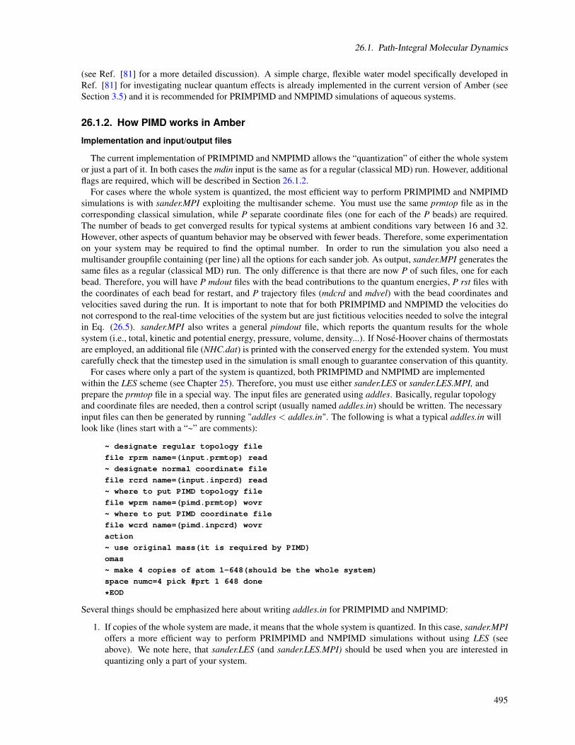
26.1. Path-Integral Molecular Dynamics
(see Ref. [81] for a more detailed discussion). A simple charge, flexible water model specifically developed inRef. [81] for investigating nuclear quantum effects is already implemented in the current version of Amber (seeSection 3.5) and it is recommended for PRIMPIMD and NMPIMD simulations of aqueous systems.
26.1.2. How PIMD works in Amber
Implementation and input/output files
The current implementation of PRIMPIMD and NMPIMD allows the “quantization” of either the whole systemor just a part of it. In both cases the mdin input is the same as for a regular (classical MD) run. However, additionalflags are required, which will be described in Section 26.1.2.
For cases where the whole system is quantized, the most efficient way to perform PRIMPIMD and NMPIMDsimulations is with sander.MPI exploiting the multisander scheme. You must use the same prmtop file as in thecorresponding classical simulation, while P separate coordinate files (one for each of the P beads) are required.The number of beads to get converged results for typical systems at ambient conditions vary between 16 and 32.However, other aspects of quantum behavior may be observed with fewer beads. Therefore, some experimentationon your system may be required to find the optimal number. In order to run the simulation you also need amultisander groupfile containing (per line) all the options for each sander job. As output, sander.MPI generates thesame files as a regular (classical MD) run. The only difference is that there are now P of such files, one for eachbead. Therefore, you will have P mdout files with the bead contributions to the quantum energies, P rst files withthe coordinates of each bead for restart, and P trajectory files (mdcrd and mdvel) with the bead coordinates andvelocities saved during the run. It is important to note that for both PRIMPIMD and NMPIMD the velocities donot correspond to the real-time velocities of the system but are just fictitious velocities needed to solve the integralin Eq. (26.5). sander.MPI also writes a general pimdout file, which reports the quantum results for the wholesystem (i.e., total, kinetic and potential energy, pressure, volume, density...). If Nosé-Hoover chains of thermostatsare employed, an additional file (NHC.dat) is printed with the conserved energy for the extended system. You mustcarefully check that the timestep used in the simulation is small enough to guarantee conservation of this quantity.
For cases where only a part of the system is quantized, both PRIMPIMD and NMPIMD are implementedwithin the LES scheme (see Chapter 25). Therefore, you must use either sander.LES or sander.LES.MPI, andprepare the prmtop file in a special way. The input files are generated using addles. Basically, regular topologyand coordinate files are needed, then a control script (usually named addles.in) should be written. The necessaryinput files can then be generated by running "addles < addles.in". The following is what a typical addles.in willlook like (lines start with a “~” are comments):
~ designate regular topology file
file rprm name=(input.prmtop) read
~ designate normal coordinate file
file rcrd name=(input.inpcrd) read
~ where to put PIMD topology file
file wprm name=(pimd.prmtop) wovr
~ where to put PIMD coordinate file
file wcrd name=(pimd.inpcrd) wovr
action
~ use original mass(it is required by PIMD)
omas
~ make 4 copies of atom 1-648(should be the whole system)
space numc=4 pick #prt 1 648 done
*EOD
Several things should be emphasized here about writing addles.in for PRIMPIMD and NMPIMD:
1. If copies of the whole system are made, it means that the whole system is quantized. In this case, sander.MPIoffers a more efficient way to perform PRIMPIMD and NMPIMD simulations without using LES (seeabove). We note here, that sander.LES (and sander.LES.MPI) should be used when you are interested inquantizing only a part of your system.
495

26. Quantum dynamics
2. The current implementation requires that the “omas” tag must be turned on to make every atom use originalmass during the simulation.
3. As mentioned above, how many copies to create is a tradeoff between accuracy and efficiency. To getconverged total energies, 16-32 copies may be required; however, other aspects of quantum behavior may beseen with fewer copies. Be prepared to experiment on your system to see what is required.
As output, sander.LES (and sander.LES.MPI) generates the same files as a regular (classical MD) run. The mdoutfile contains the quantum results for the whole system (i.e., total, kinetic and potential energy, pressure, volume,density...). while the rst file contains the coordinates of all beads for restart. The trajectory files (mdcrd and mdvel)contain the coordinates and velocities of all beads saved during the run. If Nosé-Hoover chains of thermostats areemployed, an additional file (NHC.dat) is printed with the conserved energy for the extended system. You mustcarefully check that the timestep used in the simulation is small enough to guarantee conservation of this quantity.
Input parameters
In order to perform PRIMPIMD and NMPIMD simulations, an additional flag is required in the mdin file, whichdistinguishes among the different methodologies based on the path-integral formalism.
ipimd Flag for the different methodologies based on the path-integral formalism. See Sections 26.2.1 and26.3.1 for the other values.
= 0 defines regular MD (default).
= 1 defines PRIMPIMD.
= 2 defines NMPIMD.
As described above, in order to guarantee a proper canonical sampling of the phase space the quantum systemmust be coupled to a thermostat. In the current implementation, two schemes are available: Langevin thermostatand Nosé-Hoover chains of thermostats coupled to each degree of freedom of the system. As for any regular MDrun, the flag that activates the thermostat is ntt. A Langevin thermostat is switched on using ntt=3, and defininga collision frequency. To activate the Nosé-Hoover chains of thermostats, you must specify ntt=4 and provide thenumber of thermostats (nchain) in each chain. Use of Nosé-Hoover chains of thermostats is rcommended and is theonly option currently available for NMPIMD (ipimd=2). The choice of an appropriate number of chains dependson the system. Typically, 4 thermostats (nchain=4) are sufficient to guarantee an efficient sampling of the phasespace.
In summary:
ntt Switch for temperature scaling. See Section 18.6.7 for other options.
= 3 defines a Langevin thermostat and also requires the definition of gamma_ln. Available forPRIMPIMD (ipimd=1) only.
= 4 defines Nosé-Hoover chains of thermostats. Available for PRIMPIMD (ipimd=1) and NMPIMD(ipimd=2). It also requires the number of thermostats in a chain (nchain).
nchain = 2-8 number of thermostats in each Nosé-Hoover chain of thermostats (default 2, recommended≥ 4).
Quantum simulations in the isothermic-isobaric (NPT) ensemble are possible only for NMPIMD (ipimd=2) andfor rectangular periodic boundary conditions (ntb=2) with isotropic position scaling (ntp=1). All the other flags areidentical to those for a classical MD simulation. The current implementation of NMPIMD for the NPT ensembleis based on the derivation of Ref [500].
Examples
In the following examples of input files for PRIMPIMD and NMPIMD are shown. You are also encouraged tocheck the test cases in $AMBERHOME/test/PIMD.
a) PRIMPIMD input for sander.LES. No periodic boundary conditions.
496

26.2. Centroid Molecular Dynamics (CMD)
Test: $AMBERHOME/test/PIMD/part_pimd_water.
ipimd = 1 ! PRIMPIMD
ntb = 0
ntx = 1, irest = 0
cut = 100.
temp0 = 300., tempi = 300., temp0les = -1.
ntt = 3, gamma_ln = 20. ! Langevin thermostat
dt = 0.0001, nstlim = 1000
ntpr = 100, ntwr = 1000, ntwx = 100
b) PRIMPIMD input for sander.LES. NVT simulation for water with only the hydrogen atoms being quantized.
Test: $AMBERHOME/test/PIMD/part_pimd_spcfw.
ipimd = 1 ! PRIMPIMD
ntx = 5, irest = 0
temp0 = 300., tempi = 300., temp0les = -1.
dt = 0.0002, nstlim 10
cut = 7.
ntt = 3, gamma_ln = 20. ! Langevin thermostat
ntpr = 1, ntwr = 10, ntwx = 1
c) NMPIMD input for sander.LES. NPT simulation for liquid butane.
Test: $AMBERHOME/test/PIMD/part_nmpimd_ntp.
ipimd = 2 ! NMPIMD
ntb = 2, ntp = 1 ! isotropic position scaling
ntx = 5, irest = 0
cut = 8.
temp0 = 80., tempi = 80., temp0les = -1.
ntt = 4, nchain = 4. ! Nose’-Hoover chains
dt = 0.0002, nstlim = 50
ntpr = 5, ntwr = 50, ntwx = 1
d) NMPIMD input for sander.MPI. NPT simulation for liquid water.
Test: $AMBERHOME/test/PIMD/full_pimd_ntp_water.
ipimd = 2 ! NMPIMD
ntb = 2, ntp = 1 ! isotropic position scaling
ntx = 5, irest = 1
cut = 7.
temp0 = 298.15
ntt = 4, nchain = 4. ! Nose’-Hoover chains
dt = 0.0002, nstlim = 10
ntpr = 1, ntwr = 10, ntwx = 5
26.2. Centroid Molecular Dynamics (CMD)
Two methods based on the path-integral formalism are available to perform approximate quantum dynamicalcalculations: Centroid Molecular Dynamics (CMD) [501] and Ring Polymer Molecular Dynamics (RPMD) [502].
The CMD method developed by Voth and coworkers draws upon the prescription of quantum distribution func-tions, in which the exact quantum expressions are cast into a phase space representation leading to a classical-like
497

26. Quantum dynamics
physical interpretation of the variables of interest. In particular, an approximate quantum dynamics is obtainedby propagating the centroid variables (i.e., positions and velocities of the center of mass of the bead polymer)according to classical-like equations of motion. The current implementation is the so-called Adiabatic CMD [503]that makes use of a normal mode representation of path-integrals where the fictitious mass of the zero-frequencymode (i.e., the centroid of the bead polymer) is given the actual mass of the atom and, contrary to NMPIMD, thefictitious masses of all the nonzero frequency modes are scaled by an adiabaticity parameter, γ < 0. This proceduredecouples the centroid motion from that of the other normal modes in the same spirit of the Car-Parrinello method.Although the centroid variables move following Newton’s equations of motion, Nosé-Hoover chains of thermostatsmust be attached to each nonzero frequency normal mode. The user is strongly encouraged to refer to the relevantliterature (Ref. [501] and references therein) for a more rigorous derivation of the CMD method.
The RPMD method developed by Manolopoulos and coworkers is based on primitive PIMD. However, thereare two fundamental differences: 1) each bead is given a fictitious mass equal to the actual mass of the atom (i.e.,µ = m), 2) the dynamics of the system is strictly determined by the fictitious Hamiltonian of Eq. (26.11), i.e., nothermostats are employed. Also in this case, the user is strongly encouraged to refer to the relevant literature for adetailed derivation of this method [502].
Both CMD and RPMD simulations provide an efficient route for the calculation of approximate Kubo trans-formed correlation functions, which can then be related to the true quantum correlation functions. Importantly,running several independent trajectories is required for both CMD and RPMD to guarantee a proper canonical av-erage of the initial conditions and, consequently, to obtain converged results (see Refs. [81] and[504] for examplesof CMD and RPMD simulations, respectively).
All the force fields available for regular MD simulations in Amber can be used for CMD and RPMD. However,we also note here that the common empirical force fields may require an additional reparameterization (see Ref.[81] for a more detailed discussion). A simple charge, flexible water model specifically developed in Ref. [81]for investigating nuclear quantum effects is already implemented in the current version of Amber (see Section 3.5)and it is recommended for CMD and RPMD simulations of aqueous systems.
26.2.1. Implementation and input/output files
The implementation of CMD and the input/output files are identical to those of NMPIMD (see Section26.1.2), with few differences. In addition to the NMPIMD output files, two other files are generated for CMD:CMD_position.dat containing the centroid positions, and CMD_velocity.dat containing the centroid velocitiessaved along the trajectory. The format of these files is identical to that of a classical MD simulation (mdcrdand mdvel), and the frequency with which these information are saved is determined by ntpr. The mdin input isthe same as for a regular (classical MD) run. However, additional flags are required as described below.
In order to perform CMD simulations the following flags are required in the mdin file:
ipimd Flag for the different methodologies based on the path-integral formalism. See Section 26.1.2 for theother values.
= 3 defines CMD.
adiab_param This defines the so-called adiabaticity parameter (γ) used to make the fictitious masses of the nonzerofrequency normal modes small enough to decouple their motion from that of the centroid. It has beenshown that γ ≤ 1/2P (where P is the total number of beads) is sufficiently small to get convergedresults. As a consequence of this, a smaller timestep is required. During the equilibration run (seebelow) you must carefully check that the timestep employed is small enough to guarantee the energyconservation of the extended system reported in the NHC.dat file (see Section 26.1.2). Default is 1,but you need to specify this, since default value is not appropriate.
ntt Switch for temperature scaling.
= 4 defines Nosé-Hoover chains of thermostats. It also requires the number of thermostats in a chain(nchain). For CMD, Nosé-Hoover chains of thermostats must be attached to each nonzero fre-quency normal mode.
nchain = 2-8 number of thermostats in each Nosé-Hoover chain of thermostats (default 2, recommended≥ 4).
498

26.2. Centroid Molecular Dynamics (CMD)
eq_cmd This flag must be used during the CMD equilibration to generate a canonical distribution of the cen-troid variables before an actual CMD run. Default is .false.
restart_cmd Flag necessary for restarting a CMD simulation.
In order to run a CMD simulation, you must first generate an equilibrated quantum configuration of your systemusing NMPIMD (see Section 26.1.2). A canonical distribution of the centroid variables must then be obtainedfrom a CMD simulation with the equilib_cmd flag on. After this equilibration, the final configuration is then usedas initial configuration for the actual CMD simulation. For restarting a CMD run the restart_cmd flag in the mdinfile is required.
Importantly, for CMD simulations it is necessary that ntb=1, which is the default value.
26.2.2. Examples
In the following examples of input files for CMD are shown. You are also encouraged to check the test cases in$AMBERHOME/test/PIMD.
a) CMD for sander.LES. Equilibration of the centroid variables.
Test: $AMBERHOME/test/PIMD/part_cmd_water/equilib.
ipimd = 3 ! CMD
ntx = 5, irest = 0
ntb = 1
temp0 = 298.15, tempi = 298.15, temp0les = -1.
cut = 7.0
ntt = 4, nchain = 4. ! Nose’-Hoover chains
dt = 0.00005, nstlim = 100
eq_cmd = .true. ! equilibration for CMD
adiab_param = 0.5 ! adiabaticity parameter
ntpr = 20, ntwr = 100
b) CMD input for sander.LES. Start of an actual CMD simulation after equilibration.
Test: $AMBERHOME/test/PIMD/part_cmd_water/start.
ipimd = 3 ! CMD
ntx = 5, irest = 1
ntb = 1
temp0 = 298.15, tempi = 298.15, temp0les = -1.
cut = 7.0
ntt = 4, nchain = 4. ! Nose’-Hoover chains
dt = 0.00005, nstlim = 100
eq_cmd = .false. ! actual CMD
adiab_param = 0.5 ! adiabaticity parameter
ntpr = 20, ntwr = 100
c) CMD input for sander.LES. Restart of an actual CMD.
Test: $AMBERHOME/test/PIMD/part_cmd_water/restart.
ipimd = 3 ! CMD
ntx = 5, irest = 1
ntb = 1
temp0 = 298.15, tempi = 298.15, temp0les = -1.
cut = 7.0
499
26. Quantum dynamics
ntt = 4, nchain = 4. ! Nose’-Hoover chains
dt = 0.00005, nstlim = 100
eq_cmd = .false. ! actual CMD
restart_cmd = .true. ! restart
adiab_param = 0.5 ! adiabaticity parameter
ntpr = 20, ntwr = 100
26.3. Ring Polymer Molecular Dynamics (RPMD)
The implementation of RPMD and the necessary input/output files are identical to those of PRIMPIMD (seeSection 26.1.2). The mdin input is the same as for a PRIMPIMD with only few differences described below.
26.3.1. Input parameters
In order to perform RPMD the following flags are required in the mdin file:
ipimd Flag for the different methodologies based on the path-integral formalism. See Section 26.1.2 for theother values.
= 4 defines RPMD.
ntt Set this to 0, for constant energy dynamics
nscm Set this to 0, to avoid removing translational and rotational center-of-mass motion.
You must first generate an equilibrated quantum configuration of your system using PRIMPIMD (see Section26.1.2), which is then used as initial configuration for the actual RPMD simulation.
26.3.2. Examples
In the following examples of input files for RPMD are shown. You are also encouraged to check the test casesin $AMBERHOME/test/PIMD.
a) RPMD input for sander.LES.
Test: $AMBERHOME/test/PIMD/part_rpmd_water.
ipimd = 4 ! RPMD
ntx = 5, irest = 0
ntt = 0
nscm = 0
temp0 = 300., temp0les = -1.
cut = 7.0
dt = 0.0002, nstlim = 10
ntpr = 1, ntwr = 10, ntwx = 1, ntwv = 1
26.4. Linearized semiclassical initial value representation
26.4.1. Experimental observables and thermal correlation functions
Most quantities of interest in the dynamics of complex systems can be expressed in terms of thermal timeautocorrelation functions [505], which are of the form
CAB (t) =1Z
Tr(
Aβ eiHt/hBe−iHt/h)
(26.12)
500
26.4. Linearized semiclassical initial value representation
where Aβ
std = e−β H A for the standard version of the correlation function, or Aβsym = e−β H/2Ae−β H/2 for the sym-
metrized version [506], or
Aβ
Kubo =1β
∫β
0dλe−(β−λ )H Ae−λ H (26.13)
for the Kubo-transformed version [507]. These three versions are related to one another by the following identitiesbetween their Fourier transforms,
β hω
1− e−β hωIKuboAB (ω) = Istd
AB (ω) = eβ hω/2IsymAB (ω) (26.14)
where
IAB (ω) =
∞∫−∞
dt e−iωtCAB (t) (26.15)
is the partition function and H the (time-independent) Hamiltonian of the system, and A and B are operatorsrelevant to the specific property of interest.
26.4.2. Linearized semiclassical initial value representation
The Semiclassical initial value representation (SC-IVR) approximates the forward (backward) time evolutionoperator e−iHt/h (eiHt/h) by a phase space average over the initial conditions of forward (backward) classicaltrajectories [508, 509]. By making the approximation that the dominant contribution to the phase space averagescomes from forward and backward trajectories that are infinitesimally close to one another, and then linearizing thedifference between the forward and backward actions (and other quantities in the integrand), Miller and coworkers[510, 511] obtained the LSC-IVR, or classical Wigner model for the correlation function in Eq. (26.12),
CLSC−IV RAB (t) = Z−1 (2π h)−N
∫dx0
∫dp0Aβ
w (x0,p0)Bw (xt ,pt) (26.16)
where Aβw and Bw are the Wigner functions corresponding to these operators,
Ow (x,p) =∫
dx〈x−∆x/2| O |x+∆x/2〉ei pT ∆x/h (26.17)
for any operator O . Here N is the number of degrees of freedom in the system, and (x0,p0) is the set of initialconditions (i.e., coordinates and momenta) for a classical trajectory, (x(x0,p0) ,pt (x0,p0)) being the phase pointat time along this trajectory. It should also be noted that there are other approximate routes which lead to theclassical Wigner model for correlation functions (other than simply postulating it). [Please see Section II-A ofRef. [512] or Section III-A of Ref. [513] for more discussion.] The LSC-IVR can be shown to be exact in theclassical limit (→ 0), high temperature limit (β → 0), and harmonic limit [514]. The LSC-IVR can treat bothlinear and nonlinear operators in a consistent way [515], can be applied to non-equilibrium as well as the aboveequilibrium correlation functions, and can also be used to describe electronically non-adiabatic dynamics, i.e.,processes involving transitions between several potential energy surfaces. These merits of the LSC-IVR make it aversatile tool to study a variety of quantum mechanical effects in chemical dynamics of large molecular systems.
26.4.3. Local Gausssian approximation
Calculation of the Wigner function for operator B in Eq. (26.16) is usually straight-forward; in fact, is oftena function only of coordinates or only of momenta, in which case its Wigner functions is simply the classicalfunction itself. Calculating the Wigner function for operator Aβ however, involves the Boltzmann operator withthe total Hamiltonian of the complete system, so that carrying out the multidimensional Fourier transform to obtainit is far from trivial. Furthermore, it is necessary to do this in order to obtain the distribution of initial conditions ofmomenta for the real time trajectories. To accomplish this task, the local Gaussian approximation (LGA) proposedby Liu and Miller [512], which can be viewed as an improved version of the local harmonic approximation (LHA),
501

26. Quantum dynamics
[516] and which is able to consistently treat the entire imaginary frequency regime, has been implemented inAmber. Below we briefly summarize the LGA. As in the standard normal-mode analysis, mass-weighted Hessianmatrix elements are given by
Hkl =1
√mkml
∂ 2V∂xk∂xl
(26.18)
where represent the mass of the k-th degree of freedom. The eigenvalues of the mass-weighted Hessian matrixproduce normal-mode frequencies ωk i.e.,
THT = λ (26.19)
with λ a diagonal matrix with the elements(ωk)
2
and T an orthogonal matrix. If is the diagonal ‘mass matrix’with elements mk , then the mass-weighted normal mode coordinates and momenta (X0,P0) are given in termsof the Cartesian variables (x0,p0) by
X0 = TT M1/2x0 (26.20)
andP0 = TT M−1/2p0 (26.21)
The Fourier transform of Eq. (26.17) then gives the Wigner function of as
Aβw (x0,p0) = (2π h)N 〈x0|e−β H |x0〉
×N
∏k=1
[(β
2πQ(uk)
)1/2
exp
[−β
(P0,k)2
2Q(uk)
]]fA (x0,p0) (26.22)
where uk = β hωk , P0,k is the k-th component of the mass-weighted normal-mode momentum in Eq. (26.21) andthe quantum correction factor is given by
Q(u) =
u/2
tanh(u/2)f or real u
=1
Q(ui)=
tanh(ui/2)ui/2
f or imaginaryu (u = iui)
(26.23)
In Eq. (26.22),
fA (x0,p0) =
∫dx 〈x0− ∆x
2 |Aβ |x0+∆x2 〉
〈x0|e−β H |x0〉ei∆xT ·p0/h
∫d∆x 〈x0− ∆x
2 |e−β H |x0+∆x2 〉
〈x0|e−β H |x0〉ei∆xT ·p0/h
(26.24)
is a function depending on the operator Aβ . For example, when Aβ = e−β H x , one has
fA (x0,p0) = x0 +iβ h2
M−1/2TQ(u)−1 P0 (26.25)
where is the diagonal quantum correction factor matrix with the elements Qk ≡ Q(uk) . Using Eq. (26.24), onecan figure out the quantity fA (x0,p0) for different operators Aβ .
The explicit form of LSC-IVR correlation function (Eq. (26.16)) with the LGA is thus given by
CLSC−IV RAB (t) =
1Z
∫dx0 〈x0|e−β H |x0〉
∫dP0
N
∏k=1
[(β
2πQ(uk)
)1/2
exp
[−β
(P0,k)2
2Q(uk)
]]× fA (x0,p0)B(xt ,pt)
(26.26)
Please refer to Refs. [512] and [513] for more detail about the LSC-IVR and the LGA.
502
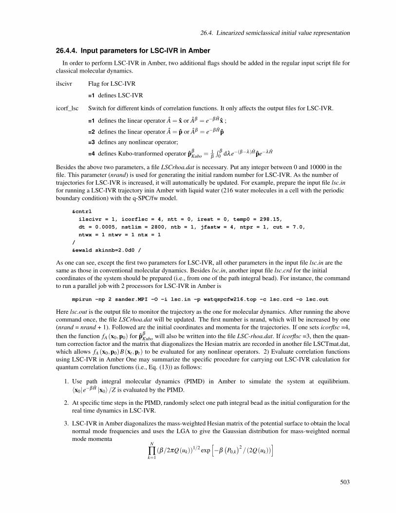
26.4. Linearized semiclassical initial value representation
26.4.4. Input parameters for LSC-IVR in Amber
In order to perform LSC-IVR in Amber, two additional flags should be added in the regular input script file forclassical molecular dynamics.
ilscivr Flag for LSC-IVR
=1 defines LSC-IVR
icorf_lsc Switch for different kinds of correlation functions. It only affects the output files for LSC-IVR.
=1 defines the linear operator A = x or Aβ = e−β H x ;
=2 defines the linear operator A = p or Aβ = e−β H p=3 defines any nonlinear operator;
=4 defines Kubo-tranformed operator pβ
Kubo =1β
∫ β
0 dλe−(β−λ )H pe−λ H
Besides the above two parameters, a file LSCrhoa.dat is necessary. Put any integer between 0 and 10000 in thefile. This parameter (nrand) is used for generating the initial random number for LSC-IVR. As the number oftrajectories for LSC-IVR is increased, it will automatically be updated. For example, prepare the input file lsc.infor running a LSC-IVR trajectory inin Amber with liquid water (216 water molecules in a cell with the periodicboundary condition) with the q-SPC/fw model.
&cntrl
ilscivr = 1, icorflsc = 4, ntt = 0, irest = 0, temp0 = 298.15,
dt = 0.0005, nstlim = 2800, ntb = 1, jfastw = 4, ntpr = 1, cut = 7.0,
ntwx = 1 ntwv = 1 ntx = 1
/
&ewald skinnb=2.0d0 /
As one can see, except the first two parameters for LSC-IVR, all other parameters in the input file lsc.in are thesame as those in conventional molecular dynamics. Besides lsc.in, another input file lsc.crd for the initialcoordinates of the system should be prepared (i.e., from one of the path integral bead). For instance, the commandto run a parallel job with 2 processors for LSC-IVR in Amber is
mpirun -np 2 sander.MPI -O -i lsc.in -p watqspcfw216.top -c lsc.crd -o lsc.out
Here lsc.out is the output file to monitor the trajectory as the one for molecular dynamics. After running the abovecommand once, the file LSCrhoa.dat will be updated. The first number is nrand, which will be increased by one(nrand = nrand + 1). Followed are the initial coordinates and momenta for the trajectories. If one sets icorflsc =4,then the function fA (x0,p0) for pβ
Kubo will also be written into the file LSC-rhoa.dat. If icorflsc =3, then the quan-tum correction factor and the matrix that diagonalizes the Hesian matrix are recorded in another file LSCTmat.dat,which allows fA (x0,p0)B(xt ,pt) to be evaluated for any nonlinear operators. 2) Evaluate correlation functionsusing LSC-IVR in Amber One may summarize the specific procedure for carrying out LSC-IVR calculation forquantum correlation functions (i.e., Eq. (13)) as follows:
1. Use path integral molecular dynamics (PIMD) in Amber to simulate the system at equilibrium.〈x0|e−β H |x0〉/Z is evaluated by the PIMD.
2. At specific time steps in the PIMD, randomly select one path integral bead as the initial configuration for thereal time dynamics in LSC-IVR.
3. LSC-IVR in Amber diagonalizes the mass-weighted Hesian matrix of the potential surface to obtain the localnormal mode frequencies and uses the LGA to give the Gaussian distribution for mass-weighted normalmode momenta
N
∏k=1
(β/2πQ(uk))1/2 exp
[−β(P0,k)2/(2Q(uk))
]
503

26. Quantum dynamics
Illustration of the LSC‐IVR
Imaginary time
Randomly/Sequentially
select one of the path
integral beads as the
initial configuration x,
and then generate
initial momentum p
PIMD interval t_im PIMD interval t_im
Real tim
eclassical trajecto
ry
Real tim
e classical trajecto
ry
Imaginary time
Collect the estimators
from this trajectory for the
correlation functions
Collect the estimators
from this trajectory for the
correlation functions
Randomly/Sequentially
select one of the path
integral beads as the
initial configuration x,
and then generate
initial momentum p
Figure 26.1.: Flow chart for LSC-IVR.
which is used to randomly sample initial Cartesian momentum p0 = M1/2T P0 for the real time trajectory.Notice the parameter nrand in the file LSCrhoa.dat is used. LSC-IVR in Amber further runs a trajectoryfrom the phase space point (x0,p0) . As in conventional molecular dynamics, the output files mdcrd andmdvel record the trajectory (xt (x0,p0) ,pt (x0,p0)). The parameter nrand is updated in the file LSCrhoa.dat,with the initial phase point (x0,p0) the mass, and fA (x0,p0) for pβ
Kubo , etc. The file LSCTmat.dat may alsobe created for the quantum correction factor and the matrix .
4. The propertyfA (x0,p0)B(xt (x0,p0) ,pt (x0,p0))
for the corresponding time correlation function can be evaluated for the trajectory with the output files(mdcrd, mdvel, LSCrhoa.dat and LSCTmat.dat). One can write a short program in order to do so.
5. Repeat steps 2)-4) and sum the property
fA (x0,p0)B(xt (x0,p0) ,pt (x0,p0))
for all real time classical trajectories until a converged result is obtained. It is worth noting that one can alsosequentially select one path integral bead as the initial configuration in Step 2) each turn. Also in Step 4),one can simultaneously evaluate different
fA (x0,p0)B(xt (x0,p0) ,pt (x0,p0))
for different correlation functions.
Here we give an example for the script file to get one real time trajectory in LSC-IVR for the water systemalready at equilibrium. (216 water molecules in a cell with the periodic boundary condition, 24 path integralbeads used for the PIMD).
## This is to run PIMD for short time
mpirun -np 24 sander.MPI -ng 24 -groupfile gfpimd > sander.out
504

26.5. Reactive Dynamics
## Copy the configuration of one path integral bead
cd ..
cp -p PIMD/pimdbead1.rst LSC/lsc.crd
## This is to run LSC to get a real time trajectory
cd LSC
mpirun -np 2 sander.MPI -O -i lsc.in -p watqspcfw216.top -c lsc.crd -o lsc.out
## a.out is the executable file that the user writes to calculate
## for correlation functions of his/her own interest
./a.out
Here the file gfpimd is like
-O -i pimd.in -p watqspcfw216.top -c pimdbead1.rst -o pimdbead1.out
-r pimdbead1.rst -pimdout pimd.out
-O -i pimd.in -p watqspcfw216.top -c pimdbead2.rst -o pimdbead2.out
-r pimdbead2.rst -pimdout pimd.out
......
-O -i pimd.in -p watqspcfw216.top -c pimdbead24.rst -o pimdbead2.out
-r pimdbead2.rst -pimdout pimd.out
For collecting many LSC-IVR trajectories, one can repeatedly use the commands in the script file with the onlychange for sequentially copying a path integral bead for the initial configuration for LSC-IVR, i.e.,
cp -p PIMD/pimdbead*.rst LSC/lsc.crd
Here "*" is replaced by one of the numbers 1-24 each time circularly.All the force fields available for conventional molecular dynamics in Amber can be used for LSC-IVR. However,
one should also keep in mind that some empirical force fields may require additional reparameterization (such asq-SPC/fw for SPC/fw) for approximated quantum dynamical methods such as LSC-IVR, CMD and RPMD.
26.5. Reactive Dynamics
26.5.1. Path integral quantum transition state theory
The path integral quantum transition state theory rate [517] is given by
kPI−QTST = 1/2⟨∣∣∣ξ ∣∣∣⟩
ξ ‡ρc(ξ
‡) (26.27)
where the centroid density
ρc (ξ ) =
∫dr(1)dr(2) · · ·dr(P) exp
[−βΦ(r(1), . . . ,r(P))
]δ
[ξc(r(1), . . . ,r(P))−ξ
]∫
dr(1)dr(2) · · ·dr(P) exp[−βΦ(r(1), . . . ,r(P))
]h[ξ ‡− ξc(r(1), . . . ,r(P))
] (26.28)
is related to the potential of mean force w(ξ ) as
ρc (ξ ) =exp [−βw(ξ )]∫ ξ ‡
−∞ dξ exp [−βw(ξ )](26.29)
In Eq. (26.28), β = 1/kBT , Φ is the effective potential (see Eqs. 26.8 and 26.49), h is the Heaviside step function,ξ ‡ is the location of the dividing surface that partitions the reactant and product regions and ξc is the value of the
reaction coordinate as a function of the centroid coordinates r(c) = 1P
P
∑s=1
r(s). As Eq. (26.29) suggests, the centroid
density factor can be computed using umbrella sampling approaches to generate a set of biased distributions thatthen can be combined into a PMF using the WHAM approach [245–247]. The dynamical frequency factor can beapproximated by the velocity of a free particle along the reaction coordinate direction
505
26. Quantum dynamics
⟨∣∣∣ξ ∣∣∣⟩ξ ‡
=
(2
πβ
)1/2⟨ 3N
∑i=1
1mi
(∂ ξc
∂ r(c)i
)21/2⟩
ξ ‡
(26.30)
where 〈· · · 〉ξ ‡ denotes the conditional average computed at the dividing surface ξ ‡. Both factors in the PI-QTST
rate expression can be computed using the EVB/LES-PIMD facility in Amber (see Section 8.4). The value of thecentroid reaction coordinate and the velocity of a free particle along the centroid RC direction are written to thefile evbout. To output
∣∣∣ξ ∣∣∣, set the variable out_RCdot = .true. in the EVB input file.
26.5.2. Quantum Instanton
The Quantum Instanton (QI) is a theoretical approach for computing thermal reaction rates in complex molecu-lar systems, which is related to an older semiclassical (SC) theory of reaction rates that came to be known as the“instanton” approximation[518]. The SC instanton approximation is based on a SC approximation for the Boltz-mann operator, exp(−βH), which involves a classical periodic orbit in pure imaginary time (or equivalently in realtime on the upside-down potential energy surface) plus harmonic fluctuations about it[518]. The essential featureof the QI rate constant [519] is that it is expressed wholly in terms of the quantum Boltzmann operator, which canbe evaluated for complex molecular systems using the path-integral methods described in Sec. 26.1.
In the following we will briefly illustrate the basic principles, and we will derive the fundamentals of the QIapproach. We strongly recommend the user to consult the relevant literature for a more rigorous description[519,520].
The derivation begins with the following formally exact expression of the quantum mechanical thermal rateconstant[518]:
k(T )Qr(T )≡ kQr =1
2π
∫dEe−βEN(E), (26.31)
where Qr(T ) is the reactant partition function per unit volume at temperature T, β is the inverse temperature 1/kBT ,and N(E) is the cumulative reaction probability at total energy E[506]:
N(E) =(2π)2
2tr[Faδ
(E− H
)Fbδ
(E− H
)]. (26.32)
In Eq. 26.32 the flux operators Fa and Fb are defined by
Fγ =i[H,h
(ξγ (q)
)], (26.33)
where γ = a,b, h(ξγ
)is the Heaviside function, and His the Hamiltonian of the system. We note that Eqs. 26.32
and 26.33 involve two dividing surfaces ξa (q) = 0 and ξb (q) = 0. The microcanonical density operator δ(E− H
)in Eq. 26.32 as well as the integral over the total energy in Eq. 26.31 can be computed using a semiclassicalapproximation, which results in the following quantum instanton expression for the rate constant:
k ' kQI ≡1
QrC f f (0)
√π
2
∆H. (26.34)
In Eq. 26.34, C f f (0) is the zero time value of the flux-flux correlation function generalized to the case of twoseparate dividing surfaces,
C f f (t) = tr[e−β H/2Fae−β H/2eiHt/Fbe−iHt/
], (26.35)
and ∆H is a specific type of energy variance given by
506

26.5. Reactive Dynamics
∆H2 =tr[∆ae−β H/2H2∆be−β H/2
]− tr
[∆ae−β H/2H∆be−β H/2H
]tr[∆ae−β H/2∆be−β H/2
] (26.36)
with ∆a and ∆bbeing a modified version of the Dirac delta function:
∆γ = ∆(ξγ (q)
)≡ δ
(ξγ (q)
)| m−1/2Oξγ (q) | (26.37)
where γ = a,b. It has been shown that ∆H can also be expressed in terms of the “delta-delta” correlationfunction[520].
The QI rate constant [Eq. (26.34)] can be rewritten in the form [520]
kQI =Cdd(0)
Qr
C f f (0)Cdd(0)
√π
2h4H
(26.38)
where
Cdd(0;ξa,ξb)
Qr=
∫dr(1)dr(2) · · ·dr(P) exp
[−βΦ(r(1), . . . ,r(P))
]δ
[ξ (r(P))−ξa
]δ
[ξ (r(P/2))−ξb
]∫
dr(1)dr(2) · · ·dr(P) exp[−βΦ(r(1), . . . ,r(P))
]h[ξ ‡− ξ (r(P))
]h[ξ ‡− ξ (r(P/2))
] (26.39)
C f f (0)/Cdd(0) =⟨
fv
(r(1), . . . ,r(P)
)⟩ξ
‡(P),ξ
‡(P/2)
(26.40)
4H2 =12
⟨F(
r(1), . . . ,r(P))2
+G(
r(1), . . . ,r(P))⟩
ξ‡(P),ξ
‡(P/2)
(26.41)
The conditional average 〈· · · 〉ξ
‡(P),ξ
‡(P/2)
is computed from the ensemble sampled with the P and P/2 slices con-
strained to the dividing surface
〈· · · 〉ξ
‡(P),ξ
‡(P/2)
=
∫dr(1)dr(2) · · ·dr(P) exp
[−βΦ(r(1), . . . ,r(P))
]δ
[ξ (r(P))−ξa
]δ
[ξ (r(P/2))−ξb
]× (· · ·)∫
dr(1)dr(2) · · ·dr(P) exp[−βΦ(r(1), . . . ,r(P))
]δ
[ξ (r(P))−ξa
]δ
[ξ (r(P/2))−ξb
]where the quantities within the average (for the simple case of a single quantized nuclear particle) are defined asfollows:
fv
(r(1), . . . ,r(P)
)= m
(iP
2hβ
)2
∇ξa
(r(P))·(
r(1)− r(P−1))×∇ξb
(r(P/2)
)·(
r(P/2+1)− r(P/2−1))
(26.42)
F(
r(1), . . . ,r(P))=− mP
h2β 2
P/2
∑k=1−
P
∑k=P/2+1
(r(k)− r(k−1)
)2+
2P
P/2−1
∑k=1−
P−1
∑k=P/2+1
V(
r(k))
(26.43)
G(
r(1), . . . ,r(P))=
2dPβ 2 −
4mPh2
β 3
P
∑k=1
(r(k)− r(k−1)
)2(26.44)
All factors needed to calculate the QI rate can be obtained from the EVB/LES-PIMD facility in Amber (seeSection 8.4). For example, the joint distribution function [Eq. (26.39)] is computed using umbrella samplingalong the reaction coordinates of the P and P/2 slices. The DG EVB input file of the RS malonaldehyde systemmay contain the following specifications:
507

26. Quantum dynamics
&evb nevb = 2, nUFF = 1, nbias = 2, ntw_evb = 50,
dia_type = "ab_initio",
xch_type = "dist_gauss",
evb_dyn = "qi_dbonds_pmf",
dia_shift(1)%st = 1, dia_shift(1)%nrg_offset = 0.0,
dia_shift(2)%st = 2, dia_shift(2)%nrg_offset = 0.0,
dbonds_umb(1)%iatom = 8, dbonds_umb(1)%jatom = 9, dbonds_umb(1)%katom = 7,
dbonds_umb(1)%k = 100.0, dbonds_umb(1)%ezero = -.20,
dbonds_umb(2)%iatom = 8, dbonds_umb(2)%jatom = 9, dbonds_umb(2)%katom = 7,
dbonds_umb(2)%k = 100.0, dbonds_umb(2)%ezero = .40,
dist_gauss%stype = "no_dihedrals",
dist_gauss%lin_solve = "diis",
dist_gauss%xfile_type = "gaussian_fchk",
ts_xfile(1) = "malonaldehydeTS_35.fchk",
min_xfile(1) = "malonaldehydeR_35.fchk",
min_xfile(2) = "malonaldehydeP_35.fchk",
dgpt_alpha(1) = 0.72,
dgpt_alpha(2) = 0.72,
dgpt_alpha(3) = 0.72,
UFF(1)%iatom = 7, UFF(1)%jatom = 9
/
where the variable evb_dyn = "qi_dbonds_pmf" requests biased sampling along a difference of distances RC onthe P and P/2 slices whose umbrella parameters are specified in dbonds_umb(:). Input specifications for the PSmalonaldehyde system is identical to the above, except that the UFF atom pair has been changed to reflect theproduct topology (see Section 8.5). A set of 2-dimensional (2D) biased simulations, each enhancing the samplingnear a particular point of the 2D (ξP× ξP/2) configuration space is required to map out the QI joint distribution.Using the WHAM procedure, the generated biased distributions can be unbiased to form Cdd(0)/Qr on the EVBground-state surface Vel0. All remaining factors involve conditional averages of fv, F and G. These quantities arecomputed using umbrella sampling with the P and P/2 slices constrained to the dividing surface ξ ‡ = 0.0 andare written to the evbout file. The corresponding EVB input file is identical to the above, but with the followingmodifications:
...
evb_dyn = "qi_dbonds_pmf",
evb_dyn = "qi_dbonds_dyn",...
dbonds_umb(1)%k = 100.0, dbonds_umb(1)%k = -.20,
dbonds_umb(1)%k = 400.0, dbonds_umb(1)%ezero = 0.0,...dbonds_umb(2)%k = 100.0, dbonds_umb(2)%ezero = .40,
dbonds_umb(2)%k = 400.0, dbonds_umb(2)%ezero = 0.0,...
26.6. Isotope effects
26.6.1. Thermodynamic integration with respect to mass
As mentioned in Section 22.1, the standard implementation of thermodynamic integration in Amber assumesthat the potential energy surface (PES) changes, but masses do not. For isotope effects the situation is exactly
508

26.6. Isotope effects
opposite: Within the Born-Oppenheimer approximation, the PES remains unchanged and it is the masses thatchange. One is usually interested in the ratio of the partition functions of the system with the heavy isotope (Q(h))and the light isotope (Q(l)),
Q(h)/Q(l) = e−β∆F ,
where the change in free energy ∆F can be computed by the thermodynamic integration (TI) with respect to massas
∆F =∫ 1
0〈dVeff(λ )/dλ 〉dλ . (26.45)
The parameter λ interpolates between the masses of the system with the lighter (λ = 0) and the heavier (λ = 1)isotopes,
mi(λ ) = (1−λ )m(l)i +λm(h)
i , (26.46)
and the effective potential Veff is defined as
Veff(λ ) :=−β−1 logQ(λ ) . (26.47)
The TI consists in running several simulations for different values of λ , computing 〈dVeff(λ )/dλ 〉 in each simula-tion, and performing the simple integral (Eq. 26.45) in the end.
In classical mechanics, the TI w.r.t. mass would be rather trivial, so we assume that the calculation is quantum-mechanical and uses PIMD. Let N be the number of atoms and P the number of imaginary time slices in thediscretized path integral (PI). (P = 1 gives classical mechanics, P→ ∞ gives quantum mechanics.) The PI repre-sentation of Q is
Q'(
P2π h2
β
)3NP/2 N
∏i=1
m3P/2i
∫dr(1) · · ·
∫dr(P)e−βΦ, (26.48)
where Φ is given by
Φ =P
2h2β 2
N
∑i=1
mi
P
∑s=1
(r(s)i − r(s+1)
i
)2+
1P
P
∑s=1
V(
r(s))
(26.49)
and r(s)i denotes the sth slice coordinates of the ith atom.The tricky part in PI simulations is finding efficient ways to estimate relevant quantities (in the PI jargon, finding
efficient “estimators”) – in our case dVeff(λ )/dλ from Eq. (26.45). For example, direct differentiation of Eq.(26.48) gives the thermodynamic-like estimator (TE),[521]
dVeff(λ )
dλ'−
N
∑i=1
dmi
dλ
[3P
2miβ− P
2h2β 2
P
∑s=1
(r(s)i − r(s+1)
i
)2]
(TE). (26.50)
The problem with this estimator is that its statistical error grows with P. If one wishes to go to the quantum limit,one must increase the number of samples enormously. In Ref. [522], this drawback was avoided by subtracting thecentroid coordinate
r(C)i =
1P
P−1
∑s=0
r(s)i
and using mass-scaled coordinates in Eq. (26.48). The resulting virial-like estimator (VE),
dVeff(λ )
dλ'−
N
∑i=1
dmi/dλ
mi
32β
+1
2P
⟨P
∑s=1
(r(s)i − r(C)
i
)·
∂V(
r(s))
∂r(s)i
⟩ (VE), (26.51)
has the advantage that the statistical error is independent of P. Compared to TE, the virial-like estimator requiresthe gradient of the potential, but at no additional cost, since the gradient is already needed for the PIMD. Bothtypes of estimators are implemented in Amber in order to provide an independent comparison, but in general thevirial estimator is preferred.
509

26. Quantum dynamics
Strictly speaking, the preceding derivation was for a system bound in an external potential. In molecular systemswith internal interactions only, the partition function can only be defined per unit volume because the center-of-mass coordinate is unbound. However, if the sampling is done in Cartesian coordinates as in Amber, the precedingestimators remain unchanged. This can be justified by considering a finite volume V and taking a limit V → ∞.
26.6.2. Amber implementation
The thermodynamic integration w.r.t. mass is run in Amber as any other PIMD simulation with the followingchanges.
1. In the mdin file, ITIMASS and CLAMBDA must be set.
ITIMASS = 0 No thermodynamic integration w.r.t. mass (default).
ITIMASS = 1 Run TI w.r.t. mass using the efficient virial estimator (26.51). This is the preferred value.
ITIMASS = 2 Run TI w.r.t. mass using the simple thermodynamic estimator (26.50). This option shouldonly be used for testing. The virial estimator (option 1) has much smaller statistical error.
CLAMBDA Contains the value of λ for TI (0.0≤ λ ≤ 1.0) from Eq. (26.46).
2. In the prmtop (topology) file, a flag TI_MASS with the perturbed masses must be added. In other words,the current flag MASS includes the masses for the first (unperturbed) isotopic system (m(l)
i ), and TI_MASSincludes the masses for the second (perturbed) isotopic system (m(h)
i ). Note that unlike the standard TI forwhich the force field changes, the TI w.r.t. mass requires only one topology file.
3. The output dVeff/dλ from Eqs. (26.50) and (26.51) for the TI is printed as “DV/DL” in the mdout file (asfor the standard TI).
Note: Currently, the TI w.r.t. mass can be used with both implementations of the PIMD (that is the full PIMD andthe LES PIMD). There are examples of both in the directory test/ti_mass.
26.6.3. Equilibrium isotope effects
Equilibrium (or thermodynamic) isotope effect (EIE) is the effect of isotopic substitution on the equilibriumconstant K of a chemical reaction. Denoting the quantities pertaining to the reaction with the lighter (heavier)isotope by a superscript l (h), the EIE is defined as the ratio of the equilibrium constants
EIE :=K(l)
K(h). (26.52)
Within the Born-Oppenheimer approximation, the potential energy surfaces of isotopic molecules are identical,and so the EIE is only due to the effect of the isotopic mass on the nuclear motion of the reactants and products.The EIE can be expressed as the ratio
EIE =Q(l)
p /Q(h)p
Q(l)r /Q(h)
r
. (26.53)
where Qr and Qp denote the reactant and product partition functions, respectively. Equation (26.52) suggests thatthe EIE can be found in practice by performing two thermodynamic integrations: for the reactants, Q(l)
r /Q(h)r , and
for the products, Q(l)p /Q(h)
p .
26.6.4. Kinetic isotope effects
Similarly, the kinetic isotope effect (KIE) is the effect of isotopic substitution on the rate constant k of a chemicalreaction, and is defined as
KIE :=k(l)
k(h).
510

26.6. Isotope effects
-0.5 0 0.5
Difference of Bond Lengths [Å]
0
0.5
1
1.5
2
Pote
ntia
l of
Mea
n Fo
rce
[kca
l/mol
]
Figure 26.2.: PMFs for proton ( curve) and deuterium (H curve) transfer in malonaldehyde using DG EVB/LES-PIMD.
The exact quantum-mechanical expression for the rate constant is
k = Q−1r tr
(e−β H FP
)where H is the Hamiltonian operator and FP is the reactive flux operator. Unfortunately, the exact k cannotbe computed even for fairly small molecules. There exists, however, a very accurate Quantum Instanton (QI)approximation for the rate constant [519], given by
kQI =12√
π hCff (0)Qr∆H
. (26.54)
In this expression, C f f (t) is the flux-flux correlation function and ∆H is a specific type of energy variance, definedin Ref. [519]. A path-integral implementation of the QI approximation to compute KIEs has been developed inRefs. [521] and [522]. Within this approximation, the KIE is written as a product of several factors,
KIEQI =k(l)QI
k(h)QI
=Q(l)
r
Q(h)r
× ∆H(h)
∆H(l)×
C(l)dd (0)
C(h)dd (0)
×C(l)
ff (0)/C(l)dd (0)
C(h)ff (0)/C(h)
dd (0), (26.55)
where for convenience we have multiplied and divided by so-called delta-delta correlation function Cdd (t). Usingthe PIMD implementation in Amber, quantities such as ∆H(h) or C(l)
ff (0)/C(l)dd (0), can be computed directly in a
constrained PIMD simulation because they are thermodynamic averages (see Section 26.5.2 on the QI evaluationof the rate constant). The ratio Q(l)
r /Q(h)r must be computed by the TI with respect to mass. Finally, the correlation
function Cdd (t) is defined very similarly to the partition function Q, with the exception that it is constrained to twodividing surfaces for the reaction. Consequently, the ratio C(l)
dd (0)/C(h)dd (0) must be computed by a TI but with a
constrained PIMD.
26.6.5. Estimating the kinetic isotope effect using EVB/LES-PIMD
The kinetic isotope effect is defined as the ratio of the rate of reaction involving the lighter isotope compared tothe rate involving the heavier isotope, KIE = k(l)/k(h) . Within the PI-QTST approximation, the KIE involves theratio of dynamical frequency factors and the ratio of centroid densities [see Eqs. (26.27-26.30)]. Each frequency
511

26. Quantum dynamics
0 0.2 0.4 0.6 0.8 1
λ
0
1
2
3
4
-β ⟨
dV
eff
/ d
λ⟩
Figure 26.3.: Average value of −β 〈dVeff/dλ 〉 sampled in the RS region (H curve) and at the dividing surface ξ ‡
( curve) as a parameter of λ .
factor can be computed using biased sampling EVB/LES-PIMD, where the umbrella potential constrains the sam-pling along the dividing surface. The ratio of the centroid densities can be computed by employing biased sampling(see Sections 8.3 and 8.4) to map out the PMFs for both isotope reactions or by thermodynamic integration withrespect to mass (see Sections 26.6.1 and 26.6.2). The former case involves two separate PMF calculations wherethe respective isotope masses are specified in the %FLAG MASS section of the parmtop files. Figure 26.2 comparesthe PMFs for the isotopic substitution of the transferring proton to a deuterium. All simulation parameters used ingenerating the PMFs are identical, with the exception that the transferring proton mass was changed from 1.008amu to 2.014 amu in the deuterium parmtop file. The ratio of the centroid densities using Eq. (26.29) provide avalue of 2.52.
Thermodynamic integration with respect to mass is discussed in detail in Sections 26.6.1 and 26.6.2. The keyquantities we need to estimate the ratio of the centroid densities are embodied in the equation [522, 523]
ρ(l)c(ξ ‡)
ρ(h)c (ξ ‡)
= exp
[−β
∫ 1
0dλ
(⟨dVeff(λ )
dλ
⟩RS−⟨
dVeff(λ )
dλ
⟩ξ ‡
)](26.56)
Thus two separate TI by mass simulations are required, one that samples dVeff/dλ in the reactant region andthe other which samples along the dividing surface ξ ‡. The former case requires ground-state EVB/LES-PIMDdynamics (i.e., evb_dyn=“groundstate”) on the reactant surface with TI by mass invoked in the mdin file (i.e.,ievb=1, ipimd=2, ntt=4, nchain=4, itimass=1, clambda=0.2). A set of simulations with clambda ranging from 0to 1 maps out the derivative along the mass transformation progress variable. Sampling of dVeff/dλ along the divid-ing surface is invoked in a similar fashion, but with ground-state dynamics replaced by biased sampling constrainedto the dividing surface (i.e., evb_dyn = “dbonds_umb”, dbonds_umb(1)%iatom = 8, dbonds_umb(1)%jatom= 9, dbonds_umb(1)%katom = 7, dbonds_umb(1)%k = 400.000, dbonds_umb(1)%ezero = 0.0). Here, the di-viding surface ξ ‡ is located at 0.0 along the difference of distances RC. Figure 26.3 shows the averages−β 〈· · · 〉RSand −β 〈· · · 〉
ξ ‡ as a parameter of λ for the malonaldehyde system. Using the integration of Eq. (26.56) provides acentroid density ratio of 2.86.
512
27. mdgx
David S. Cerutti
The mdgx simulations package is a molecular dynamics engine with functionality that mimics some of sanderand pmemd, but featuring simple C code and an atom sorting routine that simplifies the flow of information duringforce calculations. With the availability of pmemd and its GPU-compatible variant for efficient, long-timescalesimulations, and the extensive development of thermodynamic integration, free energy calculations, and enhancedsampling methods that has taken place in sander, the principal purpose of mdgx is to provide a tool for radicalredesign of the basic molecular dynamics algorithms and models. Currently, mdgx supports modest parallel capa-bilities, but the limiting factor is load-balancing; the molecular dynamics routines are designed for much higherparallelism. The first application of mdgx was to demonstrate the feasibility of multiple reciprocal space meshesspanning different regions of the simulation cell at different resolutions.[524] Future applications, discussed inmore detail later in this chapter, pertain to new charge distributions with significant numbers of off-atom “virtual”force centers.
While it is capable of performing molecular dynamics based on standard prmtop topology, inpcrd startingcoordinates files, and input files in a format very much like the mdin files, it should be emphasized that thedynamcis mode of mdgx is really a program for experts with knowledge of the algorithms. There is currently nominimization algorithm in place, so mdgx cannot yet be used as a standalone program for converting coordinatesfrom an experiment into a trajectory. However, mdgx does have the capability to perform dynamics in isothermalas well as isobaric ensembles while incorporating some of the more advanced features of sander and pmemd. Withcontinued development, it is on a course to become a production molecular dynamics code for general use.
27.1. Input and Output
Input command files for mdgx may be similar to the mdin format used by sander and pmemd. One requirementof mdgx that is not found in sander is that each of the &namelist segments of the input file must begin with theidentifier of the &namelist on its own line and end with the keyword &end on its own separate line. However,the &namelist format is not strictly enforced in mdgx, not all sander input variables are available in mdgx, andsome new input variables have been added. All mdgx input variables can also be identified by aliases that may belengthier than their sander counterparts but may make the input easier for a human to parse.
All mdgx &namelists and their associated variables may be browsed by running the mdgx program itself; runningthe program with no command line arguments will produce basic instructions for usage and a list of command-linearguments to display each &namelist. Certain directives to mdgx may be supplied as either part of the input file oron the command line; in particular, the names of the topology, input coordinates, and output files may be specifiedin either manner. Also, the random number generator seed and thermodynamic integration coupling parameter λ
may be specified on the command line. However, if the same variable is declared both on the command line andin the input file, the command-line input will take precedence. This predominance makes it possible to executemultiple related mdgx runs based on a single input file. Units of input variables follow the sander and pmemdconventions.
The mdgx program will read standard AMBER prmtop files using its own routines and perform basic tests of thetopology to identify common problems such as omitted disulfide bonds or “D” to “L” chirality flips in the standardamino acids; any potential problems are reported in the mdout output diagnostics files, but do not immediately leadthe program to halt. In addition to the standard information contained in an AMBER topology file, mdgx is beingdeveloped to also be able to read other sorts of information given certain directives in the input command (mdin)file. As will be discussed later, mdgx is able to read auxiliary information that modifies the topology specified bya prmtop file, adding virtual sites or changing the nonbonded parameters of specified atoms. (These changes arenot written back into the original prmtop.)
513

27. mdgx
Output files produced by mdgx follow the AMBER .crd and NetCDF formats for coordinates and velocities.Forces on all atoms can also be printed over the course of a trajectory. Separate suffixes may be applied to themdout output diagnostic information, trajectory files, energy, and restart files, as specified by the user. mdgx alsohas the capability to print outputs from a single trajectory into multiple segments if the user specifies a value ofthe nfistep variable that is a factor of the sander-related nstlim variable. In such a case, mdgx will print files ofthe format [base name]###.[suffix], where [base name] is a base file name supplied by the user, ### is a numberof the segment beginning at zero, and [suffix] is a file extension supplied by the user (for instance, “rst” for restartfiles, “out” for mdout output diagnostics). The number of segments is determined by the ratio of nstlim to nfistep;the former indicates the total number of dynamics steps, the latter the number of steps in each segment. At thestart of dynamics mdgx will check for the existence of complete output diagnostics and restart files (as indicatedby a special three-line ASCII mark) starting at segment 0 and continuing until a missing output diagnostics fileis encountered, even if file overwriting (the sander-related “-O” command-line option) has been specified. (Notallowing file overwriting will only cause the program to abort if, on a subsequent segment for which completeoutput diagnostics and restart files do not exist, some other output such as a trajectory coordinates file does exist.)The intention of this elaborate scheme is to permit one long run to be broken into many segments without haltingthe program, and to provide an internal means of checkpointing a run if the program must be restarted. Becausethe changes to the output format are potentially dramatic, the nfistep variable must be set deliberately; any valuethat is not a factor of nstlim will result in nfistep being set to zero and outputs will be printed to files named [basename].[suffix].
The mdgx program also provides its own output format for force diagnostics. In sander, information relating thebond, angle, torsion, and nonbonded direct and reciprocal space forces is only available by running in “debugging”mode as specified by the &debugf namelist block. In mdgx, such output is available by setting the sander-relatedimin variable to 2; the output is produced in ASCII format with numerous comments to make the results compre-hensible to a human.
27.2. Installation
mdgx is installed as part of the AmberTools package. The program relies on the FFTW 3.3 and NetCDF librariesalready distributed as part of AmberTools.
27.3. Special Algorithmic Features of mdgx
While it does not currently support the breadth of molecular dynamics algorithms offered by the pmemd orsander programs, mdgx does have capabilities that set it apart from other simulators in the AMBER softwarepackage.
First, mdgx can perform molecular simulations at constant volume with the “Multi-Level Ewald” implementationof Particle Mesh Ewald [524] electrostatics. This algorithm breaks the one reciprocal space mesh used in mostParticle:Particle / Particle:Mesh techniques into multiple slabs spanning subdomains of the simulations cell anda much coarser variant of the global mesh for reuniting the subdomains. The intention of this algorithm is toprovide a means for distributing and mitigating the communications required for solving the system’s long-rangedelectrostatics. mdgx also provides an implementation of standard Smooth Particle Mesh Ewald electrostatics [354],with the added generality of independent interpolation orders in each of the three mesh dimensions. These featuresmay be accessed through control variables in the &ewald namelist.
Another feature of mdgx, ported to pmemd in Amber13, is the Monte-Carlo barostat, available by specifyingntp > 0 and barostat = 2. This remarkably simple barostat makes volume moves, rescales system coordinates tomatch the new unit cell dimensions, and uses the Metropolis criterion to compare the energies of the original andtrial configurations:
χacc = min[
1,(
V new
V old
)Nexp(− 1
kT
(Unew−Uold +P
(V new−V old
))) ]In the above formula, the probability of accepting a move χ is determined by the product of two factors. The
first factor is the ratio of volumes V in the trial (new) and initial (old) configurations taken to the power of the
514
27.4. Customizable Virtual Site Support in mdgx
number of particles in the system N. (Note that in the presence of rigid constraints, each rigidly constrained groupof atoms counts as only one particle.) The second factor is a Boltzmann-weighted probability based on the sum ofthe potential energy of the system U and the pressure-volume work that the system does on its surroundings. Inthe above formula, the pressure P and temperature T are arbitrary parameters of the barostat: specifically, P is theexternal pressure (pres0 in sander input), and T is set to match the external temperature of the thermostat in use. Inthis barostat, the system kinetic energy does not directly play a role in determining the system volume. However,in a condensed system of real particles the kinetic and potential energies quickly exchange, and even in the case ofan ideal gas the two factors balance out such that the familiar ideal gas law is recovered so long as the temperatureT given to the barostat and the actual temperature of the gas particles match. Currently, this barostat is set up torescale the volume isotropically, but in principle anisotropic volume changes and even alterations of the unit cellangles are feasible.
A principal advantage of the Monte-Carlo barostat is that no computation of the virial is necessary: the baro-stat can be applied at whatever frequency the user requires, and will maintain the proper system volume so longas moves are accepted at a frequency much greater than the rate at which the system might spontaneously moveto configurations which change its equilibrium volume under the applied external pressure P. The default of at-tempting one barostat move by increasing or decreasing the system volume by up to one-tenth of a percent of itsinitial volume appears to result in a good acceptance ratio. The default of attempting the moves every 100 stepsof dynamics, about every 100 to 200 femtoseconds, should be sufficient to accommodate most processes of in-terest and produce sound equilibrium statistics on the timescale of nanoseconds. Because the moves only requirerecalculation of the energy (which is done with merely a few additions and multiplications in special cases), theMonte-Carlo barostat may also have a speed advantage over the methods currently implemented in sander andpmemd.
27.4. Customizable Virtual Site Support in mdgx
It is not completely feasible to perform molecular dynamics with massless particles. However, for many usefulcases in which the locations of massless particles are determined by the locations of two or more atoms with mass,it is possible to perform dynamics by using the chain rule to transfer forces from the “virtual sites” to the massiveparticles. These constructions, enumerated below, provide a means for breaking out of the “one atom, one site”paradigm that has dominated classical molecular dynamics, but the prmtop format utilized by the sander andpmemd programs does not always provide a straightforward means of expressing the relationships between virtualsites and their parent (or “frame”) atoms and the sander and pmemd programs only support the most widely usedcases of virtual sites (e.g. TIP4P and TIP5P water).
The mdgx program provides a means for adding any number of virtual sites to an existing force field, withcustom charges and even Lennard-Jones properties. The only limitations with the virtual sites are that no newbonded terms may be added, that the virtual sites carry zero mass, and that each virtual site location be determinedby two or three frame atoms on the same residue which do have mass. The constructions below follow thoseoutlined in the GROMACS manual; a four-point frame construction devised by the GROMACS team is not yetimplemented, but a “zeroth” frame type is available in mdgx which allows, without changing the prmtop, run-timemodification of existing atomic non-bonded parameters.
In the Fig. 27.1, the &rule namelist variables for specifying each virtual site constructor are superimposed onatoms, vectors, and angles. In Style 1, the virtual site lies along the line determined by two atoms; v12 denotes thefraction of the distance between the two atoms at which to place the virtual site. In Style 2, the virtual site lies inthe plane determined by three atoms at a point determined by a combination of the displacements between atoms 1and 2 and atoms 2 and 3. Virtual sites of Styles 1 and 2 are located by linear combinations of the positions of theirframe atoms. In Style 3, the virtual site is located along the line described by frame atom 1 and a point betweenframe atoms 2 and 3 (v23 denoting the fraction of this distance), at a fixed distance v1e from frame atom 1. Style 4,perhaps the most mathematically challenging frame type to define but very useful and intuitively comprehensible,places a virtual site at a fixed distance v1e from frame atom 1 such that the angle illustrated has the value theta(specified in radians in the &rule namelist). The virtual site remains in the plane of the frame atoms, and frameatom 3, which must not be colinear with the other frame atoms, orients the sign of theta. Virtual sites of Style 5 aredefined as sites of Style 2, but projected normal to the plane according to a multiple v12x13 of the cross product
515

27. mdgx
Figure 27.1.: Frame styles in mdgx.
of the vectors between frame atoms 1 and 2 and frame atoms 1 and 3. Note that virtual sites of Styles 1, 2, and5 will stretch with their frames, whereas 3 and 4 will not. The stretching will be minor if the frame atoms arebonded as shown in the figure. Due to the manner in which virtual sites are positioned in mdgx, frame atoms 2and 3, and the virtual site when placed, must lie within half the van-der Waals non-bonded cutoff of frame atom 1.This should seldom if ever be a problem. A complete list of &rule namelist variables follows (shorthand aliases inparentheses):
• FrameAtom[1,2,3] (frame[1,2,3]): specifies the frame atoms needed for virtual site construction
• ExtraPoint (epname): The name of the virtual site
• AtomName (atom): The name of the virtual site (alternate specifications)
• FrameStyle (style): The frame style to use (see descriptions in the preceding figure); acceptable values are0 through 5
• Exclude[2,3] (excl[2,3]): The virtual site is definitively 1:1 bound to frame atom 1 and thereby inherits all1:2, 1:3, and 1:4 neighbors of frame atom 1, but if ? is 2 or 3 then the virtual site will also be considered 1:1to frame atoms 2 or 3 and inherit their bonded neighbors as well. This will not affect the 1:2, 1:3, and 1:4neighbor lists of the frame atoms themselves.
• Vector12 (v12): Defined according to frame type; see preceding paragraph and illustration.
• Vector1E (v1e): Defined according to frame type; see preceding paragraph and illustration.
• Vector13 (v13): Defined according to frame type; see preceding paragraph and illustration.
• Theta (theta): Defined according to frame type; see preceding paragraph and illustration.
• Vector23 (v23): Defined according to frame type; see preceding paragraph and illustration.
• Vector12x13 (v12x13): Defined according to frame type; see preceding paragraph and illustration.
• Charge (q): Charge of the virtual site
516

27.4. Customizable Virtual Site Support in mdgx
• Sigma (sig): Lennard-Jonesσ parameter for the virtual site
• Epsilon (eps): Lennard-Jones ε parameter for the virtual site
• ResidueName (residue): The residue to which extra points will be added. Because it is specified accordingto the four-character name, there is some possibility for ambiguity as terminal residues often have the samenames as residues in the middle of a chain. Therefore, in order to add a virtual site to an the amino terminusof N-terminal alanine but skip over alanines within a polypeptide, the N-terminal alanine would have to begiven a new name within the prmtop.
The purpose of the zeroth frame type is to round out a temporary solution to the problem of testing virtual sitesconfigurations in Amber; ultimately, the best solution is to incorporate all virtual site constructions into LEaP andexpand the prmtop format to accommodate them. However, for experimentation and validation the mdgx approachof adding particles to an existing topology is straightforward, faster than creating new topologies starting withantechamber, and will remain available as part of the program for the foreseeable future. It is possible in mdgx(noting that the rigid geometry of the massive atoms is the same throughout all TIP water models) to simulateTIP4P[71] or TIP5P[71] water starting from a prmtop containing TIP3P water, although it is more convenient andperhaps marginally faster to simulate beginning with a prmtop specifying the more complex water model.
Virtual sites added in this manner follow the neighbor conventions described in Subsection 18.7.4: virtual sitesare counted as “1:1” neighbors of their first parent atoms and then inherit all 1:2 (bond), 1:3 (angle), and 1:4nonbonded neighbors of the first parent atom. It is also possible to endow virtual sites with neighbors of otherparent atoms, effectively declaring the virtual sites to be 1:1 neighbors of more than one atom. The neighbor listupdates implied by adding virtual sites do not get applied retroactively, however, so multiple frame atoms do notbecome 1:1 neighbors of each other. Because of the exclusions implied by different frame constructions, careshould be taken when defining parent atoms. For instance, in the chlorinated ethane derivative below virtual sitesof frame type 1 (v12 = −0.3, with chlorines being frame atom 1 and the bonded carbons being frame atom 2) canbe shown to significantly improve the electrostatic fit to quantum-mechanical MP2 calculations.
In principle, the frame atom 1 may be defined as the carbon, with the chlorine (which is actually closest tothe virtual site) merely defining the direction of the virtual site projection. However, this construction omitsinteractions between virtual sites on opposite ends of the molecule, and as a result the torsional conformationsof the molecule are drastically altered (so much so that the hydration free energy in explicit solvent simulationschanges by more than 3 kcal/mol). If the chlorines themselves are made frame atom 1 in each virtual site frame,the virtual sites become 1:4 neighbors to one another and interact by a slightly screened electrostatic potential.The effects on the torsional distribution and resulting hydration free energy are then much more modest. Thistrichloroethane represents an extreme case, but more subtle examples abound. In general, virtual sites can changethe charge distribution of a molecule to roughly the same degree that refitting an atom-centered charge modelto new quantum data does. Ideally, torsional parameters would be refitted in all cases to accommodate the newelectrostatic model.
517

27. mdgx
27.5. Implicitly Polarized Charge Development in mdgx
The mdgx package is the workhorse used to create ff14ipq and its successor ff15ipq. At the heart of each ofthese protein force fields is the Implicitly Polarized Charge model (IPolQ), which mdgx automates. The purposeof IPolQ is to derive an appropriate set of fixed partial charges on a molecule which account for the mean-fieldpolarization it displays in solvent (water) while also accounting for the energetic cost of perturbing the gas phasewave function. This is handled by two separate quantum calculations on the same set of molecular coordinates: thefirst is performed in vacuum, the second in the presence of a time-averaged solvent charge density. Taking a pagefrom linear response theory, the average of the two calculations provides the target electrostatic potential that thefixed partial charges should project. Collecting that charge density, particularly if the solvent contains counterionsand there are infinite electrostatics in play, takes a fair amount of code, but this is why mdgx has a special module. Itcurrently interfaces with two quantum packages, ORCA and Gaussian, to drive the QM calculations, and additionalcode in this module will write inputs and post-process the outputs of each program into material suitable for themdgx electrostatic potential fitting tools.
The variables available in the &ipolq namelist are as follows (shorthand aliases in parentheses):
• SoluteMol (solute): The solute molecule, specified by an ambmask string. This is the molecule of interestfor charge fitting, and will be immobilized during the simulation. This must be specified by the user.
• FrameRate (ntqs): The rate of charge density sampling; the number of steps between successive snapshotsto determine the solvent reaction field potential (SRFP). Default 1000 (the time step set in the &cntrl or&ipolq namelists should factor into the ntqs setting).
• FrameCount (nqframe): The number of frames used to compose the SRFP. Default 10 (this is too low formost solvent environments).
• EqStepCount (nsteqlim): The number of steps used to equilibrate the system before charge density collec-tion begins. Use this part of the simulation to buffer against any artifacts that might arise from suddenlyfreezing the solute in place. Default 10000.
• Blocks (nblock): The number of blocks into which the simulation shall be divided for the purpose of esti-mating the convergence of the electrostatic potential. Default 4.
• Verbose (verbose): Default 0; set to 1 to activate step-by-step progress updates printed to the terminal win-dow. Useful for monitoring short runs to ensure that the input successfully completes the SRFP calculation.
• EConverge (econv): Convergence tolerance for the SRFP (convergence checking is not yet implemented).
• QShellCount (nqshell): The number of additional shells of charge to place around the system in order toapproximate the SRFP due to infinite electrostatics in the confines of an isolated system. Maximum (anddefault) is 3, minimum is 1.
• VShellCount (nvshell): The number of shells around each atom on which the exact SRFP due to infiniteelectrostatics shall be calculated. Maximum (and default) is 3, minimum is 1.
• QSpherePts (nqphpt): In order to generate the surface charges that will help in approximating the SRFP,this number of points is placed equidistant on a sphere. The sphere is then rotated randomly and expanded tothe radii indicated by qshell[1,2,3,x]. All points that are on the sphere due to one atom but within the sphereprojected by another atom are deleted, until only points on the proper surface remain. Default 100.
• VSpherePts (nvphpt): Similar to nqphpt above, but for the shells of SRFP evaluation points. Default 20.
• ExpQBoundary (qshell1): The distance at which to locate the first surface charges, and to stop collectingcharges explicitly from the simulation’s non-solute (that is, solvent) atoms. Default 5.0.
• QShell[2,3] (qshell2, qshell3): The distance at which to locate the second and third shells of boundarycharges. If engaged, each shell must be located successively further from the solute than the previous one.
518

27.5. Implicitly Polarized Charge Development in mdgx
• VShell[1,2,3] (vshell1, ...): The distances at which to locate additional shells of exact SRFP evaluationpoints. The SRFP is always evaluated, exactly, at the solute atom sites.
• TimeStep (dt): The simulation time step. This is read in the &ipolq namelist just as if it were present inthe &cntrl namelist, but a value specified in &ipolq overrides the &cntrl setting. Default is 0.001ps, set in&cntrl.
• MinQWeight (minqwt): The stiffness of harmonic restraint by which to restrain fitted shell charges to zero.Default 0.01.
• ModifyQ (modq): When IPolQ is applied, it is appropriate to hyper-polarize certain molecules in the SRFPcalculation. This variable may be specified as many times as necessary, followed by an ambmask string anda real number indicating the new charges to be assigned to all atoms in the mask. For example, fixed-chargewater models should have their dipoles increased by an amount equal to the original model’s dipole less 1.85(the dipole of water in vacuum).
• QuantumPrep (prepqm): Preparatory call for QM calculations. This variable may be specified as manytimes as necessary. Each of these calls will be issued, in the order specified, before executing quantumcalculations.
• QuantumClean (postqm): Post-processing calls for QM calculations. Similar to prepqm directives, calledafter QM calculations have been completed.
• QMPackage (qmprog): The quantum package to use. Supported packages are "gaussian" and "orca".
• QMPath (qmpath): Path to the primary QM executable. This path will be tested, taking into account prepqmcalls, to be sure that the executable exists prior to running the SRFP calculation.
• QMInputFile (qmcomm): The base name of the QM input file. Vacuum and condensed-phase versions willbe written with extensions ’vacu’ and ’solv’, respectively. Default ’IPolQinp’.
• Maxmemory (maxcore): The maximum memory that can be allocated to arrays for quantum calculationswith Orca, or the maximum total memory that can be allocated for calculations with Gaussian.
• QMOutputFile (qmresult): The base name of the QM output file, which is given similar extensions to theinput file. Default ’IPolQout’.
• PointQFile (ptqfi): The name of the point charges file referenced by orca for including the SRFP into thecondensed-phase calculation.
• QMSignal (qmflag): The name of the file used to signal slave processes that the QM calculations launchedby the master are complete. Default ’.mdgx.finqm’.
• QMTheory (qmlev): The level of QM theory to use. Default MP2.
• QMBasis (basis): The QM basis set to use. Default cc-pvTZ.
• WorkDirectory (scrdir): The scratch directory to use during QM calculations. Useful to reduce NFS load.If the directory exists, it will be used but not destroyed following each QM calculation. If the directory doesnot exist at the start of the run, it will be created and later destroyed.
• KeepQMInput (rqminp): Directive to retain QM input files after the run. Default 0 (OFF).
• KeepQMCheckPt (rqmchk): Directive to retain QM checkpoint file(s) after the run. Default 0 (OFF).
• KeepQCloud (rcloud): Directive to retain the solvent charge density cloud file after the run. Default 0(OFF).
519
27. mdgx
• CheckExist (checkex): Activates safety checks for the existence of QM executables (including electrostaticpotential calculators) called at the start of the run. These checks attempt to take into account user-specifiedpreparatory directives (see prepqm above). Default 1 (ON). Set to zero to disable this safeguard, for instanceif the checks cannot find the executables but the preparatory directives, when fully implemented, are knownto result in success.
• UElec[X,Y,Z]Bin (un[x,y,z]): The number of grid points on which to evaluate the electrostatic potential, inthe X direction. Grid dimensions in Y and Z are set by similar variables.
• UElec[X,Y,Z]Spc (uh[x,y,z]): The grid spacing of the electrostatic potential grid in the X direction. Thegrid is always rectilinear. Spacings in Y and Z are set by similar variables.
• CenterGrid (cengrid): Directive to center the electrostatic potential grid on the location of the moleculestored in mdgx. The default behavior varies with each quantum package: ’orca’ activates centering on themolecule whereas ’gaussian’ calls for centering on the origin, as Orca does not reposition the molecule in itsoutput but Gaussian will place the molecule in a ’Standard Orientation’ and leave it there in the output andcheckpoint files used for electrostatic potential calculations.
• FormChkPath (fmpath): Path to the program called for converting binary checkpoint files into formattedcheckpoint files. Needed only if the QM program is ’gaussian’.
• UEvalPath (uvpath): Path to the program called for evaluating the electrostatic potential grid.
• GridFile (grid): Base name of the electrostatic potential grid to be written. As with QM input and output,this base name is appended ’vacu’ or ’solv’ for vacuum and condensed-phase calculations.
27.6. Restrained Electrostatic Potential Fitting in mdgx
Because of the extensive capabilities for adding virtual sites, mdgx also contains an internal means of assigningcharges to them. The Restrained Electrostatic Potential (RESP) methodology is the basis for charge assignmentbased on quantum-mechanical electrostatic potential data, but the details differ somewhat from the implementationin antechamber.
The basic concept of fitting charges to reproduce the electrostatic potential of a molecule, by finding the solutionwith least squared error in the presence of restraints, is carried over from the original Kollmann RESP. However,instead of Langrangian constraints, equivalent charges are unified as single variables in the fit, and penalty functionsare added to the fitting matrix to enforce total charge constraints. Where mdgx excels is in the control it givesthe user over what fitting data will be used. Rather than relying on a quantum-chemistry package to select aparticular surface around a molecule, mdgx will read the electrostatic potential due to that molecule on a regulargrid and select points from that grid based on a solvent-accessible region determined by the actual Lennard-Jones parameters of the model. Because most solvent models make use of hydrogen atoms with modest or non-existent steric properties, mdgx also considers points which may not be accessible to the solvent probe but might beaccessible to a hydrogen atom connected to that probe. mdgx will read a prmtop describing the system and also,if required, a Virtual Sites rule file, so that partial charges may be fitted for any virtual sites that the user wishes toadd. Once fitting is complete, mdgx can return a new Virtual Sites rule file that will apply the fitted charges to theoriginal prmtop in future simulations.
Fitting is called by its own separate &fit namelist, and triggers a distinct run mode in the sense that the programwill terminate after the fit is complete. The options available in the &fitq namelist include (shorthand aliases inparentheses):
• RespPhi (resp): File names and numerical weight of an electrostatic potential to use in fitting. The formatis <string1> <string2> <real1>, where string1 is a Gaussian cubegen format file specifying the electrostaticpotential and molecular coordinates and Z-numbers appropriate to the topology specified by string2 andreal1 is the numerical weight to be given to this conformation in the fit.
520

27.6. Restrained Electrostatic Potential Fitting in mdgx
• IPolQPhi (ipolq): File names and numerical weight of a pair of electrostatic potentials to use in IPolQ fit-ting. The format is <string1> <string2> <string3> <real1>, where string1 and string2 are Gaussian cubegenformat files relating to the system in vacuum and in a condensed-phase environment (see also the section onImplicitly Polarized Charge creation). Note that the molecular coordinates in both cubegen files must match.As in the resp variable format, string3 is the topology, and real1 is the numerical weight of this conformation.
• EPRules (eprules): If specified, mdgx will output all fitted charges in the form of a Virtual Sites rule file,which can be given as input to subsequent simulations to modify the original prmtop and apply the fittedcharge model.
• ConfFile (conf): If specified, mdgx will output the first molecular conformation, complete with any addedvirtual sites, in PDB format for inspection. This is useful for understanding exactly what model is beingfitted.
• TotalQ (qtot): The total charge constraint in units of the proton charge; the sum of all fitted charges isrequired to equal this value. Default 0.0.
• MinimizeQ (minq): Restrain the charges of a group of atoms to zero by the weight given in minqwt. Thegroups are specified in ambmask format.
• EqualizeQ (equalq): Restrain the charges of a group of atoms to have the same values. Groups are specifiedin ambmask format.
• MinQWeight (minqwt): Weight used for restraining values of charges to zero; as more and more fittingdata is included (either through a higher sampling density of the electrostatic potential due to each molecularconformation or additional molecular conformations) higher values of minqwt may be needed to keep thefitted charges small. However, with more data the need to restrain charges may diminish as well.
• FitPoints (nfpt): The number of fitting points to select from each electrostatic potential grid. The pointsnearest the molecule, which satisfy the limits set by the solvent probe and point-to-point distances as definedbelow, will be selected for the fit. Default 1000.
• ProbeSig (psig): The Lennard-Jones σ parameter of the solvent probe. Default 3.16435 (TIP4P oxygen).
• ProbeEps (peps): The Lennard-Jones ε parameter of the solvent probe. Default 0.16275 (TIP4P oxygen).
• ProbeArm (parm): The probe arm; points on the electrostatic potential grid that would be inaccessible tothe solvent probe may still be included in the fit if they are within the probe arm’s reach. Default 0.9572Å(TIP oxygen-hydrogen bond distance).
• StericLimit (pnrg): The maximum Lennard-Jones energy of the solvent probe at which a point will qualifyfor inclusion in the fit. Default 3.0 kcal/mol.
• Proximity (flim): The minimum proximity of any two points to be included in the fit. Default 0.4Å.
• HistogramBin (hbin): If hist is specified, mdgx will print a histogram reporting the number of fitting pointsfalling within any particular distance of some atom of the molecule. This parameter controls the discretiza-tion of the histogram.
• MaxMemory (maxmem): Because fitting matrices can become very large in some cases (in particular, thoseinvolving multiple systems with correlated partial charges), mdgx offers this parameter as a safeguard againstcreating a matrix that may inadvertently take up too much memory. Values for this argument may be integers,or integers followed immediately (no spaces) with terms such as “GB,” “Mb,” or “kB” (case-insensitive) forgiga/mega/kilo bytes. Default 1GB.
• Verbose (verbose): Unless set to zero by the user, mdgx will print periodic updates and record milestonesfrom the fitting run in terminal output.
521
27. mdgx
An example of a &fit namelist is given below. In this particular problem, ECl2 and ECl3 were the names of virtualsites not in the original topology file but specified by a Virtual Sites rule file.
&fit
RespPhi Conf12/pcm12.cube,
RespPhi Conf13/pcm13.cube,
RespPhi Conf14/pcm14.cube,
pnrg 2.0,
nfpt 15000,
minqwt 175.0,
EqualizeQ ’@H1,H2’
EqualizeQ ’@Cl2,Cl3’
EqualizeQ ’@ECl2,ECl3’
MinimizeQ = ’@E*’
EPRules frag.xpt
ConfFile f6xp.pdb
&end
Virtual site constructions have strong support in mdgx to rapidly translate between an imagined model and apractical simulation.
27.7. Bonded Term Fitting in mdgx
Having the capabilities to read multiple topologies and coordinate sets, compute energies, and to optimize pa-rameter sets made a bonded parameter fitting module a natural extension of mdgx. Like the RESP fitting module,the bond parameter fitting routines can read multiple systems and conformations and determine the best overallvalues for harmonic bond, harmonic angle, and torsion Fourier series appearing in multiple contexts. The whilethe RESP module is limited to 512 systems and conformations and makes its fitting matrices based on thousandsof data points from each one, there is no practical limit to the number of systems and conformations that the bondparameter fitting module can muster, although it seeks only to make the total internal energy of each conformationmatch a single target value (presumably obtained from quantum mechanics). This duplicates some functionality inthe paramfit program described in Chapter 3, but with improved capabilities for large data fitting problems. Resultsare written to several different files: the forcedump file (-d option on the command line or in the &files namelist)stores fitted parameters in the standard Amber parameter file format (i.e. parm99.dat), mdout provides extensiveanalysis of the fit and sampling of each fitted parameter in the data set, and the accrep option described in the tablebelow creates a complete report of the correlations, system by system, if requested.
Bonded term fitting is called by including the ¶m namelist in an inpue file. If detected, this namelist willsend mdgx into a distinct run mode for parameter optimization. The goal is to take in parameter files, topologies,coordinates, and quantum single point energies, then organize this data. The first thing mdgx does is trace allparameters back to their sources in the parameter files (i.e. parm10.dat) and then determine which parametersare open for optimization. Then, mdgx compute molecular mechanics energies of all the molecular systems andconformations (as if they were isolated in the gas phase) and subtracts off the portion due to non-optimizablesources. The goal is then to make the relative potential energy surfaces of the systems as close as possible to thecorresponding quantum energy surfaces. The options available in the ¶m namelist include (shorthand aliasesin parentheses):
• System (sys): A fitting data point. This keyword must be followed by three items: the name of a topologyfile, the name of a corresponding coordinate file, and the energy of this system in the stated conformation.
• FitBonds (bonds): Requests a linear least-squares fit for bond stiffnesses in the system.
• FitAngles (angles): Requests a linear least-squares fit for angle stiffnesses in the system.
• FitTorsions (torsions): Requests a linear least-squares fit for torsion stiffnesses in the system.
522

27.7. Bonded Term Fitting in mdgx
• FitB (fitb): Request that a specific bond parameter be included in the linear least-squares fitting.
• FitA (fita): Request that a specific angle parameter be included in the linear least-squares fitting.
• FitH (fith): Request that a specific torsion parameter be included in linear least-squares fitting.
• FitBondEq (bondeq): Requests that bond equilibrium constants be fitted alongside their spring constants.
• FitAnglEq (angleq): Requests that angle equilibrium constants be fitted alongside their spring constants.
• FitLJ14 (fitscnb): Requests a linear least-squares fit for Lennard-Jones 1:4 scaling factors.
• FitEE14 (fitscee): Requests a linear least-squares fit for electrostatic 1:4 scaling factors.
• ReportAll (repall): Flag to activate output of all parameters encountered during the fitting procedure, includ-ing those that were not adjusted by the fit but nonetheless contributed to the molecular mechanics energies.Default is 1 (write all parameters to the Amber parameter file), appropriate for creating a parm##.dat file tospecify a new force field. Set to 0 to create files more akin to frcmod files.
• ShowProgress (verbose): Alert the user as to the progress of the fitting procedure. Runs involving thou-sands of molecular conformations and hundreds of parameters can generally be completed in a few minutes.Default is 1 (ON). Set to zero to suppress output.
• ElimOutliers (elimsig): Flag to activate removal of molecular conformations whose energies are far outsidethe norm for other conformations of the same system. Default 0 (do not remove outliers).
• ConfTol (ctol): Tolerance for deviation from the mean energy value, specified as a function of the standarddeviation for all conformations of the same system. Conformations of a system which exceed this thresholdwill be reported if verbose is set to 1, and removed from consideration if elimsig is set to 1. Default 5.0sigmas.
• EnergyUnits (eunits): Units of the target energy values. Default Hartrees. Acceptable values includeHartree/Atomic, kJ/kilojoules, and j/joules. Case insensitive.
• AccReport (accrep): Accuracy report on the fit. Contains extensive analysis on the resulting parameters, inMatLab format.
• ParmTitle (title): Parameter file title. This is not a file name, but rathr the title appearing on the first line ofthe printed file named by the -d command line / &files namelist argument.
• Vdw14Fac (scnb): Sets a universal 1:4 scaling factor for van-der Waals interactions. Use this input to changethe scaling on all systems simultaneously.
• Elec14Fac (scee): Sets a universal 1:4 scaling factor for electrostatic interactions. Use this input to changethe scaling on all systems simultaneously.
• BondRest (brst): General value for harmonic restraints on bond stiffness constants.
• AngleRest (arst): General value for harmonic restraints on angle stiffness constants.
• DihedralRest (hrst): General value for harmonic restraints on angle stiffness constants.
• RestrainB (sbrst): Applies a specific restraint stiffness to the value of a fitted bond, equivalent to changingbrst for that bond alone. This command takes subdirectives of atom type names, plus ’Keq’ and ’Leq’ (eachfollowed by a positive real number to denote the target stiffness and equilibrium bond length, respectively).These subdirectives may be given in free format.
• RestrainA (sarst): Applies a specific restraint stiffness to the value of a fitted angle, equivalent to changingarst for that angle alone. This command takes subdirectives similar to sbrst, although ’Leq’ corresponds tothe equilibrium angle rather than length.
523
27. mdgx
• RestrainH (shrst): Applies a specific restraint stiffness to the value of a fitted torsion amplitude, equivalentto changing hrst for that torsion alone. This command takes subdirectives (in free format) of atom types,’period’ or ’per’ followed by a real number for the periodicity, ’weight’ or ’rwt’ followed by a real numberfor the restraint strength (which scales just like hrst), and ’target’ or ’trg’ followed by a real number if thetarget value of the restraint is non-zero.
• BondCoupling (brstcpl): General value for pricing 1A changes in the fitted equilibrium constant withkcal/mol-A^2 changes in bond spring constants. The default is 5000.0, which penalizes 50 kcal/mol changesin the stiffness at the same rate as 0.01A changes in the equilibrium value. Only relevant with FitBondEq =1.
• AngleCoupling (arstcpl): General value for pricing 1-degree changes in the fitted equilibrium constant withkcal/mol-rad^2 changes in angle spring constants. The default is 114.59, which penalizes 2 kcal/mol changesin the stiffness at the same rate as 1 degree changes in the equilibrium value. Only relevant with FitAnglEq= 1.
• BondBasisSep (lpost): Distance form the original bond equilibrium length to place the equilibrium valuesof either of two basis functions for fitting a new bond term.
• AngleBasisSep (thpost): Distance from the original angle equilibrium length to place the equilibrium valuesof either of two basis functions for fitting a new angle term.
• Spectrum (spectrum): Request that a particular bond, angle, or dihedral from among the adjustable parame-ters be sampled near various values along a specified range, or otherwise included as a reoptimizable variablewhile others are resampled. This keyword invokes its own sort of namelist: the sub-directives can be given inany order, but they must all be given on the same line. Words that are not explicitly sub-directives or valuesfollowing them may be counted as atom types, so long as they have fewer than four characters, until foursuch types are catalogged. Sub-directives include retain (parameters matching this request are reoptimizedbut not resampled), sample (parameters matching this request are resampled), order (followed by a value, 2= bonds, 3 = angles, 4 = torsions), min and max (followed by values, the resampling range limits), spc (theresampling discretization), and break (stop adding new sub-directives to this spectrum command). This is anexperimental feature, but may be useful for generating multiple force field candidates with subtly differentbehavior around the optimal data fit.
The data fitting capabilities in mdgx focus on a single linear least-squares problem, unless the experimental “spec-trum” option is invoked, in which case a series of linear least squares problems are solved. This is a very activearea of development in mdgx, and will continue to gain new features and capailities in future patches, with the goalof leveraging high-performance computing to deliver robust parameter development to novice users.
27.8. Thermodynamic Integration
A rudimentary implementation of thermodynamic integration is available in mdgx. This facility is not fullydeveloped, but does permit users to test changes in hydration free energy or other consequences of new chargemodels, such as those that include virtual sites. The only significant similarity to sander is that there are twotrajectories propagated simultaneously using a mixture of the forces obtained at each endpoint; otherwise theimplementation is very different. In mdgx, both trajectories are propagated by the same processor, so it is feasibleto run TI in serial mode, without a parallel build. A single input file carries all the necessary information fora thermodynamic integration run, including the names of the topologies describing the initial and final states ofthe system and the path for changing between them. A single output file contains all the relevant informationconcerning the energies of the system at each endpoint and the derivative of the potential with respect to thecoupling parameter λ .
Parameters specific for thermodynamic integration in mdgx include (shorthand aliases in parentheses):
• RunTI (icfe): Flag to turn on thermodynamic integration (default 0, set to 1 to activate)
524

27.9. Future Directions and Goals of the mdgx Project
• MixOrder (klambda): The exponent on terms involving the coupling parameter λ (see Section 22.1; default1)
• MixFactor (clambda): The value of the coupling parameter λ (default 0.0)
• SynchTI (nsynch): Frequency at which to explicitly synchronize the two trajectories. In principle, thisshould never be necessary but to prevent some corner case from occurring the nsynch is set to 1000 steps bydefault. A brief report of activity required to synchronize coordinates appears in the output file every timethis routine is called.
The mdgx program can accept up to two topologies, for the initial and final states of the system. The topologies arespecified by the argument “-p#” on the command line or the arguments “Topology#” or “-p#” in the mdin input file,where # is blank, 1, or 2. A blank value of # corresponds to 1. Different Virtual Site rules files may be specifiedfor each topology with the “-xpt#” option on the command line and the “-xpt#” or “EPRules#” options in the mdinfile. Assigning the same topology file to both -p1 and -p2 parameters but assigning a Virtual Sites rule file to oneof them is a way to test the energetic consequences of changing the charge model found in some standard forcefield to one that includes new virtual sites.
Thermodynamic integration routines in mdgx can handle topologies of different numbers of atoms. Uniqueatoms are each endpoint are considered points with mass but no other properties at the other endpoint. Thisfunctionality is not yet mature, so “experts only!” With the future addition of soft-core repulsive potentials forsmooth growth and removal of atoms, this functionality will become more robust and accessible to end users.
27.9. Future Directions and Goals of the mdgx Project
While it does draw on adaptations of some code found in the sander program, mdgx is not a re-implementationof a subset of sander’s functionality. Many of the algorithms used by mdgx differ from those used by sanderand pmemd, including the velocity version of the Verlet integrator, the domain decomposition for nonbonded in-teractions, and an atomic, as opposed to a molecular, virial calculation (if the virial is computed at all). Thisindependence of the mdgx program may create some difficulties when trying to compare mdgx results from simu-lations to sander and pmemd, but efforts are being made to unify the input and output conventions of each program.The simple C implementation in mdgx should be adaptable and expandable, and the nexus of capabilities for read-ing topologies, computing forces and energies, executing dynamics, and fitting parameters make the program auseful tool for testing and comparing new algorithms.
Since the version 14 release of AmberTools, mdgx offers parallel scaling to 8 or more CPUs, for a roughly five-to six-fold speed advantage over its serial implementation. This level of parallelism is sufficient for acceleratingthe molecular dynamics portion of IPolQ charge derivations, and will likely remain in place for the foreseeablefuture.
525
Part V.
Analysis of simulations
526


28. mdout_analyzer.py and ambpdb
mdout_analyzer.py is a simple script designed to help you rapidly parse and analyze the energy componentsprinted in the output files from sander and pmemd. It requires that the numpy and matplotlib packages beinstalled. The scipy Python package is also required when plotting smoothed histograms using kernel densityestimates. You can use it as follows:
mdout_analyzer.py <mdout1> <mdout2> <mdout3> ... <mdoutN>
Where each mdout file is combined into a single data set. A GUI window will open up with buttons for everyenergy component parsed from the mdout file followed by a button for each type of graphical analysis you can doon the data shown below.
A second window has options to control how the graphs will appear. Help is available in the <Help> menu atthe top of the main window. Note, mdout files must be from the same type of simulation (or at least have all of thesame energy components printed inside) in order to be combined.
Right-clicking on each energy button brings up a little window describing what that energy term is.
28.1. ambpdb
NAME ambpdb - convert amber-format coordinate files to pdb format
SYNOPSIS
ambpdb [ -p prmtop-file ] < AmberRestartFile
ambpdb [ -p prmtop-file ] -c coordinate-file
Additional Options:
[ -tit title ] [ -pqr|-mol2] [ -aatm ] [-bres ] [-noter] [-offset #] [ -ext ]
ambpdb is a filter to take a coordinate "restart" file from an AMBER dynamics or minimization run and prepares apdb-format file (on STDOUT). The program assumes that a prmtop file is available, from which it gets atom andresidue names. Note: starting with AmberTools15, ambpdb can convert any coordinate file format that CPPTRAJcan read using the ’-c’ flag. Either an Amber restart file must be directed in via STDIN or a file with ’-c’ must bespecified.
OPTIONS
-h Print a usage summary to the screen.
-p Specify the Amber topology file to use (if not specified will look for file named “prmtop”).
-c Instead of reading an Amber restart from STDIN, specifies file to read coordinates from; can be anyformat that CPPTRAJ can read.
-tit The title, if given, will be output as a REMARK at the top of the file. It should be protected by quotesor double quotes if it contains spaces or special characters.
-pqr If -pqr is set, output will be in the format needed for the electrostatics programs that need charge andradius information.
528

28.1. ambpdb
-mol2 creates a TRIPOS mol2 file with all of the residues and bond information present in the topology file.
-aatm This switch controls whether the output atom names follow Amber or Brookhaven (PDB) formats.With the default (when this switch is not set), atom names will be placed into four columns followingthe rules used by the Protein Data Base in Version 3.
-bres If -bres (Brookhaven-residue-names) is not set (the default), Amber-specific atom names (like CYX,HIE, RG5, etc.) will be kept in the pdb file; otherwise, these will be converted to PDB-standard names(CYS, HIS, G, in the above example). Note that setting -bres creates a naming ambiguity betweenprotonated and unprotonated forms of amino acids.
If you plan to re-read the pdb file back into Amber programs, you should use the default behavior; forprograms that demand stricter conformance to Brookhaven standards, set -bres.
-noter If -noter is set, the output PDB file not include TER cards between molecules. Otherwise, TER cardswill be added whenever there is not bond between adjacent residues. Note that this means there will bea TER card between each water molecule, for example, unless -noter is set. The PDB is idiosyncraticabout TER cards: they are generally present between separate protein chains, but generally not presentbetween cofactors or solvent molecules. This behavior is not mimicked by ambpdb.
-offset If a number is given here, it will be added to all residue numbers in the output pdb file. This is usefulif you want the first residue (which is always "1" in an Amber prmtop file, to be a larger number, (sayto more closely match a file from Brookhaven, where initial residues may be missing). Note that thenumber you provide is one less than what you want the first residue to have.
Residue numbers greater than 9999 will not "fit" into the Brookhaven format; ambpdb actually printsmod(resno,10000); that is, after 9999, the residue number re-cycles to 0.
-ext This tells ambpdb to use any extended PDB info present in prmtop-file (from using e.g. the ’addPDB’command from parmed).
529

29. cpptraj
Cpptraj[525] (the successor to ptraj) is the main program in Amber for processing coordinate trajectories anddata files. Cpptraj has been developed to be almost completely backwards-compatible with ptraj input. In general,if a command in ptraj has been implemented in cpptraj it should produce similar results, although the outputformat may be different. A notable exception is the hbond command, for which the syntax is quite different(see 29.9.34 on page 587 for details). Cpptraj is at least as fast as ptraj was, and is in many cases significantlyfaster, particularly when processing NetCDF trajectories. In addition, several actions have been parallelized withOpenMP to take advantage of multi-core machines for even more speedup (see section 29.1.6 on page 533), andensembles of trajectories can be processed in parallel with MPI (see section 29.1.7 on page 534). Currently theonly functionality from ptraj not implemented in cpptraj are certain clustering algorithms.
Here are several notable features of cpptraj:
1. Trajectories with different topologies can be processed in the same run.
2. Several actions/analyses in cpptraj are OpenMP parallelized; see section 29.1.6 for more details.
3. Trajectory and ensemble reads can be MPI parallelized.
4. Almost any file read or written by cpptraj can be compressed (with the exception of the NetCDF trajectoryformat). So for example gzipped/bzipped topology files can be read, and data files can be written out asgzip/bzip2 files. Compression is detected automatically when reading, and is determined by the filenameextension (.gz and .bz2 respectively) on writing.
5. The format of output data files can be specified by extension. For example, data files can be written inxmgrace format if the filename given has a ’.agr’ extension. A trajectory can be written in DCD format ifthe ’.dcd’ extension is used.
6. Multiple output trajectories can be specified, and can be written during action processing (as opposed to onlyafter) via the outtraj command. In addition, output files can be directed to write only specific frames fromthe input trajectories.
7. Multiple reference structures can be specified. Specific frames from trajectories may be used as a referencestructure.
8. The rmsd action allows specification of a separate mask for the reference structure. In addition, per-residueRMSD can be calculated easily.
9. Actions that modify coordinates and topology such as the strip/closest actions can often write an accompa-nying fully-functional stripped topology file.
10. Users usually are able to fine-tune the output format of data files declared in actions using the “out” keyword(for example, the precision of the numbers can be changed). In addition, users can control which data setsare written to which files (e.g. if two actions specify the same data file with the ’out’ keyword, data fromboth actions will be written to that data file).
11. Users can manipulate data sets using mathematical expressions (with some limitations), see 29.3.2 onpage 538 for details.
530

29.1. Running Cpptraj
29.0.1. Manual Syntax Format
The syntax presented in this manual uses the following conventions:
<> Denotes a variable.
[] Denotes something is optional.
| Denotes several choices separated by the ’|’ character; one of the choices must be specified.
... Denotes the preceding option can be repeated.
Everything else is as printed.
29.1. Running Cpptraj
Cpptraj can be run in either “interactive mode” or in “batch mode”.
29.1.1. Command Line Syntax
cpptraj [-p <Top0>] [-i <Input0>] [-y <trajin>] [-x <trajout>]
[-c <reference>]
[-h | --help] [-V | --version] [--defines] [-debug <#>]
[--interactive] [--log <logfile>] [-tl]
[-ms <mask>] [-mr <mask>] [--mask <mask>] [--resmask <mask>]
-p <Top0> Load <Top0> as a topology file. May be specified more than once.
-i <Input0> Read input from <Input0>. May be specified more than once.
-y <trajin> Read from trajectory file <trajin>; same as input ’trajin <trajin>’.
-x <trajout> Write trajectory file <trajout>; same as input ’trajout <trajout>’.
-c <reference> Read <reference> as reference coordinates; same as input
’reference <reference>’.
-h | –help Print command line help and exit.
-V | –version Print version and exit.
–defines Print compiler defines and exit.
-debug <#> Set global debug level to <#>; same as input ’debug <#>’.
–interactive Force interactive mode.
–log <logfile> Record commands to <logfile> (interactive mode only). Default is
’cpptraj.log’.
-tl Print length of trajectories specified with ’-y’ to STDOUT. The total number
of frames is written out as ’Frames: <X>’
-ms <mask> Print selected atom numbers to STDOUT. Selected atoms are written
out as ’Selected= 1 2 3 ...’
-mr <mask> : Print selected residue numbers to STDOUT. Selected residues are
written out as ’Selected= 1 2 3 ...’
–mask <mask> Print detailed atom selection to STDOUT.
–resmask <mask> : Print detailed residue selection to STDOUT.
For backwards compatibility with ptraj, the following syntax is also accepted:
cpptraj <Top> <Input>
Note that unlike ptraj, in cpptraj it is not required that a topology file be specified on the command line as long asone is specified in the input file with the ’parm’ keyword. Multiple topology/input files can be specified by use ofmultiple ’-p’ and ’-i’ flags. All topology and coordinate flags will be processed before any input flags.
531

29. cpptraj
29.1.2. Commands
Input to cpptraj is in the form of commands, which can be categorized in to 2 types: immediate and queued.Immediate commands are executed as soon as they are encountered. Queued commands are initialized when theyare encountered, but are not executed until a Run is executed via a run or go command. Actions, Analyses, andTrajectory commands (except reference) are queued commands; however, they can also be run immediately viacommands such as crdaction, runanalysis, loadcrd, etc. See 29.5 on page 542 for more details.
Commands fall into seven categories:
General (Immediate) These commands are executed immediately when entered.
System (Immediate) These are unix system commands (e.g. ’ls’, ’pwd’, etc).
Coords (Immediate) These commands are used to manipulate COORDS data sets; see 29.5 on page 542 for moredetails.
Trajectory (Queued) These commands prepare cpptraj for reading or writing trajectories during a Run.
Topology (Immediate) These commands are used to read, write, and modify topology information.
Action (Queued) These commands specify actions that will be performed on coordinate frames read in fromtrajectories during a Run.
Analysis (Queued) These commands specify analyses that will be performed on data that has been either generatedfrom a Run or read in from an external source.
In addition to normal commands, cpptraj now has the ability to perform certain basic math operations, even ondata sets. See 29.3.2 on page 538 for more details.
Commands in cpptraj can be read in from an input file or from the interactive command prompt. A ’#’anywhere on a line denotes a comment; anything after ’#’ will be ignored no matter where it occurs. A ’\’ allowsthe continuation of one line to another. For example, the input:
# Sample input
trajin mdcrd # This is a trajectory
rms first out rmsd.dat \
:1-10
Translates to:
trajin mdcrd
rms first out rmsd.dat :1-10
If in interactive mode, ’help <command>’ can be used to get the associated keywords as well as an abbreviateddescription of the command. Most commands have a corresponding test which also serves as an example of howto use the command. See $AMBERHOME/AmberTools/test/cpptraj/README for more details.
29.1.3. Batch mode
In “batch” mode, cpptraj is executed from the command line with one or more input files containing commandsto be processed or STDIN. The syntax of <input file> is similar to that of ptraj. Keywords specifying differentcommands are given one per line. Lines beginning with ’#’ are ignored as comments. Lines can also be continuedthrough use of the ’\’ character. This is the only allowed mode for cpptraj.MPI.
532
29.1. Running Cpptraj
29.1.4. Interactive mode
In “interactive mode” users can enter commands in a UNIX-like shell. Interactive mode is useful for runningshort and simple analyses or for trying out new kinds of analyses. If cpptraj is run with ’–interactive’, noarguments, or no specified input file:
cpptraj
cpptraj --interactive
cpptraj <parm file>
cpptraj -p <parm file>
this brings up the interactive interface. This interface supports command history (via the up and down arrows)and tab completion for commands and file names. If no log file name has been given (with ’–log <logfile>’), allcommands used in interactive mode will be logged to a file named ’cpptraj.log’, which can subsequently be usedas input if desired. Command histories will be read from any existing logs.
29.1.5. Trajectory Processing “Run”
Like ptraj, a trajectory processing “Run” is one of the main ways to run cpptraj. First the Run is set up viacommands read in from an input file or the interactive prompt. Trajectories are then read in one frame at a time (orin the case of ensemble processing all frames from a given step are read). Actions are performed on the coordinatesstored in the frame, after which any output coordinates are written. At the end of the run, any data sets generatedare written, and any queued Analyses are performed.
29.1.5.1. Actions and multiple topologies
Since cpptraj supports multiple topology files, during a Run actions are set up every time the topology changesin order to recalculate things like what atoms are in a mask etc. Actions that are not valid for the current topologyare skipped for that topology. So for example given two topology files with 100 residues, if the first topology fileprocessed includes a ligand named MOL and the second one does not, the action:
distance :80 :MOL out D_80-to-MOL.dat
will be valid for the first topology but not for the second, so it will be skipped as long as the second topology isactive.
29.1.6. OpenMP Parallelization
Some of the more time-consuming actions in cpptraj have been parallelized with OpenMP to take advantage ofmachines with multiple cores. In order to use OpenMP parallelization Amber should be configured with the’-openmp’ flag. You can easily tell if cpptraj has been compiled with OpenMP as it will print ’OpenMP’ in thetitle, and/or by calling ’cpptraj –defines’ and looking for ’-D_OPENMP’. The following actions/analyses havebeen OpenMP parallelized:
2drms/rms2d
atomiccorr
checkstructure
closest
cluster (pair-wise distance calculation and sieved frame restore only)
kde
mask (distance-based masks only)
matrix (coordinate covariance matrices only)
minimage
radial
replicatecell
rmsavgcorr
533
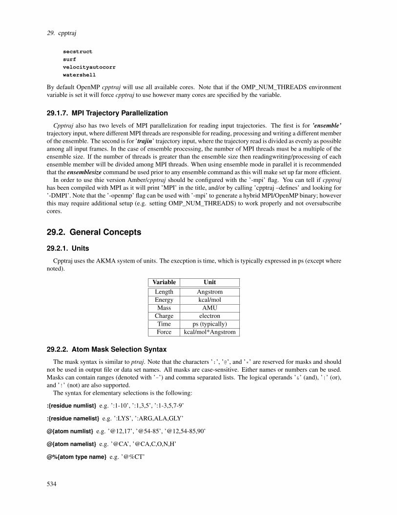
29. cpptraj
secstruct
surf
velocityautocorr
watershell
By default OpenMP cpptraj will use all available cores. Note that if the OMP_NUM_THREADS environmentvariable is set it will force cpptraj to use however many cores are specified by the variable.
29.1.7. MPI Trajectory Parallelization
Cpptraj also has two levels of MPI parallelization for reading input trajectories. The first is for ’ensemble’trajectory input, where different MPI threads are responsible for reading, processing and writing a different memberof the ensemble. The second is for ’trajin’ trajectory input, where the trajectory read is divided as evenly as possibleamong all input frames. In the case of ensemble processing, the number of MPI threads must be a multiple of theensemble size. If the number of threads is greater than the ensemble size then readingwriting/processing of eachensemble member will be divided among MPI threads. When using ensemble mode in parallel it is recommendedthat the ensemblesize command be used prior to any ensemble command as this will make set up far more efficient.
In order to use thie version Amber/cpptraj should be configured with the ’-mpi’ flag. You can tell if cpptrajhas been compiled with MPI as it will print ’MPI’ in the title, and/or by calling ’cpptraj –defines’ and looking for’-DMPI’. Note that the ’-openmp’ flag can be used with ’-mpi’ to generate a hybrid MPI/OpenMP binary; howeverthis may require additional setup (e.g. setting OMP_NUM_THREADS) to work properly and not oversubscribecores.
29.2. General Concepts
29.2.1. Units
Cpptraj uses the AKMA system of units. The execption is time, which is typically expressed in ps (except wherenoted).
Variable UnitLength AngstromEnergy kcal/molMass AMU
Charge electronTime ps (typically)Force kcal/mol*Angstrom
29.2.2. Atom Mask Selection Syntax
The mask syntax is similar to ptraj. Note that the characters ’:’, ’@’, and ’*’ are reserved for masks and shouldnot be used in output file or data set names. All masks are case-sensitive. Either names or numbers can be used.Masks can contain ranges (denoted with ’-’) and comma separated lists. The logical operands ’&’ (and), ’|’ (or),and ’!’ (not) are also supported.
The syntax for elementary selections is the following:
:residue numlist e.g. ’:1-10’, ’:1,3,5’, ’:1-3,5,7-9’
:residue namelist e.g. ’:LYS’, ’:ARG,ALA,GLY’
@atom numlist e.g. ’@12,17’, ’@54-85’, ’@12,54-85,90’
@atom namelist e.g. ’@CA’, ’@CA,C,O,N,H’
@%atom type name e.g. ’@%CT’
534

29.2. General Concepts
@/atom_element_name e.g. ’@/N’
<mask><distance op><distance> Selection by distance, see below.
Several wildcard characters are supported:
’*’ Zero or more characters.
’=’ Same as ’*’
’?’ One character.
The wildcards can also be used with numbers or other mask characters, e.g. ’:?0’ means“:10,20,30,40,50,60,70,80,90”, ’:*’ means all residues and ’@*’ means all atoms.
Compound expressions of the following type are allowed:
:residue numlist | namelist@atom namelist | numlist
and are processed as:
:residue numlist | namelist & @atom namelist | numlist
e.g. ’:1-10@CA’ is equivalent to “:1-10 & @CA”.More examples:
:ALA,TRP All alanine and tryptophan residues.
:5,10@CA CA carbon in residues 5 and 10.
:*&!@H= All non-hydrogen atoms (equivalent to "!@H=").
@CA,C,O,N,H All backbone atoms.
!@CA,C,O,N,H All non-backbone atoms (=sidechains for proteins only).
:1-500@O&!(:WAT|:LYS,ARG) All backbone oxygens in residues 1-500 but not in water, lysine or arginineresidues.
Distance-based Masks
There are two very important things to keep in mind when using distance based masks:
1. Distance-based masks that update each frame are currently only supported by the mask action.
2. Selection by distance for everything but the mask action requires defining a reference frame with reference;distances are then calculated using the specified reference frame only. This reference frame can be changedusing the activeref command.
The syntax for selection by distance is a <mask> expression followed by a <distance operator> followed bya <distance> (which is in Angstroms). The <distance operator> consists of 2 characters: ’<’ (within) or ’>’(without) followed by ’:’ (residues) or ’@’ (atoms), so ’<:’ means “residues within” etc. For residue baseddistance selection, if any atom in that residue matches the given distance criterion, the entire residue is selected.
In plain language, the entire distance mask can be read as “Select <distance operator> <distance> of<mask>”. So for example, the mask expression:
:11-17<@2.4
Means “Select atoms within 2.4 Å distance of atoms selected by ’:11-17’ (residues numbered 11 through 17). Asanother example, to strip everything outside 3.0 Å (i.e. without 3.0 Å) from residue 4 using specified referencecoordinates:
reference mol.rst7
trajin mol.rst7
strip !(:4<:3.0)
535

29. cpptraj
29.2.3. Ranges
For several commands some arguments are ranges (e.g. ’trajout onlyframes <range>’, ’nastruct resrange<range>’, ’rmsd perres range <range>’); THESE ARE NOT ATOM MASKS. They are simple number rangesusing ’-’ to specify a range and ’,’ to separate different ranges. For example 1-2,4-6,9 specifies 1 to 2, 4 to 6, and9, i.e. ’1 2 4 5 6 9’.
29.2.4. Parameter/Reference Tagging
Parameter and reference files may be ’tagged’ (i.e. given a nickname); these tags can then be used in place ofthe file name itself. A tag in cpptraj is recognized by being bounded by brackets (’[’ and ’]’). This can beparticularly useful when reading in many parameter or reference files. For example, when reading in multiplereference structures:
trajin Test1.crd
reference 1LE1.NoWater.Xray.rst7 [xray]
reference Test1.crd lastframe [last]
reference Test2.crd 225 [open]
rms Xray ref [xray] :2-12@CA out rmsd.dat
rms Last ref [last] :2-12@CA out rmsd.dat
rms Open ref [open] :2-12@CA out rmsd.dat
This defines three reference structures and gives them tags [xray], [last], and [open]. These reference structurescan then be referred to by their tags instead of their filenames by any action that uses reference structures (in thiscase the RMSD action).
Similarly, this can be useful when reading in multiple parameter files:
parm tz2.ff99sb.tip3p.truncoct.parm7 [tz2-water]
parm tz2.ff99sb.mbondi2.parm7 [tz2-nowater]
trajin tz2.run1.explicit.nc parm [tz2-water]
reference tz2.dry.rst7 parm [tz2-nowater] [tz2]
rms ref [tz2] !(:WAT) out rmsd.dat
This defines two parm files and gives them tags [tz2-water] and [tz2-nowater], then reads in a trajectory associatedwith one, and a reference structure associated with the other. Note that in the ’reference’ command there are twotags; the first goes along with the ’parm’ keyword and specifies what parameter file the reference should use, thesecond is the tag given to the reference itself (as in the previous example) and is referred to in the subsequentRMSD action.
29.3. Data Sets and Data Files
In cpptraj, Actions and Analyses can generate one or more data sets which are available for further processing.For example, the distance command creates a data set containing distances vs time. The data set can be named bythe user simply by specifying a non-keyword string as an additional argument. If no name is given, a default onewill be generated based on the action name and data set number. For example:
distance d1-2 :1 :2 out d1-2.dat
will create a data set named “d1-2”. If a name is not specified, e.g.:
distance :1 :2 out d1-2.dat
the data set will be named “Dis_00000”.Data files are created automatically by most commands, usually via the “out” keyword. Data files can also
be explicitly created with the write/writedata and create commands. Data can also be read in from files via thereaddata command. Cpptraj currently recognizes the formats listed in 29.1, although it cannot write in all formats.
536
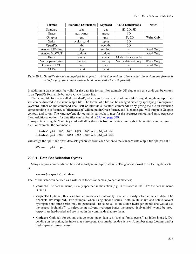
29.3. Data Sets and Data Files
Format Filename Extensions Keyword Valid Dimensions NotesStandard .dat dat 1D, 2D, 3D
Grace .agr, .xmgr grace 1DGnuplot .gnu gnu 1D, 2D Write OnlyXplor .xplor, .grid xplor 3D
OpenDX .dx opendx 3DAmber REM log .log remlog - Read OnlyAmber MDOUT .mdout mdout - Read Only
Evecs .evecs evecs Modes data set onlyVector pseudo-traj .vectraj vectraj Vector data set only. Write Only.
Gromacs XVG .xvg xvg - Read OnlyCCP4 .ccp4 ccp4 3D
Table 29.1.: DataFile formats recognized by cpptraj. ’Valid Dimensions’ shows what dimensions the format isvalid for (e.g. you cannot write a 1D data set with OpenDX format).
In addition, a data set must be valid for the data file format. For example, 3D data (such as a grid) can be writtento an OpenDX format file but not a Grace format file.
The default file format is called ’Standard’, which simply has data in columns, like ptraj, although multiple datasets can be directed to the same output file. The format of a file can be changed either by specifying a recognizedkeyword (either on the command line itself or later via a ’datafile’ command) or by giving the file an extensioncorresponding to te format, so ’filename.agr’ will output in Grace format, and ’filename.gnu’ will output in Gnuplotcontour, and so on. The xmgrace/gnuplot output is particularly nice for the secstruct sumout and rmsd perresoutfiles. Additional options for data files can be found in 29.4 on page 539.
Any action using the “out” keyword will allow data sets from separate commands to be written into the samefile. For example, the commands:
dihedral phi :1@C :2@N :2@CA :2@C out phipsi.dat
dihedral psi :2@N :2@CA :2@C :3@N out phipsi.dat
will assign the “phi” and “psi” data sets generated from each action to the standard data output file “phipsi.dat”:
#Frame phi psi
29.3.1. Data Set Selection Syntax
Many analysis commands can be used to analyze multiple data sets. The general format for selecting data setsis:
<name>[<aspect>]:<index>
The ’*’ character can be used as a wild-card for entire names (no partial matches).
• <name>: The data set name, usually specified in the action (e.g. in ’distance d0 @1 @2’ the data set nameis “d0”).
• <aspect>: Optional; this is set for certain data sets internally in order to easily select subsets of data. Thebrackets are required. For example, when using ’hbond series’, both solute-solute and solute-solventhydrogen bond time series may be generated. To select all solute-solute hydrogen bonds one would usethe aspect “[solutehb]”; to select solute-solvent hydrogen bonds the aspect “[solventhb]” would be used.Aspects are hard-coded and are listed in the commands that use them.
• <index>: Optional; for actions that generate many data sets (such as ’rmsd perres’) an index is used. De-pending on the action, the index may correspond to atom #s, residue #s, etc. A number range (comma and/ordash separated) may be used.
537

29. cpptraj
For example: to select all data sets with aspect “[shear]” named NA_00000:
NA_00000[shear]
To select all data sets with aspect “[stagger]” with any name, indices 1 and 3:
*[stagger]:1,3
In ensemble mode, data set selection has additional syntax:
<name>[<aspect>]:<index>%<member>
Where <member> is the ensemble member number starting from 0.
29.3.2. Data Set Math
As of version 15, cpptraj can perform basic math operations, even on data sets (with some limitations). Currentlyrecognized operations are:
Operation SymbolMinus -Plus +
Divide /Multiply *Power ^Negate -Assign =
Several functions are also supported:
Function FormSquare Root sqrt()Exponential exp()
Natural Logarithm ln()Absolute Value abs()
Sine sin()Cosine cos()Tangent tan()
Summation sum()Average avg()
Standard Deviation stdev()Minimum min()Maximum max()
Numbers can be expressed in scientific notation using “E” notation, e.g. 1E-5 = 0.00001. The parser alsorecognizes PI as the number pi. Expressions can also be enclosed in parentheses. So for example, the followingexpression is valid:
> 1 - ln(sin(PI/4) * 2)^2
Result: 0.879887
Results of numerical calculations like the above can be assigned to a variable (essentially a data set of size 1) foruse in subsequent calculations, e.g.
> R = 1 - ln(sin(PI/4) * 2)^2
Result stored in ’R’
> R + 1 Result: 1.879887
538

29.4. Data File Options
Data sets can be specified in expressions as well. Currently data sets in an expression must be of the same typeand only 1D, 2D, and 3D data sets are supported. Functions are applied to each member of the data set. So forexample, given two 1D data sets of the same size named D0 and D1, the following expression:
> D2 = sqrt( D0 ) + D1
would take the square root of each member of D0, add it to the corresponding member of D1, and assign theresult to D2. The following table lists which operations are valid for data set types. If a type is not listed it is notsupported:
Data Set Type Supported Ops Supported Funcs Notes1D (integer, double, float) All All
1D (vector) +, -, *, /, = None ’*’ is dot product2D (matrices) +, -, /, *, = sum, avg, stdev, min, max
3D (grids) +, -, /, *, = sum, avg, stdev, min, max
29.4. Data File Options
There is a subsection of keywords that can be used to modify data files which have been declared with an ’out’keyword, create new data files from declared data sets, or when reading in data sets from files. Note thatwrite-related keywords can be specified to most actions that use the ’out’ keyword directly without using thedatafile command. For example, the ’time’ argument can be passed directly to the output from a distancecommand:
distance d0 :1 :2 out d0.agr time 0.001
The data file format can be changed from standard implicitly by using specific filename extensions or keywords.If the extension is not recognized or no keyword is give the default format is ’Standard’. Keywords andextensions for data file formats recognized by cpptraj are shown in 29.1. Note that the use of certain options maybe restricted for certain data file formats.
[<format keyword>]
[xlabel|ylabel|zlabel <label>] [xmin|ymin|zmin <min>]
[xstep|ystep|zstep <step>] [time <dt>] [prec <width>[.<precision>]]
xlabel | ylabel | zlabel <label> Set the x-axis label for the specified datafile to
<label>. For regular data files this is the header for the first column of
data. If the data is at least 2-dimensional ’datafile ylabel <label>’ will
likewise set the y-axis label.
xmin | ymin | zmin <min> Set the starting X coordinate value to <min>. If the
data is at least 2-dimensional ’datafile ymin <min>’ will likewise set the
starting Y coordinate value.
xstep | ystep | zstep <step> Multiply each frame number by <step> (x coordinates).
If the data is at least 2-dimensional ’datafile ystep <step>’ will likewise
multiply y coordinates by <step>.
time <dt> Equivalent to the ptraj argument ’time’ that could be specified with
many actions. Multiplies frame numbers (x-axis) by <dt>.
prec <width>[.<precision>] Change the output format width (and optionally
precision) of all sets subsequently added to the data file (i.e. does not
change the precision of any data sets currently in the file). For example,
prec 12.4
prec 10
539
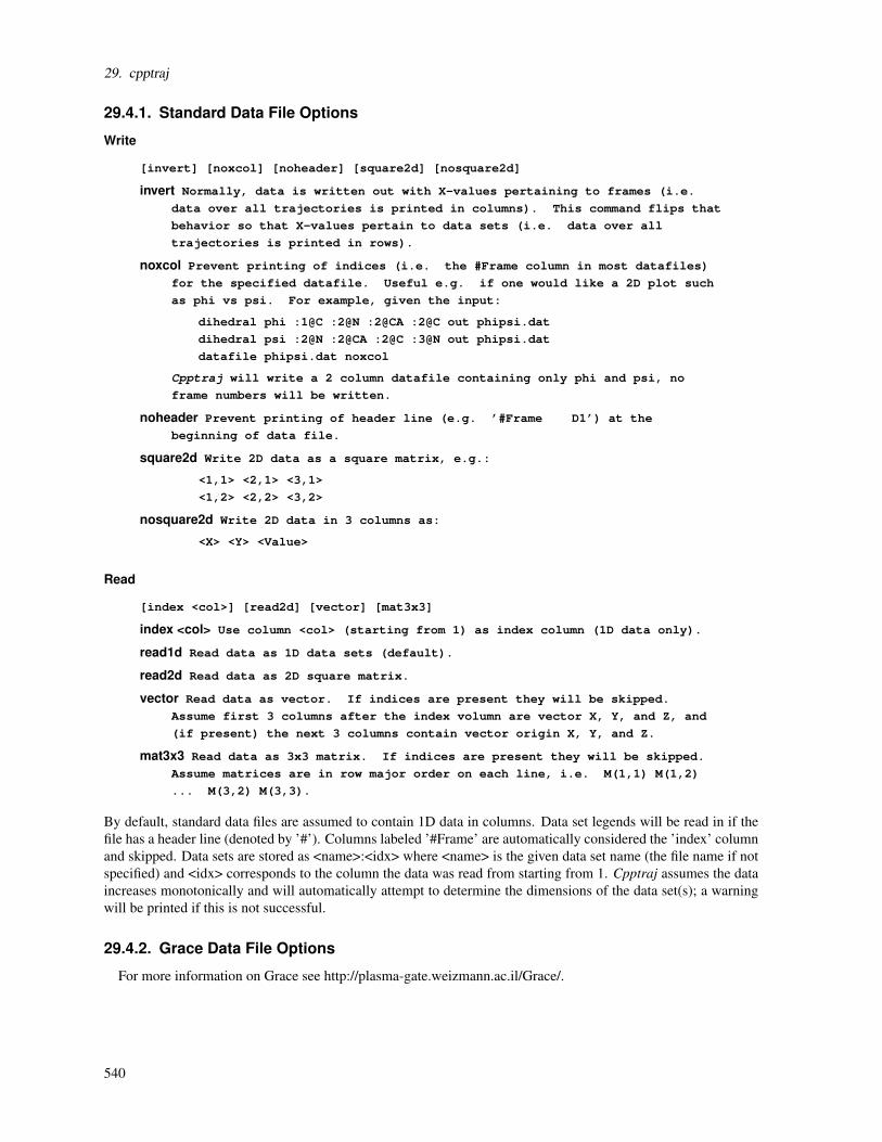
29. cpptraj
29.4.1. Standard Data File Options
Write
[invert] [noxcol] [noheader] [square2d] [nosquare2d]
invert Normally, data is written out with X-values pertaining to frames (i.e.
data over all trajectories is printed in columns). This command flips that
behavior so that X-values pertain to data sets (i.e. data over all
trajectories is printed in rows).
noxcol Prevent printing of indices (i.e. the #Frame column in most datafiles)
for the specified datafile. Useful e.g. if one would like a 2D plot such
as phi vs psi. For example, given the input:
dihedral phi :1@C :2@N :2@CA :2@C out phipsi.dat
dihedral psi :2@N :2@CA :2@C :3@N out phipsi.dat
datafile phipsi.dat noxcol
Cpptraj will write a 2 column datafile containing only phi and psi, no
frame numbers will be written.
noheader Prevent printing of header line (e.g. ’#Frame D1’) at the
beginning of data file.
square2d Write 2D data as a square matrix, e.g.:
<1,1> <2,1> <3,1>
<1,2> <2,2> <3,2>
nosquare2d Write 2D data in 3 columns as:
<X> <Y> <Value>
Read
[index <col>] [read2d] [vector] [mat3x3]
index <col> Use column <col> (starting from 1) as index column (1D data only).
read1d Read data as 1D data sets (default).
read2d Read data as 2D square matrix.
vector Read data as vector. If indices are present they will be skipped.
Assume first 3 columns after the index volumn are vector X, Y, and Z, and
(if present) the next 3 columns contain vector origin X, Y, and Z.
mat3x3 Read data as 3x3 matrix. If indices are present they will be skipped.
Assume matrices are in row major order on each line, i.e. M(1,1) M(1,2)
... M(3,2) M(3,3).
By default, standard data files are assumed to contain 1D data in columns. Data set legends will be read in if thefile has a header line (denoted by ’#’). Columns labeled ’#Frame’ are automatically considered the ’index’ columnand skipped. Data sets are stored as <name>:<idx> where <name> is the given data set name (the file name if notspecified) and <idx> corresponds to the column the data was read from starting from 1. Cpptraj assumes the dataincreases monotonically and will automatically attempt to determine the dimensions of the data set(s); a warningwill be printed if this is not successful.
29.4.2. Grace Data File Options
For more information on Grace see http://plasma-gate.weizmann.ac.il/Grace/.
540

29.4. Data File Options
Write
[invert]
invert Normally, data is written out with X-values pertaining to frames (i.e.
data over all trajectories is printed in columns). This command flips that
behavior so that X-values pertain to data sets.
Read
Cpptraj will read set legends from grace files, and data sets are stored as <name>:<idx> where <name> is thegiven data set name (the file name if not specified) and <idx> corresponds to the set number the data was read fromstarting from 0.
29.4.3. Gnuplot Data File Options
For more information on these options it helps to look at the PM3D options in the Gnuplot manual (seehttp://www.gnuplot.info/).
Write
[nolabels] [usemap] [pm3d] [nopm3d] [jpeg] [noheader]
[xlabels|ylabels|zlabels <labellist>]
nolabels Do not print axis labels.
usemap pm3d output with 1 extra empty row/col (may improve look).
pm3d Normal pm3d map output.
nopm3d Turn off pm3d
jpeg Plot will write to a JPEG file when used with gnuplot.
noheader Do not format plot; data output only.
xlabels|ylabels|zlabels <labellist> Set x, y, or z axis labels with comma-separated
list, e.g. ’xlabels X1,X2,X3’.
29.4.4. Amber REM Log Options
Note that multiple REM logs can be specified in a single readdata command. See 29.10.25 on page 642 formore on replica log analysis.
Read
[nosearch] [dimfile <file>] [crdidx <crd indices>]
[nosearch] If specified do not automatically search for MREMD dimension logs.
[dimfile <file>] remd.dim file for processing MREMD logs.
[crdidx <crd indices>] Use comma-separated list of indices as the initial
coordinate indices (H-REMD only). For example (4 replicas):
crdidx 4,2,3,1
29.4.5. Amber MDOUT Options
Note that multiple MDOUT files can be specified in a single readdata command.
541

29. cpptraj
29.4.6. Evecs File Options
Read
[ibeg <firstmode>] [iend <lastmode>]
ibeg <firstmode> Number of the first mode (or principal component) to read from
evecs file. Default 1.
iend <lastmode> Number of the last mode (or principal component) to read from
evecs file. Default is to read all for newer evecs files (generated by
cpptraj version > 12), 50 for older evecs files.
29.4.7. Vector psuedo-traj Options
This can be used to write out a representation of a vector data set which can then be visualized. See 29.9.78 onpage 616 for more on generating vector data sets.
Write
[trajfmt <format>] [parmout <file>] [noorigin]
trajfmt <format> Output pseudo-trajectory format. See 29.8 on page 557 for
trajectory format keywords.
parmout <file> File to write pseudo-trajectory topology to.
[noorigin] Do not write vector origin coordinates.
29.4.8. OpenDX file options
Write
[bincenter] [gridwrap] [gridext]
bincenter Center grid points on bin centers instead of corners.
gridwrap Like ’bincenter’, but also wrap grid density. Useful when grid
encompasses unit cell.
gridext Like ’bincenter’, but also print extra layer of empty bins.
29.4.9. CCP4 file options
Write
[title <title>]
[title <title>] Set CCP4 output title.
29.5. Coordinates (COORDS) Data Set Commands
Coordinate I/O tends to be the most time-consuming part of trajectory analysis. In addition, many types ofanalyses (for example two-dimensional RMSD and cluster analysis) require using coordinate frames multipletimes. To simplify this, trajectory coordinates may be saved as a separate data set via the loadcrd command orcreatecrd action. Any action can then be performed on the COORDS data set with the crdaction command. Thecrdout command can be used to write coordinates to an output trajectory (similar to trajout).
Although COORDS data sets store everything internally with single-precision, they can still use a large amountof memory. Because of this there is a specialized type of COORDS data set called a TRAJ data set (trajectory),which functions exactly like a COORDS data set except all data is stored on disk. TRAJ data sets can be createdwith the loadtraj command. TRAJ data sets cannot be modified.
542

29.5. Coordinates (COORDS) Data Set Commands
There are several analyses that can be performed using COORDS data sets, either as part of the normal analysislist or via the runanalysis command. Note that while these analyses can be run on specified COORDS data sets, ifone is not specified a default COORDS data set will be created, made up of frames from trajin commands.
As an example of where this might be useful is in the calculation of atomic positional fluctuations. Previouslythis required two steps: one to generate an average structure, then a second to rms-fit to that average structureprior to calculating the fluctuations. This can now be done in one pass with the following input:
parm topology.parm7
loadcrd mdcrd.nc
# Generate average structure PDB, @CA only
crdaction mdcrd.nc average avg.pdb @CA
# Load average structure PDB as reference
parm avg.pdb
reference avg.pdb parm avg.pdb
# RMS-fit to average structure PDB
crdaction mdcrd.nc rms reference @CA
# Calculate atomic fluctuations for @CA only
crdaction mdcrd.nc atomicfluct out fluct.dat bfactor @CA
The following COORDS data set commands are available:
Command Descriptioncombinecrd Combine two or more COORDS sets.
crdaction Run a single Action on a COORDS set.crdout Write a COORDS set to a file.
createcrd (Action) Create a COORDS set during a Run.loadcrd Create or append to a COORDS set from a file.loadtraj Create special COORDS set where frames remain on disk.
reference Load a single trajectory frame as a reference.
29.5.1. combinecrd
combinecrd <crd1> <crd2> ... [parmname <topname>] [crdname <crdname>]
<crdX> COORDS data set to combine, specify 2 or more.
[parmname <topname>] Name of combined Topology.
[crdname <crdname>] Name of combined COORDS data set.
Combined two or more COORDS data sets into a single COORDS data set. Note that the resulting topology willnot be usable for MD simulations. For example, to load two MOL2 files as COORDS data sets, combine them,and write them out as a single MOL2:
loadcrd Tyr.mol2 CRD1
loadcrd Pry.mol2 CRD2
combinedcrd CRD1 CRD2 parmname Parm-1-2 crdname CRD-1-2
crdout CRD-1-2 Tyr.Pry.mol2
29.5.2. crdaction
crdaction <crd set> <actioncmd> [<action args>] [crdframes <start>,<stop>,<offset>]
Perform action <actioncmd> on COORDS data set <crd set>. A subset of frames in the COORDS data set can bespecified with ’crdframes’. For example, to calculate RMSD for a previously created COORDS data set namedcrd1 using frames 1 to the last, skipping every 10:
crdaction crd1 rmsd first @CA out rmsd-ca.agr crdframes 1,last,10
543

29. cpptraj
29.5.3. crdout
crdout <crd set> <filename> [<trajout args>] [crdframes <start>,<stop>,<offset>]
Write COORDS data set <crd set> to trajectory named <filename>. A subset of frames in the COORDS data setcan be specified with ’crdframes’. For example, to write frames 1 to 10 from a previously created COORDS dataset named “crd1” to separate PDB files:
crdout crd1 crd1.pdb multi crdframes 1,10
29.5.4. createcrd
createcrd [<name>] [ parm <name> | parmindex <#> ]
Create a COORDS data set named <name> for frames from trajin commands that are associated with the specifiedtopology.
29.5.5. loadcrd
loadcrd <filename> [parm <parm> | parmindex<#>] [<trajin args>] [name <name>]
Immediately load trajectory <filename> as a COORDS data set named <name> (default base name of<filename>). If <name> is already present the coordinates will be appended to the existing data set. For example,to load frames from trajectories named ’traj1.nc’ and ’traj2.nc’ into a COORDS data set named Crd1:
loadcrd traj1.nc name Crd1
loadcrd traj2.nc name Crd2
29.5.6. loadtraj
loadtraj name <setname> [<filename>]
This command functions in two ways. If <filename> is not provided, all currently loaded input trajectories (fromtrajin commands) are added to TRAJ data set named <setname>. Note that if the input trajectory list is cleared(via ’clear trajin’) this will invalidate the TRAJ data set. In addition, currently all trajectories must have thesame number of atoms. Otherwise add trajectory <filename> to TRAJ data set <setname>.
TRAJ data sets cannot be modifed.
29.5.7. reference
Reference coordinates can now be used and manipulated like COORDS data sets. See 29.8.3 on page 558 forcommand syntax.
29.6. General Commands
The following general commands are available:
544

29.6. General Commands
Command Descriptionactiveref Select the reference for distance-based masks.
clear Clear various objects from the cpptraj state.create Create (but do not yet write) a data file.
datafile Used to manipulate data files.datafilter Filter data sets based on given criteria.dataset Use to manipulate data sets.
debug | prnlev Set debug level. Higher levels give more info.exit | quit Quit cpptraj.go | run Start a trajectory processing Run.
help Provide help for commands.list List various objects in the cpptraj state.
noexitonerror Attempt to continue even if errors are encountered.noprogress Do not print a progress bar during a Run.
permutedihedrals Rotate dihedrals in a COORDS set randomly or by intervals.precision Change the output precision of data sets.printdata Print data set to screen.readdata Read data sets from files.readinput Read cpptraj input from a file.
removedata Remove specified data set(s).rst Generate Amber-style distance/angle/torsion restraints.
runanalysis Run an analysis immediately or run all queued analyses.select Print the results of an atom mask expression.
selectds Print the results of a data set selection expression.silenceactions Prevent Actions from writing information to STDOUT.
write | writedata Immediately write data to a file or write to all current data files.
29.6.1. activeref
activeref <#>
Set which reference structure should be used when setting up distance-based masks for everything but the ’mask’action. Numbering starts from 0, so ’activeref 0’ selects the first reference structure read in, ’activeref 1’ selectsthe second, and so on.
29.6.2. clear
clear [all | <type>]
(<type> = actions,trajin,trajout,ref,parm,analysis,datafile,dataset)
Clear list of indicated type, or all lists if ’all’ specified. Note that when clearing actions or analyses, associateddata sets and data files are not cleared and vice versa.
29.6.3. create
create <filename> <datasetname0> [<datasetname1> ...] [<DataFile Options>]
Add specified data sets to the data file named <filename>; if the file does not exist, it will be added to theDataFileList. Data files created in this way are only written at the end of coordinate processing, analyses, orvia the ’writedata’ command. See 29.4 on page 539 for more data file format options.
545

29. cpptraj
29.6.4. datafile
datafile <filename> <datafile arg>
Pass <datafile arg> to data file <filename>. See 29.4 on page 539 for more details.
29.6.5. datafilter
datafilter <dataset arg> min <min> max <max> [out <file> [name <setname>]]
<dataset arg> min <min> max <max> Data set and min/max cutoffs to use; can
specify more than once.
[out <file>] Write out to file named <file>.
[name <setname>] Name of filter data set.
Create a data set (optionally named <setname>) containing 1 for data within given <min> and <max> criteria foreach specified data set. There must be at least one <min> and <max> argument, and can be as many as there arespecified data sets. For example, to read in data from two separate files (d1.dat and a1.dat) and generate a filterdata set named FILTER having 1 when d1 is between 0.0 and 3.0 and a1 is between 135.0 and 180.0:
readdata a1.dat name a1
readdata d1.dat name d1
datafilter d1 min 0.0 max 3.0 a1 min 135.0 max 180.0 out filter.dat name FILTER
Note that a similar command that can be used with data generated by Actions during trajectory processing is filter(see page 579).
29.6.6. dataset
dataset legend <legend> <set> |
makexy <Xset> <Yset> [name <name>] |
cat <set0> <set1> ... [name <name>] [nooffset] |
[mode <mode>] [type <type>] <set arg1> [<set arg 2> ...]
<mode>: distance angle torsion pucker rms
<type>: alpha beta gamma delta epsilon zeta pucker chi h1p c2p
phi psi pchi omega noe
Options for ’type noe’:
[bound <lower> bound <upper>] [rexp <expected>] [noe_strong] [noe_medium] [noe_weak]
legend <legend> <set> Set the legend for data set <set>.
[name <name>] New data set name for makexy/cat.
makexy <Xset> <Yset> Create a new data set (optionally named <name>) with X
values from <Xset> and Y values from <Yset>.
cat <set0> <set1> ... Concatenate two or more data sets into a new data set
(optionally named <name>).
[mode <mode>] Set data set(s) mode to <mode>.
[type <type>] Set data set(s) type to ’type’, useful for e.g. analysis with
statistics. Note this can also be done with ’type <type>’ for certain
commands (distance, dihedral, pucker etc). Note that not every <type> is
compatible with a given <mode>.
Options for type noe only:
[bound <lower> bound <upper>] Lower and upper bounds for NOE (in Angstroms); must
specify both.
546

29.6. General Commands
[rexp <expected>] Expected value for NOE (in Angstroms); if not given ’(<lower> +
<upper>)’ / 2.0 is used.
[noe_strong] Set lower and upper bounds to 1.8 and 2.9 Å respectively.
[noe_medium] Set lower and upper bounds to 2.9 and 3.5 Å respectively.
[noe_weak] Set lower and upper bounds to 3.5 and 5.0 Å respectively.
Either set the legend for a single data set, create a new set with X values from one set and Y values from another,concatenate 2 or more sets, or change the mode/type for one or more data sets. Setting the mode/type can be usefulfor cases where the data set is being read in from a file; for example when reading in a dihedral data set the type canbe set to ’dihedral’ so that various Analysis routines like statistics know to treat it as periodic. A brief descriptionof possible modes and types follows:
Mode Type Descriptiondistance noe NOE distance.
angle Angle.torsion alpha Nucleic acid alpha.
beta Nucleic acid beta.gamma Nucleic acid gamma.delta Nucleic acid delta.
epsilon Nucleic acid epsilon.zeta Nucleic acid zeta.nu1 Nucleic pucker (O4’).nu2 Nucleic pucker (C4’).h1p Nucleic acid H1’.c2p Nucleic acid C2’.chin Nucleic acid chi.phi Protein Phi.psi Protein psi.
chip Protein chi.omega Protein omega.
pucker pucker Sugar pucker.rms RMSD.
matrix distance Distance matrix.covariance Cartesian covariance matrix.
’mass-weighted covariance’ Mass weighted Cartesian covariance matrix.correlation Dynamic cross correlation matrix.
’distance covariance’ Distance covariance matrix.IDEA IDEA matrix.IRED IRED matrix.
’dihedral covariance’ Dihedral covariance matrix.vector IRED IRED vector.
29.6.7. debug | prnlev
debug [<type>] <#>
(<type> = actions,trajin,trajout,ref,parm,analysis,datafile,dataset)
Set the level of debug information to print. In general the higher the <#> the more information that is printed. If<type> is specified only set the debug level for a specific area of cpptraj.
29.6.8. exit | quit
Exit normally.
547

29. cpptraj
29.6.9. go | run
Begin trajectory processing, followed by analysis and datafile write.
29.6.10. help
help [<command>] | General | Action | Analysis | Topology | Trajectory
By itself, list all commands known to cpptraj. If given with a command, print help for that command. Otherwise,list all commands of a certain category (General, Action, Analysis, Topology, or Trajectory).
29.6.11. list
list <type>
(<type> = actions,trajin,trajout,ref,parm,analysis,datafile,dataset)
List the currently loaded objects of <type>.
29.6.12. noexitonerror
noexitonerror
Normally cpptraj will exit if actions fail to initialize properly. If noexitonerror is specified, cpptraj will attempt tocontinue past such errors. This is the default if in interactive mode.
29.6.13. noprogress
noprogress
Do not display read progress during trajectory processing.
29.6.14. permutedihedrals
permutedihedrals crdset <COORDS set> resrange <range> [interval | random]
[outtraj <filename> [<outfmt>]] [crdout <output COORDS>] [<dihedral types>]
Options for ’random’:
[rseed <rseed>] [out <# problems file> [<set name>]]
[ check [cutoff <cutoff>] [rescutoff <rescutoff>] [checkallresidues]
[backtrack <backtrack>] [increment <increment>] [maxfactor <max_factor>] ]
Options for ’interval’:
<interval deg>
<dihedral types> = alpha beta gamma delta epsilon zeta nu1 nu2 h1p c2p chin phi psi chip omega
crdset <COORDS set> COORDS data set to operate on.
resrange <range> Residue range to search for dihedrals.
interval Rotate found dihedrals by <interval>. This is done in an ordered
fashion so that every combination of dihedral rotations is sampled at least
once.
random Rotate each found dihedral randomly.
[outtraj <filename>] Trajectory file to write coordinates to.
[<outfmt>] Trajectory file format.
[crdout <output COORDS>] COORDS data set to write coordinates to.
<dihedral type> One or more dihedral types to search for.
548

29.6. General Commands
Options for ’interval:
<interval deg> Amount to rotate dihedral by each step.
Options for ’random’:
[rseed <rseed>] Random number seed.
[out <# problems file>] File to write number of problems (clashes) each frame to.
[<set name>] Number of problems data set name.
[check] Check randomly rotated structure for clashes.
[cutoff <cutoff>] Atom cutoff for checking for clashes (default 0.8 Å).
[rescutoff <cutoff>] Residue cutoff for checking for clashes (defualt 10.0 Å).
[checkallresidues] If specified all residues checked for clashes, otherwise
only residues up to the currently rotated dihedral check.
[backtrack <backtrack>] If a clash is encountered at dihedral N and cannot be
resolved, go to dihedral N-<backtrack> to try and resolve the clash
(default 4).
[increment <increment>] If a clash is encountered, first attempt to rotate
dihedral by increment to resolve it; if it cannot be resolved by a full
rotation the calculation will backtrack (default 1).
[maxfactor <max_factor>] The maximum number of total attempted rotations will
be <max_factor> * <total # of dihedrals> (default 2).
Create a trajectory by rotating specified dihedrals in a structure by regular intervals (interval), or create 1 structureby randomly rotating specified dihedrals (random). When randomly rotating dihedrals steric clashes will bechecked if check is specified; in such cases the algorithm will attempt to resolve the clash as best it can. Ifclashes are not being resolved you can increase the number of rotation attempts cpptraj will make by increasingmaxfactor.
For example, to rotate all backbone dihedrals in a protein with coordinates in a file named tz2.rst7 in -120degree intervals and write the resulting trajectory in Amber format to rotations.mdcrd:
reference tz2.rst7 [TZ2]
permutedihedrals crdset [TZ2] interval -120 outtraj rotations.mdcrd phi psi
To randomly rotate backbone dihedrals for the same structure and write to file random.mol2 in MOL2 format:
reference tz2.rst7 [TZ2]
permutedihedrals crdset [TZ2] random rseed 1 check maxfactor 10 phi psi \
outtraj random.mol2 multi
29.6.15. precision
precision <filename> | <dataset arg> [<width>] [<precision>]
Set the precision for all data sets in data file <filename> or data set(s) specified by <dataset arg> to width.precision,where width is the column width and precision is the number of digits after the decimal point. Note that the<precision> argument only applies to floating-point data sets.
For example, if one wanted to set the precision of the output of an Rmsd calculation to 8.3, the input could be:
trajin ../run0.nc
rms first :10-260 out prec.dat
precision prec.dat 8 3
and the output would look like:
#Frame RMSD_00000
1 0.000
2 0.630
549
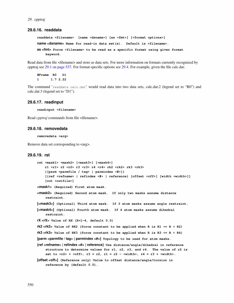
29. cpptraj
29.6.16. readdata
readdata <filename> [name <dsname>] [as <fmt>] [<format options>]
name <dsname> Name for read-in data set(s). Default is <filename>.
as <fmt> Force <filename> to be read as a specific format using given format
keyword.
Read data from file <filename> and store as data sets. For more information on formats currently recognized bycpptraj see 29.1 on page 537. For format-specific options see 29.4. For example, given the file calc.dat:
#Frame R0 D1
1 1.7 2.22
The command ’readdata calc.dat’ would read data into two data sets, calc.dat:2 (legend set to “R0”) andcalc.dat:3 (legend set to “D1”).
29.6.17. readinput
readinput <filename>
Read cpptraj commands from file <filename>.
29.6.18. removedata
removedata <arg>
Remove data set corresponding to <arg>.
29.6.19. rst
rst <mask1> <mask2> [<mask3>] [<mask4>]
r1 <r1> r2 <r2> r3 <r3> r4 <r4> rk2 <rk2> rk3 <rk3>
[parm <parmfile / tag> | parmindex <#>]
[ref <refname> | refindex <#> | reference [offset <off>] [width <width>]]
[out <outfile>]
<mask1> (Required) First atom mask.
<mask2> (Required) Second atom mask. If only two masks assume distance
restraint.
[<mask3>] (Optional) Third atom mask. If 3 atom masks assume angle restraint.
[<mask4>] (Optional) Fourth atom mask. If 4 atom masks assume dihedral
restraint.
rX <rX> Value of RX (X=1-4, default 0.0)
rk2 <rk2> Value of RK2 (force constant to be applied when R is R1 <= R < R2)
rk3 <rk3> Value of RK3 (force constant to be applied when R is R3 <= R < R4)
[parm <parmfile / tag> | parmindex <#>] Topology to be used for atom masks.
ref <refname> | refindex <#> | reference Use distance/angle/dihedral in reference
structure to determine values for r1, r2, r3, and r4. The value of r2 is
set to <r2> + <off>, r3 = r2, r1 = r2 - <width>, r4 = r3 + <width>.
[offset <off>] (Reference only) Value to offset distance/angle/torsion in
reference by (default 0.0).
550

29.6. General Commands
[width <width>] (Reference only) Width between r1 and r2, r3 and r4 (default
0.5).
[out <outfile>] Write restraints to outfile. If not specified, write to STDOUT.
Generate Amber-style distance restraints for use with nmropt=1. This is particularly useful for generatingdistance restraints based off of reference coordinates. For example to generate a distance restraint between twoC5’ atoms using the current distance between them in a reference structure, offsetting the distance by 1.0 Ang.:
parm 30bp-longbox-tip3p-na.parm7
reference 30bp-longbox.rst7
rst :1@C5’ :31@C5’ reference offset 1.0 rk2 10.0 rk3 10.0 out output
29.6.20. runanalysis
runanalysis [<analysiscmd> [<analysis args>]]
Run given analysis command immediately and write any data generated. If no command is given run any analysiscurrently set up. NOTE: When ’runanalysis’ is specified alone, data is not automatically written; to write datagenerated with ’runanalysis’ use the ’writedata’ command (this allows multiple analysis runs between output ifdesired).
29.6.21. select
select <mask>
Prints the number of selected atoms corresponding to the given mask, as well as the atom numbers with format:
Selected= <#atom1> <#atom2> ...
This does not affect the state in any way, but is intended for use in scripts etc. for testing the results of a maskexpression.
29.6.22. selectds
selectds <dataset arg>
Show the results of a data set selection. Data set selection has the format:
<name>[<aspect>]:<index>
Either the [<aspect>] or the <index> arguments may be omitted. A ’*’ can be used in place of <name> or [<as-pect>] as a wildcard. The <index> argument can be a single number or a range separated by ’-’ and ’,’.
This command does not affect the state in any way, but is particularly useful in interactive mode for determiningthe results of a dataset argument.
29.6.23. write | writedata
write [<filename> <datasetname0> [<datasetname1> ...]] [<DataFile Options>]
With no arguments, write all files currently in the data file list. Otherwise, write specified data set(s) to <filename>.This is like the ’create’ command except a data file is not added to the data file list; it is written immediately.See 29.4 on page 539 for more data file format options.
551
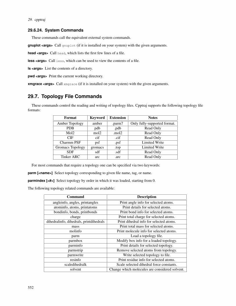
29. cpptraj
29.6.24. System Commands
These commands call the equivalent external system commands.
gnuplot <args> Call gnuplot (if it is installed on your system) with the given arguments.
head <args> Call head, which lists the first few lines of a file.
less <args> Call less, which can be used to view the contents of a file.
ls <args> List the contents of a directory.
pwd <args> Print the current working directory.
xmgrace <args> Call xmgrace (if it is installed on your system) with the given arguments.
29.7. Topology File Commands
These commands control the reading and writing of topology files. Cpptraj supports the following topology fileformats:
Format Keyword Extension NotesAmber Topology amber .parm7 Only fully-supported format.
PDB pdb .pdb Read OnlyMol2 mol2 .mol2 Read OnlyCIF cif .cif Read Only
Charmm PSF psf .psf Limited WriteGromacs Topology gromacs .top Limited Write
SDF sdf .sdf Read OnlyTinker ARC arc .arc Read Only
For most commands that require a topology one can be specified via two keywords:
parm [<name>] Select topology corresponding to given file name, tag, or name.
parmindex [<#>] Select topology by order in which it was loaded, starting from 0.
The following topology related commands are available:
Command Descriptionangleinfo, angles, printangles Print angle info for selected atoms.atominfo, atoms, printatoms Print details for selected atoms.bondinfo, bonds, printbonds Print bond info for selected atoms.
charge Print total charge for selected atoms.dihedralinfo, dihedrals, printdihedrals Print dihedral info for selected atoms.
mass Print total mass for selected atoms.molinfo Print molecule info for selected atoms.
parm Load a topology file.parmbox Modify box info for a loaded topology.parminfo Print details for selected topology.parmstrip Remove selected atoms from topology.parmwrite Write selected topology to file.
resinfo Print residue info for selected atoms.scaledihedralk Scale selected dihedral force constants.
solvent Change which molecules are considered solvent.
552

29.7. Topology File Commands
29.7.1. angleinfo | angles | printangles
angleinfo [parm <name> | parmindex <#> | <#>] [<mask>]
Print angle information of atoms in <mask> for selected topology (first loaded topology by default) with format:
# Angle Kthet degrees atom names (numbers)
Where Angle is the internal angle index, Kthet is the angle force constant, degrees is the angle equilibrium value,atom names shows the atoms involved in the angle with format :<residue num>@<atom name>, and (numbers)
shows the atom indices involved in a comma-separated list. Atom types will be shown in the last column.
29.7.2. atominfo | atoms | printatoms
atominfo [parm <name> | parmindex <#> | <#>] [<mask>]
Print information on atoms in <mask> for selected topology (first loaded topology by default) with format:
#Atom Name #Res Name #Mol Type Charge Mass GBradius El [rVDW] [eVDW]
where #Atom is the internal atom index, the first Name column is the atom name, #Res is the atom’s residue number,the second Name column is residue name, #Mol is the atom’s molecule number, Type is the atom’s type (certaintopologies only), Charge is the atom charge (in units of electron charge), Mass is the atom’s mass (in amu),GBradius is the generalized Born radius of the atom (Amber topologies only), and El is the 2 character elementstring. The final two columns are only shown if the topology contains non-bonded parameters: rVDW is the atom’sLennard-Jones radius and eVDW is the atom’s Lennard-Jones epsilon.
29.7.3. bondinfo | bonds | printbonds
bondinfo [parm <name> | parmindex <#> | <#>] [<mask>]
Print bond information for atoms in <mask> for selected topology (first loaded topology by default) with format:
# Bond Kb Req atom names (numbers)
where Bond is the internal bond index, Kb is the bond force constant, Req is the bond equilibrium value (inAngstroms), atom names shows both atom names with format :<residue num>@<atom name>, and (numbers)
shows both atom numbers in a comma-separated list. Atom types will be shown in the last column.
29.7.4. charge
charge [parm <name> | parmindex <#> | <#>] <mask>
Print the total charge of atoms in <mask> (in units of electron charge) for selected topology (first loaded topologyby default).
29.7.5. dihedralinfo | dihedrals | printdihedrals
dihedralinfo [parm <name> | parmindex <#> | <#>] [<mask>] [and]
Print dihedral information of atoms in <mask> for selected topology (first loaded topology by default) withformat:
#Dihedral pk phase pn atoms
553
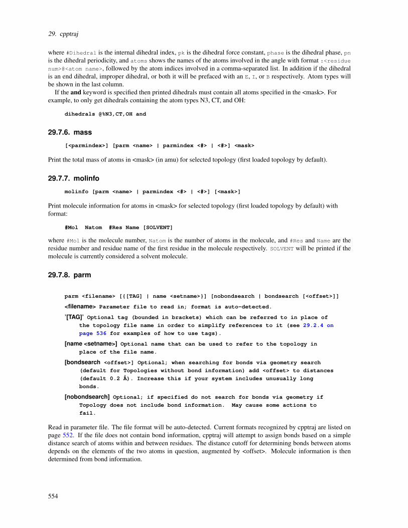
29. cpptraj
where #Dihedral is the internal dihedral index, pk is the dihedral force constant, phase is the dihedral phase, pnis the dihedral periodicity, and atoms shows the names of the atoms involved in the angle with format :<residuenum>@<atom name>, followed by the atom indices involved in a comma-separated list. In addition if the dihedralis an end dihedral, improper dihedral, or both it will be prefaced with an E, I, or B respectively. Atom types willbe shown in the last column.
If the and keyword is specified then printed dihedrals must contain all atoms specified in the <mask>. Forexample, to only get dihedrals containing the atom types N3, CT, and OH:
dihedrals @%N3,CT,OH and
29.7.6. mass
[<parmindex>] [parm <name> | parmindex <#> | <#>] <mask>
Print the total mass of atoms in <mask> (in amu) for selected topology (first loaded topology by default).
29.7.7. molinfo
molinfo [parm <name> | parmindex <#> | <#>] [<mask>]
Print molecule information for atoms in <mask> for selected topology (first loaded topology by default) withformat:
#Mol Natom #Res Name [SOLVENT]
where #Mol is the molecule number, Natom is the number of atoms in the molecule, and #Res and Name are theresidue number and residue name of the first residue in the molecule respectively. SOLVENT will be printed if themolecule is currently considered a solvent molecule.
29.7.8. parm
parm <filename> [[TAG] | name <setname>] [nobondsearch | bondsearch [<offset>]]
<filename> Parameter file to read in; format is auto-detected.
’[TAG]’ Optional tag (bounded in brackets) which can be referred to in place of
the topology file name in order to simplify references to it (see 29.2.4 on
page 536 for examples of how to use tags).
[name <setname>] Optional name that can be used to refer to the topology in
place of the file name.
[bondsearch <offset>] Optional; when searching for bonds via geometry search
(default for Topologies without bond information) add <offset> to distances
(default 0.2 Å). Increase this if your system includes unusually long
bonds.
[nobondsearch] Optional; if specified do not search for bonds via geometry if
Topology does not include bond information. May cause some actions to
fail.
Read in parameter file. The file format will be auto-detected. Current formats recognized by cpptraj are listed onpage 552. If the file does not contain bond information, cpptraj will attempt to assign bonds based on a simpledistance search of atoms within and between residues. The distance cutoff for determining bonds between atomsdepends on the elements of the two atoms in question, augmented by <offset>. Molecule information is thendetermined from bond information.
554

29.7. Topology File Commands
29.7.8.1. PDB format:
[pqr] [readbox] [noconect]
[pqr]: Read charge and radius information from the occupancy and B-factor
columns.
[readbox]: Read unit cell information from CRYST1 record if present.
[noconect] Do not read in CONECT records from PDB file.
IMPORTANT NOTES FOR PDB FILES
In some older format PDB files (before version 3), certain atoms may contain the asterisk (’*’) character in theirname (e.g. ’C1*’ in a nucleic acid backbone). Since in cpptraj the asterisk is a reserved character for atom masksall asterisks in PDB atom names are replaced with single quote (’) to avoid issues with the mask parser. So in astructure with an atom named C1*, to select it use the mask “@C1”’.
Sometimes PDB files can contain alternate coordinates for the same atom in a residue, e.g.:
ATOM 806 CA ACYS A 105 6.460 -34.012 -21.801 0.49 32.23
ATOM 807 CB ACYS A 105 6.054 -33.502 -20.415 0.49 35.28
ATOM 808 CA BCYS A 105 6.468 -34.015 -21.815 0.51 32.42
ATOM 809 CB BCYS A 105 6.025 -33.499 -20.452 0.51 35.38
If this is the case cpptraj will print a warning about duplicate atom names but will take no other action. Bothresidues are considered ’CYS’ and the mask ’:CYS@CA’ would select both atom 806 and 809. Residue insertioncodes are read in but also not used by the mask parser.
29.7.9. parmbox
parmbox [parm <name> | parmindex <#> | <#>] [nobox] [truncoct]
[x <xval>] [y <yval>] [z <zval>] [alpha <a>] [beta <b>] [gamma <g>]
[parm <name> | parmindex <#> | <#>] Name/tag or index of topology to modify.
Default is first loaded topology.
[nobox] Remove box information.
[truncoct] Set truncated octahedon angles with lengths equal to <xval>.
[x <xval>] Box X length.
[y <yval>] Box Y length.
[z <zval>] Box Z length.
[alpha <a>] Box alpha angle.
[beta <b>] Box beta angle.
[gamma <g>] Box gamma angle.
Modify the box information for specified topology. Overwrites any box information if present with specifiedvalues; any that are not specified will remain unchanged. Note that unlike the box action this command affect boxinformation immediately. This can be useful for e.g. removing box information from a parm when strippingsolvent:
parm mol.water.parm7
parmstrip :WAT
parmbox nobox
parmwrite out strip.mol.nobox.parm7
555
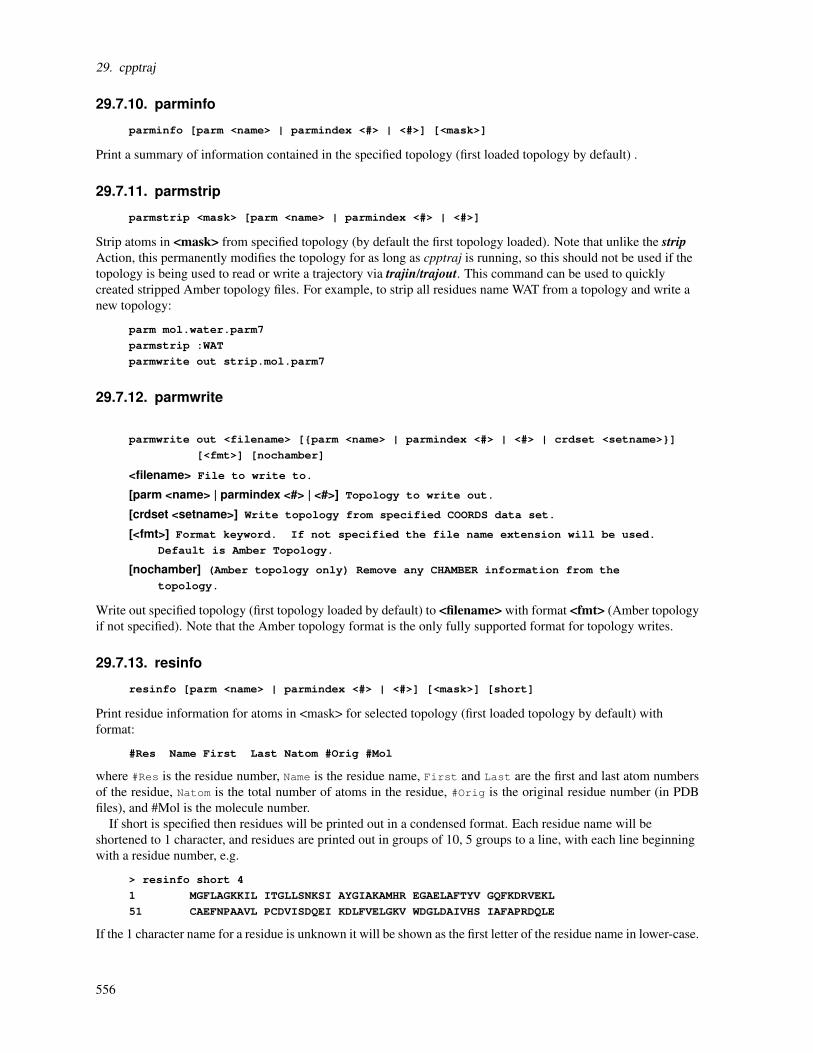
29. cpptraj
29.7.10. parminfo
parminfo [parm <name> | parmindex <#> | <#>] [<mask>]
Print a summary of information contained in the specified topology (first loaded topology by default) .
29.7.11. parmstrip
parmstrip <mask> [parm <name> | parmindex <#> | <#>]
Strip atoms in <mask> from specified topology (by default the first topology loaded). Note that unlike the stripAction, this permanently modifies the topology for as long as cpptraj is running, so this should not be used if thetopology is being used to read or write a trajectory via trajin/trajout. This command can be used to quicklycreated stripped Amber topology files. For example, to strip all residues name WAT from a topology and write anew topology:
parm mol.water.parm7
parmstrip :WAT
parmwrite out strip.mol.parm7
29.7.12. parmwrite
parmwrite out <filename> [parm <name> | parmindex <#> | <#> | crdset <setname>]
[<fmt>] [nochamber]
<filename> File to write to.
[parm <name> | parmindex <#> | <#>] Topology to write out.
[crdset <setname>] Write topology from specified COORDS data set.
[<fmt>] Format keyword. If not specified the file name extension will be used.
Default is Amber Topology.
[nochamber] (Amber topology only) Remove any CHAMBER information from the
topology.
Write out specified topology (first topology loaded by default) to <filename> with format <fmt> (Amber topologyif not specified). Note that the Amber topology format is the only fully supported format for topology writes.
29.7.13. resinfo
resinfo [parm <name> | parmindex <#> | <#>] [<mask>] [short]
Print residue information for atoms in <mask> for selected topology (first loaded topology by default) withformat:
#Res Name First Last Natom #Orig #Mol
where #Res is the residue number, Name is the residue name, First and Last are the first and last atom numbersof the residue, Natom is the total number of atoms in the residue, #Orig is the original residue number (in PDBfiles), and #Mol is the molecule number.
If short is specified then residues will be printed out in a condensed format. Each residue name will beshortened to 1 character, and residues are printed out in groups of 10, 5 groups to a line, with each line beginningwith a residue number, e.g.
> resinfo short 4
1 MGFLAGKKIL ITGLLSNKSI AYGIAKAMHR EGAELAFTYV GQFKDRVEKL
51 CAEFNPAAVL PCDVISDQEI KDLFVELGKV WDGLDAIVHS IAFAPRDQLE
If the 1 character name for a residue is unknown it will be shown as the first letter of the residue name in lower-case.
556
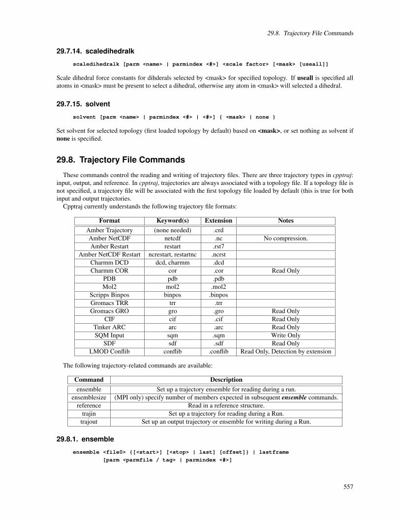
29.8. Trajectory File Commands
29.7.14. scaledihedralk
scaledihedralk [parm <name> | parmindex <#>] <scale factor> [<mask> [useall]]
Scale dihedral force constants for dihderals selected by <mask> for specified topology. If useall is specified allatoms in <mask> must be present to select a dihedral, otherwise any atom in <mask> will selected a dihedral.
29.7.15. solvent
solvent [parm <name> | parmindex <#> | <#>] <mask> | none
Set solvent for selected topology (first loaded topology by default) based on <mask>, or set nothing as solvent ifnone is specified.
29.8. Trajectory File Commands
These commands control the reading and writing of trajectory files. There are three trajectory types in cpptraj:input, output, and reference. In cpptraj, trajectories are always associated with a topology file. If a topology file isnot specified, a trajectory file will be associated with the first topology file loaded by default (this is true for bothinput and output trajectories.
Cpptraj currently understands the following trajectory file formats:
Format Keyword(s) Extension NotesAmber Trajectory (none needed) .crdAmber NetCDF netcdf .nc No compression.Amber Restart restart .rst7
Amber NetCDF Restart ncrestart, restartnc .ncrstCharmm DCD dcd, charmm .dcdCharmm COR cor .cor Read Only
PDB pdb .pdbMol2 mol2 .mol2
Scripps Binpos binpos .binposGromacs TRR trr .trrGromacs GRO gro .gro Read Only
CIF cif .cif Read OnlyTinker ARC arc .arc Read OnlySQM Input sqm .sqm Write Only
SDF sdf .sdf Read OnlyLMOD Conflib conflib .conflib Read Only, Detection by extension
The following trajectory-related commands are available:
Command Descriptionensemble Set up a trajectory ensemble for reading during a run.
ensemblesize (MPI only) specify number of members expected in subsequent ensemble commands.reference Read in a reference structure.
trajin Set up a trajectory for reading during a Run.trajout Set up an output trajectory or ensemble for writing during a Run.
29.8.1. ensemble
ensemble <file0> [<start>] [<stop> | last] [offset] | lastframe
[parm <parmfile / tag> | parmindex <#>]
557

29. cpptraj
[trajnames <file1>,<file2>,...,<fileN>
[remlog <remlogfile> [nstlim <nstlim> ntwx <ntwx>]]
<file0> Lowest replica filename.
[<start>] Frame to begin reading ensemble at (default 1).
[<stop> | last] Frame to stop reading ensemble at; if not specified or ’last’
specified, end of trajectories.
[<offset>] Offset for reading in trajectory frames (default 1).
[lastframe] Select only the final frame of the trajectories.
[parm <parmfile>] Topology filename/tag to associate with trajectories (default
first topology).
[parmindex <#>] Index of Topology to associate with trajectories (default 0,
first topology).
[trajnames <file1>,...,<fileN>] Do not automatically search for additional replica
trajectories; use comma-separated list of trajectory names.
[remlog <remlogfile>] For H-REMD trajectories only, use specified REMD log file to
sort trajectories by coordinate index (instead of by Hamiltonian).
[nstlim <nstlim> ntwx <ntwx>] If trajectory and REMD log were not written at
the same rate, these are the values for nstlim (steps between each
exchange) and ntwx (steps between trajectory write) used in the REMD
simulation.
Read in and process trajectories as an ensemble. Similar to ’trajin remdtraj’, except instead of processing oneframe at a target temperature, process all frames. This means that action and trajout commands apply to the entireensemble; note however that not all actions currently function in ’ensemble’ mode. For example, to read in areplica ensemble, convert it to temperature trajectories, and calculate a distance at each temperature:
parm ala2.99sb.mbondi2.parm7
ensemble rem.crd.000 trajnames rem.crd.001,rem.crd.002,rem.crd.003
trajout temp.crd
distance d1 out d1.ensemble.dat @1 @21
This will output 4 temperature trajectories named ’temp.crd.X’, where X ranges from 0 to 3 with 0 correspondingto the lowest temperature, and ’d1.ensemble.dat’ containing 4 columns, each corresponding to a temperature. Ifrun with MPI, data will be written to separate files named ’d1.ensemble.dat.X’, similar to the output trajectories.
Note that in parallel (i.e. MPI) users should specify the ensemblesize command prior to ensemble in order toimprove set up efficiency.
29.8.2. ensemblesize
ensemblesize <#>
This command is MPI only. It is used to set the expected number of members in any subsequent ensemble com-mand, which dramatically improves set up efficiency.
29.8.3. reference
reference <name> [<frame#>] [<mask>] ([tag]) [lastframe] [crdset]
[parm <parmfile / tag> | parmindex <#>]
<name> File name (or COORDS set name if ’crdset’ specified) to read in as
reference; any trajectory recognized by ’trajin’ can be used.
558

29.8. Trajectory File Commands
[<frame#>] Frame number to use (default 1).
[<mask>] Only load atoms corresponding to <mask> from reference.
([tag]) Tag to give this reference file, e.g. “[MyRef]”; BRACKETS MUST BE
INCLUDED.
[lastframe] Use last frame of reference.
[crdset] Use for COORDS data set named <name> instead of file.
[parm <parmfile/tag>] Topology filename/tag to associate with reference (default
first topology).
[parmindex <#>] Index of Topology to associate with reference (default 0, first
topology).
Use specified trajectory as reference coordinates. For trajectories with multiple frames, the first frame is used if aspecific frame is not specified. An optional tag can be given (bounded in brackets) which can then be used in placeof the name (see 29.2.4 on page 536 for examples of how to use tags). If desired, an atom mask can be used toread in only specified atoms from a reference.
Reference coordinates are now considered COORDS data sets and can be used anywhere a COORDS data setcould, which allows reference structures to be manipulated once they are loaded. For example, a referencestructure could be centered on the origin like so:
reference tz2.rst7 [MyRef]
crdaction [MyRef] center origin
Note that the ’average’ keyword has been deprecated for reference. If desired, an averaged reference COORDSdata set can be created from a trajectory using the ’average’ command like so:
parm myparm.parm7
trajin mytraj.nc
rms first :1-12
average crdset RefAvg
run
rms ToAvg reference :1-12 out ToAvg.dat
29.8.4. trajin
trajin <filename> [<start> [<stop> | last] [<offset>]] | lastframe
[parm <parmfile / tag> | parmindex <#>]
[ <Format Options> ]
[ remdtraj remdtrajtemp <Temperature> | remdtrajidx <#>
[trajnames <file1>,<file2>,...,<fileN>] ]
<filename> Trajectory file to read in.
[<start>] Frame to begin reading at (default 1).
[<stop> | last] Frame to stop reading at; if not specified or ’last’ specified, end
of trajectory.
[<offset>] Offset for reading in trajectory frames (default 1).
[lastframe] Select only the final frame of the trajectory.
[parm <parmfile/tag>] Topology filename/tag to associate with trajectory (default
first topology).
[parmindex <#>] Index of Topology to associate with trajectory (default 0, first
topology).
559

29. cpptraj
[remdtraj] Read <filename> as the first replica in a group of replica
trajectories.
remdtrajtemp <Temperature> | remdtrajidx <#> Use frames at <Temperature> (for
temperature replica trajectories) or index <#> (for Hamiltonian replica
trajectories); multiple dimensions are comma-separated.
[trajnames <file1>,...,<fileN>] Do not automatically search for additional replica
trajectories; use comma-separated list of trajectory names.
Read in trajectory specified by filename. See page 557 for currently recognized trajectory file formats. If just the<start> argument is given, all frames from <start> to the last frame of the trajectory will be read. To read in atrajectory with offsets where the last frame # is not known, specify the last keyword instead of a <stop>argument, e.g.
trajin Test1.crd 10 last 2
This will process Test1.crd from frame 10 to the last frame, skipping by 2 frames. To explicitly select only the lastframe, specify the lastframe keyword:
trajin Test1.crd lastframe
Here is an example of loading in multiple trajectories which have difference topology files:
parm top0.parm7
parm top1.parm7
parm top2.parm7 [top2]
parm top3.parm7
trajin Test0.crd
trajin Test1.crd parm top1.parm7
trajin Test2.crd parm [top2]
trajin Test3.crd parmindex 3
Test0.crd is associated with top0.parm7; since no parm was specified it defaulted to the first parm read in. Test1.crdwas associated with top1.parm7 by filename, Test2.crd was associated with top2.parm7 by its tag, and finallyTest3.crd was associated with top3.parm7 by its index (based on the order it was read in).
Replica Trajectory Processing
If the remdtraj keyword is specified the trajectory is treated as belonging to the lowest # replica of a group ofREMD trajectories. The remaining replicas can be either automatically detected by following a namingconvention of <REMDFILENAME>.X, where X is the replica number, or explicitly specified in acomma-separated list following the trajnames keyword. All trajectories will be processed at the same time, butonly frames with a temperature matching the one specified by remdtrajtemp or remdtrajidx will be processed.For example, to process replica trajectories rem.001, rem.002, rem.003, and rem.004, grabbing only the frames attemperature 300.0 (assuming that this is a temperature in the ensemble):
trajin rem.001 remdtraj remdtrajtemp 300
or
trajin rem.001 remdtraj remdtrajtemp 300 trajnames rem.002,rem.003,rem.004
Note that the remdout keyword is deprecated. For this functionality see the ensemble keyword.
29.8.4.1. Options for Amber NetCDF, Amber NC Restart, Amber Restart:
[usevelascoords]
usevelascoords Read in velocities in place of coordinates.
560

29.8. Trajectory File Commands
29.8.5. trajout
trajout <filename> [<format>] [append] [nobox]
[parm <parmfile> | parmindex <#>] [onlyframes <range>] [title <title>]
[onlymembers <memberlist>]
[start <start>] [stop <stop>] [offset <offset>]
[ <Format Options> ]
<filename> Trajectory file to write to.
[<format>] Keyword specifying output format (see Table on page 557). If not
specified format will be determined from extension, otherwise default to
Amber trajectory.
[append] If <filename> exists, frames will be appended to <filename>.
[nobox] Do not write box coordinates to trajectory.
[parm <parmfile>] Topology filename/tag to associate with trajectory (default
first topology).
[parmindex <#>] Index of Topology to associate with trajectory (default 0, first
topology).
[onlyframes <range>] Write only the specified input frames to <filename>.
[title <title>] Output trajectory title.
[onlymembers <memberlist>] Ensemble processing only; only write from specified
members (starting from 0).
[start <start>] Begin output at frame <start> (1 by default).
[stop <stop>] End output at frame <stop> (last frame by default).
[offset <offset>] Skip <offset> frames between each output (1 by default).
During a run, write frames to trajectory specified by filename in specified file format (Amber trajectory if nonespecified) after all Action processing has occurred. To write out trajectories within the Action queue see the outtrajAction ( 29.9.50 on page 601). See page 557 for currently recognized output trajectory formats and their associatedkeyword(s). Note that now the file type can be determined from the output extension if not specified by a keyword.Multiple output trajectories of any format can be specified.
Frames will be written to the output trajectory when the parameter file being processed matches theparameter file the output trajectory was set up with. So given the input:
parm top0.parm7
parm top1.parm7 [top1]
trajin input0.crd
trajin input1.crd parm [top1]
trajout output.crd parm [top1]
only frames read in from input1.crd (which is associated with top1.parm7) will be written to output.crd. Thetrajectory input0.crd is associated with top0.parm7; since no output trajectory is associated with top0.parm7 noframes will be written when processing top0.parm7/input0.crd.
If onlyframes is specified, only input frames matching the specified range will be written out. For example,given the input:
trajin input.crd 1 10
trajout output.crd onlyframes 2,5-7
only frames 2, 5, 6, and 7 from input.crd will be written to output.crd.
561

29. cpptraj
29.8.5.1. Options for pdb format:
[model | multi] [dumpq | parse | vdw] [chainid <ID>]
[pdbres] [pdbatom] [pdbv3] [teradvance]
model (Default) Frames will be written to a single PDB file separated by
MODEL/ENDMDL keywords.
multi Each frame will be written to a separate file with the frame # appended to
<filename>.
dumpq PQR format; write charges (in units of e-) and GB radii to occupancy and
B-factor columns respectively.
parse PQR format; write charges and PARSE radii to occupancy/B-factor columns.
vdw PQR format; write charges and vdW radii to occupancy/B-factor columns.
pdbres: Use PDB V3 residue names.
pdbatom: Use PDB V3 atom names.
pdbv3: Use PDB V3 residue/atom names.
teradvance: Increment record (atom) number for TER records (not done by
default).
terbyres: Print TER cards based on residue sequence instead of molecules.
chainid <ID> Write PDB file with chain ID <ID>.
sg <group> Space group for CRYST1 record; only used if box coordinates written.
include_ep Include extra points.
conect Write CONECT records using bond information.
keepext Keep filename extension; write ’<name>.<num>.<ext>’ instead (implies
’multi’).
29.8.5.2. Options for Amber ASCII format:
[remdtraj] [highprecision]
remdtraj Write REMD header to trajectory that includes temperature: ’REMD
<Replica> <Step> <Total_Steps> <Temperature>’. Since cpptraj has no
concept of replica number, 0 is printed for <Replica>. <Step> and
<Total_Steps> are set to the current frame #.
highprecision: (EXPERT USE ONLY) Write with 8.6 precision instead of 8.3. Note
that since the width does not change, the precision of large coords may be
lower than 6.
29.8.5.3. Options for NetCDF format:
[remdtraj] [velocity] [force]
remdtraj Write replica temperature to trajectory.
velocity Include velocity information in trajectory.
force Include force information in trajectory.
562

29.9. Action Commands
29.8.5.4. Options for Restart/NetCDF Restart format:
[remdtraj] [novelocity] [notime] [time0 <initial time>] [dt <timestep>]
remdtraj Write replica temperature to restart. Note that this will
automatically include time in the restart file (see the time0 keyword).
novelocity Do not include velocity information.
notime Do not include time information.
time0 <initial time> [dt <timestep>] Restart time will be calculated as ’(<initial
time> + (currentSet-1)) * <timestep>’; the default timestep is 1.0. If
this is not specified and remdtraj is not specified, no time will be
written.
keepext Keep filename extension; write ’<name>.<num>.<ext>’ instead.
29.8.5.5. Options for mol2 format:
[single | multi] [sybyltype] [keepext]
single (Default) Frames will be written to a single Mol2 file separated by
MOLECULE keywords.
multi Each frame will be written to a separate file with the frame # appended to
<filename>.
sybyltype Convert Amber atom types (if present) to SYBYL types. Requires
$AMBERHOME is set.
keepext Keep filename extension; write ’<name>.<num>.<ext>’ instead (implies
’multi’).
29.8.5.6. Options for SQM input format:
[charge <c>]
charge <c> Set total integer charge. If not specified it will be calculated
from atomic charges.
29.9. Action Commands
Actions in cpptraj operate on frames read in by the trajin or ensemble commands one at a time and extractderived data, modify the coordinates/topology in some way, or both. Most Actions in cpptraj function exactly theway they do in ptraj and are backwards-compatible. Some Action commands in cpptraj have extra functionalitycompared to ptraj (such as the per-residue RMSD function of the rmsd Action, or the ability to write out strippedtopologies for visualization in the strip Action), while other Actions produce slightly different output (like thehbond/secstruct Actions).
Unlike some other command types, when an Action command is issued it is by default added to the Actionqueue and is not executed until trajectory processing is started (e.g. by a run or go command). However, Actionscan be executed immediately on COORDS data sets via the crdaction command ( 29.5.2 on page 543).
When a frame is modified by an Action, it is modified for every Action that follows them during trajectoryprocessing. For example, given a solvated system with water residues named WAT and the following Actioncommands:
rmsd R1 first :WAT out water-rmsd.dat
strip :WAT
rmsd R2 first :WAT out water-rmsd-2.dat
563
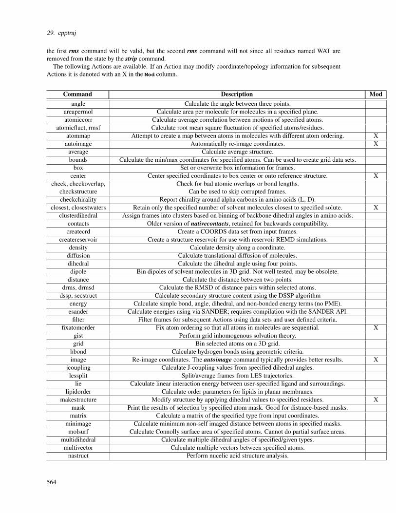
29. cpptraj
the first rms command will be valid, but the second rms command will not since all residues named WAT areremoved from the state by the strip command.
The following Actions are available. If an Action may modify coordinate/topology information for subsequentActions it is denoted with an X in the Mod column.
Command Description Modangle Calculate the angle between three points.
areapermol Calculate area per molecule for molecules in a specified plane.atomiccorr Calculate average correlation between motions of specified atoms.
atomicfluct, rmsf Calculate root mean square fluctuation of specified atoms/residues.atommap Attempt to create a map between atoms in molecules with different atom ordering. Xautoimage Automatically re-image coordinates. X
average Calculate average structure.bounds Calculate the min/max coordinates for specified atoms. Can be used to create grid data sets.
box Set or overwrite box information for frames.center Center specified coordinates to box center or onto reference structure. X
check, checkoverlap, Check for bad atomic overlaps or bond lengths.checkstructure Can be used to skip corrupted frames.checkchirality Report chirality around alpha carbons in amino acids (L, D).
closest, closestwaters Retain only the specified number of solvent molecules closest to specified solute. Xclusterdihedral Assign frames into clusters based on binning of backbone dihedral angles in amino acids.
contacts Older version of nativecontacts, retained for backwards compatibility.createcrd Create a COORDS data set from input frames.
createreservoir Create a structure reservoir for use with reservoir REMD simulations.density Calculate density along a coordinate.
diffusion Calculate translational diffusion of molecules.dihedral Calculate the dihedral angle using four points.dipole Bin dipoles of solvent molecules in 3D grid. Not well tested, may be obsolete.
distance Calculate the distance between two points.drms, drmsd Calculate the RMSD of distance pairs within selected atoms.
dssp, secstruct Calculate secondary structure content using the DSSP algorithmenergy Calculate simple bond, angle, dihedral, and non-bonded energy terms (no PME).esander Calculate energies using via SANDER; requires compilation with the SANDER API.
filter Filter frames for subsequent Actions using data sets and user defined criteria.fixatomorder Fix atom ordering so that all atoms in molecules are sequential. X
gist Perform grid inhomogenous solvation theory.grid Bin selected atoms on a 3D grid.
hbond Calculate hydrogen bonds using geometric criteria.image Re-image coordinates. The autoimage command typically provides better results. X
jcoupling Calculate J-coupling values from specified dihedral angles.lessplit Split/average frames from LES trajectories.
lie Calculate linear interaction energy between user-specified ligand and surroundings.lipidorder Calculate order parameters for lipids in planar membranes.
makestructure Modify structure by applying dihedral values to specified residues. Xmask Print the results of selection by specified atom mask. Good for distnace-based masks.matrix Calculate a matrix of the specified type from input coordinates.
minimage Calculate minimum non-self imaged distance between atoms in specified masks.molsurf Calculate Connolly surface area of specified atoms. Cannot do partial surface areas.
multidihedral Calculate multiple dihedral angles of specified/given types.multivector Calculate multiple vectors between specified atoms.
nastruct Perform nucelic acid structure analysis.
564

29.9. Action Commands
nativecontacts Calculate native contacts within a region or between two regions using a given reference.Can also be used to get min/max distances between groups of atoms.
outtraj Write frames to a trajectory file within a list of Actions.pairdist Calculate pair distribution function.pairwise Calculate pair-wise non-bonded energies.principal Calculate and optionally align system along principal axes. Xprojection Project coordinates along given eigenvectors.
pucker Calculate ring pucker using five or six points.radgyr, rog Calculate radius of gyration (and optionally tensor) for specified atoms.radial, rdf Calculate radial distribution function.
randomizeions Swap specified ions with randomly selected solvent molecules. Xreplicatecell Replicate unit cell in specified (or all) directions for specfied atoms and write to trajectory.rms, rmsd Perform best fit of coordinates to reference and calculate coordinate RMSD. X
Fitting can be disabled.rotate Rotate the system around X/Y/Z axes, a specified axis, or via given rotation matrices. X
runavg, Calculate the running average of coordinates over specified window size. Xrunningaverage
scale Scale coordinates in X/Y/Z directions by specified factors. Xsetvelocity Set velocities for specified atoms using Maxwellian distribution based on given temperature.
spam SPAM method for estimating relative free energies of waters in hydration shell around proteins. Xstfcdiffusion Alternative translational diffusion calculation which can calculate diffusion in specified regions.
strip Remove specified atoms from the system.surf Calculate the LCPO surface area of specified atoms. Can do partial surface areas.
symmrmsd Calculate symmetry-corrected RMSD. Xtemperature Calculate system temperature using velocities of specified atoms.
trans, translate Translate specified atoms by specified amounts in X/Y/Z directions. Xunstrip Undo all previous strip Action commands.unwrap Reverse of image; unwrap selected atoms so they have continuous trajectories. Xvector Calculate various types of vector quantities.
velocityautocorr Calculate velocity autocorrelation function.volmap Create volumetric map for specified coordinates; similar to grid but takes
into account atomic radii. Similar to VMD volmap.volume Calculate unit cell volume.
watershell Calculate the number of waters in the first and second solvation shells based on distance critera.
29.9.1. angle
angle [<dataset name>] <mask1> <mask2> <mask3> [out <filename>] [mass]
[<dataset name>] Output data set name.
<maskX> Three atom masks selecting atom(s) to calculate angle for.
[out <filename>] Output file name.
[mass] Use center of mass of atoms in <maskX> instead of geometric center.
Calculate angle (in degrees) between atoms in <mask1>, <mask2>, and <mask3>. For example, to calculate theangle between the first three atoms in the system:
angle A123 @1 @2 @3 out A123.agr
565
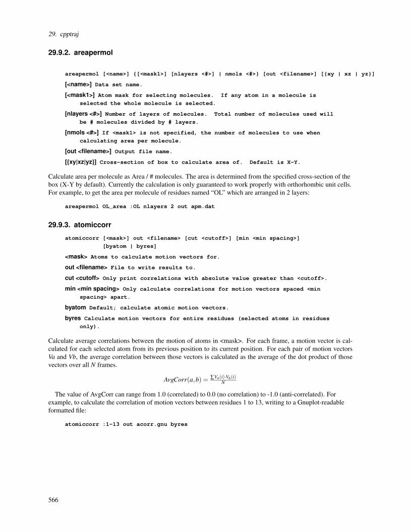
29. cpptraj
29.9.2. areapermol
areapermol [<name>] [<mask1>] [nlayers <#>] | nmols <#> [out <filename>] [xy | xz | yz]
[<name>] Data set name.
[<mask1>] Atom mask for selecting molecules. If any atom in a molecule is
selected the whole molecule is selected.
[nlayers <#>] Number of layers of molecules. Total number of molecules used will
be # molecules divided by # layers.
[nmols <#>] If <mask1> is not specified, the number of molecules to use when
calculating area per molecule.
[out <filename>] Output file name.
[xy|xz|yz] Cross-section of box to calculate area of. Default is X-Y.
Calculate area per molecule as Area / # molecules. The area is determined from the specified cross-section of thebox (X-Y by default). Currently the calculation is only guaranteed to work properly with orthorhombic unit cells.For example, to get the area per molecule of residues named “OL” which are arranged in 2 layers:
areapermol OL_area :OL nlayers 2 out apm.dat
29.9.3. atomiccorr
atomiccorr [<mask>] out <filename> [cut <cutoff>] [min <min spacing>]
[byatom | byres]
<mask> Atoms to calculate motion vectors for.
out <filename> File to write results to.
cut <cutoff> Only print correlations with absolute value greater than <cutoff>.
min <min spacing> Only calculate correlations for motion vectors spaced <min
spacing> apart.
byatom Default; calculate atomic motion vectors.
byres Calculate motion vectors for entire residues (selected atoms in residues
only).
Calculate average correlations between the motion of atoms in <mask>. For each frame, a motion vector is cal-culated for each selected atom from its previous position to its current position. For each pair of motion vectorsVa and Vb, the average correlation between those vectors is calculated as the average of the dot product of thosevectors over all N frames.
AvgCorr(a,b) = ∑Va(i)·Vb(i)N
The value of AvgCorr can range from 1.0 (correlated) to 0.0 (no correlation) to -1.0 (anti-correlated). Forexample, to calculate the correlation of motion vectors between residues 1 to 13, writing to a Gnuplot-readableformatted file:
atomiccorr :1-13 out acorr.gnu byres
566
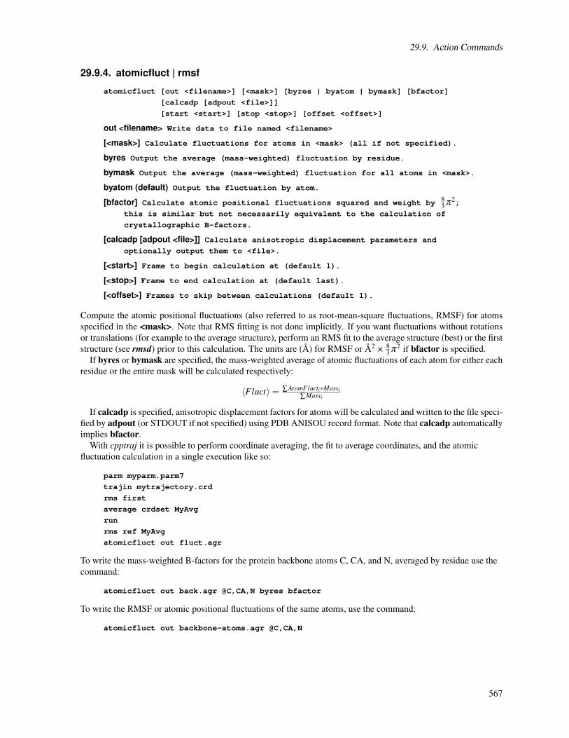
29.9. Action Commands
29.9.4. atomicfluct | rmsf
atomicfluct [out <filename>] [<mask>] [byres | byatom | bymask] [bfactor]
[calcadp [adpout <file>]]
[start <start>] [stop <stop>] [offset <offset>]
out <filename> Write data to file named <filename>
[<mask>] Calculate fluctuations for atoms in <mask> (all if not specified).
byres Output the average (mass-weighted) fluctuation by residue.
bymask Output the average (mass-weighted) fluctuation for all atoms in <mask>.
byatom (default) Output the fluctuation by atom.
[bfactor] Calculate atomic positional fluctuations squared and weight by 83 π2;
this is similar but not necessarily equivalent to the calculation of
crystallographic B-factors.
[calcadp [adpout <file>]] Calculate anisotropic displacement parameters and
optionally output them to <file>.
[<start>] Frame to begin calculation at (default 1).
[<stop>] Frame to end calculation at (default last).
[<offset>] Frames to skip between calculations (default 1).
Compute the atomic positional fluctuations (also referred to as root-mean-square fluctuations, RMSF) for atomsspecified in the <mask>. Note that RMS fitting is not done implicitly. If you want fluctuations without rotationsor translations (for example to the average structure), perform an RMS fit to the average structure (best) or the firststructure (see rmsd) prior to this calculation. The units are (Å) for RMSF or Å2 × 8
3 π2 if bfactor is specified.If byres or bymask are specified, the mass-weighted average of atomic fluctuations of each atom for either each
residue or the entire mask will be calculated respectively:
〈Fluct〉= ∑AtomFlucti∗Massi∑Massi
If calcadp is specified, anisotropic displacement factors for atoms will be calculated and written to the file speci-fied by adpout (or STDOUT if not specified) using PDB ANISOU record format. Note that calcadp automaticallyimplies bfactor.
With cpptraj it is possible to perform coordinate averaging, the fit to average coordinates, and the atomicfluctuation calculation in a single execution like so:
parm myparm.parm7
trajin mytrajectory.crd
rms first
average crdset MyAvg
run
rms ref MyAvg
atomicfluct out fluct.agr
To write the mass-weighted B-factors for the protein backbone atoms C, CA, and N, averaged by residue use thecommand:
atomicfluct out back.agr @C,CA,N byres bfactor
To write the RMSF or atomic positional fluctuations of the same atoms, use the command:
atomicfluct out backbone-atoms.agr @C,CA,N
567

29. cpptraj
29.9.5. atommap
atommap <target> <reference> [mapout <filename>] [maponly]
[rmsfit [ rmsout <rmsout> ]]
<target> Reference structure whose atoms will be remapped.
<reference> Reference structure that <target> should be mapped to.
mapout <filename> Write atom map to <filename> with format:
TargetAtomNumber TargetAtomName ReferenceAtomNumber ReferenceAtomName
Target atoms that cannot be mapped to a reference atom are denoted “---”.
maponly Write atom map but do not reorder atoms.
rmsfit Any input frames using the same topology as <target> will be RMS fit to
<reference> using whatever atoms could be mapped.
rmsout <rmsout> If rmsfit specified, write resulting RMSDs to <rmsout>.
Attempt to map the atoms of <target> to those of <reference> based on structural similarity. This is useful e.g.when there are two files containing the same structure but with different atom names or atom ordering. Both<target> and <reference> need to have been read in with a previous reference command. The state will then bemodified so that any trajectory read in with the same parameter file as <target> will have its atoms mapped (i.e.reordered) to match those of <reference>. If the number of atoms that can be mapped in <target> are less thanthose in <reference>, the reference structure specified by <reference> will be modified to include only mappedatoms; this is useful if for example the reference structure is protonated with respect to the target. The rmsfitkeyword is useful in cases where the atom mapping will not be complete (e.g. two ligands with the same scaffoldbut different substituents).
For example, say you have the same ligand structure in two files, Ref.mol2 and Lig.mol2, but the atom orderingin each file is different. To map the atoms in Lig.mol2 onto those of Ref.mol2 so that Lig.mol2 has the sameordering as Ref.mol2:
parm Lig.mol2
reference Lig.mol2
parm Ref.mol2
reference Ref.mol2 parmindex 1
atommap Lig.mol2 Ref.mol2 mapout atommap.dat
trajin Lig.mol2
trajout Lig.reordered.mol2 mol2
29.9.6. autoimage
autoimage [<mask> | anchor <mask> [fixed <mask>] [mobile <mask>]]
[origin] [firstatom] [familiar | triclinic]
[<mask> | anchor <mask>] Molecule to image around; this is the molecule that will
be centered. Default is first molecule.
[fixed <mask>] Molecules that should remain ’fixed’ to the anchor molecule;
default is all non-ion/non-solvent molecules.
[mobile <mask>] Molecules that can be freely imaged; default is all ion/solvent
molecules.
[origin] Center anchor at the origin; if not specified, center at box center.
[firstatom] Image based on molecule first atom; default is to image by molecule
center of mass.
[familiar] Image to familiar truncated-octahedral shape; this is on by default if
the original cell is truncated octahedron.
568

29.9. Action Commands
[triclinic] Force general triclinic imaging.
Automatically center and image (by molecule) a trajectory with periodic boundaries. For most cases just spec-ifying ’autoimage’ alone is sufficient. The ’anchor’ molecule (default the first molecule) will be centered; all’fixed’ molecules will be imaged only if imaging brings them closer to the ’anchor’ molecule; default for ’fixed’molecules is all non-solvent non-ion molecules. All other molecules (referred to as ’mobile’) will be imaged freely.
In general, the ’anchor’ molecule should be one that has the smallest distance to all ’fixed’ molecules.
29.9.7. average
average crdset <set name> | <filename> [<mask>]
[start <start>] [stop <stop>] [offset <offset>]
[Trajout Args]
<filename> If specified, write averaged coordinates to <filename> (not
compatible with crdset).
crdset <set name> If specified, save averaged coordinates to COORDS set <set
name> (not compatible with <filename>).
[<mask>] Average coordinates in <mask> (all atoms if not specified).
[<start>] Frame to begin calculation at (default 1).
[<stop>] Frame to end calculation at (default last).
[<offset>] Frames to skip between calculations (default 1).
[Trajout args] Output trajectory format argument(s) (default Amber Trajectory).
Calculate the average of input coordinates and write out to file named <filename> or save to COORDS set named<set name> in any trajectory format cpptraj recognizes (Amber Trajectory if not specified). If the number ofatoms in <mask> are less than the total number of atoms, the topology will be stripped to match <mask>.
Note that since coordinates are being averaged over many frames, resulting structures may appear distorted. Forexample, if one averages the coordinates of a freely rotating methyl group the average position of the hydrogenatoms will be close to the center of rotation. Also note that typically one will want to remove global rotational andtranslation movement prior to this command by using e.g. the rms ( 29.9.60 on page 607) command.
Any arguments that are valid for the trajout command ( 29.8.5 on page 561) can be passed to this command inorder to control the format of the output coordinates. For example, to write out a PDB file containing the averagedcoordinates over all frames:
average test.pdb pdb
To write out a mol2 file containing only the averaged coordinates of residues 1 to 10 for frames 1 to 100:
average test.mol2 mol2 start 1 stop 100 :1-10
To create an average structure of atoms named CA and then use it as a reference for an rms command in asubsequent run:
trajin Input.nc
average crdset MyAvg @CA
run
rms ref MyAvg @CA out RmsToAvg.dat
run
29.9.8. avgcoord
This command is deprecated. Use ’vector center’ (optionally with keyword ’magnitude’) instead.
569

29. cpptraj
29.9.9. bounds
bounds [<mask>] [out <filename>]
[dx <dx> [dy <dy>] [dz <dz>] name <gridname> [offset <bin offset>]]
[<mask>] Mask of atoms to determine bounds of.
[out <filename>] File to write bounds to (default STDOUT if not specified).
[dx <dx> [dy <dy>] [dz <dz>]] Triggers creation of a grid data set from bounds.
Spacings of generated grid in the X, Y and Z directions. If only dx is
specified <dx> will be used for <dy> and <dz> as well.
[name <gridname>] Name of generated grid data set.
[offset <bin offset>] Number of bins to add/subtract in each direction to generated
grid.
Calculate the boundaries (i.e. the max/min X/Y/Z coordinates) of atoms in <mask> and write to <filename>(STDOUT if not specified). Useful for determining dimensions for the grid command, and can be used to generatea grid data set that can be used by grid (see 29.9.33 on page 585).
29.9.10. box
box [x <xval>] [y <yval>] [z <zval>] [alpha <a>] [beta <b>] [gamma <g>]
[nobox] [truncoct]
[x <xval>] [y <yval>] [z <zval>] Change box length(s) to specified value(s).
[alpha <a>] [beta <b>] [gamma <g>] Change box angle(s) to specified value(s).
[nobox] Remove any existing box information.
[truncoct] Set box angles to truncated octahedron.
Modify box information during trajectory processing. Note that this will permanently modify the box informationfor topology files during trajectory processing as well. It is possible to modify any number of the box parameters(e.g. only the Z length can be modified if desired while leaving all other parameters intact).
29.9.11. center
center [<mask>] [origin] [mass]
[ reference | ref <name> | refindex <#> [<refmask>]]
[<mask>] Center based on atoms in mask; default is all atoms.
[origin] Center to origin (0, 0, 0); default is center to box center (X/2, Y/2,
Z/2).
[mass] Use center of mass instead of geometric center.
[reference | ref <name> | refindex <#> [<refmask]] Center using coordinates in specified
reference structure selected by <refmask> (<mask> if not specified.
Move all atoms so that the center of the atoms in <mask> is centered at the specified location: box center (default),coordinate origin, or reference coordinates.
For example, to move all coordinates so that the center of mass of residue 1 is at the center of the box:
center :1 mass
570

29.9. Action Commands
29.9.12. check | checkoverlap | checkstructure
check [<mask>] [around <mask2>] [reportfile <report>] [noimage] [skipbadframes]
[offset <offset>] [cut <cut>] [nobondcheck] [silent]
[<mask>] Check structure of atoms in <mask> (all if not specified).
[around <mask2>] If specified, only check for problems between atoms in <mask>
and atoms in <mask2>.
[reportfile <report>] Write any problems found to <report> (STDOUT if not
specified).
[noimage] Do not image distances.
[skipbadframes] If errors are encountered for a frame, subsequent
actions/trajectory output will be skipped.
[offset <offset>] Report bond lengths greater than the equilibrium value plus
<offset> (default 1.0 Å)
[cut <cut>] Report atoms closer than <cut> (default 0.8 Å).
[nobondcheck] Check overlaps only.
[silent] Do not print information for bad frames - useful in conjunction with the
skipbadframes option.
Check the structure and report problems related to atomic overlap/unusual bond length. Problems are reportedwhen any two atoms in the mask are closer than <cut>. If bonds are being checked then bond lengths greater thantheir equilibrium value + <offset> are reported as well. This command can also be used to skip corrupted framesin a trajectory during processing. For example, if this message is encountered:
Warning: Frame 10 coords 1 & 2 overlap at origin; may be corrupt.
One could use check so that e.g. a subsequent distance command is not processed for bad frames:
check @1,2 skipbadframes silent
distance d1 :1 :10
Usually frame corruption can be detected using only a few atoms, but this may not catch all types of corruption.The more atoms that are used the better the corruption detection will be, but the slower it will be to process thecommand. Typically a good procedure to follow when corruption is suspected is to run check using all importantatoms (e.g. all solute heavy atoms) with the skipbadframes keyword followed by a trajout command to write allnon-corrupt frames, for example:
trajin corrupted.crd
check :1-13 skipbadframes silent
trajout fixed.corrupted.nc
29.9.13. checkchirality
checkchirality [<name>] [<mask>] [out <filename>]
[<name>] Data set name.
[<mask>] Atoms to check.
[out <filename>] File to write results to.
DataSet Aspects:
[L] Number of frames ’L’ for each residue.
[D] Number of frames ’D’ for each resdiue.
571
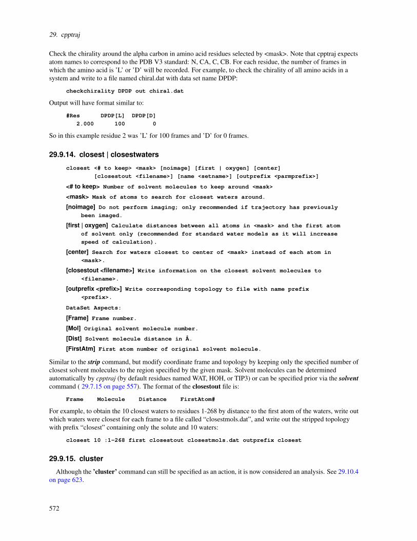
29. cpptraj
Check the chirality around the alpha carbon in amino acid residues selected by <mask>. Note that cpptraj expectsatom names to correspond to the PDB V3 standard: N, CA, C, CB. For each residue, the number of frames inwhich the amino acid is ’L’ or ’D’ will be recorded. For example, to check the chirality of all amino acids in asystem and write to a file named chiral.dat with data set name DPDP:
checkchirality DPDP out chiral.dat
Output will have format similar to:
#Res DPDP[L] DPDP[D]
2.000 100 0
So in this example residue 2 was ’L’ for 100 frames and ’D’ for 0 frames.
29.9.14. closest | closestwaters
closest <# to keep> <mask> [noimage] [first | oxygen] [center]
[closestout <filename>] [name <setname>] [outprefix <parmprefix>]
<# to keep> Number of solvent molecules to keep around <mask>
<mask> Mask of atoms to search for closest waters around.
[noimage] Do not perform imaging; only recommended if trajectory has previously
been imaged.
[first | oxygen] Calculate distances between all atoms in <mask> and the first atom
of solvent only (recommended for standard water models as it will increase
speed of calculation).
[center] Search for waters closest to center of <mask> instead of each atom in
<mask>.
[closestout <filename>] Write information on the closest solvent molecules to
<filename>.
[outprefix <prefix>] Write corresponding topology to file with name prefix
<prefix>.
DataSet Aspects:
[Frame] Frame number.
[Mol] Original solvent molecule number.
[Dist] Solvent molecule distance in Å.
[FirstAtm] First atom number of original solvent molecule.
Similar to the strip command, but modify coordinate frame and topology by keeping only the specified number ofclosest solvent molecules to the region specified by the given mask. Solvent molecules can be determinedautomatically by cpptraj (by default residues named WAT, HOH, or TIP3) or can be specified prior via the solventcommand ( 29.7.15 on page 557). The format of the closestout file is:
Frame Molecule Distance FirstAtom#
For example, to obtain the 10 closest waters to residues 1-268 by distance to the first atom of the waters, write outwhich waters were closest for each frame to a file called “closestmols.dat”, and write out the stripped topologywith prefix “closest” containing only the solute and 10 waters:
closest 10 :1-268 first closestout closestmols.dat outprefix closest
29.9.15. cluster
Although the ’cluster’ command can still be specified as an action, it is now considered an analysis. See 29.10.4on page 623.
572

29.9. Action Commands
29.9.16. clusterdihedral
clusterdihedral [phibins <N>] [psibins <M>] [out <outfile>]
[dihedralfile <dfile> | <mask>]
[framefile <framefile>] [clusterinfo <infofile>]
[clustervtime <cvtfile>] [cut <CUT>]
Cluster frames in a trajectory using dihedral angles. To define which dihedral angles will be used for clusteringeither an atom mask or an input file specified by the dihedralfile keyword should be used. If dihedral file is used,each line in the file should contain a dihedral to be binned with format:
ATOM#1 ATOM#2 ATOM#3 ATOM#4 #BINS
where the ATOM arguments are the atom numbers (starting from 1) defining the dihedral and #BINS is the numberof bins to be used (so if #BINS=10 the width of each bin will be 36º). If an atom mask is specified, only proteinbackbone dihedrals (Phi and Psi defined using atom names C-N-CA-C and N-CA-C-N) within the mask will beused, with the bin sizes specified by the phibins and psibins keywords (default for each is 10 bins).
Output will either be written to STDOUT or the file specified by the out keyword. First, information aboutwhich dihedrals were clustered will be printed. Then the number of clusters will be printed, followed by detailedinformation of each cluster. The clusters are sorted from most populated to least populated. Each cluster line hasformat
Cluster CLUSTERNUM CLUSTERPOP [ dihedral1bin, dihedral2bin ... dihedralNbin ]
followed by a list of frame numbers that belong to that cluster. If a cutoff is specified by cut, only clusters withpopulation greater than CUT will be printed.
If specified by the clustervtime keyword, the number of clusters for each frame will be printed to <cvtfile>. Ifspecified by the framefile keyword, a file containing cluster information for each frame will be written withformat
Frame CLUSTERNUM CLUSTERSIZE DIHEDRALBINID
where DIHEDRALBINID is a number that identifies the unique combination of dihedral bins this cluster belongsto (specifically it is a 3*number-of-dihedral-characters long number composed of the individual dihedral bins).
If specified by the clusterinfo keyword, a file containing information on each dihedral and each cluster will beprinted. This file can be read by SANDER for use with REMD with a structure reservoir (-rremd=3). The file,which is essentially a simplified version of the main output file, has the following format:
#DIHEDRALS
dihedral1_atom1 dihedral1_atom2 dihedral1_atom3 dihedral1_atom4
...
#CLUSTERS
CLUSTERNUM1 CLUSTERSIZE1 DIHEDRALBINID1
...
29.9.17. contacts
contacts [ first | reference | ref <ref> | refindex <#> ] [byresidue]
[out <filename>] [time <interval>] [distance <cutoff>] [<mask>]
NOTE: Users are encouraged to try the nativecontacts command ( on page 600), an update version of this com-mand.
For each atom given in mask, calculate the number of other atoms (contacts) within the distance cutoff. Thedefault cutoff is 7.0 A. Only atoms in mask are potential interaction partners (e.g., a mask @CA will evaluate onlycontacts between CA atoms). The results are dumped to filename if the keyword “out” is specified. Thereby,the time between snapshots is taken to be interval. In addition to the number of overall contacts, the number of
573

29. cpptraj
native contacts is also determined. Native contacts are those that have been found either in the first snapshot ofthe trajectory (if the keyword “first” is specified) or in a reference structure (if the keyword “reference” isspecified). Finally, if the keyword “byresidue” is provided, results are output on a per-residue basis for eachsnapshot, whereby the number of native contacts is written to filename.native.
29.9.18. createcrd
See 29.5.4 on page 544.
29.9.19. createreservoir
createreservoir <filename> ene <energy data set> [bin <cluster bin data set>]
temp0 <temp0> iseed <iseed> [velocity]
[parm <parmfile> | parmindex <#>] [title <title>]
<filename> File name of the reservoir to create.
ene <energy data set> Data set with energies corresponding to frames.
[bin <cluster bin data set>] Data set with bin numbers (for RREMD=3).
temp0 <temp0> Reservoir temperature.
iseed <iseed> Reservoir random number seed.
[velocity] Include velocities in the reservoir.
[parm <parmfile> | parmindex <#>] Associated topology.
[title <title>] Reservoir title.
Create structure reservoir for use with reservoir REMD simulations using energies in <energy data set>, temper-ature <temp0> and random seed <iseed> Include velocities if [velocity] is specified. If <cluster bin data set> isspecified from e.g. a previous ’clusterdihedral’ command, the reservoir can be used for non-Boltzmann reservoirREMD (rremd==3).
29.9.20. density
density out <filename> [delta <resolution>] [x|y|z]
[number|mass|charge|electron] [efile <filename>]
<mask1> ... <maskN>
out Output file for histogram: relative distances vs. densities for each
mask.
delta Resolution, i.e. determines number of slices. (0.25 Å)
x|y|z Coordinate for density calculation. (z)
number|mass|charge|electron Number, mass, partial charge (q) or electron (Ne - q)
density. To convert the electron density to e-/Å3 divide by the (average)
area spanned by the other two dimensions. (number)
efile Optional file with electron numbers Ne for each atom type.
mask1 ... maskN Arbitrary number of masks for atom selection, the output will
contain a column for each mask.
Calculate specified density for system. Defaults are shown in parentheses above. If efile is not supplied thecommand assumes that atom types starting with ’H’, ’C’, ’N’, ’O’, ’P’ and ’S’ are the actual elements. The formatof the file is as follows. Comments are lines starting with ’#’ or empty lines. All other lines must contain the atomtype followed by an integer number for the electron number. Entries must be separated by spaces or ’=’. Exampleinput:
574

29.9. Action Commands
density out number_density.dat number delta 0.25 ":POPC@P1" ":POPC@N" \
":POPC@C2" ":POPC"
density out mass_density.dat mass delta 0.25 ":POPC@P1" ":POPC@N" \
":POPC@C2" ":POPC"
density out charge_density.dat charge delta 0.25 ":POPC@P1" ":POPC@N" \
":POPC@C2" ":POPC"
density out electron_density.dat electron delta 0.25 efile Nelec.in \
":POPC@P1" ":POPC@N" ":POPC@C2" ":POPC" ":TIP3" \
":POPC | :TIP3" "*"
density out ion_density.dat number delta 0.25 ":SOD" ":CLA"
See also $AMBERHOME/AmberTools/test/cpptraj/Test_Density.
29.9.21. diffusion
Note that although the syntax for diffusion has changed as of version 16, the old syntax is still supported.
diffusion [out <filename> | separateout <suffix>] [time <time per frame>] [noimage]
[<mask>] [<set name>] [individual] [diffout <filename>] [nocalc]
[out <filename>] Write mean-square displacement (MSD) data set output to file
specified by <filename>.
[separateout <suffix>] Write each MSD data set type to files with suffix <suffix>;
see description below.
[time <time_per_frame>] Time in-between each coordinate frame in ps; default is
1.0.
[noimage] If specified do not perform imaging. If this is specified coordinates
should be unwrapped prior to this command.
[<mask>] Mask of atoms to calculate diffusion for; default all atoms.
[<set name>] MSD data set name.
[individual] Write diffusion for each individual atom as well as average diffusion
for atoms in mask.
[diffout <filename>] Write diffusion contants calculated from fits of MSD data sets
to <filename>.
[nocalc] Do not calculate diffusion constants.
DataSet Aspects:
[X] MSD(s) in the X direction.
[Y] MSD(s) in the Y direction.
[Z] MSD(s) in the Z direction.
[R] Overall MSD(s).
[A] Overall displacement(s).
[D] Diffusion constants.
[Label] Diffusion constant lablels.
[Slope] Linear regression slopes.
[Intercept] Linear refression Y-intercepts.
[Corr] Linear regression correlation coefficients.
575

29. cpptraj
Compute mean square displacement (MSD) plots (using distance traveled from initial position) for the atoms in<mask>. By default only the diffusion averaged over all atoms in <mask> is calculated; if individual is specifieddiffusion for individual atoms is calculated as well.
In order to correctly calculate diffusion molecules should take continuous paths, so imaging of atoms is autoimat-ically performed. If the trajectory is already unwrapped (or the unwrap command is used prior to this command)the noimage keyword can be used.
The following types of displacements are calculated. If separateout is specfied the following files will becreated:
x_<suffix> Mean square displacement(s) in the X direction (in Å2/ps).
y_<suffix> Mean square displacement(s) in the Y direction (in Å2/ps).
z_<suffix> Mean square displacement(s) in the Z direction (in Å2/ps).
r_<suffix> Overall mean square displacement(s) (in Å2/ps).
a_<suffix> Total distance traveled (in Å/ps).
The diffusion coefficient D can be calculated using the Einstein relation:
2nD = limt→∞
MSDt
Where n is the number of dimensions; for overall MSD n = 3, for single dimension MSD (e.g. X) n = 1, etc.Unless nocalc is specified, the diffusion constant is calculated automatically from MSD data sets (and written tothe file specified by diffout) in the following manner. The slope the plot of MSD versus time is obtained via linearregression. To convert from units of Å2/ps to 1x10⁻⁵ cm2/s, the slope is multiplied by 10.0/(2n). Both the calculateddiffusion constants as well as the results of the fit are reported.
Due to the fact that diffusion is currently calculated from initial positions only, diffusion calculated for smallnumbers of atoms will be inherently stochastic, so the results are most sensible when averaged over many atoms;for example, the diffusion of water should be calculated using all waters in the system.
For example, to calculate the diffusion of water in a system:
diffusion :WAT@O out WAT_O.agr WAT_O diffout DC.dat
29.9.22. dihedral
dihedral [<name>] <mask1> <mask2> <mask3> <mask4> [out <filename>] [mass]
[type alpha|beta|gamma|delta|epsilon|zeta|chi|c2p|h1p|phi|psi|omega|pchi]
[range360]
[<name>] Output data set name.
<maskX> Four atom masks selecting atom(s) to calculate dihedral for.
[out <filename>] Output file name.
[mass] Use center of mass of atoms in <maskX>; default is geometric center.
[range360] Output dihedral angle values from 0 to 360 degrees instead of -180 to
180 degrees.
[type <type>] Label dihedral as <type> for use with statistics analysis; note
’chi’ is nucleic acid chi and ’pchi’ is protein chi.
Calculate dihedral angle (in degrees) between the planes defined by atoms in <mask1>, <mask2>, <mask3> and<mask2>, <mask3>, <mask4>.
576

29.9. Action Commands
29.9.23. dihedralscan
This command has been replaced by permutedihedrals; see 29.6.14 on page 548. To calculate multiple dihedralangles see the multidihedral command.
29.9.24. dipole
dipole <filename> data <dsname> | <nx> <dx> <ny> <dy> <nz> <dz> [gridcenter <cx> <cy> <cz>]
[box|origin|center <mask>] [negative] [name <gridname>]
<mask1> origin | box [max <max_percent>]
NOTE: This command is not well-tested and may be obsolete.Same as grid (see 29.9.33 on page 585 below) except that dipoles of the solvent molecules are binned. The
output file format is for Chris Bayly’s discern delegate program that comes with Midas/Plus. Consult the code inAction_Dipole.cpp for more information.
29.9.25. distance
distance [<name>] <mask1> <mask2> [out <filename>] [geom] [noimage] [type noe]
Options for ’type noe’:
[bound <lower> bound <upper>] [rexp <expected>] [noe_strong] [noe_medium] [noe_weak]
[<name>] Output data set name
<maskX> Two atom masks selecting atom(s) to calculate distance between.
[out <filename>] Output filename.
[geom] Use geometric center of atoms in <mask1>/<mask2>; default is to use
center of mass.
[noimage] Do not image distances across periodic boundaries.
[type noe] Mark distance as ’noe’ for use with statistics analysis.
[bound <lower> bound <upper>] Lower and upper bounds for NOE (in Angstroms);
must specify both.
[rexp <expected>] Expected value for NOE (in Angstroms); if not given
’(<lower> + <upper>)’ / 2.0 is used.
[noe_strong] Set lower and upper bounds to 1.8 and 2.9 Å respectively.
[noe_medium] Set lower and upper bounds to 2.9 and 3.5 Å respectively.
[noe_weak] Set lower and upper bounds to 3.5 and 5.0 Å respectively.
Calculate distance between the center of mass of atoms in <mask1> to atoms in <mask2>. If geom is specified usethe geometric center instead. For periodic systems imaging is turned on by default; the noimage keyword disablesimaging.
A distance can be labeled using ’type noe’ for further analysis as an NOE using the ’statistics’ analysis com-mand.
29.9.26. drms | drmsd (distance RMSD)
drmsd [<dataset name>] [<mask> [<refmask>]] [out <filename>]
[ first | ref <refname> | refindex <#> |
reftraj <trajname> [parm <trajparm> | parmindex <parm#>] ]
[<dataset name>] Output data set name.
[<mask>] Atoms to calculate DRMSD for.
577

29. cpptraj
[<refmask>] Mask corresponding to atoms in reference; if not specified, <mask>
is used.
[out <filename>] Output file name.
[first] Use the first trajectory frame processed as reference.
[reference] Use the first previously read in reference structure.
[ref <refname>] Use previously read in reference structure specified by
<refname>.
[refindex <#>] Use previously read in reference structure specified by <#> (based
on order read in).
previous Use frame prior to current frame as reference.
reftraj <name> Use frames from COORDS set <name> or read in from trajectory file
<name> as references. Each frame from <name> is used in turn, so that
frame 1 is compared to frame 1 from <name>, frame 2 is compared to frame 2
from <name> and so on. If <trajname> runs out of frames before processing
is complete, the last frame of <trajname> continues to be used as the
reference.
parm <parmname> | parmindex <#> If reftraj specifies a file associate
trajectory <name> with specified topology; if not specified the first
topology is used.
Calculate the distance RMSD (i.e. the RMSD of all pairs of internal distances) between atoms in the frame definedby <mask> (all if no <mask> specified) to atoms in a reference defined by <refmask> (<mask> if <refmask> notspecified). Both <mask> and <refmask> must specify the same number of atoms, otherwise an error will occur.
Because this method compares pairs of internal distances and not absolute coordinates, it is not sensitive totranslations and rotations the way that a no-fit RMSD calculation is. It can be more time consuming however, as(N2-N)/2 distances must be calculated and compared for both the target and reference structures.
For example, to get the DRMSD of a residue named LIG to its structure in the first frame read in:
drmsd :LIG first out drmsd.dat
29.9.27. dssp
See 29.9.68 on page 611.
29.9.28. energy
energy [<name>] [<mask1>] [out <filename>]
[bond] [angle] [dihedral] [nb14] [nonbond]
[<name>] Data set name.
[<mask1>] Mask of atoms to calculate energy for.
[out <filename>] File to write results to.
[bond] Calculate bond energy.
[angle] Calculate angle energy.
[dihedral] Calculate dihedral energy.
[nb14] Calculate nonbonded 1-4 energy.
[nonbond] Calculate nonbonded energy.
DataSet Aspects:
[bond] Bond energy.
578
29.9. Action Commands
[angle] Angle energy.
[dih] Dihedral energy.
[vdw14] 1-4 van der Waals energy.
[elec14] 1-4 electrostatic energy.
[vdw] van der Waals energy.
[elec] Electrostatic energy.
[total] Total energy.
Calculate the energy for atoms in <mask>. If no terms are specified, all terms are calculated. Note that the non-bonded energy terms do not take into account periodicity and there is no distance cut-off. This also requires thatthe associated topology file have parameters for any of the calculated terms.
For example, to calculate all energy terms and write to a Grace-format file:
parm DPDP.parm7
trajin DPDP.nc
energy DPDP out ene.agr
29.9.29. esander
esander [<name>] [out <filename>] [saveforces] [parmname <file>] [<namelist vars> ...]
[<name>] Data set name.
[out <filename>] File to write results to.
[saveforces] If specified, save forces to frames. Requires writing frames in
NetCDF format.
[parmname <file>] Name of temporary topology file (default:
’CpptrajEsander.parm7’).
[<namelist vars>] Namelist variables supported by the sander API in format ’var
<value>’; see below.
Calculate energies for input frames using the sander API. This can be considered as a faster alternative to energypost-processing with sander (imin = 5). Currently the following sander namelist variables are supported: extidel,intdiel, rgbmax, saltcon, cut, dielc, igb, alpb, gbsa, lj1264, ipb, inp, vdwmeth, ew_type, ntb, ntf, ntc.
If ntb/cut/igb are not specified cpptraj will attempt to pick reasonable values based on the input system. Thedefaults for a non-periodic system are ntb=0, cut=9999.0, igb=1. The defaults for a periodic system are ntb=1,cut=8.0, igb=0.
For example, to calculate energies for a non-periodic system using igb=1 (the default) with GB surface areaturned on (gbsa=1):
parm DPDP.parm7
trajin DPDP.nc
esander DPDP out Edpdp.dat gbsa 1
29.9.30. filter
filter <dataset1 arg> min <min1> max <max1>
[<dataset2 arg> min <min2> max <max2> ...]
[out <file> [name <setname>]]
<datasetX arg> Data set name(s) to use for filtering
min <minX> Allow values greater than <min> in dataset X.
579
29. cpptraj
max <maxX> Allow values greater than <max> in dataset X.
[out <file>] File containing 1 for frames that were allowed, 0 for frames that
were filtered.
[name <setname>] Filtered data set name containing 1 for allowed frames, 0 for
filtered frames.
For all following actions, only include frames that are between <min> and <max> of data sets in <dataset arg>.There must be at least one <min> and <max> argument, and there must be as many <min>/<max> arguments asthere are specified data sets. For example, to write only frames in-between an RMSD of 0.7-0.8 Angstroms for agiven input trajectory:
trajin ../tz2.truncoct.nc
rms R1 first :2-11
filter R1 min 0.7 max 0.8 out filter.dat
outtraj maxmin.crd
The output trajectory will only contain frames that meet the RMSD requirement, and the filter.dat file can be usedto see which frames those were that were output.
A similar command that can be used with data that already exists (e.g. it has been read in with readdata) isdatafilter (see page 546).
29.9.31. fixatomorder
fixatomorder [outprefix <name>]
Cpptraj (and most of Amber) expects that atom indices in molecules to increase monotonically. However, oc-casionally atom indices in molecules can become disordered. This command fixes atom ordering so that allatoms in molecules are sequential. The outprefix keyword will write out the re-ordered topology with name<name>.<original name>.
29.9.32. gist (Grid Inhomogeneous Solvation Theory)
gist [doorder] [doeij] [refdens <rdval>]
[gridcntr <xval> <yval> <zval>] [griddim <xval> <yval> <zval>]
[gridspacn <spaceval>] [out <filename>]
Grid Inhomogeneous Solvation Theory [526, 527] (GIST) is a method for analyzing the structure and thermody-namics of solvent in the vicinity of a solute molecule. The current implementation works for only water, but themethod can be generalized to other solvents whose molecules are rigid like water, such as chloroform or dimethyl-sulfoxide (DMSO). GIST post-processes explicit solvent simulation data to create a three-dimensional mapping ofwater density and thermodynamic properties within a region of interest, which is defined by a user-specified 3Drectangular grid. The small grid boxes are referred to as voxels, and each voxel is associated with solvent proper-ties. (See Fig. 29.1.) The GIST implementation incorporated into AmberTools cpptraj also calculates a number ofother local water properties, as listed below. GIST works for the nonpolarizable water models currently supportedby AMBER. In order to carry out a GIST calculation, you must have a trajectory file generated with explicit water,as well as the corresponding prmtop file. To generate the most readily interpretable results, it is recommended thatthe solute (e.g., a protein) be restrained into essentially one conformation. GIST will then provide informationabout the structure and thermodynamics of the solvent for that conformation. For a room-temperature simulationof a solvent-exposed binding site, and a grid-spacing of 0.5 Å, it is recommended that the simulation be at least10-20 ns in duration, and it is also a good idea to check for convergence of the GIST properties you are interestedin by loading and then processing successively more frames of your trajectory file. Because GIST assumes that thesolute of interest comprises all molecules in the simulation that are not waters, it is a good idea to remove all coun-terions and cosolutes with cpptraj’s strip command before running GIST. A sample series of cpptraj commands forrunning GIST is provided below.
580
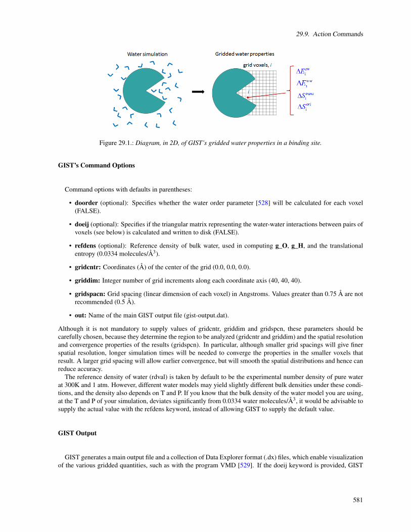
29.9. Action Commands
Figure 29.1.: Diagram, in 2D, of GIST’s gridded water properties in a binding site.
GIST’s Command Options
Command options with defaults in parentheses:
• doorder (optional): Specifies whether the water order parameter [528] will be calculated for each voxel(FALSE).
• doeij (optional): Specifies if the triangular matrix representing the water-water interactions between pairs ofvoxels (see below) is calculated and written to disk (FALSE).
• refdens (optional): Reference density of bulk water, used in computing g_O, g_H, and the translationalentropy (0.0334 molecules/Å3).
• gridcntr: Coordinates (Å) of the center of the grid (0.0, 0.0, 0.0).
• griddim: Integer number of grid increments along each coordinate axis (40, 40, 40).
• gridspacn: Grid spacing (linear dimension of each voxel) in Angstroms. Values greater than 0.75 Å are notrecommended (0.5 Å).
• out: Name of the main GIST output file (gist-output.dat).
Although it is not mandatory to supply values of gridcntr, griddim and gridspcn, these parameters should becarefully chosen, because they determine the region to be analyzed (gridcntr and griddim) and the spatial resolutionand convergence properties of the results (gridspcn). In particular, although smaller grid spacings will give finerspatial resolution, longer simulation times will be needed to converge the properties in the smaller voxels thatresult. A larger grid spacing will allow earlier convergence, but will smooth the spatial distributions and hence canreduce accuracy.
The reference density of water (rdval) is taken by default to be the experimental number density of pure waterat 300K and 1 atm. However, different water models may yield slightly different bulk densities under these condi-tions, and the density also depends on T and P. If you know that the bulk density of the water model you are using,at the T and P of your simulation, deviates significantly from 0.0334 water molecules/Å3, it would be advisable tosupply the actual value with the refdens keyword, instead of allowing GIST to supply the default value.
GIST Output
GIST generates a main output file and a collection of Data Explorer format (.dx) files, which enable visualizationof the various gridded quantities, such as with the program VMD [529]. If the doeij keyword is provided, GIST
581

29. cpptraj
also writes out a matrix of water-water interactions between pairs of voxels. In addition, run details are written tostdout, which can be redirected into a log file.
Note that a number of quantities are written out as both densities and normalized quantities. For example,the output file includes both the solute-water energy density and the normalized (per water) solute-water energy.In all cases, the normalized quantity at voxel i, Xi,norm is related to the corresponding density, Xi,dens, by therelationship Xi,norm = ρiXi,dens, where ρi is the number density of water in the voxel. The normalized quantityprovides information regarding the nature of the water found in the voxel. The density has the property that, if thegrid extended over the entire simulation volume, the total system quantity would be given by Xtot =Vvoxel ∑i Xi,dens,where Vvoxel is the volume of one grid voxel.
The main output file takes the form of a space-delimited-variable file, where each row corresponds to onevoxel of the grid. This file can easily be opened with and manipulated with spreadsheet programs like Excel andLibreOffice Calc. The columns are as follows.
1. index - A unique, sequential integer assigned to each voxel
2. xcoord - x coordinate of the center of the voxel (Å)
3. ycoord - y coordinate of the center of the voxel (Å)
4. zcoord - z coordinate of the center of the voxel (Å)
5. population - Number of water molecule, ni, found in the voxel over the entire simulation. A water moleculeis deemed to populate a voxel if its oxygen coordinates are inside the voxel. The expectation value ofthis quantity increases in proportion to the length of the simulation.
6. g_O - Number density of oxygen centers found in the voxel, in units of the bulk density (rdval). Thus, theexpectation value of g_O for a neat water system is unity.
7. g_H - Number density of hydrogen centers found in the voxel in units of the reference bulk density(2×rdval). Thus, the expectation value of g_H for a neat water system would be unity.
8. dTStrans-dens - First order translational entropy density (kcal/mole/Å3), referenced to the translational entropyof bulk water, based on the value rdval.
9. dTStrans-norm - First order translational entropy per water molecule (kcal/mole/molecule), referenced to thetranslational entropy of bulk water, based on the value rdval. The quantity dTStrans-norm equalsdTStrans-dens divided by the number density of the voxel.
10. dTSorient-dens - First order orientational entropy density (kcal/mole/Å3), referenced to bulk solvent (seebelow).
11. dTSorient-norm - First order orientational entropy per water molecule (kcal/mole/water), referenced to bulksolvent (see below). This quantity equals dTSorient-dens divided by the number density of the voxel.
12. Esw-dens - Mean solute-water interaction energy density (kcal/mole/Å3). This is the interaction of the sol-vent in a given voxel with the entire solute. Both Lennard-Jones and electrostatic interactions arecomputed without any cutoff, within the minimum image convention but without Ewald summation.This quantity is referenced to bulk, in the trivial sense that the solute-solvent interaction energy is zeroin bulk.
13. Esw-norm - Mean solute-water interaction energy per water molecule. This equals Esw-dens divided by thenumber density of the voxel (kcal/mole/molecule).
14. Eww-dens - Mean water-water interaction energy density, scaled by ½ to prevent double-counting, and notreferenced to the corresponding bulk value of this quantity (see below). This quantity is one half of themean interaction energy of the water in a given voxel with all other waters in the system, both on andoff the GIST grid, divided by the volume of the voxel (kcal/mole/Å3). Again, both Lennard-Jones andelectrostatic interactions are computed without any cutoff, within the minimum image convention.
582

29.9. Action Commands
15. Eww-norm - Mean water-water interaction energy, normalized to the mean number of water molecules in thevoxel (kcal/mole/water). See prior column definition for details.
16. Dipole_x-dens - x-component of the mean water dipole moment density (Debye/Å3).
17. Dipole_y-dens - y-component of the mean water dipole moment density (Debye/Å3).
18. Dipole_z-dens - z-component of the mean water dipole moment density (Debye/Å3).
19. Dipole-dens - Magnitude of mean dipole moment (polarization) (Debye/Å3).
20. Neighbor-dens - Mean number of waters neighboring the water molecules found in this voxel multipliedby the voxel number density. Two waters are considered neighbors if their oxygens are within 3.5angstroms of each other. For any given frame, the contribution to the average is set to zero if no wateris found in the voxel (units of number/Å3).
21. Neighbor-norm - Mean number of neighboring water molecules, per water molecule found in the voxel (unitsof number per water).
22. Order-norm - Average Tetrahedral Order Parameter [528], qtet , for water molecules found in the voxel, nor-malized by the number of waters in the voxel. The order parameter for water i in a given frame isgiven by: qtet(i) = 1− 3
8 ∑3j=1 ∑
4k= j+1(cosφi jk +
13 )
2 where j and k index the 4 closest water neighborsto water i, and φi jk is the angle formed by water i, j, and k. If the doorder keyword is not providedor is set to FALSE, then this calculation will not be done, and the entries in this column will be set tozero.
DX files are provided for all computed quantities listed above, except that the normalized quantities are not in-cluded. The filenames are as follows: gist-gO.dx, gist-gH.dx, gist-dTStrans-dens.dx, gist-dTSorient-dens.dx, gist-Esw-dens.dx, gist-Eww-dens.dx, gist-dipolex-dens.dx, gist-dipoley-dens.dx, gist-dipolez-dens.dx, gist-dipole-dens.dx, gist-neighbor-dens.dx, gist-neighbor-norm.dx, gist-order-norm.dx. If the doorder keyword is not providedor is set to FALSE, then the data in gist-order-norm.dx will all be zeroes. Note that the file of voxel water densities,gist-gO.dx, can be used as input to the program Placevent [530], in order to define spherical hydration sites basedon the density distribution.
Similar dx files with other computed quantities can be generated by reading the gist.out file into a spreadsheetprogram, processing the numbers to generate a new column of voxel data of interest, and writing this column toan ascii text file. Then the Perl script write_dx_file.pl, which should be available on the GIST tutorial web-site,may be used to read in the column of data and create the corresponding dx file. The input format, and an example,are as follows:
./write_dx_file.pl [filename] [x-dimension y-dimension z-dimension]
[x-origin y-origin z-origin] [grid spacing]
./write_dx_file.pl file.dat 40 40 40 13.0 13.0 13.0 0.75
If the doeij keyword is provided, GIST also writes a large file, Eww_ij.dat, containing the mean water-waterinteraction energies between pairs of voxels, scaled by ½. (See below.) This file has three columns. The first twocolumns are voxel indexes, i, j, where j > i, so that no pair appears more than once, and the third column is themean interaction energy (kcal/mole) of water in voxels i and j, scaled by ½. If the occupancy of either voxel is0, such as for voxels covered by solute atoms, then the interaction energy is zero. In order to save space, suchinteractions are omitted from the file.
Sample cpptraj input file to run GIST
The following input file, gist.in, causes cpptraj to read a parameter file named topology.top; read in the first5000 frames of the trajectory file named trajectoryfile.mdcrd; strip out all Na and Cl ions; and carry out a GISTrun which computes order parameters, uses a 41x41x45 grid centered at (25.0, 31.0, 30.0) with a spacing of 0.5Å, uses the default bulk water density of 0.0334 molecules/Å3, and generates the main output file gist.out.
583

29. cpptraj
Water Model Mean Energy (Eww-norm) (kcal/mol/water) Number Density (Å−3)TIP3P -9.533 0.0329
TIP4PEW -11.036 0.0332TIP4P -9.856 0.0332TIP5P -9.596 0.0329
Tip3PFW -11.369 0.0334SPCE -11.123 0.0333
SPCFW -11.873 0.0329
Table 29.3.: Water model energy and density.
parm topology.top
trajin trajectoryfile.mdcrd 1 5000
strip @Na
strip @Cl
gist doorder doeij gridcntr 25.0 31.0 30.0 griddim 41 41 45
gridspacn 0.50 out gist.out
go
To execute this run in the background, use
cpptraj<gist.in>gist.log& or cpptraj -i gist.in>gist.log&
Referencing GIST results to unperturbed (bulk) water
Inhomogeneous fluid solvation theory, which is the basis of GIST, is designed to provide information on howwater structure and thermodynamics around a solute molecule, such as a protein, are changed relative to thestructure and thermodynamics of unperturbed (bulk) water. Accordingly, the quantities reported by GIST aremost informative when the results are referenced to the corresponding bulk water properties. For the orientationalentropy, the reference value is the same regardless of water model or conditions, because the first order orientationaldistribution of water in the bulk is always uniform. Therefore, the GIST results for orientational entropies arealready referenced to bulk. However, cpptraj reports unreferenced values for those GIST quantities whose referencevalues depend upon the water model and the simulation conditions; i.e., the energies. The translational entropy aswell as the number densities will be referenced to bulk using the input referenced density or the default densityvalue of 0.0334. The table below provides useful reference values for these quantities, computed for various watermodels at P=1atm, T=300K, using GIST in order to ensure a consistent minimum image treatment of periodicboundary conditions.
Users running calculations under significantly different conditions, or with different water models, should con-sider generating their own reference quantities by applying GIST to a simulation of pure water under their condi-tions of interest. The quantities of interest can then be obtained in their most precise available form by averagingover voxels, for the pure water simulation. If the quantity of interest is Q, then its average reference value isQre f erence =
∑niQi∑ni
, where Qi and ni are, respectively, GIST’s reported values of the quantity and the population invoxel i. The densities, ρi, are referenced to the corresponding bulk densities, ρo, as gi = ρi/ρo, while the energyand entropy terms are referenced by subtracting their bulk values.
Interpreting GIST results
GIST provides access to the first order entropies and the first- and second-order energies of inhomogeneous fluidsolvation theory. Non-zero higher-order entropies exist but are not yet computationally accessible. However, for
584

29.9. Action Commands
a pairwise additive force-field, such as those listed in the Table above, the energy is fully described at the secondorder provided by GIST.
GIST is a research tool, and its applications (to, for example, protein-ligand binding and protein function) arestill being explored. The following general comments may be helpful to users studying GIST results.
1. The water in voxels near a solute (e.g., a protein) almost always has unfavorable water-water interactionenergies, relative to bulk, simply because the solute displaces water, resulting in fewer proximal water-water inter-actions.
2. The unfavorable water-water energies mentioned in [526] may be balanced by favorable water-solute inter-actions. If they are not, as may occur especially for voxels in small, hydrophobic pockets, then the net energy ofthe water in the voxel may be unfavorable relative to bulk, in which case a ligand which displaces water from thevoxel into bulk may get a boost in affinity.
3. Because the first order orientational distribution of bulk water is uniform, and a nonuniform distributionalways has lower entropy than a uniform one, the solute can only lower the orientational entropy of water, relativeto bulk. Thus, this term always opposes solvation, and displacing oriented water into the bulk is always favorablefrom the standpoint of orientational entropy.
4. Localized water, which corresponds to voxels with high water density, has a low first order translationalentropy, and the translational entropy around a solute is lower than that in bulk, as a nonuniform translationaldistribution takes the place of the uniform translational distribution of bulk water.
5. The displacement of highly oriented (low orientational entropy) and localized (low translational entropy)water into bulk leads to a favorable increase in these entropy terms.
6. However, highly oriented and localized water is often the consequence of strongly favorable polar interactions,such as hydrogen-bonding, between water and the solute. As a consequence, the net favorability of displacing suchwater is frequently a balance between favorable entropic consequences and unfavorable energetic consequences.
7. The water-water energy associated with a given voxel accounts for the interactions of the waters in this voxelwith all other waters in the system, including waters in other voxels. This quantity is multiplied by ½, so that, in apure-water system where the GIST grid covers the entire simulation box, the sum over all voxels equals the correctmean water-water interaction energy. Note that Reference [527] does not include this factor of ½.
8. For a typical GIST application, in which the grid occupies only part of the simulation box, the en-ergy bookkeeping can become complicated, as discussed in Section II.B.3 (page 044101-6) of Reference [527].That section also explains how one can compute the water-water energy associated with a region R definedby a set of voxels, ER
WW . The regional water-water energy, on a normalized (per water) basis, is given byER
WW = 2(∑i∈R Ei,WW −∑i∈R ∑ j∈R, j>i Ei, j,WW ) where i ∈ R means that voxel i is in region R, Ei,WW is the valueof Eww-norm for voxel i, and Ei, j,WW is the value of the water-water interaction energy between voxels i and j,taken from the file Eww_ij.dat. The extra factor of 2 in the present formula, relative to that in the paper, resultsfrom application of an extra factor of ½ to the reported water-water interaction energies here.
29.9.33. grid
grid <filename>
data <dsname> | boxref <ref name/tag> <nx> <ny> <nz> |
<nx> <dx> <ny> <dy> <nz> <dz> [gridcenter <cx> <cy> <cz>]
[box|origin|center <mask>] [negative] [name <gridname>]
<mask> [normframe | normdensity [density <density>]]
[pdb <pdbout> [max <fraction>]]
[[smoothdensity <value>] [invert]] [madura <madura>]
<filename> File to write out grid to. Use “.grid” or “.xplor” extension for
XPLOR format, “.dx” for OpenDX format.
Options for setting up grid:
data <dsname> Use previously calculated/loaded grid data set named <dsname>.
When using this option there is no need to specify grid
bins/spacing/center.
585
29. cpptraj
boxref <ref name/tag> <nx> <ny> <nz> Set up grid using box information from a
previously loaded reference structure. Currently the only way to set up
non-orthogonal grids.
<nx> <dx> <ny> <dy> <nz> <dz> Number of grid bins and spacing in the X/Y/Z
directions.
[gridcenter <cx> <cy> <cz>] Location of grid center, default is origin (0.0, 0.0,
0.0).
Options for offset during grid binning (must center grid at origin):
[box] Offset each point by location of box center prior to gridding. Cannot be
used with ’gridcenter’.
[origin] No offset (default)
[center <mask>] Offset each point by center of atoms in <mask> prior to
gridding. Cannot be used with ’gridcenter’.
Other options:
[negative] Grid negative density instead of positive density.
[name <gridname>] Grid data set name.
<mask> Mask of atoms to grid.
[normframe] Normalize grid bins by the number of frames.
[normdensity [density <density>]] Normalize grid bins by density: GridBin = GridBin
/ (Nframes * BinVolume * density). Default particle density
(molecules/Ang^3) for water based on 1.0 g/mL.
[pdb <pdbout> [max <fraction>]] Write a pseudo-PDB of grid points that have density
greater than <fraction> (default 0.80) of the grid max value.
Less common options:
[smoothdensity <smooth>] Used to smooth density. The smoothing takes the form
of GridBin = 0 if GridBin < smooth, otherwise GridBin = GridBin - (GridBin
* exp[-(GridBin - smooth)^2 / (0.2 * smooth^2)]).
[invert] (Only used if smoothdensity also used) Do inverse smoothing (i.e. if
GridBin > smooth).
[madura <madura>] Grid values lower than <madura> become flipped in sign,
exposes low density.
Data Sets Created:
<dsname> Grid data set.
Create a grid representing the histogram of atoms in mask1 on the 3D grid that is "nx * x_spacing by ny * y_spacingby nz * z_spacing angstroms (cubed). By default the grid is centered at the origin unless gridcenter is specified.Grid points can be offset by either the box center (using box) or the center of specified atoms (using center<mask>); if either of these options are used the grid must be centered at the origin. Note that the bounds command( on page 570) can be very useful for determining grid dimensions.
Note that when calculating grid densities for things like solvent/ions, the solute of interest (about which theatomic densities are binned) should be rms fit, centered and imaged prior to the grid call in order to provide anymeaningful representation of the density. If the optional keyword negative is also specified, then these densitywill be stored as negative numbers. Output can be in the XPLOR or OpenDX data formats.
586

29.9. Action Commands
Examples
Grid water density around a solute.
trajin tz2.truncoct.nc
autoimage origin
rms first :1-13
# Create average of solute to view with grid.
average avg.mol2 :1-13
grid out.dx 20 0.5 20 0.5 20 0.5 :WAT@O
Generate grid from bounds command.
trajin tz2.ortho.nc
autoimage
rms first :1-13&!@H= mass
bounds :1-13 dx .5 name MyGrid out bounds.dat
average bounds.mol2 :1-13
# Save coordinates for second pass.
createcrd MyCoords
run
# Grid using grid data set from bounds command.
crdaction MyCoords grid bounds.xplor data MyGrid :WAT@O
Create non-orthogonal grid:
trajin tz2.truncoct.nc
reference ../tz2.truncoct.nc [REF]
autoimage triclinic
grid nonortho.dx boxref [REF] 50 50 50 :WAT@O pdb nonortho.pdb
29.9.34. hbond
hbond [<dsname>] [out <filename>] [<mask>] [angle <acut>] [dist <dcut>]
[donormask <dmask> [donorhmask <dhmask>]] [acceptormask <amask>]
[avgout <filename>] [printatomnum] [nointramol] [image]
[solventdonor <sdmask>] [solventacceptor <samask>]
[solvout <filename>] [bridgeout <filename>]
[series [uuseries <filename>] [uvseries <filename>]]
[<dsname>] Data set name.
[out <filename>] Write # of solute-solute hydrogen bonds (aspect [UU]) vs time to
this file. If searching for solute-solvent hydrogen bonds, write # of
solute-solvent hydrogen bonds (aspect [UV]) and # of bridging solvent
molecules (aspect [Bridge]), as well as the residue # of the bridging
solvent and the solute residues being bridged with format ’<solvent
resnum>(<solute res1>+<solute res2>+...+),...’ (aspect [ID]).
[<mask>] Atoms to search for solute hydrogen bond donors/acceptors.
[angle <acut>] Angle cutoff for hydrogen bonds (default 135°). Can be disabled
by specifying -1.
[dist <dcut>] Distance cutoff for hydrogen bonds (acceptor to donor heavy atom,
default 3.0 Å).
[donormask <dmask>] Use atoms in <dmask> as solute donor heavy atoms. If
’donorhmask’ not specified only atoms bonded to hydrogen will be considered
donors.
587

29. cpptraj
[donorhmask <dhmask>] Use atoms in <dmask> as solute donor hydrogen atoms.
Should only be specified if ’donormask’ is. Should be a 1 to 1
correspondence between donormask and donorhmask.
[acceptormask <amask>] Use atoms in <amask> as solute acceptor atoms.
[avgout <filename>] Write solute-solute hydrogen bond averages to <filename>.
[printatomnum] Add atom numbers to the output, in addtion to residue name,
residue number and atom name.
[nointramol] Ignore intramolecular hydrogen bonds.
[image] Turn on imaging of distances/angles.
[solventdonor <sdmask>] Use atoms in <sdmask> as solvent donors. Can specify
ions as well.
[solventacceptor <samask>] Use atoms in <samask> as solvent acceptors. Can
specify ions as well.
[solvout <filename>] Write solute-solvent hydrogen bond averages to <filename>.
If not specified and ’avgout’ is, solute-solvent hydrogen bonds averages
will be written to that file.
[bridgeout <filename>] Write information on detected solvent bridges to
<filename>. If not specified, will be written to same place as ’solvout’.
[series] Save hydrogen bond formed (1.0) or not formed (0.0) per frame for any
detected hydrogen bond. Solute-solute hydrogen bonds are saved with aspect
[solutehb], solute-solvent hydrogen bonds are saved with aspect
[solventhb].
[uuseries <filename>] File to write solute-solute hbond time series data to.
[uvseries <filename>] File to write solute-solvent hbond time series data to.
Data Sets Created:
<dsname>[UU] Number of solute-solute hydrogen bonds.
<dsname>[UV] (only for solventdonor/solventacceptor) Number of solute-solvent
hydrogen bonds.
<dsname>[Bridge] (only for solventdonor/solventacceptor) Number of bridging
solvent molecules.
<dsname>[ID] (only for solventdonor/solventacceptor) String identifying
bridging solvent residues and the solute residues they bridge.
<dsname>[solutehb] (series only) Time series for solute-solute hydrogen bonds; 1
for present, 0 for not present.
<dsname>[solventhb] (series only) Time series for solute-solvent hydrogen bonds;
1 for present, 0 for not present.
Note that series data sets are not generated until hydrogen bonds are actually determined (i.e. run is called).Determine hydrogen bonds in each coordinate frame using simple geometric criteria. A hydrogen bond is
defined as being between an acceptor heavy atom A, a donor hydrogen atom H, and a donor heavy atom D. If theA to D distance is less than the distance cutoff and the A-H-D angle is greater than the angle cutoff a hydrogenbond is considered formed. Imaging of distances/angles is not performed by default, but can be turned on usingthe image keyword.
Potential hydrogen bond donor/acceptor atoms are searched for as follows:
1. If just <mask> is specified donors and acceptors will be automatically determined from <mask>.
588

29.9. Action Commands
2. If donormask is specified donors will be determined from <dmask> (only atoms bonded to hydrogen willbe considered valid). Optionally, donorhmask can be used in conjunction with donormask to explic-itly specify the hydrogen atoms bonded to donor atoms. Acceptors will be automatically determined from<mask>.
3. If acceptormask is specified acceptors will be determined from <amask>. Donors will be automaticallydetermined from <mask>.
4. If both acceptormask and donormask are specified only <amask> and <dmask> will be used; no searchingwill occur in <mask>.
Automatic determination of hydrogen bond donors/acceptors uses the simplistic criterion that “hydrogen bonds areFON”, i.e., hydrogens bonded to F, O, and N atoms are considered donors, and F, O, and N atoms are consideredacceptors. Intra-molecular hydrogen bonds can be ignored using the nointramol keyword.
The number of hydrogen bonds present at each frame will be determined and written to the file specified by out.If the series keyword is specified the time series for each hydrogen bond (1 for present, 0 for not present) will alsobe saved for subsequent analysis (e.g. with lifetime, see on page 635); solute-solute hydrogen bonds will be savedto ’<dataset name>[solutehb]’ and solute-solvent hydrogen bonds will be saved to ’<dataset name>[solventhb]’.The data set legends are set with the residues and atoms involved in the hydrogen bonds. In the case of solute tonon-specific solvent hydrogen bonds, a V is used in place of solvent.
If avgout is specified the average of each solute-solute hydrogen bond (sorted by population) formed over thecourse of the trajectory is printed with the format:
Acceptor DonorH Donor Frames Frac AvgDist AvgAng
where Acceptor, DonorH, and Donor are the residue and atom name of the atoms involved in the hydrogen bond,Frames is the number of frames the bond is present, Frac is the fraction of frames the bond is present, AvgDist isthe average distance of the bond when present, and AvgAng is the average angle of the bond when present. Theprintatomnum keyword can be used to print atom numbers as well.
Solute to non-specific solvent hydrogen bonds can be tracked by using the solventdonor and/orsolventacceptor keywords. The number of solute-solvent hydrogen bonds and number of “bridging” solventmolecules (i.e. solvent that is hydrogen bonded to two or more different solute residues at the same time) will alsobe written to the file specified by out. These keywords can also be used to track non-specific interactions withions. If avgout or solvavg is specified the average of each solute solvent hydrogen bond will be printed with theformat:
Acceptor DonorH Donor Count Frac AvgDist AvgAng
where Acceptor, DonorH, and Donor are either the residue and atom name of the solute atoms or“SolventAcc”/”SolventH”/”SolventDnr” representing solvent, Count is the total number of interactions betweensolute and solvent (note this can be greater than the total number of frames since for any given frame more thanone solvent molecule can hydrogen bond to the same place on solute and vice versa), AvgDist is the averagedistance of the bond when present, and AvgAng is the average angle of the bond when present. If avgout orbridgeout is specified information on residues that were bridged by a solvent molecule over the course of thetrajectory will be written to <bfilename> with format:
Bridge Res <N0:RES0> <N1:RES1> ... , <X> frames.
where ’<N0:RES0> ...’ is a list of residues that were bridged (residue # followed by residue name) and <X> is thenumber of frames the residues were bridged.
hbond Examples
To search for all hydrogen bonds within residues 1-22, writing the number of hydrogen bonds per frame to“nhb.dat” and information on each hydrogen bond found to “avghb.dat”:
hbond :1-22 out nhb.dat avgout avghb.dat
589

29. cpptraj
To search for all hydrogen bonds formed between donors in residue 1 and acceptors in residue 2:
hbond donormask :1 acceptormask :2 out nhb.dat avgout avghb.dat
To search for all intermolecular hydrogen bonds only and solute-solvent hydrogen bonds, saving time series datato HB:
hbond HB out nhb.dat avgout solute_avg.dat \
solventacceptor :WAT@O solventdonor :WAT \
solvout solvent_avg.dat bridgeout bridge.dat \
series uuseries uuhbonds.agr uvseries uvhbonds.agr
To search for non-specific hydrogen bonds between solute and ions named Na+:
hbond HB-Ion out nhb.agr avgout ion_avg.dat \
solventacceptor :Na+ solventdonor :Na+
29.9.35. image
image [origin] [center] [triclinic | familiar [com <commask>]] [<mask>]
[ bymol | byres | byatom ] [xoffset <x>] [yoffset <y>] [zoffset <z>]
[origin] Image to coordinate origin (0.0, 0.0, 0.0); default is to image to box
center.
[center] For bymol/byres, image by center of mass; default is to image by first
atom position.
[triclinic] Force imaging with triclinic code. This is the default for
non-orthorhombic cells.
[familiar [com <commask>]] Image to truncated octahedron shape. If ’com
<commask>’ is given, image with respect to the center of mass of atoms in
<commask>.
[<mask>] Image atoms/residues/molecules in mask.
[bymol] Image by molecule (default).
[byres] Image by residue.
[byatom] Image by atom.
[xoffset <x>] Shift atoms by a factor of <x> in the X-direction.
[yoffset <y>] Shift atoms by a factor of <y> in the Y-direction.
[zoffset <z>] Shift atoms by a factor of <z> in the Z-direction.
Note this command is intended for advanced use; for most cases the autoimage command should be sufficient.For periodic systems only, image molecules/residues/atoms that are outside of the box back into the box.
Currently both orthorhombic and non-orthorhombic boxes are supported. A typical use of image is to movemolecules back into the box after performing center. For example, the following commands move all atoms sothat the center of residue 1 is at the center of the box, then image so that all molecules that are outside the boxafter centering are wrapped back inside:
center :1
image
The xoffset etc. keywords can be used to shift the entire unit cell in a certain direction by the given factor, whichcan be useful for visualizing trajectories with periodic boundary conditions. For example, to generate a trajectorythat is offset by 1.0 box length in the X direction, one could use:
image xoffset 1.0
trajout traj.offsetx1.nc
590
29.9. Action Commands
29.9.36. jcoupling
jcoupling <mask> [outfile <filename>] [kfile <param file>] [out <filename>]
[name <dsname>]
<mask> Atom mask in which to search for dihedrals within.
[outfile <filename>] File to write j-coupling values to with fixed format.
[kfile <param file>] File containing Karplus parameters (default is
$AMBERHOME/dat/Karplus.txt).
[out <filename>] File to write data set output to.
[name <dsname>] Data set name.
Note data sets are not generated until run is called.Calculate J-coupling values for all dihedrals found within <mask> (all atoms if no mask given). In order to use
this function, Karplus parameters for all dihedrals which will be calculated must be loaded. By default cpptraj willuse the data found in $AMBERHOME/dat/Karplus.txt; if this is not found cpptraj will look for the file specifiedby the $KARPLUS environment variable.
In the Karplus parameter file each parameter set consists of two lines for each dihedral with the format:
[<Type>]<Name1><Name2><Name3><Name4><A><B><C>[<D>]
<Resname1>[<Resname2>...]
The first line defines the parameter set for a dihedral. <Type> is optional; if not given the form for calculating theJ-coupling will be as described by Chou et al.[531]; if ’C’ the form will be as described by Perez et al.[532]. The<NameX> parameters define the four atoms involved in the dihedral. Each <NameX> parameter is 5 characterswide, starting with a plus ’+’, minus ’-’ or space ’ ’ character indicating the atom belongs to the next, previous, orcurrent residue. The remaining 4 characters are the atom name. The parameters <A>, <B>, <C>, and <D> arefloating point values 6 characters wide describing the Karplus parameters. For the ’C’ form A, B, and Ccorrespond to C0, C1, and C2; D is unused and should not be specified. The second line is a list of residue names(4 characters each) to which the dihedral applies. For example:
C HA CA CB HB 5.40 -1.37 3.61
ILE VAL
Describes a dihedral between atoms HA-CA-CB-HB using the Perez et al. form with constants C0=5.40, C1=-1.37,C2=3.61 applied to ILE and VAL residues.
Output can be in both a fixed format (outfile <filename>) and using cpptraj data set/data file formatting (out<filename>). The fixed format has each dihedral that is defined from <mask1> printed along with its calculatedJ-coupling value for each frame, e.g.:
#Frame 1
1 SER HA CA CB HB2 45.334742 4.024759
1 SER HA CA CB HB3 -69.437134 1.829510
...
First the frame number is printed, then for each dihedral: Residue number, residue name, atom names 1-4 in thedihedral, the value of the dihedral, the J-coupling value.
In cpptraj format, only the J-coupling value is written.
29.9.37. lessplit
lessplit [out <filename prefix>] [average <avg filename>] <trajout args>
[out <filename prefix>] Write split LES trajectories to <filename prefix>.X, where
X is an integer.
591

29. cpptraj
[average <avg filename>] Write trajectory of averaged LES regions to <avg
filename>.
<trajout args> Arguments for output trajectories.
Split and/or average LES trajectory. At least one of ’out’ or ’average’ must be specified. If both are specified theyshare <trajout args>.
29.9.38. lie
lie [<name>] <Ligand mask> [<Surroundings mask>] [out <filename>]
[noelec] [novdw] [cutvdw <cutoff>] [cutelec <cutoff>] [diel <dielc>]
DataSet Aspects:
[EELEC] Electrostatic energy (kcal/mol).
[EVDW] van der Waals energy (kcal/mol).
For each frame, calculate the non-bonded interactions between all atoms in <Ligand mask> with all atoms in<Surroundings mask>. Electrostatic and van der Waals interactions will be calculated for all atom pairs. A separateelectrostatic and van der Waals cutoff can be applied, the default is 12.0 Angstroms for both. <dielc> is an optionaldielectric constant. Either the electrostatic or van der Waals calculations can be suppressed via the keywords noelecand novdw, respectively.
The electrostatic interactions are calculated according to a simple shifting function shown below. The data filewill contain two data sets—one for electrostatic interactions and one for van der Waals interactions. Periodictopologies and trajectories are required (i.e., explicit solvent is necessary). The minimum image convention isfollowed.
Eelec = kqiq j
ri j
(1−
r2i j
r2cut
)2
29.9.39. lipidorder
order out <filename> [x|y|z] [scd] [unsat <mask>]
[taildist <filename> [delta <resolution>] tailstart <mask>
tailend <mask>] <mask0> ... <maskN>
out Output file for order parameters: Sx, Sy, Sz (each succeeded by the
standard deviation), and two estimates for the deuterium-order parameter
|SCD| = 0.5Sz and |SCD| = -(2Sx + Sy)/3. If scd is set then the order
parameter directly computed from the C-H vectors is output.
x|y|z Reference axis. (z)
unsat Mask for unsaturated bonds. Sz is calculated for vector Cn-Cn+1. This
is only relevant if scd (below) is not set, i.e. order parameters are
calculated from carbon position only.
scd Calculate the deuterium-order parameter |SCD| directly from the C-H vectors
(masks must contain C-H-H triplets, see below). Otherwise the order
parameter is estimated from carbon positions only (masks must contain only
relevant carbons). (false)
taildist Optional output file for end-to-end distances.
delta Optional resolution for taildist. (0.1)
tailstart Mask for the start of the tail. Must be given if taildist.
tailend Mask for the end of the tail. Must be given if taildist.
592
29.9. Action Commands
mask0 ... maskN Masks for each group in the lipid chain.
The order parameters Sx, Sy, Sz and |SCD| are calculated. Carbons must be given in bonding order. If scd themasks must be made up of C-H-H triples, hence hydrogens to double bonds must be enumerated twice whilemethyl groups require an additional mask which will also create two entries in the output.
Szis the vector joining carbons Cn−1 and Cn+1, Sx the vector normal to the Cn−1−Cn and Cn−Cn+1 plane andSy is the third axis in the molecular coordinate system. The order parameter is then calculated from Sc = 0.5 <3cos(2θ)>−1, where θ is the angle to the chosen reference axis. See example input file.
Example input (all atom names according to CHARMM27 force field for POPC).sn1 chain: order parameters Sx, Sy, Sz and |SCD|= 0.5×Sz and |SCD|=−(2Sx +Sy)/3
lipidorder out sn1.dat z taildist e2e_sn1.dat delta 0.1 \
tailstart ":POPC@C32" tailend ":POPC@C316" \
":POPC@C32" ":POPC@C33" ":POPC@C34" ":POPC@C35" \
":POPC@C36" ":POPC@C37" ":POPC@C38" ":POPC@C39" \
":POPC@C310" ":POPC@C311" ":POPC@C312" ":POPC@C313" \
":POPC@C314" ":POPC@C315" ":POPC@C316"
See also $AMBERHOME/AmberTools/test/cpptraj/Test_LipidOrder.
29.9.40. makestructure
makestructure <List of Args>
Apply dihedrals to specified residues using arguments found in <List of Args>, where an argument is 1 or more ofthe following arg types:
<sstype>:<res range> Apply SS type (phi/psi) to residue range.<sstype> standard = alpha, left, pp2, hairpin, extended<sstype> turn = typeI, typeII, typeVIII, typeI’, typeII, typeVIa1, typeVIa2, typeVIbTurns are applied to 2 residues at a time, so resrange must be divisible by 4.
<custom ss>:<res range>:<phi>:<psi> Apply custom <phi>/<psi> to residue range.
<custom turn>:<res range>:<phi1>:<psi1>:<phi2>:<psi2> Apply custom turn <phi>/<psi> pair to residuerange.
<custom dih>:<res range>:<dih type>:<angle> Apply <angle> to dihedrals in range.<dih type> = phi psi chip omega alpha beta gamma delta epsilon zeta nu1 nu2 chin
<custom dih>:<res range>:<at0>:<at1>:<at2>:<at3>:<angle>[:<offset>] Apply <angle> to dihedral defined byatoms <at1>, <at2>, <at3>, and <at4>.Offset -2=<at0><at1> in previous res,Offset -1=<at0> in previous res,Offset 0=All <atX> in single res,Offset 1=<at3> in next res,Offset 2=<at2><at3> in next res.
ref:<range>:<refname>[:<ref range>] Apply dihedrals from residues <ref_range> in previously loaded referencestructure <refname> to dihedrals in <range>.
Examples
Assign polyproline II structure to residues 1 through 13:
makestructure pp2:1-13
593

29. cpptraj
Make residues 1 and 12 ’extended’, residues 6 and 7 a type I’ turn, and two custom assignments, one (custom1)for residues 2-5, the other (custom2) for residues 8-11:
makestructure extended:1,12 \
custom1:2-5:-80.0:130.0:-130.0:140.0 \
typeI’:6-7 \
custom2:8-11:-140.0:170.0:-100.0:140.0
Assign residue 5 phi 90 degrees, residues 6 and 7 phi=-70 and psi=60 degrees:
makestructure customdih:5:phi:90 custom:6,7:-70:60
Create a new dihedral named chi1 and assign it a value of 35 degrees in residue 8:
makestructure chi1:8:N:CA:CB:CG:35
29.9.41. mask
mask <mask> [maskout <filename>] [maskpdb <pdbname>] [maskmol2 <mol2name>]
<mask> Atom mask to process.
[maskout <filename>] Write information on atoms in <mask> to <filename>.
[maskpdb <name>] Write PDB of atoms in <mask> to <name>.X.
[maskmol2 <name>] Write Mol2 of atoms in <mask> to <name>.X.
For each frame determine all atoms that correspond to <mask>. This is most useful when using distance-basedmasks, since the atoms in the mask are updated for every frame read in. If maskout is specified information on allatoms in <mask> will be written to <filename> with format:
#Frame AtomNum Atom ResNum Res MolNum
where #Frame is the frame number, AtomNum is the number of the selected atom, Atom is the name of the selectedatom, ResNum is the residue number of the selected atom, Res is the residue name, and MolNum is the moleculenumber of the selected atom.
If maskpdb or maskmol2 are specified a PDB/Mol2 file corresponding to <mask> will be written out everyframe with name “<name>.frame#”.
For example, to write out all atoms within 3.0 Angstroms of residue 195 that are part of residues named WATto “Res195WAT.dat”, as well as write out corresponding PDB files:
mask “(:195<:3.0)&:WAT” maskout Res195WAT.dat maskpdb Res195WAT.pdb
29.9.42. matrix
matrix [out <filename>] [start <#>] [stop|end <#>] [offset <#>]
[name <name>] [ byatom | byres [mass] | bymask [mass] ]
[ ired [order <#>] ]
[ distcovar | idea <mask1> ]
[ dist | correl | covar | mwcovar <mask1> [<mask2>] ]
[ dihcovar dihedrals <dataset arg> ]
[out <filename>] If specified, write matrix to <filename>.
[start <#>] [stop|end <#>] [offset <#>] Start, stop, and offset frames to use (as a
subset of all frames read in).
[name <name>] Name of the matrix dataset (for referral in subsequent analysis).
byatom Write results by atom (default). This is the sole option for covar,
mwcovar, and ired.
594

29.9. Action Commands
byres Write results by calculating an average for each residue (mass weighted
if mass is specified).
bymask Write average over <mask1>, and if <mask2> is specified <mask1> x
<mask2> and <mask2> as well (mass weighted if mass is specified).
Calculate matrix of the specified type from input coordinate frames:
dist <mask1> [<mask2>] Distance matrix (default).
correl <mask1> [<mask2>] Correlation matrix (aka dynamic cross correlation[533]).
covar <mask1> [<mask2>] Coordinate covariance matrix.
mwcovar <mask1> [<mask2>] Mass-weighted coordinate covariance matrix.
distcovar <mask1> Distance covariance matrix.
idea <mask1> Isotropically Distributed Ensemble Analysis matrix.[534]
ired [order <#>] Isotropic Reorientational Eigenmode Dynamics matrix[535] with Legendre polynomials of spec-ified order (default 1). IRED vectors must have been specified previously with ’vector ired’ (see 29.9.78 onpage 616).
dihcovar dihedrals <dataset arg> Dihedral covariance matrix. Dihedral data sets must have been previouslydefined with e.g. dihedral or multidihedral commands or read in externally with readdata and marked asdihedrals.
Matrix dimensions will be of the order of N x M for dist, correl, idea, and ired, 2N x 2N for dihcovar, 3N x 3Mfor covar and mwcovar, and N(N-1) x N(N-1) / 4 for distcovar (with N being the number of data sets in the case ofired and dihcovar and the number of atoms in <mask1> otherwise, and M being the number of atoms in <mask2>if specified or <mask1> otherwise). No mask is required for ired; the matrix will be made up of previously definedIRED vectors (see the vector command on page 616). Similarly no mask is required for dihcovar; dihedral datasets must have been previously defined. Only one mask can be used with distcovar and idea matrices (i.e. theycan be symmetric only), otherwise one or two masks can be used (for symmetric and full matrices respectively).If two masks are specified the number of atoms covered by mask1 must be greater than or equal to the number ofatoms covered by mask2, and on output <mask1> corresponds to columns while <mask2> corresponds to rows.
As a simple example, a distance matrix of all CA atoms is generated and output to distmat.dat.
matrix dist @CA out distmat.dat
29.9.43. mindist
This functionality is now part of the nativecontacts command; see 29.9.49 on page 600.
29.9.44. minimage
minimage [<name>] <mask1> <mask2> [out <filename>] [geom] [maskcenter]
<name> Data set name.
<mask1> First atom mask.
<mask2> Second atom mask.
out <filename> File to write to.
geom (maskcenter only) If specified, use geometric center instead of center of
mass.
maskcenter Calculate distance from center of masks instead of between each
atom.
595

29. cpptraj
Data Sets Created:
<name> Minimum distance to an image in Ang.
<name>[A1] Atom number in mask 1 involved in minimum distance.
<name>[A2] Atom number in mask 2 involved in minimum distance.
Calculate the shortest distance to an image, i.e. the distance to a neighboring unit cell, as well as the numbersof the atoms involved in the distance. By default the distance between each atom in <mask1> and <mask2> isconsidered; if maskcenter is specified the center of the masks is used.
29.9.45. molsurf
molsurf [<name>] [<mask>] [out filename] [probe <probe_rad>]
[radii gb | parse | vdw] [offset <rad_offset>]
[<name>] Name of surface area data set.
[<mask>] Atoms to calculate surface area of.
[out <filename>] File to write values to.
[probe <probe_rad>] Probe radius (default 1.4 Angstrom).
[offset <rad_offset>] Add <rad_offset> to each atom radius (default 0.0).
[radii gb|parse|vdw] Specify radii to use:
gb GB radii (default).
parse PARSE radii.
vdw van der Waals radii.
Calculate the Connolly surface area[536] of atoms in <mask> (default all atoms if no mask specified) using rou-tines from molsurf (originally developed by Paul Beroza) using the probe radius specified by probe (1.4 Å if notspecified). Note that if GB/VDW radii are not present in the topology file (e.g. for PDB files), then PARSE radiican be used. Also note that this routine only calculate absolute surface areas, i.e. it cannot be used to get thecontribution of a subset of atoms to overall surface area; if such functionality is needed try the surf command( 29.9.72 on page 614).
29.9.46. multidihedral
multidihedral [<name>] <dihedral types> [resrange <range>] [out <filename>] [range360]
[dihtype <name>:<a0>:<a1>:<a2>:<a3>[:<offset>] ...]
Offset -2=<at0><at1> in previous res, -1=<at0> in previous res,
0=All <atX> in single res,
1=<at3> in next res, 2=<at2><at3> in next res.
<dihedral types> = phi psi chip omega alpha beta gamma delta
epsilon zeta nu1 nu2 chin
[<name>] Output data set name.
<dihedral types> Dihedral types to look for. Note that chip is ’protein chi’,
chin is ’nucleic chi’.
[resrange <range>] Residue range to look for dihedrals in.
[out <filename>] Output file name.
[range360] Wrap torsion values from 0.0 to 360.0 (default is -180.0 to 180.0).
596
29.9. Action Commands
[dihtype <name>:<a0>:<a1>:<a2>:<a3>[:<offset>] Search for a custom dihedral type
called <name> using atom names <a0>, <a1>, <a2>, and <a3>.
Offset: -2=<a0><a1> in previous res, -1=<a0> in previous res, 0=All <aX>
in single res, 1=<a3> in next res, 2=<a2><a3> in next res.
DataSet Aspects:
[<dihedral type>] Aspect corresponds to the dihedral type name (e.g. [phi],
[psi], etc).
Note data sets are not generated until run is called.Calculate specified dihedral angle types for residues in given range. By default, dihedral angles are identified
based on standard Amber atom names. The resulting data sets will have aspect equal to [<dihedral type>] andindex equal to residue #. To differentiate the chi angle, chip is used for proteins and chin for nucleic acids. Forexample, to calculate all phi/psi dihedrals for residues 6 to 9:
multidihedral phi psi resrange 6-9 out PhiPsi_6-9.dat
Dihedrals other than those defined in <dihedral types> can be searched for using dihtype. For example to createa custom dihedral type called chi1 using atoms N, CA, CB, and CG (all in the same residue), then search for andcalculate the dihedral in all residues:
multidihedral dihtype chi1:N:CA:CB:CG out custom.dat
29.9.47. multivector
multivector [<name>] [resrange <range>] name1 <name1> name2 <name2> [out <filename>]
[ired]
[<name>] Data set name.
[resrange <range>] Range of residues to look for vectors in.
name1 <name1> Name of first atom in each residue.
name2 <name2> Name of second atom in each residue.
[out <filename>] File to write results to.
Search for and calculate atomic vectors between atoms named <name1> and <name2> in residues specified bythe given <range>; each one is equivalent to the command ’vector <name1> <name2>’. For example, tocalculate all vectors between atoms named ’N’ and atoms named ’H’ in residues 5-20, storing the results in datasets named NH and writing to NH.dat:
multivector NH name1 N name2 H ired out NH.dat resrange 5-20
29.9.48. nastruct
nastruct [<dataset name>] [resrange <range>] [naout <suffix>]
[noheader] [resmap <ResName>:A,C,G,T,U ...] [calcnohb]
[hbcut <hbcut>] [origincut <origincut>] [altona | cremer]
[zcut <zcut>] [zanglecut <zanglecut>] [groovecalc simple | 3dna]
[ reference | ref <name> | refindex <#> | allframes]
[<dataset name>] Output data set name.
[resrange <range>] Residue range to search for nucleic acids in (default all).
[naout <suffix>] File name suffix for output files; BP.<suffix> for base pair
parameters, BPstep.<suffix> for base pair step parameters, and
Helix.<suffix> for base pair step helical parameters.
597

29. cpptraj
[noheader] Do not print header to naout file.
[resmap <ResName>:A,C,G,T,U] Attempt to treat residues named <ResName> as if it
were A, C, G, T, or U; useful for residues with modifications or
non-standard residue names. This will only work if enough reference atoms
are present in <ResName>.
[calcnohb] Calculate parameters between bases in base pairs even if no hydrogen
bonds present between them.
[hbcut <hbcut>] Distance cutoff (in Angstroms) for determining hydrogen bonds
between bases (default 3.5).
[origincut <origincut>] Distance cutoff (in Angstroms) between base pair axis
origins for determining which bases are eligible for base-pairing (default
2.5).
[altona] Use method of Altona & Sundaralingam to calculate sugar pucker (default,
see pucker command).
[cremer] Use method of Cremer and Pople to calculate sugar pucker (see pucker
command).
[zcut] Distance cutoff (in Angstroms) between base reference axes along the Z
axis (i.e. stagger) for determining base pairing (default 2).
[zanglecut] Angle cutoff (in degrees) between base reference Z axes for
determining base pairing (default 65).
[groovecalc] Groove width calculation method:
simple Use P-P distance for major groove, O4-O4 distance for minor groove.
Output to ’BP.<suffix>’.
3dna Use groove width calculation of El Hassan and Calladine[537]. Output
to ’BPstep.<suffix>’.
[reference | refindex <#> | ref <name>] Reference structure to use to determine base
pairing; if not specified use first frame.
[allframes] If specified determine base pairing each frame.
DataSets Created:
<name>[pucker]:X Base X (residue number) sugar pucker.
Base pairs:
<name>[shear]:X Base pair X (starting from 1) shear.
<name>[stretch]:X Base pair stretch.
<name>[stagger]:X Base pair stagger.
<name>[buckle]:X Base pair buckle.
<name>[prop]:X Base pair propeller.
<name>[open]:X Base pair opening.
<name>[hb]:X Number of WC hydrogen bonds between bases in base pair.
<name>[bp]:X Contain 1 if bases are base paired, 0 otherwise.
<name>[major]:X (If groovecalc simple) Major groove width calculated between P
atoms of each base.
<name>[minor]:X (If groovecalc simple) Minor groove width calculated between O4
atoms of each base.
Base pair steps:
598

29.9. Action Commands
<name>[shift]:X Base pair step X (starting from 1) shift.
<name>[slide]:X Base pair step slide.
<name>[rise]:X Base pair step rise.
<name>[title]:X Base pair step tilt.
<name>[roll]:X Base pair step roll.
<name>[twist]:X Base pair step twist.
<name>[zp]:X Base pair step Zp value.
<name>[major]:X (If groovecalc 3dna) Major groove width, El Hassan and
Calladine.
<name>[minor]:X (If groovecalc 3dna) Minor groove width, El Hassan and
Calladine.
Helical steps:
<name>[xdisp]:X Helical step X (starting from 1) X displacement.
<name>[ydisp]:X Helical Y displacement.
<name>[hrise]:X Helical rise.
<name>[incl]:X Helical inclination.
<name>[tip]:X Helical tip.
<name>[htwist]:X Helical twist.
Note that data sets are not created until base pairing is determined.Calculate basic nucleic acid (NA) structure parameters for all residues in the range specified by resrange (or all
NA residues if no range specified). Residue names are recognized with the following priority: standard Amberresidue names DA, DG, DC, DT, RA, RG, RC, and RU; 3 letter residue names ADE, GUA, CYT, THY, and URA;and finally 1 letter residue names A, G, C, T, and U. Non-standard/modified NA bases can be recognized by usingthe resmap keyword. For example, to make cpptraj recognize all 8-oxoguanine residues named ’8OG’ as aguanine-based residue:
nastruct naout nastruct.dat resrange 274-305 resmap 8OG:G
The resmap keyword can be specified multiple times, but only one mapping per unique residue name is allowed.Note that resmap may fail if the residue is missing heavy atoms normally present in the specified base type.
Base pairs are determined either once from the first frame or from a reference structure, or can be determinedeach frame if allframes is specified. Base pairing is determined first by base reference axis origin distance, thenby stagger, then by angle between base Z axes, then finally by hydrogen bonding (at least one hydrogen bond mustbe present). Base pair parameters will only be written for determined base pairs. Both Watson-Crick and othertypes of base pairing can be detected. Note that although all possible hydrogen bonds are searched for, only WChydrogen bonds are reported in the BP.<suffix> file.
The procedure used to calculate NA structural parameters is the same as 3DNA[538], with algorithms adaptedfrom Babcok et al.[539] and reference frame coordinates from Olson et al.[540]. Given the same base pairs aredetermined, cpptraj nastruct gives the exact same numbers as 3DNA.
Calculated NA structure parameters are written to three separate files, the suffix of which is specified by naout.Base pair parameters (shear, stretch, stagger, buckle, propeller twist, opening, # WC hydrogen bonds, basepairing, and simple groove widths) are written to BP.<suffix>, along with the number of WC hydrogen bondsdetected. Base pair step parameters (shift, slide, rise, tilt, roll, twist, Zp, and El Hassan and Calladine groovewidths) are written to BPstep.<suffix>, and helical parameters (X-displacement, Y-displacement, rise, inclination,tip, and twist) are written to Helix.<suffix>. If noheader is specified a header will not be written to the outputfiles. Note that although base puckering is calculated, it is not written to an output file by default. You can outputpucker to a file via the create or write/writedata commands after the data has been generated, e.g.:
nastruct NA naout nastruct.dat resrange 1-3,28-30
run
writedata NApucker.dat NA[pucker]
599
29. cpptraj
29.9.49. nativecontacts
nativecontacts [<mask1> [<mask2>]] [writecontacts <outfile>] [resout <resfile>]
[noimage] [distance <cut>] [out <filename>] [includesolvent]
[ first | reference | ref <name> | refindex <#> ]
[resoffset <n>] [contactpdb <file>] [pdbcut <cut>] [mindist] [maxdist]
[name <dsname>] [byresidue] [map [mapout <mapfile>]] [series [seriesout <file>]]
<mask1> First mask to calculate contacts for.
[<mask2>] (Optional) Second mask to calculate contacts for.
[writecontacts <outfile>] Write information on native contacts to <outfile> (STDOUT
if not specified).
[resout <resfile>] File to write contact residue pairs to.
[noimage] Do not image distances.
[distance <cut>] Distance cutoff for determining native contacts in Angstroms
(default 7.0 Ang).
[out <filename>] File to write number of native contacts and non-native contacts.
[includesolvent] By default solvent molecules are ignored; this will explicitly
include solvent molecules.
[first | reference | ref <name> | refindex <#>] Reference structure to use for
determining native contacts.
[resoffset <n>] (byresidue only) Ignore contacts between residues spaced less than
<n> residues apart in sequence.
[contactpdb <file>] Write PDB with B-factor column containing relative contact
strength (strongest is 100.0).
[pdbcut <cut>] If writing contactpdb, only write contacts with relative contact
strength greater than <cut>.
[mindist] If specified, determine the minimum distance between any atoms in the
mask(s).
[maxdist] If specified, determine the maximum distance between any atoms in the
mask(s).
[name <dsname>] Data set name.
[byresidue] Write out the contact map by residue instead of by atom.
[map] Calculate matrices of native contacts ([nativemap]) and non-native
contacts ([nonnatmap]). These matrices are normalized by the total number
of frames, so that a value of 1.0 means “contact always present”. If
byresidue specified, the values for each individual atom pair are summed
over the residues they belong to (this means for byresidue values greater
than 1.0 are possible).
[mapout <mapfile>] Write native/non-native matrices to ’native.<mapfile>’ and
’nonnative.<mapfile>’ respectively.
[series] Calculate native contact time series data, 1 for contact present and 0
otherwise.
[seriesout <file>] Write native contact time series data to file.
Data Sets Created:
<dsname>[native] Number of native contacts.
<dsname>[nonnative] Number of non-native contacts.
600

29.9. Action Commands
<dsname>[mindist] (mindist only) Minimum observed distance each frame.
<dsname>[maxdist] (maxdist only) Maximum observed distance each frame.
<dsname>[natmap] (map only) Native contacts matrix (2D).
<dsname>[nonnatmap] Non-native contacts matrix (2D).
Define and track “native” contacts as determined by a simple distance cut-off, i.e. any atoms which are closer than<cut> in the specified reference frame (the first frame if no reference specified) are considered a native contact. Ifone mask is provided, contacts are looked for within <mask1>; if two masks are provided, only contacts betweenatoms in <mask1> and atoms in <mask2> are looked for (useful for determining intermolecular contacts). Nativecontacts that are found are written to the file specified by writecontacts (or STDOUT) with format:
# Contact Nframes Frac. Avg Stdev
Where Contact takes the form ’:<residue1 num>@<atom name>_:<residue2 num>@<atom name>, Nframes isthe number of frames the contact is present, Frac. is the total fraction of frames the contact is present, Avg is theaverage distance of the contact when present, and Stdev is the standard deviation of the contact distance whenpresent. If resout is specified the total fraction of contacts is printed for all residue pairs having native contactswith format:
#Res1 #Res2 TotalFrac Contacts
Where #Res1 is the first residue number, #Res2 is the second residue number, TotalFrac is the total fraction ofcontacts for the residue pair, and Contacts is the total number of native contacts involved with the residue pair.Since TotalFrac is calculated for each pair as the sum of each contact involving that pair divided by the totalnumber of frames, it is possible to have TotalFrac values greater than 1 if the residue pair includes more than 1native contact.
During trajectory processing, non-native contacts (i.e. any pair satisfying the distance cut-off which is notalready a native contact) are also searched for. The time series for native contacts can be saved as well, with 1 forcontact present and 0 otherwise (similar to the hbond command). This data can be subsequently analyzed usinge.g. 29.10.17 on page 635.
Contact maps (matrices) are generated for native and non-native contacts. If byresidue is specified, contactmaps are summed over residues, and contacts between residues spaced <resoffset> residues apart in sequence areignored.
If contactpdb is specified a PDB is generated containing relative contact strengths in the B-factor column. Therelative contact strength is normalized so that a value of 100 means that atom participated in the most contacts withother atoms.
Example command looking for contacts between residues 210 to 260 and residue named NDP, using referencestructure ’FtuFabI.WT.pdb’ to define native contacts:
parm FtuFabI.parm7
trajin FtuFabI.nc
reference FtuFabI.WT.pdb
nativecontacts name NC1 :210-260&!@H= :NDP&!@H= \
byresidue out nc.all.res.dat mindist maxdist \
distance 3.0 reference map mapout resmap.gnu \
contactpdb Loop-NDP.pdb \
series seriesout native.dat
29.9.50. outtraj
outtraj <filename> [ trajout args ]
[maxmin <dataset> min <min> max <max>] ...
<filename> Output trajectory file name.
[trajout args] Output trajectory arguments (see 29.8.5 on page 561).
601

29. cpptraj
[maxmin <dataset> min <min> max <max>] Only write frames to <filename> if values
in <dataset> for those frames are between <min> and <max>. Can be
specified for one or more data sets.
The outtraj command is similar in function to trajout, and takes all of the same arguments. However, instead ofwriting a trajectory frame after all actions are complete outtraj writes the trajectory frame at its position in theAction queue. For example, given the input:
trajin mdcrd.crd
trajout output.crd
outtraj BeforeRmsd.crd
rms R1 first :1-20@CA out rmsd.dat
outtraj AfterRmsd.crd
three trajectories will be written: output.crd, BeforeRmsd.crd, and AfterRmsd.crd. The output.crd and After-Rmsd.crd trajectories will be identical, but the BeforeRmsd.crd trajectory will contain the coordinates of mdcrd.crdbefore they are RMS-fit.
The maxmin keyword can be used to restrict output using one more more data sets. For example, to only writeframes for which the RMSD value is between 0.7 and 0.8:
trajin tz2.truncoct.nc
rms R1 first :2-11
outtraj maxmin.crd maxmin R1 min 0.7 max 0.8
29.9.51. pairdist
pairdist out <filename> mask <mask> [delta <resolution>]
Calculate pair distribution function. In the following, defaults are given in parentheses. The out keyword specifiesoutput file for histogram: distance, P(r), s(P(r)). The mask option specifies atoms for which distances should becomputed. The delta option specifies resolution. (0.1 Å)
29.9.52. pairwise
pairwise [<name>] [<mask>] [out <filename>] [cuteelec <ecut>] [cutevdw <vcut>]
[ reference | ref <name> | refindex <#> ] [cutout <cut mol2 prefix>]
[vmapout <vdw map>] [emapout <elec map>] [avgout <avg file>]
[eout <eout file>] [pdbout <pdb file>]
[<name>] Data set name; van der Waals energy will get aspect [EVDW] and
electrostatic energy will get aspect [EELEC].
[<mask>] Atoms to calculate energy for.
[out <filename>] File to write total EELEC and EVDW to.
[eout <eout file>] File to write individual EELEC and EVDW interactions to.
[reference | ref <name> | refindex <#> ] Specify a reference to compare frames to (i.e.
calculate Eref - Eframe).
[cuteelec <cut>] Only report interaction EELEC (or delta EELEC) if absolute value
is greater than <ecut> (default 1.0 kcal/mol).
[cutevdw <cutv>] Only report interaction EVDW (or delta EVDW) if absolute value
is greater than <vcut> (default 1.0 kcal/mol).
[cutout <cut mol2 prefix>] Write out mol2 containing only atom pairs which satisfy
<ecut> and <vcut>.
602

29.9. Action Commands
[vmapout <vdw map>] Write out interaction EVDW (or delta EVDW) matrix to file
<vdw map>.
[emapout <elec map>] Write out interaction EELEC (or delta EELEC) matrix to file
<elec map>.
[avgout <avg file>] Print average interaction EVDW|EELEC (or average delta
EVDW|EELC) to <avg file>.
[pdbout <pdb file>] Write PDB with EVDW|EELEC in occupancy|B-factor columns to
<pdb file>.
Data Sets Created:
<name>[EELEC] Electrostatic energy in (kcal/mol).
<name>[EVDW] van der Waals energy in (kcal/mol).
<name>[VMAP] van der Waals energy matrix.
<name>[EMAP] Electrostatic energy matrix.
This action has two related functions: 1) Calculate pairwise (i.e. non-bonded) energy (in kcal/mol) for atoms in<mask>, or 2) Compare pairwise energy of frames to a reference frame. This calculation does use an exclusionlist but is not periodic.
When comparing to a reference frame, the eout file will contain the differences for each individual interaction(i.e. Eref - Eframe), otherwise the eout file will contain the absolute value of each individual interaction. Thecuteelc and cutevdw keywords can be used to restrict printing of individual interactions to those for which theabsolute value is above a cutoff. The VMAP and EMAP matrix elements will contain these values as well (differ-ences for reference, absolute value otherwise) averaged over all frames. The avgout file will contain only thesevalues averaged over all frames that satisfy the cutoffs.
The cutout keyword can be used to write out MOL2 files each frame named ’<cut mol2 prefix>.evdw.mol2.X’and ’<cut mol2 prefix>.eelec.mol2.X’ (where X is the frame number) containing only atoms with energies thatsatisfy the cutoffs. Similarly, the pdbout keyword can be used to write out a PDB file (with 1 MODEL per frame).The occupancy and B-factor columns will contain the total van der Waals and electrostatic energy for each atom ifcutoffs are satisfied, or 0.0 otherwise.
29.9.53. principal
principal [<mask>] [dorotation] [out <filename>] [name <dsname>]
[<mask>] Mask of atoms used to determine principal axes (default all).
[dorotation] Align coordinates along principal axes.
[out <filename>] Write resulting eigenvalues/eigenvectors to <filename>.
[name <dsname>] Data set name (3x3 matrices).
Data Sets Created (name keyword only):
<dsname>[evec] Eigenvectors (3x3 matrix, row-major).
<dsname>[eval] Eigenvalues (vector).
Determine principal axes of each frame determined by diagonalization of the inertial matrix from the coordinatesof the specified atoms. At least one of dorotation, out, or name must be specified. The resulting eigenvectors aresorted from largest eigenvalue to smallest, and the corresponding axes labelled using the cpptraj convention of X> Y > Z (similar to ’vector principal’). If out is specified the eigenvectors and eigenvalues will be written foreach frame N with format:
<N> EIGENVALUES: <EX> <EY> <EZ>
<N> EIGENVECTOR 0: <Xx> <Xy> <Xz>
<N> EIGENVECTOR 1: <Yx> <Yy> <Yz>
<N> EIGENVECTOR 2: <Zx> <Zy> <Zz>
603

29. cpptraj
NOTE: The eigenvector 3x3 matrix data set could subsequenetly be used e.g. with the rotate action.Example: Align system (residues 1-76) along principle axes:
parm myparm.parm7
trajin protein.nc
principal :1-76 dorotation out principal.dat
29.9.54. projection
projection [<name>] evecs <dataset name> [out <outfile>] [beg <beg>] [end <end>]
[<mask>] [dihedrals <dataset arg>]
[start <start>] [stop <stop>] [offset <offset>]
[<name>] Output data set name.
evecs <dataset name> Data set containing eigenvectors (modes).
[out <outfile>] Write projections to <outfile>.
[beg <beg>] First eigenvector/mode to use (default 1).
[end <end>] Final eigenvector/mode to use (default 2).
[<mask>] (Not dihedral covariance) Mask of atoms to use in projection; MUST
CORRESPOND TO HOW EIGENVECTORS WERE GENERATED.
[dihedrals <dataset arg>] (Dihedral covariance only) Dihedral data sets to use in
projection; MUST CORRESPOND TO HOW EIGENVECTORS WERE GENERATED.
[start <start>] Frame to start calculating projection.
[stop <stop>] Frame to stop calculating projection.
[offset <offset>] Frames to skip between projection calculations.
Data Sets Created:
DataSet indices correspond to mode #.
<name> (All execpt IDEA) Projection data set.
<name>[X] X component of mode (IDEA modes only).
<name>[Y] Y component of mode (IDEA modes only).
<name>[Z] Z component of mode (IDEA modes only).
<name>[R] Magnitude of mode (IDEA modes only).
Projects snapshots onto eigenvectors obtained by diagonalizing covariance or mass-weighted covariance matrices.Eigenvectors are taken from previously generated (e.g. with diagmatrix) or previously read-in (e.g. with readdata)eigenvectors with name <dataset name>. The user has to make sure that the atoms selected by <mask> agree withthe ones used to calculate the modes (i.e., if mask = ’@CA’ was used in the “matrix” command, mask = ’@CA’needs to be set here as well). See 29.11 on page 651 for examples using the projection command.
29.9.55. pucker
pucker [<name>] <mask1> <mask2> <mask3> <mask4> <mask5> [<mask6>] [geom]
[out <filename>] [altona | cremer] [amplitude] [theta]
[range360] [offset <offset>]
<name> Output data set name.
<maskX> Five (optionally six) atom masks selecting atom(s) to calculate pucker
for.
[geom] Use geometric center of atoms in <maskX> (default is center of mass).
604

29.9. Action Commands
[out <filename>] Output file name.
[altona] Use method of Altona & Sundaralingam (5 masks only).
[cremer] Use method of Cremer and Pople (5 or 6 masks).
[amplitude] Also calculate amplitude.
[theta] (6 masks only) Also calculate theta.
[range360] Wrap pucker values from 0.0 to 360.0 (default is -180.0 to 180.0).
[offset <offset>] Add <offset> to pucker values.
Data Sets Created:
<name> Pucker in degrees.
<name>[Amp] Amplitude (if amplitude was specified).
<name>[Theta] Theta (if theta and 6 masks were specified).
Calculate the pucker (in degrees) for atoms in <mask1>, <mask2>, <mask3>, <mask4>, <mask5> using the methodof Altona & Sundarlingam[541, 542] (default, or if altona specified), or the method of Cremer & Pople[543] ifcremer is specified. If <mask6> is specified calculate the pucker (and optionally theta if theta specified) accordingto the method of Cremer & Pople. If the amplitude keyword is given, amplitudes will be calculated in addition topucker. The results from pucker can be further analyzed with the statistics analysis.
By default, pucker values are wrapped to range from -180 to 180 degrees. If the range360 keyword is specifiedvalues will be wrapped to range from 0 to 360 degrees. Note that the Cremer & Pople convention is offset fromAltona & Sundarlingam convention (with nucleic acids) by +90.0 degrees; the offset keyword will add an offsetto the final value and so can be used to convert between the two. For example, to convert from Cremer to Altonaspecify “offset 90”.
To calculate nucleic acid pucker specify C1’ first, followed by C2’, C3’, C4’ and O4’. For example, tocalculate the sugar pucker for nucleic acid residues 1 and 2 using the method of Altona & Sundarlingam, withfinal pseudorotation values ranging from 0 to 360:
pucker p1 :1@C1’ :1@C2’ :1@C3’ :1@C4’ :1@O4’ range360 out pucker.dat
pucker p2 :2@C1’ :2@C2’ :2@C3’ :2@C4’ :2@O4’ range360 out pucker.dat
29.9.56. radgyr | rog
radgyr [name>] [<mask>] [out <filename>] [mass] [nomax] [tensor]
[<name>] Data set name.
[<mask>] Atoms to calculate radius of gyration for; default all atoms.
[out <filename>] Write data to <filename>.
[mass] Mass-weight radius of gyration.
[nomax] Do not calculate maximum radius of gyration.
[tensor] Calculate radius of gyration tensor, output format ’XX YY ZZ XY XZ YZ’.
Data Sets Created:
<name> Radius of gyration in Ang.
<name>[Max] Max radius of gyration in Ang.
<name>[Tensor] Radius of gyration tensor; format ’XX YY ZZ XY XZ YZ’.
Calculate the radius of gyration of specified atoms. For example, to calculate only the mass-weighted radius ofgyration (not the maximum) of the non-hydrogen atoms of residues 4 to 10 and print the results to “RoG.dat”:
radgyr :4-10&!(@H=) out RoG.dat mass nomax
605
29. cpptraj
29.9.57. radial | rdf
radial <outfilename> <spacing> <maximum> <solvent mask1>
[<solute mask2>] [noimage] [density <density> | volume]
[center1 | center2 | nointramol] [<name>]
[intrdf <file>] [rawrdf <file>]
<outfilename> File to write RDF to, required.
<spacing> Bin spacing, required.
<maximum> Max bin value, required.
<solvent mask1> Atoms to calculate RDF for, required.
[<solute mask2>] (Optional) If specified calculate RDF of all atoms in <solvent
mask1> to each atom in <solute mask2>.
[noimage] Do not image distances.
[density <density>] Use density value of <density> for normalization (default
0.033456 molecules Å−3).
[volume] Determine density for normalization from average volume of input
frames.
[center1] Calculate RDF from geometric center of atoms in <solvent mask1> to all
atoms in <solute mask2>.
[center2] Calculate RDF from geometric center of atoms in <solute mask2> to all
atoms in <solvent mask1>.
[nointramol] Ignore intra-molecular distances.
[<name>] Name radial dataset.
[intrdf <file>] Calculate integral of RDF bin values (averaged over # of frames but
otherwise not normalized) and write to <file> (can be same as
<output_filename>).
[rawrdf <file>] Write raw (non-normalized) RDF values to <file>.
DataSet Aspects:
[int] (intrdf only) Integral of RDF bin values.
[raw] (rawrdf only) Raw (non-normalized) RDF values.
Calculate the radial distribution function (RDF, aka pair correlation function) of atoms in <solvent mask1> (notethat this mask does not need to be solvent, but this nomenclature is used for clarity). If an optional second mask(<solute mask2>) is given, calculate the RDF of ALL atoms in <solvent mask1> to EACH atom in <solutemask2>. If desired, the geometric center of atoms in <solvent mask1> or <solute mask2> can be used byspecifying the center1 or center2 keywords respectively, or alternatively intra-molecular distances can be ignoredby specifying the nointramol keyword.
The RDF is calculated from the histogram of the number of particles found as a function of distance R, normal-ized by the expected number of particles at that distance. The normalization is calculated from:
Density∗([
4π
3 (R+dR)3]−[ 4π
3 dR3])
where dR is equal to the bin spacing. Some care is required by the user in order to normalize the RDF correctly.The default density value is 0.033456 molecules Å−3, which corresponds to a density of water approximately equalto 1.0 g mL−1. To convert a standard density in g mL−1, multiply the density by 0.6022
Mr, where Mr is the mass of the
molecule in atomic mass units. Alternatively, if the volume keyword is specified the density is determined fromthe average volume of the system over all Frames.
Note that correct normalization of the RDF depends on the number of atoms in each mask; if multiple topologyfiles are being processed that result in changes in the number of atoms in each mask, the normalization will be off.
606
29.9. Action Commands
29.9.58. randomizeions
randomizeions <mask> [around <mask> by <distance>] [overlap <value>]
[noimage] [seed <value>]
This can be used to randomly swap the positions of solvent and single atom ions. The “overlap” specifies theminimum distance between ions, and the “around” keyword can be used to specify a solute (or set of atoms)around which the ions can get no closer than the distance specified. The optional keywords “noimage” disableimaging and “seed” update the random number seed. An example usage is
randomizeions @NA around :1-20 by 5.0 overlap 3.0
The above will swap Na+ ions with water getting no closer than 5.0 Å from residues 1 – 20 and no closer than3.0 Å from any other Na+ ion.
29.9.59. replicatecell
replicatecell [out <traj filename>] [parmout <parm filename>] [name <dsname>]
all | dir <XYZ> [dir <XYZ> ...] [<mask>]
out <traj filename> Write replicated cell to output trajectory file.
parmout <parm filename> Write replicated cell topology to topology file. This
file will not be viable to use for simulations.
name <dsname> If specified save replicated cell to COORDS data set.
all Replicate cell once in all possible directions.
dir <XYZ> Repicate cell once in specified directions. <XYZ> should consist of 3
numbers with no spaces in between them and are restricted to values of -1,
1, and 0. May be specified more than once.
<mask> Mask of atoms to replicate.
Create a trajectory where the unit cell is replicated in 1 or more directions (up to 27). The resulting coordinates andtopology can be written to a trajectory/topology file. They can also be saved as a COORDS data set for subsequentprocessing. Currently replication is only allowed 1 axis length in either direction. The all keyword will replicatethe cell once in all directions. The dir keyword can be used to restrict replication to specific directions, e.g. ’dir10-1’ would replicate the cell once in the +X, -Z directions.
For example, to replicate a cell in all directions, writing out to NetCDF trajectory cell.nc:
parm ../tz2.truncoct.parm7
trajin ../tz2.truncoct.nc
replicatecell out cell.nc parmout cell.parm7 all
29.9.60. rms | rmsd
rmsd [<name>] <mask> [<refmask>] [out filename] [nofit | norotate | nomod]
[mass] [savematrices]
[ first | reference | ref <name> | refindex <#> | previous |
reftraj <name> [parm <name> | parmindex <#>] ]
[perres perresout <filename> [perresavg <avgfile>]
[range <resRange>] [refrange <refRange>]
[perresmask <additional mask>] [perrescenter] [perresinvert]
[<name>] Output data set name.
[<mask>] Mask of atoms to calculate RMSD for; if not specified, calculate for
all atoms.
607

29. cpptraj
[<refmask>] Reference mask; if not specified, use <mask>.
[out <filename>] Output data file name.
[nofit] Do not perform best-fit RMSD.
[norotate] If calculating best-fit RMSD, translate but do not rotate coordinates.
[nomod] If calculating best-fit RMSD, do not modify coordinates.
[mass] Mass-weight the RMSD calculation.
[savematrices] If specified save rotation matrices to data set with aspect [RM].
Reference keywords:
first Use the first trajectory frame processed as reference.
reference Use the first previously read in reference structure (refindex 0).
ref <name> Use previously read in reference structure specified by filename/tag.
refindex <#> Use previously read in reference structure specified by <#> (based
on order read in).
previous Use frame prior to current frame as reference.
reftraj <name> Use frames from COORDS set <name> or read in from trajectory file
<name> as references. Each frame from <name> is used in turn, so that
frame 1 is compared to frame 1 from <name>, frame 2 is compared to frame 2
from <name> and so on. If <trajname> runs out of frames before processing
is complete, the last frame of <trajname> continues to be used as the
reference.
parm <parmname> | parmindex <#> If reftraj specifies a trajectory file,
associate it with specified topology; if not specified the first
topology is used.
Per-residue RMSD keywords:
perres Activate per-residue no-fit RMSD calculation.
perresout <perresfile> Write per-residue RMSD to <perresfile>.
perresavg <avgfile> Write average per-residue RMSDs to <avgfile>.
range <res range> Calculate per-residue RMSDs for residues in <res range>
(default all solute residues).
refrange <ref range> Calculate per-residue RMSDs to reference residues in <ref
range> (use <res range> if not specified).
perresmask <additional mask> By default residues are selected using the mask ’:X’
where X is residue number; this appends <additional mask> to the mask
expression.
perrescenter Translate residues to a common center of mass prior to calculating
RMSD.
perresinvert Make X-axis residue number instead of frame number.
Data Sets Created:
<name> RMSD of atoms in mask to reference.
<name>[RM] (savematrices only) Rotation matrices of target to reference.
<name>[res] (perres only) Per-residue RMSDs; index is residue number.
<name>[Avg] (perres only) Average per-residue RMSD for each residue.
<name>[Stdev] (perres only) Standard deviation of RMSD for each residue.
608

29.9. Action Commands
Note that perres data sets are not generated until run is called.Calculate the coordinate RMSD of input frames to a reference frame (or reference trajectory). Both <mask> and
<refmask> must specify the same number of atoms, otherwise an error will occur.For example, say you have a trajectory and you want to calculate RMSD to two separate reference structures.
To calculate the best-fit RMSD of the C, CA, and N atoms of residues 1 to 20 in each frame to the C, CA, and Natoms of residues 3 to 23 in StructX.crd, and then calculate the no-fit RMSD of residue 7 to residue 7 in anotherstructure named Struct-begin.rst7, writing both results to Grace-format file “rmsd1.agr”:
reference StructX.crd [structX]
reference md_begin.rst7 [struct0]
rmsd BB :1-20@C,CA,N ref [structX] :3-23@C,CA,N out rmsd1.agr
rmsd Res7 :7 ref [struct0] out rmsd1.agr nofit
Per-residue RMSD calculation
If the perres keyword is specified, after the initial RMSD calculation the no-fit RMSD of specified residues isalso calculated. So for example:
rmsd :10-260 reference perres perresout PRMS.dat range 190-211 perresmask &!(@H=)
will first perform a best-fit RMSD calculation to the first specified reference structure using residues 10 to 260,then calculate the no-fit RMSD of residues 190 to 211 (excluding any hydrogen atoms), writing the results toPRMS.dat. Two additional recommendations for the ’perres’ option: 1) try not including backbone atoms byusing the ’perresmask’ keyword, e.g. "perresmask &!@H,N,CA,HA,C,O", and 2) try using the ’perrescenter’keyword, which centers each residue prior to the ’nofit’ calculation; this is useful for isolating changes in residueconformation.
29.9.61. rms2d | 2drms
Although the ’rms2d’ command can still be specified as an action, it is now considered an analysis. See 29.10.26on page 642.
29.9.62. rmsavgcorr
Although the ’rmsavgcorr’ command can still be specified as an action, it is now considered an analysis.See 29.10.27 on page 643.
29.9.63. rmsf | atomicfluct
See 29.9.4 on page 567.
29.9.64. rotate
rotate [<mask>] [x <xdeg>] [y <ydeg>] [z <zdeg>] |
axis0 <mask0> axis1 <mask1> <deg> |
usedata <set name> [inverse]
[<mask>] Rotate atoms in <mask> (default all).
[x <xdeg] Degrees to rotate around the X axis.
[y <xdeg] Degrees to rotate around the Y axis.
[z <xdeg] Degrees to rotate around the Z axis.
axis0 <mask0> Mask defining the beginning of a user-defined axis.
axis1 <mask1> Mask defining the end of a user-defined axis.
609

29. cpptraj
<deg> Value in degrees to rotate around user defined axis.
usedata <set name> If specified, use 3x3 rotation matrices in specified data set
to rotate coordinates.
[inverse] Perform inverse rotation from input rotation matrices.
Rotate specified atoms around the X, Y, and/or Z axes by the specified amounts, around a user-defined axis (spec-ified by <mask0> and <mask1>), or use a previously read in or generated data set of 3x3 matrices to performrotations.
For example, to rotate the entire system 90 degrees around the X axis:
rotate x 90
To rotate residue 270 90 degrees around the axis defined between atoms C1, C2, C3, C4, C5, and C6 in residue270 and atoms C7, C8, C9, C10, C11, and C12 in residue 270:
rotate :270 axis0 :270@C1,C2,C3,C4,C5,C6 axis1 :270@C7,C8,C9,C10,C11,C12 90.0
To rotate the system with rotation matrices read in from rmatrices.dat:
trajin tz2.norotate.crd
readdata rmatrices.dat name RM mat3x3
rotate usedata RM
29.9.65. rotdif
The ’rotdif’ command is now an analysis (see 29.10.28 on page 644), and requires that rotation matrices begenerated via an rmsd action. For example:
reference avgstruct.pdb
trajin tz2.nc
rms R0 reference @CA,C,N,O savematrices
rotdif rmatrix R0[RM] rseed 1 nvecs 10 dt 0.002 tf 0.190 \
itmax 500 tol 0.000001 d0 0.03 order 2 rvecout rvecs.dat \
rmout matrices.dat deffout deffs.dat outfile rotdif.out
29.9.66. runavg | runningaverage
runavg [window <window_size>]
Note that for backwards compatibility with ptraj “runningaverage” is also accepted.Replaces the current frame with a running average over a number of frames specified by window
<window_size> (5 if not specified). This means that in order to build up the correct number of frames to calculatethe average, the first <window_size> minus one frames will not be processed by subsequent actions. So forexample given the input:
runavg window 3
rms first out rmsd.dat
the rms command will not take effect until frame 3 since that is the first time 3 frames are available for averaging(1, 2, and 3). The next frame processed would be an average of frames 2, 3, and 4, etc.
29.9.67. scale
scale x <sx> y <sy> z <sz> <mask>
Scale the X|Y|Z coordinates of atoms in <mask> by <sx>|<sy>|<sz>.
610

29.9. Action Commands
29.9.68. secstruct
secstruct [<name>] [out <filename>] [<mask>] [sumout <filename>]
[assignout <filename>] [totalout <filename> [ptrajformat]
[namen <N name>] [nameh <H name>] [nameca <CA name>]
[namec <C name>] [nameo <O name>]
[<name>] Output data set name.
[out <filename>] Output file name for secondary structure vs time.
[<mask>] Atom mask in which residues should be looked for.
[sumout <sumfilename>] Write average secondary structure values for each residue
to <sumfilename>; if not specified <filename>.sum is used.
[assignout <filename>] Write overall secondary structure assignment (based on
dominant secondary structure type for each residue) to file.
[ptrajformat] Write secondary structure as a string of characters for each frame,
similar to ptraj output.
[namen <N name>] Backbone amide nitrogen atom name (default ’N’).
[nameh <H name>] Backbone amide hydrogen atom name (default ’H’).
[nameca <CA name>] Backbone alpha carbon atom name (default ’CA’).
[namec <C name>] Backbone carbonyl carbon atom name (default ’C’).
[nameo <O name>] Backbone carbonyl oxygen atom name (default ’O’).
Data Sets Created:
<name>[res] Residue secondary structure per frame; index corresponds to residue
number. If ptrajformat specified these will be characters, otherwise
integers (see table below).
<name>[avgss] Average of each type of secondary structure; index corresponds to
secondary structure type (see table below; no index for “None”).
<name>[None] Total fraction of residues with no structure vs time.
<name>[Para] Total fraction of residues with parallel beta structure vs time.
<name>[Anti] Total fraction of residues with anti-parallel beta structure vs
time.
<name>[3-10] Total fraction of 3-10 helical structure vs time.
<name>[Alpha] Total fraction of alpha helical structure vs time.
<name>[Pi] Total fraction of Pi helical structure vs time.
<name>[Turn] Total fraction of turn structure vs time.
<name>[Bend] Total fraction of bend structure vs time.
Note that when not using ptrajformat, data sets are not generated until run is called.Calculate secondary structural propensities for residues in <mask> (or all solute residues if no mask given)
using the DSSP method of Kabsch and Sander[544], which assigns secondary structure types for residues basedon backbone amide (N-H) and carbonyl (C=O) atom positions. By default cpptraj assumes these atoms are named“N”, “H”, “C”, and “O” respectively. If a different naming scheme is used (e.g. amide hydrogens are named“HN”) the backbone atom names can be customized with the nameX keywords (e.g. ’nameH HN’). Note that itis expected that some residues will not have all of these atoms (such as proline); in this case cpptraj will print aninformational message but the calculation will proceed normally.
Results will be written to filename specified by out with format:
<#Frame> <ResX SS> <ResX+1 SS> ... <ResN SS>
611
29. cpptraj
where <#Frame> is the frame number and <ResX SS> is an integer representing the calculated secondarystructure type for residue X. If the keyword ptrajformat is specified, the output format will instead be:
<#Frame> STRING
where STRING is a string of characters (one for each residue) where each character represents a different structuraltype (this format is similar to what ptraj outputs). The various secondary structure types and their correspondinginteger/character are listed below:
Character Integer DSSP Char SS type0 0 ’ ’ Noneb 1 ’E’ Parallel Beta-sheetB 2 ’B’ Anti-parallel Beta-sheetG 3 ’G’ 3-10 helixH 4 ’H’ Alpha helixI 5 ’I’ Pi (3-14) helixT 6 ’T’ TurnS 7 ’S’ Bend
Average structural propensities over all frames for each residue will be written to the file specified by sumout(or “<filename>.sum” if sumout is not specified). The total structural propensity over all residues for eachsecondary structure type will be written to the file specified by totalout. If assignout is specified, the overallsecondary structure assignment for each residue will be printed in two line chunks of 50 residues, with the firstline containing the residue number the line starts with and one character residue names, and the second linecontaining secondary structure assignment using DSSP-style characters, like so:
1 KCNTATCATQ RLANFLVHSS NNFGAILSST NVGSNTRn
SSS TH HHHTTSBBBB TTTBBBB SS S
The output of secstruct command is amenable to visualization with gnuplot. To generate a 2D map-style plot ofsecondary structure vs time, with each residue on the Y axis simply give the output file a “.gnu” extension. Forexample, to generate a 2D map of secondary structure vs time, with different colors representing differentsecondary structure types for residues 1-22:
secstruct :1-22 out dssp.gnu
The resulting file can be visualized with gnuplot:
gnuplot dssp.gnu
Similarly, the sumout file can be nicely visualized using xmgrace (use “.agr” extension).
secstruct :1-22 out dssp.gnu sumout dssp.agr
xmgrace dssp.agr
29.9.69. setvelocity
setvelocity [<mask>] [tempi <temperature>] [ig <random seed>]
[<mask>] Mask of atoms to assign velocities to.
[tempi <temperature>] Assign velocities at specified temperature (default 300.0
K).
[ig <random seed>] Random seed to use to generate velocity distribution.
Set velocities in frame for atoms in <mask> using Maxwellian distribution based on given temperature.
612

29.9. Action Commands
29.9.70. stfcdiffusion
stfcdiffusion mask <mask> [out <file>] [time <time per frame>]
[mask2 <mask>] [lower <distance>] [upper <distance>]
[nwout <file>]) [avout <file>] [distances] [com]
[x|y|z|xy|xz|yz|xyz]
mask Atoms for which MSDs will be computed.
out Output file: time vs. MSD.
time Time step in the trajectory. (1.0 ps)
mask2 Compute MSDs only within the lower and upper limit of mask2. IMPORTANT:
may be very slow!!!
lower Smaller distance from reference point(s). (0.01 Å)
upper Larger distance from reference point(s). (3.5 Å)
nwout Output file containing number of water molecules in the chosen region,
see mask2. (off)
avout Output file containing average distances. (off)
x|y|z|xy|xz|yz|xyz Computation of the mean square displacement in the chosen
dimension. (xyz)
distances Dump un-imaged distances. By default only averages are output. (off)
com Calculate MSD for centre of mass. (off)
Calculate diffusion for selected atoms using code based on the ’diffusion’ routine developed by Hannes Loeffler atSTFC (http://www.stfc.ac.uk/CSE).
29.9.71. strip
strip <mask> [outprefix <name>] [nobox]
<mask> Remove atoms specified by mask from the system.
[outprefix <prefix>] Write out stripped topology file with name ’<prefix>.<Original
Topology Name>’.
[nobox] Remove any box information from the stripped topology.
Strip all atoms specified by <mask> from the frame and modify the topology to match for any subsequent Actions.The outprefix keyword can be used to write stripped topologies; stripped Amber topologies are fully-functional.
Note that stripping a system renumbers all atoms and residues, so for example after this command:
strip :1
residue 1 will be gone, and the former second residue will now be the first, and so on.For example, to strip all residues named WAT from each topology/coordinate frame:
strip :WAT
The next example uses a distance-based mask to strip atoms in a single frame. Note that with the exception of themask command, distance-based masks do not update on a per-frame basis. To strip all residues outside of 6.0 fromany atom in residues 1 to 14 and write out the stripped topology and coordinates, both with no box information:
parm parm7
trajin frame_1000.rst.1
reference frame_1000.rst.1
strip !(:1-14<:6.0) outprefix f1.1 nobox
trajout f1.1.x restart nobox
613

29. cpptraj
29.9.72. surf
surf [<dataset name>] [<mask>] [out <filename>]
Calculate the surface area in Å2 of atoms in <mask> (all solute atoms if no mask specified) using the LCPOalgorithm of Weiser et al.[122]. In order for this to work, the topology needs to have bond information and atomtype information.
Note that even if <mask> does not include all solute atoms, the neighbor list is still calculated for all soluteatoms so the surface area calculated reflects the contribution of atoms in <mask> to the overall surface area, notthe surface area of <mask> as an isolated system. As a result, it may be possible to obtain a negative surface areaif only a small fraction of the solute is selected.
For example, to calculate the overall surface area of all solute atoms, as well as the contribution of residue 1 tothe overall surface area, writing both results to “surf.dat”:
surf out surf.dat
surf :1 out surf.dat
29.9.73. symmrmsd
symmrmsd [<name>] [<mask>] [<refmask>] [out <filename>] [nofit] [mass] [remap]
[ first | reference | ref <name> | refindex <#> | previous |
reftraj <name> [parm <parmname> | parmindex <#>] ]
[<name>] Output data set name.
[<mask>] Mask of atoms to calculate RMSD for; if not specified, calculate for
all atoms.
[<refmask>] Reference mask; if not specified, use <mask>.
[out <filename>] Output data file name.
[nofit] Do not perform best-fit RMSD (not recommended).
[mass] Mass-weight the RMSD calculation.
[remap] Re-arrange atoms according to symmetry. See below for more details.
Reference keywords:
first Use the first trajectory frame processed as reference.
reference Use the first previously read in reference structure (refindex 0).
ref <name> Use previously read in reference structure specified by filename/tag.
refindex <#> Use previously read in reference structure specified by <#> (based
on order read in).
previous Use frame prior to current frame as reference.
reftraj <name> Use frames from COORDS set <name> or read in from trajectory file
<name> as references. Each frame from <name> is used in turn, so that
frame 1 is compared to frame 1 from <name>, frame 2 is compared to frame 2
from <name> and so on. If <trajname> runs out of frames before processing
is complete, the last frame of <trajname> continues to be used as the
reference.
parm <parmname> | parmindex <#> If reftraj specifies a file associate
trajectory <name> with specified topology; if not specified the first
topology is used.
Perform symmetry-corrected RMSD calculation. This is done by identifying potential symmetric atoms in eachresidue, performing an initial best-fit, then determining which configuration of symmetric atoms will give thelowest RMSD using atomic distance to reference atoms.
614

29.9. Action Commands
Note that when re-mapping, all atoms in the residues of interest should be selected to prevent cases whereselected symmetric atoms are swapped but the atoms they are bonded to are not. Also, occasionally largersymmetric structures (e.g. 6 membered rings) may become distorted due to only part of the residue being correctedfor symmetry. This appears to happen about 4% of the time but does not overly inflate the RMSD. The ’check’command can be used after symmrmsd to look for such distortions.
Warning: the symmetry correction is generally robust enough to account for symmetries in the standard aminoand nucleic acid residues, but has not been extensively tested on residues with more extended types of symmetry.
29.9.74. temperature
temperature [<name>] frame | [<mask>] [ntc <#>] [out <filename>]
[<name>] Data set name.
frame Do not calculate temperature; use existing frame temperature.
[<mask>] Atoms to calculate temperature for.
[ntc <#>] Value of SHAKE bond constraint: 1 - none, 2 - bonds to H, 3- all bonds
(equivalent to SANDER/PMEMD).
[out <filename>] File to write values to.
Calculate temperature in frame based on velocity information. If ’frame’ is specified just use frame temperature(read in from e.g. REMD trajectory).
29.9.75. trans | translate
translate [<mask>] [x <dx>] [y <dy>] [z <dz>]
Translate atoms in <mask> (all atoms if no mask specified) <dx> Å in the X direction, <dy> Å in the Y direction,and <dz> Å in the Z direction.
29.9.76. unstrip
unstrip
Requests that the original topology and frame be used for all following actions. This has the effect of undoing anycommand that modifies the state (such as strip). For example, the following code takes a solvated complex anduses a combination of strip, unstrip, and outtraj commands to write out separate dry complex, receptor, and ligandfiles:
parm Complex.WAT.pdb
trajin Complex.WAT.pdb
# Remove water, write complex
strip :WAT
outtraj Complex.pdb pdb
# Reset to solvated Complex
unstrip
# Remove water and ligand, write receptor
strip :WAT,LIG
outtraj Receptor.pdb pdb
# Reset to solvated Complex
unstrip
# Remove water and receptor, write ligand
strip :WAT
strip !(:LIG)
outtraj Ligand.pdb pdb
615

29. cpptraj
29.9.77. unwrap
unwrap [center] [bymol | byres | byatom]
[ reference | ref <name> | refindex <#> ] [<mask>]
[center] Unwrap by center of mass; otherwise unwrap by first atom position.
bymol Unwrap by molecule (default).
byres Unwrap by residue.
byatom Unwrap by atom.
[ reference | ref <name> | refindex <#> ] Reference structure to use in unwrapping.
[<mask>] Selection to unwrap.
Under periodic boundary conditions, MD trajectories are not continuous if molecules are wrapped(imaged) into thecentral unit cell. Especially, in sander, with iwrap=1, molecular trajectories become discontinuous when a moleculecrosses the boundary of the unit cell. This command, unwrap processes the trajectories to force the maskedmolecules continuous by translating the molecules into the neighboring unit cells. It is the opposite function ofimage, but this command can also be used to place molecules side by side, for example, two strands of a DNAduplex. However, this command fails when the masked molecules travel more than half of the box size within asingle frame.
If the optional argument “reference” is specified, then the first frame is unwrapped according to the referencestructure. Otherwise, the first frame is not modified.
As an example, assume that :1-10 is the first strand of a DNA duplex and :11-20 is the other strand of theduplex. Then the following commands could be used to create system where the two strands are not separatedartificially:
unwrap :1-20
center :1-20 mass origin
image origin center familiar
29.9.78. vector
vector [<name>] <Type> [out <filename> [ptrajoutput]] [<mask1>] [<mask2>]
[magnitude] [ired]
<Type> = mask | minimage | dipole | center | corrplane |
box | boxcenter | ucellx | ucelly | ucellz
principal [x|y|z]
[<name>] Vector data set name.
<Type> Vector type; see below.
[out <filename>] Write vector data to <filename> with format ’Vx Vy Vz Ox Oy Oz’
where V denotes vector coordinates and ’O’ denotes origin coordinates.
[ptrajoutput] Write vector data in ptraj style (Vx Vy Vz Ox Oy Oz Vx+Ox Vy+Oy
Vz+Oz). This prevents additional formatting of <filename> and is not
compatible with ’magnitude’.
[<mask1>] Atom mask, required for all types except ’box’.
[<mask2>] Second atom mask, only required for type ’mask’.
[magnitude] Store the magnitude of the vector with aspect [Mag].
[ired] Mark this vector for subsequent IRED analysis with commands ’matrix ired’
and ’ired’.
Data Sets Created:
<name> Vector data set.
616

29.9. Action Commands
<name>[Mag] (magnitude only) Vector magnitude.
This command will keep track of a vector value (and its origin) over the trajectory; the data can be referenced forlater use based on the name (which must be unique). The types of vectors that can be calculated are:
mask (Default) Store vector from center of mass of atoms in <mask1> to atoms in <mask2>.
minimage Store minimum-imaged vector from center of mass of atoms in <mask1> to atoms in <mask2>.
dipole Store the dipole and center of mass of the atoms specified in <mask1>. The vector is not converted toappropriate units, nor is the value well-defined if the atoms in the mask are not overall charge neutral.
center Store the center of mass of atoms in <mask1>. The reference point is the origin (0.0, 0.0, 0.0).
corrplane This defines a vector perpendicular to the (least-squares best) plane through the atoms in <mask1>.The reference point is the center of mass of atoms in <mask1>.
box (No mask needed) Store the box lengths of the trajectory. The reference point is the origin (0.0, 0.0, 0.0).
boxcenter (No mask needed) Store the center of the box as a vector.
ucellx|y|z: (No mask needed) Store specified unit cell (i.e. box) vector.
principal [x|y|z] Store one of the principal axis vectors determined by diagonalization of the inertial matrix fromthe coordinates of the atoms specified by <mask1>. The eigenvector with the largest eigenvalue is considered“x” (i.e., the hardest axis to rotate around) and the eigenvector with the smallest eigenvalue is considered“z”. If none of x or y or z are specified, then the “x” principal axis is stored. The reference point is thecenter of mass of atoms in <mask1>.
Cpptraj supports writing out vector data in a pseudo-trajectory format for easy visualization. Once a vector dataset has been generated the writedata command can be used with the vectraj keyword (see 29.4 on page 539 formore details) to write a pseudo trajectory consisting of two atoms, one for the vector origin and one for the vectorfrom the origin (i.e. V+O). For example, to create a MOL2 containing a pseudo-trajectory of theminimum-imaged vector from residue 4 to residue 11:
trajin tz2.nc
vector v8 minimage out v8.dat :4 :11
run
writedata v8.mol2 vectraj v8 trajfmt mol2
Auto-correlation or cross-correlation functions can be calculated subsequently for vectors using either the corranalysis command or the timecorr analysis command (to calculate via spherical harmonic theory).
29.9.79. velocityautocorr
velocityautocorr [<set name>] [<mask>] [usevelocity] [out <filename>]
[maxlag <time>] [tstep <timestep>] [direct] [norm]
[<set name>] Data set name.
[<mask>] Atoms(s) to calculate VAC function for.
[usevelocity] Use velocity information in frame if present. This will only give
sensible results if the velocities are recorded on the order of the
simulation time step.
[out <filename>] Write results to <filename>.
[maxlag <time>] Maximum lag (time, in ps) to calculate VAC function for. Default
is half the total number of frames.
[tstep <timestep>] Time between frames in ps (default 1.0).
617

29. cpptraj
[direct] Calculate VAC funtions directly instead of via FFT (will be much
slower).
[norm] Normalize resulting VAC function to 1.0.
Calculate the velocity autocorrelation function averaged over the atoms in <mask>. Pseudo-velocities are calcu-lated using coordinates and the specified time step. As with all time correlation functions the statistical noise willincrease if the maximum lag is greater than half the total number of frames. In addition to calculating the velocityautocorrelation function, the self-diffusion coefficient will be reported in the output, calculated from the integralover the VAC function.
29.9.80. volmap
volmap filename dx dy dz <mask> [radscale <factor>]
data <existing set> |
name <setname> size <x,y,z> [center <x,y,z>] |
centermask <mask> [buffer <buffer>]
[peakcut <cutoff>] [peakfile <xyzfile>]
filename The name of the output file with the grid density.
dx, dy, dz The grid spacing (Angstroms) in the X-, Y-, and Z-dimensions,
respectively
<mask> The atom selection from which to calculate the number density.
radscale <factor> Factor by which to scale radii (by division). To match the
atomic radius of Oxygen used by the VMD volmap tool, a scaling factor of
1.36 should be used. Default 1.0.
data <setname> Name of existing grid data set to use.
name <setname> Name of grid set that will be created (size/center or
centermask/buffer keywords).
size <x,y,z> Specify the size of the grid in the X-, Y-, and Z-dimensions. Must
be used alongside the center argument.
center <x,y,z> Specify the grid center explicitly. Note, the size argument must
be present in this case. Default is the origin.
centermask <mask> The mask around which the grid should be centered (via
geometric center). If this is omitted and the center and size are not
specified, the default <mask> entered (see above) is used in its place.
buffer <buffer> A buffer distance, in Angstroms, by which the edges of the grid
should clear every atom of the centermask (or default mask if centermask is
omitted) in every direction. The default value is 3. The buffer is
ignored if the center and size are specified (see below).
peakcut <cutoff> The minimum density required to consider a local maximum a
’density peak’ in the outputted peak file (default 0.05).
peakfile <xyzfile> A file in XYZ-format that contains a carbon atom centered at
the grid point of every local density maximum. This file is necessary
input to the spam action command.
Grid data as a volumetric map, similar to the ’volmap’ command in VMD. The density is calculated by treatingeach atom as a 3-dimensional Gaussian function whose standard deviation is equal to the van der Waals radius.The density calculated is the number density averaged over the entire simulation. The grid can be specified in oneof three ways:
1. An existing grid data set (from e.g. bounds), specified with the data keyword.
618

29.10. Analysis Commands
2. Via the sizes and center specified by the size and center keywords (comma-separated strings, e.g.’20,20,20’).
3. Centered on the atoms in the mask given by centermask with an additional buffer in each direction specifiedby buffer.
29.9.81. volume
volume [<name>] [out <filename>]
<name> Data set name.
out <filename> Output file name.
Calculate unit cell volume.
29.9.82. watershell
watershell <solutemask> [out <filename>] [lower <lower cut>] [upper <upper cut>]
[noimage] [<solventmask>]
<solutemask> Atom mask corresponding to solute of interest (required).
[out <filename>] Output file name.
[lower <lower cut>] Cutoff for the first water shell (default 3.4 Angstroms).
[upper <upper cut>] Cutoff for the second water shell (default 5.0 Angstroms).
[noimage] Do not image distances.
[<solventmask>] Optional atom mask corresponding to solvent.
DataSet Aspects:
[lower] Number of solvent molecules in first solvent shell.
[upper] Number of solvent molecules in second solvent shell.
This option will count the number of waters within a certain distance of the atoms in the <solutemask> in order torepresent the first and second solvation shells. The optional <solventmask> can be used to consider other atoms asthe solvent; the default is “:WAT”.
This action is often used prior to the closest command in order to determine how many waters around a soluteshould be retained to maintain the first and/or second water shells.
29.10. Analysis Commands
Analyses in cpptraj operate on data sets which have been generated by Actions in a prior Run or read in witha readdata command ( 29.6.16 on page 550). Unlike ptraj, Analysis commands in cpptraj do not need to beprefaced with ’analysis’. The exception to this is ’analyze matrix’ in order to differentiate it from the matrixAction command; users are encouraged to use the new command diagmatrix instead.
Like Actions, when an Analysis command is issued it is by default added to the Analysis queue and is notexecuted until after trajectory processing is completed; a complete list of data sets available for analysis is shownafter trajectory processing (prefaced by ’DATASETS’) or can be shown with the ’list dataset’ command. Analysescan also be executed immediately via the runanalysis command ( 29.6.20 on page 551).
Note that for Analysis commands that use COORDS data sets, if no COORDS data set is specified then a defaultone will be automatically created from frames read in by trajin commands.
Command Description Set Type(s)
619

29. cpptraj
autocorr Calculate autocorrelation function for multiple data sets. N 1D sclaravg Calculate average, standard deviation, min, and max for (or over) data sets. N 1D scalar
calcstate Calculate states based on given data sets and criteria. N 1D scalarcluster Perform cluster analysis. COORDS, N 1D scalarcorr, Calculate auto or cross correlation for 1 or 2 data sets. 1D scalar, vector
correlationcoecrank, Calculate crankshaft motion between two data sets. 2 1D scalar
crankshaftcrdfluct Calculate atomic fluctuations (RMSF) for atoms over time blocks. COORDS
crosscorr Calculate a matrix of Pearson product-moment N 1D scalarcoefficients between given data sets.
curvefit Perform non-linear curve fitting on given data set. 1D scalardiagmatrix Calculate eigenvectors and eigenvalues from given symmetric matrix. symmetric matrixdivergence Calculate Kullback-Liebler divergence between two data sets. 2 1D scalar
FFT Perform a fast Fourier transform on data sets. N 1D scalarhist, histogram Calculate N-dimensional histogram for N given data sets. N 1D scalar
integrate Perform integration on each of the given data sets. N 1D scalarired Perform isotropic reoreientational eigenmode dynamics N IRED vectors
analysis using given IRED vectors.kde Calculate 1D histogram from given data set using a kernel density estimator. 1 or 2 1D scalar
Also time-dependent Kullback-Liebler divergence analysis with another set.lifetime Perform lifetime analysis on given data sets. N 1D scalar
lowestcurve For each given data set, calculate a curve that traces N 1D scalarthe lowest N points over specified bins.
meltcurve Calculate a melting curve from given data sets assuming simple 2 state kinetics. N 1D scalarmodes Perform various analyses on eigenmodes (from e.g. diagmatrix). eigenmodes
multicurve Perform non-linear curve fitting for multiple input data sets. N 1D scalarmultihist Calculate 1D histograms (optionally with a kernel N 1D scalar
density estimator) from multiple input data sets.phipsi Calculate and plot the average phi and psi values from input dihedral data sets. N phi/psi dihedralsregress Perform linear regression on multiple input data sets. N 1D scalarremlog Calculate various statistics from a replica log data set. replica log
rms2d, 2drms Calculate 2D RMSD between frames in 1 or 2 COORDS data sets. 1 or 2 COORDSrmsavgcorr Calculate RMS average correlation curve for a COORDS data set. COORDS
rotdif Calculate rotational diffusion using given rotation matrices (from e.g. rms). rotation matricesrunningavg Calculate running average for given data sets using given window size. N 1D scalar
spline Calculate cubic splines for given data sets. N 1D scalarstat, statistics Calculate various statistics for given data sets. N 1D scalar
ti Peform Gaussian quadrature integration for given DV/DL data sets. N 1D scalartimecorr Calculate auto/cross-correlation functions for given 1 or 2 vector
vector(s) using spherical harmonics.vectormath Perform math on given vector data sets. 2 vector
wavelet Perform wavelet analysis on coordinates from given COORDS set. COORDS
29.10.1. autocorr
autocorr [name <dsetname>] <dsetarg0> [<dsetarg1> ...] [out <filename>]
[lagmax <lag>] [nocovar] [direct]
<dsetarg0> [dsetarg1> ...] Argument(s) specifying datasets to be used.
620
29.10. Analysis Commands
[name <dsetname>] Store results in dataset(s) named <dsetname>:X.
[out <filename>] Write results to file named <filename>.
[lagmax] Maximum lag to calculate for. If not specified all frames are used.
[nocovar] Do not calculate covariance.
[direct] Do not use FFTs to calculate correlation; this will be much slower.
This is for integer/double/float datasets only; for vectors see the ’timecorr’ command.Calculate auto-correlation (actually auto-covariance by default) function for datasets specified by one or more
dataset arguments. The datasets must have the same # of data points.
29.10.2. avg
avg <dset0> [<dset1> ...] [torsion] [out <file>] [oversets]
[name <name>] [nostdout]
<dsetX> Data set(s) to calculate the average for.
[torsion] If the data sets are not already marked periodic (e.g. if read in via
’readdata’), treat them as periodic torsion.
[out <file>] File to write results to.
[oversets] If specified, calculate the average over all inpout sets instead of
each input set.
[name <name>] Output data set name.
[nostdout] If ’nostdout’ specified do not write averages to STDOUT when ’out’
not specified.
DataSets Created (not oversets):
<name>[avg] Average of each set.
<name>[sd] Standard deviation of each set.
<name>[ymin] Y minimum of each set.
<name>[ymax] Y maximum of each set.
<name>[yminidx] Index of minimum Y value.
<name>[ymaxidx] Index of maximum Y value.
<name>[names] Name of each set.
DataSets Created (oversets)
<name> Average over all input sets for each frame.
<name>[SD] Standard deviation over all input sets for each frame.
Calculate the average, standard deviation, min, and max of given 1D data sets. Alternatively, if oversets is specifiedthe average over each set for each point is calculated; this requires all input sets be the same size.
For example, to read in data from a file named perres.peptide.dat and calculate the averages etc for all the inputsets:
readdata perres.peptide.dat
avg perres.peptide.dat out output.dat name V
621

29. cpptraj
29.10.3. calcstate
calcstate state <ID>,<dataset>,<min>,<max> [out <state v time file>] [name <setname>]
[curveout <curve file>] [stateout <states file>] [transout <transitions file>]
state <ID>,<dataset>,<min>,<max> Define a state according to given data set and
criteria. Multiple states can be given.
<ID> ID to give each state index (e.g. 1, 2, etc). State indices start at
0. -1 means “undefined state”.
<dataset> Data set to use.
<min>,<max> Frames with data set value above <min> and below <max> will be
assigned <ID>.
[out <state v time file>] File to write state index vs frame to.
[name <setname>] Data set name.
[curveout <curve file>] File to write state lifetime and transition curves to.
[stateout <states file>] File to write state lifetime data to.
[transout <transitions file>] File to write state transition data to.
DataSets Created:
<setname> State index vs frame.
<setname>[sCurve]:X State curves; lifetime curve for transitions from given
state to any other state.
<setname>[tCurve]:X Transition curves; lifetime curve for transitions from given
state to other specific state.
Data for the specified data set(s) that matches the given criteria will be assigned a state index. State indices startfrom 0 and match the order in which state keywords were given. For example, the following input:
parm DPDP.parm7
trajin DPDP.nc
distance d1 :19@O :12@N
angle a1 :19@O :12@H :12@N
calcstate state D,d1,3.0,4.0 state A,a1,100,120 out state.dat curveout curve.agr \
stateout States.dat transout States.dat name d1_a1
run
Defines two states. State index 0 is defined as a state named “D” based on the distance from ’:19@O’ to ’:12@N’being between 3 and 4 Angstroms. State index 1 is defined as a state named “A” based on the angle between’:19@O’, ’:12@H’, and ’:12@N’ being between 100 and 120 degrees. The output in state.dat might look like:
#Frame d1_a1
1 -1
2 0
3 0
4 0
5 -1
6 1
7 -1
8 -1
9 0
10 -1
622