Amatayakul_2007_Energy-for-Sustainable-Development

Fuel ethanol program in Thailand: energy,agricultural, and environmental trade-offs and

prospects for CO2 abatementWathanyu Amatayakul and Göran Berndes

Physical Resource Theory, Department of Energy and Environment, Chalmers University of Technology412 96 Gothenburg, Sweden

E-mail (Amatayakul): [email protected]

Thailand has established an ethanol program with a target of replacing all conventional gasolinewith E10 gasohol (gasoline containing 10 % by volume of ethanol) by 2012. This paper assessesthe impacts of achieving the target on (1) land-use change, (2) trade balance, (3) gasoline andassociated food crop self-sufficiency, and (4) GHG emissions. In addition, the abatement cost ofreplacing gasoline with gasohol (additional cost of supplying gasohol) and the tax revenue forgonein implementing the program are estimated. Finally, in order to obtain insights in relation to theprospects of the national program vs. project-based Clean Development Mechanism (CDM) for CO2abatement, the ethanol program is compared with specific biofuel projects. We find that achievingthe ethanol program target can lead to a significant improvement in the gasoline self-sufficiencyrate (from 10 to 20 %) and significantly reduce GHG emissions (corresponding to 2 % of the totalenergy-related CO2 emissions in 2004) over the period of 2005-2012. The ethanol program caninduce a significant (up to 200,000 ha in magnitude) transition from food crop production (mainlycorn and rice) to cassava production for ethanol leading to a reduction in the self-sufficiency ratesof associated food crops. But the crop self-sufficiency rates would still be above 100 % and Thai-land’s agricultural sector should be able to accommodate the present program target. Whether andto what extent the program leads to an improvement in the trade balance depends substantially onfuel and agricultural prices, sources of cassava supply, and responses of refineries to decreasedgasoline demand. The annual average gasoline substitution cost is estimated at 25-195 US$/tCO2e,which is high compared with the price of project-based certified emission reductions traded during2006 but low compared with estimates of the cost of substituting biofuels for fossil fuels in Europe.The tax revenue forgone is estimated at 2-4 times the gasoline substitution cost. Thailand’s ethanolprogram illustrates that under dynamic government support, it may not be possible to identify theadditionality of CDM projects for biofuel production and blending with fossil fuels. Implementingnational programs as the basis for carbon credits could avoid the issues of double-counting andalso have other advantages.

1. IntroductionAbout one-fourth of total global energy-related green-house gas (GHG) emissions come from the transportationsector, which is one of the fastest-growing sources ofGHG emissions, especially in developing countries(4.4 % per year) [IEA, 2006a]. Efforts to reduce GHGemissions in the transportation sector have led to the de-velopment of projects for production of biofuels and theirblending with fossil fuels under the Clean DevelopmentMechanism (CDM) of the United Nations FrameworkConvention on Climate Change (UNFCCC). However, nosuch projects have so far been approved [UNFCCC,2006b]. One of the main reasons for this is the methodo-logical complexity for estimating and monitoring emis-sion reductions of the biofuel projects, includingdemonstrating additionality, estimating leakages andavoiding double-counting of emission reduction at the

production and end-use phases [UNFCCC, 2006c; Dalk-mann et al., 2006].

A few studies [Figueres, 2005; Browne et al., 2005]have proposed that a programmatic or policy-based ap-proach might provide a better framework than project-based CDM for abating GHG emissions, especially in thetransportation sector. National biofuel programs such asthe programs which have been implemented in a numberof developing countries in order to reduce oil import de-pendency might be one good example of such a program-matic approach.

However, there is a lack of detailed analysis and quan-tification of various impacts and costs of implementingethanol programs in developing countries, although theseare now emerging as potentially important producers andconsumers of ethanol. There is also a need for compari-sons of ethanol programs vs. projects as options for

Energy for Sustainable Development • Volume XI No. 3 • September 2007

Articles

51

reducing GHG emissions in the transportation sector.A number of studies have reported the economic, social

and environmental effects of the ethanol program imple-mented in Brazil. Aspects studied include energy security,trade balance, job creation, atmospheric emissions andland-use change [Moreira and Goldemberg, 1999; Rosillo-Calle and Cortez, 1998; Ortiz and Noronha, 2006]. Theincreasing ethanol production due to increasing domesticand import demand has also led to an increased concernover food security and over negative impacts associatedwith expanding non-sustainable production of crops forfuel ethanol [Ortiz and Noronha, 2006; Best, 2006; Jack-son and Morales, 2004; Matsuda and Kubota, 1984]. Ful-ton et al. [2004] reviewed recent research and experiencein biofuels and stressed the need for a better quantificationof various benefits and costs of biofuels and a more de-tailed understanding of environmental impacts of biofuelproduction, which vary from country to country. Thomasand Kwong [2001] and Gowen [1989] also argued thatincreasing the use of fuel ethanol from agricultural cropsmay not necessarily improve the total trade balance andsuggested that the opportunity cost of reducing agricul-tural exports should also be considered. Suksunthornsiriet al. [2006] carried out an analysis of the economy-wideimpacts of policy on ethanol utilization in Thailand, butdid not include the impacts on land-use change and self-sufficiency of associated food crops, or the CO2 abatementcosts of implementing the ethanol program.

Among developing countries in Asia, Thailand is oneof the major agricultural producers and exporters. Thai-land also currently has a strong fuel ethanol growth rate.The country has set an ambitious target for its fuel ethanolprogram for two periods: (1) replacing all octane-95 gaso-line with octane-95 gasohol containing 10 % ethanol byvolume (E10) by 2007; and (2) replacing all octane-91gasoline with gasohol (E10) by 2012 [EPPO, 2007]. Thecountry is supporting the replacement of conventionalgasoline and the octane-booster methyl tertiary butyl ether(MTBE) with ethanol in order to reduce dependence onimports of MTBE and crude oil, which currently lead tolarge and rising trade deficit due to increasing fuel con-sumption and prices. Currently, Thailand’s dependence oncrude oil import accounts for almost 90 % of the total

supply. The net amount of oil import in 2006 was 48 bil-lion liters (Gl), valued at (US)$ 19 billion or about thenet value of all agricultural exports [EPPO, 2007; OAE,2006]. The country also aims to reduce atmospheric emis-sions and to stabilize the agricultural sector. Thailand pro-duces agricultural crops such as cassava and sugarcane inexcess quantities for export at relatively low prices andis now targeting molasses (a by-product of sugar produc-tion) and cassava for ethanol production.

The purposes of this paper are (1) to assess and quantifythe impacts of achieving the ethanol program target on(a) land-use change, (b) trade balance, (c) gasoline andassociated food crop self-sufficiency, and (d) GHG emis-sions; (2) to estimate the costs of replacing conventionalgasoline with gasohol (additional costs of supplying gaso-hol compared to that of gasoline) and the tax revenue for-gone (due to tax exemption and reduction for gasohol) inimplementing the ethanol program over the period 2005-2012; and (3) to compare the prospects for CO2 abatementby the ethanol program and proposed CDM projects onproduction of biofuels for blending with fossil fuels.

Section 2 provides an overview of the production ofethanol and associated crops in Thailand. Section 3 out-lines the methodologies used in the analysis, includingdata sources and assumptions made for calculating the im-pacts and costs of achieving the ethanol program target.The results of the analysis are presented in Section 4, fol-lowed by a discussion of the prospects for CO2 abatementby the ethanol program in Section 5. The paper ends withconclusions and a discussion about implications for policyin Section 6.

2. Production of fuel ethanol and associated crops inThailandCurrently (as of January 2007), there are six ethanol plantsin operation in Thailand with a combined production of685,000 liters/day (l/d) (Table 1) [OCSB, 2007], while thetotal gasoline demand (including conventional gasolineand E10 gasohol) in 2006 was about 7.2 Gl, or 20 Ml/d[EPPO, 2007]. Four new ethanol plants are scheduled tostart operations by the middle of 2007, and more than 10ethanol plants are planned. Feedstocks for the current andplanned production include molasses and cassava [OCSB,2007; EPPO, 2007]. Molasses and fresh cassava yieldabout 250 and 143 l of ethanol per tonne (t), respectively[EPPO, 2007; DEDE, 2005]. Most of the plants will belocated in the northeastern and central/eastern regions,where most of the cassava and molasses are produced[OCSB, 2007].

To supply feedstock for the increasing ethanol produc-tion, Thailand could increase crop production (i.e., in-crease cultivation area and/or yields) or use part of theproduction presently going to export.

In 2004, Thailand was the world’s third largest producerof cassava, with the largest production output of cassavaper capita [FO Lichts, 2005], and was the largest exporterof cassava products [OAE, 2006]. The average annual pro-duction of fresh cassava during 2000-2005 was 18.8 Mt(Table 2), with an average yield of 18.0 t per hectare

Table 1. Fuel ethanol plants that are currently in operation(as of January 5, 2007)

Name ofethanol plant

Province/region Feedstock Currentproduction

(l/d)

Pornvilai Ayudhaya/central Molasses 25,000

Thai Alcohol Nakorn Pathom/ central Molasses 200,000

Thai Agro-energy Suphanburi/central Molasses 130,000

Khonkaen Alcohol Khonkaen/ northeast Molasses 150,000

Thai Nguan Khonkaen/ northeast Cassava 50,000

Petro Green Chaiyaphum/northeast Molasses 130,000


Articles

52

(t/ha). Domestic consumption has been roughly constantat 4.4 Mt (one-fourth of the production), and the rest ofthe production has been exported in the form of chips,pellets, flour, and starch. The amount of land used forcassava increased from 1.2 Mha in 1986 to a peak of 1.6Mha in 1989, and then declined to 1.0 Mha in 2005 (Fig-ure 1). However, the changes in cassava crop area at theprovincial and regional level vary substantially (see Sec-tion 4.1).

In addition, Thailand was the world’s fourth largest pro-ducer of sugarcane, with the third largest production percapita [FO Lichts, 2005], and was among the top fivecountries exporting sugar and molasses [OAE, 2006]. Theaverage sugarcane production during 2000-2005 was al-most 60 Mt, with an average yield of about 57 t/ha. Theaverage annual production of sugar was about 6 Mt, two-thirds of which was exported, and the average annual pro-duction of molasses was 2.7 Mt, half of which wasexported (Table 3). The amount of land used for sugarcaneproduction more than doubled from 0.5 Mha in 1986 to1.1 Mha in 2005 (Figure 1).

Sugarcane is not currently used as feedstock for ethanolproduction, mainly because of a government law settingthe earnings from sugar and sugarcane production for thesugarcane growers and sugar millers at 70 % and 30 %,respectively. There is no agreement yet on how to divideearnings from the sales of ethanol produced from sugar-cane [OCSB, 2007].

3. Methodology, data sources, and assumptions forassessing the impacts and costs of achieving theethanol program targetThe assessments are made for two distinct periods: 2005-2006 and 2007-2012. The assessments for the first periodare based on actual data, while the assessments for thesecond period are based on the target set by the govern-ment complemented with assumptions and projections.

Figure 2 shows the total consumption of different gaso-line grades[1] during 1992-2006 [DOEB, 2007], and pro-jected total gasoline demand (including conventionalgasoline and E10 gasohol) from 2007 to 2012, on thebasis of the target set by the government, complementedwith our own assumptions. On the basis of projected GDPgrowth at 5 % per year during 2007-2012 and GDP elas-ticity of total gasoline demand at 0.87[2], demand for oc-tane-91 and octane-95 fuels are set to increase by 4 %per year, which also equals the average increase of totalgasoline demand during 1992-2006 [EPPO, 2007]. In or-der to achieve the ethanol program target, demand forULG 95 and ULG 91 is set to decrease to zero by 2008and 2012 respectively, and the supply of ethanol as wellas total gasohol demand are set to increase by 70 % in 2007,50 % in 2008, and 30 % per year during 2009-2012.

The growth of the total fuel demand (4 % per year) isassumed to accommodate also the increased demand aris-ing from the fact that cars running on E10 gasohol require1-3 % more fuel (volume basis) per kilometer (km)

Table 2. Thailand’s production of cassava and export of cassava products during 2000-2005 (all figures in Mt)

2000 2001 2002 2003 2004 2005 Average

Fresh cassava production 19.1 18.4 16.9 19.7 21.4 17.0 18.8

Domestic uses 4.4 4.4 4.4 4.4 4.4 4.5 4.4

Export uses 14.7 14.0 12.5 15.3 17.0 12.4 14.3

Export of cassava products 4.7 6.0 4.2 5.4 6.6 4.5 5.2

Cassava chips 0.03 1.0 1.4 1.8 2.8 2.8 1.6

Cassava pellets 3.2 3.7 1.5 1.9 2.2 0.3 2.1

Cassava flour/starch 1.5 1.3 1.3 1.6 1.6 1.5 1.5

Figure 1. Planted area (Mha) of major cash crops during 1986-2005 [OAE, 2006]


Articles

53

compared to when running on conventional gasoline[Bangchak, 2006; PTTRTI, 2007; USEPA, 2007]. Thelower fuel efficiency of gasohol is mainly due to the lowerenergy content of ethanol compared to that of conven-tional gasoline. Although the combustion efficiency of anengine improves with the use of ethanol relative to con-ventional gasoline [UNFCCC, 2006a], in this paper, weassume that E10 gasohol 95 and E10 gasohol 91 have2 % and 3 % lower fuel efficiency (measured on fuel vol-ume basis) than ULG 95 and ULG 91, respectively, onthe basis of the relative energy content of the fuels (seeSection 3.2).

Figure 3 shows the actual supply of ethanol during2004-2006 and projected ethanol supply during 2007-2012. For the projection of the feedstock requirement dur-ing 2007, 2008 and 2009-2012, it is assumed thatmolasses is used as feedstock for ethanol production, at60, 80 and 100 % of the average molasses export quantityduring 2000-2005, respectively, on the basis of currentand planned production of ethanol from molasses [EPPO,2007] with a load factor of 80 %. The additional feedstockrequirements can be met by using cassava as feedstockfor ethanol production instead of exporting it and/or bycultivating cassava on a larger area (the cassava yield is

set to be constant over the period and the annual averageyield is 18 t/ha.) Two contrasting scenarios are definedfor the cassava supply: in one scenario all additional cas-sava comes from increased cultivation, in the other sce-nario all additional cassava comes from export reduction.3.1. Impact on land useIf the cassava is cultivated on a larger area, either thetotal agricultural area increases or the areas under othercrops will need to be reduced. The land-use change in-duced by increased cassava cultivation is modeled by firstcalculating the total amount of land required for meetingthe part of cassava demand that is not met by reducingcassava exports. The total agricultural area in each prov-ince is assumed not to increase significantly since it hasbeen stable over the last 20 years. The expanding cassavacultivation is assumed to claim land from other land usesin the same way as has happened over the last 20 years(see Section 4.1). This replacement of other land uses bycassava cultivation is defined on the basis of a correlationanalysis using data of the annual change in cassava areaand other land uses over a period of 20 years (1986-2005).The analysis covers 12 provinces in the northeastern (seeFigure 4) and eastern regions including 6 provinces wherecassava-based ethanol plants are scheduled and planned

Table 3. Thailand’s production of sugarcane, and production and export of sugar and molasses, during 2000-2005 (all figures in Mt)

2000 2001 2002 2003 2004 2005 Average

Sugarcane production 54.1 49.6 60.0 74.3 65.0 49.6 58.8

Sugar production 5.8 5.4 6.5 7.3 7.0 5.2 6.2

Domestic use 1.8 1.9 2.0 1.9 1.9 2.0 1.9

Export 4.1 3.3 4.0 5.1 4.6 3.0 4.0

Molasses production 2.4 2.3 2.8 3.5 3.0 2.3 2.7

Domestic use 1.4 0.9 1.4 2.2 1.5 1.1 1.4

Export 1.0 1.4 1.4 1.3 1.5 1.2 1.3

Figure 2. Total consumption of gasoline during 1992-2006 and projected demand for gasoline during 2007-2012


Articles

54

to locate as well as their surrounding provinces, usingland-use data compiled from the annual sample surveysof the Office of Agricultural Economics, under the ThaiMinistry of Agriculture [OAE, 2006].

Other land uses include (1) agricultural areas, whichcover areas of major cash crops such as sugarcane andcorn, rice fields, areas covered by fruit trees and othertree crops, vegetables, and flowers, pasture, idle area, resi-dential areas within the agricultural area, and non-cropagricultural area such as fish and shrimp ponds and roadsin the farm area; (2) forest area; and (3) non-agriculturalarea, which covers degraded forest area, industrial areas,and public and town areas.

We use the uncentered standard correlation coefficient(R) to measure the strength and direction of the correla-tion of the annual increase in cassava area and the annualchange in area under another use in a given province. Thebasic formula for the correlation coefficient is as follows

[Moore and McCabe, 1999]:

where:

i = year during 1987-2005 when the annual change in cassava area is positive

n = the number of years during 1987-2005 when the annual change in cassava areais positive

DXi = annual increase in the amount of cassava area in year i (ha)(i.e., the increase in the amount of cassava area in year i from that in year i-1)

DYi = annual change in the amount of another land-use area in year i (ha)(i.e., the change in the amount of another land-use area in year i from that inyear i-1)

SD∆x = standard deviation of ∆X

SD∆y = standard deviation of ∆Y

For the provinces in a given region as a whole, the above

Figure 3. Actual and projected supply of ethanol during 2004-2006, and 2007-2012, respectively

Figure 4. Major land use changes in the northeastern part during 1986-2005.


Articles

55

formula for the correlation coefficient is expanded asfollows.

where:

j = province in a given region

m = the number of provinces in a given region

The formula for the standard deviations is also expandedin the same way. The closer the coefficient (Rxy) to -1,the stronger the indication that the cassava area is likelyto have displaced the other land-use area. In addition, thehigher the ratio of the standard deviation of the annualchange in the other area to that of cassava area, the largeris the part of the increase in cassava area that is explainedby the correlation coefficient.3.2. Impact on trade balanceReplacing conventional gasoline with E10 gasohol wouldlead to a reduction in MTBE import and the gasoline de-mand. This could have an impact on the production ofgasoline and the refining of crude oil. If the refineries donot reduce crude oil intake, there would be an excessamount of finished gasoline and gasoline components forexport or else the refineries would have to take a gradeof crude oil with lower gasoline yield and adjust the con-version unit to produce less gasoline. On the other hand,if the refineries want to produce the same amount of gaso-line for current domestic and export demand, the crudeoil intake would have to be reduced. Adjustments to re-duced gasoline demand will vary from refinery to refinery[Vivat and Sudarat, 2007]. In this paper, we define twocontrasting scenarios for the calculation of the impact onthe trade balance of gasoline replacement with ethanol:• Impact Scenario 1 has an increased export of finished

gasoline: and• Impact Scenario 2 has a decreased import of crude oil.However, producing ethanol from a feedstock that goesto export or from expanding the area of cassava to anotheragricultural area would lead to reduction in the production

or export of associated agricultural products. Other im-pacts on the trade balance may arise due to, e.g., a de-crease in fertilizer import due to the generation of liquidfertilizer as a by-product of ethanol production, increasein fertilizer import due to intensive cultivation of cassavato meet increasing ethanol demand or increase in importof equipment for ethanol plants. However, only the im-pacts on the export of associated agricultural products areconsidered here.

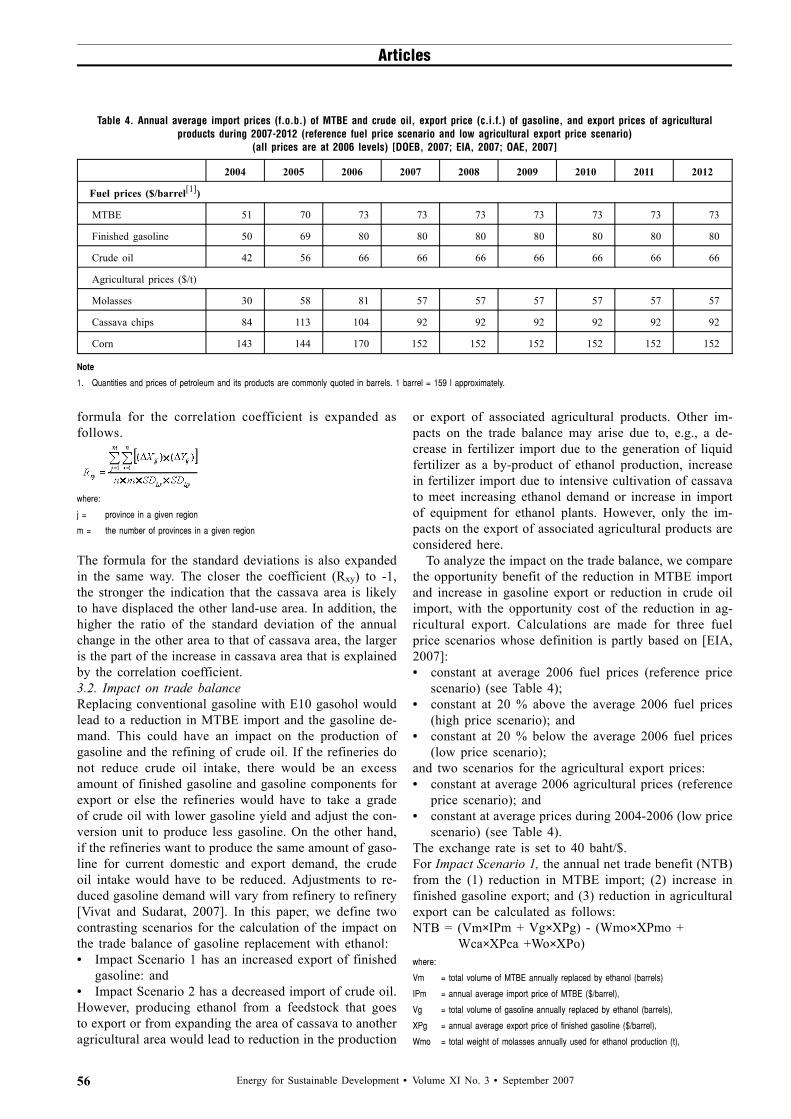
To analyze the impact on the trade balance, we comparethe opportunity benefit of the reduction in MTBE importand increase in gasoline export or reduction in crude oilimport, with the opportunity cost of the reduction in ag-ricultural export. Calculations are made for three fuelprice scenarios whose definition is partly based on [EIA,2007]:• constant at average 2006 fuel prices (reference price

scenario) (see Table 4);• constant at 20 % above the average 2006 fuel prices

(high price scenario); and• constant at 20 % below the average 2006 fuel prices

(low price scenario);and two scenarios for the agricultural export prices:• constant at average 2006 agricultural prices (reference

price scenario); and• constant at average prices during 2004-2006 (low price

scenario) (see Table 4).The exchange rate is set to 40 baht/$.For Impact Scenario 1, the annual net trade benefit (NTB)from the (1) reduction in MTBE import; (2) increase infinished gasoline export; and (3) reduction in agriculturalexport can be calculated as follows:NTB = (Vm×IPm + Vg×XPg) - (Wmo×XPmo +

Wca×XPca +Wo×XPo)where:

Vm = total volume of MTBE annually replaced by ethanol (barrels)

IPm = annual average import price of MTBE ($/barrel),

Vg = total volume of gasoline annually replaced by ethanol (barrels),

XPg = annual average export price of finished gasoline ($/barrel),

Wmo = total weight of molasses annually used for ethanol production (t),

Table 4. Annual average import prices (f.o.b.) of MTBE and crude oil, export price (c.i.f.) of gasoline, and export prices of agriculturalproducts during 2007-2012 (reference fuel price scenario and low agricultural export price scenario)

(all prices are at 2006 levels) [DOEB, 2007; EIA, 2007; OAE, 2007]

2004 2005 2006 2007 2008 2009 2010 2011 2012

Fuel prices ($/barrel[1])

MTBE 51 70 73 73 73 73 73 73 73

Finished gasoline 50 69 80 80 80 80 80 80 80

Crude oil 42 56 66 66 66 66 66 66 66

Agricultural prices ($/t)

Molasses 30 58 81 57 57 57 57 57 57

Cassava chips 84 113 104 92 92 92 92 92 92

Corn 143 144 170 152 152 152 152 152 152

Note

1. Quantities and prices of petroleum and its products are commonly quoted in barrels. 1 barrel = 159 l approximately.


Articles

56

XPmo = annual average export price of molasses ($/t),

Wca = total equivalent weight of cassava chips annually used for ethanol production instead of export (t),

XPca = annual average export price of cassava chips ($/t),

Wo = annual decline in total equivalent weight of other agricultural product export as a result of ethanol production (t),

XPo = annual average export price of other agricultural product ($/t)

3.2.1. Opportunity benefitThe annual reduction in the import of MTBE and gasolineis estimated on the basis of the product of the volume ofethanol annually used to blend in the gasoline (10 % ofthe annual total demand of gasohol 95 and gasohol 91)and the volumes of MTBE and gasoline replaced by 1 lof ethanol, respectively.

The volume of gasoline replaced by 1 l of ethanol iscalculated on the basis of [UNFCCC, 2006a]:

Rg = FCg − (FCgh × X)

FCgh − (FCgh × X)where

Rg = volume of gasoline displaced by 1 l of ethanol when ethanol is blended in gaso-line (l)

FCgh = fuel consumption of gasohol (l/km)

FCg = fuel consumption of gasoline (l/km)

X = blend of gasoline in gasohol (0.8 ≤ X ≤ 1)

The fuel efficiencies of the different gasoline grades areestimated on the basis of their relative heating values. InThailand, the specification of ULG 95 is set to containMTBE between 5.5 and 11 % by volume [DEDE, 2005].We assume ULG 95 contains 6 % MTBE and 94 % ULG91 by volume, while gasohol 95 contains 10 % ethanoland 90 % octane-91-based gasoline by volume. The highheating values used for non-MTBE blended conventionalgasoline with 91-octane number, MTBE, and ethanol aregiven in Table 5 [USEPA, 2007; Chevron, 2007]. Thisleads to the high heating values for ULG 95 and E10gasohol 95 (Table 5). Thus, the fuel efficiency of E10gasohol 95 is estimated to be 2 % lower than that ofULG 95.

ULG 91 does not contain MTBE while gasohol 91 con-tains 90 % octane-88-based gasoline and 10 % ethanol byvolume. The heating value of gasohol 91 is estimated at30.6 MJ/l (Table 5). Thus, the fuel efficiency of E10 gaso-hol 91 is estimated to be 3 % lower than that of ULG 91.

From the equation above, for ULG 95, 1 l of ethanol

in E10 gasohol 95 substitutes 0.8 l gasoline. Thus, 1 l ofethanol in E10 gasohol 95 replaces 0.6 l of MTBE and0.2 l of other gasoline components. For ULG 91, 1 l ofethanol in E10 gasohol 91 replaces 0.7 l of gasoline.

For Impact Scenario 2, the NTB from the reduction inMTBE and crude oil import and the reduction in agricul-tural export can be calculated as follows:NTB = (Vm×IPm + Vco×IPco) - (Wmo×XPmo +

Wca×XPca +Wo×XPo)where:

Vco = total volume of crude oil intake annually reduced due to the replacement of gasoline by ethanol, leading to lower gasoline demand (barrels),

IPco = annual average import price of crude oil ($/barrel), other terms being the same as before.

The annual reduction in the import of crude oil is calcu-lated as the product of the total volume of gasoline an-nually replaced by ethanol and the reduction in crude oilintake/l gasoline replaced.

Given a gasoline yield at 20-25 % [Vivat and Sudarat,2007], a lower demand for gasoline by 1 l would reducethe crude oil intake by 5 l. But that would also lead to alower production of other finished refinery products. Aconservative assumption is used: the reduction in crudeoil intake due to reduced gasoline demand is estimatedon the basis of the heating values of crude oil and gasolineat 38.8 and 31.6 MJ/l, respectively [Vivat and Sudarat,2007; USEPA, 2007].3.2.2. Opportunity costThe reductions in molasses and cassava chip exports areestimated on the basis of the ethanol demand given inFigure 3 and ethanol yields of 250 and 143 l/t of molassesand fresh cassava, respectively. 1 t of cassava chips isproduced from 2.1 t of fresh cassava [OAE, 2006].

On the basis of the result of the correlation analysis ofhistorical land-use change, the major crops that are likelyto be replaced by cassava are corn in the northeastern partand rice in the eastern part. Since the potential for ex-panding cassava cultivation on cropland used for corn inthe northeastern part is largest, and since corn is mainlyproduced as animal feed, it is assumed that cassava cul-tivation expands on cropland used for corn. The reductionin export of other agricultural products is therefore limitedto corn export reduction. The annual yield of corn duringthe period 2006-2012 is set to be constant at 3.7 t/ha.3.3. Self-sufficiency of gasoline andcassava/molasses/cornReplacing conventional gasoline with gasohol would leadto an increased domestic production of gasoline based ondomestic resources (domestic crude oil and ethanol) orless dependence on imported crude oil. However, in-creased ethanol production will, as described above, leadto reduced domestic production of cassava, molasses andcorn for food or feed purposes. A self-sufficiency rate in-dicator is defined as the ratio of domestic production todomestic consumption, following [Matsuda and Kubota,1989]. The indicator is used to assess the impact of re-placing conventional gasoline with gasohol on the self-sufficiency of gasoline, cassava, molasses and corn.

Annual average self-sufficiency rate of gasoline

Table 5. High heating values of gasoline and gasoline components

Gasoline and gasoline components High heating values(MJ/l)

Octane-91 non-MTBE blended conventional gasoline (ULG 91)

31.6

MTBE 26.1

Ethanol 21.2

ULG 95 31.3

E10 gasohol 95 30.6

E10 gasohol 91 30.6


Articles

57

(including conventional gasoline and gasohol) (SSg):

SSg = PgCg

where:

Pg = annual domestic production of gasoline based on domestic resources

(conventional gasoline equivalent-Ml)

Cg = average annual domestic consumption of gasoline

(conventional gasoline equivalent-Ml)

Annual average self-sufficiency rate of cassava for foodand feed (SSca):

SSca = PcaCca

where:

Pca = annual domestic production of fresh cassava for food and feed (Mt)

Cca = annual domestic consumption of fresh cassava (Mt)

The self-sufficiency rates of molasses and corn are calcu-lated in the same way as for cassava. To distinguish theimpact of the ethanol program on self-sufficiency rates ofgasoline, cassava, and corn for the period 2006-2012, an-nual domestic consumption of all the products over theperiod is set constant at the average values during 2000-2005. The annual average domestic consumption of gaso-line during 2000-2005 was 7,250 conventional gasoline-equivalent Ml [EPPO, 2007], while that of corn was 3.6Mt/yr [OAE, 2006]. The annual average domestic con-sumption of cassava and molasses during 2000-2005 ispresented in Tables 2 and 3, respectively. The annual pro-duction of gasoline based on domestic resources over theperiod is calculated as the sum of the average domesticproduction of gasoline based on domestic crude oil during2000-2005 (820 Ml) [EPPO, 2007] and the annual in-creased domestic production of gasoline based on ethanol.The domestic annual production of gasoline based on do-mestic crude oil is calculated from the product of the self-sufficiency of crude oil and the total domestic productionof gasoline based on total crude oil. The amount of in-creased domestic production of gasoline-equivalent fuelfrom ethanol is based on the fact that 1 l of ethanol cor-responds to 0.8 and 0.7 l of gasoline for ULG 95 andULG 91, respectively. The annual domestic production ofcassava and molasses (for non-fuel purposes) over the pe-riod is calculated by deducting the amount of the cassavaand molasses required for ethanol production from the av-erage total production during 2000-2005. The domesticannual production of corn for food/feed purposes is simi-larly calculated by deducting the reduction in the produc-tion due to cassava area expansion from the average totalproduction during 2000-2005.3.4. GHG emissionsThe annual reduction of GHG emissions due to the re-placement of conventional gasoline with gasohol is esti-mated from the difference between the baseline emissionsand the emissions from the ethanol program. The emis-sions due to land-use change are assumed negligible onthe basis that cassava area expansion is likely to take placemainly on corn area and not likely to cause significantdeforestation (See Section 4.1, “Land-use change im-pact”).

The baseline scenario assumes that emissions occurfrom conventional gasoline to be substituted by ethanol,taking into account the difference in fuel efficiency be-tween conventional gasoline and gasohol. Thus, the base-line emissions are calculated from the product of thelife-cycle GHG emissions of conventional gasoline andthe total volume of gasoline replaced by ethanol annually.The total life-cycle (well-to-wheels) GHG emission factorfor gasoline used in Thailand is set to 2.4 kgCO2e/l, basedon [Thu Lan et al., 2006; UNFCCC, 2006a]. The same valueis used for MTBE, although it has been estimated to behigher [UNFCCC, 2006a]. The annual demand for ethanolcorresponds to 10 % of the total volume of projected annualgasohol demand. The volume of gasoline replaced by 1 l ofethanol is calculated in the same way as in Section 3.2.

The program emissions are estimated on the basis ofthe product of the life-cycle emissions of ethanol and thetotal volume of annual demand for ethanol. The annualreduction in GHG emissions from replacing conventionalgasoline with gasohol is calculated as follows:

Annual reduction of GHG emissions (RE):RE = Eg× Rg -(Ee-m×De-m + Ee-ca×De-ca)where:

Eg = life-cycle GHG emissions of gasoline (tCO2e/l of gasoline)

Rg = total volume of 95-octane and 91-octane gasoline replaced by ethanol annually (Ml of gasoline)

Ee-m = life-cycle GHG emissions of ethanol produced from molasses (tCO2e/l of ethanol)

De-m = total volume of annual demand for ethanol produced from molasses (Ml of ethanol)

Ee-ca = life-cycle GHG emissions of ethanol produced from cassava (tCO2e/l of ethanol)

De-ca = total volume of annual demand for ethanol from cassava (Ml of ethanol)

The life-cycle emission factor for ethanol from molassesis set on the basis of the emission factor for sugarcaneproduction and ethanol production from sugarcane in Bra-zil (18 and 4 kgCO2e/t of sugarcane, respectively)[Macedo et al., 2003]. The life-cycle emissions from sug-arcane production include the emissions from the cultiva-tion and transportation of sugarcane and the productionof agricultural inputs such as fertilizers for sugarcane pro-duction. The allocation of emissions from sugarcane pro-duction between molasses and raw sugar is based on theamount of actual sugar content in these two processstreams, since the major reason for growing sugarcane isto obtain sugar and the sugar content also correlates di-rectly with ethanol output [UNFCCC, 2006a].

Emo = SmoRmo × Smo + Rrs × Sr s

× Esd

where:

Emo = life-cycle GHG emissions of molasses (kgCO2e/t of molasses)

Rmo = molasses recovery rate from sugarcane (t of molasses/t of sugarcane)

Smo = sugar content of molasses (t of sugar/t of molasses)

Rrs = raw sugar recovery rate from sugarcane (t of raw sugar/t of sugarcane)

Srs = sugar content of raw sugar (t of sugar/t of raw sugar)

Esc = life-cycle GHG emissions of sugarcane (kgCO2e/t of sugarcane)

1 t of cane produces 0.1 t of raw sugar and 0.047 t ofmolasses [OAE, 2006]. The sugar content of raw sugarand molasses is 80 % and 45 %, respectively [UNFCCC,


Articles

58

2005]. As a result, the emission factor for ethanolproduced from molasses is estimated at 0.4 kgCO2e/l. Forethanol produced from cassava in Thailand, the emissionfactor has been estimated at 0.96 kgCO2e/l [Thu Lan etal., 2006].3.5. Cost of replacing gasoline with gasoholThe cost of replacing conventional gasoline with gasoholis defined as the additional cost of supplying gasoholcompared to that of supplying conventional gasoline atthe gasoline station. The transportation and distributioncosts of conventional gasoline and gasohol are assumedto be the same. Consequently, the cost of replacing con-ventional gasoline with gasohol is the additional cost ofproducing gasohol in place of conventional gasoline.

The additional cost of producing gasohol during 2005-2006 is calculated from the difference between the actualprices of conventional gasoline and gasohol of the sameoctane number (monthly ex-refinery prices, i.e., the pricesat the refinery gate before taxes and marketing margin)[EPPO, 2007]. The ex-refinery prices of conventionalgasoline (ULG 95 and ULG 91) are not determined on acost-plus basis but are set equal to the mean price of ULG95 at the spot market Platt in Singapore plus a premium.The ex-refinery prices of gasohol 95 and gasohol 91 areset at the sum of 90 % of the ex-refinery price of ULG95 and ULG 91, respectively, plus 1 $/barrel, and 10 %of the price of ethanol [EPPO, 2007]. Thus, the differencebetween the ex-refinery prices of conventional gasolineand gasohol reflects the additional costs of producinggasohol. Since the consumption of gasohol 91 was rela-tively small compared to that of gasohol 95, the cost ofgasoline substitution during 2005-2006 is based on onlyoctane-95 ULG and gasohol.

Figure 5 shows that the ex-refinery price of ULG 95has mostly been lower than that of gasohol 95 per equiva-lent l of gasohol 95. This is due to the higher productioncost of ethanol and 91-octane base gasoline compared tothat of ULG 95. Since gasohol 95 is set to have 2 %lower fuel efficiency than gasoline, 1 l of ULG 95 cor-responds to 1.02 l of gasohol 95.

The annual average cost of replacing conventional

gasoline with gasohol (per tCO2e of GHG emissionreduction) is calculated from the total annual cost of re-placing gasoline with gasohol per tCO2e annual reductionof GHG emissions as follows.

Annual average cost of gasoline substitution (Cgs) dur-ing 2005-2006 ($/tCO2e):

Where:

i = month (1, 2, ..., 12)

Pgh95i = monthly average ex-refinery price of gasohol 95 ($/l of gasohol 95)

Pgh91i = monthly average ex-refinery price of gasohol 91 ($/l of gasohol 91)

Pg95i = monthly average ex-refinery price of ULG 95 ($/l of ULG 95)

Pg91i = monthly average ex-refinery price of ULG 91 ($/l of ULG 91)

Cgh95i = monthly consumption of gasohol 95 (Ml)

Cgh91i = monthly consumption of gasohol 91 (Ml)

RE = annual reduction of GHG emissions (MtCO2e)(taken from the previous section)

The cost of replacing gasoline with gasohol during 2007-2012 is calculated in the same way as during 2005-2006but based on the difference between the future annualaverage ex-refinery prices of ULG and gasohol of thesame octane number. We assume that the prices of gaso-line at the spot market in Singapore and the prices ofethanol during 2007-2012 are constant at the average val-ues in 2006. The annual average ex-refinery price of ULG95 and gasohol 95 is set to be constant at the averagevalues in 2006: 0.45 $/l of ULG 95 and 0.46 $/l of gaso-hol 95. The annual average ex-refinery price of ULG 91is set to be 0.013 $/l lower than that of ULG 95 and theannual average ex-refinery price of gasohol 91 is set tobe 0.008 $/l lower than that of gasohol 95, the averagedifference in the values in 2006 [EPPO, 2007]. From2008, it is assumed that there would be no sale of ULG95 and thus there would be no cost of replacing ULG 95with gasohol 95 (the first term in the above equation).3.6. Tax revenue forgone in implementing the ethanolprogramThe government has subsidized the ethanol program bysetting the retail price of gasohol at the gasoline stations

Figure 5. Monthly average ex-refinery price of ULG 95 and gasohol 95 during 2005-2006 [EPPO, 2007]


Articles

59

lower than the retail price of conventional gasoline. Thestructure of the retail prices of conventional gasoline andgasohol is the sum of the ex-refinery price, excise tax,municipal tax, Oil Fund tax, Energy Conservation Promo-tion Fund tax, VAT, and marketing margin. The retail priceof gasohol is set lower than that of conventional gasolineby the exemption of tax for fuel ethanol production andthe reduction of tax for ethanol blended in gasoline, in-cluding the reduction of excise and municipal tax and oftax collected for the Oil Fund and Energy ConservationPromotion Fund. The retail price difference was initiallyset at 0.013 $/l in 2004, but has later increased to 0.025and 0.038 $/l (November 2006). The tax revenue forgonein implementing the ethanol program is based on the sumof the difference between all the taxes on conventionalgasoline and on gasohol. The tax revenue forgone in im-plementing the program during 2005-2006 is estimated onbasis of the monthly average of all taxes on conventionalgasoline and gasohol. Figure 6 shows the contributions ofdifferent tax reductions for gasohol 95 compared withULG 95 during January 2004-October 2006.

The tax revenue forgone in implementing the programis calculated as follows:

Annual average tax revenue forgone (TRF) during2005-2006 ($/tCO2e):

where:

i = month (1, ..., 12)

Tg95i = total monthly average of all taxes on ULG 95 ($/l of ULG 95)

Tgh95i = total monthly average of all taxes on gasohol 95 ($/l of gasohol 95)

Tei = monthly average tax exemption for fuel ethanol production ($/l of ethanol)= 0.013 $/l

Cgh95i = annual consumption of gasohol 95 (Ml)

RE = annual reduction of GHG emissions (MtCO2e)

The tax revenue forgone in implementing the ethanol pro-gram during 2007-2012 is calculated from the sum of the

fuel retail price gap at 0.038 $/l of ULG and gasohol forboth octane-95 and octane-91 [EPPO, 2007], as it cur-rently is, and the difference between the annual averageex-refinery prices of gasohol and ULG of both octane-95and octane-91 (Section 3.5). A similar equation to theabove equation is applicable to 91-octane gasoline andgasohol. From 2008, it is assumed that there would be nosale of ULG 95 and that the retail price of gasohol 95would no longer be subsidized and there would thus beno tax revenue forgone in replacing 95-octane gasolinewith gasohol 95.

4. Results4.1. Land-use change impactThe result from the correlation analysis indicates that thehistorical increase in cassava area in the northeastern andeastern provinces has most likely resulted in a decreasein different combinations of a few of the following areas:corn area, rice fields, pasture, idle area, non-crop areas,non-agricultural area and forests (Table 6).

For the seven northeastern provinces as a whole, thehistorical increase in cassava area is most strongly linkedto a decrease in corn area (strongest correlation), pastureand non-crop area (Table 6). The standard deviation ofthe ratio of change in corn cultivation to change in cassavacultivation suggests in fact that close to 100 % of theincrease in cassava area is explained by the reduction incorn area. Besides, the other two areas currently availableare much smaller than the corn area. This altogether in-dicates that cassava cultivation has expanded mainly onland previously used for corn cultivation and only to alimited extent on pasture and non-crop area.

For the five eastern provinces as a whole, the resultindicates that cassava cultivation has likely expanded onmainly rice fields and only to a small extent on pastures.

The indication from the correlation analysis – that theexpansion of cassava cultivation is likely to take place onland used for corn and rice – is also consistent with thesurvey of farmers’ land-use plan and forecast for the area

Figure 6. The amount of tax subsidies for ethanol compared with gasoline during January 2004-October 2006


Articles

60

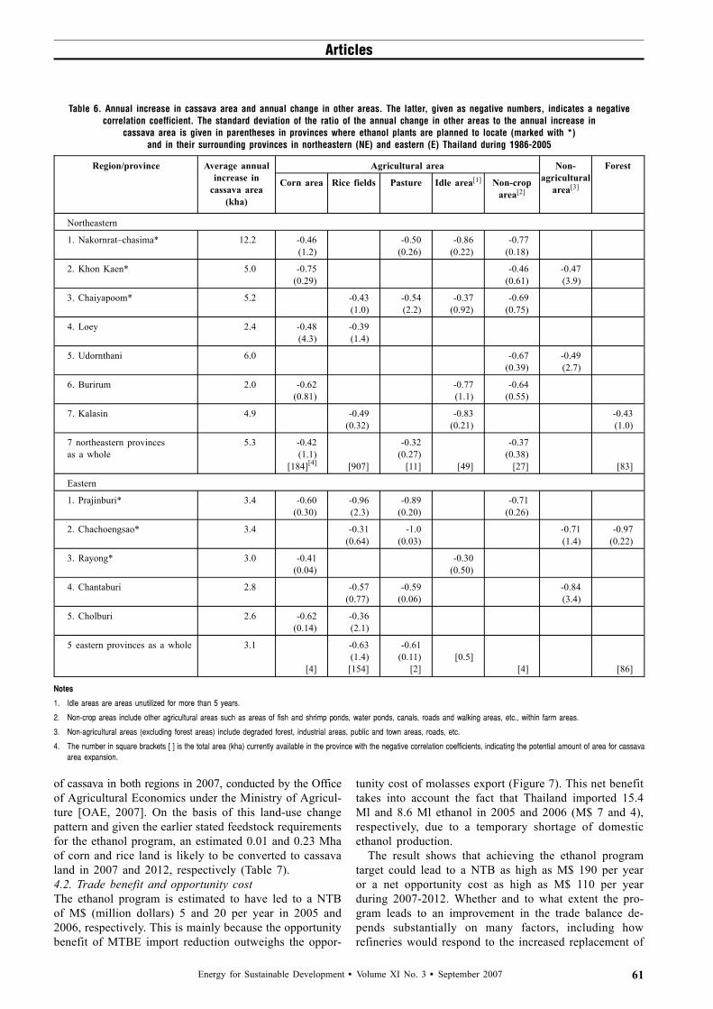
of cassava in both regions in 2007, conducted by the Officeof Agricultural Economics under the Ministry of Agricul-ture [OAE, 2007]. On the basis of this land-use changepattern and given the earlier stated feedstock requirementsfor the ethanol program, an estimated 0.01 and 0.23 Mhaof corn and rice land is likely to be converted to cassavaland in 2007 and 2012, respectively (Table 7).4.2. Trade benefit and opportunity costThe ethanol program is estimated to have led to a NTBof M$ (million dollars) 5 and 20 per year in 2005 and2006, respectively. This is mainly because the opportunitybenefit of MTBE import reduction outweighs the oppor-

tunity cost of molasses export (Figure 7). This net benefittakes into account the fact that Thailand imported 15.4Ml and 8.6 Ml ethanol in 2005 and 2006 (M$ 7 and 4),respectively, due to a temporary shortage of domesticethanol production.

The result shows that achieving the ethanol programtarget could lead to a NTB as high as M$ 190 per yearor a net opportunity cost as high as M$ 110 per yearduring 2007-2012. Whether and to what extent the pro-gram leads to an improvement in the trade balance de-pends substantially on many factors, including howrefineries would respond to the increased replacement of

Table 6. Annual increase in cassava area and annual change in other areas. The latter, given as negative numbers, indicates a negativecorrelation coefficient. The standard deviation of the ratio of the annual change in other areas to the annual increase in

cassava area is given in parentheses in provinces where ethanol plants are planned to locate (marked with *)and in their surrounding provinces in northeastern (NE) and eastern (E) Thailand during 1986-2005

Region/province Average annualincrease in

cassava area(kha)

Agricultural area Non-agricultural

area[3]

Forest

Corn area Rice fields Pasture Idle area[1] Non-croparea[2]

Northeastern

1. Nakornrat–chasima* 12.2 -0.46(1.2)

-0.50(0.26)

-0.86(0.22)

-0.77(0.18)

2. Khon Kaen* 5.0 -0.75(0.29)

-0.46(0.61)

-0.47(3.9)

3. Chaiyapoom* 5.2 -0.43(1.0)

-0.54(2.2)

-0.37(0.92)

-0.69(0.75)

4. Loey 2.4 -0.48(4.3)

-0.39(1.4)

5. Udornthani 6.0 -0.67(0.39)

-0.49(2.7)

6. Burirum 2.0 -0.62(0.81)

-0.77(1.1)

-0.64(0.55)

7. Kalasin 4.9 -0.49(0.32)

-0.83(0.21)

-0.43(1.0)

7 northeastern provincesas a whole

5.3 -0.42(1.1)

[184][4] [907]

-0.32(0.27)

[11] [49]

-0.37(0.38)

[27] [83]

Eastern

1. Prajinburi* 3.4 -0.60(0.30)

-0.96(2.3)

-0.89(0.20)

-0.71(0.26)

2. Chachoengsao* 3.4 -0.31(0.64)

-1.0(0.03)

-0.71(1.4)

-0.97(0.22)

3. Rayong* 3.0 -0.41(0.04)

-0.30(0.50)

4. Chantaburi 2.8 -0.57(0.77)

-0.59(0.06)

-0.84(3.4)

5. Cholburi 2.6 -0.62(0.14)

-0.36(2.1)

5 eastern provinces as a whole 3.1

[4]

-0.63(1.4)[154]

-0.61(0.11)

[2][0.5]

[4] [86]

Notes

1. Idle areas are areas unutilized for more than 5 years.

2. Non-crop areas include other agricultural areas such as areas of fish and shrimp ponds, water ponds, canals, roads and walking areas, etc., within farm areas.

3. Non-agricultural areas (excluding forest areas) include degraded forest, industrial areas, public and town areas, roads, etc.

4. The number in square brackets [ ] is the total area (kha) currently available in the province with the negative correlation coefficients, indicating the potential amount of area for cassavaarea expansion.


Articles

61

gasoline with ethanol (export more gasoline or reducecrude oil import), share of cassava supply from exportreduction vs. production increase, as well as import andexport prices of fuel and agricultural products.4.2.1. Scenario 1, where refineries would export moregasoline (see Figures 7 and 8)The outcome of the ethanol program in this scenario isestimated to range from a NTB of M$ 190 per year to anet opportunity cost of M$ 45 per year. If all the cassavasupply for ethanol production were from cassava area ex-pansion replacing corn area, there would be an improve-ment in trade balance for all scenarios of agricultural andfuel prices. On the other hand, if all the cassava supplyfor ethanol production were from export reductions, therewould be lower NTBs for all prices scenarios. This is dueto the fact that the opportunity cost of reducing the export

Table 7. The accumulated cassava area expansion required (the caseof 0 % of cassava supply from export reductions) and major areas

that are likely to be replaced by cassava

Accumulated cassava areaexpansion (Mha)

Major areas likely to bereplaced

2005 - -

2006 - -

2007 0.01

Area of corn and rice fields

2008 0.03

2009 0.04

2010 0.09

2011 0.15

2012 0.23

Figure 7. Opportunity benefit and cost for Scenario 1: export more gasoline (reference fuel prices and low agricultural export prices scenario)

Figure 8. Net trade benefit for Scenario 1 (export more gasoline) with different scenarios of agricultural and fuel prices at 0 and 100 % of cassavasupply from export reduction


Articles

62

of cassava chips outweighs the opportunity cost of re-ducing the export of corn.4.2.2. Scenario 2, where refineries would reduce crudeoil import (Figure 9)Compared to Scenario 1, where refineries would exportmore gasoline, this scenario is estimated to yield lessNTBs for all the cases of cassava supply. The outcomeranges from a NTB of M$ 95 per year to a net opportunitycost of M$ 110 per year. This is partly due to the factthat the import price of crude oil is less than the exportprice of gasoline per unit volume.4.3. Self-sufficiency of gasoline, cassava, corn, andmolassesWithout the ethanol program, the average self-sufficiency

rate of gasoline during 2000-2005 was 11 % while thoseof fresh cassava, corn, and molasses were 425 %, 118 %and 193 %, respectively (Figure 10). With the ethanolprogram, the self-sufficiency rate of gasoline increases to13 % in 2006 and to 21 % in 2012. On the other hand,the self-sufficiency rate of molasses would decrease to100 % in 2012. To what extent the self-sufficiency ratesof cassava and corn decrease depends on the shares ofthe supply of cassava from export reduction and area ex-pansion replacing corn area.

If all cassava supply for ethanol production were fromexport reduction, the self-sufficiency rate of cassavawould decrease to 332 % in 2012. On the other hand, ifall the cassava supply were from cassava area expansion

Figure 9. Net trade benefit for Scenario 2 (reduce crude oil import) with different scenarios of agricultural and fuel prices at 0 and 100 % of cassavasupply from export reduction

Figure 10. Self-sufficiency rates of fresh cassava, molasses, corn and gasoline during 2006-2012 with the ethanol program (for 2005*, the rates arethe average values during 2000-2005) at 0 and 100 % of cassava supply from export reduction


Articles

63

replacing corn area, the self-sufficiency rate of corn woulddecrease to 95 % in 2012.

The result shows that at the present program targetThailand would still be self-sufficient in associated foodcrops for food/feed purposes with the self-sufficiencyrates of about 100 % or higher.4.4. GHG emission reduction, cost of gasolinesubstitution, and tax revenue forgone in implementingthe programMeeting the program targets reduces GHG emissions by4.0 Mt during 2005-2012 (see Table 8), corresponding to2 % of the country’s total energy-related CO2 emissionsin 2004 [EIA, 2006; IEA, 2006b].

The annual average gasoline substitution cost during2005-2012 is estimated at 27-194 $/tCO2e. The averagecost of gasoline substitution is estimated at 69 $/tCO2e in2005 and increases to 177 $/tCO2e in 2006 mainly dueto the increased difference between the ex-refinery pricesof gasohol 95 and ULG 95. The average cost is expectedto increase to 194 $/tCO2e in 2007 due to the increasedreplacement of ULG 91 with gasohol 91 and relative in-creased use of ethanol from cassava. The average cost ofgasoline substitution is expected to decrease to 27 $/tCO2ein 2008, when there would be no sale of ULG 95 and nofurther cost of replacing ULG 95 with gasohol 95.

The tax revenue forgone in implementing the programis estimated at 281 $/tCO2e in 2005 and increases to 370$/tCO2e in 2006 due to the increased difference betweenthe ex-refinery prices of gasohol 95 and ULG 95 and theincreased retail price gap in 2006 compared with that in2005. The tax revenue forgone in 2005 and 2006 corre-sponds to about four times and twice the average cost ofgasoline substitution in the two years, respectively. During2007-2012, the tax revenue forgone is expected to showthe same trend as the average cost of gasoline substitutionand correspond to twice to thrice the average cost of gaso-line substitution in the respective years.

5. Prospects for CO2 abatement by the nationalethanol programSo far, there have been a few proposed CDM projects on

biofuel production for blending with fossil fuels, includ-ing projects on the production of fuel ethanol, palm bio-diesel and sunflower biodiesel in Thailand, and theproduction of biodiesel from non-edible oil crops in India.However, the methodologies developed for these projectshave not yet been approved. There are a number of issuesthat still need to be addressed before the methodologiescan be approved, including the estimation of a baselineand leakage emissions, estimation and monitoring ofemission reductions, and the issue of double-counting[UNFCCC, 2006c].5.1. Baseline and additionalityAccording to the modalities and procedures for the CDM,relevant national or sectoral policies and circumstancesshall be taken into account in the identification of a base-line and demonstration of additionality [UNFCCC, 2005].Under Thailand’s ethanol program, the government sup-port has been dynamic. The government has set the retailprice of gasohol at the gasoline stations lower than theretail price of conventional gasoline by the exemption oftax for fuel ethanol production and the reduction of taxfor ethanol blended in gasoline in order to boost the de-mand for gasohol and supply of fuel ethanol. In responseto fluctuating crude oil prices and ethanol feedstock price,the government has several times adjusted the retail pricegap and the level of tax reductions as shown in Figure 5.In addition, during the end of 2005 and the beginning of2006, the demand for ethanol outweighed its supply andthe government responded by importing a certain amountof ethanol. On the other hand, since the end of 2006, thegovernment has postponed an earlier target of replacingULG 95 with gasohol 95 from January 1, 2007, so thesupply of ethanol has outweighed the demand for it. Forthe only CDM ethanol project in Thailand proposed sofar, a proposed methodology requires that the relevant na-tional ethanol market is production-constrained or a lackof supply of ethanol is the limiting factor for the ethanoluse and that there does not exist an effectively enforcedmandate on the use of ethanol [UNFCCC, 2006a]. Thus,in the case of Thailand, the proposed methodology is notapplicable.

Table 8. GHG emission reduction, the cost of gasoline substitution, and the tax revenue forgone in implementing the program(all costs are normalized at 2006 values)

Ethanol demand(Ml)

Annual GHGreduction

(Mt)

Total cost ofgasoline

substitution (M$)

Average cost ofgasoline

substitution($/tCO2e)

Total tax revenue forgone

(M$)

Tax revenueforgone per unit

of GHG reduction($/tCO2e)

2004 6 0.01 NA NA 1 100

2005 67 0.1 7 69 29 281

2006 129 0.2 35 177 72 370

2007 217 0.3 60 194 140 452

2008 326 0.5 12 27 26 58

2009 424 0.6 39 70 85 152

2010 551 0.7 75 114 163 249

2011 717 0.8 122 157 267 344

2012 913 0.9 179 194 391 425


Articles

64

In fact, after the CDM project on ethanol productionin Thailand was proposed in 2004, the number of ethanolproduction plants in operation in Thailand has increased(see Table 2) and even more ethanol plants are scheduledand planned for operation. This indicates that with thegovernment policy and support, ethanol production plantsare economically feasible without the CDM, and thus theproposed CDM project would not necessarily lead to theuse of ethanol: the additionality can be questioned.5.2. Monitoring methodology and the issue ofdouble-countingAlthough there might be cases where no significantchange in the government support and responses to chang-ing conditions occurs, the methodology for these CDMproject activities still needs to ensure that double-countingof emission reductions does not occur at the productionand use phase – as well as of project activities using bio-fuels domestically and exporting them. Thus, monitoringof different uses and export of biofuels produced fromthe project activities is needed. Although imposing a con-tractual obligation with identified biofuel consumers andtaking into account biofuel sales to unidentified consum-ers was suggested to avoid double-counting [UNFCCC,2006d], monitoring different uses of biofuels producedfrom each project activity becomes more complicated, forinstance, in cases where there are various gasoline grades,various ratios of biofuels in the blend, and other biofuelproduction plants.

In fact, Thailand’s ethanol program illustrates that un-der dynamic government support, it may not be possibleto identify and claim additionality of CDM projects onbiofuel production for blending with fossil fuels. On theother hand, compared to the proposed CDM projects onbiofuels, the national ethanol program could in itself bean example of a suitable programmatic approach, avoid theproblems of double-counting and also have other advan-tages.

A national program might be credited for emission re-ductions through CDM or other mechanisms. A nationalprogram as the basis for carbon credits would also requireadequate baseline and monitoring procedures. However,the baseline could be established more easily, and in amore transparent manner. The national baseline scenariofor the national program would be the scenario withoutthe government support. For instance, before the govern-ment’s ethanol program and support by setting the retailprice of gasohol lower than conventional gasoline startedin 2004, there were almost no sales of gasohol. Withthe ethanol program there is now a substantial amountof gasohol use and sales. This is the program scenario.The difference is the cumulative amount of gasohol salesfrom the start of the program; this is the amount of emis-sion reductions as a result of the government support.

In addition, the national program could allow for easiermonitoring. Emission reductions are monitored at the useof biofuels based on the well-established national statis-tics of different total biofuel-blended gasoline sales andbiofuel import as partly illustrated in Section 3.4. Thus,double-counting of emission reductions could be avoided.

5.3. Other advantages of the ethanol program1. The program is derived from and reflects the country’s

development priorities of reducing dependence oncrude oil and fuel import and trade deficit, enhancingthe agricultural sector, and reducing atmospheric emis-sions. The ethanol program could have more substantialdevelopment impacts in addition to GHG emission re-ductions than the proposed CDM projects on biofuels.

2. The ethanol program could lead to annual averageemission reductions of 0.5 MtCO2e compared with0.05 MtCO2e of the only CDM ethanol project in Thai-land proposed so far [UNFCCC, 2005]. Till the endof 2012, the ethanol program is expected to lead to atotal emission reduction of 4.0 MtCO2e compared with0.2 MtCO2e of the CDM ethanol project in Thailand.So, the ethanol program allows for large volumes ofemission reductions to take place.

3. Although the estimated average cost of replacing gaso-line with gasohol is substantially higher than the priceof project-based certified emission reductions (CERs),at 6-24 $/tCO2e transacted during 2006 [Capoor andAmbrosi, 2006], the estimated average cost is lowerthan or within the lower range of the marginal CO2abatement cost for the road transportation sector of70-350 Euro/tCO2e [Blok et al., 2001] and is relativelylow compared with estimates of the cost of substitut-ing biofuels for fossil fuels in Europe, at 230-2,000Euro/tCO2e [Ryan et al., 2006]. In addition, taking intoaccount the easier monitoring of emission reductionsof the national program compared to the proposedCDM projects, the transaction cost per tCO2e of theprogram might be less than that of the project-basedemission reduction activities.

However, it should be noted that the government currentlysubsidizes the ethanol program through reductions oftaxes for gasohol, which serves to lower the retail priceof gasohol compared to gasoline. This directly benefitscar users. The distribution of the benefits to other relevantstakeholders such as ethanol producers and farmers whocultivate feedstock crops, and also the possibility of en-tailing an increased use of gasoline, should be considered.

6. Conclusions and policy implicationsIn this paper, we quantify the impacts of achieving thetargets set in the ethanol program in Thailand. However,we do not analyze whether and to what extent the targetscould be achieved. We find that achieving the currentethanol program target of replacing all non-ethanol refor-mulated gasoline with E10 gasohol in 2012 leads to asignificant improvement in gasoline self-sufficiency anda significant reduction of GHG emissions. Whether andto what extent the program leads to an improvement inthe trade balance depends substantially on the future fuelimport and export prices and agricultural export prices aswell as the shares of cassava supply from export reductionand cassava area expansion. It also depends on how re-fineries would respond to the increasing replacement ofgasoline with ethanol (export more gasoline or reducecrude oil import).


Articles

65

Achieving the ethanol target could lead to a significantreduction of self-sufficiency of molasses. To what extentthe self-sufficiency rates of cassava and corn decrease de-pends on to what extent the supply of cassava comes fromexport reduction vs. area expansion. Cassava area expan-sion has significantly taken place on areas of food cropsand not on forest area and an expansion of cassava areadue to the ethanol program would likely take place onland used for food crops – mainly corn but also rice. Theprogram target leads to a reduction in the self-sufficiencyof associated food crops but the rates would still be about100 % or higher. Thus, Thailand’s agricultural sectorshould be able to accommodate the present level of pro-gram target.

Compared to the proposed CDM projects on biofuelproduction for blending with fossil fuels, implementingnational programs on biofuels such as the ethanol programin Thailand could contribute significantly to abating GHGemissions in the transportation sector and could avoid theproblems of double-counting. The gasoline substitutioncost is high compared with the price of project-basedCERs traded during 2006 but relatively low comparedwith the estimates of the cost of substituting fossil fuelswith biofuels in Europe [Ryan et al., 2006]. The tax reve-nue forgone in implementing the ethanol program is 2-4times this gasoline substitution cost, because of the lowerprice of gasohol set by the government.

Acknowledgements

The authors thank Pornpun Hensawang at the Office of Agricultural Economics under theThai Ministry of Agriculture for providing valuable agricultural data, Christian Azar for hiscritical comments and useful advice, Paulina Essunger for critical review, and the SwedishEnergy Agency for financial support.

Notes

1. Octane-91 unleaded gasoline (ULG 91), octane-91 gasohol (gasohol 91), octane-95unleaded gasoline (ULG 95) and octane-95 gasohol (gasohol 95).

2. Based on regression analysis with the logarithm of the gasoline demand during 1998-2005 as the dependent variable [NESDB, 2006; EPPO 2007].

References

Bangchak (Bangchak Petroleum Public Company Ltd.), 2006. Gasohol 95 (in Thai), Bangkok,Thailand, www.bangchak.co.th.

Best, G., 2006. FAO Newsroom. FAO Sees Major Shift toward Bioenergy: Pressure Buildingfor Switch to Biofuels, www.fao.org.

Blok, K., De Jager, D., and Hendriks, C., 2001. Economic Evaluation of Sectoral EmissionReduction Objectives for Climate Change, summary report for policy-makers, ECOFYS En-ergy and Environment, AEA Technology, National Technical University of Athens,http://europa.eu.int/comm/environment/enveco/climate_change/sectoral_objectives.htm.

Browne, J., Sanhueza, E., Silsbe, E., Winkelman, S., and Zegras, C., 2005. Getting onTrack: Finding a Path for Transportation in the CDM, final report, International Institute forSustainable Development, Winnipeg, March.

Capoor, K., and Ambrosi, P., 2006. State and Trends of the Carbon Market 2006: Update(January 1-September 30, 2006), World Bank, Washington, DC.

Chevron, 2007. Oxygenated Gasolines and Fuel Economy: Energy Content of Gasoline,www.chevron.com.

Dalkmann, H., Bongardt, D., Sterk, W., Wittneben, B., and Baatz, C., 2006. Driving theClean Development Mechanism into a Sustainable Transport Future, Conference of Par-ties/Meeting of Parties (COP/MOP) side event, Nairobi, 12 November,http://regserver.unfccc.int/seors/file_storage/ke68gdbapf9219f.pdf.

DEDE (Department of Energy Development and Efficiency), 2005. Renewable Energy inThailand: Ethanol and Biodiesel, Ministry of Energy (MOE), Thailand.

DOEB (Department of Energy Business), 2007. Statistics, Ministry of Energy (MOE), Thai-land, www.doeb.go.th.

EIA (US Energy Information Administration), 2006. International Energy Annual 2004,www.eia.doe.gov/emeu/international.

EIA (US Energy Information Administration), 2007. Short Term Energy Outlook, January 9release, www.eia.doe.gov/emeu/steo/pub/jan07.pdf.

EPPO (Energy Policy and Planning Office), 2007. Energy Data Notebook Quarterly, EnergySituation in 2006, and Biofuel Reports, Ministry of Energy (MOE), Thailand, www.eppo.go.th.Figueres, C., 2005. Study on Programmatic CDM Project Activities: Eligibility, MethodologicalRequirements and Implementation, report prepared for the World Bank, International Institutefor Sustainable Development.FO Lichts, 2005. World Ethanol and Biofuels Report, No. 4, 25 October.Fulton, L., Howes, T., and Hardy, J., 2004. Biofuel for Transport: an International Perspective,International Energy Agency, Paris.Gowen, M.M., 1989. “Biofuel versus fossil fuel economics in developing countries: how greenis the pasture?”, Energy Policy, October, pp. 455-470.IEA (International Energy Agency), 2006a. World Energy Outlook 2006, International EnergyAgency, Paris, www.iea.org.IEA (International Energy Agency), 2006b. Key World Energy Statistics, 2006 edition, Inter-national Energy Agency, Paris, www.iea.org.Jackson, M., and Morales, M.M., 2004. “Fuel ethanol use: promising prospects for the fu-ture”, Renewable Energy for Development, Stockholm Environment Institute’s newsletter ofthe energy program, Vol. 17, No. 1, January.Macedo, I. de C., Leal, M.R.L.V., and da Silva, J.E.A.R., 2003. Greenhouse Gas Emissionsin the Production and Use of Ethanol in Brazil: Present Situation (2002), University of Campi-nas, Brazil.Matsuda, S., and Kubota, H., 1984. “The feasibility of fuel-alcohol programs in southeastAsia”, Biomass, 4, pp. 161-182.Moreira, J.R., and Goldemberg, J., 1999. “The alcohol program”, Energy Policy, 27, pp.229-245.Moore, S.D., and McCabe, P.G., 1999, Introduction to the Practice of Statistics, (3rd ed.),W.H. Freeman and Company, New York.NESDB (National Economic Social Development Board), 2006. Quarterly Gross DomesticProduct, Thailand, www.nesdb.go.th.OAE (Office of Agricultural Economics), 2006. Yearbook of Agricultural Data of Thailand (inThai), Ministry of Agriculture, Thailand, www.oae.go.th.OAE (Office of Agricultural Economics), 2007. The Result of the Forecast of Cassava Pro-duction Year 2007 (in Thai), Ministry of Agriculture, Thailand,www.oae.go.th/mis/Forecast/thai/situation/sit_t_8.htm.OCSB (Office of Cane and Sugar Board), 2007. Sugarcane and Sugar Economics Newsand Announcements (in Thai), Ministry of Industry, Thailand, www.ocsb.go.th.Ortiz, L., and Noronha, S., 2006. Agribusiness and Biofuels: an Explosive Mixture: Impactsof Monoculture Expansion on Bioenergy Production in Brazil, Friends of the Earth Brazil.PTTRTI (PTT Research and Technology Institute), 2007. Gasohol: Tests Conducted by PTTResearch and Technology Institute: Effects on Emission and Fuel Consumption, Bangkok,Thailand, www.pttplc.com.Rosillo-Calle, F., and Cortez, L., 1998. “Towards Proalcool 2: a review of the Brazilianbioethanol program”, Biomass and Bioenergy, 14(2), pp. 115-124.Ryan L., Convery, F., and Ferreira, S., 2006. “Stimulating the use of biofuels in the EuropeanUnion: implications for climate change policy”, Energy Policy, 34, pp. 3184-3194.Suksunthornsiri, P., Tia, W., and Limmechokchai, B., 2006. “Economy-wide impacts of policyon biofuel utilization in Thailand: an input-output analysis”, Proceedings of the World Re-newable Energy Congress IX, Florence, Italy, August.Thomas, V., and Kwong, A., 2001. “Ethanol as a lead replacement: phasing out leadedgasoline in Africa”, Energy Policy, 29, pp. 1133-1143.Thu Lan, T., Shabbir, H., and Garivait, S., 2006. “Assessing energy, environmental andeconomic performance of bio-ethanol in Thailand”, Proceedings of the International Confer-ence on Green and Sustainable Innovation, Chiengmai, Thailand, December.UNFCCC (United Nations Framework Convention on Climate Change), 2005. CDM ProjectDesign Document (PDD) of Khon Kaen Fuel Ethanol Project (NM0082),http://cdm.unfccc.int/UserManagement/FileStorage/FS_901804832.UNFCCC (United Nations Framework Convention on Climate Change), 2006a. CDM MethPanel. Draft Baseline Methodology: Production of Sugarcane-based Anhydrous Bio-ethanolfor Transportation Using Life Cycle Analysis (NM0082),http://cdm.unfccc.int/UserManagement/FileStorage/FS_130914325.UNFCCC (United Nations Framework Convention on Climate Change), 2006b. CDM Sta-tistics, http://cdm.unfccc.int/Statistics.UNFCCC (United Nations Framework Convention on Climate Change), 2006c. CDM SSCWG, Fifth Meeting Report, Annex 9, Request for Public Inputs on Biofuels,http://cdm.unfccc.int/Panels/ssc_wg/SSCWG05_repan_09_Recom_Call_Public_inputs.pdf.UNFCCC (United Nations Framework Convention on Climate Change), 2006d. CDM: MethPanel Recommendation to the Executive Board, F_CDM_NM0108-rev: Biodiesel Productionand Switching Fossil Fuels from Petro-diesel to Biodiesel in Transport Sector in AndhraPradesh, India, http://cdm.unfccc.int/UserManagement/FileStorage/CDMWF_OB8Q5Z4ES4AGQ5QB1BJ68ISOP57D4V.USEPA (US Environmental Protection Agency), 2007. Fuel Economy Impact Analysis ofReformulated Gasoline, www.epa.gov/orcdizux/rfgecon.htm.Vivat, W., and Sudarat, O., (Thai Oil Public Company Ltd., Commercial and Technical Plan-ning Divisions), 2007. Personal communication.


Articles

66

Documents

Amatayakul_2007_Energy-for-Sustainable-Development