Embed Size (px)
Citation preview
Alternating Direction Method of Multipliers (ADMM) Techniques for
Embedded Mixed-Integer Quadratic Programming and Applications
By
Jiaqi Liu
BASc University of Toronto 2018
A Project Report Submitted in Partial fulfillment of the
Requirements for the Degree of
MASTER OF ENGINEERING
in the Department of Electrical and Computer Engineering
copy Jiaqi Liu 2020
University of Victoria
All rights reserved This project may not be reproduced in whole or in part by
photocopy or other means without the permission of the author
SUPERVISORY COMMITTEE
Alternating Direction Method of Multipliers (ADMM) Techniques for
Embedded Mixed-Integer Quadratic Programming and Applications
by
Jiaqi Liu
BASc University of Toronto 2018
Supervisory Committee
Dr Tao Lu Department of Electrical and Computer Engineering University of
Victoria (Supervisor)
Dr Wu-Sheng Lu Department of Electrical and Computer Engineering University of
Victoria (Departmental Member)
iii
Abstract
In this project we delve into an important class of constrained nonconvex problems
known as mixed-integer quadratic programming (MIQP) The popularity of MIQP is
primarily due to the fact that many real-world problems can be described via MIQP
models The development of efficient MIQP algorithms has been an active and rapidly
evolving field of research As a matter of fact previously well-known techniques for
MIQP problems are found unsuitable for large-scale or online MIQP problems where
algorithmrsquos computational efficiency is a crucial factor In this regard the alternating
direction method of multipliers (ADMM) as a heuristic has shown to offer satisfactory
suboptimal solutions with much improved computational complexity relative to global
solvers based on for example branch-and-bound This project provides the necessary
details required to understand the ADMM-based algorithms as applied to MIQP
problems Three illustrative examples are also included in this project to demonstrate
the effectiveness of the ADMM algorithm through numerical simulations and
performance comparisons
Keywords Mixed integer quadratic programming (MIQP) Alternating
direction method of multipliers (ADMM) MATLAB
ii
Table of Contents
SUPERVISORY COMMITTEE ii
Abstract iii
Table of Contents ii
List of Tables iv
List of Figures v
Abbreviations vi
Acknowledgements vii
Dedication viii
Chapter 1 1
Introduction 1
11 Background 2
111 Mixed integer quadratic programming problem 3
112 Application of MIQP to economic dispatch 3
12 Solution Methods for Embedded Applications of MIQP 4
121 The overview of ADMM 5
122 ADMM heuristic for nonconvex constraints 6
123 Improvement in the solution method 6
13 Organization of the Report 6
14 Contributions 7
Chapter 2 8
ADMM-Based Heuristics for MIQP Problems 8
21 Duality and Ascent Dual Algorithm 8
211 Dual function and dual problem 8
212 A dual ascent algorithm 10
22 Alternating Direction Method of Multipliers 12
221 Problem formulation and basic ADMM 12
222 Scaled ADMM 16
223 ADMM for general convex problems 17
iii
23 ADMM for Nonconvex Problems 18
24 An ADMM-Based Approach to Solving MIQP Problems 22
241 ADMM formulation for MIQP problems 22
242 Preconditioned ADMM 24
243 The algorithm 24
25 Performance Enhancement 25
251 The technique 25
252 Numerical measures of constraint satisfaction 27
26 An Extension 29
Chapter 3 31
Results and discussions 31
31 Randomly Generated Quadratic Programming Problems 31
311 Data preparation 31
312 Simulation results Minimized objective value versus number of ADMM
iterations and parameter 31
313 Constraint satisfaction 34
32 Hybrid Vehicle Control 38
321 Simulation results Minimized objective value versus number of ADMM
iterations and parameter 40
322 Simulation results Constraint satisfaction with and without polish 41
323 Remarks 43
33 Economic Dispatch 43
331 Data set and model for simulations 47
332 Simulation results Minimized objective value versus number of ADMM
iterations and parameter 50
333 Simulation results Constraint satisfaction with and without polish 52
334 Remarks 54
Chapter 4 55
Concluding Remarks 55
References 56
iv
List of Tables
Table 1 Statistics of 70 initializations at different values of 32
Table 2 Performance comparison of ADMM-based algorithm with MOSEK 33
Table 3 Constraint satisfaction in terms of E2 Ec and minimized obj 34
Table 4 Performance without polish 35
Table 5 Performance with polish 36
Table 6 Mean and standard deviation of random trials 38
Table 7 Statistics of 5 initializations at different values of 40
Table 8 Constraint satisfaction in terms of E2 Ec and minimized obj 43
Table 9 Prohibited zones for generators 1 and 2 48
Table 10 Statistics of 5 initializations at different values of 51
Table 11 Constraint satisfaction in terms of E2 Ec and minimized obj 53
v
List of Figures
Figure 1 Feasible region of an IP problem 2
Figure 2 2-norm of primal residual 2|| ||kr and dual residual 2|| ||kd 21
Figure 3 Objective value versus 33
Figure 4 Objective value versus 41
Figure 5 Objective value versus 52
vi
Abbreviations
ADMM Alternating Direction Method of Multipliers
BIP Binary Integer Programming
CP Convex Programming
IP Integer Programming
KKT KarushndashKuhnndashTucker
NP Nondeterministic Polynomial
MILP Mixed-Integer Linear Programming
MIQP Mixed-Integer Quadratic Programming
MIP Mixed-Integer Programing
QP Quadratic Programming
vii
Acknowledgements
First of all I would like to thank Dr Tao Lu and Dr Wu-Sheng Lu for their
guidance through each stage of the process It is no exaggeration to say that without
their help I could not have finished my graduation project
Next I would like to express my sincere thanks to the course instructors in
University of Victoria Thanks to their teaching which gave me a deeper
understanding of wireless communication microwave and machine learning
In addition I am very glad that I have met some good friends and classmates in
Victoria thank them for their help in my study and life
Finally I really appreciate my family for their unselfish supports all the time
viii
Dedication
To schools
IVY Experimental High School
where I received my high school degree
and
University of Toronto
where I received my bachelor degree
1
Chapter 1
Introduction
Research on optimization has taken a giant leap with the advent of the digital computer
in the early fifties In recent years optimization techniques advanced rapidly and
considerable progresses have been achieved At the same time digital computers
became faster more versatile and more efficient As a consequence it is now possible
to solve complex optimization problems which were thought intractable only a few
years ago [1]
Optimization problems occur in most disciplines including engineering physics
mathematics economics commerce and social sciences etc Typical areas of
application are modeling characterization and design of devices circuits and systems
design of instruments and equipment design of process control approximation theory
curve fitting solution of systems of equations forecasting production scheduling and
quality control inventory control accounting budgeting etc Some recent innovations
rely crucially on optimization techniques for example adaptive signal processing
machine learning and neural networks [2]
In this project we examine solution techniques for a class of nonconvex problems
known as mixed-integer quadratic programming (MIQP) where a quadratic objective
function is minimized subject to conventional linear constraints and a part of the
decision variables belonging to a certain integer (such as Boolean) set Developing
efficient algorithms for MIQP has been a field of current research in optimization as it
finds applications in admission control [3] economic dispatch [4] scheduling [5] and
hybrid vehicle control [6] etc An effective technical tool in the dealings with
embedded MIQP problems is the algorithm of alternating direction method of
multipliers (ADMM) [7]-[10]
In this introductory chapter we provide some background information concerning
integer programming in general and MIQP in particular
2
11 Background
We begin by considering integer programming (IP) which refers to the class of
constrained optimization problems where in addition to be subject to conventional
linear or nonlinear equality and inequality constraints the decision variables are
constrained to be integers For illustration Fig1 depicts the feasible region of an IP
problem
1 2
1
2
1 2
1 2
minimize ( )
subject to 05
05
05 425
4 255
f x x
x
x
x x
x x
1199091 1199092 isin ℤ
where ℤ denotes the set of all integers We see that decision variables 1x and 2x
Figure 1 Feasible region of an IP problem
are constrained to be within a polygon (shown in green color) and at the same time
both 1x and 2x must be integers Therefore the feasible region is the set of dots in
the green area which is obviously discrete Because the feasible region is these discrete
black dots instead of continuous feasible region it is nonconvex Solving IP problems
as such are challenging because they are inherently nonconvex problems and the
discontinuous nature of the decision variables implies that popular gradient-based
algorithms will fail to work A particular important special case of IP is binary integer
programming (BIP) where each decision variable is constrained to be 0 or 1(or to be ndash
1 or 1) For the same reason solving BIP problems is not at all trivial
3
Yet another related class of problems is the mixed-integer programing (MIP) in which
only a portion of the decision variables is allowed to be continuous while the rest of the
variables are constrained to be integers Again solving MIP problems is challenging
because they are always nonconvex and gradient-based algorithms do not work
properly On the other hand many MIP problems are encountered in real-life
applications arising from the areas of logistics finance transportation resource
management integrated circuit design and power management [13] As such over the
years researchers are highly motivated to develop solution techniques for MIP
problems Our studies in this project will be focused on an important subclass of MIP
namely the mixed-integer quadratic programming (MIQP)
111 Mixed integer quadratic programming problem
A standard MIQP problem assumes the form
12
minimize
subject to
T T r
x P x q x
Ax b
x
(11)
where n nR P is symmetric and positive semidefinite 1 n p nR r R R q A
and 1pR b with p lt n In (11) 1 2 n is a Cartesian product of n
real closed nonempty sets and x means that the ith decision variable ix is
constrained to belong to set i for i = 1 2 hellip n As is known to all if x is constrained
to be the continuous decision variables then the problem in (11) is a convex quadratic
programming (QP) problem which can readily be solved [1] In this project we are
interested in the cases where at least one (but possibly more) of the component sets of
is nonconvex Of practical importance are those cases where several nonconvex
component sets of are Boolean or integer sets We also remark that (11) covers the
class of mixed-integer linear programming (MILP) problems as a special case where
matrix P vanishes
112 Application of MIQP to economic dispatch
4
In this section we briefly introduce the work of [4] where economic dispatch of
generators with prohibited operating zones is investigated via an MIQP model The
main goal of the work is to produce a certain amount of electricity at the lowest possible
cost subject to constraints on the operating area of the generator due to physical
limitations on individual power plant components where the physical limitations are
related to shaft bearing vibration amplification under certain working conditions These
limitations can lead to instability for some loads To avoid the instability the concept
of forbidden work zones arises Furthermore the existence of forbidden zone of a single
generator leads to disjunction of solution spaces the integer variables are introduced to
capture these disjoint operating sub-regions Because the feasible region is consisted by
these discrete integer variables hence the forbidden zone becomes a nonconvex feasible
region
The work of [4] establishes an optimization model for the problem described above
where total cost of fuel as the objective function is minimized subject to constraints on
power balance spinning reserve power output and prohibited operating zones The
discontinuity in the forbidden zones leads to a mixed-integer quadratic programming
problem
12 Solution Methods for Embedded Applications of MIQP
Although MIQP problems are nonconvex there are many techniques to compute global
minimizers for MIQP problems these include branch-and-bound (Lawler amp Wood
[15]) and branch-and-cut (Stubbs amp Mehrotra 1999[16]) Branch-and-cut is a
combinatorial optimization method for integer programming in which some or all of
the unknowns are limited to integer values Branch-and-cut involves running a branch
and bound algorithm and using cutting planes to tighten the linear programming
relaxations Moreover the branch and bound algorithm is used to find a value that
maximizes or minimizes the value of the real valued function [12] In general a
problem can be divided into primary and subproblems which is called column
generation Nowadays many commercial solvers such as CPLEX SBB and MOSEK
are developed based on these algorithms The advantage of these methods is able to
5
find the global value Nevertheless practical implementations of the techniques
mentioned above when applying to MIQP problems have indicated that they are
inefficient in terms of runtime such as taking up to 16 hours to solve the problem of
randomly generated quadratic programming in [10] Its not that surprising because
MIQP problems are shown to be NP (nondeterministic polynomial)-hard A problem is
NP-hard if an algorithm for solving it can be translated into one for solving any NP-
problem NP-hard therefore means at least as hard as any NP-problem although it
might in fact be harder [14] Obviously under the circumstances of embedded
applications where an MIQP is solved subject to limited computing resources and
constraint on the runtime allowed the above-mentioned solvers for precise global
solutions become less favorable Instead one is more interested in methods that can
much quickly secure suboptimal solutions with satisfactory performance
The past several years had witnessed a growing interest in developing heuristics for
various nonconvex problems including those tailored to imbedded MIQP problems In
[9] and [10] a technique known as ADMM heuristic is applied to solve the MIQP
problems such as economic dispatch [3] hybrid vehicle control etc which will be
further studied in the Ch3 Below we present a brief review of ADMM that is a key
algorithmic component in solving embedded MIQP problems [10]
121 The overview of ADMM
ADMM is an algorithm that solves convex optimization problems by breaking them
into smaller blocks each of which is easier to handle And it has a strong ability to deal
with large-scale convex problems The idea was first proposed by Gabay Mercier
Glowinski and Marrocco in the mid-1970s although similar ideas have been around
since the mid-1950s The algorithm was studied throughout the 1980s [11] and by the
mid-1990s almost all of the theoretical results mentioned here had been established
The fact that ADMM developed well before the availability of large-scale distributed
computing systems and a number of optimization problems explains why it is not as
well known today as we think [8]
6
122 ADMM heuristic for nonconvex constraints
Originally ADMM was developed for convex constrained problems and around 2010
was extended to nonconvex settings as an effective heuristic [8] Although ADMM is
not guaranteed to find the global value it can find suboptimal solution in very short
amount of time For the MIQP problem in (11) the only possible nonconvex items are
presented in x when some sets in are nonconvex The decision variable vector
x associated with nonconvex constraint x is renamed as variable y Each ADMM
iteration in this scenario boils down to two sub-problems the first sub-problem is
essentially the same problem as the original one but it is solved with respect to variable
x with y fixed In this way the technical difficulties to deal with nonconvex constraints
y will not occur the second sub-problem is simply an orthogonal projection
problem where the relaxed solution obtained from the first sub-problem is projected to
Cartesian product Technical details of ADMM iterations are described in Ch 2
123 Improvement in the solution method
This report also proposes that an algorithmic step called polish be added to the ADMM-
based algorithm so as to further improve the solution quality in terms of either reduced
objective function or improved constraint satisfaction Details of the technique will be
provided in Ch2 and its effectiveness will be demonstrated in the case studies in Ch3
13 Organization of the Report
The rest of the report is organized as follows After the introduction of necessary
background of embedded MIQP problems and basic idea of ADMM iterations in
Chapter 1 Chapter 2 provides the technical details concerning ADMM algorithms their
nonconvex extension and application to the MIQP problem in (11) Also included are
discussions on issues related to convergence and initialization of the algorithm
performance enhancement via preconditioning and a proposal of ldquopolishrdquo technique
for further improvement of the solution Chapter 3 presents three examples of
applications of MIQP problems to demonstrate the validity and effectiveness of the
7
algorithms from Chapter 2 Several concluding remarks and suggestions for future work
are made in Chapter 4
14 Contributions
The main contributions of my project are listed as follows
- The advantages of ADMM for embedded application are revealed based on the large
number of experimental data
- Strategy of finding to achieve the smallest objective value is performed
- The technique named polish is applied to improve the quality of solution
Formulations are developed to test the effect of polish on both equality constraint
satisfaction and inequality constraint satisfaction And through a large number of
experimental data the effect of polish on the quality of the answer is proved
- Setting up the model for economic dispatch problems Building up matrices A b P
and q for the case of 4 generators based on the several constraints Inequality
constraints are converted to equality constraints while setting up the model
8
Chapter 2
ADMM-Based Heuristics for MIQP Problems
The main objective of this chapter is to present algorithms for MIQP problems that are
based on alternating direction method of multipliers (ADMM) To this end the chapter
first provides basics of ADMM for convex problems which is then followed by its
extension to nonconvex problems especially for MIQP Finally a simple yet effective
follow-up technique called polish is applied for performance enhancement of the
ADMM-based heuristic We begin by introducing the notion of duality which is a key
ingredient in the development of ADMM
21 Duality and Ascent Dual Algorithm
211 Dual function and dual problem
The concept of duality as applied to optimization is essentially a problem
transformation that leads to an indirect but sometimes more efficient solution method
In a duality-based method the original problem which is referred to as the primal
problem is transformed into a problem whose decision variables are the Lagrange
multipliers of the primal The transformed problem is called the dual problem
To describe how a dual problem is constructed we need to define a function known as
Lagrange dual function Consider the general convex programming (CP) problem
minimize ( )
subject to for 1
( ) 0 for 1
T
i i
j
f
b i p
c j q
x
a x
x
(21)
where ( )f x and ( )jc x for j = 1 2 hellip q are all convex The Lagrangian of the
problem in (21) is defined by
1 1
( ) ( ) ( )p q
T
i i i i j
i j
L f b c
x x a x x
where 12 i i p and 12 j j q are Lagrange multipliers
Definition 21 The Lagrange dual function of problem (21) is defined as
9
( ) inf ( )q L x
x
for and with p qR R 0 Where infx
is infimum which means maximum
lower bound of ( )L x Note that the Lagrangian ( )L x defined above is
convex with respect to x On the other hand it can be verified by definition that
( )L x is concave with respect to and namely
Property 21 ( )q is a concave function with respect to
Therefore it makes sense to consider the problem of maximizing ( )q
Definition 22 The Lagrange dual problem with respect to problem (21) is defined
as
maximize ( )
subject to
q
0
(22)
With the dual problem defined it is natural to introduce the notion of duality gap
Property 22 For any x feasible for problem (21) and feasible for problem
(22) we have
( ) ( )f q x (23)
This is because
1 1 1
( ) ( ) ( ) ( ) ( ) ( )p q q
T
i i i i j i j
i j j
L f b c f c f
x x a x x x x x
thus
( ) inf ( ) ( ) ( )q L L f x
x x x
We call the convex minimization problem in (21) the primal problem and the concave
maximization problem in (22) the dual problem From (23) the duality gap between
the primal and dual objectives is defined as
( ) ( ) ( )f q x x (24)
It follows that for feasible x the duality gap is always nonnegative
Property 23 Let x be a solution of the primal problem in (21) Then the dual
function at any feasible serves as a lower bound of the optimal value of the
primal objective ( )f x namely
10
( ) ( )f q x (25)
This property follows immediately from (23) by taking the minimum of ( )f x on its
left-hand side Furthermore by maximizing the dual function ( )q on the right-
hand side of (25) subject to 0 we obtain
( ) ( )f q x (26)
where ( ) denotes the solution of problem (22) Based on (26) we introduce
the concept of strong and weak duality as follows
Definition 23 Let x and ( ) be solutions of primal problem (21) and dual
problem (22) respectively We say strong duality holds if ( ) ( )f q x ie the
optimal duality gap is zero and a weak duality holds if ( ) ( )f q x
It can be shown that if the primal problem is strictly feasible ie there exists x
satisfying
for 1
( ) 0 for 1
T
i i
j
b i p
c j q
a x
x
which is to say that the interior of the feasible region of problem (21) is nonempty then
strong duality holds ie the optimal duality gap is zero
212 A dual ascent algorithm
Now consider a linearly constrained convex problem
minimize ( )
subject to
f
x
Ax b (27)
wherenRx ( )f x is convex and p nR A with p lt n The Lagrange dual function
for problem (27) is given by
( ) inf ( )q Lx
x
where
( ) ( ) ( )TL f x x Ax b
withpR Since the primal problem (27) does not involve inequality constraints the
11
Lagrange dual problem is an unconstrained one
maximize ( )q
(28)
and strong duality always holds Moreover if is a maximizer of the dual problem
(28) the solution of primal problem (27) can be obtained by minimizing ( )L x
namely
argmin ( )L
x
x x (29)
where argmin stands for argument of the minimum In mathematics the arguments of
the minimum are the points or elements of the domain of some function at which the
function values are minimized
The above analysis suggests an iterative scheme for solving the problems (27) and
(28)
1 arg min ( )k kL x
x x (210a)
1 1( )k k k k Ax b (210b)
where 0k is a step size and 1k Ax b is residual of the equality constraints in
the kth iteration It can be shown that the gradient of the dual function ( )q in the kth
is equal to 1k Ax b [8] and hence the step in (210b) updates k along the ascent
direction 1k Ax b for the dual (maximization) problem thus the name of the
algorithm
The convergence of the dual ascent algorithm can be considerably improved by
working with an augmented Lagrangian
2
22( ) ( ) ( ) || ||TL f
x x Ax b Ax b (211)
For some 0 That leads to modified iteration steps
1 arg min ( )k kL x
x x (212a)
1 1( )k k k Ax b (212b)
where the step size in (210b) is now replaced by parameter which is an iteration-
12
independent constant [8]
22 Alternating Direction Method of Multipliers
221 Problem formulation and basic ADMM
As a significant extension of the dual ascent algorithm the alternating direction method
of multipliers (ADMM) [8] is aimed at solving the class of convex problems
minimize ( ) ( )f hx y (213a)
Ax By c (213b)
where and n mR R x y are variables p n p mR R A B1pR c and ( )f x and
( )h y are convex functions Note that in (213) the variable in both objective function
and constraint is split into two parts namely x and y each covers only a set of variables
By definition the Lagrangian for the problem in (213) is given by
( ) ( ) ( ) ( )TL f h x y x y Ax By c
Recall the KarushndashKuhnndashTucker (KKT) condition if x is a local minimizer of the
problem (21) and is regular for the constraints that are active at x then
( ) 0 for 12ia x i p
( ) 0 for 12jc x j q
There exist Lagrange multipliers
i for 1 i p and
j for 1 j q such that
1 1
( ) ( ) ( ) 0qP
i i j j
i j
f x a x c x
Complementarity condition
( ) 0 for 1i ia x i p
( ) 0 for 1j jc x j q
0j for 1 j q
If both ( ) and ( )f hx y are differentiable functions for this case the KKT conditions for
problem (213) are given by
13
Ax By c (214a)
( ) Tf 0x A (214b)
( ) Th 0y B (214c)
The Lagrange dual of (213) assumes the form
maximize ( )q (215)
where
( ) inf ( ) ( ) ( )Tq f h x y
x y Ax By c
which can be expressed as
( ) inf ( ) inf ( )
sup ( ) ( ) sup ( ) ( )
T T T
T T T T T
q f h
f h
x y
x y
x Ax y By c
A x x B y y c
where ldquosuprdquo stands for supremum which by definition is the smallest upper bound of
the set of numbers generated in [] It can be shown that
( )q Ax By c (216)
where x y minimizes ( )L x y for a given [8]
If in addition we assume that ( )f x and ( )h y are strictly convex a solution of
problem (213) can be found by minimizing the Lagranging ( )L x y with respect
to primal variables x and y where maximizes the dual function ( )q This in
conjunction with (216) suggests dual ascent iterations for problem (213) as follows
1
1
1 1 1
arg min ( ) arg min ( )
arg min ( ) arg min ( )
( )
T
k k k k
T
k k k k
k k k k k
L f
L h
x x
y y
x x y x Ax
y x y y By
Ax By c
(217)
The scalar 0k in (217) is chosen to maximize ( )q (see (216)) along the
direction 1 1k k Ax By c
Convex problems of form (213) with less restrictive ( ) and ( )f hx y as well as data
14
matrices A and B can be handled by examining augmented dual based on the augmented
Lagrangian which is defined by [8]
2
22( ) ( ) ( ) ( ) || ||TL f h
x y x y Ax By c Ax By c (218)
Note that ( )L x y in (218) includes the conventional Lagrangian ( )L x y as a
special case when parameter is set to zero The introduction of augmented
Lagrangian may be understood by considering the following [8] if we modify the
objective function in (213) by adding a penalty term 2
22|| || Ax By c to take care
of violation of the equality constraint namely
2
22minimize ( ) ( ) || ||
subject to
f h
x y Ax By c
Ax By c (219)
then the conventional Lagrangian of problem (219) is exactly equal to ( )L x y in
(218) By definition the dual problem of (219) is given by
maximize ( )q
where
2
22
( ) inf ( ) ( ) ( ) || ||Tq f h
x yx y Ax By c Ax By c
Unlike the dual ascent iterations in (217) where the minimization of the Lagrangian
with respect to variables x y is split into two separate steps with reduced problem
size the augmented Lagrangian are no longer separable in variables x and y because of
the presence of the penalty term In ADMM iterations this issue is addressed by
alternating updates of the primal variables x and y namely
2
1 22
2
1 1 22
1 1 1
arg min ( ) || ||
arg min ( ) || ||
( )
T
k k k
T
k k k
k k k k
f
h
x
y
x x Ax Ax By c
y y By Ax By c
Ax By c
(220)
A point to note is that parameter from the quadratic penalty term is now used in
(220) to update Lagrange multiplier k thereby eliminating a line search step to
compute k as required in (217) To justify (220) note that 1ky minimizes
15
2
1 22( ) || ||T
k kh y By Ax By c hence
1 1 1 1 1 1( ) ( ) ( ) ( )T T T
k k k k k k k kh h 0 y B B Ax By c y B Ax By c
which in conjunction with the 3rd equation in (220) leads to
1 1( ) 0T
k kh y B
Therefore the KKT condition in (214c) is satisfied by ADMM iterations In addition
since 1kx minimizes 2
22( ) || ||T
k kf x Ax Ax By c we have
1 1
1 1
1 1 1
( ) ( )
( ) ( )
( ) ( )
T T
k k k k
T
k k k k
T T
k k k k
f
f
f
0 x A A Ax By c
x A Ax By c
x A A B y y
ie
1 1 1( ) ( )T T
k k k kf x A A B y y (221)
On comparing (221) with (214b) a dual residual in the kth iteration can be defined as
1( )T
k k k d A B y y (222)
From (214a) a primal residual in the kth iteration is defined as
1 1k k k r Ax By c (223)
Together k kr d measures closeness of the kth ADMM iteration k k kx y to the
solution of problem (213) thus a reasonable criteria for terminating ADMM iterations
is when
2 2|| || and || ||k p k d r d (224)
where p and d are prescribed tolerances for primal and dual residuals
respectively
Convergence of the ADMM iterations in (220) has been investigated under various
assumptions see [8] and [17] and the references cited therein If both ( )f x and ( )h y
are strongly convex with parameters fm and hm respectively and parameter is
chosen to satisfy
2
3
2( ) ( )
f h
T T
m m
A A B B
16
where ( ) M denotes the largest eigenvalue of symmetric matrix M then both primal
and dual residuals vanish at rate O(1k) [GOSB14] namely
2|| || (1 )k O kr and 2|| || (1 )k O kd
We now summarize the method for solving the problem in (213) as an algorithm below
ADMM for problem (213)
Step 1 Input parameter gt 0 y0 0 and tolerance p gt 0 d gt 0
Set k = 0
Step 2 Compute 1 1 1 k k k x y using (220)
Step 3 Compute dk and rk using (222) and (223) respectively
Step 4 If the conditions in (2 24) are satisfied output (xk+1 yk+1) as solution and
stop Otherwise set k = k + 1 and repeat from Step 2
222 Scaled ADMM
Several variants of ADMM are available one of them is that of the scaled form ADMM
The scaled form ADMM and the unscaled form ADMM are obviously equivalent but
the formula for the scaled ADMM is often shorter than the formula for the unscaled
ADMM so we will use the scaled ADMM in the following We use the unscaled form
when we want to emphasize the role of the dual variable or give explanations that
depend on (unscaled) dual variable [8] Firstly by letting
r Ax By c and
we write the augmented Lagrangian as
2
22
2 2
2 22 2
2 2
2 22 2
( ) ( ) ( ) || ||
( ) ( ) || || || ||
( ) ( ) || || || ||
TL f h
f h
f h
x y x y r r
x y r
x y Ax By c
Consequently the scaled ADMM algorithm can be outlined as follows
Scaled ADMM for problem (213)
Step 1 Input parameter gt 0 y0 0 and tolerance p gt 0 d gt 0
17
Set k = 0
Step 2 Compute
2
1 22
2
1 1 22
1 1 1
arg min ( ) || ||
arg min ( ) || ||
k k k
k k k
k k k k
f
h
x
y
x x Ax By c
y y Ax By c
Ax By c
(225)
Step 3 Compute dk and rk using (222) and (223) respectively
Step 4 If the conditions in (2 24) are satisfied output (xk+1 yk+1) as solution and
stop Otherwise set k = k + 1 and repeat from Step 2
223 ADMM for general convex problems
Consider the general constrained convex problem
minimize ( )
subject to
f
x
x C (226)
where ( )f x is a convex function and C is a convex set representing the feasible
region of the problem Evidently the problem in (226) can be formulated as
minimize ( ) ( )Cf Ix x (227)
where ( )CI x is the indicator function associated with set C that is defined by
0 if ( )
otherwiseC
CI
xx
The problem in (227) can in turn be written as
minimize ( ) ( )
subject to
Cf I
0
x y
x y (228)
that fits nicely into the ADMM formulation in (213) [8] The scaled ADMM iterations
for (228) are given by
2
1 22
2
1 1 22
1 1 1
arg min ( ) || ||
arg min ( ) || ( ) ||
k k k
k C k k
k k k k
f
I
x
y
x x x y
y y y x
x y
18
where the y-minimization is obtained by minimizing 1 2|| ( ) ||k k y x subject to
y C This means that 1ky can be obtained by projecting 1k k x onto set C and
hence the ADMM iterations become
2
1 22
1 1
1 1 1
arg min ( ) || ||
( )
k k k
k C k k
k k k k
f
P
xx x x y
y x
x y
(229)
where ( )CP z denotes the projection of point z onto convex set C We remark that the
projection can be accomplished by solving the convex problem
2minimize || ||
subject to
y z
y C
23 ADMM for Nonconvex Problems
In this section ADMM is extended to some nonconvex problems as a heuristic We
consider the class of constrained problems [8 Sec 91] which assumes the form
minimize ( )
subject to
f
x
x C (230)
where function ( )f x is convex but the feasible region C is a nonconvex hence (230)
formulates a class of nonconvex problems On comparing the formulation in (230) with
that in (226) the two problem formulations look quite similar except the convexity of
the feasible region involved the set C in (226) is convex while the set C in (230) is
not It is therefore intuitively reasonable that an ADMM heuristic approach be
developed by extending the techniques used for the problem in (226) to the problem in
(230) First the problem in (230) is re-formulated as
minimize ( ) ( )Cf Ix x (231)
After that in order to make the objective function separable a new variable y is
introduced Then the problem is shifted back to
minimize ( ) ( )
subject to 0
Cf I
x y
x y (232)
19
The ADMM iterations for nonconvex problems takes a similar form to that for convex
problems
2
1 22
2
1 1 22
1 1 1
arg min ( ) || ||
arg min ( ) || ( ) ||
k k k
k C k k
k k k k
f
I
x
y
x x x y
y y y x
x y
where the x-minimization is obviously a convex problem because ( )f x is convex
while the y-minimization can be obtained by minimizing 1 2|| ( ) ||k k y x subject to
y C This means that 1ky can be computed by projecting 1k k x onto set C and
hence the ADMM iterations can be expressed as
2
1 22
1 1
1 1 1
argmin[ ( ) || || ]
( )
k k kx
k C k k
k k k k
f
P
x x x y v
y x v
v v + x y
(233)
where 1( )C k kP x v denote the projection of 1k k x v onto nonconvex set C It is the
projection in the second equation in (233) that differs from that of (229) and is difficult
to calculate in general as it involves a nonconvex feasible region C As demonstrated
in [8 Sec 91] however there are several important cases where the projection
involved in (233) can be carried out precisely Based on the analysis an ADMM-based
algorithm for the nonconvex problem in (230) can be outlined as follows
Scaled ADMM for problem (230)
Step 1 Input parameters 0 oy 0v and tolerances 0 0p d Set number
of iterations 0k
Step 2 Compute 1 1 1 k k k x y v using (233)
Step 3 Compute dual residual
1( )k k k d y y
and primal residual
20
1 1k k k r x y
Step 4 If
2 2 and k p k d r d
output 1 1 k k x y as solution and stop Otherwise set 1k k and
repeat from Step 2
Example 21 In order to better understand the above algorithm ADMM was applied
to the following nonconvex problem
2
2 1 2
2 2
1 2
minimize ( ) 2
subject to 16 0
f x x x
x x
x
where the feasible region
2 2
1 2 16C x x x
is a circle of radius 4 with a center at the origin which is obviously nonconvex The
problem at hand seeks to find a point on that circle which minimizes the objective
function The problem fits into the formulation in (230) and hence the scaled ADMM
heuristic in (233) applies The objective function in the x-minimization (ie the first
step in (233)) assumes the form
22
2 1 2 2 2
0 212 = ( )
0 2+ 12
k k T T k kx x x
x y v x x x y v
up to a constant term To compute the minimum point 1kx in the k+1th iteration we
compute the gradient of the object function and then set it to zero namely
0 21( )
0 2+ 12
T T
k k
0x x x y v
which leads to
1
1 12
0 2( )
10 k k k
x y v (234)
Next 1k k x v is projected onto circle C To proceed suppose the two coordinates of
1k k x be p1 and p2 and the two coordinates of the projection 1( )C k kP x be q1
21
and q2 then it can readily be verified that (i) if p1 = 0 and p2 gt 0 then q1 = 0 and q2 =
4 (ii) if p1 = 0 and p2 lt 0 then q1 = 0 and q2 = ndash4 (iii) if p1 gt 0 then q1 = t and q2 = t
p2p1 and (iv) if p1 lt 0 then q1 = t and q2 = t p2p1 where 2
2 14 1 ( )t p p
Profiles of the primal residual 2|| ||kr and dual residual 2|| ||kd during the ADMM
iterations are shown in Fig2 As can be seen from the figure with 08 410p
and 410d It took scaled ADMM 12 iterations to achieve primal and dual residual
less than 10-4 It can be seen from the figure that the residual value is still decreasing after the
12th iteration which also leads to the continuous change of the 5th and 6th decimal places of
the solution value Therefore the solution is kept three decimal places for accuracy which is as
follows
3980
0400
x
at which the objective function assumes the value ( ) 820f x The equality-
constraint satisfaction at the solution was found to be 2 2
1 2| ( ) ( ) 16 |x x
1535527 10
Figure 2 2-norm of primal residual 2|| ||kr and dual residual 2|| ||kd
22
24 An ADMM-Based Approach to Solving MIQP Problems
As reviewed in Chapter 1 mixed-integer quadratic programming (MIQP) represents an
important class of optimization problems which find real-world applications In this
section ADMM is applied to solve MIQP problems We start by presenting a basic
ADMM formulation of MIQP problems This is followed by describing an easy-to-
implement preconditioning technique for improving convergence rate of the ADMM-
based algorithm Finally the novel part of this project called polish is applied for
enhancing the performance in terms of either improving constraint satisfaction or
reducing the objective or both
241 ADMM formulation for MIQP problems
We consider a MIQP problem of the form
12
minimize T T r x P x q x (235a)
subject to Ax b (235b)
x (235c)
where n nR P is symmetric and positive semidefinite 1 n p nR r R R q A
and 1pR b with p lt n In (235c) 1 2 n is a Cartesian product of n
real closed nonempty sets and x means that the ith decision variable ix is
constrained to belong to set i for i = 1 2 hellip n As is known to all if x is constrained
to be continuous decision variables then the problem in (235) is a convex quadratic
programming (QP) problem which can readily be solved [1] In this project we examine
the cases where at least one of the component sets of is nonconvex Especially
important cases are those where several nonconvex component sets of are Boolean
or integer sets
To apply ADMM we reformulate (235) by applying the idea described in Sec (23)
as
23
12
minimize ( ) ( )
subject to
T Tf r I
0
0
x x P x q x y
A bx y
I I
(236)
where ( )I y is the indicator function of set of Recall the indicator function Ic in
the sec223
0 if ( )
otherwiseC
CI
xx
Following (233) the ADMM iterations of (236) are given by
2
11 2 2
2
1 1
1 1 1
argmin
( )
T T
k k k
k C k k
k k k k
P
0
0
0
0
0
x
A bx x P x q x x y v
I I
y x I v
A bv v + x y
I I
(237)
where CP is the projection onto set
To solve the x-minimization in the first step of (237) we compute the gradient of the
objective function involved and set it to zero namely
2
12 2
2
T T
k k
00
0
A bx P x q x x y v
I I
which leads to
1
1 [ ]T T
k k k
0
0
bx P A A I q A I y v
I
and the ADMM iterations are more explicitly expressed as
1
1
1
1
1 1 1
[ ]
( )
T T
k k k
k
k C k
k k k k
P
0
0
0
0
0
bx P A A I q A I y v
I
y x I v
A bv v + x y
I I
(238)
An important point to note is that the inverse required in x-minimization namely
1T
P A A I needs only compute once and it applies to all iterations because the
matrices involved in the inverse are all constant ones Needless to say using the shared
24
inverse implies fast implementation of the algorithm
242 Preconditioned ADMM
For embedded applications the convergence rate of the algorithm is a primary concern
For applications involving Boolean constraints the computational complexity of the
ADMM iterations is dominated by that of the x-minimization step which is essentially
a problem of solving a system of linear equations It is well known [18] that solving
such a problem can be done efficiently if the linear system is well conditioned meaning
that its system matrix has a reasonable condition number (which is defined as the ratio
of the largest singular value to the smallest singular value) For ill-conditioned linear
systems namely those with very large condition numbers an effective technique to fix
the problem is to pre-multiply the linear system in question by a nonsingular matrix
known as a conditioner such that the converted linear system becomes less ill-
conditioned and the procedure is known as preconditioning
For problem (236) diagonal scaling [19] as one of the many preconditioning
techniques works quite well [10] The specific preconditioned model assumes the form
12
minimize ( )
subject to
T T r I
0
0
x Px q x y
EA Ebx y
I I
(239)
where E is a diagonal matrix that normalizes the rows of A in 1-norm or 2-norm Using
the preconditioned formulation in (239) the ADMM iterations become
12
1 1
1 1
1 1 1
( [ ])
T T T
k k
k
k C k k
k k k k
P
00
0
0
0
P I A E q y A E b A E I vx I
EA I
y x I v
EA Ebv v + x y
I I
(240)
where the inverse required in x-minimization is evaluated once for all iterations
243 The algorithm
The ADMM-based algorithm for problem (235) is summarized below
ADMM-based algorithm for problem (235)
25
Step 1 Input parameter 0 initial 0y 0v and tolerance 0 Set 0k
Step 2 Compute 1 1 1 k k k x y v using (240)
Step 3 Compute residual 1
1
k
k k
r x y
Step 4 If 2|| ||k r output 1 1 k k x y as solution and stop Otherwise set
1k k and repeat from Step 2
25 Performance Enhancement
In this section a technique called polish is applied to the ADMM-based algorithm
described above as a follow-up step of the algorithm for performance enhancement
251 The technique
For the sake of illustration we consider an MIQP problem of the form
12
minimize ( ) T Tf r x x P x q x (241a)
subject to Ax b (241b)
x (241c)
where 1 2 n with the first n1 sets 11 2 n being convex and
the remaining n2 sets 1 11 2 n n n being 0 1-type Boolean sets (here n2 = n
ndash n1)
Suppose a solution x of problem (241) has been found using the ADMM-based
algorithm (see Sec 243) Denote
1
2
xx
x with 1 1
1
nR x 2 1
2
nR x
and project each component of 2
x onto set 0 1 and denote the resulting vector by
2ˆ x It follows that
1 12 1 2ˆ
n n n
x We are now in a position to apply a
follow-up step called polish by performing the following procedure
Consider a decision variable x with its last n2 components fixed to 2ˆ x namely
26
1
2ˆ
xx
x (242)
With (242) the problem in (241) is reduced to a standard convex QP problem
involving continuous decision vector 1x of dimension n1 namely
11 1 1 12
ˆ ˆminimize T T r x P x q x
(243a)
1 1 1subject to A x b (243b)
11 1 2 n x (243c)
where 2 2 1ˆ ˆ q P x q 1 2 2
ˆ b b A x and 1 2 1 1 2 and P P q A A are taken from
1 2
2 3
T
P PP
P P
1
2
q and 1 2A A A
Since 1P positive semidefinite and 11 2 n is convex (243) is a convex
QP problem which can be solved efficiently If we denote the solution of problem (243)
by 1ˆ x and use it to construct
1
2
ˆˆ
ˆ
xx
x (244)
then ˆ x is expected to be a solution of problem (241) with improved accuracy relative
to solution x produced from the algorithm in Sec 243 in the following sense
(1) Solution ˆ x satisfies the n2 Boolean constraints precisely because 2ˆ x is
obtained by projecting its components onto set 0 1
(2) Solution ˆ x satisfies the equality constraints Ax b more accurately because
its continuous portion 1ˆ x satisfies 1 1 A x b while the Boolean variables are fixed
Consequently the objective function value at point ˆ x ˆ( )f x provides a more
reliable measure of the achievable optimal performance
In the next section the observations made above will be elaborated quantitatively in
terms of numerical measures constraint satisfaction
27
252 Numerical measures of constraint satisfaction
When a ldquosolutionrdquo for a given constrained optimization problem is obtained by running
a certain algorithm verification of the solution in terms of constraint satisfaction must
be performed to ensure that the solution represents a feasible hence acceptable design
For the MIQP problem in (241) the verification of constraint satisfaction boils down
to that of the p linear equations in (241b) and n constraints i ix in (241c) Below
we denote a solution of (241) by x
(1) Satisfaction of Ax = b
The satisfaction of the linear equations can be evaluated by several error measures
Based on the equivalence between Ax = b and Ax ndash b = 0 the most straightforward
measure is the averaged 2-norm error
12 2|| ||
pE Ax b
(245)
Alternatively satisfaction of the p equations in Ax = b can be evaluated by the averaged
1-norm error
11 1|| ||
pE Ax b
(246)
Yet another way one may instead use a worst-case error measure
|| ||E
Ax b
(247)
For reference of the above terms recall the definition of the p-norm of a vector
1 2
T
nv v vv
1
1
|| || | |
pn
p
p i
i
v
v for 1p
and
1|| || max| |i
i nv
v
(2) Satisfaction of 1 2 n x
28
There are convex and Boolean sets and we need to deal with them separately Suppose
the first n1 sets 11 2 n are convex while the remaining n2 sets
1 11 2 n n n are 0 1-type Boolean sets Denote
1
2
xx
x with 1 2
1 2 and n nR R x x
where n1 + n2 = n
(i) Satisfaction of 11 1 2 n x
Let
1
(1)
1
(1)
2
1
(1)
n
x
x
x
x
where each component is constrained to one-dimensional convex set as
(1)
i ix for i = 1 2 hellip n1
In this project we consider two important instances in this scenario are as follows i is
the entire one-dimensional space or (1) 0ix The former case simply means that
component (1)
ix is actually unconstrained thus needs no error measures while for the
latter case a reasonable error measure appears to be
(1)max 0i ie x (248)
For illustration suppose the first r1 components of 1
x are unconstrained while the rest
of r2 = n1 ndash r1 components of 1
x are constrained to be nonnegative Then following
(248) satisfaction of constraints 11 1 2 n x can be measure by the average
error
2
1
(1)
12
1max 0
r
c r i
i
E xr
(249)
(ii) Satisfaction of 1 12 1 2 n n n
x
29
Let
2
(2)
1
(2)
2
2
(2)
n
x
x
x
x
Since each 1n i is a Boolean set 0 1 we define the projection of component (2)
ix
onto 0 1 as
(2)
(2)
(2)
0 if 05
1 if 05
i
ip
i
xx
x
and the satisfaction of constraint 1
(2)
i n ix can be measured by error (2) (2)| |i ipx x It
follows that the satisfaction of constraints 1 12 1 2 n n n
x may be
measured by the average error
2
(2) (2)
12
1| |
n
b i ip
i
E x xn
(250)
We now conclude this section with a remark on the evaluation of the value of the
objective function ( )f x at two solution points x and x A point to note is that if one
finds ( ) ( )f f x x then the claim that x is a better solution relative
x is a
valid statement only if both and x x are feasible points with practically the same
or comparable constraint satisfaction as quantified in this section In effect if ( )f x
assume a smaller value but with poor constraint satisfaction as quantified in this section
then
x should not be considered as a valuable design for two reasons First its
feasibility remains a concern Second its poor constraint satisfaction allows increased
number of candidate solution points in the minimization pool yielding a ldquosolutionrdquo
from that pool with a reduced function value
26 An Extension
The MIQP model studied so far (see (235)) does not include linear inequality
constraints In this section we consider an extension of model (235) that deals with
30
both linear equations and linear inequality constraints As such the MIQP model
assumes the form
12
minimize T T r x P x q x (251a)
subject to Ax b (251b)
Cx d
(251c)
x (251d)
where P q A b and are defined in the same way as in (235) q nR C and
1qR d By introducing new decision variable d Cx [1] the constraints in
(251c) are equivalent to
0d Cx
Consequently model (251) is equivalent to
12
minimize T T r x P x q x (252a)
subject to Ax b
(252b)
x (252c)
where
xx
0
0 0
PP
0
q
0AA
C I
bb
d
and
1 2 1n n n q
with the last q sets 1 n n q being componentwise nonnegative hence convex
In this way we have a model in (252) for problem (251) which is exactly the same as
that in (235) and hence the algorithm in Sec 243 as well as the polish step apply
31
Chapter 3
Results and discussions
In this chapter we present three examples to demonstrate the usefulness of the ADMM-
based technique studied in this project The first two examples are originally from
reference [10] and we use them to verify the technique and evaluate the performance
before and after polish The third example is originally from reference [4] which finds
global solution of the MIQP problem by a commercial solver with branch-and-bound
algorithm [24] Here the problem in [4] is solved by the ADMM-based technique for
the purpose of performance evaluation and comparison
CVX a package for specifying and solving convex programs [25] [26] was used for
convenient MATLAB coding All numerical computations were carried out on a PC
with four 240 GHz cores and 8 GB RAM within an MATLAB environment version
2018b
31 Randomly Generated Quadratic Programming Problems
This example was originated from reference [10] where one deals with a set of mixed
Boolean QP (MBQP) problems
311 Data preparation
In the model
12
1 2
minimize ( )
subject to
T T
n
f r
x x P x q x
Ax b
x
the decision variable x is constrained to be either 0 or 1 for its first 100 components
and to be nonnegative for 101st to 150th components The Hessian matrix was set to
TP QQ and and Q q A were generated at random satisfying normal distribution
Parameter b was set to 0b = Ax where 0x is chosen at random from set
312 Simulation results Minimized objective value versus number of ADMM
32
iterations and parameter
An important parameter in the ADMM iterations (see (240)) is as it effects the
algorithmrsquos convergence in a critical manner Often times the theoretical upper bound
on to ensure convergence (see Sec 221) turns out to be too conservative It was
therefore decided to identify appropriate values of
The ADMM algorithm described in Section 243 was applied to solve the problem
under several settings in terms of the value of parameter in Eq (240) Table 1
displays the minimized objective values mean and standard deviation as the given
is from 05 to 1 the algorithm also required at least 600 iterations to converge to a
possible solution All values are rounding to the integers The primary and most
important purpose of the standard deviation is to understand how the data set spreads
out A low standard deviation indicates that the values tend to be close to the average
of the set (also known as the expected value) while a high standard deviation indicates
that the values are distributed over a larger range The three sigma rule tells us that 68
of the objective values fall within one standard deviation of the mean 95 are within
two standard deviations of the mean 997 are within three standard deviations of the
mean
Table 1 Statistics of 70 initializations at different values of
Value of Number of
initializations
Minimized obj Mean Standard
deviation
05 2108 2272 139
06 2196 2524 179
07 70 2400 2767 188
08 2437 3063 249
09 2781 3385 284
10 2990 3617 297
Obviously the method we use at present is linear searching algorithm which is not
efficient Therefore fminbnd searching algorithm is further applied to find the
value corresponding to the smallest minimized objective value
33
As can be seen from the Fig3 the fminbnd tests the value of the set from 0 to 1 by
running 600 iterations gets the value of 0503074 and keeps changing at the last
three decimal places As a result three decimal places are left with a value of 0503 It
is observed that in 600 iterations the smallest objective value the algorithm can get is
2108
Figure 3 Objective value versus
The algorithmrsquos average run-time in the case of 600 iterations was found to be 32
seconds As reported in [10] with the same parameters and r P Q q b A the global
solution x obtained by the commercial global solver MOSEK yielded ( )f x 2040
representing a 33 reduction relative to that achieved by the ADMM-based algorithm
It is also noted that it took MOSEK more than 16 hours to secure the global solution
x [10]
Table 2 Performance comparison of ADMM-based algorithm with MOSEK
Method of initializations of iterations minimized obj
ADMM 70 600 2108
MOSEK 2040
34
313 Constraint satisfaction
Based on the numerical simulations conducted the time required by the polish step was
about 1 second After the ADMM iterations a solution with improved constraint
satisfaction may be obtained by executing a polish step under the circumstances of 70
initializations and 600 iterations
Specifically for the problem at hand the constraint satisfaction was evaluated in terms
of E2 for linear equation Ax = b and Ec for the last 50 components of x see Sec 252
for the definitions of E2 and Ec The Boolean constraints for the first 100 components
are always satisfied perfectly regardless of whether or not the polish step is
implemented because each ADMM iteration includes a step that project the first 100
components of the current iterate onto set 0 1 Table 3 displays satisfaction of
equality constraints in terms of E2 The improvement by the polish technique appears
to be significant Table 3 also shows that good satisfaction of the inequality constraints
was achieved with or without polish
Displayed in the third column of Table 33c are the smallest values of the objective
function obtained using 70 randomly selected initial points without the polish step
while the fourth column shows the smallest values of the objective function obtained
using the same set of initial points where the polish step was carried out It is observed
that the objective function was slightly increased 0002784 after polish with 6 decimal
places reserved As pointed out in Sec 252 the slight increase in the objective value
is expected and the minimized values of the objective function after polish should be
taken as the true achievable values of the objective function
Table 3 Constraint satisfaction in terms of E2 Ec and minimized obj
Test method without polish with polish
Equality constraints E2 51403 10 107616 10
Inequality constraints Ec 0 0
Minimized objective value 2108 2108
35
As pointed out earlier the ADMM-based method is merely a heuristic technique and
as such there is no guarantee to secure the global solution of the problem This is not
surprising because the problem at hand is not convex due to the presence of the Boolean
constraints On the other hand it is intuitively clear that the probability of finding global
minimizer or a good suboptimal solution shall increase with the number of independent
random initial trials and this was verified in the simulations as reported in Table 4 and
Table 5 which list the results of by applying a total of 20 randomly generated data sets
With each random state (ie initial random seed) a total of 70 random initial points was
generated to start the algorithm With each initial point the algorithm was then
performed by 1000 ADMM iterations and the smallest objective value among 70
solution points is shown in the table A point to note is that all numerical trials described
here have utilized the same set of matrices the same matrices P q A and b that define
the MIQP problem The simulations produce two sets of results the results obtained by
the ADMM algorithm without polish are given in Table 4 while those obtained by
ADMM with polish are given in Table 5 Minimized objective values are kept with 6
decimal places for accurately calculating mean and standard deviation
Table 4 Performance without polish
random state minimized obj equality constraints inequality constraints
1 2379917816 81280 10 0
2 2200379829 51392 10 0
3 2113110791 51409 10 0
4 2165594249 51402 10 0
5 2217018799 51404 10 0
6 2250551708 51386 10 0
7 2424519346 85689 10 0
8 2359325493 63981 10 0
36
9 2186141896 51387 10 0
10 2125866011 51411 10 0
11 2183055484 51398 10 0
12 212586602 51400 10 0
13 24009994 51383 10 0
14 2116481569 51391 10 0
15 2134276787 51412 10 0
16 2167487995 108836 10 0
17 2355053429 51407 10 0
18 2108127412 51403 10 0
19 2197559897 51398 10 0
20 2312432457 51382 10 0
Table 5 Performance with polish
random state minimized obj equality constraints inequality constraints
1 2379917814 101391 10 0
2 220038122 115376 10 0
3 211311305 102217 10 0
4 2165594781 118391 10 0
5 2217022597 114810 10 0
6 2250553233 106808 10 0
7 2424519335 91410 10 0
8 2359325531 102229 10 0
37
9 2186143189 102786 10 0
10 2125868279 106453 10 0
11 2183055725 91034 10 0
12 2125868279 106453 10 0
13 2401001274 102847 10 0
14 2116481997 102108 10 0
15 2134278672 102018 10 0
16 2167487995 103824 10 0
17 2355054647 102673 10 0
18 2108130196 107616 10 0
19 2197562158 113387 10 0
20 2312433532 106664 10 0
The mean and standard deviation of the optimized objective values over the 20 random
trials for both scenarios of the ADMM algorithm with or without polish are evaluated
and the results are shown in Table 6 Also provided in the table are the mean and
standard deviation of measure E2 of the equality-constraints satisfaction over the 20
random trials for the two algorithmic scenarios
From Table 6 we see that the mean of minimized objective values without polish was
equal to 2226 which was practically the same as the mean value for the scenario with
polish and was 9 larger than the globally minimized value 2040 The standard
deviation in this scenario was equal to 106 which again is the same as that of the
scenario with polish Both the mean and standard deviation of equality-constraints
satisfaction E2 for the case without polish are in the vicinity of 10ndash5 while for the case
with polish these values are much reduced to the vicinity of 10ndash10
38
Table 6 Mean and standard deviation of random trials
without polish with polish
minimized mean 2226 2226
obj value standard deviation 106 106
equality mean 511 10 1036 10
constraints standard deviation 505 10 1037 10
32 Hybrid Vehicle Control
This example was also initiated from [10] where an MIQP problem arising from hybrid
vehicle control system was addressed using ADMM-based heuristics The hybrid
vehicle consists of a battery an electric motorgenerator and a heat engine in a parallel
configuration For a realistic model there are several issues and assumptions that need
to be taken into consideration [20] [21] These include
(1) It is assumed that the demanded power demand
tP at times 0 1t T are
known in advance
(2) The needed power may be obtained from both the battery and engine hence the
inequality constraint
batt eng demand
t t tP P P
for 0 1t T
(3) The energy Et+1 currently stored in the battery can be described by
batt
1 t t tE E P
where is the length of time interval
(4) The battery capacity is limited hence the constraint
max0 tE E
for all t where maxE denotes maximum capacity of the battery
(5) The terminal energy state of battery is penalized according to ( )Tg E where ( )g E
39
obeys
max 2( ) ( )g E E E
with 0
(6) The enginersquos on and off is modelled with binary variable zt If the engine is on
( 1tz ) then max0 eng
tP P and eng 2 eng( )t tP P units of fuel are consumed
If the engine is off ( 0tz ) no fuel is consumed and eng 0tP In summary the power
constraint can be expressed as
eng max0 t tP P z
and the fuel cost is given by
eng eng 2 eng( ) ( )t t t t tf P z P P z (31)
(7) Finally turning of the engine on from the ldquooffrdquo state is done at a cost 0
Specifically at time t the cost is equal to 1( )t tz z where ( ) denotes the positive
part
To summarize the hybrid vehicle control problem can be formulated as
1
max 2 eng
1
0
minimize ( ) ( ) ( )T
T t t t t
t
E E f P z z z
(32a)
batt
1subject to t t tE E P (32b)
batt eng demand
t t tP P P (32c)
01tz (32d)
where t = 0 1 hellip T ndash 1 The variables involved in problem (32) are continuous
variables batt 1 1 01 1t tE t T P t T and
eng 01 1tP t T and
Boolean variables 01 1iz t T The objective function in (32a) has a composite
structure with a convex quadratic component function of continuous variables namely
1max 2 eng 2 eng
0
( ) ( )T
T t t
t
E E P P
and a component function of Boolean variables namely
40
1
1
0
( )T
t t t
t
z z z
Also note that the constraints involved in problem (32) includes two sets of linear
inequalities of continuous variables and a set of Boolean constraints As such problem
(31) fits nicely into the class of MIQP problems studied in this report
321 Simulation results Minimized objective value versus number of ADMM
iterations and parameter
In the simulations described below we follow reference [10] to set the numerical values
of the known parameters in problem (32) as follows
1 1 1 1 4 max 40 E 0 40 E and 1 0z
The ADMM algorithm described in Section 243 was applied to solve the problem
under several settings in terms of the value of parameter in Eq (240) and the
number of iterations It turned out that for in the range between 2 and 45 the
algorithm required at least 4000 iterations to converge to a solution Table 7 displays
the algorithmrsquos performance in terms of minimized objective value obtained using a
given after certain number of iterations for convergence From the Table 7 it is
also observed that the best performance is achieved when is set to 2 We recorded
the minimized objective values corresponding to 5 initializations and then calculated
the standard deviation and the mean of the recorded values A low standard deviation
of each indicates that these values tend to be close to the average of the set (also
known as the expected value)
Table 7 Statistics of 5 initializations at different values of
Value of Number of
initializations
Smallest
minimized obj
Mean Standard
deviation
2 13775 13803 015
25 13833 13874 060
3 5 13841 14150 185
35 14096 14325 287
41
4 14114 14548 290
45 14128 14606 302
The next set of simulations aims to a fine tuning of the value of parameter in a
vicinity of 2 for possible performance enhancement Fig4 provides the results obtained
by running the fminbnd algorithm with 4000 iterations and value of set from 150 to
250 gets the value of 164382 and keeps changing at the last two decimal places
As a result three decimal places are left with a value of 1644 We see that = 1644
offers the best objective value 13742
Figure 4 Objective value versus
As the final stage of performance fine tuning the value was fixed to 1644 while
running the algorithm by increasing the number of iterations to identify the better
solution It can be found that the best minimized objective value 13736 is obtained as
5200 iterations To conclude it has identified that as = 1644 and an adequate
number of iterations the algorithm yields the best objective value 13736
322 Simulation results Constraint satisfaction with and without polish
As an integral part of our simulations and performance evaluations the polish step was
applied following the ADMM iterations and constraint satisfactions with and without
42
polish were compared in terms of the numerical measures of constraint satisfaction
defined in Section 252 under the circumstances of = 1643 and 5200 iterations
Specifically we follow Eq (245) namely
12 2|| ||
pE Ax b
to evaluate the L2 error of the equation constraints in (32b) For the example conducted
in the simulations T was set to 72 hence there are p = 72 equality constraints Table 8
also displays error E2 with and without polish It is observed that the E2 error is much
reduced when a polish step is applied
To examine the inequality constraints in (32c) we define
batt eng demand
t t t td P P P
and write the constraints in (32c) as
0 td for t = 0 1 hellip T ndash 1
Under the circumstances the error measure Ec defined in Eq (249) becomes
1
1
1max 0
T
c t
t
E dT
where T = 72 in the simulation Evidently value Ec = 0 would indicate that all inequality
constraints are satisfied while a Ec gt 0 implies that some inequality constraints have
been violated and the degree of violation is reflected by the actual value of Ec Table 8
provides numerical evaluation of error Ec with and without polish We see that the
polish step leads to a solution at which the inequality constraints in (32) are all satisfied
while small degree of constraint violation occurs at the solution obtained without polish
To better observe the differences between with and without polish The minimized
objective value is kept at 6 decimal places among which the minimized objective
values with and without polishing are 13736 and 13730 respectively To our surprise
the solution obtained with the polish step also helps reduce the objective function a bit
further
43
Table 8 Constraint satisfaction in terms of E2 Ec and minimized obj
Test method without polish with polish
Equality constraints E2 413 10 1613 10
Inequality constraints Ec 417 10 0
Minimized objective value 13736 13730
323 Remarks
Fine tuning of the design parameter has yielded near optimal choices of 1644
which in conjunction with the run of 5200 iterations produces a better solution with
the smallest objective value 13730 The CPU time consumed by the ADMM-based
algorithm was about 334 seconds For reference it was reported in [10] that it took
MOSEK about 15 seconds to identify a solution with practically the same performance
as the solution obtained by the ADMM algorithm
33 Economic Dispatch
This application was initiated in reference [4] As mentioned in Chapter 1 (see Sec
112) the goal of the economic dispatch problem is to generate a given amount of
electricity for several sets of generators at lowest cost possible The parameters and
design variables involved in the problem as well as the constraints imposed by the
problem at hand are described as follows
(1) The fuel cost of the ith generator is modelled as a quadratic function of its output
power Pi (in MW) namely
2( )i i i i i i iF P a b P c P
where and i i ia b c are cost coefficients for the ith generator Thus the total fuel cost
F that needs to be minimized is given by
( )i i
i
F F P
where is the set of all on-line generators
(2) The total power for the set of all on-line generators is constrained to be equal to
44
total demand power DP that is
i D
i
P P
(3) The spinning reserve is an additional generating capacity obtained by increasing
the power of the generators that are already connected to the power system [22] The
total power of the spinning reserve contribution Si of the ith generator is constrained to
be greater than or equal to the spinning reserve requirement SR that is
i R
i
S S
Furthermore for the generators without prohibited operating zones the spinning
reserve contribution Si is constrained to be equal to the smaller value of max
i iP P
max
iS On the other hand for the generators with prohibited operating zones the
spinning reserve contribution Si is set to 0 In summary the constraints for the spinning
reserve contributions Si are given by
max maxmin i i i iS P P S i (33)
0 iS i
where max
iP is the maximum generating power of the ith generator max
iS is the
maximum spinning reserve contribution of generator i and is the set of on-line
generators with prohibited operating zones
(4) The output power of each generator without prohibited operating zones is
constrained to be in a certain range
min max i i iP P P i
where min
iP and max
iP denotes the lower and upper generating limits for the ith
generator for i
(5) For the generators with prohibited operating zones each generator has 1k
prohibited zones and k disjoint operating sub-regions ˆ ˆ( )L U
ik ikP P and the output power
is constrained as
ˆ ˆ 1 L U
ik i ikP P P i k K
45
with min max
1ˆ ˆ and L U
i i iK iP P P P
The disjoint nature of operating sub-regions implies that the feasible region of the
problem at hand is not a connected region and hence a nonconvex feasible region As
will be shown below a natural treatment of the disjoint forbidden zones leads to a
MIQP formulation To this end auxiliary design variables are introduced to deal with
the disjoint operating sub-regions
Yik It is set to 1 if the ith generator operates within its power output range otherwise
it is set to 0
ik it is set to Pi if the ith generator operates within its power output range (ie if Yik
= 1) otherwise it is set to 0
Since a generator with prohibited operating zones can operates only in one of the K
possible ranges the Boolean variables Yik are constrained by
1
1 K
ik
k
Y i
Similarly ik are related to power output via the following constraint equation by
using the following two constraints
1
ˆ ˆ 1
K
i ik
k
L U
ik ik ik ik ik
P i
P Y P Y i k K
In summary the problem at hand can be formulated as the constrained problem
2minimize ( )i i i i i i i
i i
F P a b P c P
(35a)
subject to i D
i
P P
(35b)
i R
i
S S
(35c)
max maxmin i i i iS P P S i (35d)
0 iS i (35e)
min max i i iP P P i (35f)
46
1
1 K
ik
k
Y i
(35g)
1
K
i ik
k
P i
(35h)
ˆ ˆ 1 L U
ik ik ik ik ikP Y P Y i k K (35i)
01ikY (35j)
0 iS i (35k)
A careful inspection of the above formulation leads to a simplified formulation First
note that the constraints in (35c) and (35e) may be combined to
i R
i
S S
and the constraints in (35k) and (35e) may be combined to write
0 iS i
Second note that the objective function is independent of variables Si i
and the constraints in (35d) and modified (35c) and (35k) can be treated after
variables Pi are optimized To be precise variables Pi i are optimized by
solving
2minimize ( )i i i i i i i
i i
F P a b P c P
(36a)
subject to i D
i
P P
(36b)
min max i i iP P P i (36c)
1
1 K
ik
k
Y i
(36d)
1
K
i ik
k
P i
(36e)
ˆ ˆ 1 L U
ik ik ik ik ikP Y P Y i k K (36f)
01ikY (36g)
which evidently is an MIQP problem Once the solution of (36) denoted by iP
47
i is obtained variables Si i are obtained by solving the feasibility
problem
Find Si (37a)
subject to i R
i
S S
(37b)
max max0 min i i i iS P P S i (37c)
A simple solution of problem (37) can be deduced as follows Let
max maxmin i i i iq P P S so that the constraint in (37c) becomes
0 i iS q i
Now consider a solution Si that assumes the form i iS q Obviously Si of such
form satisfies the constraints in (37c) as long as lies in the range 0 1 Now
we choose a value [01] to further satisfy the constraint in (37b) namely
i i i R
i i i
S q q S
ie
R
i
i
S
q
It follows the smallest value of satisfying (36b) is given by
R
i
i
S
q
(38)
If 1 a solution of problem (37) is given by
i iS q i (39)
otherwise problem (37) admits no solution
331 Data set and model for simulations
Our simulation studies for the problem at hand considers a system having 4 generators
with the characteristics
2( ) 500 10 0001i i i iF P P P for i = 1 2 3 4
48
where the objective values are in unit $hour and
min max max100 MW 500 MW and 50 MWi i iP P S for i
The problem requires the demand of 1375 MW and a system spinning reserve
requirement of 100 MW thus PD = 1375 MW and SR = 100 MW [23] In our
simulations each of generators 1 and 2 has two prohibited operating zones hence
1234 and 1 2 Table 9 provides numerical values of the parameters that
define these prohibited operating zones for generators 1 and 2 in terms of disjoint
operating sub-regions ˆ ˆ( )L U
ik ikP P For example the 3 disjoint operating sub-regions for
generator 1 are given by
11 11 12 12 13 13ˆ ˆ ˆ ˆ ˆ ˆ( ) ( ) ( )L U L U L UP P P P P P
where min max
11 13ˆ ˆ=100 MW and 500 MWL U
i iP P P P Following the parameters from
Table 9 the ranges of the three operating sub-regions for generator 1 are given by
(100 MW 200 MW) (250 MW 300 MW) (350 MW 500 MW)
Table 9 Prohibited zones for generators 1 and 2
Generator Zone 1 (MW) Zone 2 (MW)
1 [200 - 250] [300 - 350]
2 [210 - 260] [310 - 360]
The MIQP problem in (36) includes both equality and inequality constraints and hence
fits into the model addressed in Eq (251) Following Sec 26 a nonnegative decision
variable vector is introduced to convert the inequality constraints to equality
constraints In doing so constraints (36c) and (36f) become
max
min
3 4 1 2
3 4 3 4
ˆ 0 11 12 13 21 22 23 5 10
ˆ 0 11 12 13 21 22
i j i
i j i
U
ik ik ik j
L
ik ik ik j
P P i j
P P i j
P Y i k j
P Y i k
23 11 16j
In addition under the current circumstances the equality constraints in (36b) (36d)
49
and (36e) can be made more specific as
1
1
1 2 3 4
1 11 12 13 21 22 23
11 12 13 21 22 23
i D
i
K
ik
k
K
i ik
k
P P i
Y i k
P i k
which can in turn be combined into a standard form of equality constraints as Ax = b
where 21 32R A 21 1R b and decision variable 32 1R x is defined by
11 12 13 21 22 23 11 12 13 21 22 23 1 2 3 4 1 16 T
Y Y Y Y Y Y P P P P x
A point to note is that by definition parameters ik i jP are non-negative It is
straightforward to verify that the constraints 0 and 0i ikP are automatically
guaranteed by constraints (36c) (36e) and (36f) while the non-negativity of j
need to be imposed additional constraints The MIQP problem can now be formulated
as
4 4
2
1 1
minimize 2000 0001 10i i i i
i i
F P P P
(311a)
subject to Ax b (311b)
01 for 12 123ikY i k (311c)
0 for 1 16j j (311d)
The objective function in (311a) can be written as a function of decision variable x in
the standard form as 12
( ) T Tf r x x P x q x where 32 32R P is a positive
semidefinite diagonal matrix given by
50
(11)
(1313)
(1414)
(1515)
(1616)
P
P
P
P
P
P
(2121)
0
0002
0002
0002
0002
P
0
32 1R q is given by
1
13
14
15
16
21
0
10
10
10
10
0
q
q
q
q
q
q
q
and r = 2000 Having obtained a solution x of problem (311) we denote its 15th and
16th components as 3P and 4P
respectively and use them to specify the feasibility
problem (37) for variable S3 and S4 as
Find S3 and S4
subject to 3 4 100S S
0 min500 50 for 34i iS P i
where max
iP = 500 MW RS = 100 MW and max
iS = 50 MW have been used for
problem specification A solution of (311) gives 3 34416P and 4 34416P
which lead to 3 4 50 see (38) Following (39) and (310) we obtain 1
S3 = 50 MW and S4 = 50 MW
332 Simulation results Minimized objective value versus number of ADMM
iterations and parameter
51
The ADMM algorithm described in Section 243 was applied to solve problem (311)
with several settings in terms of the value of parameter in Eq (240) and the number
of iterations It turned out that for in the range between 65 and 69 the algorithm
required at least 1200 iterations to converge to a solution The Table 10 reports the
minimized objective value mean and standard deviation when was from 65 to 69
with 1200 iterations For each we recorded the minimized objective values
corresponding to 5 initializations and then calculated the standard deviation and the
mean of the recorded values
Table 10 Statistics of 5 initializations at different values of
Value of Number of
initializations
Smallest
minimized obj
Mean Standard
deviation
65 16194 16254 58
66 16235 16283 48
67 5 16216 16230 16
68 16189 16202 19
69 16200 16224 20
The next set of simulations aims to a fine tuning of the value of parameter from 65
to 70 for possible performance enhancement Fig5 provides the results obtained by
running the fminbnd algorithm with 1200 iterations and value of set from 65 to 70
Finally since is constantly changing between 6773 and 7774 the value
should be 67735 As a result we observed that = 67735 offers the least objective
value 16189
52
Figure 5 Objective value versus
As the final stage of performance fine tuning the value was fixed to 67735 while
running the algorithm by increasing the number of iterations to identify the better
solution The results where we observe that with = 67735 1550 iterations the
objective value is around 16027 and a better value is obtained The ADMM algorithm
yielded a solution at which the smallest objective value 16027 was achieved which
turns out to be less than that obtained in [23] which was 162232125 It is important to
stress that the solution obtained by the ADMM algorithm at this stage of simulation is
not yet ready to be taken as the final solution of the design problem at hand what
remains to be done is to apply the polish step as a follow-up and then evaluate the
performance of the solutions in terms of constraint satisfaction
333 Simulation results Constraint satisfaction with and without polish
As an integral part of our simulations and performance evaluations the polish step was
also applied following the ADMM iterations and constraint satisfactions with and
without polish were compared in terms of the numerical measures of constraint
satisfaction defined in Section 252 Specifically we follow Eq (245) namely
12 2|| ||
pE Ax b
53
to evaluate the L2 error of the equation constraints As mentioned 1pR b with p =
21 Table 11 displays error E2 with and without polish It is observed that the E2 error
is much reduced when a polish step is applied
To examine satisfaction of the inequality constraints in (311d) we evaluate error
measure Ec which in the present case is defined by
16
1
1max 0
16c j
j
E
Evidently value Ec = 0 would indicate that all inequality constraints are satisfied while
an Ec gt 0 implies that some inequality constraints in (311d) are violated and the degree
of violation is reflected by the actual value of Ec Table 11 provides numerical
evaluation of error Ec with and without polish As can be seen the error of inequality
constraint after polish was increased to 605 10 which is practically zero especially
for the current problem because its primary decision variables Pi are in a range of
several hundreds
To better observe the differences between with and without polish The minimized
objective value is kept at 6 decimal places among which the minimized objective
values with and without polishing are 160272102 and 162232125 respectively It is
observed that the minimized objective value was increased by 1223 Based on the
analysis in Sec 252 this is not surprising and should be regarded as a cost of improved
overall constraint satisfaction and reliable design
Table 11 Constraint satisfaction in terms of E2 Ec and minimized obj
Test method without polish with polish
Equality constraints E2 1229
619 10
Inequality constraints Ec 0 605 10
Minimized objective value 160272102 162232125
54
334 Remarks
Fine tuning of the design parameter has yielded near optimal choices of = 67735
which in conjunction with the run of 1550 iterations produces a global minimum with
the value of 162232125 The CPU time consumed by the ADMM-based algorithm was
about 00298s For reference [23] solved the same problem using commercial solver
SBB and CONOPT in 01s and the global solution obtained yielded an objective value
of 16223213 which is practically the same as that of the solution the ADMM algorithm
produced
55
Chapter 4
Concluding Remarks
In this project we delve into an important class of constrained nonconvex problems
known as mixed-integer quadratic programming (MIQP) The popularity of MIQP is
primarily due to the fact that many real-world problems can be described via MIQP
models The development of efficient MIQP algorithms has been an active and rapidly
evolving field of research As a matter of fact previously well-known techniques for
MIQP problems such as branch-and-bound and branch-and-cut are found unsuitable for
large-scale or online MIQP problems where algorithmrsquos computational efficiency is a
crucial factor In this regard the alternating direction method of multipliers (ADMM)
as a heuristic has shown to offer satisfactory suboptimal solutions with much improved
computational complexity relative to global solvers based on for example branch-and-
bound This project provides the necessary details required to understand the ADMM-
based algorithms as applied to MIQP problems The report also includes three
illustrative examples to demonstrate the effectiveness of the ADMM algorithm through
numerical simulations and performance comparisons
The implementation of the ADMM-based algorithm involved in this project uses CPU
only As a future project using GPU to accelerate the implementation may be a topic
for consideration From an algorithmic perspective the issue of preconditioning
appears to be worthwhile to investigate for the sake of improved convergence for the
ADMM algorithm especially because the number of iterations required by the current
version of the algorithm remain large
56
References
[1] A Antoniou and W-S Lu Practical Optimization ndash Algorithms and Engineering
Applications Springer 2007
[2] Sayed Ali H Adaptation learning and optimization over networks Foundations
and Trendsreg in Machine Learning vol 7 no 4-5 pp 311-801 2014
[3] D Oulai S Chamberland and S Pierre ldquoA new routing-based admission control
for MPLS networkrdquo IEEE Communications Letters vol 11 no 2 pp 216-218 2007
[4] L G Papageorgiou and E S Fraga ldquoA mixed integer quadratic programming
formulation for the economic dispatch of generators with prohibited operating zonesrdquo
Electric Power Systems Research vol 77 no 10 pp 1292-1296 2007
[5] J P S Catalatildeo H M I Pousinho and V M F Mendes ldquoScheduling of head-
dependent cascaded hydro systems Mixed integer quadratic programming approachrdquo
Energy Conversion and Management vol 51 no 3 pp 524-530 2010
[6] N Murgovski L Johannesson J Sjoumlberg and B Egardt ldquoComponent sizing of a
plug-in hybrid electric powertrain via convex optimizationrdquo Mechatronics vol 22 no
1 pp 106-120 2012
[7] J Eckstein and W Yao ldquoUnderstanding the convergence of the alternating direction
method of multipliers Theoretical and computational perspectivesrdquo Pacific Journal of
Optimization vol 11 pp 619-644 2015
[8] S Boyd N Parikh E Chu B Peleato and J Eckstain ldquoDistributed optimization
and statistical learning via the alternating direction method of multipliersrdquo Foundations
and Trends in Machine Learning vol 3 no 1 pp 1-122 2010
[9] S Diamond R Takapoui and S Boyd ldquoA general system for heuristic
minimization of convex functions over nonconvex setsrdquo Optimization Methods and
Software 2017
[10] R Takapoui N Moehle S Boyd and A Bemporad ldquoA simple effective heuristic
for embedded mixed-integer quadratic programmingrdquo Int Journal of Control 2017
57
[11] Hochba D S (Ed) ldquoApproximation algorithms for NP-hard problemsrdquo ACM
Sigact News vol 28 no 2 pp 40-52 1997
[12] Vance P H Barnhart C Johnson E L amp Nemhauser G L ldquoSolving binary
cutting stock problems by column generation and branch-and-boundrdquo Computational
optimization and applications vol 3 no2 pp 111-130 1994
[13] httpwebmitedu15053wwwAMP-Chapter-09pdf
[14] Hochba D S (Ed) Approximation algorithms for NP-hard problems ACM
Sigact News vol28 no2 pp40-52 1997
[15] Lawler E L amp Wood D E ldquoBranch-and-Bound Methods A Surveyrdquo
Operations Research vol 14 no 4 pp699ndash719 1966
[16] Stubbs R Mehrotra S A branch-and-cut method for 0-1 mixed convex
programming Math Program 86 515ndash532 1999
[17] T Goldstein B OrsquoDonoghue S Setzer and R Baraniuk ldquoFast alternating
direction optimization methodsrdquo SIAM J Imaging Sciences vol 7 no 3 pp 1588-
1623 2014
[18] G H Golub and C F Van Loan Matrix Computations 3rd ed The Johns Hopkins
University Press 1989
[19] P Giselsson and S Boyd ldquoDiagonal scaling in Douglas-Rachford splitting and
ADMMrdquo Proc 53rd IEEE Conf on Decision and Control pp 5033-5039 Los Angeles
CA 2014
[20] Muta Koichiro Makoto Yamazaki and Junji Tokieda Development of new-
generation hybrid system THS II-Drastic improvement of power performance and fuel
economy No 2004-01-0064 SAE Technical Paper 2004
[21] D W Gao C Mi and A Emadi ldquoModeling and Simulation of Electric and Hybrid
Vehiclesrdquo Proceedings of the IEEE vol 95 no 4 pp 729-745 April 2007
[22] httpsenwikipediaorgwikiOperating_reserve
[23] F N Lee and A M Breipohl ldquoReserve constrained economic dispatch with
prohibited operating zonesrdquo IEEE transactions on power systems vol 8 no 1 pp 246-
254 1993
58
[24] J Clausen ldquoBranch and bound algorithms mdash principles and examplesrdquo Technical
Report University of Copenhagen 1999
[25] M Grant and S Boyd ldquoCVX Matlab software for disciplined convex
programmingrdquo version 20 httpcvxrcomcvx September 2013
[26] M Grant and S Boyd ldquoGraph implementations for nonsmooth convex programsrdquo
Recent Advances in Learning and Control V Blondel S Boyd and H Kimura
editors pp 95-110 Lecture Notes in Control and Information Sciences Springer
httpstanfordedu~boydgraph_dcphtml 2008
iii
Abstract
In this project we delve into an important class of constrained nonconvex problems
known as mixed-integer quadratic programming (MIQP) The popularity of MIQP is
primarily due to the fact that many real-world problems can be described via MIQP
models The development of efficient MIQP algorithms has been an active and rapidly
evolving field of research As a matter of fact previously well-known techniques for
MIQP problems are found unsuitable for large-scale or online MIQP problems where
algorithmrsquos computational efficiency is a crucial factor In this regard the alternating
direction method of multipliers (ADMM) as a heuristic has shown to offer satisfactory
suboptimal solutions with much improved computational complexity relative to global
solvers based on for example branch-and-bound This project provides the necessary
details required to understand the ADMM-based algorithms as applied to MIQP
problems Three illustrative examples are also included in this project to demonstrate
the effectiveness of the ADMM algorithm through numerical simulations and
performance comparisons
Keywords Mixed integer quadratic programming (MIQP) Alternating
direction method of multipliers (ADMM) MATLAB
ii
Table of Contents
SUPERVISORY COMMITTEE ii
Abstract iii
Table of Contents ii
List of Tables iv
List of Figures v
Abbreviations vi
Acknowledgements vii
Dedication viii
Chapter 1 1
Introduction 1
11 Background 2
111 Mixed integer quadratic programming problem 3
112 Application of MIQP to economic dispatch 3
12 Solution Methods for Embedded Applications of MIQP 4
121 The overview of ADMM 5
122 ADMM heuristic for nonconvex constraints 6
123 Improvement in the solution method 6
13 Organization of the Report 6
14 Contributions 7
Chapter 2 8
ADMM-Based Heuristics for MIQP Problems 8
21 Duality and Ascent Dual Algorithm 8
211 Dual function and dual problem 8
212 A dual ascent algorithm 10
22 Alternating Direction Method of Multipliers 12
221 Problem formulation and basic ADMM 12
222 Scaled ADMM 16
223 ADMM for general convex problems 17
iii
23 ADMM for Nonconvex Problems 18
24 An ADMM-Based Approach to Solving MIQP Problems 22
241 ADMM formulation for MIQP problems 22
242 Preconditioned ADMM 24
243 The algorithm 24
25 Performance Enhancement 25
251 The technique 25
252 Numerical measures of constraint satisfaction 27
26 An Extension 29
Chapter 3 31
Results and discussions 31
31 Randomly Generated Quadratic Programming Problems 31
311 Data preparation 31
312 Simulation results Minimized objective value versus number of ADMM
iterations and parameter 31
313 Constraint satisfaction 34
32 Hybrid Vehicle Control 38
321 Simulation results Minimized objective value versus number of ADMM
iterations and parameter 40
322 Simulation results Constraint satisfaction with and without polish 41
323 Remarks 43
33 Economic Dispatch 43
331 Data set and model for simulations 47
332 Simulation results Minimized objective value versus number of ADMM
iterations and parameter 50
333 Simulation results Constraint satisfaction with and without polish 52
334 Remarks 54
Chapter 4 55
Concluding Remarks 55
References 56
iv
List of Tables
Table 1 Statistics of 70 initializations at different values of 32
Table 2 Performance comparison of ADMM-based algorithm with MOSEK 33
Table 3 Constraint satisfaction in terms of E2 Ec and minimized obj 34
Table 4 Performance without polish 35
Table 5 Performance with polish 36
Table 6 Mean and standard deviation of random trials 38
Table 7 Statistics of 5 initializations at different values of 40
Table 8 Constraint satisfaction in terms of E2 Ec and minimized obj 43
Table 9 Prohibited zones for generators 1 and 2 48
Table 10 Statistics of 5 initializations at different values of 51
Table 11 Constraint satisfaction in terms of E2 Ec and minimized obj 53
v
List of Figures
Figure 1 Feasible region of an IP problem 2
Figure 2 2-norm of primal residual 2|| ||kr and dual residual 2|| ||kd 21
Figure 3 Objective value versus 33
Figure 4 Objective value versus 41
Figure 5 Objective value versus 52
vi
Abbreviations
ADMM Alternating Direction Method of Multipliers
BIP Binary Integer Programming
CP Convex Programming
IP Integer Programming
KKT KarushndashKuhnndashTucker
NP Nondeterministic Polynomial
MILP Mixed-Integer Linear Programming
MIQP Mixed-Integer Quadratic Programming
MIP Mixed-Integer Programing
QP Quadratic Programming
vii
Acknowledgements
First of all I would like to thank Dr Tao Lu and Dr Wu-Sheng Lu for their
guidance through each stage of the process It is no exaggeration to say that without
their help I could not have finished my graduation project
Next I would like to express my sincere thanks to the course instructors in
University of Victoria Thanks to their teaching which gave me a deeper
understanding of wireless communication microwave and machine learning
In addition I am very glad that I have met some good friends and classmates in
Victoria thank them for their help in my study and life
Finally I really appreciate my family for their unselfish supports all the time
viii
Dedication
To schools
IVY Experimental High School
where I received my high school degree
and
University of Toronto
where I received my bachelor degree
1
Chapter 1
Introduction
Research on optimization has taken a giant leap with the advent of the digital computer
in the early fifties In recent years optimization techniques advanced rapidly and
considerable progresses have been achieved At the same time digital computers
became faster more versatile and more efficient As a consequence it is now possible
to solve complex optimization problems which were thought intractable only a few
years ago [1]
Optimization problems occur in most disciplines including engineering physics
mathematics economics commerce and social sciences etc Typical areas of
application are modeling characterization and design of devices circuits and systems
design of instruments and equipment design of process control approximation theory
curve fitting solution of systems of equations forecasting production scheduling and
quality control inventory control accounting budgeting etc Some recent innovations
rely crucially on optimization techniques for example adaptive signal processing
machine learning and neural networks [2]
In this project we examine solution techniques for a class of nonconvex problems
known as mixed-integer quadratic programming (MIQP) where a quadratic objective
function is minimized subject to conventional linear constraints and a part of the
decision variables belonging to a certain integer (such as Boolean) set Developing
efficient algorithms for MIQP has been a field of current research in optimization as it
finds applications in admission control [3] economic dispatch [4] scheduling [5] and
hybrid vehicle control [6] etc An effective technical tool in the dealings with
embedded MIQP problems is the algorithm of alternating direction method of
multipliers (ADMM) [7]-[10]
In this introductory chapter we provide some background information concerning
integer programming in general and MIQP in particular
2
11 Background
We begin by considering integer programming (IP) which refers to the class of
constrained optimization problems where in addition to be subject to conventional
linear or nonlinear equality and inequality constraints the decision variables are
constrained to be integers For illustration Fig1 depicts the feasible region of an IP
problem
1 2
1
2
1 2
1 2
minimize ( )
subject to 05
05
05 425
4 255
f x x
x
x
x x
x x
1199091 1199092 isin ℤ
where ℤ denotes the set of all integers We see that decision variables 1x and 2x
Figure 1 Feasible region of an IP problem
are constrained to be within a polygon (shown in green color) and at the same time
both 1x and 2x must be integers Therefore the feasible region is the set of dots in
the green area which is obviously discrete Because the feasible region is these discrete
black dots instead of continuous feasible region it is nonconvex Solving IP problems
as such are challenging because they are inherently nonconvex problems and the
discontinuous nature of the decision variables implies that popular gradient-based
algorithms will fail to work A particular important special case of IP is binary integer
programming (BIP) where each decision variable is constrained to be 0 or 1(or to be ndash
1 or 1) For the same reason solving BIP problems is not at all trivial
3
Yet another related class of problems is the mixed-integer programing (MIP) in which
only a portion of the decision variables is allowed to be continuous while the rest of the
variables are constrained to be integers Again solving MIP problems is challenging
because they are always nonconvex and gradient-based algorithms do not work
properly On the other hand many MIP problems are encountered in real-life
applications arising from the areas of logistics finance transportation resource
management integrated circuit design and power management [13] As such over the
years researchers are highly motivated to develop solution techniques for MIP
problems Our studies in this project will be focused on an important subclass of MIP
namely the mixed-integer quadratic programming (MIQP)
111 Mixed integer quadratic programming problem
A standard MIQP problem assumes the form
12
minimize
subject to
T T r
x P x q x
Ax b
x
(11)
where n nR P is symmetric and positive semidefinite 1 n p nR r R R q A
and 1pR b with p lt n In (11) 1 2 n is a Cartesian product of n
real closed nonempty sets and x means that the ith decision variable ix is
constrained to belong to set i for i = 1 2 hellip n As is known to all if x is constrained
to be the continuous decision variables then the problem in (11) is a convex quadratic
programming (QP) problem which can readily be solved [1] In this project we are
interested in the cases where at least one (but possibly more) of the component sets of
is nonconvex Of practical importance are those cases where several nonconvex
component sets of are Boolean or integer sets We also remark that (11) covers the
class of mixed-integer linear programming (MILP) problems as a special case where
matrix P vanishes
112 Application of MIQP to economic dispatch
4
In this section we briefly introduce the work of [4] where economic dispatch of
generators with prohibited operating zones is investigated via an MIQP model The
main goal of the work is to produce a certain amount of electricity at the lowest possible
cost subject to constraints on the operating area of the generator due to physical
limitations on individual power plant components where the physical limitations are
related to shaft bearing vibration amplification under certain working conditions These
limitations can lead to instability for some loads To avoid the instability the concept
of forbidden work zones arises Furthermore the existence of forbidden zone of a single
generator leads to disjunction of solution spaces the integer variables are introduced to
capture these disjoint operating sub-regions Because the feasible region is consisted by
these discrete integer variables hence the forbidden zone becomes a nonconvex feasible
region
The work of [4] establishes an optimization model for the problem described above
where total cost of fuel as the objective function is minimized subject to constraints on
power balance spinning reserve power output and prohibited operating zones The
discontinuity in the forbidden zones leads to a mixed-integer quadratic programming
problem
12 Solution Methods for Embedded Applications of MIQP
Although MIQP problems are nonconvex there are many techniques to compute global
minimizers for MIQP problems these include branch-and-bound (Lawler amp Wood
[15]) and branch-and-cut (Stubbs amp Mehrotra 1999[16]) Branch-and-cut is a
combinatorial optimization method for integer programming in which some or all of
the unknowns are limited to integer values Branch-and-cut involves running a branch
and bound algorithm and using cutting planes to tighten the linear programming
relaxations Moreover the branch and bound algorithm is used to find a value that
maximizes or minimizes the value of the real valued function [12] In general a
problem can be divided into primary and subproblems which is called column
generation Nowadays many commercial solvers such as CPLEX SBB and MOSEK
are developed based on these algorithms The advantage of these methods is able to
5
find the global value Nevertheless practical implementations of the techniques
mentioned above when applying to MIQP problems have indicated that they are
inefficient in terms of runtime such as taking up to 16 hours to solve the problem of
randomly generated quadratic programming in [10] Its not that surprising because
MIQP problems are shown to be NP (nondeterministic polynomial)-hard A problem is
NP-hard if an algorithm for solving it can be translated into one for solving any NP-
problem NP-hard therefore means at least as hard as any NP-problem although it
might in fact be harder [14] Obviously under the circumstances of embedded
applications where an MIQP is solved subject to limited computing resources and
constraint on the runtime allowed the above-mentioned solvers for precise global
solutions become less favorable Instead one is more interested in methods that can
much quickly secure suboptimal solutions with satisfactory performance
The past several years had witnessed a growing interest in developing heuristics for
various nonconvex problems including those tailored to imbedded MIQP problems In
[9] and [10] a technique known as ADMM heuristic is applied to solve the MIQP
problems such as economic dispatch [3] hybrid vehicle control etc which will be
further studied in the Ch3 Below we present a brief review of ADMM that is a key
algorithmic component in solving embedded MIQP problems [10]
121 The overview of ADMM
ADMM is an algorithm that solves convex optimization problems by breaking them
into smaller blocks each of which is easier to handle And it has a strong ability to deal
with large-scale convex problems The idea was first proposed by Gabay Mercier
Glowinski and Marrocco in the mid-1970s although similar ideas have been around
since the mid-1950s The algorithm was studied throughout the 1980s [11] and by the
mid-1990s almost all of the theoretical results mentioned here had been established
The fact that ADMM developed well before the availability of large-scale distributed
computing systems and a number of optimization problems explains why it is not as
well known today as we think [8]
6
122 ADMM heuristic for nonconvex constraints
Originally ADMM was developed for convex constrained problems and around 2010
was extended to nonconvex settings as an effective heuristic [8] Although ADMM is
not guaranteed to find the global value it can find suboptimal solution in very short
amount of time For the MIQP problem in (11) the only possible nonconvex items are
presented in x when some sets in are nonconvex The decision variable vector
x associated with nonconvex constraint x is renamed as variable y Each ADMM
iteration in this scenario boils down to two sub-problems the first sub-problem is
essentially the same problem as the original one but it is solved with respect to variable
x with y fixed In this way the technical difficulties to deal with nonconvex constraints
y will not occur the second sub-problem is simply an orthogonal projection
problem where the relaxed solution obtained from the first sub-problem is projected to
Cartesian product Technical details of ADMM iterations are described in Ch 2
123 Improvement in the solution method
This report also proposes that an algorithmic step called polish be added to the ADMM-
based algorithm so as to further improve the solution quality in terms of either reduced
objective function or improved constraint satisfaction Details of the technique will be
provided in Ch2 and its effectiveness will be demonstrated in the case studies in Ch3
13 Organization of the Report
The rest of the report is organized as follows After the introduction of necessary
background of embedded MIQP problems and basic idea of ADMM iterations in
Chapter 1 Chapter 2 provides the technical details concerning ADMM algorithms their
nonconvex extension and application to the MIQP problem in (11) Also included are
discussions on issues related to convergence and initialization of the algorithm
performance enhancement via preconditioning and a proposal of ldquopolishrdquo technique
for further improvement of the solution Chapter 3 presents three examples of
applications of MIQP problems to demonstrate the validity and effectiveness of the
7
algorithms from Chapter 2 Several concluding remarks and suggestions for future work
are made in Chapter 4
14 Contributions
The main contributions of my project are listed as follows
- The advantages of ADMM for embedded application are revealed based on the large
number of experimental data
- Strategy of finding to achieve the smallest objective value is performed
- The technique named polish is applied to improve the quality of solution
Formulations are developed to test the effect of polish on both equality constraint
satisfaction and inequality constraint satisfaction And through a large number of
experimental data the effect of polish on the quality of the answer is proved
- Setting up the model for economic dispatch problems Building up matrices A b P
and q for the case of 4 generators based on the several constraints Inequality
constraints are converted to equality constraints while setting up the model
8
Chapter 2
ADMM-Based Heuristics for MIQP Problems
The main objective of this chapter is to present algorithms for MIQP problems that are
based on alternating direction method of multipliers (ADMM) To this end the chapter
first provides basics of ADMM for convex problems which is then followed by its
extension to nonconvex problems especially for MIQP Finally a simple yet effective
follow-up technique called polish is applied for performance enhancement of the
ADMM-based heuristic We begin by introducing the notion of duality which is a key
ingredient in the development of ADMM
21 Duality and Ascent Dual Algorithm
211 Dual function and dual problem
The concept of duality as applied to optimization is essentially a problem
transformation that leads to an indirect but sometimes more efficient solution method
In a duality-based method the original problem which is referred to as the primal
problem is transformed into a problem whose decision variables are the Lagrange
multipliers of the primal The transformed problem is called the dual problem
To describe how a dual problem is constructed we need to define a function known as
Lagrange dual function Consider the general convex programming (CP) problem
minimize ( )
subject to for 1
( ) 0 for 1
T
i i
j
f
b i p
c j q
x
a x
x
(21)
where ( )f x and ( )jc x for j = 1 2 hellip q are all convex The Lagrangian of the
problem in (21) is defined by
1 1
( ) ( ) ( )p q
T
i i i i j
i j
L f b c
x x a x x
where 12 i i p and 12 j j q are Lagrange multipliers
Definition 21 The Lagrange dual function of problem (21) is defined as
9
( ) inf ( )q L x
x
for and with p qR R 0 Where infx
is infimum which means maximum
lower bound of ( )L x Note that the Lagrangian ( )L x defined above is
convex with respect to x On the other hand it can be verified by definition that
( )L x is concave with respect to and namely
Property 21 ( )q is a concave function with respect to
Therefore it makes sense to consider the problem of maximizing ( )q
Definition 22 The Lagrange dual problem with respect to problem (21) is defined
as
maximize ( )
subject to
q
0
(22)
With the dual problem defined it is natural to introduce the notion of duality gap
Property 22 For any x feasible for problem (21) and feasible for problem
(22) we have
( ) ( )f q x (23)
This is because
1 1 1
( ) ( ) ( ) ( ) ( ) ( )p q q
T
i i i i j i j
i j j
L f b c f c f
x x a x x x x x
thus
( ) inf ( ) ( ) ( )q L L f x
x x x
We call the convex minimization problem in (21) the primal problem and the concave
maximization problem in (22) the dual problem From (23) the duality gap between
the primal and dual objectives is defined as
( ) ( ) ( )f q x x (24)
It follows that for feasible x the duality gap is always nonnegative
Property 23 Let x be a solution of the primal problem in (21) Then the dual
function at any feasible serves as a lower bound of the optimal value of the
primal objective ( )f x namely
10
( ) ( )f q x (25)
This property follows immediately from (23) by taking the minimum of ( )f x on its
left-hand side Furthermore by maximizing the dual function ( )q on the right-
hand side of (25) subject to 0 we obtain
( ) ( )f q x (26)
where ( ) denotes the solution of problem (22) Based on (26) we introduce
the concept of strong and weak duality as follows
Definition 23 Let x and ( ) be solutions of primal problem (21) and dual
problem (22) respectively We say strong duality holds if ( ) ( )f q x ie the
optimal duality gap is zero and a weak duality holds if ( ) ( )f q x
It can be shown that if the primal problem is strictly feasible ie there exists x
satisfying
for 1
( ) 0 for 1
T
i i
j
b i p
c j q
a x
x
which is to say that the interior of the feasible region of problem (21) is nonempty then
strong duality holds ie the optimal duality gap is zero
212 A dual ascent algorithm
Now consider a linearly constrained convex problem
minimize ( )
subject to
f
x
Ax b (27)
wherenRx ( )f x is convex and p nR A with p lt n The Lagrange dual function
for problem (27) is given by
( ) inf ( )q Lx
x
where
( ) ( ) ( )TL f x x Ax b
withpR Since the primal problem (27) does not involve inequality constraints the
11
Lagrange dual problem is an unconstrained one
maximize ( )q
(28)
and strong duality always holds Moreover if is a maximizer of the dual problem
(28) the solution of primal problem (27) can be obtained by minimizing ( )L x
namely
argmin ( )L
x
x x (29)
where argmin stands for argument of the minimum In mathematics the arguments of
the minimum are the points or elements of the domain of some function at which the
function values are minimized
The above analysis suggests an iterative scheme for solving the problems (27) and
(28)
1 arg min ( )k kL x
x x (210a)
1 1( )k k k k Ax b (210b)
where 0k is a step size and 1k Ax b is residual of the equality constraints in
the kth iteration It can be shown that the gradient of the dual function ( )q in the kth
is equal to 1k Ax b [8] and hence the step in (210b) updates k along the ascent
direction 1k Ax b for the dual (maximization) problem thus the name of the
algorithm
The convergence of the dual ascent algorithm can be considerably improved by
working with an augmented Lagrangian
2
22( ) ( ) ( ) || ||TL f
x x Ax b Ax b (211)
For some 0 That leads to modified iteration steps
1 arg min ( )k kL x
x x (212a)
1 1( )k k k Ax b (212b)
where the step size in (210b) is now replaced by parameter which is an iteration-
12
independent constant [8]
22 Alternating Direction Method of Multipliers
221 Problem formulation and basic ADMM
As a significant extension of the dual ascent algorithm the alternating direction method
of multipliers (ADMM) [8] is aimed at solving the class of convex problems
minimize ( ) ( )f hx y (213a)
Ax By c (213b)
where and n mR R x y are variables p n p mR R A B1pR c and ( )f x and
( )h y are convex functions Note that in (213) the variable in both objective function
and constraint is split into two parts namely x and y each covers only a set of variables
By definition the Lagrangian for the problem in (213) is given by
( ) ( ) ( ) ( )TL f h x y x y Ax By c
Recall the KarushndashKuhnndashTucker (KKT) condition if x is a local minimizer of the
problem (21) and is regular for the constraints that are active at x then
( ) 0 for 12ia x i p
( ) 0 for 12jc x j q
There exist Lagrange multipliers
i for 1 i p and
j for 1 j q such that
1 1
( ) ( ) ( ) 0qP
i i j j
i j
f x a x c x
Complementarity condition
( ) 0 for 1i ia x i p
( ) 0 for 1j jc x j q
0j for 1 j q
If both ( ) and ( )f hx y are differentiable functions for this case the KKT conditions for
problem (213) are given by
13
Ax By c (214a)
( ) Tf 0x A (214b)
( ) Th 0y B (214c)
The Lagrange dual of (213) assumes the form
maximize ( )q (215)
where
( ) inf ( ) ( ) ( )Tq f h x y
x y Ax By c
which can be expressed as
( ) inf ( ) inf ( )
sup ( ) ( ) sup ( ) ( )
T T T
T T T T T
q f h
f h
x y
x y
x Ax y By c
A x x B y y c
where ldquosuprdquo stands for supremum which by definition is the smallest upper bound of
the set of numbers generated in [] It can be shown that
( )q Ax By c (216)
where x y minimizes ( )L x y for a given [8]
If in addition we assume that ( )f x and ( )h y are strictly convex a solution of
problem (213) can be found by minimizing the Lagranging ( )L x y with respect
to primal variables x and y where maximizes the dual function ( )q This in
conjunction with (216) suggests dual ascent iterations for problem (213) as follows
1
1
1 1 1
arg min ( ) arg min ( )
arg min ( ) arg min ( )
( )
T
k k k k
T
k k k k
k k k k k
L f
L h
x x
y y
x x y x Ax
y x y y By
Ax By c
(217)
The scalar 0k in (217) is chosen to maximize ( )q (see (216)) along the
direction 1 1k k Ax By c
Convex problems of form (213) with less restrictive ( ) and ( )f hx y as well as data
14
matrices A and B can be handled by examining augmented dual based on the augmented
Lagrangian which is defined by [8]
2
22( ) ( ) ( ) ( ) || ||TL f h
x y x y Ax By c Ax By c (218)
Note that ( )L x y in (218) includes the conventional Lagrangian ( )L x y as a
special case when parameter is set to zero The introduction of augmented
Lagrangian may be understood by considering the following [8] if we modify the
objective function in (213) by adding a penalty term 2
22|| || Ax By c to take care
of violation of the equality constraint namely
2
22minimize ( ) ( ) || ||
subject to
f h
x y Ax By c
Ax By c (219)
then the conventional Lagrangian of problem (219) is exactly equal to ( )L x y in
(218) By definition the dual problem of (219) is given by
maximize ( )q
where
2
22
( ) inf ( ) ( ) ( ) || ||Tq f h
x yx y Ax By c Ax By c
Unlike the dual ascent iterations in (217) where the minimization of the Lagrangian
with respect to variables x y is split into two separate steps with reduced problem
size the augmented Lagrangian are no longer separable in variables x and y because of
the presence of the penalty term In ADMM iterations this issue is addressed by
alternating updates of the primal variables x and y namely
2
1 22
2
1 1 22
1 1 1
arg min ( ) || ||
arg min ( ) || ||
( )
T
k k k
T
k k k
k k k k
f
h
x
y
x x Ax Ax By c
y y By Ax By c
Ax By c
(220)
A point to note is that parameter from the quadratic penalty term is now used in
(220) to update Lagrange multiplier k thereby eliminating a line search step to
compute k as required in (217) To justify (220) note that 1ky minimizes
15
2
1 22( ) || ||T
k kh y By Ax By c hence
1 1 1 1 1 1( ) ( ) ( ) ( )T T T
k k k k k k k kh h 0 y B B Ax By c y B Ax By c
which in conjunction with the 3rd equation in (220) leads to
1 1( ) 0T
k kh y B
Therefore the KKT condition in (214c) is satisfied by ADMM iterations In addition
since 1kx minimizes 2
22( ) || ||T
k kf x Ax Ax By c we have
1 1
1 1
1 1 1
( ) ( )
( ) ( )
( ) ( )
T T
k k k k
T
k k k k
T T
k k k k
f
f
f
0 x A A Ax By c
x A Ax By c
x A A B y y
ie
1 1 1( ) ( )T T
k k k kf x A A B y y (221)
On comparing (221) with (214b) a dual residual in the kth iteration can be defined as
1( )T
k k k d A B y y (222)
From (214a) a primal residual in the kth iteration is defined as
1 1k k k r Ax By c (223)
Together k kr d measures closeness of the kth ADMM iteration k k kx y to the
solution of problem (213) thus a reasonable criteria for terminating ADMM iterations
is when
2 2|| || and || ||k p k d r d (224)
where p and d are prescribed tolerances for primal and dual residuals
respectively
Convergence of the ADMM iterations in (220) has been investigated under various
assumptions see [8] and [17] and the references cited therein If both ( )f x and ( )h y
are strongly convex with parameters fm and hm respectively and parameter is
chosen to satisfy
2
3
2( ) ( )
f h
T T
m m
A A B B
16
where ( ) M denotes the largest eigenvalue of symmetric matrix M then both primal
and dual residuals vanish at rate O(1k) [GOSB14] namely
2|| || (1 )k O kr and 2|| || (1 )k O kd
We now summarize the method for solving the problem in (213) as an algorithm below
ADMM for problem (213)
Step 1 Input parameter gt 0 y0 0 and tolerance p gt 0 d gt 0
Set k = 0
Step 2 Compute 1 1 1 k k k x y using (220)
Step 3 Compute dk and rk using (222) and (223) respectively
Step 4 If the conditions in (2 24) are satisfied output (xk+1 yk+1) as solution and
stop Otherwise set k = k + 1 and repeat from Step 2
222 Scaled ADMM
Several variants of ADMM are available one of them is that of the scaled form ADMM
The scaled form ADMM and the unscaled form ADMM are obviously equivalent but
the formula for the scaled ADMM is often shorter than the formula for the unscaled
ADMM so we will use the scaled ADMM in the following We use the unscaled form
when we want to emphasize the role of the dual variable or give explanations that
depend on (unscaled) dual variable [8] Firstly by letting
r Ax By c and
we write the augmented Lagrangian as
2
22
2 2
2 22 2
2 2
2 22 2
( ) ( ) ( ) || ||
( ) ( ) || || || ||
( ) ( ) || || || ||
TL f h
f h
f h
x y x y r r
x y r
x y Ax By c
Consequently the scaled ADMM algorithm can be outlined as follows
Scaled ADMM for problem (213)
Step 1 Input parameter gt 0 y0 0 and tolerance p gt 0 d gt 0
17
Set k = 0
Step 2 Compute
2
1 22
2
1 1 22
1 1 1
arg min ( ) || ||
arg min ( ) || ||
k k k
k k k
k k k k
f
h
x
y
x x Ax By c
y y Ax By c
Ax By c
(225)
Step 3 Compute dk and rk using (222) and (223) respectively
Step 4 If the conditions in (2 24) are satisfied output (xk+1 yk+1) as solution and
stop Otherwise set k = k + 1 and repeat from Step 2
223 ADMM for general convex problems
Consider the general constrained convex problem
minimize ( )
subject to
f
x
x C (226)
where ( )f x is a convex function and C is a convex set representing the feasible
region of the problem Evidently the problem in (226) can be formulated as
minimize ( ) ( )Cf Ix x (227)
where ( )CI x is the indicator function associated with set C that is defined by
0 if ( )
otherwiseC
CI
xx
The problem in (227) can in turn be written as
minimize ( ) ( )
subject to
Cf I
0
x y
x y (228)
that fits nicely into the ADMM formulation in (213) [8] The scaled ADMM iterations
for (228) are given by
2
1 22
2
1 1 22
1 1 1
arg min ( ) || ||
arg min ( ) || ( ) ||
k k k
k C k k
k k k k
f
I
x
y
x x x y
y y y x
x y
18
where the y-minimization is obtained by minimizing 1 2|| ( ) ||k k y x subject to
y C This means that 1ky can be obtained by projecting 1k k x onto set C and
hence the ADMM iterations become
2
1 22
1 1
1 1 1
arg min ( ) || ||
( )
k k k
k C k k
k k k k
f
P
xx x x y
y x
x y
(229)
where ( )CP z denotes the projection of point z onto convex set C We remark that the
projection can be accomplished by solving the convex problem
2minimize || ||
subject to
y z
y C
23 ADMM for Nonconvex Problems
In this section ADMM is extended to some nonconvex problems as a heuristic We
consider the class of constrained problems [8 Sec 91] which assumes the form
minimize ( )
subject to
f
x
x C (230)
where function ( )f x is convex but the feasible region C is a nonconvex hence (230)
formulates a class of nonconvex problems On comparing the formulation in (230) with
that in (226) the two problem formulations look quite similar except the convexity of
the feasible region involved the set C in (226) is convex while the set C in (230) is
not It is therefore intuitively reasonable that an ADMM heuristic approach be
developed by extending the techniques used for the problem in (226) to the problem in
(230) First the problem in (230) is re-formulated as
minimize ( ) ( )Cf Ix x (231)
After that in order to make the objective function separable a new variable y is
introduced Then the problem is shifted back to
minimize ( ) ( )
subject to 0
Cf I
x y
x y (232)
19
The ADMM iterations for nonconvex problems takes a similar form to that for convex
problems
2
1 22
2
1 1 22
1 1 1
arg min ( ) || ||
arg min ( ) || ( ) ||
k k k
k C k k
k k k k
f
I
x
y
x x x y
y y y x
x y
where the x-minimization is obviously a convex problem because ( )f x is convex
while the y-minimization can be obtained by minimizing 1 2|| ( ) ||k k y x subject to
y C This means that 1ky can be computed by projecting 1k k x onto set C and
hence the ADMM iterations can be expressed as
2
1 22
1 1
1 1 1
argmin[ ( ) || || ]
( )
k k kx
k C k k
k k k k
f
P
x x x y v
y x v
v v + x y
(233)
where 1( )C k kP x v denote the projection of 1k k x v onto nonconvex set C It is the
projection in the second equation in (233) that differs from that of (229) and is difficult
to calculate in general as it involves a nonconvex feasible region C As demonstrated
in [8 Sec 91] however there are several important cases where the projection
involved in (233) can be carried out precisely Based on the analysis an ADMM-based
algorithm for the nonconvex problem in (230) can be outlined as follows
Scaled ADMM for problem (230)
Step 1 Input parameters 0 oy 0v and tolerances 0 0p d Set number
of iterations 0k
Step 2 Compute 1 1 1 k k k x y v using (233)
Step 3 Compute dual residual
1( )k k k d y y
and primal residual
20
1 1k k k r x y
Step 4 If
2 2 and k p k d r d
output 1 1 k k x y as solution and stop Otherwise set 1k k and
repeat from Step 2
Example 21 In order to better understand the above algorithm ADMM was applied
to the following nonconvex problem
2
2 1 2
2 2
1 2
minimize ( ) 2
subject to 16 0
f x x x
x x
x
where the feasible region
2 2
1 2 16C x x x
is a circle of radius 4 with a center at the origin which is obviously nonconvex The
problem at hand seeks to find a point on that circle which minimizes the objective
function The problem fits into the formulation in (230) and hence the scaled ADMM
heuristic in (233) applies The objective function in the x-minimization (ie the first
step in (233)) assumes the form
22
2 1 2 2 2
0 212 = ( )
0 2+ 12
k k T T k kx x x
x y v x x x y v
up to a constant term To compute the minimum point 1kx in the k+1th iteration we
compute the gradient of the object function and then set it to zero namely
0 21( )
0 2+ 12
T T
k k
0x x x y v
which leads to
1
1 12
0 2( )
10 k k k
x y v (234)
Next 1k k x v is projected onto circle C To proceed suppose the two coordinates of
1k k x be p1 and p2 and the two coordinates of the projection 1( )C k kP x be q1
21
and q2 then it can readily be verified that (i) if p1 = 0 and p2 gt 0 then q1 = 0 and q2 =
4 (ii) if p1 = 0 and p2 lt 0 then q1 = 0 and q2 = ndash4 (iii) if p1 gt 0 then q1 = t and q2 = t
p2p1 and (iv) if p1 lt 0 then q1 = t and q2 = t p2p1 where 2
2 14 1 ( )t p p
Profiles of the primal residual 2|| ||kr and dual residual 2|| ||kd during the ADMM
iterations are shown in Fig2 As can be seen from the figure with 08 410p
and 410d It took scaled ADMM 12 iterations to achieve primal and dual residual
less than 10-4 It can be seen from the figure that the residual value is still decreasing after the
12th iteration which also leads to the continuous change of the 5th and 6th decimal places of
the solution value Therefore the solution is kept three decimal places for accuracy which is as
follows
3980
0400
x
at which the objective function assumes the value ( ) 820f x The equality-
constraint satisfaction at the solution was found to be 2 2
1 2| ( ) ( ) 16 |x x
1535527 10
Figure 2 2-norm of primal residual 2|| ||kr and dual residual 2|| ||kd
22
24 An ADMM-Based Approach to Solving MIQP Problems
As reviewed in Chapter 1 mixed-integer quadratic programming (MIQP) represents an
important class of optimization problems which find real-world applications In this
section ADMM is applied to solve MIQP problems We start by presenting a basic
ADMM formulation of MIQP problems This is followed by describing an easy-to-
implement preconditioning technique for improving convergence rate of the ADMM-
based algorithm Finally the novel part of this project called polish is applied for
enhancing the performance in terms of either improving constraint satisfaction or
reducing the objective or both
241 ADMM formulation for MIQP problems
We consider a MIQP problem of the form
12
minimize T T r x P x q x (235a)
subject to Ax b (235b)
x (235c)
where n nR P is symmetric and positive semidefinite 1 n p nR r R R q A
and 1pR b with p lt n In (235c) 1 2 n is a Cartesian product of n
real closed nonempty sets and x means that the ith decision variable ix is
constrained to belong to set i for i = 1 2 hellip n As is known to all if x is constrained
to be continuous decision variables then the problem in (235) is a convex quadratic
programming (QP) problem which can readily be solved [1] In this project we examine
the cases where at least one of the component sets of is nonconvex Especially
important cases are those where several nonconvex component sets of are Boolean
or integer sets
To apply ADMM we reformulate (235) by applying the idea described in Sec (23)
as
23
12
minimize ( ) ( )
subject to
T Tf r I
0
0
x x P x q x y
A bx y
I I
(236)
where ( )I y is the indicator function of set of Recall the indicator function Ic in
the sec223
0 if ( )
otherwiseC
CI
xx
Following (233) the ADMM iterations of (236) are given by
2
11 2 2
2
1 1
1 1 1
argmin
( )
T T
k k k
k C k k
k k k k
P
0
0
0
0
0
x
A bx x P x q x x y v
I I
y x I v
A bv v + x y
I I
(237)
where CP is the projection onto set
To solve the x-minimization in the first step of (237) we compute the gradient of the
objective function involved and set it to zero namely
2
12 2
2
T T
k k
00
0
A bx P x q x x y v
I I
which leads to
1
1 [ ]T T
k k k
0
0
bx P A A I q A I y v
I
and the ADMM iterations are more explicitly expressed as
1
1
1
1
1 1 1
[ ]
( )
T T
k k k
k
k C k
k k k k
P
0
0
0
0
0
bx P A A I q A I y v
I
y x I v
A bv v + x y
I I
(238)
An important point to note is that the inverse required in x-minimization namely
1T
P A A I needs only compute once and it applies to all iterations because the
matrices involved in the inverse are all constant ones Needless to say using the shared
24
inverse implies fast implementation of the algorithm
242 Preconditioned ADMM
For embedded applications the convergence rate of the algorithm is a primary concern
For applications involving Boolean constraints the computational complexity of the
ADMM iterations is dominated by that of the x-minimization step which is essentially
a problem of solving a system of linear equations It is well known [18] that solving
such a problem can be done efficiently if the linear system is well conditioned meaning
that its system matrix has a reasonable condition number (which is defined as the ratio
of the largest singular value to the smallest singular value) For ill-conditioned linear
systems namely those with very large condition numbers an effective technique to fix
the problem is to pre-multiply the linear system in question by a nonsingular matrix
known as a conditioner such that the converted linear system becomes less ill-
conditioned and the procedure is known as preconditioning
For problem (236) diagonal scaling [19] as one of the many preconditioning
techniques works quite well [10] The specific preconditioned model assumes the form
12
minimize ( )
subject to
T T r I
0
0
x Px q x y
EA Ebx y
I I
(239)
where E is a diagonal matrix that normalizes the rows of A in 1-norm or 2-norm Using
the preconditioned formulation in (239) the ADMM iterations become
12
1 1
1 1
1 1 1
( [ ])
T T T
k k
k
k C k k
k k k k
P
00
0
0
0
P I A E q y A E b A E I vx I
EA I
y x I v
EA Ebv v + x y
I I
(240)
where the inverse required in x-minimization is evaluated once for all iterations
243 The algorithm
The ADMM-based algorithm for problem (235) is summarized below
ADMM-based algorithm for problem (235)
25
Step 1 Input parameter 0 initial 0y 0v and tolerance 0 Set 0k
Step 2 Compute 1 1 1 k k k x y v using (240)
Step 3 Compute residual 1
1
k
k k
r x y
Step 4 If 2|| ||k r output 1 1 k k x y as solution and stop Otherwise set
1k k and repeat from Step 2
25 Performance Enhancement
In this section a technique called polish is applied to the ADMM-based algorithm
described above as a follow-up step of the algorithm for performance enhancement
251 The technique
For the sake of illustration we consider an MIQP problem of the form
12
minimize ( ) T Tf r x x P x q x (241a)
subject to Ax b (241b)
x (241c)
where 1 2 n with the first n1 sets 11 2 n being convex and
the remaining n2 sets 1 11 2 n n n being 0 1-type Boolean sets (here n2 = n
ndash n1)
Suppose a solution x of problem (241) has been found using the ADMM-based
algorithm (see Sec 243) Denote
1
2
xx
x with 1 1
1
nR x 2 1
2
nR x
and project each component of 2
x onto set 0 1 and denote the resulting vector by
2ˆ x It follows that
1 12 1 2ˆ
n n n
x We are now in a position to apply a
follow-up step called polish by performing the following procedure
Consider a decision variable x with its last n2 components fixed to 2ˆ x namely
26
1
2ˆ
xx
x (242)
With (242) the problem in (241) is reduced to a standard convex QP problem
involving continuous decision vector 1x of dimension n1 namely
11 1 1 12
ˆ ˆminimize T T r x P x q x
(243a)
1 1 1subject to A x b (243b)
11 1 2 n x (243c)
where 2 2 1ˆ ˆ q P x q 1 2 2
ˆ b b A x and 1 2 1 1 2 and P P q A A are taken from
1 2
2 3
T
P PP
P P
1
2
q and 1 2A A A
Since 1P positive semidefinite and 11 2 n is convex (243) is a convex
QP problem which can be solved efficiently If we denote the solution of problem (243)
by 1ˆ x and use it to construct
1
2
ˆˆ
ˆ
xx
x (244)
then ˆ x is expected to be a solution of problem (241) with improved accuracy relative
to solution x produced from the algorithm in Sec 243 in the following sense
(1) Solution ˆ x satisfies the n2 Boolean constraints precisely because 2ˆ x is
obtained by projecting its components onto set 0 1
(2) Solution ˆ x satisfies the equality constraints Ax b more accurately because
its continuous portion 1ˆ x satisfies 1 1 A x b while the Boolean variables are fixed
Consequently the objective function value at point ˆ x ˆ( )f x provides a more
reliable measure of the achievable optimal performance
In the next section the observations made above will be elaborated quantitatively in
terms of numerical measures constraint satisfaction
27
252 Numerical measures of constraint satisfaction
When a ldquosolutionrdquo for a given constrained optimization problem is obtained by running
a certain algorithm verification of the solution in terms of constraint satisfaction must
be performed to ensure that the solution represents a feasible hence acceptable design
For the MIQP problem in (241) the verification of constraint satisfaction boils down
to that of the p linear equations in (241b) and n constraints i ix in (241c) Below
we denote a solution of (241) by x
(1) Satisfaction of Ax = b
The satisfaction of the linear equations can be evaluated by several error measures
Based on the equivalence between Ax = b and Ax ndash b = 0 the most straightforward
measure is the averaged 2-norm error
12 2|| ||
pE Ax b
(245)
Alternatively satisfaction of the p equations in Ax = b can be evaluated by the averaged
1-norm error
11 1|| ||
pE Ax b
(246)
Yet another way one may instead use a worst-case error measure
|| ||E
Ax b
(247)
For reference of the above terms recall the definition of the p-norm of a vector
1 2
T
nv v vv
1
1
|| || | |
pn
p
p i
i
v
v for 1p
and
1|| || max| |i
i nv
v
(2) Satisfaction of 1 2 n x
28
There are convex and Boolean sets and we need to deal with them separately Suppose
the first n1 sets 11 2 n are convex while the remaining n2 sets
1 11 2 n n n are 0 1-type Boolean sets Denote
1
2
xx
x with 1 2
1 2 and n nR R x x
where n1 + n2 = n
(i) Satisfaction of 11 1 2 n x
Let
1
(1)
1
(1)
2
1
(1)
n
x
x
x
x
where each component is constrained to one-dimensional convex set as
(1)
i ix for i = 1 2 hellip n1
In this project we consider two important instances in this scenario are as follows i is
the entire one-dimensional space or (1) 0ix The former case simply means that
component (1)
ix is actually unconstrained thus needs no error measures while for the
latter case a reasonable error measure appears to be
(1)max 0i ie x (248)
For illustration suppose the first r1 components of 1
x are unconstrained while the rest
of r2 = n1 ndash r1 components of 1
x are constrained to be nonnegative Then following
(248) satisfaction of constraints 11 1 2 n x can be measure by the average
error
2
1
(1)
12
1max 0
r
c r i
i
E xr
(249)
(ii) Satisfaction of 1 12 1 2 n n n
x
29
Let
2
(2)
1
(2)
2
2
(2)
n
x
x
x
x
Since each 1n i is a Boolean set 0 1 we define the projection of component (2)
ix
onto 0 1 as
(2)
(2)
(2)
0 if 05
1 if 05
i
ip
i
xx
x
and the satisfaction of constraint 1
(2)
i n ix can be measured by error (2) (2)| |i ipx x It
follows that the satisfaction of constraints 1 12 1 2 n n n
x may be
measured by the average error
2
(2) (2)
12
1| |
n
b i ip
i
E x xn
(250)
We now conclude this section with a remark on the evaluation of the value of the
objective function ( )f x at two solution points x and x A point to note is that if one
finds ( ) ( )f f x x then the claim that x is a better solution relative
x is a
valid statement only if both and x x are feasible points with practically the same
or comparable constraint satisfaction as quantified in this section In effect if ( )f x
assume a smaller value but with poor constraint satisfaction as quantified in this section
then
x should not be considered as a valuable design for two reasons First its
feasibility remains a concern Second its poor constraint satisfaction allows increased
number of candidate solution points in the minimization pool yielding a ldquosolutionrdquo
from that pool with a reduced function value
26 An Extension
The MIQP model studied so far (see (235)) does not include linear inequality
constraints In this section we consider an extension of model (235) that deals with
30
both linear equations and linear inequality constraints As such the MIQP model
assumes the form
12
minimize T T r x P x q x (251a)
subject to Ax b (251b)
Cx d
(251c)
x (251d)
where P q A b and are defined in the same way as in (235) q nR C and
1qR d By introducing new decision variable d Cx [1] the constraints in
(251c) are equivalent to
0d Cx
Consequently model (251) is equivalent to
12
minimize T T r x P x q x (252a)
subject to Ax b
(252b)
x (252c)
where
xx
0
0 0
PP
0
q
0AA
C I
bb
d
and
1 2 1n n n q
with the last q sets 1 n n q being componentwise nonnegative hence convex
In this way we have a model in (252) for problem (251) which is exactly the same as
that in (235) and hence the algorithm in Sec 243 as well as the polish step apply
31
Chapter 3
Results and discussions
In this chapter we present three examples to demonstrate the usefulness of the ADMM-
based technique studied in this project The first two examples are originally from
reference [10] and we use them to verify the technique and evaluate the performance
before and after polish The third example is originally from reference [4] which finds
global solution of the MIQP problem by a commercial solver with branch-and-bound
algorithm [24] Here the problem in [4] is solved by the ADMM-based technique for
the purpose of performance evaluation and comparison
CVX a package for specifying and solving convex programs [25] [26] was used for
convenient MATLAB coding All numerical computations were carried out on a PC
with four 240 GHz cores and 8 GB RAM within an MATLAB environment version
2018b
31 Randomly Generated Quadratic Programming Problems
This example was originated from reference [10] where one deals with a set of mixed
Boolean QP (MBQP) problems
311 Data preparation
In the model
12
1 2
minimize ( )
subject to
T T
n
f r
x x P x q x
Ax b
x
the decision variable x is constrained to be either 0 or 1 for its first 100 components
and to be nonnegative for 101st to 150th components The Hessian matrix was set to
TP QQ and and Q q A were generated at random satisfying normal distribution
Parameter b was set to 0b = Ax where 0x is chosen at random from set
312 Simulation results Minimized objective value versus number of ADMM
32
iterations and parameter
An important parameter in the ADMM iterations (see (240)) is as it effects the
algorithmrsquos convergence in a critical manner Often times the theoretical upper bound
on to ensure convergence (see Sec 221) turns out to be too conservative It was
therefore decided to identify appropriate values of
The ADMM algorithm described in Section 243 was applied to solve the problem
under several settings in terms of the value of parameter in Eq (240) Table 1
displays the minimized objective values mean and standard deviation as the given
is from 05 to 1 the algorithm also required at least 600 iterations to converge to a
possible solution All values are rounding to the integers The primary and most
important purpose of the standard deviation is to understand how the data set spreads
out A low standard deviation indicates that the values tend to be close to the average
of the set (also known as the expected value) while a high standard deviation indicates
that the values are distributed over a larger range The three sigma rule tells us that 68
of the objective values fall within one standard deviation of the mean 95 are within
two standard deviations of the mean 997 are within three standard deviations of the
mean
Table 1 Statistics of 70 initializations at different values of
Value of Number of
initializations
Minimized obj Mean Standard
deviation
05 2108 2272 139
06 2196 2524 179
07 70 2400 2767 188
08 2437 3063 249
09 2781 3385 284
10 2990 3617 297
Obviously the method we use at present is linear searching algorithm which is not
efficient Therefore fminbnd searching algorithm is further applied to find the
value corresponding to the smallest minimized objective value
33
As can be seen from the Fig3 the fminbnd tests the value of the set from 0 to 1 by
running 600 iterations gets the value of 0503074 and keeps changing at the last
three decimal places As a result three decimal places are left with a value of 0503 It
is observed that in 600 iterations the smallest objective value the algorithm can get is
2108
Figure 3 Objective value versus
The algorithmrsquos average run-time in the case of 600 iterations was found to be 32
seconds As reported in [10] with the same parameters and r P Q q b A the global
solution x obtained by the commercial global solver MOSEK yielded ( )f x 2040
representing a 33 reduction relative to that achieved by the ADMM-based algorithm
It is also noted that it took MOSEK more than 16 hours to secure the global solution
x [10]
Table 2 Performance comparison of ADMM-based algorithm with MOSEK
Method of initializations of iterations minimized obj
ADMM 70 600 2108
MOSEK 2040
34
313 Constraint satisfaction
Based on the numerical simulations conducted the time required by the polish step was
about 1 second After the ADMM iterations a solution with improved constraint
satisfaction may be obtained by executing a polish step under the circumstances of 70
initializations and 600 iterations
Specifically for the problem at hand the constraint satisfaction was evaluated in terms
of E2 for linear equation Ax = b and Ec for the last 50 components of x see Sec 252
for the definitions of E2 and Ec The Boolean constraints for the first 100 components
are always satisfied perfectly regardless of whether or not the polish step is
implemented because each ADMM iteration includes a step that project the first 100
components of the current iterate onto set 0 1 Table 3 displays satisfaction of
equality constraints in terms of E2 The improvement by the polish technique appears
to be significant Table 3 also shows that good satisfaction of the inequality constraints
was achieved with or without polish
Displayed in the third column of Table 33c are the smallest values of the objective
function obtained using 70 randomly selected initial points without the polish step
while the fourth column shows the smallest values of the objective function obtained
using the same set of initial points where the polish step was carried out It is observed
that the objective function was slightly increased 0002784 after polish with 6 decimal
places reserved As pointed out in Sec 252 the slight increase in the objective value
is expected and the minimized values of the objective function after polish should be
taken as the true achievable values of the objective function
Table 3 Constraint satisfaction in terms of E2 Ec and minimized obj
Test method without polish with polish
Equality constraints E2 51403 10 107616 10
Inequality constraints Ec 0 0
Minimized objective value 2108 2108
35
As pointed out earlier the ADMM-based method is merely a heuristic technique and
as such there is no guarantee to secure the global solution of the problem This is not
surprising because the problem at hand is not convex due to the presence of the Boolean
constraints On the other hand it is intuitively clear that the probability of finding global
minimizer or a good suboptimal solution shall increase with the number of independent
random initial trials and this was verified in the simulations as reported in Table 4 and
Table 5 which list the results of by applying a total of 20 randomly generated data sets
With each random state (ie initial random seed) a total of 70 random initial points was
generated to start the algorithm With each initial point the algorithm was then
performed by 1000 ADMM iterations and the smallest objective value among 70
solution points is shown in the table A point to note is that all numerical trials described
here have utilized the same set of matrices the same matrices P q A and b that define
the MIQP problem The simulations produce two sets of results the results obtained by
the ADMM algorithm without polish are given in Table 4 while those obtained by
ADMM with polish are given in Table 5 Minimized objective values are kept with 6
decimal places for accurately calculating mean and standard deviation
Table 4 Performance without polish
random state minimized obj equality constraints inequality constraints
1 2379917816 81280 10 0
2 2200379829 51392 10 0
3 2113110791 51409 10 0
4 2165594249 51402 10 0
5 2217018799 51404 10 0
6 2250551708 51386 10 0
7 2424519346 85689 10 0
8 2359325493 63981 10 0
36
9 2186141896 51387 10 0
10 2125866011 51411 10 0
11 2183055484 51398 10 0
12 212586602 51400 10 0
13 24009994 51383 10 0
14 2116481569 51391 10 0
15 2134276787 51412 10 0
16 2167487995 108836 10 0
17 2355053429 51407 10 0
18 2108127412 51403 10 0
19 2197559897 51398 10 0
20 2312432457 51382 10 0
Table 5 Performance with polish
random state minimized obj equality constraints inequality constraints
1 2379917814 101391 10 0
2 220038122 115376 10 0
3 211311305 102217 10 0
4 2165594781 118391 10 0
5 2217022597 114810 10 0
6 2250553233 106808 10 0
7 2424519335 91410 10 0
8 2359325531 102229 10 0
37
9 2186143189 102786 10 0
10 2125868279 106453 10 0
11 2183055725 91034 10 0
12 2125868279 106453 10 0
13 2401001274 102847 10 0
14 2116481997 102108 10 0
15 2134278672 102018 10 0
16 2167487995 103824 10 0
17 2355054647 102673 10 0
18 2108130196 107616 10 0
19 2197562158 113387 10 0
20 2312433532 106664 10 0
The mean and standard deviation of the optimized objective values over the 20 random
trials for both scenarios of the ADMM algorithm with or without polish are evaluated
and the results are shown in Table 6 Also provided in the table are the mean and
standard deviation of measure E2 of the equality-constraints satisfaction over the 20
random trials for the two algorithmic scenarios
From Table 6 we see that the mean of minimized objective values without polish was
equal to 2226 which was practically the same as the mean value for the scenario with
polish and was 9 larger than the globally minimized value 2040 The standard
deviation in this scenario was equal to 106 which again is the same as that of the
scenario with polish Both the mean and standard deviation of equality-constraints
satisfaction E2 for the case without polish are in the vicinity of 10ndash5 while for the case
with polish these values are much reduced to the vicinity of 10ndash10
38
Table 6 Mean and standard deviation of random trials
without polish with polish
minimized mean 2226 2226
obj value standard deviation 106 106
equality mean 511 10 1036 10
constraints standard deviation 505 10 1037 10
32 Hybrid Vehicle Control
This example was also initiated from [10] where an MIQP problem arising from hybrid
vehicle control system was addressed using ADMM-based heuristics The hybrid
vehicle consists of a battery an electric motorgenerator and a heat engine in a parallel
configuration For a realistic model there are several issues and assumptions that need
to be taken into consideration [20] [21] These include
(1) It is assumed that the demanded power demand
tP at times 0 1t T are
known in advance
(2) The needed power may be obtained from both the battery and engine hence the
inequality constraint
batt eng demand
t t tP P P
for 0 1t T
(3) The energy Et+1 currently stored in the battery can be described by
batt
1 t t tE E P
where is the length of time interval
(4) The battery capacity is limited hence the constraint
max0 tE E
for all t where maxE denotes maximum capacity of the battery
(5) The terminal energy state of battery is penalized according to ( )Tg E where ( )g E
39
obeys
max 2( ) ( )g E E E
with 0
(6) The enginersquos on and off is modelled with binary variable zt If the engine is on
( 1tz ) then max0 eng
tP P and eng 2 eng( )t tP P units of fuel are consumed
If the engine is off ( 0tz ) no fuel is consumed and eng 0tP In summary the power
constraint can be expressed as
eng max0 t tP P z
and the fuel cost is given by
eng eng 2 eng( ) ( )t t t t tf P z P P z (31)
(7) Finally turning of the engine on from the ldquooffrdquo state is done at a cost 0
Specifically at time t the cost is equal to 1( )t tz z where ( ) denotes the positive
part
To summarize the hybrid vehicle control problem can be formulated as
1
max 2 eng
1
0
minimize ( ) ( ) ( )T
T t t t t
t
E E f P z z z
(32a)
batt
1subject to t t tE E P (32b)
batt eng demand
t t tP P P (32c)
01tz (32d)
where t = 0 1 hellip T ndash 1 The variables involved in problem (32) are continuous
variables batt 1 1 01 1t tE t T P t T and
eng 01 1tP t T and
Boolean variables 01 1iz t T The objective function in (32a) has a composite
structure with a convex quadratic component function of continuous variables namely
1max 2 eng 2 eng
0
( ) ( )T
T t t
t
E E P P
and a component function of Boolean variables namely
40
1
1
0
( )T
t t t
t
z z z
Also note that the constraints involved in problem (32) includes two sets of linear
inequalities of continuous variables and a set of Boolean constraints As such problem
(31) fits nicely into the class of MIQP problems studied in this report
321 Simulation results Minimized objective value versus number of ADMM
iterations and parameter
In the simulations described below we follow reference [10] to set the numerical values
of the known parameters in problem (32) as follows
1 1 1 1 4 max 40 E 0 40 E and 1 0z
The ADMM algorithm described in Section 243 was applied to solve the problem
under several settings in terms of the value of parameter in Eq (240) and the
number of iterations It turned out that for in the range between 2 and 45 the
algorithm required at least 4000 iterations to converge to a solution Table 7 displays
the algorithmrsquos performance in terms of minimized objective value obtained using a
given after certain number of iterations for convergence From the Table 7 it is
also observed that the best performance is achieved when is set to 2 We recorded
the minimized objective values corresponding to 5 initializations and then calculated
the standard deviation and the mean of the recorded values A low standard deviation
of each indicates that these values tend to be close to the average of the set (also
known as the expected value)
Table 7 Statistics of 5 initializations at different values of
Value of Number of
initializations
Smallest
minimized obj
Mean Standard
deviation
2 13775 13803 015
25 13833 13874 060
3 5 13841 14150 185
35 14096 14325 287
41
4 14114 14548 290
45 14128 14606 302
The next set of simulations aims to a fine tuning of the value of parameter in a
vicinity of 2 for possible performance enhancement Fig4 provides the results obtained
by running the fminbnd algorithm with 4000 iterations and value of set from 150 to
250 gets the value of 164382 and keeps changing at the last two decimal places
As a result three decimal places are left with a value of 1644 We see that = 1644
offers the best objective value 13742
Figure 4 Objective value versus
As the final stage of performance fine tuning the value was fixed to 1644 while
running the algorithm by increasing the number of iterations to identify the better
solution It can be found that the best minimized objective value 13736 is obtained as
5200 iterations To conclude it has identified that as = 1644 and an adequate
number of iterations the algorithm yields the best objective value 13736
322 Simulation results Constraint satisfaction with and without polish
As an integral part of our simulations and performance evaluations the polish step was
applied following the ADMM iterations and constraint satisfactions with and without
42
polish were compared in terms of the numerical measures of constraint satisfaction
defined in Section 252 under the circumstances of = 1643 and 5200 iterations
Specifically we follow Eq (245) namely
12 2|| ||
pE Ax b
to evaluate the L2 error of the equation constraints in (32b) For the example conducted
in the simulations T was set to 72 hence there are p = 72 equality constraints Table 8
also displays error E2 with and without polish It is observed that the E2 error is much
reduced when a polish step is applied
To examine the inequality constraints in (32c) we define
batt eng demand
t t t td P P P
and write the constraints in (32c) as
0 td for t = 0 1 hellip T ndash 1
Under the circumstances the error measure Ec defined in Eq (249) becomes
1
1
1max 0
T
c t
t
E dT
where T = 72 in the simulation Evidently value Ec = 0 would indicate that all inequality
constraints are satisfied while a Ec gt 0 implies that some inequality constraints have
been violated and the degree of violation is reflected by the actual value of Ec Table 8
provides numerical evaluation of error Ec with and without polish We see that the
polish step leads to a solution at which the inequality constraints in (32) are all satisfied
while small degree of constraint violation occurs at the solution obtained without polish
To better observe the differences between with and without polish The minimized
objective value is kept at 6 decimal places among which the minimized objective
values with and without polishing are 13736 and 13730 respectively To our surprise
the solution obtained with the polish step also helps reduce the objective function a bit
further
43
Table 8 Constraint satisfaction in terms of E2 Ec and minimized obj
Test method without polish with polish
Equality constraints E2 413 10 1613 10
Inequality constraints Ec 417 10 0
Minimized objective value 13736 13730
323 Remarks
Fine tuning of the design parameter has yielded near optimal choices of 1644
which in conjunction with the run of 5200 iterations produces a better solution with
the smallest objective value 13730 The CPU time consumed by the ADMM-based
algorithm was about 334 seconds For reference it was reported in [10] that it took
MOSEK about 15 seconds to identify a solution with practically the same performance
as the solution obtained by the ADMM algorithm
33 Economic Dispatch
This application was initiated in reference [4] As mentioned in Chapter 1 (see Sec
112) the goal of the economic dispatch problem is to generate a given amount of
electricity for several sets of generators at lowest cost possible The parameters and
design variables involved in the problem as well as the constraints imposed by the
problem at hand are described as follows
(1) The fuel cost of the ith generator is modelled as a quadratic function of its output
power Pi (in MW) namely
2( )i i i i i i iF P a b P c P
where and i i ia b c are cost coefficients for the ith generator Thus the total fuel cost
F that needs to be minimized is given by
( )i i
i
F F P
where is the set of all on-line generators
(2) The total power for the set of all on-line generators is constrained to be equal to
44
total demand power DP that is
i D
i
P P
(3) The spinning reserve is an additional generating capacity obtained by increasing
the power of the generators that are already connected to the power system [22] The
total power of the spinning reserve contribution Si of the ith generator is constrained to
be greater than or equal to the spinning reserve requirement SR that is
i R
i
S S
Furthermore for the generators without prohibited operating zones the spinning
reserve contribution Si is constrained to be equal to the smaller value of max
i iP P
max
iS On the other hand for the generators with prohibited operating zones the
spinning reserve contribution Si is set to 0 In summary the constraints for the spinning
reserve contributions Si are given by
max maxmin i i i iS P P S i (33)
0 iS i
where max
iP is the maximum generating power of the ith generator max
iS is the
maximum spinning reserve contribution of generator i and is the set of on-line
generators with prohibited operating zones
(4) The output power of each generator without prohibited operating zones is
constrained to be in a certain range
min max i i iP P P i
where min
iP and max
iP denotes the lower and upper generating limits for the ith
generator for i
(5) For the generators with prohibited operating zones each generator has 1k
prohibited zones and k disjoint operating sub-regions ˆ ˆ( )L U
ik ikP P and the output power
is constrained as
ˆ ˆ 1 L U
ik i ikP P P i k K
45
with min max
1ˆ ˆ and L U
i i iK iP P P P
The disjoint nature of operating sub-regions implies that the feasible region of the
problem at hand is not a connected region and hence a nonconvex feasible region As
will be shown below a natural treatment of the disjoint forbidden zones leads to a
MIQP formulation To this end auxiliary design variables are introduced to deal with
the disjoint operating sub-regions
Yik It is set to 1 if the ith generator operates within its power output range otherwise
it is set to 0
ik it is set to Pi if the ith generator operates within its power output range (ie if Yik
= 1) otherwise it is set to 0
Since a generator with prohibited operating zones can operates only in one of the K
possible ranges the Boolean variables Yik are constrained by
1
1 K
ik
k
Y i
Similarly ik are related to power output via the following constraint equation by
using the following two constraints
1
ˆ ˆ 1
K
i ik
k
L U
ik ik ik ik ik
P i
P Y P Y i k K
In summary the problem at hand can be formulated as the constrained problem
2minimize ( )i i i i i i i
i i
F P a b P c P
(35a)
subject to i D
i
P P
(35b)
i R
i
S S
(35c)
max maxmin i i i iS P P S i (35d)
0 iS i (35e)
min max i i iP P P i (35f)
46
1
1 K
ik
k
Y i
(35g)
1
K
i ik
k
P i
(35h)
ˆ ˆ 1 L U
ik ik ik ik ikP Y P Y i k K (35i)
01ikY (35j)
0 iS i (35k)
A careful inspection of the above formulation leads to a simplified formulation First
note that the constraints in (35c) and (35e) may be combined to
i R
i
S S
and the constraints in (35k) and (35e) may be combined to write
0 iS i
Second note that the objective function is independent of variables Si i
and the constraints in (35d) and modified (35c) and (35k) can be treated after
variables Pi are optimized To be precise variables Pi i are optimized by
solving
2minimize ( )i i i i i i i
i i
F P a b P c P
(36a)
subject to i D
i
P P
(36b)
min max i i iP P P i (36c)
1
1 K
ik
k
Y i
(36d)
1
K
i ik
k
P i
(36e)
ˆ ˆ 1 L U
ik ik ik ik ikP Y P Y i k K (36f)
01ikY (36g)
which evidently is an MIQP problem Once the solution of (36) denoted by iP
47
i is obtained variables Si i are obtained by solving the feasibility
problem
Find Si (37a)
subject to i R
i
S S
(37b)
max max0 min i i i iS P P S i (37c)
A simple solution of problem (37) can be deduced as follows Let
max maxmin i i i iq P P S so that the constraint in (37c) becomes
0 i iS q i
Now consider a solution Si that assumes the form i iS q Obviously Si of such
form satisfies the constraints in (37c) as long as lies in the range 0 1 Now
we choose a value [01] to further satisfy the constraint in (37b) namely
i i i R
i i i
S q q S
ie
R
i
i
S
q
It follows the smallest value of satisfying (36b) is given by
R
i
i
S
q
(38)
If 1 a solution of problem (37) is given by
i iS q i (39)
otherwise problem (37) admits no solution
331 Data set and model for simulations
Our simulation studies for the problem at hand considers a system having 4 generators
with the characteristics
2( ) 500 10 0001i i i iF P P P for i = 1 2 3 4
48
where the objective values are in unit $hour and
min max max100 MW 500 MW and 50 MWi i iP P S for i
The problem requires the demand of 1375 MW and a system spinning reserve
requirement of 100 MW thus PD = 1375 MW and SR = 100 MW [23] In our
simulations each of generators 1 and 2 has two prohibited operating zones hence
1234 and 1 2 Table 9 provides numerical values of the parameters that
define these prohibited operating zones for generators 1 and 2 in terms of disjoint
operating sub-regions ˆ ˆ( )L U
ik ikP P For example the 3 disjoint operating sub-regions for
generator 1 are given by
11 11 12 12 13 13ˆ ˆ ˆ ˆ ˆ ˆ( ) ( ) ( )L U L U L UP P P P P P
where min max
11 13ˆ ˆ=100 MW and 500 MWL U
i iP P P P Following the parameters from
Table 9 the ranges of the three operating sub-regions for generator 1 are given by
(100 MW 200 MW) (250 MW 300 MW) (350 MW 500 MW)
Table 9 Prohibited zones for generators 1 and 2
Generator Zone 1 (MW) Zone 2 (MW)
1 [200 - 250] [300 - 350]
2 [210 - 260] [310 - 360]
The MIQP problem in (36) includes both equality and inequality constraints and hence
fits into the model addressed in Eq (251) Following Sec 26 a nonnegative decision
variable vector is introduced to convert the inequality constraints to equality
constraints In doing so constraints (36c) and (36f) become
max
min
3 4 1 2
3 4 3 4
ˆ 0 11 12 13 21 22 23 5 10
ˆ 0 11 12 13 21 22
i j i
i j i
U
ik ik ik j
L
ik ik ik j
P P i j
P P i j
P Y i k j
P Y i k
23 11 16j
In addition under the current circumstances the equality constraints in (36b) (36d)
49
and (36e) can be made more specific as
1
1
1 2 3 4
1 11 12 13 21 22 23
11 12 13 21 22 23
i D
i
K
ik
k
K
i ik
k
P P i
Y i k
P i k
which can in turn be combined into a standard form of equality constraints as Ax = b
where 21 32R A 21 1R b and decision variable 32 1R x is defined by
11 12 13 21 22 23 11 12 13 21 22 23 1 2 3 4 1 16 T
Y Y Y Y Y Y P P P P x
A point to note is that by definition parameters ik i jP are non-negative It is
straightforward to verify that the constraints 0 and 0i ikP are automatically
guaranteed by constraints (36c) (36e) and (36f) while the non-negativity of j
need to be imposed additional constraints The MIQP problem can now be formulated
as
4 4
2
1 1
minimize 2000 0001 10i i i i
i i
F P P P
(311a)
subject to Ax b (311b)
01 for 12 123ikY i k (311c)
0 for 1 16j j (311d)
The objective function in (311a) can be written as a function of decision variable x in
the standard form as 12
( ) T Tf r x x P x q x where 32 32R P is a positive
semidefinite diagonal matrix given by
50
(11)
(1313)
(1414)
(1515)
(1616)
P
P
P
P
P
P
(2121)
0
0002
0002
0002
0002
P
0
32 1R q is given by
1
13
14
15
16
21
0
10
10
10
10
0
q
q
q
q
q
q
q
and r = 2000 Having obtained a solution x of problem (311) we denote its 15th and
16th components as 3P and 4P
respectively and use them to specify the feasibility
problem (37) for variable S3 and S4 as
Find S3 and S4
subject to 3 4 100S S
0 min500 50 for 34i iS P i
where max
iP = 500 MW RS = 100 MW and max
iS = 50 MW have been used for
problem specification A solution of (311) gives 3 34416P and 4 34416P
which lead to 3 4 50 see (38) Following (39) and (310) we obtain 1
S3 = 50 MW and S4 = 50 MW
332 Simulation results Minimized objective value versus number of ADMM
iterations and parameter
51
The ADMM algorithm described in Section 243 was applied to solve problem (311)
with several settings in terms of the value of parameter in Eq (240) and the number
of iterations It turned out that for in the range between 65 and 69 the algorithm
required at least 1200 iterations to converge to a solution The Table 10 reports the
minimized objective value mean and standard deviation when was from 65 to 69
with 1200 iterations For each we recorded the minimized objective values
corresponding to 5 initializations and then calculated the standard deviation and the
mean of the recorded values
Table 10 Statistics of 5 initializations at different values of
Value of Number of
initializations
Smallest
minimized obj
Mean Standard
deviation
65 16194 16254 58
66 16235 16283 48
67 5 16216 16230 16
68 16189 16202 19
69 16200 16224 20
The next set of simulations aims to a fine tuning of the value of parameter from 65
to 70 for possible performance enhancement Fig5 provides the results obtained by
running the fminbnd algorithm with 1200 iterations and value of set from 65 to 70
Finally since is constantly changing between 6773 and 7774 the value
should be 67735 As a result we observed that = 67735 offers the least objective
value 16189
52
Figure 5 Objective value versus
As the final stage of performance fine tuning the value was fixed to 67735 while
running the algorithm by increasing the number of iterations to identify the better
solution The results where we observe that with = 67735 1550 iterations the
objective value is around 16027 and a better value is obtained The ADMM algorithm
yielded a solution at which the smallest objective value 16027 was achieved which
turns out to be less than that obtained in [23] which was 162232125 It is important to
stress that the solution obtained by the ADMM algorithm at this stage of simulation is
not yet ready to be taken as the final solution of the design problem at hand what
remains to be done is to apply the polish step as a follow-up and then evaluate the
performance of the solutions in terms of constraint satisfaction
333 Simulation results Constraint satisfaction with and without polish
As an integral part of our simulations and performance evaluations the polish step was
also applied following the ADMM iterations and constraint satisfactions with and
without polish were compared in terms of the numerical measures of constraint
satisfaction defined in Section 252 Specifically we follow Eq (245) namely
12 2|| ||
pE Ax b
53
to evaluate the L2 error of the equation constraints As mentioned 1pR b with p =
21 Table 11 displays error E2 with and without polish It is observed that the E2 error
is much reduced when a polish step is applied
To examine satisfaction of the inequality constraints in (311d) we evaluate error
measure Ec which in the present case is defined by
16
1
1max 0
16c j
j
E
Evidently value Ec = 0 would indicate that all inequality constraints are satisfied while
an Ec gt 0 implies that some inequality constraints in (311d) are violated and the degree
of violation is reflected by the actual value of Ec Table 11 provides numerical
evaluation of error Ec with and without polish As can be seen the error of inequality
constraint after polish was increased to 605 10 which is practically zero especially
for the current problem because its primary decision variables Pi are in a range of
several hundreds
To better observe the differences between with and without polish The minimized
objective value is kept at 6 decimal places among which the minimized objective
values with and without polishing are 160272102 and 162232125 respectively It is
observed that the minimized objective value was increased by 1223 Based on the
analysis in Sec 252 this is not surprising and should be regarded as a cost of improved
overall constraint satisfaction and reliable design
Table 11 Constraint satisfaction in terms of E2 Ec and minimized obj
Test method without polish with polish
Equality constraints E2 1229
619 10
Inequality constraints Ec 0 605 10
Minimized objective value 160272102 162232125
54
334 Remarks
Fine tuning of the design parameter has yielded near optimal choices of = 67735
which in conjunction with the run of 1550 iterations produces a global minimum with
the value of 162232125 The CPU time consumed by the ADMM-based algorithm was
about 00298s For reference [23] solved the same problem using commercial solver
SBB and CONOPT in 01s and the global solution obtained yielded an objective value
of 16223213 which is practically the same as that of the solution the ADMM algorithm
produced
55
Chapter 4
Concluding Remarks
In this project we delve into an important class of constrained nonconvex problems
known as mixed-integer quadratic programming (MIQP) The popularity of MIQP is
primarily due to the fact that many real-world problems can be described via MIQP
models The development of efficient MIQP algorithms has been an active and rapidly
evolving field of research As a matter of fact previously well-known techniques for
MIQP problems such as branch-and-bound and branch-and-cut are found unsuitable for
large-scale or online MIQP problems where algorithmrsquos computational efficiency is a
crucial factor In this regard the alternating direction method of multipliers (ADMM)
as a heuristic has shown to offer satisfactory suboptimal solutions with much improved
computational complexity relative to global solvers based on for example branch-and-
bound This project provides the necessary details required to understand the ADMM-
based algorithms as applied to MIQP problems The report also includes three
illustrative examples to demonstrate the effectiveness of the ADMM algorithm through
numerical simulations and performance comparisons
The implementation of the ADMM-based algorithm involved in this project uses CPU
only As a future project using GPU to accelerate the implementation may be a topic
for consideration From an algorithmic perspective the issue of preconditioning
appears to be worthwhile to investigate for the sake of improved convergence for the
ADMM algorithm especially because the number of iterations required by the current
version of the algorithm remain large
56
References
[1] A Antoniou and W-S Lu Practical Optimization ndash Algorithms and Engineering
Applications Springer 2007
[2] Sayed Ali H Adaptation learning and optimization over networks Foundations
and Trendsreg in Machine Learning vol 7 no 4-5 pp 311-801 2014
[3] D Oulai S Chamberland and S Pierre ldquoA new routing-based admission control
for MPLS networkrdquo IEEE Communications Letters vol 11 no 2 pp 216-218 2007
[4] L G Papageorgiou and E S Fraga ldquoA mixed integer quadratic programming
formulation for the economic dispatch of generators with prohibited operating zonesrdquo
Electric Power Systems Research vol 77 no 10 pp 1292-1296 2007
[5] J P S Catalatildeo H M I Pousinho and V M F Mendes ldquoScheduling of head-
dependent cascaded hydro systems Mixed integer quadratic programming approachrdquo
Energy Conversion and Management vol 51 no 3 pp 524-530 2010
[6] N Murgovski L Johannesson J Sjoumlberg and B Egardt ldquoComponent sizing of a
plug-in hybrid electric powertrain via convex optimizationrdquo Mechatronics vol 22 no
1 pp 106-120 2012
[7] J Eckstein and W Yao ldquoUnderstanding the convergence of the alternating direction
method of multipliers Theoretical and computational perspectivesrdquo Pacific Journal of
Optimization vol 11 pp 619-644 2015
[8] S Boyd N Parikh E Chu B Peleato and J Eckstain ldquoDistributed optimization
and statistical learning via the alternating direction method of multipliersrdquo Foundations
and Trends in Machine Learning vol 3 no 1 pp 1-122 2010
[9] S Diamond R Takapoui and S Boyd ldquoA general system for heuristic
minimization of convex functions over nonconvex setsrdquo Optimization Methods and
Software 2017
[10] R Takapoui N Moehle S Boyd and A Bemporad ldquoA simple effective heuristic
for embedded mixed-integer quadratic programmingrdquo Int Journal of Control 2017
57
[11] Hochba D S (Ed) ldquoApproximation algorithms for NP-hard problemsrdquo ACM
Sigact News vol 28 no 2 pp 40-52 1997
[12] Vance P H Barnhart C Johnson E L amp Nemhauser G L ldquoSolving binary
cutting stock problems by column generation and branch-and-boundrdquo Computational
optimization and applications vol 3 no2 pp 111-130 1994
[13] httpwebmitedu15053wwwAMP-Chapter-09pdf
[14] Hochba D S (Ed) Approximation algorithms for NP-hard problems ACM
Sigact News vol28 no2 pp40-52 1997
[15] Lawler E L amp Wood D E ldquoBranch-and-Bound Methods A Surveyrdquo
Operations Research vol 14 no 4 pp699ndash719 1966
[16] Stubbs R Mehrotra S A branch-and-cut method for 0-1 mixed convex
programming Math Program 86 515ndash532 1999
[17] T Goldstein B OrsquoDonoghue S Setzer and R Baraniuk ldquoFast alternating
direction optimization methodsrdquo SIAM J Imaging Sciences vol 7 no 3 pp 1588-
1623 2014
[18] G H Golub and C F Van Loan Matrix Computations 3rd ed The Johns Hopkins
University Press 1989
[19] P Giselsson and S Boyd ldquoDiagonal scaling in Douglas-Rachford splitting and
ADMMrdquo Proc 53rd IEEE Conf on Decision and Control pp 5033-5039 Los Angeles
CA 2014
[20] Muta Koichiro Makoto Yamazaki and Junji Tokieda Development of new-
generation hybrid system THS II-Drastic improvement of power performance and fuel
economy No 2004-01-0064 SAE Technical Paper 2004
[21] D W Gao C Mi and A Emadi ldquoModeling and Simulation of Electric and Hybrid
Vehiclesrdquo Proceedings of the IEEE vol 95 no 4 pp 729-745 April 2007
[22] httpsenwikipediaorgwikiOperating_reserve
[23] F N Lee and A M Breipohl ldquoReserve constrained economic dispatch with
prohibited operating zonesrdquo IEEE transactions on power systems vol 8 no 1 pp 246-
254 1993
58
[24] J Clausen ldquoBranch and bound algorithms mdash principles and examplesrdquo Technical
Report University of Copenhagen 1999
[25] M Grant and S Boyd ldquoCVX Matlab software for disciplined convex
programmingrdquo version 20 httpcvxrcomcvx September 2013
[26] M Grant and S Boyd ldquoGraph implementations for nonsmooth convex programsrdquo
Recent Advances in Learning and Control V Blondel S Boyd and H Kimura
editors pp 95-110 Lecture Notes in Control and Information Sciences Springer
httpstanfordedu~boydgraph_dcphtml 2008

v
List of Figures
Figure 1 Feasible region of an IP problem 2
Figure 2 2-norm of primal residual 2|| ||kr and dual residual 2|| ||kd 21
Figure 3 Objective value versus 33
Figure 4 Objective value versus 41
Figure 5 Objective value versus 52
vi
Abbreviations
ADMM Alternating Direction Method of Multipliers
BIP Binary Integer Programming
CP Convex Programming
IP Integer Programming
KKT KarushndashKuhnndashTucker
NP Nondeterministic Polynomial
MILP Mixed-Integer Linear Programming
MIQP Mixed-Integer Quadratic Programming
MIP Mixed-Integer Programing
QP Quadratic Programming
vii
Acknowledgements
First of all I would like to thank Dr Tao Lu and Dr Wu-Sheng Lu for their
guidance through each stage of the process It is no exaggeration to say that without
their help I could not have finished my graduation project
Next I would like to express my sincere thanks to the course instructors in
University of Victoria Thanks to their teaching which gave me a deeper
understanding of wireless communication microwave and machine learning
In addition I am very glad that I have met some good friends and classmates in
Victoria thank them for their help in my study and life
Finally I really appreciate my family for their unselfish supports all the time
viii
Dedication
To schools
IVY Experimental High School
where I received my high school degree
and
University of Toronto
where I received my bachelor degree
1
Chapter 1
Introduction
Research on optimization has taken a giant leap with the advent of the digital computer
in the early fifties In recent years optimization techniques advanced rapidly and
considerable progresses have been achieved At the same time digital computers
became faster more versatile and more efficient As a consequence it is now possible
to solve complex optimization problems which were thought intractable only a few
years ago [1]
Optimization problems occur in most disciplines including engineering physics
mathematics economics commerce and social sciences etc Typical areas of
application are modeling characterization and design of devices circuits and systems
design of instruments and equipment design of process control approximation theory
curve fitting solution of systems of equations forecasting production scheduling and
quality control inventory control accounting budgeting etc Some recent innovations
rely crucially on optimization techniques for example adaptive signal processing
machine learning and neural networks [2]
In this project we examine solution techniques for a class of nonconvex problems
known as mixed-integer quadratic programming (MIQP) where a quadratic objective
function is minimized subject to conventional linear constraints and a part of the
decision variables belonging to a certain integer (such as Boolean) set Developing
efficient algorithms for MIQP has been a field of current research in optimization as it
finds applications in admission control [3] economic dispatch [4] scheduling [5] and
hybrid vehicle control [6] etc An effective technical tool in the dealings with
embedded MIQP problems is the algorithm of alternating direction method of
multipliers (ADMM) [7]-[10]
In this introductory chapter we provide some background information concerning
integer programming in general and MIQP in particular
2
11 Background
We begin by considering integer programming (IP) which refers to the class of
constrained optimization problems where in addition to be subject to conventional
linear or nonlinear equality and inequality constraints the decision variables are
constrained to be integers For illustration Fig1 depicts the feasible region of an IP
problem
1 2
1
2
1 2
1 2
minimize ( )
subject to 05
05
05 425
4 255
f x x
x
x
x x
x x
1199091 1199092 isin ℤ
where ℤ denotes the set of all integers We see that decision variables 1x and 2x
Figure 1 Feasible region of an IP problem
are constrained to be within a polygon (shown in green color) and at the same time
both 1x and 2x must be integers Therefore the feasible region is the set of dots in
the green area which is obviously discrete Because the feasible region is these discrete
black dots instead of continuous feasible region it is nonconvex Solving IP problems
as such are challenging because they are inherently nonconvex problems and the
discontinuous nature of the decision variables implies that popular gradient-based
algorithms will fail to work A particular important special case of IP is binary integer
programming (BIP) where each decision variable is constrained to be 0 or 1(or to be ndash
1 or 1) For the same reason solving BIP problems is not at all trivial
3
Yet another related class of problems is the mixed-integer programing (MIP) in which
only a portion of the decision variables is allowed to be continuous while the rest of the
variables are constrained to be integers Again solving MIP problems is challenging
because they are always nonconvex and gradient-based algorithms do not work
properly On the other hand many MIP problems are encountered in real-life
applications arising from the areas of logistics finance transportation resource
management integrated circuit design and power management [13] As such over the
years researchers are highly motivated to develop solution techniques for MIP
problems Our studies in this project will be focused on an important subclass of MIP
namely the mixed-integer quadratic programming (MIQP)
111 Mixed integer quadratic programming problem
A standard MIQP problem assumes the form
12
minimize
subject to
T T r
x P x q x
Ax b
x
(11)
where n nR P is symmetric and positive semidefinite 1 n p nR r R R q A
and 1pR b with p lt n In (11) 1 2 n is a Cartesian product of n
real closed nonempty sets and x means that the ith decision variable ix is
constrained to belong to set i for i = 1 2 hellip n As is known to all if x is constrained
to be the continuous decision variables then the problem in (11) is a convex quadratic
programming (QP) problem which can readily be solved [1] In this project we are
interested in the cases where at least one (but possibly more) of the component sets of
is nonconvex Of practical importance are those cases where several nonconvex
component sets of are Boolean or integer sets We also remark that (11) covers the
class of mixed-integer linear programming (MILP) problems as a special case where
matrix P vanishes
112 Application of MIQP to economic dispatch
4
In this section we briefly introduce the work of [4] where economic dispatch of
generators with prohibited operating zones is investigated via an MIQP model The
main goal of the work is to produce a certain amount of electricity at the lowest possible
cost subject to constraints on the operating area of the generator due to physical
limitations on individual power plant components where the physical limitations are
related to shaft bearing vibration amplification under certain working conditions These
limitations can lead to instability for some loads To avoid the instability the concept
of forbidden work zones arises Furthermore the existence of forbidden zone of a single
generator leads to disjunction of solution spaces the integer variables are introduced to
capture these disjoint operating sub-regions Because the feasible region is consisted by
these discrete integer variables hence the forbidden zone becomes a nonconvex feasible
region
The work of [4] establishes an optimization model for the problem described above
where total cost of fuel as the objective function is minimized subject to constraints on
power balance spinning reserve power output and prohibited operating zones The
discontinuity in the forbidden zones leads to a mixed-integer quadratic programming
problem
12 Solution Methods for Embedded Applications of MIQP
Although MIQP problems are nonconvex there are many techniques to compute global
minimizers for MIQP problems these include branch-and-bound (Lawler amp Wood
[15]) and branch-and-cut (Stubbs amp Mehrotra 1999[16]) Branch-and-cut is a
combinatorial optimization method for integer programming in which some or all of
the unknowns are limited to integer values Branch-and-cut involves running a branch
and bound algorithm and using cutting planes to tighten the linear programming
relaxations Moreover the branch and bound algorithm is used to find a value that
maximizes or minimizes the value of the real valued function [12] In general a
problem can be divided into primary and subproblems which is called column
generation Nowadays many commercial solvers such as CPLEX SBB and MOSEK
are developed based on these algorithms The advantage of these methods is able to
5
find the global value Nevertheless practical implementations of the techniques
mentioned above when applying to MIQP problems have indicated that they are
inefficient in terms of runtime such as taking up to 16 hours to solve the problem of
randomly generated quadratic programming in [10] Its not that surprising because
MIQP problems are shown to be NP (nondeterministic polynomial)-hard A problem is
NP-hard if an algorithm for solving it can be translated into one for solving any NP-
problem NP-hard therefore means at least as hard as any NP-problem although it
might in fact be harder [14] Obviously under the circumstances of embedded
applications where an MIQP is solved subject to limited computing resources and
constraint on the runtime allowed the above-mentioned solvers for precise global
solutions become less favorable Instead one is more interested in methods that can
much quickly secure suboptimal solutions with satisfactory performance
The past several years had witnessed a growing interest in developing heuristics for
various nonconvex problems including those tailored to imbedded MIQP problems In
[9] and [10] a technique known as ADMM heuristic is applied to solve the MIQP
problems such as economic dispatch [3] hybrid vehicle control etc which will be
further studied in the Ch3 Below we present a brief review of ADMM that is a key
algorithmic component in solving embedded MIQP problems [10]
121 The overview of ADMM
ADMM is an algorithm that solves convex optimization problems by breaking them
into smaller blocks each of which is easier to handle And it has a strong ability to deal
with large-scale convex problems The idea was first proposed by Gabay Mercier
Glowinski and Marrocco in the mid-1970s although similar ideas have been around
since the mid-1950s The algorithm was studied throughout the 1980s [11] and by the
mid-1990s almost all of the theoretical results mentioned here had been established
The fact that ADMM developed well before the availability of large-scale distributed
computing systems and a number of optimization problems explains why it is not as
well known today as we think [8]
6
122 ADMM heuristic for nonconvex constraints
Originally ADMM was developed for convex constrained problems and around 2010
was extended to nonconvex settings as an effective heuristic [8] Although ADMM is
not guaranteed to find the global value it can find suboptimal solution in very short
amount of time For the MIQP problem in (11) the only possible nonconvex items are
presented in x when some sets in are nonconvex The decision variable vector
x associated with nonconvex constraint x is renamed as variable y Each ADMM
iteration in this scenario boils down to two sub-problems the first sub-problem is
essentially the same problem as the original one but it is solved with respect to variable
x with y fixed In this way the technical difficulties to deal with nonconvex constraints
y will not occur the second sub-problem is simply an orthogonal projection
problem where the relaxed solution obtained from the first sub-problem is projected to
Cartesian product Technical details of ADMM iterations are described in Ch 2
123 Improvement in the solution method
This report also proposes that an algorithmic step called polish be added to the ADMM-
based algorithm so as to further improve the solution quality in terms of either reduced
objective function or improved constraint satisfaction Details of the technique will be
provided in Ch2 and its effectiveness will be demonstrated in the case studies in Ch3
13 Organization of the Report
The rest of the report is organized as follows After the introduction of necessary
background of embedded MIQP problems and basic idea of ADMM iterations in
Chapter 1 Chapter 2 provides the technical details concerning ADMM algorithms their
nonconvex extension and application to the MIQP problem in (11) Also included are
discussions on issues related to convergence and initialization of the algorithm
performance enhancement via preconditioning and a proposal of ldquopolishrdquo technique
for further improvement of the solution Chapter 3 presents three examples of
applications of MIQP problems to demonstrate the validity and effectiveness of the
7
algorithms from Chapter 2 Several concluding remarks and suggestions for future work
are made in Chapter 4
14 Contributions
The main contributions of my project are listed as follows
- The advantages of ADMM for embedded application are revealed based on the large
number of experimental data
- Strategy of finding to achieve the smallest objective value is performed
- The technique named polish is applied to improve the quality of solution
Formulations are developed to test the effect of polish on both equality constraint
satisfaction and inequality constraint satisfaction And through a large number of
experimental data the effect of polish on the quality of the answer is proved
- Setting up the model for economic dispatch problems Building up matrices A b P
and q for the case of 4 generators based on the several constraints Inequality
constraints are converted to equality constraints while setting up the model
8
Chapter 2
ADMM-Based Heuristics for MIQP Problems
The main objective of this chapter is to present algorithms for MIQP problems that are
based on alternating direction method of multipliers (ADMM) To this end the chapter
first provides basics of ADMM for convex problems which is then followed by its
extension to nonconvex problems especially for MIQP Finally a simple yet effective
follow-up technique called polish is applied for performance enhancement of the
ADMM-based heuristic We begin by introducing the notion of duality which is a key
ingredient in the development of ADMM
21 Duality and Ascent Dual Algorithm
211 Dual function and dual problem
The concept of duality as applied to optimization is essentially a problem
transformation that leads to an indirect but sometimes more efficient solution method
In a duality-based method the original problem which is referred to as the primal
problem is transformed into a problem whose decision variables are the Lagrange
multipliers of the primal The transformed problem is called the dual problem
To describe how a dual problem is constructed we need to define a function known as
Lagrange dual function Consider the general convex programming (CP) problem
minimize ( )
subject to for 1
( ) 0 for 1
T
i i
j
f
b i p
c j q
x
a x
x
(21)
where ( )f x and ( )jc x for j = 1 2 hellip q are all convex The Lagrangian of the
problem in (21) is defined by
1 1
( ) ( ) ( )p q
T
i i i i j
i j
L f b c
x x a x x
where 12 i i p and 12 j j q are Lagrange multipliers
Definition 21 The Lagrange dual function of problem (21) is defined as
9
( ) inf ( )q L x
x
for and with p qR R 0 Where infx
is infimum which means maximum
lower bound of ( )L x Note that the Lagrangian ( )L x defined above is
convex with respect to x On the other hand it can be verified by definition that
( )L x is concave with respect to and namely
Property 21 ( )q is a concave function with respect to
Therefore it makes sense to consider the problem of maximizing ( )q
Definition 22 The Lagrange dual problem with respect to problem (21) is defined
as
maximize ( )
subject to
q
0
(22)
With the dual problem defined it is natural to introduce the notion of duality gap
Property 22 For any x feasible for problem (21) and feasible for problem
(22) we have
( ) ( )f q x (23)
This is because
1 1 1
( ) ( ) ( ) ( ) ( ) ( )p q q
T
i i i i j i j
i j j
L f b c f c f
x x a x x x x x
thus
( ) inf ( ) ( ) ( )q L L f x
x x x
We call the convex minimization problem in (21) the primal problem and the concave
maximization problem in (22) the dual problem From (23) the duality gap between
the primal and dual objectives is defined as
( ) ( ) ( )f q x x (24)
It follows that for feasible x the duality gap is always nonnegative
Property 23 Let x be a solution of the primal problem in (21) Then the dual
function at any feasible serves as a lower bound of the optimal value of the
primal objective ( )f x namely
10
( ) ( )f q x (25)
This property follows immediately from (23) by taking the minimum of ( )f x on its
left-hand side Furthermore by maximizing the dual function ( )q on the right-
hand side of (25) subject to 0 we obtain
( ) ( )f q x (26)
where ( ) denotes the solution of problem (22) Based on (26) we introduce
the concept of strong and weak duality as follows
Definition 23 Let x and ( ) be solutions of primal problem (21) and dual
problem (22) respectively We say strong duality holds if ( ) ( )f q x ie the
optimal duality gap is zero and a weak duality holds if ( ) ( )f q x
It can be shown that if the primal problem is strictly feasible ie there exists x
satisfying
for 1
( ) 0 for 1
T
i i
j
b i p
c j q
a x
x
which is to say that the interior of the feasible region of problem (21) is nonempty then
strong duality holds ie the optimal duality gap is zero
212 A dual ascent algorithm
Now consider a linearly constrained convex problem
minimize ( )
subject to
f
x
Ax b (27)
wherenRx ( )f x is convex and p nR A with p lt n The Lagrange dual function
for problem (27) is given by
( ) inf ( )q Lx
x
where
( ) ( ) ( )TL f x x Ax b
withpR Since the primal problem (27) does not involve inequality constraints the
11
Lagrange dual problem is an unconstrained one
maximize ( )q
(28)
and strong duality always holds Moreover if is a maximizer of the dual problem
(28) the solution of primal problem (27) can be obtained by minimizing ( )L x
namely
argmin ( )L
x
x x (29)
where argmin stands for argument of the minimum In mathematics the arguments of
the minimum are the points or elements of the domain of some function at which the
function values are minimized
The above analysis suggests an iterative scheme for solving the problems (27) and
(28)
1 arg min ( )k kL x
x x (210a)
1 1( )k k k k Ax b (210b)
where 0k is a step size and 1k Ax b is residual of the equality constraints in
the kth iteration It can be shown that the gradient of the dual function ( )q in the kth
is equal to 1k Ax b [8] and hence the step in (210b) updates k along the ascent
direction 1k Ax b for the dual (maximization) problem thus the name of the
algorithm
The convergence of the dual ascent algorithm can be considerably improved by
working with an augmented Lagrangian
2
22( ) ( ) ( ) || ||TL f
x x Ax b Ax b (211)
For some 0 That leads to modified iteration steps
1 arg min ( )k kL x
x x (212a)
1 1( )k k k Ax b (212b)
where the step size in (210b) is now replaced by parameter which is an iteration-
12
independent constant [8]
22 Alternating Direction Method of Multipliers
221 Problem formulation and basic ADMM
As a significant extension of the dual ascent algorithm the alternating direction method
of multipliers (ADMM) [8] is aimed at solving the class of convex problems
minimize ( ) ( )f hx y (213a)
Ax By c (213b)
where and n mR R x y are variables p n p mR R A B1pR c and ( )f x and
( )h y are convex functions Note that in (213) the variable in both objective function
and constraint is split into two parts namely x and y each covers only a set of variables
By definition the Lagrangian for the problem in (213) is given by
( ) ( ) ( ) ( )TL f h x y x y Ax By c
Recall the KarushndashKuhnndashTucker (KKT) condition if x is a local minimizer of the
problem (21) and is regular for the constraints that are active at x then
( ) 0 for 12ia x i p
( ) 0 for 12jc x j q
There exist Lagrange multipliers
i for 1 i p and
j for 1 j q such that
1 1
( ) ( ) ( ) 0qP
i i j j
i j
f x a x c x
Complementarity condition
( ) 0 for 1i ia x i p
( ) 0 for 1j jc x j q
0j for 1 j q
If both ( ) and ( )f hx y are differentiable functions for this case the KKT conditions for
problem (213) are given by
13
Ax By c (214a)
( ) Tf 0x A (214b)
( ) Th 0y B (214c)
The Lagrange dual of (213) assumes the form
maximize ( )q (215)
where
( ) inf ( ) ( ) ( )Tq f h x y
x y Ax By c
which can be expressed as
( ) inf ( ) inf ( )
sup ( ) ( ) sup ( ) ( )
T T T
T T T T T
q f h
f h
x y
x y
x Ax y By c
A x x B y y c
where ldquosuprdquo stands for supremum which by definition is the smallest upper bound of
the set of numbers generated in [] It can be shown that
( )q Ax By c (216)
where x y minimizes ( )L x y for a given [8]
If in addition we assume that ( )f x and ( )h y are strictly convex a solution of
problem (213) can be found by minimizing the Lagranging ( )L x y with respect
to primal variables x and y where maximizes the dual function ( )q This in
conjunction with (216) suggests dual ascent iterations for problem (213) as follows
1
1
1 1 1
arg min ( ) arg min ( )
arg min ( ) arg min ( )
( )
T
k k k k
T
k k k k
k k k k k
L f
L h
x x
y y
x x y x Ax
y x y y By
Ax By c
(217)
The scalar 0k in (217) is chosen to maximize ( )q (see (216)) along the
direction 1 1k k Ax By c
Convex problems of form (213) with less restrictive ( ) and ( )f hx y as well as data
14
matrices A and B can be handled by examining augmented dual based on the augmented
Lagrangian which is defined by [8]
2
22( ) ( ) ( ) ( ) || ||TL f h
x y x y Ax By c Ax By c (218)
Note that ( )L x y in (218) includes the conventional Lagrangian ( )L x y as a
special case when parameter is set to zero The introduction of augmented
Lagrangian may be understood by considering the following [8] if we modify the
objective function in (213) by adding a penalty term 2
22|| || Ax By c to take care
of violation of the equality constraint namely
2
22minimize ( ) ( ) || ||
subject to
f h
x y Ax By c
Ax By c (219)
then the conventional Lagrangian of problem (219) is exactly equal to ( )L x y in
(218) By definition the dual problem of (219) is given by
maximize ( )q
where
2
22
( ) inf ( ) ( ) ( ) || ||Tq f h
x yx y Ax By c Ax By c
Unlike the dual ascent iterations in (217) where the minimization of the Lagrangian
with respect to variables x y is split into two separate steps with reduced problem
size the augmented Lagrangian are no longer separable in variables x and y because of
the presence of the penalty term In ADMM iterations this issue is addressed by
alternating updates of the primal variables x and y namely
2
1 22
2
1 1 22
1 1 1
arg min ( ) || ||
arg min ( ) || ||
( )
T
k k k
T
k k k
k k k k
f
h
x
y
x x Ax Ax By c
y y By Ax By c
Ax By c
(220)
A point to note is that parameter from the quadratic penalty term is now used in
(220) to update Lagrange multiplier k thereby eliminating a line search step to
compute k as required in (217) To justify (220) note that 1ky minimizes
15
2
1 22( ) || ||T
k kh y By Ax By c hence
1 1 1 1 1 1( ) ( ) ( ) ( )T T T
k k k k k k k kh h 0 y B B Ax By c y B Ax By c
which in conjunction with the 3rd equation in (220) leads to
1 1( ) 0T
k kh y B
Therefore the KKT condition in (214c) is satisfied by ADMM iterations In addition
since 1kx minimizes 2
22( ) || ||T
k kf x Ax Ax By c we have
1 1
1 1
1 1 1
( ) ( )
( ) ( )
( ) ( )
T T
k k k k
T
k k k k
T T
k k k k
f
f
f
0 x A A Ax By c
x A Ax By c
x A A B y y
ie
1 1 1( ) ( )T T
k k k kf x A A B y y (221)
On comparing (221) with (214b) a dual residual in the kth iteration can be defined as
1( )T
k k k d A B y y (222)
From (214a) a primal residual in the kth iteration is defined as
1 1k k k r Ax By c (223)
Together k kr d measures closeness of the kth ADMM iteration k k kx y to the
solution of problem (213) thus a reasonable criteria for terminating ADMM iterations
is when
2 2|| || and || ||k p k d r d (224)
where p and d are prescribed tolerances for primal and dual residuals
respectively
Convergence of the ADMM iterations in (220) has been investigated under various
assumptions see [8] and [17] and the references cited therein If both ( )f x and ( )h y
are strongly convex with parameters fm and hm respectively and parameter is
chosen to satisfy
2
3
2( ) ( )
f h
T T
m m
A A B B
16
where ( ) M denotes the largest eigenvalue of symmetric matrix M then both primal
and dual residuals vanish at rate O(1k) [GOSB14] namely
2|| || (1 )k O kr and 2|| || (1 )k O kd
We now summarize the method for solving the problem in (213) as an algorithm below
ADMM for problem (213)
Step 1 Input parameter gt 0 y0 0 and tolerance p gt 0 d gt 0
Set k = 0
Step 2 Compute 1 1 1 k k k x y using (220)
Step 3 Compute dk and rk using (222) and (223) respectively
Step 4 If the conditions in (2 24) are satisfied output (xk+1 yk+1) as solution and
stop Otherwise set k = k + 1 and repeat from Step 2
222 Scaled ADMM
Several variants of ADMM are available one of them is that of the scaled form ADMM
The scaled form ADMM and the unscaled form ADMM are obviously equivalent but
the formula for the scaled ADMM is often shorter than the formula for the unscaled
ADMM so we will use the scaled ADMM in the following We use the unscaled form
when we want to emphasize the role of the dual variable or give explanations that
depend on (unscaled) dual variable [8] Firstly by letting
r Ax By c and
we write the augmented Lagrangian as
2
22
2 2
2 22 2
2 2
2 22 2
( ) ( ) ( ) || ||
( ) ( ) || || || ||
( ) ( ) || || || ||
TL f h
f h
f h
x y x y r r
x y r
x y Ax By c
Consequently the scaled ADMM algorithm can be outlined as follows
Scaled ADMM for problem (213)
Step 1 Input parameter gt 0 y0 0 and tolerance p gt 0 d gt 0
17
Set k = 0
Step 2 Compute
2
1 22
2
1 1 22
1 1 1
arg min ( ) || ||
arg min ( ) || ||
k k k
k k k
k k k k
f
h
x
y
x x Ax By c
y y Ax By c
Ax By c
(225)
Step 3 Compute dk and rk using (222) and (223) respectively
Step 4 If the conditions in (2 24) are satisfied output (xk+1 yk+1) as solution and
stop Otherwise set k = k + 1 and repeat from Step 2
223 ADMM for general convex problems
Consider the general constrained convex problem
minimize ( )
subject to
f
x
x C (226)
where ( )f x is a convex function and C is a convex set representing the feasible
region of the problem Evidently the problem in (226) can be formulated as
minimize ( ) ( )Cf Ix x (227)
where ( )CI x is the indicator function associated with set C that is defined by
0 if ( )
otherwiseC
CI
xx
The problem in (227) can in turn be written as
minimize ( ) ( )
subject to
Cf I
0
x y
x y (228)
that fits nicely into the ADMM formulation in (213) [8] The scaled ADMM iterations
for (228) are given by
2
1 22
2
1 1 22
1 1 1
arg min ( ) || ||
arg min ( ) || ( ) ||
k k k
k C k k
k k k k
f
I
x
y
x x x y
y y y x
x y
18
where the y-minimization is obtained by minimizing 1 2|| ( ) ||k k y x subject to
y C This means that 1ky can be obtained by projecting 1k k x onto set C and
hence the ADMM iterations become
2
1 22
1 1
1 1 1
arg min ( ) || ||
( )
k k k
k C k k
k k k k
f
P
xx x x y
y x
x y
(229)
where ( )CP z denotes the projection of point z onto convex set C We remark that the
projection can be accomplished by solving the convex problem
2minimize || ||
subject to
y z
y C
23 ADMM for Nonconvex Problems
In this section ADMM is extended to some nonconvex problems as a heuristic We
consider the class of constrained problems [8 Sec 91] which assumes the form
minimize ( )
subject to
f
x
x C (230)
where function ( )f x is convex but the feasible region C is a nonconvex hence (230)
formulates a class of nonconvex problems On comparing the formulation in (230) with
that in (226) the two problem formulations look quite similar except the convexity of
the feasible region involved the set C in (226) is convex while the set C in (230) is
not It is therefore intuitively reasonable that an ADMM heuristic approach be
developed by extending the techniques used for the problem in (226) to the problem in
(230) First the problem in (230) is re-formulated as
minimize ( ) ( )Cf Ix x (231)
After that in order to make the objective function separable a new variable y is
introduced Then the problem is shifted back to
minimize ( ) ( )
subject to 0
Cf I
x y
x y (232)
19
The ADMM iterations for nonconvex problems takes a similar form to that for convex
problems
2
1 22
2
1 1 22
1 1 1
arg min ( ) || ||
arg min ( ) || ( ) ||
k k k
k C k k
k k k k
f
I
x
y
x x x y
y y y x
x y
where the x-minimization is obviously a convex problem because ( )f x is convex
while the y-minimization can be obtained by minimizing 1 2|| ( ) ||k k y x subject to
y C This means that 1ky can be computed by projecting 1k k x onto set C and
hence the ADMM iterations can be expressed as
2
1 22
1 1
1 1 1
argmin[ ( ) || || ]
( )
k k kx
k C k k
k k k k
f
P
x x x y v
y x v
v v + x y
(233)
where 1( )C k kP x v denote the projection of 1k k x v onto nonconvex set C It is the
projection in the second equation in (233) that differs from that of (229) and is difficult
to calculate in general as it involves a nonconvex feasible region C As demonstrated
in [8 Sec 91] however there are several important cases where the projection
involved in (233) can be carried out precisely Based on the analysis an ADMM-based
algorithm for the nonconvex problem in (230) can be outlined as follows
Scaled ADMM for problem (230)
Step 1 Input parameters 0 oy 0v and tolerances 0 0p d Set number
of iterations 0k
Step 2 Compute 1 1 1 k k k x y v using (233)
Step 3 Compute dual residual
1( )k k k d y y
and primal residual
20
1 1k k k r x y
Step 4 If
2 2 and k p k d r d
output 1 1 k k x y as solution and stop Otherwise set 1k k and
repeat from Step 2
Example 21 In order to better understand the above algorithm ADMM was applied
to the following nonconvex problem
2
2 1 2
2 2
1 2
minimize ( ) 2
subject to 16 0
f x x x
x x
x
where the feasible region
2 2
1 2 16C x x x
is a circle of radius 4 with a center at the origin which is obviously nonconvex The
problem at hand seeks to find a point on that circle which minimizes the objective
function The problem fits into the formulation in (230) and hence the scaled ADMM
heuristic in (233) applies The objective function in the x-minimization (ie the first
step in (233)) assumes the form
22
2 1 2 2 2
0 212 = ( )
0 2+ 12
k k T T k kx x x
x y v x x x y v
up to a constant term To compute the minimum point 1kx in the k+1th iteration we
compute the gradient of the object function and then set it to zero namely
0 21( )
0 2+ 12
T T
k k
0x x x y v
which leads to
1
1 12
0 2( )
10 k k k
x y v (234)
Next 1k k x v is projected onto circle C To proceed suppose the two coordinates of
1k k x be p1 and p2 and the two coordinates of the projection 1( )C k kP x be q1
21
and q2 then it can readily be verified that (i) if p1 = 0 and p2 gt 0 then q1 = 0 and q2 =
4 (ii) if p1 = 0 and p2 lt 0 then q1 = 0 and q2 = ndash4 (iii) if p1 gt 0 then q1 = t and q2 = t
p2p1 and (iv) if p1 lt 0 then q1 = t and q2 = t p2p1 where 2
2 14 1 ( )t p p
Profiles of the primal residual 2|| ||kr and dual residual 2|| ||kd during the ADMM
iterations are shown in Fig2 As can be seen from the figure with 08 410p
and 410d It took scaled ADMM 12 iterations to achieve primal and dual residual
less than 10-4 It can be seen from the figure that the residual value is still decreasing after the
12th iteration which also leads to the continuous change of the 5th and 6th decimal places of
the solution value Therefore the solution is kept three decimal places for accuracy which is as
follows
3980
0400
x
at which the objective function assumes the value ( ) 820f x The equality-
constraint satisfaction at the solution was found to be 2 2
1 2| ( ) ( ) 16 |x x
1535527 10
Figure 2 2-norm of primal residual 2|| ||kr and dual residual 2|| ||kd
22
24 An ADMM-Based Approach to Solving MIQP Problems
As reviewed in Chapter 1 mixed-integer quadratic programming (MIQP) represents an
important class of optimization problems which find real-world applications In this
section ADMM is applied to solve MIQP problems We start by presenting a basic
ADMM formulation of MIQP problems This is followed by describing an easy-to-
implement preconditioning technique for improving convergence rate of the ADMM-
based algorithm Finally the novel part of this project called polish is applied for
enhancing the performance in terms of either improving constraint satisfaction or
reducing the objective or both
241 ADMM formulation for MIQP problems
We consider a MIQP problem of the form
12
minimize T T r x P x q x (235a)
subject to Ax b (235b)
x (235c)
where n nR P is symmetric and positive semidefinite 1 n p nR r R R q A
and 1pR b with p lt n In (235c) 1 2 n is a Cartesian product of n
real closed nonempty sets and x means that the ith decision variable ix is
constrained to belong to set i for i = 1 2 hellip n As is known to all if x is constrained
to be continuous decision variables then the problem in (235) is a convex quadratic
programming (QP) problem which can readily be solved [1] In this project we examine
the cases where at least one of the component sets of is nonconvex Especially
important cases are those where several nonconvex component sets of are Boolean
or integer sets
To apply ADMM we reformulate (235) by applying the idea described in Sec (23)
as
23
12
minimize ( ) ( )
subject to
T Tf r I
0
0
x x P x q x y
A bx y
I I
(236)
where ( )I y is the indicator function of set of Recall the indicator function Ic in
the sec223
0 if ( )
otherwiseC
CI
xx
Following (233) the ADMM iterations of (236) are given by
2
11 2 2
2
1 1
1 1 1
argmin
( )
T T
k k k
k C k k
k k k k
P
0
0
0
0
0
x
A bx x P x q x x y v
I I
y x I v
A bv v + x y
I I
(237)
where CP is the projection onto set
To solve the x-minimization in the first step of (237) we compute the gradient of the
objective function involved and set it to zero namely
2
12 2
2
T T
k k
00
0
A bx P x q x x y v
I I
which leads to
1
1 [ ]T T
k k k
0
0
bx P A A I q A I y v
I
and the ADMM iterations are more explicitly expressed as
1
1
1
1
1 1 1
[ ]
( )
T T
k k k
k
k C k
k k k k
P
0
0
0
0
0
bx P A A I q A I y v
I
y x I v
A bv v + x y
I I
(238)
An important point to note is that the inverse required in x-minimization namely
1T
P A A I needs only compute once and it applies to all iterations because the
matrices involved in the inverse are all constant ones Needless to say using the shared
24
inverse implies fast implementation of the algorithm
242 Preconditioned ADMM
For embedded applications the convergence rate of the algorithm is a primary concern
For applications involving Boolean constraints the computational complexity of the
ADMM iterations is dominated by that of the x-minimization step which is essentially
a problem of solving a system of linear equations It is well known [18] that solving
such a problem can be done efficiently if the linear system is well conditioned meaning
that its system matrix has a reasonable condition number (which is defined as the ratio
of the largest singular value to the smallest singular value) For ill-conditioned linear
systems namely those with very large condition numbers an effective technique to fix
the problem is to pre-multiply the linear system in question by a nonsingular matrix
known as a conditioner such that the converted linear system becomes less ill-
conditioned and the procedure is known as preconditioning
For problem (236) diagonal scaling [19] as one of the many preconditioning
techniques works quite well [10] The specific preconditioned model assumes the form
12
minimize ( )
subject to
T T r I
0
0
x Px q x y
EA Ebx y
I I
(239)
where E is a diagonal matrix that normalizes the rows of A in 1-norm or 2-norm Using
the preconditioned formulation in (239) the ADMM iterations become
12
1 1
1 1
1 1 1
( [ ])
T T T
k k
k
k C k k
k k k k
P
00
0
0
0
P I A E q y A E b A E I vx I
EA I
y x I v
EA Ebv v + x y
I I
(240)
where the inverse required in x-minimization is evaluated once for all iterations
243 The algorithm
The ADMM-based algorithm for problem (235) is summarized below
ADMM-based algorithm for problem (235)
25
Step 1 Input parameter 0 initial 0y 0v and tolerance 0 Set 0k
Step 2 Compute 1 1 1 k k k x y v using (240)
Step 3 Compute residual 1
1
k
k k
r x y
Step 4 If 2|| ||k r output 1 1 k k x y as solution and stop Otherwise set
1k k and repeat from Step 2
25 Performance Enhancement
In this section a technique called polish is applied to the ADMM-based algorithm
described above as a follow-up step of the algorithm for performance enhancement
251 The technique
For the sake of illustration we consider an MIQP problem of the form
12
minimize ( ) T Tf r x x P x q x (241a)
subject to Ax b (241b)
x (241c)
where 1 2 n with the first n1 sets 11 2 n being convex and
the remaining n2 sets 1 11 2 n n n being 0 1-type Boolean sets (here n2 = n
ndash n1)
Suppose a solution x of problem (241) has been found using the ADMM-based
algorithm (see Sec 243) Denote
1
2
xx
x with 1 1
1
nR x 2 1
2
nR x
and project each component of 2
x onto set 0 1 and denote the resulting vector by
2ˆ x It follows that
1 12 1 2ˆ
n n n
x We are now in a position to apply a
follow-up step called polish by performing the following procedure
Consider a decision variable x with its last n2 components fixed to 2ˆ x namely
26
1
2ˆ
xx
x (242)
With (242) the problem in (241) is reduced to a standard convex QP problem
involving continuous decision vector 1x of dimension n1 namely
11 1 1 12
ˆ ˆminimize T T r x P x q x
(243a)
1 1 1subject to A x b (243b)
11 1 2 n x (243c)
where 2 2 1ˆ ˆ q P x q 1 2 2
ˆ b b A x and 1 2 1 1 2 and P P q A A are taken from
1 2
2 3
T
P PP
P P
1
2
q and 1 2A A A
Since 1P positive semidefinite and 11 2 n is convex (243) is a convex
QP problem which can be solved efficiently If we denote the solution of problem (243)
by 1ˆ x and use it to construct
1
2
ˆˆ
ˆ
xx
x (244)
then ˆ x is expected to be a solution of problem (241) with improved accuracy relative
to solution x produced from the algorithm in Sec 243 in the following sense
(1) Solution ˆ x satisfies the n2 Boolean constraints precisely because 2ˆ x is
obtained by projecting its components onto set 0 1
(2) Solution ˆ x satisfies the equality constraints Ax b more accurately because
its continuous portion 1ˆ x satisfies 1 1 A x b while the Boolean variables are fixed
Consequently the objective function value at point ˆ x ˆ( )f x provides a more
reliable measure of the achievable optimal performance
In the next section the observations made above will be elaborated quantitatively in
terms of numerical measures constraint satisfaction
27
252 Numerical measures of constraint satisfaction
When a ldquosolutionrdquo for a given constrained optimization problem is obtained by running
a certain algorithm verification of the solution in terms of constraint satisfaction must
be performed to ensure that the solution represents a feasible hence acceptable design
For the MIQP problem in (241) the verification of constraint satisfaction boils down
to that of the p linear equations in (241b) and n constraints i ix in (241c) Below
we denote a solution of (241) by x
(1) Satisfaction of Ax = b
The satisfaction of the linear equations can be evaluated by several error measures
Based on the equivalence between Ax = b and Ax ndash b = 0 the most straightforward
measure is the averaged 2-norm error
12 2|| ||
pE Ax b
(245)
Alternatively satisfaction of the p equations in Ax = b can be evaluated by the averaged
1-norm error
11 1|| ||
pE Ax b
(246)
Yet another way one may instead use a worst-case error measure
|| ||E
Ax b
(247)
For reference of the above terms recall the definition of the p-norm of a vector
1 2
T
nv v vv
1
1
|| || | |
pn
p
p i
i
v
v for 1p
and
1|| || max| |i
i nv
v
(2) Satisfaction of 1 2 n x
28
There are convex and Boolean sets and we need to deal with them separately Suppose
the first n1 sets 11 2 n are convex while the remaining n2 sets
1 11 2 n n n are 0 1-type Boolean sets Denote
1
2
xx
x with 1 2
1 2 and n nR R x x
where n1 + n2 = n
(i) Satisfaction of 11 1 2 n x
Let
1
(1)
1
(1)
2
1
(1)
n
x
x
x
x
where each component is constrained to one-dimensional convex set as
(1)
i ix for i = 1 2 hellip n1
In this project we consider two important instances in this scenario are as follows i is
the entire one-dimensional space or (1) 0ix The former case simply means that
component (1)
ix is actually unconstrained thus needs no error measures while for the
latter case a reasonable error measure appears to be
(1)max 0i ie x (248)
For illustration suppose the first r1 components of 1
x are unconstrained while the rest
of r2 = n1 ndash r1 components of 1
x are constrained to be nonnegative Then following
(248) satisfaction of constraints 11 1 2 n x can be measure by the average
error
2
1
(1)
12
1max 0
r
c r i
i
E xr
(249)
(ii) Satisfaction of 1 12 1 2 n n n
x
29
Let
2
(2)
1
(2)
2
2
(2)
n
x
x
x
x
Since each 1n i is a Boolean set 0 1 we define the projection of component (2)
ix
onto 0 1 as
(2)
(2)
(2)
0 if 05
1 if 05
i
ip
i
xx
x
and the satisfaction of constraint 1
(2)
i n ix can be measured by error (2) (2)| |i ipx x It
follows that the satisfaction of constraints 1 12 1 2 n n n
x may be
measured by the average error
2
(2) (2)
12
1| |
n
b i ip
i
E x xn
(250)
We now conclude this section with a remark on the evaluation of the value of the
objective function ( )f x at two solution points x and x A point to note is that if one
finds ( ) ( )f f x x then the claim that x is a better solution relative
x is a
valid statement only if both and x x are feasible points with practically the same
or comparable constraint satisfaction as quantified in this section In effect if ( )f x
assume a smaller value but with poor constraint satisfaction as quantified in this section
then
x should not be considered as a valuable design for two reasons First its
feasibility remains a concern Second its poor constraint satisfaction allows increased
number of candidate solution points in the minimization pool yielding a ldquosolutionrdquo
from that pool with a reduced function value
26 An Extension
The MIQP model studied so far (see (235)) does not include linear inequality
constraints In this section we consider an extension of model (235) that deals with
30
both linear equations and linear inequality constraints As such the MIQP model
assumes the form
12
minimize T T r x P x q x (251a)
subject to Ax b (251b)
Cx d
(251c)
x (251d)
where P q A b and are defined in the same way as in (235) q nR C and
1qR d By introducing new decision variable d Cx [1] the constraints in
(251c) are equivalent to
0d Cx
Consequently model (251) is equivalent to
12
minimize T T r x P x q x (252a)
subject to Ax b
(252b)
x (252c)
where
xx
0
0 0
PP
0
q
0AA
C I
bb
d
and
1 2 1n n n q
with the last q sets 1 n n q being componentwise nonnegative hence convex
In this way we have a model in (252) for problem (251) which is exactly the same as
that in (235) and hence the algorithm in Sec 243 as well as the polish step apply
31
Chapter 3
Results and discussions
In this chapter we present three examples to demonstrate the usefulness of the ADMM-
based technique studied in this project The first two examples are originally from
reference [10] and we use them to verify the technique and evaluate the performance
before and after polish The third example is originally from reference [4] which finds
global solution of the MIQP problem by a commercial solver with branch-and-bound
algorithm [24] Here the problem in [4] is solved by the ADMM-based technique for
the purpose of performance evaluation and comparison
CVX a package for specifying and solving convex programs [25] [26] was used for
convenient MATLAB coding All numerical computations were carried out on a PC
with four 240 GHz cores and 8 GB RAM within an MATLAB environment version
2018b
31 Randomly Generated Quadratic Programming Problems
This example was originated from reference [10] where one deals with a set of mixed
Boolean QP (MBQP) problems
311 Data preparation
In the model
12
1 2
minimize ( )
subject to
T T
n
f r
x x P x q x
Ax b
x
the decision variable x is constrained to be either 0 or 1 for its first 100 components
and to be nonnegative for 101st to 150th components The Hessian matrix was set to
TP QQ and and Q q A were generated at random satisfying normal distribution
Parameter b was set to 0b = Ax where 0x is chosen at random from set
312 Simulation results Minimized objective value versus number of ADMM
32
iterations and parameter
An important parameter in the ADMM iterations (see (240)) is as it effects the
algorithmrsquos convergence in a critical manner Often times the theoretical upper bound
on to ensure convergence (see Sec 221) turns out to be too conservative It was
therefore decided to identify appropriate values of
The ADMM algorithm described in Section 243 was applied to solve the problem
under several settings in terms of the value of parameter in Eq (240) Table 1
displays the minimized objective values mean and standard deviation as the given
is from 05 to 1 the algorithm also required at least 600 iterations to converge to a
possible solution All values are rounding to the integers The primary and most
important purpose of the standard deviation is to understand how the data set spreads
out A low standard deviation indicates that the values tend to be close to the average
of the set (also known as the expected value) while a high standard deviation indicates
that the values are distributed over a larger range The three sigma rule tells us that 68
of the objective values fall within one standard deviation of the mean 95 are within
two standard deviations of the mean 997 are within three standard deviations of the
mean
Table 1 Statistics of 70 initializations at different values of
Value of Number of
initializations
Minimized obj Mean Standard
deviation
05 2108 2272 139
06 2196 2524 179
07 70 2400 2767 188
08 2437 3063 249
09 2781 3385 284
10 2990 3617 297
Obviously the method we use at present is linear searching algorithm which is not
efficient Therefore fminbnd searching algorithm is further applied to find the
value corresponding to the smallest minimized objective value
33
As can be seen from the Fig3 the fminbnd tests the value of the set from 0 to 1 by
running 600 iterations gets the value of 0503074 and keeps changing at the last
three decimal places As a result three decimal places are left with a value of 0503 It
is observed that in 600 iterations the smallest objective value the algorithm can get is
2108
Figure 3 Objective value versus
The algorithmrsquos average run-time in the case of 600 iterations was found to be 32
seconds As reported in [10] with the same parameters and r P Q q b A the global
solution x obtained by the commercial global solver MOSEK yielded ( )f x 2040
representing a 33 reduction relative to that achieved by the ADMM-based algorithm
It is also noted that it took MOSEK more than 16 hours to secure the global solution
x [10]
Table 2 Performance comparison of ADMM-based algorithm with MOSEK
Method of initializations of iterations minimized obj
ADMM 70 600 2108
MOSEK 2040
34
313 Constraint satisfaction
Based on the numerical simulations conducted the time required by the polish step was
about 1 second After the ADMM iterations a solution with improved constraint
satisfaction may be obtained by executing a polish step under the circumstances of 70
initializations and 600 iterations
Specifically for the problem at hand the constraint satisfaction was evaluated in terms
of E2 for linear equation Ax = b and Ec for the last 50 components of x see Sec 252
for the definitions of E2 and Ec The Boolean constraints for the first 100 components
are always satisfied perfectly regardless of whether or not the polish step is
implemented because each ADMM iteration includes a step that project the first 100
components of the current iterate onto set 0 1 Table 3 displays satisfaction of
equality constraints in terms of E2 The improvement by the polish technique appears
to be significant Table 3 also shows that good satisfaction of the inequality constraints
was achieved with or without polish
Displayed in the third column of Table 33c are the smallest values of the objective
function obtained using 70 randomly selected initial points without the polish step
while the fourth column shows the smallest values of the objective function obtained
using the same set of initial points where the polish step was carried out It is observed
that the objective function was slightly increased 0002784 after polish with 6 decimal
places reserved As pointed out in Sec 252 the slight increase in the objective value
is expected and the minimized values of the objective function after polish should be
taken as the true achievable values of the objective function
Table 3 Constraint satisfaction in terms of E2 Ec and minimized obj
Test method without polish with polish
Equality constraints E2 51403 10 107616 10
Inequality constraints Ec 0 0
Minimized objective value 2108 2108
35
As pointed out earlier the ADMM-based method is merely a heuristic technique and
as such there is no guarantee to secure the global solution of the problem This is not
surprising because the problem at hand is not convex due to the presence of the Boolean
constraints On the other hand it is intuitively clear that the probability of finding global
minimizer or a good suboptimal solution shall increase with the number of independent
random initial trials and this was verified in the simulations as reported in Table 4 and
Table 5 which list the results of by applying a total of 20 randomly generated data sets
With each random state (ie initial random seed) a total of 70 random initial points was
generated to start the algorithm With each initial point the algorithm was then
performed by 1000 ADMM iterations and the smallest objective value among 70
solution points is shown in the table A point to note is that all numerical trials described
here have utilized the same set of matrices the same matrices P q A and b that define
the MIQP problem The simulations produce two sets of results the results obtained by
the ADMM algorithm without polish are given in Table 4 while those obtained by
ADMM with polish are given in Table 5 Minimized objective values are kept with 6
decimal places for accurately calculating mean and standard deviation
Table 4 Performance without polish
random state minimized obj equality constraints inequality constraints
1 2379917816 81280 10 0
2 2200379829 51392 10 0
3 2113110791 51409 10 0
4 2165594249 51402 10 0
5 2217018799 51404 10 0
6 2250551708 51386 10 0
7 2424519346 85689 10 0
8 2359325493 63981 10 0
36
9 2186141896 51387 10 0
10 2125866011 51411 10 0
11 2183055484 51398 10 0
12 212586602 51400 10 0
13 24009994 51383 10 0
14 2116481569 51391 10 0
15 2134276787 51412 10 0
16 2167487995 108836 10 0
17 2355053429 51407 10 0
18 2108127412 51403 10 0
19 2197559897 51398 10 0
20 2312432457 51382 10 0
Table 5 Performance with polish
random state minimized obj equality constraints inequality constraints
1 2379917814 101391 10 0
2 220038122 115376 10 0
3 211311305 102217 10 0
4 2165594781 118391 10 0
5 2217022597 114810 10 0
6 2250553233 106808 10 0
7 2424519335 91410 10 0
8 2359325531 102229 10 0
37
9 2186143189 102786 10 0
10 2125868279 106453 10 0
11 2183055725 91034 10 0
12 2125868279 106453 10 0
13 2401001274 102847 10 0
14 2116481997 102108 10 0
15 2134278672 102018 10 0
16 2167487995 103824 10 0
17 2355054647 102673 10 0
18 2108130196 107616 10 0
19 2197562158 113387 10 0
20 2312433532 106664 10 0
The mean and standard deviation of the optimized objective values over the 20 random
trials for both scenarios of the ADMM algorithm with or without polish are evaluated
and the results are shown in Table 6 Also provided in the table are the mean and
standard deviation of measure E2 of the equality-constraints satisfaction over the 20
random trials for the two algorithmic scenarios
From Table 6 we see that the mean of minimized objective values without polish was
equal to 2226 which was practically the same as the mean value for the scenario with
polish and was 9 larger than the globally minimized value 2040 The standard
deviation in this scenario was equal to 106 which again is the same as that of the
scenario with polish Both the mean and standard deviation of equality-constraints
satisfaction E2 for the case without polish are in the vicinity of 10ndash5 while for the case
with polish these values are much reduced to the vicinity of 10ndash10
38
Table 6 Mean and standard deviation of random trials
without polish with polish
minimized mean 2226 2226
obj value standard deviation 106 106
equality mean 511 10 1036 10
constraints standard deviation 505 10 1037 10
32 Hybrid Vehicle Control
This example was also initiated from [10] where an MIQP problem arising from hybrid
vehicle control system was addressed using ADMM-based heuristics The hybrid
vehicle consists of a battery an electric motorgenerator and a heat engine in a parallel
configuration For a realistic model there are several issues and assumptions that need
to be taken into consideration [20] [21] These include
(1) It is assumed that the demanded power demand
tP at times 0 1t T are
known in advance
(2) The needed power may be obtained from both the battery and engine hence the
inequality constraint
batt eng demand
t t tP P P
for 0 1t T
(3) The energy Et+1 currently stored in the battery can be described by
batt
1 t t tE E P
where is the length of time interval
(4) The battery capacity is limited hence the constraint
max0 tE E
for all t where maxE denotes maximum capacity of the battery
(5) The terminal energy state of battery is penalized according to ( )Tg E where ( )g E
39
obeys
max 2( ) ( )g E E E
with 0
(6) The enginersquos on and off is modelled with binary variable zt If the engine is on
( 1tz ) then max0 eng
tP P and eng 2 eng( )t tP P units of fuel are consumed
If the engine is off ( 0tz ) no fuel is consumed and eng 0tP In summary the power
constraint can be expressed as
eng max0 t tP P z
and the fuel cost is given by
eng eng 2 eng( ) ( )t t t t tf P z P P z (31)
(7) Finally turning of the engine on from the ldquooffrdquo state is done at a cost 0
Specifically at time t the cost is equal to 1( )t tz z where ( ) denotes the positive
part
To summarize the hybrid vehicle control problem can be formulated as
1
max 2 eng
1
0
minimize ( ) ( ) ( )T
T t t t t
t
E E f P z z z
(32a)
batt
1subject to t t tE E P (32b)
batt eng demand
t t tP P P (32c)
01tz (32d)
where t = 0 1 hellip T ndash 1 The variables involved in problem (32) are continuous
variables batt 1 1 01 1t tE t T P t T and
eng 01 1tP t T and
Boolean variables 01 1iz t T The objective function in (32a) has a composite
structure with a convex quadratic component function of continuous variables namely
1max 2 eng 2 eng
0
( ) ( )T
T t t
t
E E P P
and a component function of Boolean variables namely
40
1
1
0
( )T
t t t
t
z z z
Also note that the constraints involved in problem (32) includes two sets of linear
inequalities of continuous variables and a set of Boolean constraints As such problem
(31) fits nicely into the class of MIQP problems studied in this report
321 Simulation results Minimized objective value versus number of ADMM
iterations and parameter
In the simulations described below we follow reference [10] to set the numerical values
of the known parameters in problem (32) as follows
1 1 1 1 4 max 40 E 0 40 E and 1 0z
The ADMM algorithm described in Section 243 was applied to solve the problem
under several settings in terms of the value of parameter in Eq (240) and the
number of iterations It turned out that for in the range between 2 and 45 the
algorithm required at least 4000 iterations to converge to a solution Table 7 displays
the algorithmrsquos performance in terms of minimized objective value obtained using a
given after certain number of iterations for convergence From the Table 7 it is
also observed that the best performance is achieved when is set to 2 We recorded
the minimized objective values corresponding to 5 initializations and then calculated
the standard deviation and the mean of the recorded values A low standard deviation
of each indicates that these values tend to be close to the average of the set (also
known as the expected value)
Table 7 Statistics of 5 initializations at different values of
Value of Number of
initializations
Smallest
minimized obj
Mean Standard
deviation
2 13775 13803 015
25 13833 13874 060
3 5 13841 14150 185
35 14096 14325 287
41
4 14114 14548 290
45 14128 14606 302
The next set of simulations aims to a fine tuning of the value of parameter in a
vicinity of 2 for possible performance enhancement Fig4 provides the results obtained
by running the fminbnd algorithm with 4000 iterations and value of set from 150 to
250 gets the value of 164382 and keeps changing at the last two decimal places
As a result three decimal places are left with a value of 1644 We see that = 1644
offers the best objective value 13742
Figure 4 Objective value versus
As the final stage of performance fine tuning the value was fixed to 1644 while
running the algorithm by increasing the number of iterations to identify the better
solution It can be found that the best minimized objective value 13736 is obtained as
5200 iterations To conclude it has identified that as = 1644 and an adequate
number of iterations the algorithm yields the best objective value 13736
322 Simulation results Constraint satisfaction with and without polish
As an integral part of our simulations and performance evaluations the polish step was
applied following the ADMM iterations and constraint satisfactions with and without
42
polish were compared in terms of the numerical measures of constraint satisfaction
defined in Section 252 under the circumstances of = 1643 and 5200 iterations
Specifically we follow Eq (245) namely
12 2|| ||
pE Ax b
to evaluate the L2 error of the equation constraints in (32b) For the example conducted
in the simulations T was set to 72 hence there are p = 72 equality constraints Table 8
also displays error E2 with and without polish It is observed that the E2 error is much
reduced when a polish step is applied
To examine the inequality constraints in (32c) we define
batt eng demand
t t t td P P P
and write the constraints in (32c) as
0 td for t = 0 1 hellip T ndash 1
Under the circumstances the error measure Ec defined in Eq (249) becomes
1
1
1max 0
T
c t
t
E dT
where T = 72 in the simulation Evidently value Ec = 0 would indicate that all inequality
constraints are satisfied while a Ec gt 0 implies that some inequality constraints have
been violated and the degree of violation is reflected by the actual value of Ec Table 8
provides numerical evaluation of error Ec with and without polish We see that the
polish step leads to a solution at which the inequality constraints in (32) are all satisfied
while small degree of constraint violation occurs at the solution obtained without polish
To better observe the differences between with and without polish The minimized
objective value is kept at 6 decimal places among which the minimized objective
values with and without polishing are 13736 and 13730 respectively To our surprise
the solution obtained with the polish step also helps reduce the objective function a bit
further
43
Table 8 Constraint satisfaction in terms of E2 Ec and minimized obj
Test method without polish with polish
Equality constraints E2 413 10 1613 10
Inequality constraints Ec 417 10 0
Minimized objective value 13736 13730
323 Remarks
Fine tuning of the design parameter has yielded near optimal choices of 1644
which in conjunction with the run of 5200 iterations produces a better solution with
the smallest objective value 13730 The CPU time consumed by the ADMM-based
algorithm was about 334 seconds For reference it was reported in [10] that it took
MOSEK about 15 seconds to identify a solution with practically the same performance
as the solution obtained by the ADMM algorithm
33 Economic Dispatch
This application was initiated in reference [4] As mentioned in Chapter 1 (see Sec
112) the goal of the economic dispatch problem is to generate a given amount of
electricity for several sets of generators at lowest cost possible The parameters and
design variables involved in the problem as well as the constraints imposed by the
problem at hand are described as follows
(1) The fuel cost of the ith generator is modelled as a quadratic function of its output
power Pi (in MW) namely
2( )i i i i i i iF P a b P c P
where and i i ia b c are cost coefficients for the ith generator Thus the total fuel cost
F that needs to be minimized is given by
( )i i
i
F F P
where is the set of all on-line generators
(2) The total power for the set of all on-line generators is constrained to be equal to
44
total demand power DP that is
i D
i
P P
(3) The spinning reserve is an additional generating capacity obtained by increasing
the power of the generators that are already connected to the power system [22] The
total power of the spinning reserve contribution Si of the ith generator is constrained to
be greater than or equal to the spinning reserve requirement SR that is
i R
i
S S
Furthermore for the generators without prohibited operating zones the spinning
reserve contribution Si is constrained to be equal to the smaller value of max
i iP P
max
iS On the other hand for the generators with prohibited operating zones the
spinning reserve contribution Si is set to 0 In summary the constraints for the spinning
reserve contributions Si are given by
max maxmin i i i iS P P S i (33)
0 iS i
where max
iP is the maximum generating power of the ith generator max
iS is the
maximum spinning reserve contribution of generator i and is the set of on-line
generators with prohibited operating zones
(4) The output power of each generator without prohibited operating zones is
constrained to be in a certain range
min max i i iP P P i
where min
iP and max
iP denotes the lower and upper generating limits for the ith
generator for i
(5) For the generators with prohibited operating zones each generator has 1k
prohibited zones and k disjoint operating sub-regions ˆ ˆ( )L U
ik ikP P and the output power
is constrained as
ˆ ˆ 1 L U
ik i ikP P P i k K
45
with min max
1ˆ ˆ and L U
i i iK iP P P P
The disjoint nature of operating sub-regions implies that the feasible region of the
problem at hand is not a connected region and hence a nonconvex feasible region As
will be shown below a natural treatment of the disjoint forbidden zones leads to a
MIQP formulation To this end auxiliary design variables are introduced to deal with
the disjoint operating sub-regions
Yik It is set to 1 if the ith generator operates within its power output range otherwise
it is set to 0
ik it is set to Pi if the ith generator operates within its power output range (ie if Yik
= 1) otherwise it is set to 0
Since a generator with prohibited operating zones can operates only in one of the K
possible ranges the Boolean variables Yik are constrained by
1
1 K
ik
k
Y i
Similarly ik are related to power output via the following constraint equation by
using the following two constraints
1
ˆ ˆ 1
K
i ik
k
L U
ik ik ik ik ik
P i
P Y P Y i k K
In summary the problem at hand can be formulated as the constrained problem
2minimize ( )i i i i i i i
i i
F P a b P c P
(35a)
subject to i D
i
P P
(35b)
i R
i
S S
(35c)
max maxmin i i i iS P P S i (35d)
0 iS i (35e)
min max i i iP P P i (35f)
46
1
1 K
ik
k
Y i
(35g)
1
K
i ik
k
P i
(35h)
ˆ ˆ 1 L U
ik ik ik ik ikP Y P Y i k K (35i)
01ikY (35j)
0 iS i (35k)
A careful inspection of the above formulation leads to a simplified formulation First
note that the constraints in (35c) and (35e) may be combined to
i R
i
S S
and the constraints in (35k) and (35e) may be combined to write
0 iS i
Second note that the objective function is independent of variables Si i
and the constraints in (35d) and modified (35c) and (35k) can be treated after
variables Pi are optimized To be precise variables Pi i are optimized by
solving
2minimize ( )i i i i i i i
i i
F P a b P c P
(36a)
subject to i D
i
P P
(36b)
min max i i iP P P i (36c)
1
1 K
ik
k
Y i
(36d)
1
K
i ik
k
P i
(36e)
ˆ ˆ 1 L U
ik ik ik ik ikP Y P Y i k K (36f)
01ikY (36g)
which evidently is an MIQP problem Once the solution of (36) denoted by iP
47
i is obtained variables Si i are obtained by solving the feasibility
problem
Find Si (37a)
subject to i R
i
S S
(37b)
max max0 min i i i iS P P S i (37c)
A simple solution of problem (37) can be deduced as follows Let
max maxmin i i i iq P P S so that the constraint in (37c) becomes
0 i iS q i
Now consider a solution Si that assumes the form i iS q Obviously Si of such
form satisfies the constraints in (37c) as long as lies in the range 0 1 Now
we choose a value [01] to further satisfy the constraint in (37b) namely
i i i R
i i i
S q q S
ie
R
i
i
S
q
It follows the smallest value of satisfying (36b) is given by
R
i
i
S
q
(38)
If 1 a solution of problem (37) is given by
i iS q i (39)
otherwise problem (37) admits no solution
331 Data set and model for simulations
Our simulation studies for the problem at hand considers a system having 4 generators
with the characteristics
2( ) 500 10 0001i i i iF P P P for i = 1 2 3 4
48
where the objective values are in unit $hour and
min max max100 MW 500 MW and 50 MWi i iP P S for i
The problem requires the demand of 1375 MW and a system spinning reserve
requirement of 100 MW thus PD = 1375 MW and SR = 100 MW [23] In our
simulations each of generators 1 and 2 has two prohibited operating zones hence
1234 and 1 2 Table 9 provides numerical values of the parameters that
define these prohibited operating zones for generators 1 and 2 in terms of disjoint
operating sub-regions ˆ ˆ( )L U
ik ikP P For example the 3 disjoint operating sub-regions for
generator 1 are given by
11 11 12 12 13 13ˆ ˆ ˆ ˆ ˆ ˆ( ) ( ) ( )L U L U L UP P P P P P
where min max
11 13ˆ ˆ=100 MW and 500 MWL U
i iP P P P Following the parameters from
Table 9 the ranges of the three operating sub-regions for generator 1 are given by
(100 MW 200 MW) (250 MW 300 MW) (350 MW 500 MW)
Table 9 Prohibited zones for generators 1 and 2
Generator Zone 1 (MW) Zone 2 (MW)
1 [200 - 250] [300 - 350]
2 [210 - 260] [310 - 360]
The MIQP problem in (36) includes both equality and inequality constraints and hence
fits into the model addressed in Eq (251) Following Sec 26 a nonnegative decision
variable vector is introduced to convert the inequality constraints to equality
constraints In doing so constraints (36c) and (36f) become
max
min
3 4 1 2
3 4 3 4
ˆ 0 11 12 13 21 22 23 5 10
ˆ 0 11 12 13 21 22
i j i
i j i
U
ik ik ik j
L
ik ik ik j
P P i j
P P i j
P Y i k j
P Y i k
23 11 16j
In addition under the current circumstances the equality constraints in (36b) (36d)
49
and (36e) can be made more specific as
1
1
1 2 3 4
1 11 12 13 21 22 23
11 12 13 21 22 23
i D
i
K
ik
k
K
i ik
k
P P i
Y i k
P i k
which can in turn be combined into a standard form of equality constraints as Ax = b
where 21 32R A 21 1R b and decision variable 32 1R x is defined by
11 12 13 21 22 23 11 12 13 21 22 23 1 2 3 4 1 16 T
Y Y Y Y Y Y P P P P x
A point to note is that by definition parameters ik i jP are non-negative It is
straightforward to verify that the constraints 0 and 0i ikP are automatically
guaranteed by constraints (36c) (36e) and (36f) while the non-negativity of j
need to be imposed additional constraints The MIQP problem can now be formulated
as
4 4
2
1 1
minimize 2000 0001 10i i i i
i i
F P P P
(311a)
subject to Ax b (311b)
01 for 12 123ikY i k (311c)
0 for 1 16j j (311d)
The objective function in (311a) can be written as a function of decision variable x in
the standard form as 12
( ) T Tf r x x P x q x where 32 32R P is a positive
semidefinite diagonal matrix given by
50
(11)
(1313)
(1414)
(1515)
(1616)
P
P
P
P
P
P
(2121)
0
0002
0002
0002
0002
P
0
32 1R q is given by
1
13
14
15
16
21
0
10
10
10
10
0
q
q
q
q
q
q
q
and r = 2000 Having obtained a solution x of problem (311) we denote its 15th and
16th components as 3P and 4P
respectively and use them to specify the feasibility
problem (37) for variable S3 and S4 as
Find S3 and S4
subject to 3 4 100S S
0 min500 50 for 34i iS P i
where max
iP = 500 MW RS = 100 MW and max
iS = 50 MW have been used for
problem specification A solution of (311) gives 3 34416P and 4 34416P
which lead to 3 4 50 see (38) Following (39) and (310) we obtain 1
S3 = 50 MW and S4 = 50 MW
332 Simulation results Minimized objective value versus number of ADMM
iterations and parameter
51
The ADMM algorithm described in Section 243 was applied to solve problem (311)
with several settings in terms of the value of parameter in Eq (240) and the number
of iterations It turned out that for in the range between 65 and 69 the algorithm
required at least 1200 iterations to converge to a solution The Table 10 reports the
minimized objective value mean and standard deviation when was from 65 to 69
with 1200 iterations For each we recorded the minimized objective values
corresponding to 5 initializations and then calculated the standard deviation and the
mean of the recorded values
Table 10 Statistics of 5 initializations at different values of
Value of Number of
initializations
Smallest
minimized obj
Mean Standard
deviation
65 16194 16254 58
66 16235 16283 48
67 5 16216 16230 16
68 16189 16202 19
69 16200 16224 20
The next set of simulations aims to a fine tuning of the value of parameter from 65
to 70 for possible performance enhancement Fig5 provides the results obtained by
running the fminbnd algorithm with 1200 iterations and value of set from 65 to 70
Finally since is constantly changing between 6773 and 7774 the value
should be 67735 As a result we observed that = 67735 offers the least objective
value 16189
52
Figure 5 Objective value versus
As the final stage of performance fine tuning the value was fixed to 67735 while
running the algorithm by increasing the number of iterations to identify the better
solution The results where we observe that with = 67735 1550 iterations the
objective value is around 16027 and a better value is obtained The ADMM algorithm
yielded a solution at which the smallest objective value 16027 was achieved which
turns out to be less than that obtained in [23] which was 162232125 It is important to
stress that the solution obtained by the ADMM algorithm at this stage of simulation is
not yet ready to be taken as the final solution of the design problem at hand what
remains to be done is to apply the polish step as a follow-up and then evaluate the
performance of the solutions in terms of constraint satisfaction
333 Simulation results Constraint satisfaction with and without polish
As an integral part of our simulations and performance evaluations the polish step was
also applied following the ADMM iterations and constraint satisfactions with and
without polish were compared in terms of the numerical measures of constraint
satisfaction defined in Section 252 Specifically we follow Eq (245) namely
12 2|| ||
pE Ax b
53
to evaluate the L2 error of the equation constraints As mentioned 1pR b with p =
21 Table 11 displays error E2 with and without polish It is observed that the E2 error
is much reduced when a polish step is applied
To examine satisfaction of the inequality constraints in (311d) we evaluate error
measure Ec which in the present case is defined by
16
1
1max 0
16c j
j
E
Evidently value Ec = 0 would indicate that all inequality constraints are satisfied while
an Ec gt 0 implies that some inequality constraints in (311d) are violated and the degree
of violation is reflected by the actual value of Ec Table 11 provides numerical
evaluation of error Ec with and without polish As can be seen the error of inequality
constraint after polish was increased to 605 10 which is practically zero especially
for the current problem because its primary decision variables Pi are in a range of
several hundreds
To better observe the differences between with and without polish The minimized
objective value is kept at 6 decimal places among which the minimized objective
values with and without polishing are 160272102 and 162232125 respectively It is
observed that the minimized objective value was increased by 1223 Based on the
analysis in Sec 252 this is not surprising and should be regarded as a cost of improved
overall constraint satisfaction and reliable design
Table 11 Constraint satisfaction in terms of E2 Ec and minimized obj
Test method without polish with polish
Equality constraints E2 1229
619 10
Inequality constraints Ec 0 605 10
Minimized objective value 160272102 162232125
54
334 Remarks
Fine tuning of the design parameter has yielded near optimal choices of = 67735
which in conjunction with the run of 1550 iterations produces a global minimum with
the value of 162232125 The CPU time consumed by the ADMM-based algorithm was
about 00298s For reference [23] solved the same problem using commercial solver
SBB and CONOPT in 01s and the global solution obtained yielded an objective value
of 16223213 which is practically the same as that of the solution the ADMM algorithm
produced
55
Chapter 4
Concluding Remarks
In this project we delve into an important class of constrained nonconvex problems
known as mixed-integer quadratic programming (MIQP) The popularity of MIQP is
primarily due to the fact that many real-world problems can be described via MIQP
models The development of efficient MIQP algorithms has been an active and rapidly
evolving field of research As a matter of fact previously well-known techniques for
MIQP problems such as branch-and-bound and branch-and-cut are found unsuitable for
large-scale or online MIQP problems where algorithmrsquos computational efficiency is a
crucial factor In this regard the alternating direction method of multipliers (ADMM)
as a heuristic has shown to offer satisfactory suboptimal solutions with much improved
computational complexity relative to global solvers based on for example branch-and-
bound This project provides the necessary details required to understand the ADMM-
based algorithms as applied to MIQP problems The report also includes three
illustrative examples to demonstrate the effectiveness of the ADMM algorithm through
numerical simulations and performance comparisons
The implementation of the ADMM-based algorithm involved in this project uses CPU
only As a future project using GPU to accelerate the implementation may be a topic
for consideration From an algorithmic perspective the issue of preconditioning
appears to be worthwhile to investigate for the sake of improved convergence for the
ADMM algorithm especially because the number of iterations required by the current
version of the algorithm remain large
56
References
[1] A Antoniou and W-S Lu Practical Optimization ndash Algorithms and Engineering
Applications Springer 2007
[2] Sayed Ali H Adaptation learning and optimization over networks Foundations
and Trendsreg in Machine Learning vol 7 no 4-5 pp 311-801 2014
[3] D Oulai S Chamberland and S Pierre ldquoA new routing-based admission control
for MPLS networkrdquo IEEE Communications Letters vol 11 no 2 pp 216-218 2007
[4] L G Papageorgiou and E S Fraga ldquoA mixed integer quadratic programming
formulation for the economic dispatch of generators with prohibited operating zonesrdquo
Electric Power Systems Research vol 77 no 10 pp 1292-1296 2007
[5] J P S Catalatildeo H M I Pousinho and V M F Mendes ldquoScheduling of head-
dependent cascaded hydro systems Mixed integer quadratic programming approachrdquo
Energy Conversion and Management vol 51 no 3 pp 524-530 2010
[6] N Murgovski L Johannesson J Sjoumlberg and B Egardt ldquoComponent sizing of a
plug-in hybrid electric powertrain via convex optimizationrdquo Mechatronics vol 22 no
1 pp 106-120 2012
[7] J Eckstein and W Yao ldquoUnderstanding the convergence of the alternating direction
method of multipliers Theoretical and computational perspectivesrdquo Pacific Journal of
Optimization vol 11 pp 619-644 2015
[8] S Boyd N Parikh E Chu B Peleato and J Eckstain ldquoDistributed optimization
and statistical learning via the alternating direction method of multipliersrdquo Foundations
and Trends in Machine Learning vol 3 no 1 pp 1-122 2010
[9] S Diamond R Takapoui and S Boyd ldquoA general system for heuristic
minimization of convex functions over nonconvex setsrdquo Optimization Methods and
Software 2017
[10] R Takapoui N Moehle S Boyd and A Bemporad ldquoA simple effective heuristic
for embedded mixed-integer quadratic programmingrdquo Int Journal of Control 2017
57
[11] Hochba D S (Ed) ldquoApproximation algorithms for NP-hard problemsrdquo ACM
Sigact News vol 28 no 2 pp 40-52 1997
[12] Vance P H Barnhart C Johnson E L amp Nemhauser G L ldquoSolving binary
cutting stock problems by column generation and branch-and-boundrdquo Computational
optimization and applications vol 3 no2 pp 111-130 1994
[13] httpwebmitedu15053wwwAMP-Chapter-09pdf
[14] Hochba D S (Ed) Approximation algorithms for NP-hard problems ACM
Sigact News vol28 no2 pp40-52 1997
[15] Lawler E L amp Wood D E ldquoBranch-and-Bound Methods A Surveyrdquo
Operations Research vol 14 no 4 pp699ndash719 1966
[16] Stubbs R Mehrotra S A branch-and-cut method for 0-1 mixed convex
programming Math Program 86 515ndash532 1999
[17] T Goldstein B OrsquoDonoghue S Setzer and R Baraniuk ldquoFast alternating
direction optimization methodsrdquo SIAM J Imaging Sciences vol 7 no 3 pp 1588-
1623 2014
[18] G H Golub and C F Van Loan Matrix Computations 3rd ed The Johns Hopkins
University Press 1989
[19] P Giselsson and S Boyd ldquoDiagonal scaling in Douglas-Rachford splitting and
ADMMrdquo Proc 53rd IEEE Conf on Decision and Control pp 5033-5039 Los Angeles
CA 2014
[20] Muta Koichiro Makoto Yamazaki and Junji Tokieda Development of new-
generation hybrid system THS II-Drastic improvement of power performance and fuel
economy No 2004-01-0064 SAE Technical Paper 2004
[21] D W Gao C Mi and A Emadi ldquoModeling and Simulation of Electric and Hybrid
Vehiclesrdquo Proceedings of the IEEE vol 95 no 4 pp 729-745 April 2007
[22] httpsenwikipediaorgwikiOperating_reserve
[23] F N Lee and A M Breipohl ldquoReserve constrained economic dispatch with
prohibited operating zonesrdquo IEEE transactions on power systems vol 8 no 1 pp 246-
254 1993
58
[24] J Clausen ldquoBranch and bound algorithms mdash principles and examplesrdquo Technical
Report University of Copenhagen 1999
[25] M Grant and S Boyd ldquoCVX Matlab software for disciplined convex
programmingrdquo version 20 httpcvxrcomcvx September 2013
[26] M Grant and S Boyd ldquoGraph implementations for nonsmooth convex programsrdquo
Recent Advances in Learning and Control V Blondel S Boyd and H Kimura
editors pp 95-110 Lecture Notes in Control and Information Sciences Springer
httpstanfordedu~boydgraph_dcphtml 2008

1
Chapter 1
Introduction
Research on optimization has taken a giant leap with the advent of the digital computer
in the early fifties In recent years optimization techniques advanced rapidly and
considerable progresses have been achieved At the same time digital computers
became faster more versatile and more efficient As a consequence it is now possible
to solve complex optimization problems which were thought intractable only a few
years ago [1]
Optimization problems occur in most disciplines including engineering physics
mathematics economics commerce and social sciences etc Typical areas of
application are modeling characterization and design of devices circuits and systems
design of instruments and equipment design of process control approximation theory
curve fitting solution of systems of equations forecasting production scheduling and
quality control inventory control accounting budgeting etc Some recent innovations
rely crucially on optimization techniques for example adaptive signal processing
machine learning and neural networks [2]
In this project we examine solution techniques for a class of nonconvex problems
known as mixed-integer quadratic programming (MIQP) where a quadratic objective
function is minimized subject to conventional linear constraints and a part of the
decision variables belonging to a certain integer (such as Boolean) set Developing
efficient algorithms for MIQP has been a field of current research in optimization as it
finds applications in admission control [3] economic dispatch [4] scheduling [5] and
hybrid vehicle control [6] etc An effective technical tool in the dealings with
embedded MIQP problems is the algorithm of alternating direction method of
multipliers (ADMM) [7]-[10]
In this introductory chapter we provide some background information concerning
integer programming in general and MIQP in particular
2
11 Background
We begin by considering integer programming (IP) which refers to the class of
constrained optimization problems where in addition to be subject to conventional
linear or nonlinear equality and inequality constraints the decision variables are
constrained to be integers For illustration Fig1 depicts the feasible region of an IP
problem
1 2
1
2
1 2
1 2
minimize ( )
subject to 05
05
05 425
4 255
f x x
x
x
x x
x x
1199091 1199092 isin ℤ
where ℤ denotes the set of all integers We see that decision variables 1x and 2x
Figure 1 Feasible region of an IP problem
are constrained to be within a polygon (shown in green color) and at the same time
both 1x and 2x must be integers Therefore the feasible region is the set of dots in
the green area which is obviously discrete Because the feasible region is these discrete
black dots instead of continuous feasible region it is nonconvex Solving IP problems
as such are challenging because they are inherently nonconvex problems and the
discontinuous nature of the decision variables implies that popular gradient-based
algorithms will fail to work A particular important special case of IP is binary integer
programming (BIP) where each decision variable is constrained to be 0 or 1(or to be ndash
1 or 1) For the same reason solving BIP problems is not at all trivial
3
Yet another related class of problems is the mixed-integer programing (MIP) in which
only a portion of the decision variables is allowed to be continuous while the rest of the
variables are constrained to be integers Again solving MIP problems is challenging
because they are always nonconvex and gradient-based algorithms do not work
properly On the other hand many MIP problems are encountered in real-life
applications arising from the areas of logistics finance transportation resource
management integrated circuit design and power management [13] As such over the
years researchers are highly motivated to develop solution techniques for MIP
problems Our studies in this project will be focused on an important subclass of MIP
namely the mixed-integer quadratic programming (MIQP)
111 Mixed integer quadratic programming problem
A standard MIQP problem assumes the form
12
minimize
subject to
T T r
x P x q x
Ax b
x
(11)
where n nR P is symmetric and positive semidefinite 1 n p nR r R R q A
and 1pR b with p lt n In (11) 1 2 n is a Cartesian product of n
real closed nonempty sets and x means that the ith decision variable ix is
constrained to belong to set i for i = 1 2 hellip n As is known to all if x is constrained
to be the continuous decision variables then the problem in (11) is a convex quadratic
programming (QP) problem which can readily be solved [1] In this project we are
interested in the cases where at least one (but possibly more) of the component sets of
is nonconvex Of practical importance are those cases where several nonconvex
component sets of are Boolean or integer sets We also remark that (11) covers the
class of mixed-integer linear programming (MILP) problems as a special case where
matrix P vanishes
112 Application of MIQP to economic dispatch
4
In this section we briefly introduce the work of [4] where economic dispatch of
generators with prohibited operating zones is investigated via an MIQP model The
main goal of the work is to produce a certain amount of electricity at the lowest possible
cost subject to constraints on the operating area of the generator due to physical
limitations on individual power plant components where the physical limitations are
related to shaft bearing vibration amplification under certain working conditions These
limitations can lead to instability for some loads To avoid the instability the concept
of forbidden work zones arises Furthermore the existence of forbidden zone of a single
generator leads to disjunction of solution spaces the integer variables are introduced to
capture these disjoint operating sub-regions Because the feasible region is consisted by
these discrete integer variables hence the forbidden zone becomes a nonconvex feasible
region
The work of [4] establishes an optimization model for the problem described above
where total cost of fuel as the objective function is minimized subject to constraints on
power balance spinning reserve power output and prohibited operating zones The
discontinuity in the forbidden zones leads to a mixed-integer quadratic programming
problem
12 Solution Methods for Embedded Applications of MIQP
Although MIQP problems are nonconvex there are many techniques to compute global
minimizers for MIQP problems these include branch-and-bound (Lawler amp Wood
[15]) and branch-and-cut (Stubbs amp Mehrotra 1999[16]) Branch-and-cut is a
combinatorial optimization method for integer programming in which some or all of
the unknowns are limited to integer values Branch-and-cut involves running a branch
and bound algorithm and using cutting planes to tighten the linear programming
relaxations Moreover the branch and bound algorithm is used to find a value that
maximizes or minimizes the value of the real valued function [12] In general a
problem can be divided into primary and subproblems which is called column
generation Nowadays many commercial solvers such as CPLEX SBB and MOSEK
are developed based on these algorithms The advantage of these methods is able to
5
find the global value Nevertheless practical implementations of the techniques
mentioned above when applying to MIQP problems have indicated that they are
inefficient in terms of runtime such as taking up to 16 hours to solve the problem of
randomly generated quadratic programming in [10] Its not that surprising because
MIQP problems are shown to be NP (nondeterministic polynomial)-hard A problem is
NP-hard if an algorithm for solving it can be translated into one for solving any NP-
problem NP-hard therefore means at least as hard as any NP-problem although it
might in fact be harder [14] Obviously under the circumstances of embedded
applications where an MIQP is solved subject to limited computing resources and
constraint on the runtime allowed the above-mentioned solvers for precise global
solutions become less favorable Instead one is more interested in methods that can
much quickly secure suboptimal solutions with satisfactory performance
The past several years had witnessed a growing interest in developing heuristics for
various nonconvex problems including those tailored to imbedded MIQP problems In
[9] and [10] a technique known as ADMM heuristic is applied to solve the MIQP
problems such as economic dispatch [3] hybrid vehicle control etc which will be
further studied in the Ch3 Below we present a brief review of ADMM that is a key
algorithmic component in solving embedded MIQP problems [10]
121 The overview of ADMM
ADMM is an algorithm that solves convex optimization problems by breaking them
into smaller blocks each of which is easier to handle And it has a strong ability to deal
with large-scale convex problems The idea was first proposed by Gabay Mercier
Glowinski and Marrocco in the mid-1970s although similar ideas have been around
since the mid-1950s The algorithm was studied throughout the 1980s [11] and by the
mid-1990s almost all of the theoretical results mentioned here had been established
The fact that ADMM developed well before the availability of large-scale distributed
computing systems and a number of optimization problems explains why it is not as
well known today as we think [8]
6
122 ADMM heuristic for nonconvex constraints
Originally ADMM was developed for convex constrained problems and around 2010
was extended to nonconvex settings as an effective heuristic [8] Although ADMM is
not guaranteed to find the global value it can find suboptimal solution in very short
amount of time For the MIQP problem in (11) the only possible nonconvex items are
presented in x when some sets in are nonconvex The decision variable vector
x associated with nonconvex constraint x is renamed as variable y Each ADMM
iteration in this scenario boils down to two sub-problems the first sub-problem is
essentially the same problem as the original one but it is solved with respect to variable
x with y fixed In this way the technical difficulties to deal with nonconvex constraints
y will not occur the second sub-problem is simply an orthogonal projection
problem where the relaxed solution obtained from the first sub-problem is projected to
Cartesian product Technical details of ADMM iterations are described in Ch 2
123 Improvement in the solution method
This report also proposes that an algorithmic step called polish be added to the ADMM-
based algorithm so as to further improve the solution quality in terms of either reduced
objective function or improved constraint satisfaction Details of the technique will be
provided in Ch2 and its effectiveness will be demonstrated in the case studies in Ch3
13 Organization of the Report
The rest of the report is organized as follows After the introduction of necessary
background of embedded MIQP problems and basic idea of ADMM iterations in
Chapter 1 Chapter 2 provides the technical details concerning ADMM algorithms their
nonconvex extension and application to the MIQP problem in (11) Also included are
discussions on issues related to convergence and initialization of the algorithm
performance enhancement via preconditioning and a proposal of ldquopolishrdquo technique
for further improvement of the solution Chapter 3 presents three examples of
applications of MIQP problems to demonstrate the validity and effectiveness of the
7
algorithms from Chapter 2 Several concluding remarks and suggestions for future work
are made in Chapter 4
14 Contributions
The main contributions of my project are listed as follows
- The advantages of ADMM for embedded application are revealed based on the large
number of experimental data
- Strategy of finding to achieve the smallest objective value is performed
- The technique named polish is applied to improve the quality of solution
Formulations are developed to test the effect of polish on both equality constraint
satisfaction and inequality constraint satisfaction And through a large number of
experimental data the effect of polish on the quality of the answer is proved
- Setting up the model for economic dispatch problems Building up matrices A b P
and q for the case of 4 generators based on the several constraints Inequality
constraints are converted to equality constraints while setting up the model
8
Chapter 2
ADMM-Based Heuristics for MIQP Problems
The main objective of this chapter is to present algorithms for MIQP problems that are
based on alternating direction method of multipliers (ADMM) To this end the chapter
first provides basics of ADMM for convex problems which is then followed by its
extension to nonconvex problems especially for MIQP Finally a simple yet effective
follow-up technique called polish is applied for performance enhancement of the
ADMM-based heuristic We begin by introducing the notion of duality which is a key
ingredient in the development of ADMM
21 Duality and Ascent Dual Algorithm
211 Dual function and dual problem
The concept of duality as applied to optimization is essentially a problem
transformation that leads to an indirect but sometimes more efficient solution method
In a duality-based method the original problem which is referred to as the primal
problem is transformed into a problem whose decision variables are the Lagrange
multipliers of the primal The transformed problem is called the dual problem
To describe how a dual problem is constructed we need to define a function known as
Lagrange dual function Consider the general convex programming (CP) problem
minimize ( )
subject to for 1
( ) 0 for 1
T
i i
j
f
b i p
c j q
x
a x
x
(21)
where ( )f x and ( )jc x for j = 1 2 hellip q are all convex The Lagrangian of the
problem in (21) is defined by
1 1
( ) ( ) ( )p q
T
i i i i j
i j
L f b c
x x a x x
where 12 i i p and 12 j j q are Lagrange multipliers
Definition 21 The Lagrange dual function of problem (21) is defined as
9
( ) inf ( )q L x
x
for and with p qR R 0 Where infx
is infimum which means maximum
lower bound of ( )L x Note that the Lagrangian ( )L x defined above is
convex with respect to x On the other hand it can be verified by definition that
( )L x is concave with respect to and namely
Property 21 ( )q is a concave function with respect to
Therefore it makes sense to consider the problem of maximizing ( )q
Definition 22 The Lagrange dual problem with respect to problem (21) is defined
as
maximize ( )
subject to
q
0
(22)
With the dual problem defined it is natural to introduce the notion of duality gap
Property 22 For any x feasible for problem (21) and feasible for problem
(22) we have
( ) ( )f q x (23)
This is because
1 1 1
( ) ( ) ( ) ( ) ( ) ( )p q q
T
i i i i j i j
i j j
L f b c f c f
x x a x x x x x
thus
( ) inf ( ) ( ) ( )q L L f x
x x x
We call the convex minimization problem in (21) the primal problem and the concave
maximization problem in (22) the dual problem From (23) the duality gap between
the primal and dual objectives is defined as
( ) ( ) ( )f q x x (24)
It follows that for feasible x the duality gap is always nonnegative
Property 23 Let x be a solution of the primal problem in (21) Then the dual
function at any feasible serves as a lower bound of the optimal value of the
primal objective ( )f x namely
10
( ) ( )f q x (25)
This property follows immediately from (23) by taking the minimum of ( )f x on its
left-hand side Furthermore by maximizing the dual function ( )q on the right-
hand side of (25) subject to 0 we obtain
( ) ( )f q x (26)
where ( ) denotes the solution of problem (22) Based on (26) we introduce
the concept of strong and weak duality as follows
Definition 23 Let x and ( ) be solutions of primal problem (21) and dual
problem (22) respectively We say strong duality holds if ( ) ( )f q x ie the
optimal duality gap is zero and a weak duality holds if ( ) ( )f q x
It can be shown that if the primal problem is strictly feasible ie there exists x
satisfying
for 1
( ) 0 for 1
T
i i
j
b i p
c j q
a x
x
which is to say that the interior of the feasible region of problem (21) is nonempty then
strong duality holds ie the optimal duality gap is zero
212 A dual ascent algorithm
Now consider a linearly constrained convex problem
minimize ( )
subject to
f
x
Ax b (27)
wherenRx ( )f x is convex and p nR A with p lt n The Lagrange dual function
for problem (27) is given by
( ) inf ( )q Lx
x
where
( ) ( ) ( )TL f x x Ax b
withpR Since the primal problem (27) does not involve inequality constraints the
11
Lagrange dual problem is an unconstrained one
maximize ( )q
(28)
and strong duality always holds Moreover if is a maximizer of the dual problem
(28) the solution of primal problem (27) can be obtained by minimizing ( )L x
namely
argmin ( )L
x
x x (29)
where argmin stands for argument of the minimum In mathematics the arguments of
the minimum are the points or elements of the domain of some function at which the
function values are minimized
The above analysis suggests an iterative scheme for solving the problems (27) and
(28)
1 arg min ( )k kL x
x x (210a)
1 1( )k k k k Ax b (210b)
where 0k is a step size and 1k Ax b is residual of the equality constraints in
the kth iteration It can be shown that the gradient of the dual function ( )q in the kth
is equal to 1k Ax b [8] and hence the step in (210b) updates k along the ascent
direction 1k Ax b for the dual (maximization) problem thus the name of the
algorithm
The convergence of the dual ascent algorithm can be considerably improved by
working with an augmented Lagrangian
2
22( ) ( ) ( ) || ||TL f
x x Ax b Ax b (211)
For some 0 That leads to modified iteration steps
1 arg min ( )k kL x
x x (212a)
1 1( )k k k Ax b (212b)
where the step size in (210b) is now replaced by parameter which is an iteration-
12
independent constant [8]
22 Alternating Direction Method of Multipliers
221 Problem formulation and basic ADMM
As a significant extension of the dual ascent algorithm the alternating direction method
of multipliers (ADMM) [8] is aimed at solving the class of convex problems
minimize ( ) ( )f hx y (213a)
Ax By c (213b)
where and n mR R x y are variables p n p mR R A B1pR c and ( )f x and
( )h y are convex functions Note that in (213) the variable in both objective function
and constraint is split into two parts namely x and y each covers only a set of variables
By definition the Lagrangian for the problem in (213) is given by
( ) ( ) ( ) ( )TL f h x y x y Ax By c
Recall the KarushndashKuhnndashTucker (KKT) condition if x is a local minimizer of the
problem (21) and is regular for the constraints that are active at x then
( ) 0 for 12ia x i p
( ) 0 for 12jc x j q
There exist Lagrange multipliers
i for 1 i p and
j for 1 j q such that
1 1
( ) ( ) ( ) 0qP
i i j j
i j
f x a x c x
Complementarity condition
( ) 0 for 1i ia x i p
( ) 0 for 1j jc x j q
0j for 1 j q
If both ( ) and ( )f hx y are differentiable functions for this case the KKT conditions for
problem (213) are given by
13
Ax By c (214a)
( ) Tf 0x A (214b)
( ) Th 0y B (214c)
The Lagrange dual of (213) assumes the form
maximize ( )q (215)
where
( ) inf ( ) ( ) ( )Tq f h x y
x y Ax By c
which can be expressed as
( ) inf ( ) inf ( )
sup ( ) ( ) sup ( ) ( )
T T T
T T T T T
q f h
f h
x y
x y
x Ax y By c
A x x B y y c
where ldquosuprdquo stands for supremum which by definition is the smallest upper bound of
the set of numbers generated in [] It can be shown that
( )q Ax By c (216)
where x y minimizes ( )L x y for a given [8]
If in addition we assume that ( )f x and ( )h y are strictly convex a solution of
problem (213) can be found by minimizing the Lagranging ( )L x y with respect
to primal variables x and y where maximizes the dual function ( )q This in
conjunction with (216) suggests dual ascent iterations for problem (213) as follows
1
1
1 1 1
arg min ( ) arg min ( )
arg min ( ) arg min ( )
( )
T
k k k k
T
k k k k
k k k k k
L f
L h
x x
y y
x x y x Ax
y x y y By
Ax By c
(217)
The scalar 0k in (217) is chosen to maximize ( )q (see (216)) along the
direction 1 1k k Ax By c
Convex problems of form (213) with less restrictive ( ) and ( )f hx y as well as data
14
matrices A and B can be handled by examining augmented dual based on the augmented
Lagrangian which is defined by [8]
2
22( ) ( ) ( ) ( ) || ||TL f h
x y x y Ax By c Ax By c (218)
Note that ( )L x y in (218) includes the conventional Lagrangian ( )L x y as a
special case when parameter is set to zero The introduction of augmented
Lagrangian may be understood by considering the following [8] if we modify the
objective function in (213) by adding a penalty term 2
22|| || Ax By c to take care
of violation of the equality constraint namely
2
22minimize ( ) ( ) || ||
subject to
f h
x y Ax By c
Ax By c (219)
then the conventional Lagrangian of problem (219) is exactly equal to ( )L x y in
(218) By definition the dual problem of (219) is given by
maximize ( )q
where
2
22
( ) inf ( ) ( ) ( ) || ||Tq f h
x yx y Ax By c Ax By c
Unlike the dual ascent iterations in (217) where the minimization of the Lagrangian
with respect to variables x y is split into two separate steps with reduced problem
size the augmented Lagrangian are no longer separable in variables x and y because of
the presence of the penalty term In ADMM iterations this issue is addressed by
alternating updates of the primal variables x and y namely
2
1 22
2
1 1 22
1 1 1
arg min ( ) || ||
arg min ( ) || ||
( )
T
k k k
T
k k k
k k k k
f
h
x
y
x x Ax Ax By c
y y By Ax By c
Ax By c
(220)
A point to note is that parameter from the quadratic penalty term is now used in
(220) to update Lagrange multiplier k thereby eliminating a line search step to
compute k as required in (217) To justify (220) note that 1ky minimizes
15
2
1 22( ) || ||T
k kh y By Ax By c hence
1 1 1 1 1 1( ) ( ) ( ) ( )T T T
k k k k k k k kh h 0 y B B Ax By c y B Ax By c
which in conjunction with the 3rd equation in (220) leads to
1 1( ) 0T
k kh y B
Therefore the KKT condition in (214c) is satisfied by ADMM iterations In addition
since 1kx minimizes 2
22( ) || ||T
k kf x Ax Ax By c we have
1 1
1 1
1 1 1
( ) ( )
( ) ( )
( ) ( )
T T
k k k k
T
k k k k
T T
k k k k
f
f
f
0 x A A Ax By c
x A Ax By c
x A A B y y
ie
1 1 1( ) ( )T T
k k k kf x A A B y y (221)
On comparing (221) with (214b) a dual residual in the kth iteration can be defined as
1( )T
k k k d A B y y (222)
From (214a) a primal residual in the kth iteration is defined as
1 1k k k r Ax By c (223)
Together k kr d measures closeness of the kth ADMM iteration k k kx y to the
solution of problem (213) thus a reasonable criteria for terminating ADMM iterations
is when
2 2|| || and || ||k p k d r d (224)
where p and d are prescribed tolerances for primal and dual residuals
respectively
Convergence of the ADMM iterations in (220) has been investigated under various
assumptions see [8] and [17] and the references cited therein If both ( )f x and ( )h y
are strongly convex with parameters fm and hm respectively and parameter is
chosen to satisfy
2
3
2( ) ( )
f h
T T
m m
A A B B
16
where ( ) M denotes the largest eigenvalue of symmetric matrix M then both primal
and dual residuals vanish at rate O(1k) [GOSB14] namely
2|| || (1 )k O kr and 2|| || (1 )k O kd
We now summarize the method for solving the problem in (213) as an algorithm below
ADMM for problem (213)
Step 1 Input parameter gt 0 y0 0 and tolerance p gt 0 d gt 0
Set k = 0
Step 2 Compute 1 1 1 k k k x y using (220)
Step 3 Compute dk and rk using (222) and (223) respectively
Step 4 If the conditions in (2 24) are satisfied output (xk+1 yk+1) as solution and
stop Otherwise set k = k + 1 and repeat from Step 2
222 Scaled ADMM
Several variants of ADMM are available one of them is that of the scaled form ADMM
The scaled form ADMM and the unscaled form ADMM are obviously equivalent but
the formula for the scaled ADMM is often shorter than the formula for the unscaled
ADMM so we will use the scaled ADMM in the following We use the unscaled form
when we want to emphasize the role of the dual variable or give explanations that
depend on (unscaled) dual variable [8] Firstly by letting
r Ax By c and
we write the augmented Lagrangian as
2
22
2 2
2 22 2
2 2
2 22 2
( ) ( ) ( ) || ||
( ) ( ) || || || ||
( ) ( ) || || || ||
TL f h
f h
f h
x y x y r r
x y r
x y Ax By c
Consequently the scaled ADMM algorithm can be outlined as follows
Scaled ADMM for problem (213)
Step 1 Input parameter gt 0 y0 0 and tolerance p gt 0 d gt 0
17
Set k = 0
Step 2 Compute
2
1 22
2
1 1 22
1 1 1
arg min ( ) || ||
arg min ( ) || ||
k k k
k k k
k k k k
f
h
x
y
x x Ax By c
y y Ax By c
Ax By c
(225)
Step 3 Compute dk and rk using (222) and (223) respectively
Step 4 If the conditions in (2 24) are satisfied output (xk+1 yk+1) as solution and
stop Otherwise set k = k + 1 and repeat from Step 2
223 ADMM for general convex problems
Consider the general constrained convex problem
minimize ( )
subject to
f
x
x C (226)
where ( )f x is a convex function and C is a convex set representing the feasible
region of the problem Evidently the problem in (226) can be formulated as
minimize ( ) ( )Cf Ix x (227)
where ( )CI x is the indicator function associated with set C that is defined by
0 if ( )
otherwiseC
CI
xx
The problem in (227) can in turn be written as
minimize ( ) ( )
subject to
Cf I
0
x y
x y (228)
that fits nicely into the ADMM formulation in (213) [8] The scaled ADMM iterations
for (228) are given by
2
1 22
2
1 1 22
1 1 1
arg min ( ) || ||
arg min ( ) || ( ) ||
k k k
k C k k
k k k k
f
I
x
y
x x x y
y y y x
x y
18
where the y-minimization is obtained by minimizing 1 2|| ( ) ||k k y x subject to
y C This means that 1ky can be obtained by projecting 1k k x onto set C and
hence the ADMM iterations become
2
1 22
1 1
1 1 1
arg min ( ) || ||
( )
k k k
k C k k
k k k k
f
P
xx x x y
y x
x y
(229)
where ( )CP z denotes the projection of point z onto convex set C We remark that the
projection can be accomplished by solving the convex problem
2minimize || ||
subject to
y z
y C
23 ADMM for Nonconvex Problems
In this section ADMM is extended to some nonconvex problems as a heuristic We
consider the class of constrained problems [8 Sec 91] which assumes the form
minimize ( )
subject to
f
x
x C (230)
where function ( )f x is convex but the feasible region C is a nonconvex hence (230)
formulates a class of nonconvex problems On comparing the formulation in (230) with
that in (226) the two problem formulations look quite similar except the convexity of
the feasible region involved the set C in (226) is convex while the set C in (230) is
not It is therefore intuitively reasonable that an ADMM heuristic approach be
developed by extending the techniques used for the problem in (226) to the problem in
(230) First the problem in (230) is re-formulated as
minimize ( ) ( )Cf Ix x (231)
After that in order to make the objective function separable a new variable y is
introduced Then the problem is shifted back to
minimize ( ) ( )
subject to 0
Cf I
x y
x y (232)
19
The ADMM iterations for nonconvex problems takes a similar form to that for convex
problems
2
1 22
2
1 1 22
1 1 1
arg min ( ) || ||
arg min ( ) || ( ) ||
k k k
k C k k
k k k k
f
I
x
y
x x x y
y y y x
x y
where the x-minimization is obviously a convex problem because ( )f x is convex
while the y-minimization can be obtained by minimizing 1 2|| ( ) ||k k y x subject to
y C This means that 1ky can be computed by projecting 1k k x onto set C and
hence the ADMM iterations can be expressed as
2
1 22
1 1
1 1 1
argmin[ ( ) || || ]
( )
k k kx
k C k k
k k k k
f
P
x x x y v
y x v
v v + x y
(233)
where 1( )C k kP x v denote the projection of 1k k x v onto nonconvex set C It is the
projection in the second equation in (233) that differs from that of (229) and is difficult
to calculate in general as it involves a nonconvex feasible region C As demonstrated
in [8 Sec 91] however there are several important cases where the projection
involved in (233) can be carried out precisely Based on the analysis an ADMM-based
algorithm for the nonconvex problem in (230) can be outlined as follows
Scaled ADMM for problem (230)
Step 1 Input parameters 0 oy 0v and tolerances 0 0p d Set number
of iterations 0k
Step 2 Compute 1 1 1 k k k x y v using (233)
Step 3 Compute dual residual
1( )k k k d y y
and primal residual
20
1 1k k k r x y
Step 4 If
2 2 and k p k d r d
output 1 1 k k x y as solution and stop Otherwise set 1k k and
repeat from Step 2
Example 21 In order to better understand the above algorithm ADMM was applied
to the following nonconvex problem
2
2 1 2
2 2
1 2
minimize ( ) 2
subject to 16 0
f x x x
x x
x
where the feasible region
2 2
1 2 16C x x x
is a circle of radius 4 with a center at the origin which is obviously nonconvex The
problem at hand seeks to find a point on that circle which minimizes the objective
function The problem fits into the formulation in (230) and hence the scaled ADMM
heuristic in (233) applies The objective function in the x-minimization (ie the first
step in (233)) assumes the form
22
2 1 2 2 2
0 212 = ( )
0 2+ 12
k k T T k kx x x
x y v x x x y v
up to a constant term To compute the minimum point 1kx in the k+1th iteration we
compute the gradient of the object function and then set it to zero namely
0 21( )
0 2+ 12
T T
k k
0x x x y v
which leads to
1
1 12
0 2( )
10 k k k
x y v (234)
Next 1k k x v is projected onto circle C To proceed suppose the two coordinates of
1k k x be p1 and p2 and the two coordinates of the projection 1( )C k kP x be q1
21
and q2 then it can readily be verified that (i) if p1 = 0 and p2 gt 0 then q1 = 0 and q2 =
4 (ii) if p1 = 0 and p2 lt 0 then q1 = 0 and q2 = ndash4 (iii) if p1 gt 0 then q1 = t and q2 = t
p2p1 and (iv) if p1 lt 0 then q1 = t and q2 = t p2p1 where 2
2 14 1 ( )t p p
Profiles of the primal residual 2|| ||kr and dual residual 2|| ||kd during the ADMM
iterations are shown in Fig2 As can be seen from the figure with 08 410p
and 410d It took scaled ADMM 12 iterations to achieve primal and dual residual
less than 10-4 It can be seen from the figure that the residual value is still decreasing after the
12th iteration which also leads to the continuous change of the 5th and 6th decimal places of
the solution value Therefore the solution is kept three decimal places for accuracy which is as
follows
3980
0400
x
at which the objective function assumes the value ( ) 820f x The equality-
constraint satisfaction at the solution was found to be 2 2
1 2| ( ) ( ) 16 |x x
1535527 10
Figure 2 2-norm of primal residual 2|| ||kr and dual residual 2|| ||kd
22
24 An ADMM-Based Approach to Solving MIQP Problems
As reviewed in Chapter 1 mixed-integer quadratic programming (MIQP) represents an
important class of optimization problems which find real-world applications In this
section ADMM is applied to solve MIQP problems We start by presenting a basic
ADMM formulation of MIQP problems This is followed by describing an easy-to-
implement preconditioning technique for improving convergence rate of the ADMM-
based algorithm Finally the novel part of this project called polish is applied for
enhancing the performance in terms of either improving constraint satisfaction or
reducing the objective or both
241 ADMM formulation for MIQP problems
We consider a MIQP problem of the form
12
minimize T T r x P x q x (235a)
subject to Ax b (235b)
x (235c)
where n nR P is symmetric and positive semidefinite 1 n p nR r R R q A
and 1pR b with p lt n In (235c) 1 2 n is a Cartesian product of n
real closed nonempty sets and x means that the ith decision variable ix is
constrained to belong to set i for i = 1 2 hellip n As is known to all if x is constrained
to be continuous decision variables then the problem in (235) is a convex quadratic
programming (QP) problem which can readily be solved [1] In this project we examine
the cases where at least one of the component sets of is nonconvex Especially
important cases are those where several nonconvex component sets of are Boolean
or integer sets
To apply ADMM we reformulate (235) by applying the idea described in Sec (23)
as
23
12
minimize ( ) ( )
subject to
T Tf r I
0
0
x x P x q x y
A bx y
I I
(236)
where ( )I y is the indicator function of set of Recall the indicator function Ic in
the sec223
0 if ( )
otherwiseC
CI
xx
Following (233) the ADMM iterations of (236) are given by
2
11 2 2
2
1 1
1 1 1
argmin
( )
T T
k k k
k C k k
k k k k
P
0
0
0
0
0
x
A bx x P x q x x y v
I I
y x I v
A bv v + x y
I I
(237)
where CP is the projection onto set
To solve the x-minimization in the first step of (237) we compute the gradient of the
objective function involved and set it to zero namely
2
12 2
2
T T
k k
00
0
A bx P x q x x y v
I I
which leads to
1
1 [ ]T T
k k k
0
0
bx P A A I q A I y v
I
and the ADMM iterations are more explicitly expressed as
1
1
1
1
1 1 1
[ ]
( )
T T
k k k
k
k C k
k k k k
P
0
0
0
0
0
bx P A A I q A I y v
I
y x I v
A bv v + x y
I I
(238)
An important point to note is that the inverse required in x-minimization namely
1T
P A A I needs only compute once and it applies to all iterations because the
matrices involved in the inverse are all constant ones Needless to say using the shared
24
inverse implies fast implementation of the algorithm
242 Preconditioned ADMM
For embedded applications the convergence rate of the algorithm is a primary concern
For applications involving Boolean constraints the computational complexity of the
ADMM iterations is dominated by that of the x-minimization step which is essentially
a problem of solving a system of linear equations It is well known [18] that solving
such a problem can be done efficiently if the linear system is well conditioned meaning
that its system matrix has a reasonable condition number (which is defined as the ratio
of the largest singular value to the smallest singular value) For ill-conditioned linear
systems namely those with very large condition numbers an effective technique to fix
the problem is to pre-multiply the linear system in question by a nonsingular matrix
known as a conditioner such that the converted linear system becomes less ill-
conditioned and the procedure is known as preconditioning
For problem (236) diagonal scaling [19] as one of the many preconditioning
techniques works quite well [10] The specific preconditioned model assumes the form
12
minimize ( )
subject to
T T r I
0
0
x Px q x y
EA Ebx y
I I
(239)
where E is a diagonal matrix that normalizes the rows of A in 1-norm or 2-norm Using
the preconditioned formulation in (239) the ADMM iterations become
12
1 1
1 1
1 1 1
( [ ])
T T T
k k
k
k C k k
k k k k
P
00
0
0
0
P I A E q y A E b A E I vx I
EA I
y x I v
EA Ebv v + x y
I I
(240)
where the inverse required in x-minimization is evaluated once for all iterations
243 The algorithm
The ADMM-based algorithm for problem (235) is summarized below
ADMM-based algorithm for problem (235)
25
Step 1 Input parameter 0 initial 0y 0v and tolerance 0 Set 0k
Step 2 Compute 1 1 1 k k k x y v using (240)
Step 3 Compute residual 1
1
k
k k
r x y
Step 4 If 2|| ||k r output 1 1 k k x y as solution and stop Otherwise set
1k k and repeat from Step 2
25 Performance Enhancement
In this section a technique called polish is applied to the ADMM-based algorithm
described above as a follow-up step of the algorithm for performance enhancement
251 The technique
For the sake of illustration we consider an MIQP problem of the form
12
minimize ( ) T Tf r x x P x q x (241a)
subject to Ax b (241b)
x (241c)
where 1 2 n with the first n1 sets 11 2 n being convex and
the remaining n2 sets 1 11 2 n n n being 0 1-type Boolean sets (here n2 = n
ndash n1)
Suppose a solution x of problem (241) has been found using the ADMM-based
algorithm (see Sec 243) Denote
1
2
xx
x with 1 1
1
nR x 2 1
2
nR x
and project each component of 2
x onto set 0 1 and denote the resulting vector by
2ˆ x It follows that
1 12 1 2ˆ
n n n
x We are now in a position to apply a
follow-up step called polish by performing the following procedure
Consider a decision variable x with its last n2 components fixed to 2ˆ x namely
26
1
2ˆ
xx
x (242)
With (242) the problem in (241) is reduced to a standard convex QP problem
involving continuous decision vector 1x of dimension n1 namely
11 1 1 12
ˆ ˆminimize T T r x P x q x
(243a)
1 1 1subject to A x b (243b)
11 1 2 n x (243c)
where 2 2 1ˆ ˆ q P x q 1 2 2
ˆ b b A x and 1 2 1 1 2 and P P q A A are taken from
1 2
2 3
T
P PP
P P
1
2
q and 1 2A A A
Since 1P positive semidefinite and 11 2 n is convex (243) is a convex
QP problem which can be solved efficiently If we denote the solution of problem (243)
by 1ˆ x and use it to construct
1
2
ˆˆ
ˆ
xx
x (244)
then ˆ x is expected to be a solution of problem (241) with improved accuracy relative
to solution x produced from the algorithm in Sec 243 in the following sense
(1) Solution ˆ x satisfies the n2 Boolean constraints precisely because 2ˆ x is
obtained by projecting its components onto set 0 1
(2) Solution ˆ x satisfies the equality constraints Ax b more accurately because
its continuous portion 1ˆ x satisfies 1 1 A x b while the Boolean variables are fixed
Consequently the objective function value at point ˆ x ˆ( )f x provides a more
reliable measure of the achievable optimal performance
In the next section the observations made above will be elaborated quantitatively in
terms of numerical measures constraint satisfaction
27
252 Numerical measures of constraint satisfaction
When a ldquosolutionrdquo for a given constrained optimization problem is obtained by running
a certain algorithm verification of the solution in terms of constraint satisfaction must
be performed to ensure that the solution represents a feasible hence acceptable design
For the MIQP problem in (241) the verification of constraint satisfaction boils down
to that of the p linear equations in (241b) and n constraints i ix in (241c) Below
we denote a solution of (241) by x
(1) Satisfaction of Ax = b
The satisfaction of the linear equations can be evaluated by several error measures
Based on the equivalence between Ax = b and Ax ndash b = 0 the most straightforward
measure is the averaged 2-norm error
12 2|| ||
pE Ax b
(245)
Alternatively satisfaction of the p equations in Ax = b can be evaluated by the averaged
1-norm error
11 1|| ||
pE Ax b
(246)
Yet another way one may instead use a worst-case error measure
|| ||E
Ax b
(247)
For reference of the above terms recall the definition of the p-norm of a vector
1 2
T
nv v vv
1
1
|| || | |
pn
p
p i
i
v
v for 1p
and
1|| || max| |i
i nv
v
(2) Satisfaction of 1 2 n x
28
There are convex and Boolean sets and we need to deal with them separately Suppose
the first n1 sets 11 2 n are convex while the remaining n2 sets
1 11 2 n n n are 0 1-type Boolean sets Denote
1
2
xx
x with 1 2
1 2 and n nR R x x
where n1 + n2 = n
(i) Satisfaction of 11 1 2 n x
Let
1
(1)
1
(1)
2
1
(1)
n
x
x
x
x
where each component is constrained to one-dimensional convex set as
(1)
i ix for i = 1 2 hellip n1
In this project we consider two important instances in this scenario are as follows i is
the entire one-dimensional space or (1) 0ix The former case simply means that
component (1)
ix is actually unconstrained thus needs no error measures while for the
latter case a reasonable error measure appears to be
(1)max 0i ie x (248)
For illustration suppose the first r1 components of 1
x are unconstrained while the rest
of r2 = n1 ndash r1 components of 1
x are constrained to be nonnegative Then following
(248) satisfaction of constraints 11 1 2 n x can be measure by the average
error
2
1
(1)
12
1max 0
r
c r i
i
E xr
(249)
(ii) Satisfaction of 1 12 1 2 n n n
x
29
Let
2
(2)
1
(2)
2
2
(2)
n
x
x
x
x
Since each 1n i is a Boolean set 0 1 we define the projection of component (2)
ix
onto 0 1 as
(2)
(2)
(2)
0 if 05
1 if 05
i
ip
i
xx
x
and the satisfaction of constraint 1
(2)
i n ix can be measured by error (2) (2)| |i ipx x It
follows that the satisfaction of constraints 1 12 1 2 n n n
x may be
measured by the average error
2
(2) (2)
12
1| |
n
b i ip
i
E x xn
(250)
We now conclude this section with a remark on the evaluation of the value of the
objective function ( )f x at two solution points x and x A point to note is that if one
finds ( ) ( )f f x x then the claim that x is a better solution relative
x is a
valid statement only if both and x x are feasible points with practically the same
or comparable constraint satisfaction as quantified in this section In effect if ( )f x
assume a smaller value but with poor constraint satisfaction as quantified in this section
then
x should not be considered as a valuable design for two reasons First its
feasibility remains a concern Second its poor constraint satisfaction allows increased
number of candidate solution points in the minimization pool yielding a ldquosolutionrdquo
from that pool with a reduced function value
26 An Extension
The MIQP model studied so far (see (235)) does not include linear inequality
constraints In this section we consider an extension of model (235) that deals with
30
both linear equations and linear inequality constraints As such the MIQP model
assumes the form
12
minimize T T r x P x q x (251a)
subject to Ax b (251b)
Cx d
(251c)
x (251d)
where P q A b and are defined in the same way as in (235) q nR C and
1qR d By introducing new decision variable d Cx [1] the constraints in
(251c) are equivalent to
0d Cx
Consequently model (251) is equivalent to
12
minimize T T r x P x q x (252a)
subject to Ax b
(252b)
x (252c)
where
xx
0
0 0
PP
0
q
0AA
C I
bb
d
and
1 2 1n n n q
with the last q sets 1 n n q being componentwise nonnegative hence convex
In this way we have a model in (252) for problem (251) which is exactly the same as
that in (235) and hence the algorithm in Sec 243 as well as the polish step apply
31
Chapter 3
Results and discussions
In this chapter we present three examples to demonstrate the usefulness of the ADMM-
based technique studied in this project The first two examples are originally from
reference [10] and we use them to verify the technique and evaluate the performance
before and after polish The third example is originally from reference [4] which finds
global solution of the MIQP problem by a commercial solver with branch-and-bound
algorithm [24] Here the problem in [4] is solved by the ADMM-based technique for
the purpose of performance evaluation and comparison
CVX a package for specifying and solving convex programs [25] [26] was used for
convenient MATLAB coding All numerical computations were carried out on a PC
with four 240 GHz cores and 8 GB RAM within an MATLAB environment version
2018b
31 Randomly Generated Quadratic Programming Problems
This example was originated from reference [10] where one deals with a set of mixed
Boolean QP (MBQP) problems
311 Data preparation
In the model
12
1 2
minimize ( )
subject to
T T
n
f r
x x P x q x
Ax b
x
the decision variable x is constrained to be either 0 or 1 for its first 100 components
and to be nonnegative for 101st to 150th components The Hessian matrix was set to
TP QQ and and Q q A were generated at random satisfying normal distribution
Parameter b was set to 0b = Ax where 0x is chosen at random from set
312 Simulation results Minimized objective value versus number of ADMM
32
iterations and parameter
An important parameter in the ADMM iterations (see (240)) is as it effects the
algorithmrsquos convergence in a critical manner Often times the theoretical upper bound
on to ensure convergence (see Sec 221) turns out to be too conservative It was
therefore decided to identify appropriate values of
The ADMM algorithm described in Section 243 was applied to solve the problem
under several settings in terms of the value of parameter in Eq (240) Table 1
displays the minimized objective values mean and standard deviation as the given
is from 05 to 1 the algorithm also required at least 600 iterations to converge to a
possible solution All values are rounding to the integers The primary and most
important purpose of the standard deviation is to understand how the data set spreads
out A low standard deviation indicates that the values tend to be close to the average
of the set (also known as the expected value) while a high standard deviation indicates
that the values are distributed over a larger range The three sigma rule tells us that 68
of the objective values fall within one standard deviation of the mean 95 are within
two standard deviations of the mean 997 are within three standard deviations of the
mean
Table 1 Statistics of 70 initializations at different values of
Value of Number of
initializations
Minimized obj Mean Standard
deviation
05 2108 2272 139
06 2196 2524 179
07 70 2400 2767 188
08 2437 3063 249
09 2781 3385 284
10 2990 3617 297
Obviously the method we use at present is linear searching algorithm which is not
efficient Therefore fminbnd searching algorithm is further applied to find the
value corresponding to the smallest minimized objective value
33
As can be seen from the Fig3 the fminbnd tests the value of the set from 0 to 1 by
running 600 iterations gets the value of 0503074 and keeps changing at the last
three decimal places As a result three decimal places are left with a value of 0503 It
is observed that in 600 iterations the smallest objective value the algorithm can get is
2108
Figure 3 Objective value versus
The algorithmrsquos average run-time in the case of 600 iterations was found to be 32
seconds As reported in [10] with the same parameters and r P Q q b A the global
solution x obtained by the commercial global solver MOSEK yielded ( )f x 2040
representing a 33 reduction relative to that achieved by the ADMM-based algorithm
It is also noted that it took MOSEK more than 16 hours to secure the global solution
x [10]
Table 2 Performance comparison of ADMM-based algorithm with MOSEK
Method of initializations of iterations minimized obj
ADMM 70 600 2108
MOSEK 2040
34
313 Constraint satisfaction
Based on the numerical simulations conducted the time required by the polish step was
about 1 second After the ADMM iterations a solution with improved constraint
satisfaction may be obtained by executing a polish step under the circumstances of 70
initializations and 600 iterations
Specifically for the problem at hand the constraint satisfaction was evaluated in terms
of E2 for linear equation Ax = b and Ec for the last 50 components of x see Sec 252
for the definitions of E2 and Ec The Boolean constraints for the first 100 components
are always satisfied perfectly regardless of whether or not the polish step is
implemented because each ADMM iteration includes a step that project the first 100
components of the current iterate onto set 0 1 Table 3 displays satisfaction of
equality constraints in terms of E2 The improvement by the polish technique appears
to be significant Table 3 also shows that good satisfaction of the inequality constraints
was achieved with or without polish
Displayed in the third column of Table 33c are the smallest values of the objective
function obtained using 70 randomly selected initial points without the polish step
while the fourth column shows the smallest values of the objective function obtained
using the same set of initial points where the polish step was carried out It is observed
that the objective function was slightly increased 0002784 after polish with 6 decimal
places reserved As pointed out in Sec 252 the slight increase in the objective value
is expected and the minimized values of the objective function after polish should be
taken as the true achievable values of the objective function
Table 3 Constraint satisfaction in terms of E2 Ec and minimized obj
Test method without polish with polish
Equality constraints E2 51403 10 107616 10
Inequality constraints Ec 0 0
Minimized objective value 2108 2108
35
As pointed out earlier the ADMM-based method is merely a heuristic technique and
as such there is no guarantee to secure the global solution of the problem This is not
surprising because the problem at hand is not convex due to the presence of the Boolean
constraints On the other hand it is intuitively clear that the probability of finding global
minimizer or a good suboptimal solution shall increase with the number of independent
random initial trials and this was verified in the simulations as reported in Table 4 and
Table 5 which list the results of by applying a total of 20 randomly generated data sets
With each random state (ie initial random seed) a total of 70 random initial points was
generated to start the algorithm With each initial point the algorithm was then
performed by 1000 ADMM iterations and the smallest objective value among 70
solution points is shown in the table A point to note is that all numerical trials described
here have utilized the same set of matrices the same matrices P q A and b that define
the MIQP problem The simulations produce two sets of results the results obtained by
the ADMM algorithm without polish are given in Table 4 while those obtained by
ADMM with polish are given in Table 5 Minimized objective values are kept with 6
decimal places for accurately calculating mean and standard deviation
Table 4 Performance without polish
random state minimized obj equality constraints inequality constraints
1 2379917816 81280 10 0
2 2200379829 51392 10 0
3 2113110791 51409 10 0
4 2165594249 51402 10 0
5 2217018799 51404 10 0
6 2250551708 51386 10 0
7 2424519346 85689 10 0
8 2359325493 63981 10 0
36
9 2186141896 51387 10 0
10 2125866011 51411 10 0
11 2183055484 51398 10 0
12 212586602 51400 10 0
13 24009994 51383 10 0
14 2116481569 51391 10 0
15 2134276787 51412 10 0
16 2167487995 108836 10 0
17 2355053429 51407 10 0
18 2108127412 51403 10 0
19 2197559897 51398 10 0
20 2312432457 51382 10 0
Table 5 Performance with polish
random state minimized obj equality constraints inequality constraints
1 2379917814 101391 10 0
2 220038122 115376 10 0
3 211311305 102217 10 0
4 2165594781 118391 10 0
5 2217022597 114810 10 0
6 2250553233 106808 10 0
7 2424519335 91410 10 0
8 2359325531 102229 10 0
37
9 2186143189 102786 10 0
10 2125868279 106453 10 0
11 2183055725 91034 10 0
12 2125868279 106453 10 0
13 2401001274 102847 10 0
14 2116481997 102108 10 0
15 2134278672 102018 10 0
16 2167487995 103824 10 0
17 2355054647 102673 10 0
18 2108130196 107616 10 0
19 2197562158 113387 10 0
20 2312433532 106664 10 0
The mean and standard deviation of the optimized objective values over the 20 random
trials for both scenarios of the ADMM algorithm with or without polish are evaluated
and the results are shown in Table 6 Also provided in the table are the mean and
standard deviation of measure E2 of the equality-constraints satisfaction over the 20
random trials for the two algorithmic scenarios
From Table 6 we see that the mean of minimized objective values without polish was
equal to 2226 which was practically the same as the mean value for the scenario with
polish and was 9 larger than the globally minimized value 2040 The standard
deviation in this scenario was equal to 106 which again is the same as that of the
scenario with polish Both the mean and standard deviation of equality-constraints
satisfaction E2 for the case without polish are in the vicinity of 10ndash5 while for the case
with polish these values are much reduced to the vicinity of 10ndash10
38
Table 6 Mean and standard deviation of random trials
without polish with polish
minimized mean 2226 2226
obj value standard deviation 106 106
equality mean 511 10 1036 10
constraints standard deviation 505 10 1037 10
32 Hybrid Vehicle Control
This example was also initiated from [10] where an MIQP problem arising from hybrid
vehicle control system was addressed using ADMM-based heuristics The hybrid
vehicle consists of a battery an electric motorgenerator and a heat engine in a parallel
configuration For a realistic model there are several issues and assumptions that need
to be taken into consideration [20] [21] These include
(1) It is assumed that the demanded power demand
tP at times 0 1t T are
known in advance
(2) The needed power may be obtained from both the battery and engine hence the
inequality constraint
batt eng demand
t t tP P P
for 0 1t T
(3) The energy Et+1 currently stored in the battery can be described by
batt
1 t t tE E P
where is the length of time interval
(4) The battery capacity is limited hence the constraint
max0 tE E
for all t where maxE denotes maximum capacity of the battery
(5) The terminal energy state of battery is penalized according to ( )Tg E where ( )g E
39
obeys
max 2( ) ( )g E E E
with 0
(6) The enginersquos on and off is modelled with binary variable zt If the engine is on
( 1tz ) then max0 eng
tP P and eng 2 eng( )t tP P units of fuel are consumed
If the engine is off ( 0tz ) no fuel is consumed and eng 0tP In summary the power
constraint can be expressed as
eng max0 t tP P z
and the fuel cost is given by
eng eng 2 eng( ) ( )t t t t tf P z P P z (31)
(7) Finally turning of the engine on from the ldquooffrdquo state is done at a cost 0
Specifically at time t the cost is equal to 1( )t tz z where ( ) denotes the positive
part
To summarize the hybrid vehicle control problem can be formulated as
1
max 2 eng
1
0
minimize ( ) ( ) ( )T
T t t t t
t
E E f P z z z
(32a)
batt
1subject to t t tE E P (32b)
batt eng demand
t t tP P P (32c)
01tz (32d)
where t = 0 1 hellip T ndash 1 The variables involved in problem (32) are continuous
variables batt 1 1 01 1t tE t T P t T and
eng 01 1tP t T and
Boolean variables 01 1iz t T The objective function in (32a) has a composite
structure with a convex quadratic component function of continuous variables namely
1max 2 eng 2 eng
0
( ) ( )T
T t t
t
E E P P
and a component function of Boolean variables namely
40
1
1
0
( )T
t t t
t
z z z
Also note that the constraints involved in problem (32) includes two sets of linear
inequalities of continuous variables and a set of Boolean constraints As such problem
(31) fits nicely into the class of MIQP problems studied in this report
321 Simulation results Minimized objective value versus number of ADMM
iterations and parameter
In the simulations described below we follow reference [10] to set the numerical values
of the known parameters in problem (32) as follows
1 1 1 1 4 max 40 E 0 40 E and 1 0z
The ADMM algorithm described in Section 243 was applied to solve the problem
under several settings in terms of the value of parameter in Eq (240) and the
number of iterations It turned out that for in the range between 2 and 45 the
algorithm required at least 4000 iterations to converge to a solution Table 7 displays
the algorithmrsquos performance in terms of minimized objective value obtained using a
given after certain number of iterations for convergence From the Table 7 it is
also observed that the best performance is achieved when is set to 2 We recorded
the minimized objective values corresponding to 5 initializations and then calculated
the standard deviation and the mean of the recorded values A low standard deviation
of each indicates that these values tend to be close to the average of the set (also
known as the expected value)
Table 7 Statistics of 5 initializations at different values of
Value of Number of
initializations
Smallest
minimized obj
Mean Standard
deviation
2 13775 13803 015
25 13833 13874 060
3 5 13841 14150 185
35 14096 14325 287
41
4 14114 14548 290
45 14128 14606 302
The next set of simulations aims to a fine tuning of the value of parameter in a
vicinity of 2 for possible performance enhancement Fig4 provides the results obtained
by running the fminbnd algorithm with 4000 iterations and value of set from 150 to
250 gets the value of 164382 and keeps changing at the last two decimal places
As a result three decimal places are left with a value of 1644 We see that = 1644
offers the best objective value 13742
Figure 4 Objective value versus
As the final stage of performance fine tuning the value was fixed to 1644 while
running the algorithm by increasing the number of iterations to identify the better
solution It can be found that the best minimized objective value 13736 is obtained as
5200 iterations To conclude it has identified that as = 1644 and an adequate
number of iterations the algorithm yields the best objective value 13736
322 Simulation results Constraint satisfaction with and without polish
As an integral part of our simulations and performance evaluations the polish step was
applied following the ADMM iterations and constraint satisfactions with and without
42
polish were compared in terms of the numerical measures of constraint satisfaction
defined in Section 252 under the circumstances of = 1643 and 5200 iterations
Specifically we follow Eq (245) namely
12 2|| ||
pE Ax b
to evaluate the L2 error of the equation constraints in (32b) For the example conducted
in the simulations T was set to 72 hence there are p = 72 equality constraints Table 8
also displays error E2 with and without polish It is observed that the E2 error is much
reduced when a polish step is applied
To examine the inequality constraints in (32c) we define
batt eng demand
t t t td P P P
and write the constraints in (32c) as
0 td for t = 0 1 hellip T ndash 1
Under the circumstances the error measure Ec defined in Eq (249) becomes
1
1
1max 0
T
c t
t
E dT
where T = 72 in the simulation Evidently value Ec = 0 would indicate that all inequality
constraints are satisfied while a Ec gt 0 implies that some inequality constraints have
been violated and the degree of violation is reflected by the actual value of Ec Table 8
provides numerical evaluation of error Ec with and without polish We see that the
polish step leads to a solution at which the inequality constraints in (32) are all satisfied
while small degree of constraint violation occurs at the solution obtained without polish
To better observe the differences between with and without polish The minimized
objective value is kept at 6 decimal places among which the minimized objective
values with and without polishing are 13736 and 13730 respectively To our surprise
the solution obtained with the polish step also helps reduce the objective function a bit
further
43
Table 8 Constraint satisfaction in terms of E2 Ec and minimized obj
Test method without polish with polish
Equality constraints E2 413 10 1613 10
Inequality constraints Ec 417 10 0
Minimized objective value 13736 13730
323 Remarks
Fine tuning of the design parameter has yielded near optimal choices of 1644
which in conjunction with the run of 5200 iterations produces a better solution with
the smallest objective value 13730 The CPU time consumed by the ADMM-based
algorithm was about 334 seconds For reference it was reported in [10] that it took
MOSEK about 15 seconds to identify a solution with practically the same performance
as the solution obtained by the ADMM algorithm
33 Economic Dispatch
This application was initiated in reference [4] As mentioned in Chapter 1 (see Sec
112) the goal of the economic dispatch problem is to generate a given amount of
electricity for several sets of generators at lowest cost possible The parameters and
design variables involved in the problem as well as the constraints imposed by the
problem at hand are described as follows
(1) The fuel cost of the ith generator is modelled as a quadratic function of its output
power Pi (in MW) namely
2( )i i i i i i iF P a b P c P
where and i i ia b c are cost coefficients for the ith generator Thus the total fuel cost
F that needs to be minimized is given by
( )i i
i
F F P
where is the set of all on-line generators
(2) The total power for the set of all on-line generators is constrained to be equal to
44
total demand power DP that is
i D
i
P P
(3) The spinning reserve is an additional generating capacity obtained by increasing
the power of the generators that are already connected to the power system [22] The
total power of the spinning reserve contribution Si of the ith generator is constrained to
be greater than or equal to the spinning reserve requirement SR that is
i R
i
S S
Furthermore for the generators without prohibited operating zones the spinning
reserve contribution Si is constrained to be equal to the smaller value of max
i iP P
max
iS On the other hand for the generators with prohibited operating zones the
spinning reserve contribution Si is set to 0 In summary the constraints for the spinning
reserve contributions Si are given by
max maxmin i i i iS P P S i (33)
0 iS i
where max
iP is the maximum generating power of the ith generator max
iS is the
maximum spinning reserve contribution of generator i and is the set of on-line
generators with prohibited operating zones
(4) The output power of each generator without prohibited operating zones is
constrained to be in a certain range
min max i i iP P P i
where min
iP and max
iP denotes the lower and upper generating limits for the ith
generator for i
(5) For the generators with prohibited operating zones each generator has 1k
prohibited zones and k disjoint operating sub-regions ˆ ˆ( )L U
ik ikP P and the output power
is constrained as
ˆ ˆ 1 L U
ik i ikP P P i k K
45
with min max
1ˆ ˆ and L U
i i iK iP P P P
The disjoint nature of operating sub-regions implies that the feasible region of the
problem at hand is not a connected region and hence a nonconvex feasible region As
will be shown below a natural treatment of the disjoint forbidden zones leads to a
MIQP formulation To this end auxiliary design variables are introduced to deal with
the disjoint operating sub-regions
Yik It is set to 1 if the ith generator operates within its power output range otherwise
it is set to 0
ik it is set to Pi if the ith generator operates within its power output range (ie if Yik
= 1) otherwise it is set to 0
Since a generator with prohibited operating zones can operates only in one of the K
possible ranges the Boolean variables Yik are constrained by
1
1 K
ik
k
Y i
Similarly ik are related to power output via the following constraint equation by
using the following two constraints
1
ˆ ˆ 1
K
i ik
k
L U
ik ik ik ik ik
P i
P Y P Y i k K
In summary the problem at hand can be formulated as the constrained problem
2minimize ( )i i i i i i i
i i
F P a b P c P
(35a)
subject to i D
i
P P
(35b)
i R
i
S S
(35c)
max maxmin i i i iS P P S i (35d)
0 iS i (35e)
min max i i iP P P i (35f)
46
1
1 K
ik
k
Y i
(35g)
1
K
i ik
k
P i
(35h)
ˆ ˆ 1 L U
ik ik ik ik ikP Y P Y i k K (35i)
01ikY (35j)
0 iS i (35k)
A careful inspection of the above formulation leads to a simplified formulation First
note that the constraints in (35c) and (35e) may be combined to
i R
i
S S
and the constraints in (35k) and (35e) may be combined to write
0 iS i
Second note that the objective function is independent of variables Si i
and the constraints in (35d) and modified (35c) and (35k) can be treated after
variables Pi are optimized To be precise variables Pi i are optimized by
solving
2minimize ( )i i i i i i i
i i
F P a b P c P
(36a)
subject to i D
i
P P
(36b)
min max i i iP P P i (36c)
1
1 K
ik
k
Y i
(36d)
1
K
i ik
k
P i
(36e)
ˆ ˆ 1 L U
ik ik ik ik ikP Y P Y i k K (36f)
01ikY (36g)
which evidently is an MIQP problem Once the solution of (36) denoted by iP
47
i is obtained variables Si i are obtained by solving the feasibility
problem
Find Si (37a)
subject to i R
i
S S
(37b)
max max0 min i i i iS P P S i (37c)
A simple solution of problem (37) can be deduced as follows Let
max maxmin i i i iq P P S so that the constraint in (37c) becomes
0 i iS q i
Now consider a solution Si that assumes the form i iS q Obviously Si of such
form satisfies the constraints in (37c) as long as lies in the range 0 1 Now
we choose a value [01] to further satisfy the constraint in (37b) namely
i i i R
i i i
S q q S
ie
R
i
i
S
q
It follows the smallest value of satisfying (36b) is given by
R
i
i
S
q
(38)
If 1 a solution of problem (37) is given by
i iS q i (39)
otherwise problem (37) admits no solution
331 Data set and model for simulations
Our simulation studies for the problem at hand considers a system having 4 generators
with the characteristics
2( ) 500 10 0001i i i iF P P P for i = 1 2 3 4
48
where the objective values are in unit $hour and
min max max100 MW 500 MW and 50 MWi i iP P S for i
The problem requires the demand of 1375 MW and a system spinning reserve
requirement of 100 MW thus PD = 1375 MW and SR = 100 MW [23] In our
simulations each of generators 1 and 2 has two prohibited operating zones hence
1234 and 1 2 Table 9 provides numerical values of the parameters that
define these prohibited operating zones for generators 1 and 2 in terms of disjoint
operating sub-regions ˆ ˆ( )L U
ik ikP P For example the 3 disjoint operating sub-regions for
generator 1 are given by
11 11 12 12 13 13ˆ ˆ ˆ ˆ ˆ ˆ( ) ( ) ( )L U L U L UP P P P P P
where min max
11 13ˆ ˆ=100 MW and 500 MWL U
i iP P P P Following the parameters from
Table 9 the ranges of the three operating sub-regions for generator 1 are given by
(100 MW 200 MW) (250 MW 300 MW) (350 MW 500 MW)
Table 9 Prohibited zones for generators 1 and 2
Generator Zone 1 (MW) Zone 2 (MW)
1 [200 - 250] [300 - 350]
2 [210 - 260] [310 - 360]
The MIQP problem in (36) includes both equality and inequality constraints and hence
fits into the model addressed in Eq (251) Following Sec 26 a nonnegative decision
variable vector is introduced to convert the inequality constraints to equality
constraints In doing so constraints (36c) and (36f) become
max
min
3 4 1 2
3 4 3 4
ˆ 0 11 12 13 21 22 23 5 10
ˆ 0 11 12 13 21 22
i j i
i j i
U
ik ik ik j
L
ik ik ik j
P P i j
P P i j
P Y i k j
P Y i k
23 11 16j
In addition under the current circumstances the equality constraints in (36b) (36d)
49
and (36e) can be made more specific as
1
1
1 2 3 4
1 11 12 13 21 22 23
11 12 13 21 22 23
i D
i
K
ik
k
K
i ik
k
P P i
Y i k
P i k
which can in turn be combined into a standard form of equality constraints as Ax = b
where 21 32R A 21 1R b and decision variable 32 1R x is defined by
11 12 13 21 22 23 11 12 13 21 22 23 1 2 3 4 1 16 T
Y Y Y Y Y Y P P P P x
A point to note is that by definition parameters ik i jP are non-negative It is
straightforward to verify that the constraints 0 and 0i ikP are automatically
guaranteed by constraints (36c) (36e) and (36f) while the non-negativity of j
need to be imposed additional constraints The MIQP problem can now be formulated
as
4 4
2
1 1
minimize 2000 0001 10i i i i
i i
F P P P
(311a)
subject to Ax b (311b)
01 for 12 123ikY i k (311c)
0 for 1 16j j (311d)
The objective function in (311a) can be written as a function of decision variable x in
the standard form as 12
( ) T Tf r x x P x q x where 32 32R P is a positive
semidefinite diagonal matrix given by
50
(11)
(1313)
(1414)
(1515)
(1616)
P
P
P
P
P
P
(2121)
0
0002
0002
0002
0002
P
0
32 1R q is given by
1
13
14
15
16
21
0
10
10
10
10
0
q
q
q
q
q
q
q
and r = 2000 Having obtained a solution x of problem (311) we denote its 15th and
16th components as 3P and 4P
respectively and use them to specify the feasibility
problem (37) for variable S3 and S4 as
Find S3 and S4
subject to 3 4 100S S
0 min500 50 for 34i iS P i
where max
iP = 500 MW RS = 100 MW and max
iS = 50 MW have been used for
problem specification A solution of (311) gives 3 34416P and 4 34416P
which lead to 3 4 50 see (38) Following (39) and (310) we obtain 1
S3 = 50 MW and S4 = 50 MW
332 Simulation results Minimized objective value versus number of ADMM
iterations and parameter
51
The ADMM algorithm described in Section 243 was applied to solve problem (311)
with several settings in terms of the value of parameter in Eq (240) and the number
of iterations It turned out that for in the range between 65 and 69 the algorithm
required at least 1200 iterations to converge to a solution The Table 10 reports the
minimized objective value mean and standard deviation when was from 65 to 69
with 1200 iterations For each we recorded the minimized objective values
corresponding to 5 initializations and then calculated the standard deviation and the
mean of the recorded values
Table 10 Statistics of 5 initializations at different values of
Value of Number of
initializations
Smallest
minimized obj
Mean Standard
deviation
65 16194 16254 58
66 16235 16283 48
67 5 16216 16230 16
68 16189 16202 19
69 16200 16224 20
The next set of simulations aims to a fine tuning of the value of parameter from 65
to 70 for possible performance enhancement Fig5 provides the results obtained by
running the fminbnd algorithm with 1200 iterations and value of set from 65 to 70
Finally since is constantly changing between 6773 and 7774 the value
should be 67735 As a result we observed that = 67735 offers the least objective
value 16189
52
Figure 5 Objective value versus
As the final stage of performance fine tuning the value was fixed to 67735 while
running the algorithm by increasing the number of iterations to identify the better
solution The results where we observe that with = 67735 1550 iterations the
objective value is around 16027 and a better value is obtained The ADMM algorithm
yielded a solution at which the smallest objective value 16027 was achieved which
turns out to be less than that obtained in [23] which was 162232125 It is important to
stress that the solution obtained by the ADMM algorithm at this stage of simulation is
not yet ready to be taken as the final solution of the design problem at hand what
remains to be done is to apply the polish step as a follow-up and then evaluate the
performance of the solutions in terms of constraint satisfaction
333 Simulation results Constraint satisfaction with and without polish
As an integral part of our simulations and performance evaluations the polish step was
also applied following the ADMM iterations and constraint satisfactions with and
without polish were compared in terms of the numerical measures of constraint
satisfaction defined in Section 252 Specifically we follow Eq (245) namely
12 2|| ||
pE Ax b
53
to evaluate the L2 error of the equation constraints As mentioned 1pR b with p =
21 Table 11 displays error E2 with and without polish It is observed that the E2 error
is much reduced when a polish step is applied
To examine satisfaction of the inequality constraints in (311d) we evaluate error
measure Ec which in the present case is defined by
16
1
1max 0
16c j
j
E
Evidently value Ec = 0 would indicate that all inequality constraints are satisfied while
an Ec gt 0 implies that some inequality constraints in (311d) are violated and the degree
of violation is reflected by the actual value of Ec Table 11 provides numerical
evaluation of error Ec with and without polish As can be seen the error of inequality
constraint after polish was increased to 605 10 which is practically zero especially
for the current problem because its primary decision variables Pi are in a range of
several hundreds
To better observe the differences between with and without polish The minimized
objective value is kept at 6 decimal places among which the minimized objective
values with and without polishing are 160272102 and 162232125 respectively It is
observed that the minimized objective value was increased by 1223 Based on the
analysis in Sec 252 this is not surprising and should be regarded as a cost of improved
overall constraint satisfaction and reliable design
Table 11 Constraint satisfaction in terms of E2 Ec and minimized obj
Test method without polish with polish
Equality constraints E2 1229
619 10
Inequality constraints Ec 0 605 10
Minimized objective value 160272102 162232125
54
334 Remarks
Fine tuning of the design parameter has yielded near optimal choices of = 67735
which in conjunction with the run of 1550 iterations produces a global minimum with
the value of 162232125 The CPU time consumed by the ADMM-based algorithm was
about 00298s For reference [23] solved the same problem using commercial solver
SBB and CONOPT in 01s and the global solution obtained yielded an objective value
of 16223213 which is practically the same as that of the solution the ADMM algorithm
produced
55
Chapter 4
Concluding Remarks
In this project we delve into an important class of constrained nonconvex problems
known as mixed-integer quadratic programming (MIQP) The popularity of MIQP is
primarily due to the fact that many real-world problems can be described via MIQP
models The development of efficient MIQP algorithms has been an active and rapidly
evolving field of research As a matter of fact previously well-known techniques for
MIQP problems such as branch-and-bound and branch-and-cut are found unsuitable for
large-scale or online MIQP problems where algorithmrsquos computational efficiency is a
crucial factor In this regard the alternating direction method of multipliers (ADMM)
as a heuristic has shown to offer satisfactory suboptimal solutions with much improved
computational complexity relative to global solvers based on for example branch-and-
bound This project provides the necessary details required to understand the ADMM-
based algorithms as applied to MIQP problems The report also includes three
illustrative examples to demonstrate the effectiveness of the ADMM algorithm through
numerical simulations and performance comparisons
The implementation of the ADMM-based algorithm involved in this project uses CPU
only As a future project using GPU to accelerate the implementation may be a topic
for consideration From an algorithmic perspective the issue of preconditioning
appears to be worthwhile to investigate for the sake of improved convergence for the
ADMM algorithm especially because the number of iterations required by the current
version of the algorithm remain large
56
References
[1] A Antoniou and W-S Lu Practical Optimization ndash Algorithms and Engineering
Applications Springer 2007
[2] Sayed Ali H Adaptation learning and optimization over networks Foundations
and Trendsreg in Machine Learning vol 7 no 4-5 pp 311-801 2014
[3] D Oulai S Chamberland and S Pierre ldquoA new routing-based admission control
for MPLS networkrdquo IEEE Communications Letters vol 11 no 2 pp 216-218 2007
[4] L G Papageorgiou and E S Fraga ldquoA mixed integer quadratic programming
formulation for the economic dispatch of generators with prohibited operating zonesrdquo
Electric Power Systems Research vol 77 no 10 pp 1292-1296 2007
[5] J P S Catalatildeo H M I Pousinho and V M F Mendes ldquoScheduling of head-
dependent cascaded hydro systems Mixed integer quadratic programming approachrdquo
Energy Conversion and Management vol 51 no 3 pp 524-530 2010
[6] N Murgovski L Johannesson J Sjoumlberg and B Egardt ldquoComponent sizing of a
plug-in hybrid electric powertrain via convex optimizationrdquo Mechatronics vol 22 no
1 pp 106-120 2012
[7] J Eckstein and W Yao ldquoUnderstanding the convergence of the alternating direction
method of multipliers Theoretical and computational perspectivesrdquo Pacific Journal of
Optimization vol 11 pp 619-644 2015
[8] S Boyd N Parikh E Chu B Peleato and J Eckstain ldquoDistributed optimization
and statistical learning via the alternating direction method of multipliersrdquo Foundations
and Trends in Machine Learning vol 3 no 1 pp 1-122 2010
[9] S Diamond R Takapoui and S Boyd ldquoA general system for heuristic
minimization of convex functions over nonconvex setsrdquo Optimization Methods and
Software 2017
[10] R Takapoui N Moehle S Boyd and A Bemporad ldquoA simple effective heuristic
for embedded mixed-integer quadratic programmingrdquo Int Journal of Control 2017
57
[11] Hochba D S (Ed) ldquoApproximation algorithms for NP-hard problemsrdquo ACM
Sigact News vol 28 no 2 pp 40-52 1997
[12] Vance P H Barnhart C Johnson E L amp Nemhauser G L ldquoSolving binary
cutting stock problems by column generation and branch-and-boundrdquo Computational
optimization and applications vol 3 no2 pp 111-130 1994
[13] httpwebmitedu15053wwwAMP-Chapter-09pdf
[14] Hochba D S (Ed) Approximation algorithms for NP-hard problems ACM
Sigact News vol28 no2 pp40-52 1997
[15] Lawler E L amp Wood D E ldquoBranch-and-Bound Methods A Surveyrdquo
Operations Research vol 14 no 4 pp699ndash719 1966
[16] Stubbs R Mehrotra S A branch-and-cut method for 0-1 mixed convex
programming Math Program 86 515ndash532 1999
[17] T Goldstein B OrsquoDonoghue S Setzer and R Baraniuk ldquoFast alternating
direction optimization methodsrdquo SIAM J Imaging Sciences vol 7 no 3 pp 1588-
1623 2014
[18] G H Golub and C F Van Loan Matrix Computations 3rd ed The Johns Hopkins
University Press 1989
[19] P Giselsson and S Boyd ldquoDiagonal scaling in Douglas-Rachford splitting and
ADMMrdquo Proc 53rd IEEE Conf on Decision and Control pp 5033-5039 Los Angeles
CA 2014
[20] Muta Koichiro Makoto Yamazaki and Junji Tokieda Development of new-
generation hybrid system THS II-Drastic improvement of power performance and fuel
economy No 2004-01-0064 SAE Technical Paper 2004
[21] D W Gao C Mi and A Emadi ldquoModeling and Simulation of Electric and Hybrid
Vehiclesrdquo Proceedings of the IEEE vol 95 no 4 pp 729-745 April 2007
[22] httpsenwikipediaorgwikiOperating_reserve
[23] F N Lee and A M Breipohl ldquoReserve constrained economic dispatch with
prohibited operating zonesrdquo IEEE transactions on power systems vol 8 no 1 pp 246-
254 1993
58
[24] J Clausen ldquoBranch and bound algorithms mdash principles and examplesrdquo Technical
Report University of Copenhagen 1999
[25] M Grant and S Boyd ldquoCVX Matlab software for disciplined convex
programmingrdquo version 20 httpcvxrcomcvx September 2013
[26] M Grant and S Boyd ldquoGraph implementations for nonsmooth convex programsrdquo
Recent Advances in Learning and Control V Blondel S Boyd and H Kimura
editors pp 95-110 Lecture Notes in Control and Information Sciences Springer
httpstanfordedu~boydgraph_dcphtml 2008

2
11 Background
We begin by considering integer programming (IP) which refers to the class of
constrained optimization problems where in addition to be subject to conventional
linear or nonlinear equality and inequality constraints the decision variables are
constrained to be integers For illustration Fig1 depicts the feasible region of an IP
problem
1 2
1
2
1 2
1 2
minimize ( )
subject to 05
05
05 425
4 255
f x x
x
x
x x
x x
1199091 1199092 isin ℤ
where ℤ denotes the set of all integers We see that decision variables 1x and 2x
Figure 1 Feasible region of an IP problem
are constrained to be within a polygon (shown in green color) and at the same time
both 1x and 2x must be integers Therefore the feasible region is the set of dots in
the green area which is obviously discrete Because the feasible region is these discrete
black dots instead of continuous feasible region it is nonconvex Solving IP problems
as such are challenging because they are inherently nonconvex problems and the
discontinuous nature of the decision variables implies that popular gradient-based
algorithms will fail to work A particular important special case of IP is binary integer
programming (BIP) where each decision variable is constrained to be 0 or 1(or to be ndash
1 or 1) For the same reason solving BIP problems is not at all trivial
3
Yet another related class of problems is the mixed-integer programing (MIP) in which
only a portion of the decision variables is allowed to be continuous while the rest of the
variables are constrained to be integers Again solving MIP problems is challenging
because they are always nonconvex and gradient-based algorithms do not work
properly On the other hand many MIP problems are encountered in real-life
applications arising from the areas of logistics finance transportation resource
management integrated circuit design and power management [13] As such over the
years researchers are highly motivated to develop solution techniques for MIP
problems Our studies in this project will be focused on an important subclass of MIP
namely the mixed-integer quadratic programming (MIQP)
111 Mixed integer quadratic programming problem
A standard MIQP problem assumes the form
12
minimize
subject to
T T r
x P x q x
Ax b
x
(11)
where n nR P is symmetric and positive semidefinite 1 n p nR r R R q A
and 1pR b with p lt n In (11) 1 2 n is a Cartesian product of n
real closed nonempty sets and x means that the ith decision variable ix is
constrained to belong to set i for i = 1 2 hellip n As is known to all if x is constrained
to be the continuous decision variables then the problem in (11) is a convex quadratic
programming (QP) problem which can readily be solved [1] In this project we are
interested in the cases where at least one (but possibly more) of the component sets of
is nonconvex Of practical importance are those cases where several nonconvex
component sets of are Boolean or integer sets We also remark that (11) covers the
class of mixed-integer linear programming (MILP) problems as a special case where
matrix P vanishes
112 Application of MIQP to economic dispatch
4
In this section we briefly introduce the work of [4] where economic dispatch of
generators with prohibited operating zones is investigated via an MIQP model The
main goal of the work is to produce a certain amount of electricity at the lowest possible
cost subject to constraints on the operating area of the generator due to physical
limitations on individual power plant components where the physical limitations are
related to shaft bearing vibration amplification under certain working conditions These
limitations can lead to instability for some loads To avoid the instability the concept
of forbidden work zones arises Furthermore the existence of forbidden zone of a single
generator leads to disjunction of solution spaces the integer variables are introduced to
capture these disjoint operating sub-regions Because the feasible region is consisted by
these discrete integer variables hence the forbidden zone becomes a nonconvex feasible
region
The work of [4] establishes an optimization model for the problem described above
where total cost of fuel as the objective function is minimized subject to constraints on
power balance spinning reserve power output and prohibited operating zones The
discontinuity in the forbidden zones leads to a mixed-integer quadratic programming
problem
12 Solution Methods for Embedded Applications of MIQP
Although MIQP problems are nonconvex there are many techniques to compute global
minimizers for MIQP problems these include branch-and-bound (Lawler amp Wood
[15]) and branch-and-cut (Stubbs amp Mehrotra 1999[16]) Branch-and-cut is a
combinatorial optimization method for integer programming in which some or all of
the unknowns are limited to integer values Branch-and-cut involves running a branch
and bound algorithm and using cutting planes to tighten the linear programming
relaxations Moreover the branch and bound algorithm is used to find a value that
maximizes or minimizes the value of the real valued function [12] In general a
problem can be divided into primary and subproblems which is called column
generation Nowadays many commercial solvers such as CPLEX SBB and MOSEK
are developed based on these algorithms The advantage of these methods is able to
5
find the global value Nevertheless practical implementations of the techniques
mentioned above when applying to MIQP problems have indicated that they are
inefficient in terms of runtime such as taking up to 16 hours to solve the problem of
randomly generated quadratic programming in [10] Its not that surprising because
MIQP problems are shown to be NP (nondeterministic polynomial)-hard A problem is
NP-hard if an algorithm for solving it can be translated into one for solving any NP-
problem NP-hard therefore means at least as hard as any NP-problem although it
might in fact be harder [14] Obviously under the circumstances of embedded
applications where an MIQP is solved subject to limited computing resources and
constraint on the runtime allowed the above-mentioned solvers for precise global
solutions become less favorable Instead one is more interested in methods that can
much quickly secure suboptimal solutions with satisfactory performance
The past several years had witnessed a growing interest in developing heuristics for
various nonconvex problems including those tailored to imbedded MIQP problems In
[9] and [10] a technique known as ADMM heuristic is applied to solve the MIQP
problems such as economic dispatch [3] hybrid vehicle control etc which will be
further studied in the Ch3 Below we present a brief review of ADMM that is a key
algorithmic component in solving embedded MIQP problems [10]
121 The overview of ADMM
ADMM is an algorithm that solves convex optimization problems by breaking them
into smaller blocks each of which is easier to handle And it has a strong ability to deal
with large-scale convex problems The idea was first proposed by Gabay Mercier
Glowinski and Marrocco in the mid-1970s although similar ideas have been around
since the mid-1950s The algorithm was studied throughout the 1980s [11] and by the
mid-1990s almost all of the theoretical results mentioned here had been established
The fact that ADMM developed well before the availability of large-scale distributed
computing systems and a number of optimization problems explains why it is not as
well known today as we think [8]
6
122 ADMM heuristic for nonconvex constraints
Originally ADMM was developed for convex constrained problems and around 2010
was extended to nonconvex settings as an effective heuristic [8] Although ADMM is
not guaranteed to find the global value it can find suboptimal solution in very short
amount of time For the MIQP problem in (11) the only possible nonconvex items are
presented in x when some sets in are nonconvex The decision variable vector
x associated with nonconvex constraint x is renamed as variable y Each ADMM
iteration in this scenario boils down to two sub-problems the first sub-problem is
essentially the same problem as the original one but it is solved with respect to variable
x with y fixed In this way the technical difficulties to deal with nonconvex constraints
y will not occur the second sub-problem is simply an orthogonal projection
problem where the relaxed solution obtained from the first sub-problem is projected to
Cartesian product Technical details of ADMM iterations are described in Ch 2
123 Improvement in the solution method
This report also proposes that an algorithmic step called polish be added to the ADMM-
based algorithm so as to further improve the solution quality in terms of either reduced
objective function or improved constraint satisfaction Details of the technique will be
provided in Ch2 and its effectiveness will be demonstrated in the case studies in Ch3
13 Organization of the Report
The rest of the report is organized as follows After the introduction of necessary
background of embedded MIQP problems and basic idea of ADMM iterations in
Chapter 1 Chapter 2 provides the technical details concerning ADMM algorithms their
nonconvex extension and application to the MIQP problem in (11) Also included are
discussions on issues related to convergence and initialization of the algorithm
performance enhancement via preconditioning and a proposal of ldquopolishrdquo technique
for further improvement of the solution Chapter 3 presents three examples of
applications of MIQP problems to demonstrate the validity and effectiveness of the
7
algorithms from Chapter 2 Several concluding remarks and suggestions for future work
are made in Chapter 4
14 Contributions
The main contributions of my project are listed as follows
- The advantages of ADMM for embedded application are revealed based on the large
number of experimental data
- Strategy of finding to achieve the smallest objective value is performed
- The technique named polish is applied to improve the quality of solution
Formulations are developed to test the effect of polish on both equality constraint
satisfaction and inequality constraint satisfaction And through a large number of
experimental data the effect of polish on the quality of the answer is proved
- Setting up the model for economic dispatch problems Building up matrices A b P
and q for the case of 4 generators based on the several constraints Inequality
constraints are converted to equality constraints while setting up the model
8
Chapter 2
ADMM-Based Heuristics for MIQP Problems
The main objective of this chapter is to present algorithms for MIQP problems that are
based on alternating direction method of multipliers (ADMM) To this end the chapter
first provides basics of ADMM for convex problems which is then followed by its
extension to nonconvex problems especially for MIQP Finally a simple yet effective
follow-up technique called polish is applied for performance enhancement of the
ADMM-based heuristic We begin by introducing the notion of duality which is a key
ingredient in the development of ADMM
21 Duality and Ascent Dual Algorithm
211 Dual function and dual problem
The concept of duality as applied to optimization is essentially a problem
transformation that leads to an indirect but sometimes more efficient solution method
In a duality-based method the original problem which is referred to as the primal
problem is transformed into a problem whose decision variables are the Lagrange
multipliers of the primal The transformed problem is called the dual problem
To describe how a dual problem is constructed we need to define a function known as
Lagrange dual function Consider the general convex programming (CP) problem
minimize ( )
subject to for 1
( ) 0 for 1
T
i i
j
f
b i p
c j q
x
a x
x
(21)
where ( )f x and ( )jc x for j = 1 2 hellip q are all convex The Lagrangian of the
problem in (21) is defined by
1 1
( ) ( ) ( )p q
T
i i i i j
i j
L f b c
x x a x x
where 12 i i p and 12 j j q are Lagrange multipliers
Definition 21 The Lagrange dual function of problem (21) is defined as
9
( ) inf ( )q L x
x
for and with p qR R 0 Where infx
is infimum which means maximum
lower bound of ( )L x Note that the Lagrangian ( )L x defined above is
convex with respect to x On the other hand it can be verified by definition that
( )L x is concave with respect to and namely
Property 21 ( )q is a concave function with respect to
Therefore it makes sense to consider the problem of maximizing ( )q
Definition 22 The Lagrange dual problem with respect to problem (21) is defined
as
maximize ( )
subject to
q
0
(22)
With the dual problem defined it is natural to introduce the notion of duality gap
Property 22 For any x feasible for problem (21) and feasible for problem
(22) we have
( ) ( )f q x (23)
This is because
1 1 1
( ) ( ) ( ) ( ) ( ) ( )p q q
T
i i i i j i j
i j j
L f b c f c f
x x a x x x x x
thus
( ) inf ( ) ( ) ( )q L L f x
x x x
We call the convex minimization problem in (21) the primal problem and the concave
maximization problem in (22) the dual problem From (23) the duality gap between
the primal and dual objectives is defined as
( ) ( ) ( )f q x x (24)
It follows that for feasible x the duality gap is always nonnegative
Property 23 Let x be a solution of the primal problem in (21) Then the dual
function at any feasible serves as a lower bound of the optimal value of the
primal objective ( )f x namely
10
( ) ( )f q x (25)
This property follows immediately from (23) by taking the minimum of ( )f x on its
left-hand side Furthermore by maximizing the dual function ( )q on the right-
hand side of (25) subject to 0 we obtain
( ) ( )f q x (26)
where ( ) denotes the solution of problem (22) Based on (26) we introduce
the concept of strong and weak duality as follows
Definition 23 Let x and ( ) be solutions of primal problem (21) and dual
problem (22) respectively We say strong duality holds if ( ) ( )f q x ie the
optimal duality gap is zero and a weak duality holds if ( ) ( )f q x
It can be shown that if the primal problem is strictly feasible ie there exists x
satisfying
for 1
( ) 0 for 1
T
i i
j
b i p
c j q
a x
x
which is to say that the interior of the feasible region of problem (21) is nonempty then
strong duality holds ie the optimal duality gap is zero
212 A dual ascent algorithm
Now consider a linearly constrained convex problem
minimize ( )
subject to
f
x
Ax b (27)
wherenRx ( )f x is convex and p nR A with p lt n The Lagrange dual function
for problem (27) is given by
( ) inf ( )q Lx
x
where
( ) ( ) ( )TL f x x Ax b
withpR Since the primal problem (27) does not involve inequality constraints the
11
Lagrange dual problem is an unconstrained one
maximize ( )q
(28)
and strong duality always holds Moreover if is a maximizer of the dual problem
(28) the solution of primal problem (27) can be obtained by minimizing ( )L x
namely
argmin ( )L
x
x x (29)
where argmin stands for argument of the minimum In mathematics the arguments of
the minimum are the points or elements of the domain of some function at which the
function values are minimized
The above analysis suggests an iterative scheme for solving the problems (27) and
(28)
1 arg min ( )k kL x
x x (210a)
1 1( )k k k k Ax b (210b)
where 0k is a step size and 1k Ax b is residual of the equality constraints in
the kth iteration It can be shown that the gradient of the dual function ( )q in the kth
is equal to 1k Ax b [8] and hence the step in (210b) updates k along the ascent
direction 1k Ax b for the dual (maximization) problem thus the name of the
algorithm
The convergence of the dual ascent algorithm can be considerably improved by
working with an augmented Lagrangian
2
22( ) ( ) ( ) || ||TL f
x x Ax b Ax b (211)
For some 0 That leads to modified iteration steps
1 arg min ( )k kL x
x x (212a)
1 1( )k k k Ax b (212b)
where the step size in (210b) is now replaced by parameter which is an iteration-
12
independent constant [8]
22 Alternating Direction Method of Multipliers
221 Problem formulation and basic ADMM
As a significant extension of the dual ascent algorithm the alternating direction method
of multipliers (ADMM) [8] is aimed at solving the class of convex problems
minimize ( ) ( )f hx y (213a)
Ax By c (213b)
where and n mR R x y are variables p n p mR R A B1pR c and ( )f x and
( )h y are convex functions Note that in (213) the variable in both objective function
and constraint is split into two parts namely x and y each covers only a set of variables
By definition the Lagrangian for the problem in (213) is given by
( ) ( ) ( ) ( )TL f h x y x y Ax By c
Recall the KarushndashKuhnndashTucker (KKT) condition if x is a local minimizer of the
problem (21) and is regular for the constraints that are active at x then
( ) 0 for 12ia x i p
( ) 0 for 12jc x j q
There exist Lagrange multipliers
i for 1 i p and
j for 1 j q such that
1 1
( ) ( ) ( ) 0qP
i i j j
i j
f x a x c x
Complementarity condition
( ) 0 for 1i ia x i p
( ) 0 for 1j jc x j q
0j for 1 j q
If both ( ) and ( )f hx y are differentiable functions for this case the KKT conditions for
problem (213) are given by
13
Ax By c (214a)
( ) Tf 0x A (214b)
( ) Th 0y B (214c)
The Lagrange dual of (213) assumes the form
maximize ( )q (215)
where
( ) inf ( ) ( ) ( )Tq f h x y
x y Ax By c
which can be expressed as
( ) inf ( ) inf ( )
sup ( ) ( ) sup ( ) ( )
T T T
T T T T T
q f h
f h
x y
x y
x Ax y By c
A x x B y y c
where ldquosuprdquo stands for supremum which by definition is the smallest upper bound of
the set of numbers generated in [] It can be shown that
( )q Ax By c (216)
where x y minimizes ( )L x y for a given [8]
If in addition we assume that ( )f x and ( )h y are strictly convex a solution of
problem (213) can be found by minimizing the Lagranging ( )L x y with respect
to primal variables x and y where maximizes the dual function ( )q This in
conjunction with (216) suggests dual ascent iterations for problem (213) as follows
1
1
1 1 1
arg min ( ) arg min ( )
arg min ( ) arg min ( )
( )
T
k k k k
T
k k k k
k k k k k
L f
L h
x x
y y
x x y x Ax
y x y y By
Ax By c
(217)
The scalar 0k in (217) is chosen to maximize ( )q (see (216)) along the
direction 1 1k k Ax By c
Convex problems of form (213) with less restrictive ( ) and ( )f hx y as well as data
14
matrices A and B can be handled by examining augmented dual based on the augmented
Lagrangian which is defined by [8]
2
22( ) ( ) ( ) ( ) || ||TL f h
x y x y Ax By c Ax By c (218)
Note that ( )L x y in (218) includes the conventional Lagrangian ( )L x y as a
special case when parameter is set to zero The introduction of augmented
Lagrangian may be understood by considering the following [8] if we modify the
objective function in (213) by adding a penalty term 2
22|| || Ax By c to take care
of violation of the equality constraint namely
2
22minimize ( ) ( ) || ||
subject to
f h
x y Ax By c
Ax By c (219)
then the conventional Lagrangian of problem (219) is exactly equal to ( )L x y in
(218) By definition the dual problem of (219) is given by
maximize ( )q
where
2
22
( ) inf ( ) ( ) ( ) || ||Tq f h
x yx y Ax By c Ax By c
Unlike the dual ascent iterations in (217) where the minimization of the Lagrangian
with respect to variables x y is split into two separate steps with reduced problem
size the augmented Lagrangian are no longer separable in variables x and y because of
the presence of the penalty term In ADMM iterations this issue is addressed by
alternating updates of the primal variables x and y namely
2
1 22
2
1 1 22
1 1 1
arg min ( ) || ||
arg min ( ) || ||
( )
T
k k k
T
k k k
k k k k
f
h
x
y
x x Ax Ax By c
y y By Ax By c
Ax By c
(220)
A point to note is that parameter from the quadratic penalty term is now used in
(220) to update Lagrange multiplier k thereby eliminating a line search step to
compute k as required in (217) To justify (220) note that 1ky minimizes
15
2
1 22( ) || ||T
k kh y By Ax By c hence
1 1 1 1 1 1( ) ( ) ( ) ( )T T T
k k k k k k k kh h 0 y B B Ax By c y B Ax By c
which in conjunction with the 3rd equation in (220) leads to
1 1( ) 0T
k kh y B
Therefore the KKT condition in (214c) is satisfied by ADMM iterations In addition
since 1kx minimizes 2
22( ) || ||T
k kf x Ax Ax By c we have
1 1
1 1
1 1 1
( ) ( )
( ) ( )
( ) ( )
T T
k k k k
T
k k k k
T T
k k k k
f
f
f
0 x A A Ax By c
x A Ax By c
x A A B y y
ie
1 1 1( ) ( )T T
k k k kf x A A B y y (221)
On comparing (221) with (214b) a dual residual in the kth iteration can be defined as
1( )T
k k k d A B y y (222)
From (214a) a primal residual in the kth iteration is defined as
1 1k k k r Ax By c (223)
Together k kr d measures closeness of the kth ADMM iteration k k kx y to the
solution of problem (213) thus a reasonable criteria for terminating ADMM iterations
is when
2 2|| || and || ||k p k d r d (224)
where p and d are prescribed tolerances for primal and dual residuals
respectively
Convergence of the ADMM iterations in (220) has been investigated under various
assumptions see [8] and [17] and the references cited therein If both ( )f x and ( )h y
are strongly convex with parameters fm and hm respectively and parameter is
chosen to satisfy
2
3
2( ) ( )
f h
T T
m m
A A B B
16
where ( ) M denotes the largest eigenvalue of symmetric matrix M then both primal
and dual residuals vanish at rate O(1k) [GOSB14] namely
2|| || (1 )k O kr and 2|| || (1 )k O kd
We now summarize the method for solving the problem in (213) as an algorithm below
ADMM for problem (213)
Step 1 Input parameter gt 0 y0 0 and tolerance p gt 0 d gt 0
Set k = 0
Step 2 Compute 1 1 1 k k k x y using (220)
Step 3 Compute dk and rk using (222) and (223) respectively
Step 4 If the conditions in (2 24) are satisfied output (xk+1 yk+1) as solution and
stop Otherwise set k = k + 1 and repeat from Step 2
222 Scaled ADMM
Several variants of ADMM are available one of them is that of the scaled form ADMM
The scaled form ADMM and the unscaled form ADMM are obviously equivalent but
the formula for the scaled ADMM is often shorter than the formula for the unscaled
ADMM so we will use the scaled ADMM in the following We use the unscaled form
when we want to emphasize the role of the dual variable or give explanations that
depend on (unscaled) dual variable [8] Firstly by letting
r Ax By c and
we write the augmented Lagrangian as
2
22
2 2
2 22 2
2 2
2 22 2
( ) ( ) ( ) || ||
( ) ( ) || || || ||
( ) ( ) || || || ||
TL f h
f h
f h
x y x y r r
x y r
x y Ax By c
Consequently the scaled ADMM algorithm can be outlined as follows
Scaled ADMM for problem (213)
Step 1 Input parameter gt 0 y0 0 and tolerance p gt 0 d gt 0
17
Set k = 0
Step 2 Compute
2
1 22
2
1 1 22
1 1 1
arg min ( ) || ||
arg min ( ) || ||
k k k
k k k
k k k k
f
h
x
y
x x Ax By c
y y Ax By c
Ax By c
(225)
Step 3 Compute dk and rk using (222) and (223) respectively
Step 4 If the conditions in (2 24) are satisfied output (xk+1 yk+1) as solution and
stop Otherwise set k = k + 1 and repeat from Step 2
223 ADMM for general convex problems
Consider the general constrained convex problem
minimize ( )
subject to
f
x
x C (226)
where ( )f x is a convex function and C is a convex set representing the feasible
region of the problem Evidently the problem in (226) can be formulated as
minimize ( ) ( )Cf Ix x (227)
where ( )CI x is the indicator function associated with set C that is defined by
0 if ( )
otherwiseC
CI
xx
The problem in (227) can in turn be written as
minimize ( ) ( )
subject to
Cf I
0
x y
x y (228)
that fits nicely into the ADMM formulation in (213) [8] The scaled ADMM iterations
for (228) are given by
2
1 22
2
1 1 22
1 1 1
arg min ( ) || ||
arg min ( ) || ( ) ||
k k k
k C k k
k k k k
f
I
x
y
x x x y
y y y x
x y
18
where the y-minimization is obtained by minimizing 1 2|| ( ) ||k k y x subject to
y C This means that 1ky can be obtained by projecting 1k k x onto set C and
hence the ADMM iterations become
2
1 22
1 1
1 1 1
arg min ( ) || ||
( )
k k k
k C k k
k k k k
f
P
xx x x y
y x
x y
(229)
where ( )CP z denotes the projection of point z onto convex set C We remark that the
projection can be accomplished by solving the convex problem
2minimize || ||
subject to
y z
y C
23 ADMM for Nonconvex Problems
In this section ADMM is extended to some nonconvex problems as a heuristic We
consider the class of constrained problems [8 Sec 91] which assumes the form
minimize ( )
subject to
f
x
x C (230)
where function ( )f x is convex but the feasible region C is a nonconvex hence (230)
formulates a class of nonconvex problems On comparing the formulation in (230) with
that in (226) the two problem formulations look quite similar except the convexity of
the feasible region involved the set C in (226) is convex while the set C in (230) is
not It is therefore intuitively reasonable that an ADMM heuristic approach be
developed by extending the techniques used for the problem in (226) to the problem in
(230) First the problem in (230) is re-formulated as
minimize ( ) ( )Cf Ix x (231)
After that in order to make the objective function separable a new variable y is
introduced Then the problem is shifted back to
minimize ( ) ( )
subject to 0
Cf I
x y
x y (232)
19
The ADMM iterations for nonconvex problems takes a similar form to that for convex
problems
2
1 22
2
1 1 22
1 1 1
arg min ( ) || ||
arg min ( ) || ( ) ||
k k k
k C k k
k k k k
f
I
x
y
x x x y
y y y x
x y
where the x-minimization is obviously a convex problem because ( )f x is convex
while the y-minimization can be obtained by minimizing 1 2|| ( ) ||k k y x subject to
y C This means that 1ky can be computed by projecting 1k k x onto set C and
hence the ADMM iterations can be expressed as
2
1 22
1 1
1 1 1
argmin[ ( ) || || ]
( )
k k kx
k C k k
k k k k
f
P
x x x y v
y x v
v v + x y
(233)
where 1( )C k kP x v denote the projection of 1k k x v onto nonconvex set C It is the
projection in the second equation in (233) that differs from that of (229) and is difficult
to calculate in general as it involves a nonconvex feasible region C As demonstrated
in [8 Sec 91] however there are several important cases where the projection
involved in (233) can be carried out precisely Based on the analysis an ADMM-based
algorithm for the nonconvex problem in (230) can be outlined as follows
Scaled ADMM for problem (230)
Step 1 Input parameters 0 oy 0v and tolerances 0 0p d Set number
of iterations 0k
Step 2 Compute 1 1 1 k k k x y v using (233)
Step 3 Compute dual residual
1( )k k k d y y
and primal residual
20
1 1k k k r x y
Step 4 If
2 2 and k p k d r d
output 1 1 k k x y as solution and stop Otherwise set 1k k and
repeat from Step 2
Example 21 In order to better understand the above algorithm ADMM was applied
to the following nonconvex problem
2
2 1 2
2 2
1 2
minimize ( ) 2
subject to 16 0
f x x x
x x
x
where the feasible region
2 2
1 2 16C x x x
is a circle of radius 4 with a center at the origin which is obviously nonconvex The
problem at hand seeks to find a point on that circle which minimizes the objective
function The problem fits into the formulation in (230) and hence the scaled ADMM
heuristic in (233) applies The objective function in the x-minimization (ie the first
step in (233)) assumes the form
22
2 1 2 2 2
0 212 = ( )
0 2+ 12
k k T T k kx x x
x y v x x x y v
up to a constant term To compute the minimum point 1kx in the k+1th iteration we
compute the gradient of the object function and then set it to zero namely
0 21( )
0 2+ 12
T T
k k
0x x x y v
which leads to
1
1 12
0 2( )
10 k k k
x y v (234)
Next 1k k x v is projected onto circle C To proceed suppose the two coordinates of
1k k x be p1 and p2 and the two coordinates of the projection 1( )C k kP x be q1
21
and q2 then it can readily be verified that (i) if p1 = 0 and p2 gt 0 then q1 = 0 and q2 =
4 (ii) if p1 = 0 and p2 lt 0 then q1 = 0 and q2 = ndash4 (iii) if p1 gt 0 then q1 = t and q2 = t
p2p1 and (iv) if p1 lt 0 then q1 = t and q2 = t p2p1 where 2
2 14 1 ( )t p p
Profiles of the primal residual 2|| ||kr and dual residual 2|| ||kd during the ADMM
iterations are shown in Fig2 As can be seen from the figure with 08 410p
and 410d It took scaled ADMM 12 iterations to achieve primal and dual residual
less than 10-4 It can be seen from the figure that the residual value is still decreasing after the
12th iteration which also leads to the continuous change of the 5th and 6th decimal places of
the solution value Therefore the solution is kept three decimal places for accuracy which is as
follows
3980
0400
x
at which the objective function assumes the value ( ) 820f x The equality-
constraint satisfaction at the solution was found to be 2 2
1 2| ( ) ( ) 16 |x x
1535527 10
Figure 2 2-norm of primal residual 2|| ||kr and dual residual 2|| ||kd
22
24 An ADMM-Based Approach to Solving MIQP Problems
As reviewed in Chapter 1 mixed-integer quadratic programming (MIQP) represents an
important class of optimization problems which find real-world applications In this
section ADMM is applied to solve MIQP problems We start by presenting a basic
ADMM formulation of MIQP problems This is followed by describing an easy-to-
implement preconditioning technique for improving convergence rate of the ADMM-
based algorithm Finally the novel part of this project called polish is applied for
enhancing the performance in terms of either improving constraint satisfaction or
reducing the objective or both
241 ADMM formulation for MIQP problems
We consider a MIQP problem of the form
12
minimize T T r x P x q x (235a)
subject to Ax b (235b)
x (235c)
where n nR P is symmetric and positive semidefinite 1 n p nR r R R q A
and 1pR b with p lt n In (235c) 1 2 n is a Cartesian product of n
real closed nonempty sets and x means that the ith decision variable ix is
constrained to belong to set i for i = 1 2 hellip n As is known to all if x is constrained
to be continuous decision variables then the problem in (235) is a convex quadratic
programming (QP) problem which can readily be solved [1] In this project we examine
the cases where at least one of the component sets of is nonconvex Especially
important cases are those where several nonconvex component sets of are Boolean
or integer sets
To apply ADMM we reformulate (235) by applying the idea described in Sec (23)
as
23
12
minimize ( ) ( )
subject to
T Tf r I
0
0
x x P x q x y
A bx y
I I
(236)
where ( )I y is the indicator function of set of Recall the indicator function Ic in
the sec223
0 if ( )
otherwiseC
CI
xx
Following (233) the ADMM iterations of (236) are given by
2
11 2 2
2
1 1
1 1 1
argmin
( )
T T
k k k
k C k k
k k k k
P
0
0
0
0
0
x
A bx x P x q x x y v
I I
y x I v
A bv v + x y
I I
(237)
where CP is the projection onto set
To solve the x-minimization in the first step of (237) we compute the gradient of the
objective function involved and set it to zero namely
2
12 2
2
T T
k k
00
0
A bx P x q x x y v
I I
which leads to
1
1 [ ]T T
k k k
0
0
bx P A A I q A I y v
I
and the ADMM iterations are more explicitly expressed as
1
1
1
1
1 1 1
[ ]
( )
T T
k k k
k
k C k
k k k k
P
0
0
0
0
0
bx P A A I q A I y v
I
y x I v
A bv v + x y
I I
(238)
An important point to note is that the inverse required in x-minimization namely
1T
P A A I needs only compute once and it applies to all iterations because the
matrices involved in the inverse are all constant ones Needless to say using the shared
24
inverse implies fast implementation of the algorithm
242 Preconditioned ADMM
For embedded applications the convergence rate of the algorithm is a primary concern
For applications involving Boolean constraints the computational complexity of the
ADMM iterations is dominated by that of the x-minimization step which is essentially
a problem of solving a system of linear equations It is well known [18] that solving
such a problem can be done efficiently if the linear system is well conditioned meaning
that its system matrix has a reasonable condition number (which is defined as the ratio
of the largest singular value to the smallest singular value) For ill-conditioned linear
systems namely those with very large condition numbers an effective technique to fix
the problem is to pre-multiply the linear system in question by a nonsingular matrix
known as a conditioner such that the converted linear system becomes less ill-
conditioned and the procedure is known as preconditioning
For problem (236) diagonal scaling [19] as one of the many preconditioning
techniques works quite well [10] The specific preconditioned model assumes the form
12
minimize ( )
subject to
T T r I
0
0
x Px q x y
EA Ebx y
I I
(239)
where E is a diagonal matrix that normalizes the rows of A in 1-norm or 2-norm Using
the preconditioned formulation in (239) the ADMM iterations become
12
1 1
1 1
1 1 1
( [ ])
T T T
k k
k
k C k k
k k k k
P
00
0
0
0
P I A E q y A E b A E I vx I
EA I
y x I v
EA Ebv v + x y
I I
(240)
where the inverse required in x-minimization is evaluated once for all iterations
243 The algorithm
The ADMM-based algorithm for problem (235) is summarized below
ADMM-based algorithm for problem (235)
25
Step 1 Input parameter 0 initial 0y 0v and tolerance 0 Set 0k
Step 2 Compute 1 1 1 k k k x y v using (240)
Step 3 Compute residual 1
1
k
k k
r x y
Step 4 If 2|| ||k r output 1 1 k k x y as solution and stop Otherwise set
1k k and repeat from Step 2
25 Performance Enhancement
In this section a technique called polish is applied to the ADMM-based algorithm
described above as a follow-up step of the algorithm for performance enhancement
251 The technique
For the sake of illustration we consider an MIQP problem of the form
12
minimize ( ) T Tf r x x P x q x (241a)
subject to Ax b (241b)
x (241c)
where 1 2 n with the first n1 sets 11 2 n being convex and
the remaining n2 sets 1 11 2 n n n being 0 1-type Boolean sets (here n2 = n
ndash n1)
Suppose a solution x of problem (241) has been found using the ADMM-based
algorithm (see Sec 243) Denote
1
2
xx
x with 1 1
1
nR x 2 1
2
nR x
and project each component of 2
x onto set 0 1 and denote the resulting vector by
2ˆ x It follows that
1 12 1 2ˆ
n n n
x We are now in a position to apply a
follow-up step called polish by performing the following procedure
Consider a decision variable x with its last n2 components fixed to 2ˆ x namely
26
1
2ˆ
xx
x (242)
With (242) the problem in (241) is reduced to a standard convex QP problem
involving continuous decision vector 1x of dimension n1 namely
11 1 1 12
ˆ ˆminimize T T r x P x q x
(243a)
1 1 1subject to A x b (243b)
11 1 2 n x (243c)
where 2 2 1ˆ ˆ q P x q 1 2 2
ˆ b b A x and 1 2 1 1 2 and P P q A A are taken from
1 2
2 3
T
P PP
P P
1
2
q and 1 2A A A
Since 1P positive semidefinite and 11 2 n is convex (243) is a convex
QP problem which can be solved efficiently If we denote the solution of problem (243)
by 1ˆ x and use it to construct
1
2
ˆˆ
ˆ
xx
x (244)
then ˆ x is expected to be a solution of problem (241) with improved accuracy relative
to solution x produced from the algorithm in Sec 243 in the following sense
(1) Solution ˆ x satisfies the n2 Boolean constraints precisely because 2ˆ x is
obtained by projecting its components onto set 0 1
(2) Solution ˆ x satisfies the equality constraints Ax b more accurately because
its continuous portion 1ˆ x satisfies 1 1 A x b while the Boolean variables are fixed
Consequently the objective function value at point ˆ x ˆ( )f x provides a more
reliable measure of the achievable optimal performance
In the next section the observations made above will be elaborated quantitatively in
terms of numerical measures constraint satisfaction
27
252 Numerical measures of constraint satisfaction
When a ldquosolutionrdquo for a given constrained optimization problem is obtained by running
a certain algorithm verification of the solution in terms of constraint satisfaction must
be performed to ensure that the solution represents a feasible hence acceptable design
For the MIQP problem in (241) the verification of constraint satisfaction boils down
to that of the p linear equations in (241b) and n constraints i ix in (241c) Below
we denote a solution of (241) by x
(1) Satisfaction of Ax = b
The satisfaction of the linear equations can be evaluated by several error measures
Based on the equivalence between Ax = b and Ax ndash b = 0 the most straightforward
measure is the averaged 2-norm error
12 2|| ||
pE Ax b
(245)
Alternatively satisfaction of the p equations in Ax = b can be evaluated by the averaged
1-norm error
11 1|| ||
pE Ax b
(246)
Yet another way one may instead use a worst-case error measure
|| ||E
Ax b
(247)
For reference of the above terms recall the definition of the p-norm of a vector
1 2
T
nv v vv
1
1
|| || | |
pn
p
p i
i
v
v for 1p
and
1|| || max| |i
i nv
v
(2) Satisfaction of 1 2 n x
28
There are convex and Boolean sets and we need to deal with them separately Suppose
the first n1 sets 11 2 n are convex while the remaining n2 sets
1 11 2 n n n are 0 1-type Boolean sets Denote
1
2
xx
x with 1 2
1 2 and n nR R x x
where n1 + n2 = n
(i) Satisfaction of 11 1 2 n x
Let
1
(1)
1
(1)
2
1
(1)
n
x
x
x
x
where each component is constrained to one-dimensional convex set as
(1)
i ix for i = 1 2 hellip n1
In this project we consider two important instances in this scenario are as follows i is
the entire one-dimensional space or (1) 0ix The former case simply means that
component (1)
ix is actually unconstrained thus needs no error measures while for the
latter case a reasonable error measure appears to be
(1)max 0i ie x (248)
For illustration suppose the first r1 components of 1
x are unconstrained while the rest
of r2 = n1 ndash r1 components of 1
x are constrained to be nonnegative Then following
(248) satisfaction of constraints 11 1 2 n x can be measure by the average
error
2
1
(1)
12
1max 0
r
c r i
i
E xr
(249)
(ii) Satisfaction of 1 12 1 2 n n n
x
29
Let
2
(2)
1
(2)
2
2
(2)
n
x
x
x
x
Since each 1n i is a Boolean set 0 1 we define the projection of component (2)
ix
onto 0 1 as
(2)
(2)
(2)
0 if 05
1 if 05
i
ip
i
xx
x
and the satisfaction of constraint 1
(2)
i n ix can be measured by error (2) (2)| |i ipx x It
follows that the satisfaction of constraints 1 12 1 2 n n n
x may be
measured by the average error
2
(2) (2)
12
1| |
n
b i ip
i
E x xn
(250)
We now conclude this section with a remark on the evaluation of the value of the
objective function ( )f x at two solution points x and x A point to note is that if one
finds ( ) ( )f f x x then the claim that x is a better solution relative
x is a
valid statement only if both and x x are feasible points with practically the same
or comparable constraint satisfaction as quantified in this section In effect if ( )f x
assume a smaller value but with poor constraint satisfaction as quantified in this section
then
x should not be considered as a valuable design for two reasons First its
feasibility remains a concern Second its poor constraint satisfaction allows increased
number of candidate solution points in the minimization pool yielding a ldquosolutionrdquo
from that pool with a reduced function value
26 An Extension
The MIQP model studied so far (see (235)) does not include linear inequality
constraints In this section we consider an extension of model (235) that deals with
30
both linear equations and linear inequality constraints As such the MIQP model
assumes the form
12
minimize T T r x P x q x (251a)
subject to Ax b (251b)
Cx d
(251c)
x (251d)
where P q A b and are defined in the same way as in (235) q nR C and
1qR d By introducing new decision variable d Cx [1] the constraints in
(251c) are equivalent to
0d Cx
Consequently model (251) is equivalent to
12
minimize T T r x P x q x (252a)
subject to Ax b
(252b)
x (252c)
where
xx
0
0 0
PP
0
q
0AA
C I
bb
d
and
1 2 1n n n q
with the last q sets 1 n n q being componentwise nonnegative hence convex
In this way we have a model in (252) for problem (251) which is exactly the same as
that in (235) and hence the algorithm in Sec 243 as well as the polish step apply
31
Chapter 3
Results and discussions
In this chapter we present three examples to demonstrate the usefulness of the ADMM-
based technique studied in this project The first two examples are originally from
reference [10] and we use them to verify the technique and evaluate the performance
before and after polish The third example is originally from reference [4] which finds
global solution of the MIQP problem by a commercial solver with branch-and-bound
algorithm [24] Here the problem in [4] is solved by the ADMM-based technique for
the purpose of performance evaluation and comparison
CVX a package for specifying and solving convex programs [25] [26] was used for
convenient MATLAB coding All numerical computations were carried out on a PC
with four 240 GHz cores and 8 GB RAM within an MATLAB environment version
2018b
31 Randomly Generated Quadratic Programming Problems
This example was originated from reference [10] where one deals with a set of mixed
Boolean QP (MBQP) problems
311 Data preparation
In the model
12
1 2
minimize ( )
subject to
T T
n
f r
x x P x q x
Ax b
x
the decision variable x is constrained to be either 0 or 1 for its first 100 components
and to be nonnegative for 101st to 150th components The Hessian matrix was set to
TP QQ and and Q q A were generated at random satisfying normal distribution
Parameter b was set to 0b = Ax where 0x is chosen at random from set
312 Simulation results Minimized objective value versus number of ADMM
32
iterations and parameter
An important parameter in the ADMM iterations (see (240)) is as it effects the
algorithmrsquos convergence in a critical manner Often times the theoretical upper bound
on to ensure convergence (see Sec 221) turns out to be too conservative It was
therefore decided to identify appropriate values of
The ADMM algorithm described in Section 243 was applied to solve the problem
under several settings in terms of the value of parameter in Eq (240) Table 1
displays the minimized objective values mean and standard deviation as the given
is from 05 to 1 the algorithm also required at least 600 iterations to converge to a
possible solution All values are rounding to the integers The primary and most
important purpose of the standard deviation is to understand how the data set spreads
out A low standard deviation indicates that the values tend to be close to the average
of the set (also known as the expected value) while a high standard deviation indicates
that the values are distributed over a larger range The three sigma rule tells us that 68
of the objective values fall within one standard deviation of the mean 95 are within
two standard deviations of the mean 997 are within three standard deviations of the
mean
Table 1 Statistics of 70 initializations at different values of
Value of Number of
initializations
Minimized obj Mean Standard
deviation
05 2108 2272 139
06 2196 2524 179
07 70 2400 2767 188
08 2437 3063 249
09 2781 3385 284
10 2990 3617 297
Obviously the method we use at present is linear searching algorithm which is not
efficient Therefore fminbnd searching algorithm is further applied to find the
value corresponding to the smallest minimized objective value
33
As can be seen from the Fig3 the fminbnd tests the value of the set from 0 to 1 by
running 600 iterations gets the value of 0503074 and keeps changing at the last
three decimal places As a result three decimal places are left with a value of 0503 It
is observed that in 600 iterations the smallest objective value the algorithm can get is
2108
Figure 3 Objective value versus
The algorithmrsquos average run-time in the case of 600 iterations was found to be 32
seconds As reported in [10] with the same parameters and r P Q q b A the global
solution x obtained by the commercial global solver MOSEK yielded ( )f x 2040
representing a 33 reduction relative to that achieved by the ADMM-based algorithm
It is also noted that it took MOSEK more than 16 hours to secure the global solution
x [10]
Table 2 Performance comparison of ADMM-based algorithm with MOSEK
Method of initializations of iterations minimized obj
ADMM 70 600 2108
MOSEK 2040
34
313 Constraint satisfaction
Based on the numerical simulations conducted the time required by the polish step was
about 1 second After the ADMM iterations a solution with improved constraint
satisfaction may be obtained by executing a polish step under the circumstances of 70
initializations and 600 iterations
Specifically for the problem at hand the constraint satisfaction was evaluated in terms
of E2 for linear equation Ax = b and Ec for the last 50 components of x see Sec 252
for the definitions of E2 and Ec The Boolean constraints for the first 100 components
are always satisfied perfectly regardless of whether or not the polish step is
implemented because each ADMM iteration includes a step that project the first 100
components of the current iterate onto set 0 1 Table 3 displays satisfaction of
equality constraints in terms of E2 The improvement by the polish technique appears
to be significant Table 3 also shows that good satisfaction of the inequality constraints
was achieved with or without polish
Displayed in the third column of Table 33c are the smallest values of the objective
function obtained using 70 randomly selected initial points without the polish step
while the fourth column shows the smallest values of the objective function obtained
using the same set of initial points where the polish step was carried out It is observed
that the objective function was slightly increased 0002784 after polish with 6 decimal
places reserved As pointed out in Sec 252 the slight increase in the objective value
is expected and the minimized values of the objective function after polish should be
taken as the true achievable values of the objective function
Table 3 Constraint satisfaction in terms of E2 Ec and minimized obj
Test method without polish with polish
Equality constraints E2 51403 10 107616 10
Inequality constraints Ec 0 0
Minimized objective value 2108 2108
35
As pointed out earlier the ADMM-based method is merely a heuristic technique and
as such there is no guarantee to secure the global solution of the problem This is not
surprising because the problem at hand is not convex due to the presence of the Boolean
constraints On the other hand it is intuitively clear that the probability of finding global
minimizer or a good suboptimal solution shall increase with the number of independent
random initial trials and this was verified in the simulations as reported in Table 4 and
Table 5 which list the results of by applying a total of 20 randomly generated data sets
With each random state (ie initial random seed) a total of 70 random initial points was
generated to start the algorithm With each initial point the algorithm was then
performed by 1000 ADMM iterations and the smallest objective value among 70
solution points is shown in the table A point to note is that all numerical trials described
here have utilized the same set of matrices the same matrices P q A and b that define
the MIQP problem The simulations produce two sets of results the results obtained by
the ADMM algorithm without polish are given in Table 4 while those obtained by
ADMM with polish are given in Table 5 Minimized objective values are kept with 6
decimal places for accurately calculating mean and standard deviation
Table 4 Performance without polish
random state minimized obj equality constraints inequality constraints
1 2379917816 81280 10 0
2 2200379829 51392 10 0
3 2113110791 51409 10 0
4 2165594249 51402 10 0
5 2217018799 51404 10 0
6 2250551708 51386 10 0
7 2424519346 85689 10 0
8 2359325493 63981 10 0
36
9 2186141896 51387 10 0
10 2125866011 51411 10 0
11 2183055484 51398 10 0
12 212586602 51400 10 0
13 24009994 51383 10 0
14 2116481569 51391 10 0
15 2134276787 51412 10 0
16 2167487995 108836 10 0
17 2355053429 51407 10 0
18 2108127412 51403 10 0
19 2197559897 51398 10 0
20 2312432457 51382 10 0
Table 5 Performance with polish
random state minimized obj equality constraints inequality constraints
1 2379917814 101391 10 0
2 220038122 115376 10 0
3 211311305 102217 10 0
4 2165594781 118391 10 0
5 2217022597 114810 10 0
6 2250553233 106808 10 0
7 2424519335 91410 10 0
8 2359325531 102229 10 0
37
9 2186143189 102786 10 0
10 2125868279 106453 10 0
11 2183055725 91034 10 0
12 2125868279 106453 10 0
13 2401001274 102847 10 0
14 2116481997 102108 10 0
15 2134278672 102018 10 0
16 2167487995 103824 10 0
17 2355054647 102673 10 0
18 2108130196 107616 10 0
19 2197562158 113387 10 0
20 2312433532 106664 10 0
The mean and standard deviation of the optimized objective values over the 20 random
trials for both scenarios of the ADMM algorithm with or without polish are evaluated
and the results are shown in Table 6 Also provided in the table are the mean and
standard deviation of measure E2 of the equality-constraints satisfaction over the 20
random trials for the two algorithmic scenarios
From Table 6 we see that the mean of minimized objective values without polish was
equal to 2226 which was practically the same as the mean value for the scenario with
polish and was 9 larger than the globally minimized value 2040 The standard
deviation in this scenario was equal to 106 which again is the same as that of the
scenario with polish Both the mean and standard deviation of equality-constraints
satisfaction E2 for the case without polish are in the vicinity of 10ndash5 while for the case
with polish these values are much reduced to the vicinity of 10ndash10
38
Table 6 Mean and standard deviation of random trials
without polish with polish
minimized mean 2226 2226
obj value standard deviation 106 106
equality mean 511 10 1036 10
constraints standard deviation 505 10 1037 10
32 Hybrid Vehicle Control
This example was also initiated from [10] where an MIQP problem arising from hybrid
vehicle control system was addressed using ADMM-based heuristics The hybrid
vehicle consists of a battery an electric motorgenerator and a heat engine in a parallel
configuration For a realistic model there are several issues and assumptions that need
to be taken into consideration [20] [21] These include
(1) It is assumed that the demanded power demand
tP at times 0 1t T are
known in advance
(2) The needed power may be obtained from both the battery and engine hence the
inequality constraint
batt eng demand
t t tP P P
for 0 1t T
(3) The energy Et+1 currently stored in the battery can be described by
batt
1 t t tE E P
where is the length of time interval
(4) The battery capacity is limited hence the constraint
max0 tE E
for all t where maxE denotes maximum capacity of the battery
(5) The terminal energy state of battery is penalized according to ( )Tg E where ( )g E
39
obeys
max 2( ) ( )g E E E
with 0
(6) The enginersquos on and off is modelled with binary variable zt If the engine is on
( 1tz ) then max0 eng
tP P and eng 2 eng( )t tP P units of fuel are consumed
If the engine is off ( 0tz ) no fuel is consumed and eng 0tP In summary the power
constraint can be expressed as
eng max0 t tP P z
and the fuel cost is given by
eng eng 2 eng( ) ( )t t t t tf P z P P z (31)
(7) Finally turning of the engine on from the ldquooffrdquo state is done at a cost 0
Specifically at time t the cost is equal to 1( )t tz z where ( ) denotes the positive
part
To summarize the hybrid vehicle control problem can be formulated as
1
max 2 eng
1
0
minimize ( ) ( ) ( )T
T t t t t
t
E E f P z z z
(32a)
batt
1subject to t t tE E P (32b)
batt eng demand
t t tP P P (32c)
01tz (32d)
where t = 0 1 hellip T ndash 1 The variables involved in problem (32) are continuous
variables batt 1 1 01 1t tE t T P t T and
eng 01 1tP t T and
Boolean variables 01 1iz t T The objective function in (32a) has a composite
structure with a convex quadratic component function of continuous variables namely
1max 2 eng 2 eng
0
( ) ( )T
T t t
t
E E P P
and a component function of Boolean variables namely
40
1
1
0
( )T
t t t
t
z z z
Also note that the constraints involved in problem (32) includes two sets of linear
inequalities of continuous variables and a set of Boolean constraints As such problem
(31) fits nicely into the class of MIQP problems studied in this report
321 Simulation results Minimized objective value versus number of ADMM
iterations and parameter
In the simulations described below we follow reference [10] to set the numerical values
of the known parameters in problem (32) as follows
1 1 1 1 4 max 40 E 0 40 E and 1 0z
The ADMM algorithm described in Section 243 was applied to solve the problem
under several settings in terms of the value of parameter in Eq (240) and the
number of iterations It turned out that for in the range between 2 and 45 the
algorithm required at least 4000 iterations to converge to a solution Table 7 displays
the algorithmrsquos performance in terms of minimized objective value obtained using a
given after certain number of iterations for convergence From the Table 7 it is
also observed that the best performance is achieved when is set to 2 We recorded
the minimized objective values corresponding to 5 initializations and then calculated
the standard deviation and the mean of the recorded values A low standard deviation
of each indicates that these values tend to be close to the average of the set (also
known as the expected value)
Table 7 Statistics of 5 initializations at different values of
Value of Number of
initializations
Smallest
minimized obj
Mean Standard
deviation
2 13775 13803 015
25 13833 13874 060
3 5 13841 14150 185
35 14096 14325 287
41
4 14114 14548 290
45 14128 14606 302
The next set of simulations aims to a fine tuning of the value of parameter in a
vicinity of 2 for possible performance enhancement Fig4 provides the results obtained
by running the fminbnd algorithm with 4000 iterations and value of set from 150 to
250 gets the value of 164382 and keeps changing at the last two decimal places
As a result three decimal places are left with a value of 1644 We see that = 1644
offers the best objective value 13742
Figure 4 Objective value versus
As the final stage of performance fine tuning the value was fixed to 1644 while
running the algorithm by increasing the number of iterations to identify the better
solution It can be found that the best minimized objective value 13736 is obtained as
5200 iterations To conclude it has identified that as = 1644 and an adequate
number of iterations the algorithm yields the best objective value 13736
322 Simulation results Constraint satisfaction with and without polish
As an integral part of our simulations and performance evaluations the polish step was
applied following the ADMM iterations and constraint satisfactions with and without
42
polish were compared in terms of the numerical measures of constraint satisfaction
defined in Section 252 under the circumstances of = 1643 and 5200 iterations
Specifically we follow Eq (245) namely
12 2|| ||
pE Ax b
to evaluate the L2 error of the equation constraints in (32b) For the example conducted
in the simulations T was set to 72 hence there are p = 72 equality constraints Table 8
also displays error E2 with and without polish It is observed that the E2 error is much
reduced when a polish step is applied
To examine the inequality constraints in (32c) we define
batt eng demand
t t t td P P P
and write the constraints in (32c) as
0 td for t = 0 1 hellip T ndash 1
Under the circumstances the error measure Ec defined in Eq (249) becomes
1
1
1max 0
T
c t
t
E dT
where T = 72 in the simulation Evidently value Ec = 0 would indicate that all inequality
constraints are satisfied while a Ec gt 0 implies that some inequality constraints have
been violated and the degree of violation is reflected by the actual value of Ec Table 8
provides numerical evaluation of error Ec with and without polish We see that the
polish step leads to a solution at which the inequality constraints in (32) are all satisfied
while small degree of constraint violation occurs at the solution obtained without polish
To better observe the differences between with and without polish The minimized
objective value is kept at 6 decimal places among which the minimized objective
values with and without polishing are 13736 and 13730 respectively To our surprise
the solution obtained with the polish step also helps reduce the objective function a bit
further
43
Table 8 Constraint satisfaction in terms of E2 Ec and minimized obj
Test method without polish with polish
Equality constraints E2 413 10 1613 10
Inequality constraints Ec 417 10 0
Minimized objective value 13736 13730
323 Remarks
Fine tuning of the design parameter has yielded near optimal choices of 1644
which in conjunction with the run of 5200 iterations produces a better solution with
the smallest objective value 13730 The CPU time consumed by the ADMM-based
algorithm was about 334 seconds For reference it was reported in [10] that it took
MOSEK about 15 seconds to identify a solution with practically the same performance
as the solution obtained by the ADMM algorithm
33 Economic Dispatch
This application was initiated in reference [4] As mentioned in Chapter 1 (see Sec
112) the goal of the economic dispatch problem is to generate a given amount of
electricity for several sets of generators at lowest cost possible The parameters and
design variables involved in the problem as well as the constraints imposed by the
problem at hand are described as follows
(1) The fuel cost of the ith generator is modelled as a quadratic function of its output
power Pi (in MW) namely
2( )i i i i i i iF P a b P c P
where and i i ia b c are cost coefficients for the ith generator Thus the total fuel cost
F that needs to be minimized is given by
( )i i
i
F F P
where is the set of all on-line generators
(2) The total power for the set of all on-line generators is constrained to be equal to
44
total demand power DP that is
i D
i
P P
(3) The spinning reserve is an additional generating capacity obtained by increasing
the power of the generators that are already connected to the power system [22] The
total power of the spinning reserve contribution Si of the ith generator is constrained to
be greater than or equal to the spinning reserve requirement SR that is
i R
i
S S
Furthermore for the generators without prohibited operating zones the spinning
reserve contribution Si is constrained to be equal to the smaller value of max
i iP P
max
iS On the other hand for the generators with prohibited operating zones the
spinning reserve contribution Si is set to 0 In summary the constraints for the spinning
reserve contributions Si are given by
max maxmin i i i iS P P S i (33)
0 iS i
where max
iP is the maximum generating power of the ith generator max
iS is the
maximum spinning reserve contribution of generator i and is the set of on-line
generators with prohibited operating zones
(4) The output power of each generator without prohibited operating zones is
constrained to be in a certain range
min max i i iP P P i
where min
iP and max
iP denotes the lower and upper generating limits for the ith
generator for i
(5) For the generators with prohibited operating zones each generator has 1k
prohibited zones and k disjoint operating sub-regions ˆ ˆ( )L U
ik ikP P and the output power
is constrained as
ˆ ˆ 1 L U
ik i ikP P P i k K
45
with min max
1ˆ ˆ and L U
i i iK iP P P P
The disjoint nature of operating sub-regions implies that the feasible region of the
problem at hand is not a connected region and hence a nonconvex feasible region As
will be shown below a natural treatment of the disjoint forbidden zones leads to a
MIQP formulation To this end auxiliary design variables are introduced to deal with
the disjoint operating sub-regions
Yik It is set to 1 if the ith generator operates within its power output range otherwise
it is set to 0
ik it is set to Pi if the ith generator operates within its power output range (ie if Yik
= 1) otherwise it is set to 0
Since a generator with prohibited operating zones can operates only in one of the K
possible ranges the Boolean variables Yik are constrained by
1
1 K
ik
k
Y i
Similarly ik are related to power output via the following constraint equation by
using the following two constraints
1
ˆ ˆ 1
K
i ik
k
L U
ik ik ik ik ik
P i
P Y P Y i k K
In summary the problem at hand can be formulated as the constrained problem
2minimize ( )i i i i i i i
i i
F P a b P c P
(35a)
subject to i D
i
P P
(35b)
i R
i
S S
(35c)
max maxmin i i i iS P P S i (35d)
0 iS i (35e)
min max i i iP P P i (35f)
46
1
1 K
ik
k
Y i
(35g)
1
K
i ik
k
P i
(35h)
ˆ ˆ 1 L U
ik ik ik ik ikP Y P Y i k K (35i)
01ikY (35j)
0 iS i (35k)
A careful inspection of the above formulation leads to a simplified formulation First
note that the constraints in (35c) and (35e) may be combined to
i R
i
S S
and the constraints in (35k) and (35e) may be combined to write
0 iS i
Second note that the objective function is independent of variables Si i
and the constraints in (35d) and modified (35c) and (35k) can be treated after
variables Pi are optimized To be precise variables Pi i are optimized by
solving
2minimize ( )i i i i i i i
i i
F P a b P c P
(36a)
subject to i D
i
P P
(36b)
min max i i iP P P i (36c)
1
1 K
ik
k
Y i
(36d)
1
K
i ik
k
P i
(36e)
ˆ ˆ 1 L U
ik ik ik ik ikP Y P Y i k K (36f)
01ikY (36g)
which evidently is an MIQP problem Once the solution of (36) denoted by iP
47
i is obtained variables Si i are obtained by solving the feasibility
problem
Find Si (37a)
subject to i R
i
S S
(37b)
max max0 min i i i iS P P S i (37c)
A simple solution of problem (37) can be deduced as follows Let
max maxmin i i i iq P P S so that the constraint in (37c) becomes
0 i iS q i
Now consider a solution Si that assumes the form i iS q Obviously Si of such
form satisfies the constraints in (37c) as long as lies in the range 0 1 Now
we choose a value [01] to further satisfy the constraint in (37b) namely
i i i R
i i i
S q q S
ie
R
i
i
S
q
It follows the smallest value of satisfying (36b) is given by
R
i
i
S
q
(38)
If 1 a solution of problem (37) is given by
i iS q i (39)
otherwise problem (37) admits no solution
331 Data set and model for simulations
Our simulation studies for the problem at hand considers a system having 4 generators
with the characteristics
2( ) 500 10 0001i i i iF P P P for i = 1 2 3 4
48
where the objective values are in unit $hour and
min max max100 MW 500 MW and 50 MWi i iP P S for i
The problem requires the demand of 1375 MW and a system spinning reserve
requirement of 100 MW thus PD = 1375 MW and SR = 100 MW [23] In our
simulations each of generators 1 and 2 has two prohibited operating zones hence
1234 and 1 2 Table 9 provides numerical values of the parameters that
define these prohibited operating zones for generators 1 and 2 in terms of disjoint
operating sub-regions ˆ ˆ( )L U
ik ikP P For example the 3 disjoint operating sub-regions for
generator 1 are given by
11 11 12 12 13 13ˆ ˆ ˆ ˆ ˆ ˆ( ) ( ) ( )L U L U L UP P P P P P
where min max
11 13ˆ ˆ=100 MW and 500 MWL U
i iP P P P Following the parameters from
Table 9 the ranges of the three operating sub-regions for generator 1 are given by
(100 MW 200 MW) (250 MW 300 MW) (350 MW 500 MW)
Table 9 Prohibited zones for generators 1 and 2
Generator Zone 1 (MW) Zone 2 (MW)
1 [200 - 250] [300 - 350]
2 [210 - 260] [310 - 360]
The MIQP problem in (36) includes both equality and inequality constraints and hence
fits into the model addressed in Eq (251) Following Sec 26 a nonnegative decision
variable vector is introduced to convert the inequality constraints to equality
constraints In doing so constraints (36c) and (36f) become
max
min
3 4 1 2
3 4 3 4
ˆ 0 11 12 13 21 22 23 5 10
ˆ 0 11 12 13 21 22
i j i
i j i
U
ik ik ik j
L
ik ik ik j
P P i j
P P i j
P Y i k j
P Y i k
23 11 16j
In addition under the current circumstances the equality constraints in (36b) (36d)
49
and (36e) can be made more specific as
1
1
1 2 3 4
1 11 12 13 21 22 23
11 12 13 21 22 23
i D
i
K
ik
k
K
i ik
k
P P i
Y i k
P i k
which can in turn be combined into a standard form of equality constraints as Ax = b
where 21 32R A 21 1R b and decision variable 32 1R x is defined by
11 12 13 21 22 23 11 12 13 21 22 23 1 2 3 4 1 16 T
Y Y Y Y Y Y P P P P x
A point to note is that by definition parameters ik i jP are non-negative It is
straightforward to verify that the constraints 0 and 0i ikP are automatically
guaranteed by constraints (36c) (36e) and (36f) while the non-negativity of j
need to be imposed additional constraints The MIQP problem can now be formulated
as
4 4
2
1 1
minimize 2000 0001 10i i i i
i i
F P P P
(311a)
subject to Ax b (311b)
01 for 12 123ikY i k (311c)
0 for 1 16j j (311d)
The objective function in (311a) can be written as a function of decision variable x in
the standard form as 12
( ) T Tf r x x P x q x where 32 32R P is a positive
semidefinite diagonal matrix given by
50
(11)
(1313)
(1414)
(1515)
(1616)
P
P
P
P
P
P
(2121)
0
0002
0002
0002
0002
P
0
32 1R q is given by
1
13
14
15
16
21
0
10
10
10
10
0
q
q
q
q
q
q
q
and r = 2000 Having obtained a solution x of problem (311) we denote its 15th and
16th components as 3P and 4P
respectively and use them to specify the feasibility
problem (37) for variable S3 and S4 as
Find S3 and S4
subject to 3 4 100S S
0 min500 50 for 34i iS P i
where max
iP = 500 MW RS = 100 MW and max
iS = 50 MW have been used for
problem specification A solution of (311) gives 3 34416P and 4 34416P
which lead to 3 4 50 see (38) Following (39) and (310) we obtain 1
S3 = 50 MW and S4 = 50 MW
332 Simulation results Minimized objective value versus number of ADMM
iterations and parameter
51
The ADMM algorithm described in Section 243 was applied to solve problem (311)
with several settings in terms of the value of parameter in Eq (240) and the number
of iterations It turned out that for in the range between 65 and 69 the algorithm
required at least 1200 iterations to converge to a solution The Table 10 reports the
minimized objective value mean and standard deviation when was from 65 to 69
with 1200 iterations For each we recorded the minimized objective values
corresponding to 5 initializations and then calculated the standard deviation and the
mean of the recorded values
Table 10 Statistics of 5 initializations at different values of
Value of Number of
initializations
Smallest
minimized obj
Mean Standard
deviation
65 16194 16254 58
66 16235 16283 48
67 5 16216 16230 16
68 16189 16202 19
69 16200 16224 20
The next set of simulations aims to a fine tuning of the value of parameter from 65
to 70 for possible performance enhancement Fig5 provides the results obtained by
running the fminbnd algorithm with 1200 iterations and value of set from 65 to 70
Finally since is constantly changing between 6773 and 7774 the value
should be 67735 As a result we observed that = 67735 offers the least objective
value 16189
52
Figure 5 Objective value versus
As the final stage of performance fine tuning the value was fixed to 67735 while
running the algorithm by increasing the number of iterations to identify the better
solution The results where we observe that with = 67735 1550 iterations the
objective value is around 16027 and a better value is obtained The ADMM algorithm
yielded a solution at which the smallest objective value 16027 was achieved which
turns out to be less than that obtained in [23] which was 162232125 It is important to
stress that the solution obtained by the ADMM algorithm at this stage of simulation is
not yet ready to be taken as the final solution of the design problem at hand what
remains to be done is to apply the polish step as a follow-up and then evaluate the
performance of the solutions in terms of constraint satisfaction
333 Simulation results Constraint satisfaction with and without polish
As an integral part of our simulations and performance evaluations the polish step was
also applied following the ADMM iterations and constraint satisfactions with and
without polish were compared in terms of the numerical measures of constraint
satisfaction defined in Section 252 Specifically we follow Eq (245) namely
12 2|| ||
pE Ax b
53
to evaluate the L2 error of the equation constraints As mentioned 1pR b with p =
21 Table 11 displays error E2 with and without polish It is observed that the E2 error
is much reduced when a polish step is applied
To examine satisfaction of the inequality constraints in (311d) we evaluate error
measure Ec which in the present case is defined by
16
1
1max 0
16c j
j
E
Evidently value Ec = 0 would indicate that all inequality constraints are satisfied while
an Ec gt 0 implies that some inequality constraints in (311d) are violated and the degree
of violation is reflected by the actual value of Ec Table 11 provides numerical
evaluation of error Ec with and without polish As can be seen the error of inequality
constraint after polish was increased to 605 10 which is practically zero especially
for the current problem because its primary decision variables Pi are in a range of
several hundreds
To better observe the differences between with and without polish The minimized
objective value is kept at 6 decimal places among which the minimized objective
values with and without polishing are 160272102 and 162232125 respectively It is
observed that the minimized objective value was increased by 1223 Based on the
analysis in Sec 252 this is not surprising and should be regarded as a cost of improved
overall constraint satisfaction and reliable design
Table 11 Constraint satisfaction in terms of E2 Ec and minimized obj
Test method without polish with polish
Equality constraints E2 1229
619 10
Inequality constraints Ec 0 605 10
Minimized objective value 160272102 162232125
54
334 Remarks
Fine tuning of the design parameter has yielded near optimal choices of = 67735
which in conjunction with the run of 1550 iterations produces a global minimum with
the value of 162232125 The CPU time consumed by the ADMM-based algorithm was
about 00298s For reference [23] solved the same problem using commercial solver
SBB and CONOPT in 01s and the global solution obtained yielded an objective value
of 16223213 which is practically the same as that of the solution the ADMM algorithm
produced
55
Chapter 4
Concluding Remarks
In this project we delve into an important class of constrained nonconvex problems
known as mixed-integer quadratic programming (MIQP) The popularity of MIQP is
primarily due to the fact that many real-world problems can be described via MIQP
models The development of efficient MIQP algorithms has been an active and rapidly
evolving field of research As a matter of fact previously well-known techniques for
MIQP problems such as branch-and-bound and branch-and-cut are found unsuitable for
large-scale or online MIQP problems where algorithmrsquos computational efficiency is a
crucial factor In this regard the alternating direction method of multipliers (ADMM)
as a heuristic has shown to offer satisfactory suboptimal solutions with much improved
computational complexity relative to global solvers based on for example branch-and-
bound This project provides the necessary details required to understand the ADMM-
based algorithms as applied to MIQP problems The report also includes three
illustrative examples to demonstrate the effectiveness of the ADMM algorithm through
numerical simulations and performance comparisons
The implementation of the ADMM-based algorithm involved in this project uses CPU
only As a future project using GPU to accelerate the implementation may be a topic
for consideration From an algorithmic perspective the issue of preconditioning
appears to be worthwhile to investigate for the sake of improved convergence for the
ADMM algorithm especially because the number of iterations required by the current
version of the algorithm remain large
56
References
[1] A Antoniou and W-S Lu Practical Optimization ndash Algorithms and Engineering
Applications Springer 2007
[2] Sayed Ali H Adaptation learning and optimization over networks Foundations
and Trendsreg in Machine Learning vol 7 no 4-5 pp 311-801 2014
[3] D Oulai S Chamberland and S Pierre ldquoA new routing-based admission control
for MPLS networkrdquo IEEE Communications Letters vol 11 no 2 pp 216-218 2007
[4] L G Papageorgiou and E S Fraga ldquoA mixed integer quadratic programming
formulation for the economic dispatch of generators with prohibited operating zonesrdquo
Electric Power Systems Research vol 77 no 10 pp 1292-1296 2007
[5] J P S Catalatildeo H M I Pousinho and V M F Mendes ldquoScheduling of head-
dependent cascaded hydro systems Mixed integer quadratic programming approachrdquo
Energy Conversion and Management vol 51 no 3 pp 524-530 2010
[6] N Murgovski L Johannesson J Sjoumlberg and B Egardt ldquoComponent sizing of a
plug-in hybrid electric powertrain via convex optimizationrdquo Mechatronics vol 22 no
1 pp 106-120 2012
[7] J Eckstein and W Yao ldquoUnderstanding the convergence of the alternating direction
method of multipliers Theoretical and computational perspectivesrdquo Pacific Journal of
Optimization vol 11 pp 619-644 2015
[8] S Boyd N Parikh E Chu B Peleato and J Eckstain ldquoDistributed optimization
and statistical learning via the alternating direction method of multipliersrdquo Foundations
and Trends in Machine Learning vol 3 no 1 pp 1-122 2010
[9] S Diamond R Takapoui and S Boyd ldquoA general system for heuristic
minimization of convex functions over nonconvex setsrdquo Optimization Methods and
Software 2017
[10] R Takapoui N Moehle S Boyd and A Bemporad ldquoA simple effective heuristic
for embedded mixed-integer quadratic programmingrdquo Int Journal of Control 2017
57
[11] Hochba D S (Ed) ldquoApproximation algorithms for NP-hard problemsrdquo ACM
Sigact News vol 28 no 2 pp 40-52 1997
[12] Vance P H Barnhart C Johnson E L amp Nemhauser G L ldquoSolving binary
cutting stock problems by column generation and branch-and-boundrdquo Computational
optimization and applications vol 3 no2 pp 111-130 1994
[13] httpwebmitedu15053wwwAMP-Chapter-09pdf
[14] Hochba D S (Ed) Approximation algorithms for NP-hard problems ACM
Sigact News vol28 no2 pp40-52 1997
[15] Lawler E L amp Wood D E ldquoBranch-and-Bound Methods A Surveyrdquo
Operations Research vol 14 no 4 pp699ndash719 1966
[16] Stubbs R Mehrotra S A branch-and-cut method for 0-1 mixed convex
programming Math Program 86 515ndash532 1999
[17] T Goldstein B OrsquoDonoghue S Setzer and R Baraniuk ldquoFast alternating
direction optimization methodsrdquo SIAM J Imaging Sciences vol 7 no 3 pp 1588-
1623 2014
[18] G H Golub and C F Van Loan Matrix Computations 3rd ed The Johns Hopkins
University Press 1989
[19] P Giselsson and S Boyd ldquoDiagonal scaling in Douglas-Rachford splitting and
ADMMrdquo Proc 53rd IEEE Conf on Decision and Control pp 5033-5039 Los Angeles
CA 2014
[20] Muta Koichiro Makoto Yamazaki and Junji Tokieda Development of new-
generation hybrid system THS II-Drastic improvement of power performance and fuel
economy No 2004-01-0064 SAE Technical Paper 2004
[21] D W Gao C Mi and A Emadi ldquoModeling and Simulation of Electric and Hybrid
Vehiclesrdquo Proceedings of the IEEE vol 95 no 4 pp 729-745 April 2007
[22] httpsenwikipediaorgwikiOperating_reserve
[23] F N Lee and A M Breipohl ldquoReserve constrained economic dispatch with
prohibited operating zonesrdquo IEEE transactions on power systems vol 8 no 1 pp 246-
254 1993
58
[24] J Clausen ldquoBranch and bound algorithms mdash principles and examplesrdquo Technical
Report University of Copenhagen 1999
[25] M Grant and S Boyd ldquoCVX Matlab software for disciplined convex
programmingrdquo version 20 httpcvxrcomcvx September 2013
[26] M Grant and S Boyd ldquoGraph implementations for nonsmooth convex programsrdquo
Recent Advances in Learning and Control V Blondel S Boyd and H Kimura
editors pp 95-110 Lecture Notes in Control and Information Sciences Springer
httpstanfordedu~boydgraph_dcphtml 2008

3
Yet another related class of problems is the mixed-integer programing (MIP) in which
only a portion of the decision variables is allowed to be continuous while the rest of the
variables are constrained to be integers Again solving MIP problems is challenging
because they are always nonconvex and gradient-based algorithms do not work
properly On the other hand many MIP problems are encountered in real-life
applications arising from the areas of logistics finance transportation resource
management integrated circuit design and power management [13] As such over the
years researchers are highly motivated to develop solution techniques for MIP
problems Our studies in this project will be focused on an important subclass of MIP
namely the mixed-integer quadratic programming (MIQP)
111 Mixed integer quadratic programming problem
A standard MIQP problem assumes the form
12
minimize
subject to
T T r
x P x q x
Ax b
x
(11)
where n nR P is symmetric and positive semidefinite 1 n p nR r R R q A
and 1pR b with p lt n In (11) 1 2 n is a Cartesian product of n
real closed nonempty sets and x means that the ith decision variable ix is
constrained to belong to set i for i = 1 2 hellip n As is known to all if x is constrained
to be the continuous decision variables then the problem in (11) is a convex quadratic
programming (QP) problem which can readily be solved [1] In this project we are
interested in the cases where at least one (but possibly more) of the component sets of
is nonconvex Of practical importance are those cases where several nonconvex
component sets of are Boolean or integer sets We also remark that (11) covers the
class of mixed-integer linear programming (MILP) problems as a special case where
matrix P vanishes
112 Application of MIQP to economic dispatch
4
In this section we briefly introduce the work of [4] where economic dispatch of
generators with prohibited operating zones is investigated via an MIQP model The
main goal of the work is to produce a certain amount of electricity at the lowest possible
cost subject to constraints on the operating area of the generator due to physical
limitations on individual power plant components where the physical limitations are
related to shaft bearing vibration amplification under certain working conditions These
limitations can lead to instability for some loads To avoid the instability the concept
of forbidden work zones arises Furthermore the existence of forbidden zone of a single
generator leads to disjunction of solution spaces the integer variables are introduced to
capture these disjoint operating sub-regions Because the feasible region is consisted by
these discrete integer variables hence the forbidden zone becomes a nonconvex feasible
region
The work of [4] establishes an optimization model for the problem described above
where total cost of fuel as the objective function is minimized subject to constraints on
power balance spinning reserve power output and prohibited operating zones The
discontinuity in the forbidden zones leads to a mixed-integer quadratic programming
problem
12 Solution Methods for Embedded Applications of MIQP
Although MIQP problems are nonconvex there are many techniques to compute global
minimizers for MIQP problems these include branch-and-bound (Lawler amp Wood
[15]) and branch-and-cut (Stubbs amp Mehrotra 1999[16]) Branch-and-cut is a
combinatorial optimization method for integer programming in which some or all of
the unknowns are limited to integer values Branch-and-cut involves running a branch
and bound algorithm and using cutting planes to tighten the linear programming
relaxations Moreover the branch and bound algorithm is used to find a value that
maximizes or minimizes the value of the real valued function [12] In general a
problem can be divided into primary and subproblems which is called column
generation Nowadays many commercial solvers such as CPLEX SBB and MOSEK
are developed based on these algorithms The advantage of these methods is able to
5
find the global value Nevertheless practical implementations of the techniques
mentioned above when applying to MIQP problems have indicated that they are
inefficient in terms of runtime such as taking up to 16 hours to solve the problem of
randomly generated quadratic programming in [10] Its not that surprising because
MIQP problems are shown to be NP (nondeterministic polynomial)-hard A problem is
NP-hard if an algorithm for solving it can be translated into one for solving any NP-
problem NP-hard therefore means at least as hard as any NP-problem although it
might in fact be harder [14] Obviously under the circumstances of embedded
applications where an MIQP is solved subject to limited computing resources and
constraint on the runtime allowed the above-mentioned solvers for precise global
solutions become less favorable Instead one is more interested in methods that can
much quickly secure suboptimal solutions with satisfactory performance
The past several years had witnessed a growing interest in developing heuristics for
various nonconvex problems including those tailored to imbedded MIQP problems In
[9] and [10] a technique known as ADMM heuristic is applied to solve the MIQP
problems such as economic dispatch [3] hybrid vehicle control etc which will be
further studied in the Ch3 Below we present a brief review of ADMM that is a key
algorithmic component in solving embedded MIQP problems [10]
121 The overview of ADMM
ADMM is an algorithm that solves convex optimization problems by breaking them
into smaller blocks each of which is easier to handle And it has a strong ability to deal
with large-scale convex problems The idea was first proposed by Gabay Mercier
Glowinski and Marrocco in the mid-1970s although similar ideas have been around
since the mid-1950s The algorithm was studied throughout the 1980s [11] and by the
mid-1990s almost all of the theoretical results mentioned here had been established
The fact that ADMM developed well before the availability of large-scale distributed
computing systems and a number of optimization problems explains why it is not as
well known today as we think [8]
6
122 ADMM heuristic for nonconvex constraints
Originally ADMM was developed for convex constrained problems and around 2010
was extended to nonconvex settings as an effective heuristic [8] Although ADMM is
not guaranteed to find the global value it can find suboptimal solution in very short
amount of time For the MIQP problem in (11) the only possible nonconvex items are
presented in x when some sets in are nonconvex The decision variable vector
x associated with nonconvex constraint x is renamed as variable y Each ADMM
iteration in this scenario boils down to two sub-problems the first sub-problem is
essentially the same problem as the original one but it is solved with respect to variable
x with y fixed In this way the technical difficulties to deal with nonconvex constraints
y will not occur the second sub-problem is simply an orthogonal projection
problem where the relaxed solution obtained from the first sub-problem is projected to
Cartesian product Technical details of ADMM iterations are described in Ch 2
123 Improvement in the solution method
This report also proposes that an algorithmic step called polish be added to the ADMM-
based algorithm so as to further improve the solution quality in terms of either reduced
objective function or improved constraint satisfaction Details of the technique will be
provided in Ch2 and its effectiveness will be demonstrated in the case studies in Ch3
13 Organization of the Report
The rest of the report is organized as follows After the introduction of necessary
background of embedded MIQP problems and basic idea of ADMM iterations in
Chapter 1 Chapter 2 provides the technical details concerning ADMM algorithms their
nonconvex extension and application to the MIQP problem in (11) Also included are
discussions on issues related to convergence and initialization of the algorithm
performance enhancement via preconditioning and a proposal of ldquopolishrdquo technique
for further improvement of the solution Chapter 3 presents three examples of
applications of MIQP problems to demonstrate the validity and effectiveness of the
7
algorithms from Chapter 2 Several concluding remarks and suggestions for future work
are made in Chapter 4
14 Contributions
The main contributions of my project are listed as follows
- The advantages of ADMM for embedded application are revealed based on the large
number of experimental data
- Strategy of finding to achieve the smallest objective value is performed
- The technique named polish is applied to improve the quality of solution
Formulations are developed to test the effect of polish on both equality constraint
satisfaction and inequality constraint satisfaction And through a large number of
experimental data the effect of polish on the quality of the answer is proved
- Setting up the model for economic dispatch problems Building up matrices A b P
and q for the case of 4 generators based on the several constraints Inequality
constraints are converted to equality constraints while setting up the model
8
Chapter 2
ADMM-Based Heuristics for MIQP Problems
The main objective of this chapter is to present algorithms for MIQP problems that are
based on alternating direction method of multipliers (ADMM) To this end the chapter
first provides basics of ADMM for convex problems which is then followed by its
extension to nonconvex problems especially for MIQP Finally a simple yet effective
follow-up technique called polish is applied for performance enhancement of the
ADMM-based heuristic We begin by introducing the notion of duality which is a key
ingredient in the development of ADMM
21 Duality and Ascent Dual Algorithm
211 Dual function and dual problem
The concept of duality as applied to optimization is essentially a problem
transformation that leads to an indirect but sometimes more efficient solution method
In a duality-based method the original problem which is referred to as the primal
problem is transformed into a problem whose decision variables are the Lagrange
multipliers of the primal The transformed problem is called the dual problem
To describe how a dual problem is constructed we need to define a function known as
Lagrange dual function Consider the general convex programming (CP) problem
minimize ( )
subject to for 1
( ) 0 for 1
T
i i
j
f
b i p
c j q
x
a x
x
(21)
where ( )f x and ( )jc x for j = 1 2 hellip q are all convex The Lagrangian of the
problem in (21) is defined by
1 1
( ) ( ) ( )p q
T
i i i i j
i j
L f b c
x x a x x
where 12 i i p and 12 j j q are Lagrange multipliers
Definition 21 The Lagrange dual function of problem (21) is defined as
9
( ) inf ( )q L x
x
for and with p qR R 0 Where infx
is infimum which means maximum
lower bound of ( )L x Note that the Lagrangian ( )L x defined above is
convex with respect to x On the other hand it can be verified by definition that
( )L x is concave with respect to and namely
Property 21 ( )q is a concave function with respect to
Therefore it makes sense to consider the problem of maximizing ( )q
Definition 22 The Lagrange dual problem with respect to problem (21) is defined
as
maximize ( )
subject to
q
0
(22)
With the dual problem defined it is natural to introduce the notion of duality gap
Property 22 For any x feasible for problem (21) and feasible for problem
(22) we have
( ) ( )f q x (23)
This is because
1 1 1
( ) ( ) ( ) ( ) ( ) ( )p q q
T
i i i i j i j
i j j
L f b c f c f
x x a x x x x x
thus
( ) inf ( ) ( ) ( )q L L f x
x x x
We call the convex minimization problem in (21) the primal problem and the concave
maximization problem in (22) the dual problem From (23) the duality gap between
the primal and dual objectives is defined as
( ) ( ) ( )f q x x (24)
It follows that for feasible x the duality gap is always nonnegative
Property 23 Let x be a solution of the primal problem in (21) Then the dual
function at any feasible serves as a lower bound of the optimal value of the
primal objective ( )f x namely
10
( ) ( )f q x (25)
This property follows immediately from (23) by taking the minimum of ( )f x on its
left-hand side Furthermore by maximizing the dual function ( )q on the right-
hand side of (25) subject to 0 we obtain
( ) ( )f q x (26)
where ( ) denotes the solution of problem (22) Based on (26) we introduce
the concept of strong and weak duality as follows
Definition 23 Let x and ( ) be solutions of primal problem (21) and dual
problem (22) respectively We say strong duality holds if ( ) ( )f q x ie the
optimal duality gap is zero and a weak duality holds if ( ) ( )f q x
It can be shown that if the primal problem is strictly feasible ie there exists x
satisfying
for 1
( ) 0 for 1
T
i i
j
b i p
c j q
a x
x
which is to say that the interior of the feasible region of problem (21) is nonempty then
strong duality holds ie the optimal duality gap is zero
212 A dual ascent algorithm
Now consider a linearly constrained convex problem
minimize ( )
subject to
f
x
Ax b (27)
wherenRx ( )f x is convex and p nR A with p lt n The Lagrange dual function
for problem (27) is given by
( ) inf ( )q Lx
x
where
( ) ( ) ( )TL f x x Ax b
withpR Since the primal problem (27) does not involve inequality constraints the
11
Lagrange dual problem is an unconstrained one
maximize ( )q
(28)
and strong duality always holds Moreover if is a maximizer of the dual problem
(28) the solution of primal problem (27) can be obtained by minimizing ( )L x
namely
argmin ( )L
x
x x (29)
where argmin stands for argument of the minimum In mathematics the arguments of
the minimum are the points or elements of the domain of some function at which the
function values are minimized
The above analysis suggests an iterative scheme for solving the problems (27) and
(28)
1 arg min ( )k kL x
x x (210a)
1 1( )k k k k Ax b (210b)
where 0k is a step size and 1k Ax b is residual of the equality constraints in
the kth iteration It can be shown that the gradient of the dual function ( )q in the kth
is equal to 1k Ax b [8] and hence the step in (210b) updates k along the ascent
direction 1k Ax b for the dual (maximization) problem thus the name of the
algorithm
The convergence of the dual ascent algorithm can be considerably improved by
working with an augmented Lagrangian
2
22( ) ( ) ( ) || ||TL f
x x Ax b Ax b (211)
For some 0 That leads to modified iteration steps
1 arg min ( )k kL x
x x (212a)
1 1( )k k k Ax b (212b)
where the step size in (210b) is now replaced by parameter which is an iteration-
12
independent constant [8]
22 Alternating Direction Method of Multipliers
221 Problem formulation and basic ADMM
As a significant extension of the dual ascent algorithm the alternating direction method
of multipliers (ADMM) [8] is aimed at solving the class of convex problems
minimize ( ) ( )f hx y (213a)
Ax By c (213b)
where and n mR R x y are variables p n p mR R A B1pR c and ( )f x and
( )h y are convex functions Note that in (213) the variable in both objective function
and constraint is split into two parts namely x and y each covers only a set of variables
By definition the Lagrangian for the problem in (213) is given by
( ) ( ) ( ) ( )TL f h x y x y Ax By c
Recall the KarushndashKuhnndashTucker (KKT) condition if x is a local minimizer of the
problem (21) and is regular for the constraints that are active at x then
( ) 0 for 12ia x i p
( ) 0 for 12jc x j q
There exist Lagrange multipliers
i for 1 i p and
j for 1 j q such that
1 1
( ) ( ) ( ) 0qP
i i j j
i j
f x a x c x
Complementarity condition
( ) 0 for 1i ia x i p
( ) 0 for 1j jc x j q
0j for 1 j q
If both ( ) and ( )f hx y are differentiable functions for this case the KKT conditions for
problem (213) are given by
13
Ax By c (214a)
( ) Tf 0x A (214b)
( ) Th 0y B (214c)
The Lagrange dual of (213) assumes the form
maximize ( )q (215)
where
( ) inf ( ) ( ) ( )Tq f h x y
x y Ax By c
which can be expressed as
( ) inf ( ) inf ( )
sup ( ) ( ) sup ( ) ( )
T T T
T T T T T
q f h
f h
x y
x y
x Ax y By c
A x x B y y c
where ldquosuprdquo stands for supremum which by definition is the smallest upper bound of
the set of numbers generated in [] It can be shown that
( )q Ax By c (216)
where x y minimizes ( )L x y for a given [8]
If in addition we assume that ( )f x and ( )h y are strictly convex a solution of
problem (213) can be found by minimizing the Lagranging ( )L x y with respect
to primal variables x and y where maximizes the dual function ( )q This in
conjunction with (216) suggests dual ascent iterations for problem (213) as follows
1
1
1 1 1
arg min ( ) arg min ( )
arg min ( ) arg min ( )
( )
T
k k k k
T
k k k k
k k k k k
L f
L h
x x
y y
x x y x Ax
y x y y By
Ax By c
(217)
The scalar 0k in (217) is chosen to maximize ( )q (see (216)) along the
direction 1 1k k Ax By c
Convex problems of form (213) with less restrictive ( ) and ( )f hx y as well as data
14
matrices A and B can be handled by examining augmented dual based on the augmented
Lagrangian which is defined by [8]
2
22( ) ( ) ( ) ( ) || ||TL f h
x y x y Ax By c Ax By c (218)
Note that ( )L x y in (218) includes the conventional Lagrangian ( )L x y as a
special case when parameter is set to zero The introduction of augmented
Lagrangian may be understood by considering the following [8] if we modify the
objective function in (213) by adding a penalty term 2
22|| || Ax By c to take care
of violation of the equality constraint namely
2
22minimize ( ) ( ) || ||
subject to
f h
x y Ax By c
Ax By c (219)
then the conventional Lagrangian of problem (219) is exactly equal to ( )L x y in
(218) By definition the dual problem of (219) is given by
maximize ( )q
where
2
22
( ) inf ( ) ( ) ( ) || ||Tq f h
x yx y Ax By c Ax By c
Unlike the dual ascent iterations in (217) where the minimization of the Lagrangian
with respect to variables x y is split into two separate steps with reduced problem
size the augmented Lagrangian are no longer separable in variables x and y because of
the presence of the penalty term In ADMM iterations this issue is addressed by
alternating updates of the primal variables x and y namely
2
1 22
2
1 1 22
1 1 1
arg min ( ) || ||
arg min ( ) || ||
( )
T
k k k
T
k k k
k k k k
f
h
x
y
x x Ax Ax By c
y y By Ax By c
Ax By c
(220)
A point to note is that parameter from the quadratic penalty term is now used in
(220) to update Lagrange multiplier k thereby eliminating a line search step to
compute k as required in (217) To justify (220) note that 1ky minimizes
15
2
1 22( ) || ||T
k kh y By Ax By c hence
1 1 1 1 1 1( ) ( ) ( ) ( )T T T
k k k k k k k kh h 0 y B B Ax By c y B Ax By c
which in conjunction with the 3rd equation in (220) leads to
1 1( ) 0T
k kh y B
Therefore the KKT condition in (214c) is satisfied by ADMM iterations In addition
since 1kx minimizes 2
22( ) || ||T
k kf x Ax Ax By c we have
1 1
1 1
1 1 1
( ) ( )
( ) ( )
( ) ( )
T T
k k k k
T
k k k k
T T
k k k k
f
f
f
0 x A A Ax By c
x A Ax By c
x A A B y y
ie
1 1 1( ) ( )T T
k k k kf x A A B y y (221)
On comparing (221) with (214b) a dual residual in the kth iteration can be defined as
1( )T
k k k d A B y y (222)
From (214a) a primal residual in the kth iteration is defined as
1 1k k k r Ax By c (223)
Together k kr d measures closeness of the kth ADMM iteration k k kx y to the
solution of problem (213) thus a reasonable criteria for terminating ADMM iterations
is when
2 2|| || and || ||k p k d r d (224)
where p and d are prescribed tolerances for primal and dual residuals
respectively
Convergence of the ADMM iterations in (220) has been investigated under various
assumptions see [8] and [17] and the references cited therein If both ( )f x and ( )h y
are strongly convex with parameters fm and hm respectively and parameter is
chosen to satisfy
2
3
2( ) ( )
f h
T T
m m
A A B B
16
where ( ) M denotes the largest eigenvalue of symmetric matrix M then both primal
and dual residuals vanish at rate O(1k) [GOSB14] namely
2|| || (1 )k O kr and 2|| || (1 )k O kd
We now summarize the method for solving the problem in (213) as an algorithm below
ADMM for problem (213)
Step 1 Input parameter gt 0 y0 0 and tolerance p gt 0 d gt 0
Set k = 0
Step 2 Compute 1 1 1 k k k x y using (220)
Step 3 Compute dk and rk using (222) and (223) respectively
Step 4 If the conditions in (2 24) are satisfied output (xk+1 yk+1) as solution and
stop Otherwise set k = k + 1 and repeat from Step 2
222 Scaled ADMM
Several variants of ADMM are available one of them is that of the scaled form ADMM
The scaled form ADMM and the unscaled form ADMM are obviously equivalent but
the formula for the scaled ADMM is often shorter than the formula for the unscaled
ADMM so we will use the scaled ADMM in the following We use the unscaled form
when we want to emphasize the role of the dual variable or give explanations that
depend on (unscaled) dual variable [8] Firstly by letting
r Ax By c and
we write the augmented Lagrangian as
2
22
2 2
2 22 2
2 2
2 22 2
( ) ( ) ( ) || ||
( ) ( ) || || || ||
( ) ( ) || || || ||
TL f h
f h
f h
x y x y r r
x y r
x y Ax By c
Consequently the scaled ADMM algorithm can be outlined as follows
Scaled ADMM for problem (213)
Step 1 Input parameter gt 0 y0 0 and tolerance p gt 0 d gt 0
17
Set k = 0
Step 2 Compute
2
1 22
2
1 1 22
1 1 1
arg min ( ) || ||
arg min ( ) || ||
k k k
k k k
k k k k
f
h
x
y
x x Ax By c
y y Ax By c
Ax By c
(225)
Step 3 Compute dk and rk using (222) and (223) respectively
Step 4 If the conditions in (2 24) are satisfied output (xk+1 yk+1) as solution and
stop Otherwise set k = k + 1 and repeat from Step 2
223 ADMM for general convex problems
Consider the general constrained convex problem
minimize ( )
subject to
f
x
x C (226)
where ( )f x is a convex function and C is a convex set representing the feasible
region of the problem Evidently the problem in (226) can be formulated as
minimize ( ) ( )Cf Ix x (227)
where ( )CI x is the indicator function associated with set C that is defined by
0 if ( )
otherwiseC
CI
xx
The problem in (227) can in turn be written as
minimize ( ) ( )
subject to
Cf I
0
x y
x y (228)
that fits nicely into the ADMM formulation in (213) [8] The scaled ADMM iterations
for (228) are given by
2
1 22
2
1 1 22
1 1 1
arg min ( ) || ||
arg min ( ) || ( ) ||
k k k
k C k k
k k k k
f
I
x
y
x x x y
y y y x
x y
18
where the y-minimization is obtained by minimizing 1 2|| ( ) ||k k y x subject to
y C This means that 1ky can be obtained by projecting 1k k x onto set C and
hence the ADMM iterations become
2
1 22
1 1
1 1 1
arg min ( ) || ||
( )
k k k
k C k k
k k k k
f
P
xx x x y
y x
x y
(229)
where ( )CP z denotes the projection of point z onto convex set C We remark that the
projection can be accomplished by solving the convex problem
2minimize || ||
subject to
y z
y C
23 ADMM for Nonconvex Problems
In this section ADMM is extended to some nonconvex problems as a heuristic We
consider the class of constrained problems [8 Sec 91] which assumes the form
minimize ( )
subject to
f
x
x C (230)
where function ( )f x is convex but the feasible region C is a nonconvex hence (230)
formulates a class of nonconvex problems On comparing the formulation in (230) with
that in (226) the two problem formulations look quite similar except the convexity of
the feasible region involved the set C in (226) is convex while the set C in (230) is
not It is therefore intuitively reasonable that an ADMM heuristic approach be
developed by extending the techniques used for the problem in (226) to the problem in
(230) First the problem in (230) is re-formulated as
minimize ( ) ( )Cf Ix x (231)
After that in order to make the objective function separable a new variable y is
introduced Then the problem is shifted back to
minimize ( ) ( )
subject to 0
Cf I
x y
x y (232)
19
The ADMM iterations for nonconvex problems takes a similar form to that for convex
problems
2
1 22
2
1 1 22
1 1 1
arg min ( ) || ||
arg min ( ) || ( ) ||
k k k
k C k k
k k k k
f
I
x
y
x x x y
y y y x
x y
where the x-minimization is obviously a convex problem because ( )f x is convex
while the y-minimization can be obtained by minimizing 1 2|| ( ) ||k k y x subject to
y C This means that 1ky can be computed by projecting 1k k x onto set C and
hence the ADMM iterations can be expressed as
2
1 22
1 1
1 1 1
argmin[ ( ) || || ]
( )
k k kx
k C k k
k k k k
f
P
x x x y v
y x v
v v + x y
(233)
where 1( )C k kP x v denote the projection of 1k k x v onto nonconvex set C It is the
projection in the second equation in (233) that differs from that of (229) and is difficult
to calculate in general as it involves a nonconvex feasible region C As demonstrated
in [8 Sec 91] however there are several important cases where the projection
involved in (233) can be carried out precisely Based on the analysis an ADMM-based
algorithm for the nonconvex problem in (230) can be outlined as follows
Scaled ADMM for problem (230)
Step 1 Input parameters 0 oy 0v and tolerances 0 0p d Set number
of iterations 0k
Step 2 Compute 1 1 1 k k k x y v using (233)
Step 3 Compute dual residual
1( )k k k d y y
and primal residual
20
1 1k k k r x y
Step 4 If
2 2 and k p k d r d
output 1 1 k k x y as solution and stop Otherwise set 1k k and
repeat from Step 2
Example 21 In order to better understand the above algorithm ADMM was applied
to the following nonconvex problem
2
2 1 2
2 2
1 2
minimize ( ) 2
subject to 16 0
f x x x
x x
x
where the feasible region
2 2
1 2 16C x x x
is a circle of radius 4 with a center at the origin which is obviously nonconvex The
problem at hand seeks to find a point on that circle which minimizes the objective
function The problem fits into the formulation in (230) and hence the scaled ADMM
heuristic in (233) applies The objective function in the x-minimization (ie the first
step in (233)) assumes the form
22
2 1 2 2 2
0 212 = ( )
0 2+ 12
k k T T k kx x x
x y v x x x y v
up to a constant term To compute the minimum point 1kx in the k+1th iteration we
compute the gradient of the object function and then set it to zero namely
0 21( )
0 2+ 12
T T
k k
0x x x y v
which leads to
1
1 12
0 2( )
10 k k k
x y v (234)
Next 1k k x v is projected onto circle C To proceed suppose the two coordinates of
1k k x be p1 and p2 and the two coordinates of the projection 1( )C k kP x be q1
21
and q2 then it can readily be verified that (i) if p1 = 0 and p2 gt 0 then q1 = 0 and q2 =
4 (ii) if p1 = 0 and p2 lt 0 then q1 = 0 and q2 = ndash4 (iii) if p1 gt 0 then q1 = t and q2 = t
p2p1 and (iv) if p1 lt 0 then q1 = t and q2 = t p2p1 where 2
2 14 1 ( )t p p
Profiles of the primal residual 2|| ||kr and dual residual 2|| ||kd during the ADMM
iterations are shown in Fig2 As can be seen from the figure with 08 410p
and 410d It took scaled ADMM 12 iterations to achieve primal and dual residual
less than 10-4 It can be seen from the figure that the residual value is still decreasing after the
12th iteration which also leads to the continuous change of the 5th and 6th decimal places of
the solution value Therefore the solution is kept three decimal places for accuracy which is as
follows
3980
0400
x
at which the objective function assumes the value ( ) 820f x The equality-
constraint satisfaction at the solution was found to be 2 2
1 2| ( ) ( ) 16 |x x
1535527 10
Figure 2 2-norm of primal residual 2|| ||kr and dual residual 2|| ||kd
22
24 An ADMM-Based Approach to Solving MIQP Problems
As reviewed in Chapter 1 mixed-integer quadratic programming (MIQP) represents an
important class of optimization problems which find real-world applications In this
section ADMM is applied to solve MIQP problems We start by presenting a basic
ADMM formulation of MIQP problems This is followed by describing an easy-to-
implement preconditioning technique for improving convergence rate of the ADMM-
based algorithm Finally the novel part of this project called polish is applied for
enhancing the performance in terms of either improving constraint satisfaction or
reducing the objective or both
241 ADMM formulation for MIQP problems
We consider a MIQP problem of the form
12
minimize T T r x P x q x (235a)
subject to Ax b (235b)
x (235c)
where n nR P is symmetric and positive semidefinite 1 n p nR r R R q A
and 1pR b with p lt n In (235c) 1 2 n is a Cartesian product of n
real closed nonempty sets and x means that the ith decision variable ix is
constrained to belong to set i for i = 1 2 hellip n As is known to all if x is constrained
to be continuous decision variables then the problem in (235) is a convex quadratic
programming (QP) problem which can readily be solved [1] In this project we examine
the cases where at least one of the component sets of is nonconvex Especially
important cases are those where several nonconvex component sets of are Boolean
or integer sets
To apply ADMM we reformulate (235) by applying the idea described in Sec (23)
as
23
12
minimize ( ) ( )
subject to
T Tf r I
0
0
x x P x q x y
A bx y
I I
(236)
where ( )I y is the indicator function of set of Recall the indicator function Ic in
the sec223
0 if ( )
otherwiseC
CI
xx
Following (233) the ADMM iterations of (236) are given by
2
11 2 2
2
1 1
1 1 1
argmin
( )
T T
k k k
k C k k
k k k k
P
0
0
0
0
0
x
A bx x P x q x x y v
I I
y x I v
A bv v + x y
I I
(237)
where CP is the projection onto set
To solve the x-minimization in the first step of (237) we compute the gradient of the
objective function involved and set it to zero namely
2
12 2
2
T T
k k
00
0
A bx P x q x x y v
I I
which leads to
1
1 [ ]T T
k k k
0
0
bx P A A I q A I y v
I
and the ADMM iterations are more explicitly expressed as
1
1
1
1
1 1 1
[ ]
( )
T T
k k k
k
k C k
k k k k
P
0
0
0
0
0
bx P A A I q A I y v
I
y x I v
A bv v + x y
I I
(238)
An important point to note is that the inverse required in x-minimization namely
1T
P A A I needs only compute once and it applies to all iterations because the
matrices involved in the inverse are all constant ones Needless to say using the shared
24
inverse implies fast implementation of the algorithm
242 Preconditioned ADMM
For embedded applications the convergence rate of the algorithm is a primary concern
For applications involving Boolean constraints the computational complexity of the
ADMM iterations is dominated by that of the x-minimization step which is essentially
a problem of solving a system of linear equations It is well known [18] that solving
such a problem can be done efficiently if the linear system is well conditioned meaning
that its system matrix has a reasonable condition number (which is defined as the ratio
of the largest singular value to the smallest singular value) For ill-conditioned linear
systems namely those with very large condition numbers an effective technique to fix
the problem is to pre-multiply the linear system in question by a nonsingular matrix
known as a conditioner such that the converted linear system becomes less ill-
conditioned and the procedure is known as preconditioning
For problem (236) diagonal scaling [19] as one of the many preconditioning
techniques works quite well [10] The specific preconditioned model assumes the form
12
minimize ( )
subject to
T T r I
0
0
x Px q x y
EA Ebx y
I I
(239)
where E is a diagonal matrix that normalizes the rows of A in 1-norm or 2-norm Using
the preconditioned formulation in (239) the ADMM iterations become
12
1 1
1 1
1 1 1
( [ ])
T T T
k k
k
k C k k
k k k k
P
00
0
0
0
P I A E q y A E b A E I vx I
EA I
y x I v
EA Ebv v + x y
I I
(240)
where the inverse required in x-minimization is evaluated once for all iterations
243 The algorithm
The ADMM-based algorithm for problem (235) is summarized below
ADMM-based algorithm for problem (235)
25
Step 1 Input parameter 0 initial 0y 0v and tolerance 0 Set 0k
Step 2 Compute 1 1 1 k k k x y v using (240)
Step 3 Compute residual 1
1
k
k k
r x y
Step 4 If 2|| ||k r output 1 1 k k x y as solution and stop Otherwise set
1k k and repeat from Step 2
25 Performance Enhancement
In this section a technique called polish is applied to the ADMM-based algorithm
described above as a follow-up step of the algorithm for performance enhancement
251 The technique
For the sake of illustration we consider an MIQP problem of the form
12
minimize ( ) T Tf r x x P x q x (241a)
subject to Ax b (241b)
x (241c)
where 1 2 n with the first n1 sets 11 2 n being convex and
the remaining n2 sets 1 11 2 n n n being 0 1-type Boolean sets (here n2 = n
ndash n1)
Suppose a solution x of problem (241) has been found using the ADMM-based
algorithm (see Sec 243) Denote
1
2
xx
x with 1 1
1
nR x 2 1
2
nR x
and project each component of 2
x onto set 0 1 and denote the resulting vector by
2ˆ x It follows that
1 12 1 2ˆ
n n n
x We are now in a position to apply a
follow-up step called polish by performing the following procedure
Consider a decision variable x with its last n2 components fixed to 2ˆ x namely
26
1
2ˆ
xx
x (242)
With (242) the problem in (241) is reduced to a standard convex QP problem
involving continuous decision vector 1x of dimension n1 namely
11 1 1 12
ˆ ˆminimize T T r x P x q x
(243a)
1 1 1subject to A x b (243b)
11 1 2 n x (243c)
where 2 2 1ˆ ˆ q P x q 1 2 2
ˆ b b A x and 1 2 1 1 2 and P P q A A are taken from
1 2
2 3
T
P PP
P P
1
2
q and 1 2A A A
Since 1P positive semidefinite and 11 2 n is convex (243) is a convex
QP problem which can be solved efficiently If we denote the solution of problem (243)
by 1ˆ x and use it to construct
1
2
ˆˆ
ˆ
xx
x (244)
then ˆ x is expected to be a solution of problem (241) with improved accuracy relative
to solution x produced from the algorithm in Sec 243 in the following sense
(1) Solution ˆ x satisfies the n2 Boolean constraints precisely because 2ˆ x is
obtained by projecting its components onto set 0 1
(2) Solution ˆ x satisfies the equality constraints Ax b more accurately because
its continuous portion 1ˆ x satisfies 1 1 A x b while the Boolean variables are fixed
Consequently the objective function value at point ˆ x ˆ( )f x provides a more
reliable measure of the achievable optimal performance
In the next section the observations made above will be elaborated quantitatively in
terms of numerical measures constraint satisfaction
27
252 Numerical measures of constraint satisfaction
When a ldquosolutionrdquo for a given constrained optimization problem is obtained by running
a certain algorithm verification of the solution in terms of constraint satisfaction must
be performed to ensure that the solution represents a feasible hence acceptable design
For the MIQP problem in (241) the verification of constraint satisfaction boils down
to that of the p linear equations in (241b) and n constraints i ix in (241c) Below
we denote a solution of (241) by x
(1) Satisfaction of Ax = b
The satisfaction of the linear equations can be evaluated by several error measures
Based on the equivalence between Ax = b and Ax ndash b = 0 the most straightforward
measure is the averaged 2-norm error
12 2|| ||
pE Ax b
(245)
Alternatively satisfaction of the p equations in Ax = b can be evaluated by the averaged
1-norm error
11 1|| ||
pE Ax b
(246)
Yet another way one may instead use a worst-case error measure
|| ||E
Ax b
(247)
For reference of the above terms recall the definition of the p-norm of a vector
1 2
T
nv v vv
1
1
|| || | |
pn
p
p i
i
v
v for 1p
and
1|| || max| |i
i nv
v
(2) Satisfaction of 1 2 n x
28
There are convex and Boolean sets and we need to deal with them separately Suppose
the first n1 sets 11 2 n are convex while the remaining n2 sets
1 11 2 n n n are 0 1-type Boolean sets Denote
1
2
xx
x with 1 2
1 2 and n nR R x x
where n1 + n2 = n
(i) Satisfaction of 11 1 2 n x
Let
1
(1)
1
(1)
2
1
(1)
n
x
x
x
x
where each component is constrained to one-dimensional convex set as
(1)
i ix for i = 1 2 hellip n1
In this project we consider two important instances in this scenario are as follows i is
the entire one-dimensional space or (1) 0ix The former case simply means that
component (1)
ix is actually unconstrained thus needs no error measures while for the
latter case a reasonable error measure appears to be
(1)max 0i ie x (248)
For illustration suppose the first r1 components of 1
x are unconstrained while the rest
of r2 = n1 ndash r1 components of 1
x are constrained to be nonnegative Then following
(248) satisfaction of constraints 11 1 2 n x can be measure by the average
error
2
1
(1)
12
1max 0
r
c r i
i
E xr
(249)
(ii) Satisfaction of 1 12 1 2 n n n
x
29
Let
2
(2)
1
(2)
2
2
(2)
n
x
x
x
x
Since each 1n i is a Boolean set 0 1 we define the projection of component (2)
ix
onto 0 1 as
(2)
(2)
(2)
0 if 05
1 if 05
i
ip
i
xx
x
and the satisfaction of constraint 1
(2)
i n ix can be measured by error (2) (2)| |i ipx x It
follows that the satisfaction of constraints 1 12 1 2 n n n
x may be
measured by the average error
2
(2) (2)
12
1| |
n
b i ip
i
E x xn
(250)
We now conclude this section with a remark on the evaluation of the value of the
objective function ( )f x at two solution points x and x A point to note is that if one
finds ( ) ( )f f x x then the claim that x is a better solution relative
x is a
valid statement only if both and x x are feasible points with practically the same
or comparable constraint satisfaction as quantified in this section In effect if ( )f x
assume a smaller value but with poor constraint satisfaction as quantified in this section
then
x should not be considered as a valuable design for two reasons First its
feasibility remains a concern Second its poor constraint satisfaction allows increased
number of candidate solution points in the minimization pool yielding a ldquosolutionrdquo
from that pool with a reduced function value
26 An Extension
The MIQP model studied so far (see (235)) does not include linear inequality
constraints In this section we consider an extension of model (235) that deals with
30
both linear equations and linear inequality constraints As such the MIQP model
assumes the form
12
minimize T T r x P x q x (251a)
subject to Ax b (251b)
Cx d
(251c)
x (251d)
where P q A b and are defined in the same way as in (235) q nR C and
1qR d By introducing new decision variable d Cx [1] the constraints in
(251c) are equivalent to
0d Cx
Consequently model (251) is equivalent to
12
minimize T T r x P x q x (252a)
subject to Ax b
(252b)
x (252c)
where
xx
0
0 0
PP
0
q
0AA
C I
bb
d
and
1 2 1n n n q
with the last q sets 1 n n q being componentwise nonnegative hence convex
In this way we have a model in (252) for problem (251) which is exactly the same as
that in (235) and hence the algorithm in Sec 243 as well as the polish step apply
31
Chapter 3
Results and discussions
In this chapter we present three examples to demonstrate the usefulness of the ADMM-
based technique studied in this project The first two examples are originally from
reference [10] and we use them to verify the technique and evaluate the performance
before and after polish The third example is originally from reference [4] which finds
global solution of the MIQP problem by a commercial solver with branch-and-bound
algorithm [24] Here the problem in [4] is solved by the ADMM-based technique for
the purpose of performance evaluation and comparison
CVX a package for specifying and solving convex programs [25] [26] was used for
convenient MATLAB coding All numerical computations were carried out on a PC
with four 240 GHz cores and 8 GB RAM within an MATLAB environment version
2018b
31 Randomly Generated Quadratic Programming Problems
This example was originated from reference [10] where one deals with a set of mixed
Boolean QP (MBQP) problems
311 Data preparation
In the model
12
1 2
minimize ( )
subject to
T T
n
f r
x x P x q x
Ax b
x
the decision variable x is constrained to be either 0 or 1 for its first 100 components
and to be nonnegative for 101st to 150th components The Hessian matrix was set to
TP QQ and and Q q A were generated at random satisfying normal distribution
Parameter b was set to 0b = Ax where 0x is chosen at random from set
312 Simulation results Minimized objective value versus number of ADMM
32
iterations and parameter
An important parameter in the ADMM iterations (see (240)) is as it effects the
algorithmrsquos convergence in a critical manner Often times the theoretical upper bound
on to ensure convergence (see Sec 221) turns out to be too conservative It was
therefore decided to identify appropriate values of
The ADMM algorithm described in Section 243 was applied to solve the problem
under several settings in terms of the value of parameter in Eq (240) Table 1
displays the minimized objective values mean and standard deviation as the given
is from 05 to 1 the algorithm also required at least 600 iterations to converge to a
possible solution All values are rounding to the integers The primary and most
important purpose of the standard deviation is to understand how the data set spreads
out A low standard deviation indicates that the values tend to be close to the average
of the set (also known as the expected value) while a high standard deviation indicates
that the values are distributed over a larger range The three sigma rule tells us that 68
of the objective values fall within one standard deviation of the mean 95 are within
two standard deviations of the mean 997 are within three standard deviations of the
mean
Table 1 Statistics of 70 initializations at different values of
Value of Number of
initializations
Minimized obj Mean Standard
deviation
05 2108 2272 139
06 2196 2524 179
07 70 2400 2767 188
08 2437 3063 249
09 2781 3385 284
10 2990 3617 297
Obviously the method we use at present is linear searching algorithm which is not
efficient Therefore fminbnd searching algorithm is further applied to find the
value corresponding to the smallest minimized objective value
33
As can be seen from the Fig3 the fminbnd tests the value of the set from 0 to 1 by
running 600 iterations gets the value of 0503074 and keeps changing at the last
three decimal places As a result three decimal places are left with a value of 0503 It
is observed that in 600 iterations the smallest objective value the algorithm can get is
2108
Figure 3 Objective value versus
The algorithmrsquos average run-time in the case of 600 iterations was found to be 32
seconds As reported in [10] with the same parameters and r P Q q b A the global
solution x obtained by the commercial global solver MOSEK yielded ( )f x 2040
representing a 33 reduction relative to that achieved by the ADMM-based algorithm
It is also noted that it took MOSEK more than 16 hours to secure the global solution
x [10]
Table 2 Performance comparison of ADMM-based algorithm with MOSEK
Method of initializations of iterations minimized obj
ADMM 70 600 2108
MOSEK 2040
34
313 Constraint satisfaction
Based on the numerical simulations conducted the time required by the polish step was
about 1 second After the ADMM iterations a solution with improved constraint
satisfaction may be obtained by executing a polish step under the circumstances of 70
initializations and 600 iterations
Specifically for the problem at hand the constraint satisfaction was evaluated in terms
of E2 for linear equation Ax = b and Ec for the last 50 components of x see Sec 252
for the definitions of E2 and Ec The Boolean constraints for the first 100 components
are always satisfied perfectly regardless of whether or not the polish step is
implemented because each ADMM iteration includes a step that project the first 100
components of the current iterate onto set 0 1 Table 3 displays satisfaction of
equality constraints in terms of E2 The improvement by the polish technique appears
to be significant Table 3 also shows that good satisfaction of the inequality constraints
was achieved with or without polish
Displayed in the third column of Table 33c are the smallest values of the objective
function obtained using 70 randomly selected initial points without the polish step
while the fourth column shows the smallest values of the objective function obtained
using the same set of initial points where the polish step was carried out It is observed
that the objective function was slightly increased 0002784 after polish with 6 decimal
places reserved As pointed out in Sec 252 the slight increase in the objective value
is expected and the minimized values of the objective function after polish should be
taken as the true achievable values of the objective function
Table 3 Constraint satisfaction in terms of E2 Ec and minimized obj
Test method without polish with polish
Equality constraints E2 51403 10 107616 10
Inequality constraints Ec 0 0
Minimized objective value 2108 2108
35
As pointed out earlier the ADMM-based method is merely a heuristic technique and
as such there is no guarantee to secure the global solution of the problem This is not
surprising because the problem at hand is not convex due to the presence of the Boolean
constraints On the other hand it is intuitively clear that the probability of finding global
minimizer or a good suboptimal solution shall increase with the number of independent
random initial trials and this was verified in the simulations as reported in Table 4 and
Table 5 which list the results of by applying a total of 20 randomly generated data sets
With each random state (ie initial random seed) a total of 70 random initial points was
generated to start the algorithm With each initial point the algorithm was then
performed by 1000 ADMM iterations and the smallest objective value among 70
solution points is shown in the table A point to note is that all numerical trials described
here have utilized the same set of matrices the same matrices P q A and b that define
the MIQP problem The simulations produce two sets of results the results obtained by
the ADMM algorithm without polish are given in Table 4 while those obtained by
ADMM with polish are given in Table 5 Minimized objective values are kept with 6
decimal places for accurately calculating mean and standard deviation
Table 4 Performance without polish
random state minimized obj equality constraints inequality constraints
1 2379917816 81280 10 0
2 2200379829 51392 10 0
3 2113110791 51409 10 0
4 2165594249 51402 10 0
5 2217018799 51404 10 0
6 2250551708 51386 10 0
7 2424519346 85689 10 0
8 2359325493 63981 10 0
36
9 2186141896 51387 10 0
10 2125866011 51411 10 0
11 2183055484 51398 10 0
12 212586602 51400 10 0
13 24009994 51383 10 0
14 2116481569 51391 10 0
15 2134276787 51412 10 0
16 2167487995 108836 10 0
17 2355053429 51407 10 0
18 2108127412 51403 10 0
19 2197559897 51398 10 0
20 2312432457 51382 10 0
Table 5 Performance with polish
random state minimized obj equality constraints inequality constraints
1 2379917814 101391 10 0
2 220038122 115376 10 0
3 211311305 102217 10 0
4 2165594781 118391 10 0
5 2217022597 114810 10 0
6 2250553233 106808 10 0
7 2424519335 91410 10 0
8 2359325531 102229 10 0
37
9 2186143189 102786 10 0
10 2125868279 106453 10 0
11 2183055725 91034 10 0
12 2125868279 106453 10 0
13 2401001274 102847 10 0
14 2116481997 102108 10 0
15 2134278672 102018 10 0
16 2167487995 103824 10 0
17 2355054647 102673 10 0
18 2108130196 107616 10 0
19 2197562158 113387 10 0
20 2312433532 106664 10 0
The mean and standard deviation of the optimized objective values over the 20 random
trials for both scenarios of the ADMM algorithm with or without polish are evaluated
and the results are shown in Table 6 Also provided in the table are the mean and
standard deviation of measure E2 of the equality-constraints satisfaction over the 20
random trials for the two algorithmic scenarios
From Table 6 we see that the mean of minimized objective values without polish was
equal to 2226 which was practically the same as the mean value for the scenario with
polish and was 9 larger than the globally minimized value 2040 The standard
deviation in this scenario was equal to 106 which again is the same as that of the
scenario with polish Both the mean and standard deviation of equality-constraints
satisfaction E2 for the case without polish are in the vicinity of 10ndash5 while for the case
with polish these values are much reduced to the vicinity of 10ndash10
38
Table 6 Mean and standard deviation of random trials
without polish with polish
minimized mean 2226 2226
obj value standard deviation 106 106
equality mean 511 10 1036 10
constraints standard deviation 505 10 1037 10
32 Hybrid Vehicle Control
This example was also initiated from [10] where an MIQP problem arising from hybrid
vehicle control system was addressed using ADMM-based heuristics The hybrid
vehicle consists of a battery an electric motorgenerator and a heat engine in a parallel
configuration For a realistic model there are several issues and assumptions that need
to be taken into consideration [20] [21] These include
(1) It is assumed that the demanded power demand
tP at times 0 1t T are
known in advance
(2) The needed power may be obtained from both the battery and engine hence the
inequality constraint
batt eng demand
t t tP P P
for 0 1t T
(3) The energy Et+1 currently stored in the battery can be described by
batt
1 t t tE E P
where is the length of time interval
(4) The battery capacity is limited hence the constraint
max0 tE E
for all t where maxE denotes maximum capacity of the battery
(5) The terminal energy state of battery is penalized according to ( )Tg E where ( )g E
39
obeys
max 2( ) ( )g E E E
with 0
(6) The enginersquos on and off is modelled with binary variable zt If the engine is on
( 1tz ) then max0 eng
tP P and eng 2 eng( )t tP P units of fuel are consumed
If the engine is off ( 0tz ) no fuel is consumed and eng 0tP In summary the power
constraint can be expressed as
eng max0 t tP P z
and the fuel cost is given by
eng eng 2 eng( ) ( )t t t t tf P z P P z (31)
(7) Finally turning of the engine on from the ldquooffrdquo state is done at a cost 0
Specifically at time t the cost is equal to 1( )t tz z where ( ) denotes the positive
part
To summarize the hybrid vehicle control problem can be formulated as
1
max 2 eng
1
0
minimize ( ) ( ) ( )T
T t t t t
t
E E f P z z z
(32a)
batt
1subject to t t tE E P (32b)
batt eng demand
t t tP P P (32c)
01tz (32d)
where t = 0 1 hellip T ndash 1 The variables involved in problem (32) are continuous
variables batt 1 1 01 1t tE t T P t T and
eng 01 1tP t T and
Boolean variables 01 1iz t T The objective function in (32a) has a composite
structure with a convex quadratic component function of continuous variables namely
1max 2 eng 2 eng
0
( ) ( )T
T t t
t
E E P P
and a component function of Boolean variables namely
40
1
1
0
( )T
t t t
t
z z z
Also note that the constraints involved in problem (32) includes two sets of linear
inequalities of continuous variables and a set of Boolean constraints As such problem
(31) fits nicely into the class of MIQP problems studied in this report
321 Simulation results Minimized objective value versus number of ADMM
iterations and parameter
In the simulations described below we follow reference [10] to set the numerical values
of the known parameters in problem (32) as follows
1 1 1 1 4 max 40 E 0 40 E and 1 0z
The ADMM algorithm described in Section 243 was applied to solve the problem
under several settings in terms of the value of parameter in Eq (240) and the
number of iterations It turned out that for in the range between 2 and 45 the
algorithm required at least 4000 iterations to converge to a solution Table 7 displays
the algorithmrsquos performance in terms of minimized objective value obtained using a
given after certain number of iterations for convergence From the Table 7 it is
also observed that the best performance is achieved when is set to 2 We recorded
the minimized objective values corresponding to 5 initializations and then calculated
the standard deviation and the mean of the recorded values A low standard deviation
of each indicates that these values tend to be close to the average of the set (also
known as the expected value)
Table 7 Statistics of 5 initializations at different values of
Value of Number of
initializations
Smallest
minimized obj
Mean Standard
deviation
2 13775 13803 015
25 13833 13874 060
3 5 13841 14150 185
35 14096 14325 287
41
4 14114 14548 290
45 14128 14606 302
The next set of simulations aims to a fine tuning of the value of parameter in a
vicinity of 2 for possible performance enhancement Fig4 provides the results obtained
by running the fminbnd algorithm with 4000 iterations and value of set from 150 to
250 gets the value of 164382 and keeps changing at the last two decimal places
As a result three decimal places are left with a value of 1644 We see that = 1644
offers the best objective value 13742
Figure 4 Objective value versus
As the final stage of performance fine tuning the value was fixed to 1644 while
running the algorithm by increasing the number of iterations to identify the better
solution It can be found that the best minimized objective value 13736 is obtained as
5200 iterations To conclude it has identified that as = 1644 and an adequate
number of iterations the algorithm yields the best objective value 13736
322 Simulation results Constraint satisfaction with and without polish
As an integral part of our simulations and performance evaluations the polish step was
applied following the ADMM iterations and constraint satisfactions with and without
42
polish were compared in terms of the numerical measures of constraint satisfaction
defined in Section 252 under the circumstances of = 1643 and 5200 iterations
Specifically we follow Eq (245) namely
12 2|| ||
pE Ax b
to evaluate the L2 error of the equation constraints in (32b) For the example conducted
in the simulations T was set to 72 hence there are p = 72 equality constraints Table 8
also displays error E2 with and without polish It is observed that the E2 error is much
reduced when a polish step is applied
To examine the inequality constraints in (32c) we define
batt eng demand
t t t td P P P
and write the constraints in (32c) as
0 td for t = 0 1 hellip T ndash 1
Under the circumstances the error measure Ec defined in Eq (249) becomes
1
1
1max 0
T
c t
t
E dT
where T = 72 in the simulation Evidently value Ec = 0 would indicate that all inequality
constraints are satisfied while a Ec gt 0 implies that some inequality constraints have
been violated and the degree of violation is reflected by the actual value of Ec Table 8
provides numerical evaluation of error Ec with and without polish We see that the
polish step leads to a solution at which the inequality constraints in (32) are all satisfied
while small degree of constraint violation occurs at the solution obtained without polish
To better observe the differences between with and without polish The minimized
objective value is kept at 6 decimal places among which the minimized objective
values with and without polishing are 13736 and 13730 respectively To our surprise
the solution obtained with the polish step also helps reduce the objective function a bit
further
43
Table 8 Constraint satisfaction in terms of E2 Ec and minimized obj
Test method without polish with polish
Equality constraints E2 413 10 1613 10
Inequality constraints Ec 417 10 0
Minimized objective value 13736 13730
323 Remarks
Fine tuning of the design parameter has yielded near optimal choices of 1644
which in conjunction with the run of 5200 iterations produces a better solution with
the smallest objective value 13730 The CPU time consumed by the ADMM-based
algorithm was about 334 seconds For reference it was reported in [10] that it took
MOSEK about 15 seconds to identify a solution with practically the same performance
as the solution obtained by the ADMM algorithm
33 Economic Dispatch
This application was initiated in reference [4] As mentioned in Chapter 1 (see Sec
112) the goal of the economic dispatch problem is to generate a given amount of
electricity for several sets of generators at lowest cost possible The parameters and
design variables involved in the problem as well as the constraints imposed by the
problem at hand are described as follows
(1) The fuel cost of the ith generator is modelled as a quadratic function of its output
power Pi (in MW) namely
2( )i i i i i i iF P a b P c P
where and i i ia b c are cost coefficients for the ith generator Thus the total fuel cost
F that needs to be minimized is given by
( )i i
i
F F P
where is the set of all on-line generators
(2) The total power for the set of all on-line generators is constrained to be equal to
44
total demand power DP that is
i D
i
P P
(3) The spinning reserve is an additional generating capacity obtained by increasing
the power of the generators that are already connected to the power system [22] The
total power of the spinning reserve contribution Si of the ith generator is constrained to
be greater than or equal to the spinning reserve requirement SR that is
i R
i
S S
Furthermore for the generators without prohibited operating zones the spinning
reserve contribution Si is constrained to be equal to the smaller value of max
i iP P
max
iS On the other hand for the generators with prohibited operating zones the
spinning reserve contribution Si is set to 0 In summary the constraints for the spinning
reserve contributions Si are given by
max maxmin i i i iS P P S i (33)
0 iS i
where max
iP is the maximum generating power of the ith generator max
iS is the
maximum spinning reserve contribution of generator i and is the set of on-line
generators with prohibited operating zones
(4) The output power of each generator without prohibited operating zones is
constrained to be in a certain range
min max i i iP P P i
where min
iP and max
iP denotes the lower and upper generating limits for the ith
generator for i
(5) For the generators with prohibited operating zones each generator has 1k
prohibited zones and k disjoint operating sub-regions ˆ ˆ( )L U
ik ikP P and the output power
is constrained as
ˆ ˆ 1 L U
ik i ikP P P i k K
45
with min max
1ˆ ˆ and L U
i i iK iP P P P
The disjoint nature of operating sub-regions implies that the feasible region of the
problem at hand is not a connected region and hence a nonconvex feasible region As
will be shown below a natural treatment of the disjoint forbidden zones leads to a
MIQP formulation To this end auxiliary design variables are introduced to deal with
the disjoint operating sub-regions
Yik It is set to 1 if the ith generator operates within its power output range otherwise
it is set to 0
ik it is set to Pi if the ith generator operates within its power output range (ie if Yik
= 1) otherwise it is set to 0
Since a generator with prohibited operating zones can operates only in one of the K
possible ranges the Boolean variables Yik are constrained by
1
1 K
ik
k
Y i
Similarly ik are related to power output via the following constraint equation by
using the following two constraints
1
ˆ ˆ 1
K
i ik
k
L U
ik ik ik ik ik
P i
P Y P Y i k K
In summary the problem at hand can be formulated as the constrained problem
2minimize ( )i i i i i i i
i i
F P a b P c P
(35a)
subject to i D
i
P P
(35b)
i R
i
S S
(35c)
max maxmin i i i iS P P S i (35d)
0 iS i (35e)
min max i i iP P P i (35f)
46
1
1 K
ik
k
Y i
(35g)
1
K
i ik
k
P i
(35h)
ˆ ˆ 1 L U
ik ik ik ik ikP Y P Y i k K (35i)
01ikY (35j)
0 iS i (35k)
A careful inspection of the above formulation leads to a simplified formulation First
note that the constraints in (35c) and (35e) may be combined to
i R
i
S S
and the constraints in (35k) and (35e) may be combined to write
0 iS i
Second note that the objective function is independent of variables Si i
and the constraints in (35d) and modified (35c) and (35k) can be treated after
variables Pi are optimized To be precise variables Pi i are optimized by
solving
2minimize ( )i i i i i i i
i i
F P a b P c P
(36a)
subject to i D
i
P P
(36b)
min max i i iP P P i (36c)
1
1 K
ik
k
Y i
(36d)
1
K
i ik
k
P i
(36e)
ˆ ˆ 1 L U
ik ik ik ik ikP Y P Y i k K (36f)
01ikY (36g)
which evidently is an MIQP problem Once the solution of (36) denoted by iP
47
i is obtained variables Si i are obtained by solving the feasibility
problem
Find Si (37a)
subject to i R
i
S S
(37b)
max max0 min i i i iS P P S i (37c)
A simple solution of problem (37) can be deduced as follows Let
max maxmin i i i iq P P S so that the constraint in (37c) becomes
0 i iS q i
Now consider a solution Si that assumes the form i iS q Obviously Si of such
form satisfies the constraints in (37c) as long as lies in the range 0 1 Now
we choose a value [01] to further satisfy the constraint in (37b) namely
i i i R
i i i
S q q S
ie
R
i
i
S
q
It follows the smallest value of satisfying (36b) is given by
R
i
i
S
q
(38)
If 1 a solution of problem (37) is given by
i iS q i (39)
otherwise problem (37) admits no solution
331 Data set and model for simulations
Our simulation studies for the problem at hand considers a system having 4 generators
with the characteristics
2( ) 500 10 0001i i i iF P P P for i = 1 2 3 4
48
where the objective values are in unit $hour and
min max max100 MW 500 MW and 50 MWi i iP P S for i
The problem requires the demand of 1375 MW and a system spinning reserve
requirement of 100 MW thus PD = 1375 MW and SR = 100 MW [23] In our
simulations each of generators 1 and 2 has two prohibited operating zones hence
1234 and 1 2 Table 9 provides numerical values of the parameters that
define these prohibited operating zones for generators 1 and 2 in terms of disjoint
operating sub-regions ˆ ˆ( )L U
ik ikP P For example the 3 disjoint operating sub-regions for
generator 1 are given by
11 11 12 12 13 13ˆ ˆ ˆ ˆ ˆ ˆ( ) ( ) ( )L U L U L UP P P P P P
where min max
11 13ˆ ˆ=100 MW and 500 MWL U
i iP P P P Following the parameters from
Table 9 the ranges of the three operating sub-regions for generator 1 are given by
(100 MW 200 MW) (250 MW 300 MW) (350 MW 500 MW)
Table 9 Prohibited zones for generators 1 and 2
Generator Zone 1 (MW) Zone 2 (MW)
1 [200 - 250] [300 - 350]
2 [210 - 260] [310 - 360]
The MIQP problem in (36) includes both equality and inequality constraints and hence
fits into the model addressed in Eq (251) Following Sec 26 a nonnegative decision
variable vector is introduced to convert the inequality constraints to equality
constraints In doing so constraints (36c) and (36f) become
max
min
3 4 1 2
3 4 3 4
ˆ 0 11 12 13 21 22 23 5 10
ˆ 0 11 12 13 21 22
i j i
i j i
U
ik ik ik j
L
ik ik ik j
P P i j
P P i j
P Y i k j
P Y i k
23 11 16j
In addition under the current circumstances the equality constraints in (36b) (36d)
49
and (36e) can be made more specific as
1
1
1 2 3 4
1 11 12 13 21 22 23
11 12 13 21 22 23
i D
i
K
ik
k
K
i ik
k
P P i
Y i k
P i k
which can in turn be combined into a standard form of equality constraints as Ax = b
where 21 32R A 21 1R b and decision variable 32 1R x is defined by
11 12 13 21 22 23 11 12 13 21 22 23 1 2 3 4 1 16 T
Y Y Y Y Y Y P P P P x
A point to note is that by definition parameters ik i jP are non-negative It is
straightforward to verify that the constraints 0 and 0i ikP are automatically
guaranteed by constraints (36c) (36e) and (36f) while the non-negativity of j
need to be imposed additional constraints The MIQP problem can now be formulated
as
4 4
2
1 1
minimize 2000 0001 10i i i i
i i
F P P P
(311a)
subject to Ax b (311b)
01 for 12 123ikY i k (311c)
0 for 1 16j j (311d)
The objective function in (311a) can be written as a function of decision variable x in
the standard form as 12
( ) T Tf r x x P x q x where 32 32R P is a positive
semidefinite diagonal matrix given by
50
(11)
(1313)
(1414)
(1515)
(1616)
P
P
P
P
P
P
(2121)
0
0002
0002
0002
0002
P
0
32 1R q is given by
1
13
14
15
16
21
0
10
10
10
10
0
q
q
q
q
q
q
q
and r = 2000 Having obtained a solution x of problem (311) we denote its 15th and
16th components as 3P and 4P
respectively and use them to specify the feasibility
problem (37) for variable S3 and S4 as
Find S3 and S4
subject to 3 4 100S S
0 min500 50 for 34i iS P i
where max
iP = 500 MW RS = 100 MW and max
iS = 50 MW have been used for
problem specification A solution of (311) gives 3 34416P and 4 34416P
which lead to 3 4 50 see (38) Following (39) and (310) we obtain 1
S3 = 50 MW and S4 = 50 MW
332 Simulation results Minimized objective value versus number of ADMM
iterations and parameter
51
The ADMM algorithm described in Section 243 was applied to solve problem (311)
with several settings in terms of the value of parameter in Eq (240) and the number
of iterations It turned out that for in the range between 65 and 69 the algorithm
required at least 1200 iterations to converge to a solution The Table 10 reports the
minimized objective value mean and standard deviation when was from 65 to 69
with 1200 iterations For each we recorded the minimized objective values
corresponding to 5 initializations and then calculated the standard deviation and the
mean of the recorded values
Table 10 Statistics of 5 initializations at different values of
Value of Number of
initializations
Smallest
minimized obj
Mean Standard
deviation
65 16194 16254 58
66 16235 16283 48
67 5 16216 16230 16
68 16189 16202 19
69 16200 16224 20
The next set of simulations aims to a fine tuning of the value of parameter from 65
to 70 for possible performance enhancement Fig5 provides the results obtained by
running the fminbnd algorithm with 1200 iterations and value of set from 65 to 70
Finally since is constantly changing between 6773 and 7774 the value
should be 67735 As a result we observed that = 67735 offers the least objective
value 16189
52
Figure 5 Objective value versus
As the final stage of performance fine tuning the value was fixed to 67735 while
running the algorithm by increasing the number of iterations to identify the better
solution The results where we observe that with = 67735 1550 iterations the
objective value is around 16027 and a better value is obtained The ADMM algorithm
yielded a solution at which the smallest objective value 16027 was achieved which
turns out to be less than that obtained in [23] which was 162232125 It is important to
stress that the solution obtained by the ADMM algorithm at this stage of simulation is
not yet ready to be taken as the final solution of the design problem at hand what
remains to be done is to apply the polish step as a follow-up and then evaluate the
performance of the solutions in terms of constraint satisfaction
333 Simulation results Constraint satisfaction with and without polish
As an integral part of our simulations and performance evaluations the polish step was
also applied following the ADMM iterations and constraint satisfactions with and
without polish were compared in terms of the numerical measures of constraint
satisfaction defined in Section 252 Specifically we follow Eq (245) namely
12 2|| ||
pE Ax b
53
to evaluate the L2 error of the equation constraints As mentioned 1pR b with p =
21 Table 11 displays error E2 with and without polish It is observed that the E2 error
is much reduced when a polish step is applied
To examine satisfaction of the inequality constraints in (311d) we evaluate error
measure Ec which in the present case is defined by
16
1
1max 0
16c j
j
E
Evidently value Ec = 0 would indicate that all inequality constraints are satisfied while
an Ec gt 0 implies that some inequality constraints in (311d) are violated and the degree
of violation is reflected by the actual value of Ec Table 11 provides numerical
evaluation of error Ec with and without polish As can be seen the error of inequality
constraint after polish was increased to 605 10 which is practically zero especially
for the current problem because its primary decision variables Pi are in a range of
several hundreds
To better observe the differences between with and without polish The minimized
objective value is kept at 6 decimal places among which the minimized objective
values with and without polishing are 160272102 and 162232125 respectively It is
observed that the minimized objective value was increased by 1223 Based on the
analysis in Sec 252 this is not surprising and should be regarded as a cost of improved
overall constraint satisfaction and reliable design
Table 11 Constraint satisfaction in terms of E2 Ec and minimized obj
Test method without polish with polish
Equality constraints E2 1229
619 10
Inequality constraints Ec 0 605 10
Minimized objective value 160272102 162232125
54
334 Remarks
Fine tuning of the design parameter has yielded near optimal choices of = 67735
which in conjunction with the run of 1550 iterations produces a global minimum with
the value of 162232125 The CPU time consumed by the ADMM-based algorithm was
about 00298s For reference [23] solved the same problem using commercial solver
SBB and CONOPT in 01s and the global solution obtained yielded an objective value
of 16223213 which is practically the same as that of the solution the ADMM algorithm
produced
55
Chapter 4
Concluding Remarks
In this project we delve into an important class of constrained nonconvex problems
known as mixed-integer quadratic programming (MIQP) The popularity of MIQP is
primarily due to the fact that many real-world problems can be described via MIQP
models The development of efficient MIQP algorithms has been an active and rapidly
evolving field of research As a matter of fact previously well-known techniques for
MIQP problems such as branch-and-bound and branch-and-cut are found unsuitable for
large-scale or online MIQP problems where algorithmrsquos computational efficiency is a
crucial factor In this regard the alternating direction method of multipliers (ADMM)
as a heuristic has shown to offer satisfactory suboptimal solutions with much improved
computational complexity relative to global solvers based on for example branch-and-
bound This project provides the necessary details required to understand the ADMM-
based algorithms as applied to MIQP problems The report also includes three
illustrative examples to demonstrate the effectiveness of the ADMM algorithm through
numerical simulations and performance comparisons
The implementation of the ADMM-based algorithm involved in this project uses CPU
only As a future project using GPU to accelerate the implementation may be a topic
for consideration From an algorithmic perspective the issue of preconditioning
appears to be worthwhile to investigate for the sake of improved convergence for the
ADMM algorithm especially because the number of iterations required by the current
version of the algorithm remain large
56
References
[1] A Antoniou and W-S Lu Practical Optimization ndash Algorithms and Engineering
Applications Springer 2007
[2] Sayed Ali H Adaptation learning and optimization over networks Foundations
and Trendsreg in Machine Learning vol 7 no 4-5 pp 311-801 2014
[3] D Oulai S Chamberland and S Pierre ldquoA new routing-based admission control
for MPLS networkrdquo IEEE Communications Letters vol 11 no 2 pp 216-218 2007
[4] L G Papageorgiou and E S Fraga ldquoA mixed integer quadratic programming
formulation for the economic dispatch of generators with prohibited operating zonesrdquo
Electric Power Systems Research vol 77 no 10 pp 1292-1296 2007
[5] J P S Catalatildeo H M I Pousinho and V M F Mendes ldquoScheduling of head-
dependent cascaded hydro systems Mixed integer quadratic programming approachrdquo
Energy Conversion and Management vol 51 no 3 pp 524-530 2010
[6] N Murgovski L Johannesson J Sjoumlberg and B Egardt ldquoComponent sizing of a
plug-in hybrid electric powertrain via convex optimizationrdquo Mechatronics vol 22 no
1 pp 106-120 2012
[7] J Eckstein and W Yao ldquoUnderstanding the convergence of the alternating direction
method of multipliers Theoretical and computational perspectivesrdquo Pacific Journal of
Optimization vol 11 pp 619-644 2015
[8] S Boyd N Parikh E Chu B Peleato and J Eckstain ldquoDistributed optimization
and statistical learning via the alternating direction method of multipliersrdquo Foundations
and Trends in Machine Learning vol 3 no 1 pp 1-122 2010
[9] S Diamond R Takapoui and S Boyd ldquoA general system for heuristic
minimization of convex functions over nonconvex setsrdquo Optimization Methods and
Software 2017
[10] R Takapoui N Moehle S Boyd and A Bemporad ldquoA simple effective heuristic
for embedded mixed-integer quadratic programmingrdquo Int Journal of Control 2017
57
[11] Hochba D S (Ed) ldquoApproximation algorithms for NP-hard problemsrdquo ACM
Sigact News vol 28 no 2 pp 40-52 1997
[12] Vance P H Barnhart C Johnson E L amp Nemhauser G L ldquoSolving binary
cutting stock problems by column generation and branch-and-boundrdquo Computational
optimization and applications vol 3 no2 pp 111-130 1994
[13] httpwebmitedu15053wwwAMP-Chapter-09pdf
[14] Hochba D S (Ed) Approximation algorithms for NP-hard problems ACM
Sigact News vol28 no2 pp40-52 1997
[15] Lawler E L amp Wood D E ldquoBranch-and-Bound Methods A Surveyrdquo
Operations Research vol 14 no 4 pp699ndash719 1966
[16] Stubbs R Mehrotra S A branch-and-cut method for 0-1 mixed convex
programming Math Program 86 515ndash532 1999
[17] T Goldstein B OrsquoDonoghue S Setzer and R Baraniuk ldquoFast alternating
direction optimization methodsrdquo SIAM J Imaging Sciences vol 7 no 3 pp 1588-
1623 2014
[18] G H Golub and C F Van Loan Matrix Computations 3rd ed The Johns Hopkins
University Press 1989
[19] P Giselsson and S Boyd ldquoDiagonal scaling in Douglas-Rachford splitting and
ADMMrdquo Proc 53rd IEEE Conf on Decision and Control pp 5033-5039 Los Angeles
CA 2014
[20] Muta Koichiro Makoto Yamazaki and Junji Tokieda Development of new-
generation hybrid system THS II-Drastic improvement of power performance and fuel
economy No 2004-01-0064 SAE Technical Paper 2004
[21] D W Gao C Mi and A Emadi ldquoModeling and Simulation of Electric and Hybrid
Vehiclesrdquo Proceedings of the IEEE vol 95 no 4 pp 729-745 April 2007
[22] httpsenwikipediaorgwikiOperating_reserve
[23] F N Lee and A M Breipohl ldquoReserve constrained economic dispatch with
prohibited operating zonesrdquo IEEE transactions on power systems vol 8 no 1 pp 246-
254 1993
58
[24] J Clausen ldquoBranch and bound algorithms mdash principles and examplesrdquo Technical
Report University of Copenhagen 1999
[25] M Grant and S Boyd ldquoCVX Matlab software for disciplined convex
programmingrdquo version 20 httpcvxrcomcvx September 2013
[26] M Grant and S Boyd ldquoGraph implementations for nonsmooth convex programsrdquo
Recent Advances in Learning and Control V Blondel S Boyd and H Kimura
editors pp 95-110 Lecture Notes in Control and Information Sciences Springer
httpstanfordedu~boydgraph_dcphtml 2008

10
( ) ( )f q x (25)
This property follows immediately from (23) by taking the minimum of ( )f x on its
left-hand side Furthermore by maximizing the dual function ( )q on the right-
hand side of (25) subject to 0 we obtain
( ) ( )f q x (26)
where ( ) denotes the solution of problem (22) Based on (26) we introduce
the concept of strong and weak duality as follows
Definition 23 Let x and ( ) be solutions of primal problem (21) and dual
problem (22) respectively We say strong duality holds if ( ) ( )f q x ie the
optimal duality gap is zero and a weak duality holds if ( ) ( )f q x
It can be shown that if the primal problem is strictly feasible ie there exists x
satisfying
for 1
( ) 0 for 1
T
i i
j
b i p
c j q
a x
x
which is to say that the interior of the feasible region of problem (21) is nonempty then
strong duality holds ie the optimal duality gap is zero
212 A dual ascent algorithm
Now consider a linearly constrained convex problem
minimize ( )
subject to
f
x
Ax b (27)
wherenRx ( )f x is convex and p nR A with p lt n The Lagrange dual function
for problem (27) is given by
( ) inf ( )q Lx
x
where
( ) ( ) ( )TL f x x Ax b
withpR Since the primal problem (27) does not involve inequality constraints the
11
Lagrange dual problem is an unconstrained one
maximize ( )q
(28)
and strong duality always holds Moreover if is a maximizer of the dual problem
(28) the solution of primal problem (27) can be obtained by minimizing ( )L x
namely
argmin ( )L
x
x x (29)
where argmin stands for argument of the minimum In mathematics the arguments of
the minimum are the points or elements of the domain of some function at which the
function values are minimized
The above analysis suggests an iterative scheme for solving the problems (27) and
(28)
1 arg min ( )k kL x
x x (210a)
1 1( )k k k k Ax b (210b)
where 0k is a step size and 1k Ax b is residual of the equality constraints in
the kth iteration It can be shown that the gradient of the dual function ( )q in the kth
is equal to 1k Ax b [8] and hence the step in (210b) updates k along the ascent
direction 1k Ax b for the dual (maximization) problem thus the name of the
algorithm
The convergence of the dual ascent algorithm can be considerably improved by
working with an augmented Lagrangian
2
22( ) ( ) ( ) || ||TL f
x x Ax b Ax b (211)
For some 0 That leads to modified iteration steps
1 arg min ( )k kL x
x x (212a)
1 1( )k k k Ax b (212b)
where the step size in (210b) is now replaced by parameter which is an iteration-
12
independent constant [8]
22 Alternating Direction Method of Multipliers
221 Problem formulation and basic ADMM
As a significant extension of the dual ascent algorithm the alternating direction method
of multipliers (ADMM) [8] is aimed at solving the class of convex problems
minimize ( ) ( )f hx y (213a)
Ax By c (213b)
where and n mR R x y are variables p n p mR R A B1pR c and ( )f x and
( )h y are convex functions Note that in (213) the variable in both objective function
and constraint is split into two parts namely x and y each covers only a set of variables
By definition the Lagrangian for the problem in (213) is given by
( ) ( ) ( ) ( )TL f h x y x y Ax By c
Recall the KarushndashKuhnndashTucker (KKT) condition if x is a local minimizer of the
problem (21) and is regular for the constraints that are active at x then
( ) 0 for 12ia x i p
( ) 0 for 12jc x j q
There exist Lagrange multipliers
i for 1 i p and
j for 1 j q such that
1 1
( ) ( ) ( ) 0qP
i i j j
i j
f x a x c x
Complementarity condition
( ) 0 for 1i ia x i p
( ) 0 for 1j jc x j q
0j for 1 j q
If both ( ) and ( )f hx y are differentiable functions for this case the KKT conditions for
problem (213) are given by
13
Ax By c (214a)
( ) Tf 0x A (214b)
( ) Th 0y B (214c)
The Lagrange dual of (213) assumes the form
maximize ( )q (215)
where
( ) inf ( ) ( ) ( )Tq f h x y
x y Ax By c
which can be expressed as
( ) inf ( ) inf ( )
sup ( ) ( ) sup ( ) ( )
T T T
T T T T T
q f h
f h
x y
x y
x Ax y By c
A x x B y y c
where ldquosuprdquo stands for supremum which by definition is the smallest upper bound of
the set of numbers generated in [] It can be shown that
( )q Ax By c (216)
where x y minimizes ( )L x y for a given [8]
If in addition we assume that ( )f x and ( )h y are strictly convex a solution of
problem (213) can be found by minimizing the Lagranging ( )L x y with respect
to primal variables x and y where maximizes the dual function ( )q This in
conjunction with (216) suggests dual ascent iterations for problem (213) as follows
1
1
1 1 1
arg min ( ) arg min ( )
arg min ( ) arg min ( )
( )
T
k k k k
T
k k k k
k k k k k
L f
L h
x x
y y
x x y x Ax
y x y y By
Ax By c
(217)
The scalar 0k in (217) is chosen to maximize ( )q (see (216)) along the
direction 1 1k k Ax By c
Convex problems of form (213) with less restrictive ( ) and ( )f hx y as well as data
14
matrices A and B can be handled by examining augmented dual based on the augmented
Lagrangian which is defined by [8]
2
22( ) ( ) ( ) ( ) || ||TL f h
x y x y Ax By c Ax By c (218)
Note that ( )L x y in (218) includes the conventional Lagrangian ( )L x y as a
special case when parameter is set to zero The introduction of augmented
Lagrangian may be understood by considering the following [8] if we modify the
objective function in (213) by adding a penalty term 2
22|| || Ax By c to take care
of violation of the equality constraint namely
2
22minimize ( ) ( ) || ||
subject to
f h
x y Ax By c
Ax By c (219)
then the conventional Lagrangian of problem (219) is exactly equal to ( )L x y in
(218) By definition the dual problem of (219) is given by
maximize ( )q
where
2
22
( ) inf ( ) ( ) ( ) || ||Tq f h
x yx y Ax By c Ax By c
Unlike the dual ascent iterations in (217) where the minimization of the Lagrangian
with respect to variables x y is split into two separate steps with reduced problem
size the augmented Lagrangian are no longer separable in variables x and y because of
the presence of the penalty term In ADMM iterations this issue is addressed by
alternating updates of the primal variables x and y namely
2
1 22
2
1 1 22
1 1 1
arg min ( ) || ||
arg min ( ) || ||
( )
T
k k k
T
k k k
k k k k
f
h
x
y
x x Ax Ax By c
y y By Ax By c
Ax By c
(220)
A point to note is that parameter from the quadratic penalty term is now used in
(220) to update Lagrange multiplier k thereby eliminating a line search step to
compute k as required in (217) To justify (220) note that 1ky minimizes
15
2
1 22( ) || ||T
k kh y By Ax By c hence
1 1 1 1 1 1( ) ( ) ( ) ( )T T T
k k k k k k k kh h 0 y B B Ax By c y B Ax By c
which in conjunction with the 3rd equation in (220) leads to
1 1( ) 0T
k kh y B
Therefore the KKT condition in (214c) is satisfied by ADMM iterations In addition
since 1kx minimizes 2
22( ) || ||T
k kf x Ax Ax By c we have
1 1
1 1
1 1 1
( ) ( )
( ) ( )
( ) ( )
T T
k k k k
T
k k k k
T T
k k k k
f
f
f
0 x A A Ax By c
x A Ax By c
x A A B y y
ie
1 1 1( ) ( )T T
k k k kf x A A B y y (221)
On comparing (221) with (214b) a dual residual in the kth iteration can be defined as
1( )T
k k k d A B y y (222)
From (214a) a primal residual in the kth iteration is defined as
1 1k k k r Ax By c (223)
Together k kr d measures closeness of the kth ADMM iteration k k kx y to the
solution of problem (213) thus a reasonable criteria for terminating ADMM iterations
is when
2 2|| || and || ||k p k d r d (224)
where p and d are prescribed tolerances for primal and dual residuals
respectively
Convergence of the ADMM iterations in (220) has been investigated under various
assumptions see [8] and [17] and the references cited therein If both ( )f x and ( )h y
are strongly convex with parameters fm and hm respectively and parameter is
chosen to satisfy
2
3
2( ) ( )
f h
T T
m m
A A B B
16
where ( ) M denotes the largest eigenvalue of symmetric matrix M then both primal
and dual residuals vanish at rate O(1k) [GOSB14] namely
2|| || (1 )k O kr and 2|| || (1 )k O kd
We now summarize the method for solving the problem in (213) as an algorithm below
ADMM for problem (213)
Step 1 Input parameter gt 0 y0 0 and tolerance p gt 0 d gt 0
Set k = 0
Step 2 Compute 1 1 1 k k k x y using (220)
Step 3 Compute dk and rk using (222) and (223) respectively
Step 4 If the conditions in (2 24) are satisfied output (xk+1 yk+1) as solution and
stop Otherwise set k = k + 1 and repeat from Step 2
222 Scaled ADMM
Several variants of ADMM are available one of them is that of the scaled form ADMM
The scaled form ADMM and the unscaled form ADMM are obviously equivalent but
the formula for the scaled ADMM is often shorter than the formula for the unscaled
ADMM so we will use the scaled ADMM in the following We use the unscaled form
when we want to emphasize the role of the dual variable or give explanations that
depend on (unscaled) dual variable [8] Firstly by letting
r Ax By c and
we write the augmented Lagrangian as
2
22
2 2
2 22 2
2 2
2 22 2
( ) ( ) ( ) || ||
( ) ( ) || || || ||
( ) ( ) || || || ||
TL f h
f h
f h
x y x y r r
x y r
x y Ax By c
Consequently the scaled ADMM algorithm can be outlined as follows
Scaled ADMM for problem (213)
Step 1 Input parameter gt 0 y0 0 and tolerance p gt 0 d gt 0
17
Set k = 0
Step 2 Compute
2
1 22
2
1 1 22
1 1 1
arg min ( ) || ||
arg min ( ) || ||
k k k
k k k
k k k k
f
h
x
y
x x Ax By c
y y Ax By c
Ax By c
(225)
Step 3 Compute dk and rk using (222) and (223) respectively
Step 4 If the conditions in (2 24) are satisfied output (xk+1 yk+1) as solution and
stop Otherwise set k = k + 1 and repeat from Step 2
223 ADMM for general convex problems
Consider the general constrained convex problem
minimize ( )
subject to
f
x
x C (226)
where ( )f x is a convex function and C is a convex set representing the feasible
region of the problem Evidently the problem in (226) can be formulated as
minimize ( ) ( )Cf Ix x (227)
where ( )CI x is the indicator function associated with set C that is defined by
0 if ( )
otherwiseC
CI
xx
The problem in (227) can in turn be written as
minimize ( ) ( )
subject to
Cf I
0
x y
x y (228)
that fits nicely into the ADMM formulation in (213) [8] The scaled ADMM iterations
for (228) are given by
2
1 22
2
1 1 22
1 1 1
arg min ( ) || ||
arg min ( ) || ( ) ||
k k k
k C k k
k k k k
f
I
x
y
x x x y
y y y x
x y
18
where the y-minimization is obtained by minimizing 1 2|| ( ) ||k k y x subject to
y C This means that 1ky can be obtained by projecting 1k k x onto set C and
hence the ADMM iterations become
2
1 22
1 1
1 1 1
arg min ( ) || ||
( )
k k k
k C k k
k k k k
f
P
xx x x y
y x
x y
(229)
where ( )CP z denotes the projection of point z onto convex set C We remark that the
projection can be accomplished by solving the convex problem
2minimize || ||
subject to
y z
y C
23 ADMM for Nonconvex Problems
In this section ADMM is extended to some nonconvex problems as a heuristic We
consider the class of constrained problems [8 Sec 91] which assumes the form
minimize ( )
subject to
f
x
x C (230)
where function ( )f x is convex but the feasible region C is a nonconvex hence (230)
formulates a class of nonconvex problems On comparing the formulation in (230) with
that in (226) the two problem formulations look quite similar except the convexity of
the feasible region involved the set C in (226) is convex while the set C in (230) is
not It is therefore intuitively reasonable that an ADMM heuristic approach be
developed by extending the techniques used for the problem in (226) to the problem in
(230) First the problem in (230) is re-formulated as
minimize ( ) ( )Cf Ix x (231)
After that in order to make the objective function separable a new variable y is
introduced Then the problem is shifted back to
minimize ( ) ( )
subject to 0
Cf I
x y
x y (232)
19
The ADMM iterations for nonconvex problems takes a similar form to that for convex
problems
2
1 22
2
1 1 22
1 1 1
arg min ( ) || ||
arg min ( ) || ( ) ||
k k k
k C k k
k k k k
f
I
x
y
x x x y
y y y x
x y
where the x-minimization is obviously a convex problem because ( )f x is convex
while the y-minimization can be obtained by minimizing 1 2|| ( ) ||k k y x subject to
y C This means that 1ky can be computed by projecting 1k k x onto set C and
hence the ADMM iterations can be expressed as
2
1 22
1 1
1 1 1
argmin[ ( ) || || ]
( )
k k kx
k C k k
k k k k
f
P
x x x y v
y x v
v v + x y
(233)
where 1( )C k kP x v denote the projection of 1k k x v onto nonconvex set C It is the
projection in the second equation in (233) that differs from that of (229) and is difficult
to calculate in general as it involves a nonconvex feasible region C As demonstrated
in [8 Sec 91] however there are several important cases where the projection
involved in (233) can be carried out precisely Based on the analysis an ADMM-based
algorithm for the nonconvex problem in (230) can be outlined as follows
Scaled ADMM for problem (230)
Step 1 Input parameters 0 oy 0v and tolerances 0 0p d Set number
of iterations 0k
Step 2 Compute 1 1 1 k k k x y v using (233)
Step 3 Compute dual residual
1( )k k k d y y
and primal residual
20
1 1k k k r x y
Step 4 If
2 2 and k p k d r d
output 1 1 k k x y as solution and stop Otherwise set 1k k and
repeat from Step 2
Example 21 In order to better understand the above algorithm ADMM was applied
to the following nonconvex problem
2
2 1 2
2 2
1 2
minimize ( ) 2
subject to 16 0
f x x x
x x
x
where the feasible region
2 2
1 2 16C x x x
is a circle of radius 4 with a center at the origin which is obviously nonconvex The
problem at hand seeks to find a point on that circle which minimizes the objective
function The problem fits into the formulation in (230) and hence the scaled ADMM
heuristic in (233) applies The objective function in the x-minimization (ie the first
step in (233)) assumes the form
22
2 1 2 2 2
0 212 = ( )
0 2+ 12
k k T T k kx x x
x y v x x x y v
up to a constant term To compute the minimum point 1kx in the k+1th iteration we
compute the gradient of the object function and then set it to zero namely
0 21( )
0 2+ 12
T T
k k
0x x x y v
which leads to
1
1 12
0 2( )
10 k k k
x y v (234)
Next 1k k x v is projected onto circle C To proceed suppose the two coordinates of
1k k x be p1 and p2 and the two coordinates of the projection 1( )C k kP x be q1
21
and q2 then it can readily be verified that (i) if p1 = 0 and p2 gt 0 then q1 = 0 and q2 =
4 (ii) if p1 = 0 and p2 lt 0 then q1 = 0 and q2 = ndash4 (iii) if p1 gt 0 then q1 = t and q2 = t
p2p1 and (iv) if p1 lt 0 then q1 = t and q2 = t p2p1 where 2
2 14 1 ( )t p p
Profiles of the primal residual 2|| ||kr and dual residual 2|| ||kd during the ADMM
iterations are shown in Fig2 As can be seen from the figure with 08 410p
and 410d It took scaled ADMM 12 iterations to achieve primal and dual residual
less than 10-4 It can be seen from the figure that the residual value is still decreasing after the
12th iteration which also leads to the continuous change of the 5th and 6th decimal places of
the solution value Therefore the solution is kept three decimal places for accuracy which is as
follows
3980
0400
x
at which the objective function assumes the value ( ) 820f x The equality-
constraint satisfaction at the solution was found to be 2 2
1 2| ( ) ( ) 16 |x x
1535527 10
Figure 2 2-norm of primal residual 2|| ||kr and dual residual 2|| ||kd
22
24 An ADMM-Based Approach to Solving MIQP Problems
As reviewed in Chapter 1 mixed-integer quadratic programming (MIQP) represents an
important class of optimization problems which find real-world applications In this
section ADMM is applied to solve MIQP problems We start by presenting a basic
ADMM formulation of MIQP problems This is followed by describing an easy-to-
implement preconditioning technique for improving convergence rate of the ADMM-
based algorithm Finally the novel part of this project called polish is applied for
enhancing the performance in terms of either improving constraint satisfaction or
reducing the objective or both
241 ADMM formulation for MIQP problems
We consider a MIQP problem of the form
12
minimize T T r x P x q x (235a)
subject to Ax b (235b)
x (235c)
where n nR P is symmetric and positive semidefinite 1 n p nR r R R q A
and 1pR b with p lt n In (235c) 1 2 n is a Cartesian product of n
real closed nonempty sets and x means that the ith decision variable ix is
constrained to belong to set i for i = 1 2 hellip n As is known to all if x is constrained
to be continuous decision variables then the problem in (235) is a convex quadratic
programming (QP) problem which can readily be solved [1] In this project we examine
the cases where at least one of the component sets of is nonconvex Especially
important cases are those where several nonconvex component sets of are Boolean
or integer sets
To apply ADMM we reformulate (235) by applying the idea described in Sec (23)
as
23
12
minimize ( ) ( )
subject to
T Tf r I
0
0
x x P x q x y
A bx y
I I
(236)
where ( )I y is the indicator function of set of Recall the indicator function Ic in
the sec223
0 if ( )
otherwiseC
CI
xx
Following (233) the ADMM iterations of (236) are given by
2
11 2 2
2
1 1
1 1 1
argmin
( )
T T
k k k
k C k k
k k k k
P
0
0
0
0
0
x
A bx x P x q x x y v
I I
y x I v
A bv v + x y
I I
(237)
where CP is the projection onto set
To solve the x-minimization in the first step of (237) we compute the gradient of the
objective function involved and set it to zero namely
2
12 2
2
T T
k k
00
0
A bx P x q x x y v
I I
which leads to
1
1 [ ]T T
k k k
0
0
bx P A A I q A I y v
I
and the ADMM iterations are more explicitly expressed as
1
1
1
1
1 1 1
[ ]
( )
T T
k k k
k
k C k
k k k k
P
0
0
0
0
0
bx P A A I q A I y v
I
y x I v
A bv v + x y
I I
(238)
An important point to note is that the inverse required in x-minimization namely
1T
P A A I needs only compute once and it applies to all iterations because the
matrices involved in the inverse are all constant ones Needless to say using the shared
24
inverse implies fast implementation of the algorithm
242 Preconditioned ADMM
For embedded applications the convergence rate of the algorithm is a primary concern
For applications involving Boolean constraints the computational complexity of the
ADMM iterations is dominated by that of the x-minimization step which is essentially
a problem of solving a system of linear equations It is well known [18] that solving
such a problem can be done efficiently if the linear system is well conditioned meaning
that its system matrix has a reasonable condition number (which is defined as the ratio
of the largest singular value to the smallest singular value) For ill-conditioned linear
systems namely those with very large condition numbers an effective technique to fix
the problem is to pre-multiply the linear system in question by a nonsingular matrix
known as a conditioner such that the converted linear system becomes less ill-
conditioned and the procedure is known as preconditioning
For problem (236) diagonal scaling [19] as one of the many preconditioning
techniques works quite well [10] The specific preconditioned model assumes the form
12
minimize ( )
subject to
T T r I
0
0
x Px q x y
EA Ebx y
I I
(239)
where E is a diagonal matrix that normalizes the rows of A in 1-norm or 2-norm Using
the preconditioned formulation in (239) the ADMM iterations become
12
1 1
1 1
1 1 1
( [ ])
T T T
k k
k
k C k k
k k k k
P
00
0
0
0
P I A E q y A E b A E I vx I
EA I
y x I v
EA Ebv v + x y
I I
(240)
where the inverse required in x-minimization is evaluated once for all iterations
243 The algorithm
The ADMM-based algorithm for problem (235) is summarized below
ADMM-based algorithm for problem (235)
25
Step 1 Input parameter 0 initial 0y 0v and tolerance 0 Set 0k
Step 2 Compute 1 1 1 k k k x y v using (240)
Step 3 Compute residual 1
1
k
k k
r x y
Step 4 If 2|| ||k r output 1 1 k k x y as solution and stop Otherwise set
1k k and repeat from Step 2
25 Performance Enhancement
In this section a technique called polish is applied to the ADMM-based algorithm
described above as a follow-up step of the algorithm for performance enhancement
251 The technique
For the sake of illustration we consider an MIQP problem of the form
12
minimize ( ) T Tf r x x P x q x (241a)
subject to Ax b (241b)
x (241c)
where 1 2 n with the first n1 sets 11 2 n being convex and
the remaining n2 sets 1 11 2 n n n being 0 1-type Boolean sets (here n2 = n
ndash n1)
Suppose a solution x of problem (241) has been found using the ADMM-based
algorithm (see Sec 243) Denote
1
2
xx
x with 1 1
1
nR x 2 1
2
nR x
and project each component of 2
x onto set 0 1 and denote the resulting vector by
2ˆ x It follows that
1 12 1 2ˆ
n n n
x We are now in a position to apply a
follow-up step called polish by performing the following procedure
Consider a decision variable x with its last n2 components fixed to 2ˆ x namely
26
1
2ˆ
xx
x (242)
With (242) the problem in (241) is reduced to a standard convex QP problem
involving continuous decision vector 1x of dimension n1 namely
11 1 1 12
ˆ ˆminimize T T r x P x q x
(243a)
1 1 1subject to A x b (243b)
11 1 2 n x (243c)
where 2 2 1ˆ ˆ q P x q 1 2 2
ˆ b b A x and 1 2 1 1 2 and P P q A A are taken from
1 2
2 3
T
P PP
P P
1
2
q and 1 2A A A
Since 1P positive semidefinite and 11 2 n is convex (243) is a convex
QP problem which can be solved efficiently If we denote the solution of problem (243)
by 1ˆ x and use it to construct
1
2
ˆˆ
ˆ
xx
x (244)
then ˆ x is expected to be a solution of problem (241) with improved accuracy relative
to solution x produced from the algorithm in Sec 243 in the following sense
(1) Solution ˆ x satisfies the n2 Boolean constraints precisely because 2ˆ x is
obtained by projecting its components onto set 0 1
(2) Solution ˆ x satisfies the equality constraints Ax b more accurately because
its continuous portion 1ˆ x satisfies 1 1 A x b while the Boolean variables are fixed
Consequently the objective function value at point ˆ x ˆ( )f x provides a more
reliable measure of the achievable optimal performance
In the next section the observations made above will be elaborated quantitatively in
terms of numerical measures constraint satisfaction
27
252 Numerical measures of constraint satisfaction
When a ldquosolutionrdquo for a given constrained optimization problem is obtained by running
a certain algorithm verification of the solution in terms of constraint satisfaction must
be performed to ensure that the solution represents a feasible hence acceptable design
For the MIQP problem in (241) the verification of constraint satisfaction boils down
to that of the p linear equations in (241b) and n constraints i ix in (241c) Below
we denote a solution of (241) by x
(1) Satisfaction of Ax = b
The satisfaction of the linear equations can be evaluated by several error measures
Based on the equivalence between Ax = b and Ax ndash b = 0 the most straightforward
measure is the averaged 2-norm error
12 2|| ||
pE Ax b
(245)
Alternatively satisfaction of the p equations in Ax = b can be evaluated by the averaged
1-norm error
11 1|| ||
pE Ax b
(246)
Yet another way one may instead use a worst-case error measure
|| ||E
Ax b
(247)
For reference of the above terms recall the definition of the p-norm of a vector
1 2
T
nv v vv
1
1
|| || | |
pn
p
p i
i
v
v for 1p
and
1|| || max| |i
i nv
v
(2) Satisfaction of 1 2 n x
28
There are convex and Boolean sets and we need to deal with them separately Suppose
the first n1 sets 11 2 n are convex while the remaining n2 sets
1 11 2 n n n are 0 1-type Boolean sets Denote
1
2
xx
x with 1 2
1 2 and n nR R x x
where n1 + n2 = n
(i) Satisfaction of 11 1 2 n x
Let
1
(1)
1
(1)
2
1
(1)
n
x
x
x
x
where each component is constrained to one-dimensional convex set as
(1)
i ix for i = 1 2 hellip n1
In this project we consider two important instances in this scenario are as follows i is
the entire one-dimensional space or (1) 0ix The former case simply means that
component (1)
ix is actually unconstrained thus needs no error measures while for the
latter case a reasonable error measure appears to be
(1)max 0i ie x (248)
For illustration suppose the first r1 components of 1
x are unconstrained while the rest
of r2 = n1 ndash r1 components of 1
x are constrained to be nonnegative Then following
(248) satisfaction of constraints 11 1 2 n x can be measure by the average
error
2
1
(1)
12
1max 0
r
c r i
i
E xr
(249)
(ii) Satisfaction of 1 12 1 2 n n n
x
29
Let
2
(2)
1
(2)
2
2
(2)
n
x
x
x
x
Since each 1n i is a Boolean set 0 1 we define the projection of component (2)
ix
onto 0 1 as
(2)
(2)
(2)
0 if 05
1 if 05
i
ip
i
xx
x
and the satisfaction of constraint 1
(2)
i n ix can be measured by error (2) (2)| |i ipx x It
follows that the satisfaction of constraints 1 12 1 2 n n n
x may be
measured by the average error
2
(2) (2)
12
1| |
n
b i ip
i
E x xn
(250)
We now conclude this section with a remark on the evaluation of the value of the
objective function ( )f x at two solution points x and x A point to note is that if one
finds ( ) ( )f f x x then the claim that x is a better solution relative
x is a
valid statement only if both and x x are feasible points with practically the same
or comparable constraint satisfaction as quantified in this section In effect if ( )f x
assume a smaller value but with poor constraint satisfaction as quantified in this section
then
x should not be considered as a valuable design for two reasons First its
feasibility remains a concern Second its poor constraint satisfaction allows increased
number of candidate solution points in the minimization pool yielding a ldquosolutionrdquo
from that pool with a reduced function value
26 An Extension
The MIQP model studied so far (see (235)) does not include linear inequality
constraints In this section we consider an extension of model (235) that deals with
30
both linear equations and linear inequality constraints As such the MIQP model
assumes the form
12
minimize T T r x P x q x (251a)
subject to Ax b (251b)
Cx d
(251c)
x (251d)
where P q A b and are defined in the same way as in (235) q nR C and
1qR d By introducing new decision variable d Cx [1] the constraints in
(251c) are equivalent to
0d Cx
Consequently model (251) is equivalent to
12
minimize T T r x P x q x (252a)
subject to Ax b
(252b)
x (252c)
where
xx
0
0 0
PP
0
q
0AA
C I
bb
d
and
1 2 1n n n q
with the last q sets 1 n n q being componentwise nonnegative hence convex
In this way we have a model in (252) for problem (251) which is exactly the same as
that in (235) and hence the algorithm in Sec 243 as well as the polish step apply
31
Chapter 3
Results and discussions
In this chapter we present three examples to demonstrate the usefulness of the ADMM-
based technique studied in this project The first two examples are originally from
reference [10] and we use them to verify the technique and evaluate the performance
before and after polish The third example is originally from reference [4] which finds
global solution of the MIQP problem by a commercial solver with branch-and-bound
algorithm [24] Here the problem in [4] is solved by the ADMM-based technique for
the purpose of performance evaluation and comparison
CVX a package for specifying and solving convex programs [25] [26] was used for
convenient MATLAB coding All numerical computations were carried out on a PC
with four 240 GHz cores and 8 GB RAM within an MATLAB environment version
2018b
31 Randomly Generated Quadratic Programming Problems
This example was originated from reference [10] where one deals with a set of mixed
Boolean QP (MBQP) problems
311 Data preparation
In the model
12
1 2
minimize ( )
subject to
T T
n
f r
x x P x q x
Ax b
x
the decision variable x is constrained to be either 0 or 1 for its first 100 components
and to be nonnegative for 101st to 150th components The Hessian matrix was set to
TP QQ and and Q q A were generated at random satisfying normal distribution
Parameter b was set to 0b = Ax where 0x is chosen at random from set
312 Simulation results Minimized objective value versus number of ADMM
32
iterations and parameter
An important parameter in the ADMM iterations (see (240)) is as it effects the
algorithmrsquos convergence in a critical manner Often times the theoretical upper bound
on to ensure convergence (see Sec 221) turns out to be too conservative It was
therefore decided to identify appropriate values of
The ADMM algorithm described in Section 243 was applied to solve the problem
under several settings in terms of the value of parameter in Eq (240) Table 1
displays the minimized objective values mean and standard deviation as the given
is from 05 to 1 the algorithm also required at least 600 iterations to converge to a
possible solution All values are rounding to the integers The primary and most
important purpose of the standard deviation is to understand how the data set spreads
out A low standard deviation indicates that the values tend to be close to the average
of the set (also known as the expected value) while a high standard deviation indicates
that the values are distributed over a larger range The three sigma rule tells us that 68
of the objective values fall within one standard deviation of the mean 95 are within
two standard deviations of the mean 997 are within three standard deviations of the
mean
Table 1 Statistics of 70 initializations at different values of
Value of Number of
initializations
Minimized obj Mean Standard
deviation
05 2108 2272 139
06 2196 2524 179
07 70 2400 2767 188
08 2437 3063 249
09 2781 3385 284
10 2990 3617 297
Obviously the method we use at present is linear searching algorithm which is not
efficient Therefore fminbnd searching algorithm is further applied to find the
value corresponding to the smallest minimized objective value
33
As can be seen from the Fig3 the fminbnd tests the value of the set from 0 to 1 by
running 600 iterations gets the value of 0503074 and keeps changing at the last
three decimal places As a result three decimal places are left with a value of 0503 It
is observed that in 600 iterations the smallest objective value the algorithm can get is
2108
Figure 3 Objective value versus
The algorithmrsquos average run-time in the case of 600 iterations was found to be 32
seconds As reported in [10] with the same parameters and r P Q q b A the global
solution x obtained by the commercial global solver MOSEK yielded ( )f x 2040
representing a 33 reduction relative to that achieved by the ADMM-based algorithm
It is also noted that it took MOSEK more than 16 hours to secure the global solution
x [10]
Table 2 Performance comparison of ADMM-based algorithm with MOSEK
Method of initializations of iterations minimized obj
ADMM 70 600 2108
MOSEK 2040
34
313 Constraint satisfaction
Based on the numerical simulations conducted the time required by the polish step was
about 1 second After the ADMM iterations a solution with improved constraint
satisfaction may be obtained by executing a polish step under the circumstances of 70
initializations and 600 iterations
Specifically for the problem at hand the constraint satisfaction was evaluated in terms
of E2 for linear equation Ax = b and Ec for the last 50 components of x see Sec 252
for the definitions of E2 and Ec The Boolean constraints for the first 100 components
are always satisfied perfectly regardless of whether or not the polish step is
implemented because each ADMM iteration includes a step that project the first 100
components of the current iterate onto set 0 1 Table 3 displays satisfaction of
equality constraints in terms of E2 The improvement by the polish technique appears
to be significant Table 3 also shows that good satisfaction of the inequality constraints
was achieved with or without polish
Displayed in the third column of Table 33c are the smallest values of the objective
function obtained using 70 randomly selected initial points without the polish step
while the fourth column shows the smallest values of the objective function obtained
using the same set of initial points where the polish step was carried out It is observed
that the objective function was slightly increased 0002784 after polish with 6 decimal
places reserved As pointed out in Sec 252 the slight increase in the objective value
is expected and the minimized values of the objective function after polish should be
taken as the true achievable values of the objective function
Table 3 Constraint satisfaction in terms of E2 Ec and minimized obj
Test method without polish with polish
Equality constraints E2 51403 10 107616 10
Inequality constraints Ec 0 0
Minimized objective value 2108 2108
35
As pointed out earlier the ADMM-based method is merely a heuristic technique and
as such there is no guarantee to secure the global solution of the problem This is not
surprising because the problem at hand is not convex due to the presence of the Boolean
constraints On the other hand it is intuitively clear that the probability of finding global
minimizer or a good suboptimal solution shall increase with the number of independent
random initial trials and this was verified in the simulations as reported in Table 4 and
Table 5 which list the results of by applying a total of 20 randomly generated data sets
With each random state (ie initial random seed) a total of 70 random initial points was
generated to start the algorithm With each initial point the algorithm was then
performed by 1000 ADMM iterations and the smallest objective value among 70
solution points is shown in the table A point to note is that all numerical trials described
here have utilized the same set of matrices the same matrices P q A and b that define
the MIQP problem The simulations produce two sets of results the results obtained by
the ADMM algorithm without polish are given in Table 4 while those obtained by
ADMM with polish are given in Table 5 Minimized objective values are kept with 6
decimal places for accurately calculating mean and standard deviation
Table 4 Performance without polish
random state minimized obj equality constraints inequality constraints
1 2379917816 81280 10 0
2 2200379829 51392 10 0
3 2113110791 51409 10 0
4 2165594249 51402 10 0
5 2217018799 51404 10 0
6 2250551708 51386 10 0
7 2424519346 85689 10 0
8 2359325493 63981 10 0
36
9 2186141896 51387 10 0
10 2125866011 51411 10 0
11 2183055484 51398 10 0
12 212586602 51400 10 0
13 24009994 51383 10 0
14 2116481569 51391 10 0
15 2134276787 51412 10 0
16 2167487995 108836 10 0
17 2355053429 51407 10 0
18 2108127412 51403 10 0
19 2197559897 51398 10 0
20 2312432457 51382 10 0
Table 5 Performance with polish
random state minimized obj equality constraints inequality constraints
1 2379917814 101391 10 0
2 220038122 115376 10 0
3 211311305 102217 10 0
4 2165594781 118391 10 0
5 2217022597 114810 10 0
6 2250553233 106808 10 0
7 2424519335 91410 10 0
8 2359325531 102229 10 0
37
9 2186143189 102786 10 0
10 2125868279 106453 10 0
11 2183055725 91034 10 0
12 2125868279 106453 10 0
13 2401001274 102847 10 0
14 2116481997 102108 10 0
15 2134278672 102018 10 0
16 2167487995 103824 10 0
17 2355054647 102673 10 0
18 2108130196 107616 10 0
19 2197562158 113387 10 0
20 2312433532 106664 10 0
The mean and standard deviation of the optimized objective values over the 20 random
trials for both scenarios of the ADMM algorithm with or without polish are evaluated
and the results are shown in Table 6 Also provided in the table are the mean and
standard deviation of measure E2 of the equality-constraints satisfaction over the 20
random trials for the two algorithmic scenarios
From Table 6 we see that the mean of minimized objective values without polish was
equal to 2226 which was practically the same as the mean value for the scenario with
polish and was 9 larger than the globally minimized value 2040 The standard
deviation in this scenario was equal to 106 which again is the same as that of the
scenario with polish Both the mean and standard deviation of equality-constraints
satisfaction E2 for the case without polish are in the vicinity of 10ndash5 while for the case
with polish these values are much reduced to the vicinity of 10ndash10
38
Table 6 Mean and standard deviation of random trials
without polish with polish
minimized mean 2226 2226
obj value standard deviation 106 106
equality mean 511 10 1036 10
constraints standard deviation 505 10 1037 10
32 Hybrid Vehicle Control
This example was also initiated from [10] where an MIQP problem arising from hybrid
vehicle control system was addressed using ADMM-based heuristics The hybrid
vehicle consists of a battery an electric motorgenerator and a heat engine in a parallel
configuration For a realistic model there are several issues and assumptions that need
to be taken into consideration [20] [21] These include
(1) It is assumed that the demanded power demand
tP at times 0 1t T are
known in advance
(2) The needed power may be obtained from both the battery and engine hence the
inequality constraint
batt eng demand
t t tP P P
for 0 1t T
(3) The energy Et+1 currently stored in the battery can be described by
batt
1 t t tE E P
where is the length of time interval
(4) The battery capacity is limited hence the constraint
max0 tE E
for all t where maxE denotes maximum capacity of the battery
(5) The terminal energy state of battery is penalized according to ( )Tg E where ( )g E
39
obeys
max 2( ) ( )g E E E
with 0
(6) The enginersquos on and off is modelled with binary variable zt If the engine is on
( 1tz ) then max0 eng
tP P and eng 2 eng( )t tP P units of fuel are consumed
If the engine is off ( 0tz ) no fuel is consumed and eng 0tP In summary the power
constraint can be expressed as
eng max0 t tP P z
and the fuel cost is given by
eng eng 2 eng( ) ( )t t t t tf P z P P z (31)
(7) Finally turning of the engine on from the ldquooffrdquo state is done at a cost 0
Specifically at time t the cost is equal to 1( )t tz z where ( ) denotes the positive
part
To summarize the hybrid vehicle control problem can be formulated as
1
max 2 eng
1
0
minimize ( ) ( ) ( )T
T t t t t
t
E E f P z z z
(32a)
batt
1subject to t t tE E P (32b)
batt eng demand
t t tP P P (32c)
01tz (32d)
where t = 0 1 hellip T ndash 1 The variables involved in problem (32) are continuous
variables batt 1 1 01 1t tE t T P t T and
eng 01 1tP t T and
Boolean variables 01 1iz t T The objective function in (32a) has a composite
structure with a convex quadratic component function of continuous variables namely
1max 2 eng 2 eng
0
( ) ( )T
T t t
t
E E P P
and a component function of Boolean variables namely
40
1
1
0
( )T
t t t
t
z z z
Also note that the constraints involved in problem (32) includes two sets of linear
inequalities of continuous variables and a set of Boolean constraints As such problem
(31) fits nicely into the class of MIQP problems studied in this report
321 Simulation results Minimized objective value versus number of ADMM
iterations and parameter
In the simulations described below we follow reference [10] to set the numerical values
of the known parameters in problem (32) as follows
1 1 1 1 4 max 40 E 0 40 E and 1 0z
The ADMM algorithm described in Section 243 was applied to solve the problem
under several settings in terms of the value of parameter in Eq (240) and the
number of iterations It turned out that for in the range between 2 and 45 the
algorithm required at least 4000 iterations to converge to a solution Table 7 displays
the algorithmrsquos performance in terms of minimized objective value obtained using a
given after certain number of iterations for convergence From the Table 7 it is
also observed that the best performance is achieved when is set to 2 We recorded
the minimized objective values corresponding to 5 initializations and then calculated
the standard deviation and the mean of the recorded values A low standard deviation
of each indicates that these values tend to be close to the average of the set (also
known as the expected value)
Table 7 Statistics of 5 initializations at different values of
Value of Number of
initializations
Smallest
minimized obj
Mean Standard
deviation
2 13775 13803 015
25 13833 13874 060
3 5 13841 14150 185
35 14096 14325 287
41
4 14114 14548 290
45 14128 14606 302
The next set of simulations aims to a fine tuning of the value of parameter in a
vicinity of 2 for possible performance enhancement Fig4 provides the results obtained
by running the fminbnd algorithm with 4000 iterations and value of set from 150 to
250 gets the value of 164382 and keeps changing at the last two decimal places
As a result three decimal places are left with a value of 1644 We see that = 1644
offers the best objective value 13742
Figure 4 Objective value versus
As the final stage of performance fine tuning the value was fixed to 1644 while
running the algorithm by increasing the number of iterations to identify the better
solution It can be found that the best minimized objective value 13736 is obtained as
5200 iterations To conclude it has identified that as = 1644 and an adequate
number of iterations the algorithm yields the best objective value 13736
322 Simulation results Constraint satisfaction with and without polish
As an integral part of our simulations and performance evaluations the polish step was
applied following the ADMM iterations and constraint satisfactions with and without
42
polish were compared in terms of the numerical measures of constraint satisfaction
defined in Section 252 under the circumstances of = 1643 and 5200 iterations
Specifically we follow Eq (245) namely
12 2|| ||
pE Ax b
to evaluate the L2 error of the equation constraints in (32b) For the example conducted
in the simulations T was set to 72 hence there are p = 72 equality constraints Table 8
also displays error E2 with and without polish It is observed that the E2 error is much
reduced when a polish step is applied
To examine the inequality constraints in (32c) we define
batt eng demand
t t t td P P P
and write the constraints in (32c) as
0 td for t = 0 1 hellip T ndash 1
Under the circumstances the error measure Ec defined in Eq (249) becomes
1
1
1max 0
T
c t
t
E dT
where T = 72 in the simulation Evidently value Ec = 0 would indicate that all inequality
constraints are satisfied while a Ec gt 0 implies that some inequality constraints have
been violated and the degree of violation is reflected by the actual value of Ec Table 8
provides numerical evaluation of error Ec with and without polish We see that the
polish step leads to a solution at which the inequality constraints in (32) are all satisfied
while small degree of constraint violation occurs at the solution obtained without polish
To better observe the differences between with and without polish The minimized
objective value is kept at 6 decimal places among which the minimized objective
values with and without polishing are 13736 and 13730 respectively To our surprise
the solution obtained with the polish step also helps reduce the objective function a bit
further
43
Table 8 Constraint satisfaction in terms of E2 Ec and minimized obj
Test method without polish with polish
Equality constraints E2 413 10 1613 10
Inequality constraints Ec 417 10 0
Minimized objective value 13736 13730
323 Remarks
Fine tuning of the design parameter has yielded near optimal choices of 1644
which in conjunction with the run of 5200 iterations produces a better solution with
the smallest objective value 13730 The CPU time consumed by the ADMM-based
algorithm was about 334 seconds For reference it was reported in [10] that it took
MOSEK about 15 seconds to identify a solution with practically the same performance
as the solution obtained by the ADMM algorithm
33 Economic Dispatch
This application was initiated in reference [4] As mentioned in Chapter 1 (see Sec
112) the goal of the economic dispatch problem is to generate a given amount of
electricity for several sets of generators at lowest cost possible The parameters and
design variables involved in the problem as well as the constraints imposed by the
problem at hand are described as follows
(1) The fuel cost of the ith generator is modelled as a quadratic function of its output
power Pi (in MW) namely
2( )i i i i i i iF P a b P c P
where and i i ia b c are cost coefficients for the ith generator Thus the total fuel cost
F that needs to be minimized is given by
( )i i
i
F F P
where is the set of all on-line generators
(2) The total power for the set of all on-line generators is constrained to be equal to
44
total demand power DP that is
i D
i
P P
(3) The spinning reserve is an additional generating capacity obtained by increasing
the power of the generators that are already connected to the power system [22] The
total power of the spinning reserve contribution Si of the ith generator is constrained to
be greater than or equal to the spinning reserve requirement SR that is
i R
i
S S
Furthermore for the generators without prohibited operating zones the spinning
reserve contribution Si is constrained to be equal to the smaller value of max
i iP P
max
iS On the other hand for the generators with prohibited operating zones the
spinning reserve contribution Si is set to 0 In summary the constraints for the spinning
reserve contributions Si are given by
max maxmin i i i iS P P S i (33)
0 iS i
where max
iP is the maximum generating power of the ith generator max
iS is the
maximum spinning reserve contribution of generator i and is the set of on-line
generators with prohibited operating zones
(4) The output power of each generator without prohibited operating zones is
constrained to be in a certain range
min max i i iP P P i
where min
iP and max
iP denotes the lower and upper generating limits for the ith
generator for i
(5) For the generators with prohibited operating zones each generator has 1k
prohibited zones and k disjoint operating sub-regions ˆ ˆ( )L U
ik ikP P and the output power
is constrained as
ˆ ˆ 1 L U
ik i ikP P P i k K
45
with min max
1ˆ ˆ and L U
i i iK iP P P P
The disjoint nature of operating sub-regions implies that the feasible region of the
problem at hand is not a connected region and hence a nonconvex feasible region As
will be shown below a natural treatment of the disjoint forbidden zones leads to a
MIQP formulation To this end auxiliary design variables are introduced to deal with
the disjoint operating sub-regions
Yik It is set to 1 if the ith generator operates within its power output range otherwise
it is set to 0
ik it is set to Pi if the ith generator operates within its power output range (ie if Yik
= 1) otherwise it is set to 0
Since a generator with prohibited operating zones can operates only in one of the K
possible ranges the Boolean variables Yik are constrained by
1
1 K
ik
k
Y i
Similarly ik are related to power output via the following constraint equation by
using the following two constraints
1
ˆ ˆ 1
K
i ik
k
L U
ik ik ik ik ik
P i
P Y P Y i k K
In summary the problem at hand can be formulated as the constrained problem
2minimize ( )i i i i i i i
i i
F P a b P c P
(35a)
subject to i D
i
P P
(35b)
i R
i
S S
(35c)
max maxmin i i i iS P P S i (35d)
0 iS i (35e)
min max i i iP P P i (35f)
46
1
1 K
ik
k
Y i
(35g)
1
K
i ik
k
P i
(35h)
ˆ ˆ 1 L U
ik ik ik ik ikP Y P Y i k K (35i)
01ikY (35j)
0 iS i (35k)
A careful inspection of the above formulation leads to a simplified formulation First
note that the constraints in (35c) and (35e) may be combined to
i R
i
S S
and the constraints in (35k) and (35e) may be combined to write
0 iS i
Second note that the objective function is independent of variables Si i
and the constraints in (35d) and modified (35c) and (35k) can be treated after
variables Pi are optimized To be precise variables Pi i are optimized by
solving
2minimize ( )i i i i i i i
i i
F P a b P c P
(36a)
subject to i D
i
P P
(36b)
min max i i iP P P i (36c)
1
1 K
ik
k
Y i
(36d)
1
K
i ik
k
P i
(36e)
ˆ ˆ 1 L U
ik ik ik ik ikP Y P Y i k K (36f)
01ikY (36g)
which evidently is an MIQP problem Once the solution of (36) denoted by iP
47
i is obtained variables Si i are obtained by solving the feasibility
problem
Find Si (37a)
subject to i R
i
S S
(37b)
max max0 min i i i iS P P S i (37c)
A simple solution of problem (37) can be deduced as follows Let
max maxmin i i i iq P P S so that the constraint in (37c) becomes
0 i iS q i
Now consider a solution Si that assumes the form i iS q Obviously Si of such
form satisfies the constraints in (37c) as long as lies in the range 0 1 Now
we choose a value [01] to further satisfy the constraint in (37b) namely
i i i R
i i i
S q q S
ie
R
i
i
S
q
It follows the smallest value of satisfying (36b) is given by
R
i
i
S
q
(38)
If 1 a solution of problem (37) is given by
i iS q i (39)
otherwise problem (37) admits no solution
331 Data set and model for simulations
Our simulation studies for the problem at hand considers a system having 4 generators
with the characteristics
2( ) 500 10 0001i i i iF P P P for i = 1 2 3 4
48
where the objective values are in unit $hour and
min max max100 MW 500 MW and 50 MWi i iP P S for i
The problem requires the demand of 1375 MW and a system spinning reserve
requirement of 100 MW thus PD = 1375 MW and SR = 100 MW [23] In our
simulations each of generators 1 and 2 has two prohibited operating zones hence
1234 and 1 2 Table 9 provides numerical values of the parameters that
define these prohibited operating zones for generators 1 and 2 in terms of disjoint
operating sub-regions ˆ ˆ( )L U
ik ikP P For example the 3 disjoint operating sub-regions for
generator 1 are given by
11 11 12 12 13 13ˆ ˆ ˆ ˆ ˆ ˆ( ) ( ) ( )L U L U L UP P P P P P
where min max
11 13ˆ ˆ=100 MW and 500 MWL U
i iP P P P Following the parameters from
Table 9 the ranges of the three operating sub-regions for generator 1 are given by
(100 MW 200 MW) (250 MW 300 MW) (350 MW 500 MW)
Table 9 Prohibited zones for generators 1 and 2
Generator Zone 1 (MW) Zone 2 (MW)
1 [200 - 250] [300 - 350]
2 [210 - 260] [310 - 360]
The MIQP problem in (36) includes both equality and inequality constraints and hence
fits into the model addressed in Eq (251) Following Sec 26 a nonnegative decision
variable vector is introduced to convert the inequality constraints to equality
constraints In doing so constraints (36c) and (36f) become
max
min
3 4 1 2
3 4 3 4
ˆ 0 11 12 13 21 22 23 5 10
ˆ 0 11 12 13 21 22
i j i
i j i
U
ik ik ik j
L
ik ik ik j
P P i j
P P i j
P Y i k j
P Y i k
23 11 16j
In addition under the current circumstances the equality constraints in (36b) (36d)
49
and (36e) can be made more specific as
1
1
1 2 3 4
1 11 12 13 21 22 23
11 12 13 21 22 23
i D
i
K
ik
k
K
i ik
k
P P i
Y i k
P i k
which can in turn be combined into a standard form of equality constraints as Ax = b
where 21 32R A 21 1R b and decision variable 32 1R x is defined by
11 12 13 21 22 23 11 12 13 21 22 23 1 2 3 4 1 16 T
Y Y Y Y Y Y P P P P x
A point to note is that by definition parameters ik i jP are non-negative It is
straightforward to verify that the constraints 0 and 0i ikP are automatically
guaranteed by constraints (36c) (36e) and (36f) while the non-negativity of j
need to be imposed additional constraints The MIQP problem can now be formulated
as
4 4
2
1 1
minimize 2000 0001 10i i i i
i i
F P P P
(311a)
subject to Ax b (311b)
01 for 12 123ikY i k (311c)
0 for 1 16j j (311d)
The objective function in (311a) can be written as a function of decision variable x in
the standard form as 12
( ) T Tf r x x P x q x where 32 32R P is a positive
semidefinite diagonal matrix given by
50
(11)
(1313)
(1414)
(1515)
(1616)
P
P
P
P
P
P
(2121)
0
0002
0002
0002
0002
P
0
32 1R q is given by
1
13
14
15
16
21
0
10
10
10
10
0
q
q
q
q
q
q
q
and r = 2000 Having obtained a solution x of problem (311) we denote its 15th and
16th components as 3P and 4P
respectively and use them to specify the feasibility
problem (37) for variable S3 and S4 as
Find S3 and S4
subject to 3 4 100S S
0 min500 50 for 34i iS P i
where max
iP = 500 MW RS = 100 MW and max
iS = 50 MW have been used for
problem specification A solution of (311) gives 3 34416P and 4 34416P
which lead to 3 4 50 see (38) Following (39) and (310) we obtain 1
S3 = 50 MW and S4 = 50 MW
332 Simulation results Minimized objective value versus number of ADMM
iterations and parameter
51
The ADMM algorithm described in Section 243 was applied to solve problem (311)
with several settings in terms of the value of parameter in Eq (240) and the number
of iterations It turned out that for in the range between 65 and 69 the algorithm
required at least 1200 iterations to converge to a solution The Table 10 reports the
minimized objective value mean and standard deviation when was from 65 to 69
with 1200 iterations For each we recorded the minimized objective values
corresponding to 5 initializations and then calculated the standard deviation and the
mean of the recorded values
Table 10 Statistics of 5 initializations at different values of
Value of Number of
initializations
Smallest
minimized obj
Mean Standard
deviation
65 16194 16254 58
66 16235 16283 48
67 5 16216 16230 16
68 16189 16202 19
69 16200 16224 20
The next set of simulations aims to a fine tuning of the value of parameter from 65
to 70 for possible performance enhancement Fig5 provides the results obtained by
running the fminbnd algorithm with 1200 iterations and value of set from 65 to 70
Finally since is constantly changing between 6773 and 7774 the value
should be 67735 As a result we observed that = 67735 offers the least objective
value 16189
52
Figure 5 Objective value versus
As the final stage of performance fine tuning the value was fixed to 67735 while
running the algorithm by increasing the number of iterations to identify the better
solution The results where we observe that with = 67735 1550 iterations the
objective value is around 16027 and a better value is obtained The ADMM algorithm
yielded a solution at which the smallest objective value 16027 was achieved which
turns out to be less than that obtained in [23] which was 162232125 It is important to
stress that the solution obtained by the ADMM algorithm at this stage of simulation is
not yet ready to be taken as the final solution of the design problem at hand what
remains to be done is to apply the polish step as a follow-up and then evaluate the
performance of the solutions in terms of constraint satisfaction
333 Simulation results Constraint satisfaction with and without polish
As an integral part of our simulations and performance evaluations the polish step was
also applied following the ADMM iterations and constraint satisfactions with and
without polish were compared in terms of the numerical measures of constraint
satisfaction defined in Section 252 Specifically we follow Eq (245) namely
12 2|| ||
pE Ax b
53
to evaluate the L2 error of the equation constraints As mentioned 1pR b with p =
21 Table 11 displays error E2 with and without polish It is observed that the E2 error
is much reduced when a polish step is applied
To examine satisfaction of the inequality constraints in (311d) we evaluate error
measure Ec which in the present case is defined by
16
1
1max 0
16c j
j
E
Evidently value Ec = 0 would indicate that all inequality constraints are satisfied while
an Ec gt 0 implies that some inequality constraints in (311d) are violated and the degree
of violation is reflected by the actual value of Ec Table 11 provides numerical
evaluation of error Ec with and without polish As can be seen the error of inequality
constraint after polish was increased to 605 10 which is practically zero especially
for the current problem because its primary decision variables Pi are in a range of
several hundreds
To better observe the differences between with and without polish The minimized
objective value is kept at 6 decimal places among which the minimized objective
values with and without polishing are 160272102 and 162232125 respectively It is
observed that the minimized objective value was increased by 1223 Based on the
analysis in Sec 252 this is not surprising and should be regarded as a cost of improved
overall constraint satisfaction and reliable design
Table 11 Constraint satisfaction in terms of E2 Ec and minimized obj
Test method without polish with polish
Equality constraints E2 1229
619 10
Inequality constraints Ec 0 605 10
Minimized objective value 160272102 162232125
54
334 Remarks
Fine tuning of the design parameter has yielded near optimal choices of = 67735
which in conjunction with the run of 1550 iterations produces a global minimum with
the value of 162232125 The CPU time consumed by the ADMM-based algorithm was
about 00298s For reference [23] solved the same problem using commercial solver
SBB and CONOPT in 01s and the global solution obtained yielded an objective value
of 16223213 which is practically the same as that of the solution the ADMM algorithm
produced
55
Chapter 4
Concluding Remarks
In this project we delve into an important class of constrained nonconvex problems
known as mixed-integer quadratic programming (MIQP) The popularity of MIQP is
primarily due to the fact that many real-world problems can be described via MIQP
models The development of efficient MIQP algorithms has been an active and rapidly
evolving field of research As a matter of fact previously well-known techniques for
MIQP problems such as branch-and-bound and branch-and-cut are found unsuitable for
large-scale or online MIQP problems where algorithmrsquos computational efficiency is a
crucial factor In this regard the alternating direction method of multipliers (ADMM)
as a heuristic has shown to offer satisfactory suboptimal solutions with much improved
computational complexity relative to global solvers based on for example branch-and-
bound This project provides the necessary details required to understand the ADMM-
based algorithms as applied to MIQP problems The report also includes three
illustrative examples to demonstrate the effectiveness of the ADMM algorithm through
numerical simulations and performance comparisons
The implementation of the ADMM-based algorithm involved in this project uses CPU
only As a future project using GPU to accelerate the implementation may be a topic
for consideration From an algorithmic perspective the issue of preconditioning
appears to be worthwhile to investigate for the sake of improved convergence for the
ADMM algorithm especially because the number of iterations required by the current
version of the algorithm remain large
56
References
[1] A Antoniou and W-S Lu Practical Optimization ndash Algorithms and Engineering
Applications Springer 2007
[2] Sayed Ali H Adaptation learning and optimization over networks Foundations
and Trendsreg in Machine Learning vol 7 no 4-5 pp 311-801 2014
[3] D Oulai S Chamberland and S Pierre ldquoA new routing-based admission control
for MPLS networkrdquo IEEE Communications Letters vol 11 no 2 pp 216-218 2007
[4] L G Papageorgiou and E S Fraga ldquoA mixed integer quadratic programming
formulation for the economic dispatch of generators with prohibited operating zonesrdquo
Electric Power Systems Research vol 77 no 10 pp 1292-1296 2007
[5] J P S Catalatildeo H M I Pousinho and V M F Mendes ldquoScheduling of head-
dependent cascaded hydro systems Mixed integer quadratic programming approachrdquo
Energy Conversion and Management vol 51 no 3 pp 524-530 2010
[6] N Murgovski L Johannesson J Sjoumlberg and B Egardt ldquoComponent sizing of a
plug-in hybrid electric powertrain via convex optimizationrdquo Mechatronics vol 22 no
1 pp 106-120 2012
[7] J Eckstein and W Yao ldquoUnderstanding the convergence of the alternating direction
method of multipliers Theoretical and computational perspectivesrdquo Pacific Journal of
Optimization vol 11 pp 619-644 2015
[8] S Boyd N Parikh E Chu B Peleato and J Eckstain ldquoDistributed optimization
and statistical learning via the alternating direction method of multipliersrdquo Foundations
and Trends in Machine Learning vol 3 no 1 pp 1-122 2010
[9] S Diamond R Takapoui and S Boyd ldquoA general system for heuristic
minimization of convex functions over nonconvex setsrdquo Optimization Methods and
Software 2017
[10] R Takapoui N Moehle S Boyd and A Bemporad ldquoA simple effective heuristic
for embedded mixed-integer quadratic programmingrdquo Int Journal of Control 2017
57
[11] Hochba D S (Ed) ldquoApproximation algorithms for NP-hard problemsrdquo ACM
Sigact News vol 28 no 2 pp 40-52 1997
[12] Vance P H Barnhart C Johnson E L amp Nemhauser G L ldquoSolving binary
cutting stock problems by column generation and branch-and-boundrdquo Computational
optimization and applications vol 3 no2 pp 111-130 1994
[13] httpwebmitedu15053wwwAMP-Chapter-09pdf
[14] Hochba D S (Ed) Approximation algorithms for NP-hard problems ACM
Sigact News vol28 no2 pp40-52 1997
[15] Lawler E L amp Wood D E ldquoBranch-and-Bound Methods A Surveyrdquo
Operations Research vol 14 no 4 pp699ndash719 1966
[16] Stubbs R Mehrotra S A branch-and-cut method for 0-1 mixed convex
programming Math Program 86 515ndash532 1999
[17] T Goldstein B OrsquoDonoghue S Setzer and R Baraniuk ldquoFast alternating
direction optimization methodsrdquo SIAM J Imaging Sciences vol 7 no 3 pp 1588-
1623 2014
[18] G H Golub and C F Van Loan Matrix Computations 3rd ed The Johns Hopkins
University Press 1989
[19] P Giselsson and S Boyd ldquoDiagonal scaling in Douglas-Rachford splitting and
ADMMrdquo Proc 53rd IEEE Conf on Decision and Control pp 5033-5039 Los Angeles
CA 2014
[20] Muta Koichiro Makoto Yamazaki and Junji Tokieda Development of new-
generation hybrid system THS II-Drastic improvement of power performance and fuel
economy No 2004-01-0064 SAE Technical Paper 2004
[21] D W Gao C Mi and A Emadi ldquoModeling and Simulation of Electric and Hybrid
Vehiclesrdquo Proceedings of the IEEE vol 95 no 4 pp 729-745 April 2007
[22] httpsenwikipediaorgwikiOperating_reserve
[23] F N Lee and A M Breipohl ldquoReserve constrained economic dispatch with
prohibited operating zonesrdquo IEEE transactions on power systems vol 8 no 1 pp 246-
254 1993
58
[24] J Clausen ldquoBranch and bound algorithms mdash principles and examplesrdquo Technical
Report University of Copenhagen 1999
[25] M Grant and S Boyd ldquoCVX Matlab software for disciplined convex
programmingrdquo version 20 httpcvxrcomcvx September 2013
[26] M Grant and S Boyd ldquoGraph implementations for nonsmooth convex programsrdquo
Recent Advances in Learning and Control V Blondel S Boyd and H Kimura
editors pp 95-110 Lecture Notes in Control and Information Sciences Springer
httpstanfordedu~boydgraph_dcphtml 2008

12
independent constant [8]
22 Alternating Direction Method of Multipliers
221 Problem formulation and basic ADMM
As a significant extension of the dual ascent algorithm the alternating direction method
of multipliers (ADMM) [8] is aimed at solving the class of convex problems
minimize ( ) ( )f hx y (213a)
Ax By c (213b)
where and n mR R x y are variables p n p mR R A B1pR c and ( )f x and
( )h y are convex functions Note that in (213) the variable in both objective function
and constraint is split into two parts namely x and y each covers only a set of variables
By definition the Lagrangian for the problem in (213) is given by
( ) ( ) ( ) ( )TL f h x y x y Ax By c
Recall the KarushndashKuhnndashTucker (KKT) condition if x is a local minimizer of the
problem (21) and is regular for the constraints that are active at x then
( ) 0 for 12ia x i p
( ) 0 for 12jc x j q
There exist Lagrange multipliers
i for 1 i p and
j for 1 j q such that
1 1
( ) ( ) ( ) 0qP
i i j j
i j
f x a x c x
Complementarity condition
( ) 0 for 1i ia x i p
( ) 0 for 1j jc x j q
0j for 1 j q
If both ( ) and ( )f hx y are differentiable functions for this case the KKT conditions for
problem (213) are given by
13
Ax By c (214a)
( ) Tf 0x A (214b)
( ) Th 0y B (214c)
The Lagrange dual of (213) assumes the form
maximize ( )q (215)
where
( ) inf ( ) ( ) ( )Tq f h x y
x y Ax By c
which can be expressed as
( ) inf ( ) inf ( )
sup ( ) ( ) sup ( ) ( )
T T T
T T T T T
q f h
f h
x y
x y
x Ax y By c
A x x B y y c
where ldquosuprdquo stands for supremum which by definition is the smallest upper bound of
the set of numbers generated in [] It can be shown that
( )q Ax By c (216)
where x y minimizes ( )L x y for a given [8]
If in addition we assume that ( )f x and ( )h y are strictly convex a solution of
problem (213) can be found by minimizing the Lagranging ( )L x y with respect
to primal variables x and y where maximizes the dual function ( )q This in
conjunction with (216) suggests dual ascent iterations for problem (213) as follows
1
1
1 1 1
arg min ( ) arg min ( )
arg min ( ) arg min ( )
( )
T
k k k k
T
k k k k
k k k k k
L f
L h
x x
y y
x x y x Ax
y x y y By
Ax By c
(217)
The scalar 0k in (217) is chosen to maximize ( )q (see (216)) along the
direction 1 1k k Ax By c
Convex problems of form (213) with less restrictive ( ) and ( )f hx y as well as data
14
matrices A and B can be handled by examining augmented dual based on the augmented
Lagrangian which is defined by [8]
2
22( ) ( ) ( ) ( ) || ||TL f h
x y x y Ax By c Ax By c (218)
Note that ( )L x y in (218) includes the conventional Lagrangian ( )L x y as a
special case when parameter is set to zero The introduction of augmented
Lagrangian may be understood by considering the following [8] if we modify the
objective function in (213) by adding a penalty term 2
22|| || Ax By c to take care
of violation of the equality constraint namely
2
22minimize ( ) ( ) || ||
subject to
f h
x y Ax By c
Ax By c (219)
then the conventional Lagrangian of problem (219) is exactly equal to ( )L x y in
(218) By definition the dual problem of (219) is given by
maximize ( )q
where
2
22
( ) inf ( ) ( ) ( ) || ||Tq f h
x yx y Ax By c Ax By c
Unlike the dual ascent iterations in (217) where the minimization of the Lagrangian
with respect to variables x y is split into two separate steps with reduced problem
size the augmented Lagrangian are no longer separable in variables x and y because of
the presence of the penalty term In ADMM iterations this issue is addressed by
alternating updates of the primal variables x and y namely
2
1 22
2
1 1 22
1 1 1
arg min ( ) || ||
arg min ( ) || ||
( )
T
k k k
T
k k k
k k k k
f
h
x
y
x x Ax Ax By c
y y By Ax By c
Ax By c
(220)
A point to note is that parameter from the quadratic penalty term is now used in
(220) to update Lagrange multiplier k thereby eliminating a line search step to
compute k as required in (217) To justify (220) note that 1ky minimizes
15
2
1 22( ) || ||T
k kh y By Ax By c hence
1 1 1 1 1 1( ) ( ) ( ) ( )T T T
k k k k k k k kh h 0 y B B Ax By c y B Ax By c
which in conjunction with the 3rd equation in (220) leads to
1 1( ) 0T
k kh y B
Therefore the KKT condition in (214c) is satisfied by ADMM iterations In addition
since 1kx minimizes 2
22( ) || ||T
k kf x Ax Ax By c we have
1 1
1 1
1 1 1
( ) ( )
( ) ( )
( ) ( )
T T
k k k k
T
k k k k
T T
k k k k
f
f
f
0 x A A Ax By c
x A Ax By c
x A A B y y
ie
1 1 1( ) ( )T T
k k k kf x A A B y y (221)
On comparing (221) with (214b) a dual residual in the kth iteration can be defined as
1( )T
k k k d A B y y (222)
From (214a) a primal residual in the kth iteration is defined as
1 1k k k r Ax By c (223)
Together k kr d measures closeness of the kth ADMM iteration k k kx y to the
solution of problem (213) thus a reasonable criteria for terminating ADMM iterations
is when
2 2|| || and || ||k p k d r d (224)
where p and d are prescribed tolerances for primal and dual residuals
respectively
Convergence of the ADMM iterations in (220) has been investigated under various
assumptions see [8] and [17] and the references cited therein If both ( )f x and ( )h y
are strongly convex with parameters fm and hm respectively and parameter is
chosen to satisfy
2
3
2( ) ( )
f h
T T
m m
A A B B
16
where ( ) M denotes the largest eigenvalue of symmetric matrix M then both primal
and dual residuals vanish at rate O(1k) [GOSB14] namely
2|| || (1 )k O kr and 2|| || (1 )k O kd
We now summarize the method for solving the problem in (213) as an algorithm below
ADMM for problem (213)
Step 1 Input parameter gt 0 y0 0 and tolerance p gt 0 d gt 0
Set k = 0
Step 2 Compute 1 1 1 k k k x y using (220)
Step 3 Compute dk and rk using (222) and (223) respectively
Step 4 If the conditions in (2 24) are satisfied output (xk+1 yk+1) as solution and
stop Otherwise set k = k + 1 and repeat from Step 2
222 Scaled ADMM
Several variants of ADMM are available one of them is that of the scaled form ADMM
The scaled form ADMM and the unscaled form ADMM are obviously equivalent but
the formula for the scaled ADMM is often shorter than the formula for the unscaled
ADMM so we will use the scaled ADMM in the following We use the unscaled form
when we want to emphasize the role of the dual variable or give explanations that
depend on (unscaled) dual variable [8] Firstly by letting
r Ax By c and
we write the augmented Lagrangian as
2
22
2 2
2 22 2
2 2
2 22 2
( ) ( ) ( ) || ||
( ) ( ) || || || ||
( ) ( ) || || || ||
TL f h
f h
f h
x y x y r r
x y r
x y Ax By c
Consequently the scaled ADMM algorithm can be outlined as follows
Scaled ADMM for problem (213)
Step 1 Input parameter gt 0 y0 0 and tolerance p gt 0 d gt 0
17
Set k = 0
Step 2 Compute
2
1 22
2
1 1 22
1 1 1
arg min ( ) || ||
arg min ( ) || ||
k k k
k k k
k k k k
f
h
x
y
x x Ax By c
y y Ax By c
Ax By c
(225)
Step 3 Compute dk and rk using (222) and (223) respectively
Step 4 If the conditions in (2 24) are satisfied output (xk+1 yk+1) as solution and
stop Otherwise set k = k + 1 and repeat from Step 2
223 ADMM for general convex problems
Consider the general constrained convex problem
minimize ( )
subject to
f
x
x C (226)
where ( )f x is a convex function and C is a convex set representing the feasible
region of the problem Evidently the problem in (226) can be formulated as
minimize ( ) ( )Cf Ix x (227)
where ( )CI x is the indicator function associated with set C that is defined by
0 if ( )
otherwiseC
CI
xx
The problem in (227) can in turn be written as
minimize ( ) ( )
subject to
Cf I
0
x y
x y (228)
that fits nicely into the ADMM formulation in (213) [8] The scaled ADMM iterations
for (228) are given by
2
1 22
2
1 1 22
1 1 1
arg min ( ) || ||
arg min ( ) || ( ) ||
k k k
k C k k
k k k k
f
I
x
y
x x x y
y y y x
x y
18
where the y-minimization is obtained by minimizing 1 2|| ( ) ||k k y x subject to
y C This means that 1ky can be obtained by projecting 1k k x onto set C and
hence the ADMM iterations become
2
1 22
1 1
1 1 1
arg min ( ) || ||
( )
k k k
k C k k
k k k k
f
P
xx x x y
y x
x y
(229)
where ( )CP z denotes the projection of point z onto convex set C We remark that the
projection can be accomplished by solving the convex problem
2minimize || ||
subject to
y z
y C
23 ADMM for Nonconvex Problems
In this section ADMM is extended to some nonconvex problems as a heuristic We
consider the class of constrained problems [8 Sec 91] which assumes the form
minimize ( )
subject to
f
x
x C (230)
where function ( )f x is convex but the feasible region C is a nonconvex hence (230)
formulates a class of nonconvex problems On comparing the formulation in (230) with
that in (226) the two problem formulations look quite similar except the convexity of
the feasible region involved the set C in (226) is convex while the set C in (230) is
not It is therefore intuitively reasonable that an ADMM heuristic approach be
developed by extending the techniques used for the problem in (226) to the problem in
(230) First the problem in (230) is re-formulated as
minimize ( ) ( )Cf Ix x (231)
After that in order to make the objective function separable a new variable y is
introduced Then the problem is shifted back to
minimize ( ) ( )
subject to 0
Cf I
x y
x y (232)
19
The ADMM iterations for nonconvex problems takes a similar form to that for convex
problems
2
1 22
2
1 1 22
1 1 1
arg min ( ) || ||
arg min ( ) || ( ) ||
k k k
k C k k
k k k k
f
I
x
y
x x x y
y y y x
x y
where the x-minimization is obviously a convex problem because ( )f x is convex
while the y-minimization can be obtained by minimizing 1 2|| ( ) ||k k y x subject to
y C This means that 1ky can be computed by projecting 1k k x onto set C and
hence the ADMM iterations can be expressed as
2
1 22
1 1
1 1 1
argmin[ ( ) || || ]
( )
k k kx
k C k k
k k k k
f
P
x x x y v
y x v
v v + x y
(233)
where 1( )C k kP x v denote the projection of 1k k x v onto nonconvex set C It is the
projection in the second equation in (233) that differs from that of (229) and is difficult
to calculate in general as it involves a nonconvex feasible region C As demonstrated
in [8 Sec 91] however there are several important cases where the projection
involved in (233) can be carried out precisely Based on the analysis an ADMM-based
algorithm for the nonconvex problem in (230) can be outlined as follows
Scaled ADMM for problem (230)
Step 1 Input parameters 0 oy 0v and tolerances 0 0p d Set number
of iterations 0k
Step 2 Compute 1 1 1 k k k x y v using (233)
Step 3 Compute dual residual
1( )k k k d y y
and primal residual
20
1 1k k k r x y
Step 4 If
2 2 and k p k d r d
output 1 1 k k x y as solution and stop Otherwise set 1k k and
repeat from Step 2
Example 21 In order to better understand the above algorithm ADMM was applied
to the following nonconvex problem
2
2 1 2
2 2
1 2
minimize ( ) 2
subject to 16 0
f x x x
x x
x
where the feasible region
2 2
1 2 16C x x x
is a circle of radius 4 with a center at the origin which is obviously nonconvex The
problem at hand seeks to find a point on that circle which minimizes the objective
function The problem fits into the formulation in (230) and hence the scaled ADMM
heuristic in (233) applies The objective function in the x-minimization (ie the first
step in (233)) assumes the form
22
2 1 2 2 2
0 212 = ( )
0 2+ 12
k k T T k kx x x
x y v x x x y v
up to a constant term To compute the minimum point 1kx in the k+1th iteration we
compute the gradient of the object function and then set it to zero namely
0 21( )
0 2+ 12
T T
k k
0x x x y v
which leads to
1
1 12
0 2( )
10 k k k
x y v (234)
Next 1k k x v is projected onto circle C To proceed suppose the two coordinates of
1k k x be p1 and p2 and the two coordinates of the projection 1( )C k kP x be q1
21
and q2 then it can readily be verified that (i) if p1 = 0 and p2 gt 0 then q1 = 0 and q2 =
4 (ii) if p1 = 0 and p2 lt 0 then q1 = 0 and q2 = ndash4 (iii) if p1 gt 0 then q1 = t and q2 = t
p2p1 and (iv) if p1 lt 0 then q1 = t and q2 = t p2p1 where 2
2 14 1 ( )t p p
Profiles of the primal residual 2|| ||kr and dual residual 2|| ||kd during the ADMM
iterations are shown in Fig2 As can be seen from the figure with 08 410p
and 410d It took scaled ADMM 12 iterations to achieve primal and dual residual
less than 10-4 It can be seen from the figure that the residual value is still decreasing after the
12th iteration which also leads to the continuous change of the 5th and 6th decimal places of
the solution value Therefore the solution is kept three decimal places for accuracy which is as
follows
3980
0400
x
at which the objective function assumes the value ( ) 820f x The equality-
constraint satisfaction at the solution was found to be 2 2
1 2| ( ) ( ) 16 |x x
1535527 10
Figure 2 2-norm of primal residual 2|| ||kr and dual residual 2|| ||kd
22
24 An ADMM-Based Approach to Solving MIQP Problems
As reviewed in Chapter 1 mixed-integer quadratic programming (MIQP) represents an
important class of optimization problems which find real-world applications In this
section ADMM is applied to solve MIQP problems We start by presenting a basic
ADMM formulation of MIQP problems This is followed by describing an easy-to-
implement preconditioning technique for improving convergence rate of the ADMM-
based algorithm Finally the novel part of this project called polish is applied for
enhancing the performance in terms of either improving constraint satisfaction or
reducing the objective or both
241 ADMM formulation for MIQP problems
We consider a MIQP problem of the form
12
minimize T T r x P x q x (235a)
subject to Ax b (235b)
x (235c)
where n nR P is symmetric and positive semidefinite 1 n p nR r R R q A
and 1pR b with p lt n In (235c) 1 2 n is a Cartesian product of n
real closed nonempty sets and x means that the ith decision variable ix is
constrained to belong to set i for i = 1 2 hellip n As is known to all if x is constrained
to be continuous decision variables then the problem in (235) is a convex quadratic
programming (QP) problem which can readily be solved [1] In this project we examine
the cases where at least one of the component sets of is nonconvex Especially
important cases are those where several nonconvex component sets of are Boolean
or integer sets
To apply ADMM we reformulate (235) by applying the idea described in Sec (23)
as
23
12
minimize ( ) ( )
subject to
T Tf r I
0
0
x x P x q x y
A bx y
I I
(236)
where ( )I y is the indicator function of set of Recall the indicator function Ic in
the sec223
0 if ( )
otherwiseC
CI
xx
Following (233) the ADMM iterations of (236) are given by
2
11 2 2
2
1 1
1 1 1
argmin
( )
T T
k k k
k C k k
k k k k
P
0
0
0
0
0
x
A bx x P x q x x y v
I I
y x I v
A bv v + x y
I I
(237)
where CP is the projection onto set
To solve the x-minimization in the first step of (237) we compute the gradient of the
objective function involved and set it to zero namely
2
12 2
2
T T
k k
00
0
A bx P x q x x y v
I I
which leads to
1
1 [ ]T T
k k k
0
0
bx P A A I q A I y v
I
and the ADMM iterations are more explicitly expressed as
1
1
1
1
1 1 1
[ ]
( )
T T
k k k
k
k C k
k k k k
P
0
0
0
0
0
bx P A A I q A I y v
I
y x I v
A bv v + x y
I I
(238)
An important point to note is that the inverse required in x-minimization namely
1T
P A A I needs only compute once and it applies to all iterations because the
matrices involved in the inverse are all constant ones Needless to say using the shared
24
inverse implies fast implementation of the algorithm
242 Preconditioned ADMM
For embedded applications the convergence rate of the algorithm is a primary concern
For applications involving Boolean constraints the computational complexity of the
ADMM iterations is dominated by that of the x-minimization step which is essentially
a problem of solving a system of linear equations It is well known [18] that solving
such a problem can be done efficiently if the linear system is well conditioned meaning
that its system matrix has a reasonable condition number (which is defined as the ratio
of the largest singular value to the smallest singular value) For ill-conditioned linear
systems namely those with very large condition numbers an effective technique to fix
the problem is to pre-multiply the linear system in question by a nonsingular matrix
known as a conditioner such that the converted linear system becomes less ill-
conditioned and the procedure is known as preconditioning
For problem (236) diagonal scaling [19] as one of the many preconditioning
techniques works quite well [10] The specific preconditioned model assumes the form
12
minimize ( )
subject to
T T r I
0
0
x Px q x y
EA Ebx y
I I
(239)
where E is a diagonal matrix that normalizes the rows of A in 1-norm or 2-norm Using
the preconditioned formulation in (239) the ADMM iterations become
12
1 1
1 1
1 1 1
( [ ])
T T T
k k
k
k C k k
k k k k
P
00
0
0
0
P I A E q y A E b A E I vx I
EA I
y x I v
EA Ebv v + x y
I I
(240)
where the inverse required in x-minimization is evaluated once for all iterations
243 The algorithm
The ADMM-based algorithm for problem (235) is summarized below
ADMM-based algorithm for problem (235)
25
Step 1 Input parameter 0 initial 0y 0v and tolerance 0 Set 0k
Step 2 Compute 1 1 1 k k k x y v using (240)
Step 3 Compute residual 1
1
k
k k
r x y
Step 4 If 2|| ||k r output 1 1 k k x y as solution and stop Otherwise set
1k k and repeat from Step 2
25 Performance Enhancement
In this section a technique called polish is applied to the ADMM-based algorithm
described above as a follow-up step of the algorithm for performance enhancement
251 The technique
For the sake of illustration we consider an MIQP problem of the form
12
minimize ( ) T Tf r x x P x q x (241a)
subject to Ax b (241b)
x (241c)
where 1 2 n with the first n1 sets 11 2 n being convex and
the remaining n2 sets 1 11 2 n n n being 0 1-type Boolean sets (here n2 = n
ndash n1)
Suppose a solution x of problem (241) has been found using the ADMM-based
algorithm (see Sec 243) Denote
1
2
xx
x with 1 1
1
nR x 2 1
2
nR x
and project each component of 2
x onto set 0 1 and denote the resulting vector by
2ˆ x It follows that
1 12 1 2ˆ
n n n
x We are now in a position to apply a
follow-up step called polish by performing the following procedure
Consider a decision variable x with its last n2 components fixed to 2ˆ x namely
26
1
2ˆ
xx
x (242)
With (242) the problem in (241) is reduced to a standard convex QP problem
involving continuous decision vector 1x of dimension n1 namely
11 1 1 12
ˆ ˆminimize T T r x P x q x
(243a)
1 1 1subject to A x b (243b)
11 1 2 n x (243c)
where 2 2 1ˆ ˆ q P x q 1 2 2
ˆ b b A x and 1 2 1 1 2 and P P q A A are taken from
1 2
2 3
T
P PP
P P
1
2
q and 1 2A A A
Since 1P positive semidefinite and 11 2 n is convex (243) is a convex
QP problem which can be solved efficiently If we denote the solution of problem (243)
by 1ˆ x and use it to construct
1
2
ˆˆ
ˆ
xx
x (244)
then ˆ x is expected to be a solution of problem (241) with improved accuracy relative
to solution x produced from the algorithm in Sec 243 in the following sense
(1) Solution ˆ x satisfies the n2 Boolean constraints precisely because 2ˆ x is
obtained by projecting its components onto set 0 1
(2) Solution ˆ x satisfies the equality constraints Ax b more accurately because
its continuous portion 1ˆ x satisfies 1 1 A x b while the Boolean variables are fixed
Consequently the objective function value at point ˆ x ˆ( )f x provides a more
reliable measure of the achievable optimal performance
In the next section the observations made above will be elaborated quantitatively in
terms of numerical measures constraint satisfaction
27
252 Numerical measures of constraint satisfaction
When a ldquosolutionrdquo for a given constrained optimization problem is obtained by running
a certain algorithm verification of the solution in terms of constraint satisfaction must
be performed to ensure that the solution represents a feasible hence acceptable design
For the MIQP problem in (241) the verification of constraint satisfaction boils down
to that of the p linear equations in (241b) and n constraints i ix in (241c) Below
we denote a solution of (241) by x
(1) Satisfaction of Ax = b
The satisfaction of the linear equations can be evaluated by several error measures
Based on the equivalence between Ax = b and Ax ndash b = 0 the most straightforward
measure is the averaged 2-norm error
12 2|| ||
pE Ax b
(245)
Alternatively satisfaction of the p equations in Ax = b can be evaluated by the averaged
1-norm error
11 1|| ||
pE Ax b
(246)
Yet another way one may instead use a worst-case error measure
|| ||E
Ax b
(247)
For reference of the above terms recall the definition of the p-norm of a vector
1 2
T
nv v vv
1
1
|| || | |
pn
p
p i
i
v
v for 1p
and
1|| || max| |i
i nv
v
(2) Satisfaction of 1 2 n x
28
There are convex and Boolean sets and we need to deal with them separately Suppose
the first n1 sets 11 2 n are convex while the remaining n2 sets
1 11 2 n n n are 0 1-type Boolean sets Denote
1
2
xx
x with 1 2
1 2 and n nR R x x
where n1 + n2 = n
(i) Satisfaction of 11 1 2 n x
Let
1
(1)
1
(1)
2
1
(1)
n
x
x
x
x
where each component is constrained to one-dimensional convex set as
(1)
i ix for i = 1 2 hellip n1
In this project we consider two important instances in this scenario are as follows i is
the entire one-dimensional space or (1) 0ix The former case simply means that
component (1)
ix is actually unconstrained thus needs no error measures while for the
latter case a reasonable error measure appears to be
(1)max 0i ie x (248)
For illustration suppose the first r1 components of 1
x are unconstrained while the rest
of r2 = n1 ndash r1 components of 1
x are constrained to be nonnegative Then following
(248) satisfaction of constraints 11 1 2 n x can be measure by the average
error
2
1
(1)
12
1max 0
r
c r i
i
E xr
(249)
(ii) Satisfaction of 1 12 1 2 n n n
x
29
Let
2
(2)
1
(2)
2
2
(2)
n
x
x
x
x
Since each 1n i is a Boolean set 0 1 we define the projection of component (2)
ix
onto 0 1 as
(2)
(2)
(2)
0 if 05
1 if 05
i
ip
i
xx
x
and the satisfaction of constraint 1
(2)
i n ix can be measured by error (2) (2)| |i ipx x It
follows that the satisfaction of constraints 1 12 1 2 n n n
x may be
measured by the average error
2
(2) (2)
12
1| |
n
b i ip
i
E x xn
(250)
We now conclude this section with a remark on the evaluation of the value of the
objective function ( )f x at two solution points x and x A point to note is that if one
finds ( ) ( )f f x x then the claim that x is a better solution relative
x is a
valid statement only if both and x x are feasible points with practically the same
or comparable constraint satisfaction as quantified in this section In effect if ( )f x
assume a smaller value but with poor constraint satisfaction as quantified in this section
then
x should not be considered as a valuable design for two reasons First its
feasibility remains a concern Second its poor constraint satisfaction allows increased
number of candidate solution points in the minimization pool yielding a ldquosolutionrdquo
from that pool with a reduced function value
26 An Extension
The MIQP model studied so far (see (235)) does not include linear inequality
constraints In this section we consider an extension of model (235) that deals with
30
both linear equations and linear inequality constraints As such the MIQP model
assumes the form
12
minimize T T r x P x q x (251a)
subject to Ax b (251b)
Cx d
(251c)
x (251d)
where P q A b and are defined in the same way as in (235) q nR C and
1qR d By introducing new decision variable d Cx [1] the constraints in
(251c) are equivalent to
0d Cx
Consequently model (251) is equivalent to
12
minimize T T r x P x q x (252a)
subject to Ax b
(252b)
x (252c)
where
xx
0
0 0
PP
0
q
0AA
C I
bb
d
and
1 2 1n n n q
with the last q sets 1 n n q being componentwise nonnegative hence convex
In this way we have a model in (252) for problem (251) which is exactly the same as
that in (235) and hence the algorithm in Sec 243 as well as the polish step apply
31
Chapter 3
Results and discussions
In this chapter we present three examples to demonstrate the usefulness of the ADMM-
based technique studied in this project The first two examples are originally from
reference [10] and we use them to verify the technique and evaluate the performance
before and after polish The third example is originally from reference [4] which finds
global solution of the MIQP problem by a commercial solver with branch-and-bound
algorithm [24] Here the problem in [4] is solved by the ADMM-based technique for
the purpose of performance evaluation and comparison
CVX a package for specifying and solving convex programs [25] [26] was used for
convenient MATLAB coding All numerical computations were carried out on a PC
with four 240 GHz cores and 8 GB RAM within an MATLAB environment version
2018b
31 Randomly Generated Quadratic Programming Problems
This example was originated from reference [10] where one deals with a set of mixed
Boolean QP (MBQP) problems
311 Data preparation
In the model
12
1 2
minimize ( )
subject to
T T
n
f r
x x P x q x
Ax b
x
the decision variable x is constrained to be either 0 or 1 for its first 100 components
and to be nonnegative for 101st to 150th components The Hessian matrix was set to
TP QQ and and Q q A were generated at random satisfying normal distribution
Parameter b was set to 0b = Ax where 0x is chosen at random from set
312 Simulation results Minimized objective value versus number of ADMM
32
iterations and parameter
An important parameter in the ADMM iterations (see (240)) is as it effects the
algorithmrsquos convergence in a critical manner Often times the theoretical upper bound
on to ensure convergence (see Sec 221) turns out to be too conservative It was
therefore decided to identify appropriate values of
The ADMM algorithm described in Section 243 was applied to solve the problem
under several settings in terms of the value of parameter in Eq (240) Table 1
displays the minimized objective values mean and standard deviation as the given
is from 05 to 1 the algorithm also required at least 600 iterations to converge to a
possible solution All values are rounding to the integers The primary and most
important purpose of the standard deviation is to understand how the data set spreads
out A low standard deviation indicates that the values tend to be close to the average
of the set (also known as the expected value) while a high standard deviation indicates
that the values are distributed over a larger range The three sigma rule tells us that 68
of the objective values fall within one standard deviation of the mean 95 are within
two standard deviations of the mean 997 are within three standard deviations of the
mean
Table 1 Statistics of 70 initializations at different values of
Value of Number of
initializations
Minimized obj Mean Standard
deviation
05 2108 2272 139
06 2196 2524 179
07 70 2400 2767 188
08 2437 3063 249
09 2781 3385 284
10 2990 3617 297
Obviously the method we use at present is linear searching algorithm which is not
efficient Therefore fminbnd searching algorithm is further applied to find the
value corresponding to the smallest minimized objective value
33
As can be seen from the Fig3 the fminbnd tests the value of the set from 0 to 1 by
running 600 iterations gets the value of 0503074 and keeps changing at the last
three decimal places As a result three decimal places are left with a value of 0503 It
is observed that in 600 iterations the smallest objective value the algorithm can get is
2108
Figure 3 Objective value versus
The algorithmrsquos average run-time in the case of 600 iterations was found to be 32
seconds As reported in [10] with the same parameters and r P Q q b A the global
solution x obtained by the commercial global solver MOSEK yielded ( )f x 2040
representing a 33 reduction relative to that achieved by the ADMM-based algorithm
It is also noted that it took MOSEK more than 16 hours to secure the global solution
x [10]
Table 2 Performance comparison of ADMM-based algorithm with MOSEK
Method of initializations of iterations minimized obj
ADMM 70 600 2108
MOSEK 2040
34
313 Constraint satisfaction
Based on the numerical simulations conducted the time required by the polish step was
about 1 second After the ADMM iterations a solution with improved constraint
satisfaction may be obtained by executing a polish step under the circumstances of 70
initializations and 600 iterations
Specifically for the problem at hand the constraint satisfaction was evaluated in terms
of E2 for linear equation Ax = b and Ec for the last 50 components of x see Sec 252
for the definitions of E2 and Ec The Boolean constraints for the first 100 components
are always satisfied perfectly regardless of whether or not the polish step is
implemented because each ADMM iteration includes a step that project the first 100
components of the current iterate onto set 0 1 Table 3 displays satisfaction of
equality constraints in terms of E2 The improvement by the polish technique appears
to be significant Table 3 also shows that good satisfaction of the inequality constraints
was achieved with or without polish
Displayed in the third column of Table 33c are the smallest values of the objective
function obtained using 70 randomly selected initial points without the polish step
while the fourth column shows the smallest values of the objective function obtained
using the same set of initial points where the polish step was carried out It is observed
that the objective function was slightly increased 0002784 after polish with 6 decimal
places reserved As pointed out in Sec 252 the slight increase in the objective value
is expected and the minimized values of the objective function after polish should be
taken as the true achievable values of the objective function
Table 3 Constraint satisfaction in terms of E2 Ec and minimized obj
Test method without polish with polish
Equality constraints E2 51403 10 107616 10
Inequality constraints Ec 0 0
Minimized objective value 2108 2108
35
As pointed out earlier the ADMM-based method is merely a heuristic technique and
as such there is no guarantee to secure the global solution of the problem This is not
surprising because the problem at hand is not convex due to the presence of the Boolean
constraints On the other hand it is intuitively clear that the probability of finding global
minimizer or a good suboptimal solution shall increase with the number of independent
random initial trials and this was verified in the simulations as reported in Table 4 and
Table 5 which list the results of by applying a total of 20 randomly generated data sets
With each random state (ie initial random seed) a total of 70 random initial points was
generated to start the algorithm With each initial point the algorithm was then
performed by 1000 ADMM iterations and the smallest objective value among 70
solution points is shown in the table A point to note is that all numerical trials described
here have utilized the same set of matrices the same matrices P q A and b that define
the MIQP problem The simulations produce two sets of results the results obtained by
the ADMM algorithm without polish are given in Table 4 while those obtained by
ADMM with polish are given in Table 5 Minimized objective values are kept with 6
decimal places for accurately calculating mean and standard deviation
Table 4 Performance without polish
random state minimized obj equality constraints inequality constraints
1 2379917816 81280 10 0
2 2200379829 51392 10 0
3 2113110791 51409 10 0
4 2165594249 51402 10 0
5 2217018799 51404 10 0
6 2250551708 51386 10 0
7 2424519346 85689 10 0
8 2359325493 63981 10 0
36
9 2186141896 51387 10 0
10 2125866011 51411 10 0
11 2183055484 51398 10 0
12 212586602 51400 10 0
13 24009994 51383 10 0
14 2116481569 51391 10 0
15 2134276787 51412 10 0
16 2167487995 108836 10 0
17 2355053429 51407 10 0
18 2108127412 51403 10 0
19 2197559897 51398 10 0
20 2312432457 51382 10 0
Table 5 Performance with polish
random state minimized obj equality constraints inequality constraints
1 2379917814 101391 10 0
2 220038122 115376 10 0
3 211311305 102217 10 0
4 2165594781 118391 10 0
5 2217022597 114810 10 0
6 2250553233 106808 10 0
7 2424519335 91410 10 0
8 2359325531 102229 10 0
37
9 2186143189 102786 10 0
10 2125868279 106453 10 0
11 2183055725 91034 10 0
12 2125868279 106453 10 0
13 2401001274 102847 10 0
14 2116481997 102108 10 0
15 2134278672 102018 10 0
16 2167487995 103824 10 0
17 2355054647 102673 10 0
18 2108130196 107616 10 0
19 2197562158 113387 10 0
20 2312433532 106664 10 0
The mean and standard deviation of the optimized objective values over the 20 random
trials for both scenarios of the ADMM algorithm with or without polish are evaluated
and the results are shown in Table 6 Also provided in the table are the mean and
standard deviation of measure E2 of the equality-constraints satisfaction over the 20
random trials for the two algorithmic scenarios
From Table 6 we see that the mean of minimized objective values without polish was
equal to 2226 which was practically the same as the mean value for the scenario with
polish and was 9 larger than the globally minimized value 2040 The standard
deviation in this scenario was equal to 106 which again is the same as that of the
scenario with polish Both the mean and standard deviation of equality-constraints
satisfaction E2 for the case without polish are in the vicinity of 10ndash5 while for the case
with polish these values are much reduced to the vicinity of 10ndash10
38
Table 6 Mean and standard deviation of random trials
without polish with polish
minimized mean 2226 2226
obj value standard deviation 106 106
equality mean 511 10 1036 10
constraints standard deviation 505 10 1037 10
32 Hybrid Vehicle Control
This example was also initiated from [10] where an MIQP problem arising from hybrid
vehicle control system was addressed using ADMM-based heuristics The hybrid
vehicle consists of a battery an electric motorgenerator and a heat engine in a parallel
configuration For a realistic model there are several issues and assumptions that need
to be taken into consideration [20] [21] These include
(1) It is assumed that the demanded power demand
tP at times 0 1t T are
known in advance
(2) The needed power may be obtained from both the battery and engine hence the
inequality constraint
batt eng demand
t t tP P P
for 0 1t T
(3) The energy Et+1 currently stored in the battery can be described by
batt
1 t t tE E P
where is the length of time interval
(4) The battery capacity is limited hence the constraint
max0 tE E
for all t where maxE denotes maximum capacity of the battery
(5) The terminal energy state of battery is penalized according to ( )Tg E where ( )g E
39
obeys
max 2( ) ( )g E E E
with 0
(6) The enginersquos on and off is modelled with binary variable zt If the engine is on
( 1tz ) then max0 eng
tP P and eng 2 eng( )t tP P units of fuel are consumed
If the engine is off ( 0tz ) no fuel is consumed and eng 0tP In summary the power
constraint can be expressed as
eng max0 t tP P z
and the fuel cost is given by
eng eng 2 eng( ) ( )t t t t tf P z P P z (31)
(7) Finally turning of the engine on from the ldquooffrdquo state is done at a cost 0
Specifically at time t the cost is equal to 1( )t tz z where ( ) denotes the positive
part
To summarize the hybrid vehicle control problem can be formulated as
1
max 2 eng
1
0
minimize ( ) ( ) ( )T
T t t t t
t
E E f P z z z
(32a)
batt
1subject to t t tE E P (32b)
batt eng demand
t t tP P P (32c)
01tz (32d)
where t = 0 1 hellip T ndash 1 The variables involved in problem (32) are continuous
variables batt 1 1 01 1t tE t T P t T and
eng 01 1tP t T and
Boolean variables 01 1iz t T The objective function in (32a) has a composite
structure with a convex quadratic component function of continuous variables namely
1max 2 eng 2 eng
0
( ) ( )T
T t t
t
E E P P
and a component function of Boolean variables namely
40
1
1
0
( )T
t t t
t
z z z
Also note that the constraints involved in problem (32) includes two sets of linear
inequalities of continuous variables and a set of Boolean constraints As such problem
(31) fits nicely into the class of MIQP problems studied in this report
321 Simulation results Minimized objective value versus number of ADMM
iterations and parameter
In the simulations described below we follow reference [10] to set the numerical values
of the known parameters in problem (32) as follows
1 1 1 1 4 max 40 E 0 40 E and 1 0z
The ADMM algorithm described in Section 243 was applied to solve the problem
under several settings in terms of the value of parameter in Eq (240) and the
number of iterations It turned out that for in the range between 2 and 45 the
algorithm required at least 4000 iterations to converge to a solution Table 7 displays
the algorithmrsquos performance in terms of minimized objective value obtained using a
given after certain number of iterations for convergence From the Table 7 it is
also observed that the best performance is achieved when is set to 2 We recorded
the minimized objective values corresponding to 5 initializations and then calculated
the standard deviation and the mean of the recorded values A low standard deviation
of each indicates that these values tend to be close to the average of the set (also
known as the expected value)
Table 7 Statistics of 5 initializations at different values of
Value of Number of
initializations
Smallest
minimized obj
Mean Standard
deviation
2 13775 13803 015
25 13833 13874 060
3 5 13841 14150 185
35 14096 14325 287
41
4 14114 14548 290
45 14128 14606 302
The next set of simulations aims to a fine tuning of the value of parameter in a
vicinity of 2 for possible performance enhancement Fig4 provides the results obtained
by running the fminbnd algorithm with 4000 iterations and value of set from 150 to
250 gets the value of 164382 and keeps changing at the last two decimal places
As a result three decimal places are left with a value of 1644 We see that = 1644
offers the best objective value 13742
Figure 4 Objective value versus
As the final stage of performance fine tuning the value was fixed to 1644 while
running the algorithm by increasing the number of iterations to identify the better
solution It can be found that the best minimized objective value 13736 is obtained as
5200 iterations To conclude it has identified that as = 1644 and an adequate
number of iterations the algorithm yields the best objective value 13736
322 Simulation results Constraint satisfaction with and without polish
As an integral part of our simulations and performance evaluations the polish step was
applied following the ADMM iterations and constraint satisfactions with and without
42
polish were compared in terms of the numerical measures of constraint satisfaction
defined in Section 252 under the circumstances of = 1643 and 5200 iterations
Specifically we follow Eq (245) namely
12 2|| ||
pE Ax b
to evaluate the L2 error of the equation constraints in (32b) For the example conducted
in the simulations T was set to 72 hence there are p = 72 equality constraints Table 8
also displays error E2 with and without polish It is observed that the E2 error is much
reduced when a polish step is applied
To examine the inequality constraints in (32c) we define
batt eng demand
t t t td P P P
and write the constraints in (32c) as
0 td for t = 0 1 hellip T ndash 1
Under the circumstances the error measure Ec defined in Eq (249) becomes
1
1
1max 0
T
c t
t
E dT
where T = 72 in the simulation Evidently value Ec = 0 would indicate that all inequality
constraints are satisfied while a Ec gt 0 implies that some inequality constraints have
been violated and the degree of violation is reflected by the actual value of Ec Table 8
provides numerical evaluation of error Ec with and without polish We see that the
polish step leads to a solution at which the inequality constraints in (32) are all satisfied
while small degree of constraint violation occurs at the solution obtained without polish
To better observe the differences between with and without polish The minimized
objective value is kept at 6 decimal places among which the minimized objective
values with and without polishing are 13736 and 13730 respectively To our surprise
the solution obtained with the polish step also helps reduce the objective function a bit
further
43
Table 8 Constraint satisfaction in terms of E2 Ec and minimized obj
Test method without polish with polish
Equality constraints E2 413 10 1613 10
Inequality constraints Ec 417 10 0
Minimized objective value 13736 13730
323 Remarks
Fine tuning of the design parameter has yielded near optimal choices of 1644
which in conjunction with the run of 5200 iterations produces a better solution with
the smallest objective value 13730 The CPU time consumed by the ADMM-based
algorithm was about 334 seconds For reference it was reported in [10] that it took
MOSEK about 15 seconds to identify a solution with practically the same performance
as the solution obtained by the ADMM algorithm
33 Economic Dispatch
This application was initiated in reference [4] As mentioned in Chapter 1 (see Sec
112) the goal of the economic dispatch problem is to generate a given amount of
electricity for several sets of generators at lowest cost possible The parameters and
design variables involved in the problem as well as the constraints imposed by the
problem at hand are described as follows
(1) The fuel cost of the ith generator is modelled as a quadratic function of its output
power Pi (in MW) namely
2( )i i i i i i iF P a b P c P
where and i i ia b c are cost coefficients for the ith generator Thus the total fuel cost
F that needs to be minimized is given by
( )i i
i
F F P
where is the set of all on-line generators
(2) The total power for the set of all on-line generators is constrained to be equal to
44
total demand power DP that is
i D
i
P P
(3) The spinning reserve is an additional generating capacity obtained by increasing
the power of the generators that are already connected to the power system [22] The
total power of the spinning reserve contribution Si of the ith generator is constrained to
be greater than or equal to the spinning reserve requirement SR that is
i R
i
S S
Furthermore for the generators without prohibited operating zones the spinning
reserve contribution Si is constrained to be equal to the smaller value of max
i iP P
max
iS On the other hand for the generators with prohibited operating zones the
spinning reserve contribution Si is set to 0 In summary the constraints for the spinning
reserve contributions Si are given by
max maxmin i i i iS P P S i (33)
0 iS i
where max
iP is the maximum generating power of the ith generator max
iS is the
maximum spinning reserve contribution of generator i and is the set of on-line
generators with prohibited operating zones
(4) The output power of each generator without prohibited operating zones is
constrained to be in a certain range
min max i i iP P P i
where min
iP and max
iP denotes the lower and upper generating limits for the ith
generator for i
(5) For the generators with prohibited operating zones each generator has 1k
prohibited zones and k disjoint operating sub-regions ˆ ˆ( )L U
ik ikP P and the output power
is constrained as
ˆ ˆ 1 L U
ik i ikP P P i k K
45
with min max
1ˆ ˆ and L U
i i iK iP P P P
The disjoint nature of operating sub-regions implies that the feasible region of the
problem at hand is not a connected region and hence a nonconvex feasible region As
will be shown below a natural treatment of the disjoint forbidden zones leads to a
MIQP formulation To this end auxiliary design variables are introduced to deal with
the disjoint operating sub-regions
Yik It is set to 1 if the ith generator operates within its power output range otherwise
it is set to 0
ik it is set to Pi if the ith generator operates within its power output range (ie if Yik
= 1) otherwise it is set to 0
Since a generator with prohibited operating zones can operates only in one of the K
possible ranges the Boolean variables Yik are constrained by
1
1 K
ik
k
Y i
Similarly ik are related to power output via the following constraint equation by
using the following two constraints
1
ˆ ˆ 1
K
i ik
k
L U
ik ik ik ik ik
P i
P Y P Y i k K
In summary the problem at hand can be formulated as the constrained problem
2minimize ( )i i i i i i i
i i
F P a b P c P
(35a)
subject to i D
i
P P
(35b)
i R
i
S S
(35c)
max maxmin i i i iS P P S i (35d)
0 iS i (35e)
min max i i iP P P i (35f)
46
1
1 K
ik
k
Y i
(35g)
1
K
i ik
k
P i
(35h)
ˆ ˆ 1 L U
ik ik ik ik ikP Y P Y i k K (35i)
01ikY (35j)
0 iS i (35k)
A careful inspection of the above formulation leads to a simplified formulation First
note that the constraints in (35c) and (35e) may be combined to
i R
i
S S
and the constraints in (35k) and (35e) may be combined to write
0 iS i
Second note that the objective function is independent of variables Si i
and the constraints in (35d) and modified (35c) and (35k) can be treated after
variables Pi are optimized To be precise variables Pi i are optimized by
solving
2minimize ( )i i i i i i i
i i
F P a b P c P
(36a)
subject to i D
i
P P
(36b)
min max i i iP P P i (36c)
1
1 K
ik
k
Y i
(36d)
1
K
i ik
k
P i
(36e)
ˆ ˆ 1 L U
ik ik ik ik ikP Y P Y i k K (36f)
01ikY (36g)
which evidently is an MIQP problem Once the solution of (36) denoted by iP
47
i is obtained variables Si i are obtained by solving the feasibility
problem
Find Si (37a)
subject to i R
i
S S
(37b)
max max0 min i i i iS P P S i (37c)
A simple solution of problem (37) can be deduced as follows Let
max maxmin i i i iq P P S so that the constraint in (37c) becomes
0 i iS q i
Now consider a solution Si that assumes the form i iS q Obviously Si of such
form satisfies the constraints in (37c) as long as lies in the range 0 1 Now
we choose a value [01] to further satisfy the constraint in (37b) namely
i i i R
i i i
S q q S
ie
R
i
i
S
q
It follows the smallest value of satisfying (36b) is given by
R
i
i
S
q
(38)
If 1 a solution of problem (37) is given by
i iS q i (39)
otherwise problem (37) admits no solution
331 Data set and model for simulations
Our simulation studies for the problem at hand considers a system having 4 generators
with the characteristics
2( ) 500 10 0001i i i iF P P P for i = 1 2 3 4
48
where the objective values are in unit $hour and
min max max100 MW 500 MW and 50 MWi i iP P S for i
The problem requires the demand of 1375 MW and a system spinning reserve
requirement of 100 MW thus PD = 1375 MW and SR = 100 MW [23] In our
simulations each of generators 1 and 2 has two prohibited operating zones hence
1234 and 1 2 Table 9 provides numerical values of the parameters that
define these prohibited operating zones for generators 1 and 2 in terms of disjoint
operating sub-regions ˆ ˆ( )L U
ik ikP P For example the 3 disjoint operating sub-regions for
generator 1 are given by
11 11 12 12 13 13ˆ ˆ ˆ ˆ ˆ ˆ( ) ( ) ( )L U L U L UP P P P P P
where min max
11 13ˆ ˆ=100 MW and 500 MWL U
i iP P P P Following the parameters from
Table 9 the ranges of the three operating sub-regions for generator 1 are given by
(100 MW 200 MW) (250 MW 300 MW) (350 MW 500 MW)
Table 9 Prohibited zones for generators 1 and 2
Generator Zone 1 (MW) Zone 2 (MW)
1 [200 - 250] [300 - 350]
2 [210 - 260] [310 - 360]
The MIQP problem in (36) includes both equality and inequality constraints and hence
fits into the model addressed in Eq (251) Following Sec 26 a nonnegative decision
variable vector is introduced to convert the inequality constraints to equality
constraints In doing so constraints (36c) and (36f) become
max
min
3 4 1 2
3 4 3 4
ˆ 0 11 12 13 21 22 23 5 10
ˆ 0 11 12 13 21 22
i j i
i j i
U
ik ik ik j
L
ik ik ik j
P P i j
P P i j
P Y i k j
P Y i k
23 11 16j
In addition under the current circumstances the equality constraints in (36b) (36d)
49
and (36e) can be made more specific as
1
1
1 2 3 4
1 11 12 13 21 22 23
11 12 13 21 22 23
i D
i
K
ik
k
K
i ik
k
P P i
Y i k
P i k
which can in turn be combined into a standard form of equality constraints as Ax = b
where 21 32R A 21 1R b and decision variable 32 1R x is defined by
11 12 13 21 22 23 11 12 13 21 22 23 1 2 3 4 1 16 T
Y Y Y Y Y Y P P P P x
A point to note is that by definition parameters ik i jP are non-negative It is
straightforward to verify that the constraints 0 and 0i ikP are automatically
guaranteed by constraints (36c) (36e) and (36f) while the non-negativity of j
need to be imposed additional constraints The MIQP problem can now be formulated
as
4 4
2
1 1
minimize 2000 0001 10i i i i
i i
F P P P
(311a)
subject to Ax b (311b)
01 for 12 123ikY i k (311c)
0 for 1 16j j (311d)
The objective function in (311a) can be written as a function of decision variable x in
the standard form as 12
( ) T Tf r x x P x q x where 32 32R P is a positive
semidefinite diagonal matrix given by
50
(11)
(1313)
(1414)
(1515)
(1616)
P
P
P
P
P
P
(2121)
0
0002
0002
0002
0002
P
0
32 1R q is given by
1
13
14
15
16
21
0
10
10
10
10
0
q
q
q
q
q
q
q
and r = 2000 Having obtained a solution x of problem (311) we denote its 15th and
16th components as 3P and 4P
respectively and use them to specify the feasibility
problem (37) for variable S3 and S4 as
Find S3 and S4
subject to 3 4 100S S
0 min500 50 for 34i iS P i
where max
iP = 500 MW RS = 100 MW and max
iS = 50 MW have been used for
problem specification A solution of (311) gives 3 34416P and 4 34416P
which lead to 3 4 50 see (38) Following (39) and (310) we obtain 1
S3 = 50 MW and S4 = 50 MW
332 Simulation results Minimized objective value versus number of ADMM
iterations and parameter
51
The ADMM algorithm described in Section 243 was applied to solve problem (311)
with several settings in terms of the value of parameter in Eq (240) and the number
of iterations It turned out that for in the range between 65 and 69 the algorithm
required at least 1200 iterations to converge to a solution The Table 10 reports the
minimized objective value mean and standard deviation when was from 65 to 69
with 1200 iterations For each we recorded the minimized objective values
corresponding to 5 initializations and then calculated the standard deviation and the
mean of the recorded values
Table 10 Statistics of 5 initializations at different values of
Value of Number of
initializations
Smallest
minimized obj
Mean Standard
deviation
65 16194 16254 58
66 16235 16283 48
67 5 16216 16230 16
68 16189 16202 19
69 16200 16224 20
The next set of simulations aims to a fine tuning of the value of parameter from 65
to 70 for possible performance enhancement Fig5 provides the results obtained by
running the fminbnd algorithm with 1200 iterations and value of set from 65 to 70
Finally since is constantly changing between 6773 and 7774 the value
should be 67735 As a result we observed that = 67735 offers the least objective
value 16189
52
Figure 5 Objective value versus
As the final stage of performance fine tuning the value was fixed to 67735 while
running the algorithm by increasing the number of iterations to identify the better
solution The results where we observe that with = 67735 1550 iterations the
objective value is around 16027 and a better value is obtained The ADMM algorithm
yielded a solution at which the smallest objective value 16027 was achieved which
turns out to be less than that obtained in [23] which was 162232125 It is important to
stress that the solution obtained by the ADMM algorithm at this stage of simulation is
not yet ready to be taken as the final solution of the design problem at hand what
remains to be done is to apply the polish step as a follow-up and then evaluate the
performance of the solutions in terms of constraint satisfaction
333 Simulation results Constraint satisfaction with and without polish
As an integral part of our simulations and performance evaluations the polish step was
also applied following the ADMM iterations and constraint satisfactions with and
without polish were compared in terms of the numerical measures of constraint
satisfaction defined in Section 252 Specifically we follow Eq (245) namely
12 2|| ||
pE Ax b
53
to evaluate the L2 error of the equation constraints As mentioned 1pR b with p =
21 Table 11 displays error E2 with and without polish It is observed that the E2 error
is much reduced when a polish step is applied
To examine satisfaction of the inequality constraints in (311d) we evaluate error
measure Ec which in the present case is defined by
16
1
1max 0
16c j
j
E
Evidently value Ec = 0 would indicate that all inequality constraints are satisfied while
an Ec gt 0 implies that some inequality constraints in (311d) are violated and the degree
of violation is reflected by the actual value of Ec Table 11 provides numerical
evaluation of error Ec with and without polish As can be seen the error of inequality
constraint after polish was increased to 605 10 which is practically zero especially
for the current problem because its primary decision variables Pi are in a range of
several hundreds
To better observe the differences between with and without polish The minimized
objective value is kept at 6 decimal places among which the minimized objective
values with and without polishing are 160272102 and 162232125 respectively It is
observed that the minimized objective value was increased by 1223 Based on the
analysis in Sec 252 this is not surprising and should be regarded as a cost of improved
overall constraint satisfaction and reliable design
Table 11 Constraint satisfaction in terms of E2 Ec and minimized obj
Test method without polish with polish
Equality constraints E2 1229
619 10
Inequality constraints Ec 0 605 10
Minimized objective value 160272102 162232125
54
334 Remarks
Fine tuning of the design parameter has yielded near optimal choices of = 67735
which in conjunction with the run of 1550 iterations produces a global minimum with
the value of 162232125 The CPU time consumed by the ADMM-based algorithm was
about 00298s For reference [23] solved the same problem using commercial solver
SBB and CONOPT in 01s and the global solution obtained yielded an objective value
of 16223213 which is practically the same as that of the solution the ADMM algorithm
produced
55
Chapter 4
Concluding Remarks
In this project we delve into an important class of constrained nonconvex problems
known as mixed-integer quadratic programming (MIQP) The popularity of MIQP is
primarily due to the fact that many real-world problems can be described via MIQP
models The development of efficient MIQP algorithms has been an active and rapidly
evolving field of research As a matter of fact previously well-known techniques for
MIQP problems such as branch-and-bound and branch-and-cut are found unsuitable for
large-scale or online MIQP problems where algorithmrsquos computational efficiency is a
crucial factor In this regard the alternating direction method of multipliers (ADMM)
as a heuristic has shown to offer satisfactory suboptimal solutions with much improved
computational complexity relative to global solvers based on for example branch-and-
bound This project provides the necessary details required to understand the ADMM-
based algorithms as applied to MIQP problems The report also includes three
illustrative examples to demonstrate the effectiveness of the ADMM algorithm through
numerical simulations and performance comparisons
The implementation of the ADMM-based algorithm involved in this project uses CPU
only As a future project using GPU to accelerate the implementation may be a topic
for consideration From an algorithmic perspective the issue of preconditioning
appears to be worthwhile to investigate for the sake of improved convergence for the
ADMM algorithm especially because the number of iterations required by the current
version of the algorithm remain large
56
References
[1] A Antoniou and W-S Lu Practical Optimization ndash Algorithms and Engineering
Applications Springer 2007
[2] Sayed Ali H Adaptation learning and optimization over networks Foundations
and Trendsreg in Machine Learning vol 7 no 4-5 pp 311-801 2014
[3] D Oulai S Chamberland and S Pierre ldquoA new routing-based admission control
for MPLS networkrdquo IEEE Communications Letters vol 11 no 2 pp 216-218 2007
[4] L G Papageorgiou and E S Fraga ldquoA mixed integer quadratic programming
formulation for the economic dispatch of generators with prohibited operating zonesrdquo
Electric Power Systems Research vol 77 no 10 pp 1292-1296 2007
[5] J P S Catalatildeo H M I Pousinho and V M F Mendes ldquoScheduling of head-
dependent cascaded hydro systems Mixed integer quadratic programming approachrdquo
Energy Conversion and Management vol 51 no 3 pp 524-530 2010
[6] N Murgovski L Johannesson J Sjoumlberg and B Egardt ldquoComponent sizing of a
plug-in hybrid electric powertrain via convex optimizationrdquo Mechatronics vol 22 no
1 pp 106-120 2012
[7] J Eckstein and W Yao ldquoUnderstanding the convergence of the alternating direction
method of multipliers Theoretical and computational perspectivesrdquo Pacific Journal of
Optimization vol 11 pp 619-644 2015
[8] S Boyd N Parikh E Chu B Peleato and J Eckstain ldquoDistributed optimization
and statistical learning via the alternating direction method of multipliersrdquo Foundations
and Trends in Machine Learning vol 3 no 1 pp 1-122 2010
[9] S Diamond R Takapoui and S Boyd ldquoA general system for heuristic
minimization of convex functions over nonconvex setsrdquo Optimization Methods and
Software 2017
[10] R Takapoui N Moehle S Boyd and A Bemporad ldquoA simple effective heuristic
for embedded mixed-integer quadratic programmingrdquo Int Journal of Control 2017
57
[11] Hochba D S (Ed) ldquoApproximation algorithms for NP-hard problemsrdquo ACM
Sigact News vol 28 no 2 pp 40-52 1997
[12] Vance P H Barnhart C Johnson E L amp Nemhauser G L ldquoSolving binary
cutting stock problems by column generation and branch-and-boundrdquo Computational
optimization and applications vol 3 no2 pp 111-130 1994
[13] httpwebmitedu15053wwwAMP-Chapter-09pdf
[14] Hochba D S (Ed) Approximation algorithms for NP-hard problems ACM
Sigact News vol28 no2 pp40-52 1997
[15] Lawler E L amp Wood D E ldquoBranch-and-Bound Methods A Surveyrdquo
Operations Research vol 14 no 4 pp699ndash719 1966
[16] Stubbs R Mehrotra S A branch-and-cut method for 0-1 mixed convex
programming Math Program 86 515ndash532 1999
[17] T Goldstein B OrsquoDonoghue S Setzer and R Baraniuk ldquoFast alternating
direction optimization methodsrdquo SIAM J Imaging Sciences vol 7 no 3 pp 1588-
1623 2014
[18] G H Golub and C F Van Loan Matrix Computations 3rd ed The Johns Hopkins
University Press 1989
[19] P Giselsson and S Boyd ldquoDiagonal scaling in Douglas-Rachford splitting and
ADMMrdquo Proc 53rd IEEE Conf on Decision and Control pp 5033-5039 Los Angeles
CA 2014
[20] Muta Koichiro Makoto Yamazaki and Junji Tokieda Development of new-
generation hybrid system THS II-Drastic improvement of power performance and fuel
economy No 2004-01-0064 SAE Technical Paper 2004
[21] D W Gao C Mi and A Emadi ldquoModeling and Simulation of Electric and Hybrid
Vehiclesrdquo Proceedings of the IEEE vol 95 no 4 pp 729-745 April 2007
[22] httpsenwikipediaorgwikiOperating_reserve
[23] F N Lee and A M Breipohl ldquoReserve constrained economic dispatch with
prohibited operating zonesrdquo IEEE transactions on power systems vol 8 no 1 pp 246-
254 1993
58
[24] J Clausen ldquoBranch and bound algorithms mdash principles and examplesrdquo Technical
Report University of Copenhagen 1999
[25] M Grant and S Boyd ldquoCVX Matlab software for disciplined convex
programmingrdquo version 20 httpcvxrcomcvx September 2013
[26] M Grant and S Boyd ldquoGraph implementations for nonsmooth convex programsrdquo
Recent Advances in Learning and Control V Blondel S Boyd and H Kimura
editors pp 95-110 Lecture Notes in Control and Information Sciences Springer
httpstanfordedu~boydgraph_dcphtml 2008


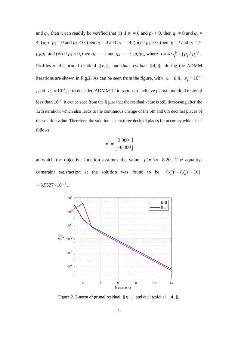

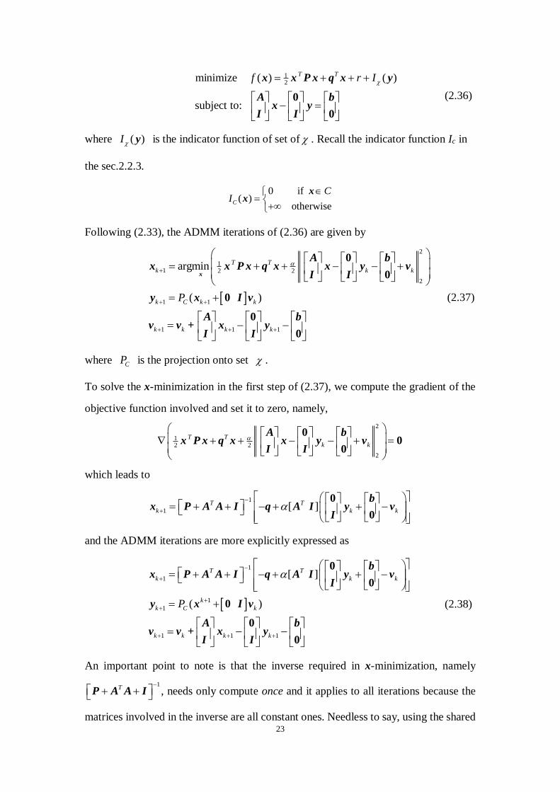


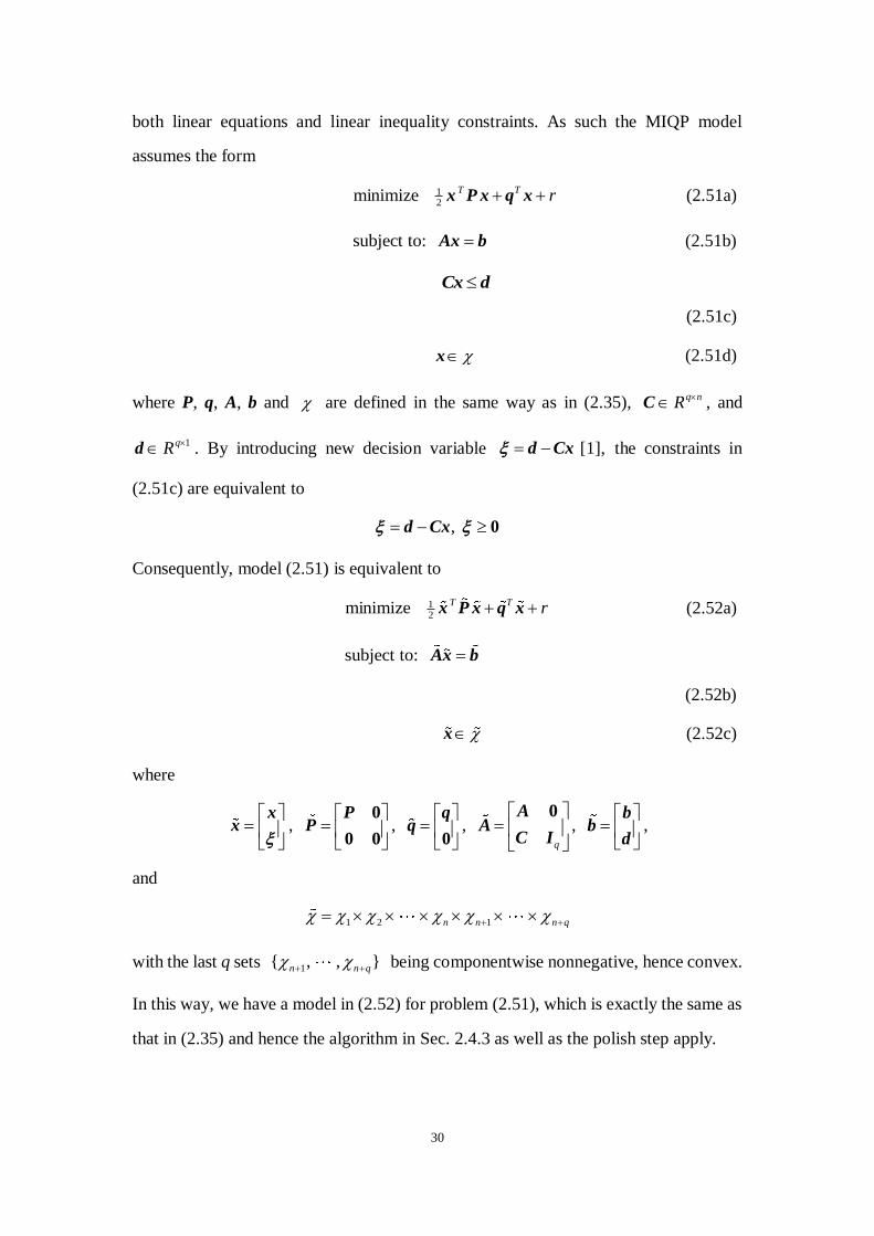


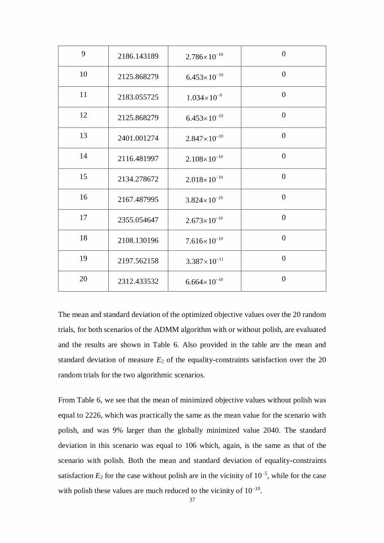

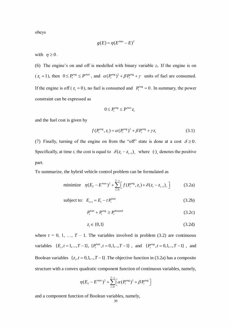

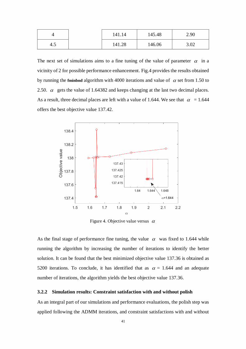
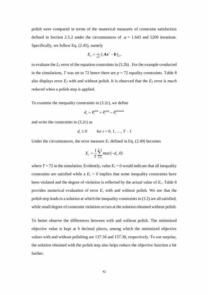


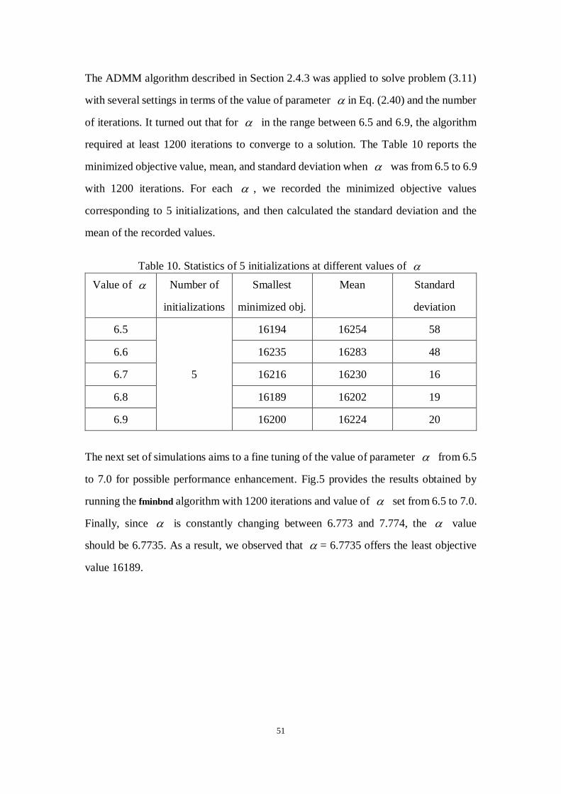


![Alternating Direction Method of Multipliers · CS 584 [Spring 2016] - Ho Practicalities and Tricks • ADMM usually obtains a relatively accurate solution in a handful of iterations,](https://img.dokumen.tips/doc/110x75/5b2b12f47f8b9af7088b4582/alternating-direction-method-of-multipliers-cs-584-spring-2016-ho-practicalities.jpg)