Computers and Chemical Engineering 26 (2002) 239–267

Algorithm architectures to support large-scale process systemsengineering applications involving combinatorics, uncertainty, and

risk management

Joseph F. Pekny *School of Chemical Engineering, Purdue Uni�ersity, West Lafayette, IN 47907-1283, USA

Received 18 April 2001; received in revised form 17 September 2001; accepted 17 September 2001

Abstract

Increased information intensity is greatly expanding the importance of model-based decision-making in a variety of areas. Thispaper reviews applications that involve large-scale combinatorics, data uncertainty, and game theoretic considerations anddescribes three related algorithm architectures that address these features. In particular, highly customized mathematicalprogramming architectures are discussed for time-based problems involving significant combinatorial character. These architec-tures are then embedded into a simulation-based optimization (SIMOPT) architecture to address both combinatorial characterand significant data uncertainty. Multiple SIMOPT objects are combined using a coordinating architecture to address gametheoretic issues. A key focus of the paper is a discussion of the algorithm engineering principles necessary to mitigate theNP-complete nature of practical problems. The life cycle issues of algorithm delivery, control, support, and extensibility areimportant to sustained use of advanced decision-making technology. An inductive development methodology provides a meansfor developing sophisticated algorithms that become increasingly powerful as they are subjected to new constraint combinations.Implicit generation of formulations is crucial to routine large-scale use of mathematical programming based architectures. © 2002Elsevier Science Ltd. All rights reserved.

Keywords: Risk management; Algorithm architectures; Combinatorics

www.elsevier.com/locate/compchemeng

1. Introduction

The global economy continues to undergo massivechanges. In contrast to the industrial revolution of theearly 20th century, which primarily effected society’sability to manipulate the physical world, these changesare being induced primarily by the explosive evolutionof information generation, management, and dissemi-nation. The World Wide Web and the Internet revolu-tion are a popular and well-documented example of theself-catalytic nature and speed of these changes. As theWeb and Internet technologies permeate society, theyare changing how people collect and use information.Indeed, businesses are beginning to learn to use theWeb and Internet in concert with other informationtechnology (e.g. personal computers, databases, etc.)

for rapid response to customer needs and opportunities.As such businesses are becoming acutely aware thatthey exist in a highly dynamic environment where speedand effectiveness of response is a matter of profitabilityand survival. This trend towards the speed at whichbusiness is conducted and important decisions have tobe made has significant implications for the need forProcess Systems Engineering (PSE). For purposes ofthis paper PSE is defined to be the coupling of engi-neering, physics, software, mathematics, and computerscience principles to address business and industrialapplications (see Grossmann and Westerberg (2000) fora more detailed discussion).

The Internet revolution to date has involved signifi-cant first order use of information. That is, this initialphase of the revolution made the same large body ofinformation available to anyone who could access theInternet. Of course the existence of and access to thislarge body of information generates value for society

* Tel.: +1-317-494-7901; fax: +1-317-494-0805.E-mail address: pekny@ecn.purdue.edu (J.F. Pekny).

0098-1354/02/$ - see front matter © 2002 Elsevier Science Ltd. All rights reserved.PII: S 0098 -1354 (01 )00744 -X

J.F. Pekny / Computers and Chemical Engineering 26 (2002) 239–267240

and prepares a foundation for next generation ad-vances (Magnusson, 1997; Phelps, 2002). A criticalnext generation advance, and one that the PSE com-munity is poised to contribute to, is the systematicprocessing of information into the knowledge ofwhich actions to undertake to achieve specific goals.In particular, the PSE discipline has developed for-malism for systematically translating information intodecisions in a goal-oriented fashion. In fact the speedof the economy in general and the speed at whichprofitability of a market attracts competition makesthe adoption of systematic means of transforming in-formation to knowledge essential. This follows be-cause the speed of the economy lessens the value of‘steady-state’ experience since companies now rarelyoperate in a static environment and companies needother means for generating a competitive advantagesince mere possession of information is a less signifi-cant advantage in an information rich environment.

In general terms, the PSE formalism for transform-ing information into knowledge involves (i) the analy-sis of a problem to understand its essential features,(ii) the construction of a model which captures theseessential features and provides a concise statement ofthe goal and constraints to achieving the goal, (iii) ameans of obtaining answers from the model, and (iv)interpreting the answers to understand the range over

which they are valid and how to implement them inpractice. A model is an expression of how variouspieces of information relate to one another and cantake on many different forms, for example a spread-sheet, a neural network, an expert system, a mathe-matical program, a regression equation, an x–y plot,etc. In virtually every successful application of PSEtechnology models undergo iterative refinement thatinvolves adapting the model to reflect continually im-proving understanding and an evolution of needs.Obtaining a solution to a model requires an al-gorithm for which the input is the specific data driv-ing the model and whose output is a solution to theproblem implied by the data. Insight is often gener-ated through repeated use of a model to understandhow output changes with input and this feedbackloop makes speed of solution an important consider-ation. Because of the theoretical difficulty in obtain-ing answers from models to most PSE problems (seePekny & Reklaitis, 1998), the discipline of algorithmengineering is critical to meeting the problem solvingchallenges.

Fig. 1 summarizes the motivation for this paper.As the progression of boxes shows, rapidly changingand abundant information induces a need to usemore sophisticated models to explain behavior. Inprocess and business applications these models oftenrequire making a number of discrete decisions. Givenreal world uncertainties there is a natural need tounderstand how decisions and risk depend on keyinformation. Many environments in which informa-tion is used involve multiple entities so that gametheoretic considerations are important to key deci-sions. The remainder of this paper discusses three re-lated algorithm architectures for addressing thebottom three boxes of Fig. 1. In particular, we reviewthe use of highly customized mathematical program-ming technology for problems involving large-scalecombinatorial optimization. This technology is in itsinfancy, but promises to systematically improve deci-sion-making in strategic, tactical, and real-time envi-ronments. The next section reviews examples wherelarge-scale combinatorial optimization is important.The following section describes a Mathematical Pro-gramming Based Architecture (MPA) for solvingmodels with a large combinatorial component. Subse-quent sections describe the Simulation-Based Opti-mization (SIMOPT) architecture for addressing riskmanagement and data uncertainty and an electronicProcess Investigation and Management Analysis(ePIMA) architecture for addressing game theoreticapplications. The role of algorithm engineering is alsodiscussed, especially as it applies to making the PSEmodeling formalism practical.

Fig. 1. Hierarchy of modeling issues motivated by abundant anddynamic information.

J.F. Pekny / Computers and Chemical Engineering 26 (2002) 239–267 241

Table 1Feature based scheduling problem classification

Description Industry sector

Pharmaceutical andMultiple small molecule products,specialty chemicalssimilar recipe structure,

campaigning/cleanout/setup,common production equipment

Long chain process, fixed batch sizes, Protein manufactureprocess vessel storage, dedicatedequipment

Identical recipe structure, large no. of Specialty blendingSKUs, single equipment processingfollowed by packaging, laborconstraints

Poly-olefins manufactureLimited shared storage, convergentprocess structure,campaigning/cleanout/setup, parallelequipment

Convergent recipe structure, shared Food and personal carestorage, renewable resourceconstraints, batch size limitations

Asymmetric parallel equipment, Large-scale printing andimplicit task generation, unlimited publishingstorage, multiple steps

of the combinatorial complexity of these applications isattributable to the management of time since manytypes of yes/no decisions can be thought of as recurringperiodically throughout the horizon of interest. Thisrecurrence of yes/no decision type can increase problemsize by one or more orders of magnitude depending onhow finely grained time must be managed. From apractical point of view the applications differ consider-ably in terms of data quality, organizational interest,end user skills, tool implementation issues, etc. How-ever, the purpose of this paper is to discuss the com-mon features of problems involving large-scalecombinatorics and algorithm architectures that may beengineered for their solution. A summary of each appli-cation domain and their relationship to each other is asfollows.

2.1. Process scheduling and planning

The problems in this domain are conveniently de-scribed using the resource-task-equipment framework(Pantelides, 1993). Resources can be considered renew-able or consumable according to whether they arereusable or are consumed upon use and must be replen-ished. Tasks can be thought of as actions that areapplied to resources. For example a reaction task caninput raw material resources at the beginning and thenemit product after a certain amount of time. Together aset of tasks defined to utilize a set of resources candefine an entire production network. Equipment is aspecial kind of renewable resource that is required inorder for a task to execute. In principle the resource-task description of a process is sufficient, but the redun-dancy of explicitly defining equipment provides a greatdeal more information to algorithms for solving processscheduling problems. In general the scheduling problemis to determine a time-based assignment of tasks toequipment so that no process constraints are violated.Typical constraints that must be satisfied are resourcebalances, inventory limitations (minimum and maxi-mums), unit allocation constraints, renewable resourcelimitations, and restrictions on how equipment may beused in time. The need to manage time greatly compli-cates the solution of process scheduling problems be-cause the interaction and tightness of these varioustypes of constraints can vary greatly, even in a singleproblem instance. For example the bottleneck piece ofequipment may change several times over the course ofthe problem horizon or the shortage of labor mayconstrain the schedule at particular times even thoughlabor may be abundant at other times. In fact, thevarious ways in which process scheduling constraintsmay interact over time gives rise to well-defined classesof problems. Table 1 summarizes the physical charac-teristics of a few of these classes of process schedulingproblems that are encountered in practice. The widely

2. Combinatorial nature of many process systemsapplications

Many PSE applications have a strong combinatorialcharacter. In principle, this combinatorial character canbe thought of as a series of yes/no questions that whenanswered in conjunction with specifying some relatedcontinuous variables values defines a solution to aproblem. This paper focuses on applications in theprocess management domain, including:� process scheduling and planning;� process design and retrofit;� model predictive decision-making;� warehouse management;� supply chain design and operation; and� product and research pipeline management.

The problems defined by these application domainsare difficult in the theoretical sense in that they arevirtually all NP-complete (see Garey & Johnson, 1979;Pekny & Reklaitis, 1998). In the intuitive sense they areintractable to solve using explicit enumeration al-gorithms for answering the yes/no questions since thereare typically hundreds to millions of yes/no decisions inproblems arising in practical applications. From thestandpoint of this paper, these application domains arerelated in the sense that they can utilize the sameunderlying technology for transforming information toknowledge. In particular the discussion of MPA,SIMOPT, and ePIMA is best motivated by understand-ing the key features of these related application areas.One key feature that unifies all the problems in theseapplication domains is the need to manage time. Much

J.F. Pekny / Computers and Chemical Engineering 26 (2002) 239–267242

different nature of these problem classes has criticalimplication on how to approach their solution as willbe discussed below. Goals in solving process schedulingproblems include minimizing cost, minimizing the num-ber of late orders, or maximizing process throughput(Applequist, Samikoglu, Pekny & Reklaitis, 1997;Reklaitis, Pekny & Joglekar, 1997).

2.2. Process design and retrofit

The process design and retrofit problem is a general-ization of the process scheduling problem in that allthe same decisions are required along with decisions asto when and how much equipment to add to a process.Process design and retrofit problems necessarily involvemuch longer time horizons than typical planningand scheduling problems because equipment purchaseand decommissioning plans are typically carried outover several years. This longer time scale of interestnecessarily introduces significant uncertainty, especiallyin the prediction of demands that will be placed onthe process. Thus process design and retrofit is typicallyconsidered a stochastic optimization problem thatseeks to optimize probabilistic performance. This per-formance usually involves maximizing expected netpresent value, minimizing expected cost, controllingrisk of capital loss, or maximizing an abstract meas-ure of process flexibility (Subrahmanyam, Bassett,Pekny & Reklaitis, 1995; Subrahmanyam, Pekny &Reklaitis, 1996; Epperly, Ierapetritou & Pistikopoulos,1997).

2.3. Model predicti�e decision-making

In practical applications decision problems are neversolved in isolation, rather decision problems arise peri-odically and must use as their starting point planspreviously in place as part of their solution. For exam-ple, many processes typically are scheduled once aweek or every few days. In determining a currentschedule, the execution in progress of a previous sched-ule, the available labor patterns, the arrival of rawmaterials, and the transportation schedule for productsare fixed by decisions made from having solved previ-ous scheduling problems. Thus decision problems arefrequently experienced as a related sequence in time.The solution of the current problem strongly dependson the previous members of the sequence and willaffect the solution of future problems. Thus in solvinga current problem, consideration must be given to thetypes of uncertain events that will perturb the ability tofollow a prescribed solution so that future problemscan be effectively solved. Model predictive scheduling,planning, or design problems have a close analogy tomodel predictive process control (see the summary ofQin & Badgwell, 2002).

2.4. Warehouse management

In abstract terms, the warehouse management prob-lem can be considered as a special kind of schedulingproblem. In particular, a warehouse consists of a num-ber of storage locations with capacities; there are anumber of resources that must be scheduled (e.g. labor-ers, fork trucks, etc.) to accomplish activities; and thereis a ‘raw’ material and ‘product’ delivery schedule. Ofcourse in the warehouse management problem, the‘raw’ materials are goods moved into the warehouseand the ‘product’ materials are goods moved out into atransportation network. Historically the warehousemanagement domain has been served by highly special-ized software. However, as upstream and downstreamproduction becomes more tightly integrated to ware-house management, the problems to be solved take oncharacteristics of both. The goal in warehouse manage-ment is to store material in such a way that the time toretrieve a set of material is minimized or that the costof warehouse operation is minimized. This goal is af-fected by how incoming material is assigned to storagelocations and how cleverly resources are used to ac-complish activities (Rohrer, 2000).

2.5. Supply chain design and operation

The supply chain operation problem extends thescheduling problem in the spatial dimension and con-siders the coordinated management of multiple facili-ties and the shipment of materials through anassociated transportation network. Because of theenormous size of supply chain management problems,significant detail is necessarily suppressed in their solu-tion. Similarly the supply chain design problem ad-dresses questions such as where a warehouse ormanufacturing facility should be located and to whichexisting site additional capacity should be added. Theincreased scope of supply chain management problemsand their long time horizons imply that they must besolved under significant uncertainty. Another dimen-sion involved in supply chain management are thegame theoretic aspects of cooperation, competition,and market factors. In particular many supply chainmanagement problems involve multiple entities, for ex-ample some of whom are suppliers, some of whom arecustomers, and some of whom are competitors. Thisadded dimension raises significant additional strategicquestions such as those concerning the pricing of prod-ucts, when to offer promotions, which type of incen-tives to offer customers to provide accurate demandforecasts, and how much inventory to hold to countermarket or competition shifts (see for example Tsay,1999). These strategic and game theoretic issues inter-act with the capabilities and scheduling of the facilitiesinvolved in the supply chain.

J.F. Pekny / Computers and Chemical Engineering 26 (2002) 239–267 243

2.6. Product and research pipeline management

The development of new products provides a com-petitive advantage for many companies and offers thepossibility of superior profitability when done consis-tently well. For example, the top-tier companies of thepharmaceutical industry possess billion-dollar drug de-velopment pipelines whose goal is to turn out block-buster products that provide substantial returns andunderwrite the cost of many candidates that fail tomake it to market. The product and research pipelinemanagement problem has much overlap both with sup-ply chain management and process scheduling prob-lems. In particular, correctly answering manymanagement questions depends on insight into howcompetitors will behave. This follows because the firstcompany to market with a particular product typeoften reaps the vast majority of market share andreturn relative to competitors that successively enter.Besides game theoretic issues, the many resources in apipeline must be coordinated to maximize the develop-ment throughput. Unlike manufacturing schedulingproblems, the scheduling of a product and researchpipeline involves a great deal of uncertainty as towhether all the tasks associated with the developmentof a particular product will be necessary. This is partic-ularly true of the pharmaceutical industry when candi-date drugs can be eliminated from consideration basedon safety and efficacy testing. The anticipated failure ofa significant fraction of all candidates leads to theconcept of ‘overbooking’ a pipeline whereby more tasksare scheduled for possible completion than could beachieved if all the candidates successfully survived. Thedifficulty in addressing practical problems is achievingthe proper amount of overbooking so that resources arefully utilized when attrition occurs but are not over-taxed (Honkomp, 1998).

2.7. Summary of features common to applications

As mentioned, all the above applications involve themanagement of activities over a time horizon. However,the discussion above also indicates several other com-monalities. In particular successful solution of any ofthese problems involves utilizing information that is notknown with great precision, for example demand fore-casts or which tasks will fail in a product and researchpipeline. This uncertainty implies that there will be riskin however the answers to the yes/no questions aremade. One challenge is to determine which pieces ofinformation are the most important to a good solution.Another challenge is to select an answer to a problemthat is the most effective over a wide range of possiblevalues of the most critical pieces of information. Thislast issue necessarily implies that risk management is animportant issue in many practical applications and that

steps must be taken because of uncertainty in underly-ing information that would be unnecessary if the infor-mation where completely known. Put succinctly, theabove applications involve (i) management of activitieson a timeline, (ii) significant combinatorial characterbecause of the large number of yes/no decisions impliedby practical applications, (iii) uncertain informationwhich can have a significant impact on the best answer,(iv) risk because the uncertainty might be realized in away that is detrimental, and (v) game theoretic aspectsbecause in many problems multiple entities interact.

3. Mathematical programming approach for processmanagement problems

A practical approach to process management prob-lems must be able to address each of the technicalissues summarized in the previous section as well as avariety of business process and human factors issues(see Bodington, 1995). The paper by Shobrys andWhite (2002) reviews typical and best practices foraddressing many process management problems usingtraditional technologies. This paper focuses on threerelated technologies that are general enough to addressthe applications described above, but which areamenable to the significant customization necessary forpractical use. The paper by Pekny and Reklaitis (1998)reviews various technologies and classifies them accord-ing to how they address the intrinsic computationaldifficulty of most process management problems. Asthey discuss virtually all process management applica-tions are NP-complete, the practical implication ofwhich is that there is an uncertainty principle that mustbe addressed in the development of any solution ap-proach. In particular, a given algorithm for a processmanagement problem cannot guarantee both the qual-ity of the answer and that the worst case performancewould not be unreasonable in terms of execution timeor computational resources. That is an algorithm mighttake an unreasonable amount of time to get a provablygood answer or might get an arbitrarily poor, or noanswer, in a predictable and reasonable amount oftime. Another useful way of interpreting the uncer-tainty principle is that any given algorithm that per-forms well on one process management problem willexhibit poor performance on some other process man-agement problem. This last statement sometimes seemsto contradict intuition, but can be understood by con-sidering the great variety of process management prob-lems and the fact that dominant features in someproblem will represent a combination of constraints onwhich previously known solution strategies are ill-suited. The importance of the uncertainty principle tousers, developers, and researchers of process manage-ment software cannot be overstated and indeed not

J.F. Pekny / Computers and Chemical Engineering 26 (2002) 239–267244

appreciating the practical implications of the uncer-tainty principle is a key cause of failure when processmanagement software does not work. The followingexample illustrates the implications of the uncertaintyprinciple on a simple problem.

3.1. Example: how an algorithm can fail when theproblem changes character

To understand the implications of the uncertaintyprinciple on a simple problem, consider a TravelingSalesman Problem (TSP) when all the cities to bevisited lie on a circle of a certain radius (circle-TSP). Anoptimal solution to the TSP involves specifying theorder in which cities are to be visited, starting andending at the home city, so that the travel distance isminimized. For the circle-TSP an algorithm guaranteedto find an optimal solution involves starting at thehome city, choosing the closest unvisited city as thenext city in the sequence, and repeating until all thecities have been traversed and then returning to thehome city. Of course this ‘greedy’ algorithm traces outa route in the order in which cities appear around thecircle (see Fig. 2). Now, when this same greedy al-gorithm is applied to a TSP whose cities appear at

random locations in a Euclidean plane its performanceis very poor because the greedy strategy does not takesteps to prevent having to traverse a long distance aftermost cities have been visited (see Fig. 3). The greedyalgorithm is an example of an algorithm whose execu-tion time is reasonable but whose solution quality canbe very bad. An alternative to the greedy algorithm isto exhaustively enumerate all possible solutions andchoose the one with the minimum travel distance. Suchan approach will guarantee arriving at a best possibleanswer, but the execution time will be unreasonable forall but the smallest problems. The papers by Miller andPekny (1991) and Pekny and Miller (1991) discuss thetradeoff between solution quality and performance inmore detail for versions of the TSP relevant to severalprocess scheduling applications. The TSP is one of themost well known problems in the combinatorial opti-mization literature and many highly engineered solutionapproaches have been developed that perform well onmany known classes of TSP instances-achieving opti-mal or near optimal solutions with reasonable effortand probability (Applegate, Bixby, Chvatal & Cook,1998). However, even for these highly engineered al-gorithms, instances can be constructed that cause themto produce poor answers or take unreasonable amountsof effort. When confronted with such a problematicinstance, existing TSP solution approaches can beadapted to provide better performance. Indeed thiskind of iterative challenge of TSP approaches has beena motivating factor in their improvement. Thus TSPalgorithms are an example of a research area that hasbenefited from iterative refinement motivated by thechallenge of problematic cases (for more informationsee the online bibliography by Moscato, 2002). Thisneed for iterative refinement is central to the engineer-ing of algorithms for any NP-complete problem.

3.1.1. Life cycle issues associated with the use ofalgorithms for practical problems

The key implication of the uncertainty principle isthat the development and use of process managementsolution algorithms is an engineering activity. The start-ing point of this engineering activity is that the objec-tives of the solution algorithm must be clearly stated.These objectives often include:1. guarantee of optimal solution,2. guarantee of feasible solution,3. guarantee of reasonable execution time,4. permits (requires) a high degree of user input in

obtaining an answer,5. high probability of obtaining a good answer in

reasonable time on a narrow and well-defined set ofproblem instances with limited user input,

6. easy to modify, adapt, and improve as new applica-tions or unsatisfactory performance is encountered,

7. low cost of development, and

Fig. 2. A ‘Greedy’ nearest neighbor algorithm works well on acircle-TSP.

Fig. 3. A ‘Greedy’ nearest neighbor algorithm works poorly on amore generalized TSP.

J.F. Pekny / Computers and Chemical Engineering 26 (2002) 239–267 245

8. provides an intuitive connection between solutionsand input data, that is explains why a given solutionwas obtained with the specified input data.

The theory of NP-completeness shows that insistenceon (1) or (2) as an objective precludes achieving (3) andvice versa. Experience shows that objectives (4) and (7)are highly compatible, but put much of the burden ofproblem solution on the user. Experience also showsthat objectives (5) and (6) seem complementary, butinconsistent with objective (7). Given the nature ofNP-completeness and the existence of the uncertaintyprinciple, objective (5) is a practical specification ofalgorithm engineering success and objective (6) speaksto how well an algorithm engineering approach sup-ports the life cycle encountered in applications. In thiscontext life cycle means the deli�ery of a solutiontechnology for use in practical applications, providingfor user control of the nature of answers to allow forincorporating considerations that are difficult to for-mally capture, support of a technology in the field whendeficiencies arise, and extension of a technology both tomake an individual application more sophisticated andfor use in a broader range of applications. An impor-tant part of user control is embodied in objective (8)whereby a solution can be rationalized and imple-mented with confidence because it is intuitively under-stood to be valid. This is especially critical forlarge-scale applications that involve enormous amountsof data, large solution spaces, and where an effectivesolution might represent a significant departure frompast practices. A key problem implied by (8) is theresolution of infeasible problems. In those applicationswhere tools are most useful the chance for specifying aninfeasible problem is greatest (e.g. too much demandfor the given capacity, insufficient labor to execute alltasks, etc.). In addition to being practically valuable,addressing objective (8) is an interesting research prob-lem given that there are sometimes many ways toresolve infeasibilities and discovering and presentingthese many options in a meaningful way is itself a verydifficult theoretical and computational problem (seeGreenberg, 1998). The paper by Shobrys and White(2002) suggests that objective (8) is crucial to the sus-tained acceptance of sophisticated modeling tools.Given the speed with which information is being gener-ated, the associated opportunities for improving effi-ciencies, and the need to rapidly reduce researchadvances to practice, all these life cycle considerations(delivery, control, support, and extension) are becomingan important part of PSE research. The remainder ofthis section discusses how mathematical programmingapproaches to process management problems promotesupport of life cycle issues and the remaining sectionsdiscuss their extension into risk management and gametheoretic applications.

3.1.2. Mathematical programming framework toaddress time-based problems

From an engineering standpoint, mathematical pro-gramming based approaches to process managementproblems offer a number of advantages. In particular amathematical programming based approach can delivermany combinations of the objectives (1)– (8), dependingon how it is implemented and used. For example,straightforward mathematical programming based ap-proaches will deliver objectives (1) and (2) at the ex-pense of ignoring (3). Experience also shows thatmathematical programming approaches can be used topursue objectives (5) and (6) at the expense of relaxingobjective (7), see for example Miller and Pekny (1991).Furthermore, mathematical programming approachescan easily support objective (4) and, as with otherapproaches, effective user input can make problemsmuch easier to solve. As our goal is the treatment ofapplication life cycle issues, the remainder of this sec-tion will discuss the use of mathematical programmingapproaches to achieve objectives (5) and (6) with theunderstanding that the same approaches can be used toachieve objective (1) and (2) or utilize objective (4),when necessary. With regard to addressing objective (8)mathematical programming methods have the advan-tage of a systematic framework for relating parametersand constraints, but the combinatorial complexity andambiguities inherent in explaining solution structureand resolving infeasibilities remains an important issueto be addressed by research (see Greenberg, 1998).

The starting point of a mathematical programmingbased approach is a formulation of a process manage-ment problem:

Maximize or Minimize f(x,y)

Subject to:

h(x,y)=0

g(x,y)�0

x�{0,1}m, y�Rn

The objective function of a process managementproblem is typically to minimize cost, maximize profit,minimize tardiness in the delivery of orders, etc. Theequality constraints typically implement material bal-ance or resource assignment constraints. The inequalityconstraints typically put restrictions on inventory andresource usage (e.g. labor). The binary variables (x)represent the discrete choices available when solving aprocess management problem, e.g. should an activity beexecuted on a given piece of equipment at a given time.The variables (y) represent the values of continuousquantities such as inventory levels or the amount ofmaterial purchased. There are two strategies for formu-lating process management problems. One strategy cre-ates time buckets and associates variables and

J.F. Pekny / Computers and Chemical Engineering 26 (2002) 239–267246

constraints with these buckets. Another strategy con-trols the sequencing of activities and only implicitlyrepresents time. Regardless of approach, the manage-ment of activities in time almost always makes the sizeof mathematical programming formulations for practi-cal problems quite foreboding.

3.1.3. Implication of the use of time bucketedformulations

The way that time is managed is critical to thesuccess of solving the process management problemsdiscussed above. We primarily use formulations wheretime is divided into buckets and constraints are thenwritten on variables that are associated with the timebuckets. For example, the material available in timebucket k is equal to the material available in timebucket k−1 plus the material that becomes available intime bucket k due to production minus the materialthat is consumed. Such material balance constraintsmust be written for every time bucket and material. Asanother example, consider that restrictions on the allo-cation of equipment yield constraints that have thefollowing form:

xmixing–activity–A,mixing–equipment,12 noon

+xmixing–activity–B,mixing–equipment,12 noon=1

This simple example shows that only one of mixingactivity A or B must be started on a piece of mixingequipment at 12 noon and shows how easily intuitionmay be expressed.

The work of Elkamel (1993), Kondili, Pantelides andSargent (1993), Pekny and Zentner (1994), and Zentner,Pekny, Reklaitis and Gupta (1994) discusses time buck-eted formulations in detail. Time bucketed formulationsoffer many advantages in applications and support lifecycle needs: (i) they are readily extensible to account foradditional problem physics, (ii) they are easy to under-stand since they are based on straightforward expres-sions of conservation principles and other problemphysics, and (iii) solution algorithm engineering is oftenfacilitated because reasoning can be localized due to thefact that variables and constraints only directly affectsmall regions of time. The chief drawback to timebucketed formulations is the size of formulation whenpractical problem detail is required. For example, con-sider that the need to provide 2 weeks worth of timelinemanagement with 1-h accuracy implies 336 time buck-ets and can easily translate to thousands or tens ofthousands of binary variables for practical applications.Furthermore, 1-h accuracy is insufficient for schedulingmany critical activities, e.g. the need to use labor for 10min at the start and end of an activity. In fact the timebuckets must be chosen to be as small as the smallesttime interval of interest. This type of reasoning quicklyleads to the conclusion that explicit formulation ofproblems using a time bucketing strategy leads to enor-

mous formulations and long solution times for mostpractical problems. This is because these large formula-tions take significant time to generate and an enormousamount of memory to store them, irrespective of thecost of actually obtaining a solution. Fortunately, mostof the constraints in time bucketed formulations ofpractical problems do not contribute meaningful infor-mation to problem solution because they hold trivially,e.g. zero equals zero. In practice, generation of thesetrivially satisfied constraints is not necessary. However,one does not realize which constraints matter until aftera solution has been obtained. Exploiting the large num-ber of trivially satisfied constraints and avoiding thegeneration of large explicit formulations is an engineer-ing necessity if a time bucketed mathematical program-ming formulation is to be delivered for use in practicalapplications.

3.1.4. Implicit techniques to a�oid large formulationsizes

The discussion in the preceding paragraph illustratesthe importance of considering all aspects of algorithmengineering when deciding how to approach solution ofan important class of practical problem. Whereas acommon means of using mathematical programmingapproaches is to generate the formulation and thensolve it, this explicit generation of a formulation is outof the question for many practical process managementproblems. Instead, we choose to pursue implicit genera-tion of only the nontrivially satisfied constraints andnonzero variables that are necessary for defining thesolution. Polyhedral cutting plane techniques also usethis strategy by utilizing separation algorithms to detectand iteratively enforce violated members of an expo-nentially large constraint family (Parker & Rardin,1988 and see the tutorial work of Trick, 2002). Theb-matching paper of Miller and Pekny (1995) illustratesthis implicit generation of both constraints and vari-ables and their approach is summarized in the followingexample.

3.2. Example: implicit formulation and solution of theb-matching problem

The b-matching problem with upper bounds may beformulated as an integer program on an undirectedgraph G= (V,E) with integer edge weights cij and in-teger edge variables xij as follows:

min �(i, j )�E

cij xij (1)

subject to:

�j�(i, j )�E

xij=bi, �i�V (2)

0�xij�dij (3)

J.F. Pekny / Computers and Chemical Engineering 26 (2002) 239–267 247

Fig. 4. Mathematical programming architecture for solving large-scale process management problems.

variables. Tree growth terminates when another vio-lated member of (6) is encountered and then the half-in-tegral variables can be made integral by modifying thevariables values of the half-integral cycles and in thetree according to a well-defined pattern (see Miller &Pekny, 1995). Thus growth of the tree identifies thenontrivial constraints of (6) which must be enforced.The nonzero variable values are identified by the net-work flow algorithm and tree growth. The highly cus-tomized implicit solution strategy summarized in thisexample has successfully solved problems with up to121 million integer variables in less than 10 min ofpersonal computer time (1 GHz, 128 Mb of RAM). Ofcourse most of these variables actually take on a valueof zero in the solution and only a few of the constraintsin (6) actually have to be enforced. See Miller andPekny (1995) for a complete description of the al-gorithm and a discussion of computational results.

Fig. 4 illustrates the basic concepts behind a mathe-matical programming architecture for solving processmanagement problems. The three main components are(i) implicit formulation— for example based on a timebucketed strategy (bottom box), (ii) an expert systemwhich controls the pivoting strategy used to solve thelinear programming relaxation of the formulation (topleft box), and (iii) an expert system that controls thebranching rules used during implicit enumeration (topright box). The b-matching example given above pro-vides a simple example of implicit formulation genera-tion and corresponding linear programming solution.Unlike the b-matching problem, process managementapplications produce linear programming relaxationsthat are arbitrarily integer infeasible and much lessstructured. In these cases the expert system choosespivots to provide for rapid linear programming solutionand to prevent the introduction of unnecessary infeasi-bilities. The work of Bunch (1997) provides an exampleof how pivot rules (i.e. an expert system for pivotingstrategy) can be used to avoid unnecessary infeasibili-ties. Avoiding such infeasibilities dramatically speedssolution since unnecessary implicit enumeration isavoided to remove these infeasibilities. For the b-matching problem described above the pivot rules de-scribed in Bunch (1997) reduce the computationalcomplexity of the guaranteed detection of violated con-straints from O(n4) to O(n), where n is the number ofnodes in the graph. The luxury of using a computation-ally cheaper algorithm to detect violated constraintsresults in order of magnitude speedup in problem solu-tion both because of faster convergence and fasteriterations. The advantage of the work of Bunch (1997)is that conventional linear programming solvers thatallow control of entering and exiting basic variablesmay be used to implement the technique.

Whereas implicit generation of mathematical pro-gramming formulations is crucial to the delivery of the

xij,dij�Z+ (4)

Relaxing the integrality constraints yields a LinearProgram (LP) that admits only integral and half-inte-gral solutions. The convex hull of the b-matching poly-tope as given by Padberg and Rao (1982) is useful fordeveloping a highly customized solution algorithm forthe b-matching problem. Let R�V with �R ��2, �(R)be the set of all edges with exactly one end in R, and Tbe a non-empty subset of �(R). A parity of R,T isdefined to be even or odd depending on the parity of:

b(R)+d(T)= �i�R

bi+ �e�T

de (5)

For this example �R,T is taken to mean all combina-tions of R and T with odd parity. Following Padbergand Rao (1982), the facet defining inequalities may bewritten as:

�(i, j )��(R)�T

xij+ �(i, j )�T

(dij−xij)�1, �R,T (6)

The implicit solution strategy of Miller and Pekny(1995) operates on the LP implied by (1)– (3), and (6) toobtain a provably optimal solution in a number of stepspolynomial in the cardinality of V. Note that (6) im-plies a number of constraints that scales exponentiallyin the cardinality of V. The basic idea behind theimplicit solution strategy is to use a network flowalgorithm, an implicit and highly customized linearprogramming solution technique, to solve (1)– (3). Theresulting solution will have integral and half-integralvalues. The half-integral values are eliminated by grow-ing a tree in graph G whose nodes represent eithermembers of V or individual constraints from (6). Cyclesmay be found during growth of the tree, which identifyother nontrivial constraints from (6) which are thendirectly enforced. The root of the tree is a violatedmember of (6) consisting of a cycle of half-integral

J.F. Pekny / Computers and Chemical Engineering 26 (2002) 239–267248

technology on practical applications, the architecture ofFig. 4 promotes extension of applications to encompassnew features. In particular, the solution logic is dis-tributed across the implicit generation of the formula-tion, the implicit enumeration expert system, and theexpert system for solving the LP. Both expert systemsare designed to operate on the formulation and there-fore are one level of abstraction removed from theproblem details. The expert system logic is coded toobtain solutions to the formulation and is not directlydesigned to deal with particular problem instances.Thus when the formulation is changed to encompassmore details or features, the basic expert system strate-gies for driving out infeasibilities are still valid. Ofcourse with due consideration to the uncertainty princi-ple described above, significant departures in problemfeatures from those that the expert systems have beenwell-designed to handle may cause a dramatic rise insolution time. This is especially true on large problemswhere even minor inefficiencies can result in unreason-able solution times due to the extremely large searchspaces implied by a large number of integer variables.When problematic cases occur, the abstraction of thesolution logic underlies a systematic approach for asso-ciating the cause in the solution logic to an undesirable

solution or unreasonable execution time. That is, thefeatures of the problem can be rationalized against theparticular sequence of pivots and the search tree path,which promotes physics based reasoning for failuresand expert system modifications that prevent encoun-tering them.

3.2.1. Mathematical programming architecture and lifecycle considerations

The paper by Pekny and Zentner (1994) discussed thebasic mathematical programming deli�ery architectureshown in Fig. 5 for process management applications.The basic components are (I) graphical user interface,(II) object oriented and natural language problem rep-resentation language, (III) mathematical programmingformulation, and (IV) solution algorithm (see alsoZentner, Elkamel, Pekny & Reklaitis (1998)). Obviouslya major benefit of the architecture of Fig. 5 is insulatingthe user from the details of the mathematical program-ming formulation and algorithm. With respect to lifecycle considerations and keeping in mind the need touse implicit formulations, the graphical user interfaceshown in Fig. 5 (I) is the means by which user controlis provided. In particular, the elementary and funda-mental nature of the variables in time bucketed mathe-

Fig. 5. Tool architecture promotes support of life cycle considerations.

J.F. Pekny / Computers and Chemical Engineering 26 (2002) 239–267 249

Fig. 6. Robust deployment through tool templatization.

matical programming formulations provides for manyclasses of user control. For example the simplest classof user control is to restrict a variable or group ofvariables to a particular value. With respect to manage-ment of time and equipment this class of user controlcan represent restricting (preventing) an activity to(from) a group of equipment or set of resources. Alter-natively, this class can restrict activities to a particulartime interval. Another class of user control possible isto direct the way in which the formulation is solved.For example, in a scheduling application a user canspecify that a particular demand be assigned resourcesbefore any other demand. This has the effect ofscheduling activities to satisfy the demand in a moreleft most position on the time line than demands thatare scheduled subsequently. An interrupt driven class ofcontrol is also possible whereby whenever an expertsystem considers manipulating a group of variables theuser can be prompted for direction as to how toproceed.

The architecture of Fig. 5 also promotes the supportof applications. Firstly, deciding where components ofFig. 5 execute in a client/server-computing environmentcan be made on the basis of the needs of the applica-tion. Second, the component represented in Fig. 5 (II)supports communication of problematic instances sincethe object oriented language description can be elec-tronically communicated to facilitate recreation of theproblem in a support environment. Perhaps most im-portantly from the standpoint of support, the architec-ture of Fig. 5 can be restricted to particular classes ofproblem instances where the probability of failure can

be kept low. Fig. 6 illustrates the concept of a ‘templa-tized’ tool whereby the graphical user interface andproblem description component are adapted to onlypermit the creation of instances that fall within a classfor which the tool has a high probability of solutionsuccess in terms of quality of answer and reasonableperformance, e.g. one of the problem types described inTable 1. In terms of product support there may only beone solution engine underneath all templatized tools,but the templates prevent users from applying the tooloutside the testing envelope. This eliminates many po-tential support problems, but still allows for extensionof the tool by relaxing the template restrictions. Interms of the circle-TSP example given above, templa-tization would amount to restricting the input to thegreedy algorithm to problems that are circle- or nearcircle-TSPs. By avoiding arbitrary Euclidean TSP in-stances a tool based on the greedy algorithm would notexhibit poor behavior. For any given algorithm archi-tecture, one qualitative measure of its versatility is thenumber of different problem types and the size ofproblem it can effectively address without additionalalgorithm engineering. Experience shows that thepromise of the algorithm abstraction of Fig. 4 is that byhaving the solution logic operate on the formulationinstead of the problem information directly that theversatility is enhanced.

3.2.2. A qualitati�e rating system for processmanagement applications

Given the uncertainty principle implied by NP-com-pleteness, a system for rating the effectiveness of solu-

J.F. Pekny / Computers and Chemical Engineering 26 (2002) 239–267250

tion algorithms provides a useful way of differentiatingdifferent approaches and implementations. Table 2 de-scribes a qualitative rating system for process manage-ment solution algorithms. The first column of Table 2shows the various classifications in the rating system,the second column provides a short description of theclassification, and the third column shows the re-sources/techniques that are likely to be required tomove an algorithm from one classification to a morecapable classification. The qualitative rating system ofTable 2 embodies the uncertainty principle, is sugges-tive of the different ways that solution algorithms canbe used and suggests that more robust behavior re-quires greater algorithm investment. One of the majoradvantages of mathematical programming approachesis that, with suitable investment, they can support theentire range of capability depicted in the first columnon a variety of problems through a formal and well-defined series of iterative refinements (also see the dis-cussion on problem generators in Kudva & Pekny,1993).

3.3. Example: detailed process scheduling applicationand discussion of mathematical programming approach

This example discusses a mathematical programmingapproach to a practical example from the modelingperspective through a model predictive application. Theexample is based on the Harvard Applichem case study(Flaherty, 1986) with the extensions described in Subra-manian (2001). The first part of the discussion summa-rizes the processing details and the second partdescribes the application.

3.3.1. Recipe networkThe Release-ease family of products moves through a

similar recipe, which consists of four tasks. The firsttask involves the all-important reaction where four rawmaterials A, B, C and D are added in a precise se-quence, along with miscellaneous substances includingwater (termed as ‘Other’) to yield a formulation ofRelease-ease particles. The Release-ease particlesformed move over a conveyer belt mesh in a cleaningtask where the liquid waste falls through. The filtrateparticles are further dried and packed in different sizes.The recipe is represented in Fig. 7.

The Gary, Indiana Applichem plant makes eightformulations in two grades, commercial and pharma-ceutical, and packs them in 79 packaging sizes selling atotal of 98 products.

3.3.2. Equipments/machinesThere are four categories of equipment used for the

production: reactors, conveyer belts, driers and packag-ing lines. The first task is executed in a reactor in batchmode. Three reactors with capacities 1000 and 8000 lbsalong with four more of an intermediate capacity of4000 lbs are available, totaling 10 in all. The processingtimes and Bills of Materials (BOM) depend on the typeof the formulation of Release-ease and on the batchsize. The reactors have to be washed out every time abatch is executed. Two identical conveyer belts filter theformed Release-ease. This is modeled as a batch taskwith processing times increasing proportionally withamount to be filtered. Three identical driers dry thefiltered Release-ease in batches. Eight packing linespack the eight formulations into 79 sizes making 98

Table 2Algorithm support classifications

Examples of resources required to improveAlgorithm capability Descriptionclassification

Algorithm is incapable of even small test problems with Extension of algorithm framework, fundamentalUnsupportedalgorithm modifications, intense R & D activityall constraint types

Algorithm is capable of demonstrating solutions butDemonstration Extension of algorithm framework to shape schedulessolutions are not implementable in practice, need according to user desires, interactive user interfacesculpting, and key constraints are not acceptably handled

Engineering Algorithm is capable of generating useful results, but Extension of algorithm framework to shape scheduleaccording to user desires, programmatic user interface,model solution is not sufficiently robust to use in practice

or some less important features are neglected which are interactive user interfaceof practical interest for routine use

‘Designed’ testing problems and generators to testRoutine Algorithm routinely generates useful schedules that areimplemented in practice through human interpretation, algorithm robustness, periodic minor coding fixes or

slight algorithm enhancementsroutine usage periodically results in the need for bug fixesor slight algorithm enhancements

Online model predictive Algorithm is extremely robust in generating schedules Generators to test algorithm robustness in anthat are faithful to shop-floor operations and can be used advancing time window fashion (SIMOPT based

testing—see later section)to predict shop-floor activity

J.F. Pekny / Computers and Chemical Engineering 26 (2002) 239–267 251

Fig. 7. Release-ease recipe.

Fig. 8. Material flow in the plant.

Stock Keeping Units (SKU) in all. It is assumed thatthe eighth packing line is dedicated to packaging com-mercial grade formulations, and hence packages fasterthan the other packing lines. There is no intermediatestorage prescribed after the cleaning task. It is assumedthat intermediate storage vessels are available after thereaction and drying tasks.

3.3.3. ProductsThe flow of materials (raw materials, intermediates

and final products) in the system is shown in Fig. 8. Theeight formulations are classified by grade (commercial(C) and pharmaceutical (P)) and particle mesh size (325,400, 600 and 800). Fig. 9 lists the final 98 products sold,differentiated by the packing type or size in which aformulation (such as C325) is packaged. P-xx refers toa packing type, and is assumed to correspond to aparticular size or shape.

3.3.4. Processing characteristics

3.3.4.1. Reaction task. The BOM for this task involvesinitial addition of B, C and Other together and uponcompletion of this reaction, addition of A and D. Theprocessing times are dependent on the grade and batchsize. The processing times, in minutes, are provided inTable 3. It is assumed that making 600 and 800 meshsize particles takes M times (see below) longer than 325

and 400. It is further assumed that making P gradetakes N times (see below) longer than C grade. ForM=N=1.2, processing times for all the grades areprovided in Table 3. The addition of A and D isassumed to take place after 10% of the overall process-ing time has elapsed.

3.3.4.2. Reaction wash-outs. The reactors have to becleaned after every batch execution. Washout times arelonger for larger reactors and after making P grade, dueto stricter environmental regulations. Washout timesare presented in Table 4.

3.3.4.3. Cleaning task. The cleaning times over theconveyer belt increase proportionally with the amountbeing filtered. The processing times are given in Table 5.

3.3.4.4. Drying task. Drying times are slightly longer forlarger batches. The drying times are listed in Table 6 asa function of output dried Release-ease quantities.

3.3.4.5. Packaging task. There are 79 distinct packingtypes based on size, and the packing times depend onthese types. The packing times are assumed to beindependent of the formulation being packaged. Table 7lists the packing times in hours, for all the 98 finalproducts along with the size they are sold in, inkilograms.

J.F. Pekny / Computers and Chemical Engineering 26 (2002) 239–267252

Table 3Processing times in minutes for the 8 grades

Fig. 9. Final products made by the Gary Applichem plant.

Table 5Cleaning times for conveyer belts

Table 6Drying times for release-ease formulations

3.3.4.6. Packing setups. Before a packing line executesthe packaging task, a setup time is incurred. This isrequired because there exists a need to arrange theappropriate packing type in the packing line. Thesesetups are reduced by 50% for the dedicated packingline 8. The setup data is provided in Table 8.

3.3.5. Material requirements and flowFor manufacture of 100 lbs of Release-ease, the raw

material requirements, as provided in the original Ap-

Table 4Wash-out times for reactors

J.F. Pekny / Computers and Chemical Engineering 26 (2002) 239–267 253

plichem case study (Flaherty, 1986), are presented inTable 9. The reactor batch is assumed to contain 10%Release-ease. This 10% figure represents the yield of theprocess. Therefore, 100 lbs of Release-ease would beproduced in a 1000 lbs batch with Other (1000–156.92)making up the total material amount to 1000. Becauseno intermediate storage is prescribed between the clean-

ing and drying tasks, they are modeled as a single task,which outputs the dried Release-ease particles inamounts of 100, 400 and 800 lbs (10% of the Reactorbatches). The rest of the material is discarded. Theseamounts of final product Release-ease are stored incontainers and packed into various sizes depending onthe demand.

Table 7Packing size in kg and packing times in hours for all final products

SKU ID Size Packing timeSKU ID Size Packing time

C400-P60 130C325-P11 1.520 0.1666666671.5150C400-P62C325-P12 0.16666666722

C325-P13 0.166666667 C400-P64 170 224C325-P14 2190C400-P660.16666666725

200C400-P67 20.33333333326C325-P15C400-P68 225C325-P16 228 0.333333333

30 0.333333333C325-P17 C400-P70 275 2.5C325-P18 C400-P7431 0.333333333 3375

32C325-P19 3475C400-P780.3333333330.33333333333 C600-P39C325-P20 55 0.5

C600-P41 60C325-P21 0.534 0.3333333330.33333333335 C600-P43 65 0.75C325-P22

C325-P23 0.333333333 C600-P45 70 0.75360.7575C600-P470.33333333337C325-P24

38 0.333333333C325-P25 C600-P49 0.758039C325-P26 0.7585C600-P510.333333333

0.33333333340 C600-P53C325-P27 90 0.75C600-P55 95C325-P28 0.7541 0.416666667

0.41666666742 C600-P57 100 1C325-P290.41666666743 C600-P65 180 2C325-P30

0.33333333330C800-P17C325-P31 0.416666667440.41666666745 C800-P27 40 0.333333333C325-P32

46 0.416666667C325-P33 C800-P37 50 0.4166666671120C800-P59C325-P34 0.41666666747

48C325-P35 1.50.416666667 140C800-P6149 0.416666667 C800-P63 160 1.5C325-P36

C325-P37 50 0.416666667 C800-P72 325 33C325-P57 100 4251 C800-P76

1.5 0.0166666671C325-P62 150 P325-P35 0.016666667C325-P67 200 2 P325-P5

P325-P7 10C325-P69 0.083333333250 23300 P325-P9 15 0.166666667C325-P71

P325-P11 20C325-P73 0.166666667350 3C325-P75 0.16666666725P325-P143400

30P325-P17 0.3333333333450C325-P773500 P400-P1 0.5 0.016666667C325-P79

30 0.333333333C400-P17 P400-P2 0.75 0.016666667C400-P27 0.0166666671P400-P30.33333333340

50 0.416666667C400-P37 P400-P4 0.016666667252.5C400-P38 0.01666666750.5 P400-P5

P400-P6C400-P40 7.557.5 0.0833333330.50.08333333312.5P400-P8C400-P42 0.7562.5

P400-P1067.5 17.5 0.166666667C400-P44 0.7572.5 0.75C400-P46 P600-P7 0.0833333331077.5C400-P48 0.75 0.16666666715P600-P9

P600-P11 20C400-P50 0.16666666782.5 0.75P800-P27 40C400-P52 0.33333333387.5 0.75

0.41666666750P800-P37C400-p54 0.7592.5C400-P56 0.7597.5

1C400-P58 110

J.F. Pekny / Computers and Chemical Engineering 26 (2002) 239–267254

Table 8Packing setup times for packing lines, X :{1…7}

D(t)=B+Gt+C sin(at)+S cos(at)+Noise

Here, B is the base demand, G is the growth or decay ofdemand, C is the coefficient for cyclic demand withperiodicity a, S is the coefficient for seasonal demandwith periodicity a, Noise is the normally distributednoise, �N(0,�), � is 5% of B.

Given such a demand profile over a specified horizon,the total demand quantity is apportioned amongst thesampled SKUs for every period in the horizon, based ona fixed ratio, thus generating the individual demands forevery SKU for every period.

3.3.7. ApplicationThe purpose of the application was to study scheduling

algorithm performance over a typical year of Gary plantoperation assuming that the plant was restricted tomanufacture a specified number of SKUs (5, 10, 20, 40,80) in any one 2 week period at various possible demandlevels. The Virtecs® scheduling system (version 4.021)with the Elise® MILP scheduling solver was used toconduct the study (Advanced Process Combinatorics,Inc., 2001). The plant is assumed to produce in amake-to-stock environment. Given the existence of themodel, the study could have investigated the effect ofadditional equipment, labor, technical improvements toreactor or other equipment performance, the marginalimpact of adding SKUs to the product mix, the effect offorecast noise on inventory levels, etc. To conduct thestudy, the timeline was divided into 52 1-week periodswith a reasonable initial inventory condition at the startof the timeline. A 2-week schedule was generated startingwith week number 1, the inventory at the end of the weekwas computed, and then the frame of interest wasadvanced 1 week and the process was repeated until 52overlapping 2-week schedules were generated for the 1year timeline. A typical 2-week Gantt Chart is shown inFig. 10 and a portion of this Gantt Chart is shown indetail in Fig. 11. The scheduling problem used to generateFig. 10 contained 178 tasks (reaction, etc.), 129 resources(products, intermediates), and 28 equipment items. TheGantt Chart in Fig. 10 contains 6710 scheduled activities(task instances=boxes on Gantt Chart). The problem inthis example is sufficiently large that a time bucketed (5min buckets) mathematical programming based ap-proach is only possible using an implicitly generatedformulation. Table 10 shows the execution time statisticsfor the Elise scheduling solver on a 400 MHz PentiumII with 256 Mb of memory after approximately 20 h ofalgorithm engineering effort. Table 11 shows the failurerate of the Elise scheduling solver on problem instancesat the beginning of the study prior to any algorithmengineering work. In this case failure is defined to be any1 year timeline in which the Elise solver required anunacceptably large amount of time to obtain a solutionon some scheduling problem along the timeline. For this

Table 9Raw materials consumed/100 lb release-ease produced

Raw material Amount (lbs)

A 20.7553.8B

C 53.6D 28.77Total 156.92

3.3.6. Product demandThere are two components to how demands are

estimated for use in the application below. The first is theproduct mix for which demands are specified, and thesecond pertains to the actual demand quantity specified.

3.3.6.1. Product mix. The 98 final products have beenclassified into three categories with high (0.6), medium(0.3) and low chance (0.1) of demands being specified.The number of products split between these categories is19, 46, and 33, respectively. If demands for ten productswere to be specified, six would be from the high category,three from medium and one from low. Even though 98products could be made and there is no restriction onhow many products can have demands specified, it isassumed that during normal plant operation only about20–40 products have demands specified in any one timeperiod. This assumption stems from usual industrialpractice of scheduling campaigns to smooth out noisylong-term demand signals, and rarely does a plant make100 different products in a short period of time. For theapplication described below, the number of SKUs forwhich demands would be generated is chosen and aparticular list of SKUs is obtained by sampling from thelist of 98 products.

3.3.6.2. Demand generation. Once the product mix isobtained, a total demand profile is created with the helpof a generic demand generator. The total demand overall the SKUs is generated using a sum of differentdemand signals. These signals are base demand, growthor decay with time, cyclic demands, seasonal demandsand random noise. The parameters that control each ofthe demand signals are set based on the desired charac-teristics in the total demand profile over time. Thedemand, D(t), for a period t is given as follows:

J.F. Pekny / Computers and Chemical Engineering 26 (2002) 239–267 255

study unacceptably large was defined to be more than 1h of execution time. As Table 11 shows, for schedulesinvolving certain numbers of SKUs the failure rate wasas high as 50% and as low as 0%. Upon completion ofthe algorithm work, the failure rate was 0% as mea-sured over 1300 2-week scheduling problems and theexecution time statistics of Table 10 show that thestandard deviation of execution times is small relativeto the mean indicating reliable performance. In order toconduct the algorithm engineering work several prob-lematic scheduling problems were studied to determinethe cause of the unreasonable execution time. In allcases the root cause of execution time failure wasdetermined to be due to numerical tolerances involvedin LP solution that had not failed on other problemtypes. The strategy used in applying the tolerances hadto be modified because of significant formulation de-generacy encountered in this application. The nature ofthese Applichem derived scheduling problems is suchthat very little enumeration is required so almost all thecomputational effort is spent on LP solution.

The scheduling literature contains several examplesof applications similar in size or larger that are solvedusing highly customized heuristics (Thomas & Shobrys,1988; Elkamel, Zentner, Pekny & Reklaitis, 1997).However, these heuristics are usually applicable only tothe specific problem for which they were designed.

Many of these heuristics lack the framework to express,let alone solve, such problem extensions as addinganother level of processing, parallel equipment, se-quence dependent changeover, shared or process vesselstorage, or combinations of these features. Some heuris-tic algorithms cannot address the addition of such acommonplace constraint as binding finite capacity stor-age. From an algorithm engineering point of view theseheuristic algorithms can be developed inexpensively rel-ative to customized mathematical programming basedapproaches. However, they lack extensibility since theirunderlying specialized representations cannot describefeatures beyond the problem for which they were de-signed. Lack of extensibility has significant practicalimplications. Processes typically evolve over time due tochanging prices of raw materials, new products, pres-sure from competitors, etc. An application that iswholly acceptable when installed, will certainly fall intodisuse if the underlying solution technology proves toobrittle to follow process evolution. Mathematical pro-gramming based approaches have the advantage thatthe solution methodology is built on an abstract prob-lem representation. The representation can often bechanged easily to accommodate process evolution(Zentner et al., 1994). Sometimes the solution method-ology will work as is, but NP-completeness guaranteesthat this cannot always be the case. This leads to the

Fig. 10. Two-week schedule for applichem case study.

J.F. Pekny / Computers and Chemical Engineering 26 (2002) 239–267256

Fig. 11. Grantt chart showing schedule detail.

notion of inductive development. A solution algorithmbased on an abstract representation will have beenengineered to solve a certain set of problems. When therepresentation is extended to address a new problemfeature, NP-completeness often requires additionalalgorithm engineering work. The inductive developmentprocess involves maintaining a set of problemsrepresentative of the neighborhood of success for thealgorithm, and the methodical extension of this set asproblematic cases are encountered. The key point of theinductive development process is that the improvedalgorithm will solve not only the new problematic cases,but also the entire set of representative problems.Mathematical programming based approaches cansupport the inductive development process through theuse of implicit formulation techniques. In fact theabove scheduling example was a problematic case thatwas brought into the solved set by mechanisticallyanalyzing the cause of failure and adapting the solutionapproach.

4. Simulation-based optimization architecture

As discussed above, process management problemsinvolve two issues that make their solution computa-tionally difficult:

Uncertain data: Much of the data used to driveprocess management is highly uncertain, for examplemarketing forecasts, the true cost of lost sales, andequipment failures. As such management strategiesmust be designed to work under a range of possibleconditions. Developing rational risk management poli-cies for a process involves exploring the tradeoffs be-tween the robustness of proposed plans to uncertainevents and the costs to achieve this robustness. Forexample, determining an appropriate inventory level ofa key intermediate involves trading off a carrying costagainst unexpected customer demand for any down-stream products or upstream production disturbances.The inventory carrying cost may be viewed as aninsurance premium for protecting against particulartypes of risks. Understanding the protection afforded

Table 10Final execution time statistics (in min) for 1300 2-week schedulingproblems

SKU Min. Max. Average S.D.

5.03829611.9396225.055 1.9833332.883333 57.7833310 30.91132 14.40239

20 3.883333 25.4 12.28382 3.9574225.99252140 0.9397764.516667 8.459.09891180 3.034012.95 14.73333

J.F. Pekny / Computers and Chemical Engineering 26 (2002) 239–267 257

Table 11Solver failure rate prior to any algorithm engineering effort

SKU Number of yearly runs made Num of yearly runs not solved Failure rate

75 0.51410 10 0 0

612 0.520540 1 0.2

80 7 0 0

by various levels of inventory helps keep costs to aminimum.

Combinatorial character: Even the most innocuousprocess management problems often have significantcombinatorial character due to the need to manageresources over time. This combinatorial character arisesfrom the need to address a series of yes/no questionswhose answers, for example, specify product sourcing,the use of different contract manufacturing options,transportation modes, raw material purchase alterna-tives, marketing strategies to promote demand, etc.

The need to simultaneously address both the combina-torial aspect and the impact of uncertain data is a keytechnical challenge in approaching process managementproblems. While there exist deterministic methods thataddress the combinatorial aspect (see the previous sec-tions) and simulation methods that use Monte Carlosampling to investigate the impact of uncertainty, mostexisting methodologies do not effectively address theinteraction of both to determine the best process manage-ment strategy. The approach described in this section isa computationally tractable approach for simultaneouslyconsidering combinatorial aspects and data uncertaintyfor industrial scale problems. The approach builds onwell known simulation methods and deterministic meth-ods for large-scale problems, such as those described inthe previous section.

The SIMOPT architecture, as shown in Fig. 12, usesa customized mixed integer linear programming solver tooptimize process behavior in conjunction with a discreteevent simulator to investigate the effect of uncertainty onthe plans output from the optimizer. The optimizersolution provides the initial input to the simulation andthe simulation returns control to the optimizer wheneveran uncertain event causes infeasibility that necessitates anew plan. Thus the iteration between the simulation andoptimization continues until a timeline is traced out fora sufficiently long horizon of interest. The informationgenerated along this timeline represents an example ofhow the future could unfold. As this process is repeatedalong different timelines for different simulation sam-plings (see Fig. 13), the evolution of behavior can bevisualized in many possible realities. From a risk man-agement perspective, the goal is to optimize the here-and-now decisions so that they perform well across a large

fraction of the possible timelines. Of course the here-and-now optimization problem embodies the set of choicesfaced by planners and the SIMOPT approach allowsthem to gauge whether their decisions involve an accept-able amount of risk. One objective that can be used inthis stochastic optimization is the lowest cost to achievea certain level of risk. Risk is specified in terms of limitingthe probability of certain goals not being achieved or

Fig. 12. Architecture of simulation-based optimization algorithm forcombinatorial optimization problems under parametric uncertaintyand for risk analysis.

Fig. 13. Timelines traced by simulation-based optimization architec-ture.

J.F. Pekny / Computers and Chemical Engineering 26 (2002) 239–267258

Fig. 14. Seven project example.

where the goal is to maximize the rewards from success-fully completing tasks over a 19 week horizon. Thisexample is closely related to the scheduling example inthe previous section in that the tasks in the pipeline mustbe scheduled so as not to utilize more resources than aredynamically available. As such a time bucketed schedul-ing formulation is used by the optimizer. In the pipelinethere are the seven projects shown in Fig. 14 whoseactivity details are given in Table 12 and expected rewarddata are given in Table 13. Each activity has a duration,requirements for two different resources, and a probabil-ity of success. Each of these parameters is represented bya probability distribution as shown in Table 12. Theduration and resource requirements are represented bya custom distribution that specifies a value and itsassociated probabilities. The activity success probabili-ties are represented by a triangular distribution. Inpractice the custom distributions could be specifiedsimply as high, medium, and low values since estimatingmore detailed distributions is too tedious for manypurposes. For this example there are 16 units of resourceR1 and 8 units of resource R2 available. The distribu-tions associated with each parameter are used by thesimulation component to trace out timelines of possiblepipeline behavior. The data given in Tables 12 and 13 arealso used by the optimization component to schedulepipeline activities. An example schedule is given in Fig.15 after the simulation component has sampled the taskduration and resource requirement distributions. Notethat the schedule shown in Fig. 15 only includes a subsetof the projects because resource requirements limit thenumber of activities that may be simultaneously exe-cuted. In generating the schedule of Fig. 15, the optimiza-tion component was executed three times, to develop aninitial schedule, to develop a schedule after activity I2(project 1) failed, and after activity I6 (project 3) failed.Note that Fig. 15 only illustrates the initial portion of apossible timeline and that the simulation could beextended until all projects either fail or are executed. Amore realistic simulation could also introduce newprojects at later times. Each time the simulation isexecuted a new timeline is generated corresponding toone possible outcome of the pipeline. After many execu-tions, a distribution of pipeline behavior is obtained. Fig.16 shows the distribution of pipeline performance after20 000 timelines are generated. Two distinct classes ofperformance are illustrated in Fig. 16. One class ofperformance is associated with timelines that experiencean average reward of about $8000. Another class ofperformance is associated with timelines that experiencean average reward of about $34 000. The more valuableclass of performance is associated with the success of ablockbuster project. A close inspection of Fig. 16 showsthat several timelines also exhibit behavior between thetwo dominant classes. Thus Fig. 16 illustrates that evena relatively small problem involving only a few projectsexhibits complex behavior that arises because of uncer-

limiting the probability that a process will not achieve acertain level of performance.

A key challenge of the basic scheme shown in Fig. 12is maximizing the rate at which meaningful samples canbe collected so that the overall procedure completes ina reasonable time, even for realistic problem sizes. Thischallenge can be met with two basic strategies: (1)maximizing the speed at which the optimizer executes (asin the previous section), and (2) biasing the parametersampling procedure so that the simulation focuses on‘critical events’ and avoids a large number of simulationswhich are not particularly insightful. Strategy number (2)essentially requires using a procedure for identifyingwhich uncertain events are problematic for a given planand then biasing the sampling to explore them. Acorrection must be applied to accurately estimate thesystem behavior probabilities from the biased sampling(see Kalagnanam & Diwekar (1997), Diwekar &Kalagnanam (1997)).

A related challenge of the SIMOPT approach isdetermining when control should pass from the simulatorto the optimizer. In particular, the response to anuncertain event can be to make local changes at a giventime point in the simulator or to invoke the optimizer toeffect more global changes. Obviously the more fre-quently the optimizer is invoked the slower the overallprocedure, but the better the quality of the reaction.Practically the key to meeting this challenge is to deter-mine an optimization frequency whereby if the optimizeris invoked more frequently the overall result does notchange by an appreciable measure. The paper by Subra-manian, Pekny and Reklaitis (2001) describes the issuesinvolved with selecting reasonable trigger events andtheir associated computational expense.

4.1. Example: simulation-based optimization applied toan R & D pipeline

As an example of the SIMOPT approach considermanagement of a research and development pipeline

J.F. Pekny / Computers and Chemical Engineering 26 (2002) 239–267 259

Table 12Data for seven-project example

R1 (units), customActivity R2 (units), custom Probability success triangularDuration (weeks), customdistribution distribution distribution distribution

ValueValue Probability Value Probability Min. Most likely Max.Probability

I1 41 0.29 2 0.28 0.74 0.80 0.860.2955 0.44 3 0.440.37526 0.21 4 0.283 0.1907 0.060.1104

5 0.0304 0.06 1 0.220.10 0.7I2 0.75 0.825 0.21 2 0.563 0.186 0.46 3 0.160.4447 0.21 4 0.065 0.188 0.060.106

10 0.06 2 0.29P1 0.83 0.85 0.90.3211 0.12 3 0.440.404125 0.55 4 0.210.1813 0.21 5 0.060.10614 0.063 0.05 1 0.230.335 0.7I3 0.8 0.8514 0.20 2 0.522 0.4155 0.45 3 0.200.16636 0.25 4 0.054 0.0847 0.054 0.23 1 0.23I4 0.553 0.6 0.650.1235 0.52 2 0.550.20346 0.20 3 0.165 0.3357 0.05 4 0.060.2286

7 0.11110 0.23 2 0.230.32 0.754 0.8 0.85P211 0.55 3 0.535 0.4412 0.16 4 0.160.166

7 0.08 13 0.06 5 0.082 0.23 1 0.230.26 0.7I5 0.8 0.8523 0.55 2 0.533 0.544 0.15 3 0.170.1445 0.07 4 0.075 0.064 0.23 1 0.2250.10 0.73 0.75 0.8I65 0.53 2 0.5654 0.206 0.17 3 0.1550.3657 0.07 4 0.0556 0.28

0.06712 0.225 2 0.225P3 0.854 0.9 0.950.3213 0.555 3 0.5550.40514 0.160 4 0.1606 0.1815 0.060 5 0.0600.107

3 0.23 2 0.23I7 0.853 0.9 0.950.3354 0.55 3 0.550.41545 0.155 4 0.150.1656 0.07 5 0.070.08565 0.23 1 0.23I8 0.551 0.6 0.650.3356 0.57 2 0.570.41527 0.15 3 0.153 0.1658 0.05 4 0.050.08544 0.23 1 0.22I9 0.651 0.7 0.750.325 0.57 2 0.560.4026 0.153 3 0.160.187 0.05 4 0.060.1049 0.23 2 0.23P4 0.754 0.8 0.850.07

10 0.53 3 0.530.17511 0.176 4 0.170.5212 0.07 5 0.070.177

8 0.07

J.F. Pekny / Computers and Chemical Engineering 26 (2002) 239–267260

Table 12 (Continued)

R2 (units), customR1 (units), customDuration (weeks), custom Probability success triangularActivitydistributiondistribution distribution distribution

Most likelyValue Probability Value Probability Value Probability Min. Max.

0.7 0.85I10 3 0.850.33 4 0.23 3 0.230.544 0.41 5 0.53 40.1750.1760.205

0.066 0.0660.0772I11 6 0.230.297 3 0.23 0.38 0.38 0.483 0.456 7 0.54 4 0.534 0.197 8 0.17 5 0.17

0.0760.0690.0550.380.380.231 0.480.2350.321I12

2 0.42 6 0.53 2 0.533 0.18 7 0.17 3 0.17

0.0740.0780.0840.750.70.232 0.80.23110.3253P5

4 0.375 12 0.53 3 0.535 0.150 13 0.17 4 0.176 0.100 14 0.07 5 0.077 0.050

0.70.23 0.80.75I13 3 0.305 4 0.23 30.440 5 0.53 44 0.53

5 0.200 6 0.17 5 0.176 0.055 7 0.07 6 0.07

0.2330.236 0.40.323I14 0.45 0.50.5340.5370.424

5 0.18 8 0.17 5 0.176 0.08 9 0.07 6 0.07

0.70.650.60.223P6 0.20130.08834 0.200 14 0.57 4 0.545 0.380 15 0.23 5 0.176 0.280 6 0.07

0.05270.70.2230.22 0.8540.3253I15 0.85

0.5440.5450.42545 0.175 6 0.17 5 0.176 0.075 7 0.07 6 0.071 0.283 6 0.22I16 5 0.450.22 0.550.5

0.5460.5470.43320.1770.1780.2843

9 0.07 8 0.070.3 0.35I17 2 0.29 6 0.40.22 2 0.22

0.5430.5470.4430.1740.1780.214

5 0.06 9 0.07 5 0.070.55P7 3 0.29 13 0.20 3 0.22 0.45 0.5

4 0.44 14 0.57 4 0.545 0.21 15 0.23 5 0.17

60.066 0.07

tainty and resource contention. SIMOPT type ap-proaches provide insight into this range of behavior,but there are several issues that must be addressed inpractical applications. In particular, the nature of howrewards are computed has a significant effect on results.This example assumes that 10% of the reward is re-ceived after completion of the initial steps of the projectand the remaining 90% of the reward is received aftercompletion of the final step. Another strategy is toassume that all rewards are received only after the

completion of the final step. Which assumptions areused for the rewards depends on the purposes of thestudy. If proper care is exercised in setting up theproject parameters, this example shows that SIMOPTcan be used to develop intuition about particular eventsthat can occur (Fig. 15) and the classes of behavior thatmay be encountered in operating the pipeline (Fig. 16).The combined use of optimization and simulation pro-vides a great deal of realistic insight because the sched-ules that are generated satisfy all the resource constra-

J.F. Pekny / Computers and Chemical Engineering 26 (2002) 239–267 261

Table 13Project reward data

Project Reward $

P1 30 000P2 20 000P3 15 000P4 40 000P5 50 000P6 40 000P7 60 000

Fig. 16. Distribution of rewards for the seven-project example after20 000 timelines are generated.

ints and the distribution information can be used tomanage risk. More details about SIMOPT and thisexample may be found in Subramanian, Pekny andReklaitis (2001).

5. ePIMA: architecture for investigating game theoreticapplications

In addition to combinatorial and uncertainty consider-ations, many practical problems involve multiple entitiesthat must cooperate or compete in some environment.These types of game theoretic issues are most often foundat the supply chain management level, but are importantin any process management problem where significantbehavior can only be modified indirectly. Traditionally,game theoretic issues are only addressed with relativelycoarse approaches that neglect details to more fully focuson how cooperation or competition takes place. How-ever, to accurately address many applications requiresconnecting game theoretic issues to process details. Forexample, effectively setting the proper pricing or timingof a consumer product promotion can depend on man-ufacturing operations (e.g. inventory levels, changeovercosts, waste, etc.) and a competitor’s manufacturing

operations. Ideally, a promotion must be timed wheninventory levels and manufacturing capacity can accom-modate additional demand and puts a competitor at adisadvantage. Available to Promise (ATP) dates forpotential product delivery are another example of whereconnecting game theoretic issues to process detail offerssignificant opportunity. The most effective ATP datesmust take into account inventory levels, available processcapacity, the importance of the customer, and currentprocess operations. If the wrong ATP date is given thiscan result in a lost product sale or requiring extra costto satisfy the order. Effective ATP dates can involvedifferent product pricing levels or sharing demand fore-casts between suppliers and customers so that deliverydates can be cooperatively determined. Examples ofother process management questions where both detailand game theoretic issues are important include:

Fig. 15. A possible schedule for the seven-project example.

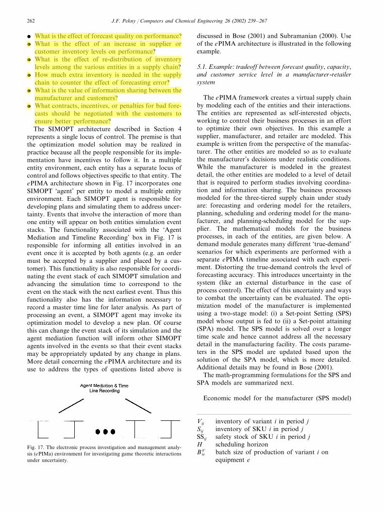
J.F. Pekny / Computers and Chemical Engineering 26 (2002) 239–267262

� What is the effect of forecast quality on performance?� What is the effect of an increase in supplier or

customer inventory levels on performance?� What is the effect of re-distribution of inventory

levels among the various entities in a supply chain?� How much extra inventory is needed in the supply

chain to counter the effect of forecasting error?� What is the value of information sharing between the

manufacturer and customers?� What contracts, incentives, or penalties for bad fore-

casts should be negotiated with the customers toensure better performance?The SIMOPT architecture described in Section 4

represents a single locus of control. The premise is thatthe optimization model solution may be realized inpractice because all the people responsible for its imple-mentation have incentives to follow it. In a multipleentity environment, each entity has a separate locus ofcontrol and follows objectives specific to that entity. TheePIMA architecture shown in Fig. 17 incorporates oneSIMOPT ‘agent’ per entity to model a multiple entityenvironment. Each SIMOPT agent is responsible fordeveloping plans and simulating them to address uncer-tainty. Events that involve the interaction of more thanone entity will appear on both entities simulation eventstacks. The functionality associated with the ‘AgentMediation and Timeline Recording’ box in Fig. 17 isresponsible for informing all entities involved in anevent once it is accepted by both agents (e.g. an ordermust be accepted by a supplier and placed by a cus-tomer). This functionality is also responsible for coordi-nating the event stack of each SIMOPT simulation andadvancing the simulation time to correspond to theevent on the stack with the next earliest event. Thus thisfunctionality also has the information necessary torecord a master time line for later analysis. As part ofprocessing an event, a SIMOPT agent may invoke itsoptimization model to develop a new plan. Of coursethis can change the event stack of its simulation and theagent mediation function will inform other SIMOPTagents involved in the events so that their event stacksmay be appropriately updated by any change in plans.More detail concerning the ePIMA architecture and itsuse to address the types of questions listed above is

discussed in Bose (2001) and Subramanian (2000). Useof the ePIMA architecture is illustrated in the followingexample.

5.1. Example: tradeoff between forecast quality, capacity,and customer ser�ice le�el in a manufacturer-retailersystem

The ePIMA framework creates a virtual supply chainby modeling each of the entities and their interactions.The entities are represented as self-interested objects,working to control their business processes in an effortto optimize their own objectives. In this example asupplier, manufacturer, and retailer are modeled. Thisexample is written from the perspective of the manufac-turer. The other entities are modeled so as to evaluatethe manufacturer’s decisions under realistic conditions.While the manufacturer is modeled in the greatestdetail, the other entities are modeled to a level of detailthat is required to perform studies involving coordina-tion and information sharing. The business processesmodeled for the three-tiered supply chain under studyare: forecasting and ordering model for the retailers,planning, scheduling and ordering model for the manu-facturer, and planning-scheduling model for the sup-plier. The mathematical models for the businessprocesses, in each of the entities, are given below. Ademand module generates many different ‘true-demand’scenarios for which experiments are performed with aseparate ePIMA timeline associated with each experi-ment. Distorting the true-demand controls the level offorecasting accuracy. This introduces uncertainty in thesystem (like an external disturbance in the case ofprocess control). The effect of this uncertainty and waysto combat the uncertainty can be evaluated. The opti-mization model of the manufacturer is implementedusing a two-stage model: (i) a Set-point Setting (SPS)model whose output is fed to (ii) a Set-point attaining(SPA) model. The SPS model is solved over a longertime scale and hence cannot address all the necessarydetail in the manufacturing facility. The costs parame-ters in the SPS model are updated based upon thesolution of the SPA model, which is more detailed.Additional details may be found in Bose (2001).

The math-programming formulations for the SPS andSPA models are summarized next.

Economic model for the manufacturer (SPS model)

Vij inventory of variant i in period jinventory of SKU i in period jSij

safety stock of SKU i in period jSSij

scheduling horizonHbatch size of production of variant i onBie

V

equipment e

Fig. 17. The electronic process investigation and management analy-sis (ePIMa) environment for investigating game theoretic interactionsunder uncertainty.

J.F. Pekny / Computers and Chemical Engineering 26 (2002) 239–267 263

batch size of production of SKU i on equip-BieS

ment eprocess time for batch of variant i in period jt ije

V

on equipment eprocess time for batch of SKU i in period jt ije

S

on equipment enije

V number of batches of variant i produced inperiod j on equipment e

number of batches of SKU i produced in pe-nijeS

riod j on equipment enumber of variantsNV

number of SKUsNS

set of equipments for producing variantsEV

set of equipments for producing SKUsES

MV matrix representing the bill of materials forstage I (purification of variants)

matrix representing the bill of materials forMS

stage II (packing of SKUs)c cost of raw materialsPV production costs for stage I (purification of

variants)production costs for stage II (packing ofPS

SKUs)PM price mark-up for SKUshRM holding cost of raw materials per unit weight

per periodholding cost of variants per unit weight perh�

periodhs holding cost of SKUs per unit weight per

periodps penalty cost of missed demands for SKUsSij

+ dummy positive variable representing overageof SKU i in period j

dummy positive variable representing under-Sij−

age of SKU i in period jsafety stock of SKU i in period jSSij

demand of SKU i in period jDij

t jeD downtimes and changeover-time on equipment

e in period jtT total time available in a period

The SPS model seeks to maximize profit that isdefined as revenue minus costs. The costs have threecomponents, which are holding costs, penalty costs andproduction costs. The objective function is given below.For succinct matrix representation, the index i pertain-ing to the resource (SKU or variant) is dropped.Max (profit)= �

H

j=1

[(revenue)j− (costs)j ] (7)

where,

((revenue)j

= (c MVMS+PVMs+PS)(Dj−Sj−)(1+PM) (8)

(costs)j=hsSj++hRMRj+psSj

−+PV �EV

e=1

njeV+PS �

ES

e=1

njeS

(9)

The modeling of penalty and holding costs becomeseasy by introducing two dummy independent variables,representing the underage (Sij

−) and overage (Sij+) of

inventory. The actual inventory in any week for a SKUis given by the following equation.

Sij=Sij+−Sij

− (10)

The variables Sij+ and Sij

− cannot take negative valuesand both Sij

+ and Sij− cannot be positive at the same

time.The above objective function is subject to various

constraints. The following sets of equations are themass balance constraints, which link the inventory fromone period to the next.

Sij=Si( j−1)+ �e�E S

[nijeS Bie

S]−Dij �i� [1,NS ], �j� [1,H ]

(11)

Vij=Vi( j−1)+ �e�E V

[nijeV Bie

V]− �e�E S

{M ieS[nije

S BieS]}

�i� [1,NS ], �j� [1,H ] (12)

The constraint determines the raw material inventorythat should be available at the beginning of eachperiod.

Rj� �e�E V

[MV(njeVBe

V)] �j� [1,H ] (13)

The next two equations enforce the condition that thetotal production time, downtime and changeover-timesdo not exceed the total available time in a period.

�NS

i=1

[t ijeS n ije

S ]+ t jeD� tT �j� [1,H ], �e�ES (14)

�NV

i=1

[t ijeV nije

V ]+ t jeD� tT �j� [1,H ], �e�EV (15)

The lower and upper bounds for the independent vari-ables are given below.

0�Sij+�Smax

+ �i� [1,NS ], �j� [1,H ] (16)

0�Sij−�Smax

− �i� [1,NS ], �j� [1,H ] (17)

0�Vij�Vmax �i� [1,NV ], �j� [1,H ] (18)

0�Rij�Rmax �i� [1,NV ], �j� [1,H ] (19)

yijeS �{0,1} �i� [1,NS ], �j� [1,H ], �e�ES (20)

yijeV �{0,1} �i� [1,NV ], �j� [1,H ], �e�EV (21)

5.1.1. Scheduling model for manufacturer ( first SPAmodel)

The manufacturer uses the SPA (scheduling) modelto attain the target inventory levels set by the SPS

J.F. Pekny / Computers and Chemical Engineering 26 (2002) 239–267264

model. In order to avoid being myopic the manufac-turer plans for several periods ahead in advance in theSPS model. However, the SPA model is only invokedfor the first period in order to obtain a detailed sched-ule for that period. The SPA model is defined andsolved with the VirtECS® scheduler (Advanced ProcessCombinatorics, Inc., 2001). Before the SPA model isformulated, the solution of the SPS model is processedto compute the demands for the scheduling problem.Based on the solution of the SPA model, the productcosts in the SPS model are updated and the SPS modelis resolved. This updating is done to reflect the actualvalues of the products cost parameters.

5.1.2. Ordering model for the manufacturer (second SPAmodel)

The model is based upon dynamic lot-sizing wheredemands are known but vary over time. This singleitem model is solved for each SKU.

Let, H is the planning horizon (the number of peri-ods for which demands are known in advance), Dj isthe forecast demand in period j, j= [1, H ], cj is the unitpurchase cost in period j, j= [1, H ], K is the fixed(set-up) cost incurred when an order is placed in periodj, j= [1, H ], h is the holding cost incurred to carry anunit of inventory from period j to ( j+1), j= [1, H ], Ij

is the amount of product inventory at the start of aperiod t (before ordering), j= [1, H ], and Qj is the orderquantity for period t (to be determined), j= [1, H ].

The formulation seeks to determine Qj in order tominimize the total cost (holding cost plus fixed-orderingcost) while satisfying all demands (no back orders) (seeBose, 2001 for details). It is assumed that the purchasecost of items is constant over time. Thus cj=c for allj= [1, H ].

The objective function tries to minimize the sum ofholding costs and ordering costs. Since it is assumedthat the ordering models will order so as to fulfill alldemands for raw materials, the penalty cost for missingany demand is not considered in the model. The objec-tive function is given as follows:

Min �H

j=1

[hIj ]+ �H

j=1

[K�(Qj)] (22)

Here the delta function (�) takes the value 1 if Qj ispositive, 0 otherwise. The above objective function issubject to several constraints. The first constraint is amaterial balance constraint.

Ij=Ij−1+Qj−Dj �j� [1,H ] (23)The upper and lower bounds for the variables arespecified in the problem. They are given as:

0�Ij�Imax �j� [1,H ] (24)

0�Qj�Qmax �j� [1,H ] (25)

Let the lead-time between the manufacturer and the

retailers is L periods. Thus, quantity, Qj ordered inperiod j will be received in period j+L. Eq. (23)changes to:

Ij+L=Ij+L−1+Qj−Dj+L �j� [1,H ] (26)

We provide below a brief description of the othermodels used in this example.

5.1.3. Planning model for the supplierIn order to produce the variants from the raw mate-

rial, the supplier uses a planning model. This planningmodel is simpler since there are no parallel equipmentsfor producing the bases and variants. The formulationis similar to the planning model used for the manufac-turer. We assume that the raw materials for the supplierare in abundance and hence his forecasting and order-ing processes are not considered.

5.1.4. Demand generation modelThe customer demands for each of the SKUs at the

retailers is generated using a sum of different demandsignals. These signals are base demand, growth ordecay with time, cyclic demands, seasonal demands andrandom noise. The parameters that control each of thedemand signals are obtained from the historical de-mand data of the industrial case study. The manyinstances that can be generated using these parametersare representative of the actual demands that can occurin this industry. The demand, Di(t), for a period t andSKU i is given as follows:

Di(t)=Bi+Gi t+Ci sin(ai t)+Si cos(ai t)+Noisei

(27)

Here, Bi is the base demand of SKU i, Gi is the growthor decay of demand of SKU i, Ci is the coefficient forcyclic demand with periodicity ai, Si is the coefficientfor seasonal demand with periodicity ai, Noisei is thenormally distributed noise, �N(0, �i), �i=5% of Bi.

5.1.5. Forecasting model for retailersThe demand observed by the retailers in the supply

chain is stochastic. Hence, the retailers can predict thedemands for the future weeks to a certain degree ofaccuracy. We will define this degree of accuracy as theforecast quality. This accuracy is measured as the devia-tion of the forecasted demands from the true demands.The deviation is normalized between 0 and 1, 0 beingthe ability to predict future demands perfectly, and 1denoting poor prediction of the future demands.

The forecast, Fi(t), for a period t and SKU i iscalculated as follows:

Fi(t)= [Di(t)]*NiF (28)

Here, NiF is the norm ally distributed noise, �N(1, �i),

�i is a parameter that can be varied to obtain forecastsof different accuracy.

J.F. Pekny / Computers and Chemical Engineering 26 (2002) 239–267 265

Table 14Forecast quality description

Forecast quality �i (%)

5GoodAverage 20

50Bad

improvement in the service level. Results are shown inFig. 18 as a contour plot of service level againstforecast quality and increase in plant-capacity. Clearly,high quality forecasting can allow the same level ofcustomer service to be reached with less processcapacity. Another of the important observations is thatif the manufacturer has ‘bad’ forecast quality, then anincrease in the plant capacity will not be effective. Theresults argue for a combination of both options. Forexample, in order to increase service level to 95%, themanufacturer can improve the forecast quality to an‘average’ level from a ‘bad’ level and then increase thecapacity by 10%. To further increase the service level,to say 97%, from 95% the manufacturer can eitherimprove the forecast quality to a ‘good’ level, orincrease the capacity to 20%. At different points on thecontour plot, the marginal increase in service levelvaries depending upon what investment option ischosen at that point.

6. Conclusions

This paper has discussed three algorithm architec-tures for addressing decision problems arising inprocess management applications: (i) mathematical pro-gramming architecture for problems involving large-scale combinatorics, (ii) SIMOPT architecture forproblems involving combinatorics, uncertainty, and risk

Table 14 lists the values of �i, which were used toobtain the various forecast qualities of ‘good’, ‘average’and ‘bad’. The retailer orders SKUs based on theforecasts using a similar ordering model as describedfor the manufacturer.

This example represents the situation when themanufacturer can make an investment towardsimproving the forecast quality and/or increase theproduction capacity. Under such conditions, themanufacturer must choose the best investment decision,which is one of following three options.1. (Forecast Improvement) Invest in better

information-systems, like Electronic DataInterchange (EDI), or Point of Sales (POS) data, ormarketing and product sampling surveys.

2. (Capacity Expansion) Invest in increasing plantcapacity, or purchasing technologically improvedand efficient equipment.

3. A combination of the above investments.In such situations, the ePIMA architecture can reveal

which of the options will yield the maximum

Fig. 18. Contour plot of service level.

J.F. Pekny / Computers and Chemical Engineering 26 (2002) 239–267266

management, and (iii) an ePIMA architecture for prob-lems involving game theoretic issues. A key factorunderlying the design and engineering of these architec-tures is the uncertainty principle implied by NP-com-pleteness. Since no single algorithm can guarantee boththe solution quality and a reasonable execution timeover the range of all problems of interest, considerationof life-cycle issues is of paramount importance. Inparticular the delivery, control, support, and extensionof a given architecture and implementation are criticalresearch and development issues and ones that willcontrol the sophistication with which practical prob-lems can be addressed. Mathematical programmingbased architectures offer several advantages with regardto life-cycle issues, although the intellectual hurdles arehigh since the size of practical problems dictates sophis-ticated techniques to achieve acceptable performance(e.g. implicit generation of formulations). For severalapplication areas, this sophistication is justified sincethe ready availability of information is putting a pre-mium on the ability to quickly reduce information toeffective actions, identify key information driving ananswer, and develop strategies that manage risk. In thisregard the formalism of mathematical programmingoffers the potential for cheaper delivery with regard tothe effort required for an application, detailed al-gorithm control, rapid support in the event of problem-atic problems, and extensibility to new constraintcombinations and application areas.

References

Advanced Process Combinatorics, Inc., (2001). 3000 Kent Avenue,West Lafayette, IN, 47906, www.combination.com.

Applegate, D., Bixby, R., Chvatal, V., Cook, W. (1998). On thesolution of traveling salesman problems, Documenta MathematicaJournal DMV Extra Volume ICM III, 645–656.

Applequist, G., Samikoglu, O., Pekny, J., & Reklaitis, G. (1997).Issues in the use, design, and evolution of process scheduling andplanning systems. ISA Transactions, 36(2), 81–121.

Bodington, C. E. (1995). Planning, scheduling, and control integrationin the process industries. New York: McGraw Hill.

Bose, S. (2001). PhD thesis dissertation. Purdue University, WestLafayette, IN.

Bunch, P. (1997). PhD thesis dissertation. Purdue University, WestLafayette, IN.

Diwekar, U. M., & Kalagnanam, J. R. (1997). Efficient samplingtechniques for optimization under uncertainty. AIChE Journal,43(2), 440–447.

Elkamel, A. (1993). PhD thesis dissertation. Purdue University, WestLafayette, IN.

Elkamel, A., Zentner, M., Pekny, J. F., & Reklaitis, G. V. (1997). Adecomposition heuristic for scheduling the general batch chemicalplant. Engineering Optimization, 28, 299–330.

Epperly, T. G. W., Ierapetritou, M. G., & Pistikopoulos, E. N.(1997). On the global and efficient solution of stochastic batchplant design problems. Computers and Chemical Engineering, 21,1411–1431.

Flaherty, T. (1986). Applichem Case Study. Harvard Business School.

Garey, M.R., Johnson, O.S. (1979). Computers and Intractability: AGuide to the Theory of NP-Completeness, New York: Freeman.

Greenberg, H. (1998). An annotated bibliography for post-solutionanalysis in mixed integer programming and combinatorial opti-mization. In D. L. Woodruff, Ad�ances in computational andstochastic optimization, logic programming, and heuristic search(pp. 97–148). Boston, MA: Kluwer Academic.

Grossmann, I. E., & Westerberg, A. W. (2000). Research challengesin process systems engineering. AIChE Journal, 46(9), 1700–1703.

Honkomp, S. J. (1998). PhD thesis dissertation. Purdue University,West Lafayette, IN.

Kalagnanam, J. R., & Diwekar, U. M. (1997). An efficient samplingtechnique for off-line quality control. Technometrics, 39(3), 308–319.

Kondili, E., Pantelides, C. C., & Sargent, W. H. (1993). A generalalgorithm for short-term scheduling of batch operations-I. MILPFormulation. Computers and Chemical Engineering, 17(2), 211–227.

Kudva, G. K., & Pekny, J. F. (1993). A distributed exact algorithmfor the multiple resource constrained sequencing problem. Annalsof Operations Research, 42, 25–54.

Magnusson, P. (1997). The Internet Re�olution History and Signifi-cance, http://www.sics.se/�psm/ar97/, Swedish Institute of Com-puter Science.

Miller, D. L., & Pekny, J. F. (1991). Exact solution of large asymmet-ric traveling salesman problems. Science, 251, 754–761.

Miller, D. L., & Pekny, J. F. (1995). A staged primal-dual algorithmfor perfect b-matching with edge capacities. ORSA Journal onComputing, 7(3), 298–320.

Moscato, P. (2002). TSPBIB Home Page, http://www.densis.fee.unicamp.br/�moscato/TSPBIB–home.html.

Padberg, M. W., & Rao, M. R. (1982). Odd minimum cut-sets andb-matchings. Mathematics of Operations Research, 7(1), 67–80.

Pantelides, C. C. (1993). Unified frameworks for optimal processplanning and scheduling. In Rippin, D. W. T., Hale, J. (Eds.),Proceedings 2nd Conference on Foundations of Computer-AidedOperations, CACHE Publications.

Parker, R. G., & Rardin, R. L. (1988). Discrete optimization. NewYork: Academic Press.

Pekny, J. F., Reklaitis, G. V. (1998). Towards the convergence oftheory and practice: a technology guide for scheduling/planningmethodology. Foundations of Computer Aided Process OperationsConference Proceedings (91–111).

Pekny, J. F., & Miller, D. L. (1991). Exact solution of the no-waitflowshop scheduling problem with a comparison to heuristicmethods. Computers and Chemical Engineering, 15(11), 741–748.

Pekny, J. F., Zentner, M. (1994). Learning to solve process schedul-ing problems: the role of rigorous knowledge acquisition frame-works. Foundations of Computer Aided Process OperationsConference Proceedings (275–310).

Phelps, K. (2002). You Think This is a Re�olution You ain’t SeenNothing Yet, http://www.xanadu.com.au/archive/revolution.html.

Qin, S., Badgwell, T.A., (2002). An overview of industrial modelpredictive control technology. http://www.che.utexas.edu/�qin/cpcv/cpcv14.html.

Reklaitis, G. V., Pekny, J., & Joglekar, G. S. (1997). Scheduling andsimulation of batch processes, handbook of batch process design(pp. 24–60). London: Blackie Academic & Professional, an im-print of Chapman & Hill.

Rohrer, M. (2000). Simulation Success. Warehousing Management,August.

Shobrys, D. E., White, D. C. (2002). Planning, scheduling, andcontrol systems: why can’t they work together. Computers andChemical Engineering, 26(2), in press.

Subramanian, V. (2000). MS thesis dissertation. Purdue University,West Lafayette, IN.

J.F. Pekny / Computers and Chemical Engineering 26 (2002) 239–267 267

Subramanian, V. (2001). Expansion of the harvard applichem casestudy to account for engineering detail. CIPAC Report, School ofChemical Engineering. Purdue University, West Lafayette, IN.

Subrahmanyam, S., Bassett, M. H., Pekny, J. F., & Reklaitis, G. V.(1995). Issues in solving large scale planning, design and schedul-ing problems in batch chemical plants. Computers and ChemicalEngineering, 19, s577–s582 (Suppl.).

Subrahmanyam, S., Pekny, J. F., & Reklaitis, G. V. (1996). Decom-position approaches to batch plant design and planning. Industrialand Engineering Chemistry Research, 35(6), 1866–1876.

Subramanian, D., Pekny, J. F., Reklaitis, G.V. (2001). A simulation-optimization framework for research and development pipelinemanagement. AICHE Journal, 47(10), 2226–2242.

Thomas, L. R., & Shobrys, D. E. (1988). Planning and schedulinglube blending and packaging. Hydrocarbon Processing, 111.

Trick, M. A. (2002). A Tutorial on Integer Programming, http://mat.gsia.cmu.edu/orclass/integer/node1.html.

Tsay, A. (1999). The quantity flexibility contract and supplier–cus-tomer incentives. Management Science, 45(10), 1339–1358.

Zentner, M. G., Pekny, J. F., Reklaitis, G. V., & Gupta, J. N. D.(1994). Practical considerations in using model based optimizationfor the scheduling and planning of batch/semicontinuous pro-cesses. Journal of Process Control, 4(4), 259–280.

Zentner, M., Elkamel, A., Pekny, J., & Reklaitis, G. V. (1998). Alanguage for describing process scheduling problems. Computersand Chemical Engineering, 22(1–2), 125–145.