Embed Size (px)
Citation preview

Zvi Rosen Algebraic Geometry Notes Richard Borcherds
1. Thursday, August 23, 2012
Course website: http://math.berkeley.edu/∼reb/256AText: Hartshorne
Example 1.1. Find solutions (x, y, z) ∈ Z3 to x2 + y2 = z2.
(1) Algebraic Solution: x2 = (z−y)(z−y). Assume x, y, z coprime, and x odd. So (z−y), (z+y)are both squares.
Set z − y = r2, z + y = s2, with r, s odd positive numbers.
z =r2 + s2
2, y =
s2 − r2
2, x = rs.
Then, for example, taking (r, s) = (1, 3) gives us (x, y, z) = (3, 4, 5).(2) Geometric solution: Solve X2 + Y 2 = 1 in rationals, where X = x
z and Y = yz . Therefore,
we are looking for rational points on the circle.Finding real points is easy, just take X = sin θ, Y = cos θ, however this doesn’t help us
very much.Instead, fix the point at (−1, 0) and look at lines from that point that intersect the
tangent to the circle at (1, 0). Where do these lines intersect the circle?If the line intersects the tangent at (1, t), then it intersects the circle at (X,Y ) where
t = YX+1
⇒ Y = t(X + 1)⇒ t2(X + 1)2 +X2 = 1⇒ X =1− t2
1 + t2, Y =
2t
1 + t2.
Therefore, t rational ⇒ X,Y rational.So rational points on the circle almost correspond to rational t. t = 1
2 means that
X = 35 , Y = 4
5 . The map (X,Y )→ t is a BIRATIONAL map from circle to line. Birationalmeans isomorphism except on a set o codimension ≥ 1.
(For smooth manifolds, “birational” maps are trivial. Any smooth manifold of dimensionn can be cut along n− 1 dimensional sub manifolds so it is a union of Rns.)
Because the circle is the group of rotations, this means the set of pythagorean triples isa group.
Product of group:
(X1, Y1)× (X2, Y2) = (X1X2 − Y1Y2, X1Y2 +X2Y1).
This algebraic formula works to send any commutative ring to a group.
Example 1.2. Solve y2 = x3 + x2 in integers. One solution is (3, 6).We can draw the graph: INSERT GRAPH HERE.The graph has a singularity at the origin. If we send a line from the origin, it will intersect at a
point (x, y), and the line has slope t = yx .
Given t, determine y, x. Solving for x will give a CUBIC equation; two of the roots are 0 andthe third root will be rational.
y = tx⇒ t3x2 = x3 + x2 ⇒ t2 = x+ 1⇒ x = t2 − 1, y = t(t2 − 1).
This example gives us a taste of singularities, which we generally want to get rid of. We accom-plish this through resolution of singularities which map a singular curve to a smooth curve aboveit.
Here, we took the smooth curve, the line t and mapped to this singular curve y2 = x3 + x2.
1

Zvi Rosen Algebraic Geometry Notes Richard Borcherds
Example 1.3. Find rational solutions of xn + yn = 1 ⇔ Xn + Y n = Zn for integers, or Fermat’sLast Theorem. This shows us that Algebraic Geometry over Q is really hard.
Example 1.4. Dudeney puzzle: x3 + y3 = 9 in rationals. One solution is (1, 2). Find another one.His answer was: (
415280564497
38671682660
)3
+
(676702467503
348671682660
)3
= 9.
How did he find it? Draw the curve x3 + y3 = 9. The curve has no double point. Suppose that(x1, y1), (x2, y2) are two rational points on the curve; then, the line through them intersects thecurve in a third point. Since the sum of roots are rational, the final point of intersection is rational.
A similar technique would be to take the tangent to a point on the curve, and see where else itintersects. This is the “Chord-tangent process”. This is essentially a group law.
More explicitly, the group law goes: Fix some rational point, call it the identity. Three pointslie on a straight line means that their sum is the identity.
Still it is not quite a group, because the point at infinity is missing. This is evident if you takethe line between (1, 2) and (2, 1); this line does not meet the curve again except at infinity.
In this case, we are working with projective varieties rather than affine varieties.
Definition 1.5. Projective Space: “Add points at infinity.” Points of affine space A2 are written(x, y). Points of the projective space P2 are written (x : y : z) not all 0, with (x : y : z) = (λx : λy :λz).
The projective plane contains the affine plane (x : y : 1), the affine line (x : 1 : 0) (at infinity),and another point (1 : 0 : 0).
How is x3 + y3 = 9 a curve in projective plane? Make it homogeneous: x3 + y3 = 9z3 – this is aprojective cubic curve. Its points form a group. Example of an abelian variety (group and also aprojective variety).
Example of an “abelian linear group” (the old name for the symplectic group) that is not abelian.
Theorem 1.6 (Pappus’ Hexagon Theorem). Two lines, three points selected on each line labeledA,B,C and a, b, c.Draw lines across except between the same letters. The resulting three points ofintersections are collinear.
Theorem 1.7 (Pascal’s Theorem). Take a conic (ellipse, parabola, hyperbola), with a similar setup of six points. The intersection points here are also linear. Clearly, the case with two lines inPappus’ Theorem is a degenerate case of this theorem.
Proof. Label the lines Li and fix any new point P on the ellipse. Suppose Line Li is given byequation Pi = 0. Look at the equation
P1P2P3 − λP4P5P6 = 0.
Choose λ so P is a solution of this. Look at the equation X = 0, X a degree two polynomial, ofthe conic. There are 7 points on the conic and cubic (the six we started with and the new P ). �
Theorem 1.8 (Bezout’s Theorem). Curves of degree m,n intersect in ≤ m,n points unless theyhave a curve in common.
Therefore, the cubic and the conic must have a common component. So the cubic factorizes asequation of conic times equation of line.
Sloppy Proof of Bezout’s Theorem. As stated in old books, the theorem was “Curves of degree m,nhave mn intersection points.” (False, as stated). The sloppy proof was “what is true up to the limitis true at the limit.” (Obviously a false statement.) Given the two equations f(x, y) = 0 and
2

Zvi Rosen Algebraic Geometry Notes Richard Borcherds
g(x, y) = 0, you deform both until each is a product of linear factors. Assuming that these linesare nonparallel and distinct, they will have the desired number of intersection points.
�
Kakeya set in R2 is a set containing a unit line segment in every direction. Besikovich provedthat a Kakeyu set can have arbitrarily small area. Thomas Wolfe conjectured the following, laterproved by Dini.
Theorem 1.9 (Finite field Kakeya Conjecture). The size of a Kakeya set in Fn for a finite fieldF is at least cn|F |n, where cn = some constant not depending on F .
Dini’s Proof. (1) A Kakeya set cannot lie in a hypersurface f(x1, . . .) = 0 of degree < |F |. If fis a polynomial of degree < |F | defining a hypersruface containing a Kakeya set, then
f = fd + fd−1 + . . . .(d = highest degree component of f.)
For all v we can find x such that f(x+ vt) vanishes for all t ∈ F , so the coefficient fd(v)of td vanishes. As this is true for any v and deg fd < |F |, we must have fd = 0 so f = 0.
(A polynomial of degree < |F | cannot vanish on all points of F )
(2) Space of polynomials of degree ≤ d in n variables is a vector space of dimension(n+dn
)so for
any set with ≤ t has many elements, can find a nonzero polynomial of degree ≤ d vanishingon this set.
So any Kakeya set has
≥ n+ |F | − 1
n≥ |F |
n
n!elements.
�
Example 1.10 (27 Lines on a Cubic Surface). Consider the cubic surface w3 + x3 + y3 + z3 = 0.This is a cubic surface in P3.
It contains a line (1 : −1 : t : −t). This surface has many symmetries:
(1) We can permute these four entries using S4 which has order 24.(2) We multiply any coordinate by
√3−1. Gives a group of order 33 (not 34). (Multiplying all
coordinates by w is identity)
So we have a group of order 33 · 24 acting on this cubic surface. The line above has 27 imagesunder this group.
2. Tuesday, August 28, 2012
2.1. Affine Varieties.
Definition 2.1. Let k be a field, for convenience C. Affine space = kn, but we “forget” where theorigin is. What does this mean? Consider the automorphism groups.
Aut(kn) = GLn(k).
Aut(An) = kn •GLn(k).
In taking the affine space, we allow translations.
Definition 2.2. Affine geometry = the properties of kn invariant under the affine group kn•GLn(k).
Example 2.3. The set of conics is invariant under kn ·GLn(k); however, the set of circles is not,since a linear transformation can turn it into an ellipse.
Definition 2.4. An algebraic set in kn = An is the set of zeros of some set of polynomials.
Example 2.5. The parabola is an algebraic set, as the zero set of the equation y − x2.
3

Zvi Rosen Algebraic Geometry Notes Richard Borcherds
Definition 2.6. The Zariski topology is the topology taking algebraic sets as the closed sets. Thistopology is non-Hausdorf!!
Proof. To confirm topology axioms, check that algebraic sets are closed under finite unions andarbitrary intersections. Suppose X = zero set of {p1, p2, . . .}, and Y = zero set of {q1, q2, . . .}.
(1) X ∪ Y = zero set of {piqj}.(2) X ∩ Y ∩ Z ∩ · · · = the zero set of the union of all of the polynomials.
�
Remark 2.7. Topology of A1. The closed sets are:
(1) Whole space. (Zeros of the empty set)(2) Finite subset. (Zeros of (x− a1)(x− a2) · · · ).
Points are closed. (T1), but any two nonempty open sets have non-empty intersection, assuming kinfinite.
Remark 2.8. Topology of A2. Zariski topology is NOT the product topology.In the product topology, the typical closed set is horizontal lines, vertical lines, and points.In the Zariski Topology, the closed sets are unions of points and algebraic curves. Therefore, the
Zariski topology is finer than the product topology.
Example 2.9. A determinantal variety is an example of an algebraic set. Take:
Amn = m× n matrices = linear maps : km → kn.
Look at the subset of matrices of rank ≤ N . This is an algebraic set; it is given by the subsetof all matrices such that all (N + 1) × (N + 1) submatrices have determinant 0. Recall that thedeterminant is a polynomial in the entries of Amn.
Proposition 2.10. Any algebraic set is the union of a finite number of irreducible algebraic sets(varieties).
Definition 2.11. An irreducible set is a set that cannot be written as the union of two smallerclosed subsets.
If a topological space is Hausdorff, the only irreducible sets are points, infinite closed sets arenot the union of finitely many irreducibles).
The assertion in Proposition 2.10 is true for any Noetherian topological space.
Definition 2.12. A ring is called Noetherian if its ideals satisfy one of the following:
(1) The Ascending Chain Condition (ACC). If
I1 ⊆ I2 ⊆ I3 ⊆ · · · .
is an ascending chain of ideals, it eventually stabilizes.(2) Every ideal is finitely generated.(3) Every nonempty set of ideals has a maximal element.
Remark 2.13. Affine space is Noetherian (as topological space) because k[x1, . . . , xn] (the ring ofpolynomial functions on An is Noetherian as a ring.
Remark 2.14. If X1 ⊇ X2 ⊇ X3 ⊇ · · · is a descending sequence of algebraic sets, then I1 ⊆ I2 ⊆I3 ⊆ · · · is an ascending sequence of algebraic sets, where Ik is the ideal of polynomials vanishingon Xk.
Theorem 2.15 (Hilbert). If R is Noetherian, then R[x] is Noetherian.
4

Zvi Rosen Algebraic Geometry Notes Richard Borcherds
Proof. Suppose I is an ideal in R[x]. We want to show that it is finitely generated.Consider I0 ⊆ I1 ⊆ · · · , where In = the ideal of R generated by the leading coefficients of
polynomials of I of degree ≤ n. (Exercise: show that these are ideals.)Since R is Noetherian, we know that this chain of ideals stabilizes. Therefore, I is generated by
a finite set of polynomials whose leading coefficients generate I0, . . . , In. �
Exercise 2.16. Prove: If R is Noetherian, so is R[[x]]. (Copy the proof above, using the lowestnonzero coefficient of the formal power series.)
Therefore, affine space is Noetherian.
Proof of Proposition 2.10. This proof is a typical example of Noetherian induction, where we as-sume a minimal counterexample, which must exist since any nonempty collection of closed sets hasa minimal element.
Suppose X is minimal among closed sets that are not a finite union of varieties. X is notirreducible, so X = Y ∪ Z, where Y and Z are closed smaller sets, both of which are finite unionsof varieties. Therefore, X as well is a finite union of varieties. �
The claim that any algebraic set is the union of finitely many irreducibles is similar to theassertion that: any nonzero integer is the product of finite number of primes.
Example 2.17. Consider the algebraic set, defined by:
x2 + y2 + z2 = 0, xyz = 0.
Decompose into irreducibles, setting each variable in turn equal to 0. We obtain a union of sixlines.
Remark 2.18. Warning! It is computationally very hard to decompose an algebraic set intoirreducibles.
Example 2.19. Consider the zero set of xy = 1. In the usual topology on the reals, this has twoconnected components. However, it is irreducible in the Zariski topology.
Example 2.20. Look at the family of algebraic sets xy = c as c varies.For c 6= 0, the set is irreducible; but for c = 0, it is reducible into 2 lines.
So we have a provisional definition:An affine variety is an irreducible algebraic set in affine space.However, we have a problem. Consider the set A1 − (0). This should be an affine variety since
its isomorphic to an affine variety: simply take the x coordinate of xy = 1 as a subset of A2. Tomap back, simply take the set of points (x, 1/x).
Though we have not defined morphisms of varieties, it is intuitive that these two sets should beisomorphic. Therefore we will need to tinker with our definition later on.
2.2. Hilbert’s Nullstellensatz. Nullstellensatz is German for “Zero position theorem.”We would like to have a dictionary between the geometric object An and the algebraic object
k[x1, . . . , xn].What do subsets Y of An correspond to? There will be an ideal I(Y ) of polynomials vanishing
on Y .Conversely, given an ideal a of R corresponds to a subset Z(a) of points that are zeros of all
elements of a.This is not a 1− 1 correspondence. Why not?
Remark 2.21. Zeros of an ideal is (by definition) closed. So only the closed subsets can correspondto ideals. Taking Y → I(Y )→ Z(I(Y ) will be the closure of Y in the Zariski topology.
5

Zvi Rosen Algebraic Geometry Notes Richard Borcherds
Do closed subsets correspond to ideals?No! Look at the ideals (x), (x2) in k[x]. Both have the zero set Z((x)) = Z((x2)) = 0. The
problem here is that f, f2, f3, . . . all have the same zeros.
Definition 2.22. Let a ⊂ R be an ideal. Let√a, the radical of a = the set of all polynomials f
such that fn ∈ a.
Remark 2.23.√a is an ideal. If fn, gm ∈ a, then (f + g)m+n can be expanded via the binomial
theorem, and each monomial will have a sufficiently high power of f or g.
Remark 2.24.√a and a have the same set of zeros.
√a =
√√a. An ideal a is called radical, if
a =√a.
Do the closed subsets correspond to the radical ideals?No. Look at R[x]. Consider the ideal a = (x2 + 1). This ideal is radical, yet the set of zeros is
empty, so it corresponds to the ideal (1).The problem is obviously related to R not being algebraically closed. After all, (x2 + 1) =
(x+ i)(x− i) in C.
Theorem 2.25 (Hilbert’s Nullstellensatz). Over an algebraically closed field k, the closed algebraicsubsets correspond to the radical ideals.
What about points? (a1, . . . , an) ∈ An corresponds to the ideal (x1 − a1, . . . , xn − an) ⊂k[x1, . . . , xn]. This is obviously a maximal ideal.
(Recall that a maximal ideal of R means that it is maximal among proper ideals. M maximalin R⇔ R/M is a field.)
Is the converse true? Do maximal ideals of R[x1, . . . , xn] all correspond to points of kn as above?No, for the algebraically closed reason described above. Take (x2 + 1) ∈ R as a counterexample.
Theorem 2.26 (Hilbert’s Weak Nullstellensatz). Over algebraically closed field k, maximal idealsof k[x1, . . . , xn]↔ points (a1, . . . , an) of affine space.
Proof. Suppose I is a maximal ideal of k[x1, . . . , xn]. Put K = k[x1, . . . , xn]/I, so K is a field.Renumber xi so x1, . . . , xi are algebraically independent in K (over k) and xi+1, . . . , xn are
algebraically dependent on them.
k ⊆ F = k(x1, . . . , xi) ⊆ K.k is a finitely generated field extension, while K is a finitely generated module over F . Note that
being f.g. as a field extension is not the same as being finitely generated as a module. �
3. Thursday, August 30, 2012
Proof of Weak Nullstellensatz Continued. Let y1, . . . , yi be a finite generating set for the F -moduleK. Then xa =
∑tabyb, and yayb =
∑tabcyc. Let T be the k-algebra generated by the t’s.
Step 1: Claim T is a Noetherian ring.Step 2: K is a finitely generated module over T . (generated as a module by y’s.Step 3: F is finitely generated as a T -module. (Reason F ⊆ K a f.g. module. Any submodule
of a finitely generated module over a Noetherian ring is finitely generated.)Step 4: F is finitely generated as an algebra over kNext, we show that F = k. F = k(x1, . . . , xi), rational functions in i variables = quotient field
of k[x1, . . . , xi]. Want to show: i = 0.If i > 0, k[x1, . . . , xi] is a U.F.D. with infinitely many primes. (Missed a step here)If F = k then K is finitely generated as a k-module.
6

Zvi Rosen Algebraic Geometry Notes Richard Borcherds
So far, we have not used the fact that k is algebraically closed. Now, we use this to concludethat K = k, since K is a finite field extension of an algebraically closed field (finite as module).
Therefore, xi = ai ∈ k as an element of K, so I contains (x1 − a1, x2 − a2, . . .). �
Remark 3.1. What if k were not algebraically closed? Then, maximal ideals can be given bymapping x1, . . . , xn in some finite algebraic extension of k. In this case, maximal ideals wouldcorrespond to kn modulo the action of the Galois group.
Example 3.2. Let k = R. The polynomial ring k[x] has maximal ideal (x2 + 1)↔ pair of points±i ∈ R = C.
Recall theorem from the theory of C∗ algebras.
Definition 3.3. A C∗ algebra is the algebra of bounded continuous functions on compact spaceX. Analogous to polynomial functions on An.
Theorem 3.4 (Gelfand). X ≡ closed maximal ideals of A. Point of X → maximal ideal offunctions vanishing there.
Theorem 3.5 (Strong Nullstellensatz). Arbitrary closed subsets of An correspond to radical idealsin k[x1, . . . , xn].
Proof. We prove the Strong Nullstellensatz from the Weak one, using the Rabinowitsch Trick. Theclever idea is to introduce a new variable x0.
We want to show that I(Z(a)) =√a. The inclusion
√a ⊆ I(Z(a)) is trivial. We need to show
I(Z(a)) ⊆√a.
Suppose f ∈ I(Z(a)). We need to show that fn ∈ a for some n. Suppose a = (f1, . . . , fm) sof = 0 at some point of An if f1, . . . , fm are all 0. Then: f1, . . . , fm, 1− x0f have no zeros in An+1
Since they have no common zeros in kn+1, they are not in any maximal ideal of k[x0, . . . , xn] bythe Weak Nullstellensatz; therefore, they must generate the whole ideal k[x0, . . . , xn]. In particular,
1 = g0(1− x0f) + g1f1 + · · ·+ gmfm,
for some gi ∈ k[x0, . . . , xn]. 1 ∈ the ideal (1− x0f, f1, . . .).Now, let x0 = 1
f in k(x1, . . . , xn). So, 1 = g1f1 + · · · gmfm in the field of rational functions with
denominators powers of f . Clear denominators by multiplying by high power of f . This gives usthe relation:
fn = h1f1 + · · ·+ hmfm.
Therefore, f ∈√a. �
Example 3.6. The intersection of y = 0 with y = x2 is the point (0, 0). Look at the ideal generatedby (y) and (y − x2). The ideal (x2, y) is not radical; its radical is (x, y).
Example 3.7. Look at the set of nilpotent n×n matrices M as a subset of An2. Such a matrix si
nilpotent when Mn = 0. It is given by the ideal generated by all n2 entries of Mn. Therefore, theideal is generated by n2 homogeneous degree n polynomials in k[x11, . . . , xnn].
The ideal is not radical. One polynomial vanishing on all the nilpotent matrices not in the idealI is the trace of the matrix. Why is this zero and why is it not in I?M nilpotent implies that the eigenvalues are zero, so the trace =
∑eigenvalues is also 0. I is
generated by homogeneous elements of degree n so it contains no elements of degree 1 < n.Conclusion by the Nullstellensatz: some power of the trace is in the ideal generated by entries
of Mn.7

Zvi Rosen Algebraic Geometry Notes Richard Borcherds
Exercise 3.8. Consider the case of n = 2. What is the smallest power of a+ d (trace) in the ideal(a2 + bc ab+ bdac+ cd bc+ d2
)Warning: (a+ d)2 is not in the ideal.
Problem : Find the radical of a given ideal in k[x1, . . . , xn] given by a set of generators. Variation:Test if an ideal is radical. These problems are actually really hard.
Example 3.9. Look at ideal given by pairs of commuting matrices: Form the variety in A2n2given
by the entries MN −NM , where M,N are n× n matrices. The ideal is given by n2 polynomialsof degree 2 in 2n2 variables.
Problem: Is the ideal radical?Answer: No one knows.
We have shown that radical ideals correspond to closed subsets of An; what do arbitrary idealscorrespond to? Closed subschemes.
A closed subset is a finite union of irreducibles, and we find a similar decomposition for sub-modules. Proved by E. Lasker (then the world chess champion) 50 years before the definition of ascheme. He proved a theorem regarding ideals which has this nice consequence for schemes. Theproof was 100 pages long, at a time when this was very rare.
Theorem 3.10 (Lasker). Any ideal in k[x1, . . . , xn] is the intersection of primary ideals.
Recall that intersection of ideals corresponds to union of closed subsets. Primary ideals are ageneralization of the ideals of irreducible subsets.
Definition 3.11. Take P ⊂ R ideal. P primary means that if ab ∈ P then a ∈ P or bn ∈ P .
Example 3.12. In Z, (n) prime ideal iff n is a prime p; (n) is primary iff n = prime power pk.
Noether generalized Lasker’s Theorem to all Noetherian rings. Her proof was approximately 3sentences long. Instead of looking at the ideal I, we should look
Definition 3.13. An associated prime is a prime ideal annihilating some element of a module.Roughly speaking, a f.g. module is built out of modules of the form R/Pi, where Pi are associatedprimes of the module.
Proposition 3.14. I is primary iff the module R/I has only one associated prime. (The moduleis called coprimary.) Alternatively, I is primary iff A is a primary submodule of R.
Remark 3.15. Primary is not defined for modules, but only for submodules. M is a primarysubmodule of N if N/M is coprimary.
Theorem 3.16 (Lasker-Noether for Finitely Generated Modules over a Noetherian Ring). If M isa finitely generated module over a Noetherian ring R, 0 is the intersection of primary submodules.Special case: M = R/I, for I ⊂ R ideal, then I =
⋂primary ideals.
4. Tuesday, September 4, 2012
Recall Theorem 3.16 from last time.
Proof. (1) In any finitely generated module M over a Noetherian ring R, 0 is the intersectionof irreducible submodules.
Recall that, by definition, an irreducible submodule cannot be expressed as the intersec-tion of two larger submodules. Look at the maximal ideal not an intersection of two largerideals.
8

Zvi Rosen Algebraic Geometry Notes Richard Borcherds
(2) With M and R as above, every irreducible submodule N is primary.
M/N is coprimary means that M/N has only one associated prime p. This means thatp is the annihilator of some element. Take quotient by N . Reduce to case when N = 0.
We only need to show that 0 irreducible in M ⇒ M coprimary (only one associatedprime).
Suppose p, q are two associated primes. Then M has submodules isomorphic to R/p andR/q with 0 intersection, as the annihilator of any nonzero element of these submodules isp in R/p or q in R/q. Therefore, the intersection is 0 if p 6= q.
So if M has > 1 associated prime, 0 is not irreducible.
�
Exercise 4.1. Show that for R Noetherian, R/q coprimary ⇒ q is primary in Lasker’s sense.
Example 4.2. Consider the ideal I = 〈xy, y2〉 ⊂ k[x, y]. Geometrically, the algebraic set is theintersection of the pair of axes and the y-axis; could be thought of as the x-axis and an “infinitesimaldistance” at the origin.
We can then decompose this as the union of the x-axis, and the infinitesimal distance. Thecorresponding ideals are (y) and (x, y2).
This gives a (non-unique) primary decomposition 〈xy, y2〉 = 〈y〉 ∩ 〈x, y2〉. The radical of theseideals are 〈y〉 ∩ 〈x, y〉.
The decomposition of an algebraic set into irreducible components, however, is unique (assumingyou do it sensibly).
For schemes and ideals, decomposition not always unique. In the example, (xy, y2) = (y) ∩(x, y2) = (y)∩ (x+ y, y2) = many other decompositions. However, the (y) part is the same in each.
The non-unique part is called an embedded component: the underlying algebraic set is containedin the underlying algebraic set of another component. Primary ideals of embedded components tendnot to be unique, though their radicals are unique.
Example 4.3 (Structure Theorem for Finitely-Generated Abelian Groups). Recall that any abeliangroup A can be written
A ∼= Z⊕ · · · ⊕ Z⊕ Zpn1
1
⊕ Zpn2
2
⊕ · · · .
What are the primary submodules? Those with quotient Z or Zpn . This means that 0 ⊆ A is the
intersection of primary submodules.However, as above, if you take A ∼= Z ⊕ Z/2Z, the decomposition is not unique. If a generates
the Z subgroup, and b generates the Z/2Z subgroup, then (a + b) is another generator for the Zsubgroup. The ideal corresponding to Z is (0) and the ideal corresponding to Z/2Z is (2). Since(0) ⊆ (2), the latter ideal corresponds to an embedded component; therefore, the submodule withquotient Z/2Z is not unique.
Warnning: Primary does not mean power of a prime. (It only does in a Dedekind domain)
Example 4.4. R = k[x, y]. p = (x, y) the prime ideal of functions vanishing at the origin.p2 = (x2, xy, y2), etc., but there are many other primary ideals. Take any ideal in p containing pn.
Summary:
Affine algebraic sets ⇔ finitely generated algebras R over k with no nilpotent elements.Z ⊆ kn ⇔ ideal I of polynomials in k[x1, . . . , xn] vanishing on it. R = k[x1, . . . , xn]/I.
9

Zvi Rosen Algebraic Geometry Notes Richard Borcherds
Hilbert’s Nullstellensatz says that this is essentially a bijection. A finitely generated algebra Ris of the form k[x1, . . . , xn]/I for some I. R has no nilpotents iff I =
√I. The corresponding affine
algebraic set is the subset of points where I vanishes.What is this theorem good for?
Example 4.5. Take the quotient of algebraic set A by group of automorphisms G. Does A/Ghave natural structure of an algebraic set?
Thanks to Hilbert, we can translate this to an algebraic problem: What should be the polynomialfunctions on A/G?
They should be the polynomial functions on A invariant under G.This is obviously a k-algebra, and it obviously has no nonzero nilpotents. Is it finitely generated
as a k-algebra?If so, then we get a good candidate for the quotient.Consider the affine space An acted on by symmetric group Sn permuting coordinates. What is
the quotient An/Sn as an algebraic set?The coordinate ring is k[x1, . . . , xn]. Sn permutes the set x1, . . . , xn. The ring of invariants are the
symmetric polynomials in x1, . . . , xn = Polynomial ring on the elementary symmetric polynomials:
e1 = x1 + · · ·xn; e2 = x1x2 + · · ·+ xn−1xn; · · · en = x1x2 · · ·xn−1xn.
Therefore, the ring of invariant functions is a polynomial ring k[e1, . . . , en] so the correspondingquotient is isomorphic to An.
Warning: the quotient by group action is usually very messy. Quotients by (complex) reflectiongroups such as Sn happen to be very nice.
Example 4.6. Take n = 1, k = R. Take the action of pairing x and −x. The topological quotientis the half-line originating at 0, however the algebraic set of R[e1] = the affine line with pairs ofreal numbers to the right of the origin, and pairs of imaginary numbers to the left.
Over non-algebraically closed fields, the quotient given by the ring of invariants is not exactlythe same as the quotient of topological spaces.
4.1. Classical Invariant Theory. Take group SL2(C), i.e. 2 × 2 matrices with determinant 1.This acts on the space of all homogeneous polynomials, mapping
f(x, y) = anxn + an−1x
n−1y + · · ·+ a0yn via x 7→ ax+ by, y 7→ cx+ dy.
i.e. action of SL2(C) on (n+1)-dimensional space 〈a0, . . . , an〉. What is the quotient An+1/SL2(C)?Answer: Look at the ring of invariants = polynomials k[a0, . . . , an] invariant under SL2(C). This
should be coordinate ring of quotient IF it is finitely generated.
Question 4.7. Problem 1: Is this ring finitely generated?
Answer: Yes. (Paul Gordan)
Question 4.8. Problem 2: Find the set of generators.
This is a real mess. In the 19th century, they calculated up to n = 8 (or 12), where they foundhundreds of generators.
For the case n = 2 : a2x2 + a1xy + a0y
2, the invariants are generated by the discriminanta2
1 − 4a0a2.
Question 4.9. Variation 1: What is the big deal about these particular representations of SL2(C)?
Answer: Nothing really. Any representation of SL2(C) is a direct sum of copies of these repre-sentations. What are the invariants of SL2(C) acting on a sum V1 ⊕ V2 ⊕ · · · of irreducibles?
[Notation was strange back then, invariants were sometimes called concomitants.]10

Zvi Rosen Algebraic Geometry Notes Richard Borcherds
“Covariants”: invariants of SL2(C) acting on V ⊕ V2 ⊕ V2 ⊕ · · · where the latter denotes two-dimensional representations of SL2(C).
Gordan proved that these rings of invariants are also finitely-generated.Another variation: Change SL2(C) to SLn(C).SLn(C) acts on homogeneous polynomials in n variables of degree m.
Question 4.10. Is this ring of invariants finitely-generated?
Answer: Yes (Hilbert).Note 1: Gordan probably did NOT complain that this was theology.Note 2: Hilbert’s proof was essentially constructive.
Question 4.11. Suppose G is a group acting on k[x1, . . . , xn]. Is the ring of invariants finitely-generated?
Hilbert: Yes, if k = C and G = SLn(C) or a finite or reductive group.Haboush-Nagata: Yes, if k is any field and G is reductive.
Nagata: NO, in general. Look at k acting on k2 by
(1 ∗0 1
). Take 16 copies of this: we get
k16 acting on k32 = A32. Nagata: Take G = 13-dimensional generic subspace of k16, acting onk[x1, . . . , x32]. Then the ring of invariants is not finitely-generated.
This counterexample is quite disturbing, especially since we have an abelian group producingthis non-f.g. ring of invariants, where the non-abelian group SLn(C) produces a f.g. ring.
5. Thursday, September 6, 2012
Recall: Affine algebraic sets←→ finitely-generated k-algebras with no nilpotents (the “coordinaterings”, or ring of functions on the set).
Analogous to: Compact space ←→ Commutative C∗ algebras.
We used this correspondence to turn a question of solutions to x2 +y2 = z2, i.e. homomorphisms
Z[x, y, z]/(x2 + y2 − z2)→ Z.into a question of finding points on a circle.
In the opposite direction, we turned the question of whether an algebraic set modulo a groupaction is algebraic, into a question of looking at whether the ring of G-invariants as a subset of thecoordinate ring was finitely generated.
Theorem 5.1 (Hilbert). Suppose G is a reductive group [over C] acting on a vector space V . Thenthe ring of invariants RG is finitely generated. (R = polynomials on V ).
Proof. We do the case when G is a finite group.R = R0 ⊕R1 ⊕ · · · is a graded polynomial ring. R0 = k, and R1 = V (or V ∗).RG is a graded subring of R: RG = RG0 ⊕RG1 ⊕ · · · .Let I be the ideal of R generated by positive degree elements of RG.Then I is finitely-generated as an ideal in R by Hilbert’s basis theorem.So we can find a generating set i1, i2, . . . , ik of I of elements that we can assume are homogeneous.
These generate I as an ideal.We want to show that they generate RG ⊆ I⊕k as an algebra. This generally is a much stronger
statement.
Example 5.2. Consider R = k[x, y], with subring S which has monomials 1, yn, xmyn, for m ≥1, n ≥ 1. As an ideal, the positive degree monomials of S are generated by y. However, as analgebra, it is not finitely generated; a generating set is {1, y, xy, x2y, x3y, . . .}.
11

Zvi Rosen Algebraic Geometry Notes Richard Borcherds
How do we exclude this sort of behavior? Need some special property of the subring RG of R notsatisfied by all subrings. The special property: RG has a Reynolds Operator ρ : R→ RG mappingeach element of R to its average value. In our context,
ρ(r) =1
|G|∑g=G
g(r).
In defining this operator, we rely on the fact that G is finite, and that we work in characteristic 0.(Much harder in positive characteristic).
Remark 5.3 (Historical Note). Reynolds was a fluid mechanic, famous for the Reynolds number.The Reynolds operator was originally the idea to replace a turbulent flow by its average value overtime. Take average under group of time translations.
What properties does ρ have?
ρ(a+ b) = ρ(a) + ρ(b). ρ(a)ρ(b) = ρ(ab), if a ∈ RG(ρ(a) = a), ρρ(a) = ρ(a).
Essentially, ρ is a projection from R onto RG, and is a homomorphism of RG-modules.We show by induction on degree of x ∈ RG that x is generated by i1, . . . , ik as an algebra.We know that x = r1i1 + r2i2 + · · ·+ rkik for some rk ∈ R since those are generators of the ideal.
Now, we apply the Reynolds operator.
⇒ x = ρ(x) = ρ(r1)i1 + · · ·+ ρ(rk)ik.
Recall that the i’s are fixed by G. By induction, ρ(ri) is a polynomial in the i’s, so x is also apolynomial in i’s. �
Extension to other groups:
(1) Compact groups. Because we can take average under compact group.
1
|G|∑g∈G
g(r) −→∫g∈G
g(r)dµ.
where µ is a Haar measure.(2) What about noncompact groups? This sometimes fails: Nagata’s counterexample shows
that it does not work for the group C16.(3) SL2(C), though non-compact, has a Reynolds operator. The reason is that its finite-
dimensional representations are more or less the same as those of the compact group SU2.(This proof uses Lie algebras) SL2(C) has Lie algebra SL2(C) = 2× 2 matrices of trace 0.SU2 has a Lie algebra SU2 = skew-hermitian matrices of trace 0.
The complexification of SU2, i.e. SU2 ⊗ C = SL2(C). Actions of the real Lie algebraSU2 on complex vector spaces are the same as actions of complex Lie algebra SL2(C) oncomplex vector spaces.
Weyl’s unitarian trick states that groups with such a property work like compact groupsin certain ways. (The same works for any semi simple Lie group over C).
What is the point of all this? Specifically, why should algebraic geometers care about quotientsA/G? Geometric invariant theory, invented by Mumford. Many moduli spaces constructed arequotients of this form.
Moduli space is roughly a space whose points classify some geometric objects, such as ellipticcurves.
Example 5.4. Suppose we try to classify elliptic curves. Naive definition: a (non-singular) degree3 plane curve. Degree 3 (projective) plane curves are written as
a300x3 + a210x
2y + · · ·+ a003z3 = 0.
12

Zvi Rosen Algebraic Geometry Notes Richard Borcherds
The 10 coefficients can live in some 10-dimensional affine space. We should really quotient out byk∗ and throw away the point with all ai = 0.
So, rather than affine space A10, we should really work with projective space P9.Often, two of these degree 3 curves will be isomorphic. For example, if we make a linear change
of variables in x, y, z. So we have a group GL3(C) acting on 10-dim affine space.So, the isomorphism classes of elliptic curves should really have something to do with P9/PGL3(C).
Since the former has (projective) dimension 9 and the latter has dimension 8, we would expect thespace to have dimension 1.
Example 5.5. Problem: Classify hyperelliptic curves. If we define elliptic curves as the solutionset of y2 = x3 + ax+ b. Hyperelliptic curve (naive definition): y2 = anx
n + an−1xn + · · ·+ a0.
A more abstract definition: a curve which is a branched double cover of the affine/projectiveline. One morphism may take (x, y) 7→ x. This is mostly a 2 : 1 map. However, whenever y = 0,there is only one value, so we get a branch point.
Taking anxn + · · ·+ a0 = an(x− α1) · · · (x− αn), the branch points will be at the αi’s.
How do we classify these curves? Same as classifying homogeneous polynomials: anxn+an−1x
n−1z+· · ·+ a0z
n, which in turn is the same as classifying “sets” (allowing repetitions) of n points in pro-jective line. We want to classify up to isomorphism. In other words, up to action of SL2(C) onthese sets.SL2(C) acts on homogeneous polynomials by x 7→ ax + bz, and z 7→ cx + dz. SL2(C) acts on
the Riemann sphere C ∪∞ by α 7→ aα+bcα+d for α ∈ C ∪∞.
So we get action on finite sets of points in C ∪∞.What is the quotient? Coefficients of anx
n + · · · + a0zn form (n + 1)-dimensional affine space
acted on by SL2(C). So we can take the quotient to be the space with coordinate ring, the ring ofinvariants
C[a0, a1, . . . , an]SL2(C),
which was studied by 19th century invariant theory of binary quintics.
Example 5.6. Cyclic quotient singularities. Let G = finite cyclic group Z/nZ acting linearlyon a complex vector space V . What does the quotient V/G look like? V splits as the sum of1-dimensional spaces. V = V1⊕ V2⊕ · · · . Let vi = basis of Vi, and g be a generator of G. We haveg(vi) = ε(vi), for some εi, with εni = 1. Put ε = e2πi/n = primitive n-th root of unity.
Take dimV = 2, spanned by x, y, with g(x) = εx, g(y) = εy.Find the ring of invariants:
yn
... yn−1x
y2 . . .
y xy1 x x2 · · · xn
where each diagonal has a factor some power of ε, and the n-th diagonal has εn = 1, so is invariant.So the invariants are spanned by xiyj , where i+ j divisible by n.Generators for the ring are xn, xn−1y, · · · , yn (corresponding to the ai’s), together with a bunch
of relations, e.g. xn−3y3 ∗ xn = xn−1y ∗ xn−2y2. In other words, aiaj = akal if i+ j = k + l.So the ring has n+1 generators and lots of relations. Corresponding algebraic set has complicated
singularity at origin. Symmetric group Sn acting on An. Quotient needed few generators, norelations, no singularities.
6. Tuesday, September 11, 2012
6.1. Dimension. Intuitively, it is obvious what dimension is; yet, it is hard to define or work with.13

Zvi Rosen Algebraic Geometry Notes Richard Borcherds
First, we consider the notion of dimension in Hausdorff spaces.Cantor proved that R1 has the same number of points as R2. Polya provided a continuous map
from R1 onto R2. Problem: Show R3 not homeomorphic to R4.Example of a definition of dimension:
Definition 6.1. Lebesgue covering dimension of a space is the smallest number n such that anyopen cover has a refinement with no point in > n+ 1 open sets.
It is hard to prove that Rn has Lebesgue covering dimension n.All definitions above fail in algebraic geometry. The affine line with Zariski topology has covering
dimension =∞.One option is to find “flags” of point ⊂ curve ⊂ A2, for example. This leads to the following
definition:
Definition 6.2. The dimension is the supremum of integers n such that we can find strictlyincreasing chains I0 ⊂ I1 ⊂ · · · ⊂ In of irreducible subsets.
It is obvious that An has dimension ≥ n. Specifically, A0 ⊂ A1 ⊂ · · · ⊂ An. However, it is hardto show that An has dimension ≤ n. Not clear what “all” irreducible subsets of An look like.
Another option is to transfer to a question about rings.
Definition 6.3. The Krull dimension of a ring R is defined as the supremum of integers n with achain of prime ideals p0 ⊃ p1 ⊃ · · · ⊃ pn.
(Recall that prime ideals correspond to irreducible subsets).
We can reduce to the case of local rings. (Recall that a local ring is a ring with a unique maximalideal. Informal picture: Ring of functions defined near a point.)
Example 6.4. Consider An, with coordinate ring R = k[x1, . . . , xn]. What is the local ring at(0, . . . , 0)? Informally, all functions defined near 0. We can take the inverse at an polynomial p,such that p(0, . . . , 0) 6= 0. The local ring is the ring of all rational functions p/q with q 6= 0 at(0, . . . , 0). [This is the localization R(x1,...,xn).]
In general, we can “invert” those elements not in a specified prime ideal. If R is an integraldomain, then this is straightforward: Localization is a subring of the field of fractions. (If R is notan integral domain, things get trickier.)
If p is a maximal ideal of R (corresponding to a point), then primes of R contained in p↔ primesof localization of R at p. So, using this notion:
Definition 6.5.dim(R) = sup
p primedimRp.
Geometric meaning: dimension of local ring is roughly “local” dimension of an algebraic set.
We end up using a less intuitive but easier-to-work-with algebraic definition. The basic idea isthat higher dimensional spaces have more functions on them.
Definition 6.6. Dimension is the transcendence degree of the quotient field of the coordinate ring.
Example 6.7. An has coordinate ring k[x1, . . . , xn]. The quotient field is k(x1, . . . , xn) (rationalfunctions); this has transcendence degree = n.
The elliptic curve y2 = x3 +ax+b. The coordinate ring is k[x, y]/(y2−x3−ax−b). The quotientfield is in k(x, y), and in the chain
k ⊂ k(x) ⊂ k(x, y),
the first extension has transcendence degree 1, and the second is algebraic. So the function fieldhas tr.deg 1.
14

Zvi Rosen Algebraic Geometry Notes Richard Borcherds
Problems with using transcendence degree for dimension:It breaks down for schemes. It only works for coordinate rings that are defined over a field, and
with no zero divisors.The problem remains to: find a definition that
(1) Works for all rings.(2) Is easy to calculate.
Remark 6.8 (In response to a question about non-Noetherian ring). Consider the ringk[x1, x2, . . .]
(x21, x
22, . . .)
.
This is a non-Noetherian ring, but it has Krull dimension zero.Furthermore, Nagata showed that Noetherian rings can have dimension =∞.
Only need this for local rings R. R has a maximal ideal m: “functions vanishing at a point.” m2
are “functions vanishing to order 2. m3,m4, . . . can be understood in the same way.If R is Noetherian, mn is finitely generated as an ideal, so mn/mn+1 is a finite dimensional vector
space over R/m.We will see later that dim(mn/mn+1) is polynomial in n for n large (if R is Noetherian). The
degree of this polynomial +1(?) is dimension.
Example 6.9. Let R = k[x, y]/(y2 − x3). What is the dimension of the local ring at 0? In thiscase, m = (x, y),m2 = (x2, xy, y2) = (x2, xy), since y2 = x3.
n = 0 1 2 3 · · ·dim 1 2 2 2 · · ·
This is polynomial of degree 0 for large n, so the ring has dimension 1.
6.2. Examples of “Unexpected” Dimension.
Example 6.10. Dimension of space of configurations of cyclohexane, a molecule of roughly hexag-onal shape with one fixed angle.
Let us guess the dimension:We start with 18-dimensional space of all possible positions of vertices in A3.The possible intersection of 12 quadrics giving distance between adjacent points or next-to-
adjacent points. There is a 6-dimensional group of translations/rotations.So space of configurations should have dimension 18−12−6 = 0, which would mean the molecule
should be rigid.However, something surprising happens and we have two components: one with degree 0 and
one with degree 1.
Example 6.11. Dimension of the Hilbert scheme of n points in Am. (Misleading description: thespace whose points parametrize collections of n points).
Naive guess for dimension: mn, each of the n points contributing m coordinates to the dimension.This works for m = 1, 2, and fails horribly for m ≥ 3.
Consider the Hilbert scheme of n points α1, . . . , αn in A1. Look at the polynomial (x−α1) · · · (x−αn) = xn+an−1x
n−1 + · · ·+a0. This is the space of polynomials of degree n with leading coefficient1, indexed by affine space An which has dimension n.
Sets of n points correspond to ideals of k[x] of codimension n. The ideal is (xn + an−1xn−1 +
· · · + a0). Really, the Hilbert scheme classifies subschemas of dimension 0, degree n rather thansets of n points; ideals of k[x1, . . . , xm] of codimension n.
What is the dimension of this space of ideals? Naive arguments suggest dimension is mn, butthis is wrong. Suppose m ≥ 3. Focus on “sets of points all at (0, . . . , 0)”. In other words, look atthe ideals contained in the maximal ideal m = (x1, . . . , xm).
15

Zvi Rosen Algebraic Geometry Notes Richard Borcherds
Look at the ideals I that lie between mk and mk+1, i.e. mk ⊇ I ⊇ mk+1. What is the dimension ofthis space of ideals I? Ideal mk has codimension (polynomial of degree 3 in k), since dim(A3) = 3.So mk/mk+1 has degree (polynomials of degree 2 in k).
mk/mk+1 is a vector space. Any subspace gives an ideal of k[x1, . . . , xm].Set of all subspaces of dimension a of vector space of dim a+ b, is called the Grassmannian and
has dimension ab. So look at the subspaces of mk/mk+1 of about half its dimension. The space of
such subspaces has dimension about
(dim(mk/mk+1)
2
)2
∼= polynomials of degree 4 in k gives the
space of ideals of codimension ≤ dimR/mk, which is described by P (k) a polynomial of degree 3,has dimension given by the polynomial Q(k) in k of degree 4.
Eventually, Q(k) > 3P (k) = mn. So, the dimension of spaces of codimension n ideals ink[x1, . . . , xm] has dimension much bigger than one would guess from naive arguments (if m ≥ 3, nlarge).
6.3. Projective Varieties.
Definition 6.12. Projective space = 1-dimensional subspaces of An+1 = points (x0 : x1 : · · · : xn)not all zero, with the equivalence relation (x0 : x1 : · · · ) ≡ (λx0 : λx1 : · · · ), for λ 6= 0.
Remark 6.13. The projective space Pn contains an affine space An = (1 : x1 : · · · : xn). Specifi-cally,
Pn = An ∪ Pn−1,
where An has first coordinate 1, and Pn−1 has first coordinate 0. By induction,
Pn = An ∪ An−1 ∪ · · · ∪ A1 ∪ A0.
An alternative visualization is Pn = the union of n+ 1 copies of affine space: open subsets givenby fixing each of the n+ 1 variables to be 1. [Note that these are not disjoint.]
Remark 6.14. Pn is a “compactification” of affine space over R or C. Over R: map from Sn → Pn,by (x0, . . . , xn),
∑x2i = 1 7→ (x0 : · · · : xn). This map is 2 : 1 and onto, so because the pre-image is
compact, Pn is also compact.
Historical Note: The synthetic definition of projective space. Study of properties of space R3
invariant under projection.
Example 6.15. Projection of real world object onto 2-dimensional painting.
7. Thursday, September 13, 2012
7.1. Classical (Synthetic) Projective Geometry. “Synthetic” means that it uses axioms forlines and points, while “analytic” geometry uses coordinates.
The basic data for projective space are the set of points, set of lines, and incidence relationbetween points, lines, i.e. “this point lies on that line.”
Axioms for Projective Space:
(1) Any two distinct points lie on a unique line.(2) Any two lines in the same plane meet at a point.(3) (What is a plane? Two lines are said to be in the same plane, if there are two pairs of
points, one in each line, such that the lines joining them intersect. See Figure 1.)(4) (Non-degeneracy: Any line meets ≥ 3 points.)
Example 7.1 (Basic example). “Point” is a line in vector space over a division ring. “Line” is aplane in the vector space. This corresponds to the projective space of the vector space.
16

Zvi Rosen Algebraic Geometry Notes Richard Borcherds
Figure 1. Lines in the Same Plane.
Example 7.2 (Other examples). 1 line, with many points on it. Many examples in 2 dimensionscalled “non-Desarguesian planes.”
Theorem 7.3 (Desargues’ Theorem). Given an image as in Figure 5 then the three points arecollinear.
Proof. Three points lie in ∩ of two planes, so they lie on a line as long as the two planes are distinct(only in ≥ 3 dimensions). �
Examples of projective spaces where Desargues’ Theorem does not hold have been found up toorder 11 (i.e. with 11 points on each line) with the aid of computers. Order 12 seems to be outsidethe scope of computing power.
Remark 7.4 (“Fundamental Theorem of Projective Space”). Suppose a projective geometry indim ≥ 2 satisfies Desargues’ Theorem (automatic if dimension is ≥ 3). Then it comes from a vectorspace over a division ring.
When we mention dimension in synthetic geometry, we mean:
dim 0 Only pointsdim 1 One linedim 2 Distinct lines, but every pair meets
dim ≥ 3 Pair of non-intersecting lines....
...
Pappus’s theorem in this context is equivalent to commutativity of the division ring. So, Syn-thetic projective geometry + Pappus’s Theorem is equivalent to the study of projective space(x0 : · · · : xn)/ ∼ in algebraic geometry.
This approach has mostly been abandoned , but it has been generalized to BN pairs.The BN pairs for the case of GLn(k) corresponds to axioms for projective geometry.
7.2. Affine Space and Projective Space. We want to translate our theorems about affine spaceto theorems in projective space. We have these correspondences in affine algebraic geometry:
Affine space An ↔ k[x1, . . . , xn].Affine Algebraic sets ↔ (radical) ideals.
We obtain the following for projective algebraic geometry:17

Zvi Rosen Algebraic Geometry Notes Richard Borcherds
Projective space Pn ↔ k[x0, . . . , xn] graded ring.Projective algebraic set ↔ graded radical ideals.Projective varieties in Pn ↔ cones in An+1.all points (x0, x1, . . . , xn) ∈An+1 on which elements of Ivanish.
← I [where I is graded, this setis closed under multiplicationby λ. So, it gives a subset ofprojective space.]
Example 7.5 (Twisted Cubic). In affine space, this is the set of points
(t, t2, t3) ∈ A3.
The corresponding ideal is (z − x3, y − x2).We can extend to projective space P3 by homogenizing everything:
(t, t2, t3) −→ (1 : t : t2 : t3).
this point is not fixed by multiplication by λ, so we add in a variable s so that everything is thesame degree:
(w : x : y : z) = (s3 : s2t : st2 : t3),
for (s : t) 6= (0, 0).What is the corresponding ideal in k[w, x, y, z]?Naive guess: Homogenize the ideal generators,
(z − x3, y − x2) −→ (w2z − x3, wy − x2).
Is this the ideal of the twisted cubic? A: No.Something is wrong: wz − xy vanishes on the twisted cubic, but is not in the ideal above!What is the set of zeros of (w2z − x3, wy − x2) in P3?Pn is covered by n + 1 copies of An; in our case, P3 is covered by 4 copies of A3. Look at each
of these copies, setting w = 1, etc.
• For w = 1, we have the affine twisted cubic as expected.• For x = 1, we get wy = 1, w2z = 1. This is again a single irreducible curve.• When y = 1, we get w = x2, w2z = x3 ⊂ A3. Eliminate w we get x4z = x3. We obtain two
curves: xz = 1 (a piece of the twisted cubic), and x3 = 0, an extra line with multiplicity 3.• When z = 1, we get wy = x2, w2 = x3. Eliminating gives y2x3 = x4 ⇒ y2 = x or x3 = 0.
This second piece is also a line of multiplicity 3.
We get not only the twisted cubic, but a “triple line.” This corresponds to (wy − x2, w2z − x3)not being irreducible.
It has primary decomposition:
(wy − x2, y2 − xz,wz − xy) ∩ (wy − x2, w2, wx).
The first ideal is the true ideal of the twisted cubic. The second is not radical, and corresponds tothe line at infinity.
(Moral of the story: Be careful when homogenizing.)
Example 7.6. Is the product of two projective varieties a projective variety?This is trivial for affine varieties: Take X ⊆ An, Y ⊆ Am with corresponding ideals I ⊆
k[x1, . . . , xn], J ⊆ k[y1, . . . , ym] respectively. Then the ideal of X × Y is the ideal generated byI + J ⊆ k[x, y].
This depends on the fact that
Am × An = Am+n.18

Zvi Rosen Algebraic Geometry Notes Richard Borcherds
This is false for projective spaces:
P1 × P1 6= P2.
This fails Bezout’s theorem, for instance. Any two curves in P2 intersect; however, the linesP1 × a,P1 × b do not intersect.
Over C, the cohomology groups of P1 × P1 and P2 are non-isomorphic, so the varieties arenon-isomorphic. However, they are birational.
We can embed P1 × P1 ⊆ P3, by the Segre embedding:
(a0 : a1)× (b0 : b1) −→ (a0b0 : a0b1 : a1b0 : a1b1).
We label the coordinates wij = aibj . This gives a map from P1 × P1 −→ P3, which is not onto. Isthe image a projective variety?
Problem: Find homogeneous polynomials in wij , i, j ∈ {0, 1} so that if polynomials vanish, thepoint of P3 is in the image of P1 × P1. Obvious polynomial that vanishes on the image:
w00w11 = w10w01.
Suppose the polynomial vanishes. By symmetry we can assume that w00 6= 0, so we set w00 = 1.This leaves w11 = w10w01. This point is then the image of (1 : w10)× (1 : w01).
Therefore, we have a map of P1 × P1 onto a projective variety in P3. The variety is a quadric inP3, so it has two “rulings ” by straight lines.
Any two nonsingular quadrics are isomorphic over C. So any nonsingular quadric in 3-dimensionalspace has two rulings by straight lines. For example of such a quadric:
x2 + y2 + z2 = 1,
the sphere. We can factor that equation as
(x+ iy)(x− iy) = (1− z)(1 + z)
which has lots of lines (?).
The construction for Pm × Pn is similar.
(a0 : · · · : am)× (b0 : · · · : bn) 7→ (wij)0≤i≤m0≤j≤n
,
where wij = aibj . This is a point with (m+ 1)(n+ 1) coordinates. So we have a map:
Pm × Pn −→ Pmn+m+n.
Relations between the w’s: wijwkl = wilwkj .As before, we can check that the map is onto the variety cut out by these equations.
Example 7.7 (Veronese Surface). The Veronese surface is the set of points in P5 of the form
(x2 : xy : y2 : xz : yz : z2), (x, y, z) ∈ P2.
The image is a projective variety, cut out by degree 2 polynomials like wxxwyy = wxywyx, etc.The Veronese Surface is given by the zeros of all similar equations, so it is a projective variety.It is isomorphic to P2. We have a morphism from P2 → P5, mapping (x : y : z) 7→ (x2 : xy : y2 :
xz : yz : z2).Generalizations:
Pn −→ PN large, (x0 : · · ·xn) 7→ (coordinates are monomials of degree m).
8. Thursday, September 20, 2012
[I was absent for class on Tuesday, September 18 due to Rosh Hashanah]19

Zvi Rosen Algebraic Geometry Notes Richard Borcherds
8.1. Toric Varieties. A rational cone gives you a finitely generated algebra (whose basis is thepoints in the cone), which leads to an algebraic variety.
If you have a map of cones C1 → C2, this induces a map of algebras A1 → A2, which gives amap V1 ← V2. We would prefer to avoid inverting arrows in this way.
Therefore, we introduce the dual cone.
Definition 8.1. The dual of a cone C ⊆ Rn is the set of points x in dual space Rn∗, such that〈x, c〉 ≥ 0 for all c ∈ C.
So given rational cone C in Rn, the associated variety has coordinate ring with basis integralpoints in the dual cone C∗.
Definition 8.2. A “fan” of cones is obtained by gluing together varieties of cones.
Figure 2. A Fan of Cones.
Example 8.3. Take two 1-dimensional cones glued together at a 0-dimensional cone.The dualcones to the 1-d cone are copies of the affine line, we can glue them together at the 0-d cone, bytaking k[x] and k[y] to k[x±1]. This is the algebra of an affine line minus a point.
We could glue them to get a projective line, though we could also glue them to obtain the linewith two origins.
Example 8.4. How would we obtain the projective plane? First guess: take the coordinate axesin the plane, and consider the four 2-d cones, the four 1-d cones, and the single 0-d cone. In fact,this gives us P1 × P1. This fan is a product of 2 copies of the fan for P1.
Instead for the projective plane take three lines based at the origin as in Figure 3. This givesthree 2-d cones, three 1-d cones and a point. This variety has coordinate ring k[x, y, x−1, y−1].
Figure 3. Projective Plane as a Toric Variety.
20

Zvi Rosen Algebraic Geometry Notes Richard Borcherds
Remark 8.5. Why are they called toric? Because they all contain the torus as a dense subset.The torus as in product of copies of A1− point. Corresponding dual cone = Rn. So the coordinatering is k[x±1
1 , . . . , x±1n ].
The coordinate ring of An - hyperplanes xi = 0 is = S1 ×R>0.
8.2. Morphisms of Varieties. Recall category theory. Look not only at objects, but at themorphisms between them.
Objects Morphisms
Groups Group HomomorphismsRings Ring Homomorphisms
Topological Spaces Continuous Maps
What is a morphism of varieties? One could give at least three reasonable answers:
(1) Two varieties in Pn are isomorphic if the map Pn → Pn taking one to the other. Oldestconcept of morphism
Example 8.6. The Veronese surface is the image of a natural map P2 → P5 by (s : t :u) 7→ (s2 : st : t2 : su : u2 : tu). This does not constitute an isomorphism under the firstdefinition.
(2) Birational equivalence and birational maps: “Morphisms defined almost everywhere.” Bi-rational varieties have the same field of rational functions on them. (Used until about1950.)
Example 8.7. P1 and A1 are the same except on a subset of codim > 0.
(3) Regular map. The regular function on an affine variety (or algebraic set), is just an elementof its coordinate ring. A regular function on an open subset (in the Zariski topology) ofan affine variety is one locally of the form f/g, where g 6= 0 on some neighborhood of thepoint.
Remark 8.8. This seems to give two different definitions of regular functions on affinevarieties; let us check that they agree. Suppose V = U1 ∪ U2 ∪ · · · , for Ui affine open.Taking the second definition, suppose f is a function on V such that f = gi/hi on Ui withhi 6= 0 on Ui, and gi, hi regular functions on Ui (in its coordinate ring).
Is f then in the coordinate ring of the variety V ?The open sets Ui cover V . Suppose V = k[x1, . . . , xn]/I for some ideal I. Then,
1 = a1h1 + · · ·+ anhn mod I,
for some a1, . . . , an. Why? No maximal ideal contains all the hi and I, as the Ui cover V .So, 1 ∈ the ideal generated by I, h1, . . . , hn.
So multiply both sides by f :
f = a1h1f + · · ·+ anhnf = a1g1 + · · ·+ angn mod I.
Regular functions on a variety form a sheaf.
Example 8.9. A function is continuous/differentiable/smooth/analytic if it has this property lo-cally everywhere.
Definition 8.10. Let V be a topological space. A presheaf S over V is given as follows:
(1) For each open set U ⊆ V , we have an abelian group S(U). [Think of S(U) as continuousreal functions on U , e.g.]
21

Zvi Rosen Algebraic Geometry Notes Richard Borcherds
(2) If T ⊆ U we are given a morphism
ρTU : S(U)→ S(T ).
(3) ρTT is the identity. ρRTρTU = ρRU . (If we restrict from U to T then to R, the same asrestricting from U to R).
Sheaf is a contravariant functor from the category of open sets of V to the category of AbelianGroups. (In the category of open sets of V, the morphisms: T → U are 1 if T ⊆ U and noneotherwise.)
[This is generalized by Grothendieck to give sheaves over Grothendieck topologies.]
This is a presheaf. The extra axioms are meant to capture the property that if a function islocally continuous/regular, then it is so globally. If f is continuous on U and g is continuous on V ,and they agree on U ∩ V , they give a continuous function on the union.
We need to translate into properties of S : open sets → groups.Suppose V is covered by open sets Ui. Suppose given fi ∈ S(Ui) (“continuous function on Ui”),
we have agreement on Ui∩Uj . We cannot say that fi = fj as they are elements of different groups.Instead we say that for all i, j,
ρUi,Ui∩Uj (fi) = ρUj ,Ui∩Uj (fj).
Then, there exists a unique f ∈ S(U) such that “f = fi on Ui”; this again does not make sense.We require instead that ρU,Ui(f) = fi.
The regular functions of variety form a sheaf: S(U) = regular functions on U . S(U) is not justan abelian group, but is a ring. So, we have a sheaf of rings over any variety, whose restrictionmaps are ring homomorphisms.
We have something called a ringed space– a topological space with a sheaf of rings.
Definition 8.11. A morphism of varieties U → V is a continuous map of topological spaces suchthat the pullback of any regular function on an open set of V is regular. [Really a special case ofa morphism of ringed spaces.]
Warning: analogous definition for schemes is incorrect– we should use morphisms of locallyringed spaces.
Example 8.12 (Regular Functions on Open Sets of P1). What about P1− point? This is just theaffine line, so the regular functions ∼= k[x].
P1− several points? This is again an affine line - points a1, . . . , an. The regular functions arek[x, (x− a1)−1, . . . , (x− an)−1].
What about all of P1? We cover P1 by affine subsets. P1 = A1 ∪ A1, which intersect inA1− point. We want to find regular functions f, g on each A1 that agree on the intersection.
k[x]
x 7→x$$
k[y]
y 7→x−1zz
k[x, x−1]
We want to find f ∈ k[x] and g ∈ k[y], so that f = g in k[x, x−1]. This is only possible if f = g =constant.
The morphisms are important. What if we accidentally used y 7→ x instead of y 7→ x−1? Thenwe have plenty of regular functions; take any polynomial f ∈ k[x], and g the same polynomial butin k[y]. So, regular functions are k[x]. This corresponds to the line with two origins, which is ascheme but not a variety.
22

Zvi Rosen Algebraic Geometry Notes Richard Borcherds
Example 8.13. Suppose we have a morphism of varieties that is an isomorphism of underlyingtopological spaces. Is it an isomorphism of varieties?
No! Take the map from A1 → curve y2 = x3, mapping t 7→ (t2, t3). The corresponding varietiesare the affine line, and a curve with a cusp at the origin. This is a homeomorphism of topologicalspaces, and the inverse takes
(x, y) 7→
{yx x 6= 0
0 x = 0
This is not regular. Look at the rings of regular functions.On A1 the regular functions are k[t], and on the cuspidal curve, it is k[x, y]/(y2−x3) = k[t, t2, . . .]
which has t missing (this is not even finitely generated as an algebra).
Example 8.14. Show that the twisted cubic (s3 : s2t : st2 : t3) is isomorphic to P1. We havea morphism P1 → Twisted cubic, taking (s : t) 7→ (s3 : s2t : st2 : t3). It is easy to check thatthis is a homeomorphism of topological spaces; however, as noted above this is not sufficient forisomorphism.
We need to construct an inverse morphism from the twisted cubic to P1. Recall the localityproperty of regular functions. This means that to construct a morphism from A→ B, we can coverA by open sets Ai, construct morphisms Ai → B, that are compatible on intersections.
Let us cover the twisted cubic by open (affine) subsets. The twisted cubic sits in P3 which iscovered by four open copies of A3. So the idea is to construct four morphisms
9. Tuesday, September 25, 2012
We began discussing the twisted cubic last time:
Example 9.1 (Twisted Cubic, Continued). For affine varieties X, it is easy to construct morphismsfrom X to something – we have a large supply of regular functions, i.e. elements of the coordinatering, which can be thought of as morphisms to A1.
However, for projective varieties, the only regular functions are constants!Idea: Write projective varietyX as the union of affine varietiesX1, X2, . . .. Construct morphisms
from Xi to something that coincide on Xi ∩Xj . (“Sheaf property” – i.e. morphisms are local)
Twisted Cubic //
��
P1
P3 = (w : x : y : z)
The down arrow is an inclusion. It is covered by w = 1, . . . , z = 1. For the twisted cubics, weonly need two of these.
(s3 : s2t : st2 : t3) = (w : x : y : z)
so either w or z is 6= 0. So just need two open subsets: w = 1, z = 1.Observe that
(w : x) = (s3 : s2t) = (s : t) when s 6= 0⇔ w 6= 0.
(y : z) = (st2 : t3) = (s : t) when t 6= 0⇔ z 6= 0.
So the twisted cubic is covered by two copies of A1. We mapped each A1 → P1, and checkedthat maps agree on the intersection.
It is easy to check that the map is the inverse of the map→ Twisted Cubic. Recall the theorem:
Theorem 9.2 (Hartshorne). Two affine varieties are isomorphic if and only if their coordinaterings are isomorphic.
23

Zvi Rosen Algebraic Geometry Notes Richard Borcherds
Why don’t we use the same idea for projective varieties? Just check that the homogeneouscoordinate rings are isomorphic.
A: It does not work. Specifically, the homogeneous coordinate rings of P1 and the twisted cubicare not isomorphic.
k[x, y] 6∼=k[w, x, y, z]
(wy − x2, wz − xy, y2 − xz).
Remark 9.3. Coordinate ring of a projective variety really depends on
(1) Projective variety(2) Choice of (very ample) line bundle.
Question 9.4. Is there a canonical line bundle for (nonsingular) projective varieties?
Yes. The Canonical Line Bundle = the highest exterior power of the cotangent sheaf.Problems:
(1) Might have no nonzero sections.(2) Ring you obtain from it is not obviously finitely generated. (Proved recently for most
varieties)
Remark 9.5. Theorem 9.2 holds in one direction for projective varieties. If you have the samecoordinate ring, then the projective varieties are indeed the same.
Theorem 9.6. It is easy to describe morphisms to an affine variety. If O(X) = the coordinatering of X, i.e. the regular functions on X, the morphisms from X → Y are the same as ringhomomorphisms O(Y ) → O(X). If Y is affine! (false if Y is not affine). X does not need to beaffine.
Proof. Suppose ϕ ∈ Hom(X,Y ). Then ϕ∗ takes regular functions f on Y to regular functions onX.
ϕ∗(f) = f ◦ ϕ.
So we get an element of Hom(O(Y ),O(X)). (Note contravariance.)So we have a map Hom(X,Y )→ Hom(O(Y ),O(X)).We want to construct an inverse map. We need to use that Y is affine.Suppose h ∈ Hom(O(Y ),O(X)). Put O(Y ) = k[x1, . . . , xn]/I for some ideal I.Define the morphism ψ : X → Y as follows: h(xi) ∈ O(X) so if p ∈ X, h(xi)(p) ∈ k.
ψ(p) = (h(x1)(p), h(x2)(p), . . . , h(xn)(p))
The image is in Y as h(I) = 0⇒ h(f) = 0, if f ∈ I.Left to prove:
(1) ψ is a morphism X → Y .(2) Map taking h to ψ is the inverse of the map ϕ→ ϕ∗.
Left as exercise.�
Recall the idea of products in a category.
Definition 9.7. In any category, the product of two objects X,Y is some universal object X × Ywith morphisms to X,Y .
24

Zvi Rosen Algebraic Geometry Notes Richard Borcherds
S
))
��
##
X × Y
��
// Y
XIf S has morphisms to X,Y , there is a unique map S → X × Y making the diagram commute.
The coproduct X ∪ Y is the same thing but with all arrows reversed.
S
X × Y
cc
Yoo
ii
X
OO
YY
What is a product of two varieties?What is the coproduct of 2 k-algebras R,S? Denote it by R⊗ S.
R
##
f
��
S
||
g
��
R⊗ S
��
TThe usual tensor product of R,S has this universal property: If we have homs f, g to T , construct
R⊗ S to T by r ⊗ s→ f(r)g(s).Easy to check that this is a homomorphism (as the rings are all commutative). In the category
of noncommutative rings, coproduct is much different.This gives coproduct of k-algebras Problem: tensor of two reduced k algebras is possibly not re-
duced, so in the category of reduced k-algebras, we may need to replace R⊗S by R⊗S/(nilpotents).The product of affine algebraic sets corresponds to tensor product of f.g. k-algebras.This is not product R × S of k-algebras which corresponds to the coproduct of affine algebraic
sets, which is essentially the disjoint union.
9.1. Affine Algebraic Groups. In any category with products, we can define analogs of groups(maps X ×X → X). So we can define affine algebraic groups as “groups in the category of affinealgebraic sets.”
Example 9.8. G = A1 the affine line. The group action G×G→ G takes (x, y) 7→ x+ y. Inverse:G→ G, takes x 7→ −x.
Problem: G×G has coordinate ring k[x1, x2]. What is the corresponding algebra homomorphismk[x]→ k[x1]⊗ k[x2] to this map of affine algebraic sets?
Morphism takes x to x1 + x2.k[x] has the following algebra structure:
(1) k[x]⊗ k[x]→ k[x] (gives the multiplication).f ⊗ g 7→ fg.
(2) k → k[x] (identity).
It also has the coalgebra structure:25

Zvi Rosen Algebraic Geometry Notes Richard Borcherds
(1) k[x]→ k[x]⊗ k[x] (group structure on A1).(2) k[x]→ k (identity).
x 7→ 0.(3) k[x]→ k[x] (Inverse in group on A1).
x 7→ −x.
This makes k[x] with this group structure a Hopf algebra.
Example 9.9. LetGL2(k) =
(a bc d
), such that ad−bc 6= 0. The coordinate ring is
k[a, b, c, d, e]
(ad− bc)e = 1.
We focus on those with determinant 1.This has a group structure G×G by multiplication of matrices.What is the corresponding map of k-algebras?
k[a, b, c, d]
(ad− bc− 1)→ k[a1, b1, c1, d1]
(a1d1 − b1c1 − 1)⊗ k[a2, b2, c2, d2]
(a2d2 − b2c2 − 1)?
Multiply two generic matrices and map each coordinate to the binomial in that position.
Example 9.10. A1 − 0 is isomorphic to the affine variety xy = 1 in A2. So, x 7→ (x, x−1)A2.What about A2 − 0? A Quasi-affine variety is an open subset of an affine variety.Is this (isomorphic to) an affine variety? Answer: no. Cover A2 − 0 by the sets (A1 − 0) × A1
and A1 × (A1 − 0).
10. Thursday, September 27, 2012
Last time:Products of affine algebraic sets correspond to tensor products of finitely generated reduced
k-algebras.This works for k algebraically closed, but can fail for non-perfect fields. We can have two f.g.
reduced algebras S, T over k, such that S ⊗ T has nilpotent elements.
Example 10.1. Let Fp(t) be the field of rational functions with coefficients in Fp. Take the purelyinseparable extension k = Fp(tp) ⊆ Fp(t) = K. This is purely inseparable since t is the only rootof xp − tp = 0 in k[x]. This is a f.g. k-algebra, with no nilpotents, so it is reduced.K ⊗k K is not reduced. It is ∼= k(r)⊗ k(s), where rp = sp = tp ∈ k. So, (r − s)p = tp − tp = 0.
This makes r − s a nonzero nilpotent, which means that K ⊗k K cannot be the coordinate ring ofa variety.
Moral: Char p algebraic geometry is sometimes weird.
We defined the categorical product using a universal property, and we also defined products ofprojective spaces using the Segre embedding.
Problem: Check that the product via the Segre embedding is equal to the categorical product.So we need to show: Image of Segre embedding has properties of the categorical product.Recall that the image of Segre embedding was all points (z00 : z01 : · · · ), such that zijzkl = zilzkj ,
for all i, j, k, l.
(1) We need to construct morphisms from the Segre product to Pm and Pn.[Strategy: Cover the Segre product by affine varieties, and define the map locally and
check that the morphisms agree on intersections.]Typical open affine subset might be zij 6= 0.
Example 10.2. Define morphism to Pm on an open subset where z00 6= 0. Then:
(z00 : z01 : · · · : zmn) 7→ (z00 : z10 : · · · : zm0).26

Zvi Rosen Algebraic Geometry Notes Richard Borcherds
On some other open subset, say z01 6= 0, define the morphism as:
(z00 : z01 : · · · : zmn) 7→ (z01 : z11 : · · · : zm1).
We need to check that they agree on the intersection z00 6= 0, z01 6= 0. They are not thesame on Pmn+m+n.
But the relations z00z11 = z01z10, . . . means that they are the same in Pm. So we get awell defined morphism from the Segre product to Pm.
(2) Next we check the universal property.Suppose T maps to Pm and Pn. We need to construct a morphism T → Segre product.
The uniqueness will be easy; the problem is to show existence.It is hard to construct maps from arbitrary T to something. It is easy to do if T is
affine. It will be sufficient to do this for the case where T is affine, and where the image iscontained in one of the standard open affine sets covering Pm,Pn.
Why?(a) We can cover T by such open affine subsets Ti.(b) We construct maps Ti → Segre product.(c) Glue maps together, and need to check that they are the same on Ti ∩ Tj . (Follows
from the uniqueness of the product)(Largely, bookkeeping)
Let us assume, w.l.o.g. that the image of T in Pm is contained in the open affine z0 6=0, and the image in Pn is contained in z0 6= 0. These opens are congruent to Am,Anrespectively.
So we get maps T → Am,An, and t → (f1, f2, . . . , fm) ∈ Am = (1 : f1 : · · · : fm) ∈ Pm,similarly for An. This gives a map T → Am × An; just map this to the Segre product inthe canonical way.
Finally check that this has the required properties: 1) that the image is in the Segreproduct (and that the relations on the Segre product hold), 2) Check that the diagramcommutes, i.e. the map indeed factors through the Segre product.
The Segre embedding is really the composition of two constructions:
(1) Construct Pm × Pn as an abstract variety.(2) Embed abstract variety in projective space Pmn+m+n.
This first step works for all schemes.
10.1. Automorphism Group of a Variety.
Example 10.3. Try the affine space A1.
Aut(A1) ∼= Aut(k[x]).
For f(x) a polynomial, if it has an inverse, the polynomial must have degree 1. Why?If the inverse is g, then
f(g(x)) = x.
So, both sides must have degree 1. Since degree multiplies in composition, both polynomials f andg must have degree 1. So automorphisms of k[x] are x 7→ ax + b(a 6= 0). Same as automorphismsof A1: (x)→ (ax+ b).
Example 10.4. Now we try to find the automorphism group of A2.Obviously the affine group X → AX + B, where A is a 2 × 2 matrix and B is a vector are
automorphisms of A2.BUT, A2 has lots of extra automorphisms. For example,
x 7→ x, y 7→ y + (favorite polynomial in x).27

Zvi Rosen Algebraic Geometry Notes Richard Borcherds
The inverse is given by:
x 7→ x, y 7→ y − (favorite polynomial in x).
This is an infinite-dimensional abelian group of automorphisms.Open Problem: What does the group of all automorphisms look like?Endomorphisms of A2: x 7→ f(x, y), y 7→ g(x, y). Where f, g are polynomials in x, y. Under
what conditions is this map invertible?Easy necessary condition: The Jacobian, i.e. the determinant∣∣∣∣∣ ∂f
∂x∂f∂y
∂g∂x
∂g∂y
∣∣∣∣∣ 6= 0
Why? The Jacobian of MN , a composition of maps, is the product of Jacobians of M and N .
Conjecture 10.5 (Jacobian Conjecture). This condition is sufficient (for Am).
Conclusion: It is really hard to describe automorphisms of varieties in general.
Example 10.6. Group of autmorphisms of projective line P1.First we describe morphisms P1 → P1, and then we check which are invertible.Consider A1 as an open affine in P1. Any morphism f : P1 → P1, then induces a morphism (open
subset of A1)→ A1.This is a Zariski open subset by continuity, so it is either empty, or it is a copy of A1− a finite
number of points x1, . . . , xn. Maps from this to A1 are equal to rational functions with poles atx1, . . . , xn. So the morphisms P1 → P1 correspond to rational functions of x (including 1
0).
All morphisms are described by x 7→ f(x)g(x) not both identically 0.
Which have inverses? Easy to show that f, g must have degree ≤ 1.So the group of automorphisms of P1 are given by x 7→ ax+b
cx+d , such that ad − bc 6= 0. Think of(a bc d
)as a 2× 2 matrix. Then composition of morphisms corresponds to product of matrices.
In particular
(a 00 a
)are identity morphisms.
So Aut(P1) = PGL2(k) = GL2(k)/(Diagonal matrices).Aut(P1) over C is PGL2(C). This is the same as the automorphisms of the Riemann sphere S2,
the Riemann surface analogue of the projective line.Serre’s GAGA: Projective and analytic ⇒ Algebraic.(Projectivity is key: Endomorphisms of A1(C) (polynomials) 6= endomorphisms of Riemann
surface C, which are the holomorphic functions.)
Example 10.7. The image of a morphism can be quite bad locally. Consider the map:
A2 → A2, (x, y) 7→ (x, xy).
The image are the points (x, y) such that x = 0⇒ y = 0. Image neither open or closed.
Theorem 10.8 (Chevalley). The image of a variety under morphism is a constructible set, i.e.can be formed from open sets using the operations of union and complement.
Theorem 10.9 (Ax-Grothendieck). If a morphism from a variety to itself over an algebraicallyclosed field is injective, then it is surjective.
Why is this surprising?Obviously false over Q: x 7→ x3 is injective, but not surjective.
28

Zvi Rosen Algebraic Geometry Notes Richard Borcherds
Hierarchy of manifolds: In topology, we talk about
C0 ⊆ C1 ⊆ · · · ⊆ C∞ ⊆ C∞an ⊆ Alg.V ar.
The left-hand group tends to be floppy and topological, while the right-hand group tend to be rigidand algebraic, satisfying analogous theorems.
Surprisingly, the Ax-Grothendieck theorem fails completely for analytic manifolds C∞an. Forexample let U = the unit ball in C1. The map x 7→ x/2 is injective, not surjective.
Proof. We prove it for complex varieties by first proving it for varieties over finite fields.1) The Ax-Grothendieck theorem is trivial for varieties over finite fields, since any variety has a
finite number of points, and any injective map from a finite set to itself is surjective.2) Ax-Grothendieck theorem is trivial for algebraic extensions of finite fields.Reason: Just take finite algebraic extension generated by coefficients of polynomials defining a
morphism, which reduces to the case of finite fields.It is true for the complex numbers using the fact that anything true for algebraic closures of all
finite fields is true for the complex numbers. (?????) (Obviously false, example: Characteristic6= 0).
We modify this: Not “anything” is true, but “anything” that can be stated in the first-orderlanguage of fields in one sentence.
(Closely related to the Lefschetz principle)�
11. Thursday, October 4, 2012
[Class on Tuesday, October 2 missed for Sukkot]Consider the plane cubic given by
y2 = 4x3 − g2x− g3.
We want to show that it is not birational to A1.Idea: Show that the underlying manifold of the homogenization y2z = 4x3 − g2xz
2 − g3z3 is a
torus.We will construct analytic algebraic isomorphism:
C/Λ→ Projective elliptic curve.
The first surface is not really algebraic, but both are Riemann surfaces.We need to construct functions on C/Λ ≡ functions on C invariant under Λ.If f is any function, ∑
λ∈Λ
f(z + λ)
is invariant if the sum converges. Try:
P(z) =∑λ∈Λ
1
(z + λ)2.
Problem: this does not converge. Look at the convergence of∑λ∈Λ
1
(z + λ)n.
The absolute value of each summand is ∼ 1rn . Since we sum in the plane, there are about r terms
of each absolute value. Therefore, convergence is like∑ 1
rn × r =∑ 1
rn which converges if n > 2.The n = 2 case is borderline.
29

Zvi Rosen Algebraic Geometry Notes Richard Borcherds
Renormalize sum for
P(z) =1
z2+∑
λ∈Λ6=0
1
(z − λ)2− 1
λ2.
This converges, but is not obviously invariant under Λ.Look at
P ′(z) =∑λ∈Λ
−2
(z − λ)3.
Obviously this is invariant, and it also converges.So P(z) is invariant up to constant, as P ′ is invariant. (Constant of integration)Therefore,
P(z + λ) = P(z) + cλ ⇒ c−λ = −cλ.P is even, so
P(−z − λ) = P(−z) + cλ ⇒ c−λ = cλ ⇒ cλ = 0.
So P(z) has periods Λ.Now construct a map from C/Λ ⇒ elliptic curve. We will just define this on C/Λ − Λ. Idea:
Find a differential equation involving P(z).Recall: any holomorphic elliptic function is constant. Reason: Holomorphic imp lies continu-
ous, implies bounded in fundamental domain of lattice (compactness), implies bounded on C byperiodicity, implies constant by Liouville.P(z) is holomorphic except at 0 (and its translates under Λ). Idea: Eliminate the pole at 0 to
get holomorphic elliptic function.
P(z) =1
z2+ a2z
2 + a4z4 + · · · .
P ′(z) =−2
z3+ 2a2z
1 + 4a4z3 + · · · .
⇒ (P ′(z))2 =4
z6+ ∗z−2 + · · · .
⇒ (P ′(z))2 − 4P(z)3 = ∗z−2 + ∗+ ∗z2 + · · · .
⇒ (P ′(z))2 − 4P(z)3 − ∗P(z) = ∗+ ∗z2 + · · · ,a holomorphic, thus constant, function. So,
(P ′(z))2 = 4P(z)3 − g2P(z)− g3,
where g2, g3 are some constants. This mirrors the form of the elliptic curve, so we can map
z ∈ C/Λ(/∈ Λ)→ (P(z),P ′(z)) ∈ C2,
and map Λ to the point at infinity in the projective curve.Summary: Some elliptic curve zy2 = 4x3 − g2xz
2 − g3z3 (a purely algebraic construction) has
underlying topological space of the form C/Λ (an analytic structure). Furthermore,Elliptic functions = Meromorphic doubly periodic functions on C = Rational functions on an
algebraic curve.Elliptic functions/curves are misnamed. Elliptic curves have parabolic (=flat) geometry, while
parabolas have elliptic (curvature > 0). Why was it named this? Because the inverse of P(z) isclosely related to the integral for an arc length of an ellipse.
30

Zvi Rosen Algebraic Geometry Notes Richard Borcherds
Remark 11.1. 1A Calculus Digression:∑
λ∈Λ1
(z+λ)2,∑
λ∈Z1
z+λ both fail to converge.
Taking the derivative: P ′(z) =∑
λ∈Λ P ′(z), and∑
λ∈Z frac−1(z + λ)2 both converge.
The second series is actually −π2
sin(πz)2. So modifying the second of the original series, gives∫
−π2
sin(πz)2=π cos(πz)
sin(πz)=
1
z+∑λ∈Z
(1
(z + λ)− 1
λ
).
This formula is also obtained by taking the log derivative of the formula:
sin(πz) = πz∏(
1− z2
n2
).
11.1. Cubic Surfaces.
Definition 11.2. Recall that a rational variety is one birational to Pn.
Plane quadrics y = x2 rational. Plane cubics are usually not rational. They can be if they havesingularity, e.g. y2 = x3.
What about surfaces? Cubic surfaces are rational, but this is not obvious.Informal argument: Take 6 points in general position in plane (or generic). This means they
satisfy extra conditions that the author can’t be bothered to write down.Look at the space of all cubics
a000x3a001x
2y + · · · .Dimension of space of cubics is 10, since there are 10 possible coefficients. These points give sixconditions, independent by genericity, which means the dimension of cubics vanishing on them is10− 6 = 4.
Take a basis f0, f1, f2, f3. Then, the map
(x, y)→ (f0 : f1 : f2 : f3)
is a map from A2 − 6 points → P3. This is not defined on the six points, since all the f ’s are 0.The image is some hypersurface. What is its degree? Degree = number of intersections with a
generic line.Look at the number of intersection points with some line in P3, say f0 = f1 = 0. These are two
cubic equations, so there are 3 × 3 = 9 points where f0, f1 intersect in A2. Six of these do notcount, as they are the six points we started with.
So this leaves three points of intersection of the surface with the line, so the degree is 3. So thissuggests that the image of A2 − (6 points) in P3 is dense in a degree 3 hypersurface birational toA2.
Count dimensions of the space of cubic hypersurfaces / 6 points in A2. The cubic surface isgiven by degree 3 homogeneous polynomial in four variables, so depends on 20 coefficients. So thedimension = 20− 1 = 19 (since we can multiply by constants).
The dimension of space of 6 points in A2 = 6 × 2 = 12. The symmetries of P2 has dimension 8as it is a PGL3(C). So, we have dimension 4.
dim Aut(P3) = dimPGL4(C) = 15.
So this suggests that the moduli space of cubic surfaces has dimension 19 − 15 = 4. The factthat these dimensions match is encouraging.
What about cubic hyper surfaces in P4? Are they rational? This was a hard open problem formany years. They are unirational, i.e. there is a finite to 1 map from rational surface onto them.Hard to distinguish unirational from rational.
31

Zvi Rosen Algebraic Geometry Notes Richard Borcherds
In dimension 1 (Luroth) and dimension 2 (Castelnuovo), unirational implies rational. Clemensand Griffiths showed that cubic 3-folds are unirational but not rational.
Recall: we defined a map from P2 − (6 points) onto the cubic hyper surface:
(x : y : z)→ (f0 : f1 : f2 : f3),
and the fi vanish on these 6 points. What happens at these six points?Answer: We get an isomorphism between P2 blown up at six points and the cubic hypersurface.
11.2. Blowups. Blowing up (G-transformation, monoidal transformation) gives examples of bira-tional curves.
Blowing up a point of An: The blowup Z of An at (0, . . . , 0) is given by the following subvariety:
Z ⊆ An × Pn−1.
where An has coordinates (x1, . . . , xn) and Pn−1 has coordinates (y1 : · · · : yn), given by theequations xiyj = xjyi. What does Z look like?
We have projection morphism Z → An. Look at the inverse image of (x1, . . . , xn). Suppose (e.g.)x1 6= 0. Then x1yi = xiy1 ⇒ yi = xi
x1y1. So the inverse image is a point. More precisely on xi 6= 0,
we get an isomorphism.However, the inverse image of the origin is the whole of Pn−1 The map Z → An is an isomorphism
except above (0, . . . , 0); it replaces (0, . . . , 0) by a copy of Pn−1.In other words, (0, . . . , 0) has been blown up to a projective space.Look at the projection Z → Pn−1 (covered by n copies of An−1). Typical example: y1 = 1.
What does the projection look like over y1 = 1? If y1 = 1, then xiy1 = x1yi, so xi = x1yi. So wehave taken out a factor of x1 from each xi.
Suppose V ⊆ An is a sub variety. We can look at the inverse image of V in blowup of An at(0, . . . , 0) This will be Pn−1∪ (something) map to V .
Example 11.3.
y2 = x3
Blowup A2 at (0, 0). Replace y by yx. This gives y2x2 − x3) = 0, which gives x2(y2 − x). Thelatter factor is a nonsingular curve in the inverse image.
So we have found a nonsingular curve y2 = x in the blowup mapping onto singular curve y2 = x3.This is an example of resolving a singularity.
12. Thursday, October 11, 2012
[Class missed on Tuesday for Simchat Torah.]The nonsingular points of a variety are those points whose tangent space has the “correct”
dimension.
Remark 12.1. The nonsingular points of an algebraic variety form an open dense subset.
An apparent counterexample:
Example 12.2. The Fermat Curve x3 + y3 = 1, which has singular points 3x2 = 0, 3y2 = 0. Thiscurve is nonsingular everywhere, except if char = 3, when all the points seem to be singular.
The explanation is that:
x3 + y3 − 1 = (x+ y − 1)3 mod 3.
so this is not reduced in characteristic 3.[The scheme x3 + y3 − 1 = 0 is singular at all points. For schemes, it is not always true that
singular points form a closed set.]32

Zvi Rosen Algebraic Geometry Notes Richard Borcherds
The set of singular points is closed.The set of singular points is the set of points where the rank of the matrix(
∂fi∂xj
)i,j
Therefore it is a closed Zariski set given by the vanishing of lots of determinants of minors. (Possiblyvery complicated)
The set of nonsingular points is dense; since nonsingular points are open, it is enough to showthat there is at least 1. Can easily reduced to the case of hypersurfaces by projecting into lower-dimensional space.
Suppose f(x1, . . . , xn) = 0 is an irreducible variety, with all points singular. Then ∂f∂xi
= 0
whenever f = 0, as the point is singular. So f | ∂fi∂xj, as f is irreducible; therefore, ∂fi
∂xj= 0 as
deg∂fi∂xj
< deg(f).
This does not mean that because all derivatives ∂fi∂xj
are 0, that f is constant. Consider, for
example, xp in characteristic p.The correct result: If all derivatives are 0, then f = gp for some g, where p is the characteristic
of the field. (This result is over algebraically closed fields.)But since we assumed that f irreducible, we must have f = constant. So the variety is empty.The problem with our definition of a tangent space is that it seems to depend on the embedding
of the variety into affine or projective space.Suppose f : X → Y is an isomorphism from X to Y , taking x ∈ X to y ∈ Y .
Question 12.3. How do we know the tangent space to x at X is isomorphic to the tangent spaceto y at Y ?
Answer: Find better definition of tangent space not depending on the embedding of X into An.We use the Zariski tangent space, which we define in two steps:
(1) Define local ring of a point x ∈ X (not depending on the embedding).(2) Define the Zariski tangent space of any local ring.
Recall the local ring of X at a point x is roughly the ring of functions defined “near” x.More precisely, it is the direct limit over open sets U containing x:
lim−→x∈U
O(U) (Regular functions on U)
This makes sense for any ringed space.
Example 12.4. The local ring of A1 at 0. Typical U = A1 − {points α1, . . . , αr}, such that noα = 0. The regular functions on U are the rational functions with poles at α1, . . . , αr.
If U1 ⊇ U2, then the regular functions O(U1) ⊆ O(U2). [Careful, this does not always hold.So the direct limit is the union of rational functions with no pole at 0.
Example 12.5. Look at a smooth manifold R. Look at the local ring at 0.
lim0∈U
(smooth functions on U)
is not given by a union. A function may be nonzero on U but 0 on V , even if U and V are connected.There are smooth functions that are 0 on (−1, 1), but not on (−2, 2).
Definition 12.6. A local ring R has a unique maximal ideal m = functions vanishing at the point.The Zariski cotangent space is defined as m/m2, a vector space over R/m.
The Zariski tangent space, is then the dual vector space (m/m2)∗.33

Zvi Rosen Algebraic Geometry Notes Richard Borcherds
For smooth manifolds, the tangent space is the set of tangent vectors. We can differentiatefunctions in the direction v. So we get a linear map, m→ R (derivatives in the direction v). Thislinear map vanishes on m2, so we get a linear map (m/m2)→ R.
Example 12.7. The Zariski tangent space of An at (0, 0, 0, . . . , 0).The coordinate ring = k[x1, . . . , xn].The local ring = rational functions f/g such that g 6= 0 at (0, 0, . . . , 0).Maximal ideal m is generated by (x1, . . . , xn). Consequently, m2 = (xixj 1 ≤ i, j ≤ n).Therefore, m/m2 is the vector space spanned by x1, . . . , xn. The Zariski tangent space is the
dual of this.
Example 12.8. The Zariski tangent space of y2 = x3 (a singular curve) at (0, 0). The coordinatering is
k[x, y]/(y2 − x3).
Setting x = t2, y = t3, this gives a coordinate ring:
k[1, t2, t3, t4, . . .]
with only t missing.The completion of the local ring R given as follows
R/m← R/m2 ← R/m3 ← R/m4
Take the inverse limit lim←n
R/mn. which is equal to sequences (r1, r2, r3, . . .), where ri ∈ R/mi, and
ri = image of ri+1.
Example 12.9. The completion of the local ring of A1 at 0 is given by the ring of formal powerseries. Let R = rational functions, nonzero at 0. Then,
R/m R/m2 R/m3 · · ·k = k[x]/(x) k[x]/(x2) k[x]/(x3) · · ·
r1 r2 r3 · · ·a0+? a0 + a1x+? a0 + a1x+ a2x
2+? · · ·This explains why the completion gives a formal power series.
Returning to Example 12.8:
Example 12.10 (Example 12.8, Continued). The completion of the local ring is the ring of formalpower series a0 + a2t
2 + a3t3 + · · · with a1t missing.
m = power series a2t2 + a3t
3 + · · · .m2 = power series a4t
4 + a5t5 + · · · .
Therefore,m/m2 has basis t2, t3.
This is the Zariski cotangent space, so the Zariski tangent space has dimension 2.
A local ring is called regular if the dimension of the global ring...
Example 12.11. Another example of a local ring is R = Zp. The regular functions are the set ofall rational numbers a/b, such that p 6 | b. The maximal ideal m = set of a/b with p|a. What is itscompletion?
R/m ∼= Z/pZ.R/m2 ∼= Z/p2Z.
34

Zvi Rosen Algebraic Geometry Notes Richard Borcherds
R/m3 ∼= Z/p3Z.We can write the completion in base p.
lim←−
(Z/pZ← Z/p2Z← Z/p3Z← · · · ).
An element of the direct limit is an infinitely long number · · · a3a2a1a0 in base p. Analogous tocompletion of local ring of A1 at 0.
12.1. The DuVal singularity of type E8. The DuVal singularities are also known as “simple sur-face singularities”, “Kleinian singularities”, “rational double points”, and “canonical singularitiesin dim 2”.
Take the quotient of C2 by the action of a finite group.
Example 12.12. The cyclic group Z/nZ acting on C2 = {(x, y)} by x 7→ ξx, y 7→ ξ−1y. What isthe quotient? What is the ring of coordinate functions on a quotient?
Answer: The polynomials in x, y invariant under x 7→ ξx, y 7→ ξ−1y.
yn
...y3
y2 xy2 x2y2
y xy x2y1 x x2 x3 · · · xn
The northeast rays originating at yn, 1, and xn are fixed by the group action.So the coordinate ring is k[xn, xy, yn]. Set
X = xn, Y = yn, Z = xy.
These are related by XY = Zn. So the coordinate ring is k[X,Y, Z]/(XY − Zn). This has aKleinian singularity.
List of Kleinian singularities:
An Cyclic x2 + y2 + zn+1 = 0.Dn Dihedral x2 + zy2 + zn−1 = 0.E6 Tetrahedral x2 + y3 + z4 = 0.E7 Octahedral x2 + y3 + yz3 = 0.E8 Icosahedral x2 + y3 + z5 = 0.
What is C2/ Icosahedral group? Does not exist as icosahedral group has no irreducible 2-dimensionalcomplex representations. However, its double cover does!
Use the Quaternions: a+ bi+ cj + dk, where i2 = j2 = k2 = −1, etc. The group of Quaternionsa+ bi+ cj + dk such that a2 + b2 + c2 + d2 = 1 is a group isomorphic to S3.S3 acts as rotations on R3 = {bi+ cj + dk}. An element g acts by
g(v) = gvg−1.
So we get a homomorphism S3 → SO3(R) with kernel {±1}.The icosahedral groups are really double covers of rotation groups.So the zeros of x2 +y3 +z5 = 0 can be thought of as C2/ double cover of rotations of icosahedron.We will analyze this by repeatedly blowing it up.First, we check for singular points. The partial derivatives are:
∂f
∂x= 2x,
∂f
∂y= 3y2,
∂f
∂z= 5z4.
35

Zvi Rosen Algebraic Geometry Notes Richard Borcherds
So the only singular point is (0, 0, 0) (assuming char k = 0).Let us blow up at (0, 0, 0). Note: Every blowup introduces three new variables, and there is no
good notation for these. The first blowup gives:
A3 × P2
(x, y, z) (x1 : y1 : z1)
Remark 12.13. One might suggesting simply stepping up the subscripts after each blowup. How-ever, blowups have a tree-like structure, depending which subspace contains the point you blowup.
Recall that P2 is covered by three copies of A2, namely x1 = 1, y1 = 1, z1 = 1.
13. Tuesday, October 16, 2012
13.1. Detailed look at Kleinian singularity of x2 + y3 + z5 = 0 (Continued). Recall thatthe only singular point is (0, 0, 0).
We analyze it by repeatedly blowing up at the singularity.Blow up once:
A3 × P2
(x, y, z) (x1 : y1 : z1)
This is covered by three copies of A2: x1 = 1, y1 = 1, z1 = 1.
• If x1 = 1, then x1y = y1x, so y = y1x. Similarly, z = z1x.
x2 + y3 + z5 = 0 ⇒ x2 + (y1x)3 + (z1x)5 = 0.
1 + y31x+ z5
1x3 = 0 → non-singular.
• If y1 = 1, then x = x1y and z = z1y.
x2 + y3 + z5 = 0 ⇒ (x1y)2 + y3 + (z1y)5 = 0.
x21 + y + z5
1y3 = 0 → non-singular.
• If z1 = 1, then y = y1z and x = x1z.
x2 + y3 + z5 = 0 ⇒ (x1z)2 + (y1z)
3 + z5 = 0.
x21 + y3
1z + z3 = 0 → singular point at (0, 0, 0).
Now we need to analyze the singularity:
x21 + y3
1z + z3 = 0,
whose only singularity is at (0, 0, 0).We blow up again. Add new variables for a new P2.
A3 × P2
(x1, y1, z) (x2 : y2 : z2)
This is again covered by three copies of A2.
• If x2 = 1, we obtain something non-singular.• If y2 = 1, then z = z2y1 and x1 = x2y1.
x21 + y3
1z + z3 = 0 ⇒ (x2y1)2 + y31z2y1 + (z2y1)3 = 0.
x22 + y2
1z2 + z32y1 = 0 → unique singularity at (0, 0, 0).
• If z2 = 1, what we obtain is non-singular again.36

Zvi Rosen Algebraic Geometry Notes Richard Borcherds
Have we gained anything by blowing up the point? This new equation looks about as complicatedas the last one.
Despite appearances, this really is better than the previous singularity.Let’s blow it up again! Our new equation is:
x22 + y2
1z2 + z32y1 = 0
A3 × P2
(x2, y1, z2) (x3 : y3 : z3)
Yet again, this is covered by three copies of A2.
• If x3 = 1, we obtain something non-singular.• If y3 = 1, then we obtain:
x23 + y1z3 + y1z
23 = 0 → unique singularity at (0, 0, 0).
• If z3 = 1, then we obtain:
x23 + y3z2 + y3z
22 = 0 → unique singularity at (0, 0, 0).
This is a new phenomenon – we covered P2 by three copies of A2, and two of these copieshave singular points. This is actually a favorable property, in a way, we are “spreading out” thesingularity. Also, the degrees of the equation for each singularity have terms of lower or equaldegree to the original equation.
Remark 13.1. Let us confirm that these are indeed distinct singularities, and not just the same oneat different spots. Look at the pre-image in the product space. For one the projective coordinatesare (0 : 1 : 0) and the other are (0 : 0 : 1).
Let us first look at x23 + y1z3 + y2
1z23 = 0, this has the (0 : 1 : 0) singularity. Blowup introducing
(x4 : y4 : z4). None of the covers are singular! So we have no further singularities on this “branch”.(Recall that this blow-up procedure has a natural tree structure.)
Now we look at the other branch: x23 + y3z2 + y3z
22 = 0, which has the (0 : 0 : 1) singularity. We
introduce P2 coordinates (x5 : y5 : z5) to blow up at 0:
• If x5 = 1, we obtain something non-singular.• If y5 = 1, then we obtain:
x25 + y3z5 + y3z
25 = 0.
The partial derivatives at a singularity satisfy:
∂x5f = 2x5 = 0, ∂y3f = z5 + z25 = 0, ∂z5f = y3 + 2z5y3 = 0.
So the curve has singularities at (x5, y3, z5) = (0, 0, 0) and (0, 0,−1).• If z5 = 1, then similar to y5 = 1, we find two singular points:
(x5, y5, z2) = (0, 0, 0) or (0, 0,−1).
The latter singular point is actually the same as the second singularity in the previous affinecover. So, we have a total of three singular points.
The three singular points have homogeneous coordinates: (0 : 0 : 1), (0 : 1 : 0), and (0 : 1 : −1).The first is in z5 = 1, and the second two are in y5 = 1. We have three more singularities to resolve.Each of them looks like x2 +yz+yz(monomial in yz) = 0, and can be resolved by one more blowup.
Remark 13.2. In summary, we resolved the singularity of x2 + y3 + z5 = 0 by blowing up singularpoints 8 times. WARNING: This example was particularly easy. For example, the only singular setswere points. In general, blowup of singular points may produce singularities of higher dimension.
37

Zvi Rosen Algebraic Geometry Notes Richard Borcherds
Each blowup (roughly) adds new copy of P1 to the surface. So we have added eight extra copiesof P1. How are these arranged?
Answer: They can be represented in a Dynkin diagram in which each point represents a line,and edges are intersections. See Figure 4.
Figure 4. Dynkin Diagram for E8.
Remark 13.3. Consider the equation:
v2 + w2 + x2 + y3 + z5+6k = 0.
This is a 4-dimensional complex hyper surface in C5. Look at the intersection of this hyper surfacewith small real sphere:
|v|2 + |w|2 + |x|2 + |y|2 + |z|2 = 1.
This is a surface with real dimension 9. The intersection is a smooth manifold of dimension 7.
Theorem 13.4 (Brieskorn). As k varies, the manifold is a topological S7, but not diffeomorphicto S7. So, we get Milnor’s exotic spheres!
13.2. Blowing up Fermat’s Surface. This is an example in which blowing up an isolated singularpoint can produce singular sets of dimension > 0.
Fermat’s surface is defined by the equation x4 + y4 = z2.Historical remark: Studied by Fermat in showing x4 + y4 = z4 has no solutions in integers x, y, z
with xyz 6= 0.At all singularities, the partial derivatives will satisfy:
∂xf = 4x3 = 0, ∂yf = 4y3 = 0, ∂zf = 2z = 0.
So the only singularity is (0, 0, 0). Blow up at (0, 0, 0): introduce coordinates (x1 : y1 : z1) for P2.Cover with three copies of A2:
• If x1 = 1, the result is singular along a line.• If y1 = 1, the result is x4
1y2 + y2 = z2
1 . Singular along the line z1 = y = 0.• If z1 = 1, we get a nonsingular curve.
Blowing up along the singular line gives a nonsingular surface.In general, getting a singularity of higher dimension is actually a good thing – in the spirit of
“spreading out” the singularity.
13.3. Singularities of a Scheme. Consider Z[√−3]. Find singularities of “something” (a scheme)
with coordinate ring Z/[√
3].
Remark 13.5. Suppose R = the coordinate ring of a variety V and x is a point of V .The local ring of R at x is given as follows: invert everything nonzero at x; i.e. everything not
in maximal ideal mx = functions vanishing at x.
What should the points be? For an affine variety, the points correspond to maximal ideals. Sowhich maximal ideals of Z[
√−3] are nonsingular? The ideal (2) is “singular”. What does this
mean?Look at the local ring of this “point.” This is given by inverting all elements of Z[
√−3] not in
maximal ideal (2). This local ring is denoted Z2[√−3] (Note that this is the local ring, not the
quotient ring Z/2Z.)38

Zvi Rosen Algebraic Geometry Notes Richard Borcherds
The maximal ideal generated by m = (2,√−3 − 1). Then, m2 = (4, 2
√−3 − 2). Then, R/m2
maps onto (Z/4Z)[√−3]/(2
√−3− 2).
So m/m2 has four elements, and has dimension 2.
Z[√−3] ⊆ Z
[√−3 + 1
2
].
This latter ring is the integral closure of Z[√−3] in the quotient field.
Question 13.6. Why do number theorists most work with integral closures of rings of algebraicintegers?
Answer: Taking the integral closure (for 1-dimensional curves or number fields) is equivalent toresolution of singularities.
14. Thursday, October 18, 2012
14.1. Applications of Resolution of Singularities. The sketch of proof of resolution of singu-larities implies the Malgrange-Ehrenpreis Theorem.
Atiyah, Bernstein: If f is a polynomial in several variables then |f |s can be analytically continuedin s as a distribution. ∫
Rn
|f(x)|sg(x)dx. x = (x1, . . . , xn),
where g is any smooth function of compact support. This integral is a meromorphic function of s.
Example 14.1. ∫ ∞0
e−tts−1dt
which converges if Re(s) > 0. (even though it does not have compact support, it is small enoughto work)
To show Γ(s) analytic in s, use integration by parts:∫ ∞0
e−tts−1dt =
∫ ∞0
e−tts
sdt.
The power of s is bigger, so the convergence will be better near the pole of s = 0. Same argumentworks if n = 1, but breaks down if n ≥ 2.
Atiayh: Use resolution of singularities. Problems occur at zeros of f(x) = 0, a variety. At points
where f looks like xk11 · · ·xknn , this easily reduces to the 1-dimensional case. “Divisors with normalcrossings.”
Resolution of singularities:
X //
��
Y
��
V // RnX is the inverse image of V via the blowup Y . Suppose Y is nonsingular, and X has normal
crossings in Y . So this reduces to the trivial one-dimensional case. Recall that the case of x2+y3+z5
had an inverse image of a chain of lines.
Theorem 14.2 (Malgrange-Ehrenpreis). Any linear PDE D with constant coefficients has a fun-damental solution f for which Df = δ, the Dirac delta function at 0.
39

Zvi Rosen Algebraic Geometry Notes Richard Borcherds
Proof. Take Fourier transforms: P f = δ = 1, where P is a polynomial. This implies f = 1P – but
there is a problem if P has zeros.We want to know: ∫
P−1(x)g(x)dx.
where g(x) is a smooth function of compact support.Recall that ∫
P s(x)g(x)dx
is a meromorphic function of s, which might have a pole at s = −1. This is not a problem. Justtake the constant coefficient of the Laurent expansion at s = −1. �
14.2. Elimination Theory.
Remark 14.3. Weil said: We have eliminated elimination theory. Abhyankar said: We musteliminate the eliminators of elimination theory.
Example 14.4. Supposex3y4 − 7x2 + y6 − xy8 = 0.
3x2y5 + 4y2 + 7x6 + x4y7 = 0.
What is y? The strategy is to eliminate x from the two equations to get an equation involving onlyy. The result, by Bezout’s theorem, should be a polynomial in y of degree 99.
Problem 14.5. Given 2 polynomials:
f(x) = amxm + · · ·+ a0.
g(x) = bnxn + · · ·+ b0.
Find conditions on am, . . . , a0, bn, . . . , b0 for f, g to have a common zero.
Suppose they have a common root (x− α), then f(x)p(x) = g(x)q(x) for some p, q with deg p <n,deg q < m as
p = g/(x− α), q = f/(x = α).
This is a set of linear equations in coefficients of p, q, so the condition for nonzero solution isvanishing of some determinant.
The determinant in question is called the Sylvester resultant:∣∣∣∣∣∣∣∣∣∣∣∣∣∣∣∣∣
am am−1 · · · a0 0 · · · 00 am am−1 · · · a0 0...
. . .. . .
. . .
0 · · · 0 am am−1 · · · a0
bn bn−1 · · · b0 0 · · · 00 bn bn−1 · · · b0 0...
. . .. . .
. . .
0 · · · 0 bn bn−1 · · · b0
∣∣∣∣∣∣∣∣∣∣∣∣∣∣∣∣∣Sylvester came up with a multitude of invariants with silly names:
(1) Determinant(2) Resultant(3) Bezoutiant(4) Catalecticant(5) Harmonizant, and more
40

Zvi Rosen Algebraic Geometry Notes Richard Borcherds
The catalecticant vanishes if a form a2nx2n + a2n−1x
2n−1y + · · · + a0y2n is the sum of n (2n)-th
powers of linear forms.
Example 14.6. What is the condition for the polynomial f = amxm + · · · + a0 to have a double
root? f has a double root αif and only if f, f ′ have a root α in commonif and only if the resultant of f, f ′ vanishes.
Example 14.7. When does f = x3 + bx+ c have a double root? f ′ = 3x2 + b.The Sylvester resultant is 4b3 + 27c2, which is ± the discriminant of the elliptic curve.
The geometric meaning of the resultant:Consdier f, g to be homogeneous polynomials in x, y.
f(x, y) = amxm + · · · a0y
m.
g(x, y) = bnxn + · · · b0yn.
The coefficients in k[a0, . . . , am, b0, . . . , bm] = coordinate ring of km+n+2.So, f, g define hypersurfaces X,Y in km+n+2 (with variables a, b) ×P1 (with coordinates x, y).
The resultant gives a hypersurface in km+n+2.This hypersurface is projection of X ∩Y in km+n+2. In particular, the image of closed set X ∩Y
in km+n+2 is closed.
Problem 14.8. Suppose A→ B is a morphism. C closed subset of A. Is the image of C a closedsubset of B.
Answer: Usually not. For example, let A = k2, B = k, map A→ B takes (x, y) 7→ x. The closedset C = {xy = 1} is closed, but its image is missing the origin.
Remark 14.9. Standard blunder: Suppose we have a polynomial f on Rn. Is the set of valuestaken by f closed? No. x2 + (xy − 1)2 takes all positive real values – so is not closed.
Projective varieties have the following fundamental property:
Proposition 14.10. If X is any variety, Y is projective, then X × Y → X is closed (i.e. takesclosed sets to closed sets). This property does not hold for Y = A1 as shown above.
Pn(C) is compact in complex topology, while An(C) is not.
Question 14.11. What is the correct analogue of compactness in the Zariski topology?
Recall: all varieties are compact under the Zariski topology.Recall the concept of a proper map for locally compact Hausdorff spaces:
Definition 14.12.
f : X → Y
is called proper if it is continuous and universally closed.The map is universally closed, if for all Z,
X × Z → Y × Zis closed.
These conditions are equivalent to: Continuous, closed, compact fibers.
Informal meaning: the fibers are compact, and “well-behaved.” So a proper map f : X → Y isa sort of well-behaved family of compact spaces f−1(y) indexed by points of Y .
For locally compact Hausdorff spaces X, X compact ⇔ X → 1 is proper.41

Zvi Rosen Algebraic Geometry Notes Richard Borcherds
Therefore, we take this definition for the Zariski topology. In algebraic geometry, we say f : X →Y of varieties is proper if it is universally closed, i.e. that X × Z → Y × Z is closed. Remember:Use the Zariski topology here, not the product topology.
Correct analogy of compactness for variety X: the map X → pt is proper, in other wordsX × Z → Z is closed for all Z.
Problem 14.13. Show that if X is a projective variety, it has this property. Easy to reduce thisto the following problem:
An × Pn → An
is closed.
Proof. First step: prove Am × P1 → P1 is closed. We do this using resultants.Suppose a closed set S is given by zeros of f1, . . . , fn. each is a polynomial in X,Y, Z1, . . . , Zm
where the first two variables are coordinates of P1 and the rest are coordinates of Am.We look at the resultants of t1f1 + t2f2 + · · · and s1f1 + s2f2 + · · · , considered as homogeneous
polynomials in X,Y . The resultant is a polynomial in t1, . . . , s1, . . . , Z1, . . . , Zm. Projection ofclose set S given by vanishing of all coefficients of monomials sαtβ so is closed.
So we have shown that Am × P1 → Am is closed. Now show: Am × Pn → Am closed. IfPm = P1 × · · · × P1, this would be trivial. We know Z × P1 → Z is always closed.
We could proceed by projecting down one P1 at a time.The problem is that this fails, since P2 6= P1 × P1. However, P2 is “close to” P1 × P1.There is no surjective map from one to the other. The correct meaning of “close to” is that the
blowup of P2 at a point is not P1×P1, but is a P1 bundle over P1, which looks locally like P1×P1.The general version: The blowup of Pn at a point is (nontrivial) P1 bundle over Pn−1. (This is a
twisted product like a Mobius band) Let Z be the graph of correspondence from Pn to Pn−1. ForZ = set of pairs (x0 : · · · : xn)× (y1 : · · · : yn) with xiyj = xjyi.Z → Pn is an isomorphism except it maps a whole Pn−1 to (1 : 0 : · · · : 0). So Z is a blowup of
Pn at a point. �
15. Tuesday, October 23, 2012
Theorem 15.1. Pn → point is a proper map. (Universally closed)
We showed that P1 → point is proper. If X → point is proper then P1 × X → point is alsoproper.
Problem 15.2. Pn is not quite Pn−1 × P1. The exact relation is that the blowup of Pn at a pointis a P1-bundle over Pn−1.
We have a rational map
Pn → Pn−1, (x0 : · · · : xn) 7→ (x1 : · · · : xn).
(This is not defined at (1 : 0 : · · · : 0).Put Z = the closure of the graph of this map, i.e.
Z ⊂ Pn × Pn−1 (x0 : · · · : xn)× (y1 : · · · : yn)
with xiyj = xjyi for all i, j. This gives us projection maps from Z onto both spaces Pn and Pn−1.The map Z → Pn is just the blowup of Pn at (1 : 0 : · · · : 0). This is an isomorphism except it
takes a copy of Pn−1 to (1 : 0 : · · · : 0) ∈ Pn.Now look at Z → Pn−1: Z is not quite the product P1 × Pn−1 but a “twisted version”. Pn−1
covered by n copies of An−1 (some coordinate = 1). One of these copies of An−1, Z → Pn−1 restrictsto P1 × An−1 → An−1.
42

Zvi Rosen Algebraic Geometry Notes Richard Borcherds
Example 15.3. On the open affine subset y1 = 1, we have xj = xiyj , so
(x0 : · · · : xn) 7→ (x0 : x1)× (x2 : · · · : xn−1)
is an isomorphism.
So Pn−1 is covered by open subsets Ai on which Z → Pn−1 looks like ¶1 × Ai → Ai. This doesnot imply that Z ∼= P1 × Pn−1.
So Z → Pn−1 is proper. (Being proper is a local condition: to check A→ B proper, it is enoughto check for an open cover of B. We know P1 ×Ai → Ai is proper.
So Pn ← Z → Pn−1 is proper by the above. Therefore, Z → point is proper; so Pn → point isproper.
Z ×Xproper
%%��
Pn ×X // point
We can lift closed sets along the vertical map.So Pn → point is proper.
Remark 15.4. This proof is a typical example of the following problem. Turn a rational mapX → Y (not defined somewhere) into a regular map
X
����
X Y
Remark 15.5. If n = 2, so we had a map
Z
~~
P2 P1.Z is an example of a surface birational to P2 and to P1 × P1 but not isomorphic to either.
(Surfaces Z which are P1-bundles over P1 are called Hirzebruch surfaces).
The proof above is constructive. An alternative, nonconstructive proof uses the Nullstellensatzand determinantal varieties. (Hartshorne’s book includes a proof using schemes and valuationrings.)
Suppose f1, . . . , fr are homogeneous polynomiasl in z1, . . . , zn. We want to show:
Proposition 15.6. The condition that they have a common zero in projective space is a closedcondition in their coefficients.
Note: This is equivalent to saying Pn → point is proper.They do not have a common zero in projective space ⇔ their ideal contains (z1, z2, . . . , zn)d for
some d ≥ 1, by the Nullstellensatz.For any fixed d, the condition that combinations of polynomials f contain all degree d monomials
⇔ some linear map in coefficients of f ’s is onto.Using determinantal varieties, the condition that a linear map is onto is open in coefficients of
linear equations. So points where f has no common zero is the union over d ≥ 1 of open subsets,so is open. So the points where they have a common zero is closed.
(This is nonconstructive: we have to take an infinite union over d ≥ 1.) This can be madeconstructive by estimating the maximal d needed.
The following is a very early application of singularities on algebraic curves:43

Zvi Rosen Algebraic Geometry Notes Richard Borcherds
Question 15.7. Planets have a periodic orbit. Can we define a position of the planet at time t byan algebraic function of t?
This question applies to any reasonable attractive force. Kepler’s law says that area swept out isproportional to time. So the problem reduces to the following: Given an oval (or a smooth = C∞
curve), look at the area cut off by a line (ax+ by + c = 0).
Theorem 15.8 (Newton’s Theorem on Ovals). The area is not an algebraic function of the line.
Sun
Planet
t0
t
Figure 5. Area Swept Out by Orbit.
Example 15.9. If the curve is not smooth, this theorem does not apply. Consider for instance, atriangle, or a lemniscate given by y2 = x2 − x4.
Proof. Consider a spiral given by the setting the distance from 0 to be the area swept out by theline rotating through the angle θ. (ZR - Sanity check: r(θ + 2π) = r(θ)+ area of oval.) Supposethe area is algebraic as a function of the line cutting off the area.
Then the spiral is locally algebraic, i.e. made up of lots of algebraic curves stuck together atsingularities. Suppose oval is smooth. Then the spiral is also smooth – but singular points ofalgebraic curves cannot be smooth. So the oval being smooth implies that the spiral is an algebraiccurve.
This contradicts Bezout’s theorem (really due to Newton) which states that the number ofintersection points of a degree d curve with a line is ≤ d. So a spiral cannot be algebraic as it hasinfinitely many intersection points with a line. �
Remark 15.10. For any integer d ≥ 1, we can find an oval, so that it will be smooth C∞ at allbut one point, and Cd at this point, such that the area cut off by a line is algebraic.
15.1. Nonsingular complex projective curves. Any nonsingular complex projective curve hasa compact oriented 2-dimensional manifold as an underlying set.
Complex manifolds are oriented: Any complex vector space has canonical orientation dependingon a choice of i with i2 = −1.
Reason: Choose basis v1, . . . , vn for V , as a complex vector space. v1, iv1, v2, iv2, . . . is thena basis for V as a real vector space, defining orientation. Switching vi, vj does not change theorientation of V as a real vector space. Similarly, any change of basis does not affect orientation.(GLn(C) is connected, GLn(R) is not.)
Remark 15.11. Compact Connected Orientable 2-dimensional manifolds: Sphere, Torus, Two-holed torus, etc. The genus g describes the number of holes; a better invariant is the Eulercharacteristic χ = 2− 2g. In any case, genus is an invariant of smooth projective curves.
Example 15.12. Examples of curves of given genus:
(1) g = 0: Projective line P1 = A1 ∪∞ ∼= S2. Only example up to isomorphism.44

Zvi Rosen Algebraic Geometry Notes Richard Borcherds
(2) g = 1: Elliptic curves: can obtain them analytically as C/Lattice ∼= S1 × S1.
C/Lattice(1,P,P ′)→ (1 : x : y)
such that y2 =cubic in x, we can put this in the form y2 = x(x− 1)(x− λ) by a change ofvariable, and we get a map of this affine curve to A1 via (x, y)→ x.
So an elliptic curve is a branched double cover of P1 with four branch points 0, 1, λ,∞.Take any four points and look at the branched double cover with these branched points.
When do two sets of four branch points give the same elliptic curve (up to isomorphism)?
PSL2(C) acts on P1 by τ 7→ aτ + b
cτ + dfor τ ∈ P1. This action is three-fold transitive; it can
take any three points to 0, 1,∞.We do not quite get a map:
Isomorphism Classes of Quadruples of Points /PSL2(C) → λ(0, 1,∞, λ) → λ
as we can permute 0, 1,∞ to get these other values instead of λ:
λ, 1− λ, 1− 1
λ,
1
λ,
λ
λ− 1,
1
1− λ,
a group S3 of order 6.SO, the moduli space of Quadruples of points in P1/ action of PSL2(C) = Affine line λ/
group S3 of order 6.Let us get rid of the group of order 6. Find a rational function j of λ invariant under
group S3. The standard choice:
j =256(λ2 − λ+ 1)
λ2(λ− 1)2,
called the elliptic modular function.So the elliptic modular function is a function of Quadruples of points in P1/ action of
PSL2(C), so is a function of elliptic curves. Two complex elliptic curves are isomorphic iffthey have the same value of j.
Therefore, genus 1 curves are parametrized by complex numbers j (j-invariant of ellipticcurve), a coarse moduli space of elliptic curves.
This is a bit misleading: whenever the elliptic curve has extra automorphisms (example –C/(m+ni) has an extra automorphism given by multiplication by i) then the correspondingpoint of the moduli space is “bad”. This requires the theory of stacks to properly describe.
16. Thursday, October 25, 2012
16.1. Classification of Elliptic Curves. Elliptic curves or genus 1 curves are given by brancheddouble covers of P1 at four points.
Classify these as { sets of four points in P1}/Action of PSL2(C). The j-invariant is defined onthis set. j = some rational function of λ, if four points are (0, 1, λ,∞).
Alternative construction of elliptic curves: take two complex numbers w1, w2, such that Im(w1/w2) 6=0. Look at the lattice
Λ = Zw1 + Zw2.
Then C/Λ is an elliptic curve. If we send w1 7→ aw1 + bw2, w2 7→ cw1 + dw2, we have a matrix(a bc d
).
45

Zvi Rosen Algebraic Geometry Notes Richard Borcherds
Rescale so that w2 = 1, and set w1 = τ . Elliptic curves are then points τ in the upper half planemodulo action of SL2(Z), τ 7→ aτ+b
cτ+d .
The j-invariant is a function of q = e2πiτ , since adding 1 preserves the lattice, and includes thenumber 196884.
John McKay: 196884 = 196883 + 1 where the former summand is the dimension of the smallestrepresentation of the monster simple group.
16.2. Genus 2 curves. Genus 2 curves are all hyper elliptic, i.e. branched double covers of P1. .All genus two curves can be given as branched double covers of P1 branched at six points.“Moduli space” given roughly by sets of 6 points in P1 modulo action of PSL2(C).Moduli space has dimension 3. Sets of six points are more less the same as binary sextics
a0x6y0 + a1x
5y1 + · · ·+ a6y6 = a0(x− α1y) · · · (x− α6y).
(though not quite the same, since some of the αi’s may be equal (semistable).So we want to classify binary sextics modulo the PSL2(C) action.This corresponds to finding invariants of SL2(C) acting on 7-dimensional irreducible repre-
sentations spanned by a0, . . . , a6. The moduli space looks like A3/ action of Z/ζZ acting as(x, y, z) 7→ (xζ, yζ2, zζ3).
The ring of invariants contains
(x5, x3y, xy2, y5, x2z, xz3, z5, yz).
16.3. Genus 3 Curves. We can find hyperelliptic curves of any genus g (double branched coverof P1 branded at 2g+ 2 points). For genus 0, 1, 2, this gives all curves. For genus 3 most curves arenot hyper elliptic.
Example 16.1. Nonsingular plane curve of degree 4.
Question 16.2. What is the genus of a nonsingular plane curve of degree d?
A degree d curve f(x, y) = 0 maps to P1 by (x : y) → x. So it is a degree d branched cover of
P1. In general it has d(d − 1) branch points of order 2, so the genus is(d− 1)(d− 2)
2. So, when
d = 4, g = 3.
Question 16.3. How many curves do we get?
The dimension of the space of degree 4 polynomials in x, y, z is 15. The dimension of the groupPGL3(C) (the automorphisms of P2) is 8. Multiplying the polynomial by a constant gives the samecurve, so we have:
15− 8− 1 = 6.
We have a 6 dimensional family of genus 3 curves. The hyper elliptic genus 3 curves have dimension8; dimension of PSL2(C) = 3, so this space has dimension 5.
Plane curves of degree 3 have, in general, 28 bitangents.
Example 16.4. Trott:
144(x4 + y4)− 225(x2 + y2) + 350x2y2 + 81 = 0.
The curve looks a bit like Figure 6. Each pair of beans has 4 bitangents, and each bean has oneadditional bitangent to itself.
46

Zvi Rosen Algebraic Geometry Notes Richard Borcherds
Figure 6. Curve with 28 Real Bitangents.
16.4. Higher Genus Curves. These cannot be nonsingular plane curves. Most are not hyperl-liptic. They can be given as the intersection of a cubic and quadric in P3.
For large genus, it is very hard to describe all curves explicitly. It is hard even to describe one“generic” example.
Instead, we give an analytic description of all nonsingular complex projective curves. Pick pointsx, x1, . . . , xn in P1. Catalog the lines from x to xi.
Take d copies of plane - n cuts, and glue them together. Specify how to glue them together. Foreach xi choose some transposition of (1, . . . , d) (e.g. swap 3 and 7). Then glue cuts from x to xiby making surfaces 3 and 7 cross over along the cut.
If transpositions generate a transitive subgroup of Sd, then the resulting surface is connected.We also want the product of transpositions, in order, to be 1 for convenience. The resulting surfacehas Euler characteristic 2d− n. For suitable choices of x1, . . . , xn, d and the transpositions, we getall complex nonsingular projective curves.
16.5. Symmetric Curves of Different Genera.
Question 16.5. What about “special” curves? For example, can we find unusually symmetriccurves?
For genus 1, we have elliptic curves, given by C/Λ. The automorphism group is infinite – translateby C.
Additional symmetries fixing 0: This is given by complex numbers z so that zΛ = Λ – obviousexample: z = λ.
More possibilities: If Λ = Z + Zi then another symmetry is multiplication by i.
If Λ = Z + 1+i√
32 Z, then another symmetry is multiplication by 6-th root of 1. Looking at the
equations of these two curves y2 = x3 + x and y2 = x3 + 1 makes the symmetries clear.If genus g > 1 then the automorphism group of the curve is finite. The order of the automorphism
group is finite.In particular, the order is ≤ 84(g − 1). (This bound is achieved for infinitely many values of g,
but not for every value) Curves which achieve this are called Hurwitz curves.Suppose a group G acts on a complex curve C. Form the quotient C/G and look at its Euler
characteristic. The quotient is an orbifold, not a manifold. Locally, this looks like a manifold/finitegroup.
If G acts freely, C/G is a manifold. But if some elements of G have fixed points, we get anorbifold.
Example 16.6. Take C/ Group of n-th roots of 1. The coordinate ring is C[x]. The ring ofinvariants is C[xn] = polynomial ring. So the quotient C/G seems to be C.
This is misleading: the quotient is really an orbifold with a strange point at 0. In the case ofn = 2, we have a double cover of C, and we can think of this as a conical singularity.
The fundamental domain of the orbifold looks like a cone, with a 1/n of a point. The Eulercharacteristic = # points −# lines +#2-cells · · · .
47

Zvi Rosen Algebraic Geometry Notes Richard Borcherds
For orbifolds, points should be counted with fractional values. Why? The Orbifold Euler char-acteristic of C/G = Orbifold Euler characteristic of C/Order of G.
Given C a nonsingular algebraic curve of genus g > 1, it has Euler characteristic χ = 2g−2 < 0.
So orbifold Euler characteristic of C/G is negative2g − 2
|G|. So |G| large means that orbifold Euler
characteristic close to 0.The quotient C/G will be topologically some orientable compact surface. However, it might have
some orbifold points.What is the orbifold Euler characteristic of a surface with conical points? The ordinary Euler
characteristic = 2− 2h. h = the genus of underlying topological manifold. This miscalculates theorbifold Euler characteristic.
What is the error? Euler characteristic is an alternating sum of n-cells. The ordinary Eulercharacteristic counts each orbifold point as 1 point. The Orbifold Euler characteristic counts 1/n
points where n is the order of some cyclic group. SO, we need to subtract (1− 1/n) for each orbifold
point of order n.So the orbifold Euler characteristic is
χ = 2− 2h− (1− 1
n1)− (1− 1
n2)− · · · .
The subtracted numbers are between 1/2 and 1. We want this number to be negative and as closeto 0 as possible.
If h > 0, 2− 2h = 0, so χ ≤ −12 . What if h = 0? Then χ = 2− a1 − a2 − · · · . How close can χ
be to 0 while being negative?Answer: 2− 1
2 −23 −
67 = − 1
42 .
17. Tuesday, October 30, 2012
[Some material at the beginning of class was missed.]
Question 17.1. Can we find a genus 2 curve of genus 84(g − 1) = 84.
Answer: No. There is no group of order 84 generated by x, y, z with x2 = y3 = z7 = xyz = 1.By the Sylow theorem, the number of subgroups of order 7 is 1 mod 7 and divides 84, so it mustbe 1. So G has a normal subgroup of order 7.
Consider the quotient G/normal subgroup of order 7. This has order 12, and any group of order12 has a normal subgroup of order 3 or 4. In the first case, G has normal subgroup of order 3× 7containing all elements of order 3 and 7. So the product of elements of order 3, 7 cannot have order2.
In the second case, G has a normal subgroup of order 4× 7 which leads to a contradiction in asimilar way.
The next largest possibility for order of Aut(G) is 48(g− 1) = 48. We construct a genus 2 curvewith this number of automorphisms.
Hyperelliptic curves of genus 2 given by branched double covers of P1, branched over 6 points.The automorphism group
1→ (group of order 2 in center)→ G→ (subgroup of Aut(P1) fixing set of 6 points)→ 1.
So we want to find a “symmetric” set of points in P1. Recall:
S2 = Aut(P1) = PSL2(C)
contains SO3(R). Take six corners of octahedron. The rotation group of the octahedron has order24 (and is isomorphic to the symmetric group S4).
48

Zvi Rosen Algebraic Geometry Notes Richard Borcherds
Take the 6 points to be:0,∞, 1,−1, i,−i.
Show that there is a group of order 24 acting on these:The map z 7→ iz maps the set to itself, fixing ∞.z 7→ 1+z
1−z maps the set to itself, fixing i,−i. Together , these two generate the permutation group.
Brancehd double cover of P1 over 0,∞,±1,±i is a genus 2 curve with 48 automorphisms, themost possible.
What are the equations defining this curve?
y2 = x(x2 + 1)(x2 − 1).
Take the projective curve in P2:
y2z3 = x(x2 + z2)(x2 − z2) = Affine curve and point at infinity.(0 : 1 : 0).
This does not define a nonsingular hyper elliptic curve.
Problem 17.2. The point at ∞ is singular. Put y = 1:
z3 = x(x2 + z2)(x2 − z2).
This is singular at x = z = 0.
Nonsingular projective plane curves never have genus 2. The degree-genus formula states that
g =(d− 1)(d− 2)
2= 0, 1, 3, 6 . . . .
Explicit construction: Glue together two copies of the affine curve y2 = x(x2 + 1)(x2− 1). So weconstruct the curve as an abstract variety. Take the curve
y2 = x(x2 + 1)(x2 − 1).
Remove the point (0, 0). This gives an open subset with automorphism x 7→ x−1, y 7→ yx−3 oforder 2.
Now take 2 copies of y2 = x(x2 + 1)(x2 − 1) in A2. Glue together their subsets with x 6= 0 usingautomorphism of order 2 (i.e. glue the point to its target via the automorphism).
This gives a nonsingular hyper elliptic curve of genus 2 with automorphism group of order 48.
17.1. Genus 3 curves. By the identity from earlier, Aut(C) ≤ 84(g − 1) ≤ 168.The unique genus 3 curve with automorphism group of this order is the Klein quartic
x3y + y3z + z3x = 0.
This is nonsingular (left as exercise), so the curve has genus (4− 1)(4− 2)/2 = 3.The automorphism group is a simple group SL3(F2) = PSL(F7) of order 168.The obvious automorphisms of the curve{
x 7→ y 7→ z 7→ x order 3
x 7→ ζ4x, y 7→ ζ2y, z 7→ ζz order 7 (ζ7 = 1).
Remark 17.3. When proving the Hurwitz bound, we also found all possibilities with χ = 0.
{ni} =
2, 2, 2, 2 Elliptic Curve C/L, z 7→ −z2, 4, 4 C/Z + iZ, z 7→ iz
2, 3, 6 C/Eisenstein , z 7→ e2πi/6z
3, 3, 3 C/Eisenstein , z 7→ e2πi/3z
These correspond to finite groups acting on elliptic curves, fixing a point. The quotient is anorbifold with these conical points.
49

Zvi Rosen Algebraic Geometry Notes Richard Borcherds
Exercise 17.4. Classfiy the 17 wallpaper groups. The orientable ones are listed above.The non-orientable ones are similar, but uses nonorientable orbifolds. Complications:
(1) the topological surface C/G may have boundary. (Could be disk or Mobius strip.)(2) Non-orientability (Could be RP 2 or Klein bottle.)(3) Additional possiblities – singularities, corners.
Possibliites for χ > 0:
(1) One conical point: bad orbifold – not covered by manifold.(2) Two conical points, order m,n: bad if m 6= n. If m = n, this is okay – S2/cyclic group.(3) Three conical points will have orders 2,m, n.
Orders Group Order
2,3,3χ1
612 - Tetrahedral group
2,3,41
1224 - Octahedral group
2,3,51
3060 - Icosahedral group
So the finite groups acting on genus 0 curves are:
(1) An Cyclic.(2) Dn Dihedral.(3) E6 Tetrahedral.(4) E7 Octahedral.(5) E8 Icosahedral.
We have bridges from these objects to the worlds of algebra and analysis:
Geometry AnalysisAlgebraic Curves ↔ Riemann Surfaces
(Curves up to Birational Equivalence) ↔ (f.g. extensions of C of transcendence degree 1.)
or (nonsingular projective curves up to isomorphism) Algebra
Given three realms: 1) Nonsingular curves, 2) Function Field of Curve, 3) Riemann Surfaces,passing from 1 to 2 is easy, 1 to 3 is easy, 3 to 1 we accomplish by resolution of singularities, 3 to2 is HARD.
Take the field of meromorphic functions. It is hard to prove the existence of nonconstant mero-morphic functions. (Warning: in dim > 1, compact complex manifolds may have no nonconstantmeromorphic functions.)
Example 17.5. An example of the difficulty of constructing meromorphic functions.Dimension 1: Take C − 0. Acted on by the group Z, generated by z 7→ 2z (?). Acts freely so
C− 0/action of Z is isomorphic to S1 × S1, which is a Riemann surface.Problem: Find a meromorphic function on it. (A meromorphic function on C−0, with f(z) = 2z.)Similarly: Take C2 − (0, 0). Again acted on by Z, (x, y) 7→ (2x, 2y).C2/ action of Z is compact 2-dimensional complex manifold topologically isomorphic to S1 ×
S3. Called a Hopf surface, weird property: 1) Not projective. 2) No non constant meromorphicfunctions.
Resolution of singularities of curves: Given a curve find a nonsingular projective curve birationalto it. Originally solved by Newton, using Newton polygons and Puiseux expansions.
50

Zvi Rosen Algebraic Geometry Notes Richard Borcherds
Definition 17.6. A Puiseux expansion is a power series in x1/n, or a Taylor series in x1/n for someinteger n.
Example 17.7. Consider the curvey2 = x3 + x4.
This is singular at 0. y is not a Taylor series in x, but we have a Puiseux series:
y = x3/2(1 + x)1/2 = x3/2 +1
2x5/2 + · · ·
18. Thursday, November 1, 2012
We began discussing Newton’s method for analyzing singularities.
Definition 18.1. Newton polygon. Given a function f(x, y) =∑aijx
iyj , plot the pairs (i, j) withaij 6= 0. The Newton polygon is the convex hull of these points.
Find the smallest N so that yN occurs in the monomial. (If no such N , then f(x, y) is divisibleby x).
Newton’s Rotating Ruler: Put the ruler through (0, N). Rotate it until it hits the first points ofNewton polygon.
Look at the terms aijxiyj in f(x, y) lying on this line. These are the terms in f of lowest weighted
degree where we give x, y certain weights (depending on the slope of the line).So we obtain a weighted homogeneous polynomial in x, y.
Example 18.2. Consider the function
y6 + y5 + y2x2 + 3x5 = 0.
The Newton polygon is pictured in Figure 7.
Figure 7. Newton Polygon.
The idea for analyzing the curve: Make substitutions in x, y so that we
(1) Either reduce N , or51

Zvi Rosen Algebraic Geometry Notes Richard Borcherds
(2) Reduce slope of Newton’s leading edge.
Look at
g(x, y) = Lowest wegihted degree terms in f(x, y).
Two cases:
(1) Not all roots are equal. Substitute y 7→ y − axN/s for a one of the roots. This reducesminimal power yN of Y in the polynomial.
(2) All roots are equal. We can substitute y 7→ y − axN/s. This does not reduce the power ofy, but reduces the slope of the leading edge.
Slight extension of this method: Field of PUiseux-Laurent Series is Algebraically closed. (LikePuiseux series, but we allow a finite number of negative powers.)
The ring of Puiseux series is a local ring. Maximal ideal is all series with vanishing constantterm. It is not Noetherian, as generators for them axial ideal are:
(x, x1/2, x1/3, x1/4, . . .)
Noetherian local rings have the property that
∩mn = 0.
“The function is determined by power series expansion”, since
mn ∼ functions with first n derivatives equal to 0.
This fails for Laurent-Puiseux series: m = m2, since for any n, x1/n ∈ (x1/2n)× (x1/2n).The quotient field of Puiseux series is just given by inverting x. Therefore, it is the ring of
Laurent-Puiseux series. (Laurent series form quotient field of local ring of Taylor series.)The reason that L-P series are algebraically closed: Observe that if f is a polynomial f(x, y) we
can write y as a Puiseux series in x by using Newton’s method of analyzing singularities.This gives the algebraic closure of the field of Laurent series over C.Similar to a finite field! It is a perfect, quasi-finite field. It has a unique extension of degree n
for every integer n > 0. Galois group of (K/K) = Profinite completion of Z = the inverse limit offinite quotients Z/nZ, which is also the Galois group of (Fpn/Fp).
⇒ Gal(Fpn/Fp) = Gal(C[x−1/n][[x1/n]]/C[x−1][[x]]).
Question 18.3. What does this all have to do with resolution of singularities?
Idea: A curve with a singular point looks locally like union of curves of the form y = xr/s+higher powers, or ys = xr+ higher powers.
The analytic branch 6= algebraic branch.
Example 18.4. Consider the singular curve:
y2 = x2 + x3.
Only one branch algebraically, however, analytically, near 0, the two branches y = ±x(1 + x)1/2
make the curve look reducible.
[This shows that completion of a local ring is an integral domain may have zero divisors.]52

Zvi Rosen Algebraic Geometry Notes Richard Borcherds
18.1. Hilbert Polynomials and Intersections in Projective Space.
Problem 18.5. The basic problem is: Suppose we have a graded module M =⊕
n≥0Mn, finitely
generated over a graded ring R =⊕
n≥0Rn, finitely generated over a field R0.Then dimMn is finite. How fast does it grow?
If R is generated by elements of degree 1 then dimMn is a polynomial in n for n large. (Notpolynomial for all n, as dim(Mn) = 0 for n < 0.)
Encode dimMn as a power series
f(x) =∑n≥0
dim(Mn)xn.
The key point: f(x) is a rational function (described by finite data). If generators of R havedegree 1, then the only pole of f is at x = 1.
Suppose we choose finite number of homogeneous generators of R. Suppose r is one of thesegenerators. Look at:
0→ ker(r)→Mr→M(n)→M(n)/rM(n)→ 0.
If we have an exact sequence of vector spaces:
0→ V0 → V1 → · · · → Vn → 0,
then the alternating sum of the dimensions is 0.So
dim ker(r)k − dimMk + dimM(n)k − dim
(M(n)
rM(n)
)k
= 0.
This gives 0 = fker(r)(x)− fM (x) + xnfM (x)− fM(n)/rM(n)(x). Note that xnfM (x) = fM(n)(x).The first and last subscripts refer to graded modules over the graded ring R/rR with fewer gen-erators. The functions f− are rational functions by induction on the number of generators ofR.
If R needs no generators then R = R0 is a field, so M = ⊕M(n) is a finite dimensional vectorspace, so fM (x) is a polynomial.
(1− xn)fM (x) = a rational function, so fM (x) is rational. The poles are zeros of (1− xn) whereni = degrees of generators of R.
If all the degrees of generators ni are 1, then the dimension of Mn is a polynomial in n for n large.This si true for coefficients of any rational function with only poles at 1,∞. Linear combination of
xi,1
(1− x)n, where
1
(1− x)n=∑(
−ni
)xi.
This is called the Hilbert polynomial P (n) of M . The values of P (n) are integers.
Question 18.6. What polynomials take integer vales at all (large) integers?
Our first guess: polynomials with integer coefficients. Wrong – consider x(x+ 1)/2.In fact, these have as a basis the polynomials
(xn
). Each of these polynomials are 0 at the first
n− 1 integers (starting at 0).
Proof. We prove that these polynomials form a basis. Suppose p is a degree integer-valued polyno-mial.
(1) Subtract multiple of(x0
)= 1 to make value at 0 vanish.
(2) Subtract multiple of(x1
)to make value at 0, 1 vanish.
(3) Continue until subtracting(xn
)so that it vanishes on 0, . . . , n.
53

Zvi Rosen Algebraic Geometry Notes Richard Borcherds
This gives us a degree ≤ n polynomial with n+ 1 zeroes so it must be identically 0.�
So we have written p as an integer linear combination of(x0
),(x1
), . . .. The leading coefficient of
p is of the form dxn
n! for some integer d.The most important invariants of the Hilbert polynomial tend to be the integers d, n.[The remaining coefficient tend to be less important since they depend on the choice of grading
of the module M .]
18.2. Applications of the Hilbert polynomial. We have several applications of this polynomial.
Dimension of a local ring.
(1) Maximum length of proper increasing chain of prime ideals. (Correspondingly, decreasingchain of irreducible subvarieties). This is very hard to compute directly.
(2) Consider R/m ⊕ m/m2 ⊕ m2/m3 ⊕ · · · . This is a finitely generated graded ring (if R isNoetherain) and a module over itself. Therefore, it has Hilbert polynomial:
P (n) = dim(mn/mn+1) (n large).
The dimension of a local ring is then degP (n) − 1. This is in practice easy to calculate.For equivalence of the definitions, we need some slightly hard commutative algebra, see e.g.Atiyah-MacDonald.
Degree of a Projective variety.Old informal definition: Degree is the number of intersections with a generic linear subspace of
complementary dimension. Alternative definition using Hilbert polynomials:The projective variety has graded homogeneous coordinate ring
k[x0, . . . , xn]/I = graded module over k[x0, . . . , xn].
in which the degree of xi = 1.So it has Hilbert polynomial dx
n
n! + · · · .
Example 18.7. Find the degree of projective space Pn. The homogeneous coordinate ring k[x0, . . . , xn] =
⊕Rn. The dimension of Rn is given by 1, n+ 1, . . . ,(n+kn
). So the polynomial begins with kn
n! , im-plying that the projective space has degree 1.
Check that the degree of the polynomial defining a degree d hyper surface has Hilbert polynomialwith leading coefficient d. Hilbert polynomial of a hyper surface of degree d is
f(k) =
(n+ k
n
)−(n+ k − d
n
).
where the second term refers to multiplies of degree d polynomials defining the hyper surface.
This expands to have leading term d kn−1
(n−1)! . So the degree and dimension are as we would hope.
19. Tuesday, November 6, 2012
19.1. Hilbert Polynomials of Varieties.
Example 19.1. Consider the Twisted Cubic in P3. It is parametrized by
(s3 : s2t : st2 : t3),
and cut out by the idealI = 〈wz − xy,wy − x2, xz − y2〉.
The homogeneous coordinate ring is k[w, x, y, z]/I. Let the grading give each variable degree 1.What is the dimension of the piece of degree k?
54

Zvi Rosen Algebraic Geometry Notes Richard Borcherds
Eliminate xy, x2, y2 using the relations. The degree k coordinate ring is spanned by wizk−i, wixzk−i−1,and wiyzk−i−1.
This implies that dimRk is 1, 4, 7, 10, . . .. The Hilbert polynomial is 3k + 1.
Question 19.2. Why is the Hilbert polynomial only the correct dimension for large k?
Answer: The Hilbert polynomial really gives the Euler characteristic χ of the line bundle O(n).
χ(O(n)) = dimH0(O(n))− dimH1(O(n)) + dimH2(O(n))− · · · .The later terms vanish for large n, and the first term is the dimension piece of the coordinate ring.
For n = 0, χ = χ(O(0)), the constant sheaf is called the holomorphic Euler characteristic of thevariety. (−1)dim(χ− 1) is called the arithmetic genus.
Remark 19.3. The Hilbert polynomial of a subvariety of Pn is essentially the only “discrete”invariant.
Grothendieck noted that the Hilbert polynomial is constant on components of the “Hilbertscheme.”
Hartshorne: 2 points of Hilbert scheme with the same Hilbert polynomial are in the same com-ponent.
19.2. Schemes. Schemes generalize algebraic sets in 3 ways:
(1) They need not be over fields, so we can look at xn + yn = zn over Z.(2) They need not be “finitely generated.”; it allows us infinite-dimensional objects.(3) The coordinate rings may have nilpotent elements.
Example 19.4. Consider the intersection of y = x2 and x2 = 0, a point and a parabola.The intersection (as varieties) is a point; however, this is wrong – it is really more like two points
in the same place.In terms of varieties, the coordinate ring is k[x, y]/(x, y) = k. On the other hand,
k[x, y]/(x2, y − x2) = k[x]/(x2).
which is 2-dimensional over k, but has nilpotent elements.
Recall that affine algebraic sets correspond to f.g. algebras over k with no nilpotents. We mapthe algebra to the affine set via the “spectrum” of all maximal ideals.
For an abstract algebraic set, we glue together affine algebraic sets along open subsets.In the world of schemes, the correspondence is:
Affine schemes ⇔ Any Commutative ring.←−
Spectrum of Prime IdealsSchemes Glue together affine schemes along open sets.
The tool we need to define schemes is sheaves (Leray 1950 in topology). It was introduced intoalgebraic geometry by Serre.
Example 19.5. This example illustrates how sheaves clean up algebraic geometry. The old defi-nition of arithmetic genus of a surface:
pa =
(µ0 − 1
2
)− (µ0 = 4)ε0 + ε1/2 + 2t,
with these symbols describing sections of the surface by hyperplanes and similar features.The problem is – how would we generalize this to higher dimensions??In terms of sheaves, pa is essentially the Euler characteristic:
χ =∑
(−1)n dimH i(V,O(0)).
55

Zvi Rosen Algebraic Geometry Notes Richard Borcherds
where the H i is a sheaf cohomology group.
Definition 19.6. Let X be a topological space. A pre sheaf assigns a set S(U) to each open setU ⊆ X. Morphisms ρUV : S(U)→ S(V ) whenever V ⊆ U such that
(1) ρUU is the identity.(2) For W ⊆ V ⊆ U , ρUW = ρVW ◦ ρUV .
So, S is a contra variant functor from the category of open sets of X to Sets. Recall that theopen sets of X form a category whose
objects are open sets of X,morphisms are the unique morphism U → V whenever U ⊆ V .(Hartshorne’s definition of presheaves adds a condition for S(∅); this is not in agreement with
mainstream definitions.)
Example 19.7. Typical example of a pre sheaf. If we have a map f : Y → X, for any U ⊆ X,look at continuous sections f−1(U)→ U . Then ρUV is the restriction from U to V .
Example 19.8. S(U) = A for some fixed set A.
Example 19.7 has the following additional properties:
(1) If U is covered by U1, U2, . . ., then any element s of S(U) is uniquely determined by therestrictions ρUU1(s).
(2) Suppose we choose si ∈ S(Ui). When can we “glue” these together to get a map s ∈ S(U)?A necessary condition is that ρU1→U1∩U2(s1) = ρU2→U1∩U2(s2). These are both equal (bypresheaf axioms) to ρU→U1∩U2(s).
Conversely, if this condition is satisfied for all pairs Ui, Uj , then s exists and is unique.
A presheaf satisfying the two conditions above is called a sheaf.
Example 19.9. One example of a presheaf that is not a sheaf: the constant sheaf from the exampleabove. Taking two disjoint open sets U1 and U2 with a1 ∈ S(U1) and a2 ∈ S(U2), such that a1 6= a2,then there is no a in S(U1 ∪ U2) restricting to a1, a2.
More generally, we can form sheaves with values in any category: Just replace sets with objectsof the category. The most important example: sheaves of abelian groups.
Example 19.10. The Philosophy of Sheaves: sheaves of sets over a topological space behave likea weak model of set theory.
Many operations with sets extend to sheaves.Sets have operations: X ∪ Y disjoint union, X × Y product, XY function spaces, P (X) power
sets.These all have analogues for sheaves. However, the category of sheaves obeys intuitionistic logic
rather than classical logic. (Topos)
Similarly, sheaves of abelian groups behave in a very similar way to abelian groups.
Example 19.11. We have operations: direct sum ⊕, tensor product ⊗ of sheaves of abelian groups.Sheaves of abelian groups form an abelian category.
A sheaf of abelian groups over a space X is something like a family of abelian groups indexedby X.
19.3. Examples of Sheaves. The theory of sheaves is boring, so we will only discuss examples.From now on, “sheaf” refers to a sheaf of abelian groups.
Example 19.12. Sheaf of continuous/ differentiable/ analytic/ regular functions on a topologicalspace/ manifold/ algebraic set.
56

Zvi Rosen Algebraic Geometry Notes Richard Borcherds
Example 19.13 (Skyscraper Sheaf). Suppose x is a point of X. Suppose A is an abelian group.Put S(U) = A if x ∈ U and 0 if x /∈ U .
Informal picture: S represents a family of abelian groups, A at x, and 0 elsewhere.
Example 19.14 (Constant sheaf and presheaf). Constant Presheaf: S(U) = A for all U .Constant Sheaf: S(U) = continuous maps from U → A, where A is given the discrete topology.
S(U) ∼= A#components of U .
Example 19.15. If Y → X is a continuous map, then we have a sheaf: S(U) = sections of f−1(U).Specifically, if Y → X is a vector bundle, then we get a sheaf corresponding to this vector bundle.
So Vector Bundles ⊆ (abelian) Sheaves, even though the former is not an abelian category, and thelatter is.
Let us prove this assertion:
Proposition 19.16. Vector bundles do not form an abelian category.
Proof. Consider X = R. Look at the trivial 1-dimensional vector bundle V : R ×X → X, with amap V → V given by multiplication by x ∈ X = R.
What is the kernel/cokernel? The only possible vector bundle that can be kernel/cokernel is 0.So we would have an exact sequence
0→ V → V → 0.
This means x : V → V would be an isomorphism, but it is not. �
On the other and, in the category of sheaves, this is somehow fixed by a skyscraper sheaf withsupport at 0. This does not correspond to any vector bundle.
Question 19.17. Given a sheaf over X does it come from sections of some continuous map f :Y → X?
Yes. There is a canonical choice for f : Y → X, Y is called an etale space (usually non-Hausdorff,even if X is Hausdorff).
Very brief sketch of construction of Y :
Definition 19.18. The stalk of a sheaf S at point x ∈ X is the direct limit limx∈U S(U).
The spaceY has a points unions of stalks at all points of X. Put topology on Y (see Hartshorne).Check that sections of Y correspond to sets S(U).
Exercise 19.19. Let X = R. If S is the sheaf of smooth functions, the etale space of S isnon-Hausdorff.
If S is a sheaf of analytic functions, then the etale space is Hausdorff.
20. Tuesday, November 13, 2012
[Class missed last Thursday (11/8) due to travel]
Example 20.1. Examples of Spec (R) = the set of prime ideals.
(1) Spec (Z) = {(0), (2), (3), (5), . . .}. Note that the point (0) is not closed, since it is containedin other prime ideals.
(2) Spec (C[x]) = maximal ideals (x − a) for a ∈ C, which puts it in bijection with the affineline. We also have a non-maximal prime ideal (0), which is a non-closed point. Its closureis the whole space. This can be visualized as the affine line + a generic point (0).
These last two are both Dedekind domains, which is why they are similar.57
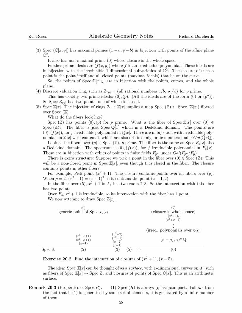
Zvi Rosen Algebraic Geometry Notes Richard Borcherds
(3) Spec (C[x, y]) has maximal primes (x− a, y− b) in bijection with points of the affine planeC2.
It also has non-maximal prime (0) whose closure is the whole space.Further prime ideals are (f(x, y)) where f is an irreducible polynomial. These ideals are
in bijection with the irreducible 1-dimensional subvarieties of C2. The closure of such apoint is the point itself and all closed points (maximal ideals) that lie on the curve.
So, the points of Spec C[x, y] are in bijection with the points, curves, and the wholeplane.
(4) Discrete valuation ring, such as Z(p) = {all rational numbers a/b, p 6 | b} for p prime.This has exactly two prime ideals: (0), (p). (All the ideals are of the form (0) or (pn)).
So Spec Z(p) has two points, one of which is closed.(5) Spec Z[x]. The injection of rings Z ↪→ Z[x] implies a map Spec (Z) ← Spec (Z[x]) fibered
over Spec (Z).What do the fibers look like?Spec (Z) has points (0), (p) for p prime. What is the fiber of Spec Z[x] over (0) ∈
Spec (Z)? The fiber is just Spec Q[x] which is a Dedekind domain. The points are(0), (f(x)), for f irreducible polynomial in Q[x]. These are in bijection with irreducible poly-nomials in Z[x] with content 1, which are also orbits of algebraic numbers under Gal(Q/Q).
Look at the fibers over (p) ∈ Spec (Z), p prime. The fiber is the same as Spec Fp[x] alsoa Dedekind domain. The spectrum is (0), (f(x)), for f irreducible polynomial in Fp(x).These are in bijection with orbits of points in finite fields Fpn under Gal(Fpn/Fp).
There is extra structure: Suppose we pick a point in the fiber over (0) ∈ Spec (Z). Thiswill be a non-closed point in Spec Z[x], even though ti is closed in the fiber. The closurecontains points in other fibers.
For example, Pick point (x2 + 1). The closure contains points over all fibers over (p).When p = 2, (x2 + 1) = (x+ 1)2 so it contains the point (x− 1, 2).
In the fiber over (5), x2 + 1 in F5 has two roots 2, 3. So the intersection with this fiberhas two points.
Over F3, x2 + 1 is irreducible, so its intersection with the fiber has 1 point.We now attempt to draw Spec Z[x].
(0)
generic point of Spec F2(x)
(0)
(closure is whole space)(x2+1),
(x3+x+1),
...(irred. polynomials over Q[x])
(x3+x+1)(x2+x+1)
(x−1)
(x2+2)(x2+1)(x−2)(x−1)
(x− a), a ∈ Q
Spec Z (2) (3) (5) · · · (0)
Exercise 20.2. Find the intersection of closures of (x2 + 1), (x− 5).
The idea: Spec Z[x] can be thought of as a surface, with 1-dimensional curves on it: suchas fibers of Spec Z[x]→ Spec Z, and closures of points of Spec Q[x]. This is an arithmeticsurface.
Remark 20.3 (Properties of Spec R). (1) Spec (R) is always (quasi-)compact. Follows fromthe fact that if (1) is generated by some set of elements, it is generated by a finite numberof them.
58

Zvi Rosen Algebraic Geometry Notes Richard Borcherds
(2) Every irreducible set is the closure of some point. (Exercise) There is a 1 : 1 correspondencebetween irreducible closed sets and points of Spec.
20.1. Local ringed structure of Spec (R). We need to assign a ring to every open subset. Recalllocalization of a ring R at some multiplicative subset S.
A multiplicative subset is defined as a set closed under multiplication (If S is not multiplicativejust replace it by the multiplicative subset it generates.)
Localization is the ring obtained from R by forcing all elements of S to be invertible.Construction: Take ring R[t1, t2, . . .] with ti corresponding to elements s1, s2, . . . of S.Then take the quotient R[t1, . . .]/(t1s1 − 1, t2s2 − 1, . . .). The obvious universal property is that
any homomorphism from R to any ring T so that the images of S are invertible factors uniquelythrough the localization.
Problem 20.4. We have a homomorphism R→ RS . What is its kernel?
If s ∈ S is a zerodivisor, i.e. sr = 0, then r ∈ kernel.If s is nilpotent, then the kernel is the whole ring, so the localization is the 0 ring.
Concrete construction of localization:Recall the ring of fractions of Z. The set of points (a, b), b 6= 0; we write these as a/b. We mod
out be the equivalence relations a/b = c/d if ad = bc. This suggests a definition for localizationRS . Look at pairs a/b such that b ∈ S.
We want to mod out by the equivalence relation a/b = c/d if bc = ad — however, if S containszerodivisors this will make a mess. The modified relation is: a/b ≡ c/d if s(ad − bc) = 0 for somes ∈ S. This complication is only needed if S has zerodivisors.
Now, check that this gives localization RS . (Long series of boring checks.)The advantage of the explicit construction of RS is that we can identify the kernel of R → RS .
Since a 7→ a/1, the equivalence relation tells us that a/1 = 0/1 when s(a − 0) = sa = 0 for somes ∈ S. Therefore, the kernel is the set of elements in R annihilated by some s ∈ S.
Recall, Spec R has a basis of open sets Df = prime ideals not containing f ∈ R (places wheref 6= 0).
Let O(Df ) = localization of R at f = R[f−1], where O(Df ) is the ring of the locally ringedspace associated to the open set Df .
Problem 20.5. What about the open sets U not of the form Df?
Bad news: O(U) is hard to describe explicitly.Good news: No need to describe O(U). Key point: We can construct sheaves by giving their
values on a basis for the topology, and checking the sheaf axioms for covers by sets in this basis.Suppose {Ui}i∈I form a basis fro the topology and we have groups S(Ui), maps S(Ui)→ S(Uj)
whenever Uj ⊆ Ui compatible for Ui ⊆ Uj ⊆ Uk. Suppose these satisfy the sheaf axiom for allcovers of some Ui by sets Uj , Uk, . . .
Then: S can be extended uniquely to a sheaf. The proof is left as an exercise.
Remark 20.6. The key philosophy for working with sheaves on Spec (R): Concentrate on theopen sets Df and ignore other open sets.
Example 20.7. In Spec k[x, y], the open sets x 6= 0, y 6= 0 has union A2 \ 0, not of the form Df .
Problem 20.8. We need to check the sheaf axioms for open sets Df . That is, suppose Df iscovered by open sets Df1 , Df2 , . . .– we want to show that given elements in O(Df1),O(Df2), . . .,there is a unique element in Df restricting to them all.
59

Zvi Rosen Algebraic Geometry Notes Richard Borcherds
Simplifications: 1. Replace the ring R by Rf so we can assume f = 1. So, Spec (R) coveredby Df1 , Df2 , . . . means that f1, f2, . . . generate the unit ideal in R. So, 1 = a1f1 + a2f2 + · · · forsome ai.
First check that r ∈ R is determined uniquely by its restrictions to the open sets Dfi . Supposer has image 0 in Dfi – what does this mean? R → Rfi then r ∈kernel if and only if fni
i r = 0 forsome ni, since the multiplicative subset is generated by fi.
So we want to show that if:
1 = a1f1 + a2f2 + · · · and fn11 r = 0, fn2
2 r = 0, . . .
then r = 0.Trick: Replace each fi by fni
i = gi. Then there is still a relation 1 = b1g1 + b2g2 + · · · for some
bi as 1 = (a1f1 + · · · )N , and for N sufficiently large, every term in this expansion is divisible byone of fni
i . So we have 1 = b1g1 + b2g2 + · · · , and g1r = 0, g2r = 0. Multiplying both sides of thefirst equation by r and substituting, we find r = 0.
Hard part: Suppose we have compatible elements ri/fnii in O(Dfi) = Rfi . We need to find r ∈ R
whose image in Rfi is ri/fnii .
What do we mean by compatible elements? That ri/fnii and rj/f
nj
j are the same in Rfifj . Thismeans:
(fifj)mij (rif
nj
j − rjfnii ) = 0
for some mij .As before, we have 1 = a1f1 + a2f2 + · · · for some ai. We want to find r = r/1 with
fmii (fni
i r − ri) = 0
for some mi. We need to solve this equation, which we will do next time.
21. Thursday, November 15, 2012
21.1. Spec R is a sheaf. Last time we were discussing the Construction of Spec (R). So far:
• Points are prime ideals of R.• Base for open sets: Df , (f ∈ R) = prime ideals not containing f . “Points where f 6= 0.”• Ringed Structure: O(Df ) = R[f−1] for each f .
We need to check sheaf property whenever Df is covered by open sets Dfi .Step 1: We can assume f = 1 by replacing R with Rf .We are given 1 = a1f1 + · · · , where Dfi cover Spec R.Assuming that r is in the kernel of the localization, there exists mij such that
fmij
i fmij
j (rifnj
j − rjfnii ) = 0
This implies thatrifnii
=rj
fnj
j
on Dfi ∩Dfj .
We want to find r ∈ R such that fkii (fnii r − ri) = 0. This is hard to solve directly.
The result isrifnii
= ron Dfi .
We replace fi by suitable powers of fi. Then, we can assume that 1 = a1f1 + a2f2 + · · · suchthat fifj(rifj − rjfi) = 0. We want to find r with fi(fir − ri) = 0. Now we replace rifi by si.
We get 0 = sif2j − sif2
i . We have to solve f2i r = si. Again we replace by f2
i by gi, so 1 =b1g1 + b2g2 + · · · for some bi’s.
We have reduced to the following problem: Given 1 = b1g1 + b2g2 + · · · such that sigj = sjgi wewant to solve, gir = si.
60

Zvi Rosen Algebraic Geometry Notes Richard Borcherds
Remark 21.1. Motivation: What is r? Suppose gir = si. Then r = r · 1 = rb1g1 + rb2g2 + · · · =b1s1 + b2s2 + · · · .
So we define r to be b1s1 + b2s2 + · · · . Now it is easy to check that gir = si.
Remark 21.2. Key properties of Spec R:
(1) O(Df ) = R[f−1] for f ∈ R.(2) Local ring at p ∈ Spec R = Rp = localization of R at p = RS where S is the complement of
p, which is multiplicative.You can also consider this as the
limp∈UO(U) = lim
p∈Df
O(Df ) = limf /∈p
R[f−1] = Rp.
(3) Ignore open sets not of the form Df .
Definition 21.3. A scheme is a ringed space locally isomorphic to Spec (commutative ring). Thisis a locally ringed space: localization at any points is a local ring.
Remark 21.4. Two different concepts: Morphisms of ringed spaces and morphisms of locallyringed spaces f : X → Y are NOT the same.
Morphisms of locally ringed spaces (informally) are morphisms such that a function g on Yvanishes at a point y ∈ Y its pullback should vanish at f−1(y). Rephrase this in terms of ringedspace structure.
Definition 21.5. Morphism of ringed spaces X → Y consists of
(1) Continuous map f from X to Y .(2) If U ⊂ Y , we need to be given a morphism of rings O(U)→ O(f−1U).(3) Should satisfy various compatibility conditions.
For locally ringed spaces, we need to add the extra condition:If y ∈ Y and f(x) = y, we get a homomorphism:
(local ring at y) → (local ring at X)
This is a homomorphism of local rings, meaning it maps the maximal ideal of the first into themaximal ideal of the second.
Example 21.6. There are ringed space morphisms between locally ringed spaces that are notmorphisms of locally ringed spaces.
Take R = Z(p) = {m/n | p 6 | n}. (Alternatively, any discrete valuation ring), and Q = rationals= quotient field of R.
Spec Q = 1 point. O(Spec (Q)) = Q. Spec R has 2 points: (p) closed, (0) not closed.What about morphisms Spec Q→ Spec R. The obvious one, coming from R ⊂ Q takes a point
of Q to the open point of Spec R. Then f : R→ Q will have f((0)) = (0).This is a morphism of locally ringed spaces. The corresponding homomorphism of local rings is
just Q→ Q.Another morphism of ringed spaces is g which takes the point (0) ∈ Spec Q to the point (p) in
Spec R.g : Spec (Q)→ Spec R. We need to define the map from O(Spec R)→ O(Spec Q). Look at the
effect on local rings, which is of course R ⊆ Q.Local ring of Spec R at closed point (p) is R. So we get a homomorphism of rings R ↪→ Q.
However this is not a hom. of local rings, since it does not map (p) ⊂ R into (0) ⊂ Q.
Reason for this:
Homomorphisms of rings from R→ S ←→ morphisms of locally ringed spaces from Spec S → Spec R.61

Zvi Rosen Algebraic Geometry Notes Richard Borcherds
Otherwise you would get morphisms of affine schemes not corresponding to morphisms of rings.So, the category of Rings is essentially the opposite of the category of affine schemes.Special case of the following: We can describe morphisms of any scheme to Spec (R) for R a
commutative ring. If X is a scheme and we have a morphism X → Spec (R), then in particular weget a homomorphism of rings from R to O(X). (R is the ring of the open set Spec (R)).
This is an isomorphism: maps of schemes X → Spec R are the “same” as homomorphisms ofrings from R to O(X).
Remark 21.7. Consequence of this fact: The definition of an affine scheme Spec R is correct.This isomorphism indicates a pair of adjoint functors:
Locally Ringed Spaces RingsX −→ O(X)
Spec R ←− R
These are unique up to equivalence. So, spec of a ring could be defined as adjoint functors of thenatural forgetful functor from locally ringed spaces to rings.
21.2. Constructing Schemes from Graded Rings.
(1) The points of Spec R are prime ideals.(2) Base of open sets are Df .(3) O(Df ) = R[f−1].
We can consider R as the local ring of an affine variety.Recall that a projective variety has a homogeneous coordinate ring R which is graded: R =
R0 ⊕R1 ⊕ · · · .From the homogeneous coordinate ring of a projective variety, we are able to construct the
projective variety. Similarly, we want to take any graded ring to a scheme Proj R.
Definition 21.8. (1) The points of Proj R are graded prime ideals, not containing all positivehomogeneous elements.
(2) Basis for the open sets: Df for f homogenous. This is graded prime ideals of Proj (R) notcontaining f . (informally) points where f does not vanish.
(3) Ringed space structure: O(Df ) = R[f−1]0.
Example 21.9. Take R = k[x0, . . . , xn]. Taking the graded prime deals corresponds to subvarietiesthat are cones.
Not containing all positive homogeneous elements corresponds to not being 0.So homogeneous primes not containing all pos. degree elements gives subvarieties of Pn.
Example 21.10. Let R = k[x0, . . . , xn]. Let f = x0. Then Df should be the affine spaceof all points (1 : x1 : · · · : xn). Coordinate ring will be k[x1, . . . , xn] = degree 0 elements ofk[x1, . . . , xn][x−1
0 ].
Moreover, the open subset Df is in fact an affine scheme Spec (Df ). So Proj R is covered byopen affine subschemes Spec Df for f homogeneous, so it is a scheme. (Left as exercise.)
As with affine schemes, we work with Df and ignore open sets of other types.
Remark 21.11. Given a scheme X, it determines a functor of points: a functor from schemes Sto sets taking S →Mor(S,X), where the latter set is called the S-valued points of X.
Example 21.12. Suppose X = affine scheme Spec R. Then the corresponding functor of pointstakes S to HomRings(R,O(S)).
For R = Z[x], the functor of points maps to Hom(R,O(S)) = O(S). So the functor of schemeSpec Z[x] takes any scheme to its ring of global functions.
62

Zvi Rosen Algebraic Geometry Notes Richard Borcherds
Now we look at the same question for Proj R. Given a scheme S, what are the morphisms fromS to Proj R?
Example 21.13. Let R = Z[x0, x1]. Proj R = projective line (over Z). Then, Mor(S,Proj R) =projective line over S.
Suppose S is an affine scheme Spec A. What are the points of the projective line over a ring A?For a field A, the answer is
(1) (x : y)/(x : y) ∼ (λx : λy) where x, y are not both 0.(2) Union of 2 affine lines (1 : y) ∪ (x : 1) glued together.
In general, both of these are wrong.
63