Working Paper No. 41

Fiscal policy in an endogenous growth model

with public capital and pollution

by

Alfred Greiner

University of Bielefeld

Department of Economics

Center for Empirical Macroeconomics

P.O. Box 100 131

33501 Bielefeld, Germany

Fiscal policy in an endogenous growth model with

public capital and pollution

Alfred Greiner∗

Abstract

In this paper we study growth and welfare effects of fiscal policy in an endogenous

growth model with public capital and environmental pollution. As to pollution we

assume that it is due to aggregate production. Pollution does not have direct effects

as concerns production possibilities but it only reduces utility of the household.

The paper then studies growth effects of fiscal policy for the model on the balanced

growth path and taking into account transition dynamics. Further, welfare effects

of fiscal policy are analyzed and it is demonstrated that the growth maximizing

values of tax rates may be different from those values which maximize the long run

balanced growth rate.

JEL: O41, Q38

Keywords: Fiscal Policy, Endogenous Growth, Public Capital, Environmental Pollution

∗Department of Economics, University of Bielefeld, P.O. Box 100131, 33501 Bielefeld, Germany.

1 Introduction

One strand in endogenous growth theory assumes that the government can invest in

productive public capital which stimulates aggregate productivity. This approach goes

back to Arrow and Kurz (1970) who presented exogenous growth models containing that

assumption in their book. The first model in which productive public spending leads to

sustained per capita growth in the long run was presented by Barro (1990). In his model,

productive public spending positively affects the marginal product of private capital and

makes the long run growth rate an endogenous variable. However, the assumption that

public spending as a flow variable affects aggregate production possibilities is less plausible

from an empirical point of view as pointed out in a study by Aschauer (1989).

Futagami et al. (1993) have extended the Barro model by assuming that public capital

as a stock variable shows positive productivity effects and then investigated whether the

results derived by Barro are still valid given their modification of the Barro model. As

to the question of whether public spending can affect aggregate production possibilities

at all the empirical studies do not reach unambiguous results. However, this is not too

surprising since these studies often consider different countries over different time periods

and the effect of public investment in infrastructure for example is likely to differ over

countries and over time. A good survey of the empirical studies dealing with that subject

can be found in Sturm et al. (1998).

Another line of research in economics are studies which try to understand the links

between economic growth and pollution. Basically, there are two different ways of in-

tegrating the environment in economic models. On the one hand, models have been

constructed in which economic activities generate environmental degradation. That line

of research goes back to Forster (1973) and was extended by Gruver (1976).

On the other hand, there are so-called resource models in which a stock of natural

resources is exploited in order to take up production. From the technical point of view, an

equivalent formulation is the assumption that economic activities lead to pollution which

1

negatively affects the environmental quality. Models of this type within an endogenous

growth framework are for example in the papers by Bovenberg and Smulders (1995) or

Gradus and Smulders (1993)1.

Most of the models dealing with environmental quality or pollution assume that pol-

lution or the use of resources influences prodution possibilities either through affecting

the accumulation of human capital or by directly entering the production function. In

this paper we pursue a different approach. We intend to analyze a growth model where

pollution only affects utility of a representative household but does not affect production

possibilities directly by entering the aggregate production function. However, there is

an indirect effect of pollution on output because we suppose that resources are used for

abatement activities. As concerns pollution we assume that it is an inevitable by-product

of production and that it can be reduced to a ceratin degree by investing in abatement

activities. As to the growth rate we suppose that it is determined endogenously and that

public investment in a productive public capital stock brings about sustained long run

per capita growth. Thus, we adopt that type of endogenous growth models which was

initiated by Barro (1990) and Futagami et al. (1993) we mentioned above.

Within this framework we intend to analyze how the long run balanced growth rate

reacts to fiscal policy and to the introduction of a less polluting technology. Further,

we also study the effects of fiscal policy taking into account transition dynamics and we

analyze welfare effects of fiscal policy for the model on the balanced growth path.

The rest of the paper is organized as follows. In section 2 we present the structure

of our model and in section 3 we solve the model and show that there exists a unique

balanced growth path. Section 4 analyzes growth effects of fiscal policy and growth effects

of introducing a cleaner production technology for our model on the balanced growth path.

Further, we also study the effects of fiscal policy as to the growth rates on the transition

path. In section 5 we analyze welfare effects and section 6 concludes the paper.

1For a good survey of how to model pollution in growth models see Smulders (1995) or Hettich (2000).

2

2 The economic model

We consider an economy with a household sector, a productive sector, and the government.

First, we describe the household sector.

2.1 The household

Our economy is represented by one household. The goal of this household is to maximize

a discounted stream of utility arising from consumption C(t) over an infinite time horizon

subject to its budget constraint:

maxC(t)

∫

∞

0e−ρtV (t)dt, (1)

with V (t) the instantaneous subutility function which depends positively on the level

of consumption and negatively on effective pollution. V (t) takes the logarithmic form

V (t) = ln C(t) − ln PE(t), with ln giving the natural logarithm.2 ρ in (1) gives the

subjective discount rate.

The budget constraint is given by3

K = (w + rK)(1 − τ) − C. (2)

The budget constraint (2) states that the individual has to decide how much to consume

and how much to save, thus increasing consumption possibilities in the future. The

depreciation of physical capital is assumed to equal zero.

w in the budget constraint is the wage rate. The labour supply L is constant, supplied

inelastically, and we normalize L ≡ 1. r is the return to per capita capital K and τ ∈ (0, 1)

gives the income tax rate.

To derive necessary conditions we formulate the Hamiltonian function as H(·) = ln C−

ln PE + λ(−C + (w + rK)(1− τ)), with λ the costate variable. The necessary optimality

2For a survey of how to incorporate pollution in the utility function see Smulders (1995), p. 328-29.

3In what follows we will suppress the time argument if no ambiguity arises.

3

conditions are given by

λ = C−1, (3)

λ/λ = ρ − r(1 − τ), (4)

K = −C + (w + rK)(1 − τ). (5)

Since the Hamiltonian is concave in C and K jointly, the necessary conditions are also

sufficient if in addition the transversality condition at infinity limt→∞ e−ρtλ(t)K(t) ≥ 0 is

fulfilled. Moreover, strict concavity in C also guarantees that the solution is unique (cf.

Seierstad and Sydsaeter (1987), pp. 234-235).

2.2 The productive sector

The productive sector in our economy is represented by one firm which chooses inputs

in order to maximize profits and which behaves competitively. As to pollution P (t), we

suppose that it is a by-product of aggregate production Y . In particular, we assume that

P (t) = ϕY (t), with ϕ = const. > 0. Thus, we follow the line invited by Forster (1973)

and worked out in more details by Luptacik and Schubert (1982).

Effective pollution PE which affects utility of the household is that part of pollution

which remains after investing in abatement activities. This means that abatement activ-

ities reduce pollution but cannot eliminate it completely. As to the modeling of effective

pollution we follow Gradus and Smulders (1993) and Lighthart and van der Ploeg (1994)

and take the following specification

PE =P

Aβ, 0 < β ≤ 1. (6)

The limitation β ≤ 1 assures that a positive growth rate of aggregate production goes

along with an increase in effective pollution, β < 1, or leaves effective pollution unchanged,

β = 1. We make that assumption because we think that it is realistic to assume that

higher production also leads to an increase in pollution, although at a lower rate because

of abatement. Looking at the world economy that assumption is certainly justified.

4

Pollution is taxed at the rate τp > 0 and the firm takes into account that one unit of

output causes ϕ units of pollution for which it has to pay τpϕ per unit of output. The

per capita production function is given by,

Y = KαH1−α, (7)

with H denoting the stock of productive public capital and α ∈ (0, 1) gives the per capita

capital share. Recall that K denotes per capita capital and that L is normalized to one.

Assuming competitive markets and taking public capital as given the first-order con-

ditions for a profit maximum are obtained as

w = (1 − τpϕ)(1 − α)KαH1−α, (8)

r = (1 − τpϕ)αKα−1H1−α. (9)

2.3 The government

The government in our economy uses resources for abatement activities A(t) which reduce

total pollution. Abatement activities A ≥ 0 are financed by the tax revenue coming from

the tax on pollution, i.e. A(t) = ητpP (t), with η > 0. If η < 1 not all of the pollution

tax revenue is used for abatement activities and the remaining part is spent for public

investment in the public capital stock Ip, Ip ≥ 0, in addition to the tax revenue resulting

from income taxation. For η > 1 a certain part of the tax revenue resulting from the

taxation of income is used for abatement activities in addition to the tax revenue which

is gained by taxing pollution. As to the interpretation of public capital one can think of

pure public like infrastructure capital. However, one could also interpret public capital

in a broader sense so that it also includes human capital which is built up as a result of

public education.

The government in our economy runs a balanced budget at any moment in time. Thus,

the budget constraint of the government is written as

Ip = τpP (1 − η) + wτw + rKτK . (10)

5

The evolution of public capital is described by

H = Ip, (11)

where for simplicity we again assume that there is no depreciation of public capital. As

to the governmental decision rules, we do not try to find out the second best optimal

level for the tax rates or the amount of abatement activities nor the socially optimal

decisions for consumption and the fiscal parameters. Instead, we only consider how the

growth rate reacts to changes in fiscal policy. This seems to be of higher relevance for

real world economies with a democratic government because government behaviour may

be hampered by bureaucracy and by political or institutional constraints (as to this ar-

gumentation see also van Ewijk and van de Klundert (1993)).

3 Equilibrium conditions and the balanced growth

path

Combining the budget constraint of the government and the equation describing the

evolution of public capital over time, the accumulation of public capital can be written

as H = −ηϕτpKαH1−α + τpϕKαH1−α + τ(w + rK) = KαH1−α(ϕτp(1− η) + (1− ϕτp)τ),

where we have used (8) and (9). To obtain the other differential equations describing our

economy we note that the growth rate of private consumption is obtained from (3) and

(4), with r taken from (9) and where we have used PE/PE = (1 − β)Y /Y. Using (8) and

(9) K/K is obtained from (5). It should be noted that the accumulation of public capital

which is positive for Ip > 0 is the source of sustained economic growth in our model and

makes the growth rate an endogenous variable.

Thus, the dynamics of our model are completely described by the following differential

equation system:

C

C= −ρ + (1 − τ)(1 − ϕτp) α

(

H

K

)1−α

, (12)

6

K

K= −

C

K+(

H

K

)1−α

(1 − ϕτp) (1 − τ) , (13)

H

H=

(

H

K

)−α

(ϕτp (1 − η) + (1 − ϕτp) τ) . (14)

The initial conditions K(0) and H(0) are given and fixed and C(0) can be chosen freely

by the economy. Further, the transversality condition limt→∞ e−ρtK(t)/C(t) ≥ 0 must be

fulfilled.

In the following we will first examine our model as to the existence and stability of a

balanced growth growth (BGP). To do so, we define a BGP.

Definition A balanced growth path (BGP) is a path such that C/C = K/K = H/H ≡

g > 0 holds, with g constant and C, K and H strictly positive.

This definition shows that on a BGP the growth rates of economic variables are positive

and constant over time. It should be noticed that aggregate output and pollution grow

at the same rate on the BGP. This implies that effective pollution is not constant in the

long run (unless β = 1 holds). Nevertheless, one may say that the BGP is sustainable

if one adopts the definition given in Byrne (1997). There, sustainable growth is given

if V is positive. For our model this holds on the BGP since V = C/C − PE/PE =

C/C − (1 − β)Y /Y = βg > 0.

To analyze our model further, we first have to perform a change of variables. Defining

c = C/K and h = H/K and differentiating these variables with respect to time we get

c/c = C/C − K/K and h/h = H/H − K/K. A rest point of this new system then

corresponds to a BGP of our original economy where all variables grow at the same

constant rate. The system describing the dynamics around a BGP is given by

c = c(

c − ρ − (1 − α)(1 − τ)(1 − ϕτp)h1−α

)

, (15)

h = h(

c − h1−α(1 − ϕτp)(1 − τ) + h−α(ϕτp(1 − η) + (1 − ϕτp)τ))

. (16)

Concerning a rest point of system (15) and (16) it should be noted that we only consider

interior solution. That means that we exclude the economically meaningless stationary

7

point c = h = 0. As to the uniqueness and stability of a BGP we can state proposition 1.

Proposition 1 Assume that τpϕ < 1 and (1− τpϕ)τ + (1− η)τpϕ > 0. Then there exists

a unique BGP which is saddle point stable.

Proof: To prove that proposition we first calculate c∞ on a BGP which is obtained from

h/h = 0 as

c∞ = h1−α(1 − ϕτp)(1 − τ) − h−α(ϕτp(1 − η) + (1 − ϕτp)τ).

Inserting c∞ in (15) gives after some modifications

f(·) ≡ c/c = −ρ + (1 − τ)(1 − ϕτp)αh1−α − h−α(ϕτp(1 − η) + (1 − ϕτp)τ),

with limh→0 f(·) = −∞ (for Ip > 0) and limh→∞ f(·) = ∞. A rest point for f(·), i.e. a

value for h such that f(·) = 0 holds, then gives a BGP for our economy. Further, we have

∂f(·)/∂h = (1 − τ)(1 − ϕτp)(1 − α)αh−α + αh−α−1(ϕτp(1 − η) + (1 − ϕτp)τ) > 0,

for Ip > 0. Note that on a BGP H/H > 0 must hold implying Ip > 0 and, thus,

ϕτp(1 − η) + (1 − ϕτp)τ > 0. ∂f/∂h > 0 for h such that f(·) = 0 means that f(·) cannot

intersect the horizontal axis from above. Consequently, there exists a unique h∞ such

that f(·) = 0 and, therefore, a unique BGP.

The saddle point property is shown as follows. Denoting with J the Jacobi matrix

of (15) and (16) evaluated at the rest point we first note that det J < 0 is a necessary

and sufficient condition for saddle point stability, i.e. for one negative and one positive

eigenvalue. The Jacobian in our model can be written as

J =

c −c h−α(1 − α)2(1 − τ)(1 − τpϕ)

h −υ

,

with

υ = (1 − α)h1−α(1 − τ)(1 − τpϕ) + αh−α(ϕτp(1 − η) + (1 − ϕτp)τ).

8

The determinant can be calculated as

det J = −c hα(

h−α−1(ϕτp(1 − η) + (1 − ϕτp)τ) + (1 − α)h−α(1 − τ)(1 − τpϕ))

< 0.

Thus, proposition 1 is proved. 2

That proposition states that our model is both locally and globally determinate, i.e.

there exists a unique value for c(0) such that the economy converges to the BGP in the long

run.4 The asumption (1−ϕτp) > 0 is necessary for a positive growth rate of consumption

and is sufficient for a positive value of c∞.5 The second assumption (ϕτp(1 − η) + (1 −

ϕτpτ) > 0 must hold for a positive growth rate of public capital. It should be noted that

(ϕτp(1 − η) + (1 − ϕτpτ)) = Ip/Y stating that the second assumption in proposition 1

means that on a BGP the ratio of public investment to GDP must be positive.

4 Growth effects of fiscal policy

In the last section we demonstrated in proposition 1 that there is a unique BGP under

slight additional assumptions. Thus our model including the transition dynamics is com-

pletely characterized. In this section we will analyze how the growth rate in our economy

reacts to fiscal policy. We do this for the model on the BGP and taking into account

transition dynamics.

4.1 The BGP

Before we analyze growth effects of fiscal policy we study effects of introducing a less

polluting production technology, i.e. the impact of a decline in ϕ.

The balanced growth rate which we denote with g is given by (14) as

g = H/H = (h)−α (ϕτp(1 − η) + (1 − ϕτp)τ) .

4For a definition of local and global determinacy see e.g. Benhabib and Perli (1994) or Benhabib,

Perli, and Xie (1994).

5This is realized if c∞ is calculated from c/c = 0 as c∞ = ρ + (1 − α)(1 − τ)(1 − τpϕ)h1−α.

9

Differentiating g with respect to ϕ gives

∂g

∂ϕ= h−ατp(1 − η − τ) − (ϕτp(1 − η) + (1 − ϕτp)τ)αh−α−1 ∂h

∂ϕ.

∂h/∂ϕ is obtained by implicit differentiation from f(·) = 0 (from the proof of proposition

1) as∂h

∂ϕ=

τp(1 − η − τ) + τp(1 − τ)αh

α(1 − τ)(1 − ϕτp)(1 − α) + αh−1(ϕτp(1 − η) + (1 − ϕτp)τ).

For (1− η − τ) = 0 we get ∂g/∂ϕ < 0. To get results for (1− η − τ) 6= 0 we insert ∂h/∂ϕ

in ∂g/∂ϕ. That gives

∂g

∂ϕ= h−ατp(1 − η − τ) ·

(

1 −(ϕτp(1 − η) + (1 − ϕτp)τ)[(1 − η − τ) + hα(1 − τ)]

(1 − η − τ)[(ϕτp(1 − η) + (1 − ϕτp)τ) + h(1 − τ)(1 − τpϕ)(1 − α)]

)

.

From that expression it can be seen that the expression in brackets is always positive for

(1 − η − τ) < 0 such that ∂g/∂ϕ < 0. For (1 − η − τ) > 0 it is immediately seen that

∂g

∂ϕ> = < 0 ⇔ (1 − ϕτp)(1 − α)(1 − η − τ) > = < α (ϕτp(1 − η) + (1 − ϕτp)τ),

which simplifies to

∂g

∂ϕ> = < 0 ⇔ (1 − η)(1 − α) > = < ϕτp(1 − η) + (1 − ϕτp)τ.

The r.h.s. of that expression is equivalent to IP /Y. Thus we have proved the following

proposition.

Proposition 2 If (1−η−τ) ≤ 0 the use of a less polluting technology raises the balanced

growth rate. For (1 − η − τ) > 0 the use of a less polluting technology raises (leaves

unchanged, lowers) the balanced growth rate if

Ip

Y> (=, <)(1 − α)(1 − η).

10

To interpret that result we first note that a cleaner production technology (i.e. a lower ϕ)

shows two different effects: on the one hand it implies that less resources are needed for

abatement activities leaving more resources for public investment. That effect leads to a

higher ratio H/K, thus raising the marginal product of private capital r in (9). That is

the return on investment rises. Further, a less polluting technology implies that the firm

has to pay less pollution taxes (the term (1 − τpϕ) rises) which has also a stimulating

effect on r, which can be seen from (9) and which also raises the incentive to invest. On

the other hand, however, less pollution implies that the tax revenue resulting from the

taxation of pollution declines and, thus, productive public spending. That effect tends to

lower the ratio H/K and, therefore, the marginal product of private capital. This tends

to lower the balanced growth rate.

If η ≥ 1− τ, i.e. if much of the pollution tax is used for abatement activities a cleaner

technology always raises the balanced growth rate. In that case, the negative growth

effect of a decline in the pollution tax revenue is not too strong since most of that revenue

is used for abatement activities which are non-productive anyway. If, however, η < 1− τ,

i.e. a good deal of the pollution tax is used for productive government spending, a cleaner

technology may either raise or lower economic growth. It increases the balanced growth

rate if the share of public investment per GDP is larger than a constant which positively

depends on the elasticity of aggregate output with respect to public capital and negatively

on η, and vice versa.

Let us next study growth effects of varying the income tax rate. Proposition 3 demon-

strates that a rise in that tax may have positive or negative growth effects and that there

exists a growth maximizing income tax rate.

Proposition 3 Assume that there exists an interior growth maximizing income tax rate.

Then this tax rate is given by

τ = (1 − α) − αϕτp(1 − η)/(1 − ϕτp).

Proof: To calculate growth effects of varying τ we take the balanced growth rate g from

11

(14) and differentiate it with respect to that parameter. Doing so gives

∂g

∂τ= h−α(1 − τpϕ)

(

1 −α((1 − τpϕ)τ + (1 − η)τpϕ)

1 − τpϕ

∂h

∂τ

1

h

)

,

where ∂h/∂τ is obtained by implicit differentiation from f(·) = 0 leading to

∂h

∂τ=

(1 − ϕτp)(1 + α h)h

h(1 − τ)(1 − ϕτp)(1 − α)α + α((1 − τpϕ)τ + (1 − η)τpϕ).

Inserting ∂h/∂τ in ∂g/∂τ we get

∂g

∂τ= h−α(1 − τpϕ)

(

1 −((1 − τpϕ)τ + (1 − η)τpϕ)(1 + α h)

h(1 − τ)(1 − ϕτp)(1 − α) + ((1 − τpϕ)τ + (1 − η)τpϕ)

)

,

showing that

∂g

∂τ> = < 0 ⇔ (1 − τ)(1 − ϕτp)(1 − α) > = < α((1 − τpϕ)τ + (1 − η)τpϕ).

Solving for τ gives

∂g

∂τ> = < 0 ⇔ τ < = > (1 − α) − αϕτp(1 − η)/(1 − ϕτp)

That shows that the balanced growth rate rises with increases in τ as long as τ is smaller

than the expression on the r.h.s. which is constant. 2

That proposition shows that the growth maximizing income tax rate does not neces-

sarily equal zero in our model which was to be expected since the government finances

productive public spending with the tax revenue. There are two effects of going along

with variations of the income tax rate: on the one hand, a higher income tax lowers the

marginal product of private capital and, therefore, is a disincentive for investment. On

the other hand, the government finances productive public spending with its tax revenue

leading to a rise in the ratio H/K, which raises the marginal product of private capital r

and which has, as a consequence, a positive effect on economic growth. However, bound-

ary solutions, i.e. τK = 0 or τK = 1, cannot be excluded. Whether there exists an interior

or a boundary solution for the growth maximizing capital income tax rate depends on

the numerical specification of the parameters ϕ, τp, and η. Only for ϕτp = 0 or η = 1 the

12

growth maximizing tax rate is always in the interior of (0, 1) and equal to the elasticity

of aggregate output with respect to public capital.

As to the tax on pollution the growth maximizing income tax rate negatively varies

with that tax if η < 1. For η > 1 the growth maximizing income tax rate is the higher

the higher the tax on pollution τp. The interpretation of that result is as follows: if η < 1

the government uses a part of the pollution tax revenue for the creation of public capital

which has positive growth effects. Increasing the tax on pollution implies that a part of the

additional tax revenue is used for productive investment in public capital. Consequently,

the income tax rate can be reduced without having negative growth effects. It should be

noticed that a decrease in the income tax rate shows an indirect positive growth effect

because it implies a reallocation of private resources from consumption to investment. In

contrast to that, if η > 1 the whole pollution tax revenue is used for abatement activities.

Raising the pollution tax rate in that situation implies that the additional tax revenue is

used only for abatement activities but not for productive public spending. Consequently,

the negative indirect growth effect of a higher pollution tax (through decreasing the return

on capital r) must be compensated by an increase in the income tax rate. It should be

noted that the latter also has a negative indirect growth effect but that one is dominated

in this case by the positive direct growth effect of higher productive public spending.

Let us next analyze long run growth effects of a rise in the pollution tax rate. Propo-

sition 4 gives the result.

Proposition 4 For (1 − η − τ) ≤ 0 a rise in the pollution tax rate always lowers the

balanced growth rate. If (1 − η − τ) > 0 the pollution tax rate maximizing the balanced

growth rate is determined by

τp =

(

1

ϕ

)(

1 − η − τ − α(1 − η)

1 − η − τ

)

which is equivalent to

Ip

Y= (1 − α)(1 − η).

13

Proof: To calculate growth effects of varying τp we take the balanced growth rate g again

from (14) and differentiate it with respect to that parameter. Doing so gives

∂g

∂τp

= h−αϕ(1 − η − τ) ·

(

1 −(ϕτp(1 − η) + (1 − ϕτp)τ)[(1 − η − τ) + hα(1 − τ)]

(1 − η − τ)[(ϕτp(1 − η) + (1 − ϕτp)τ) + h(1 − τ)(1 − τpϕ)(1 − α)]

)

.

From that expression it can be seen that the expression in brackets is always positive for

(1 − η − τ) < 0 such that ∂g/∂τp < 0. For (1 − η − τ) = 0 the result can directly be seen

by multiplying out the expression above. For (1 − η − τ) > 0 it is seen that

∂g

∂τp

> = < 0 ⇔ (1 − ϕτp)(1 − α)(1 − η − τ) > = < α (ϕτp(1 − η) + (1 − ϕτp)τ),

which simplifies to

∂g

∂τp

> = < 0 ⇔ τp < = >

(

1

ϕ

)(

1 − η − τ − α(1 − η)

1 − η − τ

)

and is equivalent to

∂g

∂τp

> = < 0 ⇔Ip

Y< = > (1 − η)(1 − α).

Thus, the proposition is proved. 2

The interpretation of that result is straightforward. An increase in the pollution tax

rate always lowers the balanced growth rate if (1 − η − τ) ≤ 0. In that case, too much of

the additional tax revenue (gained through the increase in τp) goes in abatement activities

so that the positive growth effect of a higher pollution tax revenue (i.e. the increase in

the creation of the stock of public capital) is dominated by the negative indirect one of

a reduction of the rate of return to physical capital r. The latter effect namely implies a

reallocation of private resources from investment to consumption which reduces economic

growth. For (1 − η − τ) > 0, however, there exists a growth maximizing pollution tax

rate.6 In that case, the pollution tax has to be set such that public investment per GDP

6But it must kept in mind that 1− τpϕ > 0 must hold so that a BGP exists. Therefore, the boundary

condition τp = ϕ−1 − ε, ε > 0, cannot be excluded.

14

equals the elasticity of aggregate output with respect to public capital multiplied with

that share of the pollution tax revenue which is not used for abatement activities but for

productive public spending.

Further, it should be noticed that the growth maximizing value of τp7 is the higher

the less of the pollution tax revenue is used for abatement activities. In the limit (η = 0)

we get the same result as in Barro (1990) and Futagami et al. (1993) that the growth

maximizing share of public investment per GDP equals the elasticity of aggregate output

with respect to public capital.

It should also be noted that the conditions for a positive growth effect of an increase

in the pollution tax rate are just reverse to the conditions which must be fulfilled such

that the introduction of a less polluting technology raises economic growth.

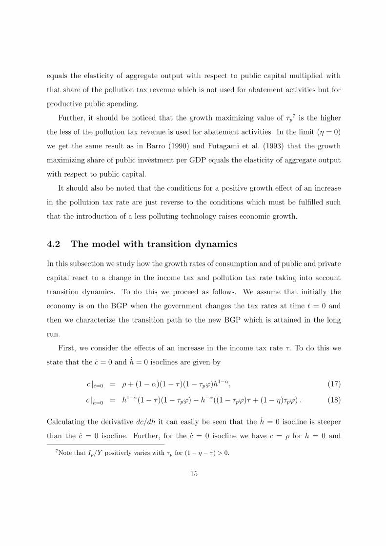
4.2 The model with transition dynamics

In this subsection we study how the growth rates of consumption and of public and private

capital react to a change in the income tax and pollution tax rate taking into account

transition dynamics. To do this we proceed as follows. We assume that initially the

economy is on the BGP when the government changes the tax rates at time t = 0 and

then we characterize the transition path to the new BGP which is attained in the long

run.

First, we consider the effects of an increase in the income tax rate τ. To do this we

state that the c = 0 and h = 0 isoclines are given by

c |c=0 = ρ + (1 − α)(1 − τ)(1 − τpϕ)h1−α, (17)

c |h=0 = h1−α(1 − τ)(1 − τpϕ) − h−α((1 − τpϕ)τ + (1 − η)τpϕ) . (18)

Calculating the derivative dc/dh it can easily be seen that the h = 0 isocline is steeper

than the c = 0 isocline. Further, for the c = 0 isocline we have c = ρ for h = 0 and

7Note that Ip/Y positively varies with τp for (1 − η − τ) > 0.

15

c → ∞ for h → ∞. For the h = 0 isocline we have c → −∞ for h → 0, c = 0 for

h = ((1− τpϕ)τ + (1− η)τpϕ)/((1− τ)(1− τpϕ)) and c → ∞ for h → ∞. This shows that

there exists a unique (c∞, h∞) where the two isoclines intersect.

If the income tax rate is increased it can immediately be seen that the h = 0 isocline

shifts to the right and the c = 0 isocline turns right with c = ρ for h = 0 remaining

unchanged. This means that both on the new c = 0 and on the new h = 0 isocline any

given h goes along with a lower value of c compared to the isoclines before the tax rate

increase. This implies that the increase in the income tax rate raises the long run value

h∞ and may reduce or raise the long run value of c∞. Further, the capital stocks K and

H are predetermined variables which are not affected by the tax rate increase at time

t = 0. These variables react only gradually. This implies that ∂h(t = 0, τ)/∂τ = 0. To

reach the new steady state8 (c∞, h∞) the level of consumption adjusts and jumps to the

stable manifold implying ∂c(t = 0, τ)/∂τ < 0 in figure 1.

Figure 1 about here

Over time both c and h rise until the new BGP is reached at (c∞, h∞). That is we get

c/c = C/C−K/K > 0 and h/h = H/H−K/K > 0 implying that on the transition path

the growth rates of consumption and of public capital are larger than that of private capital

for all t ∈ [0,∞). The impact of a rise in τ on the growth rate of private consumption is

obtained from (12) as

∂

∂τ

(

C(t = 0, τ)

C(t = 0, τ)

)

= −h1−αα(1 − τpϕ) < 0,

where we again use that K and H are predetermined variables implying ∂h(t = 0, τ)/∂τ =

0. This shows that at t = 0 the growth rate of private consumption reduces as a result

of the increase in the income tax rate τ and then rises gradually as the new BGP is

approached. The same must hold for the private capital stock since we know from above

8The economy in steady state means the same as the economy on the BGP.

16

that the growth rate of the private capital stock is smaller than that of consumption on

the transition path. The impact of a rise in τ on the growth rate of public capital is

obtained from (14) as

∂

∂τ

(

H(t = 0, τ)

H(t = 0, τ)

)

= h−α(1 − τpϕ) > 0,

where we again use that h dose not change at t = 0. This result states that the growth rate

of public capital rises and then declines over time as the new BGP is approached. This

result was to be expected since an increase in the income tax rate at a certain point in

time means that the instantaneous tax revenue rises. Since a certain part of the additional

tax revenue is spent for public investment the growth rate of public capital rises.

We summarize the results of our considerations in the following proposition.

Proposition 5 Assume that the economy is on the BGP. Then, a rise in the income

tax rate leads to a temporary decrease in the growth rates of consumption and of private

capital but to a temporary increase in the growth rate of public capital. Further, on the

transition path the growth rates of public capital and of consumption exceed the growth

rate of private capital.

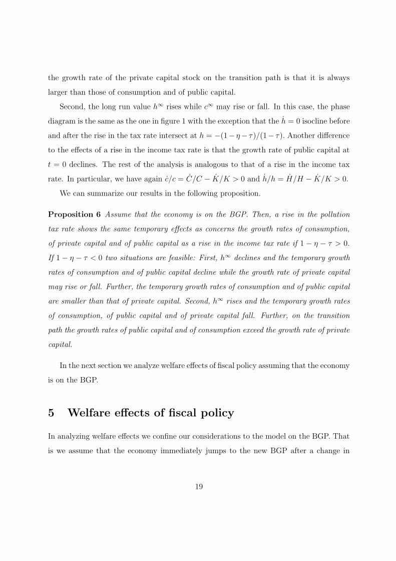
Next, we analyze the effects of a rise in the pollution tax rate τp. To do so we proceed

analogously to the case of the income tax rate. Doing the analysis it turns out that we

have to distinguish between two cases. If 1 − η − τ > 0 the results are equivalent to

those we derived for an increase in the income tax rate.9 If 1 − η − τ < 0 two different

scenarios are possible.10,11 First, the long run values h∞ and c∞ decline. Analogously to

a rise in the income tax rate the c = 0 isocline turns right with c = ρ for h = 0 remaining

unchanged. Further, the new h = 0 isocline lies above (below) the old h = 0 isocline, i.e.

9A detailed derivation is available on request.10For 1 − η − τ = 0 the analysis is equivalent to that of a rise in the income tax rate with the only

difference that ∂(H(t = 0, τ)/H(t = 0, τ))/∂τ = 0 holds.

11Note that in this case the balanced growth rate declines.

17

the isocline before the increase in τp, for h < (>) − (1 − η − τ)/(1 − τ). Since K and H

are predetermined values, the level of consumption must decrease and jump to the stable

manifold implying ∂c(t = 0, τ)/∂τ < 0 to reach the new steady state (c∞, h∞). Figure 2

shows the phase diagram.

Figure 2 about here

Over time both c and h decline until the new BGP is reached at (c∞, h∞). That is

we get c/c = C/C − K/K < 0 and h/h = H/H − K/K < 0 implying that on the

transition path the growth rates of consumption and of public capital are smaller than

that of private capital for all t ∈ [0,∞). The impact of a rise in τp on the growth rate of

private consumption is obtained from (12) as

∂

∂τ

(

C(t = 0, τp)

C(t = 0, τp)

)

= −h1−αα(1 − τ)ϕ < 0,

where we again use that K and H are predetermined variables implying ∂h(t = 0, τ)/∂τ =

0. This shows that at t = 0 the growth rate of private consumption falls as a result of

the increase in the tax rate τp and then continues to decline gradually as the new BGP

is approached. The impact of a rise in τp on the growth rate of public capital is obtained

from (14) as

∂

∂τ

(

H(t = 0, τ)

H(t = 0, τ)

)

= h−α(1 − η − τ)ϕ < 0, for 1 − η − τ < 0

where we again use that h does not change at t = 0. This result states that the growth

rate of public capital declines and then continues to decline over time as the new BGP

is approached. As with a rise of the income tax rate a higher pollution tax rate implies

an instantaneous increase of the tax revenue. However, if η is relatively large, so that

1 − η − τ < 0, a large part of the additional tax revenue is used for abatement activities

so that the growth rate of public capital declines although the tax revenue rises. The

growth rate of the private capital stock may rise or decline. What we can say as to the

18

the growth rate of the private capital stock on the transition path is that it is always

larger than those of consumption and of public capital.

Second, the long run value h∞ rises while c∞ may rise or fall. In this case, the phase

diagram is the same as the one in figure 1 with the exception that the h = 0 isocline before

and after the rise in the tax rate intersect at h = −(1− η− τ)/(1− τ). Another difference

to the effects of a rise in the income tax rate is that the growth rate of public capital at

t = 0 declines. The rest of the analysis is analogous to that of a rise in the income tax

rate. In particular, we have again c/c = C/C − K/K > 0 and h/h = H/H − K/K > 0.

We can summarize our results in the following proposition.

Proposition 6 Assume that the economy is on the BGP. Then, a rise in the pollution

tax rate shows the same temporary effects as concerns the growth rates of consumption,

of private capital and of public capital as a rise in the income tax rate if 1 − η − τ > 0.

If 1 − η − τ < 0 two situations are feasible: First, h∞ declines and the temporary growth

rates of consumption and of public capital decline while the growth rate of private capital

may rise or fall. Further, the temporary growth rates of consumption and of public capital

are smaller than that of private capital. Second, h∞ rises and the temporary growth rates

of consumption, of public capital and of private capital fall. Further, on the transition

path the growth rates of public capital and of consumption exceed the growth rate of private

capital.

In the next section we analyze welfare effects of fiscal policy assuming that the economy

is on the BGP.

5 Welfare effects of fiscal policy

In analyzing welfare effects we confine our considerations to the model on the BGP. That

is we assume that the economy immediately jumps to the new BGP after a change in

19

fiscal parameters. In particular, we are interested in the question of whether growth and

welfare maximization are identical goals.

To derive the effects of fiscal policy on the BGP arising from increases in tax rates at

t = 0 we first compute (1) on the BGP as

J(·) ≡ arg maxC(t)

∫

∞

0e−ρt(ln C(t) − ln PE(t))dt. (19)

Denoting the balanced growth rate by g, (19) can be rewritten as

J(·) = ρ−1(

ln C0 + β g/ρ + β ln η + ln τp − (1 − β) ln ϕ − (1 − β) ln Kα0 H1−α

0

)

, (20)

with C0 = C(0), K0 = K(0) and H0 = H(0). From (12) and (13) we get

g = α(1 − τ)(1 − τpϕ)h1−α − ρ and C0 = K0

(

(1 − τ)(1 − τpϕ)h1−α0 − g

)

.

Combining these two expressions leads to C0 = K0(ρ + g(1 − α))/α. Inserting C0 in (20)

J can be written as

J(·) = ρ−1 (ln(ρ/α + g (1 − α)/α) + β g/ρ + ln τp + C1) , (21)

with C1 a constant given by C1 = ln K0 + β ln η− (1− β) ln ϕ− (1− β) ln(Kα0 H1−α

0 ). (21)

shows that welfare in our economy positively varies with the growth rate on the BGP, i.e.

the higher the growth rate the higher welfare. Differentiating (21) with respect to τ and

τp yields

∂J

∂τ=

∂ g

∂ τ

(

c01 − α

α · ρ+

β

ρ2

)

,∂J

∂τp

=1

τp ρ+

∂ g

∂ τp

(

c01 − α

α · ρ+

β

ρ2

)

. (22)

With the expressions in (22) we can summarize our results in the following proposition.

Proposition 7 Assume that the economy is in steady state and that there exist inte-

rior growth maximizing values for the income and pollution tax rates. Then, the welfare

maximizing pollution tax rate is larger than the growth maximizing rate and the welfare

maximizing income tax rate is equal to the growth maximizing income tax rate.

20

Proof: The fact that the growth maximizing income tax rate also maximizes welfare

follows immediately from (22). Since the pollution tax rate τp maximizes the balanced

growth we have ∂g/∂τp = 0. But (22) shows that for ∂g/∂τp = 0, ∂J/∂τp > 0 holds.

Thus, the proposition is proved. 2

This proposition states that welfare maximization may be different from growth maxi-

mization. If the government sets the income tax rate it can be assured that the income tax

rate which maximizes economic growth also maximizes welfare if one neglects transition

dynamics. However, if the government chooses the pollution tax rate it has to set the

pollution tax rate higher than that value which maximizes the balanced growth rate in

order to achieve maximum welfare. The reason for this outcome is that the pollution tax

rate exerts a direct positive welfare effect by reducing effective pollution in contrast to

the income tax rate. This is seen form (21) where the expression ln τp appears explicitly

but τ does not.

The same also holds for variation of the parameter ϕ which determines the degree of

pollution as a by-product of aggregate production. If ϕ declines, meaning that production

becomes cleaner, there is always a positive partial and direct welfare effect going along

with that effect. Again, this can be seen from (21) where ln ϕ appears. The overall effect

of a decline in ϕ, i.e. of the introduction of a cleaner technology, consists of this partial

welfare effect and of changes in the balanced growth rate.

6 Conclusion

In this paper we have presented an endogenous growth model with public capital and

pollution. The main novelty of our approach compared to the literature on endogenous

growth and environmental pollution is the assumption that pollution only affects the

utility of the household but not production possibilities directly.

Analyzing our model we derived the effects of fiscal policy on the long run balanced

growth rate. We demonstrated that variations in both the income tax rate and the

21

pollution tax rate may have positive or negative growth effects and we derived conditions

which must be fulfilled so that an increase in these tax rates generates a higher balanced

growth rate. In particular, we could derive growth maximizing values of tax rates without

resorting to numerical simulations.

Further, we studied the effects of a rise in the income and pollution tax rate on

the growth rates of consumption, private capital and of public capital on the transition

path and we have seen that the transition effects of fiscal policy may differ from the

long run effects. Finally, we also demonstrated that growth maximization and welfare

maximization need not be equivalent goals. In particular, it turned out that the welfare

maximizing values of parameters are different from the growth maximizing values if the

parameters have a direct impact on effective pollution and, thus, on utility.

22

E

E'

+-

+-

+ -

+ -

c

h

Figure 1

h

c

E'

+-

+-

E

+ -+ -

Figure 2

References

Arrow, K., Kurz, M. (1970) Public Investment, the Rate of Return, and Optimal Fiscal

Policy. The John Hopkins Press, Baltimore.

Aschauer, D.A. (1989) “Is Public Expenditure Productive?” Journal of Monetary Eco-

nomics, Vol. 23: 177-200.

Barro, R.J. (1990) “Government Spending in a Simple Model of Endogenous Growth.”

Journal of Political Economy 98, S103-S125.

Benhabib, J., R. Perli (1994) “Uniqueness and Indeterminacy: On the Dynamics of En-

dogenous Growth.” Journal of Economic Theory 63, 113-142.

Benhabib, J., R. Perli, and D. Xie (1994) “Monopolistic Competition, Indeterminacy

and Growth.” Ricerche Economiche 48, 279-298.

Blanchard, O., and S. Fischer (1989) “Lectures on Macroeconomics.” Cambridge, MA:

The MIT-Press.

Bovenberg, L.A., and S. Smulders (1995) “Environmental Quality and

Pollution-Augmenting Technological Change in a Two-Sector Endogenous Growth

Model.” Journal of Public Economics 57, 369-391.

Byrne, M. (1997) “Is Growth a Dirty Word? Pollution, Abatement and Endogenous

Growth.” Journal of Development Economics 54, 261-284.

Ewijk, C. van, and T. van de Klundert (1993) “Endogenous Technology, Budgetary

Regimes and Public Policy.” In Verbon, Harrie A.A. and van Winden Frans A.A.M.

(eds.), The Political Economy of Government Debt. Amsterdam: North-Holland.

Forster, B.A. (1973) “Optimal Capital Accumulation in a Polluted Environment.” South-

ern Economic Journal 39, 544-547.

23

Futagami, K., Y. Morita, and A. Shibata (1993) “Dynamic Analysis of an Endogenous

Growth Model with Public Capital.” Scandinavian Journal of Economics 95, 607-

625.

Gradus, R., and S. Smulders (1993) “The Trade-off Between Environmental care and

Long-Term Growth - Pollution in Three Prototype Growth Models.” Journal of Eco-

nomics 58, 25-51.

Gruver, G. (1976) “Optimal Investment and Pollution Control in a Neoclassical Growth

Context.” Journal of Environmental Economics and Management 5, 165-177.

Hettich, F. (2000) Economic Growth and Environmental Policy. Edward Elgar, Chel-

tenham, UK.

Lighthart, J.E., and F. van der Ploeg (1994) “Pollution, the Cost of Public Funds and

Endogenous Growth.” Economics Letters 46, 339-49.

Lucas, R.E. (1990) “Supply-Side Economics: An Analytical Review.” Oxford Economic

Papers 42, 293-316.

Luptacik, M., and U. Schubert (1982) “Optimal Economic Growth and the Environment,

Economic Theory of Natural Resources.” Vienna: Physica.

Seierstad, A., and K. Sydsaeter (1987) Optimal Control with Economic Applications.

Amsterdam: North-Holland.

Smulders, S. (1995) “Entropy, Environment, and Endogenous Growth.” International Tax

and Public Finance 2, 319-340.

Smulders, S., Gradus S. (1996) “Pollution abatement and long-term growth.” European

Journal of Political Economy 12, 505-532.

24

Sturm, J.E., Kuper, G.H., de Haan, J. (1998) “Modelling Government Investment and

Economic Growth on a Macro Level.” in S. Brakman, H. van Ees and S.K. Kuipers

(eds.), Market Behaviour and Macroeconomic Modelling, pp. 359-406, Mac Mil-

lan/St. Martin’s Press, London.

25