Albayrak1 and U. Lemmin

Secondary Currents and Corresponding SurfaceVelocity Patterns in a Turbulent Open-Channel

Flow over a Rough BedI. Albayrak1 and U. Lemmin2

Abstract: River and open-channel flows present complex three-dimensional (3D) structures in the water column and on the surface as aresult of the existence of secondary currents driven by either centrifugal force or turbulence. This paper experimentally investigates secondarycurrents in a straight, turbulent, rough-bed open-channel flow; the effect of different channel width to flow depth ratios (12.25, 15, and 20) onsecondary currents; and surface boils associated with secondary currents at moderate Reynolds numbers. Nearly instantaneous profiles ofthree components of flow velocity and turbulence characteristics in the water column were measured by using an acoustic Doppler velocityprofiler (ADVP). Simultaneously, large-scale particle image velocimetry was used to measure the water surface velocities and turbulencestructures. Mean velocity patterns in the water undulate across the channel, indicating the presence of secondary currents in the long-termaverage flow structure. Secondary currents affect the distribution of bed shear stress, Reynolds stress, and turbulence intensities across thechannel. The aspect ratio determines the number of secondary cells in the water column. A mean multiband undulating surface velocitypattern in the transverse direction correlates with the secondary cell distribution in the water column below. The instantaneous position of theupwelling and downwelling regions on the surface may deviate from their long-term mean position, indicating a meandering of the surfacepattern. Vortex structures are detected from instantaneous surface velocity maps, and vortex boil lines are identified. Boil vortices mainlyoccur in upwelling areas with high vorticity. The simultaneous detailed velocity measurements in the water column and on the free surfacehave shown a good agreement between the secondary cell patterns obtained by the two methods. DOI: 10.1061/(ASCE)HY.1943-7900.0000438. © 2011 American Society of Civil Engineers.

CE Database subject headings: Open channel flow; Reynolds stress; Velocity; River beds.

Author keywords: Turbulent open-channel flow; Secondary currents; Reynolds stress; ADVP; Large-scale PIV.

Introduction

River and open-channel flows are free-surface, boundary-layerflows that may contain three-dimensional (3D) large-scale turbu-lent current structures. Different processes occurring at the sametime can generate these structures. Long, straight river or channelsections are characterized by a complex distribution of bed shearstress. These bed shear stress patterns result from secondary cur-rents that are driven by the anisotropy of turbulence (Einsteinand Li 1958). These secondary currents are large-scale streamwisevortical structures that form counterrotating cells across the section.They are called secondary currents of Prandtl’s second kind, andthey play an important role in flow dynamics (Nezu and Nakagawa1993). Between the cells, zones of alternating upwelling anddownwelling motion are created that extend over the whole water

column. Secondary current cells generate an undulating bottomshear stress distribution in the transverse direction. They affectthe whole depth-flow field and the free-surface flow pattern.Related to upwelling and downwelling zones, transverse currentzones of alternating direction and spiral eddies are generated onthe free surface. The resulting flow patterns contribute to sedimenttransport near the bed, change bed and channel forms, and maysignificantly influence the exchange of gas, heat, momentum, andself-aeration at the free surface (Nezu and Nakagawa 1993). In thepast, secondary currents were investigated by measurements carriedout either in the water column or on the water surface.

From measurements in the water column, Kinoshita (1967)showed that secondary current cells scale with water depth and thatlateral spacing between upwelling and downwelling is slightly lessthan l ¼ 2h, where h is the water depth. Tominaga et al. (1989)indicated that secondary currents affect the primary mean flow, thusproducing 3D flow structures. Nezu and Nakagawa (1993) con-cluded that 3D turbulent structures associated with these currentsare almost universal, independent of the Reynolds number. Studiesin wide, open channels relate the origin of secondary current pat-terns to the nonhomogeneity of bed roughness produced by longi-tudinal ridges and troughs on the bed to longitudinal strips of roughand smooth beds or indicate that these bed patterns are reinforcedby preexisting secondary currents (Nezu and Nakagawa 1993).These authors also suggest that preexisting secondary currentsmay be generated by the corner flow between the vertical sidewalland the horizontal bed because of turbulence anisotropy producedat the corner. The secondary current cell in the corner is oftencomposed of an upper and a lower cell (Tominaga et al. 1989).

1Laboratory of Hydraulics, Hydrology and Glaciology (VAW), SwissFederal Institute of Technology (ETH) Zürich, VAW E 35, Gloriastrasse37/39, 8092 Zürich, Switzerland; formerly, School of Engineering, FraserNoble Building, Univ. of Aberdeen, AB24 3UE Aberdeen, UK (corre-sponding author). E-mail: [email protected]

2Laboratory of Environmental Hydraulics (LHE), Ecole PolytechniqueFédérale de Lausanne (EPFL), Switzerland. E-mail: [email protected]

Note. This manuscript was submitted on December 15, 2009; approvedon April 11, 2011; published online on April 13, 2011. Discussion periodopen until April 1, 2012; separate discussions must be submitted for indi-vidual papers. This paper is part of the Journal of Hydraulic Engineering,Vol. 137, No. 11, November 1, 2011. ©ASCE, ISSN 0733-9429/2011/11-1318–1334/$25.00.

1318 / JOURNAL OF HYDRAULIC ENGINEERING © ASCE / NOVEMBER 2011

http://dx.doi.org/10.1061/(ASCE)HY.1943-7900.0000438




In a wide, open channel, Nezu and Rodi (1985) found that the uppercorner cell is enhanced by the damping of the vertical turbulentfluctuations at the water surface compared to the lower one andthat it may extend 2–3h from the sidewall. They also observed thatsecondary currents are generally nonexistent in the center of a fullydeveloped open-channel flow with a width/depth aspect ratio of6 or more. Nezu and Nakagawa (1993) indicated that secondarycurrents are more stable over rough beds than over smooth beds.

Wang and Cheng (2006) investigated experimentally and ana-lytically the time-mean characteristics of cellular secondary flowsgenerated by artificial rigid longitudinal bed forms; they proposedan empirical relationship between the maximum vertical velocityand bed configuration. Rodriguez and Garcia (2008) presentedtime-averaged velocity and turbulence results for the lower partof the water column in medium wide (B=h ¼ 6:3 and 8.5) open-channel flow over a rough bed and reported lateral undulationsof bed shear stress, cores of higher streamwise velocity, andtime-averaged velocity vector and vorticity patterns, from whichthey inferred the whole depth structure of secondary currents. Theysuggested that the interaction between the rough bed and smoothsidewall has a significant impact on secondary current patterns andthe bed shear stress distribution. A strong near-surface vortex at thesidewall is proposed as the main mechanism responsible for thisdistribution.

A number of studies (Komori et al. 1989; Kumar et al. 1998;Tamburrino and Gulliver 1999, 2007) have documented thefree-surface flow field in open-channel flow. Kumar et al. (1998)presented an extensive investigation of free-surface turbulence inshallow smooth-bed, open-channel flow by using high-definitionparticle image velocimetry (PIV) measurement techniques on thesurface. They classified the persistent structures of the free surfaceas upwellings, downdrafts, and spiral eddies. It was shown that atlow Reynolds numbers, upwelling zones were related to burstsoriginating in the sheared region of the water column near the chan-nel bottom, and surface eddies were generated at the edges of theseupwelling zones. These experiments were in good agreement withdirect numerical simulation results from Pan and Banerjee (1995).Tamburrino and Gulliver (1999) worked in a flume with a smoothbottom. They determined that the mean surface velocity pattern iscomposed of alternating surface vortex streets and zones of lowervorticity and higher longitudinal velocity which they called streaks.They suggest that vortex streets occur over upwelling areasand streaks occur over downwelling areas in the water columnbelow. Secondary current patterns shifted in time in the trans-verse direction. Tamburrino and Gulliver (2007) confirmed theseobservations.

Surface boils can be thought of as being formed by the largestreamwise vortices that create upwelling and downwelling regionsat the water surface. Nezu and Nakagawa (1993) suggested threedifferent mechanisms for the generation of surface boils. Their boilsof the second kind are associated with cellular secondary currentsand are seen in wide, straight rivers. They point out that fairly stableboil lines form at the surface between two neighboring secondarycurrent cells. Boils and eddies with a vertical axis are detectedin upwelling zones. Moog and Jirka (1999) studied the effect ofsurface boils on air–gas exchange in detail. They concluded thatin turbulent flows, surface boils contribute to river reaeration andaffect water quality and corresponding management concepts.

The primary goal of this study is to experimentally investigatedetails and driving mechanisms of the structure of secondary cur-rents and the effect of the ratio of channel width to flow depth ofsecondary currents in turbulent open-channel flow over a roughmobile but not moving bed. In previous studies, measurementswere either made in the water column or on the free surface.

In both cases, secondary current patterns were observed. However,no connection between the two approaches was made. In this study,measurements will be simultaneously carried out in the whole watercolumn and on the free surface. This allows an understandingof the structure of secondary currents, quantifies their contributionto transport and mixing throughout the water column, and links it tothe flow field on the free surface. We also examine free-surfaceturbulence structures, such as surface vortices that may be associ-ated with secondary currents and the interaction between the waterflow field and the free-surface flow field.

The first part of this paper describes the experimental setup,procedure, and instrumentation. In the second part, profiles ofthe mean and the instantaneous velocities, turbulence intensities,Reynolds shear stress and bed shear stress across the channel,obtained with an acoustic Doppler velocity profiler (ADVP) areanalyzed for the presence of secondary currents. Thereafter, themean velocity profiles across the water surface obtained with large-scale particle image velocimetry (LSPIV) are examined with re-spect to secondary currents and surface boils and related to themeasurements in the water column.

Background

River and open-channel flows that present complex 3D turbulenceand large-scale structures cannot be represented as two-dimensional (2D) flows. Thus, turbulence models for 2D flows maynot give proper results for 3D flows. Identifying the type of sec-ondary current is essential to understand 3D turbulent flow struc-tures, as secondary currents play an important role in the transversetransfer of momentum, energy, heat, and mass in an open channel.

By using the Reynolds decomposition for the streamwise, thetransverse, and the vertical direction, respectively, the mean veloc-ity components U, W , and V are subtracted from the instantaneousvelocities u, w, and v to obtain the fluctuating components u0, w0,and v0: u0 ¼ u� U, w0 ¼ w�W , and v0 ¼ v� V .

The governing equations for the 3D flow field are the continuityequation and the Reynolds-averaged Navier–Stokes (RANS) equa-tions. In the present case, the flow is uniform and, thus, ∂=∂x ¼ 0in straight open channels. Nezu and Nakagawa (1993) have shownthat one can derive the following equation from them:

V∂Ωdy

þW∂Ω∂z|fflfflfflfflfflfflfflfflfflffl{zfflfflfflfflfflfflfflfflfflffl}

A¼

∂2

∂y∂z ð�v02 � �w02Þ|fflfflfflfflfflfflfflfflfflfflfflffl{zfflfflfflfflfflfflfflfflfflfflfflffl}B

þ

� ∂2

∂z2 �∂2

∂y2�v0w0

|fflfflfflfflfflfflfflfflfflfflfflfflffl{zfflfflfflfflfflfflfflfflfflfflfflfflffl}C

þϑ∇2Ω|fflffl{zfflffl}Dð1Þ

with streamwise vorticity Ω defined as

Ω≡ ∂W∂y � ∂V

∂z ð2Þ

Einstein and Li (1958) proposed to use the vorticity equation[Eq. (2)] to study mechanisms to produce secondary current mo-tion. In Eq. (1), which does not contain the streamwise velocity Uor its fluctuating component u0, the advection of vorticity is indi-cated by term A. The generation of secondary currents is enhancedby the production term B and is suppressed by the Reynolds stressterm C. Terms B and C only contain turbulent velocity componentsin the transverse plane. Nezu and Nakagawa (1984, 1993) andDemuren and Rodi (1984) showed that terms A and D are smallcompared with terms B and C, which have opposite signs. There-fore, secondary currents are driven by the difference between theB and C terms, as discussed by Einstein and Li (1958). Anisotropybetween v0 and w0 generates secondary currents and, in turn, the

JOURNAL OF HYDRAULIC ENGINEERING © ASCE / NOVEMBER 2011 / 1319

secondary current gradient affects the Reynolds stress v0w0. Thedegree of anisotropy between v0 and w0, and thus the secondarycurrents, are influenced by boundary conditions, in particular boun-dary roughness. In turn, the secondary currents affect the transversedistribution of primary flow U, and its distortion changes the bot-tom shear stress τb, which undulates in the transverse direction. Thefeedback between these processes results in a transverse distribu-tion of the Reynolds shear stress u0v0 profile, which is higher thanthe values expected for 2D flows in upwelling regions and lowerthan those in downwelling regions.

Ikeda (1981) assumed a sinusoidal transverse undulation of thebottom shear stress τb. On the basis of terms B and C in Eq. (1) andassuming a linear vertical distribution of the Reynolds stress u0v0but ignoring free-surface and sidewall effects, Ikeda predicted anidealized cellular pattern for secondary currents that arises fromthe anisotropy of turbulence and scales with the water depth.

From observations on the free surface, Tamburrino and Gulliver(1999) found that the large streamwise vortices scale with flowdepth and create upwelling and downwelling motions that they sug-gest relate to secondary currents. The number of secondary upwell-ing and downwelling zones in a channel cross section was given bythe following equations (Tamburrino and Gulliver 1999):

downwelling regions ¼ even integers close to

�AR

2� 3

�ð3Þ

upwelling regions ¼ odd integers close to

�AR

2� 3

�þ 1 ð4Þ

where AR = aspect ratio (B=h).

Experimental Setup and Procedure

All the experiments were carried out in a B ¼ 2:45 m-wide, 27-mlong, 75-cm deep open channel. The bed consisted of mixed gravel,with sizes between 10 mm and 20 mm. The mean gravel size wasd50 ¼ 15 mm. Measurements were carried out in the area 15 m to18 m from the entrance, where the flow field is fully developed. Thedischarge was below the threshold for bed particle motion. Bedslope was zero. As a result of the zero bed slope, the flow is ina state that Yaglom (1979) called moving equilibrium. In this state,water depth and shear velocity vary slowly in the streamwisedirection, and the variation in that direction can be ignored. Theuncertainties in discharge Q, water depth h, and discharge velocityU estimates given in Table 1 were less than 5%.

Three experiments at medium Reynolds number and at differentwidth-to-depth (B=h) ratios were conducted (Table 1). By using theADVP developed at the Ecole Polytechnique Fédérale de Lausanne(EPFL; Rolland and Lemmin 1997; Fig. 1), data were collected fora time t of at least 3 min at each location. This results in a dimen-sionless measurement time, T ¼ tU=h, of the order O(500). As rec-ommended by Nezu and Nakagawa (1993), this is sufficiently longto eliminate the low-frequency fluctuations because measurementsextend over more than 100 bursting events with typical periods ofτ ¼ 1:5–3 s. Because secondary currents are known to scale withwater depth, spanwise spacing of velocity profiles of approximately

20% of the water depth can sufficiently resolve secondary currents.Thus, for each experiment, densely spaced (one profile every2.5 cm between B=h ¼ 2 and 4 from the sidewall, then every 5 cm)ADVP measurements were carried out in a cross section of theflume. For each run, the ADVP was first optimized for the particu-lar conditions (bottom roughness and water depth). ADVP mea-surements were made from above the water surface (Hurther andLemmin 2001). Because the upper 10% of the water column wasslightly disturbed by this installation, it was omitted from thesubsequent analysis. From the data, the authors calculated profilesof the mean values of the three velocity components, the velocityvariance, and the shear stress on the basis of the Reynolds stressprofiles. These were analyzed with respect to the structure ofsecondary currents.

Bottom shear stress was determined with a sensor based on thehot-film principle. The sensor has constant sensitivity in variabletemperature flow (Shen et al. 1998). The film elements weremounted flush on a roughness element (Fig. 2) and were calibratedin situ. Roughness elements on a 10 × 10 cm square around thesensor were glued in place. Therefore, even when the sensorwas moved to a new transverse position, the local flow field aroundthe sensor was not affected by changes in bottom roughness. Thevoltage required to maintain a constant temperature of the thermalelement is related to the wall shear stress

τ b ¼ μ�∂U∂z

��z¼0

ð5Þ

in the form

τ1=2b ¼ AE2 þ B ð6Þwhere τ b = wall shear stress, A and B = constants that have to befound by calibrating the hot-film probe, and E = voltage required tomaintain constant temperature. An in situ calibration as describedin Albayrak et al. (2008) was carried out over a wide range of flowconditions to transform the measured voltage change caused byheat loss by the element into bed shear velocity. From these cali-brations, the error in shear stress on the rough wall was evaluated tobe �5% (Albayrak et al. 2008). By using Eq. (6), the mean bottomshear stress was determined over 3 min at several transverse posi-tions on the same lateral axis of the channel where the ADVP datawere collected at the same time.

For surface-flow visualization, the writers developed a LSPIVsystem (Fig. 3) and used it to measure and visualize 2D water sur-face velocities. The system combines the following componentsand operations: a digital charged-coupled device (CCD) camera,surface illumination, seeding the flow with small light-reflectivewhite particles by using an in-house developed spreading machine,recording short time exposure images of a limited area of the watersurface with a CCD digital camera, processing the recorded videodata and postprocessing PIV data. A monochrome 1.3 megapixel(1; 280 × 1; 024) CMOS SUMIX-150M model camera with a USB2.0 interface was used to cover the surface for one-half of the chan-nel width. Several halogen lights were placed to obtain homo-geneous surface illumination [Fig. 3(a)]. Floating cylindrical(diameter ¼ 1:5 to 2 mm) polypropylene particles were used astracers and coated with paint to minimize agglomeration effects.

Table 1. Hydraulic Parameters for the Experiments

Exp. Qm3=s h cm Um=s Umax m=s u� cm=s Reh Frh B=h d50

S1 0.185 19.5 0.39 0.54 2.83 76.9 103 0.2856 12.25 1.5

S2 0.168 16 0.43 0.60 3.22 68.5 103 0.3432 15 1.5

S3 0.10 12 0.36 0.51 2.65 43.5 103 0.3318 20 1.5


To provide a homogeneous distribution of the particles on the watersurface, a particle-spreading machine was placed upstream of themeasurement field. The bed was painted black for better contrast.The LSPIV software consists of PIV and image processing soft-ware. The PIV software was adapted to our specific conditions re-lated to vortex dynamics. To cover large surface areas, a wide-angleoptic lens was used. A camera calibration toolbox was developedand added to the main PIV software to correct the distorted imagesobtained with this lens. The PIV algorithm is based on a standardcross correlation between two consecutive images by using fastfourier transform (FFT) (Raffel et al. 1998). Because of the highdynamic range of the velocities, adaptive multipass processingwas used, starting with a large interrogation window and by usingthe calculated velocity as a reference for the next smaller interrog-ation window. To remove error vectors, a MATLAB-based, signal-to-noise ratio filter (SNR) programmed by Sveen (2004) is firstused in the postprocessing of PIV raw data to validate the vector

field. SNR filtration discards all vectors when the ratio of the tallestpeak in the correlation plane to the second tallest one is less than1.3. Kean and Adrian (1992) suggested the threshold value of 1.3.The invalid velocity vectors are replaced by the abbreviation NaN(not a number) in the vector matrix. A global filter is used to elimi-nate the vectors that are different from the rest of the vector field. Ifa vector is significantly larger or smaller than most of the vectors,then it is removed from the data. After global filtering, a localmedian filter is applied to the remaining vectors. A local medianfilter sorts velocities on the basis of the squared difference betweenindividual velocity vectors and the median of the mean of their sur-rounding neighbors. The filter takes individual vectors and com-pares them with their closest neighbors. The median of thevectors can easily be replaced with the mean value. Finally, an in-terpolation of the outliers is applied to local median filtered vectors.The program interpolates NaNs in a vector field by using a linearmethod, and the instantaneous velocity field after filtration and in-terpolation of PIV data is obtained. Details of the PIV and imageprocessing software adapted to our specific conditions related tovortex dynamics can be found in Albayrak (2007, 2008).

From the video files, images recorded for 3 min are processedinto instantaneous velocity vector fields. From instantaneous data,time-mean statistics such as mean and root-mean-square (RMS)values and such quantities as vorticity were computed with shortsubprograms in MATLAB. They were analyzed for mean and in-stantaneous velocity patterns that can be associated with secondarycurrents and for boil vortex dynamics linked to upwelling regions.

Experimental Results

This section first presents velocity fields obtained in the water col-umn with the ADVP, followed by surface velocity fields acquiredwith LSPIV. Emphasis is on the velocity patterns related to secon-dary currents, and the effect of relative water depth on these pat-terns is explored.

Mean Velocity Profiles Related to SecondaryCurrents

Fig. 4 shows an idealized sketch of secondary currents across thechannel, the combination of the contour lines of longitudinal meanvelocity U normalized by Umax, and the longitudinal mean velocityprofile at y=h ¼ 0:5 in a half-section of the channel for experimentS2. The maximum velocity appears at approximately 0:1h belowthe water surface near z=h ¼ 2. No velocity-dip phenomenon inthe upper part of the profile occurred because the aspect ratioB=h ¼ 15 is greater than its critical value ðB=hÞc ≅ 5 ÷ 6 (Nezuand Nakagawa 1993). A periodic variation of the contour linesof the longitudinal mean velocity in the lateral direction appears tobe organized between faster and slower moving zones [Fig. 4(b)].The difference between the maximum and the minimum velocity isapproximately 10%, which corresponds to previous observations.The velocity differences can be related to upwelling and downwel-ling regions in the water column that result from secondarycurrents.

Lower longitudinal velocity zones form at approximately z=h ¼2:6, 4.1, and 6; these correspond to regions of upwelling where thecontour lines bulge towards the free surface. The contour lines aredeflected toward the bed at approximately z=h ¼ 1:75, 3.3, 5.1, and7 and thus form zones of higher longitudinal velocity correspond-ing to regions of downwelling.

The lateral spacing l between the lower longitudinal velocityzones near the free surface varies from 1:5h to 2h in the transverse

Fig. 1. Optimized four-receiver configuration of the ADVP developedat the LHE, EPF Lausanne

Fig. 2. Hot-film probes glued onto bottom roughness elements; probesare 3 × 3 mm


direction. This value agrees well with l ¼ 2h, observed in widerivers (B=h ¼ 100) by Kinoshita (1967).

Fig. 5 presents the contour lines of the mean normalized verticalvelocity V (y, z) and the mean normalized vertical velocity profileat y=h ¼ 0:5. Stationary secondary currents are well developed.In Fig. 5, several pairs of upwelling and downwelling regions canbe clearly seen in the cross section, which correspond to the un-dulation of the longitudinal velocity in Fig. 4. The spacing betweencells is again close to the water depth. Close to the wall, a free-surface vortex and a bottom vortex exist. For large aspect ratios,Nezu and Nakagawa (1993) indicated that the spanwise scale ofthis near-surface vortex increases and reaches approximately 2h.In experiment S2, it reaches to 1:75h. Bottom roughness and asmooth sidewall may affect the length scale of the vortex in thisarea. The region of the free-surface vortex shown in Fig. 5 corre-sponds well with the decelerated region of the mean longitudinalvelocity that extends to z=h ¼ 1:75 in Figs. 4(a) and 4(b). Themaximum value of the secondary currents is nearly equal to 2%of the maximum longitudinal velocity, which is close to the valuegiven by Tominaga et al. (1989) and Tamburrino and Gulliver(1999). The mean transverse velocity at the center of the channelis nearly zero, making this the symmetry line of the cellular pattern.Nezu and Nakagawa (1993) obtained similar but less detailedresults.

Transverse velocities support the concept of secondary flowcells over the whole water depth. In Fig. 5, alternating cells ofopposite orientation are found near the top and bottom in a verticalline, indicating repeated flow convergence and divergence in thetransverse direction. Vertical velocities have alternating maximaof upward and downward jets in the upwelling and downwelling

regions. This pattern supports the secondary cell concept developedfor the longitudinal velocities described previously. From Figs. 4and 5, seven stationary secondary cells can be identified in halfthe cross section of the channel. According to Tamburrino andGulliver (1999), 15 secondary cells should exist for the aspect ratioB=h ¼ 15. The missing secondary cell could be explained by theodd-number aspect ratio and the absence of a cell at the channelcenter.

Turbulence Characteristics and Bottom ShearStress Distribution

Reynolds Shear Stress and Bottom Shear Stress

Fig. 6(a) shows the contour lines of the Reynolds shear stresses�u0v0 normalized by the square of the mean bottom friction velocityu2� for experiment S2. The Reynolds shear stress undulates in thelateral direction. Two studies (Nezu et al. 1993; Nezu 2005) pointedout that further from the bed, Reynolds shear stress is higher inupwelling regions of secondary currents (V > 0), but it becomeslower in downwelling regions (V < 0). The pattern and spacingare similar to those seen in the previous figures, confirming Nezu’sobservations. The lateral variation of bed shear stress, τ b, normal-ized by its average value, �τb, obtained from direct measurementwith the hot-film sensor shows relative minimums and maxima[Fig. 6(b)] where upwelling and downwelling regions are expectedfrom the velocity profiles. Bottom shear stress measured by the hotfilm is high below downwelling regions (V < 0) of secondary cur-rent cells and low below upwelling regions (V > 0). The amplitudeof the undulation in the bed shear stress is close to 0.2–0.3 �τb,

Fig. 3. (a) LSPIV and (b) experimental setup


which agrees well with Nezu et al. (1993). The distribution alsocorrelates with the Reynolds shear stress distribution [Fig. 6(a)].Thus, secondary currents significantly influence bottom shearstress. The undulation of the bottom shear stress and Reynoldsshear stress in the spanwise direction can affect sediment particleresuspension and transport and water quality in rivers. This patternis observed here over a rough bed, without any bed forms. There-fore, bed forms caused by secondary currents that have beenreported (Nezu and Nakagawa 1993) may be formed by secondarycurrents and may stabilize the current pattern. However, they arenot necessary for generating them.

Turbulence Intensities

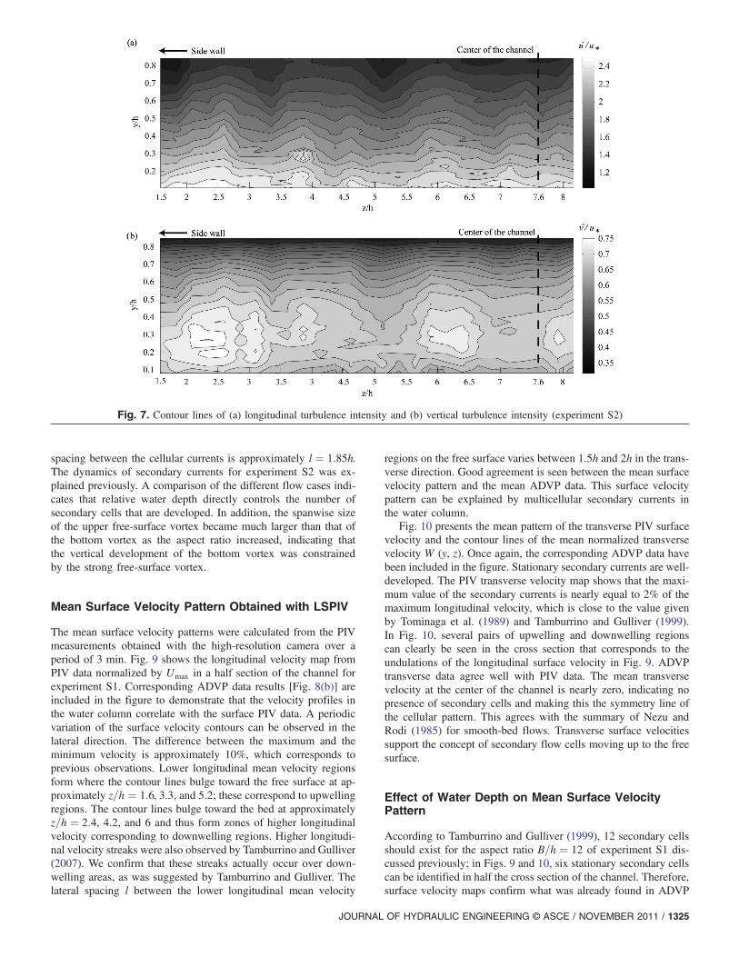
The contour lines of the two components of turbulence intensities,u0 and v0, normalized by u� are given in Figs. 7(a) and 7(b). Theeffect of secondary currents on the turbulence intensities is clearlyseen in these figures.

Turbulence intensities indicate patterns that undulate in the sameway as the mean velocities (Figs. 4 and 5) in the spanwise direction.Away from the bed, turbulence intensity is high in upwellingregions and low in downwelling regions. The contour lines ofvertical turbulence intensity bulge more toward the free surfacethan those of the longitudinal turbulence intensity. This indicatesthat anisotropy of turbulence becomes stronger near the free sur-face, as was pointed out by Nezu et al. (1993) and Hurther et al.(2007). Therefore, secondary currents not only generate a 3Dmean velocity pattern but also affect the turbulence and thusthe mixing in the water column. Laboratory and river data of

Nezu and Nakagawa (1993), which are not as detailed as thepresent data, suggest similar trends.

Effect of Water Depth on the Dynamics ofSecondary Currents

Following Eqs. (3) and (4), the contour lines of the mean longitu-dinal velocity of experiment S1 with an aspect ratio of 12.25, pre-sented in Fig. 8(b), should have four or six downwelling regionsand five or seven upwelling regions. Fig. 8(b) shows six upwellingregions reaching to the free surface and five downwelling regions.Two upwelling regions at z=h ¼ 1:5 are the result of a longitudinalbottom vortex, which is complemented by a surface vortex stretch-ing up to around z=h ¼ 2:4. In experiment S1 with an aspect ratioof 12.25, according to Tamburrino and Gulliver (1999), 12 secon-dary cells should exist for the aspect ratio B=h ¼ 12; from Fig. 8(b),six stationary secondary cells can be identified in half the crosssection of the channel.

Fig. 8(d) shows the contour lines of the mean longitudinal veloc-ity of experiment S3 with an aspect ratio of B=h ¼ 20. Becausethe aspect ratio is 20, according to Tamburrino and Gulliver (1999),20 secondary cells are expected. However, in Fig. 8(d), 22 well-defined secondary cells were found. Relative bottom roughnessmay affect the number of cells, as the aspect ratio of roughnessheight over water depth, which is equal to 12.5%, is higher thanin experiments S1 and S2. In this experiment, the near-surfacevortex in the corner reaches to approximately z=h ¼ 1:8, and the

Fig. 4. Contour lines of (a) the normalized mean longitudinal velocity field and (b) mean longitudinal velocity at y=h ¼ 0:5 (experiment S2)


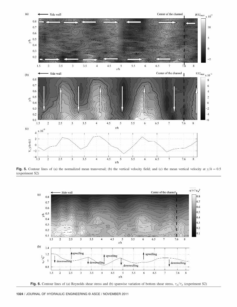
Fig. 5. Contour lines of (a) the normalized mean transversal; (b) the vertical velocity field; and (c) the mean vertical velocity at y=h ¼ 0:5(experiment S2)

Fig. 6. Contour lines of (a) Reynolds shear stress and (b) spanwise variation of bottom shear stress, τb=�τb (experiment S2)


spacing between the cellular currents is approximately l ¼ 1:85h.The dynamics of secondary currents for experiment S2 was ex-plained previously. A comparison of the different flow cases indi-cates that relative water depth directly controls the number ofsecondary cells that are developed. In addition, the spanwise sizeof the upper free-surface vortex became much larger than that ofthe bottom vortex as the aspect ratio increased, indicating thatthe vertical development of the bottom vortex was constrainedby the strong free-surface vortex.

Mean Surface Velocity Pattern Obtained with LSPIV

The mean surface velocity patterns were calculated from the PIVmeasurements obtained with the high-resolution camera over aperiod of 3 min. Fig. 9 shows the longitudinal velocity map fromPIV data normalized by Umax in a half section of the channel forexperiment S1. Corresponding ADVP data results [Fig. 8(b)] areincluded in the figure to demonstrate that the velocity profiles inthe water column correlate with the surface PIV data. A periodicvariation of the surface velocity contours can be observed in thelateral direction. The difference between the maximum and theminimum velocity is approximately 10%, which corresponds toprevious observations. Lower longitudinal mean velocity regionsform where the contour lines bulge toward the free surface at ap-proximately z=h ¼ 1:6, 3.3, and 5.2; these correspond to upwellingregions. The contour lines bulge toward the bed at approximatelyz=h ¼ 2:4, 4.2, and 6 and thus form zones of higher longitudinalvelocity corresponding to downwelling regions. Higher longitudi-nal velocity streaks were also observed by Tamburrino and Gulliver(2007). We confirm that these streaks actually occur over down-welling areas, as was suggested by Tamburrino and Gulliver. Thelateral spacing l between the lower longitudinal mean velocity

regions on the free surface varies between 1.5h and 2h in the trans-verse direction. Good agreement is seen between the mean surfacevelocity pattern and the mean ADVP data. This surface velocitypattern can be explained by multicellular secondary currents inthe water column.

Fig. 10 presents the mean pattern of the transverse PIV surfacevelocity and the contour lines of the mean normalized transversevelocity W (y, z). Once again, the corresponding ADVP data havebeen included in the figure. Stationary secondary currents are well-developed. The PIV transverse velocity map shows that the maxi-mum value of the secondary currents is nearly equal to 2% of themaximum longitudinal velocity, which is close to the value givenby Tominaga et al. (1989) and Tamburrino and Gulliver (1999).In Fig. 10, several pairs of upwelling and downwelling regionscan clearly be seen in the cross section that corresponds to theundulations of the longitudinal surface velocity in Fig. 9. ADVPtransverse data agree well with PIV data. The mean transversevelocity at the center of the channel is nearly zero, indicating nopresence of secondary cells and making this the symmetry line ofthe cellular pattern. This agrees with the summary of Nezu andRodi (1985) for smooth-bed flows. Transverse surface velocitiessupport the concept of secondary flow cells moving up to the freesurface.

Effect of Water Depth on Mean Surface VelocityPattern

According to Tamburrino and Gulliver (1999), 12 secondary cellsshould exist for the aspect ratio B=h ¼ 12 of experiment S1 dis-cussed previously; in Figs. 9 and 10, six stationary secondary cellscan be identified in half the cross section of the channel. Therefore,surface velocity maps confirm what was already found in ADVP

Fig. 7. Contour lines of (a) longitudinal turbulence intensity and (b) vertical turbulence intensity (experiment S2)


measurements in the water column. The contour maps of the meanlongitudinal surface velocity of experiment S2 with an aspect ratioof 15 are shown in Fig. 11. There should be between eight and fivedownwelling regions, and between nine and six upwelling regions.In Fig. 11, four downwelling regions with a higher longitudinalmean velocity are seen in one-half of the channel. Because thecenterline of the channel is the symmetry line, seven downwellingregions can be expected across the channel. The number of upwell-ing regions across the channel is equal to seven. This correspondsto 14 secondary cells for the aspect ratio of 15 in experiment S2.Surface PIV velocity maps agree well with ADVP measurementsfor experiment S2, which are shown in Fig. 4.

Fig. 12 gives the mean longitudinal velocity map for experimentS3. The undulation in the surface velocity map in the spanwisedirection is clearly documented by higher and lower velocity zones.This pattern reveals 11 secondary cells in one-half of the channel.The total number of secondary cells across the channel is 22. Forthe aspect ratio of 20 in experiment S6, 20 cells were expected;however, two additional secondary cells were created in this case.

As indicated previously, our interpretation is that the aspect ratio ofbottom roughness height to water depth is higher than in the otherexperiments, and this affects the dynamics and number of secon-dary cells.

Instantaneous Surface Velocity Pattern

Thus far, we have revealed features of the mean surface flow patternthat were calculated from a superposition of instantaneous velocityvector maps. This pattern is stable. To investigate the instantaneousflow field, individual velocity maps obtained from the PIV data willbe analyzed. The time change will also be analyzed by comparingtwo consecutive maps.

The surface velocity field can be decomposed to detect suchflow structures as vortices, swirling, and upwelling on the watersurface. A vortex is a surface boil, and it is defined as a region ofconcentrated vorticity around which the pattern of streamlines isroughly circular. Vorticity was calculated by using the equationω ¼ dw=dx� du=dz. To determine the size of surface vortices

Fig. 8. Idealized sketch of the secondary currents distribution across a vertical plane for (a) S1 with B=h ¼ 12:25 and (c) S3 with B=h ¼ 20, andcontour lines of the normalized mean longitudinal velocity field for (b) S1 and (d) S3


and the dynamics of upwelling and downwelling regions at the freesurface, streamlines were obtained from the instantaneous flowvelocity field after subtracting the mean velocity field. Fig. 13shows an example of the streamline map with the vorticity field inthe background and the instantaneous velocity vectors of surfacevortices. The mean position of the upwelling and downwellingregions discussed previously are indicated by dashed lines. How-ever, the instantaneous upwelling and downwelling regions do notalways line up with the mean positions, as indicated by the dashedlines. In Fig. 13, one can see a tendency for positive and negativevorticity to align in alternating bands in the flow direction.

Several vortex pairs are seen, mainly near the upwelling regionsat approximately z=h ¼ 3:1 and 5. In the region close to the side-wall, there are smaller vortices. These vortices occur as a result of

the high gradient of the longitudinal velocity with an upwellingregion and zero velocity at the sidewall. Streamlines in this regionbulge toward approximately z=h ¼ 2:2, with positive vorticitycorresponding to a downwelling region.

A pair of spiral eddies labeled G, H, and a vortex, F, at z=h ¼ 3,in Fig. 13(a) create a vortex street in the upwelling region. Detailsof several vortices, as given in Fig. 13(b), indicate that their sizesrange from 0:3h to 1h. The vectors of vortex E are shown in detail.This is a well-formed vortex with high vorticity concentrated at itscenter. Its size is approximately 0:7h and around it, smaller vorticeswith high vorticity are created. Three vortices labeled, A, B, and Cdevelop at z=h ¼ 4:3. A and B are counterrotating vortices withnegative and positive vorticity, respectively, at their center, whereasC is spinning in the same direction as B with positive vorticity.

Fig. 9.Mean pattern of downstream velocity obtained from surface PIV measurements and contour lines of the normalized longitudinal velocity fieldin the water column, obtained from ADVP measurements for experiment S1

Fig. 10.Mean pattern of transversal mean velocity obtained from surface PIV measurements and contour lines of the normalized transversal velocityfield in the water column, obtained from ADVP measurements for experiment S1


Between vortices G and D, a strong downwelling is seen atapproximately z=h ¼ 4, corresponding to the downwelling regiondefined in Figs. 9 and 10. With a negative velocity, between coun-terrotating vortices D and E, a strong upwelling occurs at z=h ¼ 5.There is a downwelling region at the center of the channel withpositive longitudinal velocity. The instantaneous velocity fieldshows the same pattern as the mean velocity map and the ADVPdata. However, in the instantaneous velocity fields, vortices andupwelling regions move and shift slightly in the spanwise direction.

Fig. 14 shows the instantaneous velocity field at time t2 ¼ t1þ0:4 s, where t1 is the time of the map in Fig. 13(a). In Fig. 14,vortex I is well-formed because of an increase in vorticity andgrows in size at the edge of an upwelling region that disappearswith time and space. Vortex F grows and reaches a size equal tothe water depth. Above A and B, a new pair of strong vorticitycenters develop.

Discussion

In this study, we have combined simultaneous hot-film bottomshear stress measurements, 3D nearly instantaneous velocity profilemeasurements taken with an ADVP in the entire water column, andLSPIVon the water surface to reveal patterns of secondary currentsin the long-term average flow structure and the corresponding sur-face flow pattern in three sets of experiments for three differentaspect ratios with moderate Reynolds numbers. This combinationof measurement techniques, which has not been used before in theinvestigation of secondary currents, allows us to deal with all as-pects of the secondary current flow field pattern at the same time.The experiments were carried out in a wider channel, with largerbed grain size and at higher Reynolds numbers than those reportedin the literature (e.g., by Tominaga et al. 1989; Wang and Cheng2006; Rodriguez and Garcia 2008).

Fig. 11. Mean pattern of longitudinal mean velocity obtained from surface PIV measurements for experiment S2

Fig. 12. Mean pattern of longitudinal mean velocity obtained from surface PIV measurements for experiment S3


Cellular Secondary Current Pattern

Possible generation mechanisms for Prandtl’s second kind ofsecondary currents have been proposed by Nezu and Nakagawa(1993). Large-scale turbulent coherent longitudinal eddies occuron smooth, rough, and mobile beds independent of the bed forma-tion. These eddies extend over the entire water column and scalewith water depth. They travel with the bulk flow velocity. On asmooth bed, the temporal mean analysis of flow does not reveala clear pattern of secondary currents, as large-scale longitudinaleddies are unstable and shift instantaneously in the lateral direction.Thus, they can only be detected by an instantaneous time analysis(Nezu 2005). On the other hand, experimental studies have shownthat the large-scale longitudinal eddies are more stable over a roughbed than over a smooth bed (Tominaga et al. 1989; Nezu andNakagawa 1993; Shvidchenko and Pender 2001; Wang and Cheng2006; Rodriguez and Garcia 2008), and thus the temporal meananalysis of these eddies can reveal secondary currents. This wasalso found in the present study, and it was confirmed that secondarycurrents scale with water depth.

Under mobile bed conditions, secondary currents may in-crease the bed nonuniformity and generate ridges and troughs(Shvidchenko and Pender 2001). In the present study, we didnot observe this type of feedback mechanism, as the bed materialwas too coarse to cause bedload or sediment transport at the bottomof the channel. Our study and existing investigations (Tominagaet al. 1989; Rodriguez and Garcia 2008) show a stable distribution

of the secondary currents over a rough bottom with no streamwisebed forms present (e.g., longitudinal ridges and troughs). All ofthese studies have revealed that under these conditions, the mostprobable mechanism for the initiation of multicellular secondarycurrents is the interaction between the rough bed and the smoothsidewall. This was confirmed in our investigation. Anisotropyof turbulence is increased in the corner and generates secondarycurrents. Thus, bed forms are not needed to generate secondary cur-rents. However, they may stabilize the pattern in the long run undermobile bed conditions.

The free-surface vortex in the corner of the channel was thestrongest secondary current cell, and its spanwise size was largerthan that of the bottom vortex in our experiments. The developmentof the bottom vortex was constrained by the strong free-surfacevortex. Similarly, Rodriguez and Garcia (2008) experimentallyfound no evidence of the bottom vortex in their experiments forwidth over depth ratios of 6.3 and 8.5. This suggests that thefree-surface vortex strengthening in the corner is the most likelymechanism for stabilizing the cellular pattern of secondary currentsacross the channel. In addition to the data from the ADVP in thewater column, our LSPIV experiments on the water surface showthat strong free-surface vortices near the sidewall, enhanced bythe upwelling at the smooth wall, initiate and reinforce the cellularpattern of the secondary currents. In our experiments, the trans-verse extent of the surface vortex was between 1.5 and 2h in allexperiments, in agreement with Nezu and Nakagawa (1993) and

Fig. 13. (a) Streamline map with the vorticity field in the background; (b) the instantaneous velocity vectors of surface vortices for S1


McLelland et al. (1999). Rodriguez and Garcia (2008) only found alarger transverse extent of the corner vortex for B=h ¼ 6:3. In thecase of B=h ¼ 8:5, the surface vortex scales with h and is indistin-guishable from the remaining cells. No explanation was given.McLelland et al. (1999), who worked with alternating bands ofsmooth and rough bed, indicate that in order for this vortex patternto develop, a rough band must be closest to the sidewall. Therefore,all observations indicate that the combination of a rough bed and asmooth sidewall lead to the dominance of the surface corner vortex.

In most of our experiments, the strength of the secondary currentcells decays with distance from the sidewall to the center of thechannel. In the center of the channel, cells were either weak or non-existing, making the flow close to 2D. This agrees with Nezu andRodi (1985), who did not observe cells in the center for B=h ¼ 10.Rodriguez and Garcia (2008) measured four and six cells across thefull channel width but did not find a weakening of the cells towardthe center.

The effect of the aspect ratio on the dynamics of secondary cur-rents is significant. The number of secondary current cells changesproportionally with aspect ratio. Tamburrino and Gulliver (1999)proposed this correlation on the basis of free-surface measure-ments. We verified it from measurements within the water columnand on the free surface. By using the information supplied inRodriguez and Garcia (2008) and McLelland et al. (1999), we alsoconfirmed that this relationship holds for their cases. Consideringthat we worked in a very wide channel, and that at the otherextreme, McLeeland et al. (1999) worked in a narrow channel(B=h ¼ 3), the aspect ratio dependence can be considered univer-sal. During our experiments, we also changed the Reynolds numberand the Froude number for a given aspect ratio. This had no effecton the number of cells. Furthermore, our Reynolds number washigher and our grain size was larger than those given in the liter-ature. Therefore, the number of cells is only determined by theaspect ratio.

Mean Velocity Distribution

The transverse distribution of all three velocity components wasmeasured in great detail. Compared to the transverse mean profile,the streamwise velocity in the downwelling regions is slower thanin the upwelling regions. In the wall region, profiles of the meanstreamwise velocity in the upwelling and downwelling regionsdiffer by up to 25%. In the outer layer, the deviation reaches ap-proximately 5%. In general, the difference between upwelling anddownwelling regions is approximately 10%. Rodriguez and Garcia(2008) report a difference of the same order of magnitude for thestreamwise mean velocity.

The maximum mean normalized transverse velocity is ap-proximately 1.5% of the streamwise mean velocity. The strengthof the secondary currents decreases in the spanwise directionand becomes weak at the center of the channel, making this thesymmetry line of the cellular pattern. Nezu and Nakagawa(1993) obtained similar results. However, Tamburrino and Gulliver(1999), in their surface velocity measurements, did not find such adecrease.

By combining streamwise, transverse, and vertical meanvelocity patterns as discussed previously, a synchronized meanvelocity pattern is observed in the whole water and results in aspiraling flow structure, as suggested by Imamoto and Ishigaki(1986).

LSPIV measurements confirmed the observation by Tamburrinoand Gulliver (2007) that higher streamwise surface velocities oc-cur over downwelling regions. We also found slower mean longi-tudinal velocities over upwelling areas. The mean position of theupwelling and downwelling regions in the streamwise surfacevelocity pattern matches those found in the water column. Further-more, the distribution of the mean transverse surface velocitiesagain agrees with the secondary cell pattern. This confirms thatthe surface velocity pattern is an integral part of the secondarycurrent dynamics. Both streamwise and transverse mean surface

Fig. 14. The streamline map with the vorticity field in the background for t2 ¼ t1 þ 0:4 s for S1; t1 is shown in Fig. 13


velocities progressively increase toward the downwelling regions,thus verifying the spiraling flow path of secondary cells proposedby Imamoto and Ishigaki (1986; see also Nezu and Nakagawa1993).

Turbulence

Bottom shear stress obtained from hot-film measurements showedundulations in the spanwise direction. The bottom shear stresshas a high value in the sidewall zone because of the existenceof the corner vortex, which is in agreement with Nezu andNakagawa (1993). Compared to a transverse mean value, strongerbottom shear stress was found in downwelling regions, andweaker bottom shear stress was found in neighboring upwellingregions. The amplitude of the undulation in the bed shear stressis close to 0.2–0.3 τ b, which agrees well with Nezu et al.(1993). Rodriguez and Garcia (2008) reported undulations ofthe same order by using shear velocity values obtained from thelaw of the wall.

A corresponding pattern is revealed for Reynolds stress andturbulence intensity distributions in the water column. Thus, thebottom shear stress distribution is directly affected by the existenceof secondary currents and vice versa. Turbulence structures have3D patterns that undulate in the spanwise direction in the sameway as the mean longitudinal velocity.

In the wall region, streamwise turbulence intensities in down-welling regions are up to 10% greater than in upwelling regions,whereas in the outer region, upwelling enhances turbulence up to10% with respect to downwelling. Close to the free surface, theeffect of upwelling on the streamwise turbulence intensity de-creases to 2% as a result of the free-surface damping effect onturbulence.

Vertical turbulence intensity behaves in the same manner as thestreamwise turbulence intensity. The effect of downwelling on thevertical turbulence intensity is less than that on the longitudinalturbulence intensity. In the wall region, downwelling increasesthe vertical turbulence by up to approximately 6% compared toupwelling, and in the outer region, upwelling enhances the verticalturbulence up to 10% with respect to downwelling.

In downwelling regions, high-momentum fluid is transportedtoward the bed, resulting in an increase of shear stress. In upwellingregions, the opposite occurs. Therefore, anisotropy of turbulencebecomes stronger near the free surface, as was pointed out by Nezuet al. (1993) and Hurther et al. (2007). The results agree well withthose found in the laboratory and river data presented in Nezu andNakagawa (1993). Shvidchenko and Pender (2001) speculated thatthe longitudinal troughs they observed under mobile bed conditionsmay be formed by shear stress modulation caused by nearly sta-tionary secondary currents.

In 3D open-channel flow, because of secondary currents, theReynolds shear stress �u0v0 deviates from the universal lineardistribution found in 2D open-channel flow. Fig. 15 presents thedistribution of Reynolds stress �u0v0 normalized by U2

max atdownwelling and upwelling regions. Fig. 15 also gives the resultsof the experiment that Nezu and Nakagawa (1984) conducted inairflow by using hot-wire measurements. Artificial ridge elementswere used in the air measurements. The spanwise spacing chosenfor the ridges was l ¼ 2h. The flow has upwelling characteristicsover ridges and downwelling characteristics over troughs. Free-surface effects occur for y=h > 0:6. Therefore, air and water flowsare not similar in this region.

Below y=h ¼ 0:6, the present Reynolds stress results have asimilar tendency to those found in Nezu and Nakagawa (1984).As a result of secondary currents, the Reynolds shear stress�u0v0 deviates from the universal linear distribution in both

experiments. In the downwelling region (corresponding to overtroughs in Nezu and Nakagawa 1984), the deviation is negativeand a concave distribution is formed. In the upwelling region (cor-responding to over ridges), the deviation is positive and a convexdistribution is formed. In the wall region, however, the Reynoldsstress in the upwelling region is smaller than that in the downwel-ling region. Therefore, the spanwise variation of �u0v0 close to thebottom is consistent with that of the bottom shear stress. The resultsconfirm the 3D turbulence concept and agree with the previous in-vestigations by Nezu and Nakagawa (1984, 1993). Nezu andNakagawa (1993) point out that this profile form can be explainedby the combined effect of secondary currents and transverse shearstress. Unfortunately, we cannot obtain the parameters from ourmeasurements that are needed to compare our results with theirequation. Rodriguez and Garcia (2008) also report a deviation fromthe linear 2D Reynolds stress distribution. However, no profileforms could be established because their measurements were lim-ited to less than 50% of the water depth.

The undulation of the bottom shear stress and Reynolds shearstress in the spanwise direction is an important factor for masstransport and affects sediment particle distribution and water qual-ity in rivers.

Fig. 16 presents the distribution of Reynolds shear stress

�u0v0=u2� at the center of the channel for experiments S1, S4,and S6, with similar Reynolds numbers at three different waterdepths. Also shown are profiles of spatially averaged Reynoldsshear stress for experiment 1 (with kþs = 355), experiment 2 (withkþs = 325) and experiment 3 (with kþs = 515) conducted by Pokrajacet al. (2007). The present result is in a good agreement with thespatially averaged Reynolds shear stress profiles. In all of theexperiments, the Reynolds shear stress profiles are linear abovethe roughness layer, indicating a 2D turbulence flow structure andconfirming that the secondary currents are negligible (Nezu andNakagawa 1993) and that the flow is two-dimensional. In the walllayer, the effect of relative bottom roughness is significant, and theReynolds shear stress is distributed differently.

Fig. 15. Distribution of Reynolds stress �u0v0 at ∇, z=h ¼ 3:3 (down-welling); ◊, z=h ¼ 4:1 (upwelling) for experiment S2; solid lines:experimental results over ridges and over troughs by Nezu andNakagawa (1984)


Surface Boils

LSPIV measurements permit the detection of vortex structuresfrom the instantaneous velocity map on the water surface byusing the Reynolds decomposition technique. Vortices present aconcentration of vorticity and circular streamline patterns. Vortexboils, such as spiral vortices, were found to mainly occur in theupwelling regions where the mean longitudinal velocity is lower.Vortex size ranges from 0.3 h to 1 h and does not appear to exceedwater depth. The latter value is nearly equal to the distance betweenthe upwelling and downwelling regions.

To investigate whether these surface boils are related to struc-tures in the water column, a quadrant analysis of the streamwiseand vertical fluctuating velocity component was carried out inAlbayrak (2007). Nakagawa and Nezu (1977) suggested a condi-tional probability density function approach for four quadrantsrelating streamwise and vertical velocity fluctuations. Events withQuadrant 1 (u0 > 0, w0 > 0); Quadrant 2 (u0 < 0, w0 > 0); Quad-rant 3 (u0 < 0, w0 < 0); and Quadrant 4 (u0 > 0, w0 < 0) orienta-tions are identified, respectively, as outward interaction, ejection,inward interaction, and sweep events. The equations and the detailsof the technique can be found in Nakagawa and Nezu (1977) and in

Nezu and Nakagawa (1993). This concept was applied to thepresent flow (Albayrak 2007). Quadrant 2 and 4 events at locationsz=h ¼ 2:4 and 3.3, corresponding to a downwelling region and anupwelling region, respectively, were analyzed. To determine the ef-fect of secondary currents on the transverse distribution of coherentstructures, results for y=h ¼ 0:08 in the wall region and y=h ¼ 0:8in the outer layer were evaluated, and the ratios of quadrant valuesof the downwelling region to the upwelling region were deter-mined. Comparing ejection events (Quadrant 2) and sweep events(Quadrant 4) at y=h ¼ 0:08 in the wall region, we can see that forall hole sizes H, sweep events dominate over ejection events. Thisagrees with the observation by Grass (1971) that contributions fromsweep events become larger in the vicinity of the bed. However, inaddition to the previously mentioned tendency for hole size H ¼ 0,the contribution of the ejection event to Reynolds stress becomes10% higher in the downwelling region (z=h ¼ 2:4) than in theupwelling region. At hole size H ¼ 10, the ratio has doubled;it further increases for Quadrant 2 until the hole size reaches 15.At y=h ¼ 0:08, a similar tendency was found for sweep events(Quadrant 4). This result indicates that secondary currents affectturbulence production in the wall region and that downwelling con-tributes more than upwelling to turbulence production. The directhot-film bottom shear stress measurements showed similar results,as bottom shear stress is stronger in the downwelling zone than inthe upwelling zone.

At y=h ¼ 0:8 in the outer layer, a different pattern was observed.A comparison between Figs. 17(a) and 17(b) reveals that in theouter layer, ejection events are significantly more dominant thansweep events for all values of H. For small values of H, upwellingzones contribute almost 10% more to the Reynolds stress thandownwelling zones for both quadrants. For Quadrant 2 events, thistendency continues toward high values of H, with the ratio becom-ing smaller but nearly constant. For Quadrant 4 events, the ten-dency is reversed for H > 5, and the contribution of sweepevents in downwelling zones doubles. The results indicate thatstrong sweeps will create downward transport in downwellingzones and that overall, upwelling zones contribute more stronglyto ejection events in the outer layer. This can be related to the sur-face velocity pattern and the surface boil vortices. On the basis ofbursting frequency and surface renewal frequency measurements,Komori et al. (1989) deduced that most of the surface vortices weregenerated by the ejection process. The present results have estab-lished a relationship between coherent structure dynamics and sec-ondary currents in the water column and boil vortices at the freesurface.

Fig. 16. Distribution of Reynolds stress �u0v0=u2� for experiments S1(▪), S2 (♦), and S3; data by Pokrajac et al. (2007) for experiment 1(Δ); 2 (□) and 3 (●); linear distribution (—)

Fig. 17. Fractional contribution of relative covariance u0v0=u0v0 versus threshold level H at relative flow depth y=h ¼ 0:8 at two different laterallocations, z=h ¼ 2:4 and 3.3


Conclusion

Detailed ADVP, LSPIV, and hot-film measurements have beencombined to analyze secondary current dynamics within the watercolumn and at the free surface of an open-channel flow over arough movable but not moving bed. Previous studies documentedsecondary currents either by measurements in the water columnor at the free surface. In this paper, measurements were combinedto determine the link between secondary current patterns in thewater column and at the free surface. The study was carried outin a wider channel, with a higher bed roughness and at higherReynolds numbers than in previous investigations. The resultsshowed good agreement with the few investigations reported inthe literature.

Patterns of secondary currents in the long-term average flowstructure were investigated in three sets of experiments at threedifferent aspect ratios. Large streamwise vortices occur in thechannel cross section and are more stable and stronger close tothe sidewall. These vortices extend over the entire water columnand scale with water depth; and in the long-term mean, their super-position generates secondary current cells with alternating up-welling and downwelling regions between them. Secondarycurrents show a stable distribution over a rough bottom that hadno bed forms. Therefore, bed forms are not needed to generate sec-ondary currents. However, they may stabilize the pattern in thelong run.

The effect of the aspect ratio on the dynamics of secondary cur-rents is significant. The number of secondary current cells changesproportionally with the aspect ratio. Within the range investigatedhere, the number of secondary current cells is not affected bychanges in the Reynolds number or the Froude number for a givenaspect ratio. No well-defined secondary cell was observed in thecenter zone of the channel. The presence of secondary current cellsmay inhibit the development of a boundary layer in equilibriumwith the bed texture, which is assumed in a 2D description of uni-form open-channel flow.

The transverse distribution of all three mean velocity vectorssupports the concept of secondary currents, showing the alternateappearance of upwelling and downwelling regions. The mean ver-tical velocity presents the clearest pattern of the cellular structure.The mean velocity distribution in the water column and the corre-sponding surface velocities confirm the concept of 3D spiralingflow structures scaling with water depth.

Bottom shear stress obtained from hot-film measurementsshowed undulations in the spanwise direction. Stronger bottomshear stresses were found in downwelling regions, and weakerbottom shear stresses were found in neighboring upwelling regions.A corresponding pattern is revealed for Reynolds stress and turbu-lence intensity distribution in the water column. Thus, the bottomshear stress distribution is directly affected by the existence ofsecondary currents and vice versa. Secondary currents changethe distribution of turbulence intensities and Reynolds shear stressin the water column. Upwelling regions show higher turbulenceintensities and Reynolds shear stress above the roughness layer,whereas downwelling regions show lower values. Therefore, sec-ondary currents affect all scales of the flow field. In rivers and openchannels, mass transport related to sediment particle distributionand water quality may be influenced by this spanwise variationof bottom shear stress, which may contribute to the formation ofbed forms in the case of mobile beds.

Surface vortex boil lines near upwelling regions are identifiedwith LSPIV measurements. Vortex structures are detected from theinstantaneous velocity map of the water surface by using theReynolds decomposition technique. The vortices can be related to

ejections in the upwelling region. Vortex size does not exceed waterdepth, and its size ranges from 0.3 h to 1 h, which is nearly equalto the distance between upwelling and downwelling regions. Theinstantaneous position of the upwelling and downwelling regionsmay deviate from the long-term mean position, indicating a mean-dering of the surface pattern.

Our investigations show that secondary currents producespiraling 3D flow structures and contribute to surface renewaland gas transfer. In downwelling regions, the water masses thatare moved across the surface by the transverse surface currentswill be transported downward faster than by turbulence mixing.Dispersion and mixing caused by secondary currents providefor rapid 3D distribution in the entire water column, as all scalesof the velocity field are affected by the presence of secondary cur-rents. From the similarity between open-channel flow and rivers,we can infer that they are important processes in river dynamicsthat affect transport processes between the free surface and thepelagic zone.

Considering that these experiments were carried out in a muchwider channel and at much higher Reynolds numbers than thosereported in the literature and that the results agree with most ofthe findings in the literature, the dynamics and the characteristicsof secondary currents and the corresponding surface velocitiesappear to be universal.

Acknowledgments

The writers are grateful for the financial support that was providedby the Swiss National Science Foundation (grant 200020-100383)for this study. We would like to thank to the anonymous reviewersfor their constructive comments.

References

Albyarak, I. (2007). “Secondary currents and coherent structures, theirdistribution across a cross section and their relation to surface boilsin turbulent gravel-bed open-channel flow.” 32nd Congress of IAHR,John F. Kennedy Student Competition, Venice, Italy.

Albayrak, I. (2008). “An experimental study of coherent structures, secon-dary currents and surface boils and their interrelation in open-channelflow.” Ph.D. thesis, Ecole Polytechnique Fédérale de Lausanne (EPFL),Switzerland.

Albayrak, I., Hopfinger, E., and Lemmin, U. (2008). “Near field flow struc-ture of a confined wall jet on flat and concave rough walls.” J. FluidMech., 606, 27–49.

Demuren, A. O., and Rodi, W. (1984). “Calculation of turbulence drivensecondary motion in non-circular conduits.” J. Fluid Mech., 140,190–222.

Einstein, H. A., and Li, H. (1958). “Secondary currents in straightchannels.” Trans., Am. Geophys. Union, 39, 1085–1088.

Grass, A. J. (1971). “Structural features of turbulent flow over smooth andrough boundaries.” J. Fluid Mech., 50, 233–255.

Hurther, D., and Lemmin, U. (2001). “Discussion of equilibrium near-bedconcentration of suspended sediment by Z. Cao.” J. Hydraul. Eng., 127,430–433.

Hurther, D., Lemmin, U., and Terray, E. A. (2007). “Turbulent transport inthe outer region of rough-wall open-channel flows: the contribution oflarge coherent shear stress structures (LC3S).” J. Fluid Mech., 574,465–493.

Ikeda, S. (1981). “Self-forced straight channels in sandy beds.” J. Hydraul.Div., 107, 389–406.

Imamoto, H., and Ishigaki, T. (1986). “Visualization of longitudinal eddiesin open-channel flow.”Proc., 4th Int. Symp. on Flow Visualization,C. Veret, Paris, 333–337.

Kean, R. D., and Adrian, R. J. (1992). “Theory of cross-correlation analysisof PIV images.” J. Appl. Sci. Res., 49, 191–215.


Kinoshita, R. (1967). “An analysis of the movement of flood waters byaerial photography.” Photographic Surv., 6, 3109–3116.

Komori, S. Y., Murakami, Y., and Ueda, H. (1989). “The relationshipbetween surface-renewal and bursting motions in an open-channelflow.” J. Fluid Mech., 203, 103–123.

Kumar, S., Gupta, R., and Banerjee, S. (1998). “An experimental investi-gation of the characteristics of free-surface turbulence in channel flow.”Phys. Fluids, 10, 437–456.

McLelland, S. J., Ashworth, P. J., Best, J. L., and Livesey, J. R. (1999).“Turbulence and secondary flow over sediment stripes in weaklybimodal bed material.” J. Hydraul. Eng., 125(5), 463–473.

Moog, D. B., and Jirka, G. H. (1999). “Air-water gas transfer in uniformchannel flow.” J. Hydraul. Eng., 125(1), 3–10.

Nakagawa, H., and Nezu, I. (1977). “Prediction of the contribution to theReynolds stress from bursting events in open channel flows.” J. FluidMech., 80, 104–143.

Nezu, I. (2005). “Open-channel flow turbulence and its research prospect inthe 21st century.” J. Hydraul. Eng., 131(4), 229–246.

Nezu, I., and Nakagawa, H. (1984). “Cellular secondary currents in astraight conduit.” J. Hydraul. Eng., 110(2), 173–193.

Nezu, I., and Nakagawa, H. (1993). “Turbulence in open-channel flows.”IAHR monograph series, Balkema, Netherlands.

Nezu, I., and Rodi, W. (1985). “Experimental study on secondary currentsin open channels flow.” Proc., 21st Congress of IAHR, 2, Melbourne,Australia, 19–23.

Nezu, I., Tominaga, A., and Nakagawa, H. (1993). “Field measurementsof secondary currents in straight rivers.” J. Hydraul. Eng., 119(5),598–614.

Pan, Y., and Banerjee, S. (1995). “Numerical investigation of free-surfaceturbulence in open-channel flows.” Phys. Fluids, 7, 1649.

Pokrajac, D., Campbell, L. J., Nikora, V., Manes, C., and McEwan, I.

(2007). “Quadrant analysis of persistent spatial velocity perturbationsover square-bar roughness.” Exp. Fluids. 42, 413–423.

Raffel, M., Willert, C., and Kompenhans, J. (1998). Particle image veloc-imetry, A practical guide, Springer-Verlag, Berlin.

Rodriguez, J. F., and Garcia, M. H. (2008). “Laboratory measurements of3-D flow patterns and turbulence in straight open channel with roughbed.” J. Hydraul. Res., 46, 454–465.

Rolland, T., and Lemmin, U. (1997). “A two-component acoustic velocityprofiler for use in turbulent open-channel flow.” J. Hydraul. Res., 35,545–561.

Shen, C., Song, T., and Lemmin, U. (1998). “Skin friction measurement invariable temperature flow.” IEEE Instrumentation and MeasurementTechnology Conference, Brussels, 523–526.

Shvidchenko, A. B., and Pender, G. (2001). “Macroturbulent structureof open-channel flow over gravel beds.” Water Resour. Res., 37(3),709–719.

Sveen, J. K. (2004). “An introduction to MatPIV v.1.6.1, Eprint no. 2.”Dept. of Mathematics, Univ. of Oslo, Norway.

Tamburrino, A., and Gulliver, J. S. (1999). “Large flow structures in aturbulent open channel flow.” J. Hydraul. Res., 37, 363–380.

Tamburrino, A., and Gulliver, J. S. (2007). “Free-surface visualizationof streamwise vortices in a channel flow.” Water Resour. Res., 43,wi1410.

Tominaga, A., Nezu, I., Ezaki, K., and Nakagawa, H. (1989). “Three-dimensional turbulent structure in straight open-channel flows.”J. Hydraul. Res., 27, 149–173.

Wang, Z. Q., and Cheng, N. S. (2006). “Time-mean structure of secondaryflows in open channel with longitudinal bedforms.” Adv. Water Resour.,29(11), 1634–1649.

Yaglom, A. M. (1979). “Similarity laws for constant-pressure and pressure-gradient turbulent wall flows.” Annu. Rev. Fluid Mech., 11, 505–540.


Copyright of Journal of Hydraulic Engineering is the property of American Society of Civil Engineers and its

content may not be copied or emailed to multiple sites or posted to a listserv without the copyright holder's

express written permission. However, users may print, download, or email articles for individual use.

Documents

Albayrak1 and U. Lemmin