ALASKA DEPARTMENT OF TRANSPORTATION

Parks Highway Load Restriction

Study: Field Data Analysis

Prepared by: Lutfi Raad

Institute of Northern Engineering University of Fairbanks Alaska PO Box 755900 Fairbanks AK 99775

March 1998 Prepared for: Alaska Department of Transportation Statewide Research Office 3132 Channel Drive Juneau, AK 99801-7898 AK-RD-98-07

Alaska D

epartment of T

ransportation & P

ublic Facilities

Research &

Technology T

ransfer

TRANSPORTATION RESEARCH CENTER

Parks Highway Load Restriction Study Field Data Analysis

by

Lutfi Raac

February1998

FINAL REPORT

Report No. INE/TRC 97.11

US. Department of Transportation Federal Highway Administration

UAF RESEARCH CENTER

UNIVERSITY OF ALASKA FAIRBANKS FAIRBANKS, ALASKA

99775-5900

Technical Report Documentation Page

1. Report No.

I N E m C 97.1 1

F

2. Government Accession No. 3. Recipient's Catalog No.

7. Author@) Lutfi Raad, G. Minassian, S . Saboundjian. M. Stone, X. Yuan, and T. Zhang

4. Title and Subtitle

Parks Highway Load Restriction Study Field Data Analysis

8. Performing Organization Report No. INERRC 97.1 1

5. Reporting Date March 1998

6. Performing Organization Code

17. Key Words highway, damage assessment, rutting!, thaw period frozen ground, asphalt fatigue

19. Security Classif. (of this report)

nonclassified nonciassifed

20. Security Classif. (of this page)

18. Distribution Statement

21. No. of Pages 104

22. Price

9. Performing Organization Name and Address

Institute of Northern Engineering University of Alaska Fairbanks Fairbanks, AK 99775-5900

10. Work Unit No. (TRAIS)

11. Contract or Grant No.

12. Sponsoring Agency Name and Address State of Alaska Alaska Dept. of Transportation and Public Facilities En ineering and Operations Standards 3 I f 2 Channel Drive Juneau, Alaska 99801-7898

13. Type of Report and Period Covered. Final, 1995-97

~

14. Sponsoring Agency Code

15. Supplementary Notes Performed in cooperation with the Federal Highway Administration.

16. Abstract

The loss of pavement strength during spring thaw could result in excessive road damage under applied traffic loads. Damage assessment associated with the critical thaw period is essential to evaluate current load restriction policies. The Alaska Department of Transportation and Public Facilities (AKDOT&PF) proposed a plan which will provide an engineering analysis of field conditions with 100% loads on the Parks Highway for 1996. The study was jointly conducted by AKDOTUF, the Alaska Trucking Association (ATA), and the University of Alaska Fairbanks Institute of Northern Engineering Transportation Research Center (TRC). Extensive field data were collected and analyzed in an effort to monitor pavement damage during the spring of 1996 and determine the loss of pavement strength. The field data included:

1.) Truck traffic data using the Chulitna weigh in motion (WIM) station and the scalehouses at Eagle River and Ester. WIM data were obtained for both northbound and southbound traffic from 1993-1996. Scalehouse data were obtained for Spring 1996 for comparison with WIM spring data.

2.) Pavement temperature data (Spring 1996) for seven ground temperature sites representing typical conditions along the Parks Highway.

3.) Profilometer data for pavement roughness and rutting obtained yearly (1993,1995, and 1996) and also monitored over shorter intervals during Spring 1996. In addition, rut-bar measurements at selected points were also monitored during Spring 1996.

Final Report

PARKS HIGHWAY LOAD RESTRICTION STUDY FIELD DATA ANALYSIS

VOLUME 1

Lutfi Raad, Ph.D.

Professor of Civil and Environmental Engineering Director, Transportation Research Center

Institute of Northern Engineering University of Alaska Fairbanks

Fairbanks, Alaska 99775

G. Minassian S . Saboundjian

M. Stone X. Yuan T. Zhang

Research Assistants Transportation Research Center

Institute of Northern Engineering University of Alaska Fairbanks

Fairbanks, Alaska 99775

and

David Bush

Dynatest Consulting Inc. Ojai, California

February 1998

DISCLAIMER

The contents of this report reflect the views of the authors, who are responsible for the

nccuracy of the data presented herein. This document is disseminated through the

Transportation Research Center, Institute of Northern Engineering, University of Alaska

Fairbanks. This research has been funded by the Alaska Department of Transportation

and Public Facilities (AKDOT&PF) and the Federal Highway Administration. The +

contents of this report do not necessarily reflect the views or policies of AKDOT&PF or

any local sponsor. This work does not constitute a standard, specification, or regulation.

11

... 111

ABSTRACT

The loss of pavement strength during spring thaw could result in excessive road damage tindcr applied traffic loads. Damage assessment associated with the critical thaw period is essential to evaluate current load restriction policies. The Alaska Department of 'T'ransportation and Public Facilities (AKDOT&PF) proposed a plan which will provide an engineering analysis of field conditions with 100% loads on the Parks Highway for 1996. The study was jointly conducted by AKDOT&PF, the Alaska Trucking Association (ATA), and the University of Alaska Fairbanks Institute of Northern Engineering Transportation Research Center (TRC). Extensive field data were collected and analyzed in an effort to monitor pavement damage during the spring of 1996 and dctertnine the loss of pavement strength. The field data included:

1 .

2.

3.

4.

Truck traffic data using the Chulitna weigh in motion (WIM) station and the scalehouses at Eagle River and Ester. WIM data were obtained for both northbound and southbound traffic from 1993- 1996. Scalehouse data were obtained for Spring 1996 for comparison with WIM spring data.

Pavement temperature data (Spring 1996) for seven ground temperature sites representing typical conditions along the Parks Highway.

Profilometer data for pavement roughness and rutting obtained yearly (1993,1995, and 1996) and also monitored over shorter intervals during Spring 1996. In addition, rut-bar measurements at selected points were also monitored during Spring 1996.

Falling Weight Deflectometer (FWD) data for both the northbound and southbound lanes for selected sections in lengths of eight 8 km (5 mile) along the Parks Highway. These data were used in backcalculation of pavement layer moduli, fatigue strength of the asphalt concrete surface, and corresponding damage factors resulting from spring-thaw weakening.

Field data were used to analyze the damage effects on the Parks Highways. These included: analysis and comparison of WIM and scalehouse traffic data; determination of overweight axle loads and vehicles; comparison of north- and southbound traffic and its effect on pavement damage; analysis of ground temperature for thaw initiation and propagation; and simulation of the pavement's remaining life, with and without load restrictions, using mechanistic methods. This report presents results of these analyses.

Table of Contents

Page

Disclaimer ....................................................................................................................... 11

Abstract .......................................................................................................................... 111

Table of Contents .......................................................................................................... iv

List of Tables .................................................................................................................. v

..

...

.. List of Figures .............................................................................................................. vn

Acknowledgments .......................................................................................................... xi

1 . INTRODUCTION ....................................................................................................... 1

2 . FIELD DATA COLLECTION AND ANALYSIS ....................................................... 2

3 . TRAFFIC DATA ANALYSIS ..................................................................................... 7

4 . ANALYSIS OF GROUND TEMPERATURE DATA ............................................... 15

5 . ANALYSIS OF FIELD RUTTING AND ROUGHNESS .......................................... 17

6. ANALYSIS OF FWD AND STRUCTURAL CONSIDERATIONS .......................... 27

7 . SUMMARY AND CONCLUSIONS ........................................................................ 33

8 . REFERENCES ............................................................................. : 35 ..........................

Appendix A : Profilometer Rut and IRI Data (Yearly and Seasonal) ........................ Vol . 2

Appendix B : Rut Bar Measurements (Spring 1996) ................................................ Vol . 2

Appendix C : Condition Survey (Visual Observations) ............................................ Vol . 2

Appendix D : Axle Load Distributions (WIM Data) ................................................ Vol . 2

Appendix E : Axle Load Distributions (Scalehouse Data) ........................................ Vol . 2

Appendix F : FWD Data .......................................................................................... Vol . 2

iv

List of Tables

Page

Table 1 . Selected Field Test Sections along the Parks Highway ........................................ 2

Table 2 . A Summary of Maintenance Activities for the Selected Sections ....................... 3

Table 3 . Type and Frequency of Testing and Field Observation Performed ..................... 4

Table 4 . Standard and Maximum Legal Axle Loads ......................................................... 6

Table 5 . Site Location for Monitoring Pavement Location and Corresponding Parks Highway Section .............................................................. 7

‘I’able 6 . Scalehouse (Glenn Highwaymster) and WIM (Chulitna) 1996 Truck Traffic ............................................................................................ 8

Table 7 . Average and Standard Deviation of Axle Groups from Chulitna WIM Station .................................................................................................... 9

Table 8 . Average and Standard Deviation of Axle Groups from Glenn Highway/Ester Scalehouse ................................................................................. 9

Table 9 . Ratio Scalehouse to WIM Average Axle Loads ............................................... 10

Table 10 . Average Axle Load Ratios Used to Adjust WIM Axle Loads ......................... 11

Table 1 1 . Summary of EALNehicle (Class 5-13) with and without Load Restrictions ............................................................................... 12

Table 12 . Percent Overload for Different Axle Groups during Spring-Thaw Period ........................................................................................ 13

Table I 3 . Percent Damage Contribution of Different Axle Groups during Spring-Thaw ........................................................................................ 14

Table 14 . Percent “Spring-Thaw” Damage Resulting from Overload of Axle Groups ............................................................................... 14

Table 15 . Regression Parameters for Thaw Propagation Relationships ........................... 16

Table I6 . Estimated 1996 Dates for Thaw Initiation and Propagation ........................... 16

List of Tables (continued)

Page

Field Sections on the Parks ............................................................................ 18 Table 17 . A Summary of Distress Observed for the Selected

Table 18 . Comparison of Northbound and Southbound Observed Distress ..................... 18

Table 19 . Average Profilometer Rut Data and Standard Deviation ................................. 20

Table 20 . Average IRI Data and Standard Deviation ...................................................... 21

Table 2 1 . Average Rut Bar Data and Standard Deviation Northbound Lane ........................................................................................... 22

Table 22 . Average Rut Bar Data and Standard Deviation Southbound Lane ........................................................................................... 23

Table 23 . Comparison of Northbound and Southbound Rutting and IRI ........................ 25

Table 24 . Regression Coefficients for Incremental Rutting Damage Model .................. 26

'Table 25 . Regression Coefficients for Incremental IRI Damage Model ......................... 26

Table 26 . Pavement Thicknesses for Parks Highway Sections ...................................... 28

Table 27 . Regression Coefficients for Rut vs . EAL Model ............................................. 28

Table 28 . Regression Coefficients for IRI vs . EAL Model ............................................. 29

Table 29 . Estimated Improvement in Remaining Life Resulting from Load Restrictions ................................................................................... 32

Figure

Figure

Figure

List of Figures

Page

Figure 1 . Steering Axle Load Distribution (Winter 1995) .............................................. 37

Figure 2 . Steering Axle Load Distribution (Spring 1995) ............................................... 38

Figure 3 . Steering Axle Load Distribution (Summer 1995) ............................................ 39

Figure 4 . Steering Axle Load Distribution (Fall 1995) ................................................... 40

Figure 5 . Single Axle Load Distribution (Winter 1995) ................................................ 41

Figure 6 . Single Axle Load Distribution (Spring 1995) ................................................. 42

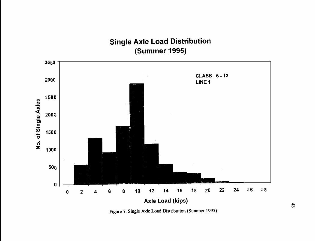
Ia'igure 7 . Single Axle Load Distribution (Summer 1995) ................................................ 43

Figure 8 . Single Axle Load Distribution (Fall 1995) ...................................................... 44

Figure 9 . Tandem Axle Load Distribution (Winter 1995) ............................................... 45

Figure I O . Tandem Axle Load Distribution (Spring 1995) ............................................. 46

Figure 1 1 . Tandem Axle Load Distribution (Summer 1995) .......................................... 47

Figure 12 . Tandem Axle Load Distribution (Fall 1995) ................................................. 48

Figure 1 3 . Average Trucks/Day Monthly Distribution (1995) ........................................ 49

4 . Monthly EAL Distribution (1995) ................................................................. 50

5 . Average EAL/Veh . Monthly Distribution (1995) ......................................... 51

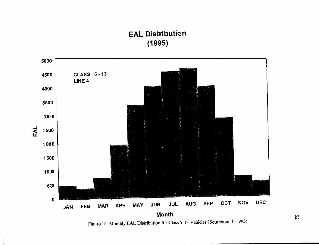
6 . Monthly EAL Distribution for Class 5-13 Vehicles (Southbound -1995) ..................................................................................... 52

(Southbound . 1995) ..................................................................................... 53 ligure 17 . Monthly EAL Distribution for Class 13 Vehicles

Figure 18 . Monthly EAL Distribution for Class 5-13 Vehicles (Northbound . 1995) .................................................................................... 54

Figure 19 . Monthly EAL Distribution for Class 13 Vehicles (Northbound . 1995) ........ ............................................................................ 55

vii

List of Figures (continued)

Page

(Southbound -1996) ...................................................................................... 56 Figure 20 . Monthly EAL Distribution for Class 5-13 Vehicles

Figure 21 . Monthly EAL Distribution for Class 13 Vehicles (Southbound . 1996) ...................................................................................... 57

Figure 22 . Monthly EAL Distribution for Class 5-13 Vehicles (Northbound . 1996) ..................................................................................... 58

Figure 23 . Monthly EAL Distribution for Class 13 Vehicles (Northbound . 1996) ..................................................................................... 59

Figure 24 . Thaw Depth Propagation (Palmer) ................................................................ 60

Figure 25 . Thaw Depth Propagation (Willow) ............................................................... 61

Figure 26 . Thaw Depth Propagation (Chulitna) .............................................................. 62

Figure 27 . Thaw Depth Propagation (East Fork) ........................................................... 63

Figure 28 . Thaw Depth Propagation (Cantwell) ............................................................. 64

Figure 29 . Thaw Depth Propagation (Nenana) ............................................................... 65

Figure 30 . Thaw Depth Propagation (Fox) ..................................................................... 66

Figure 3 1 . Comparison of Yearly and Seasonal IRI ( M P 120 . Northbound) .................. 67

Figure 32 . Comparison of Yearly and Seasonal IRI (Clear . Northbound) ...................... 68

Figure 33 . Comparison of Yearly and Seasonal Rutting (MP 120 . Northbound) ................................................................................ 69

Figure 34 . Comparison of Yearly and Seasonal Rutting (Clear . Northbound) ..................................................................................... 70

Figure 35 . Comparison of Northbound and Southbound IRI and Rutting (Wasilla) ........................................................................................... 71

Figure 36 . Comparison of Northbound and Southbound IRI and Rutting (Big Lake) ........................................................................................ 72

... V l l l

List of Figures (continued)

Page

Rutting (MP 120) .......................................................................................... 73 Figure 37 . Comparison of Northbound and Southbound IRI and

Figure 38 . Comparison of Northbound and Southbound IRI and Rutting (MP 150) ......................................................................................... 74

Figure 39 . Comparison of Northbound and Southbound IRI and Rutting (East Fork) ....................................................................................... 75

Figure 40 . Comparison of Northbound and Southbound IRI and Rutting (Clear) ............................................................................................. 76

Figure 41 . Comparison of Northbound and Southbound IRI and Rutting (Nenana) ........................................................................................... 77

Figure 42 . Comparison of Northbound and Southbound IRI and Kutting (Ester) .............................................................................................. 78

Figure 43 . Rutting Prediction with EAL for Parks Highway Sections ............................. 79

Figure 44 . IRI Prediction with EAL for Parks Highway Sections ................................... 80

Figure 45 . Comparison between Predicted and Measured Rutting .................................. 81

Figure 46 . Comparison between Predicted and Measured IRI ....................................... 82

Figure 47 . Typical Backcalculated Moduli and Damage Factors for Wasilla Section ............................................................................................ 83

Figure 48 . Typical Backcalculated Moduli and Damage Factors for Big Lake Section .......................................................................................... 84

Figure 49 . Typical Backcalculated Moduli and Damage Factors for MP 120 Section ............................................................................................ 85

Figure SO . Typical Backcalculated Moduli and Damage Factors for MP 150 Section ............................................................................................. 86

Figure 5 I . Typical Backcalculated Moduli and Damage Factors for East Fork Section ........................................................................................ 87

ix

List of Figures (continued)

Page

Clear Section ................................................................................................. 88 Figure 52. Typical Backcalculated Moduli and Damage Factors for

Figure 53. Typical Backcalculated Moduli and Damage Factors for Nenana Section ............................................................................................ 89

Figure 54. Typical Backcalculated Moduli and Damage Factors for Ester Section ................................................................................................. 90

Figure 55. Remaining Life Ratio Variation with Damage Factor .................................... 81

Figure 56. Limiting Damage Factor Variation With Thaw Depth Period ........................ 92

Figure 57. Effect of AC Surface Thickness on Damage Consumption Factor (Raad et al. 1997) .......................................................................................... 93

X

ACKNOWLEDGMENTS

This work has been sponsored by the Alaska Department of Transportation and Public

Facilities and the Federal Highway Administration. Additional support was provided by

Alaska Trucking Association. Eric Johnson and Tony Barter of the Alaska Department of

Transportation and Public Facilities provided technical advice and feedback during the

course of the study. This help is greatly appreciated.

xi

1. INTRODUCTION

The loss of pavement strength during spring thaw could result in excessive road damage under applied traffic loads. Damage assessment associated with the critical thaw period is essential to evaluate current load restriction policies. The Alaska Department of Transportation and Public Facilities (AKDOT&PF) has proposed a plan which will provide an engineering analysis of field conditions with 100% loads on the Parks Highway for 1996. The study was jointly conducted by AKDOT&PF, the Alaska Trucking Association (ATA), and the University of Alaska Fairbanks Transportation Research Center (TRC). Extensive field data were collected and analyzed in an effort to monitor pavement damage during the spring of 1996 and determine the loss of pavement strength. The field data included:

1.

2.

3.

4.

Truck traffic data using the Chulitna weigh in motion (WIM) station and the scalehouses at Eagle River and Ester. WIM data were obtained for both northbound and southbound traffic from 1993- 1996. Scalehouse data were obtained for Spring 1996 for comparison with WIM spring data.

Pavement temperature data (Spring 1996) for seven ground temperature sites representing typical conditions along the Parks Highway.

Profdometer data for pavement roughness and rutting obtained yearly (1993,1995, and 1996) and also monitored over shorter intervals during Spring 1996. In addition, rut-bar measurements at selected points were also monitored during Spring 1996.

Falling Weight Deflectometer (FWD) data for both the northbound and southbound lanes of eight 8 km (5 mile) long selected sections along the Parks Highway. These data were used in backcalculation of pavement layer moduli, fatigue strength of the asphalt concrete surface, and corresponding damage factors resulting from spring-thaw weakening.

2

Field data were used to analyze the damage effects on the Parks Highway, specifically:

1. Analyze and compare WIM and scalehouse traffic data and determine fraction of overweight axle loads and vehicles and the corresponding pavement damage during spring thaw.

2. Compare northbound and southbound truck traffic and its effect on pavement damage.

3. Analyze ground temperature data for thaw initiation and propagation and determine when and for how long are seasonal load restrictions required.

4. Compare the remaining life with and without load restrictions using mechanistic methods for fatigue of asphalt surface and also from empirically derived damage functions for pavement roughness and rutting.

2. FIELD DATA COLLECTION AND maysrs

2.1 Site Selection and Pavement Condition Monitoring

A total of eight pavement sections, each 8 km (5 miles) long approximately, were selected at different locations along the Parks Highway. These sections, which represent typical pavement and climatic conditions, were used for FWD testing and for monitoring pavement roughness and rutting. The location of these sections is presented in Table 1.

Table 1. Selected Field Test Sections along the Parks Highway

3

Maintenance records for these sites were provided by AKDOT&PF. These records were examined to determine the most recent rehabilitation/reconstIuction work, in addition to any routine surface maintenance between 1993 and 1996. Moreover, sections with unstable foundations due to permafrost thaw were also identified based on assessment of maintenance field engineers. Results are summarized in Table 2.

Table 2. A Summary of Maintenance Activities for the Selected Sections

MP 120 1990 (50 mm overlay)

None None

M P 150 1986 (50 mm overlay)

None None

East Fork 1985 (50 mm Patching (19931 CDS Miles (150- overlay) CDS Miles (150- 157)

157, between 2% - 10%)

Clear 1978 (50 mm Patching (19931 CDS Mile (242) overlay) CDS Mile (242,

2%) Nenana 1986 (50 mm

overlay) None None

Ester 1987 (50 mm Patching (19931 CDS Miles (304- overlay) CDS Miles (304- 308)

305,1% to 3%) CDS Miles (304- 308, up to 59%)

4

.I _ -

2. Proflometer (seasonal) 3. Rut Bar (seasonal)

4. Visual Observations

Profilometer data for roughness and rutting of these sections were examined to determine the progression of road damage with truck traffic. Yearly rutting and IRI (International Roughness Index) were reported as averages per mile for 1993, 1995, and 1996, whereas seasonal data were collected in April, May, and July of 1996 (Appendix A). Seasonal data were also collected, using rut bar measurements at selected points, at weekly intervals between March and May of 1996 (Appendix B). In addition, visual observation of the road condition was conducted weekly between mid-April and mid-May of 1996, during which critical locations for pavement bleeding, pot holing, and rutting were identified and monitored (Appendix C). The field data collection for roughness and rutting, summarized in Table 3, can be used to achieve the following:

Southbound (only 7/1/96) 4/23/96, 5/7/96,7/1/96 Norhtbound, Southbound 3/12/96, 3/27/96, 4/11/96, Northbound, Southbound 4/16/96, 4/23/96, 4/30/96, 5/7/96, 5/ 1 4/96 4/15/96,4/21/96,4/28/96, 5/5/96, Northbound

1. Assessment of the average "yearly" behavior of the selected sections on a mile by mile basis.

5. FWD

2. Determination of the "seasonal" changes in rutting and roughness during spring thaw as a result of lifting load restrictions, by using profilometer measurements averaged per mile. Also monitoring of rutting at selected "fixed" points using the rut bar.

5/12/96,5/19/96 3/28/96,4/16/96, 4/23/96, Northbound, Southbound

3. Observation and recording, through periodic monitoring of the road condition during spring thaw, of the most critically damaged locations.

Table 3. Type and Frequency of Testing and Field Observation Performed

5

2.2 FWD Testing

FWD tests were conducted for both north- and southbound lanes, starting at the end of March and continuing periodically until the end of April (Table 3), at intervals of about 0.35 km (0.2 miles). A reference summer reading, taken in July, was used to compare "weak" thawed sections with a section in relatively dry summer condition. The selected sites were tested at three levels of load corresponding to 31 kN (7 kips), 40 kN (9 kips), and 62.2 kN (14 kips). For the given applied load and an assumed tire pressure of 756 kPa, the layer moduli were determined using ELMOD backcalculation procedures. An equivalent depth to the "stiff layer" (simulating the presence of frozen ground below the pavement surface) was determined as part of the backcalculation method.

Comparison between damage resulting from one application of a given load during the spring, and the equivalent number of applications of a standard 40 kN (9 kips) wheel load during the "reference" summer condition required to cause an equal amount of pavement damage, is determined by means of damage factor, DF, defined as,

Nfr = Number of failure repetitions of the standard 40 kN wheel load during the summer reference condition

Nfs = Number of failure repetitions of the given wheel load during spring-thaw condition.

In this study, the number of repetitions required to cause failure were determined using fatigue of the asphalt concrete surface as a limiting criterion. For typical Alaskan mixes, the Asphalt Institute fatigue equation (Shook et al. 1982 ) reduces to :

-3.29 -0.854 Nf= 0.0016~ Ed

where

Nf = Number of repetitions to failure E = Tensile strain in the asphalt concrete surface Ed = Dynamic stiffness of the asphalt concrete surface ( m a )

6

2.3 Traffic Data

Truck traffic was analyzed using both WIM and scalehouse data. The WIM station at Chulitna (MP118) and the scalehouse at the Glenn Highway between the Fort Richardson Exit and Highland Drive north of Anchorage were used. In addition, the scalehouse at Ester for northbound traffic was used. All traffic was captured using the Chulitna WIM site, whereas the scalehouse data were used for comparisons with ?VIM data for selected truck samples. The data were analyzed according to vehicle class and axle load type and magnitude. For a given axle type, the distribution of the magnitude of the axle load was determined for Class 5 - 13 vehicles. The applied traffic was also converted into equivalent 80 kN (1 8 kips) single axle load repetitions (EAL) using the following relationship:

(3) 4.3

EALi = Ni (WWsi)

where

EALi =

Ni = Wi = Wsi =

Equivalent 80 kN single axle loads for axle j Number of applications of axle i Load magnitude of axle i Magnitude of standard axle i.

A summary of standard axle loads and the corresponding maximum legal axle loads are presented in Table 4.

Table 4. Standard and Maximum Legal Axle Loads

Standard Axle Loads Maximum Legal Axle Loads

Monthly data for both northbound and southbound traffic were analyzed. For this analysis, computer software was written whereby WIM and scalehouse field traffic data could be classified according to standard vehicle classes, axle type and equivalent axle loads.

7

2.4 Temuerature Data

Pavement temperature along the Parks Highway was assessed using ground temperature data from seven site locations. Each location was instrumented with a series of thermistors that measure ground temperature from a depth of 50 mm to a depth of 1.93 m below the surface. Temperature readings were recorded at hourly intervals and stored. Temperature data retrieval was possible through telemetry. Temperature data from January to June 1996 were analyzed to determine thaw initiation in the pavement base and thaw propagation into the pavement with time. These stations were located at the nearest source of power to the selected field test sections along the Parks, as shown in Table 5.

Table 5. Site Location for Monitoring Pavement Location and Corresponding Parks Highway Section

Temperature Site Location I Corresponding Parks Highway Section

Chulitna M P 120 East Fork Cantwell East Fork Nenana Nenana, Clear Fox Ester

MP 150, East Fork

3. TRAFFIC DATA ANALYSIS

3.1 WIM vs. Scalehouse Data

As part of this study, researchers attempted to compare traffic data obtained from the Glenn Highway and Ester scalehouses with WIM data from Chulitna station. The purpose was to correlate and investigate the variability of WIM and scalehouse axle weight measurements. It is important to note that scalehouse data is provided in the form of static weights of axle loads, and this data is generally collected under more controlled conditions than WIM data, where readings could reflect dynamic effects and are more susceptible to climatic effects (pavement temperature, moisture, snow/ice). The scalehouse is used to

8

monitor pavement axle loads, whereas the WIM station provides back-up data which, under proper calibration and operational conditions, provides reasonable estimates of pavement loads under moving traffic.

WIM and scalehouse axle load measurements for Class 9 and Class 13 vehicles were selected for a period of three months (March-May 1996). Scalehouse data are presented in Appendix E. Unfortunately, one-to-one correlation between known axle weights was not possible, because truck traffic on the Glenn Highway and the Parks was not identical, making it very difficult to obtain accurate statistical correlations. However, general trends of axle load variations were studied and general conclusions drawn.

A comparison of truck traffk using scalehouse and WIM data clearly indicates that the numbers of Class 9 and Class 13 vehicles do not match. Maximum discrepancy occurs for northbound Class 9 vehicles and southbound Class 13 vehicles (see Table 6). Average and standard deviation values for magnitude of axle load groupings are also summarized in Tables 7 and 8.

Table 6. Scalehouse (Glenn’Highway/Ester) and WIM (Chulitna) 1996 Truck Traffic

Northbound Traffic Southbound Traffic

* Ester Scalehouse

9

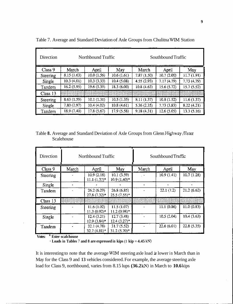
Table 7. Average and Standard Deviation of Axle Groups from Chulitna WIM Station

Direct ion Northbound Traffic Southbound Traffic

Table 8. Average and Standard Deviation of Axle Groups from Glenn fighway Ester Scalehouse

I Direction Southbound Traffic I Northbound Traffic I I

Votes: * Ester scalchouse - Loads in Tables 7 and 8 are expressed in kips (1 kip = 4.45 kN)

It is interesting to note that the average WIM steering axle load is lower in March than in May for the Class 9 and 13 vehicles considered. For example, the average steering axle load for Class 9, northbound, varies from 8.15 lups (36.2 kN) in March to 10.6 kips

10

(47.1 kN) in May (Table 7). This could be attributed to the sensitivity of the system to climatic change and frozen ground conditions. The WIM data also show very good agreement for steering axle weights averaged for a given month, indicating a good degree of “repeatability” for given climatic and ground conditions. The agreement between WIM and scalehouse data for average values of steering axle loads during April and May (i.e., the period when seasonal load restrictions are applied) is essentially within 10%. The large discrepancy for the WIM and scalehouse single and tandem axle weights could be a result of the different truck loads at the Glenn Highway and Chulitna and/or improper calibration of the WIM.

Comparisons between scalehouse and WIM data for this study indicate that major discrepancies occur for single and tandem axle loads (Tables 7 and 8). In this case, WIM data should be adjusted to be more compatible with scalehouse data. Since no “one to one’’ axle weight correlations were obtained for WIM and scalehouse traffic, the averages of the axle load distributions were compared for Class 9 and Class 13 vehicles. The ratio of the average scalehouse axle weight to the WIM axle weight is summarized in Table 9. Data in Table 9 were used to determine the average load ratios or factors in Table 10. These ratios were used to convert WIM axle loads to their corresponding scalehouse values. In this case, the corresponding adjustment between WIM and scalehouse EALs is 4.03 and 2.47 for northbound and southbound traffic respectively (i.e. scalehouse EALs is equal to WIM EALs times adjustment factor). These adjustment factors were obtained for 1993-1996 traffic data and applied for EAL computations in this report.

Table 9. Ratio Scalehouse to WIM Average Axle Loads

Direction I Northbound Traffic Southbound Traffic

I I I I

Steering 1.13 1.08 1.03 0.95 Single 1.22 1.16 1.36 1.26

Tandem 1.71 1.76 1.79 1.71 4

Table 10. Average Axle Load Ratios Used to Adjust WIM Axle Loads

Northbound Traffic Southbound Traffic

3.2 Axle Load Distribution

Analyses were performed on the collected WIM 1993-1996 data in order to determine the potential damage to the Parks Highway associated with truck traffic. In this case, the WIM data were converted to estimate scalehouse axle loads and EALs. The distribution of axle loads for Class 5- 13 vehicles and the corresponding EALs were determined. In addition, the percent axle overloads exceeding the 75% load restriction limit was estimated for different axle groups, and the influence of the axle overloads on pavement damage was assessed. Results of analyses are summarized in Appendix D. Since pavement damage is influenced by both climate and load applications, the distribution of axle loads with time for a given year was examined. Winter, spring, summer, and fall distributions for northbound 1995 traffic appear in Figures 1-12. For a given axle group, results indicate a general increase in axle loading magnitude and number of applications during spring and summer in comparison with fall and winter traffic. Maximum truck traffic, however, seems to occur during summer (July-September); the most signficant increase in number and load magnitude is associated with tandem axles.

Comparison between northbound and southbound traffic shows a similar trend in terms of seasonal distribution; however, as expected, the magnitude of the axle loads, particularly the tandem axles, is much lower. This is illustrated in Figures 13 and 14, whereby the number of Class 5-13 vehicles and EALs are compared for both north- and southbound traffic. As indicated, although the number of trucks are essentially similar (Figure 13), the maximum northbound and southbound EALs occur between June and August and are about four times as much for northbound traffic as southbound (Figure 14). The difference between southbound and northbound loading can also be illustrated by comparing the average monthly EAL per vehicle (Figure 15). It is interesting to note that the average

12

monthly EAL per vehicle varies between 0.5 and 1.5 for southbound traffic and between 1.6 and 4.8 for northbound traffic.

Analysis of the number of EAL resulting from traffic loads for Class 5-13 vehicles indicate that Class 13 vehicles yield the maximum EAL. This is illustrated by comparing the total monthly EAL for all vehicles with those corresponding to Class 13, as shown in Figures 16- 19. The average number of trucks per day is about 70 for both north- and southbound traffic (1995 data). The average EAL per vehicle (Class 5-13) is summarized in Table 11. It is interesting to note that for a given design E L , using the northbound EAL/veh. data in Table 11 will result in an expected design life that is about 17% longer if load restrictions are applied, compared to a pavement with no restrictions. The increased EAL associated with the 1996 lifting of load restrictions is also illustrated in Figures 16 - 23. Results indicate that maximum EALs occur during the months of June - August. It is interesting to note that, when restrictions were lifted in 1996, the April - May EAL increased from about 6,000 to 18,000 for southbound traffic and from 9,000 to about 25,000 for northbound traffic.

Table 11. Summary of EAL/Vehicle (Class 5-13) with and without Load Restrictions

3.3 Overload Damage Considerations

Analysis of axle overloads associated with truck traffic was performed for the period covering April fKst to mid-May, which corresponds to the period during which load restrictions are traditionally applied on the Parks Highway. Specifically, the analysis addressed the following:

1. What percent of each axle group is over the 75% allowable limit?

2. Of the total “spring-thawyy damage, what percentage does each axel group contribute?

3. What is the contribution of axle overload of each group to the total “spring-thaw” damage?

13

The analysis was conducted using WIM data from 1993-1996 for both northbound and southbound traffic. A summary of percent overload for each axle group, expressed as the ratio of the number of axles exceeding the allowable load limit to the total number of axles during the "spring-thaw period", is presented in Table 12. For northbound traffic the maximum overloads occur for the tandem axles and vary from an average of about 18% for the period when load restrictions were applied (i.e. 1993-1995) to about 32% when load restrictions were lifted in 1996. In other words, removal of load restrictions increased the number of tandem overloads by 14% of the total tandems during the spring-thaw restriction period. This corresponds to an increase in the number of tandem overloads of about 78%. Comparison of steering and single axle loads for periods when load restrictions were applied, with the 1996 traffic when restrictions were lifted, shows no significant decrease in overloads for northbound traffic. On the other hand, some decrease in overload is observed for southbound traffic, particularly for the steering axle loads.

Table 12. Percent Overload for Different Axle Groups during Spring-Thaw Period

Northbound Traffic Southbound Traffic

Notes: - Overload for steering axle group corresponds to axle loads in excess of 53.3 kN (12 kips) - Overload for single and tandem groups corresponds to axle loads in excess of 75% of maximum legal load (Table 4).

The effect of the relative damage caused by the different axle loads during the "spring- thaw" period was also determined by comparing the ratios of EAL associated with a given group to the total EAL applied. Similarly, the relative damage due to overload could be calculated by using the EAL of the overload associated with a given axle group. Table 13 summarizes the results of "spring-thaw" damage by different axle groups. Overload damage is presented in Table 14.

Comparison of damage induced by the different axle groups clearly illustrates that tandem axle loads are responsible for a significant portion of pavement damage during "spring- thaw". During 1993-1995, when load restrictions were imposed, about 87% of damage

14

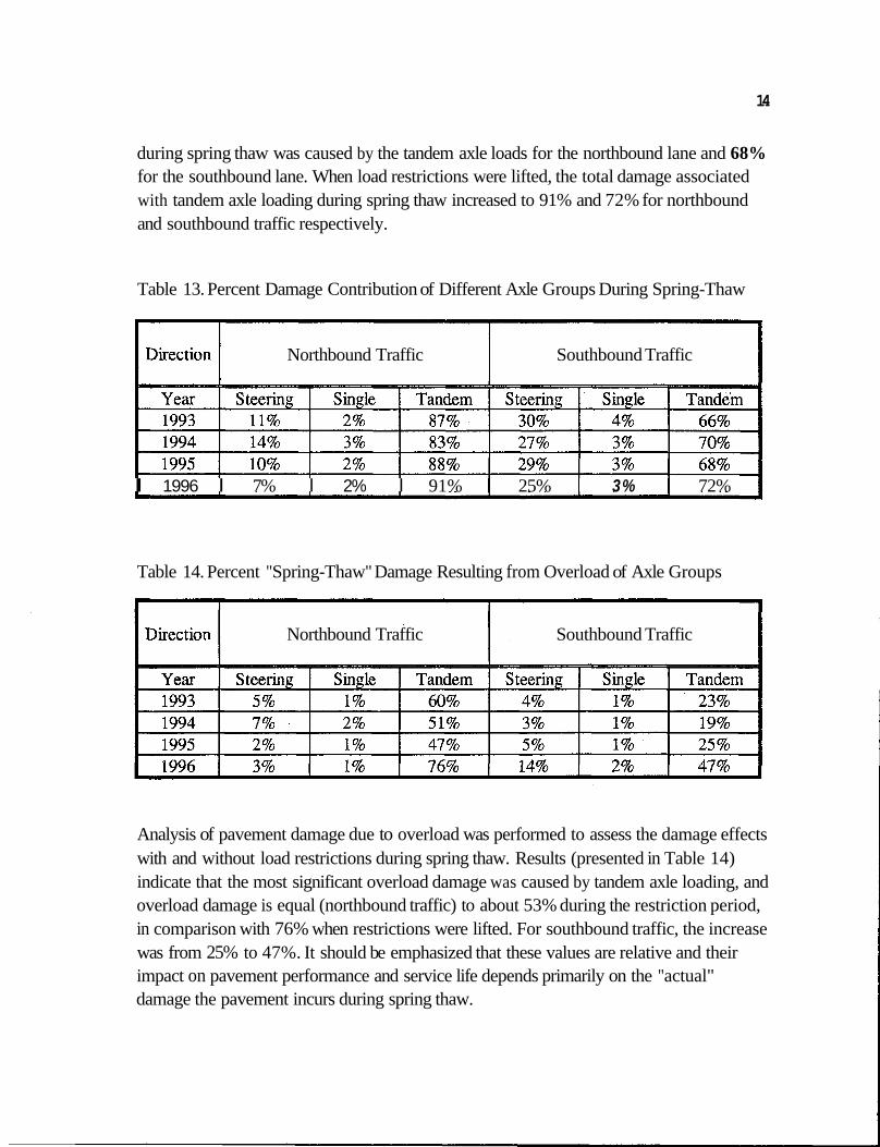
during spring thaw was caused by the tandem axle loads for the northbound lane and 68% for the southbound lane. When load restrictions were lifted, the total damage associated with tandem axle loading during spring thaw increased to 91% and 72% for northbound and southbound traffic respectively.

Table 13. Percent Damage Contribution of Different Axle Groups During Spring-Thaw

Northbound Traffic Southbound Traffic

I 1996 I 7% I 2% I 91% I 25% I 3% I 72% I

Table 14. Percent "Spring-Thaw" Damage Resulting from Overload of Axle Groups

Northbound Traffic Southbound Traffic

Analysis of pavement damage due to overload was performed to assess the damage effects with and without load restrictions during spring thaw. Results (presented in Table 14) indicate that the most significant overload damage was caused by tandem axle loading, and overload damage is equal (northbound traffic) to about 53% during the restriction period, in comparison with 76% when restrictions were lifted. For southbound traffic, the increase was from 25% to 47%. It should be emphasized that these values are relative and their impact on pavement performance and service life depends primarily on the "actual" damage the pavement incurs during spring thaw.

15

4, ANALYSIS OF GROUND TEMPERATURE DATA

Temperature data for the sites summarized in Table 5 were analyzed to determine thaw initiation and propagation in the pavement structure. This is sigruficant for load restrictions, since spring-thaw weakening of the pavement is influenced by the depth of thaw. In this case, accelerated distress associated with base failure or fatigue failure of the asphalt concrete surface could occur. Analyzing pavement structures of the Elliott and Haines highways (Raad et al. 1995) indicates that maximum damage in the unbound granular base course occurs when thawing initiates at the top of the base. The damage factor associated with spring-thaw weakening of the base remains high and critical until the thaw depth reaches about 0.6 meters (2 feet) below the pavement surface. On the other hand, the damage factor related to fatigue of the asphalt concrete surface increases gradually until it reaches a maximum for a thaw depth of about 0.6 m (2 ft), afterwhich it starts to decrease as the pavement gets dryer and stronger. According to a nationwide survey of numerous departments of transportation in the U.S. and Canada ( Raad et al. 1995), the critical thaw depth is on the average equal to about 1.2 m (4 ft). Based on both field observations and theoretical analysis, it is reasonable to assume that the critical thaw depth during which the pavement structure is most susceptible to spring-thaw damage is about one meter.

\

In this study, thaw initiation corresponded to the time at which thawing at the top of the granular base, about 12 cm below pavement surface, occurred. Thaw propagation was monitored by obtaining an hourly record of the thermistor string temperature readings at a given site. The variation of thaw depth with duration of thaw is illustrated in Figures 24- 30. Regression analyses were performed to develop thaw propagation relationships as a function of duration of thaw. These equations were expressed as follows:

Log (z) = a Log (t) + b (4)

where

z = Depth of thaw in mm t = Duration of thaw in days a,b = Constants for a given site

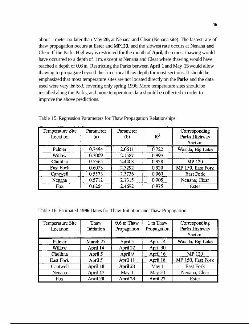
A summary of the constants a, and b in Equation 4 for the different sites is presented in Table 15. Thaw initiation and propagation results are shown in Table 16. The earliest thaw initiation occurs on March 27, at Wasilla and Big Lake (Palmer site), and propagates

16

about 1 meter no later than May 20, at Nenana and Clear (Nenana site). The fastest rate of thaw propagation occurs at Ester and Mp120, and the slowest rate occurs at Nenana and Clear. If the Parks Highway is restricted for the month of April, then most thawing would have occurred to a depth of 1 m, except at Nenana and Clear where thawing would have reached a depth of 0.6 m. Restricting the Parks between April 1 and May 15 would allow thawing to propagate beyond the lm critical thaw depth for most sections. It should be emphasized that most temperature sites are not located directly on the Parks and the data used were very limited, covering only spring 1996. More temperature sites should be installed along the Parks, and more temperature data should be collected in order to improve the above predictions.

Cantwell Nenana

Fox

Table 15. Regression Parameters for Thaw Propagation Relationships

April 18 April 23 May 1 East Fork April 17 May 1 May 20 Nenana, Clear A~ri l 20 A~r i l23 A~ri l 27 Ester

Table 16. Estimated 1996 Dates for Thaw Initiation and Thaw Propagation

17

5. ANALYSIS OF FIELD RUTTING AND ROUGHNESS

5.1 Field Observations of Pavement Distress during Spring: Thaw

The Parks Highway was monitored weekly from 15 April to 19 May during Spring 1996 to determine the effect of lifting load restrictions on pavement damage. The pavement between CDS Miles 35 and 315 was examined for distress modes that included bleeding, pot-holes, cracking, and rutting. These areas were short intervals not necessarily associated with the test section discussed in Table 2. When a given distress mode was first observed, its location was marked and its progression with time monitored. This would provide data on the most critical locations of the Parks and the type and extent of damage incurred during spring-thaw. Discussions with the maintenance foremen indicated that, in their opinion, these distress areas were not more severe than when load restrictions had been applied in the past. A summary of field data is included in Appendix C.

Rutting and bleeding were the most common forms of observed distress. Rutting occurred at critically "weak" locations and was generally accompanied by bleeding. The development of ruts was by no means "gradual" but occurred relatively quickly. The full depth of the observed ruts seemed to develop very soon after they were first observed, which indicates the occurrence of "soft" support condition (i.e. probably base failure) under the pavement surface. The depth of the ruts varied between 15 mm and 90 mm. Table 17 summarizes the type, date, and estimated thaw depth for the first observed distress mode. It is interesting to note that the first observed ruts occurred when the estimated thaw depth was between 0.3 rn (Nenana) and 1 m (Ester), which indicates that the assumption of a critical thaw depth of 1 meter is reasonable.

An attempt was also made to assess the influence of axle loads on observed damage by comparing the frequency and level of distress in the northbound and southbound lanes. Results are summarized in Table 18. Although the northbound traffic during the monitoring period (15 April to 19 May) results in 50% more EALs than southbound traffic, the average northbound rut is less than the average southbound rut. The total number of observed distress areas, though, were 30% more in the northbound lane.

18

Table 17. A Summary of Distress Observed for the Selected Field Sections on the Parks (Not necessarily associated with the test sections in Table 2)

General Date first Estimated Initial Rut Final Rut Selected Distress Rut Thaw Depth Depth

Site Depth (m> (mm>

I MP120 I None I - I - I - I - MP 150 Rutting 15April 0.85 18 18

East Pot Holes, 28 April 0.85 21 33 Fork Rutting,

Bleeding. Clear Rutting 19 May 0.98 49 49

Nenana Rutting, 21 April 0.30 58 70

Ester Rutting, 15 April 1 .o 49 52 Pot Holes

Pot Holes, Soft Areas

Table 18. Comparison of Northbound and Southbound Observed Distress (Not necessarily associated with the test sections in Table 2)

5.2 Profdometer and Rut Bar Measurements

Roughness and rutting data for the Parks Highway were analyzed to determine the following:

1. An estimation of how much damage occurs during the spring-thaw period as a result of load restrictions.

19

2. An assessment of the influence of "reduced" magnitude of axle load exerts on pavement damage, conducted by comparing rutting and roughness of northbound and southbound lanes.

3. A determine of the accumulation of "yearly" damage for 1993- 1996 traffic and develop corresponding damage relations for roughness and rutting as a function of EAL.

Results of profilometer rut and roughness measurements conducted between 4/24/96 and 7/2/96 are summarized in Tables 19 and 20. Both average and standard deviation values for the Parks sections are presented. Rut bar measurements over spring thaw were conducted at specific locations periodically between 3/12/96 and 5/27/96. Average and standard deviation for each section are summarized in Tables 21 and 22.

Analysis of rut and roughness data indicate the following:

1. Average profdometer rut and roughness measurements in the northbound lane obtained on 4/24/96 are generally larger than rut measurements obtained on 7/2/96 (Table 19). One possible explanation could be that climatic effects associated with frost heave are more significant than load effects for the current traffic level @e., about 70 trucks/day, and estimated 300 EAL/day).

2. Profdometer rut values for 7/2/96 are generally larger for the southbound lane than the northbound lane, although southbound EALs are about 70% smaller. One possible explanation for this could be that the dynamic effect of "lighter" loads is more significant than "heavier" loads, thereby resulting in more road damage. In other words, for a given truck "suspension system," heavier loads could be more "dampened" than "Lighter" loads. Conventional methods for pavement design and analysis do not properly address this issue. Another possibility could be the poor drainage along many south-facing cut sections on the Parks, which puts the southbound lane on the uphill side of the cut. More research is needed to evaluate vehicle dynamic effects and climatic effects on pavement damage.

3. Comparison between northbound and southbound IRI for the 7/2/96 data indicate essentially no significant difference.

20

in n

a z

21

3 4

n

W

c3

W

>

4

2

Z

0

€+

Y

d

h-

z5

-w

22

Ir

o

am

rn I- a

23

24

4. It is interesting to note that although profilometer ruts for the southbound lane are larger for 7/2/96 than 4/24/96, the IRI is smaller, indicating a smoother "ride". This could indicate the more "pronounced" compaction effect associated with vehicle dynamics following ground thawing.

5. Rut-bar data show no significant pavement damage during spring thaw as a result of lifting seasonal load restrictions (Tables 21-22). Average values of southbound ruts for 5/14/96 are generally larger than northbound ruts. Such a trend, however, was not observed for earlier dates.

6. "Yearly" proflometer rutting and roughness data for 1993, 1995 and 1996 were compared with "seasonal" data obtained during spring 1996. Typical results appear in Figures 31-34. Higher IRI values were measured in spring. Rutting, on the other hand, seems to decrease in May, which might indicate a decrease in differential heave as a result of thawing. The follow-up increase of rutting July is load-related.

7. Yearly proflometer rutting and roughness obtained in 1996 for the northbound lane were compared with the southbound lane measurements. Results are presented in Table 23. In this case, the variation of rutting and IRI with EAL was 'determined for the northbound, then compared with rutting and IRI for the southbound lane (Figures 35-42). Results clearly illustrate that the southbound lane exhibits more damage than the northbound.

5.3 Damape Models

Damage models for rutting and roughness were developed for the Parks sections in this study. The aim of these models is to predict roughness (IRI) and rutting performance with EAL. After examining the available data, it was concluded that proflometer yearly data (1993, 1995, and 1996) were the most suitable since seasonal data in most cases did not show any increase of rutting or roughness with applied EAL. Yearly data were also selected so that only sections that showed increase in rutting and roughness were considered. Since the data were quite limited, an incremental approach to predict the change in rutting and IRI with E L was used. This would allow extrapolation of the relationships by integration.

The incremental relationships are summarized in Tables 24 and 25. In this case, the stiffness (E) for the pavement layers of each section corresponds to the average spring and

25

..

6.05 - -

Table 23. Comparison of Northbound and Southbound Rutting and IRI

1.41 -

1.54 1.44

- 6.22

- -

1.59 -

1.80 1.75

Rut Ikm) SB Section NB EAL

0 85324 148659 271 666

0 85324 148659 271 666

0 85324 148659 27 I 666

0 85324 148659 27 1 666

0 85324 148659 27 1 666

0 85324 148659 27 1 666

0 85324 148659 271 666

0 85324 148659 271666

9.95

7.22 5.33 5.44

5.93 6.10 4.1 1

2.54 5.78

-

-

-

Wasi I la 6.22 - 1.30

1.60 - 1.80

- 1.95

2.55 - I .31

1.26 1.69

- 1.38

- I .36 - 1.41

9.70 -

6.35 -

7.92 -

Big Lake

MP 120-125

5.38

2.12 7.03

- MP 150-155

East Fork 5.94

5.57 6.40

- - 1.73

- 1.81 - 1.94

9.14 -

4.78

9.53 7.32

- 1.80

- 2.01 - 1.96

9.40 - Clear

2.44

1.54 4.93

- - I .47

- -

Nenana

3.43

3.35 5.59

Ester

. 26

Table 24. Regression Coefficients for Incremental Rutting Damage Model

BigLake

East Fork

Clear

Nenana

Ester

Regression Coefficients for

log y = a + b.log x1

where : y = dei.Rut, mm

XI = del.EAL

-2.503

10.91 4

-22.287

-3.846

-1 3.160

Section I a

0.2535

-2.3200

4.1 580

0.5872

2.2795 I

Table 25. Regression Coefficients for Incremental IRI Damage Model

Regression Coefficients for

log y = a + b.log x1 + c.log x2

where : y = del.lRI , m/Km

x1 = del.EAL

x2 = sum(E.!) , MPa.m

Section

Wasilla

BigLake

MP120

East Fork

Clear

Nenana

Ester

a

-3.570

-1.716

-1 7.432

-10.159

-14.527

-21.632

-1 1.006

b

1.0065

0.5263

3.1760

2.1 764

2.751 6

3.901 5

1.8270

C

-0.8405

-0.6424

-0.8733

-0.3385

27

summer values obtained from FWD backcalculation using ELMOD (Ullidtz 1987). Layer thicknesses for the different locations are summarized in Table 26. In determining (sum (E.t)), the lower pavement boundary was assumed to be equal to the depth of the backcalculated "stiff" layer. A terminal rut and IRI of 25 mm and 6 m/km respectively were used in the derivations.

The extrapolated relationships are summarized in Tables 27 and 28. They predict the development of rutting and IRI with EAL starting with a "new" pavement (initial rut = 0, and initial IRI = 1 m/km). The variation of rutting and IRI with EAL is illustrated in Figures 43-44. It should be emphasized that these relationships have a number of limitations, including:

1. The relationships were developed using very limited data. Future rutting and IRI data could be used to obtain improved correlations.

2. The relationships included sections that exhibited increased rutting and IRI with EAL. It is therefore expected that predictions could be conservative, since rutting and IRI for some sections did not increase with applied EAL.

3. Because of the lack of "good" data, rutting and IRI damage functions could not be developed for all selected sections of the Parks.

Rut and IRI predictions using the developed relationships were compared with 1993 data (Figures 45-46). Results indicate that predicted values are, on the average, twice the measured rutting values and 1.4 the IRI values.

6. ANALYSIS OF FWD DATA AND STRUCTURAL CONSIDERATIONS

Generally backcalculation analysis is conducted to estimate pavement layer moduli and damage factors from surface deflection measurements. Of particular interest in this study is the determination of pavement structure "weakening" during spring thaw and the corresponding loss of pavement service life. Mechanistic analysis of pavements indicate that spring-thaw damage is mainly associated with fatigue of the asphalt concrete surface or failure of the underlying granular base (Raad et al. 1995). Critical damage factors for the Elliott Highway granular base have been found to vary between 10 and 30; for the Haines Highway, between 2 and 6 (Raad et aL 1995). Based on results of multilayer analysis by Raad et al. (1997), estimates of base damage factors for conditions similar to the Parks Highway are expected to vary between 5 and 10.

Table 26. Pavement Thickness for Parks Highway Sections

28

Parks Highway

Pavement Thickness

I Section

Wasilla

Big Lake

MP120-125

MP150-155

East Fork

Clear

Nenana

Ester

Votthbound

76

89 '

102

76

58

58

61

56

Southbound

76

1 02

1 27

76

58

58

61

56

Base Thickness at all locations is 1067 mm

Table 27. Regression Coefficients for Rut versus EAL Model

Regression Coefficients for

Predicted Rut (mm) = a.x + b.x2

x = EAL in thousands

29

1815

1134

200

632

Table 28. Regression Coefficients for IRI versus EAL Model

1.096 2.320E-03 -3.364E-07 0.999

1.024 3.530E-03 -8.643E-07 0.999

1.030 3.798E-03 -9.804E-07 0.999

1.052 1.503E-03 -1.503E-07 0.999

r- Section

I Wasitla

Big Lake

MP 120-12:

I Nenana

1 Ester

Regression Coefficients for

Predicted IRI (m/Km) = a + b.x + c.x2

x = EAL in thousands

Sum(E.t)

MPa.m

~~ ~~~

131 1 I 1.057 1 1.552E-03 1 -1.588E-07 I 0.999

665 1 1.039 I 1.367E-03 I -1.276E-07 I 0.999

562 I 1.014 I 9.612E-041 -6.885E-08 I 0.999

FWD results are presented in Appendix F. Average values for damage factors (fatigue of asphalt concrete), and layer moduli determined from FWD analysis are shown in Figures 47-54 for selected sections on the Parks. These results indicate the following:

I . Average damage factors for both northbound and southbound lanes are essentially similar; they vary during spring-thaw between 0.4 and 8. The average damage factor per mile is generally less than 2, except for East Fork, where it reaches 8 in some locations. In this case, a damage factor less than 1 indicates that more summer damage occurs as a result of EAL application than during spring thaw.

2. The backcalculated depth to "stiff layer" obtained between late March and early May varies between 0.5 m and 1.3 m. This is larger than the expected depth of thaw predicted from ground temperature data. It should be emphasized, in this case, that the depth to stiff layer determined by ELMOD is an "equivalent" depth calculated using Odemark formulation (Ullidtz 1987). It is likely that the backcalculation overpredicts the actual thaw depth in pavements.

30

3. Reducing the applied load from 9 kips (40 kN) to 7 kips (31.1 kN) will reduce the damage factor on the average by about 0.5 to 0.8. On the other hand, increasing the applied load from 9 kips (40 kN) to 14 (62.3 kN) kips will increase the damage factor from about 2.4 to 3.

4. Results presented in Figures 47-54 illustrate the variation of layer moduli and damage factor during spring thaw. in most cases the thaw-weakening effects are apparent on the base and subgrade inocluli. For the asphalt concrete layer, the backcalculated modulus in early spring is "lower" than predictions obtained from temperature relations. This may reflect a localized weak base condition associated with base thawing.

The influence of load restriction on remaining pavement service life has been deterinined as part of this study. In this case, the r e m ~ i i n g service life depends on the damage factor associated with spring-thaw weakening, and the applied EALs. A simple derivation was developed, in this case, where pavement life with load restrictions is coinpared with expected life if restrictions were removed. The proposed model uses basic principles of pavement analysis and accounts for cumulative damage using Miner's hypo thesis. The remaining life ratio (r), defined as the ratio of pavement service life withuut load restrictions to service life with restrictions, can be expressed as follows:

r = [k (DF) + 11 / [k (1+A) DF + I ]

Where

(5)

k = Ratio of EAL during the restriction period to the remaining applied EALs when restrictions are removed, over a perjod of one year

DF = Average damage factor during the restriction period

A = Change of EAL as a result of removing load restrictions divided by the total EAL when restrictions are applied (note that the EALs in this case are for the assumed critical spring-thaw period over which restriction are generally applied).

31

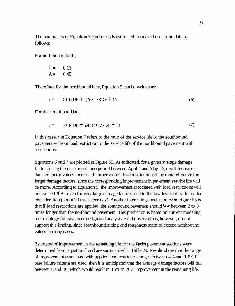
The parameters of Equation 5 can be easily estimated from available traffic data as follows:

For northbound traffic,

k = 0.13 A = 0.45

Therefore, for the northbound lane, Equation 5 can be written as:

r = (0.13DF + 1)/(0.188DF + 1)

For the southbound lane,

r = (0.46DF + 3.44)/(0.27DF + 1) (7)

In this case, r in Equation 7 refers to the ratio of the service life of the southbound pavement without load restriction to the service life of the northbound pavement with restrictions.

Equations 6 and 7 are plotted in Figure 55. As indicated, for a given average damage factor during the usual restriction period between April 1 and May 15, r will decrease as damage factor values increase. In other words, load restriction will be more effective for larger damage factors, since the corresponding improvement in pavement service life will be more. According to Equation 5, the improvement associated with load restrictions will not exceed 30%, even for very large damage factors, due to the low levels of traffic under consideration (about 70 trucks per day). Another interesting conclusion fi-om Figure 55 is that if load restrictions are applied, the southbound pavement should last between 2 to 3 times longer than the northbound pavement. This prediction is based on current modeling methodology for pavement design and analysis. Field observations, however, do not support this finding, since southbound rutting and roughness seem to exceed northbound values in many cases.

Estimates of improvement in the remaining life for the Parks pavement sections were determined from Equation 5 and are summarized in Table 29. Results show that the range of improvement associated with applied load restriction ranges between 4% and 13%. If base failure criteria are used, then it is anticipated that the average damage factors will fall between 5 and 10, which would result in 15% to 20% improvement in the remaining life.

32

Table 29. Estimated Improvement in Remaining Life Resulting from Load Restrictions

Length of the critical thaw period during which load restrictions may be applied depends on the rate of thaw propagation. However, the level of load restriction depends on the damage factor, which is influenced by the "weakening" of the pavement structure during spring thaw. The decision to apply load restrictions depends to a great extent on the resulting benefits or improvement in remaining pavement life. For this purpose, a graphical method, developed as part of this study, obtains a quick estimate of remaining life improvement should seasonal restrictions be applied. In this case, northbound traffic was used to estimate the value of (k) in Equation 5 for a given restriction period (d, days) as follows:

k = 0.001815 (d)/(l - 0.001815d) The improvement in remaining life, p can be written as

p = 1-1- (9)

Substituting for (r) in Equation 5 and solving for DF yields:

Using A = 0.45, then, for a given p the relationship between DF and (d) can be determined. Such relationships -- for p between 0.05 (5% improvement) and p = 0.25 (25% improvement) -- are presented in Figure 56. The application of Figure 56 is simple and useful. For example, if the average damage factor is determined from FWD tests,

33

and the duration of thaw associated with about 1 meter thaw into the pavement is estimated from ground temperature data, then the resulting benefit or improvement in remaining life can be directly estimated from Figure 56. On the other hand, if the improvement in remaining life is used as a criterion for seasonal restrictions, then the limiting damage factor below which no restrictions are required could be easily determined.

Strengthening existing weak sections so that they could withstand truck traffic without seasonal restrictions could be considered as an alternative to seasonal load restrictions. The following section was designed by Raad et al. (1995) and is applicable for the Parks:

100 mm of HMA 150 mm of open-graded base, preferably bituminous treated 600 mm of non-frost susceptible subbase

The use of asphalt concrete surface thicknesses of at least 100 mm is recommended, because of the significant reduction of accumulated damage during spring thaw. This is illustrated in Figure 57, which shows the variation of damage consumption factor (i.e. the consumed damage of the pavement during spring per 1000 EAL applications) with thickness of asphalt concrete layer. Results show significant reduction in consumed damage for both the asphalt concrete layer (fatigue) and the granular base (base failure).

7. SUMMARY AND CONCLUSIONS

In this report is an attempt at determining the effects of lifting seasonal load restrictions on the Parks Highway in 1996. Extensive analysis of field data including traffic, ground temperature, rut and roughness measurements, and structural analysis using FWD backcalculation procedures were performed.

Traffic analysis indicated that truck traffic averaged about 70 trucks per day with an average EAL per truck equal to 0.95 when load restrictions are applied and 1.1 1 EAL per truck when load restrictions are lifted. The maximum improvement of remaining pavement life resulting from restricting loads is about 15%. Mechanistic analysis using backcalculation procedures predict remaining life improvement between 4% and 13% for the asphalt concrete layer and 15% to 20% for the granular base. Procedures were developed to estimate the increase in remaining pavement life for a given damage factor and restriction period. In addition, damage functions for rutting and IRI were developed

34 ..e

as part of this study to bvestigate the long term performance of different sections of the Parks. These functions were based on very limited data and seem to overpredict rutting by a factor of 2 and IRI by a factor of 1.4.

One of the most interesting findings was that the southbound lane, which carries about 70% less EALs than the northern lane, exhibits more damage. A possible explanation in this case is related to pavement-vehicle dynamics. The dynamic effects of "lighter" traffic on pavement damage could be more significant than those of "heavier" traffic. Current methods of pavement analysis and design do not seem to address this issue properly. In fact, pavement dynamics are not properly accounted for in conventional design procedures. Another explanation could be related to a drainage problem with south-facing cut slopes along the Parks. Analysis of causes for the difference in observed damage was not within the scope of this study, and further work is necessary to address such issues.

Another interesting observation was the significant influence of climate on pavement damage. Extensive profdometer and rut bar measurements during the critical spring-thaw period show that many of the sections observed are "rougher" and have "deeper" ruts in early spring than late spring. This is contrary to expectations since load restrictions were lifted during the period of observation, and the pavement is expected to be "damaged" more at the end of the spring-thaw period than at the beginning. A possible explanation of these observations is that climatic damage resulting mainly kom frost heave is significant relative to the "light" traffic conditions applied to the pavement structure. Should traffic conditions increase, then the climatic effects could become "relatively" less severe, and the pavement will show more load-associated damage. Proper determination of the traffic level and load limits required to induce detrimental effects on pavement damage again calls for additional research efforts.

35

8. REFERENCES

Raad, L., Coetzee, N., and Hicks, G. R. Load Restriction Criteria for Alaskan Roads: Phase 1: General Considerations and Field Studies. Report No. INEDRC 24. 94 (Draft), Institute of Northern Engineering, Transportation Research Center, University of Alaska Fairbanks, September 1995.

Raad, L., Minassian, G., and Saboundjian, S . Mechanistic Evaluation of the Effect of Tire Inflation Pressure on Pavement Damage under Spring-Thaw Weakening. Transportation Research Board Meeting, Washington, D.C., January, 1997.

Schook, J.F., Finn, F.N., Witczak, M.W., and Monismith, C.L. Thickness Design of Asphalt Pavements - The Asphalt Institute Method. Proceedings, The Fifth International Conference on Structural Design of Asphalt Pavements, Delft, 1982.

Ullidtz, P. Pavement Analysis. Elsevier, 1987.

FIGURES 1 - 56

37

m

S

Q)

Q)

.I

L

U

v)

0

0

v)

N

cs r

I

v)

0

0

0

cv

0

0

v)

r

0

0

0

r

0

0

u)

38

I

0

0

u)

cv

0

0

0

cv

0

0

u)

r

0

0

0

r

0

0

0

v)

39

c)

r

I

v)

0

0

0

0

0

0

0

0

0

0

0

0

0

0

0

0

0

v)

0

v)

0

v)

0

v)

d

M

M

cy cy

r

r

0

SalX

v fiU!.laaJS 4

0 'O

N

40

0

0

m

r

0

0

0

r

0

0

m

0

41

0

0

to 0

0

u)

0

0

d

0

0

cy 0

0

r

(D

cy

s cy cy

0

cy

00 r

(D

F

d

r

cy r

0

r

00

Lo

d

cy

0

0

42

0

0

0

N

m

v= I

v)

0

0

m

'c

0

0

0

v=

0

0

m

0 0

cs

00 N

co cy

s cy N

0

cy

00 r

co r

d

r

cy r

0

r

03

co

d

cy

0

43

0 0

v)

m

cc) r

I

v) 0

0

0

m

0

0

0

0

0

0

0

0

v)

0

cy N

0

v)

r

r

0

0

0

v)

eo cy

(D

cy

s N

N

0

N

eo r

(D

r

d

r

N

r

0

r

00

(D

d

N

0

44

m

r

I

In

0

0

0

0

0

0

0

d

m

0

0

N

0

0

0

0

0

0

0

00 I-

W

v)

0

v.

00 N

W

N

3 \

N

N

0

N

00 F

(D

r

d

r

N

T

0

F

00

(D

d

N

0

45

Pa

(D

l-

v)

S

0 .I

.c

v)

n

u) U

Y

.I

Y

io’ Q

) Q

)

Q)

S

v

L

.c,

ICI Q

, P

a a 0

Pa

Pa

5 L l-

cu E

z a - C F

Pa

I I

0

0

0

0

0

00

0

0

(D

0

0

d

0

r

46

0 0

v)

F

0

0

N

F

0

0

m

0

47

0

0

v)

c-

, I

0

0

(v

c-

0

0

Q)

0

0

(D

0

0

c3

0

48

0

0

ua r

ua I-

M

r

I

ua

I

0

0

el T

0

0

M

0 I- v

)

ro

n

i

r- el

F

el

M

a

cb

2 Pi 3

a2

50

Ii

//

I I

/

/

I /

I

li I I I I \

I I i

i I

I I

I I

I I

I I

I I I

I IL

I I

I-

00

00

00

00

00

0

00

00

00

00

0

00

00

00

00

C

oc

Dw

NO

ma

wN

.

cY

v?

r

51

0 0

uj

0 0

c4 0 0

c\i

/

/

\ r I 0 0

.c

0 0 0

52

S

0 .I

0

0

0

0

0

0

0

CT)

cy cy

F

0

0

v)

0

0

0

0

0

0

v)

m

r

Om

0

0

0

0

0

v)

d

d

0

Om

0

0

0

v)

53

0

0

v)

N

0 0 0

N

0

0

0

F

0

0

v)

0

54

C

0 .I

.c,

J

0

I

0 0

0

4 4 0

0

co 0 ! 3

4 3 3

d- I 3 3 3

N

m

VI

M

I

55

0

0

0

0

0

0

0

0

0

0

0

0

0

0

0

v)

0

0

0

CD

0

0

0

00 I-

s m

(v

v-

0

0

0

L

Y

rn .C

I

2 w

56

C

0

3

9

ua J

W

.I

.cI

.I

L

.cII

.I

n

a

I

c9 r

I

ua 0

0

0

(v

0

0

0

d

0

0

0

(v

m

Vl

3

I

m

m

T

c1

c,

m

.* n

2 w

57

M

r

I

m

&

&

c-4

.-. 5 R

0

0

0

0

0

0 0

0 0 0

M

0 0

N

0 0 0

d

0

0

0

0

co v

)

0 0

0

r- t-

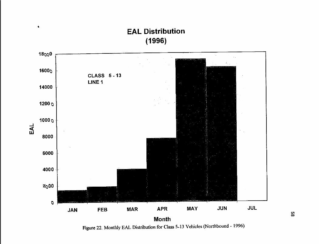
58

Pa r

I

v)

L

0

0

0

0

0

0

0

d

0

0

w

r

r

00

0

0

0

0

0

0

0

N

0

0

0

0

0

(D

d

0

0

0

00

0

0

0

0

0

N

.c

r

r

m

m

d

I

$ w

59

S

0

3

P

v)

ml

w

.I

*

..I

L

CI

8-

n

a m

v I

0

0

0

co

0

0

0

d

0

0

0

cv

lV3

cn * a n a

O

r

+

F 60

0

0

F /.

0

F

F

61

f 5 L 0 I I 0

0

0

0

F

0

0

0

0

0

r

W

F

0

F

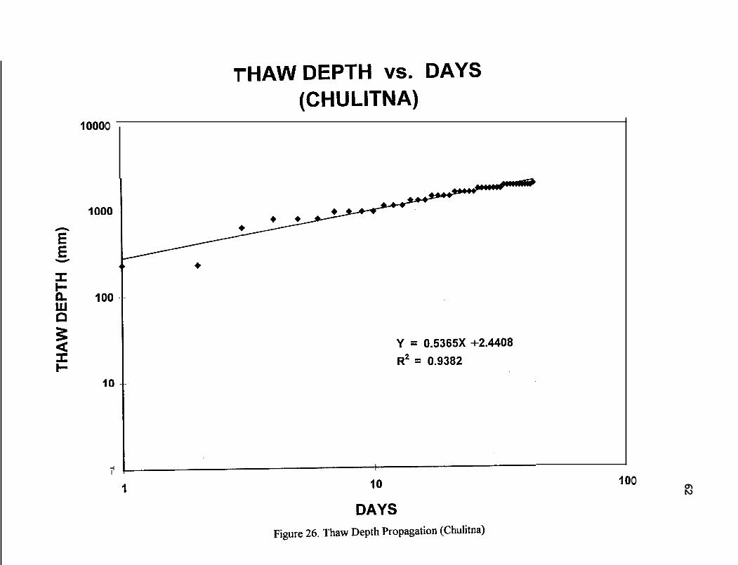
62

cn )I a

n n

3

a

z

I-

O

0

0

0

F

+ I1 ”

*?Y

0

0

r

T- O

0

r

0

r

F

3-

a =I= I-

O

0

0

F

N

03

cy

N

+ c?

64

cn ). a

n n

3”

a

I: I-

O

0

0

0

F

0

0

0

T-

0

r

+

0

0

0

v

0

0

F

a-

0

0

0

0

F

0

0

0

r

c*i +

Parks Hwy. - MPl20-125 Section 67

- 1 z

0

CDS 87

3%

0

I ) _ _ _ ?

1993 1995 4/24/96 5/8/96 7/2/96

CDS 88 1

- 9 ’ S l

0 1993 1995 a496 38/96 7 m

CDS 89 3 ,

Figure 3 1 . Comparison of Yearly and Seasonal IRI (Mp 120 - Northbound)

Parks Hwy. - CLEAR Section

4 -

68

i 2 -

03

f 3 . - - - - - - - -

- 1 - - - - - -

CDS 242

4

1993 1995 4/24/96 5/8196 7/2/96

CDS 243

5'

1993 1995 4/24/96 5/8/96 7/2/96

$ 2 - 1

0 1993 1995 4/24/96 5/8/96 7/2/96

CDS 244

4 1 I

1993 1995 4/24/96 5l8J96 7/2/96

1993 1995 4/24/96 5/8/96 7I2M

Figure 32. Comparison of Yearly and Seasonal IRI (Clear - Northbound)

69 Parks Hwy. - MP120-125 Section

CDS 86 7 7

6 6

5 5

CDS 85

E 4 E 4 i 3 $ 3

2 2

I I

0 0 1993 1995 4/24/96 5/8/96 7/2/96 1993 1995 4/24/96 5/8/96 7/2/96

CDS 87 7 . i

CDS 88 1

6

5

1 4 i 3

2

1

0

6

5

E 4 3 3

2

1

0 1993 1995 4/24/96 5/8/96 7/2/96 1993 1995 4/24/96 5/8/96 7/2/96

CDS 89 7 6 n 5

z 3 2

1

0 1993 1995 4/24/96 5 1 m 7 1 m

Figure 33. Comparison of Yearly and Seasonal Rutting (MI? 120 - Northbound)

70 Parks Hwy.- CLEAR Section

CDS 242 CDS 241 12 12

10 I O

E 8 E 8 - 6

e 4 5 $ 4

- 6

2 2

0 0 1995 1995 4/24/96 5/8/96 7/2/96 1993 1995 4/24/96 5/8/96 7/2/96

CDS 243 1

CDS 244 l2 u

3

1993 1995 4/24/96 518M 7/2/96 1993 1995 4/24/96 5/8/96 7/2/96

CDS 245 12

10

I 8 - 6

3 4

2

0 1993 1995 4/24/96 5/8/96 7/2/96

Figure 34. Comparison of Yearly and Seasonal Rutting (Clear - Northbound)

71

2.5

2 n

E : I

0.5

0

Y

z

Parks Hwy. = Wasilla

4 Northbound w Southbound

0 1 00,000 200,000 300,000

EAL (Starting from 1993)

Parks Hwy. - Wasilla 12 t I O

8

6

4

2

0

-0- Northbound Southbound

0 1 00,000 200,000 300,000

EAL (Starting from 1993)

Figure 35. Comparison of Northbound and Southbound IRI and Rutting (Wasilla)

72

Parks Hwy. - Big Lake

2.5 -E- 2 c

-0- Northbound = Southbound

0 1 00,000 200,000 300,000

EAL (Starting from 1993)

Parks Hwy. = Big Lake 12

10 : - - 8 f

6 ; CI - 4 : + Northbound 2 : w Southbound

o - ~ " " l n ' I n ' ' '

- 0

- 0 100,000 200,000 300,000

EAL (Starting from 1993)

Figure 36. Comparison of Northbound and Southbound IRI and Rutting (Big Lake)

73

Parks Hwy. = MP 120-125

-0- Northbound U

z 0.5 1 rn Southbound 0 E - I ' ' ' I ' I ' I ' I ' 0 100,000 200,000 300,000

EAL (Starting from 1993)

Parks Hwy. - MP 120-125

n

E E

5 Y

p.

E .c,

12 10 : 4 Northbound

Southbound 4

0 100,000 200,000 300,000

EAL (Starting from 1993)

Figure 37. Comparison of Northbound and Southbound IRI and Rutting (MP 120)

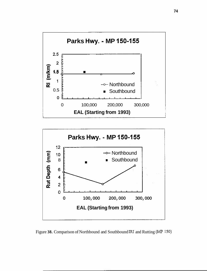
74

Parks Hwy. - MP 150-155

2.5

E E n 2 [ 1.5

0.5

U

z L

-0- Northbound Southbound

0 m 0 100,000 200,000 300,000

EAL (Starting from 1993)

n

E E

5 v

Q

E CI

Parks Hwy. - MP 150-155

-0- Northbound 8 rn Southbound

0 100,000 200,000 300,000

EAL (Starting from 1993)

Figure 38. Comparison of Northbound and Southbound IRI and Rutting (MP 150)

75

2.5

2

1.5

1

n

E

E v

z 0.5

0

Parks Hwy. - East Fork

+Northbound Southbound t

0 1 00,000 200,000 300,000

EAL (Starting from 1993)

n

E E

5 v

LI

E .c,

12

I O

8

6

4

2 0

Parks Hwy. - East Fork

-0- Northbound Southbound

0 100,000 200,000 300,000

EAL (Starting from 1993)

Figure 39. Comparison of Northbound and Southbound IRI and Rutting (East Fork)

76

- - - - - +Northbound

- Southbound - -

- 1 1 , 1 1 1 1 1 1 1 1 1 1 l

Parks Hwy. - Clear

1 2.5 t I 2 n

E 2

1

0.5

0

Y

I

p1

I- I D h - 0

Parks Hwy. = Clear

l2 1

rn Southbound 2 : o - l l I I " ' a " I ' l '

0 100,000 200,000 ~00,000

EAL (Starting from 1993)

Figure 40. Comparison of Northbound and Southbound IRI and Rutting (Clear)

77

Parks Hwy. = Nenana

1.5 S L

I

PL - 0.5 -0- Northbound Southbound

0 100,000 200,000 300,000

EAL (Starting from 1993)

Parks Hwy. - Nenana

n

E IO

8 E

5 6 e

v

Q) n 4 .c, z 2

0

-0- Northbound Southbound I

0 100,000 200,000 300,000

EAL (Starting from 1993)

Figure 41. Comparison of Northbound and Southbound IRI and Rutting (Nenana)

78

n

E z Y

z -

Parks Hwy. - Ester

2.5 2

I .5

1

0.5

t - 0

+ Northbound H Southbound

0 100,000 200,000 300,000

EAL (Starting from 1993)

A

E E

5 v

p.

c, z

Parks Hwy. - Ester 12

-0- Northbound H Southbound

0 1 00,000 200,000 300,000

EAL (Starting from 1993)

Figure 42. Comparison of Northbound and Southbound IRI and Rutting (Ester)

79

ua cy

It + 9 + $1 0

cy 0

F

ua

0

0

0

F

0

0

Q)

0

0

00

0

0

r- 0

0

(D

0

0

ua

0

0

d

0

0

rn

0

0

(Y

0

0

r

IO

0

80

.. I.

I L

I I

I I

I I

co rf)

d- rn

cv F

0 0

0

0

?

0 0

6,

0

0

00

0

0

b

0 0

co

0 0

u)

0

0

d-

0

0

c9

0 0

cv 0 0

T

0

81

\ I

H

4

X

*

X

82

Q)

Y

Q

,I

CI) .I

rn

E 0

L

v)

Q

W

.w

L

Q

Q)

23 0

4

X

M e

6

v)

d

c9

cv T

0

83

WASILLA - CDS MILE 13 NORTHBOUND

MODULUS VARIATION

14000

12000

- 10000 8000

h VI =! 2 =) 6000 0 0 Z 4000

2000

0 l-Mar 20-Apr 9-Jun 29-Jul

MODULUS VARIATION

[ -0-Ebase +Esubgrade 1

400 -

350 -

E, 300 - VI 3 250 -

2 200 -

p 150 -

100 -

50 . 0 1 l-Mar 20-Apr Wun 2Wul

DAMAGE FACTOR

1 .oo 0.90

0.80

0.70

0.60

0.50

t ri w 0.40 3 0.30 3 0.20

0.10 { 0.00 4

16-Mar SApr 25-Apr 15-May QJun 2 4 u n 1 4 u l

Figure 47. Typical Backcalculated Moduli and Damage Factors for Wasilla Section

84

BIG LAKE - CDS MILE 19 NORTHBOUND

I MODULUS VARIATION I+Eac

16000 1

14000

12000

10000

- s v)

3 0 6000 0 ' 4000

2 8000

+

I 26-Mar 15-May N u l 23Aug

I

MODULUS VARIATION I +Ebase -R-Esubarade 1

300

250

200

v) 3 150 3 0

z

p 100

50

26-Mar 15-May eJul 23-Aug

DAMAGE FACTOR 1.6

0.0 4 M P r 2SApr 1 M a y 4 3 u n 244un 14Jul

Figure 48. Typical Backcalculated Moduli and Damage Factors for Big Lake Section

85

MP 120 - CDS MILE 88 NORTHBOUND

MODULUS VARIATION

50000

45000

40000 - 35000 30000

25000

h

2 20000 0 I 15000

(+Eac

l-Mar PO-Apr SJun 29-JuI

MODULUS VARIATION I -0-Ebase +Esubgrade I

700 1 600

- 500

5 400 v) 3 A

L

2 300 0 = 200

100

~~ ~ - ,

1 Mar 20-Apr W u n 29JuI

2.5

2.0 f

1.5

i

3 w 1.0 (3

4 0.5

DAMAGE FACTOR

L

25-Apr 1 M a y eJun 244.111 l4-Jul

Figure 49. Typical Backcalculated Moduli and Damage Factors for M p 120 Section

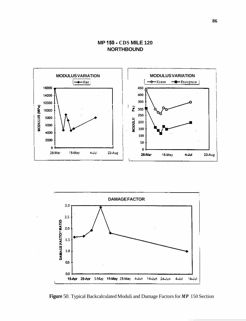
86

MP 150 - CDS MILE 120 NORTHBOUND

MODULUS VARIATION 1 +Eac i

0 2War IS-May Wul 23dug

MODULUS VARIATION r --B-Ebase +Esuborade I

450

400

350

6 300 250

3 5 200 n 8 150

100

50

0 26-Mar 15May 4 4 1 23-Aug

3.0

2.5 0 F

L

0 1.5

w

E

d 2.0

E i p 1.0

a 0.5

0.0

DAMAGE FACTOR

1 M p r 2 M p r 5-May 1 M a y 25May 4Jun 1Wun 24Jun Wul 1 e J u l

Figure 50. Typical Backcalculated Moduli and Damage Factors for MP 150 Section

87

EAST FORK - CDS MILE 153 NORTHBOUND

30000

25000

20000 z 2 15000 1 g 10000

5000

0

MODULUS VARIATION I+Eac.

l-Mar 20-Apr 9-Jun 29-Jul

400

350

300 ' 250

200 E.

g 150

1 oa

3

s

50

C

MODULUS VARIATION 1 +Ebase +Esubarade I

1 -Mar 20-Apr N u n 29Jul

DAMAGE FACTOR

9.0 I

0.0 4 1 M p r 25-Apr 5-May 15-May 25-May d l u n 1dJun 2dlun 44ul l d l u l

Figure 5 1. Typical Backcalculated Moduli and Damage Factors for East Fork Section

88

CLEAR LAKE - CDS MILE 241 NORTHBOUND

4500

4000

3500 I 2 3000

2500 3 2 2000 n 2 1500

1000

500

0

MODULUS VARIATION

I I 1 I i i

!

j

I I 20-Apr lO-May 30-May 19-Jun 9-Jul 29-Jul

450

400

350

300 s v) 250 3 5 200 n

150

100

50

0

MODULUS VARIATION I +Ebase +€subgrade ]

I 20-Apr 10-May 30-May 19-Jun 9Jul 2 9 4 1

DAMAGE FACTOR 1.8

1.6

E d 1.2

E 1.0

z 0.8

p!

w $ 0.6

0.4

0.2

0.0 25-Apr 5-May 15May 2 M a y 4Jun 1Wun 24Jun M u 1

Figure 52. Typical Backcalculated Moduli and Damage Factors for Clear Section

89

NENANA - CDS MILE 273 NORTHBOUND

MODULUS VARIATION --t Eac

9000

8000

7000 c1

6000

3 5000 3 5 4000 n p 3000

2000

1000

0 20-Apr IO-May 30-May 19-Jun 9-Jul 29-Jul

MODULUS VARIATION +Ebase +Esubgrade I

180

2oo 8 - 140 ::/ 160

h

L 120 .- 2 100 - -

2 a0 - - 0 Z 60 - -

40 .-

20 .-

0, 20-Apr 10-May 30-May 19-Jun 9-JuI 29-Jul

1.4

1.2

p: e 0.8 0

0.6

S 0.4

a

2 a n

0.2

0.t

I

DAMAGE FACTOR

2Mpr 5-May 15-May 25May 4-Jun l W u n 2Wun W u l

Figure 53. Typical Backcalculated Moduli and Damage Factors for Nenana Section

90

ESTER - CDS MILE 307 NORTHBOUND

r

MODULUS VARIATION

9000 1 i

1 +Eat I

I loo;l I I I 1 -Mar 20-Apr O-JUn 29-J~l

MODULUS VARIATION

I +€base +Esubarade I 180

140

2 120

100

8 60 I

20

O i 1Mar 20-Apr N u n 29Jul

DAMAGE FACTOR 1.6

0.6

0.0 I 1 U p r 25-Apr 5-May 15-May 25-May 44un IAlun 2Wun 4-Jul

Figure 54.

~ ~~

91

I I I I I I

I i i I I I , I I

i ; f

/I

I I I I I I I

I

I

I’ I I ;

8 0 0 .-

I I I I I I I I I I I I I I I I I I I I I I I

I:

I

1:

I

I:

I

I:

I

I:

I

I:

I

I:

I

I:

I

I:

I

I:

I

I:

I

I:

I

I:

I

I:

I

I;

I

Il

l

I;

I

I:

I

I I

11

I

Il

.1

I

I 6'

I I

I:

I

0

8 0 0

0

.c

92

93

0.005 7 . ' 8 . . ' ' ' ' * " ' ' ' I ' ' " .- Q \

\, ?

\ \ \ \ \ \ \

0.004 -

- \ \ \

\ - 0.003 - 0 Q - - 4 \\

' \ 0.002 -

'\ \ \ \ \ \ -

0,001 -

o.Oo0 . ' . * " " ' m . . 1 . -

+ 412 kPa

550 kPa

756 kPa

--b-.

-*-.

AC Thickness (mm)

1 2 0 - . . . ' ' ' ' . ' . ' . ' ' - - ' . ' . * . .

Q 1 \ \ \ \ \ I \ \ \

- 0.90 -

4 \\ \ I \ I \ \ \ \ \ \

* 0.60 - n

Base Course Layer 40 kN , Thaw Depth in Base = 50 mrn

+ 412 kPa

550 kPa

756 kPa

--A-.

-*-.

AC Thickness (mm)

Figure 57. Effect of AC Surface Thickness on Damage Consumption Factor (Raad et al. 1997)